arXiv is now an independent nonprofit! Learn more
License: arXiv.org perpetual non-exclusive license
arXiv:2410.14581v5 [cs.LG] 31 Jan 2026

Addison Kristanto Julistiono, Davoud Ataee Tarzanagh, Navid Azizan

Optimizing Attention with Mirror Descent: Generalized Max-Margin Token Selection

Addison Kristanto Julistiono11 1 Equal contribution. aaron25@mit.edu Affiliation: Massachusetts Institute of Technology    Davoud Ataee Tarzanagh11footnotemark: 1 tarzanaq@upenn.edu Affiliation: University of Pennsylvania    Navid Azizan azizan@mit.edu Affiliation: Massachusetts Institute of Technology
Abstract

Attention mechanisms have revolutionized several domains of artificial intelligence, such as natural language processing and computer vision, by enabling models to selectively focus on relevant parts of the input data. While recent work has characterized the optimization dynamics of gradient descent (GD) in attention-based models and the structural properties of its preferred solutions, less is known about more general optimization algorithms such as mirror descent (MD). In this paper, we investigate the convergence properties and implicit biases of a family of MD algorithms tailored for softmax attention mechanisms, with the potential function chosen as the pp-th power of the p\ell_{p}-norm. Specifically, we show that these algorithms converge in direction to a generalized hard-margin SVM with an p\ell_{p}-norm objective when applied to a classification problem using a softmax attention model. Notably, our theoretical results reveal that the convergence rate is comparable to that of traditional GD in simpler models, despite the highly nonlinear and nonconvex nature of the present problem. Additionally, we delve into the joint optimization dynamics of the key-query matrix and the decoder, establishing conditions under which this complex joint optimization converges to their respective hard-margin SVM solutions. Lastly, our numerical experiments on real data demonstrate that MD algorithms improve generalization over standard GD and excel in optimal token selection.

heading: 27 2026 1- 3/25; Revised 11/25 1/26 25-0549shortheadings: Optimizing Attention with Mirror Descent / Julistiono, Ataee Tarzanagh, and Azizanfirstpage: 1editor: Mahdi Soltanolkotabi
keywords
Attention Mechanisms, Mirror Descent, Token Selection, Transformers

1 Introduction

Attention mechanisms (4) have transformed natural language processing (NLP) and large language models (LLMs). Initially developed for encoder-decoder recurrent neural networks (RNNs), attention enables the decoder to focus on relevant input segments rather than relying solely on a fixed-length hidden state. This approach became fundamental in transformers (68), where attention layers—computing softmax similarities among input tokens—are the architecture’s backbone. Transformers have driven rapid advancements in NLP with models like BERT (20) and ChatGPT (47), and have become the preferred architecture for generative modeling (11; 51), computer vision (22; 50), and reinforcement learning (23; 10). This has led to increased exploration of the mathematical foundations of attention’s optimization.

To understand optimization dynamics of attention mechanisms, 59; 60 studied the implicit bias of gradient descent (GD) in a binary classification setting with a fixed linear decoder. This bias refers to the tendency of GD to learn specific weight characteristics when multiple valid solutions exist. For example, in linear logistic regression on separable data, GD favors solutions aligned with the max-margin class separator (55; 34). Similarly, 59; 60 propose a model resembling a hard-margin Support Vector Machine (SVM)—specifically, ( ℓ p -AttSVM) with p=2p=2—which maximizes the margin between optimal and non-optimal input tokens based on their softmax logits. These studies show that as training progresses, the combined key-query weights W(k)W(k) of the model increasingly align with the locally optimal solution WmmαW^{\alpha}_{\mathrm{mm}}—the minimizer of ( ℓ p -AttSVM) with p=2p=2, where kk denotes the training iteration. Expanding on these insights, 66 explores global directional convergence and the convergence rate of GD under specific conditions. 54 further extends these findings by relaxing assumptions about the convergence of regularized paths for the (WK,WQ)(W_{K},W_{Q}) parameterization of the key-query matrix, showing that gradient flow minimizes the nuclear norm of the key-query weight W=WKWQW=W_{K}W_{Q}^{\top}.

1.1 Contributions

While the aforementioned works provide insights into the implicit bias and token-selection properties of attention mechanisms, their analyses are limited to simplistic GD models. A broader understanding of more general descent algorithms, such as the mirror descent (MD) family, and their token-selection properties is missing. We address this by examining a family of MD algorithms designed for softmax attention, where the potential function is the pp-th power of the p\ell_{p}-norm, termed ℓ p -AttGD. This generalizes both p\ell_{p}-GD (2; 56; 57) and attention GD (59; 60), enabling the exploration of key aspects of attention optimization via ℓ p -AttGD.

Implicit Bias of ℓ p -AttGD for Attention Optimization. Building on the setting of 59; 66; 54, we consider a one-layer attention model for binary classification. Specifically, given a dataset (Xi,yi,zi)i=1n(X_{i},y_{i},z_{i})_{i=1}^{n} where XiT×dX_{i}\in\mathbb{R}^{T\times d} represents inputs with TT tokens, yi{±1}y_{i}\in\{\pm 1\} is the label, and zidz_{i}\in\mathbb{R}^{d} is the comparison token, we study a single-layer attention model f(Xi,zi):=vXiσ(XiWzi)f(X_{i},z_{i}):=v^{\top}X^{\top}_{i}\sigma(X_{i}Wz_{i}), where σ()\sigma(\cdot) is the softmax function, WW is the key-query matrix, and vv is a linear decoder. This single-head, one-layer setting is adopted for analytical tractability—a standard abstraction in theoretical studies of attention mechanisms (59; 60; 66; 54)—while our experimental validation in Section 4.2 demonstrates that these principles extend to practical multi-head, multi-layer architectures on real datasets. Our goal is to separate a locally optimal token αi[T]\alpha_{i}\in[T] of each input sequence XiX_{i} from the rest via an empirical risk minimization problem (ERM) with a smooth decreasing loss. We extend the SVM formulation of 59 to ( ℓ p -AttSVM), defining a hard-margin SVM using the p\ell_{p}-norm instead of the 2\ell_{2}-norm. The solution WmmαW^{\alpha}_{\mathrm{mm}} separates the locally optimal tokens (αi)i=1n(\alpha_{i})_{i=1}^{n} with generalized maximum margin (see Section 2).

Theorem 11 provides sufficient conditions for ℓ p -AttGD to converge locally, in direction, to WmmαW_{\mathrm{mm}}^{\alpha}. Moreover, Theorem 9 shows that W(k)p,p\|W(k)\|_{p,p} diverges as kk\rightarrow\infty. These results characterize the implicit bias towards ( ℓ p -AttSVM) in separating locally optimal tokens, extending previous work to a broader class of algorithms. While Theorem 11 and the results of 59; 60 offer insights into optimization dynamics for p=2p=2, the finite-time convergence rate of ℓ p -AttGD for selecting locally optimal tokens remains unexplored.

Convergence Rate of ℓ p -AttGD to the Solution of ( ℓ p -AttSVM). Theorem 12 establishes convergence rates for ℓ p -AttGD, showing that the iterates W(k)W(k), for large kk, exhibit a decrease in Dψ(Wmmα/Wmmαp,p,W(k)/W(k)p,p)D_{\psi}\left(W_{\mathrm{mm}}^{\alpha}/\|W_{\mathrm{mm}}^{\alpha}\|_{p,p},W(k)/\|W(k)\|_{p,p}\right) at an inverse poly-log rate, where Dψ(,)D_{\psi}(\cdot,\cdot) denotes the Bregman divergence (8); see Definition 1. Despite optimizing a highly nonlinear, nonconvex softmax function, we achieve a convergence rate similar to GD in linear binary classification (34, Theorem 1.1). Compared to the recent polynomial rate O(k3/4)O(k^{-3/4}) in (66, Theorem 1) for optimizing attention, our rate is logarithmic and slower, but applicable to standard GD and MD for locally optimal token selection. Importantly, we do not require the near-orthogonality of tokens assumption used in 66.

Generalized Max-Margin Solutions and Joint Optimization of (v,W)(v,W). We investigate the joint problem over vv and WW under logistic loss using p\ell_{p}-norm regularization path, where (ERM) is solved under p\ell_{p}-norm constraints, examining the solutions trajectory as these constraints relax. Since the problem is linear in vv, if the attention features X¯i=Xiσ(XiWzi)\bar{X}_{i}=X_{i}^{\top}\sigma(X_{i}Wz_{i}) are separable by their labels yiy_{i}, vv acts as a generalized max-margin classifier (3). Inspired by 59; 60, we show that under suitable geometric conditions, WW and vv generated by p\ell_{p}-norm regularization path converge to their respective max-margin solutions (Theorem 32 in the appendix).

Finally, we provide extensive numerical experiments on real and synthetic data, demonstrating that MD algorithms improve generalization over standard GD, excelling in optimal token selection and suppressing non-optimal tokens.

1.2 Additional Related Work

Transformers Optimization. Recently, the study of the mathematical foundations of attention optimization has gained significant attention (19; 29; 63; 26; 40; 60; 59; 66; 54; 18; 44; 32; 71; 17; 12; 39; 30; 67; 5; 14; 28; 69; 70; 58). Below, we highlight works most relevant to this paper.

Studies such as 53; 24 investigate attention model optimization through convex relaxations. 31 demonstrate that Vision Transformers (ViTs) identify spatial patterns in binary classification via gradient methods. 39 provide sample complexity bounds and discuss attention sparsity in SGD for ViTs. 46 introduce static primal-dual formulations for attention mechanisms, connecting self-attention to support vector regression (SVR). 15 propose a novel attention mechanism that optimizes self-attention in Transformers using asymmetric Kernel Singular Value Decomposition (KSVD) in the primal representation, achieving efficiency and performance improvements through low-rank approximations and regularization techniques. However, these works do not examine optimization dynamics, the role of descent algorithms, or the implications of implicit bias in training, which are the main focus of our work.

48 and 19 explore optimization dynamics in prompt-tuning and multi-head attention models, respectively. 62; 63 study SGD dynamics and multi-layer Transformer training. 60; 59 examine the implicit bias of GD in attention optimization. 66 analyze the global directional convergence and convergence rate of GD for attention optimization under specific data conditions. Furthermore, 59 and 54 respectively show that the regularization path and gradient flow not only achieve minimal loss but also minimize the nuclear norm of the key-query weight WW. 61; 40; 70 also study the optimization dynamics of attention mechanisms and the implicit bias of GD in next-token prediction. Our work extends these findings and those of 59; 60, focusing on the implicit bias of the general class of MD algorithms for attention training. Similar to these prior works, our theoretical analysis adopts a single-head, one-layer setting—a standard abstraction that balances analytical tractability with capturing the essential nonconvex optimization structure of softmax attention. Extensions to multi-head and multi-layer attention theory, as explored in (63; 17; 13), remain an important direction for future work.

Implicit Bias of First-Order Methods. Significant progress has been made in understanding the implicit bias of gradient descent on separable data, particularly highlighted by 55; 34. For linear predictors, 45; 36; 33 demonstrate that gradient descent methods rapidly converge to the max-margin predictor. Extending these insights to multi-layer perceptrons (MLPs), 35; 42; 16 examine the implicit bias of GD and gradient flow using exponentially-tailed classification losses, showing convergence to the Karush-Kuhn-Tucker (KKT) points of the corresponding max-margin problem, both in finite (35; 42) and infinite-width scenarios (16). Furthermore, the implicit bias of GD for training ReLU and Leaky-ReLU networks has been investigated, particularly in the context of orthogonal data (49; 25). Additionally, the implicit bias toward rank minimization in regression settings with square loss has been explored in (64; 1; 41).

Our work is also related to the implicit bias of MD (27; 2) in regression and classification, respectively. Specifically, 56 extend the findings of 27; 2 to classification problems, developing a class of algorithms that exhibit an implicit bias toward a generalized SVM with p\ell_{p} norms, effectively separating samples based on their labels. For a comprehensive survey, we refer to 65.

2 Preliminaries

Notations.

Let N1N\geq 1 and [N]={1,2,,N}[N]=\{1,2,\dots,N\}. Vectors are denoted by lowercase letters (e.g., aa), with components aia_{i}, and matrices by uppercase letters (e.g., AA). The minimum and maximum of scalars aa and bb are aba\wedge b and aba\vee b, respectively. For a vector vdv\in\mathbb{R}^{d}, the pp-norm is vp=(i=1d|vi|p)1/p\|v\|_{p}=(\sum_{i=1}^{d}|v_{i}|^{p})^{1/p}. For a matrix Md×dM\in\mathbb{R}^{d\times d}, the p,pp,p-norm is Mp,p=(i=1dj=1d|Mij|p)1/p\|M\|_{p,p}=(\sum_{i=1}^{d}\sum_{j=1}^{d}|M_{ij}|^{p})^{1/p}. When p=2p=2, these are the Euclidean norm for vectors and the Frobenius norm for matrices. For any two matrices X,YX,Y of the same dimensions, we define X,Y:=trace(XY)\langle X,Y\rangle:=\text{trace}(X^{\top}Y). 𝒪\mathcal{O} denotes an upper bound, Ω\Omega a lower bound, and Θ\Theta both. All logarithms are natural (base ee). Throughout, for a differentiable function f:d×df:\mathbb{R}^{d\times d}\rightarrow\mathbb{R}, we define Df:d×d×d×dD_{f}:\mathbb{R}^{d\times d}\times\mathbb{R}^{d\times d}\rightarrow\mathbb{R} as

Df(W,V):=f(W)f(V)f(V),WV.\displaystyle D_{f}(W,V):=f(W)-f(V)-\langle\nabla f(V),W-V\rangle. (1)
Single-head attention model.

Given input sequences X,ZT×dX,Z\in\mathbb{R}^{T\times d} with length TT and embedding dimension dd, the output of a single-head (cross)-attention layer is computed as:

softmax(XWQWKZ)XWV,\displaystyle\textnormal{softmax}(XW_{Q}W_{K}^{\top}Z^{\top})XW_{V},

where WQ,WKd×d1W_{Q},W_{K}\in\mathbb{R}^{d\times d_{1}}, WVd×d2W_{V}\in\mathbb{R}^{d\times d_{2}} are trainable key, query, value matrices, respectively; softmax(XWQWKZ)\textnormal{softmax}(XW_{Q}W_{K}^{\top}Z^{\top}) is the attention map; and softmax():T×TT×T\textnormal{softmax}(\cdot):\mathbb{R}^{T\times T}\rightarrow\mathbb{R}^{T\times T} denotes the row-wise softmax function applied row-wise on XWQWKZXW_{Q}W_{K}^{\top}Z^{\top}. Similar to 59; 60, we reparameterize the key-query product matrix as W:=WQWKd×dW:=W_{Q}W_{K}^{\top}\in\mathbb{R}^{d\times d}, and subsume the value weights WVW_{V} within the prediction head vdv\in\mathbb{R}^{d}. Suppose the first token of ZZ, denoted by zz, is used for prediction. Then, the attention model can be formulated as

f(X,z)=vXσ(XWz),\displaystyle f(X,z)=v^{\top}X^{\top}\sigma(XWz), (2)

where σ:TT\sigma:\mathbb{R}^{T}\rightarrow\mathbb{R}^{T} is the softmax function on vectors.

Attention-based empirical risk minimization. We consider a one-layer attention model (2) for binary classification. Consider the dataset (Xi,yi,zi)i=1n(X_{i},y_{i},z_{i})_{i=1}^{n}, where XiT×dX_{i}\in\mathbb{R}^{T\times d} is the input with TT tokens each of dimension dd, yi{±1}y_{i}\in\{\pm 1\} is the label, and zidz_{i}\in\mathbb{R}^{d} is the token used for comparison. We use a smooth decreasing loss function l:l:\mathbb{R}\rightarrow\mathbb{R} and study empirical risk minimization (ERM):

minvd,Wd×d(v,W):=1ni=1nl(yivXiσ(XiWzi)).\displaystyle\min_{v\in\mathbb{R}^{d},W\in\mathbb{R}^{d\times d}}\quad\mathcal{L}(v,W):=\frac{1}{n}\sum_{i=1}^{n}l\left(y_{i}v^{\top}X_{i}^{\top}\sigma\left(X_{i}Wz_{i}\right)\right). (ERM)

Throughout, we will use (W)\mathcal{L}(W) to denote the objective of (ERM) with fixed vv.

The highly nonlinear and nonconvex nature of the softmax operation makes the training problem described in (ERM) a challenging nonconvex optimization task for WW, even with a fixed vv. Next, we provide an assumption on the loss function necessary to demonstrate the convergence of MD for margin maximization within the attention mechanism.

Assumption A.

Within any closed interval, the loss function l:l:\mathbb{R}\rightarrow\mathbb{R} is strictly decreasing and differentiable, and its derivative ll^{\prime} is bounded and Lipschitz continuous.

Assumption A aligns with the assumptions on loss functions in 60; 59. Commonly used loss functions, such as l(x)=exp(x)l(x)=\exp(-x), l(x)=xl(x)=-x, and l(x)=log(1+exp(x))l(x)=\log(1+\exp(-x)), satisfy this assumption.

Preliminaries on mirror descent. We review the MD algorithm (7) for solving attention-based (ERM). Mirror descent is defined using a potential function. We focus on differentiable and strictly convex potentials ψ\psi defined on the entire domain d×d\mathbb{R}^{d\times d}. Note that in general, the potential function is a convex function of Legendre type (52, Section 26). We call ψ\nabla\psi the mirror map. The natural “distance” associated with the potential ψ\psi is given by the Bregman divergence (8).

Definition 1 (Bregman Divergence).

For a strictly convex function ψ:d×d\psi:\mathbb{R}^{d\times d}\rightarrow\mathbb{R}, the expression Dψ(,)D_{\psi}(\cdot,\cdot) defined in (1) is called the Bregman divergence.

An important example of a potential function is ψ=122F\psi=\frac{1}{2}\|\cdot\|^{2}_{F}. In this case, the Bregman divergence simplifies to Dψ(W,V)=12WVF2D_{\psi}(W,V)=\frac{1}{2}\|W-V\|^{2}_{F}; For more details, see 6. MD with respect to the mirror map ψ\psi is a generalization of GD where the Bregman divergence is used as a measure of distance. Given a stepsize η>0\eta>0, the MD algorithm is as follows:

W(k+1)argminWd×d{η1Dψ(W,W(k))+(W(k)),W}.\displaystyle W(k+1)\leftarrow\argmin_{W\in\mathbb{R}^{d\times d}}\left\{{\eta}^{-1}D_{\psi}(W,W(k))+\left\langle\nabla\mathcal{L}(W(k)),{W}\right\rangle\right\}. (MD)

Equivalently, MD can be written as ψ(W(k+1))=ψ(W(k))η(W(k))\nabla\psi(W(k+1))=\nabla\psi(W(k))-\eta\nabla\mathcal{L}(W(k)); see 9; 37. A useful fact about the Bregman divergence is that it is non-negative and Dψ(W,V)=0D_{\psi}(W,V)=0 if and only if W=VW=V.

Preliminaries on attention SVM. Following 60; 59, we use the following definition of token scores.

Definition 2 (Token Score).

For prediction head vdv\in\mathbb{R}^{d}, the score of token XitX_{it} is γit=yivXit\gamma_{it}=y_{i}v^{\top}X_{it}.

It is important to highlight that the score is determined solely based on the value embeddings vXitv^{\top}X_{it} of the tokens. The softmax function σ()\sigma(\cdot) minimizes (ERM) by selecting the token with the highest score (59, Lemma 2). Using (2), 59 defines globally optimal tokens (opti)i=1n(\texttt{opt}_{i})_{i=1}^{n}, with each opti\texttt{opt}_{i} maximizing the score for XioptiX_{i\texttt{opt}_{i}}. For our MD analysis, we primarily consider locally optimal tokens, as they are more general than globally optimal ones. Locally optimal tokens (60; 59) are characterized by having scores that surpass those of nearby tokens, we formalize the notion of nearby tokens later in Definition 3 on locally optimal tokens and support tokens. Intuitively, these are the tokens that locally minimize (ERM) upon selection and can be defined based on support tokens. Before presenting the mathematical notion of locally optimal tokens, we provide the formulation of the attention SVM problem. Given a set of (locally) optimal token indices (αi)i=1n[T]n(\alpha_{i})_{i=1}^{n}\in[T]^{n}, 59 defines the following hard-margin attention SVM problem, which aims to separate, with maximal margin, (locally) optimal tokens from the rest of the tokens for every input sequence:

Wmmα:=argminWd×dWFsubj. to(XiαiXit)Wzi1,for all t[T]{αi},i[n].\begin{split}W^{\alpha}_{\mathrm{mm}}&:=\argmin_{W\in\mathbb{R}^{d\times d}}\|W\|_{F}\\ &\textnormal{subj.\penalty\ to}\penalty\ \penalty\ (X_{i\alpha_{i}}-X_{it})^{\top}Wz_{i}\geq 1,\penalty\ \penalty\ \textnormal{for all }\penalty\ t\in[T]-\{\alpha_{i}\},\,i\in[n].\end{split} (3)

The constraint (XiαiXit)Wzi1(X_{i\alpha_{i}}-X_{it})^{\top}Wz_{i}\geq 1 indicates that in the softmax probability vector σ(XiWzi)\sigma(X_{i}Wz_{i}), the αi\alpha_{i} component has a significantly higher probability compared to the rest, and so these problems solve for a sort of probability separator that has the lowest norm.

Definition 3 (Globally and Locally Optimal Tokens).

Consider the dataset (Xi,yi,zi)i=1n(X_{i},y_{i},z_{i})_{i=1}^{n}.

  1. 1.

    The tokens with indices opt=(opti)i=1n\texttt{opt}=(\texttt{opt}_{i})_{i=1}^{n} are called globally optimal if they have the highest scores, given by optiargmaxt[T]γit\texttt{opt}_{i}\in\arg\max_{t\in[T]}\gamma_{it}.

  2. 2.

    Fix token indices (αi)i=1n(\alpha_{i})_{i=1}^{n} for which (3) is feasible to obtain WmmαW^{\alpha}_{\mathrm{mm}}. Let the support tokens 𝒯i\mathcal{T}_{i} for the ithi^{th} data be the set of tokens τ\tau such that (XiαiXiτ)Wmmαzi=1(X_{i\alpha_{i}}-X_{i\tau})^{\top}W^{\alpha}_{\mathrm{mm}}z_{i}=1. The tokens with indices (αi)i=1n(\alpha_{i})_{i=1}^{n} are called locally optimal if, for all i[n]i\in[n] and τ𝒯i\tau\in\mathcal{T}_{i}, the scores per Def. 2 obey γiαi>γiτ\gamma_{i\alpha_{i}}>\gamma_{i\tau}.

It is worth noting that token scoring and optimal token identification can help us understand the importance of individual tokens and their impact on the overall objective. A token score measures how much a token contributes to a prediction or classification task, while an optimal token is defined as the token with the highest relevance in the corresponding input sequence (59). For illustration, please refer to Figure 1.

3 Implicit Bias of Mirror Descent for Optimizing Attention

3.1 Optimizing Attention with Fixed Head vv

In this section, we assume the prediction head is fixed and focus on the directional convergence of MD and its token-selection property through the training of the key-query matrix WW. The analysis will later be expanded in Section 3.2 to include the joint optimization of both vv and WW.

We investigate the theoretical properties of the main algorithm of interest, namely MD with ψ()=1pp,pp\psi(\cdot)=\frac{1}{p}\|\cdot\|_{p,p}^{p} for p>1p>1 for training (ERM) with fixed vv. We shall call this algorithm p\ell_{p}-norm AttGD because it naturally generalizes attention training via GD to p\ell_{p} geometry, and for conciseness, we will refer to this algorithm by the shorthand ℓ p -AttGD. As noted by 3, this choice of mirror potential is particularly of practical interest because the mirror map ψ\nabla\psi updates become separable in coordinates and thus can be implemented coordinate-wise independently of other coordinates. The update steps of the p\ell_{p}-norm AttGD algorithm ( ℓ p -AttGD) are given as follows: for all i,j[d]i,j\in[d], and k=0,1,,k=0,1,\ldots,

{[W(k+1)]ij|[W(k)]ij+|1p1sign([W(k)]ij+),[W(k)]ij+:=|[W(k)]ij|p1sign([W(k)]ij)η[(W(k))]ij.\displaystyle\begin{cases}\left[W(k+1)\right]_{ij}\leftarrow\left|[W(k)]^{+}_{ij}\right|^{\frac{1}{p-1}}\cdot\textnormal{sign}\left([W(k)]^{+}_{ij}\right),\vskip 8.5359pt\\ [W(k)]^{+}_{ij}:=|[W(k)]_{ij}|^{p-1}\textnormal{sign}([W(k)]_{ij})-\eta[\nabla\mathcal{L}(W(k))]_{ij}.\end{cases} (p\ell_{p}-AttGD)

The algorithm will still incur additional overhead compared to GD, but this overhead is linear in the size of the trainable parameters for both time and space. We discuss this further the Appendix G.1. Under Assumption A on the loss function, we establish the following property of Algorithm ℓ p -AttGD.

Lemma 4 (p,p\ell_{p,p}-Growth Bound of Attention Weights).

Let Assumption A hold. Consider the sequence {W(k)}k0\{W(k)\}_{k\geq 0} generated by Algorithm ℓ p -AttGD with stepsize η>0\eta>0. Then, the increment of the p,p\ell_{p,p}-norm between consecutive iterations can be bounded as follows:

W(k+1)p,pW(k)p,p𝒪(W(k)p,p2p),for allk=0,1,2,.\|W(k+1)\|_{p,p}-\|W(k)\|_{p,p}\leq\mathcal{O}\big(\|W(k)\|_{p,p}^{2-p}\big),\quad\textnormal{for all}\penalty\ \penalty\ \penalty\ k=0,1,2,\dots\penalty\ .

Lemma 4 characterizes how the p,p\ell_{p,p}-norm of attention weights evolves during training. When p>2p>2, the bound indicates sublinear growth, while for p<2p<2, it allows superlinear growth. This controlled growth property plays a fundamental role in our convergence rate in Theorem 12, as it enables us to characterize the asymptotic behavior of the Bregman divergence between normalized iterates and the max-margin solution. Specifically, the growth rate established here directly influences the poly-logarithmic factors in the convergence rate, which varies depending on whether p>2p>2, p=2p=2, or p<2p<2.

In the following, we first identify the conditions that guarantee the convergence of ℓ p -AttGD. The intuition is that, for attention to exhibit implicit bias, the softmax nonlinearity should select the locally optimal token within each input sequence. 59 shows that under certain assumptions, training an attention model using GD causes its parameters’ direction to converge.

This direction can be found by solving a simpler optimization problem, such as (3), which selects the locally optimal token. Depending on the attention model’s parameterization, the attention SVM varies slightly. In this work, we generalize (3) using the p\ell_{p}-norm as follows:

Definition 5 (Attention SVM with p\ell_{p}–norm Objective).

Given {(Xi,yi,zi)}i=1n\{(X_{i},y_{i},z_{i})\}_{i=1}^{n} with yi{±1}y_{i}\in\{\pm 1\}, XiT×dX_{i}\in\mathbb{R}^{T\times d}, and token indices (αi)i=1n(\alpha_{i})_{i=1}^{n}, p\ell_{p}-based attention SVM is defined as

Wmmα\displaystyle W^{\alpha}_{\mathrm{mm}} :=argminWd×dWp,p\displaystyle:=\argmin_{W\in\mathbb{R}^{d\times d}}\|W\|_{p,p} (p\ell_{p}-AttSVM)
subj. to(XiαiXit)Wzi1,for allt[T]{αi},i[n].\displaystyle\textnormal{subj.\penalty\ to}\penalty\ \penalty\ (X_{i\alpha_{i}}-X_{it})^{\top}Wz_{i}\geq 1,\penalty\ \penalty\ \textnormal{for all}\penalty\ \penalty\ t\in[T]-\{\alpha_{i}\},\penalty\ i\in[n].
Refer to caption
Figure 1: Visualization of ( ℓ p -AttSVM) for p=3p=3.

Problem ( ℓ p -AttSVM) is strictly convex, so it has unique solutions when feasible. Throughout this paper, we assume feasibility, which means there exists a matrix WW that linearly separates the logits XiαiWziX_{i\alpha_{i}}^{\top}Wz_{i} from the logits XitWziX_{it}^{\top}Wz_{i} for all t[T]{αi}t\in[T]\setminus\{\alpha_{i}\} and i[n]i\in[n].

It is worth noting that this is not a strong assumption. For example, under mild overparameterization, dmax{T1,n}d\geq\max\{T-1,n\}, the problem is almost always feasible (59, Theorem 1). Next, we assert that the solution to the ( ℓ p -AttSVM) problems determines the direction that the attention model parameters approach as the training progresses.

Example 6.

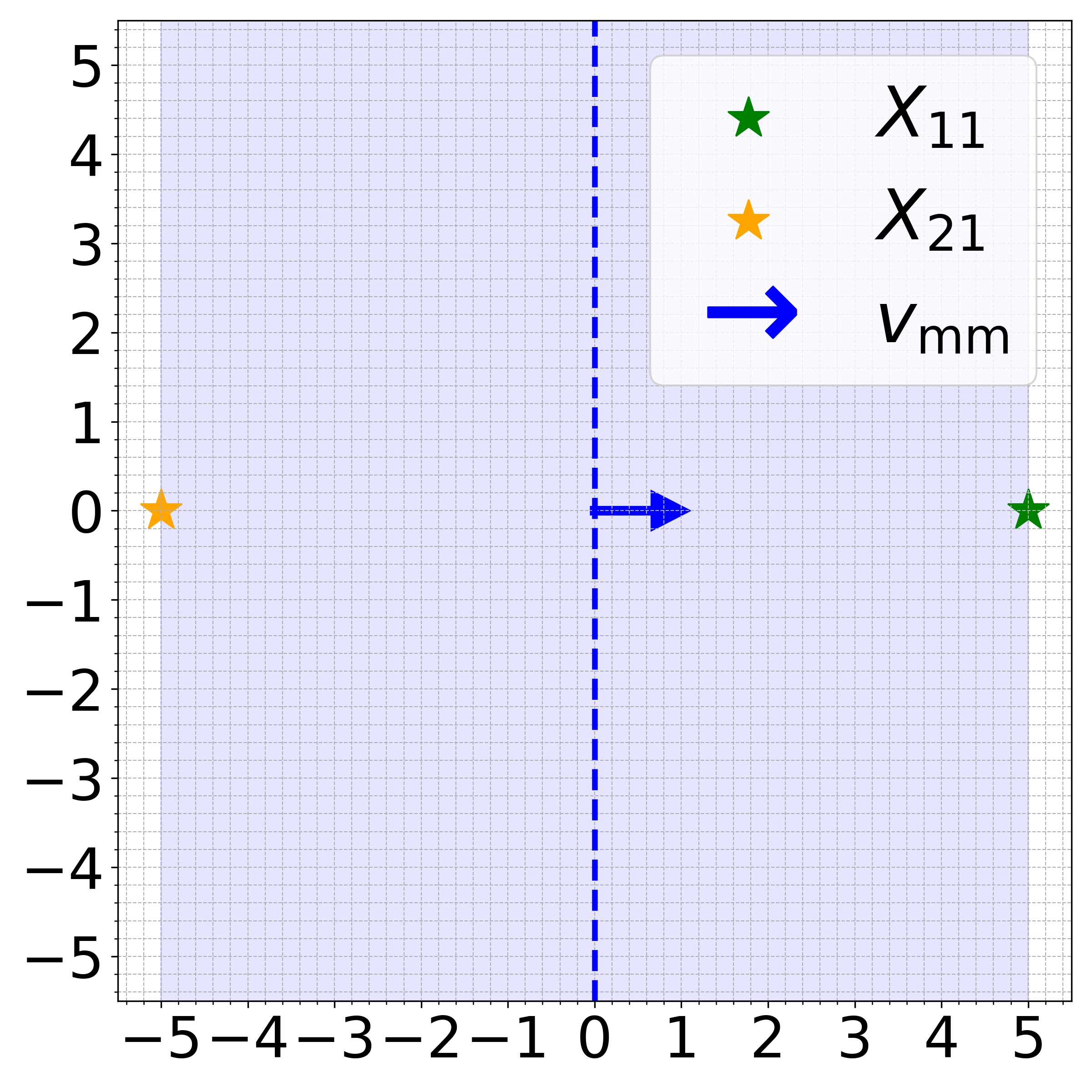
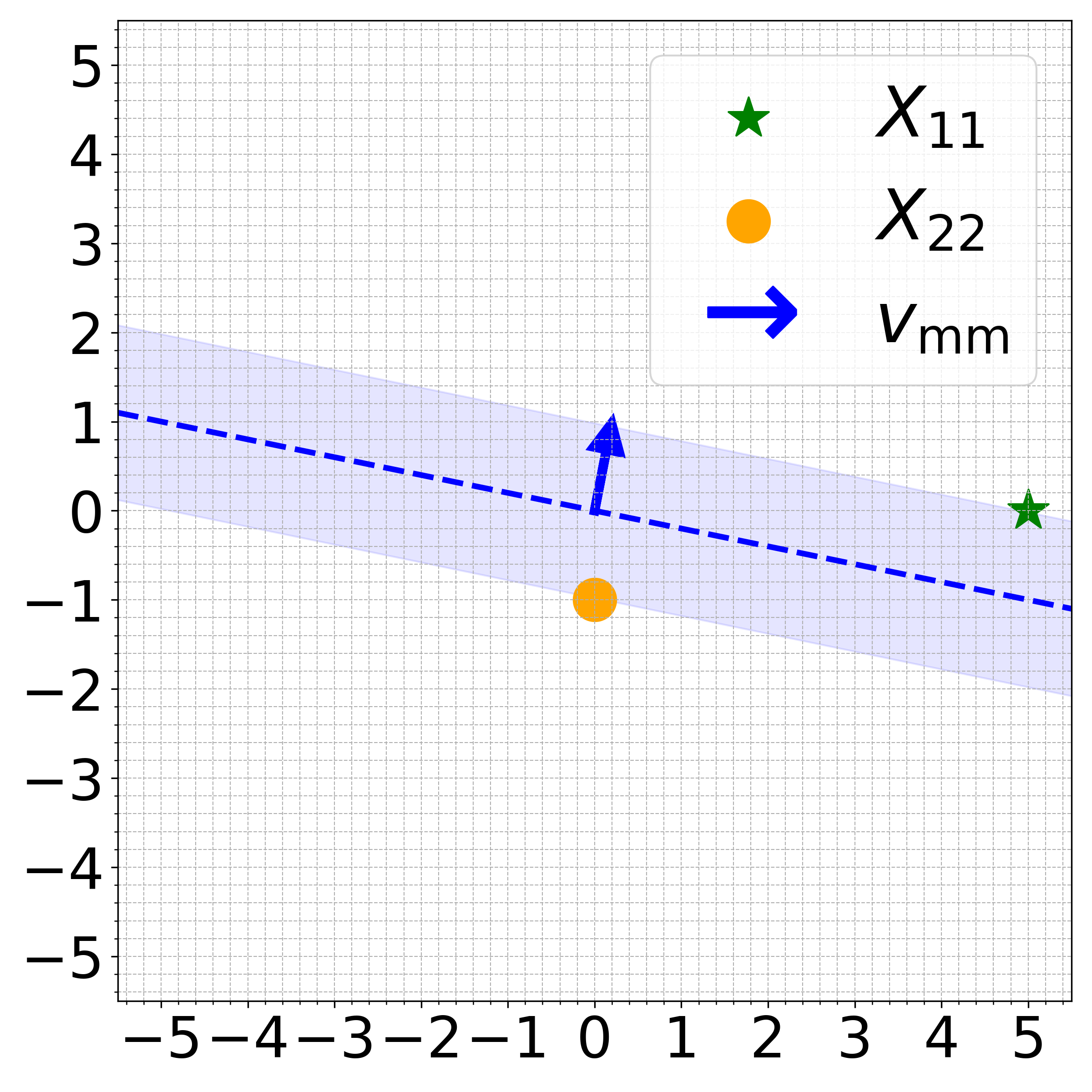
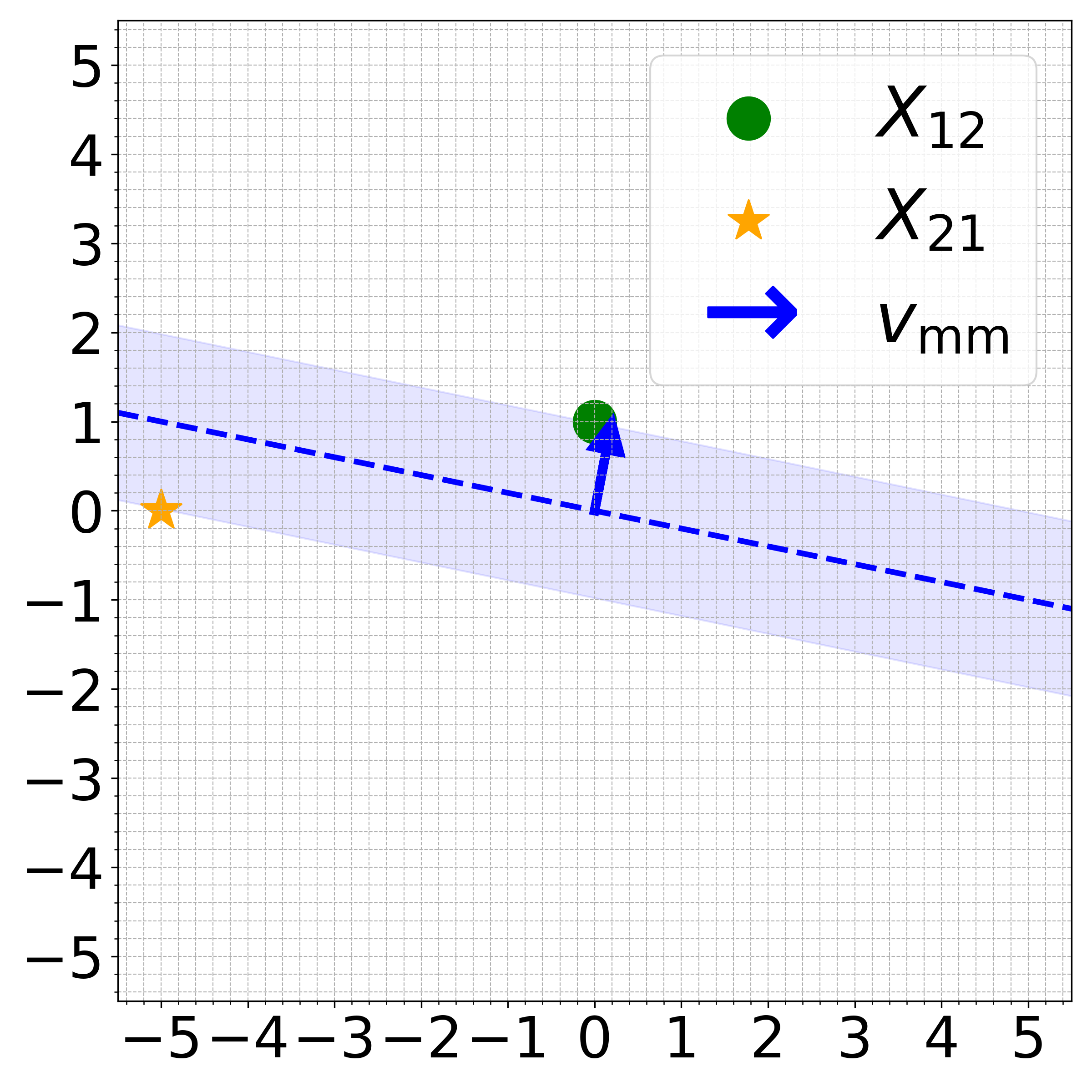
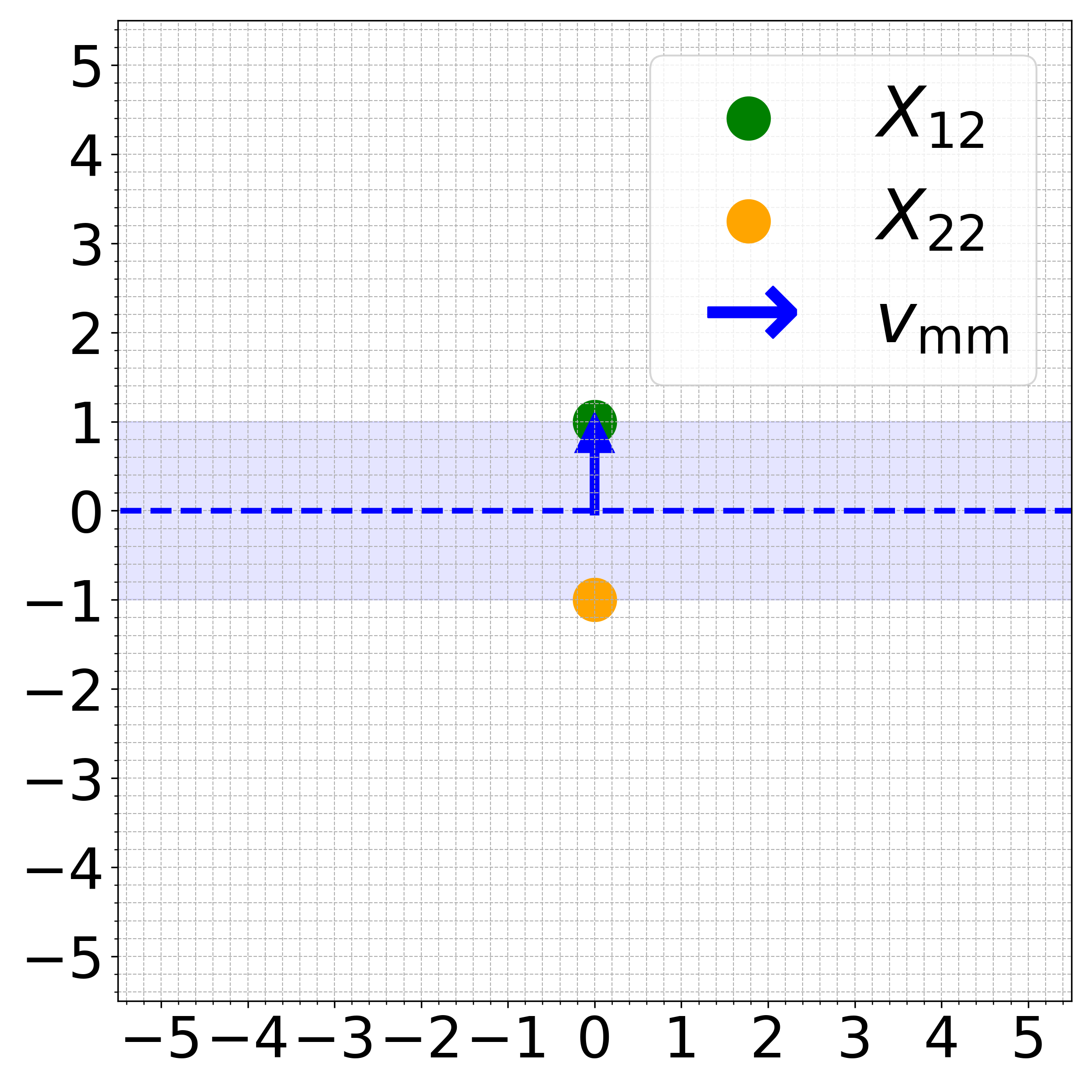
Consider the matrices X1=[5, 0; 0, 1]X_{1}=[5,\penalty\ 0;\penalty\ 0,\penalty\ 1] and X2=[5, 0; 0,1]X_{2}=[-5,\penalty\ 0;\penalty\ 0,\penalty\ -1] with y1=y2=1y_{1}=-y_{2}=1. Let Xi1X_{i1} be the optimal token and XitX_{it} be the others. Solving Problem ( ℓ p -AttSVM) with p=3p=3 and setting zi=Xi1z_{i}=X_{i1}, we obtain the solution Wmm:=Wmmα=[0.03846, 0;0.00769, 0]W_{\mathrm{mm}}:=W^{\alpha}_{\mathrm{mm}}=[0.03846,\penalty\ 0;\penalty\ -0.00769,\penalty\ 0]. Figure 1 illustrates how the optimal tokens X11X_{11} and X21X_{21} are separated by the dashed decision boundaries. These boundaries are orthogonal to the vectors WmmziW_{\mathrm{mm}}z_{i} and indicate the hyperplanes that separate the sequences based on the optimal token in each case.

Theorem 7 (p\ell_{p}–norm Regularization Path).

Suppose Assumption A on the loss function holds. Consider the ridge-constrained solutions W(R)W^{(R)} of (ERM) defined as

W(R):=argminWd×d(W)subj. toWp,pR.W^{(R)}:=\argmin_{W\in\mathbb{R}^{d\times d}}\penalty\ \mathcal{L}(W)\quad\textnormal{subj. to}\quad\|W\|_{p,p}\leq R. (p\ell_{p}-AttRP)

Then, limRW(R)/R=Wmmopt/Wmmoptp,p\lim_{R\to\infty}W^{(R)}/R=W^{\operatorname{opt}}_{\mathrm{mm}}/{\|W^{\operatorname{opt}}_{\mathrm{mm}}\|_{p,p}}, where WmmoptW^{\operatorname{opt}}_{\mathrm{mm}} is the solution of ( ℓ p -AttSVM), with αi\alpha_{i} replaced by opti\operatorname{opt}_{i}.

Theorem 7 shows that as the radius RR increases, the optimal direction W(R)W^{(R)} aligns more closely with the max-margin solution WmmαW^{\alpha}_{\mathrm{mm}}. This theorem, which allows for globally optimal tokens (see Definition 3), does not require any specific initialization for the ℓ p -AttRP algorithm and demonstrates that max-margin token separation is an essential feature of the attention mechanism.

Next, we analyze the convergence of MD applied to (ERM). Under specific initializations, the parameter’s p\ell_{p}-norm diverges to infinity, while its direction approaches the ( ℓ p -AttSVM) solution. To characterize these initializations, we define the following sets.

Definition 8.

Given a square matrix Wd×dW\in\mathbb{R}^{d\times d}, μ(0,1)\mu\in(0,1), and some R>0R>0,

Sp,μ(W)\displaystyle S_{p,\mu}(W) :={Wd×dDψ(WWp,p,WWp,p)μ},\displaystyle:=\left\{W^{\prime}\in\mathbb{R}^{d\times d}\mid D_{\psi}\left(\frac{W}{\|W\|_{p,p}},\frac{W^{\prime}}{\|W^{\prime}\|_{p,p}}\right)\leq\mu\right\}, (4a)
Cp,μ,R(W)\displaystyle C_{p,\mu,R}(W) :=Sμ(W){WWp,pR}.\displaystyle:=S_{\mu}(W)\cap\left\{W^{\prime}\mid\|W^{\prime}\|_{p,p}\geq R\right\}. (4b)

These sets contain matrices with a similar direction to a reference matrix WW, as captured by the inner product in Sμ(W)S_{\mu}(W). For Cp,μ,R(W)C_{p,\mu,R}(W), there is an additional constraint that the matrices must have a sufficiently high norm. We note that Sp,μ(W)S_{p,\mu}(W) and Cp,μ,R(W)C_{p,\mu,R}(W) reduce to their Euclidean variants as described in 60; 59 when p=2p=2. With this definition, we present our first theorem about the norm of the parameter increasing during training.

Theorem 9.

Suppose Assumption A holds. Let (αi)i=1n(\alpha_{i})_{i=1}^{n} be locally optimal tokens as per Definition 3. Consider the sequence W(k)W(k) generated by Algorithm ℓ p -AttGD. For a small enough stepsize η\eta, if W(0)Cp,μ,R(Wmmα)W(0)\in C_{p,\mu,R}(W^{\alpha}_{\mathrm{mm}}) for some dataset-dependent constants μ,R>0\mu,R>0, then we have W(k)p,p=Ω(logk)\|W(k)\|_{p,p}=\Omega(\log k).

Remark 10.

The condition on the stepsize η\eta is that it must be sufficiently small so that ψ()η()\psi(\cdot)-\eta\mathcal{L}(\cdot) remains convex for the matrices WW along the path traced by the iterates W(k)W(k). This applies to all theorems in this paper that require a sufficiently small stepsize η\eta.

This theorem implies that the parameters will increase and diverge to infinity, justifying the need to characterize the convergence of their direction.

Theorem 11 (Convergence of ℓ p -AttGD).

Suppose Assumption A holds. Let (αi)i=1n(\alpha_{i})_{i=1}^{n} be locally optimal tokens as per Definition 3. Consider the sequence W(k)W(k) generated by Algorithm ℓ p -AttGD. For a small enough stepsize η\eta, if W(0)Cp,μ,R(Wmmα)W(0)\in C_{p,\mu,R}(W^{\alpha}_{\mathrm{mm}}) for some dataset-dependent constants μ>0,R>exp(2)\mu>0,R>\textnormal{exp}(2), then

limkW(k)W(k)p,p=WmmαWmmαp,p.\lim_{k\rightarrow\infty}\frac{W(k)}{\|W(k)\|_{p,p}}=\frac{W^{\alpha}_{\mathrm{mm}}}{\|W^{\alpha}_{\mathrm{mm}}\|_{p,p}}.

These theorems show that as the parameters grow large enough and approach a locally optimal direction, they will keep moving toward that direction. While our results build on the max-margin token selection framework of 59, the extension to p\ell_{p}-mirror descent is nontrivial: we establish directional convergence under non-quadratic potentials where standard Euclidean arguments fail, and provide the first explicit finite-time poly-logarithmic convergence rates for attention optimization in Theorem 12.

Theorem 12 (Convergence Rate of ℓ p -AttGD).

Suppose Assumption A holds. Let (αi)i=1n(\alpha_{i})_{i=1}^{n} be locally optimal tokens as per Definition 3. Consider the sequence W(k)W(k) generated by Algorithm ℓ p -AttGD. For a small enough stepsize η\eta, if W(0)Cp,μ,R(Wmmα)W(0)\in C_{p,\mu,R}(W^{\alpha}_{\mathrm{mm}}) for some μ>0,R>exp(2)\mu>0,R>\textnormal{exp}(2), then

Dψ(WmmαWmmαp,p,W(k)W(k)p,p)=𝒪({loglogklogkifp>2,(loglogk)2logkifp=2,1(logk)p1otherwise.).D_{\psi}\left(\frac{W^{\alpha}_{\mathrm{mm}}}{\|W^{\alpha}_{\mathrm{mm}}\|_{p,p}},\frac{W(k)}{\|W(k)\|_{p,p}}\right)=\mathcal{O}\left(\begin{cases}\frac{\log\log k}{\log k}&\textnormal{if}\penalty\ \penalty\ p>2,\\ \frac{(\log\log k)^{2}}{\log k}&\textnormal{if}\penalty\ \penalty\ p=2,\\ \frac{1}{(\log k)^{p-1}}&\textnormal{otherwise}.\end{cases}\right). (5)

Establishing these rates required developing new analytical tools beyond the 2\ell_{2} blueprint: we prove p,p\ell_{p,p}-norm growth bounds under non-quadratic potentials (Lemma 4), introduce double-cone stability arguments to handle joint norm and directional constraints (Lemma 29), and work throughout with Bregman divergences rather than Euclidean geometry.

Figure 2: Illustration of Lemma 29. W(k)W(k), k>0\forall k>0 are within the larger set.

Note that in the left-hand side of (5), there is a dependence on pp in the Bregman divergence DψD_{\psi} itself as well. Despite optimizing a highly nonlinear, nonconvex softmax function, we achieve a convergence rate similar to GD in linear binary classification (34, Theorem 1.1) (up to a loglogk\log\log k factor).

Since we aim to show the parameter converges in direction to the cone center WmmαW_{\mathrm{mm}}^{\alpha}, we need conditions ensuring the parameters remain in the cone. Unlike 2\ell_{2} gradient descent where cone invariance follows from Pythagorean identities, the p\ell_{p} setting requires a novel double-cone construction: we must ensure iterates simultaneously remain within the directional cone Sp,μ0(Wmmα)S_{p,\mu_{0}}(W_{\mathrm{mm}}^{\alpha}) and satisfy the norm constraint Wp,pRπ\|W\|_{p,p}\geq R_{\pi}—a strictly joint requirement not present in prior mirror descent analyses (56). We formalize this in Lemma 29 and prove that for any μ>0\mu>0 and locally optimal tokens (αi)i=1n(\alpha_{i})_{i=1}^{n} (Definition 3), there exist constants R,μ>0R,\mu^{\prime}>0 depending on the dataset and μ\mu such that if W(0)Cp,μ,R(Wmmα)W(0)\in C_{p,\mu^{\prime},R}(W^{\alpha}_{\mathrm{mm}}), then W(k)Cp,μ,R(Wmmα)W(k)\in C_{p,\mu,R}(W^{\alpha}_{\mathrm{mm}}) for all kk, meaning the iterates remain within a larger cone; see Figure 2.

For Theorem 9, we show in Lemma 23 that at any timestep k0k\geq 0, the norm of the WW parameter evolves in the following manner,

|W(k+1)p,pp1\displaystyle|W(k+1)\|_{p,p}^{p-1} W(k)p,pp1+ηW(k)p,p(W(k)),W(k).\displaystyle\geq\|W(k)\|_{p,p}^{p-1}+\frac{\eta}{\|W(k)\|_{p,p}}\langle-\nabla\mathcal{L}(W(k)),W(k)\rangle.

With the above, to prove Theorem 9, it is enough to show that (W(k)),W(k)\langle-\nabla\mathcal{L}(W(k)),W(k)\rangle is positive and large enough to keep the norm increasing to infinity. Specifically, in Lemma 21 we show that there exist dataset-dependent constants R,δ,μ>0R,\delta,\mu>0 such that for all W,VCp,μ,R(Wmmα)W,V\in C_{p,\mu,R}(W^{\alpha}_{\mathrm{mm}}) with Vp,p=Wmmαp,p\|V\|_{p,p}=\|W^{\alpha}_{\mathrm{mm}}\|_{p,p},

(W),V=Ω(exp(Wp,pWmmαp,p(1+12δ)))>0.-\langle\nabla\mathcal{L}(W),V\rangle=\Omega\left(\textnormal{exp}\left(-\frac{\|W\|_{p,p}}{\|W^{\alpha}_{\mathrm{mm}}\|_{p,p}}\left(1+\frac{1}{2}\delta\right)\right)\right)>0.

Theorem 11 is a direct consequence of Theorem 12, which extends the analysis that is done for Lemma 29 by providing a tighter bound on how thin the cone set Cp,μ,RC_{p,\mu,R} may be for later iterates.

3.2 Training Dynamics of Mirror Descent for Joint Optimization of WW and vv

This section explores the training dynamics of jointly optimizing the prediction head vv and attention weights WW. Unlike Section 3.1, the main challenge here is the evolving token scores γ\gamma, as given in Definition 2, are influenced by the changing nature of vv. This requires additional technical considerations beyond those in Section 3.1, which are also addressed in this section.

Given stepsizes ηW,ηv>0\eta_{W},\eta_{v}>0, we consider the following joint updates for WW and vv applied to (ERM), respectively: for all i,j[d]i,j\in[d], and k=0,1,2,k=0,1,2,\dots,

{[W(k+1)]ij|[W(k)]ij+|1p1sign([W(k)]ij+),[W(k)]ij+:=|[W(k)]ij|p1sign([W(k)]ij)ηW[W(W(k),v(k))]ij,[v(k+1)]i|[v(k)]i+|1p1sign([v(k)]i+),[v(k)]i+:=|[v(k)]i|p1sign([v(k)]i)ηv[v(W(k),v(k))]i.\displaystyle\hskip-20.0pt\begin{cases}\left[W(k+1)\right]_{ij}\leftarrow\left|[W(k)]^{+}_{ij}\right|^{\frac{1}{p-1}}\cdot\textnormal{sign}\left([W(k)]^{+}_{ij}\right),\vskip 8.5359pt\\ [W(k)]^{+}_{ij}:=|[W(k)]_{ij}|^{p-1}\textnormal{sign}([W(k)]_{ij})-\eta_{W}[\nabla_{W}\mathcal{L}(W(k),v(k))]_{ij},\vskip 8.5359pt\\ [v(k+1)]_{i}\leftarrow\left|[v(k)]_{i}^{+}\right|^{\frac{1}{p-1}}\cdot\textnormal{sign}([v(k)]_{i}^{+}),\vskip 8.5359pt\\ [v(k)]_{i}^{+}:=|[v(k)]_{i}|^{p-1}\textnormal{sign}([v(k)]_{i})-\eta_{v}[\nabla_{v}\mathcal{L}(W(k),v(k))]_{i}.\end{cases} (p\ell_{p}-JointGD)

We discuss the implicit bias and convergence for v(k)v(k) below. From previous results (3), one can expect v(k)v(k) to converge to the p\ell_{p}-SVM solution, i.e., the max-margin classifier separating the set of samples {(Xiαi,yi)}i=1n\{(X_{i\alpha_{i}},y_{i})\}_{i=1}^{n}, where XiαiX_{i\alpha_{i}} denote the (locally) optimal token for each i[n]i\in[n]. Consequently, we consider the following hard-margin SVM problem,

vmm:=argminvdvpsubj. toyiXiαiv1,for all i[n].\begin{split}v_{\mathrm{mm}}&:=\argmin_{v\in\mathbb{R}^{d}}\|v\|_{p}\\ &\textnormal{subj.\penalty\ to}\penalty\ \penalty\ \penalty\ y_{i}X_{i\alpha_{i}}^{\top}v\geq 1,\penalty\ \penalty\ \textnormal{for all }\penalty\ i\in[n].\end{split} (p\ell_{p}-SVM)
Refer to caption
Refer to caption
Refer to caption
Refer to caption
Figure 3: Effect of token selection on margin size in ( ℓ p -SVM) for Example 6. The first plot shows the largest class margin with optimal tokens X11X_{11} and X21X_{21}. In subsequent plots, as different tokens are used, the class margin (light blue shaded area) decreases, reflecting suboptimal class separation.

In ( ℓ p -SVM), define the label margin as 1/vmmp1/\|v_{\mathrm{mm}}\|_{p}. The label margin quantifies the distance between the separating hyperplane and the nearest data point in the feature space. A larger label margin indicates better generalization performance of the classifier, as it suggests that the classifier has a greater separation between classes. From ( ℓ p -SVM) and Definitions 2 and 3, an additional intuition by 60 behind optimal tokens is that they maximize the label margin when selected; see Figure 3. Selecting the locally optimal token indices α=(αi)i=1n\alpha=(\alpha_{i})_{i=1}^{n} from each input data sequence achieves the largest label margin, meaning that including other tokens will reduce the label margin as defined in ( ℓ p -SVM). In the Appendix F, we show that WW and vv generated by ℓ p -JointRP converge to their respective max-margin solutions under suitable geometric conditions (Theorem 32 in the appendix).

4 Experimental Results

4.1 Synthetic Data Experiments

We describe the setup of the experiments for ℓ p -AttGD and ℓ p -JointGD and their results.

4.1.1 ℓ p -AttGD Experiment

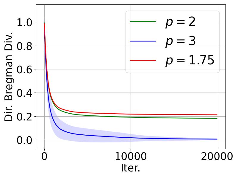
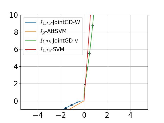
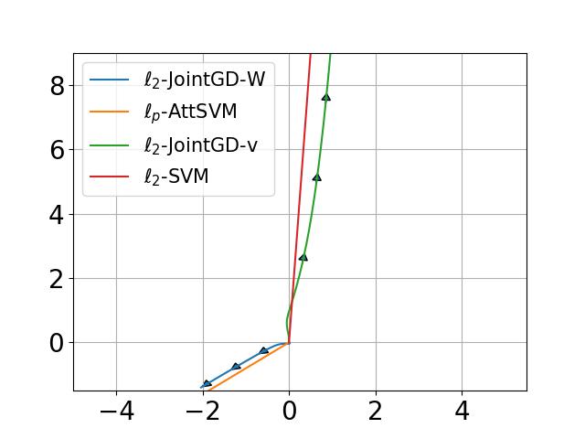
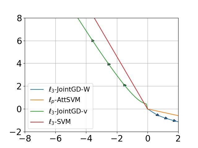
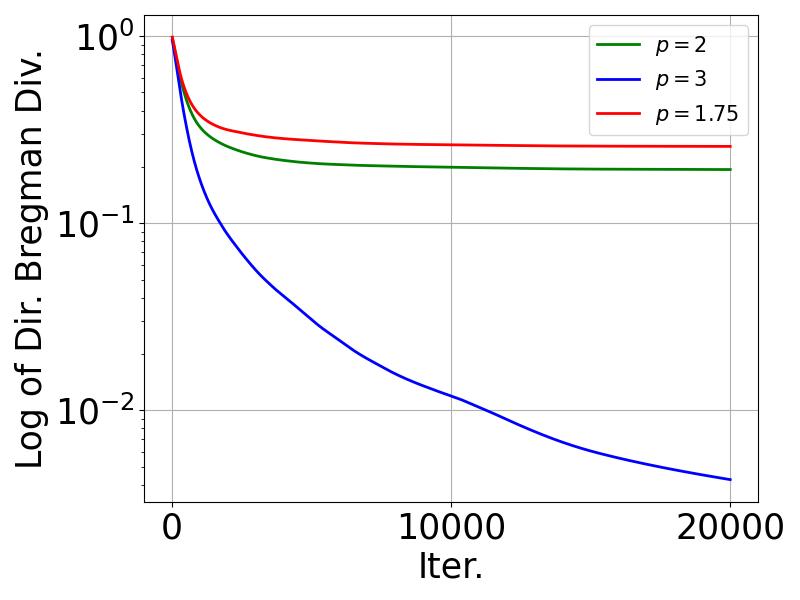
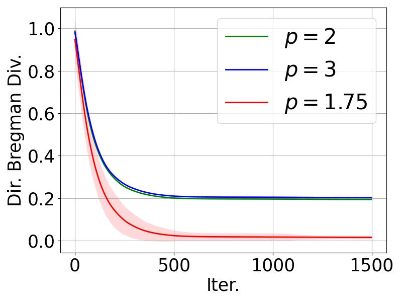
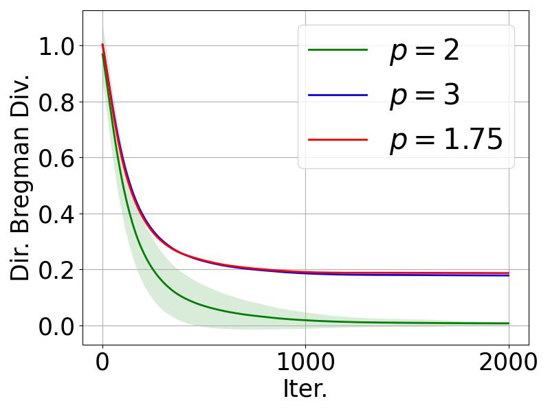
To measure the directional distance between WαmmW^{\mathrm{mm}}_{\alpha} (solution of ( ℓ p -AttSVM)) and W(k)W(k) (output of ℓ p -AttGD), we use the directional Bregman divergence Dψ(W/Wp,p,V/Vp,p)D_{\psi}(W/\|W\|_{p,p},V/\|V\|_{p,p}) for W,Vd×dW,V\in\mathbb{R}^{d\times d}. We compare the ( ℓ p -AttSVM) solution with the q\ell_{q} optimization path for all p,q{1.75,2,3}p,q\in\{1.75,2,3\} for synthetically generated data (described in detail in the Appendix). The experiment is repeated 100 times, and the average directional Bregman divergence is reported. A closer look at one sample trial is also provided.
Refer to caption
(a) 1.75\ell_{1.75} Dir. Bregman Div.
Refer to caption
(b) 2\ell_{2} Directional Bregman Div.
Refer to caption
(c) 3\ell_{3} Directional Bregman Div.
Figure 4: Average directional Bregman divergence between the (a) 1.75\ell_{1.75}, (b) 2\ell_{2}, and (c) 3\ell_{3} optimization paths and the ( ℓ p -AttSVM) solutions for p=1.75,2p=1.75,2, and 33 at each training iteration from 100 trials. The shaded area represents the standard deviation of the directional Bregman divergence.
Refer to caption
(a) 1.75\ell_{1.75} Optimization Path
Refer to caption
(b) 2\ell_{2} Optimization Path
Refer to caption
(c) 3\ell_{3} Optimization Path
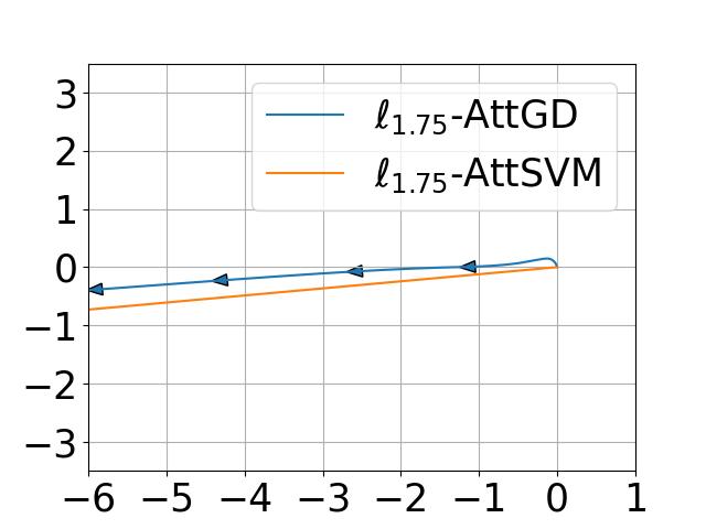
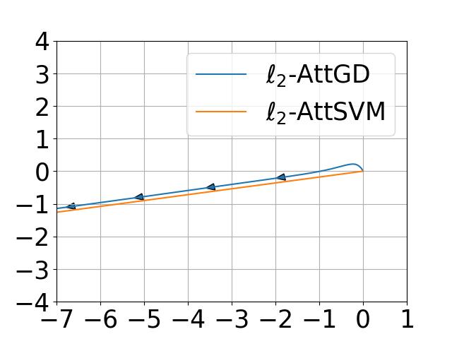
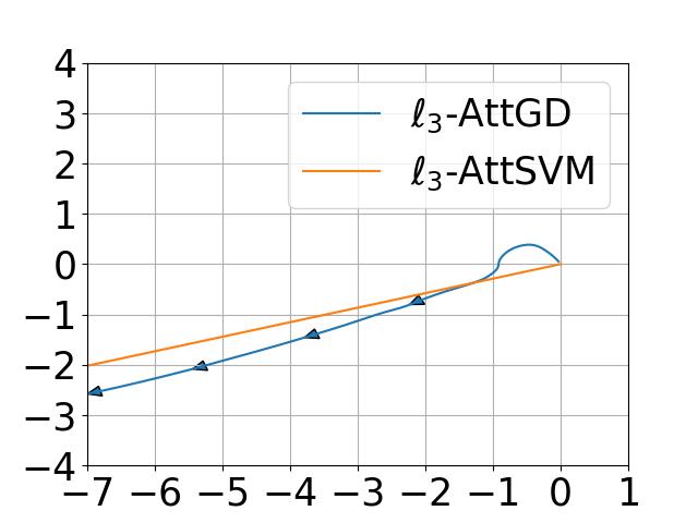
Figure 5: Direction of change of two entries of WW updated by ℓ p -AttGD with p=1.75p=1.75, p=2p=2, and p=3p=3 for one trial, shown in (a), (b), and (c). Each axis represents a different entry. The orange line shows the direction of ( ℓ p -AttSVM).

Figure 4 shows the directional Bregman divergence between the ( ℓ p -AttSVM) solution and the q\ell_{q} optimization path for each pair p,q{1.75,2,3}p,q\in\{1.75,2,3\}. In Figure 4(a), the divergence converges to 00 only for the ( ℓ p -AttSVM) (p=1.75p=1.75) solution, indicating that the 1.75\ell_{1.75} path does not converge to the p=2p=2 or 33 solutions. The shrinking standard deviation shows consistent behavior. Similarly, Figures 4(b) and 4(c) show the divergence converging to 00 for the corresponding ( ℓ p -AttSVM) solution, demonstrating that the p\ell_{p} optimization path converges to the ( ℓ p -AttSVM) solution, with the direction of convergence changing with pp. In addition to the directional Bregman divergence, we can also observe the convergence in direction for one trial (initialized at zero) directly by plotting how two of the entries of WW change during training simultaneously and plotting it on a Cartesian graph, then showing that the path it follows converges to the direction of the ( ℓ p -AttSVM) solution. As we can see in Figure 5, each of the p\ell_{p} optimization paths follows the direction of the corresponding ( ℓ p -AttSVM) solution.

4.1.2 ℓ p -JointGD Experiments

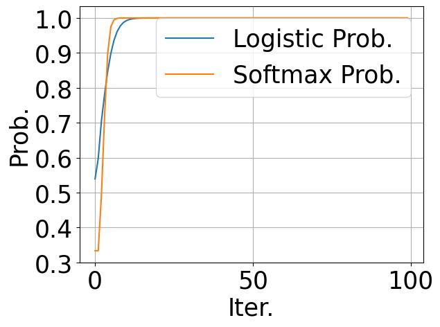
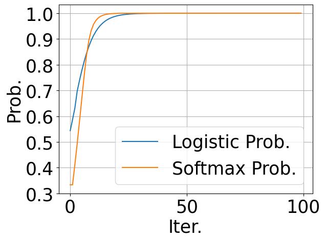
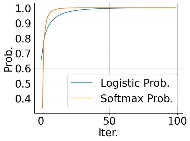
We use the data from Example 34 in Appendix G.3 to train a model using ℓ p -JointGD for p=1.75,2,p=1.75,2, and 33. The comparison between the iterates and the SVM solutions in Figure 6 shows that the iterates of WW and vv converge to the ℓ p -AttSVM and ℓ p -SVM directions, respectively, for each of p=1.75,2,p=1.75,2, and 33. These convergence are similar to Theorem 32, as in both this experiment and that theorem, we get that the iterates converge to the SVM problem solutions. In addition to these iterates, we record the evolution of the average softmax probability of the optimal token, along with the average logistic probability of the model, which we define to be 1/ni=1n1/(1+exp(γiai))1/n\sum_{i=1}^{n}1/(1+\exp(-\gamma_{i}a_{i})).

Refer to caption
(a) 1.75\ell_{1.75} Optimization Paths
Refer to caption
(b) 2\ell_{2} Optimization Paths
Refer to caption
(c) 3\ell_{3} Optimization Paths
Figure 6: Iterates of the WW and vv parameters of the model as they are trained using ℓ p -JointGD for p=1.75,2,p=1.75,2, and 33, along with the corresponding ℓ p -AttSVM and ℓ p -SVM directions.
Refer to caption
(a) 1.75\ell_{1.75} Probabilties
Refer to caption
(b) 2\ell_{2} Probabilties
Refer to caption
(c) 3\ell_{3} Probabilties
Figure 7: Softmax probability evolution of the optimal token and logistic probability evolution for p=1.75,2,p=1.75,2, and 33.

As shown in Figure 7, each average softmax probability converges to 11, indicating that the attention mechanism produces a softmax vector converging to a one-hot vector during different ℓ p -JointGD training. Moreover, the average logistic probability also converges to 11, indicating the model’s prediction reaches 100%100\% accuracy.

4.2 Real Data Experiments

This section presents evidence of improved generalization, token selection, and explainability from training an attention network with MD instead of other algorithms such as GD and Adam (38). Specifically, we compare the generalization, token selection, and model weight distribution of the MD and GD algorithms in training a transformer classification model on the Stanford Large Movie Review Dataset; and the generalization and model weight distribution of the MD and Adam in training a vision transformer (ViT) model (21) on CIFAR-10.

4.2.1 Comparison with Gradient Descent

Algorithm Model Size 3 Model Size 4 Model Size 6
1.1\ell_{1.1}-MD 83.47 ±\pm 0.09% 83.36 ±\pm 0.13% 83.65 ±\pm 0.13%
2\ell_{2}-MD 81.66±0.09%81.66\pm 0.09\% 81.05±0.17%81.05\pm 0.17\% 82.22±0.13%82.22\pm 0.13\%
3\ell_{3}-MD 82.57±0.09%82.57\pm 0.09\% 82.40±0.12%82.40\pm 0.12\% 81.97±0.10%81.97\pm 0.10\%
Table 1: Test accuracies of transformer classification models trained with 1.1\ell_{1.1}, 2\ell_{2}, and 3\ell_{3}-MD on the Stanford Large Movie Review Dataset. The model sizes refers to the number of layers in the transformer model and the number of attention heads per layer. 1.1\ell_{1.1}-MD provides superior generalization performance.

We trained a transformer classification model on the Stanford Large Movie Review Dataset (43) using MD with 1.1\ell_{1.1}, 2\ell_{2}, and 3\ell_{3} potentials. The models are similar to the encoder module in 68, with the last layer being a linear classification layer on the feature representation of the first [CLS][\texttt{CLS}] token. We put the details of the classification model in Appendix G.4. Table 1 summarizes the resulting test accuracy of several variants of that model when trained with the three algorithms, which shows that the 1.1\ell_{1.1} potential MD outperforms the other MD algorithms, including the one with the 2\ell_{2} potential, which is equivalent to the GD.
Refer to caption
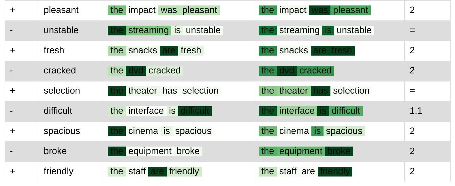
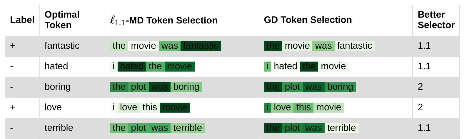
Figure 8: The attention map generated by the resulting models that were trained using 1.1\ell_{1.1}MD and GD for five sample sentences. For three out of five of the sample sentences, the model trained using 1.1\ell_{1.1}MD selects the optimal token better than the model trained using GD.

To investigate this further, we look at how the attention layers of the model select the tokens from simple reviews that GPT-4o generated and investigate how much the attention layer focuses on a particular token that truly determines whether the whole review was a positive one or a negative one. We chose these pivotal tokens using GPT-4o as well. We do this procedure to the model trained using 1.1\ell_{1.1}MD and the GD and tabulate the full results in Appendix G (we provide five of the results in Figure 8). We can see that the 1.1\ell_{1.1}MD also outperforms the GD in token selection.
Refer to caption
(a)
Refer to caption
(b)
Refer to caption
(c)
Refer to caption
(d)
Refer to caption
(e)
Refer to caption
(f)
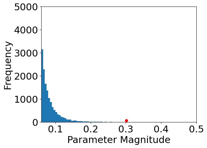
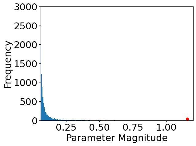
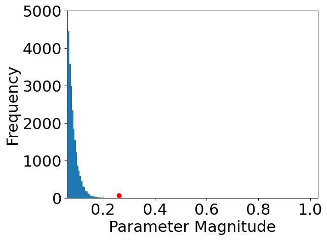
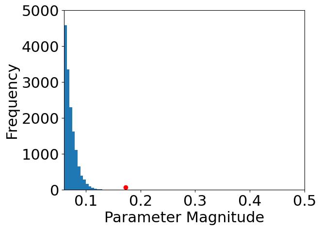
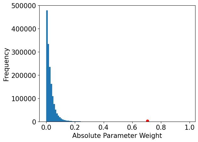
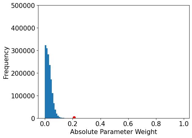
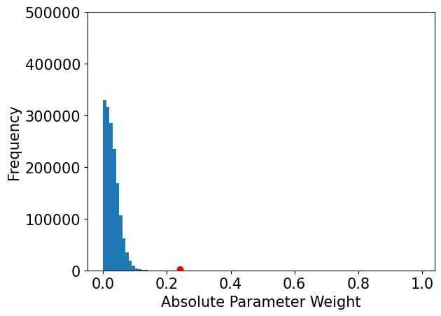
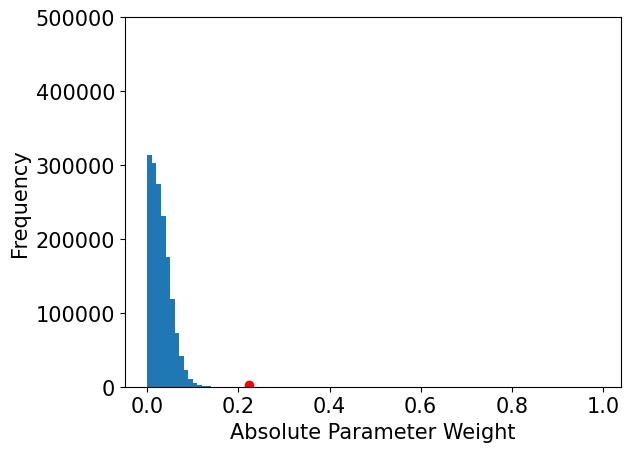
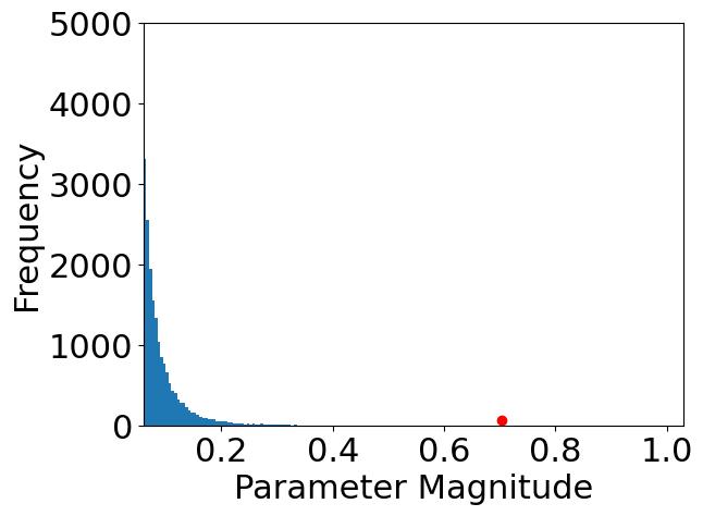
Figure 9: Histogram of the absolute values of the WK,WQ,W_{K},W_{Q}, and WVW_{V} components of transformer models trained with 1.1\ell_{1.1} and 2\ell_{2}-MD on the Stanford Large Movie Review Dataset. Only large parameters (0.06\geq 0.06) are shown, with the maximum magnitude component marked by a red dot. The 1.1\ell_{1.1}-MD model has 18,20618,206 components in WKW_{K}, 13,96413,964 in WQW_{Q}, and 7,6437,643 in WVW_{V} with magnitudes 0.06\geq 0.06, while the 2\ell_{2}-MD model has 27,22427,224 in WKW_{K}, 14,65414,654 in WQW_{Q}, and 10,12710,127 in WVW_{V} with such magnitudes. These results imply that the 1.1\ell_{1.1}-MD algorithm yields sparser parameters and that it would have a stronger token selection ability.

Finally, we collect the training weights from the resulting models trained by 1.1\ell_{1.1}MD and the GD and plot a histogram of their absolute values in Figure 9. Specifically, we take the histogram of the components of the key, query, and value matrices. The figures show that the resulting model that was trained using 1.1\ell_{1.1}MD is sparser than the one trained using GD, which could hint at a potential explanation as to why 1.1\ell_{1.1}MD can outperform the standard GD algorithm when it is used to train attention-based models.

4.2.2 Comparison with Adam

We compare the 1.1,1.75,2,3\ell_{1.1},\ell_{1.75},\ell_{2},\ell_{3}MD, and Adam algorithms in training a ViT model on the CIFAR-10 dataset. We specify the ViT model architecture in Appendix G.5.

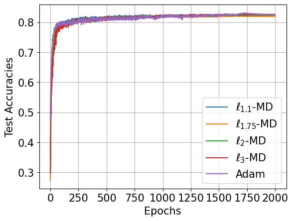
The resulting test accuracies for all algorithms are reported in Figure . Notably, all five optimization methods—spanning the p\ell_{p}-MD family with p{1.1,1.75,2,3}p\in\{1.1,1.75,2,3\} and Adam—converge to approximately 82%82\% test accuracy on CIFAR-10, demonstrating that our p\ell_{p}-MD framework achieves state-of-the-art performance competitive with widely-used adaptive optimizers. The consistent performance across different values of pp confirms that the beneficial sparsity and interpretability properties induced by the p\ell_{p} geometry (particularly for pp close to 1) come at no cost to generalization capability.
Refer to caption
(a)
Refer to caption
(b)
Figure 10: Test accuracy comparison across different optimizers on CIFAR-10 and -100.

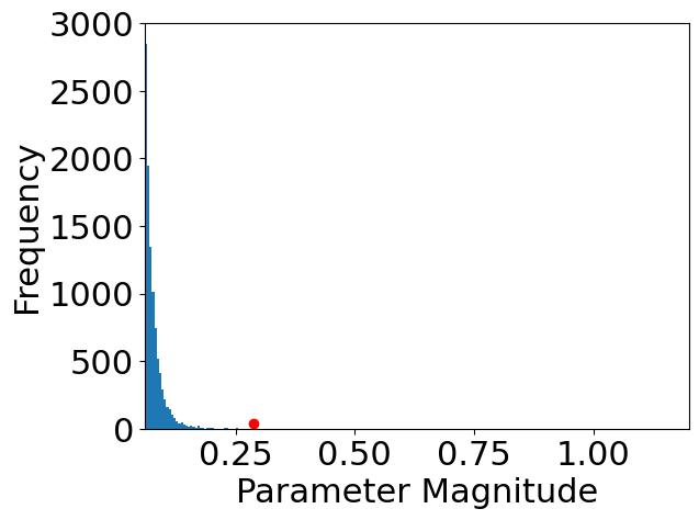
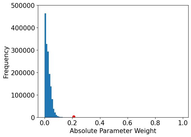
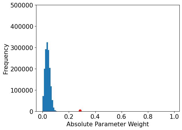
Furthermore, we examine the learned weight distributions by plotting the absolute values of attention layer parameters (key, query, and value matrices) from models trained with different optimizers in Figure 11. Consistent with our earlier observations in Figure 9, 1.1\ell_{1.1}-MD produces markedly sparser attention weights compared to Adam, with a substantially higher concentration of near-zero parameters. This sparsity pattern reveals that 1.1\ell_{1.1}-MD implicitly performs feature selection during training, concentrating representational capacity on the most discriminative attention components while driving less relevant weights toward zero. Such induced sparsity not only enhances model interpretability by identifying which attention mechanisms are critical for the task, but also enables more aggressive pruning and compression strategies without sacrificing performance—a practical advantage for deployment in resource-constrained environments.

Refer to caption
(a)
Refer to caption
(b)
Refer to caption
(c)
Refer to caption
(d)
Refer to caption
(e)
Refer to caption
(f)
Figure 11: Histogram of the absolute values of the WK,WQ,W_{K},W_{Q}, and WVW_{V} components of ViT models trained with 1.1\ell_{1.1}-MD and Adam on CIFAR-10. These results show that 1.1\ell_{1.1}-MD can be more explainable compared to Adam because it produces sparser parameters, which should induce better token selection.

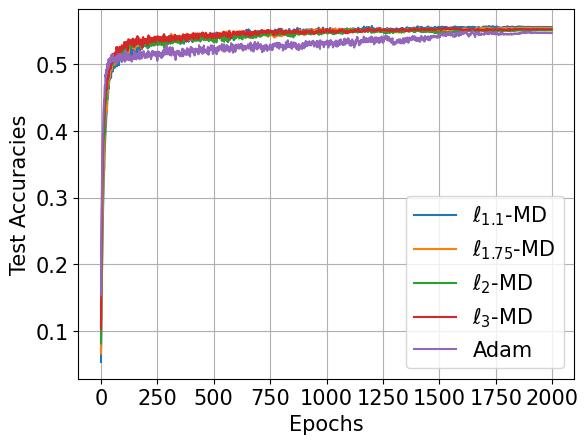
Similarly, we also compare these algorithms in training the same ViT architecture on CIFAR-100, a more complex dataset.

The results in Figure show that our MD algorithms generally achieve test scores of around 55%55\%, which are at a similar level to those of other popular training algorithms, such as SGD and Adam, on CIFAR-100, further demonstrating that our algorithms can compete with the state-of-the-art. Again, we plot histograms of the absolute values of the key, query, and value weights in the attention layers of the resulting models that were trained using Adam and 1.1\ell_{1.1}MD. Figure 12 shows these histograms, and as we can see, the resulting model trained by 1.1\ell_{1.1}MD has significantly more attention weight entries that are close to zero when compared to the model trained by Adam, making the attention weights sparser.

Refer to caption
(a)
Refer to caption
(b)
Refer to caption
(c)
Refer to caption
(d)
Refer to caption
(e)
Refer to caption
(f)
Figure 12: Histogram of the absolute values of the entries in the WK,WQW_{K},W_{Q}, and WVW_{V} attention weight matrices of the resulting models trained by 1.1\ell_{1.1}MD and Adam on CIFAR-100. We can see that the weights from the model that was trained by 1.1\ell_{1.1}MD is more sparse. The red dot represent the maximum absolute values of the respective weight matrices.

5 Conclusion and Future Work

We explored the optimization dynamics and generalization performance of a family of MD algorithms for softmax attention mechanisms, focusing on ℓ p -AttGD, which generalizes GD by using the pp-th power of the p\ell_{p}-norm as the potential function. Our theoretical analysis and experiments show that ℓ p -AttGD converges to the solution of a generalized hard-margin SVM with an p\ell_{p}-norm objective in classification tasks using a single-layer softmax attention model. This generalized SVM separates optimal from non-optimal tokens via linear constraints on token pairs. We also examined the joint problem under logistic loss with p\ell_{p}-norm regularization and proved that WW and vv generated by p\ell_{p}-norm regularization path converge to their respective generalized max-margin solutions. Finally, our numerical experiments on real data demonstrate that MD algorithms improve generalization over standard GD and excel in optimal token selection.

Our theoretical guarantees are established for single-head, one-layer attention models—a standard abstraction that balances analytical tractability with capturing the essential nonconvex structure of softmax attention. An important direction for future work is extending these convergence results to multi-head and multi-layer architectures, where each head solves separation problems in different subspaces and stacked layers progressively refine feature representations.

acknowledgments-disclosure-of-funding.
The authors acknowledge the MIT SuperCloud and Lincoln Laboratory Supercomputing Center for providing computing resources that have contributed to the results reported within this paper. This work was supported in part by MathWorks, Jane Street, the MIT-IBM Watson AI Lab, the MIT-Amazon Science Hub, and the MIT-Google Program for Computing Innovation. The authors also thank Roey Magen for valuable feedback on the joint regularization path analysis.

References

  • Arora et al. (2019) S. Arora, N. Cohen, W. Hu, and Y. Luo Implicit regularization in deep matrix factorization. Advances in Neural Information Processing Systems 32. Cited by: §1.2.
  • Azizan and Hassibi (2018) N. Azizan and B. Hassibi Stochastic gradient/mirror descent: minimax optimality and implicit regularization. In International Conference on Learning Representations, Cited by: §A.4, §1.1, §1.2.
  • Azizan et al. (2021) N. Azizan, S. Lale, and B. Hassibi Stochastic mirror descent on overparameterized nonlinear models. IEEE Transactions on Neural Networks and Learning Systems 33 (12), pp. 7717–7727. Cited by: §1.1, §3.1, §3.2.
  • Bahdanau et al. (2014) D. Bahdanau, K. Cho, and Y. Bengio Neural machine translation by jointly learning to align and translate. arXiv preprint arXiv:1409.0473. Cited by: §1.
  • Bao et al. (2024) H. Bao, R. Hataya, and R. Karakida Self-attention networks localize when qk-eigenspectrum concentrates. arXiv preprint arXiv:2402.02098. Cited by: §1.2.
  • Bauschke et al. (2017) H. H. Bauschke, J. Bolte, and M. Teboulle A descent lemma beyond lipschitz gradient continuity: first-order methods revisited and applications. Mathematics of Operations Research 42 (2), pp. 330–348. Cited by: §2.
  • Blair (1985) C. Blair Problem complexity and method efficiency in optimization (a. s. nemirovsky and d. b. yudin). SIAM Review 27 (2), pp. 264–265. External Links: Document Cited by: §2.
  • Bregman (1967) L. M. Bregman The relaxation method of finding the common point of convex sets and its application to the solution of problems in convex programming. USSR computational mathematics and mathematical physics 7 (3), pp. 200–217. Cited by: §A.4, §1.1, §2, Lemma 27.
  • Bubeck et al. (2015) S. Bubeck et al. Convex optimization: algorithms and complexity. Foundations and Trends® in Machine Learning 8 (3-4), pp. 231–357. Cited by: §2.
  • Chen et al. (2021a) L. Chen, K. Lu, A. Rajeswaran, K. Lee, A. Grover, M. Laskin, P. Abbeel, A. Srinivas, and I. Mordatch Decision transformer: reinforcement learning via sequence modeling. In Advances in Neural Information Processing Systems, Vol. 34, pp. 15084–15097. Cited by: §1.
  • Chen et al. (2021b) M. Chen, J. Tworek, H. Jun, Q. Yuan, H. P. d. O. Pinto, J. Kaplan, H. Edwards, Y. Burda, N. Joseph, G. Brockman, et al. Evaluating large language models trained on code. arXiv preprint arXiv:2107.03374. Cited by: §1.
  • Chen and Li (2024) S. Chen and Y. Li Provably learning a multi-head attention layer. arXiv preprint arXiv:2402.04084. Cited by: §1.2.
  • Chen and Li (2025) S. Chen and Y. Li Provably learning a multi-head attention layer. In Proceedings of the 57th Annual ACM Symposium on Theory of Computing, pp. 1744–1754. Cited by: §1.2.
  • Chen et al. (2024a) S. Chen, H. Sheen, T. Wang, and Z. Yang Training dynamics of multi-head softmax attention for in-context learning: emergence, convergence, and optimality. arXiv preprint arXiv:2402.19442. Cited by: §1.2.
  • Chen et al. (2024b) Y. Chen, Q. Tao, F. Tonin, and J. Suykens Primal-attention: self-attention through asymmetric kernel svd in primal representation. Advances in Neural Information Processing Systems 36. Cited by: §1.2.
  • Chizat and Bach (2020) L. Chizat and F. Bach Implicit bias of gradient descent for wide two-layer neural networks trained with the logistic loss. In Conference on learning theory, pp. 1305–1338. Cited by: §1.2.
  • Collins et al. (2024) L. Collins, A. Parulekar, A. Mokhtari, S. Sanghavi, and S. Shakkottai In-context learning with transformers: softmax attention adapts to function lipschitzness. arXiv preprint arXiv:2402.11639. Cited by: §1.2, §1.2.
  • Deng et al. (2023) Y. Deng, Z. Song, S. Xie, and C. Yang Unmasking transformers: a theoretical approach to data recovery via attention weights. arXiv preprint arXiv:2310.12462. Cited by: §1.2.
  • Deora et al. (2023) P. Deora, R. Ghaderi, H. Taheri, and C. Thrampoulidis On the optimization and generalization of multi-head attention. arXiv preprint arXiv:2310.12680. Cited by: §1.2, §1.2.
  • Devlin et al. (2019) J. Devlin, M. Chang, K. Lee, and K. Toutanova BERT: pre-training of deep bidirectional transformers for language understanding. In Proceedings of the 2019 Conference of the North American Chapter of the Association for Computational Linguistics: Human Language Technologies, Volume 1 (Long and Short Papers), Minneapolis, Minnesota, pp. 4171–4186. Cited by: §1.
  • Dosovitskiy et al. (2021a) A. Dosovitskiy, L. Beyer, A. Kolesnikov, D. Weissenborn, X. Zhai, T. Unterthiner, M. Dehghani, M. Minderer, G. Heigold, S. Gelly, et al. An image is worth 16x16 words: transformers for image recognition at scale. In International Conference on Learning Representations, Cited by: §G.5, §4.2.
  • Dosovitskiy et al. (2021b) A. Dosovitskiy, L. Beyer, A. Kolesnikov, D. Weissenborn, X. Zhai, T. Unterthiner, M. Dehghani, M. Minderer, G. Heigold, S. Gelly, J. Uszkoreit, and N. Houlsby An image is worth 16x16 words: transformers for image recognition at scale. In International Conference on Learning Representations, Cited by: §1.
  • Driess et al. (2023) D. Driess, F. Xia, M. S. Sajjadi, C. Lynch, A. Chowdhery, B. Ichter, A. Wahid, J. Tompson, Q. Vuong, T. Yu, et al. Palm-e: an embodied multimodal language model. arXiv preprint arXiv:2303.03378. Cited by: §1.
  • Ergen et al. (2022) T. Ergen, B. Neyshabur, and H. Mehta Convexifying transformers: improving optimization and understanding of transformer networks. arXiv:2211.11052. Cited by: §1.2.
  • Frei et al. (2022) S. Frei, G. Vardi, P. L. Bartlett, N. Srebro, and W. Hu Implicit bias in leaky relu networks trained on high-dimensional data. arXiv preprint arXiv:2210.07082. Cited by: §1.2.
  • Fu et al. (2023) D. Fu, T. Chen, R. Jia, and V. Sharan Transformers learn higher-order optimization methods for in-context learning: a study with linear models. arXiv preprint arXiv:2310.17086. Cited by: §1.2.
  • Gunasekar et al. (2018) S. Gunasekar, J. Lee, D. Soudry, and N. Srebro Characterizing implicit bias in terms of optimization geometry. In International Conference on Machine Learning, pp. 1832–1841. Cited by: §1.2.
  • Huang et al. (2024) R. Huang, Y. Liang, and J. Yang Non-asymptotic convergence of training transformers for next-token prediction. arXiv preprint arXiv:2409.17335. Cited by: §1.2.
  • Huang et al. (2023) Y. Huang, Y. Cheng, and Y. Liang In-context convergence of transformers. arXiv preprint arXiv:2310.05249. Cited by: §1.2.
  • Ildiz et al. (2024) M. E. Ildiz, Y. Huang, Y. Li, A. S. Rawat, and S. Oymak From self-attention to markov models: unveiling the dynamics of generative transformers. arXiv preprint arXiv:2402.13512. Cited by: §1.2.
  • Jelassi et al. (2022) S. Jelassi, M. E. Sander, and Y. Li Vision transformers provably learn spatial structure. In Advances in Neural Information Processing Systems, A. H. Oh, A. Agarwal, D. Belgrave, and K. Cho (Eds.), Cited by: §1.2.
  • Jeon et al. (2024) H. J. Jeon, J. D. Lee, Q. Lei, and B. Van Roy An information-theoretic analysis of in-context learning. arXiv preprint arXiv:2401.15530. Cited by: §1.2.
  • Ji et al. (2021) Z. Ji, N. Srebro, and M. Telgarsky Fast margin maximization via dual acceleration. In International Conference on Machine Learning, pp. 4860–4869. Cited by: §1.2.
  • Ji and Telgarsky (2018) Z. Ji and M. Telgarsky Risk and parameter convergence of logistic regression. arXiv preprint arXiv:1803.07300. Cited by: §1.1, §1.2, §1, §3.1.
  • Ji and Telgarsky (2020) Z. Ji and M. Telgarsky Directional convergence and alignment in deep learning. In Advances in Neural Information Processing Systems, H. Larochelle, M. Ranzato, R. Hadsell, M. F. Balcan, and H. Lin (Eds.), Vol. 33, pp. 17176–17186. Cited by: §1.2.
  • Ji and Telgarsky (2021) Z. Ji and M. Telgarsky Characterizing the implicit bias via a primal-dual analysis. In Algorithmic Learning Theory, pp. 772–804. Cited by: §1.2.
  • Juditsky and Nemirovski (2011) A. Juditsky and A. Nemirovski First-order methods for nonsmooth convex large-scale optimization, i: general purpose methods. Cited by: §2.
  • Kingma and Ba (2014) D. P. Kingma and J. Ba Adam: a method for stochastic optimization. arXiv preprint arXiv:1412.6980. Cited by: §4.2.
  • Li et al. (2023) H. Li, M. Wang, S. Liu, and P. Chen A theoretical understanding of shallow vision transformers: learning, generalization, and sample complexity. arXiv preprint arXiv:2302.06015. Cited by: §1.2, §1.2.
  • Li et al. (2024) Y. Li, Y. Huang, M. E. Ildiz, A. S. Rawat, and S. Oymak Mechanics of next token prediction with self-attention. In International Conference on Artificial Intelligence and Statistics, pp. 685–693. Cited by: §1.2, §1.2.
  • Li et al. (2020) Z. Li, Y. Luo, and K. Lyu Towards resolving the implicit bias of gradient descent for matrix factorization: greedy low-rank learning. In International Conference on Learning Representations, Cited by: §1.2.
  • Lyu and Li (2019) K. Lyu and J. Li Gradient descent maximizes the margin of homogeneous neural networks. arXiv preprint arXiv:1906.05890. Cited by: §1.2.
  • Maas et al. (2011) A. L. Maas, R. E. Daly, P. T. Pham, D. Huang, A. Y. Ng, and C. Potts Learning word vectors for sentiment analysis. In Proceedings of the 49th Annual Meeting of the Association for Computational Linguistics: Human Language Technologies, Portland, Oregon, USA, pp. 142–150. Cited by: §4.2.1.
  • Makkuva et al. (2024) A. V. Makkuva, M. Bondaschi, A. Girish, A. Nagle, M. Jaggi, H. Kim, and M. Gastpar Attention with markov: a framework for principled analysis of transformers via markov chains. arXiv preprint arXiv:2402.04161. Cited by: §1.2.
  • Nacson et al. (2019) M. S. Nacson, J. Lee, S. Gunasekar, P. H. P. Savarese, N. Srebro, and D. Soudry Convergence of gradient descent on separable data. In The 22nd International Conference on Artificial Intelligence and Statistics, pp. 3420–3428. Cited by: §1.2.
  • Nguyen et al. (2024) T. M. Nguyen, T. Nguyen, N. Ho, A. L. Bertozzi, R. G. Baraniuk, and S. J. Osher A primal-dual framework for transformers and neural networks. arXiv preprint arXiv:2406.13781. Cited by: §1.2.
  • OpenAI (2023) OpenAI GPT-4 technical report. arXiv preprint arXiv:2303.08774. Cited by: §1.
  • Oymak et al. (2023) S. Oymak, A. S. Rawat, M. Soltanolkotabi, and C. Thrampoulidis On the role of attention in prompt-tuning. In International Conference on Machine Learning, Cited by: §1.2.
  • Phuong and Lampert (2020) M. Phuong and C. H. Lampert The inductive bias of relu networks on orthogonally separable data. In International Conference on Learning Representations, Cited by: §1.2.
  • Radford et al. (2021) A. Radford, J. W. Kim, C. Hallacy, A. Ramesh, G. Goh, S. Agarwal, G. Sastry, A. Askell, P. Mishkin, J. Clark, et al. Learning transferable visual models from natural language supervision. In International conference on machine learning, pp. 8748–8763. Cited by: §1.
  • Ramesh et al. (2021) A. Ramesh, M. Pavlov, G. Goh, S. Gray, C. Voss, A. Radford, M. Chen, and I. Sutskever Zero-shot text-to-image generation. In International Conference on Machine Learning, pp. 8821–8831. Cited by: §1.
  • Rockafellar (2015) R. T. Rockafellar Convex analysis. In Convex analysis, Cited by: §2.
  • Sahiner et al. (2022) A. Sahiner, T. Ergen, B. Ozturkler, J. Pauly, M. Mardani, and M. Pilanci Unraveling attention via convex duality: analysis and interpretations of vision transformers. In International Conference on Machine Learning, pp. 19050–19088. Cited by: §1.2.
  • Sheen et al. (2024) H. Sheen, S. Chen, T. Wang, and H. H. Zhou Implicit regularization of gradient flow on one-layer softmax attention. arXiv preprint arXiv:2403.08699. Cited by: §1.1, §1.2, §1.2, §1.
  • Soudry et al. (2018) D. Soudry, E. Hoffer, M. S. Nacson, S. Gunasekar, and N. Srebro The implicit bias of gradient descent on separable data. The Journal of Machine Learning Research 19 (1), pp. 2822–2878. Cited by: §1.2, §1.
  • Sun et al. (2022) H. Sun, K. Ahn, C. Thrampoulidis, and N. Azizan Mirror descent maximizes generalized margin and can be implemented efficiently. Advances in Neural Information Processing Systems 35, pp. 31089–31101. Cited by: §A.4, §A.4, §A.4, §1.1, §1.2, §3.1.
  • Sun et al. (2023) H. Sun, K. Gatmiry, K. Ahn, and N. Azizan A unified approach to controlling implicit regularization via mirror descent. Journal of Machine Learning Research 24 (393), pp. 1–58. Cited by: §1.1.
  • Sun et al. (2025) H. Sun, A. Jadbabaie, and N. Azizan In-context learning of polynomial kernel regression in transformers with glu layers. arXiv preprint arXiv:2501.18187. Cited by: §1.2.
  • Tarzanagh et al. (2023) D. A. Tarzanagh, Y. Li, C. Thrampoulidis, and S. Oymak Transformers as support vector machines. arXiv preprint arXiv:2308.16898. Cited by: §A.3, §A.3, §A.3, §1.1, §1.1, §1.1, §1.1, §1.2, §1.2, §1, §2, §2, §2, §2, §2, §3.1, §3.1, §3.1, §3.1.
  • Tarzanagh et al. (2024) D. A. Tarzanagh, Y. Li, X. Zhang, and S. Oymak Max-margin token selection in attention mechanism. Advances in Neural Information Processing Systems 36. Cited by: Appendix B, Appendix F, §1.1, §1.1, §1.1, §1.1, §1.2, §1.2, §1, §2, §2, §2, §2, §3.1, §3.2.
  • Thrampoulidis (2024) C. Thrampoulidis Implicit bias of next-token prediction. arXiv preprint arXiv:2402.18551. Cited by: §1.2.
  • Tian et al. (2023a) Y. Tian, Y. Wang, B. Chen, and S. Du Scan and snap: understanding training dynamics and token composition in 1-layer transformer. arXiv:2305.16380. Cited by: §1.2.
  • Tian et al. (2023b) Y. Tian, Y. Wang, Z. Zhang, B. Chen, and S. Du Joma: demystifying multilayer transformers via joint dynamics of mlp and attention. arXiv preprint arXiv:2310.00535. Cited by: §1.2, §1.2.
  • Vardi and Shamir (2021) G. Vardi and O. Shamir Implicit regularization in relu networks with the square loss. In Conference on Learning Theory, pp. 4224–4258. Cited by: §1.2.
  • Vardi (2023) G. Vardi On the implicit bias in deep-learning algorithms. Communications of the ACM 66 (6), pp. 86–93. Cited by: §1.2.
  • Vasudeva et al. (2024a) B. Vasudeva, P. Deora, and C. Thrampoulidis Implicit bias and fast convergence rates for self-attention. arXiv preprint arXiv:2402.05738. Cited by: §1.1, §1.1, §1.2, §1.2, §1.
  • Vasudeva et al. (2024b) B. Vasudeva, D. Fu, T. Zhou, E. Kau, Y. Huang, and V. Sharan Simplicity bias of transformers to learn low sensitivity functions. arXiv preprint arXiv:2403.06925. Cited by: §1.2.
  • Vaswani et al. (2017) A. Vaswani, N. Shazeer, N. Parmar, J. Uszkoreit, L. Jones, A. N. Gomez, L. Kaiser, and I. Polosukhin Attention is all you need. Advances in neural information processing systems 30. Cited by: §G.4, §1, §4.2.1.
  • Wang et al. (2024) Z. Wang, S. Wei, D. Hsu, and J. D. Lee Transformers provably learn sparse token selection while fully-connected nets cannot. arXiv preprint arXiv:2406.06893. Cited by: §1.2.
  • Zhao et al. (2024) Y. Zhao, T. Behnia, V. Vakilian, and C. Thrampoulidis Implicit geometry of next-token prediction: from language sparsity patterns to model representations. arXiv preprint arXiv:2408.15417. Cited by: §1.2, §1.2.
  • Zheng et al. (2023) J. Zheng, S. Qiu, and Q. Ma Learn or recall? revisiting incremental learning with pre-trained language models. arXiv preprint arXiv:2312.07887. Cited by: §1.2.

Appendix A Auxiliary Lemmas

A.1 Additional Notations

Consider the following constants for the proofs, depending on the dataset (Xi,Yi,zi)i=1n(X_{i},Y_{i},z_{i})_{i=1}^{n}, the parameter vv, and the locally optimal token (αi)i=1n(\alpha_{i})_{i=1}^{n}:

δ\displaystyle\delta^{\prime} :=12mini[n]minτ𝒯¯i((XiαiXiτ)Wmmαzi1)\displaystyle:=\frac{1}{2}\min_{i\in[n]}\min_{\tau\in\bar{\mathcal{T}}_{i}}\left((X_{i\alpha_{i}}-X_{i\tau})^{\top}W^{\alpha}_{\mathrm{mm}}z_{i}-1\right)
12mini[n]mint𝒯i,τ𝒯¯i((XitXiτ)Wmmαzi);\displaystyle\leq\frac{1}{2}\min_{i\in[n]}\min_{t\in\mathcal{T}_{i},\tau\in\bar{\mathcal{T}}_{i}}\left((X_{it}-X_{i\tau})^{\top}W^{\alpha}_{\mathrm{mm}}z_{i}\right); (6a)
δ:=min{0.25,δ}.\displaystyle\delta:=\min\{0.25,\delta^{\prime}\}. (6b)

When 𝒯¯i=\bar{\mathcal{T}}_{i}=\emptyset for all i[n]i\in[n] (i.e. globally-optimal indices), we set δ=\delta^{\prime}=\infty as all non-neighbor related terms will disappear. Further, recalling Definition 5 and using WmmαW^{\alpha}_{\mathrm{mm}}—i.e., the minimizer of ( ℓ p -AttSVM), we set

A\displaystyle A^{\prime} :=Wmmαp,pmaxi[n],t[T]Xitzipp1,pp1;\displaystyle:=\|W_{\mathrm{mm}}^{\alpha}\|_{p,p}\max_{i\in[n],t\in[T]}\|X_{it}z_{i}^{\top}\|_{\frac{p}{p-1},\frac{p}{p-1}};
A\displaystyle A :=max{1,A}.\displaystyle:=\max\{1,A^{\prime}\}. (7)

Recalling Definition 8, we provide the following initial radius μ=μ0\mu=\mu_{0} which will be used later in Lemma 21:

μ0:={1p(δ8A)pif p2,1p(δ(p1)4Ad2p1)2otherwise.\mu_{0}:=\left\{\begin{aligned} &\frac{1}{p}\left(\frac{\delta}{8A}\right)^{p}&\textnormal{if }p\geq 2,\\ &\frac{1}{p}\left(\frac{\delta(p-1)}{4Ad^{\frac{2}{p}-1}}\right)^{2}&\textnormal{otherwise}.\end{aligned}\right. (8)

Furthermore, define the following sums for WW:

Si(W):=t𝒯i[σ(XiWzi)]t,andQi(W):=t𝒯¯i[σ(XiWzi)]t.S_{i}(W):=\sum_{t\in\mathcal{T}_{i}}[\sigma(X_{i}Wz_{i})]_{t},\quad\textnormal{and}\quad Q_{i}(W):=\sum_{t\in\bar{\mathcal{T}}_{i}}[\sigma(X_{i}Wz_{i})]_{t}.

For the samples ii with non-empty supports 𝒯i\mathcal{T}_{i}, let

γigap:=γiαimaxt𝒯iγit,andγ¯igap:=γiαimint𝒯iγit.\displaystyle\gamma_{i}^{\text{gap}}:=\gamma_{i\alpha_{i}}-\max_{t\in\mathcal{T}_{i}}\gamma_{it},\quad\textnormal{and}\quad\bar{\gamma}_{i}^{\text{gap}}:=\gamma_{i\alpha_{i}}-\min_{t\in\mathcal{T}_{i}}\gamma_{it}. (9)

Furthermore, we define the global score gap as

Γ\displaystyle\Gamma :=supi[n],t,τ[T]|γitγiτ|.\displaystyle:=\sup_{i\in[n],t,\tau\in[T]}|\gamma_{it}-\gamma_{i\tau}|. (10)

A.2 Lemma for Analyzing The p\ell_{p}-Norm

In this section of the Appendix, we provide some analysis on comparing the p\ell_{p}-norm, the p\ell_{p} Bregman divergence, and the 2\ell_{2}-norm of matrices. Since the 2\ell_{2}-norm of matrices are much easier to analyze and use, like in the inner product Cauchy-Schwarz inequality, having this comparison is valuable when analyzing the ℓ p -AttGD.

Lemma 13.

For any d×dd\times d matrix WW, let ww denote its vectorization. Then,

wp[d2p1w2,w2]\displaystyle\|w\|_{p}\in\left[d^{\frac{2}{p}-1}\|w\|_{2},\|w\|_{2}\right]

for p2p\geq 2, and for 1<p21<p\leq 2, wp\|w\|_{p} is in a similar interval, with the two ends switched.

Proof.

Let w1,w2,,wd2w_{1},w_{2},...,w_{d^{2}} be the entries of ww. Therefore, for p2p\geq 2,

wp\displaystyle\|w\|_{p} =i=1d2|wi|pp\displaystyle=\sqrt[p]{\sum_{i=1}^{d^{2}}|w_{i}|^{p}}
=i=1d2(|wi|2)p/2p,\displaystyle=\sqrt[p]{\sum_{i=1}^{d^{2}}(|w_{i}|^{2})^{p/2}},

and because p21\frac{p}{2}\geq 1, we would have

i=1d2(|wi|2)p/2p\displaystyle\sqrt[p]{\sum_{i=1}^{d^{2}}(|w_{i}|^{2})^{p/2}} (i=1d2|wi|2)p/2p\displaystyle\leq\sqrt[p]{\left(\sum_{i=1}^{d^{2}}|w_{i}|^{2}\right)^{p/2}}
=w2pp=w2.\displaystyle=\sqrt[p]{\|w\|_{2}^{p}}=\|w\|_{2}.

Therefore, wpw2\|w\|_{p}\leq\|w\|_{2} whenever p2p\geq 2. A similar argument will get us wpw2\|w\|_{p}\geq\|w\|_{2} whenever 1<p21<p\leq 2, so one end of the interval is solved for each case, now for the other end.

Using the power-mean inequality, we can get that whenever p2p\geq 2,

1d2i=1d2|wi|pp1d2i=1d2|wi|2,\sqrt[p]{\frac{1}{d^{2}}\sum_{i=1}^{d^{2}}|w_{i}|^{p}}\geq\sqrt{\frac{1}{d^{2}}\sum_{i=1}^{d^{2}}|w_{i}|^{2}},
d2pwpd1w2,d^{-\frac{2}{p}}\|w\|_{p}\geq d^{-1}\|w\|_{2},
wpd2p1w2.\|w\|_{p}\geq d^{\frac{2}{p}-1}\|w\|_{2}.

Similarly, for 1<p21<p\leq 2,

wpd2p1w2.\|w\|_{p}\leq d^{\frac{2}{p}-1}\|w\|_{2}.

Lemma 14.

Let W1,W2d×dW_{1},W_{2}\in\mathbb{R}^{d\times d} be two matrices such that W1p,p=W2p,p=1\|W_{1}\|_{p,p}=\|W_{2}\|_{p,p}=1. Then, the following inequalities hold:

  1. L1.

    For p2p\geq 2,

    Dψ(W1,W2)1p×2pW1W2p,pp,D_{\psi}(W_{1},W_{2})\geq\frac{1}{p\times 2^{p}}\|W_{1}-W_{2}\|_{p,p}^{p},
  2. L2.

    For p(1,2)p\in(1,2),

    Dψ(W1,W2)(p1)2pW1W22,22.D_{\psi}(W_{1},W_{2})\geq\frac{(p-1)^{2}}{p}\|W_{1}-W_{2}\|_{2,2}^{2}.

Here, Dψ(,)D_{\psi}(\cdot,\cdot) denotes the Bregman divergence given in Definition 1.

Proof.

Let W1=(xij)i,j[d]W_{1}=(x_{ij})_{i,j\in[d]} and W2=(yij)i,j[d]W_{2}=(y_{ij})_{i,j\in[d]}, then from Definition 1, we have

Dψ(W1,W2)\displaystyle D_{\psi}(W_{1},W_{2}) =1pi,j[d]|xij|p1pi,j[d]|yij|pi,j[d]|yij|p1(xijyij)sign(yij)\displaystyle=\frac{1}{p}\sum_{i,j\in[d]}|x_{ij}|^{p}-\frac{1}{p}\sum_{i,j\in[d]}|y_{ij}|^{p}-\sum_{i,j\in[d]}|y_{ij}|^{p-1}(x_{ij}-y_{ij})\operatorname{sign}(y_{ij})
=i,j[d](1p|xij|p+p1p|yij|p|yij|p1|xij|sign(xijyij)).\displaystyle=\sum_{i,j\in[d]}\left(\frac{1}{p}|x_{ij}|^{p}+\frac{p-1}{p}|y_{ij}|^{p}-|y_{ij}|^{p-1}|x_{ij}|\operatorname{sign}(x_{ij}y_{ij})\right).

Therefore, it is enough to prove that whenever x,y[1,1]x,y\in[-1,1], the expression

1p|x|p+p1p|y|p|xy|p1sign(xy)\displaystyle\frac{1}{p}|x|^{p}+\frac{p-1}{p}|y|^{p}-|x\|y|^{p-1}\operatorname{sign}(xy) (11)

is at least 1p2p|xy|p\frac{1}{p2^{p}}|x-y|^{p} if p2p\geq 2, or is at least (p1)2p|xy|2\frac{(p-1)^{2}}{p}|x-y|^{2} if p(1,2)p\in(1,2). We split the argument into two cases, the first is when the signs of xx and yy are the same, and the second for when they are not.

Case 1: sign(xy)=1\operatorname{sign}(xy)=1, so both xx and yy have the same sign, WLOG both are non-negative. Let us fix the value Δ[1,1]\Delta\in[-1,1] and find the minimum value of (11) when we constraint xx and yy to be positive and xy=Δx-y=\Delta. Therefore, that expression can be written as

(y+Δ)p+(p1)ypp(y+Δ)yp1,\frac{(y+\Delta)^{p}+(p-1)y^{p}}{p}-(y+\Delta)y^{p-1},

the first derivative with respect to yy is

(y+Δ)p1+(p1)yp1\displaystyle(y+\Delta)^{p-1}+(p-1)y^{p-1} yp1(p1)(y+Δ)yp2\displaystyle-y^{p-1}-(p-1)(y+\Delta)y^{p-2}
=(y+Δ)p1yp1(p1)Δyp2.\displaystyle=(y+\Delta)^{p-1}-y^{p-1}-(p-1)\Delta y^{p-2}.

Since the function ttp1t\mapsto t^{p-1} is convex for p2p\geq 2, and concave for p(1,2)p\in(1,2), then that derivative is always non-negative when p2p\geq 2 and always negative when p(1,2)p\in(1,2).

Sub-Case 1.1: p2p\geq 2. In this subcase, (11) reaches its minimum when (x,y)=(Δ,0)(x,y)=(\Delta,0) or (0,Δ)(0,-\Delta), depending on the sign of Δ\Delta, plugging them in gets us the minimum, which is 1p|Δ|p\frac{1}{p}|\Delta|^{p} when Δ0\Delta\geq 0 or p1p|Δ|p\frac{p-1}{p}|\Delta|^{p} otherwise.

Sub-Case 1.2: p(1,2)p\in(1,2). In this subcase, (11) reaches its minimum when (x,y)=(1,1Δ)(x,y)=(1,1-\Delta) if Δ\Delta is non-negative or (1+Δ,1)(1+\Delta,1) otherwise. When Δ\Delta is non-negative, the desired minimum is

1+(p1)(1Δ)pp(1Δ)p1\displaystyle\frac{1+(p-1)(1-\Delta)^{p}}{p}-(1-\Delta)^{p-1} =1p(1(1Δ)p1(p1)Δ(1Δ)p1)\displaystyle=\frac{1}{p}(1-(1-\Delta)^{p-1}-(p-1)\Delta(1-\Delta)^{p-1})
1p((p1)Δ(p1)Δ(1Δ)p1)\displaystyle\geq\frac{1}{p}((p-1)\Delta-(p-1)\Delta(1-\Delta)^{p-1})
=(p1)Δp(1(1Δ)p1)(p1)2pΔ2.\displaystyle=\frac{(p-1)\Delta}{p}(1-(1-\Delta)^{p-1})\geq\frac{(p-1)^{2}}{p}\Delta^{2}.

Combining the results from the subcases, we get that the expression in (11) is lower-bounded by 1p|xy|p\frac{1}{p}|x-y|^{p} when p2p\geq 2, or (p1)2p|xy|2\frac{(p-1)^{2}}{p}|x-y|^{2} otherwise, which sufficiently satisfies the desired bounds for case 1.

Case 2: sign(xy)=1\operatorname{sign}(xy)=-1, so xx and yy has opposite sign. The expression in (11) can be simplified to

1p|x|p+p1p|y|p+|x||y|p1,\frac{1}{p}|x|^{p}+\frac{p-1}{p}|y|^{p}+|x||y|^{p-1},

and we want to prove that it is at least 1p2p(|x|+|y|)p\frac{1}{p2^{p}}(|x|+|y|)^{p} when p2p\geq 2, or is at least (p1)2p(|x|+|y|)2\frac{(p-1)^{2}}{p}(|x|+|y|)^{2} when p(1,2)p\in(1,2). In the case that p2p\geq 2, one of |x||x| or |y||y| is at least |x|+|y|2\frac{|x|+|y|}{2}, so the above is at least 1p(|x|+|y|2)p=1p2p(|x|+|y|)p\frac{1}{p}\left(\frac{|x|+|y|}{2}\right)^{p}=\frac{1}{p2^{p}}(|x|+|y|)^{p}. Otherwise,

1p|x|p+p1p|y|p+|x|y|p1\displaystyle\frac{1}{p}|x|^{p}+\frac{p-1}{p}|y|^{p}+|x|y|^{p-1} =|x|(|x|p1+|y|p1)+(p1)|y|p1(|x|+|y|)p\displaystyle=\frac{|x|(|x|^{p-1}+|y|^{p-1})+(p-1)|y|^{p-1}(|x|+|y|)}{p}
(|x|+|y|)(|x|+(p1)|y|p1)p\displaystyle\geq\frac{(|x|+|y|)(|x|+(p-1)|y|^{p-1})}{p}
(|x|+|y|)((p1)|x|+(p1)|y|)p\displaystyle\geq\frac{(|x|+|y|)((p-1)|x|+(p-1)|y|)}{p}
=p1p(|x|+|y|)2(p1)2p(|x|+|y|)2.\displaystyle=\frac{p-1}{p}(|x|+|y|)^{2}\geq\frac{(p-1)^{2}}{p}(|x|+|y|)^{2}.

Therefore, we have proven the bound for this case. ∎

Lemma 15.

For any xy0x\geq y\geq 0, we have

x(xp1yp1)p1pxpp1pypy(xp1yp1).x(x^{p-1}-y^{p-1})\geq\frac{p-1}{p}x^{p}-\frac{p-1}{p}y^{p}\geq y(x^{p-1}-y^{p-1}).
Proof.

For any xy0x\geq y\geq 0, we have

ddx(p1pxpp1pyp)=(p1)xp1,\frac{d}{dx}\left(\frac{p-1}{p}x^{p}-\frac{p-1}{p}y^{p}\right)=(p-1)x^{p-1},
ddx(y(xp1yp1))=(p1)xp2y(p1)xp1.\frac{d}{dx}\bigl(y(x^{p-1}-y^{p-1})\bigr)=(p-1)x^{p-2}y\leq(p-1)x^{p-1}.

Thus, as xx increases, p1pxpp1pyp\frac{p-1}{p}x^{p}-\frac{p-1}{p}y^{p} grows at least as fast as y(xp1yp1)y(x^{p-1}-y^{p-1}). Since both expressions are equal at x=yx=y, the right inequality follows. The left inequality can be proven analogously. ∎

Lemma 16.

For any xy0x\geq y\geq 0, if q1q\geq 1, then

xqyqqxq1(xy),x^{q}-y^{q}\leq qx^{q-1}(x-y),

and if 0<q<10<q<1, then

xqyqqyq1(xy).x^{q}-y^{q}\leq qy^{q-1}(x-y).
Proof.

We compute the derivatives

ddx(xqyq)=qxq1,\frac{d}{dx}(x^{q}-y^{q})=qx^{q-1},
ddx(qxq1(xy))=q(q1)xq2(xy)+qxq1,\frac{d}{dx}\bigl(qx^{q-1}(x-y)\bigr)=q(q-1)x^{q-2}(x-y)+qx^{q-1},
ddx(qyq1(xy))=qyq1.\frac{d}{dx}\bigl(qy^{q-1}(x-y)\bigr)=qy^{q-1}.

When q1q\geq 1, we have q10q-1\geq 0 and xy0x-y\geq 0, so

ddx(xqyq)ddx(qxq1(xy)).\frac{d}{dx}(x^{q}-y^{q})\leq\frac{d}{dx}\bigl(qx^{q-1}(x-y)\bigr).

Since both sides equal zero when x=yx=y, the first inequality follows. For 0<q<10<q<1, we have q1<0q-1<0, so xq1yq1x^{q-1}\leq y^{q-1} for xy>0x\geq y>0, which gives qxq1qyq1qx^{q-1}\leq qy^{q-1}. A similar argument then establishes the second inequality. ∎

A.3 Lemma for Analyzing ERM Objective and Its Gradient

In this section of the Appendix, we analyze the objective function. We especially want to know about its gradient and the inner product of this gradient with the matrices of the cone set, as was mentioned before in the main body of the paper. The first one bounds the loss objective,

Lemma 17.

Under Assumption A, (W)\mathcal{L}(W) is bounded from above by max\mathcal{L}_{\max} and from below by min\mathcal{L}_{\min}, where (W)\mathcal{L}(W) denotes the objective of (ERM) with fixed vv, and max\mathcal{L}_{\max} and min\mathcal{L}_{\min} are finite dataset-dependent constants.

Proof.

It is enough to show the same thing for each of the loss contributions of each sample, li(yivXiσ(XiWzi))l_{i}(y_{i}v^{\top}X_{i}^{\top}\sigma(X_{i}Wz_{i})). By Assumption A, we simply need to show that yivXiσ(XiWzi)y_{i}v^{\top}X_{i}^{\top}\sigma(X_{i}Wz_{i}) is bounded by dataset-dependent bounds. However, WW only affects the softmax, so the above expression is bounded above by maxt[T]γit\max_{t\in[T]}\gamma_{it} and bounded below by mint[T]γit\min_{t\in[T]}\gamma_{it}, which are dataset dependent. ∎

Lemma 18.

If we denote hi:=XiWzih_{i}:=X_{i}Wz_{i} and li:=l(γiσ(hi))l_{i}^{\prime}:=l^{\prime}(\gamma_{i}^{\top}\sigma(h_{i})), then

(W)=1ni=1nliXi(diag(σ(hi))σ(hi)σ(hi))γizi,\nabla\mathcal{L}(W)=\frac{1}{n}\sum_{i=1}^{n}l_{i}^{\prime}X_{i}^{\top}(\operatorname{diag}(\sigma(h_{i}))-\sigma(h_{i})\sigma(h_{i})^{\top})\gamma_{i}z_{i}^{\top},

where (W)\mathcal{L}(W) denotes the objective of (ERM) with fixed vv.

Proof.

We first calculate the derivatives of each term in the sum of (W)\mathcal{L}(W). The derivative of the ii-th term for the Wj1j2W_{j_{1}j_{2}} component is

Wj1j2l(yivXiσ(XiWzi))\displaystyle\frac{\partial}{\partial W_{j_{1}j_{2}}}l(y_{i}v^{\top}X_{i}^{\top}\sigma(X_{i}Wz_{i})) =liγiWj1j2σ(XiWzi)\displaystyle=l_{i}^{\prime}\gamma_{i}^{\top}\frac{\partial}{\partial W_{j_{1}j_{2}}}\sigma(X_{i}Wz_{i})
=liγiσ(hi)Xi,:,j1zij2\displaystyle=l_{i}^{\prime}\gamma_{i}^{\top}\nabla\sigma(h_{i})X_{i,:,j_{1}}^{\top}z_{ij_{2}}
=liXi,:,j1σ(hi)γizij2.\displaystyle=l_{i}^{\prime}X_{i,:,j_{1}}\nabla\sigma(h_{i})^{\top}\gamma_{i}z_{ij_{2}}.

Therefore, the derivative for the j2j_{2}-th row of WW is

liXiσ(hi)γizij2.l_{i}^{\prime}X_{i}^{\top}\nabla\sigma(h_{i})^{\top}\gamma_{i}z_{ij_{2}}.

Next, the full gradient for the ii-th term equals

liXiσ(hi)γizi.l_{i}^{\prime}X_{i}^{\top}\nabla\sigma(h_{i})^{\top}\gamma_{i}z_{i}^{\top}.

To finish the proof, we calculate the derivative of σ(hi)\sigma(h_{i}). The derivative of the j1j_{1}-th component of σ(hi)\sigma(h_{i}) with respect to hij2h_{ij_{2}} is

hij2(ehij1l=1Tehil)\displaystyle\frac{\partial}{\partial h_{ij_{2}}}\left(\frac{e^{h_{ij_{1}}}}{\sum_{l=1}^{T}e^{h_{il}}}\right) =ehij11j1=j2l=1Tehilehij1ehij2(l=1Tehil)2\displaystyle=\frac{e^{h_{ij_{1}}}1_{j_{1}=j_{2}}}{\sum_{l=1}^{T}e^{h_{il}}}-\frac{e^{h_{ij_{1}}}e^{h_{ij_{2}}}}{\left(\sum_{l=1}^{T}e^{h_{il}}\right)^{2}}
=σ(hi)j11j1=j2σ(hi)j1σ(hi)j2.\displaystyle=\sigma(h_{i})_{j_{1}}1_{j_{1}=j_{2}}-\sigma(h_{i})_{j_{1}}\sigma(h_{i})_{j_{2}}.

Thus, the derivative of σ(hi)\sigma(h_{i}) is a matrix in T×T\mathbb{R}^{T\times T} defined as

diag(σ(hi))σ(hi)σ(hi).\operatorname{diag}(\sigma(h_{i}))-\sigma(h_{i})\sigma(h_{i})^{\top}.

Therefore, the full gradient is

1ni=1nliXi(diag(σ(hi))σ(hi)σ(hi))γizi.\frac{1}{n}\sum_{i=1}^{n}l_{i}^{\prime}X_{i}^{\top}(\operatorname{diag}(\sigma(h_{i}))-\sigma(h_{i})\sigma(h_{i})^{\top})\gamma_{i}z_{i}^{\top}.

Lemma 19.

Under Assumption A, (W)p,p\|\nabla\mathcal{L}(W)\|_{p,p} is bounded by a dataset-dependent constant LL. Furthermore, the entries of (W)\nabla\mathcal{L}(W) is also bounded by a dataset-dependent constant.

Proof.

Using the expression in Lemma 18, since ll^{\prime} is bounded in a closed interval (Assumption A), the entries in σ(hi)\sigma(h_{i}) is always between 00 and 11, and γiσ(hi)\gamma_{i}^{\top}\sigma(h_{i}) is bounded, then the entries of (W)\nabla\mathcal{L}(W) is bounded by a dataset-dependent bounded, which directly implies this lemma statement. ∎

In the following lemma, we analyze the behaviors of the ( ℓ p -AttSVM) constraint (XitXiτ)Wzi(X_{it}-X_{i\tau})^{\top}Wz_{i} for all WSp,μ0(Wmmα)W\in S_{p,\mu_{0}}(W_{\mathrm{mm}}^{\alpha}) satisfying Wp,p=Wmmαp,p\|W\|_{p,p}=\|W_{\mathrm{mm}}^{\alpha}\|_{p,p}, the result of which is a generalization of (59, Equation (64)) for a general p\ell_{p} norm.

Lemma 20.

Let α=(αi)i=1n\alpha=(\alpha_{i})_{i=1}^{n} be locally optimal tokens as per Definition 3, and let WmmαW^{\alpha}_{\mathrm{mm}} be the ( ℓ p -AttSVM) solution. Let (𝒯i)i=1n(\mathcal{T}_{i})_{i=1}^{n} be the index set of all support tokens per Definition 3. Let 𝒯¯i=[T]𝒯i{αi}\bar{\mathcal{T}}_{i}=[T]-\mathcal{T}_{i}-\{\alpha_{i}\}. For any WSp,μ0(Wmmα)W\in S_{p,\mu_{0}}(W_{\mathrm{mm}}^{\alpha}) with μ0\mu_{0} defined in (8) and Wp,p=Wmmαp,p\|W\|_{p,p}=\|W_{\mathrm{mm}}^{\alpha}\|_{p,p}, we have

(XitXiτ)Wzi\displaystyle(X_{it}-X_{i\tau})^{\top}Wz_{i} 32δ>0,\displaystyle\geq\frac{3}{2}\delta>0, (12a)
(XiαiXiτ)Wzi\displaystyle(X_{i\alpha_{i}}-X_{i\tau})^{\top}Wz_{i} 1+32δ,\displaystyle\geq 1+\frac{3}{2}\delta, (12b)
1+12δ(XiαiXit)Wzi\displaystyle 1+\frac{1}{2}\delta\geq(X_{i\alpha_{i}}-X_{it})^{\top}Wz_{i} 112δ,\displaystyle\geq 1-\frac{1}{2}\delta, (12c)

for all t𝒯it\in\mathcal{T}_{i} and τ𝒯¯i\tau\in\bar{\mathcal{T}}_{i}.

Proof.

Let

W¯:=WWp,pandW¯mmα:=WmmαWmmαp,p.\bar{W}:=\frac{W}{\|W\|_{p,p}}\quad\textnormal{and}\quad\bar{W}_{\mathrm{mm}}^{\alpha}:=\frac{W_{\mathrm{mm}}^{\alpha}}{\|W_{\mathrm{mm}}^{\alpha}\|_{p,p}}.

Using Lemma 14 and the definition of Sp,μ0(Wmmα)S_{p,\mu_{0}}(W_{\mathrm{mm}}^{\alpha}) in (4a), when p2p\geq 2,

W¯W¯mmαp,pp\displaystyle\|\bar{W}-\bar{W}_{\mathrm{mm}}^{\alpha}\|_{p,p}^{p} 2ppDψ(W¯mmα,W¯)\displaystyle\leq 2^{p}pD_{\psi}(\bar{W}_{\mathrm{mm}}^{\alpha},\bar{W})
2ppμ0\displaystyle\leq 2^{p}p\mu_{0}
=(δ4A)p,\displaystyle=\left(\frac{\delta}{4A}\right)^{p},

which implies that

W¯W¯mmαp,pδ4A.\|\bar{W}-\bar{W}_{\mathrm{mm}}^{\alpha}\|_{p,p}\leq\frac{\delta}{4A}.

When p(1,2)p\in(1,2), we can also use Lemmas 13 and 14 to obtain

W¯W¯mmαp,p\displaystyle\|\bar{W}-\bar{W}_{\mathrm{mm}}^{\alpha}\|_{p,p} d2p1W¯W¯mmα2,2\displaystyle\leq d^{\frac{2}{p}-1}\|\bar{W}-\bar{W}_{\mathrm{mm}}^{\alpha}\|_{2,2}
d2p1pp1Dψ(W¯mmα,W¯)\displaystyle\leq d^{\frac{2}{p}-1}\frac{\sqrt{p}}{p-1}\sqrt{D_{\psi}(\bar{W}_{\mathrm{mm}}^{\alpha},\bar{W})}
d2p1pp1μ0=δ4A,\displaystyle\leq d^{\frac{2}{p}-1}\frac{\sqrt{p}}{p-1}\sqrt{\mu_{0}}=\frac{\delta}{4A},

where the last inequality uses the definition of Sp,μ0(Wmmα)S_{p,\mu_{0}}(W_{\mathrm{mm}}^{\alpha}) in (4a).

Therefore, either way, we have

WWmmαp,pδ4AWmmαp,p.\|W-W_{\mathrm{mm}}^{\alpha}\|_{p,p}\leq\frac{\delta}{4A}\|W_{\mathrm{mm}}^{\alpha}\|_{p,p}.

We will proceed to show a bound on (Xit1Xit2)(WWmmα)zi(X_{it_{1}}-X_{it_{2}})^{\top}(W-W_{\mathrm{mm}}^{\alpha})z_{i} for any i[n]i\in[n] and any token indices t1,t2[T]t_{1},t_{2}\in[T]. To do that, let us focus on the term Xit1(WWmmα)ziX_{it_{1}}^{\top}(W-W_{\mathrm{mm}}^{\alpha})z_{i} first,

|Xit1(WWmmα)zi|\displaystyle\left|X_{it_{1}}^{\top}(W-W_{\mathrm{mm}}^{\alpha})z_{i}\right| =|WWmmα,Xit1zi|\displaystyle=\left|\langle W-W_{\mathrm{mm}}^{\alpha},X_{it_{1}}z_{i}^{\top}\rangle\right|
WWmmαp,pXit1zipp1,pp1\displaystyle\leq\|W-W_{\mathrm{mm}}^{\alpha}\|_{p,p}\cdot\|X_{it_{1}}z_{i}^{\top}\|_{\frac{p}{p-1},\frac{p}{p-1}}
δ4AWmmαp,pXit1zipp1,pp1\displaystyle\leq\frac{\delta}{4A}\|W_{\mathrm{mm}}^{\alpha}\|_{p,p}\cdot\|X_{it_{1}}z_{i}^{\top}\|_{\frac{p}{p-1},\frac{p}{p-1}}
δ4AA\displaystyle\leq\frac{\delta}{4A}\cdot A
=δ4.\displaystyle=\frac{\delta}{4}.

The first inequality above uses Hölder’s Inequality. We now have

|(Xit1Xit2)(WWmmα)zi|12δ.\left|(X_{it_{1}}-X_{it_{2}})^{\top}(W-W_{\mathrm{mm}}^{\alpha})z_{i}\right|\leq\frac{1}{2}\delta.

To obtain the first inequality of the lemma in (12a), for all t𝒯it\in\mathcal{T}_{i} and τ𝒯¯i\tau\in\bar{\mathcal{T}}_{i}, we have

(XitXiτ)Wzi\displaystyle(X_{it}-X_{i\tau})^{\top}Wz_{i} (XitXiτ)Wmmαzi+(XitXiτ)(WWmmα)zi\displaystyle\geq(X_{it}-X_{i\tau})^{\top}W_{\mathrm{mm}}^{\alpha}z_{i}+(X_{it}-X_{i\tau})^{\top}(W-W_{\mathrm{mm}}^{\alpha})z_{i}
2δ12δ32δ.\displaystyle\geq 2\delta^{\prime}-\frac{1}{2}\delta\geq\frac{3}{2}\delta.

To get the second inequality in (12b), for all τ𝒯¯i\tau\in\bar{\mathcal{T}}_{i}, we have

(XiαiXiτ)Wzi\displaystyle(X_{i\alpha_{i}}-X_{i\tau})^{\top}Wz_{i} (XiαiXiτ)Wmmαzi+(XiαiXiτ)(WWmmα)zi\displaystyle\geq(X_{i\alpha_{i}}-X_{i\tau})^{\top}W_{\mathrm{mm}}^{\alpha}z_{i}+(X_{i\alpha_{i}}-X_{i\tau})^{\top}(W-W_{\mathrm{mm}}^{\alpha})z_{i}
1+2δ12δ1+32δ.\displaystyle\geq 1+2\delta^{\prime}-\frac{1}{2}\delta\geq 1+\frac{3}{2}\delta.

Finally, to get the last inequality in (12c), for all t𝒯it\in\mathcal{T}_{i}, we have

|(XiαiXit)Wzi1|\displaystyle\left|(X_{i\alpha_{i}}-X_{it})^{\top}Wz_{i}-1\right| =|(XiαiXit)Wmmαzi+(XiαiXit)(WWmmα)zi1|\displaystyle=\left|(X_{i\alpha_{i}}-X_{it})^{\top}W_{\mathrm{mm}}^{\alpha}z_{i}+(X_{i\alpha_{i}}-X_{it})^{\top}(W-W_{\mathrm{mm}}^{\alpha})z_{i}-1\right|
=|(XiαiXit)(WWmmα)zi|12δ,\displaystyle=|(X_{i\alpha_{i}}-X_{it})^{\top}(W-W_{\mathrm{mm}}^{\alpha})z_{i}|\leq\frac{1}{2}\delta,

which implies that

1+12δ(XiαiXit)Wzi112δ.1+\frac{1}{2}\delta\geq(X_{i\alpha_{i}}-X_{it})^{\top}Wz_{i}\geq 1-\frac{1}{2}\delta.

The following two lemmas aim at bounding the correlation between the gradient and the attention matrix parameter, each of which is a generalization of (59, Lemmas 13 and 14) for the generalized p\ell_{p} norm.

Lemma 21.

Suppose Assumption A holds. Let α=(αi)i=1n\alpha=(\alpha_{i})_{i=1}^{n} be locally optimal tokens as per Definition 3, and let WmmαW^{\alpha}_{\mathrm{mm}} be the solution to ( ℓ p -AttSVM). There exists a dataset-dependent constant Rδ=Θ(1/δ)R_{\delta}=\Theta(1/\delta) such that for all W,VCp,μ0,Rδ(Wmmα)W,V\in C_{p,\mu_{0},R_{\delta}}(W^{\alpha}_{\mathrm{mm}}) with Vp,p=Wmmαp,p\|V\|_{p,p}=\|W^{\alpha}_{\mathrm{mm}}\|_{p,p}, δ\delta and μ0\mu_{0} defined in (6) and (8), respectively,

(W),V=Ω(exp(Wp,pWmmαp,p(1+12δ)))>0.\displaystyle-\langle\nabla\mathcal{L}(W),V\rangle=\Omega\left(\textnormal{exp}\left(-\frac{\|W\|_{p,p}}{\|W^{\alpha}_{\mathrm{mm}}\|_{p,p}}\left(1+\frac{1}{2}\delta\right)\right)\right)>0.
Proof.

Let

hi:=XiWzi,h~i:=XiVzi,li:=l(γiσ(hi)),andsi=σ(hi).\displaystyle h_{i}:=X_{i}Wz_{i},\penalty\ \penalty\ \tilde{h}_{i}:=X_{i}Vz_{i},\penalty\ \penalty\ l_{i}^{\prime}:=l^{\prime}(\gamma_{i}^{\top}\sigma(h_{i})),\penalty\ \penalty\ \textnormal{and}\penalty\ \penalty\ s_{i}=\sigma(h_{i}).

Therefore,

(W),V\displaystyle\langle\nabla\mathcal{L}(W),V\rangle =1ni=1nliXi(diag(si)sisi)γizi,V\displaystyle=\frac{1}{n}\sum_{i=1}^{n}l_{i}^{\prime}\langle X_{i}^{\top}(\operatorname{diag}(s_{i})-s_{i}s_{i}^{\top})\gamma_{i}z_{i}^{\top},V\rangle
=1ni=1nli(diag(si)sisi)γi,XiVzi\displaystyle=\frac{1}{n}\sum_{i=1}^{n}l_{i}^{\prime}\langle(\operatorname{diag}(s_{i})-s_{i}s_{i}^{\top})\gamma_{i},X_{i}Vz_{i}\rangle
=1ni=1nli(diag(si)sisi)γi,h~i\displaystyle=\frac{1}{n}\sum_{i=1}^{n}l_{i}^{\prime}\langle(\operatorname{diag}(s_{i})-s_{i}s_{i}^{\top})\gamma_{i},\tilde{h}_{i}\rangle
=1ni=1nlih~i(diag(si)sisi)γi,\displaystyle=\frac{1}{n}\sum_{i=1}^{n}l_{i}^{\prime}\tilde{h}_{i}^{\top}(\operatorname{diag}(s_{i})-s_{i}s_{i}^{\top})\gamma_{i},
(W),V=1ni=1n(li)h~i(diag(si)sisi)γi.\displaystyle-\langle\nabla\mathcal{L}(W),V\rangle=\frac{1}{n}\sum_{i=1}^{n}(-l_{i}^{\prime})\tilde{h}_{i}^{\top}(\operatorname{diag}(s_{i})-s_{i}s_{i}^{\top})\gamma_{i}. (13)

Just as it was in Lemma 19, lil_{i}^{\prime} is bounded for any i[n]i\in[n] by some bound that is dataset-dependent. Furthermore, because ll is decreasing, l-l^{\prime} is always non-negative, so an easier approach is to lower-bound the following for each i[n]i\in[n],

h~idiag(si)γih~isisiγi.\tilde{h}_{i}^{\top}\operatorname{diag}(s_{i})\gamma_{i}-\tilde{h}_{i}^{\top}s_{i}s_{i}^{\top}\gamma_{i}.

Next, we can get for all i[n]i\in[n] and t[T]t\in[T] that

h~it=XitVzi\displaystyle\tilde{h}_{it}=X_{it}^{\top}Vz_{i} =Xitzi,V\displaystyle=\langle X_{it}z_{i}^{\top},V\rangle
Vp,pXitzipp1\displaystyle\leq\|V\|_{p,p}\|X_{it}z_{i}^{\top}\|_{\frac{p}{p-1}}
A,\displaystyle\leq A,

where AA is defined in (A.1).

Therefore, if we drop the ii notation and let αi=1\alpha_{i}=1, and use (59, Lemma 7),

|h~idiag(si)γih~isisiγit=2T(h~1h~t)st(γ1γt)|2ΓA(1s1)2.\left|\tilde{h}_{i}^{\top}\operatorname{diag}(s_{i})\gamma_{i}-\tilde{h}_{i}^{\top}s_{i}s_{i}^{\top}\gamma_{i}-\sum_{t=2}^{T}(\tilde{h}_{1}-\tilde{h}_{t})s_{t}(\gamma_{1}-\gamma_{t})\right|\leq 2\Gamma A(1-s_{1})^{2}.

Let us attempt to remove the non-support tokens from the sum above by bounding the sum of the term for the non-supports,

|t𝒯¯(h~1h~t)st(γ1γt)|2maxt[T]{|h~t|}Q(W)Γ2AQ(W)Γ.\left|\sum_{t\in\bar{\mathcal{T}}}(\tilde{h}_{1}-\tilde{h}_{t})s_{t}(\gamma_{1}-\gamma_{t})\right|\leq 2\max_{t\in[T]}\{|\tilde{h}_{t}|\}Q(W)\Gamma\leq 2AQ(W)\Gamma.

Therefore,

|h~idiag(si)γih~isisiγit𝒯(h~1h~t)st(γ1γt)|2ΓA((1s1)2+Q(W)),\left|\tilde{h}_{i}^{\top}\operatorname{diag}(s_{i})\gamma_{i}-\tilde{h}_{i}^{\top}s_{i}s_{i}^{\top}\gamma_{i}-\sum_{t\in\mathcal{T}}(\tilde{h}_{1}-\tilde{h}_{t})s_{t}(\gamma_{1}-\gamma_{t})\right|\leq 2\Gamma A((1-s_{1})^{2}+Q(W)),

which implies that

h~idiag(si)γih~isisiγit𝒯(h~1h~t)st(γ1γt)2ΓA((1s1)2+Q(W)).\tilde{h}_{i}^{\top}\operatorname{diag}(s_{i})\gamma_{i}-\tilde{h}_{i}^{\top}s_{i}s_{i}^{\top}\gamma_{i}\geq\sum_{t\in\mathcal{T}}(\tilde{h}_{1}-\tilde{h}_{t})s_{t}(\gamma_{1}-\gamma_{t})-2\Gamma A((1-s_{1})^{2}+Q(W)).

Using Lemma 20, we have

h~idiag(si)γih~isisiγi(112δ)t𝒯st(γ1γt)2ΓA((1s1)2+Q(W)).\displaystyle\tilde{h}_{i}^{\top}\operatorname{diag}(s_{i})\gamma_{i}-\tilde{h}_{i}^{\top}s_{i}s_{i}^{\top}\gamma_{i}\geq\left(1-\frac{1}{2}\delta\right)\sum_{t\in\mathcal{T}}s_{t}(\gamma_{1}-\gamma_{t})-2\Gamma A((1-s_{1})^{2}+Q(W)). (14)

To proceed, we can upper-bound 1s11-s_{1} and Q(W)Q(W). For bounding 1s11-s_{1}, let τ>1\tau>1 be some index that maximizes XτWzX_{\tau}^{\top}Wz, so

1s1=t=2TeXtWzt=1TeXtWz\displaystyle 1-s_{1}=\frac{\sum_{t=2}^{T}e^{X_{t}^{\top}Wz}}{\sum_{t=1}^{T}e^{X_{t}^{\top}Wz}} (T1)eXτWz(T1)eXτWz+eX1Wz\displaystyle\leq\frac{(T-1)e^{X_{\tau}^{\top}Wz}}{(T-1)e^{X_{\tau}^{\top}Wz}+e^{X_{1}^{\top}Wz}}
TT+e(X1Xτ)Wz\displaystyle\leq\frac{T}{T+e^{(X_{1}-X_{\tau})^{\top}Wz}}
TT+eWp,pWmmαp,p(112δ)\displaystyle\leq\frac{T}{T+e^{\frac{\|W\|_{p,p}}{\|W_{\mathrm{mm}}^{\alpha}\|_{p,p}}(1-\frac{1}{2}\delta)}}
TeWp,pWmmαp,p(112δ),\displaystyle\leq\frac{T}{e^{\frac{\|W\|_{p,p}}{\|W_{\mathrm{mm}}^{\alpha}\|_{p,p}}(1-\frac{1}{2}\delta)}},

with the second to last inequality using the third inequality Lemma 20.

For ease of notation, denote

R:=Wp,pWmmαp,p.\displaystyle R^{\prime}:=\frac{\|W\|_{p,p}}{\|W_{\mathrm{mm}}^{\alpha}\|_{p,p}}. (15)

To upper bound Q(W)Q(W), we use a method similar to that for 1s11-s_{1}, but we utilize the second inequality of Lemma 20 instead of the first. This gives:

Q(W)TT+e(1+32δ)RTe(1+32δ)R.Q(W)\leq\frac{T}{T+e^{(1+\frac{3}{2}\delta)R^{\prime}}}\leq\frac{T}{e^{(1+\frac{3}{2}\delta)R^{\prime}}}.

Therefore, we have

2ΓA((1s1)2+Q(W))\displaystyle 2\Gamma A((1-s_{1})^{2}+Q(W)) 2ΓA(T2e(2δ)R+Te(1+32δ)R)\displaystyle\leq 2\Gamma A\left(\frac{T^{2}}{e^{(2-\delta)R^{\prime}}}+\frac{T}{e^{(1+\frac{3}{2}\delta)R^{\prime}}}\right)
2ΓAT(T+1)e(1+32δ)R.\displaystyle\leq\frac{2\Gamma AT(T+1)}{e^{(1+\frac{3}{2}\delta)R^{\prime}}}. (16)

Now it is time to lower-bound the sum on the right side of Equation (14). When the set of supports is empty, that sum is zero. However, if it is not empty,

t𝒯st(γ1γt)S(W)γgap.\sum_{t\in\mathcal{T}}s_{t}(\gamma_{1}-\gamma_{t})\geq S(W)\gamma^{\textnormal{gap}}.

If we let τ𝒯\tau\in\mathcal{T} be the support index that minimizes XτWzX_{\tau}^{\top}Wz, then

S(W)=t𝒯eXtWzt=1TeXtWzeXτWzTeX1Wz\displaystyle S(W)=\frac{\sum_{t\in\mathcal{T}}e^{X_{t}^{\top}Wz}}{\sum_{t=1}^{T}e^{X_{t}^{\top}Wz}}\geq\frac{e^{X_{\tau}^{\top}Wz}}{Te^{X_{1}^{\top}Wz}} =1Te(X1Xτ)Wz\displaystyle=\frac{1}{Te^{(X_{1}-X_{\tau})^{\top}Wz}}
1Te(1+12δ)R,\displaystyle\geq\frac{1}{Te^{(1+\frac{1}{2}\delta)R^{\prime}}},

with the last inequality coming from the third inequality of Lemma 20.

Therefore,

t𝒯st(γ1γt)γgapTe(1+12δ)R>0.\sum_{t\in\mathcal{T}}s_{t}(\gamma_{1}-\gamma_{t})\geq\frac{\gamma^{\textnormal{gap}}}{Te^{(1+\frac{1}{2}\delta)R^{\prime}}}>0.

Using Equation (14), we get that if the support index set is empty,

h~idiag(si)γih~isisiγi2ΓAT(T+1)e(1+32δ)R,\tilde{h}_{i}^{\top}\operatorname{diag}(s_{i})\gamma_{i}-\tilde{h}_{i}^{\top}s_{i}s_{i}^{\top}\gamma_{i}\geq-\frac{2\Gamma AT(T+1)}{e^{(1+\frac{3}{2}\delta)R^{\prime}}},

otherwise,

h~idiag(si)γih~isisiγiγgapTe(1+12δ)R(112δ)2ΓAT(T+1)e(1+32δ)R.\tilde{h}_{i}^{\top}\operatorname{diag}(s_{i})\gamma_{i}-\tilde{h}_{i}^{\top}s_{i}s_{i}^{\top}\gamma_{i}\geq\frac{\gamma^{\textnormal{gap}}}{Te^{(1+\frac{1}{2}\delta)R^{\prime}}}\left(1-\frac{1}{2}\delta\right)-\frac{2\Gamma AT(T+1)}{e^{(1+\frac{3}{2}\delta)R^{\prime}}}.

Plugging everything back into Equation (13), and considering that some samples will have non-empty support index sets, we have:

(W),V\displaystyle-\langle\mathcal{L}(W),V\rangle mini𝒯i{γigap}nTe(1+12δ)R(112δ)maxi=1n{li}\displaystyle\geq-\frac{\min_{i\in\mathcal{T}_{i}}\{\gamma^{\text{gap}}_{i}\}}{nTe^{(1+\frac{1}{2}\delta)R^{\prime}}}\left(1-\frac{1}{2}\delta\right)\max_{i=1}^{n}\{l_{i}^{\prime}\}
+2ΓAT(T+1)e(1+32δ)Ri=1nli=Ω(e(1+12δ)R).\displaystyle\quad+\frac{2\Gamma AT(T+1)}{e^{(1+\frac{3}{2}\delta)R^{\prime}}}\sum_{i=1}^{n}l_{i}^{\prime}=\Omega\left(e^{-(1+\frac{1}{2}\delta)R^{\prime}}\right). (17)

Let

L¯:=i=1nlimaxi=1n{li}.\displaystyle\bar{L}:=\frac{\sum_{i=1}^{n}l_{i}^{\prime}}{\max_{i=1}^{n}\{l_{i}^{\prime}\}}. (18)

Note that using Assumption A, L¯\bar{L} is positive and bounded. Hence, using (18) and (A.3), the term (W),V-\langle\mathcal{L}(W),V\rangle is positive when

R1δlog(2ΓL¯AT2(T+1)nmini𝒯i{γigap}(112δ)),R^{\prime}\geq\frac{1}{\delta}\log\left(\frac{2\Gamma\bar{L}AT^{2}(T+1)n}{\min_{i\in\mathcal{T}_{i}}\{\gamma^{\text{gap}}_{i}\}\left(1-\frac{1}{2}\delta\right)}\right),

or equivalently, from (15), we have

Wp,pWmmαp,pδlog(2ΓL¯AT2(T+1)mini𝒯i{γigap}(112δ)).\|W\|_{p,p}\geq\frac{\|W^{\alpha}_{\mathrm{mm}}\|_{p,p}}{\delta}\log\left(\frac{2\Gamma\bar{L}AT^{2}(T+1)}{\min_{i\in\mathcal{T}_{i}}\{\gamma^{\text{gap}}_{i}\}\left(1-\frac{1}{2}\delta\right)}\right).

Finally, we introduce the following lemma to help understand the correlation between the gradient of the objective and the parameter.

Lemma 22.

Suppose Assumption A holds. Let α=(αi)i=1n\alpha=(\alpha_{i})_{i=1}^{n} be locally optimal tokens as per Definition 3, let WmmαW^{\alpha}_{\mathrm{mm}} be the ( ℓ p -AttSVM) solution, and let RδR_{\delta} be the constant from Lemma 21. For any choice of π(0,1)\pi\in(0,1), there exists RπR_{\pi} that depends on π\pi defined as

Rπ:=max{Rδ,Θ(1πδlogδπ)},R_{\pi}:=\max\left\{R_{\delta},\Theta\left(\frac{1}{\pi\delta}\log\frac{\delta}{\pi}\right)\right\},

such that for all WCp,μ0,Rπ(Wmmα)W\in C_{p,\mu_{0},R_{\pi}}(W_{\mathrm{mm}}^{\alpha}),

(W),WWp,p(1+π)(W),WmmαWmmαp,p.\left\langle\nabla\mathcal{L}(W),\frac{W}{\|W\|_{p,p}}\right\rangle\geq(1+\pi)\left\langle\nabla\mathcal{L}(W),\frac{W_{\mathrm{mm}}^{\alpha}}{\|W_{\mathrm{mm}}^{\alpha}\|_{p,p}}\right\rangle.
Proof.

Let

hi:=XiWzi,h~i:=XiWmmαzi,li:=l(γiσ(hi)),si:=σ(hi),W¯:=Wmmαp,pWWp,p,andh¯i:=XiW¯zi.\begin{split}h_{i}&:=X_{i}Wz_{i},\quad\tilde{h}_{i}:=X_{i}W_{\mathrm{mm}}^{\alpha}z_{i},\quad l_{i}^{\prime}:=l^{\prime}(\gamma_{i}^{\top}\sigma(h_{i})),\\ s_{i}&:=\sigma(h_{i}),\quad\bar{W}:=\frac{\|W_{\mathrm{mm}}^{\alpha}\|_{p,p}W}{\|W\|_{p,p}},\quad\text{and}\quad\bar{h}_{i}:=X_{i}\bar{W}z_{i}.\end{split} (19)

By decomposing (W)\mathcal{L}(W) into its sum and using Lemma 18, the main inequality is equivalent to the following,

i=1n(li)Xi(diag(si)\displaystyle\sum_{i=1}^{n}(-l_{i}^{\prime})\langle X_{i}^{\top}(\operatorname{diag}(s_{i}) sisi)γizi,W¯\displaystyle-s_{i}s_{i}^{\top})\gamma_{i}z_{i}^{\top},\bar{W}\rangle
(1+π)i=1n(li)Xi(diag(si)sisi)γizi,Wmmα,\displaystyle\leq(1+\pi)\sum_{i=1}^{n}(-l_{i}^{\prime})\langle X_{i}^{\top}(\operatorname{diag}(s_{i})-s_{i}s_{i}^{\top})\gamma_{i}z_{i}^{\top},W_{\mathrm{mm}}^{\alpha}\rangle,

which implies that

i=1n(li)(diag(si)\displaystyle\sum_{i=1}^{n}(-l_{i}^{\prime})\langle(\operatorname{diag}(s_{i}) sisi)γi,XiW¯zi\displaystyle-s_{i}s_{i}^{\top})\gamma_{i},X_{i}\bar{W}z_{i}\rangle
(1+π)i=1n(li)(diag(si)sisi)γi,XiWmmαzi.\displaystyle\leq(1+\pi)\sum_{i=1}^{n}(-l_{i}^{\prime})\langle(\operatorname{diag}(s_{i})-s_{i}s_{i}^{\top})\gamma_{i},X_{i}W_{\mathrm{mm}}^{\alpha}z_{i}\rangle.

Using (19), we get

i=1n(li)(diag(si)sisi)γi,h¯i\displaystyle\sum_{i=1}^{n}(-l_{i}^{\prime})\langle(\operatorname{diag}(s_{i})-s_{i}s_{i}^{\top})\gamma_{i},\bar{h}_{i}\rangle (1+π)i=1n(li)(diag(si)sisi)γi,h~i,\displaystyle\leq(1+\pi)\sum_{i=1}^{n}(-l_{i}^{\prime})\langle(\operatorname{diag}(s_{i})-s_{i}s_{i}^{\top})\gamma_{i},\tilde{h}_{i}\rangle,

which gives

i=1n(li)h¯i(diag(si)sisi)γi\displaystyle\sum_{i=1}^{n}(-l_{i}^{\prime})\bar{h}_{i}^{\top}(\operatorname{diag}(s_{i})-s_{i}s_{i}^{\top})\gamma_{i} (1+π)i=1n(li)h~i(diag(si)sisi)γi.\displaystyle\leq(1+\pi)\sum_{i=1}^{n}(-l_{i}^{\prime})\tilde{h}_{i}^{\top}(\operatorname{diag}(s_{i})-s_{i}s_{i}^{\top})\gamma_{i}.

Hence,

i=1n(li)\displaystyle\sum_{i=1}^{n}(-l_{i}^{\prime}) [(1+π)(h~idiag(si)γih~isisiγi)(h¯idiag(si)γih¯isisiγi)]0.\displaystyle\left[(1+\pi)\left(\tilde{h}_{i}^{\top}\operatorname{diag}(s_{i})\gamma_{i}-\tilde{h}_{i}^{\top}s_{i}s_{i}^{\top}\gamma_{i}\right)-\left(\bar{h}_{i}^{\top}\operatorname{diag}(s_{i})\gamma_{i}-\bar{h}_{i}^{\top}s_{i}s_{i}^{\top}\gamma_{i}\right)\right]\geq 0.

Using a similar technique as the one we used to prove Lemma 21,

|h~idiag(si)γih~isisiγi\displaystyle\Big|\tilde{h}_{i}^{\top}\operatorname{diag}(s_{i})\gamma_{i}-\tilde{h}_{i}^{\top}s_{i}s_{i}^{\top}\gamma_{i} t𝒯i(h~iαih~it)sit(γiαiγit)|\displaystyle-\sum_{t\in\mathcal{T}_{i}}(\tilde{h}_{i\alpha_{i}}-\tilde{h}_{it})s_{it}(\gamma_{i\alpha_{i}}-\gamma_{it})\Big|
2ΓA((1siαi)2+Qi(W)).\displaystyle\leq 2\Gamma A((1-s_{i\alpha_{i}})^{2}+Q_{i}(W)).

Similarly,

|h¯idiag(si)γih¯isisiγi\displaystyle\Big|\bar{h}_{i}^{\top}\operatorname{diag}(s_{i})\gamma_{i}-\bar{h}_{i}^{\top}s_{i}s_{i}^{\top}\gamma_{i} t𝒯i(h¯iαih¯it)sit(γiαiγit)|\displaystyle-\sum_{t\in\mathcal{T}_{i}}(\bar{h}_{i\alpha_{i}}-\bar{h}_{it})s_{it}(\gamma_{i\alpha_{i}}-\gamma_{it})\Big|
2ΓA((1siαi)2+Qi(W)).\displaystyle\leq 2\Gamma A((1-s_{i\alpha_{i}})^{2}+Q_{i}(W)).

Therefore, it is enough to prove that

i=1n(li)((1+π)(t𝒯i(h~iαih~it)sit(γiαiγit)2ΓA((1siαi)2+Qi(W)))CLOSEOPEN(t𝒯i(h¯iαih¯it)sit(γiαiγit)+2ΓA((1siαi)2+Qi(W)))).\displaystyle\begin{split}\sum_{i=1}^{n}(-l_{i}^{\prime})&\left((1+\pi)\left(\sum_{t\in\mathcal{T}_{i}}(\tilde{h}_{i\alpha_{i}}-\tilde{h}_{it})s_{it}(\gamma_{i\alpha_{i}}-\gamma_{it})-2\Gamma A((1-s_{i\alpha_{i}})^{2}+Q_{i}(W))\right)\right.\\ &\left.-\left(\sum_{t\in\mathcal{T}_{i}}(\bar{h}_{i\alpha_{i}}-\bar{h}_{it})s_{it}(\gamma_{i\alpha_{i}}-\gamma_{it})+2\Gamma A((1-s_{i\alpha_{i}})^{2}+Q_{i}(W))\right)\right).\end{split} (20)

Using the fact that π<1\pi<1 and using Equation (A.3), we get another lower-bound

i=1nt𝒯i(li)(1+π(h¯iαih¯it))sit(γiαiγit)+6ΓAT(T+1)e(1+32δ)Ri=1nli,\displaystyle\sum_{i=1}^{n}\sum_{t\in\mathcal{T}_{i}}(-l_{i}^{\prime})(1+\pi-(\bar{h}_{i\alpha_{i}}-\bar{h}_{it}))s_{it}(\gamma_{i\alpha_{i}}-\gamma_{it})+\frac{6\Gamma AT(T+1)}{e^{(1+\frac{3}{2}\delta)R^{\prime}}}\sum_{i=1}^{n}l_{i}^{\prime}, (21)

with RR^{\prime} again being Wp,pWmmαp,p\frac{\|W\|_{p,p}}{\|W_{\mathrm{mm}}^{\alpha}\|_{p,p}}. Next, we analyze the softmax probability sits_{it}, and lower and upper-bound them in terms of RR^{\prime} and h¯iαih¯it\bar{h}_{i\alpha_{i}}-\bar{h}_{it}. For the lower-bound,

sit=eh¯itRτ[T]eh¯iτR\displaystyle s_{it}=\frac{e^{\bar{h}_{it}R^{\prime}}}{\sum_{\tau\in[T]}e^{\bar{h}_{i\tau}R^{\prime}}} eh¯itRTeh¯iαiR\displaystyle\geq\frac{e^{\bar{h}_{it}R^{\prime}}}{Te^{\bar{h}_{i\alpha_{i}}R^{\prime}}}
=1Te(h¯iαih¯it)R.\displaystyle=\frac{1}{T}e^{-(\bar{h}_{i\alpha_{i}}-\bar{h}_{it})R^{\prime}}.

For the upper-bound,

sit=eh¯itRτ[T]eh¯iτR\displaystyle s_{it}=\frac{e^{\bar{h}_{it}R^{\prime}}}{\sum_{\tau\in[T]}e^{\bar{h}_{i\tau}R^{\prime}}} eh¯itReh¯iαiR\displaystyle\leq\frac{e^{\bar{h}_{it}R^{\prime}}}{e^{\bar{h}_{i\alpha_{i}}R^{\prime}}}
=e(h¯iαih¯it)R.\displaystyle=e^{-(\bar{h}_{i\alpha_{i}}-\bar{h}_{it})R^{\prime}}.

In both bounds, the main inequality derivation stems from the fact that h¯iαi>h¯iτ\bar{h}_{i\alpha_{i}}>\bar{h}_{i\tau} for all τ[T]\tau\in[T], which we obtain from Lemma 20. Now, we analyze the left double-summation in Equation (21). To analyze the sum, let \mathcal{I} be the subset of [n]×[T][n]\times[T] that contains all (i,t)(i,t) such that t𝒯it\in\mathcal{T}_{i}. Furthermore, let

1\displaystyle\mathcal{I}_{1} :={(i,t)h¯iαih¯it1},\displaystyle:=\left\{(i,t)\in\mathcal{I}\mid\bar{h}_{i\alpha_{i}}-\bar{h}_{it}\leq 1\right\},
2\displaystyle\mathcal{I}_{2} :={(i,t)1<h¯iαih¯it1+π},\displaystyle:=\left\{(i,t)\in\mathcal{I}\mid 1<\bar{h}_{i\alpha_{i}}-\bar{h}_{it}\leq 1+\pi\right\},
3\displaystyle\mathcal{I}_{3} :={(i,t)h¯iαih¯it>1+π}.\displaystyle:=\left\{(i,t)\in\mathcal{I}\mid\bar{h}_{i\alpha_{i}}-\bar{h}_{it}>1+\pi\right\}.

Therefore, we can split the sum above into the sum over 1\mathcal{I}_{1}, 2\mathcal{I}_{2}, and 3\mathcal{I}_{3}. The set 1\mathcal{I}_{1} in particular must be non-empty because W¯p,p=Wmmαp,p\|\bar{W}\|_{p,p}=\|W_{\mathrm{mm}}^{\alpha}\|_{p,p}, meaning that one of the constraints in the ℓ p -AttSVM problem must either be fulfilled exactly or violated.

The sum over 1\mathcal{I}_{1} must be positive and is at least

πTmini1{γigap}eRmaxi=1n{li}.-\frac{\pi}{T}\min_{i\in\mathcal{I}_{1}}\{\gamma_{i}^{gap}\}e^{-R^{\prime}}\max_{i=1}^{n}\{l_{i}^{\prime}\}.

The sum over 2\mathcal{I}_{2} must be non-negative, and the sum over 3\mathcal{I}_{3} is negative can be bounded from below using Lemma 20

12δmaxi3{γ¯igap}Te(1+π)Ri=1nli.\frac{1}{2}\delta\max_{i\in\mathcal{I}_{3}}\{\bar{\gamma}^{gap}_{i}\}Te^{-(1+\pi)R^{\prime}}\sum_{i=1}^{n}l_{i}^{\prime}.

Putting things together into Equation (21), we get that we want the following to be non-negative

πTmini1{γigap}eRmaxi=1n{li}\displaystyle-\frac{\pi}{T}\min_{i\in\mathcal{I}_{1}}\{\gamma_{i}^{gap}\}e^{-R^{\prime}}\max_{i=1}^{n}\{l_{i}^{\prime}\} +12δmaxi3{γ¯igap}Te(1+π)Ri=1nli\displaystyle+\frac{1}{2}\delta\max_{i\in\mathcal{I}_{3}}\{\bar{\gamma}^{gap}_{i}\}Te^{-(1+\pi)R^{\prime}}\sum_{i=1}^{n}l_{i}^{\prime}
+6ΓAT(T+1)e(1+32δ)Ri=1nli.\displaystyle+6\Gamma AT(T+1)e^{-(1+\frac{3}{2}\delta)R^{\prime}}\sum_{i=1}^{n}l_{i}^{\prime}.

This can be achieved when

R1min{π,32δ}log(12δmaxi3{γ¯igap}T2+6ΓAT2(T+1)πmini1{γigap}maxi=1n{li}i=1nli),R^{\prime}\geq\frac{1}{\min\{\pi,\frac{3}{2}\delta\}}\log\left(\frac{\frac{1}{2}\delta\max_{i\in\mathcal{I}_{3}}\{\bar{\gamma}^{gap}_{i}\}T^{2}+6\Gamma AT^{2}(T+1)}{\pi\min_{i\in\mathcal{I}_{1}}\{\gamma_{i}^{gap}\}\max_{i=1}^{n}\{l_{i}^{\prime}\}}\sum_{i=1}^{n}l_{i}^{\prime}\right),

or equivalently,

Wp,pWmmαp,pmin{π,32δ}log(12δmaxi3{γ¯igap}T2+6ΓAT2(T+1)πmini1{γigap}maxi=1n{li}i=1nli),\|W\|_{p,p}\geq\frac{\|W^{\alpha}_{\mathrm{mm}}\|_{p,p}}{\min\{\pi,\frac{3}{2}\delta\}}\log\left(\frac{\frac{1}{2}\delta\max_{i\in\mathcal{I}_{3}}\{\bar{\gamma}^{gap}_{i}\}T^{2}+6\Gamma AT^{2}(T+1)}{\pi\min_{i\in\mathcal{I}_{1}}\{\gamma_{i}^{gap}\}\max_{i=1}^{n}\{l_{i}^{\prime}\}}\sum_{i=1}^{n}l_{i}^{\prime}\right),

which means that such dataset dependent RπR_{\pi} exists. ∎

A.4 Lemma for Analyzing ℓ p -AttGD

We introduce the lemmas for analyzing ℓ p -AttGD. The first we prove is Lemma 23, which describes the lower bound of the WW parameter at every iterate.

Lemma 23.

Suppose Assumption A holds. For the sequence {W(k)}k0\{W(k)\}_{k\geq 0} generated by ℓ p -AttGD, we have

W(k+1)p,pp1W(k)p,pp1+ηW(k)p,p(W(k)),W(k).\|W(k+1)\|_{p,p}^{p-1}\geq\|W(k)\|_{p,p}^{p-1}+\frac{\eta}{\|W(k)\|_{p,p}}\langle-\nabla\mathcal{L}(W(k)),W(k)\rangle.
Proof.

With ψ(W)=1pWp,p\psi(W)=\frac{1}{p}\|W\|_{p,p}, the derivative ψ()\nabla\psi(\cdot) is computed as follows:

ψ(W)=(sign(Wij)|Wij|p1)1i,jd.\nabla\psi(W)=(\operatorname{sign}(W_{ij})|W_{ij}|^{p-1})_{1\leq i,j\leq d}.

Thus, we have

ψ(W),W=i,jsign(Wij)|Wij|p1Wij=Wp,pp.\langle\nabla\psi(W),W\rangle=\sum_{i,j}\operatorname{sign}(W_{ij})|W_{ij}|^{p-1}W_{ij}=\|W\|_{p,p}^{p}.

Using this fact, we take the inner product of both sides of (23) with W(k)W(k):

ψ(W(k+1)),W(k)=ψ(W(k)),W(k)+η(W(k)),W(k),\langle\nabla\psi(W(k+1)),W(k)\rangle=\langle\nabla\psi(W(k)),W(k)\rangle+\eta\langle-\nabla\mathcal{L}(W(k)),W(k)\rangle,
ψ(W(k+1)),W(k)=W(k)p,pp+η(W(k)),W(k).\displaystyle\langle\nabla\psi(W(k+1)),W(k)\rangle=\|W(k)\|_{p,p}^{p}+\eta\langle-\nabla\mathcal{L}(W(k)),W(k)\rangle. (22)

The left side of the above equation is upper-bounded by

i,jsign(Wij(k+1))|Wij(k+1)|p1Wij(k)i,j|Wij(k+1)|p1|Wij(k)|.\sum_{i,j}\operatorname{sign}(W_{ij}(k+1))|W_{ij}(k+1)|^{p-1}W_{ij}(k)\leq\sum_{i,j}|W_{ij}(k+1)|^{p-1}|W_{ij}(k)|.

Using Hölder’s inequality:

i,j|Wij(k+1)|p1|Wij(k)|\displaystyle\sum_{i,j}|W_{ij}(k+1)|^{p-1}|W_{ij}(k)| (i,j(|Wij(k+1)|p1)pp1)p1p(i,j|Wij(k)|p)1p\displaystyle\leq\Big(\sum_{i,j}(|W_{ij}(k+1)|^{p-1})^{\frac{p}{p-1}}\Big)^{\frac{p-1}{p}}\Big(\sum_{i,j}|W_{ij}(k)|^{p}\Big)^{\frac{1}{p}}
=W(k+1)p,pp1W(k)p,p.\displaystyle=\|W(k+1)\|_{p,p}^{p-1}\|W(k)\|_{p,p}.

Combining this result with (22), we get:

W(k+1)p,pp1W(k)p,pp1+ηW(k)p,p(W(k)),W(k).\|W(k+1)\|_{p,p}^{p-1}\geq\|W(k)\|_{p,p}^{p-1}+\frac{\eta}{\|W(k)\|_{p,p}}\langle-\nabla\mathcal{L}(W(k)),W(k)\rangle.

Next, we show several tools for analyzing the algorithm further and for analyzing the Bregman divergence. The following four specifically are from 56, 2, and 8, and so the proofs are omitted.

Lemma 24.

For any Wd×dW\in\mathbb{R}^{d\times d}, the following identities hold for MD:

Dψ(W,W(k))\displaystyle D_{\psi}(W,W(k)) =Dψ(W,W(k+1))+Dψη(W(k+1),W(k))\displaystyle=D_{\psi}(W,W(k+1))+D_{\psi-\eta\mathcal{L}}(W(k+1),W(k))
η(W(k)),WW(k)η(W(k))+η(W(k+1)).\displaystyle\quad-\eta\langle\nabla\mathcal{L}(W(k)),W-W(k)\rangle-\eta\mathcal{L}(W(k))+\eta\mathcal{L}(W(k+1)). (23)
Lemma 25.

Suppose Assumptions A hold and η\eta is small enough. For the sequence {W(k)}k0\{W(k)\}_{k\geq 0} generated by ℓ p -AttGD, we have

p1pW(k+1)p,ppp1pW(k)p,pp\displaystyle\frac{p-1}{p}\|W(k+1)\|_{p,p}^{p}-\frac{p-1}{p}\|W(k)\|_{p,p}^{p} +η(W(k+1))η(W(k))\displaystyle+\eta\mathcal{L}(W(k+1))-\eta\mathcal{L}(W(k))
η(W(k)),W(k).\displaystyle\leq\langle-\eta\nabla\mathcal{L}(W(k)),W(k)\rangle. (24)
Lemma 26.

Suppose Assumptions A hold. Consider the sequence W(k)W(k) generated by Algorithm ℓ p -AttGD. Given that the step size η\eta is sufficiently small, then the ERM objective (W(k))\mathcal{L}(W(k)) is decreasing in kk.

Lemma 27.

(8, Bregman Divergences Cosine Law) For any w,w,w′′w,w^{\prime},w^{\prime\prime} that are all vectors or matrices with the same dimensionalities, we have

Dψ(w,w)=Dψ(w,w′′)+Dψ(w′′,w)ψ(w)ψ(w′′),ww′′.D_{\psi}(w,w^{\prime})=D_{\psi}(w,w^{\prime\prime})+D_{\psi}(w^{\prime\prime},w^{\prime})-\langle\nabla\psi(w^{\prime})-\nabla\psi(w^{\prime\prime}),w-w^{\prime\prime}\rangle.

The following is adapted from 56 for the case of our attention model. Our proof is quite similar, except that we use our version of the gradient correlation lemma.

Lemma 28.

Suppose Assumptions A hold. Consider the sequence W(k)W(k) generated by Algorithm ℓ p -AttGD. For any π(0,1)\pi\in(0,1), if W(k)Cp,μ0,Rπ(Wmmα)W(k)\in C_{p,\mu_{0},R_{\pi}}(W^{\alpha}_{\mathrm{mm}}), with RπR_{\pi} being the constant from Lemma 22, then for a small enough step size η\eta,

ψ(W(k+1))ψ(W(k)),W¯mmα11+π(W(k+1)p,pp1W(k)p,pp1)+ηW(k)p,p((W(k+1))(W(k))).\displaystyle\begin{split}\langle\nabla\psi(W(k+1))-\nabla\psi(W(k)),\bar{W}_{\mathrm{mm}}^{\alpha}\rangle&\geq\frac{1}{1+\pi}(\|W(k+1)\|_{p,p}^{p-1}-\|W(k)\|_{p,p}^{p-1})\\ &+\frac{\eta}{\|W(k)\|_{p,p}}(\mathcal{L}(W(k+1))-\mathcal{L}(W(k))).\end{split} (25)
Proof.

Let W¯mmα=WmmαWmmαp,p\bar{W}^{\alpha}_{\mathrm{mm}}=\frac{W^{\alpha}_{\mathrm{mm}}}{\|W^{\alpha}_{\mathrm{mm}}\|_{p,p}}. Using the ℓ p -AttGD algorithm equation,

ψ(W(k+1))ψ(W(k)),W¯mmα=η(W(k)),W¯mmα.\langle\nabla\psi(W(k+1))-\nabla\psi(W(k)),\bar{W}_{\mathrm{mm}}^{\alpha}\rangle=\langle-\eta\nabla\mathcal{L}(W(k)),\bar{W}^{\alpha}_{\mathrm{mm}}\rangle.

Then, using Lemma 22, we get that

η(W(k)),W¯mmα1(1+π)W(k)p,pη(W(k)),W(k),\langle-\eta\nabla\mathcal{L}(W(k)),\bar{W}^{\alpha}_{\mathrm{mm}}\rangle\geq\frac{1}{(1+\pi)\|W(k)\|_{p,p}}\langle-\eta\nabla\mathcal{L}(W(k)),W(k)\rangle,

and using Lemma 25, we get that this is lower-bounded by

p1p(1+π)W(k)p,p(W(k+1)p,ppW(k)p,pp)+η(1+π)W(k)p,p((W(k+1))(W(k))).\frac{p-1}{p(1+\pi)\|W(k)\|_{p,p}}(\|W(k+1)\|_{p,p}^{p}-\|W(k)\|_{p,p}^{p})+\frac{\eta}{(1+\pi)\|W(k)\|_{p,p}}(\mathcal{L}(W(k+1))-\mathcal{L}(W(k))).

By Lemma 21, η(W(k)),W(k)>0\langle-\eta\nabla\mathcal{L}(W(k)),W(k)\rangle>0, so by Lemma 23, W(k+1)p,pW(k)p,p\|W(k+1)\|_{p,p}\geq\|W(k)\|_{p,p}. Therefore, we can use Lemma 15 to get that the above is lower-bounded by

11+π(W(k+1)p,pp1W(k)p,pp1)+η(1+π)W(k)p,p((W(k+1))(W(k))).\frac{1}{1+\pi}(\|W(k+1)\|_{p,p}^{p-1}-\|W(k)\|_{p,p}^{p-1})+\frac{\eta}{(1+\pi)\|W(k)\|_{p,p}}(\mathcal{L}(W(k+1))-\mathcal{L}(W(k))).

From Lemma 26, we get that we can lower-bound the above further using the right hand side of (25). ∎

With all these lemmas in hand, we provide the following Lemma 29. The first part of the proof follows similarly to that of 56, but specifically using our results on the gradient and correlation bounds for the simple attention model. It is then followed by the use of our bounds on the initialization to bound the directional Bregman divergence.

Lemma 29.

Suppose Assumptions A holds and that the step size η\eta is sufficiently small. For any μ(0,μ0]\mu\in(0,\mu_{0}] and any locally optimal tokens (αi)i=1n(\alpha_{i})_{i=1}^{n} as per Definition 3, there exists constants RμR_{\mu} and μ(0,μ]\mu^{\prime}\in(0,\mu] that depends on the dataset and μ\mu such that if C1C_{1} is the wider cone Cp,μ,Rμ(Wmmα)C_{p,\mu,R_{\mu}}(W^{\alpha}_{\mathrm{mm}}) and C2C_{2} is the thinner cone Cp,μ,Rμ(Wmmα)C_{p,\mu^{\prime},R_{\mu}}(W^{\alpha}_{\mathrm{mm}}), then if W(0)C2W(0)\in C_{2}, then W(k)C1W(k)\in C_{1} for all positive indices kk.

Proof.

Let π\pi be some positive real number that we determine later, and let RπR_{\pi} be as described in Lemma 22.

For the proof, we use induction with the assumption that W(k)Cp,μ,Rπ(Wmmα)W(k)\in C_{p,\mu,R_{\pi}}(W_{\mathrm{mm}}^{\alpha}) for all k=0,,K1k=0,\ldots,K-1. We aim to find the correct μ\mu^{\prime} and RμR_{\mu} such that W(K)Cp,μ,Rπ(Wmmα)W(K)\in C_{p,\mu,R_{\pi}}(W_{\mathrm{mm}}^{\alpha}).

Denote W¯(k):=W(k)W(k)p,p\bar{W}(k):=\frac{W(k)}{\|W(k)\|_{p,p}}, so

Dψ(W¯mmα,W¯(k))\displaystyle D_{\psi}(\bar{W}_{\mathrm{mm}}^{\alpha},\bar{W}(k)) =1pW¯mmαp,p1pW¯(k)p,pψ(W¯(k)),W¯mmαW¯(k)\displaystyle=\frac{1}{p}\|\bar{W}_{\mathrm{mm}}^{\alpha}\|_{p,p}-\frac{1}{p}\|\bar{W}(k)\|_{p,p}-\langle\nabla\psi(\bar{W}(k)),\bar{W}_{\mathrm{mm}}^{\alpha}-\bar{W}(k)\rangle
=1ψ(W¯(k)),W¯mmα.\displaystyle=1-\langle\nabla\psi(\bar{W}(k)),\bar{W}_{\mathrm{mm}}^{\alpha}\rangle.

So now, let us analyze the term ψ(W¯(K)),W¯mmα\langle\nabla\psi(\bar{W}(K)),\bar{W}_{\mathrm{mm}}^{\alpha}\rangle using the inductive hypothesis on k=0,1,,K1k=0,1,...,K-1. Lemma 28 tells us that

ψ(W(k+1))ψ(W(k)),W¯mmαW(k+1)p,pp1W(k)p,pp1(1+π)+ηW(k)p,p((W(k+1))(W(k))).\displaystyle\begin{split}\langle\nabla\psi(W(k+1))-\nabla\psi(W(k)),\bar{W}_{\mathrm{mm}}^{\alpha}\rangle&\geq\frac{\|W(k+1)\|_{p,p}^{p-1}-\|W(k)\|_{p,p}^{p-1}}{(1+\pi)}\\ &+\frac{\eta}{\|W(k)\|_{p,p}}(\mathcal{L}(W(k+1))-\mathcal{L}(W(k))).\end{split} (26)

Since this is true for all k=0,1,,K1k=0,1,...,K-1, and since W(k)p,p\|W(k)\|_{p,p} is increasing in kk from Lemma 23 and 21, we can sum all the above inequalities and get the following,

ψ(W(K))ψ(W(0)),W¯mmα\displaystyle\langle\nabla\psi(W(K))-\nabla\psi(W(0)),\bar{W}_{\mathrm{mm}}^{\alpha}\rangle W(K)p,pp1W(0)p,pp1(1+π)\displaystyle\geq\frac{\|W(K)\|_{p,p}^{p-1}-\|W(0)\|_{p,p}^{p-1}}{(1+\pi)}
+ηW(0)p,p((W(K))(W(0))).\displaystyle+\frac{\eta}{\|W(0)\|_{p,p}}(\mathcal{L}(W(K))-\mathcal{L}(W(0))).

Rearranging this, we get

W(K)p,pp1ψ(W(K)),W¯mmα\displaystyle\|W(K)\|_{p,p}^{p-1}-\langle\nabla\psi(W(K)),\bar{W}_{\mathrm{mm}}^{\alpha}\rangle W(0)p,pp1ψ(W(0)),W¯mmα\displaystyle\leq\|W(0)\|_{p,p}^{p-1}-\langle\nabla\psi(W(0)),\bar{W}_{\mathrm{mm}}^{\alpha}\rangle
+π1+π(W(K)p,pp1W(0)p,pp1)\displaystyle+\frac{\pi}{1+\pi}(\|W(K)\|_{p,p}^{p-1}-\|W(0)\|_{p,p}^{p-1})
+ηW(0)p,p((W(0))(W(K))).\displaystyle+\frac{\eta}{\|W(0)\|_{p,p}}(\mathcal{L}(W(0))-\mathcal{L}(W(K))).

Dividing by W(K)p,pp1\|W(K)\|_{p,p}^{p-1}, we get

Dψ(W¯mmα,W¯(K))W(0)p,pp1W(K)p,pp1Dψ(W¯mmα,W¯(0))+π1+π(1W(0)p,pp1W(K)p,pp1)+ηW(K)p,pp1W(0)p,p((W(0))(W(K)))μ+π+η((W(0))(W(K)))Rμp.\displaystyle\begin{split}D_{\psi}(\bar{W}_{\mathrm{mm}}^{\alpha},\bar{W}(K))&\leq\frac{\|W(0)\|_{p,p}^{p-1}}{\|W(K)\|_{p,p}^{p-1}}D_{\psi}(\bar{W}_{\mathrm{mm}}^{\alpha},\bar{W}(0))+\frac{\pi}{1+\pi}\left(1-\frac{\|W(0)\|_{p,p}^{p-1}}{\|W(K)\|_{p,p}^{p-1}}\right)\\ &+\frac{\eta}{\|W(K)\|_{p,p}^{p-1}\|W(0)\|_{p,p}}(\mathcal{L}(W(0))-\mathcal{L}(W(K)))\\ &\leq\mu^{\prime}+\pi+\frac{\eta(\mathcal{L}(W(0))-\mathcal{L}(W(K)))}{R_{\mu}^{p}}.\end{split} (27)

Therefore, we can simply choose μ=13μ\mu^{\prime}=\frac{1}{3}\mu, π\pi be any real number below 13μ\frac{1}{3}\mu, and have RμR_{\mu} big enough so that η((W(0))(W(K)))Rμp13μ\frac{\eta(\mathcal{L}(W(0))-\mathcal{L}(W(K)))}{R_{\mu}^{p}}\leq\frac{1}{3}\mu and RμRπR_{\mu}\geq R_{\pi}, such RμR_{\mu} exists because \mathcal{L} is bounded. ∎

A.5 Lemma for Analyzing Rate of Convergence

We begin with the proof of Lemma 4.

Proof.

If W(k+1)p,pW(k)p,p\|W(k+1)\|_{p,p}\leq\|W(k)\|_{p,p}, the inequality holds trivially. Thus, we assume W(k+1)p,p>W(k)p,p\|W(k+1)\|_{p,p}>\|W(k)\|_{p,p}.

First, for each i,j[d]i,j\in[d], the update rule of Algorithm ℓ p -AttGD gives

|Wi,j(k+1)||Wi,j(k)|p1+η|(W(k))i,j|p1.|W_{i,j}(k+1)|\leq\sqrt[p-1]{|W_{i,j}(k)|^{p-1}+\eta|\nabla\mathcal{L}(W(k))_{i,j}|}.

Thus, we have

maxi,j[d],k{k,k+1}|Wi,j(k)|maxi,j[d](|Wi,j(k)|p1+η|(W(k))i,j|)1/(p1).\max_{i,j\in[d],\,k^{\prime}\in\{k,k+1\}}|W_{i,j}(k^{\prime})|\leq\max_{i,j\in[d]}\left(|W_{i,j}(k)|^{p-1}+\eta|\nabla\mathcal{L}(W(k))_{i,j}|\right)^{1/(p-1)}.

Now, we bound the difference W(k+1)p,pW(k)p,p\|W(k+1)\|_{p,p}-\|W(k)\|_{p,p}. First, by Lemma 16,

W(k+1)p,pW(k)p,ppW(k)p,p1p(W(k+1)p,ppW(k)p,pp).\|W(k+1)\|_{p,p}-\|W(k)\|_{p,p}\leq p\|W(k)\|_{p,p}^{1-p}\left(\|W(k+1)\|_{p,p}^{p}-\|W(k)\|_{p,p}^{p}\right).

Since W(k)p,pp=i,j[d]|Wi,j(k)|p\|W(k)\|_{p,p}^{p}=\sum_{i,j\in[d]}|W_{i,j}(k)|^{p}, this becomes

W(k+1)p,pW(k)p,pp|W(k)|i,j[d]p,p1p(|Wi,j(k+1)|p|Wi,j(k)|p).\|W(k+1)\|_{p,p}-\|W(k)\|_{p,p}\leq p\|W(k)\|_{p,p}^{1-p}\sum_{i,j\in[d]}\left(|W_{i,j}(k+1)|^{p}-|W_{i,j}(k)|^{p}\right).

Next, we bound the sum using the absolute difference:

i,j[d](|Wi,j(k+1)|p|Wi,j(k)|p)i,j[d]||Wi,j(k+1)|p|Wi,j(k)|p|.\sum_{i,j\in[d]}\left(|W_{i,j}(k+1)|^{p}-|W_{i,j}(k)|^{p}\right)\leq\sum_{i,j\in[d]}\left||W_{i,j}(k+1)|^{p}-|W_{i,j}(k)|^{p}\right|.

By Lemma 15, we further bound this as

||Wi,j(k+1)|p|Wi,j(k)|p|\displaystyle\left||W_{i,j}(k+1)|^{p}-|W_{i,j}(k)|^{p}\right| pp1||Wi,j(k+1)|p1|Wi,j(k)|p1|\displaystyle\leq\frac{p}{p-1}\left||W_{i,j}(k+1)|^{p-1}-|W_{i,j}(k)|^{p-1}\right|
\displaystyle\cdot max{|Wi,j(k+1)|,|Wi,j(k)|}.\displaystyle\max\left\{|W_{i,j}(k+1)|,|W_{i,j}(k)|\right\}.

Multiplying through by pW(k)p,p1pp\|W(k)\|_{p,p}^{1-p}, we get

W(k+1)p,pW(k)p,p\displaystyle\|W(k+1)\|_{p,p}-\|W(k)\|_{p,p} p2W(k)p,p1pp1i,j[d]||Wi,j(k+1)|p1|Wi,j(k)|p1|\displaystyle\leq\frac{p^{2}\|W(k)\|_{p,p}^{1-p}}{p-1}\sum_{i,j\in[d]}\left||W_{i,j}(k+1)|^{p-1}-|W_{i,j}(k)|^{p-1}\right|
max{|Wi,j(k+1)|,|Wi,j(k)|}.\displaystyle\cdot\max\left\{|W_{i,j}(k+1)|,|W_{i,j}(k)|\right\}.

Using Algorithm ℓ p -AttGD’s update rule, we bound the difference in the sum as

||Wi,j(k+1)|p1|Wi,j(k)|p1|η|(W(k))i,j|,\left||W_{i,j}(k+1)|^{p-1}-|W_{i,j}(k)|^{p-1}\right|\leq\eta|\nabla\mathcal{L}(W(k))_{i,j}|,

so the expression becomes

W(k+1)p,pW(k)p,p\displaystyle\|W(k+1)\|_{p,p}-\|W(k)\|_{p,p} p2ηW(k)p,p1pp1i,j[d]|(W(k))i,j|\displaystyle\leq\frac{p^{2}\eta\|W(k)\|_{p,p}^{1-p}}{p-1}\sum_{i,j\in[d]}|\nabla\mathcal{L}(W(k))_{i,j}|
max{|Wi,j(k+1)|,|Wi,j(k)|}.\displaystyle\cdot\max\left\{|W_{i,j}(k+1)|,|W_{i,j}(k)|\right\}.

Since

max{|Wi,j(k+1)|,|Wi,j(k)|}\displaystyle\max\{|W_{i,j}(k+1)|,|W_{i,j}(k)|\} maxi,j[d](|Wi,j(k)|p1+η|(W(k))i,j|)1/(p1)\displaystyle\leq\max_{i,j\in[d]}\left(|W_{i,j}(k)|^{p-1}+\eta|\nabla\mathcal{L}(W(k))_{i,j}|\right)^{1/(p-1)}
=𝒪(W(k)p,p),and\displaystyle=\mathcal{O}(\|W(k)\|_{p,p}),\quad\textnormal{and}
i,j|(W(k))i,j|\displaystyle\sum_{i,j}|\nabla\mathcal{L}(W(k))_{i,j}| =(W(k))1,1,\displaystyle=\|\nabla\mathcal{L}(W(k))\|_{1,1},

we obtain

W(k+1)p,pW(k)p,pp2η𝒪(W(k)p,p)(p1)W(k)p,pp1(W(k))1,1.\|W(k+1)\|_{p,p}-\|W(k)\|_{p,p}\leq\frac{p^{2}\eta\penalty\ \mathcal{O}(\|W(k)\|_{p,p})}{(p-1)\|W(k)\|_{p,p}^{p-1}}\|\nabla\mathcal{L}(W(k))\|_{1,1}.

Finally, by Lemma 19, which gives a constant bound on the gradient, we conclude

W(k+1)p,pW(k)p,p𝒪(W(k)p,p2p).\|W(k+1)\|_{p,p}-\|W(k)\|_{p,p}\leq\mathcal{O}\left(\|W(k)\|_{p,p}^{2-p}\right).

Lemma 30.

Suppose Assumptions A holds. Let RδR_{\delta} be from Lemma 21, let cc be from Lemma 28, let μ\mu^{\prime} and RμR_{\mu} be from Lemma 29 when μ=μ0\mu=\mu_{0}, and let R:=max{Rμ,Rδ,1}R:=\max\{R_{\mu},R_{\delta},1\}. For any Wd×dW\in\mathbb{R}^{d\times d}, denote W¯:=W/Wp,p\bar{W}:=W/\|W\|_{p,p}. If the initialization W(0)W(0) is in Cp,μ,R(Wmmα)C_{p,\mu^{\prime},R}(W_{\mathrm{mm}}^{\alpha}), then for a sufficiently small step size η\eta, the sequence {W(k)}k0\{W(k)\}_{k\geq 0} generated by ℓ p -AttGD satisfies

Dψ(W¯mmα,W¯(k))={𝒪(logW(k)p,pW(k)p,p)if p>2,𝒪((logW(k)p,p)2W(k)p,p)if p=2,𝒪(1W(k)p,pp1)otherwise.D_{\psi}(\bar{W}^{\alpha}_{\mathrm{mm}},\bar{W}(k))=\left\{\begin{aligned} &\mathcal{O}\left(\frac{\log\|W(k)\|_{p,p}}{\|W(k)\|_{p,p}}\right)&\textnormal{if }p>2,\\ &\mathcal{O}\left(\frac{(\log\|W(k)\|_{p,p})^{2}}{\|W(k)\|_{p,p}}\right)&\textnormal{if }p=2,\\ &\mathcal{O}\left(\frac{1}{\|W(k)\|_{p,p}^{p-1}}\right)&\textnormal{otherwise}.\end{aligned}\right. (28)
Proof.

By setting π=min{clogW(k)p,pδW(k)p,p,1}\pi=\min\{\frac{c\log\|W(k)\|_{p,p}}{\delta\|W(k)\|_{p,p}},1\}, we have W(k)p,pRπ\|W(k)\|_{p,p}\geq R_{\pi}, so can use the result of Lemma 28 on index kk, so rearranging that result, we get

W(k+1)p,pp1ψ(W(k+1)),W¯mmα\displaystyle\|W(k+1)\|_{p,p}^{p-1}-\langle\nabla\psi(W(k+1)),\bar{W}_{\mathrm{mm}}^{\alpha}\rangle W(k)p,pp1ψ(W(k)),W¯mmα\displaystyle\leq\|W(k)\|_{p,p}^{p-1}-\langle\nabla\psi(W(k)),\bar{W}_{\mathrm{mm}}^{\alpha}\rangle
+π1+π(W(k+1)p,pp1W(k)p,pp1)\displaystyle+\frac{\pi}{1+\pi}(\|W(k+1)\|_{p,p}^{p-1}-\|W(k)\|_{p,p}^{p-1})
+ηW(k)p,p((W(k))(W(k+1))).\displaystyle+\frac{\eta}{\|W(k)\|_{p,p}}(\mathcal{L}(W(k))-\mathcal{L}(W(k+1))).

From Lemma 21 and Lemma 23, W(k)p,p\|W(k)\|_{p,p} is increasing, so focusing on the second line, we can use Lemma 16 and get

π1+π(W(k+1)p,pp1W(k)p,pp1)\displaystyle\frac{\pi}{1+\pi}(\|W(k+1)\|_{p,p}^{p-1}-\|W(k)\|_{p,p}^{p-1}) π(W(k+1)p,pp1W(k)p,pp1)\displaystyle\leq\pi(\|W(k+1)\|_{p,p}^{p-1}-\|W(k)\|_{p,p}^{p-1})
cpδW(k)p,pmax{W(k)p,pp2,W(k+1)p,pp2}\displaystyle\leq\frac{cp}{\delta\|W(k)\|_{p,p}}\max\{\|W(k)\|_{p,p}^{p-2},\|W(k+1)\|_{p,p}^{p-2}\}
×logW(k)p,p\displaystyle\times\log\|W(k)\|_{p,p}
×(W(k+1)p,pW(k)p,p).\displaystyle\times(\|W(k+1)\|_{p,p}-\|W(k)\|_{p,p}).

Let

Δ(k)\displaystyle\Delta(k) =cpδW(k)p,pmax{W(k)p,pp2,W(k+1)p,pp2}logW(k)p,p,\displaystyle=\frac{cp}{\delta\|W(k)\|_{p,p}}\max\{\|W(k)\|_{p,p}^{p-2},\|W(k+1)\|_{p,p}^{p-2}\}\log\|W(k)\|_{p,p},

so we can get that

W(K)p,pp1ψ(W(K)),W¯mmαW(0)p,pp1ψ(W(0)),W¯mmα+k=0k1Δ(k)(W(k+1)p,pW(k)p,p)+ηW(K)p,p((W(0))(W(K))),\displaystyle\begin{split}\|W(K)\|_{p,p}^{p-1}-\langle\nabla\psi(W(K)),\bar{W}^{\alpha}_{\mathrm{mm}}\rangle&\leq\|W(0)\|_{p,p}^{p-1}-\langle\nabla\psi(W(0)),\bar{W}^{\alpha}_{\mathrm{mm}}\rangle\\ &+\sum_{k=0}^{k-1}\Delta(k)(\|W(k+1)\|_{p,p}-\|W(k)\|_{p,p})\\ &+\frac{\eta}{\|W(K)\|_{p,p}}(\mathcal{L}(W(0))-\mathcal{L}(W(K))),\end{split}
W(K)p,pp1Dψ(W¯mmα,W¯(K))W(0)p,pp1Dψ(W¯mmα,W¯(0))+k=0k1Δ(k)(W(k+1)p,pW(k)p,p)+ηW(K)p,p((W(0))(W(K))).\displaystyle\begin{split}\|W(K)\|_{p,p}^{p-1}D_{\psi}(\bar{W}^{\alpha}_{\mathrm{mm}},\bar{W}(K))&\leq\|W(0)\|_{p,p}^{p-1}D_{\psi}(\bar{W}^{\alpha}_{\mathrm{mm}},\bar{W}(0))\\ &+\sum_{k=0}^{k-1}\Delta(k)(\|W(k+1)\|_{p,p}-\|W(k)\|_{p,p})\\ &+\frac{\eta}{\|W(K)\|_{p,p}}(\mathcal{L}(W(0))-\mathcal{L}(W(K))).\end{split} (29)

We can deduce from Lemmas 23 and 21 that W(k)p,p\|W(k)\|_{p,p} is increasing in kk, and with Lemma 4, we can upperbound the increase. Therefore, to approximate that sum above, we can use an integral approximation by ”integrating” over the W(k)p,p\|W(k)\|_{p,p} terms.

Now let us investigate the different cases for pp. When p>2p>2, we have

W(k+1)p,pW(k)p,p+𝒪(1) and\|W(k+1)\|_{p,p}\leq\|W(k)\|_{p,p}+\mathcal{O}(1)\text{ and}
Δ(k)=cpδW(k)p,p(W(k)p,p+𝒪(1))p2logW(k)p,p.\displaystyle\Delta(k)=\frac{cp}{\delta\|W(k)\|_{p,p}}(\|W(k)\|_{p,p}+\mathcal{O}(1))^{p-2}\log\|W(k)\|_{p,p}.

We can see that for any constant CC

ddx(x+C)p2logx\displaystyle\frac{d}{dx}(x+C)^{p-2}\log x =(p2)(x+C)p3logx+(x+C)p2x\displaystyle=(p-2)(x+C)^{p-3}\log x+\frac{(x+C)^{p-2}}{x}
=Ω((x+C)p2xlogx)\displaystyle=\Omega\left(\frac{(x+C)^{p-2}}{x}\log x\right)

for all x>0x>0, so we can use an integral approximation to get that

k=0K1Δ(k)(W(k+1)p,pW(k)p,p)\displaystyle\sum_{k=0}^{K-1}\Delta(k)(\|W(k+1)\|_{p,p}-\|W(k)\|_{p,p}) =𝒪(W(0)p,pW(K)p,pcpδx(x+𝒪(1))p2logx𝑑x)\displaystyle=\mathcal{O}\left(\int_{\|W(0)\|_{p,p}}^{\|W(K)\|_{p,p}}\frac{cp}{\delta x}(x+\mathcal{O}(1))^{p-2}\log xdx\right)
=𝒪(W(K)p2logW(K)p,p).\displaystyle=\mathcal{O}(\|W(K)\|^{p-2}\log\|W(K)\|_{p,p}).

When p=2p=2, we have

W(k+1)p,pW(k)p,p+𝒪(1) and\|W(k+1)\|_{p,p}\leq\|W(k)\|_{p,p}+\mathcal{O}(1)\text{ and}
Δ(k)=cpδW(k)p,plogW(k)p,p.\displaystyle\Delta(k)=\frac{cp}{\delta\|W(k)\|_{p,p}}\log\|W(k)\|_{p,p}.

We can see that

ddx(logx)2=2x(logx),\frac{d}{dx}(\log x)^{2}=\frac{2}{x}(\log x),

so we can get that using an integral approximation,

k=0K1Δ(k)(W(k+1)p,pW(k)p,p)\displaystyle\sum_{k=0}^{K-1}\Delta(k)(\|W(k+1)\|_{p,p}-\|W(k)\|_{p,p}) =𝒪(W(0)p,pW(K)p,pcpδxlogx𝑑x)\displaystyle=\mathcal{O}\left(\int_{\|W(0)\|_{p,p}}^{\|W(K)\|_{p,p}}\frac{cp}{\delta x}\log xdx\right)
=𝒪((logW(K)p,p)2).\displaystyle=\mathcal{O}((\log\|W(K)\|_{p,p})^{2}).

When p<2p<2, we have

W(k+1)p,pW(k)p,p+𝒪(W(k)p,p2p),and\|W(k+1)\|_{p,p}\leq\|W(k)\|_{p,p}+\mathcal{O}(\|W(k)\|_{p,p}^{2-p}),\quad\textnormal{and}
Δ(k)(W(k+1)p,pCLOSE\displaystyle\Delta(k)(\|W(k+1)\|_{p,p} OPENW(k)p,p)\displaystyle-\|W(k)\|_{p,p})
=cpδ1W(k)p,pp3logW(k)p,p(W(k+1)p,pW(k)p,p).\displaystyle=cp\delta^{-1}\|W(k)\|_{p,p}^{p-3}\log\|W(k)\|_{p,p}(\|W(k+1)\|_{p,p}-\|W(k)\|_{p,p}).

Now let A,B,A,B, and CC be partition of the index set {0,1,,k1}\{0,1,...,k-1\} such that AA contains the indices such that W(k+1)p,pW(k)p,p+1\|W(k+1)\|_{p,p}\leq\|W(k)\|_{p,p}+1, BB contains the indices such that 1<W(k+1)p,pW(k)p,pW(k)p,p1p/21<\|W(k+1)\|_{p,p}-\|W(k)\|_{p,p}\leq\|W(k)\|_{p,p}^{1-p/2}, and CC be the other indices. Using an integral approximation,

kAΔ(k)(W(k+1)p,pW(k)p,p)=𝒪(1).\sum_{k\in A}\Delta(k)(\|W(k+1)\|_{p,p}-\|W(k)\|_{p,p})=\mathcal{O}(1).

Furthermore,

kBΔ(k)(W(k+1)p,pW(k)p,p)kB𝒪(W(k)2+p/2logW(k)p,p),\sum_{k\in B}\Delta(k)(\|W(k+1)\|_{p,p}-\|W(k)\|_{p,p})\leq\sum_{k\in B}\mathcal{O}(\|W(k)\|^{-2+p/2}\log\|W(k)\|_{p,p}),
kCΔ(k)(W(k+1)p,pW(k)p,p)kC𝒪(W(k)1logW(k)p,p).\sum_{k\in C}\Delta(k)(\|W(k+1)\|_{p,p}-\|W(k)\|_{p,p})\leq\sum_{k\in C}\mathcal{O}(\|W(k)\|^{-1}\log\|W(k)\|_{p,p}).

Since {W(k)p,p:kB}\{\|W(k)\|_{p,p}:k\in B\} have all pair of elements being at least 11 apart, the sum over kBk\in B must be 𝒪(1)\mathcal{O}(1). Similarly, if we order the elements of CC in increasing order k1,,klk_{1},...,k_{l}, W(ki+1)p,pW(ki)p,p+W(ki)p,p1p/2\|W(k_{i+1})\|_{p,p}\geq\|W(k_{i})\|_{p,p}+\|W(k_{i})\|_{p,p}^{1-p/2}, so W(ki)p,p=Ω(i2/p)\|W(k_{i})\|_{p,p}=\Omega(i^{2/p}). This makes the sum over kCk\in C also be 𝒪(1)\mathcal{O}(1), so

k=0K1Δ(k)(W(k+1)p,pW(k)p,p)=𝒪(1).\sum_{k=0}^{K-1}\Delta(k)(\|W(k+1)\|_{p,p}-\|W(k)\|_{p,p})=\mathcal{O}(1).

Combining the above cases with Equation (29), we get that

W(K)p,pp1Dψ(W¯mmα,W¯(K))={O(W(K)p,pp2logW(K)p,p)if p>2,O((logW(K)p,p)2) if p=2,O(1)otherwise,\|W(K)\|_{p,p}^{p-1}D_{\psi}(\bar{W}^{\alpha}_{\mathrm{mm}},\bar{W}(K))=\begin{cases}O(\|W(K)\|_{p,p}^{p-2}\log\|W(K)\|_{p,p})&\text{if }p>2,\\ O((\log\|W(K)\|_{p,p})^{2})&\text{ if }p=2,\\ O(1)&\text{otherwise}\end{cases},

Dividing both sides by W(K)p,pp1\|W(K)\|_{p,p}^{p-1} gives (28). ∎

Lemma 31.

Suppose Assumption A holds. Let μ\mu^{\prime} be that from Lemma 29 if μ=μ0\mu=\mu_{0}, and let RR the maximum of the RμR_{\mu} from Lemma 29 and RδR_{\delta} from Lemma 21. Let {W(k)}k0\{W(k)\}_{k\geq 0} be the sequence generated by ℓ p -AttGD. If the initialization W(0)W(0) is in Cp,μ,R(Wmmα)C_{p,\mu^{\prime},R}(W_{\mathrm{mm}}^{\alpha}), then with a small enough step size η\eta, we have the following for each k0k\geq 0,

W(k)p,p=Ω(logk).\displaystyle\|W(k)\|_{p,p}=\Omega(\log k).
Proof.

For each k0k\geq 0, Lemma 23 gives

W(k+1)p,pp1W(k)p,pp1+ηW(k)p,p(W(k)),W(k).\|W(k+1)\|_{p,p}^{p-1}\geq\|W(k)\|_{p,p}^{p-1}+\frac{\eta}{\|W(k)\|_{p,p}}\langle-\nabla\mathcal{L}(W(k)),W(k)\rangle.

Lemma 29 gives us that W(k)Cp,μ,R(Wmmα)W(k)\in C_{p,\mu,R}(W_{\mathrm{mm}}^{\alpha}) for each k0k\geq 0, so by Lemma 21,

ηW(k)p,p(W(k)),W(k)=Ω(eW(k)p,pWmmαp,p(1+12δ)),\frac{\eta}{\|W(k)\|_{p,p}}\langle-\nabla\mathcal{L}(W(k)),W(k)\rangle=\Omega\left(e^{-\frac{\|W(k)\|_{p,p}}{\|W_{\mathrm{mm}}^{\alpha}\|_{p,p}}(1+\frac{1}{2}\delta)}\right),

so there exists dataset dependent constants R1,R2>0R_{1},R_{2}>0 such that

ηW(k)p,p(W(k)),W(k)R1eR2W(k)p,p,\frac{\eta}{\|W(k)\|_{p,p}}\langle-\nabla\mathcal{L}(W(k)),W(k)\rangle\geq R_{1}e^{-R_{2}\|W(k)\|_{p,p}},

so for each k0k\geq 0,

W(k+1)p,pp1W(k)p,pp1+R1eR2W(k)p,p.\|W(k+1)\|_{p,p}^{p-1}\geq\|W(k)\|_{p,p}^{p-1}+R_{1}e^{-R_{2}\|W(k)\|_{p,p}}.

Set k0=0k_{0}=0, and let ki+1k_{i+1} be the lowest indices such that W(ki+1)p,pW(ki)p,p+1\|W(k_{i+1})\|_{p,p}\geq\|W(k_{i})\|_{p,p}+1 for all index i0i\geq 0. Therefore,

ki+1ki(W(ki)p,p+1)p1W(ki)p,pp1R1eR2(W(ki)p,p+1)=eO(W(ki)p,p).k_{i+1}-k_{i}\leq\frac{(\|W(k_{i})\|_{p,p}+1)^{p-1}-\|W(k_{i})\|_{p,p}^{p-1}}{R_{1}e^{-R_{2}(\|W(k_{i})\|_{p,p}+1)}}=e^{O(\|W(k_{i})\|_{p,p})}.

Thuse, kik_{i} grows exponentially, which implies

W(k)p,p=Ω(logk).\|W(k)\|_{p,p}=\Omega(\log k).

Appendix B Proof of Theorem 7

Proof.

The proof is similar to the proof of 60. Specifically, we need to show that f(X)=vXσ(XW)f(X)=v^{\top}X^{\top}\sigma(XW) satisfies the assumptions of (60, Lemma 14), where the nonlinear head is replaced by the linear term vv. This holds independently of the choice of algorithm or the attention SVM solution. Thus, we omit the details and refer to the proof of 60. ∎

Appendix C Proof of Theorem 9

Proof.

This is a direct implication of Lemma 31. ∎

Appendix D Proof of Theorem 11

Proof.

This is a direct consequence of Theorem 12. ∎

Appendix E Proof of Theorem 12

Proof.

Let RR be the one from Lemma 30. Given W(0)Cp,μ,R(Wmmα)W(0)\in C_{p,\mu,R}(W^{\alpha}_{\mathrm{mm}}), by Lemma 30, we have

Dψ(W¯mmα,W¯(k))={𝒪(logW(k)p,pW(k)p,p)if p>2,𝒪((logW(k)p,p)2W(k)p,p)if p=2,𝒪(1W(k)p,pp1)otherwise.D_{\psi}(\bar{W}^{\alpha}_{\mathrm{mm}},\bar{W}(k))=\left\{\begin{aligned} &\mathcal{O}\left(\frac{\log\|W(k)\|_{p,p}}{\|W(k)\|_{p,p}}\right)&\text{if }p>2,\\ &\mathcal{O}\left(\frac{(\log\|W(k)\|_{p,p})^{2}}{\|W(k)\|_{p,p}}\right)&\text{if }p=2,\\ &\mathcal{O}\left(\frac{1}{\|W(k)\|_{p,p}^{p-1}}\right)&\text{otherwise}.\end{aligned}\right.

From Lemma 31, we know that

W(k)p,p=Ω(logk).\|W(k)\|_{p,p}=\Omega(\log k).

The derivative ddx(logxx)=1logxx2\frac{d}{dx}\left(\frac{\log x}{x}\right)=\frac{1-\log x}{x^{2}} is negative when x>ex>e, so logxx\frac{\log x}{x} is decreasing when x>ex>e. Similarly, (logx)2x\frac{(\log x)^{2}}{x} is decreasing when x>e2x>e^{2}.

Thus when p>2p>2, for a large enough kk,

Dψ(W¯mmα,W¯(k))=O(loglogklogk).\displaystyle D_{\psi}(\bar{W}^{\alpha}_{\mathrm{mm}},\bar{W}(k))=O\left(\frac{\log\log k}{\log k}\right). (30a)
Similarly, when p=2p=2, for a large enough kk,
Dψ(W¯mmα,W¯(k))=O((loglogk)2logk).\displaystyle D_{\psi}(\bar{W}^{\alpha}_{\mathrm{mm}},\bar{W}(k))=O\left(\frac{(\log\log k)^{2}}{\log k}\right). (30b)
Finally, when 1<p<21<p<2,
Dψ(W¯mmα,W¯(k))=O(1(logk)p1).\displaystyle D_{\psi}(\bar{W}^{\alpha}_{\mathrm{mm}},\bar{W}(k))=O\left(\frac{1}{(\log k)^{p-1}}\right). (30c)

Appendix F On the Convergence of the p\ell_{p} Regularization Path for Joint WW and vv

In this section, we extend the results of Theorem 7 to the case of joint optimization of head vv and attention weights WW using a logistic loss function.

Assumption B.

Let Γ,Γ>0\Gamma,\Gamma^{\prime}>0 denote the label margins when solving ( ℓ p -SVM) with XiαiX_{i\alpha_{i}} and its replacement with Xiσ(XiWzi)X^{\top}_{i}\sigma(X_{i}Wz_{i}), for all i[n]i\in[n], respectively. There exists ν>0\nu>0 such that for all i[n]i\in[n] and Wd×dW\in\mathbb{R}^{d\times d},

ΓΓν(1siαi),wheresiαi=[σ(XiWzi)]αi.\displaystyle\Gamma-\Gamma^{\prime}\geq\nu\cdot(1-s_{i\alpha_{i}}),\quad\textnormal{where}\quad s_{i\alpha_{i}}=[\sigma(X_{i}Wz_{i})]_{\alpha_{i}}.

Assumption B is similar to 60 and highlights that selecting optimal tokens is key to maximizing the classifier’s label margin. When attention features, a weighted combination of all tokens, are used, the label margin shrinks based on how much attention is given to the optimal tokens. The term ν(1siαi)\nu\cdot(1-s_{i\alpha_{i}}) quantifies this minimum shrinkage. If the attention mechanism fails to focus on these tokens (i.e., low siαis_{i\alpha_{i}}), the margin decreases, reducing generalization. This assumption implies that optimal performance is achieved when attention converges on the most important tokens, aligning with the max-margin attention SVM solution.

Similar to how we provided the characterization of convergence for the regularization path of ℓ p -AttGD, we offer a similar characterization here for ℓ p -JointGD.

Theorem 32 (Joint p\ell_{p}–norm Regularization Path).

Consider the empirical risk minimization problem with logistic loss l(x)=log(1+exp(x))l(x)=\log(1+\exp(-x)):

(v(r),W(R)):=\displaystyle(v^{(r)},W^{(R)}):= argmin(v,W)(v,W)\displaystyle\argmin_{(v,W)}\penalty\ \mathcal{L}(v,W) (p\ell_{p}-JointRP)
subj. to\displaystyle\textnormal{subj. to} Wp,pR,\displaystyle\|W\|_{p,p}\leq R,
vpr:=r(R).\displaystyle\|v\|_{p}\leq r:=r(R).

Suppose there exist token indices α=(αi)i=1m\alpha=(\alpha_{i})_{i=1}^{m} for which WmmαW^{\alpha}_{\mathrm{mm}} (as defined in ( ℓ p -AttSVM)) exists and Assumption B holds for some Γ,ν>0\Gamma,\nu>0. Then, for r(R)=exp(Θ(R))r(R)=\exp(\Theta(R)), as RR\to\infty, we have

limR(v(r)r,W(R)R)=(vmmvmmp,WmmαWmmαp,p),\displaystyle\lim_{R\to\infty}\left(\frac{v^{(r)}}{r},\frac{W^{(R)}}{R}\right)=\left(\frac{v_{\mathrm{mm}}}{\|v_{\mathrm{mm}}\|_{p}},\frac{W^{\alpha}_{\mathrm{mm}}}{\|W^{\alpha}_{\mathrm{mm}}\|_{p,p}}\right), (31)

where vmmv_{\mathrm{mm}} and WmmαW^{\alpha}_{\mathrm{mm}} are the solutions to equations ( ℓ p -SVM) and ( ℓ p -AttSVM), respectively.

Proof.

Without loss of generality, we set αi=1\alpha_{i}=1 for all i[n]i\in[n], and we use WmmW_{\mathrm{mm}} instead of WmmαW_{\mathrm{mm}}^{\alpha}. Suppose the claim is incorrect, meaning either W(R)/RW^{(R)}/R or v(r)/rv^{(r)}/r fails to converge as RR and rr grow. Define

Ξ\displaystyle\Xi =1W¯mmp,p,Γ=1vmmp,\displaystyle=\frac{1}{\|\bar{W}_{\mathrm{mm}}\|_{p,p}},\qquad\Gamma=\frac{1}{\|v_{\mathrm{mm}}\|_{p}},
W¯mm\displaystyle\bar{W}_{\mathrm{mm}} :=RΞWmm,v¯mm:=rΓvmm.\displaystyle:=R\Xi W_{\mathrm{mm}},\qquad\bar{v}_{\mathrm{mm}}:=r\Gamma v_{\mathrm{mm}}. (32)

Our strategy is to show that (v¯mm,W¯mm)(\bar{v}_{\mathrm{mm}},\bar{W}_{\mathrm{mm}}) is a strictly better solution compared to (v(r),W(R))(v^{(r)},W^{(R)}) for large RR and rr, leading to a contradiction.

\bullet Case 1: W(R)/RW^{(R)}/R does not converge to W¯mm/R\bar{W}_{\mathrm{mm}}/R. In this case, there exists δ,γ=γ(δ)>0\delta,\gamma=\gamma(\delta)>0 such that we can find arbitrarily large RR with

W(R)/RW¯mm/Rδ\|W^{(R)}/R-\bar{W}_{\mathrm{mm}}/R\|\geq\delta

and the margin induced by W(R)/RW^{(R)}/R is at most Ξ(1γ)\Xi(1-\gamma).

We bound the amount of non-optimality qiq^{*}_{i} of W¯mm\bar{W}_{\mathrm{mm}}:

qi:=tαiexp(XitW¯mmzi)t[T]exp(XitW¯mmzi)\displaystyle q^{*}_{i}:=\frac{\sum_{t\neq\alpha_{i}}\exp(X_{it}^{\top}\bar{W}_{\mathrm{mm}}z_{i})}{\sum_{t\in[T]}\exp(X_{it}^{\top}\bar{W}_{\mathrm{mm}}z_{i})} tαiexp(XitW¯mmzi)exp(XiαiW¯mmzi)\displaystyle\leq\frac{\sum_{t\neq\alpha_{i}}\exp(X_{it}^{\top}\bar{W}_{\mathrm{mm}}z_{i})}{\exp(X_{i\alpha_{i}}^{\top}\bar{W}_{\mathrm{mm}}z_{i})}
Texp(ΞR).\displaystyle\leq T\exp(-\Xi R).

Thus,

qmax:=maxi[n]qiTexp(ΞR).q^{*}_{\max}:=\max_{i\in[n]}q^{*}_{i}\leq T\exp(-\Xi R). (33a)
Next, assume without loss of generality that the first margin constraint is γ\gamma-violated by W(R)W^{(R)}, meaning
mintα1(X1α1X1t)W(R)z1ΞR(1γ).\min_{t\neq\alpha_{1}}\penalty\ (X_{1\alpha_{1}}-X_{1t})^{\top}W^{(R)}z_{1}\leq\Xi R(1-\gamma).
Denoting the amount of non-optimality of the first input of W(R)W^{(R)} as q^1\hat{q}_{1}, we find
q^1:=tα1exp(X1tW(R)z1)t[T]exp(X1tW(R)z1)\displaystyle\hat{q}_{1}:=\frac{\sum_{t\neq\alpha_{1}}\exp(X_{1t}^{\top}W^{(R)}z_{1})}{\sum_{t\in[T]}\exp(X_{1t}^{\top}W^{(R)}z_{1})} 1Ttα1exp(X1tW(R)z1)exp(X1α1W(R)z1)\displaystyle\geq\frac{1}{T}\frac{\sum_{t\neq\alpha_{1}}\exp(X_{1t}^{\top}W^{(R)}z_{1})}{\exp(X_{1\alpha_{1}}^{\top}W^{(R)}z_{1})}
T1exp((1γ)RΞ).\displaystyle\geq T^{-1}\exp(-(1-\gamma)R\Xi).
This implies that
q^max:=maxi[n]qiT1exp(ΞR(1γ)).\hat{q}_{\max}:=\max_{i\in[n]}q^{*}_{i}\geq T^{-1}\exp(-\Xi R(1-\gamma)). (33b)
We similarly have
qmaxT1exp(ΞR).q^{*}_{\max}\geq T^{-1}\exp(-\Xi R). (33c)

Thus, (33) gives the following relationship between the upper and lower bounds on non-optimality:

(1γ)ΞRlogT\displaystyle-(1-\gamma)\Xi R-\log T log(q^max),\displaystyle\leq\log(\hat{q}_{\max}),
ΞRlogT\displaystyle-\Xi R-\log T log(qmax)ΞR+logT.\displaystyle\leq\log(q^{*}_{\max})\leq-\Xi R+\log T. (34)

In other words, W¯mm\bar{W}_{\mathrm{mm}} has exponentially less non-optimality compared to W(R)W^{(R)} as RR grows. To proceed, we need to upper and lower bound the logistic loss of (v¯mm,W¯mm)(\bar{v}_{\mathrm{mm}},\bar{W}_{\mathrm{mm}}) and (v(r),W(R))(v^{(r)},W^{(R)}) respectively, to establish a contradiction.

\bullet Sub-Case 1.1: Upper bound for (v¯mm,W¯mm)\mathcal{L}(\bar{v}_{\mathrm{mm}},\bar{W}_{\mathrm{mm}}). We now bound the logistic loss for the limiting solution. Set r¯i=Xiσ(XiW¯mmzi)\bar{r}_{i}=X_{i}^{\top}\sigma(X_{i}\bar{W}_{\mathrm{mm}}z_{i}). If r¯iXi1pϵi\|\bar{r}_{i}-X_{i1}\|_{p}\leq\epsilon_{i}, then vmmv_{\mathrm{mm}} satisfies the SVM constraints on r¯i\bar{r}_{i} with Yir¯ivmm1ϵi/ΓY_{i}\cdot\bar{r}_{i}^{\top}v_{\mathrm{mm}}\geq 1-\epsilon_{i}/\Gamma. Setting ϵmax=supi[n]ϵi\epsilon_{\max}=\sup_{i\in[n]}\epsilon_{i}, vmmv_{\mathrm{mm}} achieves a label-margin of Γϵmax\Gamma-\epsilon_{\max} on the dataset (Yi,r¯i)i[n](Y_{i},\bar{r}_{i})_{i\in[n]}. Let M=supi[n],t,τ[T]XitXiτpM=\sup_{i\in[n],t,\tau\in[T]}\|X_{it}-X_{i\tau}\|_{p}. Recalling (F), the worst-case perturbation is

ϵmaxMexp(ΞR+logT)=MTexp(ΞR).\epsilon_{\max}\leq M\exp(-\Xi R+\log T)=MT\exp(-\Xi R).

This implies the upper bound on the logistic loss:

(v¯mm,W¯mm)\displaystyle\mathcal{L}(\bar{v}_{\mathrm{mm}},\bar{W}_{\mathrm{mm}}) maxi[n]log(1+exp(Yir¯iv¯mm))\displaystyle\leq\max_{i\in[n]}\log(1+\exp(-Y_{i}\bar{r}_{i}^{\top}\bar{v}_{\mathrm{mm}}))
maxi[n]exp(Yir¯iv¯mm)\displaystyle\leq\max_{i\in[n]}\exp(-Y_{i}\bar{r}_{i}^{\top}\bar{v}_{\mathrm{mm}})
exp(rΓ+rϵmax)\displaystyle\leq\exp(-r\Gamma+r\epsilon_{\max})
erMTexp(ΞR)erΓ.\displaystyle\leq e^{rMT\exp(-\Xi R)}e^{-r\Gamma}. (35)

\bullet Sub-Case 1.2: Lower bound for (v(r),W(R))\mathcal{L}(v^{(r)},W^{(R)}). We now bound the logistic loss for the finite solution. Set r¯i=Xiσ(XiW(R)zi)\bar{r}_{i}=X_{i}^{\top}\sigma(X_{i}W^{(R)}z_{i}). Using Assumption B, solving ( ℓ p -SVM) on (yi,r¯i)i[n](y_{i},\bar{r}_{i})_{i\in[n]} achieves at most Γνe(1γ)ΞR/T\Gamma-\nu e^{-(1-\gamma)\Xi R}/T margin. Consequently, we have:

(v(r),W(R))\displaystyle\mathcal{L}(v^{(r)},W^{(R)}) 1nmaxi[n]log(1+exp(Yir¯iv(r)))\displaystyle\geq\frac{1}{n}\max_{i\in[n]}\log(1+\exp(-Y_{i}\bar{r}_{i}^{\top}v^{(r)}))
(12nmaxi[n]exp(Yir¯iv(r)))log2\displaystyle\geq\left(\frac{1}{2n}\max_{i\in[n]}\exp(-Y_{i}\bar{r}_{i}^{\top}v^{(r)})\right)\wedge\log 2
(12nexp(r(Γνe(1γ)ΞR/T)))log2\displaystyle\geq\left(\frac{1}{2n}\exp(-r(\Gamma-\nu e^{-(1-\gamma)\Xi R}/T))\right)\wedge\log 2
(12ner(ν/T)exp((1γ)ΞR)erΓ)log2.\displaystyle\geq\left(\frac{1}{2n}e^{r(\nu/T)\exp(-(1-\gamma)\Xi R)}e^{-r\Gamma}\right)\wedge\log 2.

Observe that this lower bound dominates the upper bound from (35) when RR is large, specifically when:

12nexp(r(ν/T)exp((1γ)ΞR))\displaystyle\frac{1}{2n}\exp\left(r(\nu/T)\exp\left(-(1-\gamma)\Xi R\right)\right) exp(rMTexp(ΞR)),\displaystyle\geq\exp\left(rMT\exp(-\Xi R)\right),
log(2n)+r(ν/T)exp((1γ)ΞR)\displaystyle-\log(2n)+r(\nu/T)\exp\left(-(1-\gamma)\Xi R\right) rMTexp(ΞR),\displaystyle\geq rMT\exp(-\Xi R),
rexp((1γ)ΞR)(νTMTexp(γΞR))\displaystyle r\exp\left(-(1-\gamma)\Xi R\right)\left(\frac{\nu}{T}-MT\exp(-\gamma\Xi R)\right) log(2n).\displaystyle\geq\log(2n).

As RR gets larger,

rTlog(2n)νexp((1γ)ΞR)=exp(Θ(R)).r\gtrsim\frac{T\log(2n)}{\nu}\exp((1-\gamma)\Xi R)=\exp(\Theta(R)).

Thus, we obtain the desired contradiction since such a large RR and r=r(R)r=r(R) would cause (v(r),W(R))\mathcal{L}(v^{(r)},W^{(R)}) to not be optimal when W(R)/R↛W¯mmW^{(R)}/R\not\rightarrow\bar{W}_{\mathrm{mm}}. Therefore, W(R)/RW^{(R)}/R must converge to W¯mm/R\bar{W}_{\mathrm{mm}}/R.

\bullet Case 2: Suppose v(r)/rv^{(r)}/r does not converge. In this case, there exists δ>0\delta>0 such that we can find arbitrarily large rr obeying dist(v(r)/r,v¯mm/r)δ\text{dist}(v^{(r)}/r,\bar{v}_{\mathrm{mm}}/r)\geq\delta. If dist(W(R)/R,ΞWmm)↛0\text{dist}(W^{(R)}/R,\Xi W_{\mathrm{mm}})\not\rightarrow 0, then ”Case 1” applies. Otherwise, we have dist(W(R)/R,ΞWmm)0\text{dist}(W^{(R)}/R,\Xi W_{\mathrm{mm}})\rightarrow 0, thus we can assume dist(W(R)/R,ΞWmm)ϵ\text{dist}(W^{(R)}/R,\Xi W_{\mathrm{mm}})\leq\epsilon for an arbitrary choice of ϵ>0\epsilon>0.

On the other hand, due to the strong convexity of ( ℓ p -AttSVM), for some γ:=γ(δ)>0\gamma:=\gamma(\delta)>0, v(r)v^{(r)} achieves a margin of at most (1γ)Γr(1-\gamma)\Gamma r on the dataset (Yi,Xi1)i[n](Y_{i},X_{i1})_{i\in[n]}, where Xi1X_{i1} denotes the optimal token for each i[n]i\in[n]. Additionally, since dist(W(R)/R,ΞWmm)ϵ\text{dist}(W^{(R)}/R,\Xi W_{\mathrm{mm}})\leq\epsilon, W(R)W^{(R)} strictly separates all optimal tokens (for small enough ϵ>0\epsilon>0) and q^max:=f(ϵ)0\hat{q}_{\max}:=f(\epsilon)\rightarrow 0 as RR\rightarrow\infty. Note that f(ϵ)f(\epsilon) quantifies the non-optimality of W(R)W^{(R)} compared to WmmW_{\mathrm{mm}}; as ϵ0\epsilon\to 0, meaning W(R)/RW^{(R)}/R converges to ΞWmm/R\Xi W_{\mathrm{mm}}/R, f(ϵ)0f(\epsilon)\to 0. Consequently, setting ri=Xiσ(XiW(R)zi)r_{i}=X_{i}^{\top}\sigma(X_{i}W^{(R)}z_{i}), for sufficiently large R>0R>0 and setting M=supi[n],t[T]XitM=\sup_{i\in[n],t\in[T]}\|X_{it}\|, we have that

mini[n]yi(v(r))ri\displaystyle\min_{i\in[n]}\penalty\ \penalty\ y_{i}(v^{(r)})^{\top}r_{i} mini[n]yi(v(r))Xi1+supi[n]|(v(r))(XitXi1)|\displaystyle\leq\min_{i\in[n]}\penalty\ \penalty\ y_{i}(v^{(r)})^{\top}X_{i1}+\sup_{i\in[n]}|(v^{(r)})^{\top}(X_{it}-X_{i1})|
(1γ)Γr+Mf(ϵ)r\displaystyle\leq(1-\gamma)\Gamma r+Mf(\epsilon)r
(1γ/2)Γr.\displaystyle\leq(1-\gamma/2)\Gamma r. (36)

This in turn implies that logistic loss is lower bounded by

(v(r),W(R))(12neγΓr/2eΓr)log2.\mathcal{L}(v^{(r)},W^{(R)})\geq\left(\frac{1}{2n}e^{\gamma\Gamma r/2}e^{-\Gamma r}\right)\wedge\log 2.

Now, using (35), this exponentially dominates the upper bound of (W¯mm,v¯mm)(\bar{W}_{\mathrm{mm}},\bar{v}_{\mathrm{mm}}) whenever rMTexp(ΞR)<rγΓ/2log(2n)rMT\exp(-\Xi R)<r\gamma\Gamma/2-\log(2n), completing the proof, which is satisfied for some r=exp(Θ(R))r=\exp(\Theta(R)). ∎

Remark 33.

The exponential relationship r=exp(Θ(R))r=\exp(\Theta(R)) manifests in two complementary ways. Structurally, it emerges from the composition in (ERM): the inner attention mechanism (controlled by WW with norm RR) generates exponentially sharp distributions through softmax, which the outer classifier (controlled by vv with norm rr) must effectively discriminate. Analytically, this scaling is precisely quantified when examining the logistic loss landscape: when W(R)/RW^{(R)}/R deviates from the max-margin solution by γ\gamma, the attention weights become exponentially less optimal as exp((1γ)ΞR)\exp(-(1-\gamma)\Xi R), requiring rTlog(2n)νexp((1γ)ΞR)r\gtrsim\frac{T\log(2n)}{\nu}\exp((1-\gamma)\Xi R) to ensure the optimal solution dominates. This reveals a fundamental aspect of attention-based learning: the classifier’s capacity to discriminate (rr) must scale exponentially with the attention mechanism’s capacity to focus (RR) to guarantee convergence to the max-margin solution.

Appendix G Implementation Details and Additional Experiments

The experiments were run on an Intel i7 core and a single V100 GPU using the pytorch and huggingface libraries. They should be runnable on any generic laptop.

G.1 Computational Overhead of Algorithm

When compared to the standard gradient descent algorithm, the mirror descent based algorithms, such as the p\ell_{p}-MD, ℓ p -AttGD, and ℓ p -JointGD have additional computational overhead. To provide a concrete comparison, we analyze the operation counts for updating a parameter matrix W(k)W(k) with DD entries under three algorithms: GD, Adam, and p\ell_{p}-MD. We assume the gradient (W(k))\nabla\mathcal{L}(W(k)) is provided as an oracle, since all three algorithms require gradient computation, and focus solely on the update-rule overhead.

For Adam, the algorithm maintains first and second momentum estimates M(k)M(k) and V(k)V(k), with update rules

M(k+1)β1M(k)+(1β1)(W(k)),V(k+1)β2V(k)+(1β2)(W(k))2,M(k+1)\leftarrow\beta_{1}M(k)+(1-\beta_{1})\nabla\mathcal{L}(W(k)),\quad V(k+1)\leftarrow\beta_{2}V(k)+(1-\beta_{2})\nabla\mathcal{L}(W(k))^{2},
W(k+1)W(k)ηM(k+1)/(1β1k)V(k+1)/(1β2k)+ε.W(k+1)\leftarrow W(k)-\eta\cdot\frac{M(k+1)/(1-\beta_{1}^{k})}{\sqrt{V(k+1)/(1-\beta_{2}^{k})}+\varepsilon}.

Updating M(k+1)M(k+1) requires two entry-wise multiplications and one addition; updating V(k+1)V(k+1) requires two multiplications, one squaring, and one addition; updating W(k+1)W(k+1) requires three divisions, one subtraction, one addition, one multiplication, and one square root. In total, Adam requires fourteen entry-wise operations per parameter.

For GD, the update is simply

W(k+1)W(k)η(W(k)),W(k+1)\leftarrow W(k)-\eta\nabla\mathcal{L}(W(k)),

requiring only one multiplication and one subtraction, i.e., two entry-wise operations per parameter.

For p\ell_{p}-MD, the update follows Algorithm ℓ p -AttGD. Computing [W(k)]ij+[W(k)]^{+}_{ij} requires one entry-wise sign operation, one power, one absolute value, two multiplications, and one subtraction. The final computation requires one power, one absolute value, one sign, and one multiplication. In total, p\ell_{p}-MD requires ten entry-wise operations per parameter.

All of these operations scale linearly with the number of parameters DD. Thus, despite introducing richer p\ell_{p} geometry, p\ell_{p}-MD remains strictly more efficient than Adam by four operations per parameter, while the overhead relative to GD is modest, linear in the number of parameters, and easily offset by the induced sparsity benefits. This analysis demonstrates that our algorithm achieves a favorable complexity-accuracy tradeoff: its computational overhead is provably negligible and in fact lighter than Adam, while yielding sparsity and interpretability benefits that neither GD nor Adam can provide.

G.2 ℓ p -AttGD Experiment

The dataset (Xi,Yi,zi)i=1n(X_{i},Y_{i},z_{i})_{i=1}^{n} is generated randomly: XiX_{i} and ziz_{i} are sampled from the unit sphere, and YiY_{i} is uniformly sampled from {±1}\{\pm 1\}. Additionally, vv is randomly selected from the unit sphere. We use n=6n=6 samples, T=8T=8 tokens per sample, and d=10d=10 dimensions per token, fulfilling the overparameterized condition for the ℓ p -AttSVM problem to be almost always feasible.
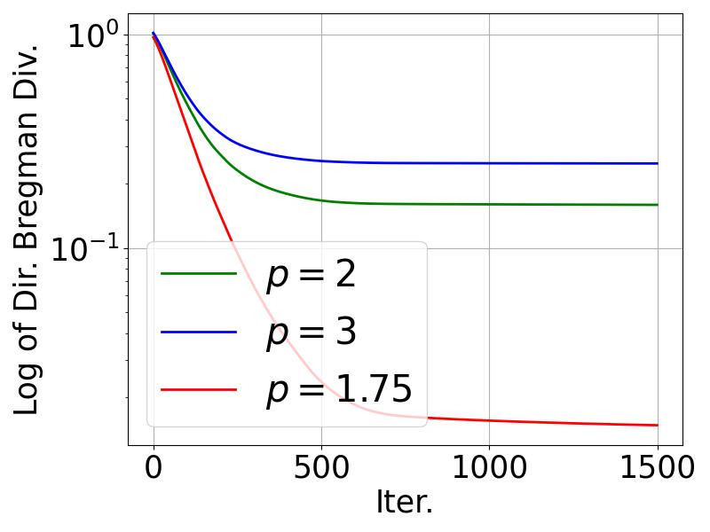
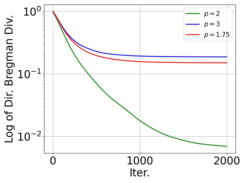
Refer to caption
(a) 1.75\ell_{1.75} Log Divergence
Refer to caption
(b) 2\ell_{2} Log Divergence
Refer to caption
(c) 3\ell_{3} Log Divergence
Figure 13: Graph of the log of directional Bregman divergence between the (a) 1.75\ell_{1.75}, (b) 2\ell_{2}, and (c) 3\ell_{3} optimization paths and the ( ℓ p -AttSVM). This shows how the divergence behaves when viewed from the log-space, adding an extra detail to Figure 4

The model is trained with parameters initialized near the origin, using ℓ p -AttGD with p=1.75,2p=1.75,2, and 33, and a learning rate of 0.10.1. Training lasted for 1,5001,500 epochs for p=1.75p=1.75, 2,0002,000 epochs for p=2p=2, and 20,00020,000 epochs for p=3p=3. Gradients are normalized to accelerate convergence without altering results significantly. We refer to the parameter histories as the 1.75,2,\ell_{1.75},\ell_{2}, and 3\ell_{3} optimization paths. We compute the chosen tokens (αi)i=1n(\alpha_{i})_{i=1}^{n} for the ( ℓ p -AttSVM) problem by selecting the token with the highest softmax probability for each sample. This process is repeated for p=1.75p=1.75, 22, and 33.

G.3 ℓ p -JointGD Experiment

We use the following example dataset for the experiment on joint optimization.

Example 34.

Let n=2n=2, T=3T=3, d=2d=2. Let y1=1y_{1}=1, y2=1y_{2}=-1. Let:

X1=(X11X12X13)=(5.42.42.84.22.60.2),andX2=(X21X22X23)=(0.84.42.20.81.80.2).\displaystyle X_{1}=\begin{pmatrix}X_{11}\\ X_{12}\\ X_{13}\end{pmatrix}=\begin{pmatrix}-5.4&2.4\\ 2.8&4.2\\ 2.6&-0.2\end{pmatrix},\quad\textnormal{and}\quad X_{2}=\begin{pmatrix}X_{21}\\ X_{22}\\ X_{23}\end{pmatrix}=\begin{pmatrix}0.8&-4.4\\ -2.2&-0.8\\ 1.8&0.2\end{pmatrix}. (37)

Let z1=X11z_{1}=X_{11}, z2=X21z_{2}=X_{21}.

We use learning rates 0.10.1 and we trained the model for 1,5001,500 epochs for when p=1.75p=1.75, 2,0002,000 epochs for p=2p=2, and 20,00020,000 epochs for p=3p=3. As it was done in the previous experiment, we obtain the parameter history for each pp, and compute the optimal token for the ( ℓ p -AttSVM) and ℓ p -SVM problems.

G.4 Architecture Details for Stanford Large Movie Review Classification

The model architecture used for semantic analysis on the Stanford Large Movie Review dataset follows the transformer encoder described in 68, with a linear classifier as the final layer.

The embedding layer has trainable token embeddings EE and position encodings PP. The model’s vocabulary size is 30,52230{,}522, with a maximum token length of 512512 and an embedding dimension of 384384. Hence, E30522×384E\in\mathbb{R}^{30522\times 384} and P512×384P\in\mathbb{R}^{512\times 384}. If a token tt is in position ii, its embedding is Xi=Et+PiX_{i}=E_{t}+P_{i}, where EtE_{t} and PiP_{i} denote the ttht^{\text{th}} and ithi^{\text{th}} rows of EE and PP, respectively.

Next, the token features are passed through the encoding blocks, each consisting of a multi-head self-attention layer MultiHead, two layer-normalization layers (LayerNorm1\text{LayerNorm}_{1} and LayerNorm2\text{LayerNorm}_{2}), and a Multilayer Perceptron (MLP). If the sequence of input token features is X1,,XTX_{1},\ldots,X_{T}, and we denote MultiHead(X1,,XT)i\text{MultiHead}(X_{1},\ldots,X_{T})_{i} as the ithi^{\text{th}} token feature from the multi-head self-attention, then the output of the encoding block for the ithi^{\text{th}} token is

LayerNorm2(Xi+MLP(Xi)),\text{LayerNorm}_{2}\bigl(X_{i}^{\prime}+\text{MLP}(X_{i}^{\prime})\bigr),

where

Xi=LayerNorm1(Xi+MultiHead(X1,,XT)i).X_{i}^{\prime}=\text{LayerNorm}_{1}\bigl(X_{i}+\text{MultiHead}(X_{1},\ldots,X_{T})_{i}\bigr).

We apply a dropout rate of 0.20.2 for regularization during training.

The MultiHead attention is a variant of single-head attention that horizontally stacks multiple single-head attentions within the same layer. A single-head attention is equivalent to (2), but with the vector zz replaced by the matrix XX^{\top}, and the vector vv replaced by the matrix VV.

We experimented with 3 encoding blocks (each having 3 attention heads), 4 encoding blocks (with 4 heads), and 6 encoding blocks (with 6 heads). Finally, we pass the feature vector of the first token from the last encoding layer to a linear classifier.

G.5 Additional Experiment with Adam

The ViT architecture that we trained to compare 1.1\ell_{1.1}MD and Adam used a patch size of 44 on the input image, 512512 dimensional token feature, 66 layers of attention blocks with 88 attention heads per attention layer, and a one-layer linear classification layer for the final prediction head on the final [CLS] patch token feature.

The embedding layer of the architecture follows the work of 21, where the embedding layer learns the [CLS] token embedding, a linear map for embedding each image patch, and a positional embedding for each possible position on the image. The details of how the attention layers are implemented are similar to that of the architecture used for the Stanford Large Movie dataset, just that the MLP sublayer is now a two-layer GeLU network, and that we apply the layer normalization before the multihead attention and the MLP instead of after the residual connection. Furthermore, we apply a dropout of 0.10.1 when training the network.

G.6 Addendum to the Attention Map Results

[Uncaptioned image]
Refer to caption
Figure 14: The full attention map table that shows that 1.1\ell_{1.1}-MD provides strictly more attention to the pivotal token compared to 2\ell_{2}-MD, or equivalently GD, for 2222 of the sample sentences. Out of the other 1818 sentences, for 1616 of which, GD strictly outperforms 1.1\ell_{1.1}-MD, while for the other 22, the two algorithms are equally as good.

G.7 Additional Results on Attention Weight Sparsity and Runtime Performance

Refer to caption
(a)
Refer to caption
(b)
Refer to caption
(c)
Refer to caption
(d)
Refer to caption
(e)
Refer to caption
(f)
Refer to caption
(g)
Refer to caption
(h)
Refer to caption
(i)
Figure 15: Histogram of the absolute values of the entries in the WK,WQW_{K},W_{Q}, and WVW_{V} attention weight matrices of the resulting models trained by 1.75,2\ell_{1.75},\ell_{2}, and 3\ell_{3}MD on CIFAR-10.
Refer to caption
(a)
Refer to caption
(b)
Refer to caption
(c)
Refer to caption
(d)
Refer to caption
(e)
Refer to caption
(f)
Refer to caption
(g)
Refer to caption
(h)
Refer to caption
(i)
Figure 16: Histogram of the absolute values of the entries in the WK,WQW_{K},W_{Q}, and WVW_{V} attention weight matrices of the resulting models trained by 1.75,2\ell_{1.75},\ell_{2}, and 3\ell_{3}MD on CIFAR-100.

Similar to the histogram plots for 1.1\ell_{1.1}MD and Adam in Figures 11 and 12 of Section 4.2.2, we plot the histograms for 1.75,2,\ell_{1.75},\ell_{2}, and 3\ell_{3}MD below. As we can see in Figure 15 and 16, the 1.75\ell_{1.75}MD histogram shows a sparser weight distribution than that of Adam and 2\ell_{2}MD, while the 3\ell_{3}MD histogram shows a denser distribution.
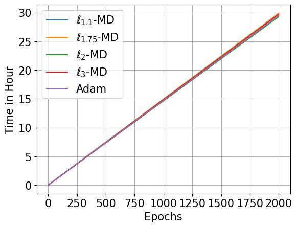
Refer to caption
(a) CIFAR-10 Training Time in Hour
Refer to caption
(b) CIFAR-100 Training Time in Hour
Figure 17: The cumulative time taken to train ViT on CIFAR-10 (left) and CIFAR-100 (right) using p\ell_{p}-MD for p=1.1,1.75,2,p=1.1,1.75,2, and 33 and Adam algorithms across the 2000 epochs. On the left subgraph, it took approximately 29 hours for each of the five optimizers to fully train the model on the CIFAR-10 dataset, and on the right subgraph, it took approximately 25 hours for each of the five optimizers to fully train the model on the CIFAR-100 dataset.

Next, we also take the cumulative time taken to perform each training steps for the experiments in Section 4.2.2. Figure 17 shows that for training CIFAR-10 and CIFAR-100, the differences in the training time between the five different training algorithms are very marginal. Therefore, our algorithms do not have any significant slowdown in the training speed.