Abstract

EEG preprocessing varies widely between studies, but its impact on classification performance remains poorly understood. To address this gap, we analyzed seven experiments with 40 participants drawn from the public ERP CORE dataset. We systematically varied key preprocessing steps, such as filtering, referencing, baseline interval, detrending, and multiple artifact correction steps. Then we performed trial-wise binary classification (i.e., decoding) using neural networks (EEGNet), or time-resolved logistic regressions. Our findings demonstrate that preprocessing choices influenced decoding performance considerably. All artifact correction steps reduced decoding performance across all experiments and models, while higher high-pass filter cutoffs consistently enhanced decoding. For EEGNet, baseline correction further improved performance, and for time-resolved classifiers, linear detrending, and lower low-pass filter cutoffs were beneficial. Other optimal preprocessing choices were specific for each experiment. The current results underline the importance of carefully selecting preprocessing steps for EEG-based decoding. If not corrected, artifacts facilitate decoding but compromise conclusive interpretation.

Introduction

The application of classification models to neural data – known as decoding – has become a standard technique in neurosciences including electroencephalography (EEG) research. Unlike univariate approaches, decoding takes advantage of the multidimensionality of the data, facilitating the exploration of basic research questions or the deployment of brain-computer interfaces. In basic research, decoding can serve as a tool to reduce the multidimensional space spanned by electrode voltages to infer about the neural representational space [1, 2]. On the other hand, BCI studies aim to maximize decoding performance allowing a user or patient to control a machine or to communicate with the environment [3, 4].

Although maximizing decoding performance may not always be the primary goal of a study, it is critical in contexts known to compromise data quality, such as developmental or patient research where motion is common. Maximizing decodeability can be realized at several levels, such as the experimental design, data acquisition, data preprocessing, or the choice of the decoding framework. In the present study, our aim was to illustrate how certain preprocessing choices applied to data derived from common EEG experimental paradigms can increase or decrease decoding performance.

This research question can be addressed in several ways. For example, a many-teams approach (e.g., [5, 6, 7, 8]) can examine the analysis strategies of multiple researchers tackling a set of fixed research questions. Each team thus contributes one analysis pipeline. On the other hand, using a multiverse approach (e.g., [9, 10]) one single team contributes many possible pipelines.

Unlike a many-teams approach that samples an educated subset of individual preprocessing pipelines (i.e., forking paths) from the community, a multiverse approach allows for a grid search over all possible forking paths by systematically varying each predefined preprocessing step. The multiverse approach is not limited to preprocessing pipelines. It can be applied to any analysis step in a study, such as statistical modeling or the selection of a decoder architecture [11, 12].

Similar to previous studies, we constructed a multiverse for EEG preprocessing [9, 10]. However, we did not examine the impact of preprocessing on event-related potential (ERP) amplitude but on decoding performance. To this end, we analyzed several openly available EEG experiments with classifiers derived from two frameworks, a neural network-based classifier (EEGNet, [13]) and a time-resolved logistic regression classifier [14].

Our results demonstrate how preprocessing steps influence decoding performance. Narrow filters increased the decoding performance, especially in a time-resolved framework. In contrast, artifact correction steps generally decreased the decoding performance. We discuss promises and pitfalls in EEG preprocessing with respect to decoding analyses.

Materials and Methods

Datasets

We used the openly available ERP CORE dataset [15] (https://osf.io/thsqg/). $40$ participants underwent six different EEG experiments to identify the following seven ERP components: error-related negativity (ERN), lateralized readiness potential (LRP), auditory oddball-related mismatch negativity (MMN), face-related N170 (N170), visual search-related N2 posterior-contralateral (N2pc), semantics-related N400 (N400), and visual oddball-related P3 (P3) [15]. ERN and LRP were assessed using the same paradigm analyzed differently. EEG was recorded using 30 scalp electrodes (Fig. S1), along with three electrooculogram (EOG) channels, two positioned lateral to the outer canthus of each eye and one below the right eye [15]. For details of the experimental design and paradigms, we refer to Kappenman et al. [15]. We will only address changes to their processing or aspects that seem important for the purposes of this study or its reproduction. In the remainder of this article, we will refer to these experiments by the names of the corresponding components (e.g., MMN, N170, etc., as shown in Table 1).

Data preparation

Data preprocessing and modeling was done using a high-performance computing cluster of the Max Planck Computing & Data Facility (Garching, Germany). Each experiment was preprocessed using MNE (v. 1.5.1) [16] for Python (v. 3.11.6). Triggers from the raw signal were pruned to retain only relevant events (Table 1). Trials of ERN and LRP were analyzed relative to button press, while all other experiments were analyzed relative to stimulus onset (Table 1). Contrary to Kappenman et al. [15], we used a pre-stimulus instead of a pre-response baseline window in the ERN experiment to minimize systematic differences between conditions in the baseline period [17].

Decoding was performed using data from all available scalp electrodes, in contrast to ERP analysis, where it is common practice to analyze data from individual electrodes. Hence, conditions relating to hemisphere, i.e., contralateral & ipsilateral hemisphere, cannot be meaningfully integrated into a whole-brain decoding logic. For this reason, we assigned the trials of some experiments into new conditions for decoding. For LRP decoding, trials were sorted into left and right responses. For N2pc decoding, we sorted trials into left and right targets (Table 1).

Stimulus event times were shifted forward by $26\text{\,}\mathrm{ms}$ to account for the delay of the LCD monitor. Data were downsampled from $1024\text{\,}\mathrm{Hz}$ to $256\text{\,}\mathrm{Hz}$. The raw data channels remained in single-ended mode, so no reference was yet applied. The signal from the two horizontal EOG channels was subtracted to form a single horizontal EOG channel. Similarly, the signal from Fp2 was subtracted from the vertical EOG channel, positioned below the right eye, to form a single vertical EOG channel. The data were then temporarily re-referenced to Cz. The final reference electrode was later determined by the respective forking path. These data then entered the multiverse preprocessing.

-5.5cm0.0cm experiment / paradigm conditions channels component evoked decoding evoked ERN Eriksen flanker task [18] incorrect & correct responses incorrect & correct responses FCz LRP Eriksen flanker task [18] contra- & ipsilateral responses left & right responses C3/C4 MMN passive auditory oddball deviant & frequent sounds deviant & frequent sounds FCz N170 face perception faces & cars faces & cars PO8 N2pc visual search contra- & ipsilateral targets left & right targets PO7/PO8 N400 word pair judgment unrelated & related words unrelated & related words CPz P3 active visual oddball deviant & frequent category deviant & frequent category Pz

Table 1: Properties of the ERP CORE dataset. The experiments are named after the main component, analyzed with the respective paradigm [15]. For each experiment, the conditions and channels used to compute and visualize the ERPs are shown, with the second condition being subtracted from the first condition. For decoding, the trials of experiments LRP and N2pc were assigned to different conditions.

Multiverse preprocessing

All preprocessing steps were restricted to functions included or closely related to the MNE package. Guided by preprocessing steps that were investigated by previous EEG multiverse-like studies [10, 9, 19], we varied ocular artifact correction using independent component analysis (ICA), muscle artifact correction using ICA, low-pass filter (LPF), high-pass filter (HPF), re-referencing, detrending, baseline correction, and artifact correction using autoreject [20, 21]. Figure 1 provides an overview of the different preprocessing steps. A total of $2592$ forking paths resulted from the systematic variation of the chosen preprocessing steps, i.e., the Cartesian product of all preprocessing steps’ options. We chose the same preprocessing steps across all datasets, although the literature suggests a different range of preferred settings depending on the shape of the component. Furthermore, we only included steps that did not require manual intervention by an analyst. Manual intervention is practically not feasible in the multiverse setting and is less consistent, therefore limiting reproducibility [22].

-5.5cm0.0cm

Figure 1: The multiverse of preprocessing choices. By systematically varying each preprocessing step, the raw data was replicated $2592$ times to be preprocessed in unique forking paths. The asterisks indicate processing choices of an example forking path used for some analyses, in which the N170 experiment was re-referenced to the average, and all other experiments were re-referenced to P9/P10.

Theoretically, one could extend the multiverse by additional preprocessing options, such as different methods for ocular artifact correction. However, we decided to limit the number of options for all preprocessing steps to keep the computation time within feasible limits. Furthermore, we did not systematically alter the order of the different preprocessing steps, as this would have led to a combinatorial explosion of forking paths. The selected order roughly followed two previous studies [10, 9], however with ocular and muscle artifact corrections positioned at the beginning to avoid contamination of other preprocessing steps.

For most preprocessing steps, but also for later decoding analysis, we deliberately used the default (hyper-) parameters, if not specified otherwise. Furthermore, we stayed as close as possible at the corresponding tutorials provided from the software packages deployed.

In the following passages, we briefly describe the individual preprocessing steps and their variations in the multiverse.

Ocular artifact correction.

In forking paths including ocular artifact correction, ICA was performed using the corresponding MNE function. First, the raw signal was copied and a $1\text{\,}\mathrm{Hz}$ HPF was applied to the copy. Then an ICA was performed with the picard method, setting the maximum number of iterations to $500$ and estimating $20$ components. The find_bads_eog function with default parameters was used to correlate each component with the artificially generated EOG channels. Components were classified as ocular artifact if passing a threshold based on adaptive $z$-scoring. The ICA solution was then applied to the unfiltered data, effectively subtracting the artifact components from the raw signal.

Muscle artifact correction.

A similar procedure was deployed to that used for ocular artifact correction, using the MNE function find_bads_muscle [23, 24]. In short, three criteria were applied to determine if a component represented a muscle artifact [23, 24], spectral slope, peripherality and spatial smoothness. Because the log-log spectral slope was measured in the range of $7\text{\,}\mathrm{H}\mathrm{z}$ to $45\text{\,}\mathrm{H}\mathrm{z}$, muscle artifact correction was implemented before the LPF. The ICA solution was then applied to the unfiltered data to remove artifactual components.

Filtering.

The default filter function of MNE was applied to all channels of the raw time series, using a linear FIR filter with cutoffs defined in the respective forking paths (Fig. 1). $45\text{\,}\mathrm{Hz}$ was defined as the upper limit for the LPF, since the AC of most countries is typically transmitted at a frequency of $50\text{\,}\mathrm{Hz}$ to $60\text{\,}\mathrm{Hz}$. The LPF of $6\text{\,}\mathrm{Hz}$ was included to exclude alpha activity [25]. The HPF cutoffs were motivated by a range commonly used in EEG literature.

Referencing.

The channels of the raw data were re-referenced to either a single channel (Cz), the average of two channels near the mastoids (P9/P10), or the average of all channels (Fig. 1). According to previous studies, the average of P9 and P10 provided cleaner signals than the commonly used mastoids [15]. Cz or nearby FCz are often used both as an online reference and as a reference during analysis. For convenience, since some of the ERPs of the currently analyzed experiments use FCz as the channel of interest (Table 1), we deployed Cz as reference option in the multiverse. Finally, the average reference is often used to cancel common mode noise and to have a more intuitive interpretation of the topographic distributions of the signals.

Epoching.

Epochs were created for a time window of $1.2\text{\,}\mathrm{s}$ for each experiment (Table S1). This interval included the same interval as the original study [15]. To be able to increase the baseline period in the multiverse, we added $0.2\text{\,}\mathrm{s}$ at the end for ERN and LRP, or added $0.2\text{\,}\mathrm{s}$ at the beginning for all other experiments (Table S1).

Detrending.

In some forking paths, linear detrending was performed prior to baseline correction. When applied, a linear function with intercept and slope was fitted to each epoch and channel using least squares. The signal was detrended by retaining only the corresponding residuals.

Baseline correction.

Baseline correction was applied in a subset of forking paths by first averaging the predefined baseline window in each channel and epoch. The average was then subtracted from the epoch for the respective channel and epoch. The baseline period varied between forking paths (Table S1). If applied, baseline correction was either set to the same $200\text{\,}\mathrm{ms}$ period for each experiment as in Kappenman et al. [15] (but not for ERN), or extended to $400\text{\,}\mathrm{ms}$. Crucially, for some response-locked ERPs such as the ERN, a response-locked baseline window is not optimal, since the conditions (error vs. correct) can already be represented in pre-response components extending into the baseline [17]. Further, systematic differences in reaction time between the two conditions can lead to overlap with different segments of the preceding stimulus ERPs [17]. For this reason, we adjusted the baseline windows to precede the stimulus instead of the response in the ERN experiment (Table S1). Finally, the baseline windows were chosen to end at the same time point within each experiment, resulting in identical post-baseline interval lengths across forking paths (Table S1).

Artifact correction using autoreject.

For further artifact correction on the epochs, the autoreject package (v. 0.4.2) was used in a subset of forking paths [20, 21] (Fig. 1). In short, the package automatically detects and either rejects or interpolates bad sensors and bad trials based on their peak-to-peak voltages. The rejection thresholds were determined by $5$-fold cross-validation. Here we used autoreject in two versions. In the interpolate version, the autoreject hyperparameters were set to values such that all bad sensors were interpolated rather than rejected, ensuring that the resulting number of trials for these forking paths remained identical. The advantage of this approach is, that all trials are kept for later analysis. In the reject version, we provided autoreject with reasonable hyperparameters for consensus ($0.2$, $0.4$, $0.6$, $0.8$) and n_interpolate ($4$, $8$, $16$, $32$). A grid search was performed to find optimal values [20, 21]. If only a few electrodes exceeded the estimated threshold, they were interpolated by neighboring electrodes. If many electrodes exceeded the threshold, the entire epoch was discarded. We used $25\text{\,}\mathrm{\char 37\relax}$ of the epochs to fit the autoreject model.

While the previous preprocessing steps did not change the number of epochs per condition, the second autoreject version could drastically reduce the number of epochs. If a forking path had too few epochs per condition for later cross-validation, the forking path of that participant was discarded. This happened only in rare cases. Note that autoreject shows substantial variability in the number of dropped epochs with different random seeds (Fig. S4 & S5).

Evoked responses

We computed exemplary grand average evoked responses as a proof of principle to ensure that data processing worked as expected. Therefore, for each experiment, we chose a forking path that was related to the preprocessing reported in the original paper releasing the dataset [15]. That is, for all experiments except N170, re-referencing was done on mastoids (average of P9 & P10), with an HPF of $0.1\text{\,}\mathrm{Hz}$, and no LPF applied. ICA was used for both ocular and muscle artifact correction, as well as autoreject in the interpolate version. We chose here to use all artifact correction steps in this example forking path, as the original study performed multiple – including manual – artifact correction steps. The baseline period was $200\text{\,}\mathrm{ms}$ and no detrending was performed. For N170, re-referencing was done using an average reference. The remaining steps were the same as for the other experiments (Fig. 1).

For LRP and N2pc, channels were combined to obtain signals from channels contralateral and ipsilateral to the target (N2pc) or response (LRP) (Table 1). This aggregation was performed only for visualization of evoked responses in accordance with [15], but not for decoding.

Decoding models

We selected a neural network-based and a time-resolved framework for decoding. The former is more commonly used in BCI research [13], whereas the latter is often used in basic research on the time course of category discrimination [26, 27, 25, 28, 29, 30, 31].

Trial-wise decoding using EEGNet

The neural network-based decoding model employed was EEGNet (v. 4) [13], implemented in the braindecode toolbox (v. 0.8) [32, 16]. For each forking path, the preprocessed trials were rescaled using exponential moving standardization. The MMN, P3, and ERN experiments had highly imbalanced classes, while the LRP experiment was only slightly imbalanced. Furthermore, autoreject introduced imbalance when used in the reject version. Therefore, class weights were computed separately for each forking path, experiment, and participant. Next, the order of the trials was shuffled and a stratified $5$-fold cross-validation split was defined. The model was initialized with its default parameters, a batch size of $16$, and the maximum number of epochs (i.e., training cycles, not electrophysiological epochs) was set to $200$. Scoring was performed using balanced accuracy for the $2$-class case. Balanced accuracy is the mean of sensitivity and specificity, and is equivalent to accuracy for class-balanced data. For each cross-validation split, the model was fitted to $\frac{4}{5}$ of the data and evaluated on the remaining $\frac{1}{5}$ of the data. The resulting test accuracies across the $5$ splits were averaged. The approach was repeated for each forking path, experiment, and participant.

Time-resolved decoding using logistic regression

In the literature, raw electrode voltages [25, 29] or averaged pseudo-evoked potentials [30, 31] across trials but for each time point separately are used to train classifiers (Fig. S2). In the present study, we used the raw trials for classification. Data of each time point were standardized by removing the mean and scaling to unit variance. As with EEGNet, balanced accuracy was used for scoring, and class weights were computed individually for each forking path, experiment, and participant. A logistic regression estimator (sklearn v. 1.3.1) was used with a liblinear solver [33] and L2 penalty, applied to each time point with the SlidingEstimator function within MNE. Decoding windows corresponded to the entire trial length (including baseline) and were kept equal in length across experiments, but differed in onset and offset (Table S1). A stratified $10$-fold cross-validation was performed, and the test accuracies were averaged across folds, resulting in one decoding time series for each forking path, experiment, and participant.

The issue of data leakage in EEG decoding

A topic that is closely monitored in the machine learning community, but often neglected in the neuroscience community, is data leakage [34, 35]. Through data leakage, information from the test data is introduced into the training data [36], leading to an overestimation of decoding performance. In our analyses, we used k-fold cross-validations separating training and test epochs. However, the data were jointly preprocessed, leading to imperfect separation. First, the entire time series is used to estimate the ICA solution, meaning segments later assigned to the test set contribute to the removal of components from both the test and training sets. Second, when applying the HPF, test trials can influence training trials due to proximity in the raw time series. Lastly, autoreject involves both training and test data to jointly estimate hyperparameters and rejection thresholds.

One possible solution would be to split the time series into a fixed number of temporally separated segments, the trials of which are then used in different cross-validation folds. Preprocessing operations should then be applied only within each segment. However, many algorithms (e.g., ICA or autoreject) may be less stable when run on less data. A different approach could be a separate preprocessing for each cross-validation fold, so that the training data (e.g., $80\text{\,}\mathrm{\char 37\relax}$) is used to estimate the ICA and autoreject thresholds, and these models are then applied to the test data without separate estimation. However, such a procedure would increase the computation time enormously, and is computationally not feasible in the multiverse. Both approaches would also need precautionary measures in paradigm designs, such as, for instance, an equal distribution of conditions in the different temporarily separated segments. Since we were not interested in the exact test accuracies, but rather in the comparison between test accuracies of different forking paths, we neglected the issue of data leakage in the present study, similar to the majority of previous studies.

Quantification of decoding performance

In the current article, we report only test accuracies, i.e., we use the terms accuracy and decoding accuracy synonymous to test accuracy, as an abbreviation for averaged, cross-validated, balanced test accuracy. We further quantify decoding performance either by test accuracy (EEGNet) or by the $T$-sum of the calculated group statistics (time-resolved).

EEGNet.

For trial-wise decoding using EEGNet, we directly used the averaged, cross-validated, balanced test accuracies. This resulted in up to $2592$ test accuracies for each of the $40$ participants and each of the $7$ experiments. We directly applied a linear mixed model (LMM) (see below), using these test accuracies as the dependent variable.

Time-resolved.

For time-resolved decoding using logistic regression, we first quantified significant clusters at the group level (i.e., across $40$ participants) for each forking path and experiment. This was done using a one-tailed, one-sample permutation cluster mass test [37, 38, 39]. Briefly, we first defined temporal clusters using a cluster forming threshold of $p<0.05$ separately at each time point ($256\text{\,}{\mathrm{s}}^{-1}$) on the zero-centered averaged decoding time series. For each cluster – i.e., union of all neighboring time points above threshold – the sum of $T$-values ($T$-sum) was calculated. Each participant’s individual decoding accuracy time series was then randomly multiplied by either $1$ or $-1$, averaged and zero-centered. Clusters were defined in these permuted datasets using the same cluster forming threshold. By repeating the permutations $1024$ times, we achieved a Monte Carlo sampling of the permutation distribution. The cluster with the highest $T$-sum per iteration was saved for each sample of the permutation distribution. The $p$-value was calculated by relating the $T$-sums of each cluster of the original dataset to those of the sampled permutations, and only clusters falling in the highest $5\text{\,}\mathrm{\char 37\relax}$ quantile were retained. For each forking path and experiment, this procedure corrects the alpha error of a cluster being significant at the family-wise error rate [37]. The $T$-sums over all significant clusters were then entered as the dependent variable into one linear model (LM) per experiment (see below).

As an alternative approach to quantifying time-resolved decoding performance, we averaged the cross-validated test accuracy values across time points after the baseline, for each forking path, experiment, and participant, and entered these values into one LMM per experiment, similar to the procedure applied to EEGNet accuracies. The results are reported in the Supplementary Information. The rationale was that this approach uses accuracy estimates bounded by the interval between $0.5$ and $1.0$, which are more readily interpretable than $T$-sums. However, a typical study would likely rather be focused on delineating and interpreting significant clusters for a group. Therefore, the $T$-sum approach might be practically more relevant and was chosen to be followed in the main manuscript. Estimation of $T$-sums on the individual participant level would also be possible [37] but was avoided for computational reasons in the multiverse context.

Modeling the effects of preprocessing steps

EEGNet

We constructed a LMM for each experiment. The test accuracies per participant and forking path in that experiment served as the dependent variable. All preprocessing steps were modeled as factors. Each step’s version with the smallest intervention served as the reference level (upper option of each step in Figure 1). We also allowed for two-way interactions between all steps. To account for different levels of decoding performance per participant, a random intercept term for the participant was added. To further account for participant-dependent variability within each factor, and to avoid inflation of the alpha error [40, 41], we added random slopes for all main effects and interactions. All LMMs were estimated using MixedModels (v. 4.23.1) for Julia (v. 1.10.2, [42]) and transferred to R [43] for further processing using RCall (v. 0.14.1) and JellyMe4 (v. 1.2.1), and the R package afex (v. 1.3.1, [44]).

Time-resolved

After identifying significant clusters in the decoding time series of each experiment and forking path, we calculated the total $T$-sum across all significant clusters for each experiment and forking path as a proxy for decoding performance. We then constructed one LM for each experiment with the $T$-sum as dependent variable. All single preprocessing steps were modeled as factors, resulting in a full factorial design. As reference-level for each preprocessing step served the variation with the smallest intervention (upper row in Figure 1). Two-way interactions were added between all terms. LMs were estimated using the stats::lm function in base R (v. 4.2.2, [43]).

Modeling interactions

Since preprocessing steps build on each other, they are likely to interact. The recommended way to include interactions is to define the most complete model possible [40]. On the other hand, more model terms make it more difficult to estimate and ultimately interpret the resulting model. We tested whether the addition of interaction terms added value by first testing whether a considerably higher proportion of variance ($R^{2}$) was explained, and second, whether Akaike information criterion (AIC) decreased. Figure S3 shows that a considerable amount of variance is already explained by the main effects when modeling EEGNet decoding performance, but less so for time-resolved decoding performance. Especially for time-resolved decoding performance, interaction terms added substantial value in terms of explained variance (Fig. S3). More importantly, including interactions always decreased AIC values (Fig. S3). To keep the model computationally traceable and the results interpretable, we decided for two limitations regarding model interactions. First, we included only two-way but not higher-order interactions, as the number of model terms (both fixed and random effects) increased drastically. Second, we restricted the model to not estimate the correlations between random effect terms, which significantly shortened the computation time.

Estimation of marginal means

Marginal means and contrasts were estimated using the emmeans package (v. 1.10.0, [45]) in R. Briefly, emmeans extracts the mean responses from statistical models, and returns average response variables – in our case model decoding performance operationalized via accuracy or $T$-sum – for each level of a categorical predictor variable. First, we estimated marginal means for all main (fixed) effects to interpret the influence of each preprocessing choice on model decoding performance. Second, we also estimated marginal means for each interaction effect. This step yielded marginal means for each factor level of a given preprocessing choice, grouped into the factor levels of another preprocessing choice. Similarly, contrasts were computed between all pairs of levels.

Statistical significance was calculated model-wise, i.e., per experiment and decoding framework. For each LMM and LM we applied omnibus $F$-tests to each preprocessing step (main effects and interactions) to determine a significant contribution of the preprocessing step to the decoding accuracy. The Benjamini-Yekutieli procedure was applied to control for the false discovery rate under arbitrary dependence assumptions [46] by separately correcting for the total number of main effects and interactions tested for each experiment. Furthermore, pairwise $T$-ratios and $p$-values were computed for the main effects between the factor levels of each preprocessing step using Tukey adjustment within each preprocessing step [47].

Evaluating the impact of manipulating a single preprocessing step

In an additional analysis, we analyzed the impact of changing one single preprocessing step on decoding performance. For this, we used the example forking path (Fig. 1) as reference. This forking path was defined as reference with the same rational than for the ERP visualization, because it is loosely related to the preprocessing pipeline used in the accompanying article released with the dataset [15]. We then systematically tested, if we manipulated one single processing step, but leave all others unchanged, how decoding performances increases or decreases.

Treatment of statistical significance

We deliberately try not to emphasize statistical significance in the remainder of the manuscript. First, by its very nature, the multiverse could theoretically be inflated by adding more preprocessing choices, either entire steps or variations of steps. If we assume that we add another step with two options, and for simplicity assume no interaction with the previous steps, we effectively doubled the number of forking paths for each group. Thus, small effects could be driven to significance by arbitrarily inflating the multiverse. Second, we used both LMMs (EEGNet) and LMs (time-resolved) to infer the influence of preprocessing steps. Due to the random effects in LMMs and the larger number of data points entering the model (factor $40$), both parameter estimation and the diagnostic performance of the statistical analyses could vary greatly between the two approaches. Third, the dependent variables were different in LMMs and LMs. A reader might be tempted to compare significances of processing steps between EEGNet and time-resolved approaches, which is not possible for the present analyses. For these reasons, we highlight steps that appear important by analyzing the charts rather than only $p$-values.

Results

Evoked responses

Grand average evoked responses were computed for each experiment of the ERP CORE dataset (Fig. 2) using one example forking path, i.e., one particular preprocessing pipeline (Fig. 1). The time courses of the components closely followed the results of the original study (see [15] and their Figure 2), despite differences in preprocessing, the inclusion of all participants, and the lack of manual intervention throughout the preprocessing. The components differed in amplitude between experiments. The ERN and N400 showed the largest amplitudes, whereas LRP, MMN, and N2pc showed rather small amplitudes. Furthermore, the shapes of the components differed, with N400 and P3 covering large time intervals, while, N2pc for example covered only a short time interval.

-5.5cm0.0cm

Figure 2: Grand average evoked responses for each experiment. The data from one example forking path (Fig. 1) were used. The dashed and dotted time courses represent the average responses to each stimulus category. The solid time course represents the difference between the respective categories, illustrating the respective ERP. Time series originate either from a single channel, or from two channels, in which case the mean was calculated. The channel positions are indicated by small graphical legends on the right of each plot. Dotted vertical lines indicate response onset (ERN, LRP), and dashed vertical lines indicate stimulus onset (other experiments). Note that the y-axes are scaled differently for each experiment.

Decoding performance

Decoding was performed separately for each forking path using a neural-network based approach (EEGNet) and a time-resolved approach using logistic regression. For EEGNet, we quantified the (balanced) test accuracies of each forking path – averaged across participants – as a measure of performance (Fig. 3A). For time-resolved decoding, we quantified $T$-sums across participants but within a forking path as a measure of performance (Fig. 3B). Different decoding performances across experiments were observed, with the conditions in ERN being easiest to decode with a median accuracy of roughly $0.85$, followed by LRP, followed by all others, and lastly MMN with a median accuracy of roughly $0.57$. The ranking of the decoding performances was similar for the neural network-based and the time-resolved approaches. When the time-resolved decoding performance was quantified using the average decoding accuracy over a time window instead of the $T$-sum (Fig. S7), the ranking of the experiments remained similar.

High ERP amplitudes at single electrodes were not necessarily associated with high decoding performance across the scalp. For example, LRP showed a rather low amplitude at the selected electrodes (Fig. 2), while the decoding performance was rather high (Fig. 3). Although the two measures are not directly comparable, high amplitudes and long duration of ERPs at one electrode could still facilitate decoding performance across all electrodes, as the data underlying the ERP are also incorporated into the classifier, especially if the high amplitudes are the result of low variability between trials. Furthermore, the ranking not only depends on the magnitude and extent of a component, but also on characteristics of the experimental design, such as the number of stimulus repetitions. Note that the $T$-sum values depend on the data sampling rate, which was held constant between experiments. Therefore, the exact values are rather arbitrary.

-5.5cm0.0cm

Figure 3: Overview of decoding performances. A: EEGNet: Balanced decoding accuracies (y-axis) are plotted for each forking path, averaged across participants, separately for each experiment (x-axis). B: Time-resolved: $T$-sums (y-axis) are plotted for each forking path and across participants, separately for each experiment (x-axis).

Figure 4 illustrates the time-resolved decoding performance of all seven experiments for one single forking path (Fig. 1). Decoding time series revealed large significant clusters, often spanning time windows of over $600\text{\,}\mathrm{ms}$. Peak decoding accuracies were roughly between $0.55$ (MMN) and $0.7$ (ERN). The significant decoding clusters tended to span larger time intervals than the ERPs on selected channels (Fig. 2). Note that exact cluster on- and offsets are not interpretable using the performed cluster mass test [39], as compared to a cluster depth test [48].

-5.5cm0.0cm

Figure 4: Time-resolved decoding accuracy for one forking path. Decoding accuracies are illustrated on the y-axis for each time point (x-axis). The horizontal black line represents chance level. One example forking path was used per experiment (Fig. 1). Decoding was performed within each participant, but the decoding time series were averaged across participants. Different experiments are separated in vertical panels. Dotted vertical lines indicate response onset (ERN, LRP), and dashed vertical lines indicate stimulus onset (remaining experiments). Permutation cluster mass tests with a family-wise error rate correction at $\alpha=0.05$ were performed for each experiment (shaded areas).

Influence of preprocessing choices

For each experiment, we constructed LMMs using EEGNet decoding accuracies or LMs for $T$-sums derived from time-resolved decoding, describing the decoding performance as a function of all preprocessing steps. We then estimated the marginal means for each preprocessing step, i.e., the influence of each choice for a given step on the decoding performance, marginalizing out all other steps. Figure 5 illustrates the marginal means of the main effects for all experiments, both types of decoding models, and for all possible variations of each preprocessing step. The influence – in percent deviation from the marginal mean – of the preprocessing choice on the decoding performance is larger in the time-resolved analysis than in the EEGNet analysis. This is partly due to the deployed $T$-sum metric and the fact that the time-resolved analysis is performed across participants. See Figure S8 for results using average accuracies over time and LMMs for time-resolved decoding.

The impact of most processing steps followed the same direction across experiments (Fig. 5). For example, using artifact correction steps such as ICA or the autoreject package decreased decoding performance in most experiments and decoding frameworks. Furthermore, a high HPF yielded the best decoding performances across experiments and decoding frameworks. In the time-resolved framework, a low LPF further increased decoding performance, while no such trend was observed in the EEGNet framework. The optimal choice of a reference varied between experiments and model types, but its influence was rather weak compared to other preprocessing steps. Linear detrending had a rather positive effect on decoding performance for most experiments and decoding frameworks. Furthermore, a longer time window for baseline correction was beneficial for decoding performance in most experiments. Tables S2 & S3 illustrate results of omnibus $F$-tests for all preprocessing steps, experiments, and model types. In addition, Tables S4 & S5 illustrate the significant pairwise post-hoc tests between factor levels of the main effects.

Two peculiarities emerged, particularly pronounced for EEGNet (Fig. 5A). First, the removal of ocular artifacts was strongly negatively associated with decoding performance in the N2pc experiment. In this experiment, eye movements are expected since the participants might perform involuntary saccades into the visual hemifield of the target, and the target position was decoded (Table 1). Therefore, ocular artifacts are expected to be systematically associated with the class label and thus predictive for the decoder. Accordingly, removing these artifacts reduced decoding performance. Second, removing muscle artifacts was negatively associated with decoding performance, especially in the LRP experiment. In this experiment, left and right hand button presses were decoded (Table 1), and thus systematically different muscle artifacts are expected for the two conditions. These artifacts were predictive and therefore removing them decreased decoding performance.

-5.5cm0.0cm

Figure 5: Influence of preprocessing steps on decoding performance. Percentage deviation from marginal means of either decoding accuracy (EEGNet, A) or $T$-sum (time-resolved, B) are depicted within each tile. Marginal means for each level (x-axis) of preprocessing step (horizontal panels) are normalized to the mean of the respective experiment (vertical panels), and shows the percentage differences in relation to this mean value, and not the absolute improvement or decline in decoding accuracy as a percentage. Color scales differ in A and B. Ocular: ocular artifact correction; muscle: muscle artifact correction; ICA: independent component analysis, low-pass: low-pass filter in Hertz; high-pass: high-pass filter in Hertz; baseline: baseline interval in milliseconds; autoreject version either interpolate (interp) or reject artifact-contaminated trials (reject).

We further analyzed the impact of changing one single preprocessing option at a time compared to the example forking path (Fig. 1) on decoding performance. Figure S9 illustrates, that for most experiments, leaving out artifact correction steps (ICAs, autoreject) increased decoding performance. Similarly, the $6\text{\,}\mathrm{Hz}$ LPFs increased decoding performance in time-resolved decoding. For the other preprocessing steps, a change compared to the reference forking path has different consequences for each experiment. The comparison gives insights only in how a punctual substitution of one (but not more) preprocessing step in the reference forking path impacts decoding performance, and is therefore highly dependent on the reference forking path, which in turn varies largely across researchers [49]. To allow for a simple comparison of individual preprocessing pipelines and their impact on decoding performance, we deployed an online dashboard at https://multiverse.streamlit.app.

We further ranked all forking paths based on their average decoding performance across participants from best (#$1$) to worst (#$2592$), separately for each decoding framework and experiment. Figure S10 illustrates the individual preprocessing choices of the performance-ranked forking paths. In particular, Figure S10 provides more detail on the data points of Figure 3. It turns out that in many experiments analyzed with EEGNet, the best performing forking paths did not include muscle artifact correction. Especially in LRP this effect explains the bimodal distributions seen in Figure 3 by suggesting that all forking paths using muscle artifact correction were ranked lower. Furthermore, for EEGNet the forking paths including autoreject performed rather weakly. For N2pc, the best forking paths did not include ocular artifact correction. For time-resolved decoding, a positive effect of detrending and baseline correction on decoding performance was observed in most experiments.

Interactions between preprocessing choices

We also analyzed two-way interactions between the preprocessing steps. Figure 6 illustrates the interactions related to the N170 experiment within the EEGNet framework as an example. Due to a considerable amount of combinations of experiments and decoding frameworks, we illustrate the remaining interaction results in the Supplementary Information (Fig. S11–S23).

Strong interactions can be observed between HPF and detrending (Fig. 6). In many experiments, applying linear detrending made the choice of the HPF less important, i.e., neutralized an adverse choice regarding the HPF cutoff (Table S2 & S3, Fig. S11–S23). Similarly, for N170 and other experiments, a combination of neither applying HPF nor baseline correction had negative effects on decoding performance.

Several effects can be observed when using autoreject in the version, in which noise-contaminated trials were discarded rather than interpolated. When not applying a HPF, linear detrending or baseline correction but using autoreject in this version, decoding accuracies were lower (Fig. 6 & S10). Presumably, the high electrode voltages – likely present when none of these steps were applied – led to the rejection of many trials, and thus fewer trials were available for model training.

-5.5cm0.0cm

Figure 6: Interactions between preprocessing steps on decoding performance for the N170 experiment and EEGNet decoding. Horizontal and vertical panels illustrate the different preprocessing steps. The individual preprocessing choices are illustrated on the x-axes and color-coded. The color legends on the diagonal refer to each horizontal panel. Marginal means of the decoding accuracies are shown on the y-axes. See Fig. 5 for the definition of abbreviations.

Two pronounced interactions were detected for time-resolved decoding. First, there was an interaction between detrending and baseline correction, with detrending being critical when baseline correction was avoided (Fig. S17–S23). Second, although higher-order interactions were not included in the models, forking paths which included neither baseline correction, detrending, nor HPF showed the worst decoding performance (Fig. S10).

Tables S2 & S3 and the corresponding Figures 6 & S11–S23 illustrate all interaction effects for the other experiments and decoding frameworks. Some interactions were common across experiments, while others could only be observed in single experiments.

Significant clusters in time-resolved decoding

Decoding time series for each forking path and experiment were also visualized individually and ordered according to the total $T$-sum. Figure S24 illustrates the decoding accuracy for each time point that fell within a significant cluster. The peak decoding accuracies were mainly in a similar time window and at a similar amplitude, regardless of the forking path. In most experiments, the extent of the significant clusters remained largely similar for the roughly $90\text{\,}\mathrm{\char 37\relax}$ highest-ranked forking paths (Fig. S24). The significant time windows narrowed down or vanished completely for the $10\text{\,}\mathrm{\char 37\relax}$ lowest-ranked forking paths. Most of the forking paths revealed time windows in which conditions were decoded significantly.

Some decoding time series, especially those corresponding to the well-performing forking paths, showed significant clusters extending into the baseline time window, resulting in a baseline artifact. While a certain percentage of false positives was expected across all forking paths in each experiment, some experiments exhibited a higher amount of spurious decodability, extending into baseline periods. Note that one third of forking paths did not use baseline correction (Fig. 1).

We compared forking paths with and without baseline artifact, and scrutinized the distinctive preprocessing steps of these forking paths. We defined the presence of a baseline artifact when significant clusters occurred within or across the baseline windows (Table S1), except for ERN. For ERN, the baseline was outside the decoding range because it is located before stimulus onset (Table S1). Therefore, we arbitrarily defined clusters emerging before the $0.4\text{\,}\mathrm{ms}$ pre-response time point as problematic, similar to LRP (Table S1). Figure S25 illustrates how many forking paths including a particular version of a preprocessing step led to a baseline artifact in the respective experiment. It turns out that experiments with large ERP components (see Fig. 2) such as ERN, N400, and P3 were more likely to show baseline artifacts when linear detrending was performed beforehand. In addition, a low LPF ($6\text{\,}\mathrm{Hz}$), omitting baseline correction, and in some cases a high HPF ($0.5\text{\,}\mathrm{Hz}$), increased the likelihood of a baseline artifact (Fig. S25).

Influence of the participant

To demonstrate the variability of decoding performance across forking paths (Fig. 3A), we averaged across participants to be consistent with Figure 3B, as $T$-sums were calculated across participants. Without averaging, the variability in accuracy was considerably increased, highlighting a large effect of the participant on decoding accuracy compared to the effect of the forking path (Fig. S6). The remaining variation in decoding performance in each experiment in Figure 3 can be attributed to the choice of the forking path.

We further analyzed whether decoding performance was associated with participant demographics, but did not find an association between age, sex, or handedness and participant-specific decoding performance according to the LMMs’ random intercepts (Fig. S28 & S29). In addition, we correlated the participant-specific random intercepts across experiments, but we only found a significant linear correlation ($r=0.52$, $p=0.011$, false discovery rate-corrected) between LRP and N170 in the EEGNet framework (Fig. S30 & S31). While the participant’s influence on decoding performance is substantial within individual experiments, there is no consistent evidence that the same participant achieves higher decoding accuracy across multiple paradigms.

Discussion

In this study, we investigated the influence of EEG preprocessing steps on decoding performance in two different decoding frameworks. For the neural network-based framework (EEGNet), we compared test accuracies of models fitted to differently preprocessed epochs. For the time-resolved framework, we computed cluster-based permutation statistics on the decoding time series across participants for differently preprocessed epochs and quantified decoding performance as the $T$-sum of the significant clusters. We analyzed seven different experiments separately and modeled the classifier performance as a function of all preprocessing steps.

The results demonstrated, that above chance-level decoding was feasible with most forking paths. For EEGNet, high HPF cutoffs and baseline correction facilitated decoding. For time-resolved classifiers, linear detrending, low LPF cutoffs, and high HPF cutoffs facilitated decoding. All artifact correction steps impaired decoding for all experiments and decoding frameworks. We also found detrimental combinations of processing steps that decreased decoding performance substantially.

Artifacts spuriously enhance decoding performance

Most artifact corrections led to a decrease in decoding performance. This decrease was particularly pronounced in experiments where artifacts can be expected to covary with stimulus categories, such as ocular artifacts in a visual search task and muscle artifacts in a keystroke task. Despite the decrease in performance, removing artifacts should be of interest when model features are to be interpreted spatially or temporally by any technique (e.g., [50, 51, 32]). However, removing artifacts may also remove the neural signal of interest. In some BCI use cases in which the source of the signal may be less relevant, an analyst may even refrain from removing predictive artifacts.

Compared to classical ERP analysis, decoding uses all channels and time points simultaneously to infer differences between conditions [52]. This can lead to a situation in which certain artifacts, while less problematic for ERP analyses in a region of interest, may drive whole-brain decoding and thus inadvertently imply stimulus-related differences. BCI studies have also suggested a drop in decoding performance when various artifact correction methods were applied [53, 54].

Narrow filtering yields high performance

Filter cutoffs also play an important role for decoding performance. Models using data filtered with high HPF and low LPF cutoffs performed best in all experiments using time-resolved decoding. This finding supports using a low LPF cutoff to exclude alpha activity, an influential source of trial-to-trial variability [25]. However, a low LPF cutoff may inflate the time window of an ERP and thus preclude the interpretation of its timing [55]. The same should hold for the temporal interpretation of decoding accuracies. Furthermore, a high HPF cutoff increased decoding performance in both decoding frameworks. HPFs are important for leveling the signal of each epoch, especially when baseline correction has not been performed. However, HPF cutoffs above approximately $0.3\text{\,}\mathrm{Hz}$ also come at a cost, introducing artifacts of opposite polarity before the onset of an ERP [56], which in turn compromise the temporal interpretation of decoding performance. Designing more specified filters can potentially decrease such artifacts [57].

Linear detrending was also positively associated with decoding performance, especially for time-resolved decoding. Before classifier training, the voltage values at each time point and channel were standardized across trials for time-resolved decoding. Random drifts in some electrodes and trials may generate relatively large values – especially at epoch margins – obscuring potentially predictive values of other epochs situated at a much smaller scale at the same electrodes and time points. Only few other decoding studies also removed these remaining drifts from the epochs (e.g., [58]).

Detrimental combinations of preprocessing steps

Unlike previous studies [9, 10], we also allowed for interactions between preprocessing choices. The most common interactions across experiments and decoding frameworks were found between preprocessing steps that level the signal of an epoch to a common range. These include HPF, detrending, and baseline correction. Combining different versions of these steps that do not level the signal to a similar range, i.e., no HPF, no detrending, and no baseline correction, tended to reduce decoding accuracy. Not leveling the signal by means of these preprocessing steps also led to high dropout rates when using autoreject. Furthermore, spurious decodability in baseline periods was observed in many forking paths, leveraged by detrending, a low LPF, and a high HPF. Another study also demonstrated spurious baseline decodability by the combination of of a high HPF, baseline correction, and avoidance of robust detrending [59]. Such effect may also be present in the EEGNet approach, as the baseline was also included in the training of the classifier. We would therefore suggest to also decode from the baseline in the time-resolved framework – and visualize baseline decodability – for the sake of detecting such artifacts. If the baseline period is not decoded in the time-resolved framework, spurious baseline decodability and the likely associated modification in the to-be-interpreted window of the decoding time series might evade detection.

Optimal preprocessing differs for ERPs and decoding

Previous studies using multiverse-like preprocessing have mainly focused on optimal preprocessing with respect to ERP characteristics such as amplitude. For example, a study by Delorme [19] compared preprocessing pipelines and their influence on the number of significant channels between two conditions in three paradigms (Go/No-go task, face perception task, & active auditory oddball task with button press). Their optimal pipeline was dependent on the software used for preprocessing but mainly comprised a HPF and bad channel interpolation. Other steps either reduced the number of significant channels or did not show any effect. In general, across experiments, the optimal HPF was $0.5\text{\,}\mathrm{Hz}$ or higher, similar to our decoding results.

A study by Clayson et al. [10] employed a multiverse to compare the influence of preprocessing on ERP amplitude for two components, ERN and error-related positivity (Pe), using the Eriksen flanker task [18]. For ERN, their optimal processing consisted of a $15\text{\,}\mathrm{Hz}$ LPF and ocular artifact correction with ICA. For Pe, however, their optimal processing in terms of ERP amplitude included a $30\text{\,}\mathrm{Hz}$ LPF, a $0.1\text{\,}\mathrm{Hz}$ HPF, and regression-based ocular artifact correction. Our time window for decoding in the ERN experiment spanned the time windows of both components. We however defined a stimulus-locked rather than a response-locked baseline window. In our search space, the optimal LPF cutoff was at $6\text{\,}\mathrm{Hz}$ for time-resolved decoding. In contrast, for the neural network-based framework, all higher LPF cutoffs ($\geq$$20\text{\,}\mathrm{Hz}$) were equally suitable for decoding. We found the optimal HPF cutoff to be around $0.5\text{\,}\mathrm{Hz}$ in both of our decoding frameworks, while Clayson et al. did not test beyond $0.1\text{\,}\mathrm{Hz}$. Ocular artifact correction played a minor role in decoding, but avoiding this step still resulted in higher decoding performance in our data.

Šoškiç et al. [9] analyzed the influence of preprocessing on the effect magnitude in an N400 experiment. The largest effect was obtained with a HPF between $0.01\text{\,}\mathrm{Hz}$ and $0.1\text{\,}\mathrm{Hz}$ (compared to $1\text{\,}\mathrm{Hz}$) and a mastoid reference (compared to an average reference). We found the same optimal reference for decoding in the N400 experiment for both neural network-based and time-resolved decoding. However, we found that higher HPFs between $0.1\text{\,}\mathrm{Hz}$ and $0.5\text{\,}\mathrm{Hz}$ lead to higher accuracies.

Generalizability of the insights from the multiverse

Some of the observed effects of preprocessing on decoding were generalizable across experiments, such as the optimal LPF cutoff (time-resolved), baseline correction (EEGNet), or detrending (time-resolved). Some effects were even generalizable across decoding frameworks, such as the optimal HPF cutoff, or the negative effect of any artifact correction step.

The generalizability of the results to different decoding frameworks remains to be demonstrated in the future. We deliberately used two different decoding frameworks to show similarities and differences regarding the influence of preprocessing using multiverse analyses. However, even changing the decoding model – e.g., to support vector machines in a time-resolved framework, or to different neural networks instead of EEGNet – could change the multiverse results. Decoder hyperparameter optimization may also change the optimal preprocessing choices, but this topic is beyond the scope of the current study. Instead, we used default hyperparameters. Decoder hyperparameter optimization could be added to the multiverse, as could the choice of the decoding model itself be added. One could even treat the multiverse for preprocessing as a kind of grid search-like hyperparameter optimization, if cross-validated and applied to independent test data.

The experiments used in the present study were tailored to ERP-related research questions. ERPs have marked voltage differences in defined channels and time windows, which are likely to also become predictive in decoding. Moreover, the influence of the forking path might be larger if, for example, the experiments included fewer repetitions per stimulus category. Good decoding performance was expected for the well-replicated effects studied here.

However, different kinds of EEG paradigms need different decoding frameworks. For example, for experiments in which the spectral power differences between conditions are analyzed [60, 61], a decoding framework tailored to frequency decoding is more suited [32].

Recent experiments are often based on the rapid serial visual presentation (RSVP) structure [62, 63, 64], in which many different object categories are presented in quick succession to run a large number of trials per object category. These experiments, also employed in the auditory domain [65, 66], are not directly designed to find well-described ERPs. Instead, the literature describes ERPs only for a small subset of the contrasts that can be constructed between categories included in an RSVP experiment. For example, faces can usually be easily distinguished from other categories in decoding based on the data underlying the N170, but also information from other channels not typically used in characterizing the N170. However, differences between other categories (e.g., computers and cars) are less well-described. A possible explanation is that the differentiation of these categories had little evolutionary relevance, leading to idiosyncratic representation for each participant rather than a systematic and generalizable representation across participants. More dense electrode coverage might be helpful to find such subtle differences between categories. From this point of view, the decoding accuracies shown in the present N170 experiment presumably represent the upper limit of decoding accuracies at the given number of stimulus repetitions, due to the strong nature of the N170 component. Other contrasts might lead to classifiers with lower accuracy. Importantly, one should not extrapolate the present recommendations based on the multiverse results regarding the N170 experiment – the only object categorization experiment analyzed in the present study – to an RSVP experiment. The reason is that the preprocessing would then be optimized for the face vs. car contrast, but not for the many other contrasts between categories. In fact, any preprocessing prior to multi-class decoding could bias decodability by filtering out the predictive features of one class represented in a particular frequency spectrum. From this perspective, using the data in a rather raw (i.e., not preprocessed) form might be favorable, given that the classifier works well with it.

Finally, the multiverse also illustrates the challenge of analytical variability with regard to preprocessing. Although only a subset of possible forking paths would be practically used by an analyst, the variability is still substantial [49], offering an analyst sufficient degrees of freedom for potential malpractice. Preregistration should be one important building block to increase transparency and avoid the potential for malpractice [67, 68].

Inflating the multiverse

The constructed multiverse naturally included only a limited subset of preprocessing steps and variations. One could have added any number of additional variations of each analysis step. For example, one could have sampled the filter cutoffs more densely to find a better optimum, rather than just an optimum based on the available choices. Furthermore, a large number of plausible methods have been published for each artifact correction step, such as regression-based methods for ocular artifact correction [69], trial-masked robust detrending [59], or robust averaging [70], to name a few. For this reason, we have made some simple but reasonable choices, e.g., ICA for ocular artifact correction, for each step that were readily available in the MNE package. It remains to be seen whether these choices could generalize to similar approaches, other software, and other package versions.

Besides the exact steps performed, previous studies also vary widely in their order of preprocessing steps [5]. Systematically varying the order of the steps however leads to a combinatorial explosion, complicating both computation and interpretation. Furthermore, the interpretation of interactions between preprocessing steps changes depending on their order. Accordingly, such a study needs to be conducted in the future. We have tested one alternative multiverse with a slightly different order of steps, i.e., (1) re-referencing, (2) HPF & LPF, (3) ocular artifact correction, (4) muscle artifact correction, (5) baseline correction & detrending, and (6) autoreject (Fig. S26 & S27). Most effects were qualitatively similar to those presented in the main manuscript.

Conclusion

In the present study, we systematically varied a wide range of EEG preprocessing steps to evaluate their impact on decoding performance. For EEGNet decoding, high high-pass filter cutoffs and baseline correction improved decoding performance, whereas for time-resolved decoding, high high-pass filter cutoffs, low low-pass filter cutoffs, and linear detrending improved decoding. Importantly, all artifact removal steps decreased decoding performance. Optimal choices for other preprocessing steps varied depending on the experimental paradigm. We suggest to carefully select EEG preprocessing steps for decoding, as selecting steps that maximize decoding performance is associated with limitations in downstream feature interpretability.

Data & code availability

A GitHub repository containing all scripts is available at https://github.com/kesslerr/m4d, including Bash- & Python scripts handling the complete multiverse preprocessing and decoding on a high-performance computing cluster. The repository also comprises all scripts to compute LMMs in Julia, and to perform all remaining analyses in R based on a targets pipeline [71]. To allow for a simple comparison of individual preprocessing pipelines and their impact on decoding performance, we deployed an online dashboard at https://multiverse.streamlit.app. The raw dataset used in our analyses is shared by its authors [15] at https://osf.io/thsqg/.

Author contributions

Conceptualization: RK, AE; Data curation: RK; Formal analysis: RK; Funding acquisition: MAS; Investigation: RK; Methodology: RK, AE; Resources: RK, MAS; Software: RK; Visualization: RK; Writing – original draft: RK; Writing – review & editing: AE, MAS.

Supplementary Information

1. Supplementary methods
2. Variability due to random seed in autoreject
3. Supplementary results on decoding performance
4. Statistical results on main effects and interactions
5. Interaction plots
6. Time-resolved accuracy and baseline artifact
7. Alternative order of preprocessing steps
8. Influence of the participant in the

Supplementary methods

Figure S1: Schematic of the EEG montage. $30$ scalp electrodes were recorded along with three EOG electrodes (not shown).

-5.5cm0.0cm

Table S1: Epoching. Time-locking events, epoch intervals, and baseline reference and intervals. The total duration of the epochs is kept equal across experiments. The baseline interval varied per forking path, either not applied, or a window of $200\text{\,}\mathrm{ms}$ or $400\text{\,}\mathrm{ms}$. The illustrated baseline intervals are with respect to the baseline reference. The illustrated epoch intervals are with respect to the time-locking event. The length of the entire trials and the post-baseline time windows was kept equal between forking paths.

experiment /	time-locking event	epoch interval [ms]	baseline reference	baseline interval [ms]
component				$200\text{\,}\mathrm{ms}$	$400\text{\,}\mathrm{ms}$
ERN	response	$(-600;600)$	stimulus	$(-200;0)$	$(-400;0)$
LRP	response	$(-800;400)$	response	$(-600;-400)$	$(-800;-400)$
MMN	stimulus	$(-400;800)$	stimulus	$(-200;0)$	$(-400;0)$
N170	stimulus	$(-400;800)$	stimulus	$(-200;0)$	$(-400;0)$
N2pc	stimulus	$(-400;800)$	stimulus	$(-200;0)$	$(-400;0)$
N400	stimulus	$(-400;800)$	stimulus	$(-200;0)$	$(-400;0)$
P3	stimulus	$(-400;800)$	stimulus	$(-200;0)$	$(-400;0)$

Figure S2: Schematic of time-resolved decoding. In time-resolved decoding analysis, all channel values (here, electrode voltages) from all trials at each respective time point are used to train and test binary classifiers (top panel). In the present study, logistic regressions were used. The (cross-validated, balanced) test accuracies are then written into a decoding time series (lower panel), which is further analyzed across participants.

Figure S3: AIC and $R^{2}$ values for models without interactions and models with two-way interactions included. Including interaction terms consistently decreased AIC values, supporting the decision to include these terms in our model. The $R^{2}$ values from EEGNet compared to time-resolved models were already high without interaction values, indicating that a large fraction of variance is already explained by the main effects.

Variability due to random seed in autoreject

The autoreject package [20, 21] shows considerable variability in the number of dropped epochs, when applied to the same data but using a different random seed. To illustrate this, we used one example participant in the ERN experiment to show the influences of (1) the random seed in the autoreject function, and (2) a random seed in trial sampling prior to fitting the autoreject model. Some variability due to the seed in sampling the epochs for fitting autoreject is expected. We therefore tested $19$ random seeds at both stages. Figure S4 illustrates, that substantial variability is introduced by random seeds at both stages. However, Figure S5 illustrates, that similar epochs are rejected for different seeds, i.e., if a seed rejects more epochs, it usually contains epochs also rejected using a different seed.

-5.5cm0.0cm

Figure S4: Fraction of maintained epochs for different seeds. The fraction of maintained epochs (x-axes) for different random seeds are counted across seeds (y-axes). Upper panel: Seed varied in autoreject function. Lower panel: Seed varied in epoch sampling.

-5.5cm0.0cm

Figure S5: Rejected epochs for different seeds. For each epoch (x-axes) and random seed (y-axes), black tiles indicate rejection of an epoch due to exceeding the estimated threshold, whereas white tiles indicate epochs which were maintained. Upper panel: Seed varied in autoreject function. Lower panel: Seed varied in epoch sampling.

Supplementary results on decoding performance

Figure S6: Overview of EEGNet decoding accuracies. (Balanced) Decoding accuracies (y-axis) are illustrated for each forking path and participant, separately for each experiment (x-axis). Contrary to Figure 3A, no averaging across participants was performed for each forking path. One can observe the higher variability in decoding accuracy when not removing the participant variability compared to Figure 3A.

Figure S7: Overview of average time-resolved decoding accuracies. Average post-baseline decoding accuracies (y-axis) are plotted for each forking path, further averaged across participants, separately for each experiment (x-axis). Unlike Figure 3B, it is the average decoding accuracy that is plotted, not the $T$-sum.

-5.5cm0.0cm

Figure S8: Influence of preprocessing steps on time-resolved decoding performance. The average post-baseline decoding accuracy is used as a proxy for decoding performance instead of $T$-sum. See Figure 5 for more details.

-5.5cm0.0cm

Figure S9: Influence of varying one single preprocessing steps on decoding performance. Absolute increase or decrease in decoding performance – either accuracy (EEGNet, A) or $T$-sum (time-resolved, B) – is depicted within each tile. Change in decoding performance for each level (x-axis) of preprocessing step (horizontal panels) are illustrated in comparison to the example forking path (Fig. 1) for each respective experiment (vertical panels). Color scales differ in A and B. See Figure 5 for details.

-5.5cm0.0cm

Figure S10: Ranked forking path performances. For each decoding framework (EEGNet: A, time-resolved: B) and experiment (horizontal panels), the forking paths were ranked from best (#$1$) to worst (#$2592$). The individual variations of each preprocessing step (x-axes) are color-coded. Each individual row corresponds to one data point in Figure 3. Ocular: ocular artifact correction; muscle: muscle artifact correction; ICA: independent component analysis, low-pass: low-pass filter in Hertz; high-pass: high-pass filter in Hertz; baseline: baseline interval in milliseconds; autoreject version either interpolate (interp) or reject artifact-contaminated trials (reject).

Statistical results on main effects and interactions

-5.5cm0.0cm model term ERN LRP MMN N170 N2pc N400 P3 ocular muscle *** . low-pass ** high-pass * *** * reference . * detrending * . ** baseline *** *** *** ** *** autoreject ** *** *** . *** ocular:muscle ocular:low-pass ocular:high-pass ocular:reference ocular:detrending ocular:baseline ocular:autoreject * muscle:low-pass * . muscle:high-pass muscle:reference muscle:detrending muscle:baseline muscle:autoreject low-pass:high-pass * low-pass:reference low-pass:detrending ** . low-pass:baseline low-pass:autoreject high-pass:reference . high-pass:detrending *** . *** *** *** high-pass:baseline *** *** *** *** *** high-pass:autoreject ** *** *** *** *** *** reference:detrending reference:baseline reference:autoreject ** . detrending:baseline ** *** *** *** *** *** detrending:autoreject *** . *** *** ** baseline:autoreject *** *** *** *** ***

Table S2: Significant effects of preprocessing on EEGNet decoding performance, separately for each experiment. $F$-tests were performed for each processing step. Stars indicate the signicifance level (’.’ $p<0.1$; ’*’ $p<0.05$; ’**’ $p<0.01$; ’***’ $p<0.001$), false discovery rate-corrected using the Benjamini–Yekutieli procedure. Ocular: ocular artifact correction; muscle: muscle artifact correction; ICA: independent component analysis, low-pass: low-pass filter; high-pass: high-pass filter.

-5.5cm0.0cm model term ERN LRP MMN N170 N2pc N400 P3 ocular *** *** . *** *** *** muscle *** *** *** *** *** *** *** low-pass *** *** *** *** *** *** *** high-pass *** *** *** *** *** *** *** reference *** * *** *** *** detrending *** *** *** *** *** *** *** baseline *** *** *** *** *** *** *** autoreject *** *** *** *** *** *** *** ocular:muscle ** *** * ocular:low-pass ocular:high-pass ocular:reference ocular:detrending *** *** ocular:baseline ocular:autoreject muscle:low-pass *** *** *** *** muscle:high-pass *** *** ** ** * muscle:reference *** * muscle:detrending *** *** *** *** muscle:baseline ** muscle:autoreject . *** low-pass:high-pass *** *** *** *** ** ** low-pass:reference low-pass:detrending ** *** *** *** *** *** *** low-pass:baseline *** *** *** *** *** *** low-pass:autoreject *** . high-pass:reference *** high-pass:detrending *** *** *** *** *** *** *** high-pass:baseline * *** *** *** *** *** *** high-pass:autoreject *** *** *** ** *** reference:detrending . . reference:baseline *** reference:autoreject *** detrending:baseline *** *** *** *** *** *** *** detrending:autoreject ** *** ** *** baseline:autoreject *** ** *** ***

Table S3: Significant effects of preprocessing on time-resolved decoding performance, separately for each experiment. See Table S2 for details.

-5.5cm0.0cm variable level.1 level.2 ERN LRP MMN N170 N2pc N400 P3 ocular None ICA * muscle None ICA *** ** * . low-pass None 6 Hz . *** low-pass None 20 Hz low-pass None 45 Hz low-pass 6 Hz 20 Hz * *** low-pass 6 Hz 45 Hz * *** low-pass 20 Hz 45 Hz high-pass None 0.1 Hz . ** * high-pass None 0.5 Hz ** *** . * high-pass 0.1 Hz 0.5 Hz reference average Cz ** * reference average P9/P10 * . * * reference Cz P9/P10 * detrending None linear ** ** *** baseline None 200 ms *** ** *** * ** baseline None 400 ms *** *** *** ** *** baseline 200 ms 400 ms autoreject None interpolate ** *** * *** . *** autoreject None reject ** *** ** * * autoreject interpolate reject

Table S4: For each experiment, pairwise post-hoc comparisons in EEGNet decoding performance within each preprocessing step using Tukey adjustment. See Table S2 for details.

-5.5cm0.0cm variable level.1 level.2 ERN LRP MMN N170 N2pc N400 P3 ocular None ICA *** *** ** *** *** *** muscle None ICA *** *** *** *** *** *** *** low-pass None 6 Hz *** *** *** *** *** *** *** low-pass None 20 Hz *** *** *** *** *** *** *** low-pass None 45 Hz ** *** *** *** *** *** *** low-pass 6 Hz 20 Hz *** *** *** *** *** *** *** low-pass 6 Hz 45 Hz *** *** *** *** *** *** *** low-pass 20 Hz 45 Hz ** *** *** *** *** *** *** high-pass None 0.1 Hz *** *** *** *** *** *** *** high-pass None 0.5 Hz *** *** *** *** *** *** *** high-pass 0.1 Hz 0.5 Hz *** *** *** *** *** reference average Cz *** . *** * reference average P9/P10 . *** ** *** *** *** reference Cz P9/P10 *** * detrending None linear *** *** *** *** *** *** *** baseline None 200 ms *** ** *** *** *** baseline None 400 ms *** *** *** *** *** *** *** baseline 200 ms 400 ms *** *** *** *** *** *** autoreject None interpolate *** *** *** *** *** *** *** autoreject None reject *** *** *** *** *** *** autoreject interpolate reject *** *** ** *** *** ***

Table S5: For each experiment, pairwise post-hoc comparisons in time-resolved decoding performance within each preprocessing step using Tukey adjustment. See Table S2 for details.

Interaction plots

-5.5cm0.0cm

Figure S11: Interactions between preprocessing steps on decoding performance for ERN and EEGNet decoding. See Figure 6 for details.

-5.5cm0.0cm

Figure S12: Interactions between preprocessing steps on decoding performance for LRP and EEGNet decoding. See Figure 6 for details.

-5.5cm0.0cm

Figure S13: Interactions between preprocessing steps on decoding performance for MMN and EEGNet decoding. See Figure 6 for details.

-5.5cm0.0cm

Figure S14: Interactions between preprocessing steps on decoding performance for N2pc and EEGNet decoding. See Figure 6 for details.

-5.5cm0.0cm

Figure S15: Interactions between preprocessing steps on decoding performance for N400 and EEGNet decoding. See Figure 6 for details.

-5.5cm0.0cm

Figure S16: Interactions between preprocessing steps on decoding performance for P3 and EEGNet decoding. See Figure 6 for details.

-5.5cm0.0cm

Figure S17: Interactions between preprocessing steps on decoding performance for ERN and time-resolved decoding. See Figure 6 for details.

-5.5cm0.0cm

Figure S18: Interactions between preprocessing steps on decoding performance for LRP and time-resolved decoding. See Figure 6 for details.

-5.5cm0.0cm

Figure S19: Interactions between preprocessing steps on decoding performance for MMN and time-resolved decoding. See Figure 6 for details.

-5.5cm0.0cm

Figure S20: Interactions between preprocessing steps on decoding performance for N170 and time-resolved decoding. See Figure 6 for details.

-5.5cm0.0cm

Figure S21: Interactions between preprocessing steps on decoding performance for N2pc and time-resolved decoding. See Figure 6 for details.

-5.5cm0.0cm

Figure S22: Interactions between preprocessing steps on decoding performance for N400 and time-resolved decoding. See Figure 6 for details.

-5.5cm0.0cm

Figure S23: Interactions between preprocessing steps on decoding performance for P3 and time-resolved decoding. See Figure 6 for details.

Time-resolved accuracy and baseline artifact

-5.5cm0.0cm

Figure S24: Time-resolved decoding accuracy for all forking paths. The decoding accuracy for each time point (x-axes) is color-coded. The forking paths of each experiment (horizontal panels) are ranked based on their $T$-sum from #$1$ (best) to #$2592$ (worst) on the y-axes, and therefore correspond to the forking paths of Figure S10 (bottom). The vertical aquamarine line illustrates stimulus or response onset (Table S1). Only time points are color-coded, which fall in a significant cluster as defined by cluster-permutation testing.

-5.5cm0.0cm

Figure S25: Influence of preprocessing steps on the presence or absence of a baseline artifact in time-resolved decoding. For each experiment (vertical panels) and preprocessing step (horizontal panels) and its respective version (x-axes), the number of forking paths producing a so-called baseline artifact during time-resolved decoding is counted (y-axes). Green bars illustrate the number of forking paths without such an artifact, and red bars the number of forking paths with such an artifact.

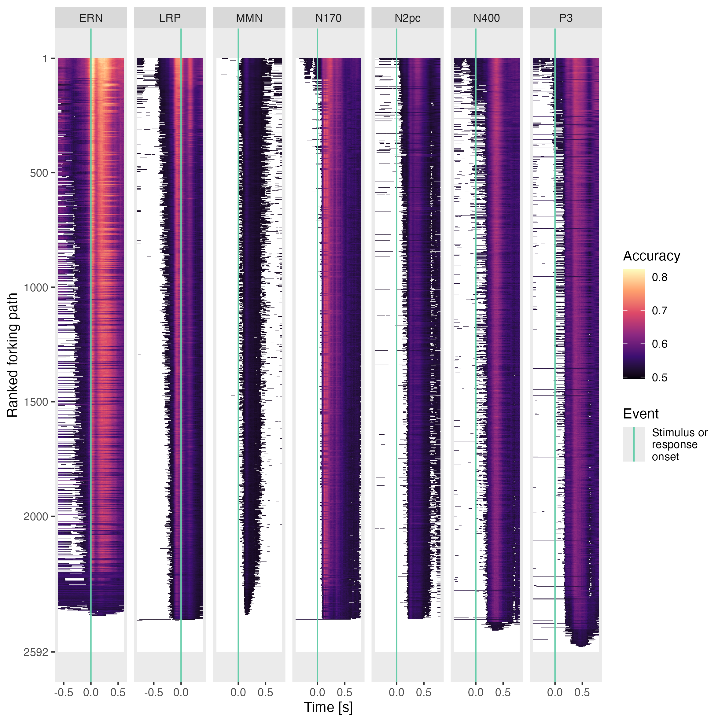
Alternative order of preprocessing steps

We tested one alternative order of preprocessing steps in a reduced multiverse. There we applied the steps in the order of (1) re-referencing, (2) HPF & LPF, (3) ocular artifact correction, (4) muscle artifact correction, (5) baseline correction & detrending, and (6) autoreject. In this version, we always performed a baseline correction (either $200\text{\,}\mathrm{ms}$ or $400\text{\,}\mathrm{m}\mathrm{s}$). For detrending, we chose between offset (subtract mean) and linear (apply linear function and keep residuals). We either used autoreject in the interpolate version, or did not apply it. The remaining choices were the same.

Figure S26 illustrates the decoding performances (accuracies and $T$-sums) for classifiers trained on data preprocessed with the alternative multiverse order. The magnitudes were comparable to those reported in our main multiverse pipeline (Fig. 3). We also computed the corresponding marginal means (Fig. S27). Most effects were in a similar direction as in our main multiverse results (Fig. 5). However, the LPF in the EEGNet framework had quite opposite effects. This can be explained by the fact that it is followed by the muscle artifact correction step, which had no effect (i.e., did not drop any components) when a LPF of $6\text{\,}\mathrm{Hz}$ or $20\text{\,}\mathrm{Hz}$ was applied. This, in turn, resulted in all forking paths with these filter settings having no muscle artifacts removed, which in turn were predictive and increased decoding performance.

-5.5cm0.0cm

Figure S26: Overview of decoding performances in an alternative multiverse. A: (Balanced) Decoding accuracies (y-axis) are plotted for each forking path (averaged across participants), separately for each experiment (x-axis). B: $T$-sums (y-axis) are plotted for each forking path and across participants, separately for each experiment (x-axis).

-5.5cm0.0cm

Figure S27: Influence of preprocessing steps on decoding performance in an alternative multiverse. Percentage deviation from marginal means of either decoding accuracy (EEGNet, A) or $T$-sum (time-resolved, B) are depicted within each tile. Marginal means for each level (x-axis) of preprocessing step (horizontal panels) are normalized to the mean of the respective experiment (vertical panels)). Each tile therefore shows the percentage differences in relation to this mean value. Color scales differ in A and B. The horizontal panels are ordered according to the preprocessing steps in the pipeline. The order differs with respect to Figure 5. See Figure 5 for details.

Influence of the participant in the LMMs

Within the LMMs constructed to explain the accuracies of trained EEGNet models, we included random intercepts for the $40$ participants. Figure S28 illustrates, how the distribution of age, sex, handedness corresponds to the random intercept, i.e., to the individual participants offset in decoding accuracy. Age and handedness did not show any noticeable pattern. We further tested the difference of random intercepts between sexes using a Mann–Whitney $U$ test with Benjamini Hochberg false discovery rate adjustment [72] for $7$ experiments (Fig. S28, middle column). No significant differences were observed. We repeated the same analysis for time-resolved LMM results, which were fitted with the averaged decoding accuracies over time as dependent variables (Fig. S29). No significant differences were observed.

-5.5cm0.0cm

Figure S28: Relation between random intercepts and participant demographics using EEGNet. For each experiment (row), each participant’s random intercept – i.e., the individual offset in decoding accuracy – are plotted against demographic variables. Left column: The relationship between age and random intercept, grouped by sex (red=female, green=male). Middle column: The association between sex and random intercept. $P$-values represent the results of a false discovery rate-corrected Man-Whitney $U$ test using the Benjamini Hochberg adjustment. No association was significant. Right column: Histogram of the relationship between random intercept and handedness. Only two participants in the dataset were left-handed.

-5.5cm0.0cm

Figure S29: Relation between random intercepts and participant demographics using time-resolved decoding. See Figure S28 for details. No association was significant.

In addition, Figure S30 illustrates the estimated random intercepts for each participant across the $7$ experiments. One might hypothesize that participants with a high random intercept in one experiment would also have a high random intercept in the other experiments, indicating that it is easier to decode of EEG signals from some participants, but not others. For each pair of experiments, we computed Pearson correlation coefficients between the random intercepts of the same participants, and corrected for the false discovery rate using Benjamini Hochberg procedure. Figure S30 generally shows no such a relationship. The only significant correlations were observed between the random intercepts of LRP and N170 (Fig. S30). We repeated the same analysis for time-resolved LMM results, which were fitted with the averaged decoding accuracies over time as dependent variables (Fig. S31). No significant correlations were observed.

Figure S30: Correlations of random intercepts between experiments (EEGNet decoding). Pairwise Pearson correlations were computed, correlating the random intercepts of the same participants but in two different experiments and therefore extracted from two different LMMs. The lower diagonal illustrates the random intercepts of the same participants but across two experiments and LMMs, extracted from these LMMs. The on-diagonal elements show a kernel density estimate of the distributions. The upper diagonal illustrates the Pearson correlation coefficients and associated false discovery rate-corrected $p$-values.

Figure S31: Correlations of random intercepts between experiments (time-resolved decoding). See Figure S30 for details.

References

- 1. N. Kriegeskorte, M. Mur and P. Bandettini. Representational similarity analysis – connecting the branches of systems neuroscience. Frontiers in Systems Neuroscience, 2008.
- 2. J. V. Haxby, A. C. Connolly and J. S. Guntupalli. Decoding Neural Representational Spaces Using Multivariate Pattern Analysis. Annual Review of Neuroscience, 37(1), 2014.
- 3. S. Aggarwal and N. Chugh. Review of Machine Learning Techniques for EEG Based Brain Computer Interface. Archives of Computational Methods in Engineering, 29(5), 2022.
- 4. J. Pan, Y. Li, Z. Gu and Z. Yu. A comparison study of two P300 speller paradigms for brain–computer interface. Cognitive Neurodynamics, 7(6), 2013.
- 5. Y. G. Pavlov, N. Adamian, S. Appelhoff, M. Arvaneh, C. S. Benwell et al. #EEGManyLabs: Investigating the replicability of influential EEG experiments. Cortex, 144, 2021.
- 6. D. Trübutschek, Y.-F. Yang, C. Gianelli, E. Cesnaite, N. L. Fischer et al. EEGManyPipelines: A Large-scale, Grassroots Multi-analyst Study of Electroencephalography Analysis Practices in the Wild. Journal of Cognitive Neuroscience, 36(2), 2024.
- 7. R. Botvinik-Nezer, F. Holzmeister, C. F. Camerer, A. Dreber, J. Huber et al. Variability in the analysis of a single neuroimaging dataset by many teams. Nature, 582(7810), 2020.
- 8. M. A. Yücel, R. Luke, R. C. Mesquita, A. Von Lühmann, D. M. A. Mehler et al. The fNIRS Reproducibility Study Hub (FRESH): Exploring Variability and Enhancing Transparency in fNIRS Neuroimaging Research, 2024. MetaArXiv. Available at: https://osf.io/pc6x8.
- 9. A. Šoškić, S. J. Styles, E. S. Kappenman and V. Kovic. Garden of forking paths in ERP research – effects of varying pre-processing and analysis steps in an N400 experiment, 2022. PsyArXiv. Available at: https://osf.io/8rjah.
- 10. P. E. Clayson, S. A. Baldwin, H. A. Rocha and M. J. Larson. The data-processing multiverse of event-related potentials (ERPs): A roadmap for the optimization and standardization of ERP processing and reduction pipelines. NeuroImage, 245, 2021.
- 11. G. G. Cantone and V. Tomaselli. Theory and methods of the multiverse: an application for panel-based models. Quality & Quantity, 58(2), 2024.
- 12. M. Del Giudice and S. W. Gangestad. A Traveler’s Guide to the Multiverse: Promises, Pitfalls, and a Framework for the Evaluation of Analytic Decisions. Advances in Methods and Practices in Psychological Science, 4(1), 2021.
- 13. V. J. Lawhern, A. J. Solon, N. R. Waytowich, S. M. Gordon, C. P. Hung and B. J. Lance. EEGNet: a compact convolutional neural network for EEG-based brain–computer interfaces. Journal of Neural Engineering, 15(5), 2018.
- 14. A. Gramfort, M. Luessi, E. Larson, D. A. Engemann, D. Strohmeier et al. MNE software for processing MEG and EEG data. NeuroImage, 86, 2014.
- 15. E. S. Kappenman, J. L. Farrens, W. Zhang, A. X. Stewart and S. J. Luck. ERP CORE: An open resource for human event-related potential research. NeuroImage, 225, 2021.
- 16. A. Gramfort, M. Luessi, E. Larson, D. A. Engemann, D. Strohmeier et al. MEG and EEG data analysis with MNE-Python. Frontiers in Neuroscience, 7, 2013.
- 17. D. Feuerriegel and S. Bode. Bring a map when exploring the ERP data processing multiverse: A commentary on Clayson et al. 2021. NeuroImage, 259, 2022.
- 18. B. A. Eriksen and C. W. Eriksen. Effects of noise letters upon the identification of a target letter in a nonsearch task. Perception & Psychophysics, 16(1), 1974.
- 19. A. Delorme. EEG is better left alone. Scientific Reports, 13(1), 2023.
- 20. M. Jas, D. Engemann, F. Raimondo, Y. Bekhti and A. Gramfort. Automated rejection and repair of bad trials in MEG/EEG. In 6th International Workshop on Pattern Recognition in Neuroimaging (PRNI), Trento, Italy, 2016.
- 21. M. Jas, D. A. Engemann, Y. Bekhti, F. Raimondo and A. Gramfort. Autoreject: Automated artifact rejection for MEG and EEG data. NeuroImage, 159, 2017.
- 22. A. Delorme and J. A. Martin. Automated Data Cleaning for the Muse EEG. In 2021 IEEE International Conference on Bioinformatics and Biomedicine (BIBM), 2021.
- 23. D. Dharmaprani, H. K. Nguyen, T. W. Lewis, D. DeLosAngeles, J. O. Willoughby and K. J. Pope. A comparison of independent component analysis algorithms and measures to discriminate between EEG and artifact components. In 2016 38th Annual International Conference of the IEEE Engineering in Medicine and Biology Society (EMBC). IEEE, 2016.
- 24. E. M. Whitham, K. J. Pope, S. P. Fitzgibbon, T. Lewis, C. R. Clark et al. Scalp electrical recording during paralysis: Quantitative evidence that EEG frequencies above 20Hz are contaminated by EMG. Clinical Neurophysiology, 118(8), 2007.
- 25. G.-Y. Bae. The Time Course of Face Representations during Perception and Working Memory Maintenance. Cerebral Cortex Communications, 2(1), 2021.
- 26. T. Grootswagers, S. G. Wardle and T. A. Carlson. Decoding Dynamic Brain Patterns from Evoked Responses: A Tutorial on Multivariate Pattern Analysis Applied to Time Series Neuroimaging Data. Journal of Cognitive Neuroscience, 29(4), 2017.
- 27. R. M. Cichy and D. Pantazis. Multivariate pattern analysis of MEG and EEG: A comparison of representational structure in time and space. NeuroImage, 158, 2017.
- 28. G.-Y. Bae, C. J. Leonard, B. Hahn, J. M. Gold and S. J. Luck. Assessing the information content of ERP signals in schizophrenia using multivariate decoding methods. NeuroImage: Clinical, 25, 2020.
- 29. B. Kaneshiro, M. Perreau Guimaraes, H.-S. Kim, A. M. Norcia and P. Suppes. A Representational Similarity Analysis of the Dynamics of Object Processing Using Single-Trial EEG Classification. PLOS ONE, 10(8), 2015.
- 30. S. Xie, S. Hoehl, M. Moeskops, E. Kayhan, C. Kliesch et al. Visual category representations in the infant brain. Current Biology, 32(24), 2022.
- 31. K. Ashton, B. D. Zinszer, R. M. Cichy, C. A. Nelson, R. N. Aslin and L. Bayet. Time-resolved multivariate pattern analysis of infant EEG data: A practical tutorial. Developmental Cognitive Neuroscience, 54, 2022.
- 32. R. T. Schirrmeister, J. T. Springenberg, L. D. J. Fiederer, M. Glasstetter, K. Eggensperger et al. Deep learning with convolutional neural networks for EEG decoding and visualization. Human Brain Mapping, 2017.
- 33. R.-E. Fan, K.-W. Chang, C.-J. Hsieh, X.-R. Wang and C.-J. Lin. LIBLINEAR: A Library for Large Linear Classification. Journal of Machine Learning Research, 9, 2008.
- 34. G. Brookshire, J. Kasper, N. M. Blauch, Y. C. Wu, R. Glatt et al. Data leakage in deep learning studies of translational EEG. Frontiers in Neuroscience, 18, 2024.
- 35. S. Kapoor and A. Narayanan. Leakage and the reproducibility crisis in machine-learning-based science. Patterns, 4(9), 2023.
- 36. S. Kaufman, S. Rosset and C. Perlich. Leakage in data mining: formulation, detection, and avoidance. ACM Transactions on Knowledge Discovery from Data (TKDD), 6(4), 2011.
- 37. E. Maris and R. Oostenveld. Nonparametric statistical testing of EEG- and MEG-data. Journal of Neuroscience Methods, 164(1), 2007.
- 38. S. Smith and T. Nichols. Threshold-free cluster enhancement: Addressing problems of smoothing, threshold dependence and localisation in cluster inference. NeuroImage, 44(1), 2009.
- 39. J. Sassenhagen and D. Draschkow. Cluster‐based permutation tests of MEG/EEG data do not establish significance of effect latency or location. Psychophysiology, 56(6), 2019.
- 40. D. J. Barr, R. Levy, C. Scheepers and H. J. Tily. Random effects structure for confirmatory hypothesis testing: Keep it maximal. Journal of Memory and Language, 68(3), 2013.
- 41. B. Ehinger. LMM type-1 error for 1+condition+(1|subject), 2023. Available at: https://benediktehinger.de/blog/science/lmm-type-1-error-for-1condition1subject/.
- 42. J. Bezanson, A. Edelman, S. Karpinski and V. B. Shah. Julia: A fresh approach to numerical computing. SIAM review, 59(1), 2017. Publisher: SIAM.
- 43. R. C. Team. R: A language and environment for statistical computing, 2021. R Foundation for Statistical Computing. Available at: https://www.R-project.org/.
- 44. H. Singmann and D. Kellen. An introduction to mixed models for experimental psychology. In New methods in cognitive psychology, pages 4–31. Routledge, 2019.
- 45. R. V. Lenth. emmeans: Estimated Marginal Means, aka Least-Squares Means, 2024. Available at: https://github.com/rvlenth/emmeans.
- 46. Y. Benjamini and D. Yekutieli. The control of the false discovery rate in multiple testing under dependency. The Annals of Statistics, 29(4), 2001.
- 47. J. W. Tukey. Comparing Individual Means in the Analysis of Variance. Biometrics, 5(2), 1949.
- 48. J. Frossard and O. Renaud. The cluster depth tests: Toward point-wise strong control of the family-wise error rate in massively univariate tests with application to M/EEG. NeuroImage, 247, 2022.
- 49. E. Cesnaite. EEGManyPipelines: Robustness of EEG results across analysis pipelines. Cutting Gardens Conference, 2023. Available at: https://osf.io/r62na.
- 50. S. M. Lundberg and S.-I. Lee. A Unified Approach to Interpreting Model Predictions. In I. Guyon, U. V. Luxburg, S. Bengio, H. Wallach, R. Fergus et al., editors, Advances in Neural Information Processing Systems 30, pages 4765–4774. Curran Associates, Inc., 2017.
- 51. S. Haufe, F. Meinecke, K. Görgen, S. Dähne, J.-D. Haynes et al. On the interpretation of weight vectors of linear models in multivariate neuroimaging. NeuroImage, 87, 2014.
- 52. C. Carrasco, B. Bahle, A. Simmons and S. Luck. Using Multivariate Pattern Analysis to Increase Effect Sizes for Event-Related Potential Analyses. Psychophysiology, 2024.
- 53. E. J. McDermott, P. Raggam, S. Kirsch, P. Belardinelli, U. Ziemann and C. Zrenner. Artifacts in EEG-Based BCI Therapies: Friend or Foe? Sensors, 22(1), 2022.
- 54. D. E. Thompson, M. R. Mowla, K. J. Dhuyvetter, J. W. Tillman and J. E. Huggins. Automated Artifact Rejection Algorithms Harm P3 Speller Brain-Computer Interface Performance. Brain computer interfaces (Abingdon, England), 6(4), 2019.
- 55. G. Zhang, D. R. Garrett and S. J. Luck. Optimal filters for ERP research II: Recommended settings for seven common ERP components. Psychophysiology, 61(6), 2024.
- 56. D. Tanner, K. Morgan-Short and S. J. Luck. How inappropriate high-pass filters can produce artifactual effects and incorrect conclusions in ERP studies of language and cognition. Psychophysiology, 52(8), 2015.
- 57. A. Widmann, E. Schröger and B. Maess. Digital filter design for electrophysiological data – a practical approach. Journal of Neuroscience Methods, 250, 2015.
- 58. G. Gennari, S. Dehaene, C. Valera and G. Dehaene-Lambertz. Spontaneous supra-modal encoding of number in the infant brain. Current Biology, 33(10), 2023.
- 59. J. Van Driel, C. N. Olivers and J. J. Fahrenfort. High-pass filtering artifacts in multivariate classification of neural time series data. Journal of Neuroscience Methods, 352, 2021.
- 60. M. Saeidi, W. Karwowski, F. V. Farahani, K. Fiok, R. Taiar et al. Neural Decoding of EEG Signals with Machine Learning: A Systematic Review. Brain Sciences, 11(11), 2021.
- 61. R. Xiao and L. Ding. EEG resolutions in detecting and decoding finger movements from spectral analysis. Frontiers in neuroscience, 9, 2015.
- 62. M. N. Hebart, A. H. Dickter, A. Kidder, W. Y. Kwok, A. Corriveau et al. THINGS: A database of 1,854 object concepts and more than 26,000 naturalistic object images. PLOS ONE, 14(10), 2019.
- 63. T. Grootswagers, I. Zhou, A. K. Robinson, M. N. Hebart and T. A. Carlson. Human EEG recordings for 1,854 concepts presented in rapid serial visual presentation streams. Scientific Data, 9(1), 2022.
- 64. G. Quek, Z. Zeng, M. Varlet and T. Grootswagers. Human infant EEG recordings for 200 object images presented in rapid visual streams., 2024. PsyArXiv. Available at: https://osf.io/dzrkq.
- 65. M. Akça, J. K. Vuoskoski, B. Laeng and L. Bishop. Recognition of brief sounds in rapid serial auditory presentation. Plos one, 18(4), 2023.
- 66. A. Franco, J. Eberlen, A. Destrebecqz, A. Cleeremans and J. Bertels. Rapid serial auditory presentation. Experimental psychology, 2015.
- 67. M. Paul, G. H. Govaart and A. Schettino. Making ERP research more transparent: Guidelines for preregistration. International Journal of Psychophysiology, 164, 2021.
- 68. P. A. Schroeder, C. Artemenko, J. E. Kosie, H. Cockx, K. Stute et al. Using preregistration as a tool for transparent fNIRS study design. Neurophotonics, 10(02), 2023.
- 69. G. Gratton, M. G. H. Coles and E. Donchin. A new method for off-line removal of ocular artifact. Electroencephalography and Clinical Neurophysiology, 55(4), 1983.
- 70. N. Bigdely-Shamlo, T. Mullen, C. Kothe, K.-M. Su and K. A. Robbins. The PREP pipeline: standardized preprocessing for large-scale EEG analysis. Frontiers in Neuroinformatics, 9, 2015.
- 71. W. M. Landau. The targets R package: a dynamic Make-like function-oriented pipeline toolkit for reproducibility and high-performance computing. Journal of Open Source Software, 6(57), 2021.
- 72. Y. Benjamini and Y. Hochberg. Controlling the false discovery rate: a practical and powerful approach to multiple testing. Journal of the Royal statistical society: series B (Methodological), 57(1), 1995.