Interpretability Indices and Soft Constraints for Factor Models

Abstract

Factor analysis is a way to characterize the relationships between many (observable) variables in terms of a smaller number of unobservable random variables which are called factors. However, the application of factor models and its success can be subjective or difficult to gauge, since infinitely many factor models that produce the same correlation matrix can be fit given sample data. Thus, there is a need to operationalize a criterion that measures how meaningful or ”interpretable” a factor model is in order to select the best among many factor models. While there are already techniques that aim to measure and enhance interpretability, new indices, as well as rotation methods via mathematical optimization based on them, are proposed to measure interpretability. The proposed methods directly incorporate semantics with the help of natural language processing and are generalized to incorporate any ”prior information”. Moreover, the indices allow for complete or partial specification of relationships at a pairwise level. Aside from these, two other main benefits of the proposed methods are that they do not require the estimation of factor scores, which avoids the factor score indeterminacy problem, and that no additional explanatory variables are necessary. The implementation of the proposed methods is written in Python 3 and is made available together with several helper functions through the package interpretablefa on the Python Package Index. The methods’ application is demonstrated here using data on the Experiences in Close Relationships Scale, obtained from the Open-Source Psychometrics Project.

Keywords: factor analysis, factor models, interpretability, semantics, natural language processing

1 Introduction

1.1 Background

According to Johnson & Wichern (2007a), factor analysis is a way to characterize the relationships between many (observable) variables in terms of a smaller number of unobservable random variables which are called factors. They characterized factor analysis as, essentially, a way to group variables based on their correlations in such a way that variables that belong to the same group are highly correlated with one another while variables that belong to different groups are only weakly correlated. Since its development, factor analysis has been used in countless research works. One field where it is particularly popular is psychometrics. As a general example, one can utilize the method for studying ”intelligence scores” (Johnson & Wichern, 2007a). Specific works where factor analysis was utilized include Abraham et al. (2021a), where exploratory factor analysis was used to develop a scale for adolescent opioid safety and learning. In Harerimana & Mtshali (2020a), both exploratory and confirmatory factor analyses were performed to examine the role of technology in nursing education. Among many other applications, factor analysis has also been used to identify measures of sustainable agricultural development (Laurett et al., 2021a) and for transportation and traffic studies (Ledesma et al., 2021a). Even though factor analysis provides a rigorous framework through which one can analyze latent variables, the success of its application is practically still subjective and difficult to operationalize or measure. In fact, Johnson & Wichern (2007a) describes the success of factor analysis to be dependent on some WOW criterion, which is difficult to assess and is not quantifiable. Ultimately, if the factor model ”makes sense” to the investigator, then the factor model is considered useful. Now, one should strive to make their analyses or models as rigorous, grounded, and useful as possible. How, then, should we define or measure this WOW criterion in factor analysis? More generally, how should we measure the ”interpretability” of a certain factor model or how can we gauge if the model ”makes sense” in ways that we can quantify? Certainly, answers to these questions would help in assessing the plausibility and usability of a factor model. Again, after all, factor analysis (especially exploratory factor analysis) relies heavily on ”interpretability” to find the ”best” model. Having said that, there is already quite a number of goodness-of-fit indices for factor models. One can start assessing a factor model by looking at the communalites, the Likelihood Ratio Test Statistic, and the Very Simple Structure (VSS) criterion. There are also factor rotations, which are used particularly in exploratory factor analysis, where rotations are done to achieve a ”simple structure”. One example of these is the varimax rotation, which aims to make the interpretation of the model easier by assigning loadings in such a way that each variable is mostly associated with just one or a few factors and such that at most only a few variables are largely associated with each factor (Abdi, 2003a). Additionally, there already exist few techniques that aim to enhance or measure the interpretability of factor models. For example, there are methods that use extra observable variables that are (or are assumed to be) associated with the latent variables, such as in Fan et al. (2016a), Taeb et al. (2017a), Li & Jung (2017a), and Taeb & Chandrasekaran (2018a) (as cited in Carrizosa et al., 2020a). Carrizosa et al. (2020a) also provided a method to enhance and measure the interpretability of factor models through incorporating ”matching” of variables and factors and utilizing the coefficients of determination. However, the factor score indeterminacy problem and opportunities for improvement, such as allowing more granular yet flexible measurements of interpretability and directly incorporating semantics or general prior information, are still present. Thus, this paper proposes a new way of measuring interpretability, as well as procedures for model selection and methods for enhancing interpretability through new rotation methods via mathematical optimization.

1.2 Objectives

This study aims to develop indices and procedures for measuring interpretability of factor models, as well as rotation methods based on the indices. Specifically, it aims to:

1. Construct indices that measure interpretability

2. Develop a procedure for model selection that incorporates interpretability

3. Extend the interpretability indices and procedure to accept general a priori or prior information

4. Develop rotation methods based on the proposed indices

5. Create a Python package that implements the indices, procedures, and rotations

1.3 Significance of the Study

The proposed indices, procedures, and factor rotations in this paper can aid in assessing the plausibility and quality of a factor model and provide a novel way of deciding which model is the ”best” or finding the ”best” model. They allow the assessment of the goodness-of-fit of a factor model based on its interpretability, which minimizes subjectivity and augments the analyses to be more analytical. The proposed method also provides a technique to directly incorporate semantics or general information when assessing a factor model. Moreover, this new method of measuring interpretability avoids the factor score indeterminacy problem while allowing for granular specification of relationships (i.e., pairwise) and for incomplete or partial specifications. Moreover, unlike in many existing methods for addressing interpretability, additional explanatory variables are not needed here. Also, the items proposed here can be used by future researchers to perform factor analyses in a more rigorous and well-defined manner. Lastly, the proposed methods in this study can provide a framework for developing other approaches to measuring or achieving interpretability and concordance with prior information (such as semantics obtained via natural language processing) in factor models.

1.4 Scope and Limitations

The proposed indices are more useful as relative goodness-of-fit measures than they are as absolute measures. Moreover, while one of the proposed indices is applicable to any factor model, some are applicable only to orthogonal factor models. Additionally, procedures proposed in this paper do not include any hypothesis tests and instead, cover things that are more akin to purely analytical indices. Lastly, the mathematical programs formulated for the proposed rotations methods may not be the most computationally efficient way to perform the rotations.

2 Review of Related Literature

2.1 Factor Analysis

Factor Analysis (FA) is a multivariate statistical technique used to simplify a single set of variables, by determining the covariance relationships between multiple variables in terms of underlying and unobservable random quantities called ”factors” (Johnson & Wichern, 2007a). That is, it identifies which of these variables in the set are related and form a logical clusters or subsets. FA is under an assumption that all variables correlate to some degree and was measured at least at the ordinal level (Shrestha, 2021a). Factor analysis, now widely used in psychology and education, originated in the early 20th century. It was primarily developed by scientists interested in psychometrics, such as Karl Pearson, Charles Spearman, and others, attempting to define and measure complex psychological constructs like intelligence (Johnson & Wichern, 2007a). Factor Analysis has two approaches: the Exploratory Factor Analysis and Confirmatory Factor Analysis. Exploratory factor analysis (EFA) involves methods that uncovering the underlying structure of a large dataset. These methods include estimating or extracting factors, determining the number of factors to retain, and rotating these factors to an interpretable orientation (Floyd & Widaman, 1995a). Researchers employing EFA typically do not have a firm a priori expectation about the nature of the variables. This allows them to explore the data freely to identify the main dimensions and generate a model from a set of latent variables, often represented by a collection of questions or items (Williams et al., 2010a). EFA can also be used for data reduction. In this context, researchers combine a set of measured variables into summary indices. This process helps reveal the optimal weightings for each measured variable, ultimately reducing a large set of variables to a smaller set of general summary scores that capture the maximum variability and reliability (Floyd & Widaman, 1995a). Confirmatory factor analysis (CFA), on the other hand, is used to test or confirm a priori hypotheses about the underlying structure of a dataset. These hypotheses may be based on established theory or the results of previous empirical studies. In contrast to EFA, CFA does not aim to discover new factors. Instead, it focuses on confirming the existence of specific factors and their relationships with the measured variables. While unexpected factors may emerge during CFA, these factors must be demonstrably ”meaningfully interpreted, replicable, and reliable phenomena” to be considered valid additions to the research domain and contribute to the interpretation of scores on the measure. As such, CFA is primarily used to assess the construct validity of measures, rather than for data reduction (Floyd & Widaman, 1995a). Solutions to factor analysis are not unique. For example in EFA, the interpretability of the resulting factor model heavily relies on the researcher’s judgment to identify the most meaningful solution or the ”best model”. Classic rotation methods used in factor analysis—which produces an interpretable factor loading matrix—are mostly explored through sparsity (Carrizosa et al., 2020a), and does not necessarily provide interpretable factors according to Yamamoto et al. (2017a) (as cited in Carrizosa et al., 2020a). Additionally, the choice of rotation criteria and the complexity of the factor pattern matrix can lead to diverse interpretations of interfactor correlations and factor loadings (Sass & Schmitt, 2010a). This can result in varied conclusions even when analyzing the same data. Trninić et al. (2013a) highlight the ”greatest issue of FA” in their paper on the appropriateness and limitations of factor analysis methods utilized in psychology and kinesiology. They point out that different criteria can produce different solutions, hence claiming different number of significant principal components. They further argue that if factor analysis is a ”powerful” statistical procedure, then equivalent studies should consistently identify the same factors according to Pervin et al. (2005a) (as cited in Trninić et al., 2013a). Thus, to address the limitations in factor analysis interpretability, this paper aims to equip researchers with new tools for selecting the ”best” model. We introduce novel indices and procedures to assist researchers in better assessing the interpretability of their chosen factor model.

2.2 Goodness-of-Fit and Simplicity of Factor Models

There are already several goodness-of-fit indices for factor models (used in exploratory factor analyses and/or confirmatory factor analyses). For example, one way of assessing the goodness-of-fit of a factor model is looking at the communalities. In general, the communality of a variable is a measure of how much of the variable’s variance is attributable to the different factors (Johnson & Wichern, 2007a). Very small communalities indicate that the model is not a good fit since not much of the variance is explained by the factor model. Other ways of assessing the goodness-of-fit are through the Likelihood Ratio Test Statistic and the Very Simple Structure (VSS) criterion. The null hypothesis of likelihood ratio test is that the factor model is a good fit, as described in Geweke & Singleton (1980a). Meanwhile, the VSS criterion measures how well the factor model agrees with the original correlation matrix (William Revelle, 2024a). There are also what are called rotations in factor analysis, particularly exploratory factor analysis, which are discussed in Abdi (2003a). Most of the time, rotations in factor analysis aim to come up with loadings that fit a certain criterion better (i.e., a ”simple structure” - what is considered simple may vary). In rotations, a ”simple structure” or a desired structure is defined and the goal is that when that rotation is applied to the model, the new loadings will follow that desired structure or criterion ”better”. For example, the varimax rotation makes the interpretation easier because it attempts to assign loadings such that each variable is largely associated with just one or a few factors and such that at most only a few variables are largely associated with each factor (Abdi, 2003a). The varimax criterion, a measure of the simplicity of the structure, tries to spread out the squares of the loadings for every factor (Johnson & Wichern, 2007a). Now, according to Johnson & Wichern (2007a), many parts of factor analysis is subjective and ultimately, the quality of a factor model still depends on a WOW criterion that is not well-quantified. Johnson & Wichern (2007a) characterizes the WOW criterion as follows: If, while scrutinizing the factor analysis, the investigator can shout ”Wow, I understand these factors,” the application is deemed successful (p. 526). Moreover, even though interpretability is desired and the success of the application of factor analysis is partly determined by its concordance with some a priori information or expectation (for example, the WOW criterion mentioned by Johnson & Wichern (2007a) depends on how ”clear” the factors are to the investigator), the indices and procedures focus on the variances only and do not take into account any information about actual meanings (i.e., interpretation) and prior information.

2.3 Interpretability

There are already several techniques that address or aim to enhance interpretability of factor models. According to Carrizosa et al. (2020a), the sparsity of a loading matrix is often defined as something that represents interpretability. An example of this is the rotation method described earlier, the varimax rotation (which, again, tries to ”spread out” the loadings). Although, aiming for a sparse loading matrix through rotations neither guarantee an interpretable matrix nor provide consistent interpretations (Carrizosa et al., 2020a). Other methods of enhancing interpretability involve utilizing additional observable variables that are hopefully associated with the latent variables of interest, such as in Fan et al. (2016a), Taeb et al. (2017a), Li & Jung (2017a), and Taeb & Chandrasekaran (2018a) (as cited in Carrizosa et al., 2020a). Although, as Carrizosa et al. (2020a) put it, such methods may pose ”more difficulties in monitoring the interpretation procedure, since there might be latent phenomena which still remain unexplained after incorporating the explanatory variables in the model” (p. 2). Consequently, Carrizosa et al. (2020a) provided another alternative approach to enhancing and measuring interpretability. In their method, explanatory variables are optimally ”matched” to the factors, enabling the investigators to understand clearly which observable variables are related to which factor or latent variables. There, interpretability clusters (which are collections of one or more explanatory variables) are defined and each factor is associated with one or more interpretability clusters through what they call the matching matrix. Then, the interpretation of each factor depends on which interpretability clusters are associated with them. The goodness-of-fit of is measured by looking at the coefficients of determination between factors and their corresponding interpretability clusters (i.e., associated explanatory variables). The methodology proposed in Carrizosa et al. (2020a) involves assigning explanatory variables to factors, which may be a problem when not much information or theory is known beforehand. For example, what if only pairwise relationships between explanatory variables are known or what if only partial information about the possible groupings? What if there are expected relationships at the variable-level but there are no expectations at the factor-level? Explicitly assigning variables to factors beforehand may be too ”binary” and may not capture more sensitive relationships among the variables. Hence, we propose an alternative method to measuring interpretability of factor models. Specifically, we propose indices to gauge interpretability in a manner that takes into account more specific prior information (e.g., relationships at the level of explanatory variables instead of ”binary” groupings) and that is flexible enough to accept even partial information. The indices provide a different perspective as they are not directly based on variances or covariances but are instead focused on the prior information supplied. Here, prior information is taken to be a specification of the ”desired” groupings (which may be driven by a domain-specific theory, for example). Then, with everything else equal, a factor model is considered more interpretable if they fit the prior information better. Additionally, unlike in Carrizosa et al. (2020a), the proposed method here does not require the estimation of factor scores. This means that the method avoids the factor score indeterminacy problem. As recommended by Carrizosa et al. (2020a), a method that does not involve factor score estimation would be ideal as such estimation would not face the indeterminacy problem described in Gorusch (1983a) (as cited in Carrizosa et al., 2020a). This method is particularly useful when the subjects involved are humans, as we present a way to incorporate semantics (that act as a proxy for how respondents would understand the questions, which are assumed to affect their responses). Although, as hinted earlier, we generalize this method to accept any prior information, not necessarily about semantics.

3 The Method

3.1 Model

Consider a factor model $\mathscr{F}$ that has $M\in\mathbb{Z}^{+}$ components denoted by the random variables $X_{1},X_{2},\dots,X_{M}$, with $\bm{\underline{X}}=\begin{pmatrix}X_{1}&X_{2}&\dots&X_{M}\end{pmatrix}^{\prime}$. Moreover, suppose that $\mathscr{F}$ has $T\in\mathbb{Z}^{+}$ common factors, with $T<M$, denoted by $F_{1},F_{2},\dots,F_{T}$ and that $\bm{\underline{F}}=\begin{pmatrix}F_{1}&F_{2}&\dots&F_{T}\end{pmatrix}^{\prime}$. Assume that a realization for each $X_{k}$ is a response from a $p$-point Likert item and is integer-valued with range $W=\left\{1,2,\dots,p\right\}$ (this assumption can be relaxed for some indices and procedures but this will be discussed more later). Then, for each $i\in\left\{1,2,\dots,M\right\}$,

$$X_{i}=\mu_{i}+\sum_{k=1}^{T}{l_{i,k}F_{k}}+\varepsilon_{i},$$

where $\mu_{i}=\mathbb{E}\left(X_{i}\right)$, $l_{i,k}$ is the loading for factor $k$ for component $i$, and $\varepsilon_{i}$ is a random error term. Moreover, $\bm{\underline{L}}=\left(l_{i,j}\right)_{1\leq i\leq M,1\leq j\leq T}$. Define $\bm{\underline{\varepsilon}}=\begin{pmatrix}\varepsilon_{1}&\varepsilon_{2}&\dots&\varepsilon_{M}\end{pmatrix}^{\prime}$. Then, the following assumptions are made:

1. $\bm{\underline{F}}$ and $\bm{\underline{\varepsilon}}$ are independent.

2. $\mathbb{E}\left(\bm{\underline{F}}\right)=\bm{\underline{0}}$ and $\mathbb{E}\left(\bm{\underline{\varepsilon}}\right)=\bm{\underline{0}}$

3. $\text{Cov}\left(\bm{\underline{F}}\right)=\bm{\underline{I}}$ and $\text{Cov}\left(\bm{\underline{\varepsilon}}\right)=\bm{\underline{\Psi}}$ for some diagonal matrix $\bm{\underline{\Psi}}$

These assumptions collectively make $\mathscr{F}$ an orthogonal factor model (Johnson & Wichern, 2007a). Now, suppose that each $X_{k}$ is associated with a unique question $Q_{k}$ and the set of all questions is $Q$. Treat each $Q_{k}\in Q$ as a sentence. Moreover, let an embedding be any function $G:Q\to\mathbb{R}^{Z}$ for some $Z\in\mathbb{Z}^{+}$. Then, define a respondent as a function $r_{g}:Q\to W$, where $G_{g}:Q\to\mathbb{R}^{Z}$ is the embedding associated with the respondent, such that

$$r_{g}\left(Q_{k}\right)=D\left(G_{g}\left(Q_{k}\right)\right)+\delta_{k},$$

where $D$ is a function $D:\mathbb{R}^{Z}\to W$ and $\delta_{k}$ is a discrete random variable such that $\mathbb{E}\left(\delta_{k}\right)=0$. We call the output of this function as a response and suppose that a response for $Q_{k}\in Q$ is a realized value of $X_{k}$. Here, the term $D\left(G_{g}\left(Q_{k}\right)\right)$ is the baseline and $\delta_{k}$ is the deviation. For each $X_{k}$, $n$ realized values are obtained, one each from the respondents $\left(r_{1}\right)_{g},\left(r_{2}\right)_{g},\dots,\left(r_{n}\right)_{g}$. Suppose that for each $j\in\left\{1,2,\dots,n\right\}$,

$$\left(r_{j}\right)_{g}=D_{j}\left(G_{g}\left(Q_{k}\right)\right)+\delta_{j,k},$$

where $D_{j}:\mathbb{R}^{Z}\to W$ and $\delta_{1,k},\delta_{2,k},\dots,\delta_{j,k}$ are independent. These imply the following assumptions:

1. Factor analysis is performed on data coming from Likert items with identical levels.

2. A realized value for $X_{k}$ is obtained by asking the question $Q_{k}$ to a respondent.

3. A respondent is any entity that provides a response to a question $Q_{k}$.

4. The meaning of a question $Q_{k}$ is invariant with respect to the respondent. That is, all respondents interpret the question in the same way.

5. Differences between the responses from two respondents are due to either differences in the baseline, differences in the deviations, or both. It is never due to the embedding $G$.

6. Multiple responses for a single question from a single respondent may differ as $\delta$ is a random variable.

7. The baseline response of a respondent for a question $Q_{k}$ is deterministic. However, the actual response is stochastic due to the deviation. A respondent may provide different responses for the same question when asked multiple times and the variability of the responses may vary with $Q_{k}$.

8. There is not necessarily an objective or true meaning for a question. However, the embedding must be the same across all respondents.

Note that $X_{k}$ can also be a response from other Likert-type items (i.e., items that correspond to other Likert-type scales). Likert and Likert-type items or scales are defined in Harpe (2015a).

3.2 Semantic Textual Similarity

Because each $Q_{k}\in Q$ is a sentence, the questions can be embedded in $\mathbb{R}^{Z}$ using the embedding $G_{g}:Q\to\mathbb{R}^{Z}$, for some $Z$ ($Z$ is the number of dimensions of the embedding). The embeddings can be considered as vectorizations of the meaning of the question. Then, one can define a similarity function $D_{s}$ that accepts any two embeddings and outputs the semantic similarity of the corresponding sentences (i.e., questions). That is, the quantity $D_{s}\left(G_{g}\left(Q_{i}\right),G_{g}\left(Q_{j}\right)\right)$ measures how close the two questions’ meanings are with each other. Specifically, the questions are embedded using the universal sentence encoder (Cer et al., 2018a). This embeds the questions into $\mathbb{R}^{512}$. Let this embedding be $G_{g}$ as defined previously. Then, from Cer et al. (2018a), the similarity measure $D_{s}$ is taken to be:

$$D_{s}\left(G_{g}\left(Q_{i}\right),G_{g}\left(Q_{j}\right)\right)=1-\frac{1}{\pi}\arccos{\frac{G_{g}\left(Q_{i}\right)\cdot G_{g}\left(Q_{j}\right)}{\left\lVert G_{g}\left(Q_{i}\right)\right\rVert\left\lVert G_{g}\left(Q_{j}\right)\right\rVert}}$$

Note that $D_{s}$ is a function of the angular distance and $\ran{\left(D_{s}\right)}=\left[0,1\right]$. The two questions are semantically the same if and only if $D_{s}=1$ and are semantically opposite if and only if $D_{s}=0$, with higher values of $D_{s}$ indicating less similarity in meaning. Thus, one can construct the questions semantic similarity matrix $\bm{\bm{\underline{Q}}}$:

$$\bm{\bm{\underline{Q}}}=\left(D_{s}\left(G_{g}\left(Q_{i}\right),G_{g}\left(Q_{j}\right)\right)\right)_{1\leq i,j\leq M}$$

Clearly, the diagonal entries of $\bm{\bm{\underline{Q}}}$ are all $1$. Moreover, $\bm{\bm{\underline{Q}}}$ is symmetric. Also, note that the embeddings used do not have to be from the universal sentence encoder. The sentences can be vectorized in any manner but this method assumes that the embeddings are suited for calculating semantic similarity.

3.3 Correlation Ranking Similarity

For the factor model $\mathscr{F}$, let

$$\corr\left(X_{i},F_{j}\right)=\rho_{i,j},$$

where $i\in\left\{1,2,\dots,M\right\}$ and $j\in\left\{1,2,\dots,T\right\}$. That is, $\rho_{i,j}$ is the correlation between component $X_{i}$ and factor $F_{j}$. Now, for each pair of variables $X_{i}$ and $X_{j}$, define the multiset $S_{i,j}$

$$S_{i,j}=\left\{\left(\left|\rho_{i,k}\right|,\left|\rho_{j,k}\right|\right):k\in\left\{1,2,\dots,T\right\}\right\}$$

For the given factor model, define $D_{f}:\left\{X_{1},X_{2},\dots,X_{M}\right\}\times\left\{X_{1},X_{2},\dots,X_{M}\right\}\to\left[0,1\right]$ as follows:

$$D_{f}\left(X_{i},X_{j}\right)=\frac{1}{2}\left(\frac{N_{C}\left(S_{i,j}\right)-N_{D}\left(S_{i,j}\right)}{\sqrt{N\left(S_{i,j}\right)-N_{1}\left(S_{i,j}\right)}\sqrt{N\left(S_{i,j}\right)-N_{2}\left(S_{i,j}\right)}}+1\right),$$

where $N_{C}\left(S_{i,j}\right)$ is the number of concordant pairs of elements in $S_{i,j}$, $N_{D}\left(S_{i,j}\right)$ is the number of discordant pairs of elements in $S_{i,j}$, $N\left(S_{i,j}\right)$ is the total number of pairs in $S_{i,j}$, $N_{1}\left(S_{i,j}\right)$ is the total number of pairs of elements in $S_{i,j}$ whose values at index 1 are equal, and $N_{2}\left(S_{i,j}\right)$ is the total number of pairs of elements in $S_{i,j}$ whose values at index 2 are equal. Essentially, $D_{f}\left(X_{i},X_{j}\right)$ is the Kendall Tau-$b$ correlation coefficient (mapped to $\left[0,1\right]$), from Siegel (1956a), for the set $S_{i,j}$. Call this quantity the correlation ranking similarity (or correlation similarity). Then, given a factor model $\mathscr{F}$, one can construct the correlation ranking similarity matrix for $\mathscr{F}$:

$$\bm{\bm{\underline{C}}}_{\mathscr{F}}=\left(D_{f}\left(X_{i},X_{j}\right)\right)_{1\leq i,j\leq M}$$

Then, $D_{f}$ measures how well the rankings of the magnitudes of the (factor) correlations agree for two components $X_{i}$ and $X_{j}$. Two components or variables are considered completely correlationally similar if and only if $D_{f}=1$ and completely correlationally opposite if and only if $D_{f}=0$, with larger values of $D_{f}$ indicating better agreement or higher degree of similarity. Clearly, $\bm{\bm{\underline{C}}}_{\mathscr{F}}$ is symmetric and its diagonal entries are all equal to 1 (just like $\bm{\bm{\underline{Q}}}$). For example, consider a very simple factor model with variable-factor correlations

$$\begin{pmatrix}0.57&0.23&-0.08\\ 0.38&0.17&0.01\\ 0.03&-0.89&0.50\\ -0.02&0.72&0.38\\ -0.10&0.19&0.72\end{pmatrix},$$

where the value at the $i$th row and the $j$th column is the correlation between $X_{i}$ and $F_{j}$. The components $X_{1}$ and $X_{2}$ agree well since the factor correlations are the same in terms of rankings. The component $X_{1}$ has its largest correlation (magnitude) with $F_{1}$ and smallest correlation (magnitude) with $F_{3}$. The same can be said for $X_{2}$. In this case, $D_{f}\left(X_{1},X_{2}\right)=1$ (i.e., they are completely correlationally similar). On the same note, $D_{f}\left(X_{1},X_{5}\right)=0$ and $D_{f}\left(X_{1},X_{3}\right)=\frac{1}{3}$. Intuitively, $D_{f}$ can inform the investigator whether two components are ”assigned” to the factors in the same way.

3.4 Premise for Interpretability

In a collection of factor models that are deemed plausible or statistically valid, those that are more interpretable are preferred as they are more practically useful and they convey ”real meaning” (Lara et al., 1992a). Hence, the interpretability criteria are introduced, which will be the bases for assessing the interpretability of a factor model. One main premise behind this criterion is that since data is obtained by asking questions to a respondent (i.e., a human that understands or interprets the meaning of a question), the meanings of the questions themselves affect the responses. For example, if the two questions ”Do you love BINI?” and ”Are you a bloom?” are asked to the same respondent, their responses will most likely be similar as these two questions practically talk about the same thing. This criterion is about whether the ”groupings” of variables or components in a factor model make sense based on the semantics. Operationalizating the first interpretability criterion, questions that are more semantically similar have corresponding components that are more correlationally similar. Intuitively, as far as interpretability is concerned, if two components ”talk about the same or similar things”, then their variances must also be ”broken down” in similar (not necessarily exactly the same) ways. Moreover, ceteris paribus, a factor model is considered more interpretable than another comparable factor model if the meanings or interpretations of the factors are distinct from one another. This is because such a scenario suggests that common factors (which are unobservable) are unique and distinct ”concepts”, which makes the construct of interests easier to interpret as it is easier to break it down into smaller constructs. In fact, this idea is somewhat enshrined in the orthogonality and the rotation methods for factor models. For example, a varimax rotation attempts to assign loadings in such a way where each variable is mostly associated with only one or a few factors. Corollary to this, each factor is ”distinct” from one another. This is similar to the second interpretability criterion except that this time, instead of utilizing variances, semantics are used as the goal of the criterion is to measure interpretability and not determine relationships. Thus, a distinction is made between vertical interpretability (the first criterion), which refers to how much sense the variable groupings make, and horizontal interpretability (the second criterion), which refers to how well each factor in a set of factors can be distinctly interpreted from another. The first criterion is vertical because we are comparing variables while the second criterion is horizontal because we are comparing factors (refer to 1).

Figure 1: Vertical vs Horizontal

It is important to note that the premise here does not contradict the factor model or the model’s assumptions. The relationships between the variables are still estimated or ”dictated” by the factor model and not directly by the language. Instead, interpretability is just defined to be the degree to which the interpretability premise is satisfied. While the estimation of relationships is through the factor analysis, the interpretability criteria measure how interpretable the fitted model is. That is, the form of the factor model is unchanged and the interpretability criteria are not, in any way, directly included in the model. Instead, it is used as a post hoc premise to measure the goodness-of-fit of the model produced in terms of interpretability. In other words, given a certain factor model (after fitting the model), the degree of interpretability is quantified based on the interpretability premise. Indices that measure both types of interpretability, as well as an overall interpretability index, are presented next. Given a pair of equally valid or equally plausible factor models, the one that is more interpretable based on the indices is preferred.

3.5 Vertical Interpretability Index

How well do the correlations agree with the semantics of the questions? As mentioned in the previous section, a factor in a factor model is more interpretable if the correlations and the semantics agree more. For a given model $\mathscr{F}$, define the multiset

$$Y=\left\{\left(D_{s}\left(G_{g}\left(Q_{i}\right),G_{g}\left(Q_{j}\right)\right),D_{f}\left(X_{i},X_{j}\right)\right):\left(i,j\in\left\{1,2,\dots,M\right\}\right)\wedge\left(i<j\right)\right\}$$

An element of $Y$ is essentially an ordered pair containing the semantic similarity and the correlation ranking similarity between a pair of components. Note that $Y$ has $\frac{M\left(M-1\right)}{2}$ elements. Then, define the vertical interpretability index $V$ (or $V$-index) to be the Kendall Tau-$b$ correlation coefficient, from Siegel (1956a), mapped to the interval $[0,1]$:

$$V=\frac{1}{2}\left(\frac{N_{C}\left(Y\right)-N_{D}\left(Y\right)}{\sqrt{N\left(Y\right)-N_{1}\left(Y\right)}\sqrt{N\left(Y\right)-N_{2}\left(Y\right)}}+1\right)$$

Note that

$$N\left(Y\right)=\frac{M\left(M^{2}-1\right)\left(M-2\right)}{8}$$

The Kendall Tau-$b$ is mapped into the interval $[0,1]$ to make it easier to interpret. If $V$ is strictly increasing, then $V=1$, suggesting a strong agreement between the correlations and the semantics. Monotonicity is taken as the measurement of agreement instead of strict linearity as it is not important to specify exactly the relationship between correlational similarity and semantic similarity but only that they move in the same direction. Ideally, $D_{f}$ increases as $D_{s}$ increases (in which case $V=1$). To visualize the vertical interpretability, one can construct a scatterplot of all $\left(x,y\right)\in Y$. To aid exploration further, one can then fit a locally weighted estimated scatterplot smoothing or LOWESS curve, from Cleveland (1979a), to see how correlational similarity and semantic similarity vary together. This plot is called as the vertical interpretability plot (or later, as an agreement plot). For instance, consider Figure 2 below.

Figure 2: Sample Agreement Plot - Poor Interpretability

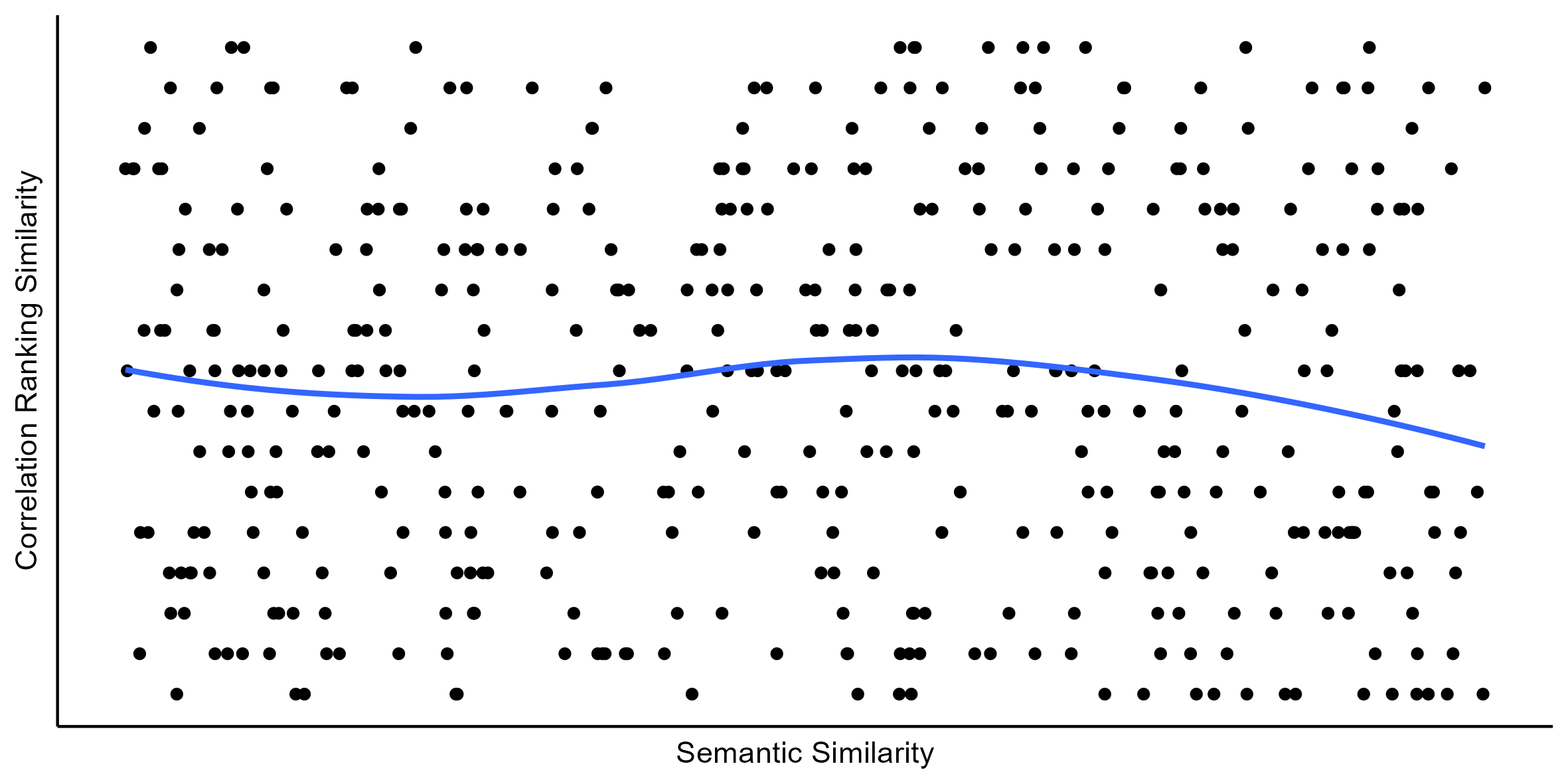
This plot would indicate poor vertical interpretability as there seems to be no relationship between semantic similarity and correlation ranking similarity. Now, consider Figure 3.

Figure 3: Sample Agreement Plot - Good Interpretability

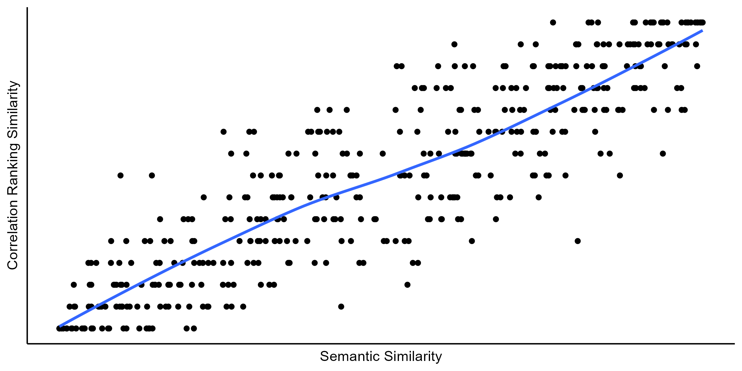
Here, there is good vertical interpretability since there appears to be a positive monotone relationship. That is, as the semantic similarity increases, the correlation ranking similarity or correlational similarity also increases. This would yield a high vertical interpretability index.

3.6 Horizontal Interpretability Index

This time, how distinct are the interpretations or meanings of the different factors from one another? Again, as mentioned in an earlier section, factors that have unique meanings make the model easier to interpret as the construct of interest can be broken down into distinct smaller constructs. For each factor $F_{k}$, define the central meaning of the factor as the embedding:

$$E_{k}=\frac{\sum_{i=1}^{M}{\left|\rho_{i,k}\right|\frac{G_{g}\left(Q_{i}\right)}{\left\lVert G_{g}\left(Q_{i}\right)\right\rVert}}}{\sum_{i=1}^{M}{\left|\rho_{i,k}\right|}}$$

Essentially, the factor $F_{k}$ is embedded in the same space as where the questions are embedded using $G_{g}$ as the weighted average of the normalized question embeddings, with the absolute correlations as the weights. The embeddings are normalized since the quantity of interest is the ”direction”. Note that since $G_{g}:Q\to\mathbb{R}^{Z}$, $E_{k}\in\mathbb{R}^{Z}$. Define $\bm{\underline{e}_{k}}$ as the vector from the origin to $E_{k}$, for each $E_{k}$. Then, intuitively, the factors have distinct meanings if $\bm{\underline{e}_{1}},\bm{\underline{e}_{2}},\dots,\bm{\underline{e}_{T}}$ are orthogonal. This is because the vector projection of one meaning on another meaning has a magnitude of 0, which can be interpreted as the non-overlap of meanings. Note that the angular distance between $\bm{\underline{e}_{i}}$ and $\bm{\underline{e}_{j}}$ is $\arccos{\frac{\bm{\underline{e}_{i}}\cdot\bm{\underline{e}_{j}}}{\left\lVert\bm{\underline{e}_{i}}\right\rVert\left\lVert\bm{\underline{e}_{j}}\right\rVert}}$. Then, a measure of how far away $\bm{\underline{e}_{i}}$ and $\bm{\underline{e}_{j}}$ are from being orthogonal is

$$\left|\arccos{\frac{\bm{\underline{e}_{i}}\cdot\bm{\underline{e}_{j}}}{\left\lVert\bm{\underline{e}_{i}}\right\rVert\left\lVert\bm{\underline{e}_{j}}\right\rVert}}-\frac{\pi}{2}\right|$$

For ease of interpretation, divide the measure by $\frac{\pi}{2}$ to get the distance

$$\frac{2}{\pi}\left|\arccos{\frac{\bm{\underline{e}_{i}}\cdot\bm{\underline{e}_{j}}}{\left\lVert\bm{\underline{e}_{i}}\right\rVert\left\lVert\bm{\underline{e}_{j}}\right\rVert}}-\frac{\pi}{2}\right|\in[0,1]$$

Thus, the average distance is simply

$$\frac{2}{T\left(T-1\right)}\sum_{i<j}{\frac{2}{\pi}\left|\arccos{\frac{\bm{\underline{e}_{i}}\cdot\bm{\underline{e}_{j}}}{\left\lVert\bm{\underline{e}_{i}}\right\rVert\left\lVert\bm{\underline{e}_{j}}\right\rVert}}-\frac{\pi}{2}\right|}$$

Hence, the horizontal interpretability index (or $H$-index) is:

$$B=1-\frac{4}{\pi T\left(T-1\right)}\sum_{i<j}{\left|\arccos{\frac{\bm{\underline{e}_{i}}\cdot\bm{\underline{e}_{j}}}{\left\lVert\bm{\underline{e}_{i}}\right\rVert\left\lVert\bm{\underline{e}_{j}}\right\rVert}}-\frac{\pi}{2}\right|}$$

Observe that $\bm{\underline{e}_{1}},\bm{\underline{e}_{2}},\dots,\bm{\underline{e}_{T}}$ are orthogonal (pairwise orthogonal) if and only if $H=1$. Ideally, larger values of $H$ indicate better horizontal interpretability. Note that this index also adds an assumption. The number of factors must be less than the dimensions of the embedding. That is, $T<Z$. This is because it is guaranteed that there exists at least one set of $n$ vectors in $\mathbb{R}^{Z}$ that are pairwise orthogonal when $n\leq Z$. However, this is not guaranteed when $n>Z$.

3.7 Overall Interpretability Index

Note that $V,H\in\left[0,1\right]$. Hence, if the point $\left(V,H\right)$ is plotted on the Cartesian plane, the region where the point can possibly be located is $\left\{\left(x,y\right):0\leq x,y\leq 1\right\}$, as shown by the square in Figure 4.

Figure 4: Set of possible points

Ideally, $\left(V,H\right)=\left(1,1\right)$. Moreover, ceteris paribus, higher values of $V$ are preferred. The same can be said for $H$. Thus, the distance of $\left(V,H\right)$ from $\left(1,1\right)$ can be interpreted as the deviation from the ideal condition, as shown in Figure 5.

Figure 5: Distance of $\left(V,H\right)$ from $\left(1,1\right)$

The distance is simply

$$\sqrt{\left(V-1\right)^{2}+\left(H-1\right)^{2}}$$

Note that $\sqrt{\left(V-1\right)^{2}+\left(H-1\right)^{2}}\in\left[0,\sqrt{2}\right]$. Thus, the overall interpretability index can be

$$I=1-\frac{\sqrt{2}}{2}\sqrt{\left(V-1\right)^{2}+\left(H-1\right)^{2}}$$

Note that the scaled distance is subtracted from 1 to facilitate easier interpretation. Furthermore, $I\in\left[0,1\right]$ and larger values of $I$ indicate better fit. Since points with the same distance from $\left(1,1\right)$ are deemed ”equally interpretable”, a kind of isoquant curves can also be drawn such that points that lie on the same curve are deemed as equally interpretable, as shown in Figure 6.

Figure 6: Isoquant curves for $\left(V,H\right)$

In Figure 6, suppose that points $P_{1},\dots,P_{4}$ correspond to factor models $\mathscr{F}_{1},\dots,\mathscr{F}_{4}$, respectively. Then, based on the overall interpretability index, $\mathscr{F}_{1}$ and $\mathscr{F}_{2}$ are equally interpretable. The same can be said for $\mathscr{F}_{3}$ and $\mathscr{F}_{4}$. However, $\mathscr{F}_{1}$ is more interpretable than $\mathscr{F}_{4}$ and so on. Assuming that all these models are equally statistically valid, then models $\mathscr{F}_{1}$ and $\mathscr{F}_{2}$ are preferred. Clearly, if $\left(V,H\right)=\left(x_{1},y_{1}\right)$ for model $\mathscr{F}_{A}$ and $\left(V,H\right)=\left(x_{2},y_{2}\right)$ for model $\mathscr{F}_{B}$, then $\mathscr{F}_{A}$ and $\mathscr{F}_{B}$ are equally interpretable if and only if

$$\left(x_{1}-1\right)^{2}+\left(y_{1}-1\right)^{2}=\left(x_{2}-1\right)^{2}+\left(y_{2}-1\right)^{2}$$

Basically, if the points lie on the same circle centered at $\left(1,1\right)$, they correspond to models that are equally interpretable. Assuming that both models are equally statistically valid, the model with the larger value for $I$ is preferred. Moreover, using the distance for $I$ is argued to be better than simply averaging $V,H\in\left[0,1\right]$ because this incorporates the concept of diminishing marginal rate of substitution. For example, if the value for $V$ is already low, then one would give up less of $V$ to increase $H$ since there will always be a point when $V$ just becomes ”too low” no matter how high $H$ is (and vice versa). Therefore, the overall interpretability index $I$ (or $I$-index) is given by

$$I=1-\frac{\sqrt{2}}{2}\sqrt{\left(V-1\right)^{2}+\left(H-1\right)^{2}},$$

where

$$V=\frac{1}{2}\left(\frac{N_{C}\left(Y\right)-N_{D}\left(Y\right)}{\sqrt{N\left(Y\right)-N_{1}\left(Y\right)}\sqrt{N\left(Y\right)-N_{2}\left(Y\right)}}+1\right)$$

$$H=1-\frac{4}{\pi T\left(T-1\right)}\sum_{\left(i<j\right)\wedge\left(i,j\in\left\{1,2,\dots,T\right\}\right)}{\left|\arccos{\frac{\bm{\underline{e}_{i}}\cdot\bm{\underline{e}_{j}}}{\left\lVert\bm{\underline{e}_{i}}\right\rVert\left\lVert\bm{\underline{e}_{j}}\right\rVert}}-\frac{\pi}{2}\right|}$$

It is important to note that $I$ is not necessarily a measure of absolute goodness-of-fit. It is much more useful as a measure of relative goodness-of-fit (that is, for comparing two or more factor models). With everything else equal, the model with the largest value for $I\in\left[0,1\right]$ is preferred. Ultimately, the entire procedure (i.e., the interpmax procedure) is as follows:

1. Calculate the semantic similarity for each pair of questions.

2. Fit different factor models and construct the set of candidate models $\mathscr{F}$. Members of $\mathscr{F}$ are considered equally statistically valid.

3. For each factor model, calculate the correlation ranking similarities for each pair of variables for each factor.

4. Calculate $V$ and $H$ for each factor model based on the semantic similarity matrix and the correlation ranking similarity matrices.

5. Calculate $I$ for each $F\in\mathscr{F}$.

6. Choose $F\in\mathscr{F}$ with the largest $I$.

Depending on the goals, only $V$ or only $H$ can be calculated instead of both and $I$.

Remark (Applicability to orthogonal and non-orthogonal factor models).

Note that index $V$ is applicable not just for orthogonal factor models, but also for oblique factor models. The premise and calculation of $V$ does not require orthogonality. However, $H$ is applicable only to orthogonal factor models since it is unreasonable to expect ”orthogonality of meanings” in non-orthogonal factor models. Thus, while $V$ is suitable for any factor model, both $H$ and $I$ should be used only for orthogonal models.

3.8 Extension to General Soft Constraints

Observe that the questions semantic similarity matrix $\bm{\underline{Q}}$ is essentially a priori information about the model. The indices measure how well the fitted factor models agrees with the prior information. In the case of the interpretability indices, the prior information is the semantics or the similarity of the meanings of the questions as quantified by the universal sentence encoder. Now, $\bm{\underline{Q}}$ does not actually have to be the semantic similarity of the questions calculated using the universal sentence encoder. Any other sentence encoder can be used to get the semantic similarity matrix. For example, a sentence encoder trained specifically on data related to the topic at hand could be used in order to provide a more accurate depiction of semantic similarity. Extending the interpmax procedure even further, the semantic similarity matrix does not even have to be about semantic similarity. It can be extended to a more general form called the soft constraints matrix or the prior matrix $\bm{\underline{C}}=\left(c_{i,j}\right)_{1\leq i,j\leq M}$ and the entire procedure can be extended to the priorimax procedure. The soft constraints matrix, then, provides a way to encode some prior information and eventually, measure the concordance of the fitted factor models with the prior information. For example, the investigator can construct the soft constraints matrix or prior matrix to reflect how the variables should, preferably, be grouped together based on existing theory or domain knowledge and then, use the vertical interpretability index to quantify how well the fitted models agree with the prior theory. In this case, the vertical interpretability index is more like an agreement index $A$. Then, the extended procedure would essentially be as follows:

1. Encode prior information into a soft constraints matrix $\bm{\underline{C}}$.

2. Fit different factor models and construct the set of candidate models $\mathscr{F}$. Members of $\mathscr{F}$ are considered equally statistically valid.

3. Calculate the agreement index $A$ for each $F\in\mathscr{F}$ based on $\bm{\underline{C}}$.

4. Choose the model $F\in\mathscr{F}$ with the agreement index $A$.

The interpmax procedure can be thought of as a special case of the priorimax procedure, where the soft constraints matrix is the semantic similarity matrix (and with the addition of the index $H$). Since the prior information is about semantics, the indices can be considered as interpretability indices. Particularly, $V$ is a special case of $A$. To give an example, suppose that there are five (5) variables - $X_{1},X_{2},\dots,X_{5}$. Then, suppose that based on existing domain knowledge, $X_{1}$ and $X_{2}$ are expected to be grouped together into one factor while $X_{3}$, $X_{4}$, and $X_{5}$ are expected to be grouped together into another. A possible soft constraints matrix $\bm{\underline{C}}$ would be

$$\begin{pmatrix}1&1&0&0&0\\ 1&1&0&0&0\\ 0&0&1&1&1\\ 0&0&1&1&1\\ 0&0&1&1&1\end{pmatrix}$$

If variables $X_{i}$ and $X_{j}$ are preferred to be grouped together over variables $X_{i}$ and $X_{k}$, then set $c_{i,j}>c_{i,k}$. If it is more important (or more preferred) to group $X_{i}$ and $X_{j}$ together than it is to group $X_{m}$ and $X_{n}$ together, then set $c_{i,j}>c_{m,n}$. The diagonal entries do not really matter. Also, because the agreement index $A$ uses the Kendall Tau-$b$ correlation, only the rankings of cells in $\bm{\underline{C}}$ are important, not the exact values. However, note that $\bm{\underline{C}}$ must be a symmetric matrix. More ”complex” relationships or information can be encoded in the soft constraints matrix. Essentially, $Y$ can be redefined as

$$Y=\left\{\left(c_{i,j},D_{f}\left(X_{i},X_{j}\right)\right):\left(i,j\in\left\{1,2,\dots,M\right\}\right)\wedge\left(i<j\right)\right\}$$

Observe that this definition is more ”general” because for each ordered pair, the value at the first index does not have to be (but can be) $D_{s}\left(G_{g}\left(Q_{i}\right),G_{g}\left(Q_{j}\right)\right)$. However, the previous example soft constraints matrix is not useful because if the investigators had that much detail about the possible structure (i.e., if there were a hypothesized complete partitioning of the observed variables), then they would probably be better off performing confirmatory factor analysis instead of exploratory factor analysis. A more realistic example would be

$$\begin{pmatrix}1&3&0&0&0\\ 3&1&0&0&0\\ 0&0&1&1&2\\ 0&0&1&1&2\\ 0&0&2&2&1\end{pmatrix}$$

One can also use something based on the semantic similarity matrix $\bm{\bm{\underline{Q}}}$, but not $\bm{\bm{\underline{Q}}}$ itself directly, as a soft constraints matrix. For instance, since $\bm{\bm{\underline{Q}}}$ is technically a similarity matrix, one can cluster the questions based on this similarity matrix. This can be done perhaps using affinity propagation, as in Frey & Dueck (2007a), or with $k$-medoids, as in Park & Jun (2009a). Then, the clustering of the questions based on semantic similarity can be written as a soft constraints matrix. In the next subsection, a partial matrix, which is also probably going to be more useful in application, is introduced. Now, the agreement index, then, measure how well a fitted factor model follows the ”groupings” defined in $\bm{\underline{C}}$. The investigator has to be careful that $\bm{\underline{C}}$ actually makes sense. The interpretability index (or more generally, the agreement index) operationalizes and extends the WOW criterion described by Johnson & Wichern (2007a). Moreover, even though it is assumed that the factor model is orthogonal, the indices (i.e., $V$, $H$, $I$, and $A$) and procedures (i.e., the interpmax and priorimax procedures) are actually still applicable to non-orthogonal factor models (although, there is special consideration for $H$ as remarked earlier). However, it is emphasized that the indices are most useful as measures of relative goodness-of-fit (i.e., for comparisons).

3.9 Partial Soft Constraints Matrix

Normally, the soft constraints matrix should have values for each of its $M\times M$ cells. However, there may be cases when not all pairs have prior information. Fortunately, the agreement index can be modified to accommodate soft constraints matrices with incomplete entries, which are called partial soft constraints matrices. Let $\Delta$ denote a null value (i.e., no value or no prior information). Then, the definition of the multiset $Y$ can be modified as follows:

$$Y=\left\{\left(c_{i,j},D_{f}\left(X_{i},X_{j}\right)\right):\left(i,j\in\left\{1,2,\dots,M\right\}\right)\wedge\left(i<j\right)\wedge\left(c_{i,j}\neq\Delta\right)\right\}$$

Essentially, pairs of variables with no prior information (i.e., pairs $\left(X_{i},X_{j}\right)$ such that $c_{i,j}=\Delta$) are simply excluded from the calculation of the agreement index. The agreement index $A$ remains to be the Kendall Tau-$b$ correlation coefficient based on $Y$ as redefined above. For example, suppose again that there are five (6) variables $X_{1},\dots,X_{6}$. Next, suppose that $X_{1}$ and $X_{3}$ should be grouped together and $X_{4}$ and $X_{6}$ should be grouped together. However, it is unknown how $X_{2}$ and $X_{5}$ should be grouped (i.e., there is no prior information about these two variables). Then, a possible partial soft constraints matrix $\bm{\underline{C}}$ would be

$$\begin{pmatrix}1&\Delta&1&0&\Delta&0\\ \Delta&\Delta&\Delta&\Delta&\Delta&\Delta\\ 1&\Delta&1&0&\Delta&0\\ 0&\Delta&0&1&\Delta&1\\ \Delta&\Delta&\Delta&\Delta&\Delta&\Delta\\ 0&\Delta&0&1&\Delta&1\end{pmatrix}$$

The agreement index $A$ still provides a measure of concordance with the prior information or expectation represented in $\bm{\underline{C}}$ as it still acts on the available information in a way similar to how it does for a fully specified $\bm{\underline{C}}$. Although this time, it is invariant with respect to models whose only differences are in variable relationships with no prior information (i.e., relationships whose prior information is $\Delta$).

3.10 The Priorimax and Interpmax Rotations

As discussed in the previous sections, the vertical interpretability index $V$ (or more generally, the agreement index $A$) can be considered as an interpretability index and so, is a goodness-of-fit criterion. Then, a rotation method can be built on $A$. What factor rotation maximizes $A$? This can be solved as an optimization problem. Recall that

$$A=\frac{1}{2}\left(\frac{N_{C}\left(Y\right)-N_{D}\left(Y\right)}{\sqrt{N\left(Y\right)-N_{1}\left(Y\right)}\sqrt{N\left(Y\right)-N_{2}\left(Y\right)}}+1\right)$$

Note that the agreement index can be expressed as a function of the orthogonal rotation matrix $\bm{\underline{R}}$ (which is square with dimensions $T\times T$) when the unrotated loadings $\bm{\underline{L}}$, the components $\bm{\underline{X}}$, and the soft constraints (i.e., prior information) $\bm{\underline{C}}$ are known:

$$A=f\left(\bm{\underline{R}};\bm{\underline{L}},\bm{\underline{X}},\bm{\underline{C}}\right)$$

We can then find an orthogonal rotation matrix $\bm{\underline{R}}$ that generates the new loading matrix $\bm{\underline{L}}^{*}=\bm{\underline{L}}\bm{\underline{R}}$ such that $\max{A}=f\left(\bm{\underline{R}};\bm{\underline{L}},\bm{\underline{X}},\bm{\underline{C}}\right)$. Thus, the priorimax rotation (or the process of finding) $\bm{\underline{R}}$ is the optimization problem

$$\underset{\displaystyle\bm{\underline{R}}}{\mathrm{max}}\hskip 9.24994ptA$$

$$\mathmakebox[\widthof{$\underset{\displaystyle\phantom{\bm{\underline{R}}}}{\mathrm{max}}$}][c]{\mathmakebox[\widthof{$\mathrm{max}$}][l]{\mathrm{\kern 0.92505pts.t.}}}\hskip 9.24994pt \bm{\underline{R}}\bm{\underline{R}}^{\prime}=\bm{\underline{I}}$$

However, the constraint is $\bm{\underline{R}}\bm{\underline{R}}^{\prime}=\bm{\underline{I}}$ is numerically unstable and may not be the most efficient way to express the orthogonality constraint. For instance, the decision variables are unbounded in this parametrization. To solve this, we can reparametrize $\bm{\underline{R}}$ using the Cayley transformation $h$ of a matrix $\bm{\underline{M}}$, given by $h\left(\bm{\underline{M}}\right)=\left(\bm{\underline{I}}-\bm{\underline{M}}\right)\left(\bm{\underline{I}}+\bm{\underline{M}}\right)^{-1}$. From the fact that the Cayley transformation is an involution and from the works of Kahan (2006a) and O’Dorney (2014a), it is easy to see that for any real square orthogonal matrix $\bm{\underline{R}}$, there exists a skew-symmetric matrix $\bm{\underline{S}}$ with all entries in $\left[-1,1\right]$ and a signature matrix $\bm{\underline{D}}$ (i.e., a diagonal matrix with diagonal entries $\pm 1$) such that

$$\bm{\underline{R}}=\left(\bm{\underline{I}}-\bm{\underline{S}}\right)\left(\bm{\underline{I}}+\bm{\underline{S}}\right)^{-1}\bm{\underline{D}}$$

Moreover, for any skew-symmetric matrix $\bm{\underline{S}}$ and any signature matrix $\bm{\underline{D}}$, $\left(\bm{\underline{I}}-\bm{\underline{S}}\right)\left(\bm{\underline{I}}+\bm{\underline{S}}\right)^{-1}\bm{\underline{D}}$ is always orthogonal. Now, let $\bm{\underline{S}}=\left(s_{i,j}\right)_{1\leq i,j\leq T}$ and $\bm{\underline{D}}=\text{diag}\left(d_{1},\dots,d_{T}\right)$, where $s_{i,j}=-s_{j,i}$ for all $i<j$. Using the Cayley-style representation, the optimization problem can then be re-written as

$$\underset{\displaystyle\bm{\underline{S}},\bm{\underline{D}}}{\mathrm{max}}\hskip 9.24994ptA=g\left(\bm{\underline{S}},\bm{\underline{D}};\bm{\underline{L}},\bm{\underline{X}},\bm{\underline{C}}\right)$$

$$\mathmakebox[\widthof{$\underset{\displaystyle\phantom{\bm{\underline{S}},\bm{\underline{D}}}}{\mathrm{max}}$}][c]{\mathmakebox[\widthof{$\mathrm{max}$}][l]{\mathrm{\kern 0.92505pts.t.}}}\hskip 9.24994pt \left(\forall i\right)\left(d_{i}^{2}-1=0\right),$$

$$\left(\forall i<j\right)\left(-1\leq s_{i,j}\leq 1\right)$$

The $\frac{T^{2}+T}{2}$ decision parameters are $s_{1,2},s_{1,3},\dots,s_{1,T},s_{2,3},\dots,s_{2,T},\dots,s_{T-1,T},d_{1},d_{2},\dots,d_{T}$. There are $T$ nonlinear equality constraints, $\frac{T^{2}-T}{2}$ box constraints, and $1$ objective function. Note that the rotation matrix $\bm{\underline{R}}$ can be completely obtained from $\bm{\underline{S}}$ and $\bm{\underline{D}}$. This can be solved using the Improved Stochastic Ranking Evaluation Strategy (ISRES) optimization algorithm, which was developed by Runarsson & Yao (2005a) and is implemented in the NLopt library by Johnson (2007a). The ISRES algorithm is used since it is a gradient-free global optimization algorithm that supports nonlinear equality constraints. The same optimization problem except with the objective function being $I$ instead of $A$ yields the interpmax rotation. An implementation of the rotation methods (or optimization problems) is demonstrated in the next section using a Python package we created called interpretablefa.

3.11 On the Factor Score Indeterminacy Problem

The proposed procedures and indices here do not face the factor score indeterminacy problem as the estimation of factor scores is not required. To show this, rewrite the model as

$$\bm{\underline{X}}=\bm{\underline{\mu}}+\bm{\underline{L}}\bm{\underline{F}}+\bm{\underline{\varepsilon}},$$

where $\bm{\underline{X}}$ are the observed variables with mean $\bm{\underline{\mu}}$, $\bm{\underline{L}}$ is the factor loading matrix, $\bm{\underline{F}}$ are the unobservable common factors, and $\bm{\underline{\varepsilon}}$ are the error terms. As shown in Johnson & Wichern (2007a),

$$\text{Cov}\left(\bm{\underline{X}},\bm{\underline{F}}\right)=\mathbb{E}\left(\bm{\underline{X}}-\bm{\underline{\mu}}\right)\bm{\underline{F}}^{\prime}=\bm{\underline{L}}\mathbb{E}\left(\bm{\underline{F}}\bm{\underline{F}}^{\prime}\right)+\mathbb{E}\left(\bm{\underline{\varepsilon}}\bm{\underline{F}}^{\prime}\right)=\bm{\underline{L}}$$

Now, note that

$$\rho_{i,j}=\corr\left(X_{i},F_{j}\right)=\frac{\text{Cov}\left(X_{i},F_{j}\right)}{\sqrt{\text{Var}\left(X_{i}\right)\text{Var}\left(F_{j}\right)}}$$

However, for orthogonal factor models, $\text{Cov}\left(\bm{\underline{F}}\right)=\bm{\underline{I}}$ and so, $\text{Var}\left(F_{j}\right)=1$ (note that $\text{Var}\left(F_{j}\right)=1$ is also true for oblique factor models). Thus,

$$\corr\left(X_{i},F_{j}\right)=\frac{l_{i,j}}{\sqrt{\text{Var}\left(X_{i}\right)}},$$

, where $l_{i,j}$ is the loading of $X_{i}$ on $F_{j}$. Then,

$$S_{i,j}=\left\{\left(\left|\rho_{i,k}\right|,\left|\rho_{j,k}\right|\right):k\in\left\{1,2,\dots,T\right\}\right\}=\left\{\left(\left|\frac{l_{i,k}}{\sqrt{\text{Var}\left(X_{i}\right)}}\right|,\left|\frac{l_{j,k}}{\sqrt{\text{Var}\left(X_{j}\right)}}\right|\right):k\in\left\{1,2,\dots,T\right\}\right\},$$

which means that generating the set $S_{i,j}$ does not require the estimation of factor scores. Consequently, $D_{f}\left(X_{i},X_{j}\right)$ does not require the estimation of factor scores. Moreover, the soft constraints matrix $\bm{\underline{C}}$ is specified even before factor analysis is done so it also does not require the estimation of factor scores. Consequently, $V$, $A$, $H$, and $I$ are calculated independent of the factor scores. Note that a similar argument can be made for oblique factor models since the calculation of $D_{f}$ is still just based on $\bm{\underline{L}}$, the variances of $\bm{\underline{X}}$, and, this time, the rotation matrix. Therefore, for any factor model, the procedures and indices do not require the estimation of factor scores - avoiding the factor indeterminacy problem.

3.12 Remarks

3.12.1 Relaxing Assumptions

Recall from earlier that one assumption was that a realization for each $X_{k}$ is a response from a $p$-point Likert (or Likert-type) item and is integer-valued with range $W=\left\{1,2,\dots,p\right\}$. That is, for each $X_{k}$, $n$ realized values are obtained, one each from the respondents $\left(r_{1}\right)_{g},\left(r_{2}\right)_{g},\dots,\left(r_{n}\right)_{g}$, where

$$\left(r_{j}\right)_{g}=D_{j}\left(G_{g}\left(Q_{k}\right)\right)+\delta_{j,k}$$

This assumption is important for the interpmax procedure (or whenever the soft constraints matrix is based on semantic similarity, using the universal sentence encoder or any other kind of embedding). This is because the use of semantic similarity involves using the questions or sentences. However, this assumption can be relaxed whenever the soft constraints matrix is not about semantic similarity. For example, if the soft constraints matrix is based on some other domain knowledge instead of the semantic similarities, the responses do not have to be from Likert or Likert-type items and the responses do not have to be conceptualized as functions of the sentences (i.e., questions). This is because the soft constraints matrix is simply an encoding of prior information and does not necessarily have to be dependent on the meanings of the questions. For example, it can be used when the observations are not taken from humans.

3.12.2 On Choosing an Embedding

Note that when using semantic similarities for the soft constraints or prior matrix, it is important to choose an embedding model that is appropriate for the context of the study. Here, by default, the universal sentence encoder is used. However, depending on the specific research topic, there may be an embedding model that is more appropriate (e.g., using a model whose training data consist mostly of items directly related to the topics at hand). It is also important to be aware of the limitations of the embedding function or model. For instance, the embedding model might consider a statement and its negation as almost completely semantically similar even though they are contextually opposite (e.g., using the word ”not”). The embedding and the questions must be aligned on matters like this.

4 Implementation and Example

4.1 Software Implementation

For the software implementation of the proposed indices, procedures, rotations, and visualizations, we created a Python class called InterpretableFA, bundled as the interpretablefa package. The InterpretableFA class also includes helper methods, including several visualizations and another to generate prior matrices. It also provides several wrapper functions for some methods in the FactorAnalyzer class from the Python package factor_analyzer. The package interpretablefa is made available on the Python Package Index. Its official documentation is also made accessible there. Lastly, the proposed methods and the interpretablefa package (e.g., rotations, indices, visualizations, etc.) are demonstrated in the next parts.

4.2 Empirical Example

4.2.1 Indices and Procedures

The demonstration uses the Experiences in Close Relationships Scale (ECR), developed by Kelly Brennan, Catherine Clark and Phillip Shaver in 1998. It was originally designed to test the attachment style of an individual, or see how they behave in their romantic relationships with other people. The ECR consists of 36 statements answered on a 5-point Likert scale. Higher scores indicate greater agreement with the item (1 = strongly disagree, 2 = disagree, 3 = neutral, 4 = agree, and 5 = strongly agree). Raw dataset for this scale was obtained from the Open-Source Psychometrics Project (2019a), a publicly-available online platform for psychological research, acquiring a total of 49,934 sample points. Before conducting Exploratory Factor Analysis (EFA), data adequacy was assessed using the calculate_indices function. Bartlett’s Test of Sphericity indicated significant correlations among the ECR variables ($p<0.05$). The overall Measure of Sampling Adequacy (MSA) was 0.95, with individual MSA values classified as ’marvelous’ according to Kaiser’s Rule, suggesting excellent sampling adequacy. Consequently, no variables were excluded. For this demonstration, orthogonal rotations were employed, emphasizing semantic similarity. In EFA, we prioritize the interpretability of grouped variables while identifying candidate factor models that best fit the data and are most interpretable. For this example, we select four models: the equamax 4-factor model, the oblimax 4-factor model, the varimax 3-factor model, and the quartimax 3-factor model. The variable-factor correlations resulting from these rotation models are depicted in the heatmaps below.

Figure 7: Variable-Factor Correlation of Equamax 4-factor Rotation Model

Figure 8: Variable-Factor Correlation of Oblimax 4-factor Rotation Model

Figure 9: Variable-Factor Correlation of Varimax 3-factor Rotation Model

Figure 10: Variable-Factor Correlation of Quartimax 3-factor Rotation Model

To identify the factor model with the best interpretability, we will employ two recently introduced methods: interpmax and priorimax. We have already calculated the semantic similarities between question pairs and the correlation ranking similarities between variables for each extracted factor. Next, we need to compute the vertical, horizontal, and overall indices for each candidate model. For this comparison, it is important to assume that all models are equally statistically valid. The results of these calculations, using the calculate_indices function, are presented in the table below. Table 1. Indices of Candidate Models Model Vertical Index Horizontal Index Overall Index 4-Factor Model Equamax Rotation 0.5439 0.2288 0.3665 4-Factor Model Oblimax Rotation 0.5856 0.1841 0.3529 3-Factor Model Varimax Rotation 0.5546 0.2394 0.3768 3-Factor Model Quartimax Rotation 0.5345 0.2232 0.3596 We can also examine the scatterplot of the agreement indices for each model using the visualize_interpretability function, which includes a LOWESS curve. For example, we might want to view the agreement plot for the 3-factor varimax rotation model and the 3-factor quartimax rotation model.

Figure 11: Agreement Plot for Varimax 3-factor Model

Figure 12: Agreement Plot for Quartimax 3-factor Model

Two procedures are presented in this paper for selecting the most interpretable model. In the interpmax procedure, we choose the factor model with the highest overall index (or $I$-index), which is the 3-factor model from the varimax rotation. On the other hand, in the priorimax procedure, we select the factor model with the highest agreement (also called as vertical in this case) index (or $A$-index), which is the 4-factor model from the oblimax rotation. For this example, we will follow the interpmax procedure, given that we are using semantic similarities as the soft constraints. Accordingly, we select the factor model with the highest overall index, which is the 3-factor model from the varimax rotation. To visualize the vertical index, horizontal index, overall index, and isoquant curve, we can use the visualize_interpretability function.

Figure 13: Isoquant Curve for Indices of Candidate Models

4.2.2 Rotating Based on a Soft Constraints Matrix

To demonstrate the Priorimax rotation (an orthogonal rotation) with a soft constraints matrix (i.e., a partition of a subset of questions or observable variables), a 4-factor model is fit with the priorimax rotation based on a soft constraints matrix $\bm{\underline{C}}=\left(c_{i,j}\right)_{1\leq i,j\leq 36}$. Define the following sets:

$$P_{1}=\left\{1,7,9,11,13,17,23\right\},P_{2}=\left\{6,10,12\right\},P_{3}=\left\{14,16,26,36\right\},P_{4}=\left\{20,28,32,34\right\}$$

Furthermore, let $P=\bigcup_{i}{P_{i}}$. Observe that $P_{i}\cap P_{j}=\varnothing$ for all $i\neq j$. Then, suppose that the soft constraints matrix $\bm{\underline{C}}$ is given by

$$c_{i,j}=\begin{cases}1,&\text{if }\left(\exists k\right)\left(i,j\in P_{k}\right)\\ 0,&\text{if }\left(\left(\forall k\right)\left(i,j\notin P_{k}\right)\right)\wedge\left(i,j\in P\right)\\ \Delta,&\text{if }\left(i\notin P\right)\vee\left(j\notin P\right)\end{cases}$$

This means that $\left\{X_{1},X_{7},X_{9},X_{11},X_{13},X_{17},X_{23}\right\}$ are grouped together, $\left\{X_{6},X_{10},X_{12}\right\}$ are grouped together, $\left\{X_{14},X_{16},X_{26},X_{36}\right\}$ are grouped together, and $\left\{X_{20},X_{28},X_{32},X_{34}\right\}$ are grouped together all through $\bm{\underline{C}}$. Meanwhile, there is no prior information in $\bm{\underline{C}}$ for all $X_{i}$ such that $i\notin P$. Using the newly developed Python package, interpretablefa, to fit the model:

The best rotation matrix (i.e., the priorimax rotation) is given by





$$\bm{\underline{R}}\approx\begin{pmatrix}0.0039&0.4013&-0.2748&-0.8737\\
-0.1970&-0.0587&-0.9412&0.2682\\
-0.6483&-0.6768&0.0812&-0.3393\\
-0.7355&0.6144&0.1791&0.2226\end{pmatrix}$$

The estimated model’s $A$-index is about $0.8123$. The visualizations can also be generated for this model using the interpretablefa package. For example, the agreement plot for this model is shown below.


Figure 14: Agreement Plot for Priorimax 4-factor Model



5 Conclusion and Recommendations


In this paper, a new method of measuring the interpretability of a factor model is presented. In this method, a way of encoding prior information (such as semantic similarity) and measuring the model’s concordance with such is developed. Moreover, in connection with these, simple model selection procedures and rotation methods using mathematical optimization are proposed.
The methods provide several advantages. First, it allows for a very flexible specification of the prior information or expected relationships, allowing for partial and/or complete pairwise specifications of relationships. Second, it provides a way to directly take into account the role of language and semantics when it comes to responses from humans. Third, the method does not require the estimation of factor scores, which avoids the factor score indeterminacy problems.
With that being said, there are several extensions that can be done for the method. One is to develop a more comprehensive index based on the interpretability indices in the method. The proposed indices are mostly based on ”agreement” but does not take into account the goodness-of-fit in terms of variances. A composite index based on this ”agreement” and a variance-based goodness-of-fit index could be useful. Another is to come up with a better way of calculating the rotation (i.e., a better way of maximizing $A$, $V$, or $I$). The mathematical program and optimization method outlined here may not be the most computationally efficient or accurate.
Exploring other similarity measures, still based on correlations or loadings, for the observable variables or components may also be useful. For instance, one could define a within-factor index for a given factor $F_{k}$ that that defines correlation similarity as




$$1-\left|\left|\rho_{i,k}\right|-\left|\rho_{j,k}\right|\right|,$$


where $\rho_{i,k}$ and $\rho_{j,k}$ are the correlations of $X_{i}$ and of $X_{j}$ with $F_{k}$, respectively. Then, such within-factor indices could be summarized into a single measure (perhaps by taking the arithmetic mean or the minimum). Another example is to use the Pearson correlation, as defined in Bluman (2012a), instead of the Kendall Tau-$b$ to impose a stricter condition (i.e., linearity and not just monotonicity).
Ultimately, the proposed indices showcase a novel way of measuring and achieving interpretability, as well as procedures and factor rotations based on them. Moreover, this paper can serve as foundation for exploring the idea of directly incorporating semantics and natural language processing techniques in factor models further.


Acknowledgements


The authors would like to thank Noeliano Ocorro and Rienyl Aiken Bacongallo for participating in brainstorming sessions during the early stages of the research study.

References

- Abdi (2003) Hervé Abdi “Factor Rotations in Factor Analyses”, 2003 URL: https://api.semanticscholar.org/CorpusID:14726876
- Abraham et al. (2021) Olufunmilola Abraham et al. “Development of the Adolescent Opioid Safety and Learning (AOSL) scale using exploratory factor analysis” In Res Social Adm Pharm 18.5, 2021, pp. 2796–2803
- Bluman (2012) Allan. Bluman “Elementary Statistics: A Step by Step Approach” McGraw-Hill Education, 2012
- Carrizosa et al. (2020) Emilio Carrizosa, Vanesa Guerrero, Dolores Morales and Albert Satorra “Enhancing Interpretability in Factor Analysis by Means of Mathematical Optimization” PMID: 31663785 In Multivariate Behavioral Research 55.5 Routledge, 2020, pp. 748–762 DOI: 10.1080/00273171.2019.1677208
- Cer et al. (2018) Daniel Cer et al. “Universal Sentence Encoder” In submission In In submission to: EMNLP demonstration, 2018 URL: https://arxiv.org/abs/1803.11175
- Cleveland (1979) William. Cleveland “Robust Locally Weighted Regression and Smoothing Scatterplots” In Journal of the American Statistical Association 74.368 ASA Website, 1979, pp. 829–836 DOI: 10.1080/01621459.1979.10481038
- Fan et al. (2016) Jianqing Fan, Yuan Liao and Weichen Wang “Projected principal component analysis in factor models” In The Annals of Statistics 44.1 Institute of Mathematical Statistics, 2016, pp. 219–254 DOI: 10.1214/15-AOS1364
- Floyd & Widaman (1995) Frank Floyd and Keith Widaman “Factor Analysis in the Development and Refinement of Clinical Assessment Instruments” In Psychological Assessment 7, 1995, pp. 286–299 DOI: 10.1037/1040-3590.7.3.286
- Frey & Dueck (2007) Brendan Frey and Delbert Dueck “Clustering by passing messages between data points” In Science 315.5814, 2007, pp. 972–976
- Geweke & Singleton (1980) John. Geweke and Kenneth. Singleton “Interpreting the Likelihood Ratio Statistic in Factor Models when Sample Size is Small” In Journal of the American Statistical Association 75.369 [American Statistical Association, Taylor & Francis, Ltd.], 1980, pp. 133–137 URL: http://www.jstor.org/stable/2287400
- Gorusch (1983) Richard. Gorusch “Factor Analysis” Psychology Press, 1983 DOI: https://doi.org/10.4324/9780203781098
- Harerimana & Mtshali (2020) Alexis Harerimana and Ntombifikile Mtshali “Using Exploratory and Confirmatory Factor Analysis to understand the role of technology in nursing education” In Nurse Education Today 92, 2020, pp. 104490 DOI: https://doi.org/10.1016/j.nedt.2020.104490
- Harpe (2015) Spencer. Harpe “How to analyze Likert and other rating scale data” In Currents in Pharmacy Teaching and Learning 7.6, 2015, pp. 836–850 DOI: https://doi.org/10.1016/j.cptl.2015.08.001
- Johnson & Wichern (2007) Richard. Johnson and Dean. Wichern “Applied Multivariate Statistical Analysis” Pearson, 2007, pp. 808
- Johnson (2007) Steven. Johnson “The NLopt nonlinear-optimization package”, https://github.com/stevengj/nlopt, 2007
- Kahan (2006) W. Kahan “Is there a small skew Cayley transform with zero diagonal?” Special Issue in honor of Friedrich Ludwig Bauer In Linear Algebra and its Applications 417.2, 2006, pp. 335–341 DOI: https://doi.org/10.1016/j.laa.2005.08.027
- Lara et al. (1992) B.. Lara, E. Tartas and P. Oyarzabal “Semantics and factor analysis: An approach to the interpretation of factors” In Applied Stochastic Models and Data Analysis 8.1, 1992, pp. 7–16 DOI: https://doi.org/10.1002/asm.3150080103
- Laurett et al. (2021) Rozélia Laurett, Arminda Paço and Emerson Mainardes “Measuring sustainable development, its antecedents, barriers and consequences in agriculture: An exploratory factor analysis” In Environmental Development 37, 2021, pp. 100583 DOI: https://doi.org/10.1016/j.envdev.2020.100583
- Ledesma et al. (2021) Rubén. Ledesma et al. “Exploratory factor analysis in transportation research: Current practices and recommendations” In Transportation Research Part F: Traffic Psychology and Behaviour 78, 2021, pp. 340–352 DOI: https://doi.org/10.1016/j.trf.2021.02.021
- Li & Jung (2017) Gen Li and Sungkyu Jung “Incorporating Covariates Into Integrated Factor Analysis of Multi-View Data” In Biometrics 73.4, 2017, pp. 1433–1442 DOI: 10.1111/biom.12698
- O’Dorney (2014) Evan O’Dorney “Minimizing the Cayley transform of an orthogonal matrix by multiplying by signature matrices” In Linear Algebra and its Applications 448, 2014, pp. 97–103 DOI: https://doi.org/10.1016/j.laa.2014.01.032
- Open-Source Psychometrics Project (2019) Open-Source Psychometrics Project “Open-Source Psychometrics Project” Accessed on June 25, 2024, 2019 URL: https://openpsychometrics.org/_rawdata/
- Park & Jun (2009) Hae-Sang Park and Chi-Hyuck Jun “A simple and fast algorithm for K-medoids clustering” In Expert Systems with Applications 36.2, Part 2, 2009, pp. 3336–3341 DOI: https://doi.org/10.1016/j.eswa.2008.01.039
- Pervin et al. (2005) L.A. Pervin, D. Cervone and O.P. John “Personality: Theory and Research” Wiley, 2005 URL: https://books.google.com.ph/books?id=_yIRAQAAIAAJ
- Runarsson & Yao (2005) T.P. Runarsson and Xin Yao “Search biases in constrained evolutionary optimization” In IEEE Transactions on Systems, Man, and Cybernetics, Part C (Applications and Reviews) 35.2, 2005, pp. 233–243 DOI: 10.1109/TSMCC.2004.841906
- Sass & Schmitt (2010) Daniel. Sass and Thomas. Schmitt “A Comparative Investigation of Rotation Criteria Within Exploratory Factor Analysis” PMID: 26789085 In Multivariate Behavioral Research 45.1 Routledge, 2010, pp. 73–103 DOI: 10.1080/00273170903504810
- Shrestha (2021) Noora Shrestha “Factor Analysis as a Tool for Survey Analysis” In American Journal of Applied Mathematics and Statistics 9, 2021, pp. 4–11 DOI: 10.12691/ajams-9-1-2
- Siegel (1956) Sidney Siegel “Nonparametric statistics for the behavioral sciences” McGraw-Hill, 1956
- Taeb et al. (2017) A. Taeb, J.. Reager, M. Turmon and V. Chandrasekaran “A Statistical Graphical Model of the California Reservoir System” In Water Resources Research 53.11, 2017, pp. 9721–9739 DOI: https://doi.org/10.1002/2017WR020412
- Taeb & Chandrasekaran (2018) Armeen Taeb and Venkat Chandrasekaran “Interpreting latent variables in factor models via convex optimization” In Mathematical Programming 167.1, 2018, pp. 129–154 DOI: 10.1007/s10107-017-1187-7
- Trninić et al. (2013) Viktorija Trninić, Igor Jelaska and Janez Stalec “Appropriateness and limitations of factor analysis methods utilized in psychology and kinesiology: Part II” In Fizicka kultura 67, 2013, pp. 5–17 DOI: 10.5937/fizkul1202077T
- William Revelle (2024) William Revelle “psych: Procedures for Psychological, Psychometric, and Personality Research” R package version 2.4.3, 2024 Northwestern University URL: https://CRAN.R-project.org/package=psych
- Williams et al. (2010) Brett Williams, Ted Brown and Andrys Onsman “Exploratory Factor Analysis: A Five-Step Guide for Novices” In Australasian Journal of Paramedicine 8, 2010, pp. 1–13 DOI: 10.33151/ajp.8.3.93
- Yamamoto et al. (2017) Michio Yamamoto, Kei Hirose and Haruhisa Nagata “Graphical tool of sparse factor analysis” In Behaviormetrika 44.1, 2017, pp. 229–250 DOI: 10.1007/s41237-016-0007-3
- Abdi (2003a) Hervé Abdi “Factor Rotations in Factor Analyses”, 2003 URL: https://api.semanticscholar.org/CorpusID:14726876
- Abraham et al. (2021a) Olufunmilola Abraham et al. “Development of the Adolescent Opioid Safety and Learning (AOSL) scale using exploratory factor analysis” In Res Social Adm Pharm 18.5, 2021, pp. 2796–2803
- Bluman (2012a) Allan. Bluman “Elementary Statistics: A Step by Step Approach” McGraw-Hill Education, 2012
- Carrizosa et al. (2020a) Emilio Carrizosa, Vanesa Guerrero, Dolores Morales and Albert Satorra “Enhancing Interpretability in Factor Analysis by Means of Mathematical Optimization” PMID: 31663785 In Multivariate Behavioral Research 55.5 Routledge, 2020, pp. 748–762 DOI: 10.1080/00273171.2019.1677208
- Cer et al. (2018a) Daniel Cer et al. “Universal Sentence Encoder” In submission In In submission to: EMNLP demonstration, 2018 URL: https://arxiv.org/abs/1803.11175
- Cleveland (1979a) William. Cleveland “Robust Locally Weighted Regression and Smoothing Scatterplots” In Journal of the American Statistical Association 74.368 ASA Website, 1979, pp. 829–836 DOI: 10.1080/01621459.1979.10481038
- Fan et al. (2016a) Jianqing Fan, Yuan Liao and Weichen Wang “Projected principal component analysis in factor models” In The Annals of Statistics 44.1 Institute of Mathematical Statistics, 2016, pp. 219–254 DOI: 10.1214/15-AOS1364
- Floyd & Widaman (1995a) Frank Floyd and Keith Widaman “Factor Analysis in the Development and Refinement of Clinical Assessment Instruments” In Psychological Assessment 7, 1995, pp. 286–299 DOI: 10.1037/1040-3590.7.3.286
- Frey & Dueck (2007a) Brendan Frey and Delbert Dueck “Clustering by passing messages between data points” In Science 315.5814, 2007, pp. 972–976
- Geweke & Singleton (1980a) John. Geweke and Kenneth. Singleton “Interpreting the Likelihood Ratio Statistic in Factor Models when Sample Size is Small” In Journal of the American Statistical Association 75.369 [American Statistical Association, Taylor & Francis, Ltd.], 1980, pp. 133–137 URL: http://www.jstor.org/stable/2287400
- Gorusch (1983a) Richard. Gorusch “Factor Analysis” Psychology Press, 1983 DOI: https://doi.org/10.4324/9780203781098
- Harerimana & Mtshali (2020a) Alexis Harerimana and Ntombifikile Mtshali “Using Exploratory and Confirmatory Factor Analysis to understand the role of technology in nursing education” In Nurse Education Today 92, 2020, pp. 104490 DOI: https://doi.org/10.1016/j.nedt.2020.104490
- Harpe (2015a) Spencer. Harpe “How to analyze Likert and other rating scale data” In Currents in Pharmacy Teaching and Learning 7.6, 2015, pp. 836–850 DOI: https://doi.org/10.1016/j.cptl.2015.08.001
- Johnson & Wichern (2007a) Richard. Johnson and Dean. Wichern “Applied Multivariate Statistical Analysis” Pearson, 2007, pp. 808
- Johnson (2007a) Steven. Johnson “The NLopt nonlinear-optimization package”, https://github.com/stevengj/nlopt, 2007
- Kahan (2006a) W. Kahan “Is there a small skew Cayley transform with zero diagonal?” Special Issue in honor of Friedrich Ludwig Bauer In Linear Algebra and its Applications 417.2, 2006, pp. 335–341 DOI: https://doi.org/10.1016/j.laa.2005.08.027
- Lara et al. (1992a) B.. Lara, E. Tartas and P. Oyarzabal “Semantics and factor analysis: An approach to the interpretation of factors” In Applied Stochastic Models and Data Analysis 8.1, 1992, pp. 7–16 DOI: https://doi.org/10.1002/asm.3150080103
- Laurett et al. (2021a) Rozélia Laurett, Arminda Paço and Emerson Mainardes “Measuring sustainable development, its antecedents, barriers and consequences in agriculture: An exploratory factor analysis” In Environmental Development 37, 2021, pp. 100583 DOI: https://doi.org/10.1016/j.envdev.2020.100583
- Ledesma et al. (2021a) Rubén. Ledesma et al. “Exploratory factor analysis in transportation research: Current practices and recommendations” In Transportation Research Part F: Traffic Psychology and Behaviour 78, 2021, pp. 340–352 DOI: https://doi.org/10.1016/j.trf.2021.02.021
- Li & Jung (2017a) Gen Li and Sungkyu Jung “Incorporating Covariates Into Integrated Factor Analysis of Multi-View Data” In Biometrics 73.4, 2017, pp. 1433–1442 DOI: 10.1111/biom.12698
- O’Dorney (2014a) Evan O’Dorney “Minimizing the Cayley transform of an orthogonal matrix by multiplying by signature matrices” In Linear Algebra and its Applications 448, 2014, pp. 97–103 DOI: https://doi.org/10.1016/j.laa.2014.01.032
- Open-Source Psychometrics Project (2019a) Open-Source Psychometrics Project “Open-Source Psychometrics Project” Accessed on June 25, 2024, 2019 URL: https://openpsychometrics.org/_rawdata/
- Park & Jun (2009a) Hae-Sang Park and Chi-Hyuck Jun “A simple and fast algorithm for K-medoids clustering” In Expert Systems with Applications 36.2, Part 2, 2009, pp. 3336–3341 DOI: https://doi.org/10.1016/j.eswa.2008.01.039
- Pervin et al. (2005a) L.A. Pervin, D. Cervone and O.P. John “Personality: Theory and Research” Wiley, 2005 URL: https://books.google.com.ph/books?id=_yIRAQAAIAAJ
- Runarsson & Yao (2005a) T.P. Runarsson and Xin Yao “Search biases in constrained evolutionary optimization” In IEEE Transactions on Systems, Man, and Cybernetics, Part C (Applications and Reviews) 35.2, 2005, pp. 233–243 DOI: 10.1109/TSMCC.2004.841906
- Sass & Schmitt (2010a) Daniel. Sass and Thomas. Schmitt “A Comparative Investigation of Rotation Criteria Within Exploratory Factor Analysis” PMID: 26789085 In Multivariate Behavioral Research 45.1 Routledge, 2010, pp. 73–103 DOI: 10.1080/00273170903504810
- Shrestha (2021a) Noora Shrestha “Factor Analysis as a Tool for Survey Analysis” In American Journal of Applied Mathematics and Statistics 9, 2021, pp. 4–11 DOI: 10.12691/ajams-9-1-2
- Siegel (1956a) Sidney Siegel “Nonparametric statistics for the behavioral sciences” McGraw-Hill, 1956
- Taeb et al. (2017a) A. Taeb, J.. Reager, M. Turmon and V. Chandrasekaran “A Statistical Graphical Model of the California Reservoir System” In Water Resources Research 53.11, 2017, pp. 9721–9739 DOI: https://doi.org/10.1002/2017WR020412
- Taeb & Chandrasekaran (2018a) Armeen Taeb and Venkat Chandrasekaran “Interpreting latent variables in factor models via convex optimization” In Mathematical Programming 167.1, 2018, pp. 129–154 DOI: 10.1007/s10107-017-1187-7
- Trninić et al. (2013a) Viktorija Trninić, Igor Jelaska and Janez Stalec “Appropriateness and limitations of factor analysis methods utilized in psychology and kinesiology: Part II” In Fizicka kultura 67, 2013, pp. 5–17 DOI: 10.5937/fizkul1202077T
- William Revelle (2024a) William Revelle “psych: Procedures for Psychological, Psychometric, and Personality Research” R package version 2.4.3, 2024 Northwestern University URL: https://CRAN.R-project.org/package=psych
- Williams et al. (2010a) Brett Williams, Ted Brown and Andrys Onsman “Exploratory Factor Analysis: A Five-Step Guide for Novices” In Australasian Journal of Paramedicine 8, 2010, pp. 1–13 DOI: 10.33151/ajp.8.3.93
- Yamamoto et al. (2017a) Michio Yamamoto, Kei Hirose and Haruhisa Nagata “Graphical tool of sparse factor analysis” In Behaviormetrika 44.1, 2017, pp. 229–250 DOI: 10.1007/s41237-016-0007-3