

namesep= ,pairsep= and ,listsep=, ,lastsep= and ,tpairsep= and ,tlistsep=, ,tlastsep=, and ,notesep= ,rangesep= to ,type=book,Name-sg=Book,name-sg=book,Name-pl=Books,name-pl=books,type=part,Name-sg=Part,name-sg=part,Name-pl=Parts,name-pl=parts,type=chapter,Name-sg=Chapter,name-sg=chapter,Name-pl=Chapters,name-pl=chapters,type=section,Name-sg=Section,name-sg=section,Name-pl=Sections,name-pl=sections,type=paragraph,Name-sg=Paragraph,name-sg=paragraph,Name-pl=Paragraphs,name-pl=paragraphs,Name-sg-ab=Par.,name-sg-ab=par.,Name-pl-ab=Par.,name-pl-ab=par.,type=appendix,Name-sg=Appendix,name-sg=appendix,Name-pl=Appendices,name-pl=appendices,type=page,Name-sg=Page,name-sg=page,Name-pl=Pages,name-pl=pages,rangesep=–,rangetopair=false,type=line,Name-sg=Line,name-sg=line,Name-pl=Lines,name-pl=lines,type=figure,Name-sg=Figure,name-sg=figure,Name-pl=Figures,name-pl=figures,Name-sg-ab=Fig.,name-sg-ab=fig.,Name-pl-ab=Figs.,name-pl-ab=figs.,type=table,Name-sg=Table,name-sg=table,Name-pl=Tables,name-pl=tables,type=item,Name-sg=Item,name-sg=item,Name-pl=Items,name-pl=items,type=footnote,Name-sg=Footnote,name-sg=footnote,Name-pl=Footnotes,name-pl=footnotes,type=endnote,Name-sg=Note,name-sg=note,Name-pl=Notes,name-pl=notes,type=note,Name-sg=Note,name-sg=note,Name-pl=Notes,name-pl=notes,type=equation,Name-sg=Equation,name-sg=equation,Name-pl=Equations,name-pl=equations,Name-sg-ab=Eq.,name-sg-ab=eq.,Name-pl-ab=Eqs.,name-pl-ab=eqs.,refbounds-first-sg=,(,),,refbounds=(,,,),type=theorem,Name-sg=Theorem,name-sg=theorem,Name-pl=Theorems,name-pl=theorems,type=lemma,Name-sg=Lemma,name-sg=lemma,Name-pl=Lemmas,name-pl=lemmas,type=corollary,Name-sg=Corollary,name-sg=corollary,Name-pl=Corollaries,name-pl=corollaries,type=proposition,Name-sg=Proposition,name-sg=proposition,Name-pl=Propositions,name-pl=propositions,type=definition,Name-sg=Definition,name-sg=definition,Name-pl=Definitions,name-pl=definitions,type=proof,Name-sg=Proof,name-sg=proof,Name-pl=Proofs,name-pl=proofs,type=result,Name-sg=Result,name-sg=result,Name-pl=Results,name-pl=results,type=remark,Name-sg=Remark,name-sg=remark,Name-pl=Remarks,name-pl=remarks,type=example,Name-sg=Example,name-sg=example,Name-pl=Examples,name-pl=examples,type=algorithm,Name-sg=Algorithm,name-sg=algorithm,Name-pl=Algorithms,name-pl=algorithms,type=listing,Name-sg=Listing,name-sg=listing,Name-pl=Listings,name-pl=listings,type=exercise,Name-sg=Exercise,name-sg=exercise,Name-pl=Exercises,name-pl=exercises,type=solution,Name-sg=Solution,name-sg=solution,Name-pl=Solutions,name-pl=solutions\MH_if_boolean:nTshow˙only˙refs
Quantum computing for discrete optimization: a highlight of three technologies.
Abstract
Quantum optimization has emerged as a promising frontier of quantum computing, providing novel numerical approaches to mathematical optimization problems. The main goal of this paper is to facilitate interdisciplinary research between the Operations Research (OR) and quantum computing communities by helping OR scientists to build initial intuition for-, and offering them a hands-on gateway to quantum-powered methods in the context of discrete optimization. To this end, we consider three quantum-powered optimization approaches that make use of different types of quantum hardware available on the market. To illustrate these approaches, we solve three classical optimization problems: the Traveling Salesperson Problem, Weighted Maximum Cut, and Maximum Independent Set. With a general OR audience in mind, we attempt to provide an intuition behind each approach along with key references, describe the corresponding high-level workflow, and highlight crucial practical considerations. In particular, we emphasize the importance of problem formulations and device-specific configurations, and their impact on the amount of resources required for computation (where we focus on the number of qubits). These points are illustrated with a series of experiments on three types of quantum computers: a neutral atom machine from QuEra, a quantum annealer from D-Wave, and gate-based devices from IBM.
Keywords: Combinatorial optimization, Heuristics.
1 Introduction
Discrete optimization is central to many problems in Operations Research (OR), often arising in efficient organization of complex systems across various domains: logistics, supply chain management, transportation, finance, healthcare, and more. This led to the development of a vast variety of computational methods, with many state-of-the-art algorithms implemented in advanced stand-alone solvers, such as Gurobi (2024), SCIP (Bolusani et al., 2024), and others. Still, practical problems often require substantial resources, as the solution space grows exponentially with the problem size.
Quantum computing offers an alternative computation model, but both the methodology and the hardware are in early stages of development, as compared to classical11 1 We use the term “classical” throughout this paper to distinguish non-quantum technologies from quantum technologies. In this sense, a “classical computer” is a conventional computing device that uses non-quantum principles of information processing. computing. It is unclear to what extent, if at all, OR will benefit from quantum technology in the near future. There are reasons to believe that it might yield a significant speed-up, especially for discrete optimization (Preskill, 2018), although no practical (exponential) quantum advantage has yet been demonstrated for an optimization problem (Hoefler et al., 2023). We think that to be able to assess potential opportunities at this early stage, OR experts might want to familiarize themselves with the topic to a certain degree. However, the necessary background knowledge significantly differs from a typical discrete optimization specialist training. This is mainly because the language used in the literature naturally draws on the works from quantum physics, making it less accessible to the general mathematical readership.
Existing literature already provides overviews of the current state of research. A discussion of possible synergies between OR and quantum information science along with further research directions is presented by Parekh (2023). Klug (2024) and Au-Yeung et al. (2023) discuss quantum optimization; a more comprehensive overview is provided by Abbas et al. (2024). The current state and prospects of quantum computers (QCs) are discussed by Scholten et al. (2024). There is also a significant body of literature devoted to numerical investigation and benchmarking of quantum-powered approaches, for example Lubinski et al. (2024) and Koch et al. (2025).
This paper differs fundamentally from the overviews mentioned above. Rather than providing a general overview, we focus on specific quantum devices and types of discrete optimization problems, and seek to achieve three goals: convey the underlying intuition of each approach, provide the necessary references for a deeper understanding, and discuss relevant workflows and key practical considerations. An important aspect that we take into account is the required number of qubits for optimization tasks, as it is an easy-to-understand yet important metric. Our findings highlight the fact that the number of qubits required to solve an optimization problem depends not only on the number of binary variables, but also on the problem structure, formulation, and the specific quantum device. We illustrate this aspect with a series of experiments.
As with any scientific work, this paper represents the state of the art at the time of writing. Quantum computing is a rapidly evolving field, with continuous advances in both hardware and algorithms. Although specific hardware implementations may change and improved algorithms may emerge, we believe that the basic principles discussed here will continue to be relevant for understanding the advances and challenges in quantum optimization in the near future. By analyzing current technologies, we aim to provide insights that will be valuable both now and as the field continues to evolve.
The paper is structured as follows. In Section 2, we provide a brief introduction to quantum optimization, where we focus on the motivation for applying quantum computing to discrete optimization. Subsequently, we present three distinct quantum technologies in Section 3, focusing on their optimization workflows. In Section 4, we discuss the application of these workflows to three specific discrete optimization problems, highlighting the necessary number of qubits in connection to the chosen computational approach. This discussion is further illustrated with numerical results in Section 5. Finally, we conclude with a summary and brief outlook in Section 6.
2 Quantum optimization
A quantum computer (QC) is a computational device that harnesses quantum physics to process information (Nielsen \BBA Chuang, 2010). Quantum information processing is fundamentally different from its classical counterpart, and offers the possibility of performing certain computations beyond the classically achievable performance. This makes QCs a potentially powerful tool for solving optimization problems. However, while the potential is significant, improvements on both the algorithmic and hardware side are currently needed to realize an advantage for practical applications (Abbas et al., 2024). Despite these obstacles, we believe this somewhat early stage is a particularly good moment to study the topic from an OR perspective, in order to better understand current limitations and assess possible future opportunities. In the following, we lay the foundation for such an investigation. For this purpose, we outline how QCs work and motivate their use for optimization tasks in light of the selected quantum computing technologies.
It is important to note that quantum physics can be described using different mathematical formalisms, each based on different principles, but each equally capable of accurately predicting experimental results (Styer et al., 2002). One of the most widely used approaches in quantum computing involves the linear algebraic descriptions, where the states of a quantum system are represented by vectors in Hilbert space, and the state transformations are described in terms of linear operators (matrices). For a rigorous treatment of this framework, we refer the reader to standard textbooks, such as Nielsen \BBA Chuang (2010) or Mermin (2007).
In the scope of the present work, we can only provide a high-level summary of the underlying concepts. Therefore, we use slightly oversimplified explanations where necessary and try to omit the mathematical background of quantum physics where possible. More in-depth information can be found in the cited references.
2.1 Quantum computing
A QC is typically a highly complex device with many different interoperating components, with the quantum processing unit (QPU) being the core information processing unit within a QC, in analogy to the central processing unit (CPU) within a conventional computer. There are generally two modes of operation for a QPU: the analog mode and the digital mode, both of which are considered in Section 3. In analog mode, computations are realized with a continuous control of an underlying quantum system, similar to how quantum systems behave in nature due to the laws of quantum physics. This idea is closely related to classical analog computing, where the natural behavior of physical systems is exploited to store and process information (MacLennan, 2009; Zangeneh-Nejad et al., 2021; Wu et al., 2022; Ulmann, 2024). The most popular approach for this mode of operation, adiabatic quantum computing (AQC), is discussed in Section 2.4. The digital mode, on the other hand, is based on discrete controls, so-called gates (in analogy to classical logical gates, such as AND or XOR), and is therefore also commonly referred to as gate-based quantum computing (GQC). Gates are effectively a discretization of the underlying continuous controls, making the digital mode an additional level of abstraction over the analog mode. Notably, Nannicini (2020) attempts to provide a relatively compact and self-contained introduction to gate-based quantum computing, without relying on the ideas from physics.
Regardless of whether it is operated in analog or digital mode, a QPU works with quantum bits, or qubits, to process information. These qubits exhibit a much more complex behavior than classical bits. The main difference is that a classical bit has, by definition, two binary states, typically denoted by and . A qubit, on the other hand, can attain infinitely many states because its state space is a continuous spectrum of possible configurations. Based on the underlying theory of quantum physics, each state in this continuous state space can be identified with two coordinates. Due to the state space topology, a commonly used interpretation is to identify the two coordinates as angles that address a point on the surface of a unit sphere. This interpretation allows visualizing the state space of a qubit in form of the so-called Bloch sphere, as shown in Figure 1.
Every possible qubit state is represented by a point on the surface of this (three-dimensional) sphere. The axes of the underlying Cartesian coordinate system are labeled with , , and . Two angles, and , are sufficient to identify any state, as shown for an example state. The north pole and south pole of the sphere represent two classical states in analogy to the two states of a classical bit.
This fundamental difference between the state spaces of classical bits and qubits is crucial to understand the difference between classical and quantum information processing. In simple terms, one could argue that the information encoding of a qubit is much denser than of a classical bit. In fact, a single qubit could in principle store an infinite amount of information with its infinitely large state space (Nielsen \BBA Chuang, 2010). However, this would require an infinitely precise qubit control, which is not feasible in practice. And even if we could achieve infinitely precise control over qubits, fundamental principles of quantum mechanics still limit the amount of information that can be accessed. This is formalized by the Holevo bound, which states that the amount of classical information that can be extracted from qubits is at most equivalent to that of classical bits (Nielsen \BBA Chuang, 2010). The advantage of quantum computing therefore lies less in the efficient storage of data than in its efficient processing. However, being able to encode information in a dense way does not necessarily mean that processing such information is automatically efficient. In contrast, a major challenge for quantum computing is precisely how to exploit the large state space of qubits for efficient computations.
Performing computations is equivalent to processing data, and the question arises as to how this can be done with a qubit. Since information is encoded using the principles of quantum physics, any interaction with this information also takes place on the quantum level. In this context, there is one important feature that strongly distinguishes classical from quantum information processing: the non-deterministic nature of quantum physics. Non-determinism affects how the information that has been stored in a qubit can be read out. For a classical bit, this is a trivial task since any bit that has been written can also be read in the same way without any loss of information. The situation is different for qubits. Reading information from a qubit, also known as measuring the qubit, means to interact with it on a quantum level. According to the laws of quantum physics, such a measurement is always a probabilistic process that reveals a binary outcome. The two possible measurement outcomes can for example be labeled or in agreement with the states of a classical bit.
The chance of measuring either or depends on the state of the qubit before the measurement. In other words, each qubit state represents a distinct probability distribution that determines its probabilistic measurement process. Again, the Bloch sphere can be used to develop an understanding for this highly counter-intuitive behavior. The north pole and the south pole of the Bloch sphere represent the only two states with an effectively deterministic measurement process. The north pole is also called the ground state and the south pole the excited state of the qubit (for reasons we explain further below). By definition, measuring a qubit in the excited state always yields and, conversely, measuring a qubit in the ground state always yields . Both state are therefore also referred to as classical states in analogy to the two states of a classical bit. For any other state on the Bloch sphere (also called superposition states), the probability distribution of measurement outcomes depends on its spherical distance to the north pole representing the ground state (or, conversely, the south pole representing the excited state). The closer it is to a respective pole, the more probable the corresponding outcome. In other words, the closer a state is located to one of the poles, the more biased is the measurement. All states on the northern hemisphere have a bias towards , all states on the southern hemisphere have a bias towards , and all states on the equator have an equal chance of a measurement outcome of or , as for an ideal coin flip.
It is important to clarify that this non-deterministic behavior is not the result of technical limitations, but an intrinsic property of quantum physics (Bera et al., 2017). In addition to being non-deterministic, measurements also are inherently destructive. This means that when a measurement yields an outcome of (), the state of the qubit is changed from its original state into the ground (exited) state and a subsequent measurement will always result in the same measurement outcome. In other words, the information encoded in a qubit is lost after measuring it once. The significance of single measurements may therefore be limited for quantum information processing, and it is often the case that quantum computations need to be repeated many times to get meaningful measurement results and algorithmic designs that can operate on finite samples (i.e., measurement results) of the underlying joint probability distribution. We also discuss this limitation in Section 3.
To this point, we have mostly focused on a single qubit, but meaningful quantum information processing requires multiple qubits in the same sense as multiple bits are required for meaningful classical information processing. Similar to how information is stored more densely in qubits than in classical bits, the interaction between qubits is also much more complicated than the interaction between classical bits. First and foremost, multi-qubit systems can exhibit entanglement, a unique quantum phenomenon in which the state of one qubit cannot be described independently of the others. As a result, operations performed on one qubit may instantaneously alter the state of the entire quantum system. This is fundamentally different from classical information processing, where each bit can always be flipped independently of all others. Entanglement is a key feature used in many quantum algorithms. It enables quantum parallelism (Markidis, 2024), a distinct computing paradigm for quantum computers which is not equivalent to mere parallel computation, as different branches of computation can actually interact, an effect also known as interference. Quantum parallelism does not necessarily lead to a computational advantage, but can be used to design quantum algorithms that may benefit from entanglement. As a prototypical example, the Deutsch-Josza algorithm (Nielsen \BBA Chuang, 2010) determines a global property of a Boolean function using a single quantum evaluation.
In analogy to the measurement of a single qubit, the measurement of a multi-qubit system behaves non-deterministically, however, the results of measurements of the entangled qubits are correlated. Generally, the measurement results of an -qubit system can therefore be viewed as samples drawn from a joint probability distribution with a number of parameters exponential in . This may (or may not) address the limitations of classical systems in some cases, when an exponentially large state space leads to practical intractability of the problem at hand.
2.2 Quantum hardware
In addition to the fundamental challenges of quantum computing due to the unique computational model, an additional practical challenge lies in the technological limitations of the hardware. QCs are currently very error-prone and have extremely limited resources, which is why they are also sometimes called noisy intermediate-scale quantum (NISQ) devices. A long-term goal for hardware development is fault-tolerant quantum computing (FTQC), where the effects of hardware noise are completely eliminated using methods such as quantum error correction (QEC). While there is active research and continuous improvement (Gottesman, 2022; Katabarwa et al., 2024), fault-tolerant computations are not yet feasible at any practical scale. Therefore, current algorithms must take these hardware-induced errors and limitations into account.
The physical realization of qubits requires quantum systems that can attain at least two distinct quantum states, which are used to represent and . In practice, these states are typically chosen as so-called energy states (which describe the energy of a system), since energy levels in many quantum systems naturally occur in discrete levels. For a single-qubit system, we have referred to them as the ground state and the excited state, respectively, a terminology that becomes clear in this context: the ground state corresponds to the lower energy state of the qubit (representing ), while the excited state corresponds to a higher energy state (representing ). These energy levels provide a practical and intuitive basis for labeling the two poles of the Bloch sphere. Computations can then be realized by shifting qubit states between different energy levels. For a multi-qubit system, while a measurement still yields a single binary digit per qubit, the system is usually configured in a problem-dependent way to rearrange its energy levels. The usual goal is for a measurement of the ground state (i.e., the minimum-energy state) not to yield a trivial bitstring of zeroes, but reveal some meaningful information about the problem. In other words, the ground state of a multi-qubit system can be used to encode information. We will revisit this topic in Section 2.4.
There are many different quantum hardware providers competing for the best solution and offering different kinds of devices based on different kinds of technologies that may each have their unique advantages and disadvantages. Most devices can be accessed remotely via an online interface or platform, eliminating the need for physical proximity between QC and user. Practically usable QCs include superconducting devices (e.g., by IBM, D-Wave, Google, IQM, and Rigetti), photonic devices (e.g., by Xanadu), neutral atom devices (e.g., by QuEra, Pasqal, and RymaxOne), and trapped ion devices (e.g., by Quantinuum, Honeywell QS, and IonQ), just to name a few (Gyongyosi \BBA Imre, 2019). In Section 3, we consider three quantum-powered optimization approaches running on distinct QCs to illustrate how differently operating devices can still be summarized under a unified workflow.
Throughout this work, we use the term logical qubit to refer to an abstract (idealized) qubit at the algorithmic level of the underlying quantum computing model, but independent of the hardware implementation.22 2 We do not use the term logical qubit as it is commonly used in the context of FTQC (Zhao et al., 2022). Conversely, a physical qubit refers to the actual implementation on a hardware device, which may differ in its physical nature from device to device. A central question in quantum optimization is whether the quantum hardware of choice has a sufficient number of physical qubits to process a given task. In practice, determining the required number of qubits typically involves a two-step process. First, the mathematical optimization problem must be translated into an abstract quantum algorithm, which requires a specific number of logical qubits. This number typically scales with the size of the optimization problem. Second, the abstract algorithm must then be mapped to a hardware-specific realization, which requires a certain number of physical qubits. This number is often significantly higher than the number of logical qubits, as we will describe in Sections 3.1, 3.2 and 3.3.
2.3 Quantum advantage
There is evidence that also without FTQC, quantum computations can be practically relevant for certain use cases (Kim et al., 2023). However, identifying such use cases is not trivial. Because of the different computational model, a one-to-one implementation of classical algorithms on QCs usually do not lead to performance gains (in fact, the opposite is true). Specialized solutions for carefully selected problem classes are needed to make the most of the hardware (Harrow \BBA Montanaro, 2017). In this sense, the role of a QPU can be compared to that of a graphics processing unit (GPU). A GPU has a clear advantage over a CPU in certain specialized tasks, such as parallel numerical computation. Likewise, a QPU has the potential to offer significant benefits in solving specific quantum-suited problems. However, like a GPU, a QPU cannot be expected to be a general-purpose problem solver.
Demonstrating that a quantum computer can solve a problem significantly better than a classical computer (typically implying a superpolynomial speedup) is also known as a quantum advantage or quantum supremacy (Harrow \BBA Montanaro, 2017). There is theoretical and experimental evidence for quantum advantage in tasks such as random circuit sampling (Hangleiter \BBA Eisert, 2023), but the practical utility of these tasks remains limited. Moreover, there are quantum algorithms that have a purely theoretical advantage when run on noise-free hardware. For example, Grover’s search algorithm (Grover, 1996) is mathematically proven to provide a quadratic speedup to unstructured search problems, but there has not been any experimental verification of significant scale yet. Preskill (2018) identified three main reasons why a quantum advantage could potentially be achieved with sufficient technological advancement:
- 1.
There are examples of mathematical problems that are believed hard to solve for classical computers, and for which efficient quantum-powered algorithms exist (e.g., factoring integers and finding discrete logarithms, as studied in Shor, 1997).
- 2.
There are quantum states that are relatively easy to prepare on a QC such that measuring them is equivalent to the sampling of random numbers from a particular probability distribution, which is impossible to achieve efficiently by classical means (Harrow \BBA Montanaro, 2017).
- 3.
No efficient classical algorithm is known that is able to simulate a QC efficiently at arbitrary scales, which is essentially due to the exponentially large state space of multi-qubit systems.
It is not immediately obvious how these points translate to practical applications in the OR context. In general, it can be expected that problems that can be solved efficiently by classical methods today are likely to remain in the domain of classical computing. On the other hand, problems that are currently intractable or that require an excessive amount of computational resources are promising candidates for a quantum algorithm. Among these, discrete optimization is a particularly notable application domain (Koch et al., 2025), which justifies to study this topic from an OR perspective. Despite this premise, no clear proof of a quantum advantage for optimization has been achieved yet (Abbas et al., 2024). Although obtaining a quantum advantage remains a key goal, it is not a strict requirement for achieving practical benefits. Another perspective is that quantum computers only need to perform reliable computations beyond the scope of brute-force classical computations to achieve a practical benefit, which is referred to as quantum utility (Kim et al., 2023).
Quantum computations do not necessarily have to be seen as isolated from classical computations. The term hybrid quantum-classical is used for algorithms, where quantum and classical computations are performed together, typically in an iterative fashion. The QC can then be used to solve only the specific tasks for which it is suitable. This makes hybrid quantum-classical algorithms particularly promising for near-term applications on NISQ devices. We present an example in Section 3.3. There is evidence that hybrid quantum-classical algorithms can also enable a polynomial runtime improvement. For example, Creemers \BBA Armas (2025) focus on applying Grover’s search to achieve a quadratic speedup in the context of algorithms such as hybrid quantum-classical branch-and-bound.
From a broader methodological perspective, one can identify several paradigms for designing potentially promising quantum algorithms. Their detailed description is beyond the scope of this paper, but some high-level discussion is given by Nielsen \BBA Chuang (2010), and an in-depth overview in the context of discrete optimization is presented by Abbas et al. (2024). We take another approach here and focus on a specific example of a key idea from physics in Section 2.4, which motivates a group of actively developed quantum optimization methods discussed in more detail further.
2.4 Quantum Adiabatic Algorithm
We start with the outline of a central quantum computational strategy that serves as an umbrella concept for the three quantum-powered optimization approaches we consider in this paper. This strategy, the so-called quantum adiabatic algorithm (QAA) (Farhi et al., 2000; Albash \BBA Lidar, 2018), is based on the principle of solving optimization problems by leveraging the natural evolution of quantum systems. QAA founds on the computational model of AQC, a form of analog quantum computing.33 3 While adiabatic and digital quantum computing are often presented as distinct, they are theoretically equivalent up to polynomial overheads. This means that each algorithm in one model can be translated into the other (Albash \BBA Lidar, 2018). In practice, some quantum computations such as QAA are more naturally expressed in the adiabatic framework, whereas others align better with the digital framework.
The QAA relies on the adiabatic theorem of quantum physics, which, in simplified terms, guarantees that if a quantum system is in its ground state (i.e., the minimum energy state) and its “energy landscape” (comprised of all possible energy states including the ground state) is changed “slowly enough,” it will remain in the ground state. In other words, the system may slowly “evolve” from one ground state to another ground state in a different energy landscape. The necessary pace of the changes in the system depends on the size of the so-called minimum energy gap, the smallest energy difference between the ground state and the second lowest energy state throughout the entire evolution process.44 4 The adiabatic theorem requires that the evolution runtime must be large on the timescale set by , where denotes the minimum energy gap (Albash \BBA Lidar, 2018). In practice, this means that must also be non-zero, which means that energy levels must not cross (Zhang et al., 2014). Otherwise, achieving an adiabatic transition is fundamentally impossible. The evolution of a quantum state that complies with the adiabatic theorem is called adiabatic evolution.
The energy landscape of a multi-qubit quantum system can be used to encode information. The ground state, as the lowest-energy configuration within this landscape, therefore carries information as well.55 5 It is thus not surprising that a measurement of the ground state does not necessarily yield a trivial all-zero bitstring, as such an outcome would imply no information gain. At the core of QAA lies the ability to store and extract information from the ground state of a quantum system by carefully shaping and controlling its energy landscape, taking into account the adiabatic theorem. The conceptual idea can (from a hardware-agnostic perspective) be outlined as follows: First, the multi-qubit system of the QC is initialized in a known and easy-to-prepare ground state. By design, this is a generic ground state, which is in particular independent of the optimization problem of interest. Then, over time, the system parameters (which are hardware-specific) are slowly tuned to achieve a controlled adiabatic evolution. The goal of this controlled evolution is to gradually shape an energy landscape that is a one-to-one representation of the optimization landscape of the problem of interest. This means that each candidate solution of the optimization problem can be associated with a quantum state and the corresponding objective value with an energy. After a successful adiabatic evolution, the system is by definition still in the ground state, but this new ground state now represents an optimal solution to the optimization problem. Hence, by measuring this state, the solution can be found. The surprising insight is that it is not necessary to know the optimal solution to be able to prepare the final ground state that contains this information. This is only possible because quantum physics itself is used to discover the solution in the sense of an analog computation.
The QAA is inherently different from classical methods because it can benefit from quantum features such as superposition and tunneling, which allows the system to explore many possible solutions ‘‘simultaneously’’ and to ‘‘escape’’ from local energy minima.66 6 The role of entanglement in the performance of QAA and even how best to characterize and measure it in this context remains an open area of research topic (Albash \BBA Lidar, 2018). As a consequence, the QAA has the potential to outperform classical methods. However, this presumption has not been demonstrated for problems of practical scale yet, and is the subject of ongoing research (Abbas et al., 2024).
Indeed, there are three significant challenges for practical applications. First, a technical requirement for an optimization problem to be solvable with this approach is that the energy landscape of the quantum system must be tuneable in such a way that it becomes a one-to-one representation of the corresponding optimization landscape of the problem. In effect, this means that only hardware-specific (or “natural”) problem classes can be solved on every quantum device. In order to solve a problem from a different problem class, it must first be mapped onto the natural problem class through suitable modeling. If this is not possible, the problem cannot be solved with the device at hand.
Second, the minimum energy gap is usually undeterminable in practice since determining it requires knowledge of the ground state energy, which is the optimal solution to the optimization problem to be found by the computation. Therefore, an estimated minimum energy gap (e.g., based on empirical results) is typically used instead to determine the timescale of the evolution process. However, this does not necessarily ensure an adiabatic behavior.
Third, there is no guarantee that the complex quantum dynamics behind the analog computation reveal the desired result in all cases. Typically, the final state of the quantum system is a superposition state such that repeating the entire process might yield different measurement results each time, corresponding to new solution candidates. In an idealized scenario, these solution candidates would all be optimal solutions to the underlying problem (each with the same minimal energy). In practice, however, quantum fluctuations, non-optimal tunneling, an insufficiently slow evolution speed (due to an unfavorable estimate for the minimum energy gap), and hardware-related uncertainties of NISQ devices lead to a final state that is in a superposition of sub-optimal (and potentially optimal) solutions. In other words, measuring the final state may reveal sub-optimal solutions, making the QAA effectively a heuristic. It is therefore common to collect data from multiple algorithm runs, usually referred to as shots, to choose the best outcome.
3 Quantum optimization workflows
In this paper, we examine three different quantum-powered optimization approaches, all of which are based on the conceptional idea of AQC and, more specifically, the QAA from Section 2.4. They differ not only in the chosen hardware and algorithmic realization, but also in their applicability to specific problem classes. Definitions for these problem classes are provided in Section 4. Our goal is to illustrate how different quantum computing strategies can be used for practical OR applications. All of the algorithms we consider here are well-known in the literature, we particularly do not invent new methods to achieve better results, but focus on the performance of existing methods. We consider the three following approaches (see also Supplement F for more details).
- 1.
NA-OPT (Section 3.1): We use a quantum algorithm that can be understood as a realization of a QAA close to the original concept of analog adiabatic evolution. As quantum hardware, we use Aquila from QuEra (Wurtz et al., 2023), an analog device operating with trapped neutral atoms. It can be accessed commercially online via the AWS Braket cloud service (Amazon Web Services, 2020). The task is to solve maximum independent set problems on unit disk graphs (UD-MIS), the natural problem class of the Aquila device.
- 2.
QA-OPT (Section 3.2): We use a quantum algorithm known as quantum annealing (QA). In simple terms, it can be understood as a practice-oriented variant of a QAA that may potentially involve a non-adiabatic evolution. As quantum hardware, we use the D-Wave Advantage quantum annealer (McGeoch \BBA Farré, 2020), an analog device operating with superconducting qubits. It is commercially accessible online via the Leap cloud service (D-Wave, 2024). The task is to solve quadratic unconstrained binary optimization problems (QUBOs), the natural problem class of the Advantage device.
- 3.
QAOA-OPT (Section 3.3): We use a hybrid quantum-classical algorithm known as quantum approximate optimization algorithm (QAOA). In simple terms, it can be understood as a digitized approximation of a QAA. As quantum hardware, we use two gate-based devices from IBM, ibm_cusco and ibm_nazca, which operate with superconducting qubits. IBM devices are commercially accessible online via the IBM Quantum cloud service (IBM Quantum, 2023). The task is to solve QUBOs, although variants of QAOA are suitable for different problem classes.
All three approaches share a unified workflow in three high-level steps, as outlined in Figure 2:
- (I)
The given problem first has to be modeled in form of a suitable problem class.
- (II)
This problem formulation is then used to specify the configuration of the algorithm and hardware.
- (III)
Finally, the actual solution process takes place, usually involving a series of quantum hardware computations and additional classical computations, (e.g., pre- and post-processing).
In the following, we provide a brief outline of the three approaches in the context of these three high-level steps. We limit ourselves to the description of the fundamental principles and provide further references for more details.
3.1 NA-OPT: solving UD-MIS with an analog QC (QuEra)
Our first approach, NA-OPT, makes use of the analog device Aquila from QuEra (Wurtz et al., 2023) to solve UD-MIS (Pichler et al., 2018; Ebadi et al., 2021; da Silva Coelho et al., 2022; Ebadi et al., 2022) by exploiting the so-called Rydberg blockade effect, a physical law originating from quantum physics. A recent review of the technology is given by Wintersperger et al. (2023).
Hardware.
The Aquila device operates with an array of rubidium atoms, which are trapped in a vacuum cell by lasers and can be arranged on a two-dimensional plane using optical tweezers. The atoms realize so-called Rydberg qubits, which possess two energy states: the non-Rydberg state and the Rydberg state. The Rydberg blockade effect makes it energetically favorable that atoms within a certain distance from each other, the so-called Rydberg blockade radius, are not simultaneously in a Rydberg state. This effect can be used to solve UD-MIS, as explained in the following.
Algorithm.
We use a realization of a QAA and follow the unified workflow from Section 3. A device-specific scheme is summarized in Section 3.1. For practical reasons, the Aquila device can only hold up to atoms in the array at once, which translates to at most nodes in the UD-MIS instance. Moreover, the geometric configurations of the atoms array, and hence possible UD-MIS graphs, are restricted to a square two-dimensional lattice that also enforces a minimum distance between all nodes. If the geometry of a graph from a UD-MIS instance does not comply to these requirements, it has to be transformed first in the configuration step, which may or may not be possible depending on the instance.
Workflow of the NA-OPT approach: solving UD-MIS with QAA.[0.475] \captionboxWorkflow of the QA-OPT approach: solving QUBOs with QA.[0.475]
To get an intuitive understanding of how the adiabatic algorithm works, we first revisit the structure of unit disk graphs. Presuming nodes that are localized on an Euclidean plane, a unit disk graph has an edge between two vertices if and only if the distance between them is at most one. In other words, the relative location of nodes determines their connectivity. Therefore, provided the unit disk graph of a UD-MIS instance, we can associate an atom with each node and arrange the atoms on the two-dimensional plane according to the corresponding (scaled) node coordinates to achieve a one-to-one spatial correspondence between graph nodes and atoms. The Rydberg blockade radius of the system is tuned to match the unit disk radius such that atoms that correspond to connected nodes lie within the Rydberg blockade radius.
With this problem encoding, a QAA can be realized by evolving the system in a controlled fashion with an external laser field. To this end, we start from a problem-agnostic energy landscape, where the ground state corresponds to a quantum system in which all atoms are in a non-Rydberg state. Slowly, the controls are adjusted to arrive at a problem-specific energy landscape while the positions of the atoms remain unchanged. The problem-specific ground state corresponds to a quantum system in which as many atoms as possible are in a Rydberg state (which might be ambiguous). The Rydberg blockade effect—implemented by the atom locations—is intended to ensure the constraints of the maximum independent set problem (MIS), which require that neighboring (i.e., connected) nodes cannot both be part of the resulting node set. As a consequence, the ground state of the quantum system encodes a UD-MIS solution: the atoms in the Rydberg state indicate the resulting node set.
Serret et al. (2020) estimate the necessary size of a neutral atom array to yield an advantage over classical approximation algorithms for UD-MIS, and Wurtz et al. (2022) provide an overview of the connections between the MIS and many OR problems in this context. Note that neutral atom arrays can in principle also be used to solve other problem classes as well, which is an active field of research (Nguyen et al., 2023). For instance, a conceptional idea for a non-unit disk (non-blockade-based) framework was suggested by Goswami et al. (2024). Using a hardware feature called local detuning, Aquila can also be used to solve the maximum-weight independent set problem on a unit disk graph (UD-MWIS) in complete analogy to UD-MIS.77 7 At the time of performing our hardware experiments, this feature was not fully supported yet and UD-MWIS is therefore not considered in our numerical evaluations.
Number of qubits needed.
The number of logical qubits necessary to solve a UD-MIS instance is equal to the number of graph nodes, which also directly translates to the number of physical qubits. In addition to the number of nodes, a UD-MIS graph must satisfy certain constraints to be encodable as an atom array on Aquila. These include feasible placement of the corresponding atoms on a grid (with a size of around ) and a unit disk size within a fixed range. Detailed hardware requirements are provided in Wurtz et al. (2023). We refer to any UD-MIS instance that meets these criteria as a hardware-compliant UD-MIS instance. In practice, choosing a suitable geometric arrangement of the atoms for an accurate problem representation might pose additional challenges. While this issue was never binding in our numerical experiments, for more connected problem instances it might become a problem. In a sense, a neutral-atoms-based QPU can provide qubit connectivity only up to a certain limit. Investigating this effect might constitute a potential direction for further research.
While the same UD-MIS graph can be represented by different atom geometries, there are engineering constraints on the distances between the atoms and physical implications for each specific atomic configuration. For instance, positioning atoms approximately within the blockade radius of other atoms (not too close and not too far) might result in undesirable outcomes, due to the underlying physics of the protocol. Some best practices and discussion of the details of the underlying technology can be found in Wurtz et al. (2023).
As the decision version of the UD-MIS problem is -complete (Clark et al., 1990), an arbitrary problem from can be reduced to it with a polynomial overhead in the instance size. While the reduction following from the general proof goes via non-deterministic Turing machines, more direct reductions can exist for specific problems. We exemplarily use the results from Nguyen et al. (2023), who proposed a transformation that maps a QUBO instance with variables to an equivalent maximum-weight independent set problem (MWIS) instance over a unit disk graph with at most nodes, as summarized in Lemma 1.
Lemma 1.
(Nguyen et al., 2023, Section V.C) A hardware-compliant UD-MIS instance with nodes can be solved on a neutral-atom-based QC with qubits. An arbitrary QUBO instance with binary variables can be encoded as a UD-MWIS instance with at most nodes, and hence, assuming the geometric hardware constraints are met88 8 Generally speaking, not any UD-MWIS instance will be hardware-compliant. This comes from the fact that the grid necessary to place the atoms might in principle require more space than that available due to the hardware constraints stemming from the optical properties of the hardware. For example, a dense QUBO instance with 5 variables requires atoms on a graph that spans almost the full grid of Aquila (Nguyen et al., 2023). However, in our dataset, such constraints were never binding, and it was the number of qubits that constituted a limiting factor to our instance sizes., requires a neutral-atom-based QC with physical qubits.
3.2 QA-OPT: solving QUBOs with a quantum annealer (D-Wave)
Our second approach, QA-OPT, makes use of the Advantage quantum annealer from D-Wave (McGeoch \BBA Farré, 2020) to solve quadratic unconstrained binary optimization problems (QUBOs). We review the specific formulation later, in Section 4. Advantage is a special-purpose device designed for QA (Finnila et al., 1994; Das \BBA Chakrabarti, 2005; Morita \BBA Nishimori, 2008; Hauke et al., 2020).
Hardware.
The Advantage device is based on superconducting technology in which superconducting loops are used to physically realize qubits. The quantum system can be controlled via so-called couplers and biases. The bias of each qubit is a control which allows making it more energetically favorable for this qubit to end up in a specific state (either the ground, or the excited state). A coupler controls the interaction between two qubits. It allows increasing or decrease the energy contribution of qubit correlations. For technical reasons, couplers are only implemented between physically adjacent qubits, which means that there is a limit to the interactions that can be realized. We will revisit this topic further below.
Algorithm.
Since NISQ hardware is often too noisy to support sufficiently slow and stable adiabatic evolution and the minimum energy gap required for adiabaticity is usually unknown, QA can be considered as a more practical variant of QAA, which does not strictly rely on adiabatic evolution. It is based on the same premise as QAA by starting from the ground state of a problem-agnostic energy landscape and ending in the ground state of a problem-specific landscape. However, it is usually implemented under conditions where adiabaticity may not be preserved due to noise or the finite runtime of the hardware. Consequently, it is clearly a heuristic method that relies on sufficiently many shots to produce reliable results.
Here, we use a realization of a QA and follow the unified workflow from Section 3. A device-specific scheme is summarized in Section 3.1. Specifically, to solve a given QUBO instance, we first encode the problem on the device by associating each binary optimization variable with a qubit. The initial energy landscape is chosen in a problem-agnostic way such that its ground state is a balanced superposition state of every qubit, for which an immediate measurement would return a uniformly random candidate solution. Then, using a predefined annealing schedule, the system is driven to a problem-specific energy landscape with a ground state that represents a candidate solution. To this end, the biases and couplers are tuned to encode the QUBO coefficients. Finally, a measurement reveals a solution candidate. This process is typically repeated many times to generate an ensemble of solutions.
The biases and couplers of the Advantage device have a limited effective resolution to encode the QUBO coefficients, which means that a QUBO can only be expected to be solved efficiently if its coefficients have a limited dynamic range (ratio between largest and smallest values; see Mücke et al., 2025). Furthermore, the Advantage device has qubits, which represents the largest possible QUBO instance that can be encoded. However, choosing a one-to-one correspondence between optimization variables and qubits for the encoding, as described above, is in fact not possible for all instances. Due to the limited availability of couplers, the effective number of required qubits can be much larger than the number of variables. This is an important practical issue, which is explained in more detail in the following.
Number of qubits needed.
For a given QUBO instance, the number of logical qubits corresponds to the number of binary optimization variables. The logical qubits need to be encoded with the physical qubits of the quantum annealer, which means that each logical qubit has to be assigned to a physical qubit and each correlation between logical qubits has to be assigned to a coupler. As already mentioned above, the Advantage device only supports couplers between specific physical qubits (in which case they are called connected). Therefore, a straightforward encoding of a sufficiently large and dense QUBO instance may in fact require non-existing couplers. To overcome this limitation, a logical qubit can also be encoded as a chain comprising several physical qubits (Venegas-Andraca et al., 2018) that are strongly coupled with each other. The encoding task then corresponds to the graph-theoretic problem of finding a minor embedding (Choi, 2008) of the problem graph (where nodes are QUBO variables and edges correspond to non-zero QUBO coefficients) into the topology graph of the device (where nodes are physical qubits and edges exist for every coupler). In this context, the chains are usually called the branch sets associated to the nodes of the problem graph. If possible, chains are to be avoided because chain breaks are an important type of errors occurring in quantum annealers, where physical qubits representing the same logical qubit attain different states. Some post-processing techniques to recover consistent solutions have been proposed (Pelofske et al., 2020). Gilbert et al. (2024) conducted experiments on crafted QUBO instances whose problem graphs are subgraphs of the hardware topology, allowing for embedding without additional overhead.
The Advantage device is designed according to the so-called Pegasus topology (Dattani et al., 2019; Boothby et al., 2020), and the aforementioned works imply a polynomial-time algorithm for embedding a complete graph into this topology graph. We extend this result with the following lemma, formulated in terms of the number of physical qubits required for a given QUBO instance. It is a direct consequence of the formal description of the topology by Boothby et al. (2020), see Supplement H for further details.
Lemma 2.
The problem graph of a QUBO instance with variables can be embedded into a Pegasus graph with
nodes such that the corresponding QUBO instance can be solved on a quantum annealer with Pegasus topology using physical qubits. If is a subgraph of the Pegasus graph, qubits suffice.
In practice, certain physical qubits of a quantum annealer might turn out to be “broken” as a result of an imperfect construction process, which means that these qubits cannot be used for computations. This is also the case for the Advantage device. As a consequence, the effective topology reduces to a subgraph of the Pegasus topology graph, in which the nodes corresponding to broken qubits are removed. Deciding whether a given problem graph is a minor of such an irregular topology graph is -complete (Lobe \BBA Lutz, 2024), and the embedding problem is usually solved heuristically (Cai et al., 2014; Zbinden et al., 2020). Such heuristics typically aim to find embeddings that use few physical qubits while still maintaining some redundancy to strengthen the coupling of the chains and reduce the probability of errors (Pelofske, 2024). Some research works study the probability that a random problem graph can be successfully embedded into a fixed topology graph (corresponding to a fixed hardware configuration). This is known as the embedding probability (Sugie et al., 2021). For further information and recent research results, we refer to Zbinden et al. (2020); Sugie et al. (2021); Gomez-Tejedor et al. (2025); Sinno et al. (2025).
3.3 QAOA-OPT: solving QUBOs with gate-based QCs (IBM)
Our third approach, QAOA-OPT, makes use of the gate-based QCs from IBM to solve QUBOs with QAOA (Farhi et al., 2014; Grange et al., 2023; Blekos et al., 2024). For our numerical experiments, we have made use of two of the 127-qubit devices ibm_cusco and ibm_nazca.
Hardware.
The IBM devices are based on superconducting technology. As universal gate-based QCs, they can in principle run any gate-based quantum algorithm, which can be seen as a three-step process. First, all qubits are prepared in the ground state. Then, a sequence of gates is applied, each corresponding to a discrete control that alters the quantum state of the multi-qubit system. Finally, a measurement of the resulting state yields an outcome. A shot involves performing all these steps to obtain a single bitstring. A sequence of gates acting on a set of qubits is referred to as a quantum circuit and provides all necessary instructions to operate a gate-based QC. In other words, a quantum circuit controls the evolution from an initial quantum state to a final one, which is then measured.
Algorithm.
We consider QAOA to solve QUBOs 99 9 In addition to solving QUBOs, variants of QAOA can also take into account constraints (Hadfield, 2018; Hadfield et al., 2019; Fuchs et al., 2022; Fuchs \BBA Bassa, 2024; Bucher et al., 2025). Furthermore, QAOA can also be used to solve polynomial unconstrained binary optimization problems (PUBOs) (Grange et al., 2023)., which is a hybrid quantum-classical algorithm that can be understood as an attempt to digitize adiabatic evolution in the sense of a digital QAA . As a special implementation of a variational quantum algorithm (VQA) (Cerezo et al., 2021; Grange et al., 2023; Blekos et al., 2024), the key concept of QAOA is that of a parameterized circuit, a quantum circuit with gates that depend on real-valued parameters. Depending on the choice of parameters, executing a parameterized circuit on a QC will provide different measurement outcomes. The goal of QAOA is to iteratively adjust the circuit parameters to guide the quantum system towards states that represent optimal or near-optimal solutions of the underlying optimization problem. This is realized along the lines of a typical QAA by starting from a problem-agnostic ground state, a balanced superposition state of every qubit, and then applying a sequence of (parameterized) gates to arrive at the problem-specific state that encodes the solution. In contrast to an analog QAA, QAOA only mimics the adiabatic transition (which may or may not yield an approximation) using a discrete sequence of gates instead of a continuous control. We follow the unified workflow from Section 3, where a device-specific scheme is summarized in Figure 3. Note that in the solution step, we perform not a single series of shots as in the two previous approaches, but a hybrid quantum-classical optimization loop.
In the following, we explain QAOA in more detail. For a given QUBO instance, each qubit encodes one optimization variable. The quantum circuit is then chosen in such a way that it represents a parameterized approximation of the annealing process. The specific circuit choice is also known as ansatz, its depth is a fixed parameter that denotes the number of repeating circuit elements (i.e., single gates or certain sequences of gates) in the ansatz. On the one hand, choosing a more complex ansatz (e.g., with greater depth) enables the circuit to explore more possibilities to mimic the adiabatic schedule. On the other hand, this exploration also requires tuning more parameters, which becomes computationally challenging and typically requires much more efforts to converge to a solution. These two opposing factors must be weighed against each other by the user to select a suitable ansatz.
The role of the QC in the hybrid QAOA setup is to run parameterized circuits and provide the measurement results, which can then be used to estimate the expectation value of the system’s energy. The classical computer, on the other hand, optimizes the circuit parameters based on the quantum measurements and proposes updated parameters that aim to reduce the expected energy.
Summarized, the task of the classical computer is to effectively perform a black-box optimization under uncertainties. The objective function to be minimized is the expected energy of the quantum system and the optimization variables are the real-valued circuit parameters. In principle, this problem can be solved with any suitable classical optimization algorithm. (E.g., gradient descent methods, simultaneous perturbation stochastic approximation (SPSA), and so on. See Section D by Cerezo et al. (2021) for a compact overview.) It is a black-box optimization because the problem structure is effectively unknown. The classical optimizer can query the QC to provide the expected energy for a given choice of circuit parameters. Gradients of the objective function can be obtained using finite differences or specialized techniques (Crooks, 2019). Uncertainties arise because of two reasons: first, the expected energy is only estimated with finite samples (each representing a series of shots) and, second, NISQ devices suffer from hardware-related uncertainties. Since evaluations on a QC are costly, it is typically desired to find sufficiently good circuit parameters with as few iterations (or shots) as possible. Once the optimal parameters have been found, the QC can be used to sample solution candidates.
For our QAOA-OPT approach, we only consider a foundational implementation of QAOA to explore the basic performance. However, from a practical perspective, fine-tuning the algorithm is an important but challenging aspect. For example, there are separate works on circuit parameter optimization (Zhou et al., 2020) and initial parameter values (Sack \BBA Serbyn, 2021; Sack et al., 2023). Improvements to the original algorithm include extensions of the aggregation function (Barkoutsos et al., 2020), counterdiabatic driving (Chandarana et al., 2022), and warmstarts (Egger et al., 2021).
In addition, there are two general technical challenges when running quantum circuits on IBM devices that also apply to all QC evaluations within QAOA:
- 1.
Limited gates: Only specific one-qubit and two-qubit gates, the so-called basis gates, can be executed. The set of basis gates is universal in the sense that any other gate can be decomposed into a sequence of basis gates.
- 2.
Limited connectivity: Two-qubit gates can only be executed for specific pairs of physical qubits according to the prescribed hardware connectivity. These gaps can be bridged by the use of additional gates.
To overcome these obstacles, a classical preprocessing step called transpilation is necessary to transform a given quantum circuit into a hardware-compliant quantum circuit. In fact, there are infinitely many hardware-compliant quantum circuits that lead to the same measurement outcomes on an idealized (i.e., noise-free) QC. On actual IBM devices, however, some mathematically equivalent circuits will perform better than others. For example, circuits with fewer basis gates typically perform better. Moreover, each physical qubit exhibits an individual level of noise, which might also change over time (Baheri et al., 2022). Therefore, the practical performance of a quantum circuit may also depend on which physical qubits are used for its implementation. Thus, the effective goal of the transpilation is to find a hardware-compliant and well-performing representation of a given quantum circuit (Li et al., 2019; Wilson et al., 2020; Hua et al., 2023; Nation \BBA Treinish, 2023; Waring et al., 2024; Karuppasamy et al., 2025). Essentially a classical optimization problem, transpilation within QAOA-OPT is solved in the IBM software package Qiskit (IBM Quantum, 2023b; Javadi-Abhari et al., 2024) with multi-step heuristics that include mapping logical qubits to physical qubits, decomposing all gates into basis gates, routing qubits with additional gates according to hardware connectivity, and an overall circuit optimization to improve the performance. Note that similarly to the previous two approaches, qubit connectivity manifests as a separate issue here.
Number of qubits needed.
In analogy to QA-OPT, the number of logical qubits for QAOA-OPT corresponds to the number of binary optimization variables for a given QUBO instance, which can then also be translated one-to-one into physical qubits, as summarized in Remark 1.
Remark 1.
An arbitrary QUBO instance with variables that is solved with QAOA requires physical qubits. While transpilation might affect the output quality, it does not necessarily require additional physical qubits.
4 Application to selected problems
In this section, we focus on three classes of optimization problems: UD-MIS, the weighted maximum cut problem (MaxCut), and the traveling salesperson problem (TSP). All three are graph-based problems, meaning that each instance is defined on an undirected graph , where is the set of nodes and is the set of edges (with no duplicates or self-loops). For each class, we present a formal problem definition as a QUBO and study the required number of physical qubits it takes to solve them with the three quantum-powered optimization approaches from Figure 2. Solving the same QUBO instance may require a different number of physical qubits for each approach, depending on the problem structure and device implementation details.
We emphasize that we do not present novel ways of modeling the problems, nor do we provide a comprehensive overview of possible quantum-aware modeling approaches for optimization problems. In fact, finding suitable formulations of classical optimization problems that allow an effective treatment with quantum optimization is a task known as problem encoding and constitutes a research direction of its own. For more general discussions of different formulations for a wide range of optimization problems in the context of quantum computing and QUBOs, see for example Lucas (2014); Dominguez et al. (2023); Glover et al. (2022). Furthermore, Ruan et al. (2020), Gonzalez-Bermejo et al. (2022); Salehi et al. (2022), and Codognet (2024) focus on TSP, while Hadfield (2021) considers more general classes of functions and aims to provide a “design toolkit of quantum optimization”. Hadfield et al. (2017) discuss encoding constraints without penalty terms, specifically in the context of QAOA. Padmasola et al. (2025) focus on TSP, but compare and contrast a few other quantum technologies. Possible problem encoding strategies are diverse, and we limit ourselves here to common formulations suitable in the context of the considered quantum-powered optimization approaches.
We start by reviewing QUBOs. An instance is defined by a symmetric matrix as:
| (1) |
with binary decision variables . Note that the requirement to represent problems in this form is in fact not too restrictive. Lucas (2014) discusses so-called Ising formulations, which are very close to QUBO, for many combinatorial optimization problems, including the 21 -hard problems from Karp’s (1975) list. A tutorial by Glover et al. (2022) focuses on formulating combinatorial optimization problems as QUBOs.
4.1 UD-MIS
Given an undirected graph , the MIS problem consists of finding a subset of nodes of maximum cardinality such that no two nodes in the subset are adjacent. The problem can be modeled as an integer linear program (ILP) using one binary variable for each node , indicating whether it constitutes a part of the solution:
| (2) | ||||||
| s. t. | ||||||
If the graph is a unit disk graph, the problem is also called UD-MIS. In a unit disk graph, each node corresponds to a point in the plane, and an edge exists between two nodes if and only if the Euclidean distance between their corresponding points is at most one. In general, given a graph from an arbitrary MIS instance, it is -hard to decide whether it can be represented as a unit disk graph or not (Breu \BBA Kirkpatrick, 1998). Heuristics such as a force-based approach (da Silva Coelho et al., 2022) can be used to find a unit disk representation. Alternatively, MIS on an arbitrarily connected graph can also be transformed into a UD-MWIS by increasing the graph size (Nguyen et al., 2023; Bombieri et al., 2025). The MWIS problem is a generalization of MIS, which takes into account a non-negative weight for each node . A MWIS instance is therefore defined by a weighted graph and reduces to a MIS instance for units weights.1010 10 As before, if the graph is a unit disk graph, the problem is called UD-MWIS. In analogy to formulation (2), the MWIS problem can be formulated as:
| (3) | ||||||
| s. t. | ||||||
In the following, we only consider the unweighted problem class. To obtain an equivalent QUBO for formulation (2), we can introduce constraints as quadratic penalty terms corresponding to all edges and switch to a minimization, which results in:
| (4) |
In the definition of , we consider all ordered pairs to obtain a symmetric matrix. This formulation is equivalent to (2) for large enough (e.g., , see Supplement B). This yields the necessary number of binary variables, as stated in the following lemma.
Lemma 3.
For a graph , the UD-MIS instance given by formulation (2) can be solved on a neutral-atom-based machine with physical qubits. The respective QUBO formulation (4) requires logical qubits. Therefore, it can be solved on a quantum annealer with Pegasus topology using at most physical qubits or on a general gate-based QC with physical qubits.
4.2 MaxCut
Given an undirected graph , where denotes the weight of the edge , the MaxCut problem consists of finding a partition of the node set into two disjoint subsets that maximizes the total weight of the edges connecting nodes in different subsets. This can be reformulated as the following ILP: follows.
| (5) | ||||
| s. t. | (6) | |||
| (7) | ||||
Here, variables denote which set in the partition vertex belongs to, and the constraints (6) and (7) ensure that in an optimal solution, the variable if and only if is in the cut (i.e., exactly one of and equals ), and otherwise. We assume that for all double-indexed variables .
Based on the formulation given, e.g., in the textbook chapter of Laurent (1997), the problem (5) can be posed as a QUBO:
| (8) |
Whenever and (or vice versa), the term contributes to the objective. Otherwise, if , the term’s contribution will be zero.
Lemma 4.
For a graph , the QUBO formulation of the MaxCut problem (8), requires logical qubits. Therefore, it can be solved on a quantum annealer with Pegasus topology using at most physical qubits, on a neutral-atom-based device using physical qubits, or on a general gate-based device using physical qubits.
Note that for MaxCut, the number of binary variables of the QUBO is only linear in the number of nodes, while for the ILP it may be quadratic, making this problem particularly suitable for QCs.
4.3 TSP
Given a complete undirected graph , where denotes the weight of the edge and the number of nodes, the TSP seeks for a shortest possible route in terms of the cumulative edge weight that visits each vertex exactly once and returns to the start node. On classical computers, the TSP is typically solved by sophisticated ILP techniques, combined with heuristics to find a good initial solution (Applegate et al., 2006). Different ILP formulations have been developed for this problem, which makes it convenient to use it as an example to compare and contrast a few alternative formulations in the context of quantum computing.
Dantzig-Fulkerson-Johnson formulation.
The classical formulation (Dantzig et al., 1954) used in most OR textbooks implies binary variables , , for all edges , indicating that an edge is traversed by the tour:
| (DFJ) | ||||||
| s. t. | (9) | |||||
| (10) | ||||||
where denotes a set of all edges between nodes in . There are degree constraints (9), and if , we also have subtour elimination constraints (10). Note that inequalities (10) for subsets of size is equivalent to the upper bound of the variables. In the original formulation by Dantzig et al. (1954) given above, we get redundant constraints if is even, because for every set with we have a constraint corresponding to and a constraint corresponding to . If we remove the redundant constraints, e.g., by only taking subsets of size containing node 1, we are left with subtour elimination constraints.
To create an equivalent QUBO formulation, one needs to incorporate constraints into the objective function as penalty terms, involving binary variables only. As before, the QUBO formulation (14) will be equivalent to (DFJ) for large enough , e.g., (see Supplement B for details). Each constraint from the family (9) induces a term of the form , but no new variables. The subtour elimination constraints (10) require slack variables in binary representation. A constraint corresponding to subset size requires new binary variables to represent the possible integer slack. Therefore, the family of constraints (10) requires at most additional binary variables. More careful calculation presented in Supplement C yields the following result.
Lemma 5.
The Dantzig-Fulkerson-Johnson ILP can be reformulated as a QUBO having
binary variables. Therefore, it requires logical qubits and can be solved on a neutral-atom-based QC with physical qubits, a quantum annealer with physical qubits, or on a general gate-based QC with physical qubits.
Finally, we remark that formulation (DFJ) is rarely passed completely to a solver even as an integer program, but is instead used as basis for row generation approaches. It might be possible to apply a similar approach, generating penalty terms and slack variables on the fly, in an iterative quantum-classical hybrid algorithm, which might constitute a potential direction for further research.
Miller-Tucker-Zemlin formulation.
An alternative approach (Miller et al., 1960) introduces variables denoting the number of each node in a tour (e.g., means that node is the seventh city in the tour). We also use variables indicating whether edge is traversed. This time, however, we also have to keep track of the traversal direction, i.e., we have two different variables and for all with . Here, indicates that is visited directly after . Since we assume that a tour starts at node , for all , we must have if . Note that such constraint would be violated by any subtour not passing through node . This yields:
| (MTZ) | ||||||
| s. t. | ||||||
| (11) | ||||||
where we assume the distance matrix to be symmetric: . We have binary variables and integer variables. However, now there is only a polynomial number of constraints, namely, degree constraints and constraints (11) involving the new variables. In the above formulation we did not demand integrality of the variables because it is not necessary and for classical hardware, omitting this constraint may accelerate the solver. In the following transformation to a QUBO, we will however assume that the and, again, that is large enough, e.g., (see Supplement B).
Lemma 6.
The Miller-Tucker-Zemlin integer program can be reformulated as a QUBO with
binary variables. So, it requires logical qubits and can be solved on a neutral-atom-based QC with physical qubits, a quantum annealer with physical qubits, or a general gate-based QC with physical qubits.
Proof.
The first two families of constraints give us penalty terms in the objective. Each integer variable must be represented by binary variables. In this case we can replace by , introducing binary variables . The slack in constraint (11) can take values from (if is the successor of ) to (if , ). To accommodate this range, we need binary variables. Since we have this for every pair of with , the total number of such variables is . Therefore, the original ILP can be transformed into a QUBO model with penalty terms, involving
binary variables. ∎
Quadratic assignment formulation.
While these ILP approaches are very successful on classical computers, a direct translation of the formulations to QUBOs results in a large number of variables and thus of physical qubits required. In quantum computing, it makes sense to move away from ILP-based approaches and consider alternative strategies. This is well illustrated by the TSP, which actually has a very natural and compact formulation as a quadratic program, more specifically a quadratic assignment problem (Lawler, 1963; Garfinkel, 1985). Let us introduce binary variables , which equal one if and only if node is visited during step in the tour. Since we are interested only in tours that return to the original location, assume without loss of generality that . These ideas yield the following formulation:
| (QAP) | ||||
| s. t. | (12) | |||
| (13) | ||||
Each coefficient encodes the cost of edge . Whenever nodes and appear as consecutive steps in the tour, for some moment , which contributes to the objective. The sums in the first and the last terms in (QAP) implement the same logic for the first step in the tour (from node to ), and the last one (returning from node to ), respectively. Constraints (12) and (13) ensure that a solution represents a permutation of cities. It yields the following QUBO:
| (14) | ||||
As before, this QUBO problem is equivalent to the original formulation in the sense that optimal solutions coincide, if the penalty coefficient is chosen to be large enough, e.g., (see Supplement B). Formulation (QAP) involves binary variables, linear equality constraints, and a quadratic objective with terms, which we summarize in the following result.
Lemma 7.
TSP over a complete graph can be formulated as a QUBO with binary variables. Therefore, it requires logical qubits and can be solved on a neutral-atom-based QC with physical qubits, a quantum annealer with physical qubits, or a general gate-based QC with physical qubits.
| Dantzig-Fulkerson-Johnson Equation DFJ | Miller-Tucker-Zemlin Equation MTZ | Quadratic assignment Equation QAP | |
| Constraints: | |||
| equality | |||
| inequality | — | ||
| Variables: | |||
| binary | |||
| integer | — | — | |
| QUBO: the number of variables required | |||
| per binary | 1 | 1 | 1 |
| per integer(a) | — | ||
| total | |||
| exact formula | see Lemma 5 | see Lemma 6 | see Lemma 7 |
| Example: a TSP on nodes. | |||
| Constraints: | |||
| equality | |||
| inequality | — | ||
| Variables: | |||
| binary | |||
| integer | — | ||
| QUBO: the number of variables required | |||
| per binary | 1 | 1 | 1 |
| per integer | — | ||
| total | (b) | ||
- a
This includes slack variables (one per inequality constraint).
- b
The value of is an upper bound, but we used a refined estimate based on Lemma 5.
Although less widespread in OR literature, these three formulations yield QUBO instances of significantly different sizes for the same problem, leading to different qubit requirements in a quantum computing context. A summary is provided in Table 1, where we list the general expressions in terms of the number of nodes , and illustrative numerical values for . For example, a naive, full implementation of the formulation (DFJ) requires the fewest binary variables, but the exponential number of inequality constraints contributes to an exponential number of variables in the QUBO instance, which translates to more than a thousand for nodes. Furthermore, the formulation (MTZ) reduces the number of inequality constraints and consequently brings the number of variables in the QUBO instance down to around . Finally, the formulation (QAP) does require slack variables at all, resulting in a relatively compact QUBO instance with only variables.
4.4 Summary
The problem classes we consider in Sections 4.1, 4.2 and 4.3 scale differently in terms of the number of binary variables with respect to the graph size. Depending on the chosen quantum-powered optimization approach from Section 3, the number of binary variables can be associated with a number of physical qubits that are necessary to run the problem. Upper bounds on the numbers of physical qubits are provided by Lemmas 1, 2 and 1. These bounds are not necessarily tight and depend on properties of the QUBO matrix , such as sparsity. A more detailed discussion is provided in Supplement A. An overview of the qubit requirements is presented in .
In summary, the qubit requirements are significant for all three problem classes, considering the capacities of currently available quantum devices. Especially for TSP, the quadratic scaling leads to very demanding requirements. The situation is better for MaxCut and UD-MIS, which both scale only linearly. For NA-OPT, both TSP and MaxCut lead to prohibitively high qubit requirements. On the other hand, we were able to solve fairly large UD-MIS instances on the neutral-atom-based device, as we will present in the next section.
Overall, given the necessities of the device-dependent setups and the current state of the technology, we see QA-OPT as the most practice-ready approach of the three. Similarly, QAOA-OPT represents a highly promising research direction with great versatility, which poses relatively modest qubit requirements. However, the available hardware devices can only be used to solve problems of a very limited scale. While NA-OPT is a feasible approach for UD-MIS, its applicability to other problem classes requires a large number of physical qubits.
Beyond the mere qubit requirements, there are other factors that have to be taken into account when choosing a suitable quantum-powered optimization approach. In the next section, we will therefore conduct numerical experiments to evaluate some practical aspects of quantum optimization.
5 Numerical experiments
The primary goal of our numerical experiments is not to compare the performance of state-of-the-art classical and quantum optimizers, but rather to illustrate the “out-of-the-box experience” with various quantum optimization strategies, and to discuss the associated challenges and opportunities. Informally, this can be seen as a comparison of the user experience assuming default parameters across the different approaches. We begin by describing the experimental setup in Section 5.1, followed by a presentation of the results in Section 5.2. Since the number of considered instances is relatively small (particularly for QAOA-OPT), our findings should be considered illustrative.
5.1 Experimental setup
We compare five optimization approaches across three problem classes, as summarized in Table 2.
Problem instances.
We consider the following randomized procedures to generate instances for the three problem classes. More details can be found in Supplement A.
- •
UD-MIS: To generate hardware-compliant instances for Aquila, we construct unit disk graphs effectively by sampling the nodes from a grid randomly. (Graph connectivity is then determined by unit disk radius.)
- •
MaxCut: Instances are generated using the Erdős-Rényi random graph model (Erdős \BBA Rényi, 1959) with randomly selected edges and uniformly random edge weights within specified bounds.
- •
TSP: We select instances from the TSPLIB (Reinelt, 1991) and generate smaller TSP instances from them by randomly sampling subsets of nodes while preserving edge weights. Each sampled subset forms a complete subgraph, retaining the original distance structure.
Optimization approaches.
We consider three types of optimization approaches:
- •
Quantum-powered: The three quantum-powered approaches discussed in Section 3.
- •
Quantum-simulated: In addition to the QAOA-OPT approach, we also consider a simulated variant running entirely on classical hardware. To that end, the IBM QPU is replaced by the cloud-based QASM Simulator from IBM (Javadi-Abhari et al., 2024). We configure the simulator in such a way that it performs a noise-free, idealized simulation of a 32-qubit quantum device.1111 11 The simulator does not model physical noise effects, but it does simulate shot noise by performing shots per iteration, thereby introducing a certain level of (pseudo-)randomness. We refer to this approach as SIM-OPT in the following.
- •
Baseline: We use the commercial solver by Gurobi (Gurobi, 2024) with default parameters. The time limit is set to 5 minutes per instance, or beyond that time until the optimality gap of 5% is reached, but no more than 20 minutes. Our choice of models was driven by the aim to take a small integer model that would seem as a natural first choice from an OR perspective. We took this approach for UD-MIS and TSP, but not for the MaxCut problem, because the preliminary experiments proved that for this problem the quadratic formulation could be solved faster by Gurobi than the simple ILP. Further, note that we are choosing an exact solution approach as a baseline, because our goal is not to compare the state-of-the-art heuristics, but to capture some simple characteristic of instance “hardness” and highlight a group of instances that may warrant further investigation. We briefly revisit this issue further. See Supplement I for more details.
For the quantum-powered optimization approaches, we make use of the QCs by using the cloud-based services of the respective hardware providers. To that end, for each use of the QC, the corresponding quantum computing task (comprising high-level device instructions) is sent to a service platform, where it is placed in a scheduler queue. This scheduler is necessary because we rely on publicly available services, which may be accessed by multiple users concurrently. As a result, significant delays may occur in completing a quantum computing task, depending on hardware utilization at the time of the request. Especially for QAOA-OPT, these delays can become significant due to the hybrid nature of the approach, which involves multiple iterative quantum computing tasks. Although the scheduler can account for hybrid algorithms by adjusting task prioritization, this is only partially effective. No guaranteed response times were provided on any of the platforms during our experiments.
| Approach | Type | Considered problem classes and formulations |
| NA-OPT | quantum-powered | UD-MIS (analog / native) |
| QA-OPT | quantum-powered | UD-MIS (4), MaxCut (8), TSP (14) |
| QAOA-OPT | quantum-powered | UD-MIS (4), MaxCut (8), TSP (14) |
| SIM-OPT | quantum-simulated | UD-MIS (4), MaxCut (8), TSP (14) |
| Gurobi | classical | UD-MIS (2), MaxCut (8), TSP (MTZ) |
5.2 Results
The evaluation of our numerical experiments is focused on two key characteristics for the end user: end-to-end algorithm runtimes and the resulting solution quality. In the following, we refer to each attempt to solve a single instance with a specific approach as a run. Note that for NA-OPT and QA-OPT, a run implies aggregation over a sequence of shots obtained from the respective QCs, which yields a single objective value (using the best value across all samples). Furthermore, a run for QAOA-OPT implies a sequence of quantum-classical iterations, where each quantum iteration involves a sequence of shots, which are used for intermediate calculations and the resulting objective value (again, using the best value across all final samples). The runtime includes both the necessary configuration steps performed on a classical computer and the actual QC runtime (total of all shots), but does not include the classical procedure of the problem reformulation to UD-MIS (for NA-OPT) or to QUBO (for QA-OPT and QAOA-OPT).
For the evaluation presented here, we consider a set of runs where each solution approach attempts to solve each problem instance across all three problem classes exactly once (see also Supplement F).
Scope.
The scope of the numerical experiments is visualized in Figure 4. The height of each bar indicates the number of instances of a certain size (horizontal axis) of the respective problem class (in columns) that is to be solved with a specific optimization approach (in rows). In other words, each counted instance represents a run. The three colors indicate the nature of the optimization result for each run: A feasible, though not necessarily optimal, solution (“success”), an infeasible solution (“infeasible”), or no result at all due to a technical reason (“fail”), for example because of an early termination due to a timeout or a network error. In contrast, some runs were not started at all, because the waiting time in the queue exceeded the time frame planned for this study. These non-started runs are not further considered and do not contribute to Figure 4. Selected example for solutions from the quantum-powered approaches are presented in Supplement G.
Our original aim was to consider a similar number of instances per problem size across approaches and problem classes. However, the results obtained are not fully balanced in this regard for various reasons. First, we did not attempt to solve MaxCut and TSP instances with the NA-OPT approach due to the infeasible scaling of their UD-MIS reformulations. Second, SIM-OPT supports only instances with up to binary variables. Finally, some minor irregularities in the number of solved instances are attributable to technical and organizational constraints, such as varying queue times and limited computational resources available in the scope of this study. This has primarily an effect on QAOA-OPT because of the hybrid quantum-classical algorithm, which requires a reoccurring availability of the quantum hardware over sufficiently many iterations, an elaborate overall task. For some instances, the waiting time in the queue exceeded the time frame planned for this study.
We find that the success rates vary significantly between the different approaches. For the NA-OPT approach, we only consider UD-MIS instances, but achieve a total success rate of . For the QA-OPT approach, the total success rate is . Smaller instances have a higher success rate than larger instances, where minor embeddings become a significant bottleneck. We will revisit this topic further below. For the QAOA-OPT approach, the total success rate is only .1212 12 These results do not necessarily characterize the theoretical performance of variational algorithms on IBM hardware. However, we believe it is a good illustration of the point that QAOA-based approaches require significantly more work beyond a naive implementation in order to achieve meaningful results. Among the key practical reasons for so few instances solved are network connectivity issues and significantly longer queuing times in comparison with the other approaches. Most of the instances solved using the QAOA-OPT approach belong to the UD-MIS problem class, which is known to have sparser QUBO matrices, see Supplement A. Finally, for the SIM-OPT approach, the total success rate is . The reason why this success rate is higher than for QAOA-OPT can be partially attributed to convergence issues of the classical optimization loop in presence of noise (the simulator is chosen to be noise-free).
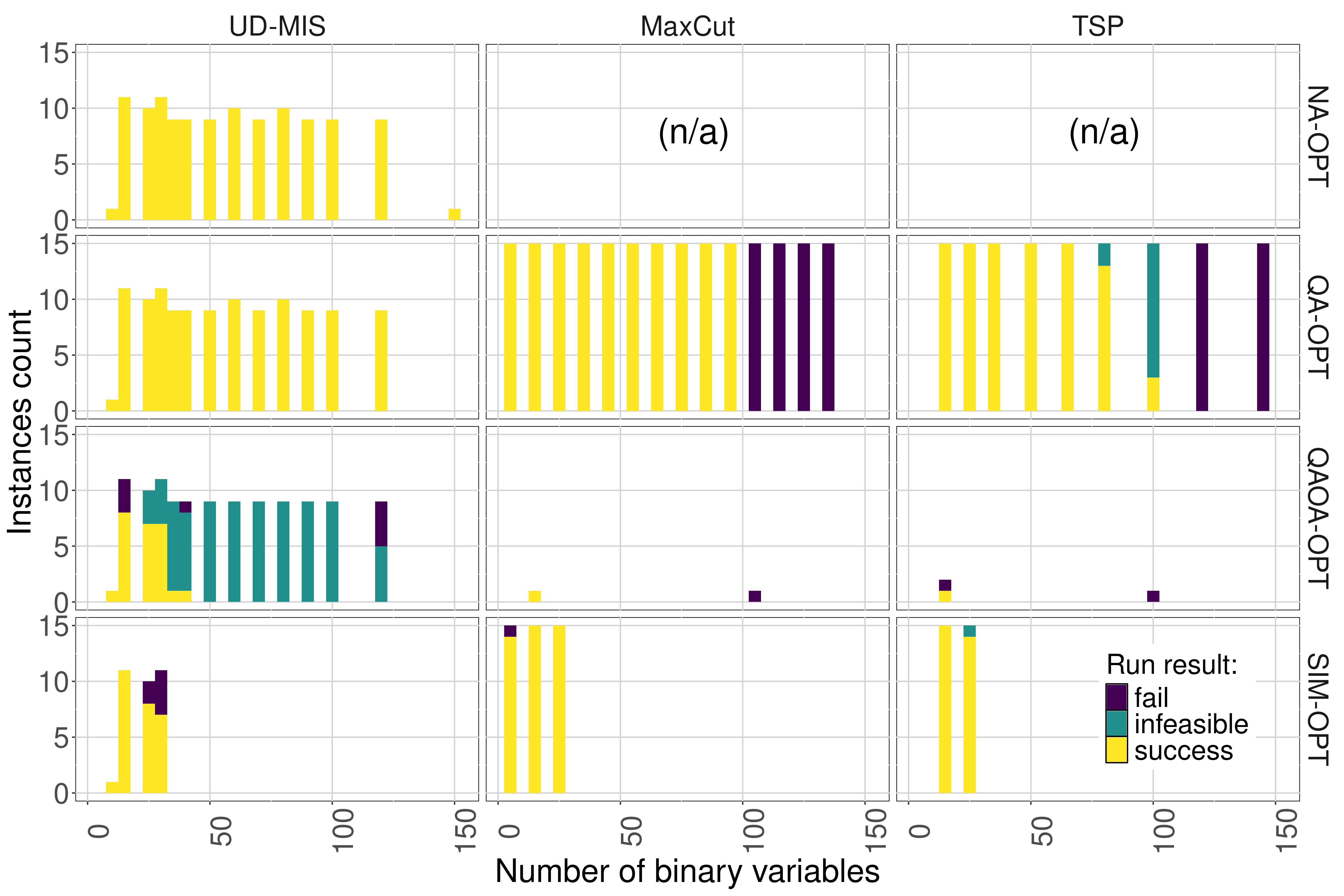
Baseline results.
Gurobi, as the classical baseline, found a feasible solution for all instances and is therefore not included in Figure 4. Specifically, all TSP instances were all solved to optimality with the largest runtime of about 15 minutes. Furthermore, the UD-MIS instances were all solved to optimality in under 1 second. Larger MaxCut instances were more time-consuming to solve. In total, 84% of MaxCut instances were solved with optimality gap of at most 5% (more than 99% with a gap of at most 10%). Note that there are specialized classical methods that might yield better runtimes (e.g., Rehfeldt et al., 2023 for MaxCut). Moreover, just imposing a time limit on the classical solver already yields a heuristic that takes only a fraction of time of the exact method, while ensuring comparable quality of solutions: For our selection of instances, Gurobi was very successful in finding good solutions early on, and spent significant amount of time on improving the bounds. (See also Supplement I.)
Performance metrics.
To evaluate the performance of each run, we consider the relative objective value deviation from the baseline and the relative runtime deviation from the baseline ,
| (15) |
respectively. Here, denotes the resulting objective value from the run of interest and its runtime. Analogously, denotes the best objective value found by Gurobi for the same instance (which is not necessarily the optimal solution for some MaxCut instances), and denotes the corresponding runtime. We presume here that for all considered instances.
Runtimes.
A runtime comparison of the considered approaches to Gurobi is presented in Figure 5(a). Each point represents a single run, and the tilted line in the top left corner reflects the situation where the compared runtimes are equal. For the comparably small problem instances of interest, the runtimes for quantum-powered approaches (if feasible) were mostly longer than the classical baseline (points below the tilted line). However, there is a small set of problem instances for which the runtime of Gurobi is longer than for the QA-OPT approach (points above the tilted line). For this subset of “hard” MaxCut instances, Gurobi required more than 20 seconds for a solution. The “hard” instances are all larger MaxCut instances, and investigating their structure in the context of OR applications might constitute a promising direction for further quantum optimization research. A detailed view of the “hard” instances is shown in Figure 5(b).
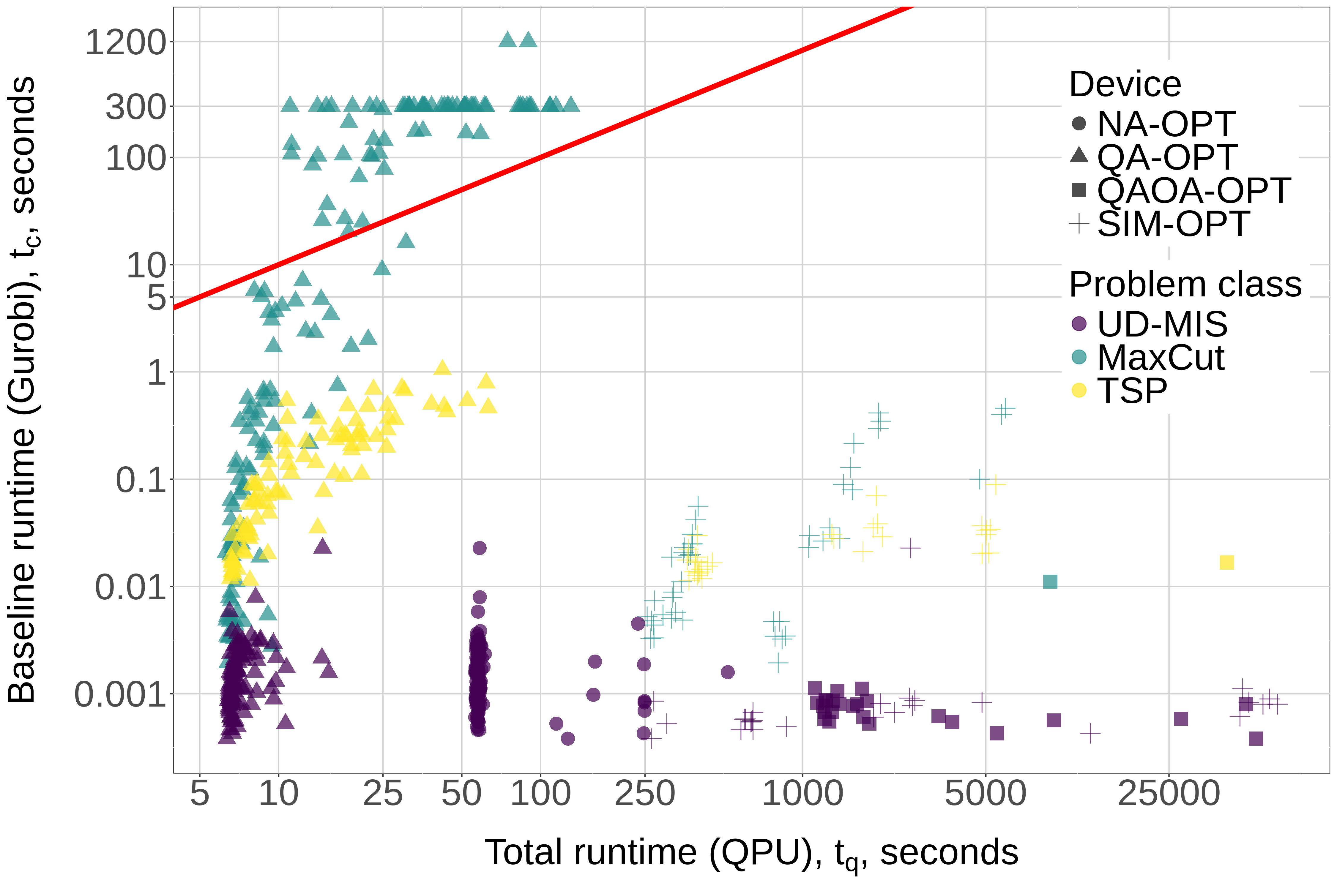
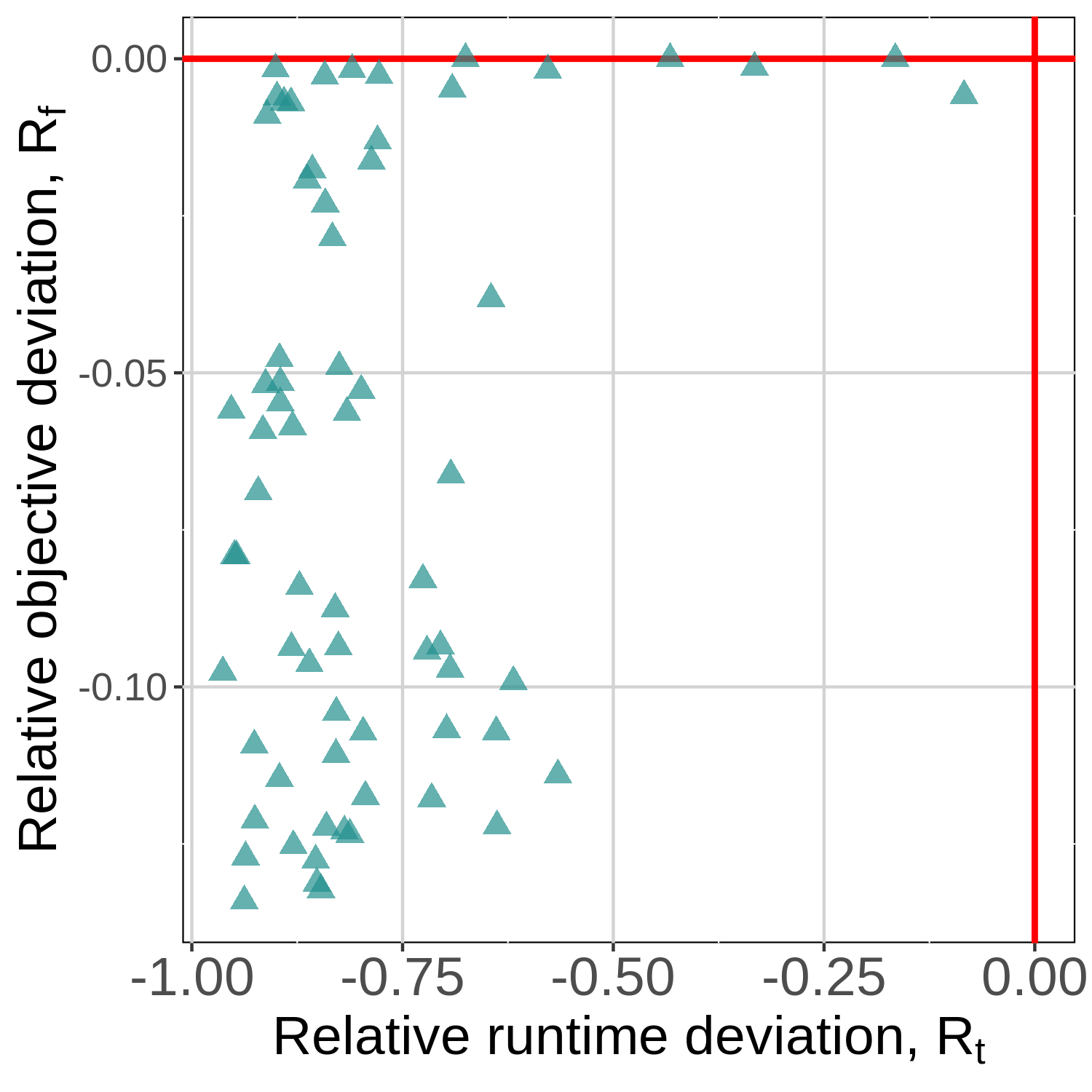
Objective values.
A comparison of the objective values from the quantum-powered approaches with the objective values from Gurobi is presented in Table 3. No quantum-powered run has a resulting objective value better than the corresponding Gurobi result. We observe that for both MaxCut and TSP, the quantum-powered approaches found many solutions within 25% of the Gurobi solutions. For the subset of “hard” MaxCut instances, Figure 5(b), where Gurobi required more than 20 seconds for a solution, the QA-OPT approach was able to find some solutions within 10--15% from the baseline objective in only half of the respective runtime.1313 13 The set of instances where Gurobi took more than 20 seconds coincided with the set of instances where QA-OPT took no more time than Gurobi. We refer to such instances as “hard.”
While the proportion of instances that were solved by QA-OPT no worse than Gurobi is comparable across problem classes, the share of instances with a gap within 5% or 10% for the UD-MIS problem is noticeably lower than that for MaxCut. This might be surprising at first glance, given that the QUBO matrices for UD-MIS instances are significantly less dense. Understanding this effect might constitute a possible direction for further research. One possible reason could be the different structure of constraints and their effects of the penalty terms. In particular, relatively small deviations of the solution in terms of the Hamming distances (number of bitflips) might lead to large relative changes in the objective value. Analysis of the solution landscapes in terms of Hamming distances and effects of coefficients normalization might therefore constitute reasonable first steps towards this direction.
Further, each independent set constraint corresponding to a single edge, when formulated as a penalty term, is still relatively local and does not require many interaction terms in the objective. Therefore, the embedding process in the context of QA-OPT approach turns out less problematic. Formulating and falsifying such hypotheses might constitute a viable line of further research. A more careful approach to benchmarking involving a quantum annealer is discussed by Lubinski et al. (2024).
For the NA-OPT approach, the structure of constraints might also play a role for the performance. As discussed in Section 3.1, the implementation of UD-MIS instances on neutral-atom devices requires not only a hardware-compliant problem graph, but also a suitable geometric arrangement of the atoms. These geometric considerations, which directly affect the realizability and accuracy of the problem encoding, remain an important practical aspect of the NA-OPT approach (Wurtz et al., 2023). The atom placement in our experiments was directly driven by the instance generation process. A more sophisticated exploration of alternative placement strategies encoding the same UD-MIS instance may serve as a strategy to further enhance performance. While such a study lies beyond our intention to provide an “out-of-the-box experience,” it could serve as a starting point for future research.
In general, studying which characteristics of problem instances make them more or less suitable for quantum-powered optimization constitutes a possible further research direction (Koch et al., 2025), and the set of problem instances presented here could serve as a starting point for such an analysis.
| Problem | Approach | Number of instance runs with relative objective deviations | ||||||||
| class | Total | within | within | within | no worse | |||||
| UD-MIS | NA-OPT | |||||||||
| QA-OPT | ||||||||||
| QAOA-OPT | ||||||||||
| SIM-OPT | ||||||||||
| MaxCut | QA-OPT | |||||||||
| QAOA-OPT | – | – | – | – | ||||||
| SIM-OPT | ||||||||||
| TSP | QA-OPT | |||||||||
| QAOA-OPT | – | – | – | – | ||||||
| SIM-OPT | ||||||||||
(a): For example, with the approach NA-OPT, we obtain feasible solutions for 117 UD-MIS instances. Out of these 117 runs, 93 (i.e., 79.5% of the total of 117) achieve a 25% deviation from the Gurobi objective, and so on.
Minor embeddings.
To conclude, we report two key aspects of the necessary embedding process within the QA-OPT approach. First, the runtime of a classical computer to find the embedding and, second, the number of physical qubits necessary to realize it. As explained in Section 3.2, the number of required physical qubits can exceed the number of variables of the underlying QUBO due to the introduction of chains. See Supplement H for an illustration of a toy MaxCut instance embedding.
We found in our experiments that the bounds on the necessary numbers of qubits presented in Lemma 2 and were not always tight, i.e., the heuristic algorithm used to find embeddings (Cai et al., 2014) performed better than the upper bound given in Lemma 2, with the specific results depending on the qubit connectivity required by the problem instances at hand. We quantified this effect by assessing the observed relation between the numbers of logical qubits (from the problem instance) and physical qubits (from the embedding) for the QA-OPT approach. Our statistical model, ordinary least squares regression, yields estimates for , where for MaxCut and TSP instances, and for UD-MIS instances in our dataset. (See Supplement D for further details.) This agrees to our expectation that the share of nonzero entries in the QUBO matrix scales differently for different problem classes (see Supplement A), which affects the embedding overhead.
The embedding process also entails significant (classical) runtime costs. In our case, it dominates the solution time for large enough TSP and MaxCut instances, as illustrated in Figure 6. For sparser UD-MIS instances with comparable numbers of binary variables, finding embeddings was relatively easy. While the embedding time varies with the number of binary variables in general, we did not scale the allotted annealing time. Therefore, for large and dense instances, up to 90% of the total runtime was spent trying to find an embedding, before starting the actual computation on the QC.
UD-MIS
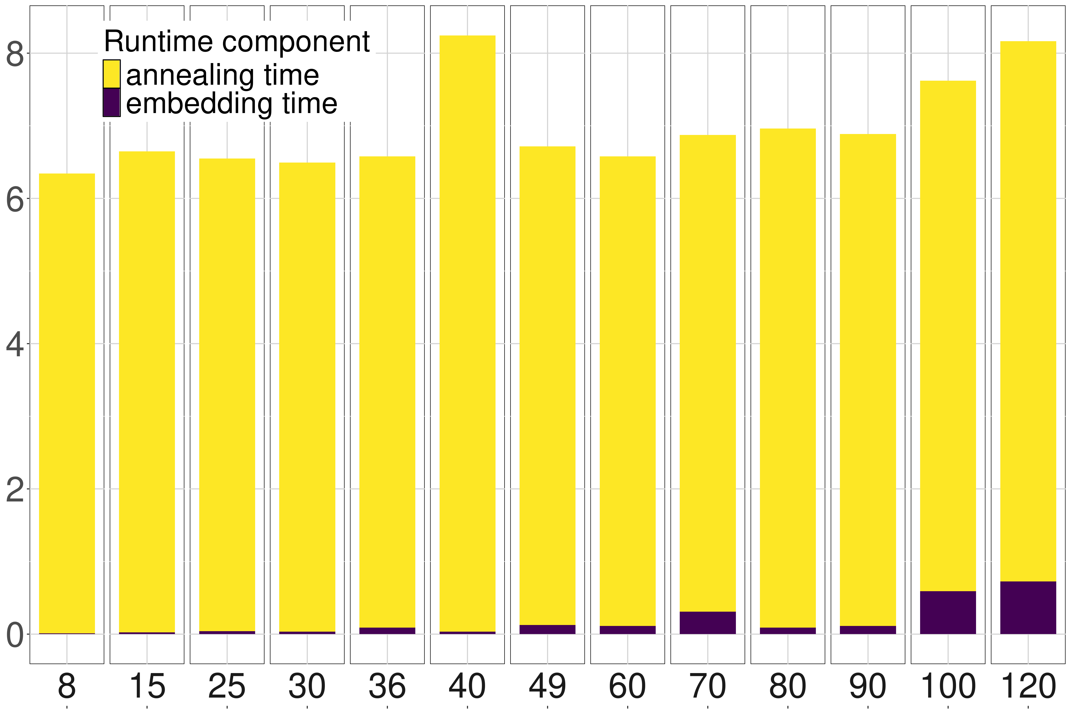
MaxCut
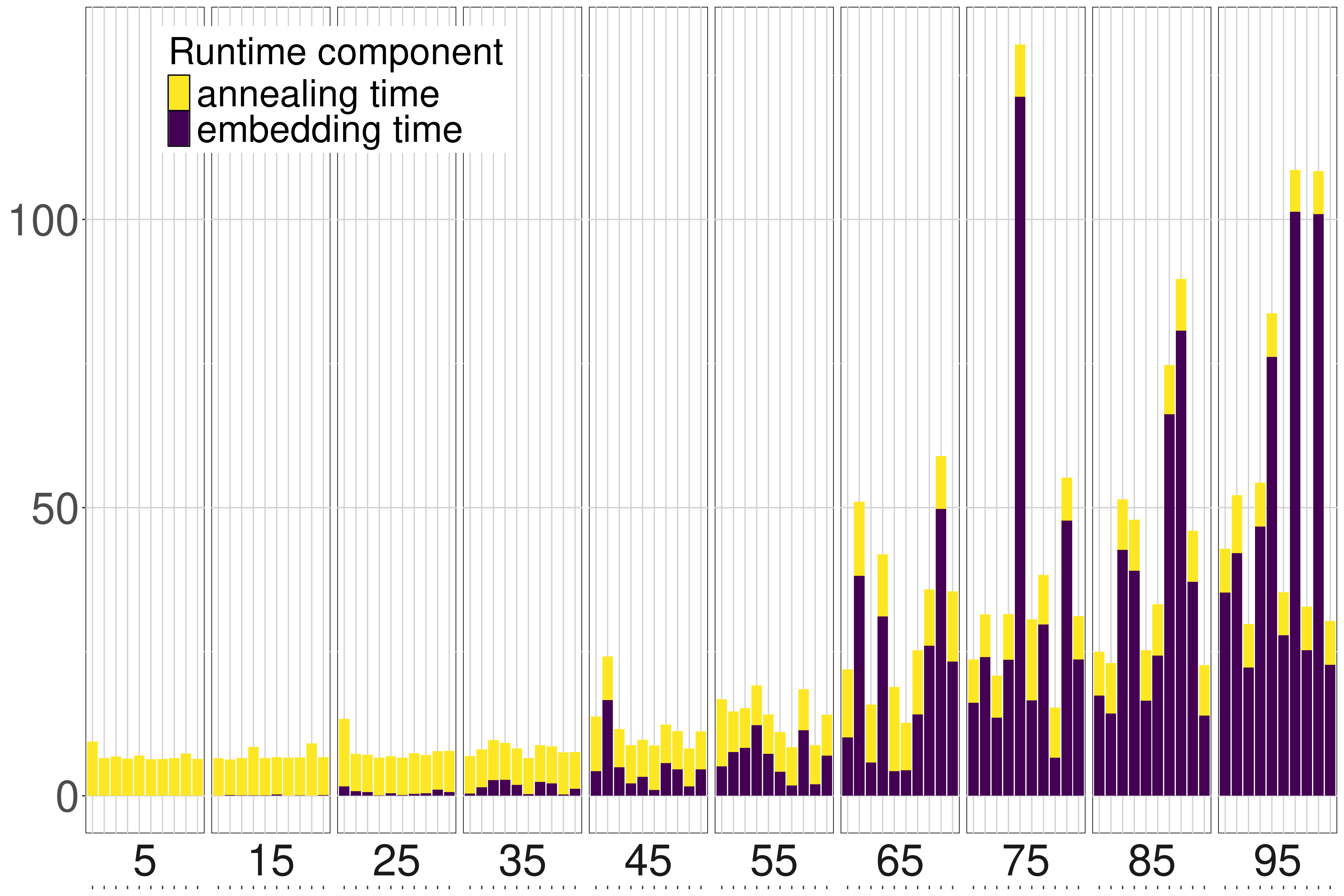
TSP

6 Conclusion
It is difficult to assess which of the currently available quantum computing architectures is superior for OR applications. Different quantum algorithms may have different hardware requirements, and device characteristics may affect the details of algorithm implementations. As a result, the development of hardware and the development of algorithms for practical applications go together. For this reason, rather than attempting to benchmark a broad collection of methods, we highlight three specific quantum-powered approaches to solve discrete optimization problems. Specifically, we consider two analog approaches, NA-OPT (solving UD-MIS with an analog QC based on neutral atom technology) and QA-OPT (solving QUBOs with a quantum annealer based on superconducting technology), as well as a digital approach, QAOA-OPT (solving QUBOs with a gate-based QC based on superconducting technology). The paper offers three groups of key contributions.
First, we provide a high-level overview of the relevant workflows, aiming at a general OR audience. To the best of our knowledge, this is the first attempt to describe several different quantum approaches in a uniform framework as sketched in Figure 2. We believe this effort will help motivate further involvement of the OR community into quantum optimization research. Fine-tuning of quantum algorithms and careful modeling of optimization problems may allow alternative quantum-powered solution strategies and therefore pose novel research opportunities (Blekos et al., 2024).
Second, we show that the required number of qubits for an optimization problem is not just a characteristic of the problem itself, but can be significantly affected by the chosen quantum technology, problem type, and the specific formulation, as listed in Tables 1 and . As discussed in Section 4, presenting new problem encodings is beyond the scope if this work, but we would like to emphasize the relevance of this issue in the context of quantum computing.
Third, we highlight the emergence of auxiliary optimization problems that arise in the course of applied quantum optimization in order to properly configure the respective quantum devices. Typically, such auxiliary problems are solved on a classical computer and could be a source for interdisciplinary collaborations between the quantum computing and OR communities. As a prototypical example, we discuss the embedding process within the QA-OPT approach and analyze the associated runtime and required number of physical qubits. We did not further explore the atom encoding step in the NA-OPT or the transpilation step in the QAOA-OPT, both of which represent distinct research directions. In general, improving heuristic methods for generating effective device configurations could enhance the practicality of all three quantum-powered approaches considered here.
Our numerical experiments have not shown a clear quantum advantage. The quality of the obtained numerical solutions depends on the problem class, but in general our classical baseline (solving an integer programming model using a state of the art commercial solver) outperformed the quantum-powered approaches, given enough time. However, even with all the restrictions of the available quantum devices, we were able to generate a collection of MaxCut instances that were hard enough for the classical solver, and for which we were able to obtain heuristic solutions from the quantum device with reasonable quality faster than using a classical solver, although it is not difficult to design classical heuristics that would outperform the quantum-powered approaches we discuss over our selection of instances. Our experiments highlight the obvious fact that the sparsity of the QUBO matrix affects the problem complexity, both for the classical baseline and the quantum-powered approaches.
We have found that the quantum-powered optimization approaches discussed in this paper provide very different user experiences. While they can be described in a largely unified framework, each presents its own unique strengths and challenges. For example, the QA-OPT approach typically produced feasible solutions for instances up to a certain size, provided suitable embeddings could be identified. However, finding embeddings for highly connected problem instances can become very difficult. The NA-OPT approach was even more robust in terms of results. On the other hand, it was more limited in terms of the number of qubits and required a representation of the problem as a UD-MIS, which quickly leads to infeasible resource requirements. Finally, the QAOA-OPT approach, while the most flexible for algorithm development, required the most effort to establish a reliable computational workflow for technical reasons. These differences highlight the value of continued exploration across all quantum computing architectures. Rather than prematurely favoring one technology over another, it is important to recognize that each may be well suited to different types of OR problems. Improving our understanding of their computational capabilities and identifying promising application domains remain important directions for future research.
7 Acknowledgements
The work was partially funded by the Research Initiative Quantum Computing for Artificial Intelligence (QC-AI). Access to quantum hardware was funded by the Fraunhofer Quantum Now program.
References
- Abbas et al. (2024) Abbas, A., Ambainis, A., Augustino, B., Bärtschi, A., Buhrman, H., Coffrin, C., Cortiana, G., Dunjko, V., Egger, D.J., Elmegreen, B.G., Franco, N., Fratini, F., Fuller, B., Gacon, J., Gonciulea, C., Gribling, S., Gupta, S., Hadfield, S., Heese, R., Kircher, G., Kleinert, T., Koch, T., Korpas, G., Lenk, S., Marecek, J., Markov, V., Mazzola, G., Mensa, S., Mohseni, N., Nannicini, G., O’Meara, C., Tapia, E.P., Pokutta, S., Proissl, M., Rebentrost, P., Sahin, E., Symons, B.C.B., Tornow, S., Valls, V., Woerner, S., Wolf-Bauwens, M.L., Yard, J., Yarkoni, S., Zechiel, D., Zhuk, S., Zoufal, C., 2024. Challenges and opportunities in quantum optimization. Nat. Rev. Phys. 6, 718–735. doi:10.1038/s42254-024-00770-9.
- Albash \BBA Lidar (2018) Albash, T., Lidar, D.A., 2018. Adiabatic quantum computation. Rev. Mod. Phys. 90, 015002. doi:10.1103/revmodphys.90.015002.
- Amazon Web Services (2020) Amazon Web Services, 2020. Amazon Braket. URL: https://aws.amazon.com/braket/.
- Applegate et al. (2006) Applegate, D.L., Bixby, R.E., Chvátal, V., Cook, W.J., 2006. The Traveling Salesman Problem: A Computational Study. volume 17 of Princeton Series in Applied Mathematics. Princeton University Press, Princeton. doi:10.1515/9781400841103.
- Au-Yeung et al. (2023) Au-Yeung, R., Chancellor, N., Halffmann, P., 2023. NP-hard but no longer hard to solve? Using quantum computing to tackle optimization problems. Front. Quantum Sci. Technol. 2, 1128576. doi:10.3389/frqst.2023.1128576.
- Baheri et al. (2022) Baheri, B., Guan, Q., Chaudhary, V., Li, A., 2022. Quantum noise in the flow of time: A temporal study of the noise in quantum computers, in: IEEE 28th Int. Symp. On-Line Testing and Robust System Design (IOLTS), pp. 1–5. doi:10.1109/IOLTS56730.2022.9897404.
- Barkoutsos et al. (2020) Barkoutsos, P.K., Nannicini, G., Robert, A., Tavernelli, I., Woerner, S., 2020. Improving variational quantum optimization using CVaR. Quantum 4, 256. doi:10.22331/q-2020-04-20-256.
- Bera et al. (2017) Bera, M.N., Acín, A., Kuś, M., Mitchell, M.W., Lewenstein, M., 2017. Randomness in quantum mechanics: philosophy, physics and technology. Rep. Prog. Phys. 80, 124001. doi:10.1088/1361-6633/aa8731.
- Blekos et al. (2024) Blekos, K., Brand, D., Ceschini, A., Chou, C.H., Li, R.H., Pandya, K., Summer, A., 2024. A review on quantum approximate optimization algorithm and its variants. Phys. Rep. 1068, 1–66. doi:10.1016/j.physrep.2024.03.002.
- Bolusani et al. (2024) Bolusani, S., Besançon, M., Bestuzheva, K., Chmiela, A., Dionísio, J., Donkiewicz, T., van Doornmalen, J., Eifler, L., Ghannam, M., Gleixner, A., Graczyk, C., Halbig, K., Hedtke, I., Hoen, A., Hojny, C., van der Hulst, R., Kamp, D., Koch, T., Kofler, K., Lentz, J., Manns, J., Mexi, G., Mühmer, E., Pfetsch, M.E., Schlösser, F., Serrano, F., Shinano, Y., Turner, M., Vigerske, S., Weninger, D., Xu, L., 2024. The SCIP Optimization Suite 9.0. Preprint. doi:10.48550/arXiv.2402.17702.
- Bombieri et al. (2025) Bombieri, L., Zeng, Z., Tricarico, R., Lin, R., Notarnicola, S., Cain, M., Lukin, M.D., Pichler, H., 2025. Quantum adiabatic optimization with Rydberg arrays: Localization phenomena and encoding strategies. PRX Quantum 6 2. URL: http://dx.doi.org/10.1103/PRXQuantum.6.020306, doi:10.1103/prxquantum.6.020306.
- Boothby et al. (2020) Boothby, K., Bunyk, P., Raymond, J., Roy, A., 2020. Next-generation topology of D-Wave quantum processors. Preprint. doi:10.48550/arXiv.2003.00133.
- Breu \BBA Kirkpatrick (1998) Breu, H., Kirkpatrick, D.G., 1998. Unit disk graph recognition is NP-hard. Comput. Geom. 9, 3–24. doi:10.1016/S0925-7721(97)00014-X.
- Bucher et al. (2025) Bucher, D., Stein, J., Feld, S., Linnhoff-Popien, C., 2025. IF-QAOA: A penalty-free approach to accelerating constrained quantum optimization. Preprint. doi:10.48550/arXiv.2504.08663.
- Cai et al. (2014) Cai, J., Macready, W.G., Roy, A., 2014. A practical heuristic for finding graph minors. Preprint. doi:10.48550/arXiv.1406.2741.
- Castelvecchi (2023) Castelvecchi, D., 2023. IBM releases first-ever 1,000-qubit quantum chip. Nature 624, 238. doi:10.1038/d41586-023-03854-1.
- Cerezo et al. (2021) Cerezo, M., Arrasmith, A., Babbush, R., Benjamin, S.C., Endo, S., Fujii, K., McClean, J.R., Mitarai, K., Yuan, X., Cincio, L., Coles, P.J., 2021. Variational quantum algorithms. Nat. Rev. Phys. 3, 625–644. doi:10.1038/s42254-021-00348-9.
- Chandarana et al. (2022) Chandarana, P., Hegade, N.N., Paul, K., Albarrán-Arriagada, F., Solano, E., del Campo, A., Chen, X., 2022. Digitized-counterdiabatic quantum approximate optimization algorithm. Phys. Rev. Research 4, 013141. doi:10.1103/physrevresearch.4.013141.
- Choi (2008) Choi, V., 2008. Minor-embedding in adiabatic quantum computation: I. The parameter setting problem. Quantum Inf. Process. 7, 193–209. doi:10.1007/s11128-008-0082-9.
- Clark et al. (1990) Clark, B.N., Colbourn, C.J., Johnson, D.S., 1990. Unit disk graphs. Discrete Math. 86, 165–177. doi:10.1016/0012-365X(90)90358-O.
- Codognet (2024) Codognet, P., 2024. Comparing integer encodings in QUBO for quantum and digital annealing: The travelling salesman problem, in: Sevaux, M., Olteanu, A.L., Pardo, E.G., Sifaleras, A., Makboul, S. (Eds.), Metaheuristics, Springer Nature Switzerland. pp. 262–267. doi:10.1007/978-3-031-62912-9_25.
- Creemers \BBA Armas (2025) Creemers, S., Armas, L.F.P., 2025. Discrete optimization: A quantum revolution? Eur. J. Oper. Res. 323, 378–408. doi:10.1016/j.ejor.2024.12.016.
- Crooks (2019) Crooks, G.E., 2019. Gradients of parameterized quantum gates using the parameter-shift rule and gate decomposition. Preprint. doi:10.48550/arXiv.1905.13311.
- D-Wave (2024) D-Wave, 2024. D-Wave Leap. URL: https://cloud.dwavesys.com.
- Dantzig et al. (1954) Dantzig, G., Fulkerson, R., Johnson, S., 1954. Solution of a large-scale traveling-salesman problem. J. Oper. Res. Soc. Am. 2, 393–410. doi:10.1287/opre.2.4.393.
- Das \BBA Chakrabarti (2005) Das, A., Chakrabarti, B.K., 2005. Quantum Annealing and Related Optimization Methods. Springer Science & Business Media. doi:10.1007/11526216.
- Dattani et al. (2019) Dattani, N., Szalay, S., Chancellor, N., 2019. Pegasus: The second connectivity graph for large-scale quantum annealing hardware. Preprint. doi:10.48550/arxiv.1901.07636.
- Dominguez et al. (2023) Dominguez, F., Unger, J., Traube, M., Mant, B., Ertler, C., Lechner, W., 2023. Encoding-independent optimization problem formulation for quantum computing. Front. Quantum Sci. Technol. 2 doi:10.3389/frqst.2023.1229471.
- Ebadi et al. (2022) Ebadi, S., Keesling, A., Cain, M., Wang, T.T., Levine, H., Bluvstein, D., Semeghini, G., Omran, A., Liu, J., Samajdar, R., Luo, X.Z., Nash, B., Gao, X., Barak, B., Farhi, E., Sachdev, S., Gemelke, N., Zhou, L., Choi, S., Pichler, H., Wang, S., Greiner, M., Vuletić, V., Lukin, M.D., 2022. Quantum optimization of maximum independent set using Rydberg atom arrays. Science 376, 1209–1215. doi:10.1126/science.abo6587.
- Ebadi et al. (2021) Ebadi, S., Wang, T.T., Levine, H., Keesling, A., Semeghini, G., Omran, A., Bluvstein, D., Samajdar, R., Pichler, H., Ho, W.W., Choi, S., Sachdev, S., Greiner, M., Vuletić, V., Lukin, M.D., 2021. Quantum phases of matter on a 256-atom programmable quantum simulator. Nature 595, 227–232. doi:10.1038/s41586-021-03582-4.
- Egger et al. (2021) Egger, D.J., Mareček, J., Woerner, S., 2021. Warm-starting quantum optimization. Quantum 5, 479. doi:10.22331/q-2021-06-17-479.
- Erdős \BBA Rényi (1959) Erdős, P., Rényi, A., 1959. On random graphs I. Publ. Math. Debrecen 6, 290–297. doi:10.5486/pmd.1959.6.3-4.12.
- Farhi et al. (2014) Farhi, E., Goldstone, J., Gutmann, S., 2014. A quantum approximate optimization algorithm. Preprint. doi:10.48550/arXiv.1411.4028.
- Farhi et al. (2000) Farhi, E., Goldstone, J., Gutmann, S., Sipser, M., 2000. Quantum computation by adiabatic evolution. Preprint. doi:10.48550/arXiv.quant-ph/0001106.
- Finnila et al. (1994) Finnila, A.B., Gomez, M.A., Sebenik, C., Stenson, C., Doll, J.D., 1994. Quantum annealing: A new method for minimizing multidimensional functions. Chem. Phys. Lett. 219, 343–348. doi:10.1016/0009-2614(94)00117-0.
- Fuchs \BBA Bassa (2024) Fuchs, F.G., Bassa, R.P., 2024. LX-mixers for QAOA: Optimal mixers restricted to subspaces and the stabilizer formalism. Quantum 8, 1535. doi:10.22331/q-2024-11-25-1535.
- Fuchs et al. (2022) Fuchs, F.G., Lye, K.O., Møll Nilsen, H., Stasik, A.J., Sartor, G., 2022. Constraint preserving mixers for the quantum approximate optimization algorithm. Algorithms 15, 202. doi:10.3390/a15060202.
- Garfinkel (1985) Garfinkel, R.S., 1985. Motivation and modeling, in: Lawler, E.L., Lenstra, J.K., Rinnooy Kan, A.H.G., Shmoys, D.B. (Eds.), The Traveling Salesman Problem. Wiley, Chichester, UK. Wiley Series in Discrete Mathematics & Optimization. chapter 2, pp. 17–36.
- Gilbert et al. (2024) Gilbert, V., Rodriguez, J., Louise, S., 2024. Benchmarking quantum annealers with near-optimal minor-embedded instances, in: 2024 IEEE Int. Conf. Quantum Computing and Engineering (QCE), IEEE. pp. 531–537. doi:10.1109/QCE60285.2024.00068.
- Glover et al. (2022) Glover, F., Kochenberger, G., Hennig, R., Du, Y., 2022. Quantum bridge analytics I: a tutorial on formulating and using QUBO models. Ann. Oper. Res. 314, 141–183. doi:10.1007/s10479-022-04634-2.
- Gomez-Tejedor et al. (2025) Gomez-Tejedor, A., Osaba, E., Villar-Rodriguez, E., 2025. Addressing the minor-embedding problem in quantum annealing and evaluating state-of-the-art algorithm performance. Preprint. doi:10.48550/arXiv.2504.13376.
- Gonzalez-Bermejo et al. (2022) Gonzalez-Bermejo, S., Alonso-Linaje, G., Atchade-Adelomou, P., 2022. GPS: A new TSP formulation for its generalizations type QUBO. Mathematics 10, 416. doi:10.3390/math10030416.
- Goswami et al. (2024) Goswami, K., Mukherjee, R., Ott, H., Schmelcher, P., 2024. Solving optimization problems with local light shift encoding on Rydberg quantum annealers. Phys. Rev. Research 6, 023031. doi:10.1103/physrevresearch.6.023031.
- Gottesman (2022) Gottesman, D., 2022. Opportunities and challenges in fault-tolerant quantum computation. Preprint. doi:10.48550/arXiv.2210.15844.
- Grange et al. (2023) Grange, C., Poss, M., Bourreau, E., 2023. An introduction to variational quantum algorithms for combinatorial optimization problems. 4OR 21, 363–403. doi:10.1007/s10288-023-00549-1.
- Grover (1996) Grover, L.K., 1996. A fast quantum mechanical algorithm for database search, in: Proc. 28th Annu. ACM Symp. Theory of Computing (STOC), ACM. pp. 212–219. doi:10.1145/237814.237866.
- Gurobi (2024) Gurobi, 2024. Gurobi Optimizer Reference Manual. Gurobi Optimization, LLC. URL: https://www.gurobi.com.
- Gyongyosi \BBA Imre (2019) Gyongyosi, L., Imre, S., 2019. A survey on quantum computing technology. Comput. Sci. Rev. 31, 51–71. doi:10.1016/j.cosrev.2018.11.002.
- Hadfield (2021) Hadfield, S., 2021. On the representation of Boolean and real functions as Hamiltonians for quantum computing. ACM Trans. Quantum Comput. 2, 18. doi:10.1145/3478519.
- Hadfield et al. (2019) Hadfield, S., Wang, Z., O’Gorman, B., Rieffel, E.G., Venturelli, D., Biswas, R., 2019. From the quantum approximate optimization algorithm to a quantum alternating operator ansatz. Algorithms 12, 34. doi:10.3390/a12020034.
- Hadfield et al. (2017) Hadfield, S., Wang, Z., Rieffel, E.G., O’Gorman, B., Venturelli, D., Biswas, R., 2017. Quantum Approximate Optimization with hard and soft constraints, in: Proc. 2nd Int. Workshop Post Moores Era Supercomputing, ACM. pp. 15–21. doi:10.1145/3149526.3149530.
- Hadfield (2018) Hadfield, S.A., 2018. Quantum Algorithms for Scientific Computing and Approximate Optimization. Ph.D. thesis. Columbia University. doi:10.7916/D8X650C9.
- Hangleiter \BBA Eisert (2023) Hangleiter, D., Eisert, J., 2023. Computational advantage of quantum random sampling. Rev. Mod. Phys. 95, 035001. doi:10.1103/revmodphys.95.035001.
- Harrow \BBA Montanaro (2017) Harrow, A.W., Montanaro, A., 2017. Quantum computational supremacy. Nature 549, 203–209. doi:10.1038/nature23458.
- Hauke et al. (2020) Hauke, P., Katzgraber, H.G., Lechner, W., Nishimori, H., Oliver, W.D., 2020. Perspectives of quantum annealing: methods and implementations. Rep. Prog. Phys. 83, 054401. doi:10.1088/1361-6633/ab85b8.
- Hoefler et al. (2023) Hoefler, T., Häner, T., Troyer, M., 2023. Disentangling hype from practicality: On realistically achieving quantum advantage. Commun. ACM 66, 82–87. doi:10.1145/3571725.
- Hua et al. (2023) Hua, F., Wang, M., Li, G., Peng, B., Liu, C., Zheng, M., Stein, S., Ding, Y., Zhang, E.Z., Humble, T., Li, A., 2023. QASMTrans: A QASM quantum transpiler framework for NISQ devices, in: Proc. SC’23 Workshops of Int. Conf. High Performance Computing, Network, Storage, and Analysis, ACM. pp. 1468–1477. doi:10.1145/3624062.3624222.
- IBM Quantum (2023a) IBM Quantum, 2023a. URL: https://quantum.ibm.com/.
- IBM Quantum (2023b) IBM Quantum, 2023b. IBM Quantum Documentation: Transpiler. IBM. URL: https://docs.quantum.ibm.com/api/qiskit/transpiler.
- Javadi-Abhari et al. (2024) Javadi-Abhari, A., Treinish, M., Krsulich, K., Wood, C.J., Lishman, J., Gacon, J., Martiel, S., Nation, P.D., Bishop, L.S., Cross, A.W., Johnson, B.R., Gambetta, J.M., 2024. Quantum computing with qiskit. Preprint. doi:10.48550/arXiv.2405.08810.
- Karp (1975) Karp, R.M., 1975. On the computational complexity of combinatorial problems. Networks 5, 45–68. doi:10.1002/net.1975.5.1.45.
- Karuppasamy et al. (2025) Karuppasamy, K., Puram, V., Johnson, S., Thomas, J.P., 2025. A comprehensive review of quantum circuit optimization: Current trends and future directions. Quantum Rep. 7, 2. doi:10.3390/quantum7010002.
- Katabarwa et al. (2024) Katabarwa, A., Gratsea, K., Caesura, A., Johnson, P.D., 2024. Early fault-tolerant quantum computing. PRX Quantum 5, 020101. doi:10.1103/PRXQuantum.5.020101.
- Kim et al. (2023) Kim, Y., Eddins, A., Anand, S., Wei, K.X., Van Den Berg, E., Rosenblatt, S., Nayfeh, H., Wu, Y., Zaletel, M., Temme, K., et al., 2023. Evidence for the utility of quantum computing before fault tolerance. Nature 618, 500–505. doi:10.1038/s41586-023-06096-3.
- Klug (2024) Klug, F., 2024. Quantum optimization algorithms in operations research: methods, applications, and implications. Preprint. doi:10.48550/arXiv.2312.13636.
- Koch et al. (2025) Koch, T., Neira, D.E.B., Chen, Y., Cortiana, G., Egger, D.J., Heese, R., Hegade, N.N., Cadavid, A.G., Huang, R., Itoko, T., Kleinert, T., Xavier, P.M., Mohseni, N., Montanez-Barrera, J.A., Nakano, K., Nannicini, G., O’Meara, C., Pauckert, J., Proissl, M., Ramesh, A., Schicker, M., Shimada, N., Takeori, M., Valls, V., Bulck, D.V., Woerner, S., Zoufal, C., 2025. Quantum optimization benchmark library – The Intractable Decathlon. Preprint. doi:10.48550/arXiv.2504.03832.
- Laurent (1997) Laurent, M., 1997. Max-Cut problem, in: Dell’Amico, M., Maffioli, F., Martello, S. (Eds.), Annotated Bibliographies in Combinatorial Optimization. Wiley, pp. 241–259. URL: https://www.wiley.com/en-ie/Annotated+Bibliographies+in+Combinatorial+Optimization-p-9780470860700.
- Lawler (1963) Lawler, E.L., 1963. The quadratic assignment problem. Manage. Sci. 9, 586–599. URL: https://www.jstor.org/stable/2627364, doi:10.1287/mnsc.9.4.586.
- Li et al. (2019) Li, G., Ding, Y., Xie, Y., 2019. Tackling the qubit mapping problem for NISQ-era quantum devices, in: Proc. 24th Int. Conf. Architectural Support for Programming Languages and Operating Systems, ACM. pp. 1001–1014. doi:10.1145/3297858.3304023.
- Lobe \BBA Lutz (2024) Lobe, E., Lutz, A., 2024. Minor embedding in broken chimera and derived graphs is NP-complete. Theor. Comput. Sci. 989, 114369. doi:10.1016/j.tcs.2023.114369.
- Lubinski et al. (2024) Lubinski, T., Coffrin, C., McGeoch, C., Sathe, P., Apanavicius, J., Bernal Neira, D., 2024. Optimization applications as quantum performance benchmarks. ACM Trans. Quantum Comput. doi:10.1145/3678184.
- Lucas (2014) Lucas, A., 2014. Ising formulations of many NP problems. Front. Phys. 2, 5. doi:10.3389/fphy.2014.00005.
- MacLennan (2009) MacLennan, B.J., 2009. Analog computation, in: Meyers, R.A. (Ed.), Encyclopedia of Complexity and Systems Science. Springer New York, New York, NY, pp. 271–294. doi:10.1007/978-0-387-30440-3_19.
- Markidis (2024) Markidis, S., 2024. What is quantum parallelism, anyhow? Preprint. doi:10.48550/arXiv.2405.07222.
- McGeoch \BBA Farré (2020) McGeoch, C., Farré, P., 2020. The D-Wave Advantage System: An Overview. Technical Report 14-1049A-A. D-Wave Systems Inc. URL: https://www.dwavesys.com/resources/white-paper/the-d-wave-advantage-system-an-overview/.
- Mermin (2007) Mermin, N.D., 2007. Quantum Computer Science. Cambridge University Press, Cambridge. doi:10.1017/CBO9780511813870.
- Miller et al. (1960) Miller, C.E., Tucker, A.W., Zemlin, R.A., 1960. Integer programming formulation of traveling salesman problems. J. ACM 7, 326–329. doi:10.1145/321043.321046.
- Morita \BBA Nishimori (2008) Morita, S., Nishimori, H., 2008. Mathematical foundation of quantum annealing. J. Math. Phys. 49 12. doi:10.1063/1.2995837.
- Mücke et al. (2025) Mücke, S., Gerlach, T., Piatkowski, N., 2025. Optimum-preserving QUBO parameter compression. Quantum Mach. Intell. 7 1. doi:10.1007/s42484-024-00219-3.
- Nannicini (2020) Nannicini, G., 2020. An introduction to quantum computing, without the physics. SIAM Rev. 62, 936–981. doi:10.1137/18M1170650.
- Nation \BBA Treinish (2023) Nation, P.D., Treinish, M., 2023. Suppressing quantum circuit errors due to system variability. PRX Quantum 4, 010327. doi:10.1103/PRXQuantum.4.010327.
- Nguyen et al. (2023) Nguyen, M.T., Liu, J.G., Wurtz, J., Lukin, M.D., Wang, S.T., Pichler, H., 2023. Quantum optimization with arbitrary connectivity using Rydberg atom arrays. PRX Quantum 4, 010316. doi:10.1103/PRXQuantum.4.010316.
- Nielsen \BBA Chuang (2010) Nielsen, M.A., Chuang, I.L., 2010. Quantum Computation and Quantum Information. 10th anniversary ed., Cambridge University Press, Cambridge, New York. doi:10.1017/CBO9780511976667.
- Padmasola et al. (2025) Padmasola, V., Li, Z., Chatterjee, R., Dyk, W., 2025. Solving the traveling salesman problem via different quantum computing architectures. Preprint. doi:10.48550/arXiv.2502.17725.
- Parekh (2023) Parekh, O., 2023. Synergies between operations research and quantum information science. INFORMS J. Comput. 35, 266–273. doi:10.1287/ijoc.2023.1268.
- Pelofske (2024) Pelofske, E., 2024. 4-clique network minor embedding for quantum annealers. Phys. Rev. Applied 21, 034023. doi:10.1103/PhysRevApplied.21.034023.
- Pelofske et al. (2020) Pelofske, E., Hahn, G., Djidjev, H., 2020. Advanced unembedding techniques for quantum annealers, in: Int. Conf. Rebooting Computing (ICRC), IEEE. pp. 34–41. doi:10.1109/ICRC2020.2020.00001.
- Pichler et al. (2018) Pichler, H., Wang, S.T., Zhou, L., Choi, S., Lukin, M.D., 2018. Quantum optimization for maximum independent set using Rydberg atom arrays. Preprint. doi:10.48550/arxiv.1808.10816.
- Preskill (2018) Preskill, J., 2018. Quantum computing in the NISQ era and beyond. Quantum 2, 79. doi:10.22331/q-2018-08-06-79.
- Rehfeldt et al. (2023) Rehfeldt, D., Koch, T., Shinano, Y., 2023. Faster exact solution of sparse MaxCut and QUBO problems. Math. Program. Comput. 15, 445–470. doi:10.1007/s12532-023-00236-6.
- Reinelt (1991) Reinelt, G., 1991. TSPLIB—a traveling salesman problem library. ORSA J. Comput. 3, 376–384. doi:10.1287/ijoc.3.4.376.
- Ruan et al. (2020) Ruan, Y., Marsh, S., Xue, X., Liu, Z., Wang, J., 2020. The Quantum Approximate Algorithm for Solving Traveling Salesman Problem. Comput. Mater. Contin. 63, 1237–1247. doi:10.32604/cmc.2020.010001.
- Sack et al. (2023) Sack, S.H., Medina, R.A., Kueng, R., Serbyn, M., 2023. Recursive greedy initialization of the quantum approximate optimization algorithm with guaranteed improvement. Phys. Rev. A 107, 062404. doi:10.1103/PhysRevA.107.062404.
- Sack \BBA Serbyn (2021) Sack, S.H., Serbyn, M., 2021. Quantum annealing initialization of the quantum approximate optimization algorithm. Quantum 5, 491. doi:10.22331/q-2021-07-01-491.
- Salehi et al. (2022) Salehi, O., Glos, A., Miszczak, J.A., 2022. Unconstrained binary models of the travelling salesman problem variants for quantum optimization. Quantum Inf. Process. 21, 67. doi:10.1007/s11128-021-03405-5.
- Scholten et al. (2024) Scholten, T.L., Williams, C.J., Moody, D., Mosca, M., Hurley, W., Zeng, W.J., Troyer, M., Gambetta, J.M., 2024. Assessing the benefits and risks of quantum computers. Preprint. doi:10.48550/arXiv.2401.16317.
- Serret et al. (2020) Serret, M.F., Marchand, B., Ayral, T., 2020. Solving optimization problems with Rydberg analog quantum computers: Realistic requirements for quantum advantage using noisy simulation and classical benchmarks. Phys. Rev. A 102, 052617. doi:10.1103/PhysRevA.102.052617.
- Shor (1997) Shor, P.W., 1997. Polynomial-time algorithms for prime factorization and discrete logarithms on a quantum computer. SIAM J. Comput. 26, 1484–1509. doi:10.1137/S0097539795293172.
- da Silva Coelho et al. (2022) da Silva Coelho, W., D’Arcangelo, M., Henry, L.P., 2022. Efficient protocol for solving combinatorial graph problems on neutral-atom quantum processors. Preprint. doi:10.48550/arXiv.2207.13030.
- Sinno et al. (2025) Sinno, S., Groß, T., Chancellor, N., Bhalgamiya, B., Sahoo, A., 2025. Optimized quantum embedding: A universal minor-embedding framework for large complete bipartite graph. Preprint. doi:10.48550/arXiv.2504.21112.
- Styer et al. (2002) Styer, D.F., Balkin, M.S., Becker, K.M., Burns, M.R., Dudley, C.E., Forth, S.T., Gaumer, J.S., Kramer, M.A., Oertel, D.C., Park, L.H., Rinkoski, M.T., Smith, C.T., Wotherspoon, T.D., 2002. Nine formulations of quantum mechanics. Am. J. Phys. 70, 288–297. doi:10.1119/1.1445404.
- Sugie et al. (2021) Sugie, Y., Yoshida, Y., Mertig, N., Takemoto, T., Teramoto, H., Nakamura, A., Takigawa, I., Minato, S.i., Yamaoka, M., Komatsuzaki, T., 2021. Minor-embedding heuristics for large-scale annealing processors with sparse hardware graphs of up to 102,400 nodes. Soft Comput. 25, 1731–1749. doi:10.1007/s00500-020-05502-6.
- Ulmann (2024) Ulmann, B., 2024. Beyond zeros and ones – analog computing in the twenty-first century. Int. J. Parallel, Emergent and Distrib. Syst. 39, 139–151. doi:10.1080/17445760.2023.2296672.
- Venegas-Andraca et al. (2018) Venegas-Andraca, S.E., Cruz-Santos, W., McGeoch, C., Lanzagorta, M., 2018. A cross-disciplinary introduction to quantum annealing-based algorithms. Contemp. Phys. 59, 174–197. doi:10.1080/00107514.2018.1450720.
- Waring et al. (2024) Waring, J.B., Pere, C., Beux, S.L., 2024. Noise aware utility optimization of NISQ devices. Preprint. doi:10.48550/arXiv.2402.08226.
- Wilson et al. (2020) Wilson, E., Singh, S., Mueller, F., 2020. Just-in-time quantum circuit transpilation reduces noise, in: 2020 IEEE Int. Conf. Quantum Computing and Engineering (QCE), IEEE. pp. 345–355. doi:10.1109/QCE49297.2020.00050.
- Wintersperger et al. (2023) Wintersperger, K., Dommert, F., Ehmer, T., Hoursanov, A., Klepsch, J., Mauerer, W., Reuber, G., Strohm, T., Yin, M., Luber, S., 2023. Neutral atom quantum computing hardware: Performance and end-user perspective. EPJ Quantum Technol. 10, 32. doi:10.1140/epjqt/s40507-023-00190-1.
- Wu et al. (2022) Wu, J., Lin, X., Guo, Y., Liu, J., Fang, L., Jiao, S., Dai, Q., 2022. Analog optical computing for artificial intelligence. Engineering 10, 133–145. doi:10.1016/j.eng.2021.06.021.
- Wurtz et al. (2023) Wurtz, J., Bylinskii, A., Braverman, B., Amato-Grill, J., Cantu, S.H., Huber, F., Lukin, A., Liu, F., Weinberg, P., Long, J., Wang, S.T., Gemelke, N., Keesling, A., 2023. Aquila: QuEra’s 256-qubit neutral-atom quantum computer. Preprint. doi:10.48550/arXiv.2306.11727.
- Wurtz et al. (2022) Wurtz, J., Lopes, P.L.S., Gorgulla, C., Gemelke, N., Keesling, A., Wang, S., 2022. Industry applications of neutral-atom quantum computing solving independent set problems. Preprint. doi:10.48550/arxiv.2205.08500.
- Zangeneh-Nejad et al. (2021) Zangeneh-Nejad, F., Sounas, D.L., Alù, A., Fleury, R., 2021. Analogue computing with metamaterials. Nat. Rev. Mater. 6, 207–225. doi:10.1038/s41578-020-00243-2.
- Zbinden et al. (2020) Zbinden, S., Bärtschi, A., Djidjev, H., Eidenbenz, S., 2020. Embedding algorithms for quantum annealers with Chimera and Pegasus connection topologies, in: Sadayappan, P., Chamberlain, B.L., Juckeland, G., Ltaief, H. (Eds.), High Performance Computing, Springer International Publishing. pp. 187–206. doi:10.1007/978-3-030-50743-5_10.
- Zhang et al. (2014) Zhang, D.J., Yu, X.D., Tong, D.M., 2014. Theorem on the existence of a nonzero energy gap in adiabatic quantum computation. Phys. Rev. A 90, 042321. doi:10.1103/physreva.90.042321.
- Zhao et al. (2022) Zhao, Y., Ye, Y., Huang, H.L., Zhang, Y., Wu, D., Guan, H., Zhu, Q., Wei, Z., He, T., Cao, S., Chen, F., Chung, T.H., Deng, H., Fan, D., Gong, M., Guo, C., Guo, S., Han, L., Li, N., Li, S., Li, Y., Liang, F., Lin, J., Qian, H., Rong, H., Su, H., Sun, L., Wang, S., Wu, Y., Xu, Y., Ying, C., Yu, J., Zha, C., Zhang, K., Huo, Y.H., Lu, C.Y., Peng, C.Z., Zhu, X., Pan, J.W., 2022. Realization of an error-correcting surface code with superconducting qubits. Phys. Rev. Lett. 129, 030501. doi:10.1103/PhysRevLett.129.030501.
- Zhou et al. (2020) Zhou, L., Wang, S.T., Choi, S., Pichler, H., Lukin, M.D., 2020. Quantum approximate optimization algorithm: Performance, mechanism, and implementation on near-term devices. Phys. Rev. X 10, 021067. doi:10.1103/PhysRevX.10.021067.
Supplementary materials
“Quantum Computing for Discrete Optimization:
A Highlight of Three Technologies ”
namesep= ,pairsep= and ,listsep=, ,lastsep= and ,tpairsep= and ,tlistsep=, ,tlastsep=, and ,notesep= ,rangesep= to ,type=book,Name-sg=Book,name-sg=book,Name-pl=Books,name-pl=books,type=part,Name-sg=Part,name-sg=part,Name-pl=Parts,name-pl=parts,type=chapter,Name-sg=Chapter,name-sg=chapter,Name-pl=Chapters,name-pl=chapters,type=section,Name-sg=Section,name-sg=section,Name-pl=Sections,name-pl=sections,type=paragraph,Name-sg=Paragraph,name-sg=paragraph,Name-pl=Paragraphs,name-pl=paragraphs,Name-sg-ab=Par.,name-sg-ab=par.,Name-pl-ab=Par.,name-pl-ab=par.,type=appendix,Name-sg=Appendix,name-sg=appendix,Name-pl=Appendices,name-pl=appendices,type=page,Name-sg=Page,name-sg=page,Name-pl=Pages,name-pl=pages,rangesep=–,rangetopair=false,type=line,Name-sg=Line,name-sg=line,Name-pl=Lines,name-pl=lines,type=figure,Name-sg=Figure,name-sg=figure,Name-pl=Figures,name-pl=figures,Name-sg-ab=Fig.,name-sg-ab=fig.,Name-pl-ab=Figs.,name-pl-ab=figs.,type=table,Name-sg=Table,name-sg=table,Name-pl=Tables,name-pl=tables,type=item,Name-sg=Item,name-sg=item,Name-pl=Items,name-pl=items,type=footnote,Name-sg=Footnote,name-sg=footnote,Name-pl=Footnotes,name-pl=footnotes,type=endnote,Name-sg=Note,name-sg=note,Name-pl=Notes,name-pl=notes,type=note,Name-sg=Note,name-sg=note,Name-pl=Notes,name-pl=notes,type=equation,Name-sg=Equation,name-sg=equation,Name-pl=Equations,name-pl=equations,Name-sg-ab=Eq.,name-sg-ab=eq.,Name-pl-ab=Eqs.,name-pl-ab=eqs.,refbounds-first-sg=,(,),,refbounds=(,,,),type=theorem,Name-sg=Theorem,name-sg=theorem,Name-pl=Theorems,name-pl=theorems,type=lemma,Name-sg=Lemma,name-sg=lemma,Name-pl=Lemmas,name-pl=lemmas,type=corollary,Name-sg=Corollary,name-sg=corollary,Name-pl=Corollaries,name-pl=corollaries,type=proposition,Name-sg=Proposition,name-sg=proposition,Name-pl=Propositions,name-pl=propositions,type=definition,Name-sg=Definition,name-sg=definition,Name-pl=Definitions,name-pl=definitions,type=proof,Name-sg=Proof,name-sg=proof,Name-pl=Proofs,name-pl=proofs,type=result,Name-sg=Result,name-sg=result,Name-pl=Results,name-pl=results,type=remark,Name-sg=Remark,name-sg=remark,Name-pl=Remarks,name-pl=remarks,type=example,Name-sg=Example,name-sg=example,Name-pl=Examples,name-pl=examples,type=algorithm,Name-sg=Algorithm,name-sg=algorithm,Name-pl=Algorithms,name-pl=algorithms,type=listing,Name-sg=Listing,name-sg=listing,Name-pl=Listings,name-pl=listings,type=exercise,Name-sg=Exercise,name-sg=exercise,Name-pl=Exercises,name-pl=exercises,type=solution,Name-sg=Solution,name-sg=solution,Name-pl=Solutions,name-pl=solutions\MH_if_boolean:nTshow˙only˙refs
This document supplements the main text by providing additional technical details. Note that to avoid confusion, labels (e.g., for the figures or tables) in these supplementary materials are prefixed with the letter “S.” For example, “Figure 5” refers to a figure in the main text, while “Figure S.5” points to a supplementary figure below.
The source code along with the data used to obtain the results presented in the paper can be downloaded from:
Corresponding technical documentation, including the discussion of relevant data formats and auxiliary programs, is available via:
A Instance generation
As presented in , we use randomized procedures to generate our collection of problem instances, which comprises three problem classes: Maximum independent set problem on a unit disk graph (UD-MIS), Weighted maximum cut problem (MaxCut), and Traveling salesperson problem (TSP). For each class, we create instances of varying sizes and problem structures with the following procedures:
- •
UD-MIS: To ensure that all generated instances are hardware-compliant (for Aquila), we consider the generation of unit disk graphs with nodes on a fixed grid. To that end, we use a fixed coordinate window , specifying the maximum integer values for each node coordinate on a two-dimensional plane. Then we create a grid of nodes with all possible integer coordinates for and . Finally, the nodes are deleted one by one11 1 The candidate for deletion being selected uniformly at random. until the desired total number of nodes is reached. The unit disk graph is then specified by this set of nodes and a real parameter as the unit disk radius. Variations in the coordinate window size allow us to generate instances of different node density on the coordinate plane, leading to different graph connectivity. Namely, for each studied problem size , we fix the window to to generate a set of points. We use three different values of to create different connectivity patterns in the grid of points22 2 Specifically, we used values of , , and — which are, respectively lower, higher, and comparable to the diagonal in the unit grid of . See the code documentation and specifically module MIS_inst.py for further implementation details., and repeat the procedure to generate three instances for each set of parameters. In addition to this procedure, we also build instances with hand-picked parameters for manual inspection: with a fixed value of , three different window sizes, and varying number of nodes between and . The provided unit disk radius for each instance is used as the blockade radius for Aquila within the NA-OPT approach.
- •
MaxCut: The collection of instances is created by generating a set of random graphs of different sizes using the Erdős-Rényi random graph model (Erdős \BBA Rényi, 1959), i.e., given nodes, each pair of nodes is connected by an edge with the probability . This procedure results in graphs of different connectivity depending on the parameter . Across the studied problem sizes , we generate graphs for . Weights are generated uniformly at random, within given limits.33 3 For each instance, we fix the maximum weight uniformly at random between and , and then pick edge weights uniformly at random between zero and . See code documentation and, specifically, module MWC_inst.py for specific implementation.
- •
TSP: We pick instances (uniformly) at random from TSPLIB (Reinelt, 1991), and sample the desired number of nodes from each one randomly, preserving edge weights.44 4 The original instances represent complete graphs, which, however, might contain fewer or more nodes than we require. In the former case we discard the instance, in the latter — pick a uniformly random subset of nodes of the necessary cardinality. See the code documentation and, specifically, module TSP_inst.py for further implementation details. Each sampling procedure results in a complete sub-graph of the original graph. Therefore, each selected TSPLIB instance yields a collection of TSP instances constituting complete graphs of the given sizes, with the same distances structure as compared to the original instance.
A summary of the instance sizes is shown in ??. For UD-MIS and MaxCut, example instances are shown in Figures S.1 and S.2, respectively.


A randomized instance generation allows us to consider different problem structures with respect to the resulting quadratic unconstrained binary optimization problem matrices, as visualized in Figure S.3. In particular, the generation procedure for MaxCut instances allows us to vary the density of QUBO matrix in our instance collection. The three values of the node connectivity parameter correspond to the three groups of MaxCut instances (dark triangles) in the plot. For large enough instances, these values approximately equal the shares of nonzero entries in the matrix. Our UD-MIS instances (dark circles) imply significantly less dense QUBO matrices, mostly due to the node degree restriction from the hardware requirements. TSP instances (light squares) occupy the middle position in terms of the matrix sparsity. In the following, we provide a brief theoretical illustration for the share of nonzero entries for each of the three problem classes of interest.

UD-MIS.
The QUBO matrix defined by formulation () has nonzero entries. If the node degree is bounded from above by some value that is independent of (as it is the case in our experiments), the total number of nonzero entries in is at most . Since the total number of entries in is , the share of nonzero entries is , decreasing as the problem scales up.
MaxCut.
The number of nonzero entries in matrix given by () is . Note that we deliberately generate instances with different node connectivity by varying node connectivity parameter in Erdős-Rényi model, taking values of , , and . If the number of edges is for some real number between zero and one, the share of nonzero entries in will constitute:
as the problem scales up with fixed . Namely, the share of nonzero entries in will approach the parameter used during the instance generation, as the number of nodes grows.
TSP.
The number of nonzero entries in the matrix defined in formulation () is in , out of entries in in total, and hence the share of nonzero entries belongs to .
B On the choice of penalty coefficients for QUBO formulations
Let us briefly revisit the choice of the penalty coefficients (denoted ) that we used to formulate QUBO instances in ??. Specifically, for each of the problem classes under consideration, we create an equivalent QUBO formulation, at least in the sense that optimal solutions of the original problem and the QUBO coincide.
- •
UD-MIS (Section ??, page ). Formulation () is equivalent to () for , since in this case a single independent set constraint violation ( for some ) makes this infeasible solution worse than a trivial feasible solution of .
- •
MaxCut (Section , page ). We discuss a natural quadratic formulation that does not involve penalty terms.
- •
TSP– (Section , page ). For both families of constraints, it suffices to set the penalty term to . Assume for a contradiction that there is an optimal solution that violates some constraint. If there is a node of degree whose neighbors all have degree , then replace this star by an arbitrary cycle through the set of involved vertices. This adds at most new edges and reduces the penalty of vertices. If there is a node of degree with a neighbor of degree , then removing the edge will reduce the penalty of and add the penalty for , while losing some positive cost . Assume now that all nodes have degree . If there are at least two nodes of degree smaller than , we can add an edge between them, while reducing the penalty by at least . If there is a single node of degree , then this node must have degree and all other nodes have degree . Then replacing an arbitrary edge by the edges and inserts two edges, and reduces the penalty twice. When all degree constraints are satisfied, then the solution is a union of cycles. For any two cycles, we can merge the two cycles by replacing two edges by two potentially longer edges, while correcting two violated subtour constraints, which reduces the penalty by at least .
- •
TSP– (Section , page ). In the penalty terms corresponding to the in-degree and out-degree constraints, we can still use the penalty by a similar argument as for the formulation. For the node ordering constraints, we can use the penalty . If there is a violation of an ordering constraint, this gives the possibility to have a subtour. This can be repaired by replacing two edges by two other edges. Hence, for the selected , such a merge reduces the objective value.
- •
TSP– (Section , page ). One specific value to ensure the equivalence is : In this case, violation of a single constraint makes the objective value larger (worse) than any of the feasible solutions.
C Required number of logical qubits for the QUBO formulation of TSP
We derive the result of ??, stating the necessary number of logical qubits for the QUBO reformulation of the TSP integer program (). This formulation involves binary variables only, but we still need to introduce penalty terms in order to transform it to an equivalent QUBO. The equality constraints can be directly translated into quadratic penalty terms: For each , the constraint induces the term in the QUBO objective function, where must be sufficiently large (e.g., ) to separate feasible and infeasible solutions in terms of the objective values. Inequality constraints () have to be converted to equalities by introducing integer slack variables. So, we replace every inequality constraint of the form
with the corresponding pair of constraints
This transformation introduces new integer variables , and we further substitute them with their binary representations. For every subset with the sum can take values between (if no two nodes from are visited consecutively) and (if all nodes from are visited consecutively). Therefore, we need binary variables for , so that we replace by , which can take all values between and . After this replacement, we can again derive quadratic penalty terms of the form
for large enough.
Therefore, for a Dantzig-Fulkerson-Johnson model, we have a corresponding QUBO with binary variables and penalty terms in the objective. To calculate the number of slack variables more precisely, note that we have constraints with slack at most two, constraints with slack at most three, and so on. The resulting number of slack variables is then
| if is odd, | |||||
| if is even. |
Therefore, we arrive at the desired result: When applying the standard procedure to reformulate the Dantzig-Fulkerson-Johnson model (), as a QUBO, the result has
binary variables. The first summand here gives the number of binary variables in the integer linear program. The next two summands give the number of new binary variables to represent the possible slacks. They generalize the two terms given above for odd or even and are derived by summing over all considered subset sizes and taking the number of such subsets times the necessary number of binary variables to represent the possible slack.
D Regression model for physical qubit requirements
In Figure S.4, we present the observed relation between the numbers of logical qubits (from the problem instance) and physical qubits (from the embedding) for the QA-OPT approach. Each point in the figure represents a solved instance, with random horizontal jitter added for visibility and the color and shape indicating the problem class. Both axes are on a natural logarithm scale. The dashed lines represent ordinary least squares regression in logarithmic scale.
To perform this regression, consider first a model equivalent to the power law for the number of physical qubits used after embedding as a function of the number of variables in the original QUBO model , i.e., hypothesizing that . Taking the logarithm of both parts suggests the following statistical model:
| (1) |
which depends on two parameters, the slope and the constant offset , and where the error term captures the discrepancies of the predicted values with the true values . This model can be fitted to our embedding data, logarithms of the number of physical qubits and logarithms of the respective numbers of binary variables, by minimizing the sum of squared errors using the ordinary least squares regression technique (Dalgaard, 2008). The resulting standard summary table for the model is shown in Table S.1.
| Dependent variable: in different regressions | |||
| UD-MIS | MaxCut | TSP | |
| : | |||
| (0.020) | (0.023) | (0.012) | |
| 0.316∗∗∗ | 1.652∗∗∗ | 1.626∗∗∗ | |
| (0.080) | (0.085) | (0.044) | |
| Observations | 116 | 150 | 105 |
| R2 | 0.964 | 0.978 | 0.996 |
| Adjusted R2 | 0.964 | 0.978 | 0.996 |
| Residual Std. Error | 0.139 (df = 114) | 0.243 (df = 148) | 0.072 (df = 103) |
| F Statistic | 3,064.768∗∗∗ | 6,679.321∗∗∗ | 25,468.300∗∗∗ |
E Computational workflows summary
Details for the three key steps of the computational workflow mentioned in ?? are summarized in Section E. First, the discrete optimization problem at hand must be reformulated into a suitable problem class: NA-OPT admits only UD-MIS, while QA-OPT and QAOA-OPT allow only QUBO. Then, the quantum computer (QC) and classical host machine (defining the computational framework) need to be configured. The quantum device configuration is usually prepared in a device-independent way, and then translated into the language of device-specific instructions. Different technologies require different amounts of computational overhead for this step. For the machines from IBM and QuEra, device configuration is relatively straightforward (depending on how much optional hardware-dependent optimization of the instructions is considered), while the D-Wave quantum annealer configuration involves a computationally difficult task related to graph embedding. Finally, the solution step is different across the three technologies. The neutral-atom-based device and the quantum annealer function in a similar (analog) mode, where the initial state is prepared, then a pre-defined evolution schedule is executed, and the result is read out. This process is repeated multiple times to obtain a distribution of solutions and try to alleviate the possible errors due to hardware limitations. Quantum approximate optimization algorithm (QAOA), on the other hand, is a variational quantum algorithm (VQA), a hybrid quantum-classical method. As such, its computation stage is different as it comprises a classical outer black-box optimization loop. However, after the solution is found, the processing is usually similar: the quantum state corresponding to the best found ansatz parameters is constructed and measured multiple times to obtain a sample of solutions to the original problem.
Key high-level steps of the computational workflow. Step NA-OPT QA-OPT QAOA-OPT 0) Formulation The problem is reformulated as UD-MIS a. The problem is reformulated as QUBO b. CONFIGURATION 1) QC setup Describing the initial state and key parameters of the quantum device: 1.1) Device-independent configuration Prepare problem-dependent spatial configuration for the atoms (the atoms array) and define the blockade radius. Set up annealing time. Design the quantum circuit (ansatz): • derive the problem-specific circuit form, • choose circuit depth. 1.2). Device-dependent configuration Translate the setup to physical device commands (automatically). Embedding: map logical qubits to the device nodes: • choose required “chain strength”, • find the mapping. The circuit is “transpiled” for the specific device: • map the gates to device-native gates, • add SWAP gates to ensure necessary qubit connectivity. 2) Framework parameters. • Set up the system evolution schedule. • Choose the number of shots. • Choose the number of shots (sample size), • implement the objective calculation procedure. • Choose initial circuit parameters, • implement objective function estimation, • set up a classical solver to find parameters. SOLUTION / PROCESSING 3) Computation Candidate solutions are sampled from the multiple shots of the QC. During each step: • prepare and initialize the device, • realize the evolution schedule, • sample a (single) solution. Candidate solutions are sampled from the multiple shots of the QC, each one comprising the following steps: • prepare and initialize the device, • anneal (converges the state to a low-energy one), • sample a (single) solution. • Given the circuit parameters, the QC is set up to output a candidate solution. • An auxiliary objective is set up as a function that takes circuit parameters, samples candidate solutions from the QC, and returns the QUBO objective. • A classical black-box optimizer searches for circuit parameter values that minimize the auxiliary objective, iteratively querying the QC. • A set of solutions is sampled from multiple shots from the QC, given the best circuit parameters found. 4) Post-processing Recover maximum independent set problem (MIS) solution(s): e.g., the most frequently sampled one. Recover QUBO solution(s): broken chains resolved (e.g., majority vote) QUBO solution for each shot. Recover QUBO solution(s), analyze convergence data.
- a
A weighted version of the problem and the respective maximum-weight independent set problem on a unit disk graph (UD-MWIS) reformulation (Nguyen et al., 2023) can also be used, if atom-specific detuning is allowed by the hardware.
- b
The conversion to QUBO (e.g., incorporating constraints, integer variables etc.) can be automatized to some extent by existing software tools.
F Summary of the different runs across instances
Our experimental setup involves an exploration phase, in which we test the feasibility of our approaches with regard to the proposed instance generation methods. Key information regarding the considered quantum hardware is summarized in Section F.
[t] Quantum hardware used for our quantum-powered approaches. Hardware Technology Qubits Used in approach References Aquila neutral-atom, analog NA-OPT Wurtz et al. (2023) Advantage superconducting, analog, chip v4.1 (a) QA-OPT McGeoch \BBA Farré (2022) ibm_cusco, superconducting, gate-based, QAOA-OPT IBM Quantum (2023), ibm_nazca chip family Eagle Chow et al. (2021)
- a
Device topology contains physical qubits, out of which at least must be available, according to the referenced technical report. The exact number depends on the specific device configuration and calibration, and may vary over time.
Calculations for some of the instances were repeated several times, to possibly obtain a feasible solution, or for technical reasons related to the interactions with the remote machines. A summary of all attempts is presented in Figure S.5. Each bar corresponds to a single instance, and counts correspond to the number of times the respective instance of the given type (in columns) was solved by each approach (in rows). Colors mark the run resultsm i.e., whether we were able to retrieve a feasible solution, only infeasible ones, or no solutions at all. The instances are sorted by size in the number of QUBO variables for each of the three problem classes, which is summarized into three groups (no more than 25 variables, between 26 and 100, and more than 100 variables) for readability.
For our analysis in the main text of the paper, we select one run per instance (which is summarized in ??), as follows. If we were able to obtain a feasible solution, we used the latest run that yielded one. Otherwise, we used the latest run among those that yielded at least an infeasible solution, or just the latest run if all of them failed.
G Example outputs from QCs
Typically, the output of a QC constitutes a sequence of bitstrings, each of which is obtained from a single shot.55 5 The number of shots is a parameter chosen at the configuration step. In our experiments, we aim for a sufficiently large number of shots, which still maintains reasonable total runtimes. For quantum optimization, each bitstring can usually be transformed into a binary solution vector of the considered optimization problem. For demonstration purposes, we present exemplary QC outputs in the following for the different quantum-powered approaches, i.e., QA-OPT, NA-OPT, and QAOA-OPT (including SIM-OPT).
QA-OPT.
Figure S.6 summarizes three output examples for the D-Wave device Advantage in our experiment. Each bar represents a single solution, “solution count” denotes the number of times this solution was sampled, and “energy” reflects the objective representation for the solution within the QC (which is an actual energy of the physical system in the corresponding state). “QUBO objective” presents an objective value calculated from a QUBO formulation, and ‘‘original objective’’ corresponds to the objective for the original problem.66 6 For feasible solutions, the latter two might differ only in sign, and no original objective values correspond to infeasible solutions. Thick horizontal line in the bottom panel represents the optimal objective value. The panel entitled ‘‘ch. breaks’’ represents the share of chain breaks---a measure of the quality of the measured solution.77 7 Chain breaks appear only for the largest instance in the figure.
We see a varying quality of the representation for the true objective with the quantum state. The top panel of Figure S.6 shows a typical “favorable case:” all the solutions are feasible (there are no feasibility constraints for MaxCut), and most of the sampled solutions are optimal or close to optimal. The middle panel, highlighting a five-nodes TSP instance with internal ID TSP53 (having binary variables in the QUBO), paints a more mixed picture. Most of the sampled solutions were feasible (although not all), and the algorithm was able to find a true optimum. However, it was not the most frequently sampled solution. The bottom panel presents an even more unfavorable case of a larger TSP with ID TSP82 and 49 QUBO variables, an 8-node TSP instance. First of all, most of the sampled solutions were actually infeasible for the original problem (hence, representing significantly suboptimal solutions to the corresponding QUBO). The solution frequency profile is not very pronounced, without clear maxima and most of the solutions sampled once or twice. The quality of the solution is worse, and there is a strictly positive absolute gap between the best found solution and a true optimum.
NA-OPT.
A similar situation is illustrated in Figure S.7 for the Aquila device. Again, the top panel represents a relatively favorable situation where more than half of the solutions are feasible, and the most frequently sampled one corresponds to a true optimum. In the middle panel, a significant number of solutions were sampled one or two times, but the frequency profile still has a maximum around a true optimal solution. The bottom panel represents yet another instance (which is approximately 4 times as large as the one corresponding to the top panel), and here we see a completely flat frequency profile of the sample: each solution was sampled exactly once. Such a difference in output quality is somewhat surprising, as the three instances mentioned here, Figure S.8, are very close in terms of the structure and in fact represent different numbers of similar, but unrelated UD-MIS problems, which are solved in parallel within a single shot. This highlights the fact that quantum-powered algorithms are complex and sometimes might require additional fine-tuning. Some “best practices” and practical considerations aiming specifically at the Aquila device are discussed by Wurtz et al. (2023).

QAOA-OPT and SIM-OPT.
Outputs for the same three instances from Figure S.8 on the IBM device ibm_nazca and a noise-free simulator are presented in Figure S.9. For these instance sizes, the simulator was able to find more feasible solutions, but overall the picture is the same. The smallest instance, UDMIS1TG, yields a reasonable solution frequency profile. Approximately doubling the number of variables results in most of the solutions being sampled once or twice, and doubling the number of variables again yields a completely flat frequency profile ( different solutions sampled, out of attempts), with noticeable number of infeasible solutions (more so for the quantum device in comparison with the simulator). In this direct comparison (based on our naive implementations), we find that the NA-OPT approach, while offering less flexibility than the QAOA-OPT approach, leads to better solutions for the considered UD-MIS instances.
H D-Wave embeddings: Chimera and Pegasus topology graphs
The topology graphs of D-Wave quantum annealers are intersection graphs of axis-parallel segments. An example, the so-called Chimera topology is shown in Figure S.10: the top left panel shows the intersecting segments (thick lines), where intersections of two neighboring horizontal or vertical qubits are represented by thin lines between them. The resulting topology graph is shown in the top right panel.
One safe way to obtain an embedding of the QUBO graph into is to search for an embedding of a clique into , which allows realizing all possible interactions. The problem of finding the largest clique minor in a broken topology graph is fixed-parameter tractable in the number of broken qubits (Lobe et al., 2021), i.e., it can be solved exactly with running time polynomial in the size of the topology graph (but exponential in the number of broken qubits). In this paper, for our upper bounds on the number of physical qubits required, we consider clique embeddings into the non-broken Pegasus graph, described below. In practice, broken qubits may turn these embeddings invalid and lead to a larger number of needed qubits, but on the other hand, the graphs resulting from our application problems are usually rather sparse, which allows for a significant reduction of qubits required as compared to our bound, which is confirmed by our experimental results, see ??.
To explain the clique embedding, we first consider the Chimera topology, shown in Figure S.10, which was used by a previous generation of D-Wave devices. It consists of eight-qubit cells, tiled vertically and horizontally, and connected to each other as presented in the top right panel of Figure S.10. Each cell constitutes a complete bipartite graph with four nodes on each side, denoted . The nodes from one of the bipartition classes (“horizontal qubits”, corresponding to horizontal segments) are connected to their counterparts in the horizontally neighboring cells, while the nodes from the other bipartition class (“vertical qubits”) are connected to the vertically neighboring cells. Every node has degree at most , which makes it in particular necessary to use multiple nodes (i.e., physical qubits) to represent any variable interacting with more than six other variables. Choi (2011) described a variant of clique embedding where always four chains are grouped together and each realizes the interactions within one such group or between two such groups (Klymko et al., 2013; Boothby et al., 2016; Date et al., 2019, see also). For example, in Figure S.10, a quadruple of binary variables, such as , is involved in five cells: one modeling the interactions within the quadruple and four for the interactions with each of the other variable quadruples. Distinct quadruples are represented by different colors in the figure; the high-level logic is shown in the bottom panel.

The topology graph of the Advantage device, the so-called Pegasus graph (Boothby et al., 2020; Dattani et al., 2019; D-Wave, n.d.), consists of three Chimera graphs with additional connections, see Figure S.11.
Each inner node has, in addition to the six incident edges from its Chimera graph, one extra edge to a neighboring node in its cell (breaking the bipartiteness) and eight edges to nodes from the other two Chimera graphs, giving a total node degree of . The connections between different Chimera graphs within the Pegasus graph are designed in a way that combining the Chimera embeddings of three cliques yields an embedding of (with some caution at the boundaries). This means that in order to embed a clique of logical qubits, we can subdivide this into three cliques of size and embed each into a Chimera consisting of -cells, resulting in cells in total, while an embedding into a single Chimera graph would require cells. Hence, (ignoring boundary effects), the number of required physical qubits to embed a clique into the new graph is divided by three. For either of the two topology graphs, an arbitrary QUBO with variables can thus be encoded using physical qubits, although with different hidden constants. Pelofske (2023) provides a detailed comparison of D-Wave’s device topologies. The exact number for Pegasus is given in the following lemma.
Lemma S.1 (Boothby et al., 2020).
For every the clique is a minor of a Pegasus graph consisting of nodes corresponding to physical qubits.
This result immediately gives us that if we want to embed logical qubits, then we can apply the lemma to , resulting in at most physical qubits for a connected QUBO instance, as presented in ??.
As outlined in ??, in our experiments the embeddings were calculated heuristically using the standard procedure offered by D-Wave. For example, the actual embedding for instance MWC3, a small MaxCut instance, is presented in Figure S.12. Specifically, the complete graph with five nodes was embedded into a subgraph of Pegasus topology comprising six, and not nodes: The variable indexed by in the figure is represented by a chain of two nodes in the device graph. Across our collection of instances, we needed slightly less than quadratically many physical qubits, which depended on the problem structure (see ??). Finding embeddings was very resource-intensive for larger instances, and constructing fast and reasonably effective heuristic algorithms might constitute an interesting direction for further research. While discussing the embeddings in more detail is beyond the scope of this article, we refer the reader to the works mentioned in ?? devoted to the topic for more details and remark that the embeddings for our considered problem instances are available for further analysis in the materials accompanying the paper (in the folder run_logs/dwave/embeddings).
Another representation of the experimental results that shows the annealing time and embedding time separately is given in Figure S.13. The left panel presents annealing time in seconds (without the embedding), while the embedding time shares across all considered instances are summarized in the right panel.


I On baseline model selection
Since numerical benchmarking is not the primary focus of this paper, we aimed to select baseline models that are as simple as possible while reflecting a natural first choice from the perspective of an Operations Research scientist. In this section, we elaborate further on our selection.
For TSP, many ways to model the problem are known, and many algorithms exist, including exact, approximate, and heuristic approaches (Lawler et al., 1985; Jünger et al., 1997). We consider three well-known alternative formulations: Dantzig-Fulkerson-Johnson (DFJ), Miller-Tucker-Zemlin (MTZ), and quadratic assignment problem (QAP). Since the DFJ formulation has an exponential number of constraints, we choose the next simplest linear model, MTZ. Note that we have chosen another formulation (QAP) as a basis for the QUBO to be solved on the quantum annealer, as it has lighter requirements on the number of qubits (see ). This way, we could have larger instances solved on a quantum computer. Our experiments indicate that for the considered problem sizes and structures, Gurobi was essentially able to outperform our quantum annealing pipeline, even as we restrict it to finding exact solutions. Therefore, we think that our “natural choice” of MTZ model as a baseline was enough to support the discussion in the paper.
Exactly the same logic applies for the UD-MIS problem set, where we just used the natural binary program formulation as a baseline. However, for MaxCut instances the formulation that we would consider the first natural choice, the linear binary optimization problem (LBOP, denoted by formulation ) was not fast enough to allow comfortable work with larger instances in our collection of instances. Therefore, we improved the baseline model: the QUBO formulation, denoted by (), somewhat counter-intuitively demonstrated better results with Gurobi for almost all the instances. These preliminary experiments are summarized in Figure S.14. Each point corresponds to a single MaxCut instance. For the instances where the exact optimum was found for both formulations (left panel), we depict wall-clock runtimes for both formulations. Where the exact optimum was not found for both due to the time limit, we depict the respective values of the optimality gaps (right panel). The tilted line indicates a situation when the QUBO and the linear binary optimization problem (LBOP) yielded the same runtime, and a point above (below) the line indicates that for the respective instance the QUBO (respectively, LBOP) formulation yielded faster convergence. We see that both in terms of the runtimes and optimality gaps, the QUBO formulation was beneficial. Therefore, for our experiments, we considered the quadratic formulation also for our classical baseline.
In fact, the classical solver was often able to guess a good solution early on. We illustrate the branch-and-cut convergence data obtained from Gurobi for three selected MaxCut instances in Figure S.15. A usual situation is depicted in the left two panels: A good solution is obtained heuristically from the very beginning, and then, most of the time is spent for improving the upper bound to prove optimality, or for getting a relatively minor improvement of the solution (as it is the case on the left panel). While this situation holds for the majority of the instances, certainly, it is not true in general. For example, for one of the instances (the right-most panel in the figure) the solver was able neither to improve the bound, nor to update the solution in the given timeframe.
Such a convergence picture immediately suggests a benchmarking methodology. We first solve an instance using the quantum annealer and record the runtime, including the embedding time and the actual annealing time. Further, we run Gurobi using the recorded time as a timeout, and compare the objective values. The convergence patterns depicted in Figure S.15 suggest that such heuristic would be comparable in objective quality to the baseline we used in the main text of the paper. The results of such an experiment for MaxCut instances are presented in Figure S.16. The relative objective deviations, when they are far from zero, are essentially similar to the ones depicted in , but the relative runtime deviation is forced to zero.
Therefore, we would like to emphasize it again that we cannot claim that our quantum-powered heuristic outperforms the classical methods. However, we identified a group of instances, which are non-trivial enough (judging from the time it takes to find and prove optimality using our usual methods), where the annealer is capable of producing solutions of reasonable quality. Certainly, careful benchmarking would require implementing both better classical and better quantum algorithms, and would constitute an interesting further research direction.
References
- Boothby et al. (2020) Boothby, K., Bunyk, P., Raymond, J., Roy, A., 2020. Next-generation topology of D-Wave quantum processors. Preprint. doi:10.48550/arXiv.2003.00133.
- Boothby et al. (2016) Boothby, T., King, A.D., Roy, A., 2016. Fast clique minor generation in Chimera qubit connectivity graphs. Quantum Inf. Process. 15, 495–508. doi:10.1007/s11128-015-1150-6.
- Choi (2011) Choi, V., 2011. Minor-embedding in adiabatic quantum computation: II. Minor-universal graph design. Quantum Inf. Process. 10, 343–353. doi:10.1007/s11128-010-0200-3.
- Chow et al. (2021) Chow, J., Dial, O., Gambetta, J., 2021. IBM Quantum breaks the 100‑qubit processor barrier. IBM Quantum Computing blog. URL: https://www.ibm.com/quantum/blog/127-qubit-quantum-processor-eagle. accessed online 2025-05-25.
- D-Wave (n.d.) D-Wave, n.d. D-Wave QPU Architecture: Topologies. D-Wave Systems Inc. URL: https://docs.dwavesys.com/docs/latest/c_gs_4.html. accessed online 2024-07-22.
- Dalgaard (2008) Dalgaard, P., 2008. Linear models. Springer, New York, NY. p. 195–225. URL: https://doi.org/10.1007/978-0-387-79054-1_12, doi:10.1007/978-0-387-79054-1_12.
- Date et al. (2019) Date, P., Patton, R., Schuman, C., Potok, T., 2019. Efficiently embedding QUBO problems on adiabatic quantum computers. Quantum Inf. Process. 18, 117. doi:10.1007/s11128-019-2236-3.
- Dattani et al. (2019) Dattani, N., Szalay, S., Chancellor, N., 2019. Pegasus: The second connectivity graph for large-scale quantum annealing hardware. Preprint. doi:10.48550/arxiv.1901.07636.
- Erdős \BBA Rényi (1959) Erdős, P., Rényi, A., 1959. On random graphs I. Publ. Math. Debrecen 6, 290–297. doi:10.5486/pmd.1959.6.3-4.12.
- IBM Quantum (2023) IBM Quantum, 2023. URL: https://quantum.ibm.com/.
- Jünger et al. (1997) Jünger, M., Reinelt, G., Rinaldi, G., 1997. The traveling salesman problem, in: Annotated Bibliographies in Combinatorial Optimization. John Wiley. URL: https://www.wiley.com/en-ie/Annotated+Bibliographies+in+Combinatorial+Optimization-p-9780470860700.
- Klymko et al. (2013) Klymko, C., Sullivan, B.D., Humble, T.S., 2013. Adiabatic quantum programming: minor embedding with hard faults. Quantum Inf. Process. 13, 709–729. doi:10.1007/s11128-013-0683-9.
- Lawler et al. (1985) Lawler, E.L., Lenstra, J.K., Rinnooy Kan, A.H.G., Shmoys, D.B. (Eds.), 1985. The Travelling Salesman Problem. Wiley Series in Discrete Mathematics & Optimization, Wiley, Chichester, UK.
- Lobe et al. (2021) Lobe, E., Schürmann, L., Stollenwerk, T., 2021. Embedding of complete graphs in broken Chimera graphs. Quantum Inf. Process. 20, 234. doi:10.1007/s11128-021-03168-z.
- McGeoch \BBA Farré (2022) McGeoch, C., Farré, P., 2022. Advantage processor overview. Technical Report 14-1058A-A. D-Wave Systems Inc. URL: https://www.dwavequantum.com/media/3xvdipcn/14-1058a-a_advantage_processor_overview.pdf.
- Nguyen et al. (2023) Nguyen, M.T., Liu, J.G., Wurtz, J., Lukin, M.D., Wang, S.T., Pichler, H., 2023. Quantum optimization with arbitrary connectivity using Rydberg atom arrays. PRX Quantum 4, 010316. doi:10.1103/PRXQuantum.4.010316.
- Pelofske (2023) Pelofske, E., 2023. Comparing three generations of D-Wave quantum annealers for minor embedded combinatorial optimization problems. Preprint. doi:10.48550/arXiv.2301.03009.
- Reinelt (1991) Reinelt, G., 1991. TSPLIB—a traveling salesman problem library. ORSA J. Comput. 3, 376–384. doi:10.1287/ijoc.3.4.376.
- Wurtz et al. (2023) Wurtz, J., Bylinskii, A., Braverman, B., Amato-Grill, J., Cantu, S.H., Huber, F., Lukin, A., Liu, F., Weinberg, P., Long, J., Wang, S.T., Gemelke, N., Keesling, A., 2023. Aquila: QuEra’s 256-qubit neutral-atom quantum computer. Preprint. doi:10.48550/arXiv.2306.11727.