Learning Robust Treatment Rules for Censored Data

Abstract

There is a fast-growing literature on estimating optimal treatment rules directly by maximizing the expected outcome. In biomedical studies and operations applications, censored survival outcome is frequently observed, in which case the truncated mean survival time and survival probability are of great interest. In this paper, we propose two robust criteria for learning optimal treatment rules with censored survival outcomes; the former one targets an optimal treatment rule maximizing the truncated mean survival time, where the cutoff is specified by a given quantile such as median; the latter one targets an optimal treatment rule maximizing buffered survival probabilities, where the predetermined threshold is adjusted to account for the truncated mean survival time. We develop a sampling-based difference-of-convex algorithm for learning the proposed optimal treatment rules, and provide theoretical justifications for them. In simulation studies, our estimators show improved performance compared to existing methods. We also demonstrate the proposed method using AIDS clinical trial data.

keywords: Buffered probability of exceedance, Censoring, Conditional value-at-risk, Difference-of-convex algorithm, Robust treatment rules

1 Introduction

An individualized treatment rule provides a personalized treatment strategy for each patient in the population based on their individual characteristics. Recently, a significant amount of work has been devoted to estimating optimal treatment rules, e.g., see Qian and Murphy (2011); Zhao et al. (2012); Zhang et al. (2012b); Chakraborty and Moodie (2013); Kitagawa and Tetenov (2018); Kosorok and Laber (2019); Tsiatis et al. (2019); Athey and Wager (2021); Cui (2021); Stensrud et al. (2024). In clinical trials and biomedical studies, right-censored survival outcome is frequently encountered. However, learning optimal treatment rules with censored data has mostly been studied under a welfare maximization framework in the literature.

To motivate our criteria, let us consider practical examples in biomedical studies, where we are concerned about the life expectancy or a particular clinical measure of patients. First, in oncology we may recommend radiotherapy (treatment $A$) to cancer patients based on patients’ characteristics (i.e., covariates $X$). While traditional approaches might consider the overall survival time (i.e., outcome $T$) as the primary objective, in this context, one might pay more attention to a nuanced measure that focuses on survival time among the group with higher risk and lower survival rate (i.e., $V^{1}(d)$ introduced later). Second, in studies with biomarker endpoints such as high-density lipoprotein (HDL) cholesterol levels (i.e., outcome $T$), which helps remove cholesterol from the bloodstream, we consider adjusting fibrates dosage (i.e., treatment $A$) based on each individual’s characteristics (i.e., covariates $X$) to achieve a better clinical outcome. One may seek to maximize the probability that the HDL cholesterol level exceeds a clinically meaningful threshold (i.e., $V^{2}(d)$ introduced later), thereby providing a great chance to obtain higher levels of HDL cholesterol and leading to a lower risk of heart disease.

We consider another supply chain application involving a supplier and a retailer. Initially, the supplier sets a wholesale price for the retailer, who then determines whether to increase or decrease the order quantity (i.e., treatment $A_{r}$) based on the price and other covariates. Under such a setup, the retailer, who is often conservative, is concerned about the worst-case profit (i.e., outcome $T_{r}$) distribution and aims to manage extreme losses, making the proposed first criterion particularly relevant as the criterion focuses on earnings falling below a target level (i.e., $V^{1}(d_{r})$) and prioritizes the worse off. In subsequent periods, the supplier re-designs the wholesale price, for example, increasing or decreasing the price (i.e., treatment $A_{s}$) according to the previous order quantity and other information, creating an analogous supplier-led Stackelberg game. The supplier, with a high probability of earning profit (i.e., outcome $T_{s}$) in a safe range, aims to maximize the likelihood of going beyond a baseline profit threshold (i.e., $V^{2}(d_{s})$), making the proposed second criterion highly suitable.

In addition, censored data is ubiquitous in operations and medical applications. For example, inventory limits and wholesale price caps can induce censoring in observed order quantities and prices, while administrative study end times and patient dropout routinely also lead to censoring in time-to-event outcomes. These settings therefore call for methods that not only adopt new criteria beyond the mean, but also handle censoring in a principled way. Indeed, numerical examples reveal that the mean-optimal treatment rule may work poorly (or even have a detrimental effect) at the tails; See Table 1 in Wang et al. (2018) for further illustration. Thus, in a variety of applications that focus on non-utilitarian welfare or prioritize the worse off, criteria other than the mean may be more attractive, particularly if the outcome has a skewed distribution (Wang et al., 2018; Qi et al., 2019a; Liu and Kennedy, 2021; Cui and Han, 2025). Unlike in the case of continuous outcomes, there has been less work on estimating robust treatment rules for survival data under censoring, which is commonly seen in practice. Furthermore, the interpretability of robust treatment rules is crucial for reliable and effective treatment recommendations.

In this paper, we propose two robust criteria to estimate optimal treatment rules for censored survival data in order to control the lower tail of the subjects’ survival outcomes. The former targets an optimal treatment rule that maximizes the truncated mean survival time (Tian et al., 2014; Uno et al., 2014), where the truncation is specified by a given quantile such as median; the latter one targets an optimal treatment rule maximizing buffered survival probabilities, where the predetermined threshold is adjusted to account for the truncated mean survival time. For the first criterion, we circumvent the need to specify an ad-hoc cutoff but instead to specify a quantile level which is a more interpretable measure. Because the survival times are only partially observed, the conditional value-at-risk (CVaR) framework (Rockafellar and Uryasev, 2000) and its application in individualized decision making (Qi et al., 2019a, 2023) cannot be directly adopted. We propose an inverse-probability-weighting estimator by using the conditional survival function of the censoring distribution. For the second criterion, we focus on optimizing the probability of survival time exceeding a quality-adjusted survival time. We then formally establish its connection with buffered probability-of-exceedance (bPOE) (Mafusalov and Uryasev, 2018) and effectively utilize the proposed efficient optimization algorithm to estimate a robust treatment rule. We refer to the two criteria as CVaR criterion and buffered criterion, respectively. Recently, Wang et al. (2018); Liu and Kennedy (2021) studied different frameworks for estimating various quantile-optimal treatment rules. Our targeted criterion here is different from theirs as Wang et al. (2018) are interested in estimating the quantile-optimal treatment rule, i.e., maximizing the quantile of outcomes under a hypothetical intervention, and Liu and Kennedy (2021) define an optimal treatment rule by the quantile treatment effect. In contrast, our CVaR and buffered criteria are particularly suitable for survival data analysis as they are designed to robustly maximize the truncated mean survival time as well as the survival probability.

The CVaR risk measure is known for accounting for tail distribution and computational benefits, as shown by its convex optimization formula. Based on CVaR, the buffered probability of failure is first proposed by Rockafellar and Royset (2010) as a structural reliability measure in the design and optimization of structures. The mathematical properties of the buffered probability of exceedance (bPOE) and its applications in finance, reliability, and machine learning are subsequently studied in Mafusalov and Uryasev (2018); Norton and Uryasev (2019); Rockafellar and Uryasev (2020). Both CVaR and bPOE account for the tail behavior of the probability distribution so that our proposed criteria achieve robust maximization of the truncated mean survival time and the survival probability, respectively. These enable us to reformulate the optimization problem for learning optimal treatment rules corresponding to the CVaR and buffered criteria, with the objective function being the minimization of a convex piecewise affine function over finite values.

The treatment rule is an indicator function, so solving the corresponding optimization problems to the global optimality is NP-hard. We approximate the indicator function by a difference-of-convex (DC) function with a small accuracy threshold; such approximation is a customary approach that was utilized in Zhou et al. (2017); Qi et al. (2023) for estimating individualized decision rules and Hong et al. (2011) for approximately solving chance-constrained stochastic programming. With the DC approximation strategy, the optimization problem for learning the treatment rule is of the DC kind as in Qi et al. (2023) for individualized decision rule, and thus a deterministic difference-of-convex algorithm (DCA) (Pang et al., 2016) is applicable to obtain a directional stationary solution of the corresponding optimization problem as in Qi et al. (2023). However, the objective function for the treatment rule estimation is the minimizing value functions of the finite sum over all the data, which renders a summation over $O(n^{2})$ terms in the DC decomposition and further results in the computational inefficiency of the deterministic DCA when the data size is in the large scale.

In order to improve the computational efficiency, we propose a new sampling-based DCA which solves a sequence of subproblems. We show that with the appropriate control of the incremental sampling rate, the limit point of the sequence of solutions obtained from the sampling-based DCA is almost surely a directional stationary point of the sharpest kind as in the deterministic DCA. It is worth noting that the feature of an inner minimizing function in the optimization problem distinguishes our sampling-based algorithm from the stochastic DC algorithm in Le Thi et al. (2019) for stochastic difference-of-convex programs and the sampling-based algorithm in Liu and Pang (2023) for stochastic difference-of-convex value-function optimization. As a result, the stochastic convexified subproblem constructed at each iteration is a biased approximation of the original objective function and this requires the special strategy utilizing the $\epsilon$-active index set in the update rule of the algorithm in order to obtain the sharpest-kind of stationary solutions; this will become more clear in Section 3 in the presentation of the optimization problem and the algorithm in detail.

To illustrate the promise of the proposed treatment rules, we revisit the aforementioned medical application and consider the following simple simulation experiment with mean optimal criterion, CVaR criterion, and buffered criterion. The value functions are denoted by $V(d)$, $V^{1}(d)$, and $V^{2}(d)$, respectively. For the male group: If treated $A=1$, $T$ follows accelerated failure time model with a random error $N(1,1)$. If untreated $A=-1$, $T$ follows accelerated failure time model with a random error $N(0.95,0.5)$; For the female group: If treated $A=1$, $T$ follows accelerated failure time model with a random error $N(0.95,0.5)$. If untreated $A=-1$, $T$ follows accelerated failure time model with a random error $N(1,1)$. We apply different criteria on a training dataset and plot empirical value functions of each estimated treatment rule $\hat{d}$ in Figure 1. We choose $\gamma=0.5$ and $\tau=0.4$ for the CVaR criterion and the buffered criterion, respectively, where $\gamma$ and $\tau$ will be introduced in Section 2. As can be seen, while, as expected, the mean optimal criterion has the highest $V(d)$, the robust criteria have much higher values in terms of $V^{1}(d)$ and $V^{2}(d)$. Note that if we aim to maximize $V(d)$, the optimal rule assigns $A=1$ to male and $A=-1$ to female; If we would like to maximize $V^{1}(d)$ with $\gamma=0.5$ or maximize $V^{2}(d)$ with $\tau=0.4$, the optimal rule assigns $A=-1$ to male and $A=1$ to female.

Figure 1: An illustrative example of three criteria

The major contributions of this paper are threefold. First, we propose two robust criteria for learning optimal treatment rules. The first CVaR criterion aims to maximize truncated mean survival time given a pre-specified quantile, where the quantile can be viewed as a quality-adjusted survival time determined by survival function, while the second buffered criterion maximizes survival function at a quality-adjusted survival time, where the quality-adjusted survival time is in turn determined by truncated mean survival time. In particular, we establish a formal link between optimizing truncated mean survival time and optimizing survival probabilities over a class of treatment rules in Lemma 2.1 by effectively using the intrinsic connection between CVaR and bPOE. Second, we develop inverse probability weighted estimators for both CVaR and buffered criteria with censored survival data. Under certain regularity conditions, the estimated rules are shown to have nearly optimal performance in terms of value functions. Third, leveraging the optimization formulas of CVaR and bPOE and the DC approximation of the indicator function involved, we formulate robust treatment rule learning as a DC program. We then develop a sampling-based DCA that applies under both criteria and establish subsequential convergence to a directional stationary solution.

The remainder of the article is organized as follows. In Section 2, we lay out the setup for individualized treatment rules and introduce our robust criteria under right censoring. In Section 3, we develop a novel optimization algorithm to learn robust treatment rules. In Section 4, we propose the theoretical justification of the proposed estimators. Extensive simulation studies are presented in Section 5. Numerical studies demonstrate that the proposed method outperforms existing alternatives under the proposed criterion in a variety of settings. We also illustrate our method using AIDS clinical trials in Section 6. The article concludes with a discussion of future work in Section 7. Some needed technical results and additional discussions are provided in the supplementary material.

2 Methodology

Suppose $\{(X_{i},A_{i},T_{i})\}_{i=1}^{n}$ are independent and identically distributed (i.i.d.) draws from an idealized uncensored data generating process, where each $X_{i}\in{\mathcal{X}}$ is a $p$-dimensional baseline covariate vector, $A_{i}\in\{1,-1\}$ is the treatment label, and $T_{i}$ denotes the outcome. Without loss of generality, we refer to $T_{i}$ as the survival time throughout for illustration. Throughout, we assume standard consistency, positivity, and unconfoundedness assumptions in the causal inference literature. To motivate our robust decision criteria, Sections 2.1–2.3 work in this setting to define the decision targets before introducing censoring in Section 2.4.

2.1 Setup and original value function framework

Let $d:\mathcal{X}\to\{-1,1\}$ denote a treatment rule that assigns a treatment based on covariates $X\in\mathcal{X}$, and let $T(d)$ be the corresponding potential survival time under a hypothetical intervention that enforces rule $d$, which can be re-written as

$$T(d)\equiv T(d(X))=T(1)I\{d(X)=1\}+T(-1)I\{d(X)=-1\},$$

where $T(a)$ is the potential survival time under an intervention that sets $A=a$.

In a randomized trial without censoring, the mean-optimal treatment rule is defined as the rule that maximizes the mean potential survival time $V(d)\equiv\mathbb{E}[T(d)]$. It can be characterized pointwise as

$$\bar{d}(X)=\operatorname{sign}\big\{\mathbb{E}[T\mid X,A=1]-\mathbb{E}[T\mid X,A=-1]\big\}.$$

As shown by Qian and Murphy (2011), learning the mean-optimal individualized treatment rule is equivalently formulated as

$$\bar{d}=\arg\max_{d}V(d)=\arg\max_{d}\mathbb{E}[T(d)]=\arg\max_{d}\mathbb{E}\!\left[\frac{I\{d(X)=A\}T}{\pi(A\mid X)}\right],$$ (1)

where $\pi(A|X)$ is the propensity score (Rosenbaum and Rubin, 1983), which is known in randomized experiments. The last equality shows that, under the idealized data generating process, $V(d)$ can be expressed solely in terms of $\{(X_{i},A_{i},T_{i})\}_{i=1}^{n}$.

Rather than maximizing the value function in (1) directly, Zhao et al. (2012); Zhang et al. (2012a) recast the problem as the following equivalent weighted classification problem:

$$\bar{d}=\arg\min_{d}\mathbb{E}\!\left[\frac{T}{\pi(A\mid X)}I\{d(X)\neq A\}\right],$$ (2)

that is, a $0$–$1$ loss with weight $T/\pi(A|X)$. A derivation of (1) and (2) is provided in the supplementary material for completeness. To alleviate the computational burden of the $0$–$1$ loss in (2), Zhao et al. (2012) replace it with the hinge loss and solve the resulting problem via support vector machines. The ensuing classification approach has appealing robustness properties, particularly in randomized studies where no outcome model is required.

2.2 The CVaR criterion: maximizing truncated mean survival time at a given quantile

In survival analysis, it is often of interest to improve outcomes among patients who are at high risk of early failure rather than to optimize the overall mean survival time. To that end, we consider a lower-tail truncated mean of the potential survival time under a treatment rule. For a threshold $t_{0}>0$, a natural objective is

$$\mathbb{E}\bigl[T(d)\,I\{T(d)\leq t_{0}\}\bigr],$$

which focuses attention on individuals with relatively short potential survival times.

The choice of $t_{0}$ is, however, somewhat ad hoc. Instead of fixing a cutoff point, we index the truncation by a quantile of the potential survival time distribution. For $\gamma\in(0,1)$, define

$$Q_{\gamma}\{T(d)\}=\inf\bigl\{\alpha\in\mathbb{R}:\Pr(T(d)\leq\alpha)>\gamma\bigr\},$$

the right $\gamma$-quantile of $T(d)$. Equivalently, $Q_{\gamma}\{T(d)\}$ is the time by which at least a proportion $\gamma$ of individuals would fail under rule $d$, so that the corresponding survival probability is at most $1-\gamma$. In many settings, specifying such a fraction is more straightforward than choosing a fixed time horizon $t_{0}$, which requires more detailed knowledge of the absolute survival scale.

We then define our quantile-indexed truncated mean survival time as

$$V_{\gamma}^{1}(d)\;=\;\mathbb{E}\bigl[T(d)\,I\{T(d)\leq Q_{\gamma}\{T(d)\}\}\bigr],\qquad\gamma\in(0,1).$$ (3)

When the distribution of $T(d)$ is continuous at $Q_{\gamma}\{T(d)\}$, we have $\Pr(T(d)\leq Q_{\gamma}\{T(d)\})=\gamma$ and therefore

$$V_{\gamma}^{1}(d)=\gamma\,\mathbb{E}\bigl[T(d)\mid T(d)\leq Q_{\gamma}\{T(d)\}\bigr],$$

which takes the form of a scaled one-sided trimmed mean, providing an analogue of classical robust statistical measures (Bickel and Lehmann, 1975; Clarke et al., 2000; Lugosi and Mendelson, 2021). So maximizing $V_{\gamma}^{1}(d)$ is equivalent to maximizing the average survival time among the worst-off $\gamma$ proportion of patients. Here $\gamma$ is a user-specified tail emphasis level chosen in advance, not a data-driven tuning parameter. Smaller values of $\gamma$ focus more strongly on the most vulnerable individuals, whereas larger values of $\gamma$ move the target closer to a full-mean criterion.

The criterion $V_{\gamma}^{1}(d)$ admits a convenient representation in terms of conditional value-at-risk (CVaR) (Rockafellar and Uryasev, 2000). For a real-valued random variable $Z$ with cumulative distribution function (CDF) $F$ and level $\eta\in(0,1)$, the value-at-risk is

$$\mathrm{VaR}_{\eta}(Z)=\inf\{\alpha\in\mathbb{R}:F(\alpha)\geq\eta\},$$

and the corresponding CVaR, or expected shortfall, is given by

$$\mathrm{CVaR}_{\eta}(Z)=\frac{1}{1-\eta}\int_{z\geq\textrm{VaR}_{\eta}(Z)}z\,\textrm{d}F(z)=\inf_{\alpha\in\mathbb{R}}\left\{\alpha+\frac{1}{1-\eta}\,\mathbb{E}[(Z-\alpha)_{+}]\right\},$$

where $(u)_{+}=\max(u,0)$. In risk management, $\textrm{VaR}_{\eta}(Z)$ often serves as a loss cutoff, and $\mathrm{CVaR}_{\eta}(Z)$ then represent the expected loss given that you breached $\textrm{VaR}_{\eta}(Z)$. If we take $Z=-T(d)$ and $\eta=1-\gamma$, and use the fact that $Q_{\gamma}\{T(d)\}=\mathrm{VaR}_{\gamma}\{T(d)\}$ if the CDF of $T(d)$ is continuous at $\mathrm{VaR}_{\gamma}(T(d))$,

$$V_{\gamma}^{1}(d)=\mathbb{E}\bigl[T(d)\,I\{T(d)\leq Q_{\gamma}\{T(d)\}\}\bigr]=-\gamma\,\mathrm{CVaR}_{1-\gamma}(-T(d))=\sup_{\alpha\in\mathbb{R}}\left\{\gamma\alpha-\mathbb{E}\bigl[(\alpha-T(d))_{+}\bigr]\right\}.$$ (4)

Thus $V_{\gamma}^{1}(d)$ coincides with $\mathrm{CVaR}_{1-\gamma}(-T(d))$ up to the constant factor $-\gamma$. Based on this, it is convenient to express (4) under the idealized data generating process, that is,

$$V_{\gamma}^{1}(d)=\sup_{\alpha\in\mathbb{R}}\left\{\gamma\alpha-\mathbb{E}\left[\frac{I\{A=d(X)\}}{\pi(A\mid X)}(\alpha-T)\,I\{T\leq\alpha\}\right]\right\}.$$

With such a connection with CVaR, $V_{\gamma}^{1}(d)$ indeed defines a treatment-rule–specific tail risk function: it penalizes rules that produce very short survival times for a subset of patients, in the same spirit that CVaR is widely used in finance and reliability to control extreme losses. Therefore, we refer to $V_{\gamma}^{1}(d)$ as the CVaR criterion that aims to maximize the truncated mean survival time given a pre-specified survival probability. Next, we propose another criterion that maximizes the survival probability at a quality-adjusted survival time, where the quality-adjusted survival time is, in turn, determined by the truncated mean survival time. In practice, we recommend users choose a criterion based on their goal.

Remark 1 (Relation to restricted mean survival time).

The criterion $V_{\gamma}^{1}(d)$ targets a quantile-indexed truncated mean and can be extended to quantile-indexed restricted mean survival time (RMST). For maximizing a fixed-horizon RMST, Díaz et al. (2018) develop a targeted maximum likelihood estimation framework and Zhao et al. (2025) propose a robust transfer learning approach to learn optimal treatment rules, respectively.

The RMST with respect to $T(d)$ at horizon $t_{0}>0$ is

$$\mathrm{RMST}_{t_{0}}(d)=\mathbb{E}[\min\{T(d),t_{0}\}]=\mathbb{E}\bigl[T(d)\,I\{T(d)\leq t_{0}\}\bigr]+t_{0}\Pr(T(d)>t_{0}).$$

If we choose $t_{0}=Q_{\gamma}\{T(d)\}$, then

$$\mathrm{RMST}_{Q_{\gamma}\{T(d)\}}(d)=V_{\gamma}^{1}(d)+(1-\gamma)\,Q_{\gamma}\{T(d)\}.$$

Thus a quantile-indexed RMST decomposes into our truncated mean criterion plus a scaled quantile term. Under mild regularity conditions, $\mathrm{RMST}_{Q_{\gamma}\{T(d)\}}(d)$ admits an alternative representation

$$(1-\gamma)\alpha^{*}(d)+\mathbb{E}[T(d)I\{T(d)\leq\alpha^{*}(d)\}],$$

where $\alpha^{*}(d)$ is the maximizer in (4), that is,

$$\alpha^{*}(d)=\arg\max_{\alpha\in\mathbb{R}}\{\alpha\gamma-\mathbb{E}[(\alpha-T(d))I\{T(d)\leq\alpha\}]\}.$$

Therefore, our proposed method can be readily applied for optimal rule estimation under the criterion $\mathrm{RMST}_{Q_{\gamma}\{T(d)\}}(d)$; see the supplementary material for more details.

2.3 The buffered criterion: maximizing buffered survival probabilities

For many clinical applications, survival probabilities are often more directly interpretable, especially when decisions hinge on meeting a clinically meaningful milestone. A widely used estimand is the probability of surviving beyond a time point $t_{0}$, i.e., $\Pr(T(d)>t_{0})$ (Gelber et al., 1989; Jiang et al., 2017). A central practical difficulty, however, is that the choice of $t_{0}$ is often ambiguous: there may be multiple clinically reasonable cutoffs, yet even modest changes in $t_{0}$ can lead to materially different optimization targets and hence different optimal rules.

Note that maximizing $\Pr(T(d)>t_{0})$ is equivalent to minimizing the fraction of individuals whose survival time falls below the cutoff, so the choice of cutoff implicitly defines what constitutes the “high-risk” group. Rather than fixing $t_{0}$ a priori, we anchor the cutoff through a user-specified lower-tail mean level $\tau$. Specifically, for each rule $d$, we let the cutoff be determined by the smallest time point $q_{\tau}(d)$ such that the average survival time among individuals with $T(d)\leq q_{\tau}(d)$ equals $\tau$. In this way, $q_{\tau}(d)$ serves as a buffered cutoff and conservative boundary for patients who are at high risk, and it can be less sensitive compared to thresholding at $t_{0}$ in settings with a pronounced lower tail.

To achieve this goal, we define the buffered survival probability as below,

$$V^{2}_{\tau}(d)\equiv\begin{cases}1-\gamma,\,\,\mbox{ with }\gamma\mbox{ satisfying }\frac{V_{\gamma}^{1}(d)}{\gamma}=\tau&\mbox{ for }\tau\in(\inf(T(d)),\mathbb{E}[T(d)]\,]\\ 0&\mbox{ for }\tau>\mathbb{E}[T(d)]\\ 1&\mbox{ for }\tau\leq\inf(T(d)).\end{cases}$$ (5)

Such definition is proper because $\frac{V_{\gamma}^{1}(d)}{\gamma}=-\mbox{CVaR}_{1-\gamma}(-T(d))$, which is a continuous and strictly increasing function with respect to $\gamma$ for $\gamma\in(0,1)$ with the range $(\inf(T(d)),\mathbb{E}[T(d)]\,)$.

Remark 2.

When the survival time $T(d)$ is a continuous random variable, the value function is reduced to $V^{2}_{\tau}(d)=\Pr(T>q_{\tau}(d))$ with $q_{\tau}(d)$ satisfying $\mathbb{E}[T(d)\,|\,T(d)\leq q_{\tau}(d)]=\tau$. Therefore, Equation (5) enjoys the interpretation of the survival function at the given time point $q_{\tau}(d)$. So maximizing $V^{2}_{\tau}(d)$ is equivalent to maximizing the surviving proportion beyond a truncation while keeping the mean survival among those below that truncation at the specified level. Here $\tau$ is a user-specified level that encodes the desired average performance among high-risk patients.

We refer to $V^{2}_{\tau}(d)$ as the buffered criterion because it is closely related to the buffered probability of exceedance (bPOE) introduced by Rockafellar and Royset (2010). From a probabilistic perspective, the survival function is known as the probability of exceedance (POE) as a measure of reliability and seems appealing due to its straightforward interpretation. However, the POE disregards the scale of the outcome at tail probability, and thus, a criterion that directly maximizes the survival function may lead to treatment rules that take arbitrarily bad outcomes with a substantial probability. Moreover, the optimization of POE may encounter significant computational difficulties in practice as the POE of a random function is not continuously differentiable or even discontinuous in many situations, particularly when there are only finite scenarios. The theoretical and computational challenges of POE are discussed in detail in Rockafellar and Royset (2010). To overcome those difficulties, bPOE is proposed in Rockafellar and Royset (2010) as an alternative measure of reliability, which provides an upper bound of POE with significant computational advantages.

In the following lemma, we formally link the proposed framework to the concept of bPOE (Mafusalov and Uryasev, 2018), so that we can effectively leverage Proposition 2.2 of Mafusalov and Uryasev (2018) to solve our optimization problem in mind.

Lemma 2.1.

Let $V^{2}_{\tau}(d)$ be defined as in (5) with $\tau\in(\inf T(d),\mathbb{E}[T(d)]]$. Then

$$V^{2}_{\tau}(d)=1-\inf_{c\geq 0}\mathbb{E}\!\left[\max\bigl\{0,\,c(-T(d)+\tau)+1\bigr\}\right].$$

Consequently, maximizing $V^{2}_{\tau}(d)$ over $d$ is equivalent to minimizing the following over $d$,

$$M^{2}_{\tau}(d)=\inf_{c\geq 0}\mathbb{E}\!\left[\max\bigl\{0,\,c(-T(d)+\tau)+1\bigr\}\right].$$

Based on the lemma, it is also convenient to express the value function according to the idealized data generating process, i.e.,

$$M_{\tau}^{2}(d)=\inf_{c\geq 0}\mathbb{E}\!\left[\frac{I\{A=d(X)\}}{\pi(A\mid X)}\max\bigl\{0,\,c(-T+\tau)+1\bigr\}\right].$$

2.4 Accounting for censoring: identification and learning

In practice, survival time is typically subject to right censoring, including administrative censoring. In such settings, the full mean survival time $\mathbb{E}[T]$ is generally not identifiable without additional structure. We therefore develop identification and estimation of our proposed criteria within a standard right-censoring framework. Specifically, we observe

$$Z=(X,A,Y,\Delta),\qquad Y=T\wedge C,\quad\Delta=I(T\leq C),$$

where $C$ denotes the censoring time, $Y$ is the observed follow-up time, and $\Delta$ is the event indicator.

Throughout this subsection and thereafter, we impose the following additional assumptions (Fleming and Harrington, 2011; Cui et al., 2023):

(A2.1) Bounded horizon. The survival time $T$ admits a finite maximal horizon $0<h<\infty$.

(A2.2) Conditional independent censoring. $T\perp C\mid(X,A)$.

(A2.3) Positivity. There exists $0<\eta_{C}\leq 1$ such that $\Pr(C\geq h\mid X,A)\geq\eta_{C}$.

Under (A2.1)–(A2.3), the robust criteria $V_{\gamma}^{1}(d)$ and $M_{\tau}^{2}(d)$ can be identified from the right-censored data $\{(X_{i},A_{i},Y_{i},\Delta_{i})\}_{i=1}^{n}$.

To streamline notation, we write $V_{\gamma}^{1}(d)$ and $M_{\tau}^{2}(d)$ as $V^{1}(d)$ and $M^{2}(d)$, respectively, with the dependence on $\gamma\in(0,1)$ and $\tau\in(\inf T(d),\mathbb{E}[T(d)]]$ understood. Because $T$ is only partially observed, we first express $V^{1}(d)$ and $M^{2}(d)$ in terms of the observed variables $Z$ and the conditional survival function of the censoring distribution, that is, $S_{C}(t\mid X,A)=\Pr(C\geq t\mid X,A).$

Lemma 2.2.

Under assumptions (A2.1) to (A2.3), we have

$$V^{1}(d) =\sup_{\alpha\in\mathbb{R}}\left\{\alpha\gamma-\mathbb{E}\left[\frac{\Delta\,(\alpha-Y)I(\alpha\geq Y)}{S_{C}(Y\mid X,A)}\frac{I\{A=d(X)\}}{\pi(A\mid X)}\right]\right\},$$

$$M^{2}(d) =\inf_{c\geq 0}\mathbb{E}\left[\frac{\Delta\,\max\{0,\,c(-Y+\tau)+1\}}{S_{C}(Y\mid X,A)}\frac{I\{A=d(X)\}}{\pi(A\mid X)}\right].$$

Lemma 2.2 provides the explicit formulation of the two robust criteria with censored data and forms the basis for our learning procedure. To turn these population functions into estimators using the observed data $\{(X_{i},A_{i},Y_{i},\Delta_{i})\}_{i=1}^{n}$ by replacing expectations with empirical averages, two main challenges arise.

First, the censoring survival function $S_{C}(Y|X,A)$ is unknown in practice and must be estimated. A natural approach is to fit a working model for the censoring distribution, for example via a Cox proportional hazards model (Cox, 1972) or random survival forests (Ishwaran et al., 2008), and to plug the resulting estimator $\widehat{S}_{C}(Y|X,A)$ into the expressions in Lemma 2.2.

Second, the indicators $I\{A=d(X)\}$ appearing in $V^{1}(d)$ and $M^{2}(d)$ lead to non-smooth, combinatorial optimization over treatment rules. To obtain implementable learning objectives, we write $d(X)=\operatorname{sign}\{f(X)\}$ for some function $f\in\mathcal{H}$ and approximate $I\{A=\operatorname{sign}(f(X))\}=I\{Af(X)>0\}$ by a smooth surrogate loss $\mathcal{L}\{Af(X)\}$. Following Qi et al. (2023), we consider surrogate losses of the form $\mathcal{L}(t)=\mathcal{L}_{1}(t)-\mathcal{L}_{2}(t)$, where $\mathcal{L}_{1}$ and $\mathcal{L}_{2}$ are differentiable convex functions. For concreteness, one convenient choice is

$${\mathcal{L}}(u)=\begin{cases}0,&u<-\delta,\\ \frac{1}{2}(1+u/\delta)^{2},&-\delta\leq u<0,\\ 1-\frac{1}{2}(1-u/\delta)^{2},&0\leq u<\delta,\\ 1,&u\geq\delta,\end{cases}$$

with

$${\mathcal{L}}_{1}(u)=\begin{cases}0,&u\leq-\delta,\\ \frac{1}{2}(1+u/\delta)^{2},&-\delta<u\leq 0,\\ \frac{1}{2}+u/\delta,&u>0,\end{cases}\qquad{\mathcal{L}}_{2}(u)=\begin{cases}0,&u\leq 0,\\ \frac{1}{2}(u/\delta)^{2},&0<u\leq\delta,\\ u/\delta-\frac{1}{2},&u>\delta.\end{cases}$$

Combining Lemma 2.2, the estimator $\widehat{S}_{C}$, and the smooth surrogate loss $\mathcal{L}$, we arrive at the following learning objectives:

$$\max_{f\in\mathcal{H}}\quad V^{\wedge}_{\mathcal{L}}(f) =\sup_{\alpha\in\mathbb{R}}\mathbb{E}\left[\left\{\alpha\gamma-\frac{\Delta\,(\alpha-Y)I(\alpha\geq Y)}{\widehat{S}_{C}(Y\mid X,A)}\right\}\frac{{\mathcal{L}}\{Af(X)\}}{\pi(A\mid X)}\right],$$ (6)

$$\min_{f\in\mathcal{H}}\quad M^{\wedge}_{\mathcal{L}}(f) =\inf_{c\geq 0}\mathbb{E}\left[\frac{\Delta\,\max\{0,\,c(-Y+\tau)+1\}}{\widehat{S}_{C}(Y\mid X,A)}\frac{\mathcal{L}\{Af(X)\}}{\pi(A\mid X)}\right].$$ (7)

In practice, with observed data $\{(X_{i},A_{i},Y_{i},\Delta_{i})\}_{i=1}^{n}$, we can then replace the expectations in (6)–(7) by empirical averages and optimize them using DC programming as in Qi et al. (2023). The resulting function $\hat{f}$ induces the estimated treatment rule $\hat{d}(x)=\operatorname{sign}\{\hat{f}(x)\}$. We develop the corresponding algorithmic implementation in the next section.

3 Sampling-based learning algorithm

In this section, we focus on the algorithmic development for learning the treatment rules under the two robust criteria with censored data $Z_{i}\equiv(X_{i},A_{i},Y_{i},\Delta_{i})$ for ${i=1,\ldots,n}$. We make two assumptions below.

(A3.1) The surrogate function $\mathcal{L}(\bullet)$ satisfies that $\mathcal{L}(t)\in[0,1]$ for every $t\in\mathbb{R}$, and $\mathcal{L}(\bullet)=\mathcal{L}_{1}(\bullet)-\mathcal{L}_{2}(\bullet)$ where $\mathcal{L}_{1}(\bullet)$ and $\mathcal{L}_{2}(\bullet)$ are smooth convex functions with the Lipschitz gradient modulus $L$;

(A3.2) $\mathcal{H}$ is a Reproducing Kernel Hilbert Space (RKHS) with the norm $\|\bullet\|_{\mathcal{H}}$ and the corresponding real-valued kernel $k:{\mathcal{X}}\times{\mathcal{X}}\to\mathbb{R}$ that is symmetric and positive-definite.

For any $f\in\mathcal{H}$, $f(x)=\sum_{j=1}^{n}\beta_{j}k(x,X_{j})$ for some coefficient vector $\beta=(\beta_{1},\ldots,\beta_{n})^{\top}$, and if $K_{i}\equiv(k(X_{i},X_{1}),\ldots,k(X_{i},X_{n}))^{\top}$, we have $f(X_{i})=K_{i}^{\top}\beta$. For treatment learning tasks under the two robust criteria, we can then formulate the corresponding empirical problems with regularization as follows:

$$\underset{f\in{\mathcal{H}}}{\mbox{max}}\quad\left(\sup_{\alpha\in\mathbb{R}}\,\,\alpha\gamma-\frac{1}{n}\sum_{i=1}^{n}\frac{\mathcal{L}(A_{i}\,K_{i}^{\top}\beta)}{\pi(A_{i}|X_{i})}\frac{\Delta_{i}(\alpha-Y_{i})I(Y_{i}\leq\alpha)}{\widehat{S}_{C}(Y_{i}|X_{i},A_{i})}-\lambda\|f\|_{\mathcal{H}}^{2}\right),$$ (8)

$$\underset{f\in{\mathcal{H}}}{\mbox{min}}\quad\left(\inf_{c\geq 0}\,\,\frac{1}{n}\sum_{i=1}^{n}\frac{\mathcal{L}(A_{i}\,K_{i}^{\top}\beta)}{\pi(A_{i}|X_{i})}\left\{\frac{\Delta_{i}\max(0,c(-Y_{i}+\tau)+1)}{\widehat{S}_{C}(Y_{i}|X_{i},A_{i})}\right\}+\lambda\|f\|_{\mathcal{H}}^{2}\right).$$ (9)

Hereinafter, Problems (8) and (9) are the main optimization problems for the CVaR and the buffered criteria respectively, and the rest of this section is about how to solve them efficiently in a scalable way. We focus on solving Problem (8) and we will show later that the proposed algorithm can be applied to solve Problem (9) as well.

3.1 Empirical DC formulation

By the Representer theorem, with $W_{i}\equiv\frac{\Delta_{i}}{\pi(A_{i}\mid X_{i})\,\widehat{S}_{C}(Y_{i}|X_{i},A_{i})}$, $K_{ij}\equiv k(X_{i},X_{j})$, Problem (8) can be reformulated as follows,

$$\underset{\beta\in\mathbb{R}^{n}}{\mbox{min}}\quad\left(V(\beta)\equiv\underset{\alpha\in\mathbb{R}}{\inf}\,-\frac{1}{n}\sum_{i=1}^{n}\,{\psi}(\beta,\alpha;Z_{i})+\lambda\,\beta^{\top}K\beta\right)$$ (10)

where $\psi(\beta,\alpha;Z_{i})\equiv\alpha\,\gamma-\left(\,\mathcal{L}_{1}\big(A_{i}\,K_{i}^{\top}\beta\big)-\mathcal{L}_{2}\big(A_{i}\,K_{i}^{\top}\beta\big)\,\right)\,W_{i}\,(\alpha-Y_{i})_{+}$. To simplify notation, we henceforth omit the superscripts and subscripts on $V$. According to Rockafellar and Uryasev (2000), the optimal solution of $\alpha$ in (10) should be contained in a bounded set. Moreover, since ${\psi}(f,\bullet;Z_{i})$ is a concave piecewise affine function with knots $\{Y_{i}\}_{i=1}^{n}$, it is shown in Qi et al. (2023) that the inner minimization over $\alpha$ in (10) achieves its optimum at one of the knots $\{Y_{i}\}_{i=1}^{n}$. Thus, the objective function of (10) can be rewritten as

$$\begin{array}[]{lll}V(\beta)=\underset{j\in[n]}{\mbox{min}}\,-\displaystyle{\frac{1}{n}\sum_{i=1}^{n}}\,{\psi}(\beta,Y_{j};Z_{i})+\lambda\,\beta^{\top}K\beta,\end{array}$$

and with $\overline{Y}_{i}\equiv\sum_{k=1}^{n}(Y_{k}-Y_{i})_{+},\widehat{Y}_{i,j}\equiv\overline{Y}_{i}-(Y_{j}-Y_{i})_{+}=\sum_{k\neq j}(Y_{k}-Y_{i})_{+}$, it can further be decomposed into the difference of two convex functions as follows:

$$\begin{array}[]{lll}V(\beta)&=&\underset{j\in[n]}{\mbox{min}}\quad-\displaystyle{\frac{1}{n}}\sum_{i=1}^{n}\Big(Y_{j}\,\gamma-\big(\,\mathcal{L}_{1}(A_{i}\,K_{i}^{\top}\beta)-\mathcal{L}_{2}(A_{i}\,K_{i}^{\top}\beta)\,\big)(Y_{j}-Y_{i})_{+}W_{i}\Big)+\lambda\,\beta^{\top}K\beta\\[7.22743pt] &=&\underbrace{\displaystyle{\frac{1}{n}}\sum_{i=1}^{n}\,\mathcal{L}_{1}(A_{i}\,K_{i}^{\top}\beta)\,\overline{Y}_{i}W_{i}}_{\mbox{denoted by }\varphi_{1}(\beta)}+\lambda\,\beta^{\top}K\beta\\[36.135pt] &&-\,\underset{j\in[n]}{\mbox{max}}\,\underbrace{\displaystyle{\frac{1}{n}}\sum_{i=1}^{n}\left(\,Y_{j}\,\gamma+\displaystyle{{\mathcal{L}_{1}(A_{i}\,\,K_{i}^{\top}\beta)}}\,\widehat{Y}_{i,j}\,W_{i}+\mathcal{L}_{2}(A_{i}\,\,K_{i}^{\top}\beta)(Y_{j}-Y_{i})_{+}W_{i}\right)\,}_{\mbox{denoted by }\varphi_{2,j}(\beta)}.\end{array}$$ (11)

Then the optimization problem (10) is a DC program, and as implemented in Qi et al. (2023) the deterministic DC algorithms and its enhanced variation proposed by Pang et al. (2016) can be applied for obtaining a critical or d-stationary solutions.

3.2 Sampling-based DCA

However, due to the finite-sum structures of the two convex component functions in (11), DC algorithms need to iteratively solve convex subproblems with finite-sum over the whole data set, and thus could be highly computational inefficient especially when the data size $n$ is large. Therefore, we propose a sampling-based DC algorithm for solving Problem (10). Specifically, let $I_{\nu}\subset[n]$ be an index set of size $N_{\nu}=|I_{\nu}|$, obtained by sampling $N_{\nu}$ indices from $\{1,\ldots,n\}$. Using the corresponding subsample $\{Z_{i}:i\in I_{\nu}\}$, we construct the sampling-based approximation:

$$\begin{array}[]{lll}\widetilde{V}^{(\nu)}(\beta)&\equiv&\underset{j\in\mathcal{I}_{\nu}}{\mbox{min}}\,-\displaystyle{\frac{1}{N_{\nu}}}\sum_{i\in I_{\nu}}\,{\psi}(\beta,Y_{j};Z_{i})+\lambda\,\beta^{\top}K\beta\\[21.68121pt] &=&\underbrace{\displaystyle{\frac{1}{N_{\nu}}}\sum_{i\in I_{\nu}}\,\mathcal{L}_{1}(A_{i}\,K_{i}^{\top}\beta)\,\overline{Y}_{i}^{\nu}\,W_{i}}_{\mbox{denoted by }\tilde{\varphi}_{1}^{(\nu)}(\beta)}+\lambda\,\beta^{\top}K\beta\\[36.135pt] &&-\underset{j\in\mathcal{I}_{\nu}}{\mbox{max}}\quad\underbrace{\displaystyle{\frac{1}{N_{\nu}}}\sum_{i\in I_{\nu}}\left(\,Y_{j}\,\gamma+\displaystyle{{\mathcal{L}_{1}(A_{i}\,\,K_{i}^{\top}\beta)}}\widehat{Y}_{i,j}^{\nu}\,W_{i}+\mathcal{L}_{2}(A_{i}\,\,K_{i}^{\top}\beta)(Y_{j}-Y_{i})_{+}W_{i}\right)\,}_{\mbox{denoted by }\tilde{\varphi}^{(\nu)}_{2,j}(\beta)},\end{array}$$

where $\overline{Y}^{(\nu)}_{i}\equiv\sum_{k\in I_{\nu}}\,(Y_{k}-Y_{i})_{+}$, $\widehat{Y}^{(\nu)}_{i,j}\equiv\sum_{k(\neq j)\in I_{\nu}}\,(Y_{k}-Y_{i})_{+}$. Due to the finite min operator, such a sampling-based approximation function $\widetilde{V}^{(\nu)}(\beta)$ is a biased estimator of $V(\beta)$, which necessitates a particular sampling scheme in the follow-up algorithmic development and convergence analysis. With the following active index sets,

$$\begin{array}[]{ll}\mathcal{M}(\beta)\equiv\underset{j\in[n]}{\mbox{argmin}}\,\,\,\ \displaystyle{\frac{1}{n}\sum_{i=1}^{n}}\psi(\beta,Y_{j};Z_{i}),\\[14.45377pt] \widetilde{\mathcal{M}}^{(\nu)}_{\varepsilon}(\beta)\equiv\left\{\ell\in\mathcal{I}_{\nu}:\displaystyle{\frac{1}{N_{\nu}}\sum_{i=1}^{N_{\nu}}}\psi(\beta,Y_{\ell};Z_{i})\leq\min_{j\in\mathcal{I}_{\nu}}\,\displaystyle{\frac{1}{N_{\nu}}\sum_{i=1}^{N_{\nu}}}\psi(\beta,Y_{j};Z_{i})+\varepsilon\right\},\quad\mbox{ with }\varepsilon\geq 0,\end{array}$$

we define the linear approximation functions of ${\varphi}_{2,j}(\beta)$ and $\widetilde{\varphi}_{2,j}^{(\nu)}(\beta)$ respectively at a reference point $\beta^{(\nu)}$:

$$\begin{array}[]{ll}\widehat{\varphi}_{2,j}(\beta;\beta^{(\nu)})\equiv&{\varphi}_{2,j}(\beta^{(\nu)})+\langle\nabla{\varphi}_{2,j}(\beta^{(\nu)}),\,\beta-\beta^{(\nu)}\rangle,\mbox{ for any }j\in\mathcal{M}(\beta),\\[7.22743pt] \widehat{\varphi}_{2,j}^{(\nu)}(\beta;\beta^{(\nu)})\equiv&\widetilde{\varphi}^{(\nu)}_{2,j}(\beta^{(\nu)})+\langle\nabla\widetilde{\varphi}^{(\nu)}_{2,j}(\beta^{(\nu)}),\,\beta-\beta^{(\nu)}\rangle,\mbox{ for any }j\in\widetilde{\mathcal{M}}^{(\nu)}_{\varepsilon}(\beta).\end{array}$$ (12)

Accordingly, we can construct the sampling-based convexified approximation function of $V(\beta)$ as follows, $\widehat{V}^{(\nu)}_{j}(\beta;\beta^{(\nu)})\equiv\widetilde{\varphi}_{1}^{(\nu)}(\beta)-\widehat{\varphi}_{2,j}^{(\nu)}(\beta;\beta^{(\nu)})+\lambda\,\beta^{\top}K\beta$ for every $j\in\widetilde{\mathcal{M}}^{(\nu)}_{\varepsilon}(\beta)$.

Building upon these, we develop a sampling-based algorithm below which is embedded with three sequential steps: sampling, DC-decomposition, and convexification. At iteration $\nu$, with i.i.d. generated sample set $\{Z_{i}:i\in I_{\nu}\}$ containing newly generated samples and all historically generated samples, for every index $j\in\widetilde{M}_{\nu}^{\varepsilon}(\beta)$, we can constitute a sampling-based convexified approximation function $\widehat{V}^{(\nu)}_{j}(\beta;\beta^{(\nu)})$, and further obtain the corresponding proximal mapping point by implementing the convex-programming solver. Due to the finite-max structure of the second component function in DC decomposition (11) together with the biased estimation, we tailor the enhancement technique of deterministic DCA in Pang et al. (2016) for such a sampling-based algorithm; namely in Steps 4 and 5 of the proposed algorithm, we select the best candidate solution over the $\varepsilon$-active index set as the next iterate point. We will show such an enhancement yields convergence to a directional stationary solution of the original DC problem, a particularly sharp stationarity type for general nonconvex programs.

 

Algorithm 1

 

1: Initialization: Let $\beta^{(0)}\in\mathbb{R}^{n}$ and positive scalars $\rho,\lambda,\varepsilon$ be given. Set $N_{0}=0$.

2: for $\nu=1,2,\cdots$, do

3:  Generate an independent sample set $\{Z_{i}:i\in K_{\nu}\}$ of size $\Delta_{\nu}$ i.i.d. from the whole sample set $\{Z_{i}\}_{i=1}^{n}$ and set $I_{\nu}\equiv I_{\nu-1}\cup K_{\nu}$, and $N_{\nu}\equiv N_{\nu-1}+\Delta_{\nu}$;

4:  For every $j\in\widetilde{\mathcal{M}}^{(\nu)}_{\varepsilon}(\beta^{(\nu)})$, compute $\beta^{(\nu+1/2)}_{j}=\underset{\beta\,\in\,\mathbb{R}^{n}}{\mbox{argmin}}\left\{\,\widehat{V}^{(\nu)}_{j}(\beta;\beta^{(\nu)})+\displaystyle{\frac{1}{2\rho}}\,\|\beta-\beta^{(\nu)}\|^{2}\,\,\right\};$

5:  Let $j_{\nu}\in\displaystyle{\mbox{argmin}_{j\in\widetilde{\mathcal{M}}^{(\nu)}_{\varepsilon}(\beta^{(\nu)})}}\,\left\{\widehat{V}^{(\nu)}(\beta^{(\nu+1/2)}_{j})+\displaystyle{\frac{1}{2\rho}}\,\|\beta^{(\nu+1/2)}_{j}-\beta^{(\nu)}\|^{2}\,\,\right\}$ and set $\beta^{(\nu+1)}=\beta^{(\nu+1/2)}_{j_{\nu}}$.

6: end for

 

It is worth noticing that the proposed sampling-based DC algorithm has several major distinctions from some recent works on sampling-based DC algorithms in Le Thi et al. (2019) and Liu and Pang (2023), which thus necessitates a separate convergence analysis afterwards. First, the stochastic DC algorithm of Le Thi et al. (2019) is developed for a class of DC programs where both two convex component functions are expectation functions, whereas DC programs studied in the present paper and in Liu and Pang (2023) both contain the second component functions that are the value function of finite-sum or expectation functions. Second, we construct the sampling-based convexified approximation function with a sequential sampling and DC-decomposition, so that we only use one single sample set for both two convex component functions. Since the two component functions are much likely to have positive covariance due to the shared parts, such a common random number technique leads to solution sequences with less volatility compared to the algorithm in Liu and Pang (2023) with independent sampling strategy for the two component functions. The third distinction is that based on the finite-max structure of (11), we integrate the enhanced technique into the sampling-based DC algorithm in order to obtain the directional stationary solution, which distinguishes the proposed algorithm and the convergence analysis from the sampling-based algorithm in Liu and Pang (2023) which can only achieve the convergence to critical solutions to the stochastic DC value function optimization problem.

Recall that for the minimization of a B(ouligand)-differentiable function $f$ over a convex set $\mathcal{X}^{\prime}$, we say that $\bar{x}$ is a directional stationary solution if $f^{\prime}(\bar{x};x-\bar{x})\equiv\lim_{t\to 0}\frac{f(\bar{x}+t(x-\bar{x}))-f(\bar{x})}{t}\geq 0$ for any $x\in\mathcal{X}^{\prime}$. We present the convergence result of the proposed algorithm with the proof provided in the supplementary material.

Theorem 3.1.

Under assumptions (A3.1) and (A3.2), with $\Delta_{\nu}\geq C$ for some positive integer $C$, with arbitrary $\rho\geq 0$ and $\lambda>0$, any limit point $\beta^{\,\infty}$ of the sequence $\{\beta^{(\nu)}\}$ generated by Algorithm 1 if exists is a directional stationary point of (10) with probability 1.

3.3 Extension to the buffered criterion

For learning the treatment rule under the buffered criterion, the optimization problem can be formulated below,

$$\underset{\beta\in\mathbb{R}^{n}}{\mbox{min}}\quad\inf_{c\geq 0}\,\,\frac{1}{n}\sum_{i=1}^{n}\left(\mathcal{L}_{1}(A_{i}\,K_{i}^{\top}\beta)-\mathcal{L}_{2}(A_{i}\,K_{i}^{\top}\beta)\right)\max(0,c(-Y_{i}+\tau)+1)W_{i}.$$

Similar to case of the CVaR criterion, the inner minimization over $c$ also achieves the optimum at one of the knots $\{\frac{1}{Y_{i}-\tau}\}_{i=1}^{n}$. Hence, the optimization problem can be written as

$$\underset{\beta\in\mathbb{R}^{n}}{\mbox{minimize}}\quad M(\beta)\equiv\min_{j\in[n]}\,\frac{1}{n}\sum_{i=1}^{n}\left(\mathcal{L}_{1}(A_{i}\,K_{i}^{\top}\beta)-\mathcal{L}_{2}(A_{i}\,K_{i}^{\top}\beta)\right)\max\left\{0,\frac{-Y_{i}+\tau}{Y_{j}-\tau}+1\right\}W_{i},$$ (13)

The objective function $M(\beta)$ is the minimization of a finite sum of DC functions, and therefore has the DC decomposition similar to that in (11). Hence, to learn the treatment rule under the buffered criterion, we can also leverage Algorithm 1 to solve the optimization problem (13).

4 Asymptotic properties

In this section, we provide the asymptotic results of the proposed estimated treatment rules with respect to (8) and (9). The purpose of this section is to demonstrate that the value function of the estimated optimal treatment rule converges to the optimal value function under the CVaR and the buffered criteria, respectively. In particular, we establish Fisher consistency, excess risk bound, and universal consistency of the estimated optimal treatment rules.

We start with introducing some notations for the CVaR criterion. Recall that according to Lemma 2.2,

$$V^{1}(d) =\sup_{\alpha\in\mathbb{R}}\left\{\mathbb{E}\left[\left\{\alpha\gamma-\frac{\Delta(\alpha-Y)I(\alpha\geq Y)}{S_{C}(Y|X,A)}\right\}\frac{I\{A=d(X)\}}{\pi(A|X)}\right]\right\},$$

With $d(X)=\mbox{sign}(f(X))$ and the surrogate function $\mathcal{L}$ of the indicator function, we define

$$V^{1}_{\mathcal{L}}(f,\alpha)\equiv \mathbb{E}\left[\left\{\alpha\gamma-\frac{\Delta(\alpha-Y)I(\alpha\geq Y)}{S_{C}(Y|X,A)}\right\}\frac{{\mathcal{L}}(Af(X))}{\pi(A|X)}\right],$$

as the surrogate value function. We define the value function and surrogate value function corresponding to the working model as

$$V^{\wedge,1}(d,\alpha) \equiv\mathbb{E}\left[\left\{\alpha\gamma-\frac{\Delta(\alpha-Y)I(\alpha\geq Y)}{\widehat{S}_{C}(Y|X,A)}\right\}\frac{I\{A=d(X)\}}{\pi(A|X)}\right],$$

$$V^{\wedge,1}_{\mathcal{L}}(f,\alpha) \equiv\mathbb{E}\left[\left\{\alpha\gamma-\frac{\Delta(\alpha-Y)I(\alpha\geq Y)}{\widehat{S}_{C}(Y|X,A)}\right\}\frac{{\mathcal{L}}(Af(X))}{\pi(A|X)}\right],$$

respectively. We also define

$$V^{\prime,1}(d,\alpha) \equiv\mathbb{E}\left[\left\{\alpha\gamma-\frac{\Delta(\alpha-Y)I(\alpha\geq Y)}{\widetilde{S}_{C}(Y|X,A)}\right\}\frac{I\{A=d(X)\}}{\pi(A|X)}\right],$$

$$V^{\prime,1}_{\mathcal{L}}(f,\alpha) \equiv\mathbb{E}\left[\left\{\alpha\gamma-\frac{\Delta(\alpha-Y)I(\alpha\geq Y)}{\widetilde{S}_{C}(Y|X,A)}\right\}\frac{{\mathcal{L}}(Af(X))}{\pi(A|X)}\right],$$

where $\widetilde{S}_{C}(\cdot|X,A)$ is the probability limit of $\widehat{S}_{C}(\cdot|X,A)$. Here and below, expectations in the ‘hat’ and ‘prime’ functions are taken with respect to the distribution of $(X,A,Y,\Delta)$, treating $\widehat{S}_{C}$ (and hence $\widetilde{S}_{C}$) as fixed. In addition, we denote $(\widetilde{f},\widetilde{\alpha})\in\underset{f\in{\cal H},\alpha\in\mathbb{R}}{\mathop{\mathrm{argmax}}}V^{\prime,1}_{\mathcal{L}}(f,\alpha)$.

We first establish Fisher consistency of estimating optimal treatment rules under $V^{\prime,1}_{\mathcal{L}}(f,\alpha)$ to justify the use of the surrogate loss ${\mathcal{L}}(u)$. Theorem 4.1 shows that optimizing the surrogate objective yields an optimal rule for the original criterion.

Theorem 4.1.

If $(\widetilde{f},\widetilde{\alpha})$ maximizes $V^{\prime,1}_{\mathcal{L}}(f,\alpha)$, then $({\text{sign}}(\widetilde{f}),\widetilde{\alpha})$ maximizes $V^{\prime,1}(d,\alpha)$.

We then establish the consistency of the estimated treatment rule with a universal kernel, e.g., when ${\cal H}$ is an RKHS endowed with a Gaussian kernel. Estimation error has two potential sources, the first of which is uncertainty in the estimated conditional survival functions, and the second is from the estimation of the optimal treatment rules.

As an intermediate step for the consistency proof, we then establish the following excess risk of the estimated treatment rule.

Theorem 4.2.

For any measurable function $f$ and $\alpha\in\mathbbm{R}$,

$$\sup_{f^{\prime}\in{\mathcal{F}},\alpha^{\prime}\in\mathbb{R}}V^{\prime,1}({\text{sign}}(f^{\prime}),\alpha^{\prime})-V^{\prime,1}({\text{sign}}(f),\alpha)\leq V^{\prime,1}_{\mathcal{L}}(\widetilde{f},\widetilde{\alpha})-V^{\prime,1}_{\mathcal{L}}(f,\alpha).$$

By leveraging Theorem 4.2, we establish the consistency of the estimated treatment rule.

Theorem 4.3.

Suppose that $\sup_{x\in\mathcal{{\mathcal{X}}},t\leq h}|\widehat{S}_{C}(t|x,a)-S_{C}(t|x,a)|\overset{p}{\to}0$ for both $a=-1,1$, then we have the following convergence in probability,

$$\lim_{n\rightarrow\infty}\sup_{\alpha\in\mathbb{R}}V^{1}({\text{sign}}(\widehat{f}\,),{\alpha})=V^{1}({\text{sign}}(f^{\star}),\alpha^{\star}),$$

where $(f^{\star},\alpha^{\star})$ is defined as $(f^{\star},\alpha^{\star})\in\underset{\alpha\in\mathbb{R},f\in{\cal H}}{\arg\max}\,V^{1}({\text{sign}}(f),\alpha)$, and $(\widehat{f},\widehat{\alpha})$ solves the empirical optimization problem (8).

The assumption on $\widehat{S}_{C}(t|x,a)$ is quite general. In particular, the consistency with certain rates can be achieved by parametric models as well as nonparametric methods such as survival forests (Cui et al., 2022) and nonparametric kernel smoothing methods (Sun et al., 2019). The rate of convergence of the estimated treatment rule can be studied under certain standard assumptions in the learning theory literature (Steinwart and Christmann, 2008), and we omit the details here.

Analogously, for the buffered criterion, we define

$$V^{2}(d,c) \equiv\mathbb{E}\left[-\left\{\frac{\Delta\max(0,c(-Y+\tau)+1)}{S_{C}(Y|X,A)}\right\}\frac{I\{A=d(X)\}}{\pi(A|X)}\right],$$

$$V^{2}_{\mathcal{L}}(f,c) \equiv\mathbb{E}\left[-\left\{\frac{\Delta\max(0,c(-Y+\tau)+1)}{S_{C}(Y|X,A)}\right\}\frac{{\mathcal{L}}(Af(X))}{\pi(A|X)}\right],$$

$$V^{\wedge,2}(d,c) \equiv\mathbb{E}\left[-\left\{\frac{\Delta\max(0,c(-Y+\tau)+1)}{\widehat{S}_{C}(Y|X,A)}\right\}\frac{I\{A=d(X)\}}{\pi(A|X)}\right],$$

$$V^{\wedge,2}_{\mathcal{L}}(f,c) \equiv\mathbb{E}\left[-\left\{\frac{\Delta\max(0,c(-Y+\tau)+1)}{\widehat{S}_{C}(Y|X,A)}\right\}\frac{{\mathcal{L}}(Af(X))}{\pi(A|X)}\right],$$

$$V^{\prime,2}(d,c) \equiv\mathbb{E}\left[-\left\{\frac{\Delta\max(0,c(-Y+\tau)+1)}{\widetilde{S}_{C}(Y|X,A)}\right\}\frac{I\{A=d(X)\}}{\pi(A|X)}\right],$$

$$V^{\prime,2}_{\mathcal{L}}(f,c) \equiv\mathbb{E}\left[-\left\{\frac{\Delta\max(0,c(-Y+\tau)+1)}{\widetilde{S}_{C}(Y|X,A)}\right\}\frac{{\mathcal{L}}(Af(X))}{\pi(A|X)}\right],$$

and $(\widetilde{f},\widetilde{c})\in\mathop{\mathrm{argmax}}_{f\in{\cal H},c\geq 0}V^{\prime,2}_{\mathcal{L}}(f,c)$.

We then have the following theorems for the buffered criterion.

Theorem 4.4.

If $(\widetilde{f},\widetilde{c})$ maximizes $V^{\prime,2}_{\mathcal{L}}(f,c)$, then $({\text{sign}}(\widetilde{f}),\widetilde{c})$ maximizes $V^{\prime,2}(d,c)$.

Theorem 4.5.

For any measurable function $f$ and $c\geq 0$,

$$\sup_{f^{\prime}\in{\cal H},c^{\prime}\geq 0}V^{\prime,2}({\text{sign}}(f^{\prime}),c^{\prime})-V^{\prime,2}({\text{sign}}(f),c)\leq V^{\prime,2}_{\mathcal{L}}(\widetilde{f},\widetilde{c})-V^{\prime,2}_{\mathcal{L}}(f,c).$$

Theorem 4.6.

Suppose $\sup_{x\in\mathcal{{\mathcal{X}}},t\leq\tau}|\widehat{S}_{C}(t|x,a)-S_{C}(t|x,a)|\overset{p}{\to}0$ for both $a=-1,1$, then we have the following convergence in probability,

$$\lim_{n\rightarrow\infty}\sup_{c\geq 0}V^{2}({\text{sign}}(\widehat{f}),{c})=V^{2}({\text{sign}}(f^{\star}),c^{\star}),$$

where $(f^{\star},c^{\star})$ is defined as $(f^{\star},c^{\star})\in\underset{c\geq 0,f\in{\cal H}}{\arg\max}\,V^{2}({\text{sign}}(f),c)$, and $(\widehat{f},\widehat{c})$ solves the empirical optimization problem (9).

The proofs for all theorems are deferred to the supplementary material.

5 Simulations

In this section, we conduct simulation studies under three scenarios. In each of them, we generate $X\in\mathbb{R}^{3}$ with $X^{(1)},X^{(2)},X^{(3)}\sim\mathcal{N}(0,1)$ independently. Treatment $A$ is assigned by a stochastic reference policy with propensity

$$\Pr(A=1\mid X)=\mathrm{expit}\!\bigl(0.3X^{(1)}-0.6X^{(2)}\bigr),$$

where $\mathrm{expit}(u)=\{1+\exp(-u)\}^{-1}$. Given $(X,A)$, we generate $\widetilde{T}$, set $T=\min(\widetilde{T},h)$ with $h=20$, generate the censoring time $C$, and have $(X,A,Y,\Delta)$ with $Y=\min(T,C)$ and $\Delta=I(T\leq C)$.

Scenario 1. Let $\varepsilon\sim\mathcal{N}(0,1)$ and $\widetilde{T}$ follows an accelerated failure time model

$$\log\widetilde{T}=-X^{(1)}+0.2X^{(2)}+0.8X^{(3)}+\bigl(X^{(1)}+0.5X^{(2)}-1.5X^{(3)}\bigr)I\{A=1\}+\varepsilon.$$

Censoring follows a Cox proportional hazards model with baseline hazard $\lambda_{0}(t)=\tfrac{1}{2}t^{-1/2}$ and

$$\lambda_{C}(t\mid X,A)=\lambda_{0}(t)\exp\{-1-0.8X^{(1)}-0.8X^{(2)}+0.4X^{(3)}+\bigl(0.6-0.5X^{(1)}+0.3X^{(2)}-0.5X^{(3)}\bigr)I\{A=1\}\},$$

yielding approximately $15\%$ censoring.

Scenario 2. Let $\varepsilon\sim\mathrm{Weibull}(0.5,0.3)$ and $\widetilde{T}$ follows an accelerated failure time model

$$\log\widetilde{T}=-1.2+2.4X^{(1)}+1.8X^{(3)}+\bigl(1.2-X^{(2)}+X^{(1)}-0.6X^{(3)}\bigr)I\{A=1\}+\varepsilon.$$

Censoring again follows a Cox model with the same baseline hazard $\lambda_{0}(t)=\tfrac{1}{2}t^{-1/2}$ and

$$\lambda_{C}(t\mid X,A)=\lambda_{0}(t)\exp\{-1.5+X^{(1)}+\bigl(-0.5+1.8X^{(1)}-0.6X^{(2)}\bigr)I\{A=1\}\},$$

yielding approximately $30\%$ censoring.

Scenario 3. Let $\varepsilon\sim\mathcal{N}(0,1)$ and consider a Cox proportional hazards model for generating $\widetilde{T}$ with baseline $\lambda_{0}(t)=\tfrac{1}{2}t^{-1/2}$ and $\lambda_{\widetilde{T}}(t\mid A,X,\varepsilon)=\lambda_{0}(t)\exp\bigl(\eta_{\widetilde{T}}(A,X,\varepsilon)\bigr),$ where

$$\eta_{\widetilde{T}}(A,X,\varepsilon)=0.25+0.25X^{(1)}-0.15X^{(3)}+0.10\{X^{(2)}-0.5\}+I\{A=1\}\{-0.15+0.8\,\ell(X)\}+0.35\,\varepsilon,$$

and $\ell(X)=0.9X^{(1)}+0.2\{X^{(2)}-0.5\}-0.9(X^{(3)}+0.5)$. Censoring again follows a Cox model with the same baseline hazard $\lambda_{0}(t)=\tfrac{1}{2}t^{-1/2}$ and

$$\lambda_{C}(t\mid A,X)=\lambda_{0}(t)\exp\bigl(-0.2-1.5X^{(1)}+0.5X^{(2)}+\bigl(1.2-0.6X^{(1)}-1.4X^{(2)}-0.2X^{(3)}\bigr)A\bigr),$$

yielding approximately $45\%$ censoring.

Under each scenario, we generate $100$ independent training data sets $\{(Y_{i},\Delta_{i},A_{i},X_{i})\}_{i=1}^{n}$ with $n=1000$. For each training set, we apply Algorithm 1 to learn optimal treatment rules under the CVaR and buffered criteria, respectively. Throughout, we estimate the censoring survival function $S_{C}(\cdot\mid X,A)$ using survival forests (Athey et al., 2019; Cui et al., 2023), and we restrict attention to linear decision rules. For the choice of $\gamma$ and $\tau$, we consider $\gamma=0.25,0.5,0.5$ and $\tau=0.5,0.6,0.2$ in Scenarios 1-3, respectively.

To evaluate a learned rule $d$, we generate an independent test set $\{X_{j}\}_{j=1}^{N}$ with $N=10000$ and find the corresponding potential survival times $T_{j}(d)$ under the known data generating mechanism. We then compute empirical analogues of the three target value functions $V(d)$, $V^{1}(d)$, and $V^{2}(d)$. For example, for $V^{1}(d)$, we report $\frac{1}{N}\sum_{j=1}^{N}T_{j}(d)\,I\!\left\{T_{j}(d)\leq\hat{Q}_{\gamma}\{T(d)\}\right\},$ where $\hat{Q}_{\gamma}\{T(d)\}$ is the empirical $\gamma$-quantile of $\{T_{j}(d)\}_{j=1}^{N}$. The empirical value functions for $V(d)$ and $V^{2}(d)$ are defined analogously.

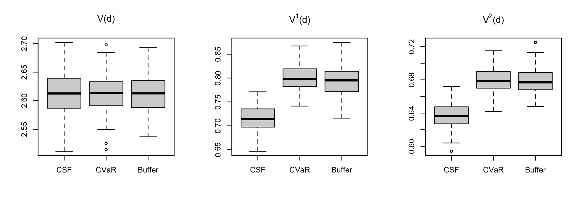
We compare our proposed methods with two baselines aimed at finding mean-optimal treatment rules: causal survival forests (CSF) (Cui et al., 2023) and CSF-based outcome-weighted learning (CSF-O) (Zhao et al., 2012), as well as approaches tailored to other decision criteria, including quantile (QuL) (Wang et al., 2018) and expected quantile (EQuL) (Xiao et al., 2019). Figure 2 summarizes the empirical values of $V(d)$, $V^{1}(d)$, and $V^{2}(d)$ across methods and scenarios. As expected, CSF and CSF-O perform competitively for the mean criterion $V(d)$. In contrast, our CVaR-based procedure consistently achieves the largest $V^{1}(d)$, and our method for the buffered criterion attains the best performance for $V^{2}(d)$.

Figure 2: Boxplots of empirical value functions.

Additional discussions of interpretability, sensitivity analyses, and further simulation results are provided in the supplementary material.

6 Real data application

We consider a randomized, double-blind, placebo-controlled trial AIDS Clinical Trials Group Protocol 175 (ACTG175) (Hammer et al., 1996) with survival time as a primary outcome. The original study designs four treatment groups with patients randomly allocated: one group receives 200 mg of zidovudine three times daily, one group is provided with 200 mg of zidovudine three times each day plus 0.75 mg of zalcitabine, one group is given 200 mg of zidovudine three times daily plus 200 mg of didanosine twice a day, while the remaining group is assigned 200 mg of didanosine twice daily.

Following Cui et al. (2023), we focus on 1083 patients receiving treatment ZDV+ddI (522 subjects) and ddI monotherapy (561 subjects). The censoring percentage is around 21%. The selected seven discrete baseline covariates include gender (904 male and 179 female), homosexual activity (725 yes and 358 no), race (772 white and 311 non-white), symptomatic status (192 symptomatic and 891 asymptomatic), history of intravenous drug use (142 yes and 941 no), hemophilia (92 yes and 991 no), and antiretroviral history (632 experienced and 451 naive). The selected five continuous baseline covariates are age, weight, Karnofsky score (scale of 0-100), CD4 count and CD8 count.

Clinically, both patients at high risk of early failure and those with good long-term prognosis are of interest in HIV studies. Early mortality is strongly associated with uncontrolled viral replication, severe immunosuppression, and opportunistic infections, so treatment rules that reduce cases of very short survival are especially valuable. At the same time, modern antiretroviral therapy has transformed HIV into a chronic condition, and long-term survival and treatment durability have become key outcomes. It is therefore desirable to assess treatment rules not only by overall mean survival but also by how they behave in clinically important tails of the survival distribution, capturing both protection against early failure and support for sustained long-term survival. In addition, the empirical survival time distribution in ACTG175 exhibits a non-negligible fraction of early failures, which further motivates a tail-sensitive analysis.

Motivated by this, we consider both methods that primarily aim to maximize mean survival time, such as CSF and CSF-O, and our methods designed to optimize the CVaR and buffered criteria. For the choice of $(\gamma,\tau)$, we adopt $\gamma\in\{0.25,0.50\},\tau\in\{460,920\}.$ For the CVaR criterion, we choose $\gamma=0.25$ and $0.50$ to focus on roughly the worst-performing patients. For the buffered criterion, we take $\tau=460$ days, which is close to the first quartile of the survival times among subjects with $\Delta=1$, so that the criterion indirectly reflects the performance of a rule with respect to early failure. The choice $\tau=920$ days (approximately 2.5 years) probes a more ambitious long-term prognosis target while still lying in a range where enough events are observed to allow reasonably stable estimation.

We use repeated $5$-fold cross-validation to evaluate each learned rule. In each replication, the data are randomly partitioned into five folds; four folds are used to train each method and the remaining fold is used for evaluation. This is repeated over all five test folds, and the entire procedure is in turn repeated $50$ times. For a generic treatment rule $d$, we denote the resulting cross-validated estimators by

$$\widetilde{V}(d) =\mathbb{P}_{\text{rep}}\left\{\mathbb{P}_{\text{test}}\left[\frac{I\{A=d(X)\}}{\widehat{\pi}(A\mid X)}\frac{\Delta Y}{\widehat{S}_{C}(Y\mid X,A)}\right]\right\},$$

$$\widetilde{V}^{1}_{\gamma}(d) =\mathbb{P}_{\text{rep}}\left\{\mathbb{P}_{\text{test}}\left[\frac{I\{A=d(X)\}}{\widehat{\pi}(A\mid X)}\left\{\widehat{\alpha}_{\gamma}\,\gamma-\frac{\Delta\big(\widehat{\alpha}_{\gamma}-Y\big)I\{\widehat{\alpha}_{\gamma}>Y\}}{\widehat{S}_{C}(Y\mid X,A)}\right\}\right]\right\},$$

$$\widetilde{M}^{2}_{\tau}(d) =\mathbb{P}_{\text{rep}}\left\{\mathbb{P}_{\text{test}}\left[\frac{I\{A=d(X)\}}{\widehat{\pi}(A\mid X)}\frac{\Delta\,\max\big\{0,\widehat{c}_{\tau}(-Y+\tau)+1\big\}}{\widehat{S}_{C}(Y\mid X,A)}\right]\right\},$$

where $\mathbb{P}_{\text{test}}$ denotes the empirical mean over the test fold, $\mathbb{P}_{\text{rep}}$ denotes the empirical mean over all repetitions. For each split, the nuisance components $\widehat{S}_{C}(\cdot|X,A)$ and $\widehat{\pi}(\cdot|X)$, as well as $(\widehat{\alpha}_{\gamma},\widehat{c}_{\tau})$, are fit using only the corresponding training folds, and the nuisance components are then evaluated on the test fold when computing $\widetilde{V}(d)$, $\widetilde{V}^{1}_{\gamma}(d)$, and $\widetilde{M}^{2}_{\tau}(d)$. Since we only have offline data from the study, these $\widetilde{V}(d)$, $\widetilde{V}^{1}_{\gamma}(d)$ and $\widetilde{M}^{2}_{\tau}(d)$ provide attainable estimators of the corresponding value functions. In particular, $\widetilde{V}(d)$ is the usual estimator of mean survival under $d$, while $\widetilde{V}^{1}_{\gamma}(d)$ and $\widetilde{M}^{2}_{\tau}(d)$ approximate the identification results introduced in Section 2.4, evaluated at the chosen $(\gamma,\tau)$ grid. It is noteworthy that larger values of $\widetilde{V}(d)$ and $\widetilde{V}^{1}_{\gamma}(d)$ and smaller values of $\widetilde{M}^{2}_{\tau}(d)$ are preferred.

Table 1 reports the cross-validated mean value $\widetilde{V}(d)$ together with the CVaR criteria ($\widetilde{V}^{1}_{0.25}(d)$ and $\widetilde{V}^{1}_{0.50}(d)$) and the buffered criteria ($\widetilde{M}^{2}_{460}(d)$ and $\widetilde{M}^{2}_{920}(d)$) for each rule. The CVaR criterion-oriented rules achieve the largest values of $\widetilde{V}^{1}_{0.25}(d)$ and $\widetilde{V}^{1}_{0.50}(d)$, indicating that, among patients in the lower tail of the survival distribution, they provide stronger protection. The buffered criterion-oriented rules exhibit lower $\widetilde{M}^{2}_{\tau}(d)$ values compared to those of the benchmarks. Taken together, these results suggest that our proposed framework can meaningfully reshape treatment allocation in a tail-sensitive direction while possibly preserving most of the gains in average survival.

Method	$\widetilde{V}(d)$	$\widetilde{V}^{1}_{0.25}(d)$	$\widetilde{V}^{1}_{0.50}(d)$	$\widetilde{M}^{2}_{460}(d)$	$\widetilde{M}^{2}_{920}(d)$
CSF	634.30	293.51	414.14	0.283	0.823
CSF-O	635.90	303.54	420.45	0.293	0.835
CVaR ($\gamma=0.25$)	632.40	305.98	421.67	0.291	0.826
CVaR ($\gamma=0.50$)	632.93	305.86	422.59	0.291	0.825
Buffered ($\tau=460$)	631.75	298.80	415.67	0.272	0.823
Buffered ($\tau=920$)	631.17	304.43	418.76	0.285	0.814

Table 1: Numerical results for the ACTG175.

7 Discussion

In this paper, we propose a novel framework to estimate the optimal treatment rules in order to control the tail of the subjects’ survival time with right-censored data. The proposed methods target directly the truncated mean survival time and survival probabilities, which are of great interest in survival analysis. For the first criterion, we maximize the truncated mean survival time by choosing a user-specified quantile endpoint; for the second criterion, we maximize survival function at a quality adjusted survival time, where the quality adjusted survival time is defined by the first value function. Moreover, the proposed methods have intrinsic connections to CVaR and bPOE, thus the resulting optimal rules can potentially prevent adverse events.

The proposed methods admit several extensions. First, as discussed in the supplementary material, a multi-arm trial can be accommodated without changing the identification arguments; for estimation, we discuss an angle-based multicategory representation and a smooth logistic relaxation, while noting that constructing a multicategory DC surrogate is substantially more challenging (Qiao and Liu, 2009; Sun et al., 2017; Zhou et al., 2018; Qi et al., 2019b; Xue et al., 2022; Zhou et al., 2023). Second, personalized dose finding with explicit tail control is a natural direction (Chen et al., 2016; Zhou et al., 2021; Fang et al., 2023). Third, extending our criteria to multi-stage (e.g., mobile health) decision-making process will require longitudinal weighting to handle time-varying treatment assignment and censoring, and will introduce additional non-smooth structure that complicates scalable optimization (Zhao et al., 2015a; Shi et al., 2018; Luckett et al., 2019; Shi et al., 2022; Ye et al., 2024; Zhou et al., 2024). Finally, it would be valuable to develop augmented inverse probability weighted, doubly robust estimators for our proposed value functions (Robins et al., 1994; Zhang et al., 2012b; Zhao et al., 2015b; Liu et al., 2018).

References

- Athey et al. (2019) Athey, S., Tibshirani, J., and Wager, S. (2019), “Generalized random forests,” The Annals of Statistics, 47, 1148–1178.
- Athey and Wager (2021) Athey, S. and Wager, S. (2021), “Policy learning with observational data,” Econometrica, 89, 133–161.
- Bickel and Lehmann (1975) Bickel, P. and Lehmann, E. (1975), “Descriptive statistics for nonparametric models II. Location,” The Annals of Statistics, 1045–1069.
- Chakraborty and Moodie (2013) Chakraborty, B. and Moodie, E. E. M. (2013), Statistical methods for dynamic treatment regimes, New York, NY: Springer.
- Chen et al. (2016) Chen, G., Zeng, D., and Kosorok, M. R. (2016), “Personalized Dose Finding Using Outcome Weighted Learning,” Journal of the American Statistical Association, 111, 1509–1521, pMID: 28255189.
- Clarke et al. (2000) Clarke, B. R., Gamble, D. K., and Bednarski, T. (2000), “A note on robustness of the beta-trimmed mean,” Australian & New Zealand journal of statistics, 42, 113–119.
- Cox (1972) Cox, D. R. (1972), “Regression models and life-tables,” Journal of the Royal Statistical Society: Series B (Methodological), 34, 187–202.
- Cui (2021) Cui, Y. (2021), “Individualized decision-making under partial identification: three perspectives, two optimality results, and one paradox,” Harvard Data Science Review, 3(3), 1–19.
- Cui and Han (2025) Cui, Y. and Han, S. (2025), “Policy learning with distributional welfare,” Journal of the American Statistical Association, 1–12.
- Cui et al. (2023) Cui, Y., Kosorok, M. R., Sverdrup, E., Wager, S., and Zhu, R. (2023), “Estimating heterogeneous treatment effects with right-censored data via causal survival forests,” Journal of the Royal Statistical Society: Series B.
- Cui et al. (2022) Cui, Y., Zhu, R., Zhou, M., and Kosorok, M. R. (2022), “Consistency of survival tree and forest models: splitting bias and correction,” Statistica Sinica, 32, 1245–1267.
- Díaz et al. (2018) Díaz, I., Savenkov, O., and Ballman, K. (2018), “Targeted learning ensembles for optimal individualized treatment rules with time-to-event outcomes,” Biometrika, 105, 723–738.
- Fang et al. (2023) Fang, E. X., Wang, Z., and Wang, L. (2023), “Fairness-oriented learning for optimal individualized treatment rules,” Journal of the American Statistical Association, 118, 1733–1746.
- Fleming and Harrington (2011) Fleming, T. R. and Harrington, D. P. (2011), Counting processes and survival analysis, vol. 169, John Wiley & Sons.
- Gelber et al. (1989) Gelber, R. D., Gelman, R. S., and Goldhirsch, A. (1989), “A quality-of-life-oriented endpoint for comparing therapies,” Biometrics, 781–795.
- Hammer et al. (1996) Hammer, S. M., Katzenstein, D. A., Hughes, M. D., Gundacker, H., Schooley, R. T., Haubrich, R. H., Henry, W. K., Lederman, M. M., Phair, J. P., Niu, M., et al. (1996), “A trial comparing nucleoside monotherapy with combination therapy in HIV-infected adults with CD4 cell counts from 200 to 500 per cubic millimeter,” New England Journal of Medicine, 335, 1081–1090.
- Hong et al. (2011) Hong, L. J., Yang, Y., and Zhang, L. (2011), “Sequential convex approximations to joint chance constrained programs: a Monte Carlo approach,” Operations Research, 59, 617–630.
- Ishwaran et al. (2008) Ishwaran, H., Kogalur, U. B., Blackstone, E. H., and Lauer, M. S. (2008), “Random survival forests,” The Annals of Applied Statistics, 2, 841 – 860.
- Jiang et al. (2017) Jiang, R., Lu, W., Song, R., and Davidian, M. (2017), “On estimation of optimal treatment regimes for maximizing t-year survival probability,” Journal of the Royal Statistical Society Series B: Statistical Methodology, 79, 1165–1185.
- Kitagawa and Tetenov (2018) Kitagawa, T. and Tetenov, A. (2018), “Who should be treated? empirical welfare maximization methods for treatment choice,” Econometrica, 86, 591–616.
- Kosorok and Laber (2019) Kosorok, M. R. and Laber, E. B. (2019), “Precision medicine,” Annual Review of Statistics and its Application, 6, 263.
- Le Thi et al. (2019) Le Thi, H. A., Van Ngai, H., and Tao, P. D. (2019), “Stochastic difference-of-convex algorithms for solving nonconvex optimization problems,” arXiv preprint arXiv:1911.04334.
- Liu and Pang (2023) Liu, J. and Pang, J.-S. (2023), “Risk-based robust statistical learning by stochastic difference-of-convex value-function optimization,” Operations Research, 71, 397–414.
- Liu and Kennedy (2021) Liu, L. and Kennedy, E. H. (2021), “Median optimal treatment regimes,” arXiv preprint arXiv:2103.01802.
- Liu et al. (2018) Liu, Y., Wang, Y., Kosorok, M. R., Zhao, Y., and Zeng, D. (2018), “Augmented outcome-weighted learning for estimating optimal dynamic treatment regimens,” Statistics in Medicine, 37, 3776–3788.
- Luckett et al. (2019) Luckett, D. J., Laber, E. B., Kahkoska, A. R., Maahs, D. M., Mayer-Davis, E., and Kosorok, M. R. (2019), “Estimating dynamic treatment regimes in mobile health using V-learning,” Journal of the American Statistical Association, 0, 1–34.
- Lugosi and Mendelson (2021) Lugosi, G. and Mendelson, S. (2021), “Robust multivariate mean estimation: The optimality of trimmed mean,” Annals of Statistics, 49, 393–410.
- Mafusalov and Uryasev (2018) Mafusalov, A. and Uryasev, S. (2018), “Buffered probability of exceedance: mathematical properties and optimization,” SIAM Journal on Optimization, 28, 1077–1103.
- Norton and Uryasev (2019) Norton, M. and Uryasev, S. (2019), “Maximization of auc and buffered auc in binary classification,” Mathematical Programming, 174, 575–612.
- Pang et al. (2016) Pang, J.-S., Razaviyayn, M., and Alvarado, A. (2016), “Computing B-stationary points of nonsmooth DC programs,” Mathematics of Operations Research, 42, 95–118.
- Qi et al. (2019a) Qi, Z., Cui, Y., Liu, Y., and Pang, J.-S. (2019a), “Estimation of individualized decision rules based on an optimized covariate-dependent equivalent of random outcomes,” SIAM Journal on Optimization, 29, 2337–2362.
- Qi et al. (2019b) Qi, Z., Liu, D., Fu, H., and Liu, Y. (2019b), “Multi-armed angle-based direct learning for estimating optimal individualized treatment rules with various outcomes,” Journal of the American Statistical Association, 1–33.
- Qi et al. (2023) Qi, Z., Pang, J.-S., and Liu, Y. (2023), “On robustness of individualized decision rules,” Journal of the American Statistical Association, 118, 2143–2157.
- Qian and Murphy (2011) Qian, M. and Murphy, S. A. (2011), “Performance guarantees for individualized treatment rules,” Annals of statistics, 39, 1180.
- Qiao and Liu (2009) Qiao, X. and Liu, Y. (2009), “Adaptive weighted learning for unbalanced multicategory classification,” Biometrics, 65, 159–168.
- Robins et al. (1994) Robins, J. M., Rotnitzky, A., and Zhao, L. P. (1994), “Estimation of regression coefficients when some regressors are not always observed,” Journal of the American statistical Association, 89, 846–866.
- Rockafellar and Royset (2010) Rockafellar, R. T. and Royset, J. O. (2010), “On buffered failure probability in design and optimization of structures,” Reliability Engineering & System Safety, 95, 499–510.
- Rockafellar and Uryasev (2000) Rockafellar, R. T. and Uryasev, S. (2000), “Optimization of conditional value-at-risk,” Journal of Risk, 2, 21–42.
- Rockafellar and Uryasev (2020) — (2020), “Minimizing buffered probability of exceedance by progressive hedging,” Mathematical Programming, 181, 453–472.
- Rosenbaum and Rubin (1983) Rosenbaum, P. R. and Rubin, D. B. (1983), “The Central Role of the Propensity Score in Observational Studies for Causal Effects,” Biometrika, 70, 41–55.
- Shi et al. (2018) Shi, C., Fan, A., Song, R., and Lu, W. (2018), “High-dimensional A-learning for optimal dynamic treatment regimes,” Annals of Statistics, 46, 925.
- Shi et al. (2022) Shi, C., Zhang, S., Lu, W., and Song, R. (2022), “Statistical inference of the value function for reinforcement learning in infinite-horizon settings,” Journal of the Royal Statistical Society Series B: Statistical Methodology, 84, 765–793.
- Steinwart and Christmann (2008) Steinwart, I. and Christmann, A. (2008), Support vector machines, Springer Science & Business Media.
- Stensrud et al. (2024) Stensrud, M. J., Laurendeau, J., and Sarvet, A. L. (2024), “Optimal regimes for algorithm-assisted human decision-making,” Biometrika, 111, 1089–1108.
- Sun et al. (2017) Sun, H., Craig, B. A., and Zhang, L. (2017), “Angle-based Multicategory Distance-weighted SVM,” Journal of Machine Learning Research, 18, 1–21.
- Sun et al. (2019) Sun, Q., Zhu, R., Wang, T., and Zeng, D. (2019), “Counting process-based dimension reduction methods for censored outcomes,” Biometrika, 106, 181–196.
- Tian et al. (2014) Tian, L., Zhao, L., and Wei, L. (2014), “Predicting the restricted mean event time with the subject’s baseline covariates in survival analysis,” Biostatistics, 15, 222–233.
- Tsiatis et al. (2019) Tsiatis, A. A., Davidian, M., Holloway, S. T., and Laber, E. B. (2019), Dynamic treatment regimes: Statistical methods for precision medicine, Chapman and Hall/CRC.
- Uno et al. (2014) Uno, H., Claggett, B., Tian, L., Inoue, E., Gallo, P., Miyata, T., Schrag, D., Takeuchi, M., Uyama, Y., Zhao, L., et al. (2014), “Moving beyond the hazard ratio in quantifying the between-group difference in survival analysis,” Journal of Clinical Oncology, 32, 2380.
- Wang et al. (2018) Wang, L., Zhou, Y., Song, R., and Sherwood, B. (2018), “Quantile-optimal treatment regimes,” Journal of the American Statistical Association, 113, 1243–1254.
- Xiao et al. (2019) Xiao, W., Zhang, H. H., and Lu, W. (2019), “Robust regression for optimal individualized treatment rules,” Statistics in Medicine, 38, 2059–2073.
- Xue et al. (2022) Xue, F., Zhang, Y., Zhou, W., Fu, H., and Qu, A. (2022), “Multicategory Angle-Based Learning for Estimating Optimal Dynamic Treatment Regimes With Censored Data,” Journal of the American Statistical Association, 117, 1438–1451.
- Ye et al. (2024) Ye, H., Zhou, W., Zhu, R., and Qu, A. (2024), “Stage-aware learning for dynamic treatments,” Journal of Machine Learning Research, 25, 1–51.
- Zhang et al. (2012a) Zhang, B., Tsiatis, A. A., Davidian, M., Zhang, M., and Laber, E. (2012a), “Estimating optimal treatment regimes from a classification perspective,” Stat, 1, 103–114.
- Zhang et al. (2012b) Zhang, B., Tsiatis, A. A., Laber, E. B., and Davidian, M. (2012b), “A robust method for estimating optimal treatment regimes,” Biometrics, 68, 1010–1018.
- Zhao et al. (2025) Zhao, P., Josse, J., and Yang, S. (2025), “Efficient and robust transfer learning of optimal individualized treatment regimes with right-censored survival data,” Journal of Machine Learning Research, 26, 1–54.
- Zhao et al. (2012) Zhao, Y., Zeng, D., Rush, A. J., and Kosorok, M. R. (2012), “Estimating individualized treatment rules using outcome weighted learning,” Journal of the American Statistical Association, 107, 1106–1118.
- Zhao et al. (2015a) Zhao, Y.-Q., Zeng, D., Laber, E. B., and Kosorok, M. R. (2015a), “New statistical learning methods for estimating optimal dynamic treatment regimes,” Journal of the American Statistical Association, 110, 583–598.
- Zhao et al. (2015b) Zhao, Y.-Q., Zeng, D., Laber, E. B., Song, R., Yuan, M., and Kosorok, M. R. (2015b), “Doubly robust learning for estimating individualized treatment with censored data,” Biometrika, 102, 151.
- Zhou et al. (2024) Zhou, W., Zhu, R., and Qu, A. (2024), “Estimating optimal infinite horizon dynamic treatment regimes via pt-learning,” Journal of the American Statistical Association, 119, 625–638.
- Zhou et al. (2021) Zhou, W., Zhu, R., and Zeng, D. (2021), “A parsimonious personalized dose-finding model via dimension reduction,” Biometrika, 108, 643–659.
- Zhou et al. (2017) Zhou, X., Mayer-Hamblett, N., Khan, U., and Kosorok, M. R. (2017), “Residual weighted learning for estimating individualized treatment rules,” Journal of the American Statistical Association, 112, 169–187.
- Zhou et al. (2018) Zhou, X., Wang, Y., and Zeng, D. (2018), “Outcome-weighted learning for personalized medicine with multiple treatment options,” 2018 IEEE 5th International Conference on Data Science and Advanced Analytics (DSAA), 565–574.
- Zhou et al. (2023) Zhou, Z., Athey, S., and Wager, S. (2023), “Offline multi-action policy learning: generalization and optimization,” Operations Research, 71, 148–183.