Efficient Graph Coloring with Neural Networks: A Physics-Inspired Approach for Large Graphs

Abstract

Combinatorial optimization problems near algorithmic phase transitions represent a fundamental challenge for both classical algorithms and machine learning approaches. Among them, graph coloring stands as a prototypical constraint satisfaction problem exhibiting sharp dynamical and satisfiability thresholds. Here we introduce a physics-inspired neural framework that learns to solve large-scale graph coloring instances by combining graph neural networks with statistical-mechanics principles. Our approach integrates a planting-based supervised signal, symmetry-breaking regularization, and iterative noise-annealed neural dynamics to navigate clustered solution landscapes. When the number of iterations scales quadratically with graph size, the learned solver reaches algorithmic thresholds close to the theoretical dynamical transition in random graphs and achieves near-optimal detection performance in the planted inference regime. The model generalizes from small training graphs to instances orders of magnitude larger, demonstrating that neural architectures can learn scalable algorithmic strategies that remain effective in hard connectivity regions. These results establish a general paradigm for learning neural solvers that operate near fundamental phase boundaries in combinatorial optimization and inference.

Keywords Graph coloring $\cdot$ Physics-inspired Machine Learning $\cdot$ Graph neural networks $\cdot$ Graph coloring $\cdot$ Statistical Physics $\cdot$ Optimization Problem $\cdot$ Potts model

1 Introduction

The graph coloring problem (GCP) is a paradigmatic constrained optimization problem that lies at the core of combinatorial complexity theory. It consists of assigning one among $q$ possible colors to each vertex of an undirected graph, so that no two adjacent vertices share the same color. The problem of deciding whether a graph can be fairly colored with $q$ colors is NP-complete Karp (2010), while the optimization of a graph’s coloring to minimize conflicts is NP-hard Garey and Johnson (1979). Beyond its theoretical relevance, graph coloring arises in a wide range of practical applications, including scheduling Lewis (2021), timetabling Ahmed (2012) and even puzzle solving such as Sudoku Tosuni (2015), moreover it can be reduced in polynomial time to all other NP-hard problems Karp (2010) as the travelling salesman problem, the clique problem or k-SAT Garey and Johnson (1979). The intrinsic difficulty of the GCP is deeply connected to the widely held belief that $P\neq NP$ Garey and Johnson (1979) Fortnow (2009), making the GCP both difficult and useful to solve. In large random graphs, the structure of the solution space undergoes sharp phase transitions as the average connectivity varies. These transitions dramatically affect the performance of algorithms, creating regimes in which solutions exist but are algorithmically hard to find. Understanding and overcoming these barriers remains a central challenge in combinatorial optimization. Classical approaches to graph coloring typically rely on local search in configuration space Galinier and Hertz (2006). Monte Carlo Markov Chain (MCMC) methods such as Simulated Annealing Chams et al. (1987) Johnson et al. (1991) Angelini and Ricci-Tersenghi (2023), TabuCol Hertz and Werra (1987), and evolutionary algorithms Galinier and Hao (1999); Malaguti et al. (2008); Mostafaie et al. (2020), can achieve strong performance, but may require running times that grow exponentially with graph size in hard regimes. Greedy heuristics such as Greedy coloring Matula and Beck (1983) or DSatur Brélaz (1979), avoid the problem of time scaling but provide sub-optimal solutions. In recent years, graph neural networks (GNNs) have emerged as a promising alternative paradigm, leveraging relational inductive biases to process graph-structured data. Several works have applied GNNs to graph coloring, using reinforcement learning, direct classification of colorability, or physics-inspired energy minimization strategies. While these approaches demonstrate encouraging results, their performance often degrades near critical connectivity thresholds, precisely where the problem becomes structurally hardest.

In this work, we introduce a physics-inspired neural framework that explicitly integrates statistical-mechanics insights into the training and inference dynamics of a GNN-based solver. Our approach combines three key ingredients: (i) a planting procedure that provides supervised guidance while preserving statistical properties of random graph ensembles in relevant regimes; (ii) a semi-supervised loss that blends a differentiable Potts energy with symmetry-breaking overlap terms; and (iii) an iterative noise-annealed inference procedure that enables the model to escape metastable configurations in clustered solution landscapes. By scaling the number of inference iterations with the problem size, we demonstrate that the learned solver approaches the dynamical phase transition threshold in random graphs and achieves near-optimal detection performance in the planted inference regime. Moreover, the model generalizes from training on relatively small graphs to solving instances orders of magnitude larger, highlighting the potential of neural architectures to learn scalable algorithmic strategies rather than memorizing instance-specific patterns.

This paper is structured as follows. In section 2, we provide a high-level overview of existing methods based on GNNs. In Sec. 3 we address the GCP from a statistical mechanics point of view, highlighting its connections with the Potts model. We describe the two types of graphs used in this work, namely Erdős–Rényi and planted graphs, describing the procedure for generating them. In Sec. 4 we detail the dataset used in this work, we present a novel GNN-based architecture and introduce an effective supervised training strategy, and we describe the coloring procedure. In Sec. 5 we presents the performances of our method in terms of energy and scaling at different connectivities, comparing it to simulated annealing. We show how our method is preferable to simulated annealing in a wide region of connectivities and number of nodes, in terms of speed, scalability and final energy.

2 Related Work

There is a vast and diverse list of algorithms used to solve NP-hard problems. In this section, we focus on algorithms that primarily use Graph Neural Networks (GNNs) for solving the GCP.

In Huang et al. (2019), improved heuristics for graph coloring are sought using reinforcement learning, leveraging a deep neural network architecture that has access to the entire graph structure. In Lemos et al. (2019), a GNN is used to determine whether a graph can be colored using $q$ colors or not. Additionally, it is shown how node embeddings can be used to assign coloring to the graph. In Li et al. (2022), the performances of aggregation-combine GNNs are studied. The work highlights the features that limit the expressive power of these models in solving node-classification problems under strong heterophily (including the GCP) and proposes solutions to improve performances.

In Schuetz et al. (2022), the authors use the architecture of a physics-inspired GNN (PI-GNN) for graph coloring. Specifically, the neural network is optimized in order to minimize the Potts energy of the given graph. This approach has been adopted in several subsequent works. In Wang et al. (2023), an alternative to PI-GNN is proposed, introducing negative-message-passing, achieving numerical improvements. Additionally, an entropic term is introduced in the loss function to accelerate convergence during the model training. Finally, in Zhang et al. (2024), a graph isomorphism network model, using a physics-inspired approach, is proposed. The output of the neural network, is post-processed using TabuCol to reduce the number of conflicts.

3 Background

In this section, we formally introduce the graph coloring problem and its connection to the Potts model, furthermore the graphs ensembles used in this work are presented and the algorithm used to generate them is described.

3.1 Graph coloring

The GCP is a very well-known constraint satisfaction problem (CSP) easily understandable yet difficult to solve. Formally, we consider an undirected graph ${\mathcal{G}=(\mathcal{V},\mathcal{E})}$ where ${\mathcal{V}=\{1,...,N\}}$ is the set of vertices and ${\mathcal{E}=\{(i,j)|i,j\in\mathcal{V}\}}$ is the set of edges. The objective is to assign an integer variable (or color) ${s_{\nu}\in\{1,...,q\}}$ to each node $\nu\in\mathcal{V}$, such that nodes sharing the same edge have different colors, namely

$$s_{i}\neq s_{j},\ \forall(i,j)\in\mathcal{E}$$ (1)

If a graph admits such a configuration $\mathbf{s}$, the graph is said $q$-colorable. The smallest value of $q$ for which the graph is colorable is the chromatic number $\chi(\mathcal{G})$ of the graph.

3.2 Potts model

Figure 1: Phase transitions in the graph coloring problem from Zdeborová and Krzakala (2007).

Searching for configurations of nodes that satisfy graph coloring is equivalent to studying the energy minima of the anti-ferromagnetic Potts model Wu (1982). The Potts model is the generalization of an Ising model, where the spins can take $q$ different values. The Hamiltonian of the model is given by

$$H_{\text{Potts}}(\mathbf{s})=-\sum_{(i,j)\in\mathcal{E}}J_{ij}\delta_{s_{i},s_{j}}\;.$$ (2)

It is easy to verify that the energy value in the anti-ferromagnetic case ($J_{ij}=-1\ \ \forall(i,j)\in\mathcal{E}$), corresponds to the number of conflicting edges in the associated GCP. In the thermodynamic limit the nodes configurations $\mathbf{s}$ for a given graph $\mathcal{G}$ in equilibrium at temperature $T$ follows the Gibbs-Boltzmann probability distribution

$$P_{\mathcal{G}}(\mathbf{s})=\frac{e^{-\beta H(\mathbf{s})}}{\mathcal{Z}}\;,$$ (3)

where $\beta=\frac{1}{K_{B}T}$, $K_{B}$ is the Boltzmann constant and we have defined the partition function

$$\mathcal{Z}=\sum_{\{\mathbf{s}\}}e^{-\beta H(\mathbf{s})}\;.$$ (4)

In the limit $\beta\to\infty$, the measure is dominated by the minimum energy configurations. Therefore, the measure is the uniform distribution over the configurations that satisfy

$$E_{0}=\min_{\mathbf{s}}H(\mathbf{s})\;.$$ (5)

If $E_{0}=0$, the graph is $q$-colorable and if an algorithm is able to sample from the $\beta\rightarrow{\infty}$ distribution, then it is able to solve the GCP Mezard and Montanari (2009). This principle is behind the working of some graph coloring algorithms as simulated annealing Kirkpatrick et al. (1983) and belief propagation Pearl (2022).

It is well known that the solution space of GCP for random graphs such as Random Regular Graphs (RRG) Bollobás and Bollobás (1998) and Erdős–Rényi Graphs (ERG) Erdös and Rényi (1959) undergoes multiple phase transitions Zdeborová and Krzakala (2007). In Fig. 1 we report a visual representation of the solution space in each phase. The success of sampling and the time required to perform it strongly depend on the average connectivity of the graph under consideration and the number of colors $q$. In particular, for sufficiently small connectivity values $c<c_{d}(q)$, all solutions to the problem (or at least the vast majority of them) form a single connected cluster, and it is possible to go from one solution to another solution by modifying a sub-extensive number of node variables. Additionally, in this phase, finding solutions is particularly easy regardless of the algorithm used. In the $q>3$ case, at $c_{d}(q)$ a dynamic phase transition takes place, such that for $c>c_{d}(q)$ the solutions are shattered among exponentially many (in $N$) clusters; this structure of solutions generally slows down the dynamics of algorithms looking for solutions to the GCP. In the range $c_{c}(q)<c<c_{s}(q)$, the number of clusters of zero-energy states becomes sub-exponential. In this region, despite the existence of solutions, finding them using algorithms that scale polynomially with problem size is particularly challenging. Finally, in the region with high connectivity values, that is beyond the satisfiability threshold, $c>c_{s}(q)$, the probability that a random graph is $q$-colorable vanishes in the large $N$ limit. We stress that the above scenario holds only in the thermodynamic limit, while for finite-size graphs, there are corrections to this behavior, e.g., it is still possible to have a $q$-colorable random graph with $c>c_{s}$. The $q\leq 3$ case is less significant, as the $c_{d}(q)$ and $c_{c}(q)$ critical thresholds coincide, resulting in a situation that is generally easier to tackle for algorithms.

4 Methods

In this section, we describe the model architecture and dataset. The loss function and training method are then introduced. Finally, the algorithm used for searching the solution is presented and motivated.

4.1 Model

We are interested in learning a map $f(\cdot;\mathcal{G})$ from a feature space $\mathcal{X}\in\mathbb{R}^{k\times N}$ to a color space $\{1,\dddot{},q\}^{N}$ such that:

$$H_{\text{Potts}}\big[f(\{\mathbf{x}_{i}\}_{i\in\mathcal{V}};\mathcal{G})\big]=0$$ (6)

We choose to parameterize this map with a GNN model, implementing the transformation $f_{\boldsymbol{\theta}}(\cdot;\mathcal{G})$. GNNs are designed to leverage the invariance properties of graph structures, making them effective for learning representations that respect the underlying graph topology.

In recent years, a plethora of architectures have been presented in the context of GNNs Zhou et al. (2021). For our purposes, we have focused on one of the most general and expressive models, described in Battaglia et al. (2018), and already used with promising results in solving various tasks Tang et al. (2023); Wieder et al. (2020); Wang et al. (2019). The model used in this work is based on a message passing network composed by $L$ layers. At each layer nodes features are updated as follows: at first for each edge an ingoing and an outgoing message are computed, (each node sends and receives a message from its neighbors) using the formula

$$\textbf{m}_{ij}^{(l)}=\phi^{(l)}_{\theta_{1}^{(l)}}\left(\mathbf{x}_{i}^{(l-1)},\mathbf{x}_{j}^{(l-1)}\right)\;,$$ (7)

where $\textbf{m}_{ij}^{(l)}$ represents the message sent by the $j^{\text{th}}$ node and gathered by the $i^{\text{th}}$ node in the $l^{\text{th}}$ layer, while $\mathbf{x}_{i}^{(l-1)}$ and $\mathbf{x}_{j}^{(l-1)}$ represent the node features at the previous layer. Next, the messages are aggregated using any permutation invariant function (e.g. sum, average, max). Together with the node features from the previous step $\mathbf{x}_{i}^{(l-1)}$, the aggregated messages are used to update the node features:

$$\mathbf{x}_{i}^{(l)}=\gamma^{(l)}_{\theta_{2}^{(l)}}\left(\mathbf{x}_{i}^{(l-1)},\bigoplus_{j\in\mathcal{N}(i)}\textbf{m}_{ij}^{(l)}\right)\;,$$ (8)

where $\mathcal{N}(i)$ is the set of neighbors of node $i$ in the graph. The functions $\phi^{(l)}_{\theta_{1}^{(l)}}$ and $\gamma^{(l)}_{\theta_{2}^{(l)}}$, used to compute the messages and the node features respectively, are parameterized by two multi layer perceptrons (MLP). After the $L^{\text{th}}$ layer, all hidden and input features are passed to a third MLP $\Gamma_{\theta_{3}}$ to compute the final output of the node:

$$\mathbf{x}_{i}^{\text{output}}=\text{softmax}\Big[\Gamma_{\theta_{3}}(\{\mathbf{x}^{(l)}_{i}\}_{l=0,\dots,L})\Big]$$ (9)

The softmax activation makes the output feature vector normalized. In this way the $a^{\text{th}}$ component of $\mathbf{x}_{i}^{\text{output}}$ can be interpreted as a node’s probability of having the $a^{\text{th}}$ color. We denote the overall function implemented by the parametric model with $f_{\boldsymbol{\theta}}\big(\{\mathbf{x}_{i}^{(0)}\}_{i\in\mathcal{V}}\big)$, where $\boldsymbol{\theta}$ represents the set of all trainable parameters and we denote the input feature vector associated to the $i^{\text{th}}$ node with $\mathbf{x}_{i}^{(0)}$. We highlight that by construction, the hidden features $\mathbf{x}_{i}^{(l)}$ contain information about all neighbors at distance $l$ from the $i^{\text{th}}$ node. Moreover the output function $\Gamma_{\theta_{3}}$ is able to use all intermediate features at once, effectively learning to process messages gathered at different graph distances.

4.2 Dataset

We are interested in training our algorithm using both supervised and unsupervised loss terms. To do so, we need a dataset of graphs satisfying the GCP. It is already well known that finding a good strategy to train neural networks to solve problems for which it is hard to have a solution is a challenging point. In this paper we overcome this problem, using the efficient planting procedure to obtain a random graph together with a solution of the GCP that could be however hard to find even for very smart algorithms Krzakala and Zdeborová (2009). The ensemble of graphs generated with this planting procedure is usually referred to as the planted ensemble and, in some region of the parameters, is contiguous to the random Erdős–Rényi ensemble of graphs.

4.2.1 Erdős–Rényi random graphs

An Erdős–Rényi graph $\mathcal{G}(N,M)$ is a type of random graph generated by selecting exactly $M$ edges uniformly at random from the set of all possible $\binom{N}{2}$ edges. The number of edges is connected to the graph average connectivity $c$ and number of nodes $N$ through the formula

$$M=\frac{c\,N}{2}\;.$$ (10)

The space of solution of the GCP on this ensemble of graphs undergoes the transition pictorially represented in Fig. 1.

4.2.2 Planted Erdős–Rényi random graphs

As we have discussed in Secs. 1 and 3.2, finding a perfect coloring for a generic graph can be very resource-expensive. To this end, in the present paragraph, we briefly discuss a simple and effective method that allows us to generate graphs for which a solution $\mathbf{s}^{*}$ is already known Krzakala and Zdeborová (2009). The procedure is explained in algorithm 1.

Algorithm 1 Planting algorithm

1:Input: Number of nodes $N$, number of colors $q$, number of edges $M=\frac{cN}{2}$

2:Assign each node $i\in\mathcal{V}$ a color $s_{i}\in\{1,\dots,q\}$ such that each color appears $\sim\frac{N}{q}$ times

3:Initialize an empty edge set $|\mathcal{E}|=0$

4:while $|\mathcal{E}|<M$ do

5:  Sample nodes $i,j\in\mathcal{V}$ uniformly at random

6:  if $s_{i}\neq s_{j}$ and $(i,j)\notin\mathcal{E}$ then

7:   Add edge $(i,j)$ to $\mathcal{E}$

8:  else

9:   Sample new nodes $i,j\in\mathcal{V}$ uniformly at random

10:  end if

11:end while

Notably, this algorithm can generate fairly colored graphs at any connectivity, even beyond the satisfiability threshold ($c>c_{s}$). It can be proved that planted random graphs are indistinguishable from random graphs as long as $c<c_{c}$ Krzakala and Zdeborová (2009). For this reason, in that region, the procedure is called quiet-planting. When $c>c_{c}$, the entropy of the planted state (i.e., the set of solutions around the planted one) becomes larger than the entropy of all other random solutions, making the planted random graph distinguishable from a standard (non-planted) random graph. However, the model that we introduce in Sec. 4 does not aim to sample graphs from the Gibbs distribution, but to find a solution that minimizes the energy. Therefore, the solutions obtained by the planting procedure continue to be suitable for the purpose of training.

In the planted model, the planted solution can be detected only if the value of $c$ is large enough. At present, the best detection algorithm is Belief Propagation, which is successful for $c>c_{\text{KS}}$, where $c_{\text{KS}}$ is the Kesten-Stigum bound, whose role in inference problems has been discussed in detailed in the literature Krzakala and Zdeborová (2009); Ricci-Tersenghi et al. (2019).

4.3 Training and loss function

In this work, we are interested in training a model that, given a colored graph with conflicting edges, produces a perfect coloring. Hence we are interested in finding a map

$$f:\{1,\dddot{},q\}^{N}\longrightarrow\{1,\dddot{},q\}^{N}$$ (11)

To this end, the model has been trained with a semi-supervised loss function, including an energy term and a term which measures the closeness of the output with the perfectly colored solution. The training is performed using a gradient-descent-based algorithm, therefore the loss function must be differentiable with respect to the model’s parameters. This is not possible by using the Potts energy directly, as it is not differentiable. For this reason, regarding the energy term in the loss function, we have employed a continuous version of the Potts energy, introduced in Schuetz et al. (2022):

$$H_{\text{Potts}}^{c}\big[\{\mathbf{y}_{i}\}_{i\in\mathcal{V}}\big]=\sum_{(i,j)\in\mathcal{E}}\langle\textbf{y}_{i},\mathbf{y}_{j}\rangle\;,$$ (12)

where the $a^{\text{th}}$ component of $\mathbf{y}_{i}$, indicated as $y_{i}^{a}$, is the probability of the $a^{\text{th}}$ color to be assigned to the $i^{\text{th}}$ node. For this reason, both spaces described in Eq. (11) are extended to $\mathbb{R}^{q\times N}$.

Regarding the supervised term in the loss function, this is inspired by a denoising autoencoder Vincent et al. (2008), which forces the model to map corrupted inputs by adding noise (thus moving them away from the solution clusters) into inputs belonging to the solution manifold. In our case, the model is trained by taking a planted solution $\{\boldsymbol{\xi}_{i}\}_{i\in\mathcal{V}}$, written in the extended space, to which noise $\{\boldsymbol{\epsilon}_{i}\}_{i\in\mathcal{V}}\sim\mathcal{N}(\boldsymbol{0},\hat{I})$ is added

$$\{\tilde{\mathbf{x}}_{i}\}_{i\in\mathcal{V}}=\sqrt{\alpha}\{\boldsymbol{\xi}_{i}\}_{i\in\mathcal{V}}+\sqrt{1-\alpha}\{\boldsymbol{\epsilon}_{i}\}_{i\in\mathcal{V}}$$ (13)

and including in the loss function a term which measures the closeness of the input planted graph to the output of the model.

A third contribution to the loss is given by an entropy term, measuring the average output node entropy. This term is used only during the initial steps of training to help the algorithm escape the region of parameter space that corresponds to the paramagnetic state $\Big(\big[f_{\boldsymbol{\theta}}(\{\textbf{x}_{i}\}_{i\in\mathcal{V}})\big]_{j}^{a}=\frac{1}{q},\forall j\in\mathcal{V},\forall a\in\{1,\dddot{},q\}\Big)$. We have empirically observed that this term does not lead to a final lower energy but increases the convergence speed. The final loss function is then given by

$$L(\{\textbf{x}_{i}\}_{i\in\mathcal{V}},\{\boldsymbol{\xi}_{i}\}_{i\in\mathcal{V}};\boldsymbol{\theta})=\\ \mathbb{E}_{\{\boldsymbol{x}_{i}\}_{i\in\mathcal{V}}}\big[h\left[f_{\boldsymbol{\theta}}(\{\textbf{x}_{i}\}_{i\in\mathcal{V}})\right]\big]\\ +\eta_{1}\,\mathbb{E}_{\{\boldsymbol{x}_{i}\}_{i\in\mathcal{V}}}\big[S\left[f_{\boldsymbol{\theta}}(\{\textbf{x}_{i}\}_{i\in\mathcal{V}})\right]\big]\\ -\eta_{2}\,\mathbb{E}_{\{\boldsymbol{x}_{i}\}_{i\in\mathcal{V}}}\big[O\left[f_{\boldsymbol{\theta}}(\{\textbf{x}_{i}\}_{i\in\mathcal{V}}),\{\boldsymbol{\xi}_{i}\}_{i\in\mathcal{V}}\right]\big]$$

where $\eta_{1}$ and $\eta_{2}$ are relative weights and the three contributions are respectively an energy term, namely the percentage of conflicting edges, the features entropy and the overlap with the planted solution. These terms are given by

$$h\left[f_{\boldsymbol{\theta}}(\{\textbf{x}_{i}\}_{i\in\mathcal{V}})\right]=\frac{1}{M}\sum_{(i,j)\in\mathcal{E}}\langle f_{\boldsymbol{\theta}}(\{\boldsymbol{x}\})_{i},f_{\boldsymbol{\theta}}(\{\boldsymbol{x}\})_{j}\rangle$$

$$S\left[f_{\boldsymbol{\theta}}(\{\textbf{x}_{i}\}_{i\in\mathcal{V}})\right]=-\sum_{i\in\mathcal{V}}f_{\boldsymbol{\theta}}(\{\boldsymbol{x}\})_{i}\cdot\log_{2}f_{\boldsymbol{\theta}}(\{\boldsymbol{x}\})_{i}$$

$$O\left[f_{\boldsymbol{\theta}}(\{\textbf{x}_{i}\}_{i\in\mathcal{V}}),\boldsymbol{\xi}_{i}\right]=\frac{1}{|\mathcal{V}|}\sum_{i\in\mathcal{V}}\langle f_{\boldsymbol{\theta}}(\{\boldsymbol{x}\})_{i},\boldsymbol{\xi}_{i}\rangle$$

where $A_{ij}$ is the adjacency matrix and

$$h\left[\{\textbf{x}_{i}\}_{i\in\mathcal{V}}\right]=\frac{1}{M}H_{\text{Potts}}^{c}\big[\{\mathbf{x}_{i}\}_{i\in\mathcal{V}}\big]$$ (14)

The overlap term is necessary to break the permutation symmetry of the colors. In fact, the energy and entropy terms in the loss are invariant for color permutations. Consequently the loss landscape contains $q!$ identical regions, each corresponding to equivalent, permuted colorings. Breaking this symmetry simplifies the map that the model needs to learn, as the loss landscape is modified so that only the planted solution has the lowest loss, guiding the optimizer more efficiently.

The training phase of our model is detailed in algorithm 2. Both $\alpha_{\text{min}}$ and $\alpha_{\text{max}}$ are hyperparameters of the algorithm, which have led to the best results when set respectively to 0.4 and 0.9.

Algorithm 2 Training algorithm (batch size = $1$)

1:for $n=1,\ldots,N_{\text{epochs}}$ do

2:  Sample: $\alpha\sim\text{Uniform}(\alpha_{\text{min}},\alpha_{\text{max}})$

3:  Sample planted coloring: $\{\boldsymbol{\xi}_{i}\}_{i\in\mathcal{V}}$

4:  Sample noise: $\{\boldsymbol{\epsilon}_{i}\}_{i\in\mathcal{V}}\sim\mathcal{N}(\boldsymbol{0},\hat{I})$

5:  Compute:

6:     $\{\tilde{\mathbf{x}}_{i}\}_{i\in\mathcal{V}}=\sqrt{\alpha}\{\boldsymbol{\xi}_{i}\}_{i\in\mathcal{V}}+\sqrt{1-\alpha}\{\boldsymbol{\epsilon}_{i}\}_{i\in\mathcal{V}}$

7:  Forward pass through GNN:

8:     $\{\mathbf{x}_{i}\}_{i\in\mathcal{V}}=f_{\boldsymbol{\theta}}(\{\tilde{\mathbf{x}}_{i}\}_{i\in\mathcal{V}})$

9:  Compute loss: $L(\{\textbf{x}_{i}\}_{i\in\mathcal{V}},\{\boldsymbol{\xi}_{i}\}_{i\in\mathcal{V}};\boldsymbol{\theta})$

10:  Backpropagate to compute:

11:      $\nabla_{\boldsymbol{\theta}}L(\{\textbf{x}_{i}\}_{i\in\mathcal{V}},\{\boldsymbol{\xi}_{i}\}_{i\in\mathcal{V}};\boldsymbol{\theta})$

12:  Update parameters

13:end for

4.4 Coloring

In this paragraph, we detail the coloring process using our trained model $f_{\boldsymbol{\theta}}\big(\cdot\big)$. For a sufficiently expressive model, we would expect to find the perfect coloring with a single forward pass ($N_{\text{iter}}=1$). For our model, however, we have empirically observed that this is not the case, as the output energy is further reduced with subsequent applications of the same trained model. We call $N_{\text{iter}}$ the number of iterations, that is, subsequent applications of the model. Additionally, we have observed that the algorithm used is characterized by fixed points that do not correspond to the solutions of the GCP. This causes the algorithm to get stuck in sub-optimal configurations. We have verified that performances are greatly improved by adding noise after each forward step, as described in Eq. 13. We experimented with different choices for noise scheduling. The best performances were achieved with linearly increasing values of $\alpha$ between $\alpha_{\text{min}}=0.25$ and $\alpha_{\text{max}}=0.9$. During this noise-annealing procedure, the neural network gradually reduces the energy of the input graph. If it is performed for a large enough number of iterations, this procedure eventually leads the graph into the attraction basin of a zero-energy solution. The scheduling of noise from large to smaller values has the meaning of letting the model explore a larger portion of the color space in the initial steps, while making the model collapse towards the zero-energy solution in the final steps. We have empirically observed how this procedure produces very similar results even when a solution is not guaranteed to exist. A more detailed discussion on how noise modifies the forward step is discussed in App. A. A detailed description of the coloring procedure is given in algorithm 3.

Algorithm 3 Graph coloring algorithm

1:Initialize random coloring: $\{\mathbf{x}^{(0)}_{i}\}_{i\in\mathcal{V}}$

2:Set: $\alpha_{\text{arr}}=\text{Linspace}(\alpha_{\text{min}},\alpha_{\text{max}},T)$

3:for $t=0,\ldots,N_{\text{iter}}-1$ do

4:  Sample Gaussian noise: $\{\boldsymbol{\epsilon}_{i}\}_{i\in\mathcal{V}}\sim\mathcal{N}(\boldsymbol{0},\hat{I})$

5:  Compute:

6:    $\{\tilde{\mathbf{x}}^{(t)}_{i}\}=\sqrt{\alpha_{\text{arr}}[t]}\{\mathbf{x}^{(t)}_{i}\}+\sqrt{1-\alpha_{\text{arr}}[t]}\{\boldsymbol{\epsilon}_{i}\}$

7:  Forward step:

8:     $\{\mathbf{x}^{(t+1)}_{i}\}_{i\in\mathcal{V}}=f_{\boldsymbol{\theta}}(\{\tilde{\mathbf{x}}_{i}^{(t)}\}_{i\in\mathcal{V}})$

9:

10:  if $\mathbf{x}^{(t+1)}$ is a solution then

11:   Return $\mathbf{x}^{(t+1)}$

12:  end if

13:end for

5 Experiments

In this section, we show the performances of our algorithm in coloring both random graphs and planted graphs with $q=5$ colors. In order to study both the generalization capabilities and its behaviour around the phase transitions, we report results in three main configurations: Model A is trained on a wide range of connectivities and a fixed number of nodes, to assess the generalisation capabilities to larger graphs; Model B and Model C are trained and tested on two restricted connectivity regions around the phase transitions, to evaluate the algorithm behaviour at the critical points.

5.1 Models setup

In the following, we provide the details of the training dataset and the architecture for each of the three models.

In Model A, we have used 5 layers and a latent space dimension of 32. The number of parameters of each MLP in the model is reported in Table 1. To train Model A, we have used a dataset of $1000$ planted graphs for each connectivity in $[12.5,12.6,12.7,\dddot{},14.9,15]$, for a total of 26k graphs. Each graph in the dataset has $N=1000$ nodes. We have used $90\%$ of the dataset to train the model and $10\%$ for validation. We have tested Model A on independently generated samples with a larger number of nodes.

Component	Structure		Parameters
$\phi_{\theta_{1}^{(1)}}$	layer 1	$2673$	$2673$
	layers 2–5	$4\times 4455$	$17{,}820$
$\gamma_{\theta_{2}^{(1)}}$	layer 1	$3564$	$3564$
	layers 2–5	$4\times 4455$	$17{,}820$
$\Gamma_{\theta_{3}}$	output	—	$6968$
Total			48,845

Table 1: Trainable parameters for Model A.

In Model B, we have used 10 layers and a latent space dimension of 64. The number of parameters of each MLP in the model is reported in Table 2. To train Model B, we have used a dataset of $4000$ planted graphs for each connectivity in $[12.5,12.7,12.9,\dddot{},13.5,13.7]$, and sizes $N=[1024,2048,4096]$ for a total of 84k graphs. This dataset has been proposed as a hard benchmark to test neural-network-based solvers Skenderi et al. (2026). We have used $90\%$ of the dataset to train the model and $10\%$ for validation. We have tested Model B on independently generated samples with an equal or larger number of nodes.

Component	Structure		Parameters
$\phi_{\theta_{1}^{(1)}}$	layer 1	$9425$	$9425$
	layers 2–10	$9\times 17095$	$153{,}855$
$\gamma_{\theta_{2}^{(1)}}$	layer 1	$13520$	$13520$
	layers 2–10	$9\times 17095$	$153{,}855$
$\Gamma_{\theta_{3}}$	output	—	$47{,}325$
Total			377,980

Table 2: Trainable parameters for Model B and C.

In Model C, we have used 10 layers and a latent space dimension of 64. The number of parameters of each MLP in the model is reported in Table 2. To train Model C, we have used a dataset of $10000$ planted graphs for each connectivity in $[16.5,17.0,17.5]$, and size $N=10000$ for a total of 30k graphs. We have used $90\%$ of the dataset to train our model and $10\%$ for validation. We have tested Model C on independently generated samples with an equal or larger number of nodes.

In all models, we have used $q=5$ colors and an additional input feature to encode the node’s degree. We have observed that this additional feature increases the model performance with a negligible computational cost. We trained the models for 2000 epochs (Model A) or 1500 epochs (Model B and Model C) using a batch size of $64$, $\eta_{1}=0.5$, and $\eta_{2}=0.05$, setting $\eta_{1}$ to zero after the first epoch. We have used the Adam optimizer Kingma and Ba (2014) for parameter optimization.

5.2 Results

In this section, we report the results obtained for each of the three models introduced above, showing the scaling properties of the models and comparing them to state-of-the-art algorithms.

To facilitate the interpretation of the results, we summarize the critical values for $q=5$: $c_{d}=12.837(3)$, $c_{c}=13.23(1)$ and $c_{s}=13.669(2)$ for 5-coloring of random graphs Zdeborová and Krzakala (2007), while $c_{\text{KS}}=16$ for detection of the planted configuration Krzakala and Zdeborová (2009).

Figure 2: (Model A) Extensive energy as a function of the number of iterations for four representative connectivity values, $c=11.5,13.0,13.5,15.5$. Each data point is obtained by averaging results over 50 graphs with $N=$10k nodes. Circles indicate values for planted graphs, while crosses indicate values for random graphs.

Model A Fig. 2 shows the scaling with the number of iterations of the extensive energy $E$, which counts the number of unsatisfied edges. We plot data for 4 connectivities, corresponding to the 4 main phases of the solution space, separated by the critical values $c_{d}$, $c_{c}$, and $c_{s}$. As shown in Fig. 2, the scaling behaviour of the mean energy—which is similar for random and planted models in this range of connectivities—exhibits a clear dependence on the connectivity parameter $c$. For $c=11.5$, the energy decays faster than a power-law, indicating an efficient exploration of the energy landscape in the sparse regime. At $c=13.0$, the decay is approximately consistent with a power-law, suggesting a transition point where the algorithm still maintains an effective scaling with the number of iterations. It is worth stressing that for $c=13.0$ we are in a clustered phase, where other algorithms (e.g., equilibrium Monte Carlo samplings) would face serious limitations in converging to problem solutions. In contrast, for $c=13.5$ and $c=15.5$, the energy decreases significantly more slowly than a power-law, reflecting a pronounced slowdown in convergence.

Figure 3: (Model A) Main panel Mean intensive energy as a function of connectivity, for both random and plante graphs, and a number of nodes varying from $N=3$k to $N=100$k. Each data point is obtained by running the algorithm for $N_{\text{iter}}=200$k iterations and averaging the energy over 50 graphs. Inset The mean extensive energy grows with the size at each value of $c$ and does not allow to determine the algorithmic threshold in the large $N$ limit.

The main panel of Fig. 3 shows the intensive energy $e=E/N$ as a function of the connectivity. It is worth noticing that data are very similar, for both random and planted graphs, in the whole range of sizes $3000\leq N\leq 10^{5}$. Thus, we assume to have reached the large $N$ limit, and we can make the claim that the mean energy $e$ becomes non-zero close to the dynamical critical point $c_{d}$, and Model A is not able to find solutions for larger values of $c$.

In the inset of Fig. 3, we report the same data for the mean extensive energy $E$ on a logarithmic scale to make evident that, even in the region where $e$ looks very small, the number of violated constraints $E$ is actually growing with the graph size $N$. Under these conditions, it is not possible to get any meaningful estimate for the algorithmic threshold $c_{\text{alg}}$. Indeed, for $c_{\text{alg}}$, in the large $N$ limit, the algorithm should be able to find a solution with high probability, and this implies that the mean extensive energy $E$ should go to zero.

The observation that an algorithmic threshold can not be estimated from the data shown in Fig. 3 suggests that the number of iterations should not be kept constant, but scaled with the problem size $N$ to properly identify $c_{\text{alg}}$. This has already been observed in the behaviour of other algorithms, like simulated annealing Angelini et al. (2025), solving the same graph coloring problem. The improved scaling of the number of iterations with the problem size will be used in Model B and Model C.

Model B To better estimate the algorithmic threshold $c_{\text{alg}}$ of the model, we trained and tested a new and more expressive architecture on a narrow connectivity region, centered around the phase transition $c_{d}$. This choice allows us to test the model behaviour precisely where the problem complexity is expected to increase sharply.

Figure 4: (Model B) Probability of finding a solution as a function of the graph connectivity $c$, for sizes $N\in[1024,2048,4096,8192]$ and a number of iterations scaling as $N_{\text{iter}}=0.04\,N^{2}$. Each point is the average over 400 graphs.

Figure 5: (Model B) Comparison of the probability of finding a solution as a function of the graph connectivity $c$ for different solving algorithms. Values are obtained by averaging over $400$ graphs of $N=1024$ nodes. The number of iterations $N_{\text{iter}}$ is chosen to ensure the same wall-clock execution time across all algorithms. The tested algorithms are a recurrent Physics-Inspired GNN (rPI) Schuetz et al. (2022), Belief Propagation (BP) Skenderi et al. (2026), Simulated Annealing (SA) Angelini et al. (2025), our graph neural network (GNN), and Focused Metropolis Search (FMS) Seitz et al. (2005).

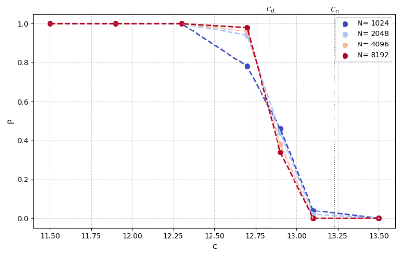
In Fig. 4 we plot the probability of finding a solution using Model B run for a number of iterations scaling quadratically with the graph size, $N_{\text{iter}}=0.04\,N^{2}$. The curves become sharper as the problem size $N$ increases and cross very close to $c_{d}$ (marked with a vertical dashed line). Thus we conclude that our solver based on a GNN run for a number of iterations scaling quadratically with the problem size has an algorithmic threshold very close to the dynamical transition, $c_{\text{alg}}\simeq c_{d}$.

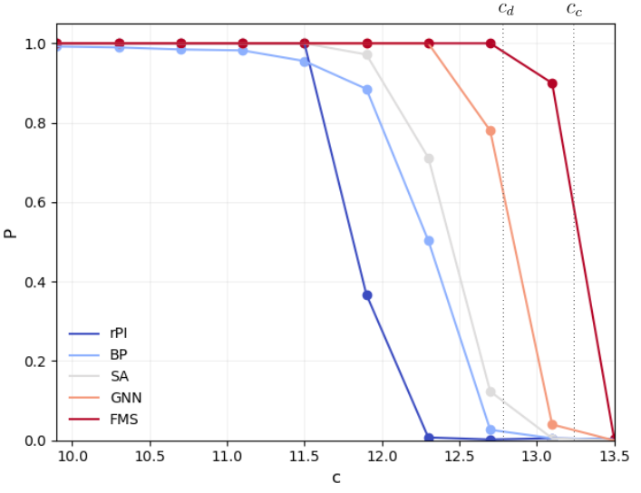
Whether this value for the algorithmic threshold is good or not with respect to other solvers can be understood by looking at the curves plotted in Fig. 5, which represent the probability of finding a solution in random graphs of size $N=1024$ by several different smart algorithms. We stress that we are considering the algorithms which are known to be the best available at present to solve the random graph coloring problem. These algorithms have been already compared in recent studies Angelini et al. (2025); Skenderi et al. (2026). We notice that our GNN-based algorithm is performing very well, ranking second just after Focused Metropolis Search (FMS), which is known to have impressive performances in this class of hard optimization problems Angelini et al. (2025). Reaching performances which are better than those of algorithms considered highly competitive in the field (Simulated Annealing, Belief Propagation, the Physics-Inspired GNN introduced in Ref. Schuetz et al. (2022)) is a major achievement of our algorithm.

Model C While for $c<c_{c}$ random graphs and planted graphs have the same statistical properties, for $c>c_{c}$ the planted configuration can be detected in principle. In this regime, coloring of planted graphs is a prototypical hard inference problem, where the signal to be detected is the planted coloring, and the graph connectivity $c$ plays the role of the signal-to-noise ratio. Indeed, the more the edges (compatible with the planted coloring by construction), the more information to detect the planted configuration.

Bayes optimal algorithms (like Belief Propagation Krzakala and Zdeborová (2009)) can detect the planted coloring with $q=5$ colors when $c>c_{\text{KS}}=16$, and this is considered the best achievable in polynomial time. Indeed, most of the spectral algorithms show poorer performances Krzakala et al. (2013). Recently, the behavior of Simulated Annealing (SA) to solve this inference problem has been explored in detail: the standard version of SA has a larger algorithmic threshold ($c_{\text{KS}}^{\text{SA}}\simeq 18$), but an improved version with multiple interacting copies, replicated SA (rSA), shows optimal performances ($c_{\text{KS}}^{\text{rSA}}\simeq 16$).

Figure 6: (Model C) Main panel Probability of finding a solution as a function of the graph connectivity $c$, for sizes $2500\leq N\leq 20000$ and a number of iterations scaling as $N_{\text{iter}}=10^{-4}\,N^{2}$. Each point is the average over $2\,10^{6}/N$ graphs. Inset The mean overlap with the planted coloring of the configuration output by the algorithm.

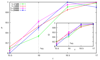
In the main panel of Fig. 6 we plot the probability of finding a proper coloring of the graph as a function of the connectivity $c$, when the algorithm is run for a number of iteration growing quadratically with the problem size, $N_{\text{iter}}=10^{-4}\,N^{2}$. For the range of graphs we have explored, $2500\leq N\leq 20000$, the curves show a weak size dependence and they sharply increase around the optimal threshold $c_{\text{KS}}=16$. Moreover the inset show the mean overlap with the planted coloring, and the similarity with the data presented in the main panel confirm that the solution found is (or is very close to) the planted one. Thus, we have proven that our algorithm solves the inference problem of detecting the planted configuration in a close to optimal way. This is once more an impressive result, making our GNN-based solver competitive with the state-of-the-art algorithms.

6 Conclusions

We have introduced an algorithm that leverages physics-inspired graph neural networks to solve efficiently the planted graph coloring problem, which provides hard instances of both optimization and inference problems depending on the random graph connectivity. Our algorithm clearly outperforms any machine-learning–based method previously available (see the recent comparative study in Ref. Skenderi et al. (2026)) and it is competitive with other known algorithms: it ranks second, beyond Focused Metropolis Search (an impressive local search algorithm) in the optimization problem, and it reaches the optimal algorithmic threshold in the inference problem.

A key conceptual contribution of this work is the integration of statistical-mechanics principles into the learning process. Impressive performances have been achieved implementing a novel approach that uses planted solutions to introduce supervised signals without sacrificing the statistical structure of hard random ensembles, while symmetry breaking and noise-annealed iteration enable controlled navigation of clustered energy landscapes, avoiding the common problem of over-smoothing in GNNs. It is also very important to stress that the optimal performances reported in the present work have been possible only thanks to the scaling of the number of iterations with the problem size. In particular, inspired by a recent work Angelini et al. (2025), we have chosen a scaling where the number of iterations grows quadratically with the problem size.

Our results strongly suggest that further research in this direction is not only promising but necessary in order to push the current limits of machine learning methods used in high-dimensional combinatorial optimization and inference. Our study shows that, for certain connectivity regimes, the performance of the algorithm does not significantly vary across different graph sizes. The ability of the trained model to generalize from relatively small graphs to instances orders of magnitude larger highlights another important perspective. Instead of learning instance-specific mappings, the network appears to internalize structural regularities of the problem class. This suggests a route toward foundation models for algorithmic reasoning on graphs—models that are trained on synthetic ensembles capturing the essential structural properties of a problem family and then deployed across scales and instances.

The results presented in this work extend beyond the specific case of graph coloring and contribute to a broader research direction: the development of neural solvers that operate effectively near algorithmic phase transitions. Many hard combinatorial optimization and inference problems—including SAT, Max-Cut, community detection, error-correcting codes, and resource allocation exhibit sharp structural transitions separating easy and algorithmically challenging regimes. These transitions often coincide with fragmentation of the solution space into exponentially many clusters, where traditional search heuristics become trapped in metastable states. Our findings suggest that neural architectures, when trained with appropriate structural guidance and iterative dynamics, can learn strategies that remain effective precisely in these critical regions.

From an applied standpoint, scalable neural solvers for large combinatorial instances could impact domains such as communication networks, distributed computing, logistics, circuit design, and scheduling, where large-scale graph-structured constraints are ubiquitous. At the same time, improvements in solving hard CSPs may influence cryptographic constructions and complexity-based hardness assumptions, underscoring the importance of continued theoretical scrutiny.

Several open directions emerge from this study. First, a deeper theoretical understanding of why quadratic iteration scaling enables threshold-optimal behavior remains to be developed. Second, extending this framework to heterogeneous graph ensembles, weighted constraints, or real-world network topologies would test its robustness beyond random models. Third, integrating learned neural dynamics with classical message-passing or local-search algorithms could yield adaptive hybrid solvers that combine interpretability with learned flexibility.

Ultimately, this work contributes to a growing perspective in machine learning: that learning can complement complexity theory and statistical physics in exploring the algorithmic limits of hard problems. By explicitly targeting phase boundaries and structural bottlenecks, neural solvers may help bridge the gap between theoretical optimality and practical scalability in combinatorial optimization and inference.

Appendix A Effects of noise during coloring

(a) Comparison at connectivity 11.5
·

(b) Comparison at connectivity 13.0

(c) Comparison at connectivity 13.5

(d) Comparison at connectivity 15.5

Figure 7: Fractions of conflicting edges (intensive energy) as a function of the iteration step during a coloring loop for different connectivities. Data for coloring with (without) noise are represented in red (blue). Two standard deviations are reported with the shaded area.

As discussed in the main text, one the key observations is that a single application of our trained model does not solve, in general, the graph coloring problem. As detailed in Sec. 4.4, we have observed that only by repeatedly applying the same map $f_{\boldsymbol{\theta}}(\cdot,\mathcal{G})$ (trained model) to the input state, the energy decreases, reaching a set of configurations, forming a basin of attraction composed of energy-stable (or stationary) configurations $\mathbf{x}^{\text{ES}}$, defined by the equation:

$$h\big[f_{\boldsymbol{\theta}}(\{\mathbf{x}^{\text{ES}}_{i}\}_{i\in\mathcal{V}})\big]\approx h\big[\{\mathbf{x}^{\text{ES}}_{i}\}_{i\in\mathcal{V}}\big]\;.$$ (15)

These attractor states rarely correspond to zero-energy configurations (i.e., solutions), unless the coloring process is repeated for a large enough number of iterations $N_{\text{iter}}$.

Moreover, we empirically observed a performance improvement when corrupting the algorithm input with noise before every new step, namely when using

$$\mathbf{x}^{(t+1)}_{i}=f_{\boldsymbol{\theta}}(\sqrt{\alpha}\,\mathbf{x}^{(t)}_{i}+\sqrt{1-\alpha}\,\boldsymbol{\epsilon},\mathcal{G})\,,$$ (16)

where $\boldsymbol{\epsilon}\sim\mathcal{N}(\mathbf{0},\hat{I})$ we observe a higher probability of converging to solutions.

In Fig. 7, the two coloring procedures—with and without noise—are compared for different values of connectivity. From the figure, it is evident that adding noise during the coloring loop greatly decreases the final energy reached by our algorithm.

Here, we aim to provide a possible explanation for this behavior. Let us consider zero-energy solutions $\boldsymbol{\xi}$ and energy-stable configurations $\mathbf{x}^{\text{ES}}$, as defined above. We are interested in showing what happens when we apply our trained model to these solutions, after they are corrupted with noise. Namely, we look at

$$\begin{cases}\tilde{\boldsymbol{\xi}}_{i}(\alpha)=f_{\boldsymbol{\theta}}(\sqrt{\alpha}\,\boldsymbol{\xi}_{i}+\sqrt{1-\alpha}\,\boldsymbol{\epsilon},\mathcal{G})\\ \tilde{\mathbf{x}}^{\text{ES}}_{i}(\alpha)=f_{\boldsymbol{\theta}}(\sqrt{\alpha}\,\mathbf{x}^{\text{ES}}_{i}+\sqrt{1-\alpha}\,\boldsymbol{\epsilon},\mathcal{G})\end{cases}$$ (17)

where $\boldsymbol{\epsilon}\sim\mathcal{N}(\mathbf{0},\hat{I})$. We are interested in measuring the fraction of conflicts (intensive energy) in the output configuration when the input configuration is corrupted by noise and comparing it with the same quantity in the energy-stable configurations or zero-energy solutions. In formulae we compute $\Delta h_{\alpha}(\mathbf{z})=h[\tilde{\mathbf{z}}(\alpha)]-h[\mathbf{z}]$, where $\mathbf{z}$ is either the energy-stable configuration $\mathbf{x}^{\text{ES}}$ or the zero-energy solution $\boldsymbol{\xi}$.

(a) $\Delta h_{\alpha}(\boldsymbol{\xi})$ for zero-energy solutions.

(b) $\Delta h_{\alpha}(\mathbf{x}^{\text{ES}})$ for energy-stable configurations.

Figure 8: Differences in intensive energies around solutions (left) or energy-stable configurations (right) obtained by perturbing the configuration according to Eq. 17. We use $N=10$k and $c=11.5,13.0,13.5,15.5$. The right panel shows that is possible to find lower energy configurations by perturbing the energy-stable states.

In Fig. 8 we report the difference in intensive energy $\Delta h_{\alpha}(\boldsymbol{\xi})$ (left panel) and $\Delta h_{\alpha}(\mathbf{x}^{\text{ES}})$ (right panel), that provide information on the energy landscape around the zero-energy solutions $\boldsymbol{\xi}$ and the energy-stable configurations $\mathbf{x}^{\text{ES}}$. Perturbing a zero-energy solution $\boldsymbol{\xi}$ we get always a larger energy (left panel), while perturbing energy-stable configurations $\mathbf{x}^{\text{ES}}$ we may obtain configurations of lower energy (right panel). This suggests that in the latter case, the noise may allow to leave basin of attractions of the energy-stable state and find lower energy configurations.

(a) Average values (lines) with one standard deviation (shaded areas) for the overlaps $O\big[\tilde{\textbf{x}}^{\text{ES}}(\alpha),\textbf{x}^{\text{ES}}\big]$ and $O\big[\tilde{\boldsymbol{\xi}}(\alpha),\boldsymbol{\xi}\big]$ as a function of $\alpha$.

(b) Average values (lines) with one standard deviation (shaded areas) for the overlaps difference $\Delta O=O\big[\tilde{\boldsymbol{\xi}}(\alpha),\boldsymbol{\xi}\big]-O\big[\tilde{\textbf{x}}^{\text{ES}}(\alpha),\textbf{x}^{\text{ES}}\big]$ as a function of $\alpha$.

Figure 9: Comparison between the overlap before and after the application of the trained model and the difference of overlaps between zero-energy solution and energy-stable configurations.

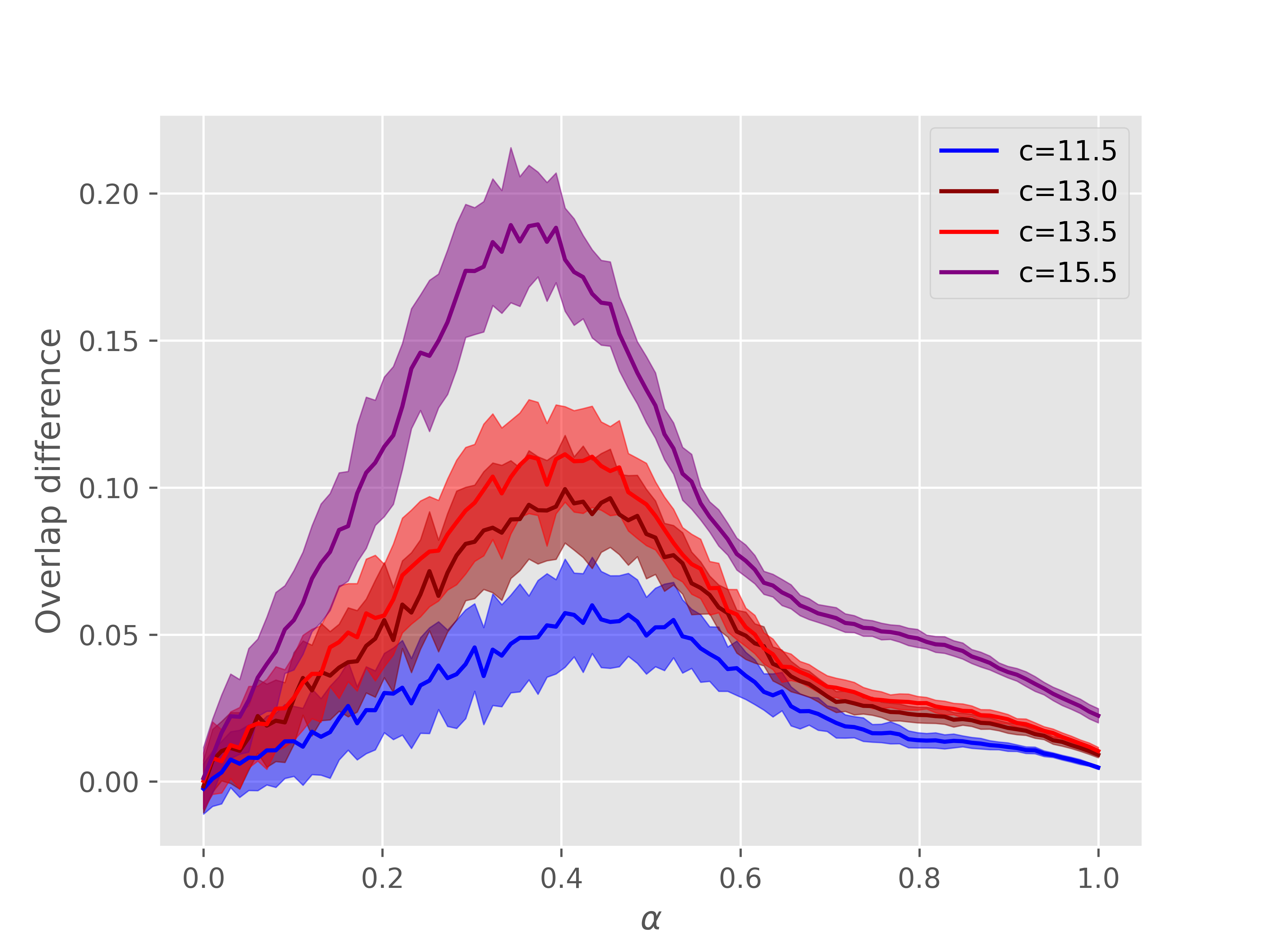
It is also interesting to study the behavior of the overlap between the original configuration (either $\boldsymbol{\xi}$ or $\mathbf{x}^{\text{ES}}$) and the corresponding processed configuration, obtained via Eq. 17. We define the overlap as follows

$$\begin{cases}O\big[\tilde{\boldsymbol{\xi}}(\alpha),\boldsymbol{\xi}\big]=\frac{1}{|\mathcal{V}|}\sum_{i\in\mathcal{V}}\langle\tilde{\boldsymbol{\xi}}_{i}(\alpha),\boldsymbol{\xi}_{i}\rangle\\ O\big[\tilde{\textbf{x}}^{\text{ES}}(\alpha),\textbf{x}^{\text{ES}}\big]=\frac{1}{|\mathcal{V}|}\sum_{i\in\mathcal{V}}\langle\tilde{\textbf{x}}^{\text{ES}}_{i}(\alpha),\textbf{x}^{\text{ES}}_{i}\rangle\end{cases}$$ (18)

We report in Fig. 9(a) the two overlaps as a function of $\alpha$ for several values of $c$ and in Fig. 9(b) their difference $\Delta O=O\big[\tilde{\boldsymbol{\xi}}(\alpha),\boldsymbol{\xi}\big]-O\big[\tilde{\textbf{x}}^{\text{ES}}(\alpha),\textbf{x}^{\text{ES}}\big]$. It is clear that the zero-energy solutions are typically more attractive (i.e., have larger overlaps).

.