Climate Transition to Temperate Nightside at High Atmosphere Mass

Abstract

Our recent work shows how M-Earth climates and transmission spectra depend on the amount of ice-free ocean on the planet’s dayside and the mass of N₂ in its atmosphere. M-Earths with more ice-free ocean and thicker atmospheres are hotter and more humid, and have larger water vapour features in their transmission spectra. In this paper, we describe a climate transition in high-pN₂ simulations from the traditional “eyeball” M-Earth climate, in which only the substellar region is temperate, to a “temperate nightside” regime in which both the dayside and the nightside are entirely ice-free. Between these two states, there is a “transition” regime with partial nightside ice cover. We use 3D climate simulations to describe the climate transition from frozen to deglaciated nightsides. We attribute this transition to increased advection and heat transport by water vapour in thicker atmospheres. We find that the nightside transitions smoothly back and forth between frozen and ice-free when the instellation or pCO₂ is perturbed, with no hysteresis. We also find an analogous transition in colder planets: those with thin atmospheres can have a dayside hotspot when the instellation is low, whereas those with more massive atmospheres are more likely to be in the “snowball” regime, featuring a completely frozen dayside, due to the increased advection of heat away from the substellar point. We show how both of these climate transitions are sensitive to instellation, land cover, and atmosphere mass. We generate synthetic transmission spectra and phase curves for the range of climates in our simulations.

1 Introduction

Recent studies have shown that M-Earths can have ice-free nightsides when the incident flux or greenhouse gas abundance is sufficient (Turbet et al., 2016; Komacek & Abbot, 2019; Zhang & Yang, 2020; Paradise et al., 2022). Our recent work (Macdonald et al., 2022, 2024a) has shown that the combined effects of unconstrained land cover and atmosphere mass result in a large range of possible M-Earth climate states, which will be difficult to differentiate in transit spectra. Following up on these results, this paper focuses on a climate transition to a new climate regime at high atmosphere mass (pN₂), featuring a fully deglaciated nightside, moist atmosphere, and small day-to-night temperature gradient. This new regime is a departure from the frozen nightside and partially deglaciated dayside typical of M-Earth climates. We also present a transition regime featuring a partially deglaciated nightside. This climate transition occurs because more massive atmospheres are conducive to increased day-night heat transport through dayside evaporation and advection of water vapour to the nightside. This paper describes these transition-related mechanisms in detail.

Although some M-Earth climates with ice-free or partly ice-covered nightsides have been identified in previous work, and the effects of atmosphere mass have been investigated in asynchronously rotating planets with Sun-like hosts, as discussed below, we are unaware of any detailed description of this climate transition on synchronously rotating planets with M-dwarf hosts to date. In this paper, we characterize the transition for M-Earths and discuss the dependence of the transition threshold on dayside land cover. We describe the physical effects of pN₂ on climate in Section 2, describe our simulations and climate regimes in Section 3, discuss climate transition mechanisms and validation tests in Section 4, present synthetic observations in Section 5, and discuss our results in Section 6.

2 Climate Effects of N₂ Partial Pressure

N₂ is not a greenhouse gas, and it is difficult to detect in transmission spectra due to a lack of strong infrared absorption features (Benneke & Seager, 2012). It can nonetheless have significant climate effects when it makes up a large proportion of the atmosphere, as it does on Earth. As a background gas, N₂ affects dynamics, heat transport, humidity, and surface temperature. N₂ has a direct radiative effect through Rayleigh scattering and an indirect radiative effect through pressure broadening of other species. These climate effects are described below.

2.1 Pressure Broadening

Pressure broadening of greenhouse gases is a warming effect: interactions with background gas molecules causes a broadening of a gas’ absorption lines, resulting in an amplification of the greenhouse effect as more radiation is absorbed by the atmosphere (Goldblatt et al., 2009). Kopparapu et al. (2014) found that in warm wet atmospheres, the pressure broadening of H₂O vapour lines warms the surface by significantly reducing outgoing longwave radiation. CO₂ lines are also broadened, resulting in an enhanced CO₂ greenhouse effect. The impact on H₂O is larger because of a positive temperature-water vapour feedback: although the saturation vapour pressure of H₂O does not depend directly on the background gas pressure, it has a strong dependence on temperature, which itself is very sensitive to pN₂. H₂O abundance is therefore highly sensitive to pN₂. More massive atmospheres are warmer and can therefore hold more water vapour, whose greenhouse effect is then amplified by pressure broadening (Keles et al., 2018).

2.2 Rayleigh Scattering

Rayleigh scattering is a cooling effect with a $\lambda^{-4}$ dependence, meaning that shortwave radiation is preferentially scattered, regardless of atmospheric composition. A higher surface pressure means that more molecules are available to scatter photons; consequently, the cooling effect increases with the partial pressure of N₂ or other gases. The cooling effect of Rayleigh scattering at high pN₂ dominates over the warming effect of pressure broadening for planets with Sun-like spectra (Keles et al., 2018; Komacek & Abbot, 2019; Paradise et al., 2021). However, since Rayleigh scattering is weaker for M-Earths due to the redder spectra of M-dwarfs (Ramirez, 2020), the warming effect of pressure broadening can be expected to continue to outweigh the cooling effect of Rayleigh scattering at high surface pressures for M-Earths.

2.3 General Circulation

There is a lapse rate warming feedback associated with increased pN₂: the moist adiabatic lapse rate increases with pressure, bringing it closer to the dry adiabatic lapse rate. On Earth, this results in decreased convection in the tropics and therefore a warmer surface (Goldblatt et al., 2009; Xiong et al., 2022). Meanwhile, the atmosphere’s total heat capacity increases with mass, leading to a decrease of high-latitude lower-troposphere radiative cooling (Chemke et al., 2016).

Zhang & Yang (2020) describe a change in the general circulation of a synchronously rotating M-Earth with increasing pN₂: the substellar upwelling region becomes larger, the downwelling region becomes smaller, and the horizontal and vertical winds become much slower. These changes result in a higher upper-troposphere relative humidity, and therefore in warming due to an enhanced water vapour greenhouse effect. They also note that despite the reduction in wind speed, the magnitude of the mass streamfunction increases with pN₂ because the atmosphere is more massive; consequently, the day-night temperature gradient is reduced because more heat is transported to the nightside. This circulation trend is analogous to the trend for Earth-like planets, on which thicker atmospheres lead to slower zonal winds, greater mass transfer, more efficient heat transport, and smaller equator-to-pole temperature gradients (Kaspi & Showman, 2015; Wordsworth, 2016).

3 Description of Simulations

3.1 Simulation Parameters

We use the 3D general circulation model (GCM) ExoPlaSim (Paradise et al., 2022). The parameters for our simulations are described in Table 1. We use the Group C simulations from Macdonald et al. (2024a) and variations on these. The 0.2 M_⊕ planet is synchronously rotating around a 2600 K star. This system is optimized for transit spectroscopy: the planet’s transit depth is largest with a small host star, and the planet’s low mass results in a large atmospheric scale height, which makes spectral features easier to detect than on an Earth-sized planet.

We vary the dayside land fraction from 0 to 100% using the Substellar Continent (SubCont) and Substellar Ocean (SubOcean) configurations described in Figure 1 of Macdonald et al. (2022). SubCont is a circular continent centred at the substellar point with ocean everywhere else. SubOcean is the opposite: a circular ocean centred at the substellar point with land everywhere else. The original Group C simulations all receive 881.7 W/m² of instellation to match Proxima Centauri b, with the orbital period and rotation rate adjusted for a 2600 K star. In this paper, we also include variations with instellations of 700, 800 and 1000 W/m², with the rotation periods adjusted accordingly and all other parameters unchanged, to explore how colder and warmer climates respond to pN₂ variations.

Parameter	Group C (Macdonald et al., 2024a)	Variations	Perturbations
Radius (R⊕)	0.646	–	–
Mass (M⊕)	0.2	–	–
Gravity (m/s2)	4.7	–	–
Period (days)	4.96	5.89, 5.33, 4.51	–
pN2 (bar)	0.5, 1, 2, 4, 6, 8	–	–
pCO2 (millibar)	1	–	0.2 – 3
Stellar temperature (K)	2600	–	–
Stellar radius (R⊙)	0.1	–	–
Stellar flux (W/m2)	881.7	700, 800, 1000	810 – 910
Resolution (lat$\times$lon)	$64\times 128$	–	$32\times 64$

Table 1: Description of simulations.

We also include some lower-resolution simulations to explore cycles between climate states, by varying either the pCO₂ or the instellation. Although the quantitative threshold for the climate transition can be resolution-dependent, the mechanism of the transition is the same at both resolutions. Our results are therefore qualitatively valid, and the more efficient configuration makes multi-millennium simulations feasible.

3.2 Climate Regimes

Our simulations generally fall into four distinct climate regimes (Figure 1). Each planet’s climate state is determined by the combined effects of land cover, instellation, pN₂, and pCO₂. These regimes are as follows:

Figure 1: Surface temperature (top row) and sea ice (bottom row) maps of aquaplanets in the snowball, eyeball, transition, and temperate nightside climate regimes.

• The “eyeball” regime (Pierrehumbert, 2011), featuring a frozen nightside and a partially deglaciated dayside, is the basic climate regime expected for M-Earths, given the distribution of incident flux on synchronously rotating planets. The simulations in Macdonald et al. (2022, 2024a) are mostly in this regime. The size of the deglaciated region depends on the instellation, pN₂, and amount of ice-free ocean on the planet’s dayside. Eyeball climates with substellar continents have drier atmospheres and larger day-night temperature contrasts than those with large substellar oceans.

• The “snowball” regime features below-freezing daysides and nightsides. This regime is found in low-instellation simulations, especially those with high pN₂.

• The “temperate nightside” regime describes models with above-freezing temperatures everywhere on the surface. This regime is found in high-instellation, high-pN₂ models.

• The “transition” regime features a deglaciated dayside and a partially deglaciated nightside. The frozen regions of the nightside are near the poles and the antistellar point; they are not radially symmetric because of the influence of atmospheric circulation patterns. This regime spans a smaller parameter space than the others.

Figure 2: Zonal mean zonal wind for aquaplanets with varying pN₂ (rows) and instellation (columns). Most have the Rhines rotator circulation pattern of two jet streams. The jets become slower with increasing pN₂ and faster with increasing flux, until the circulation breaks down at high flux and pN₂ due to the transition to the temperate nightside regime.

Figure 3: Tidally locked streamfunction (Hammond & Lewis, 2021; Paradise et al., 2022) for aquaplanets with varying pN₂ (rows) and instellation (columns). Most have the Rhines rotator circulation pattern of an overturning cell from the substellar point toward the nightside. The circulation intensifies with both increasing flux and increasing pN₂, even though the latter results in slower winds, because the amount of mass being circulated is increasing. There is a sharp transition to a much weaker streamfunction associated with the transition to the temperate nightside regime (bottom right).

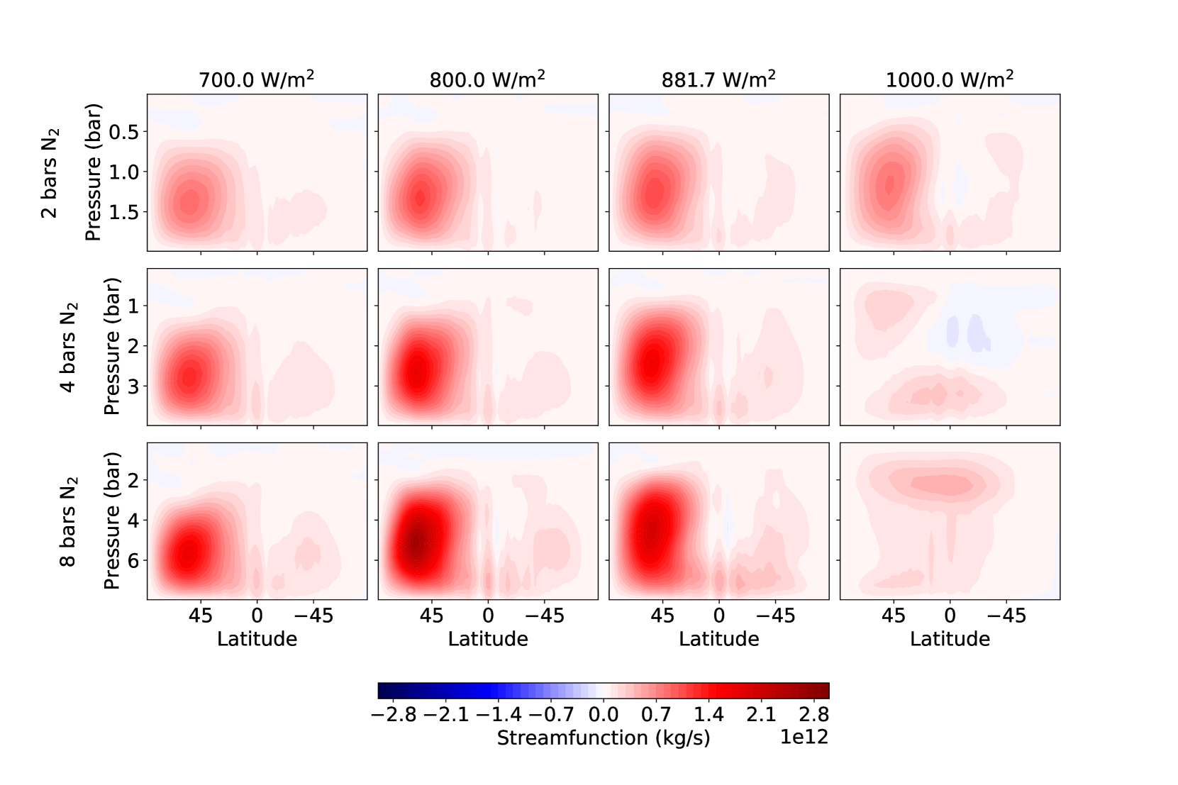
Figures 2 and 3 show the circulation patterns of aquaplanets with a range of instellations and pN₂. We obtain the trend of reduced wind speeds and increasing mass transport streamfunction magnitude pointed out by Zhang & Yang (2020). As in the case of Earth-like planets (Kaspi & Showman, 2015; Komacek & Abbot, 2019), the strength of the circulation and the zonal wind speeds mostly increase with increasing incident flux; however, we find that the circulation breaks down in the temperate nightside regime at high flux and pN₂.

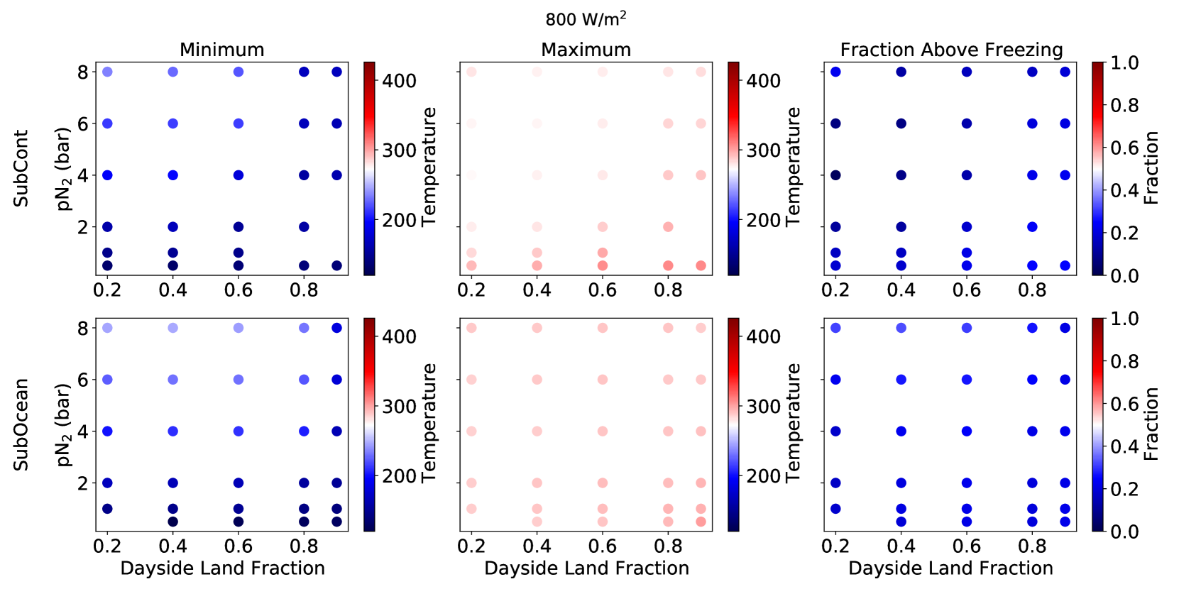
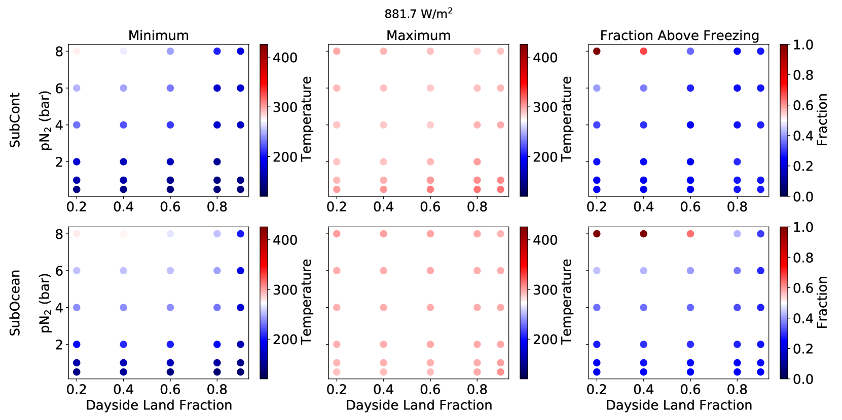
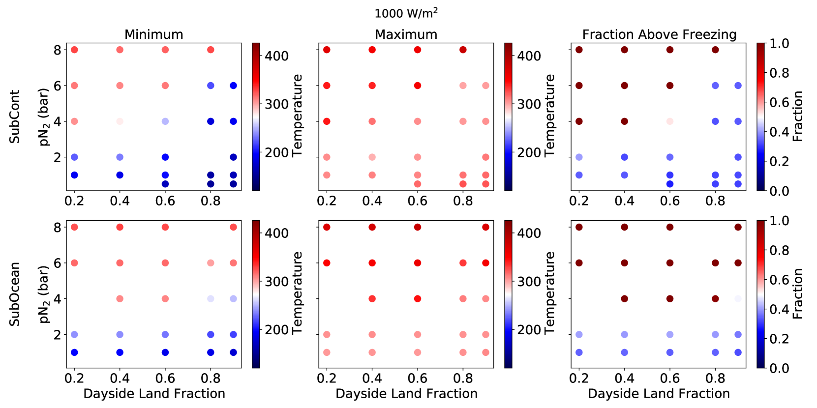
Figures 4, 5, 6, and 7 show the minimum and maximum surface temperature, and the fraction of the planet above the freezing point of water, for SubCont and SubOcean simulations with instellations of 800, 881.7, 900, and 1000 W/m², respectively. We use fraction above freezing rather than sea ice cover for consistency between planets with different landmaps; since SubOcean planets have nightside land, they cannot have nightside sea ice even when their nightsides are below freezing.

Figure 4: Left to right: minimum and maximum surface temperature and fraction above freezing for SubCont (top row) and SubOcean (bottom row) simulations with an incident flux of 700 W/m². The low-pN₂ models have the largest surface temperature ranges. Several high-pN₂ models of both landmap classes have maximum surface temperatures below freezing, meaning that they are in a snowball state.

Figure 5: Left to right: minimum and maximum surface temperature and fraction above freezing for SubCont (top row) and SubOcean (bottom row) simulations with an incident flux of 800 W/m². The low-pN₂ models again have the largest temperature ranges. In particular, SubCont models have both lower minimum and higher maximum surface temperatures at low pN₂ due to the reduced heat transport of the thinner atmospheres. This effect is less pronounced on SubOcean models due to the presence of dayside ocean.

Figure 6: Left to right: minimum and maximum surface temperature and fraction above freezing for SubCont (top row) and SubOcean (bottom row) simulations with an incident flux of 881.7 W/m². Only the highest-pN₂, lowest-land-fraction models are in the temperate nightside regime. These have minimum surface temperatures above freezing and substantially reduced day-night temperature contrasts.

Figure 7: Left to right: minimum and maximum surface temperature and fraction above freezing for SubCont (top row) and SubOcean (bottom row) simulations with an incident flux of 1000 W/m². The high-pN₂ models are in the temperate nightside regime, with the entire planet above freezing. The threshold for the transition to this regime is at higher pN₂ for high-land-fraction SubCont models because their atmospheres are drier.

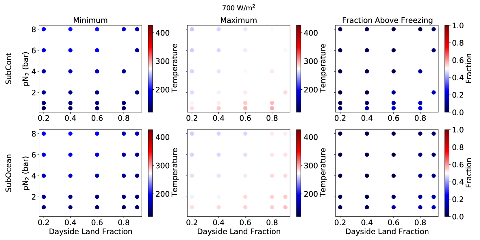
At 700 W/m², simulations are either snowballs (maximum surface temperature below freezing) or eyeballs (frozen nightside with a region above freezing on the dayside). High-pN₂ and low-land-fraction planets are in a snowball state, since these conditions allow more heat redistribution to the nightside. Low-pN₂ and high-land-fraction planets of both landmap types are in an eyeball state, with colder nightsides, warmer daysides, and a deglaciated substellar region. This trend suggests that the outer edge of the habitable zone is at lower instellations for high-land-fraction planets with thin atmospheres than for aquaplanets or those with high pN₂, since reduced heat transport in the former case keeps the substellar region habitable.

All 800 W/m² simulations are in the eyeball regime. These planets are relatively cold and dry. Their deglaciated substellar regions vary in size. As in previous studies, some simulations have dayside ice-free ocean, but high-land-fraction SubCont models do not. As with the 700 W/m² simulations, maximum surface temperature decreases as pN₂ increases, such that the substellar region is barely above freezing for low-land-fraction, high-pN₂ planets due to the increased nightward heat transport of their thicker atmospheres.

Most of the 881.7 W/m² simulations are eyeball climates, with the exception of some with low land fraction and high pN₂, which are in the transition or temperate nightside regime. The nightsides are cold at low pN₂ and high land fraction, especially for SubCont simulations, due to their drier atmospheres.

At 1000 W/m², many more simulations are in the temperate nightside or transition regime,. As before, high pN₂ and low dayside land fraction contribute to nightward heat transport. The dependence of the threshold pN₂ on land cover is highlighted for these hotter climates. SubOcean simulations transition to the temperate nightside regime more easily than SubCont simulations because of the difference in land position between these landmap classes. However, at this high instellation, all simulations with a pN₂ of 8 bars are in the temperate nightside regime regardless of land fraction.

4 Transition Validation

The eyeball and snowball regimes have been studied extensively (e.g., Pierrehumbert 2011; Checlair et al. 2017, 2019; Komacek & Abbot 2019; Yang et al. 2019; Sergeev et al. 2022; Turbet et al. 2022). The transition and temperate nightside regimes have been seen in other work (Paradise et al., 2022; Haqq-Misra et al., 2022), but have not been studied in as much detail. This section uses tests of atmospheric drag, water vapour, radiation balance, and cycling between climate states to isolate mechanisms involved in the transition.

4.1 Drag

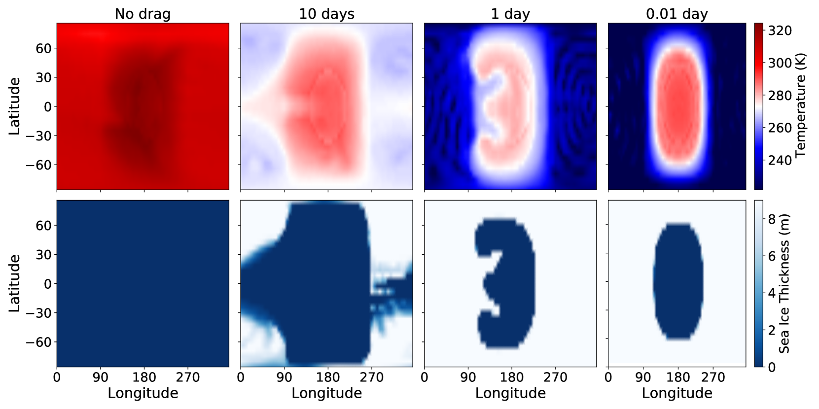
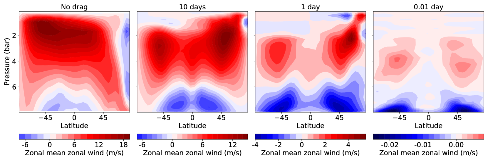
We identify advection as a driver of the climate transition by imposing an artificial drag to inhibit circulation. This term, which is not included in the default configuration, causes the horizontal winds to decay with a specified timescale $\tau_{drag}$ at all vertical levels. Our control simulation is a SubCont planet with with 20% dayside land cover, 8 bars of N₂, and an instellation of 881.7 W/m², run at a resolution of T21. Without artificial drag, this planet is in the temperate nightside climate regime. We run three new versions of this simulation with different values of $\tau_{drag}$ and find that the zonal mean zonal wind speeds decrease with decreasing values of $\tau_{drag}$ (Figure 9). These test cases result in a transition climate at a $\tau_{drag}$ of 10 days and eyeball climates with $\tau_{drag}$ of 1 and 0.01 days, with a much larger day-night temperature contrast in the latter case (Figure 8). This result points to horizontal advection from the dayside to the nightside as a driver of the high-pN₂ climate transition.

Figure 8: Surface temperature and sea ice thickness for simulations with varying drag timescales (column titles), for a SubCont planet with 20% dayside land, 8 bars of N₂, and an instellation of 881.7 W/m². As the drag timescale decreases, heat transport to the nightside is inhibited and the planet remains in an eyeball state, which suggests that advection plays an important role in the climate transition.

Figure 9: Zonal mean zonal wind for a SubCont planet with 20% dayside land, 8 bars of N₂, and an instellation of 881.7 W/m². Wind speeds are greatly reduced when a drag is applied (column titles), leading to decreased advection of heat to the nightside.

4.2 Water Vapour

To investigate the role of water vapour in heat transport, we run a simulation with surface evaporation turned off, such that there is water in the ocean, but it does not enter the atmosphere. We use the drag-free temperate nightside SubCont planet from Section 4.1. Figure 10 compares surface temperature maps for the wet and dry atmosphere simulations. The dry version remains in the eyeball state, with a completely frozen nightside and a partially deglaciated dayside, including some ice-free ocean.

Figure 10: Surface temperature comparison between default and dry-atmosphere runs of a SubCont model with a pN₂ of 8 bars, instellation of 881.7 W/m², and 20% dayside land cover. The default version is in the temperate nightside regime, whereas the dry version is in the eyeball regime with very cold nightside temperatures.

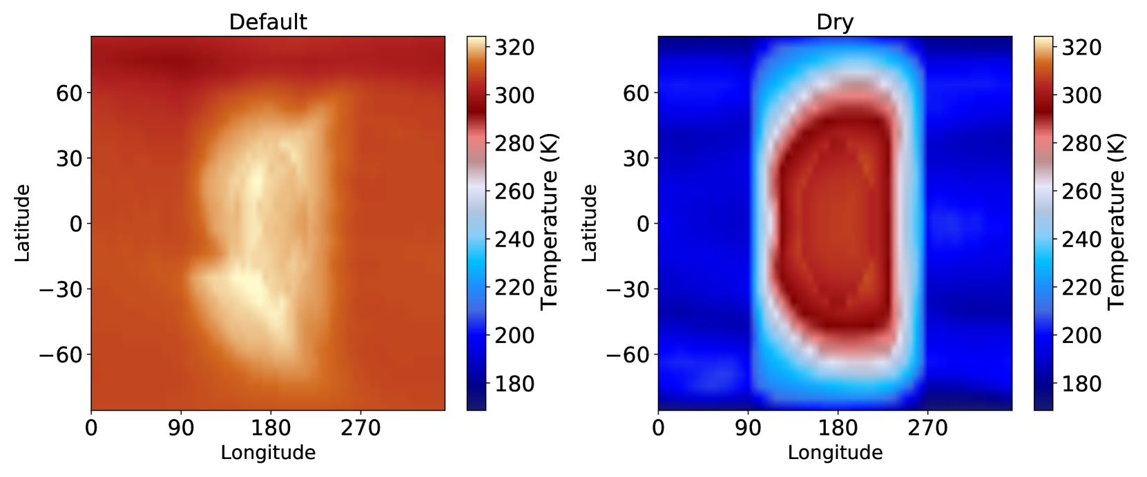
Water vapour plays a role in heat transport through evaporation from the dayside, advection to the nightside, and precipitation. It also contributes to the radiation balance by absorbing incident stellar radiation and outgoing longwave radiation emitted by the surface. These tests show that both advection and water vapour are required for the climate transition to the temperate nightside regime.

4.3 Radiation Balance

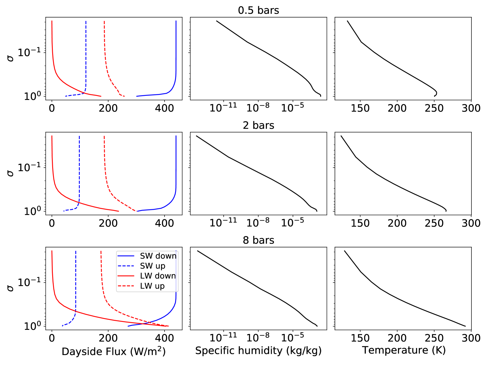
We compare the shortwave and longwave fluxes at each vertical level to understand where in the atmosphere the energy is being absorbed (Figure 11). Shortwave here corresponds to incident energy from the star, and longwave to energy emitted by the planet or its atmosphere. More shortwave energy is absorbed higher in the atmosphere as the pN₂ increases. The atmosphere is also more opaque to longwave radiation at high pN₂. This stronger greenhouse effect results in a warmer surface.

4.4 Stratospheric Humidity

Hot planets with significant water vapour in their atmospheres are at risk of entering an uninhabitable moist greenhouse state, in which water vapour enters the stratosphere and can then be lost to space. Kasting et al. (1993) define a moist greenhouse limit as stratospheric humidity exceeding $3\times 10^{-3}$ kg/kg, although this threshold can vary (Wordsworth & Pierrehumbert, 2014). Our simulations do not have a stratosphere, so we instead look at the maximum value of specific humidity in the highest layer of the atmosphere. This value is on the order of $10^{-6}$ kg/kg for our wettest climates, and is several orders of magnitude lower in the majority of our simulations, so we conclude that these climates are not in a moist greenhouse state.

4.5 Climate Cycling

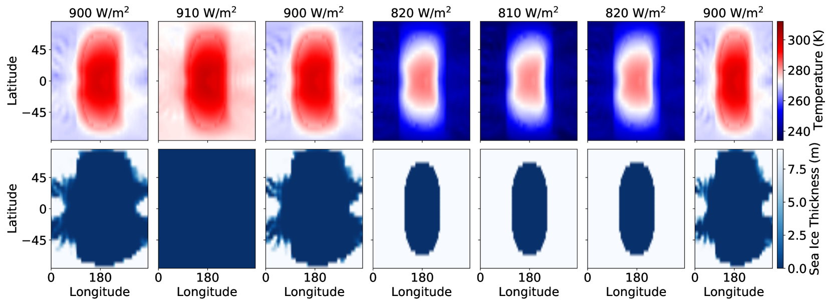
To investigate whether there are multiple stable climate states for a given configuration, we gradually perturb the instellation or pCO₂ of a simulation. We run these simulations at a resolution of T21 to allow them to reach an equilibrium state after each perturbations over several thousand years of total simulation time. We use a SubCont planet with 60% dayside land cover, a pN₂ of 6 bars, and an instellation of 900 W/m². This simulation is initially in the transition regime. A similar planet with either a lower land fraction, a higher pN₂, or a higher instellation would be in the temperate nightside regime, while one with a higher land fraction or a lower pN₂ or instellation would be in the eyeball regime.

Figure 11: Dayside average fluxes, specific humidity, and temperature profiles (columns) for simulations with varying pN₂ (rows). The high-pN₂ planet is hotter and wetter. It also absorbs and releases energy higher in its atmosphere. Note that the y-axis is in $\sigma$ coordinates, where $\sigma=P/P_{0}$ for pressure level $P$ and surface pressure $P_{0}$, rather than total pressure.

To test this planet’s climate sensitivity and stability, we run an initial simulation with the above parameters for 400 years, which is longer than the typical time required to reach energy balance equilibrium, in order to obtain an initial stable climate state in the transition regime. We then increase the pCO₂ by 200 $\mu$bar or the instellation by 10 W/m² and run the simulation for another 400 years, which results in a different stable climate state. We continue to increase the pCO₂ in steps of 200 $\mu$bar or the instellation in steps of 10 W/m², running for 400 years at each step, until the planet reaches the temperate nightside regime, with no sea ice. We then decrease the pCO₂ or instellation in the same manner until the ocean is completely ice-covered. We then reverse the sign of the perturbation again to return the climate to the temperate nightside state.

Figure 12 shows the sea ice fraction, average surface temperature, and atmosphere water vapour content for the pCO₂ perturbation cycle described above. The ice cover is most sensitive to pCO₂ around the nightside ice transition. We do not observe a hysteresis: for each pCO₂, the climate reaches the same final state from both directions. However, we note that there is more climate variability in the transition regime, when the nightside is partially deglaciated. This may be due to the way ExoPlaSim handles sea ice: each grid cell must be either fully ice-covered or fully ice-free (Checlair et al., 2017). Fluctuations in ice cover are therefore expected as ocean cells near the freezing point alternate between ice-covered and ice-free between timesteps.

Figure 12: Left to right: pCO₂, sea ice fraction, globally averaged surface temperature, and globally averaged water vapour as a function of time for a SubCont planet with an instellation of 900 W/m² and 60% dayside land cover. The simulation is initialized with 1000 $\mu$bar of CO₂ and run for 400 years, at which point its nightside is partly ice-covered. We increment the pCO₂ in steps of 200 $\mu$bar per 400 simulation years. Line colours represent the pCO₂. There is no strong dependence of the climate state on initial conditions, but there is significantly more climate variability in the partially deglaciated states.

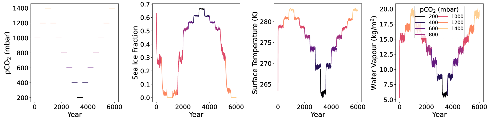
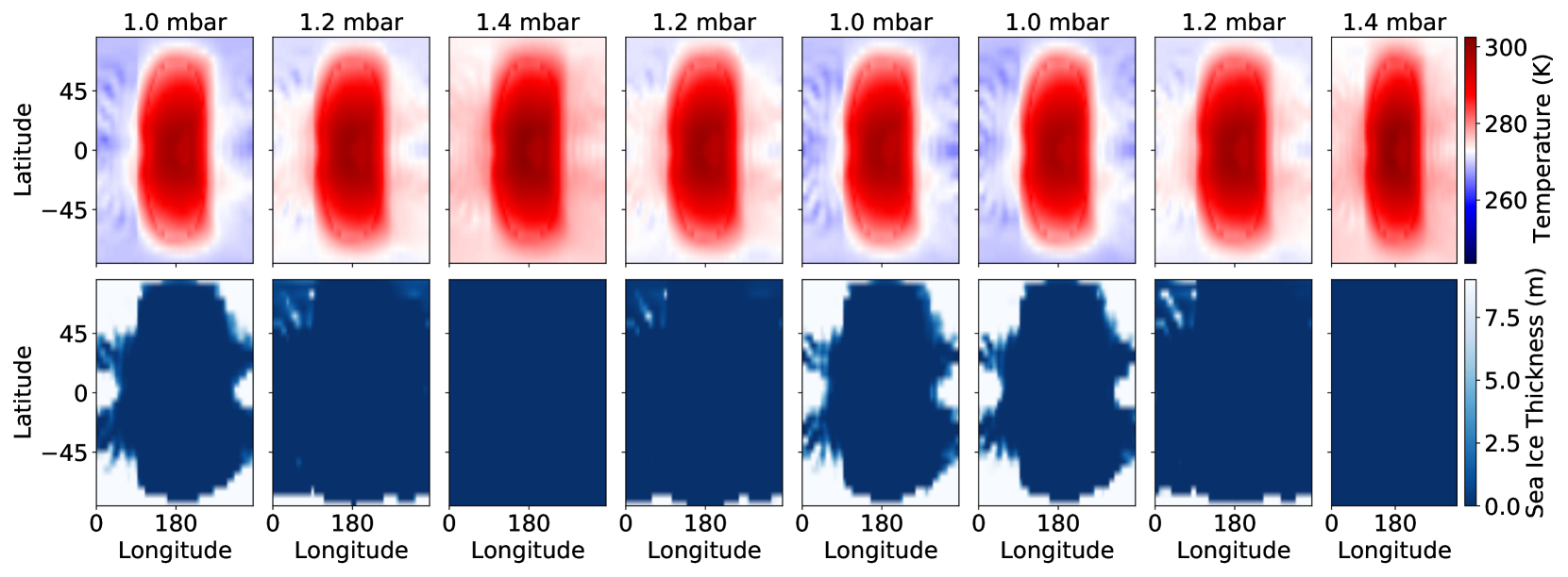
Figure 13 shows maps of equilibrium surface temperature and sea ice fraction for each cycle between the transition and temperate nightside regimes in Figure 12. We obtain one climate state per pCO₂ regardless of the direction of the perturbation.

Figure 13: Surface temperature (top row) and sea ice thickness (bottom row) for selected simulations from Figure 12. Column titles are the pCO₂. Each is shown at the end of the 400^th simulated year, right before the pCO₂ is perturbed again. Panels are in chronological order from left to right, with some simulations omitted. At a given pCO₂, the climate always reaches a nearly identical equilibrium state, regardless of whether the preceding state was warmer or colder.

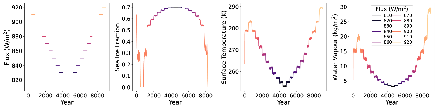
Figures 14 and 15 show the climate trends and maps for the instellation perturbation experiment. Again, the climate cycles smoothly between states, with more instability in partially deglaciated states. The climate is most sensitive to changes in instellation around the transition regime: there is a difference of only 20 W/m² between temperate nightside and eyeball states, whereas going from the transition regime to a fully ice-covered ocean requires further decreasing the instellation by 80 W/m².

Figure 14: Left to right: incident flux, sea ice fraction, globally averaged surface temperature, and globally averaged water vapour as a function of time for a SubCont planet with 60% dayside land cover, a constant pCO₂ of 1000 $\mu$bar and varying instellation in steps of $\pm 10$ W/m² every 400 simulation years. Line colours represent the incident flux. Again, there is no strong dependence of the climate state on initial conditions, but there is significantly more climate variability in the partially deglaciated states.

Figure 15: Surface temperature (top row) and sea ice thickness (bottom row) for selected simulations from Figure 14. Column titles are the instellation. Each is shown at the end of the 400^th simulated year, right before the instellation is perturbed again. Panels are in chronological order from left to right, with some simulations omitted. At a given instellation, the climate always reaches a nearly identical equilibrium state, regardless of whether the preceding state was warmer or colder.

Although these climate cycles are meant as a test of the robustness and stability of the climate states in these simulations, we note that a planet’s instellation, surface pressure, greenhouse gas abundance, and water availability are all subject to changes over the course of its evolution. These experiments strengthen the conclusions of Checlair et al. (2017, 2019), who found that synchronously rotating planets cycle smoothly between snowball and eyeball states, without a snowball bifurcation. They found that the ice albedo feedback is weaker on synchronous rotators than on Earth because the permanent nightside does not receive any direct incident stellar radiation, so the albedo of nightside snow and ice is irrelevant. We further note that the albedo of snow and ice is much lower in the infrared, where M-dwarfs emit more of their energy, so the feedback is further weakened compared to planets with a Sun-like stellar spectrum.

5 Impacts on Observations

At the time of writing, no atmospheres have yet been detected on M-Earths. Current and next-generation instruments will attempt to make such a detection over the coming years. In this section, we discuss how the large variety of climates presented in this paper would appear in transit and eclipse observations.

5.1 Transmission Spectroscopy

JWST will search for M-Earth atmospheres using transmission spectroscopy. These measurements are challenging because the signal from the planet’s atmosphere is small compared to stellar noise and other uncertainty sources. As seen in Figure 6 of Macdonald et al. (2024a), the high-pN₂, temperate nightside planets have the largest water vapour spectral features in synthetic transmission spectra, while low-pN₂, high-land-fraction planets have much smaller transit signals.

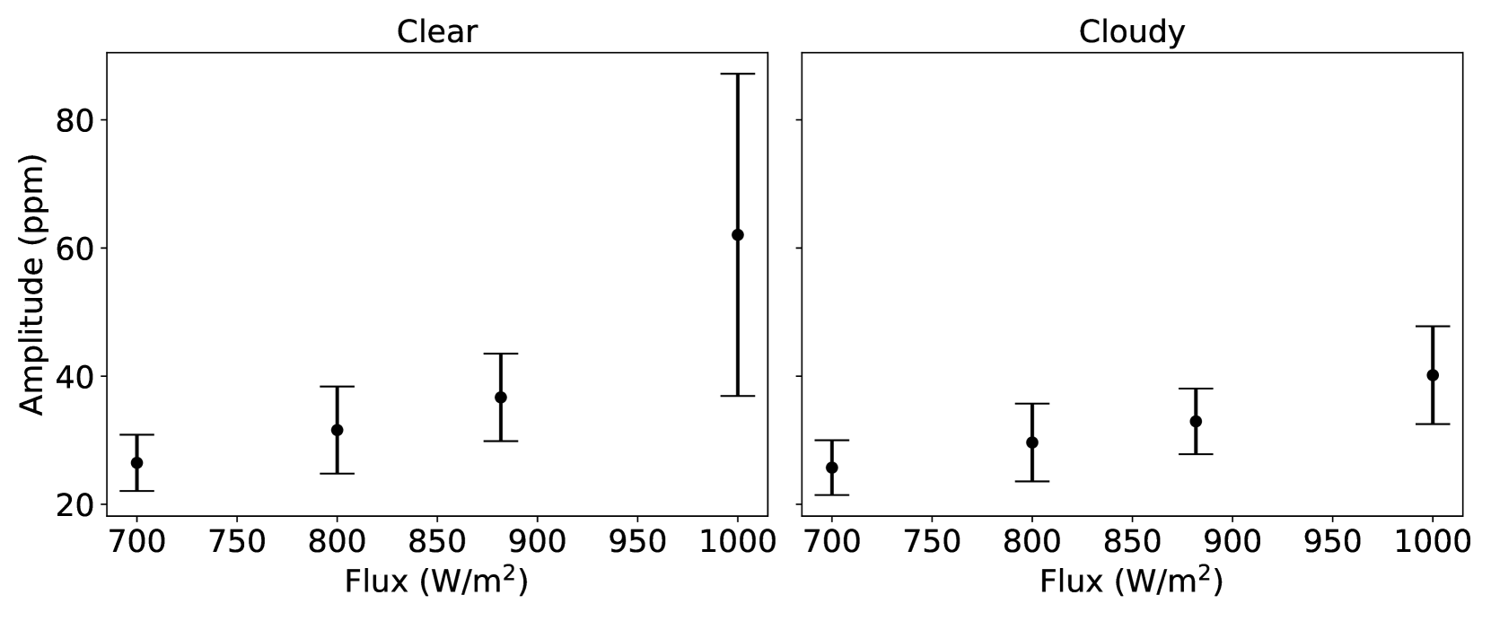
This trend is even more apparent with the range of incident fluxes in the present study’s simulations. Figure 16 shows the average water vapour amplitude as a function of incident flux for clear and cloudy conditions. As in Macdonald et al. (2024a), synthetic spectra are produced with petitRADTRANS (Mollière et al., 2019), with water vapour as the only absorber, and the amplitude is defined as the maximum differential transit depth of the $\sim$6 $\mu$m H₂O spectral feature. We find that a higher flux corresponds to both larger amplitudes and a larger spread, but that this spread is greatly reduced when clouds are included because they truncate the spectra higher up.

Figure 16: Water vapour transit amplitude in clear sky (left) and cloudy (right) synthetic spectra. Points are the average amplitude for all of the simulations of the corresponding flux, and error bars represent the standard deviation. Higher-instellation planets span a larger range of amplitudes, and are more affected by clouds, because these climates are warmer and wetter and have cloudier terminators.

5.2 Phase Curves

It is also relevant to consider whether M-Earth climate regimes could be identified using thermal phase curves. These observations measure the planet’s flux over a full orbital period, and therefore can provide temperature information. The phase curve amplitude is related to the day-night temperature contrast, which depends on the planet’s climate regime.

Previous studies have used simple models of synthetic M-Earth phase curves for different climate states. Yang et al. (2013) found differences in phase curve amplitude and shape for slow rotators with different atmospheres and fluxes. They found that clouds cause large differences in hotspot offset for high-instellation cases. Haqq-Misra et al. (2018) found that phase curves could be used to differentiate between rotation-related climate regimes, with rapid rotators exhibiting smaller phase curve amplitudes and shifted hotspots. Komacek & Abbot (2019) compared theoretical bolometric phase curves calculated from the upwelling top-of-atmosphere longwave flux for M-Earths with a range of star temperatures and incident fluxes. They also found that high-instellation, rapidly rotating planets have much flatter phase curves and larger hotspot shifts than slower rotators with lower incident flux.

We generate simplified synthetic phase curves for the simulations in this paper, assuming no orbital inclination. The thermal emission at a given orbital phase, $\phi$, is the integrated top-of-atmosphere (TOA) outgoing longwave radiation (OLR) in the direction of the observer. The TOA OLR of each grid cell in the direction of the observer, $f(\theta_{i},\lambda_{j})$ is the OLR multiplied by the cosine of the angle $\alpha_{ij}$ from the cell to the centre of the visible hemisphere, which is centred at longitude $\lambda=\phi$ and latitude $\theta=0$:

$$f(\theta_{i},\lambda_{i},\phi)=OLR_{ij}\cos{\alpha(\theta_{i},\lambda_{j},\phi)}$$ (1)

where

$$\sin^{2}\alpha(\theta_{i},\lambda_{j},\phi)=\cos^{2}\theta\sin^{2}{(\lambda-\phi)}+\sin^{2}{\theta}.$$ (2)

The flux, $F(\phi)$, is then the weighted average of $f$ over the surface area of the visible hemisphere:

$$F(\phi)=\frac{\sum_{i,j}{f(\theta_{i},\lambda_{j}},\phi)dA_{ij}}{\sum_{i,j}\cos\alpha_{ij}dA_{ij}}$$ (3)

where $dA_{i,j}$ is the element of surface area for grid cell $(i,j)$.

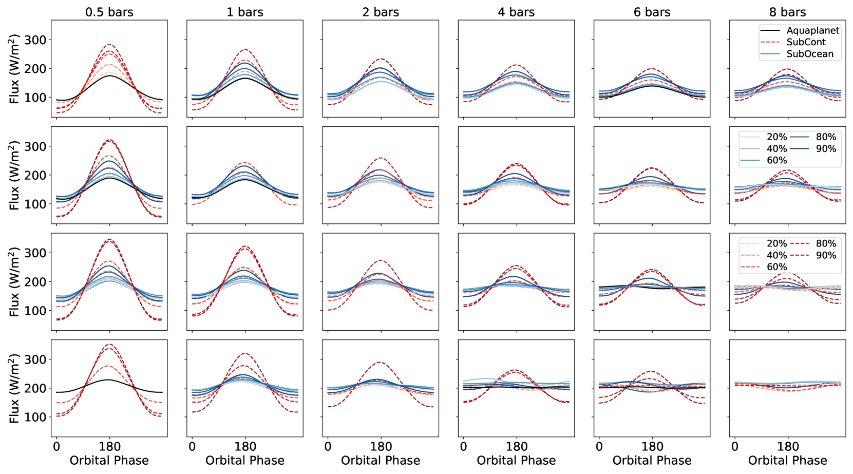
Figure 17 shows synthetic thermal phase curves for our set of simulations. Amplitudes are largest for planets with low pN₂ in the eyeball regime. Low-instellation, high-pN₂ snowballs have low overall fluxes and small amplitudes, as their dayside and nightside temperatures are cold. Temperate nightside planets exhibit much smaller amplitudes and larger hotspot offsets, similar to the rapid rotators of Haqq-Misra et al. (2018) and high-instellation planets of Komacek & Abbot (2019). However, rotation rate and instellation can be inferred from semi-major axis and stellar temperature for synchronous rotators, whereas pN₂ and land cover are unconstrained. Phase curve amplitude and shape may therefore provide more information about the latter two parameters.

Figure 17: Theoretical phase curves for planets with varying pN₂ and land cover. Top to bottom: instellations of 700, 800, 881.7, and 1000 W/m². Legend percentages indicate dayside land fraction. Secondary eclipse (dayside emission) is at an orbital phase of $\phi=180^{\circ}$. Planets with higher pN₂ have flatter phase curves, especially at 1000 W/m² where more of them are in the temperate nightside regime. However, the 700 W/m² high-pN₂ snowballs also have small amplitudes, so knowledge of instellation and overall planetary flux will be needed to distinguish between temperate nightside and snowball climates.

6 Discussion

We have shown using ExoPlaSim simulations that at sufficiently high instellation and pN₂, M-Earth climates transition from the eyeball regime with a frozen nightside to a “temperate nightside” climate regime in which the entire planet is above freezing, the day-night temperature differences are small, and the horizontal wind speeds are greatly reduced. We also find a “transition” climate regime between the eyeball and the temperate nightside, in which some nightside ice remains, particularly around the poles. The threshold pN₂ for a planet to transition at a given instellation is very sensitive to its land cover.

We have shown that this climate transition is driven by increased advection of heat to the nightside and heat transport by water vapour. We have found that the temperate nightside regime is stable, and shown that a planet can cycle back and forth between the eyeball and temperate nightside regimes in response to perturbations in instellation or pCO₂. We did not observe a snowball bifurcation, meaning that there is only one stable equilibrium climate state for a given combination of land cover, pN₂, pCO₂, and instellation; the planet will reach this equilibrium state from warmer or colder initial conditions. This result is relevant because a planet’s pN₂, pCO₂, and instellation can vary over time. Earth has some nitrogen stored in its mantle, and the pN₂ of its atmosphere is thought to have varied over geological timescales (Goldblatt et al., 2009). A planet may therefore be susceptible to transitions between climate regimes over geological timescales.

However, the equilibrium state for a given configuration is very sensitive to water availability and thus land cover. Because this climate transition relies on the presence of water vapour in the atmosphere, we would not expect it to occur in the same way on planets with low water inventories. These are more likely to remain in eyeball states.

We have also shown that cold climates are more likely to be in the snowball state at low land fraction or high pN₂ due to the increased advection of heat to the nightside by more massive atmospheres. This means that the outer edge of the habitable zone could be at higher instellation for thinner atmospheres, and is sensitive to dayside land fraction.

Paradise et al. (2021) used a Sun-like spectrum to model Earth-like and synchronously rotating planets with varying instellation and pN₂ with PlaSim. They found that the transition between an ice-free and ice-covered dayside for synchronous rotators, or between an ice-free and ice-covered entire planet for Earth-like rotators, spans a smaller instellation range at high pN₂. They attribute this effect to the decreasing surface temperature gradients with increasing pN₂. Similarly, we find that high-pN₂ planets go from snowballs at 700 W/m² to temperate nightsides at 1000 W/m², whereas lower-pN₂ planets are eyeballs through this entire instellation range.

Keles et al. (2018); Komacek & Abbot (2019); Paradise et al. (2021) found that for planets with Sun-like host stars, competition between Rayleigh scattering and pressure broadening causes a nonlinear temperature response to increasing pN₂, with the warming effect of pressure broadening dominating at low surface pressures and the cooling effect of Rayleigh scattering dominating at higher surface pressures. Keles et al. (2018) further showed that above 4 bars, when Rayleigh scattering is neglected, increasing pN₂ also has a net warming effect of increasing magnitude. Paradise et al. (2021) showed that when Rayleigh scattering is turned off, surface temperature increases monotonically with pN₂. Rayleigh scattering is much less important for the late M-dwarf host star used in our simulations, so the monotonic temperature increase we observe with increasing pN₂ is consistent with their results.

Our model atmospheres are composed of N₂ with trace CO₂ and H₂O. We have not included other trace gases or attempted to model atmospheric chemistry or aerosols. Keles et al. (2018) found, using a 1D climate model coupled to a chemistry model, that changes in pN₂ affect the vertical profiles and can enhance spectral features of trace gases in an Earth-like atmosphere with a Sun-like stellar spectrum. However, some of these spectral features are then obscured by the strong effects of pressure broadening on CO₂ and H₂O bands. A consistent chemistry model would be needed to understand these effects in M-Earth spectra. The results are also likely to be sensitive to the cloud parameterizations in both the GCM and the radiative transfer model.

Observations may eventually be able to differentiate between some of the more extreme climate states discussed in this paper. Temperate nightside climates exhibit small phase curve amplitudes and prominent transit water vapour features, attributed to their minimal temperature gradients and high water vapour content. In contrast, thin atmospheres and dry surfaces are associated with much larger phase curve amplitudes and significantly smaller water vapour transit signals. Our high-instellation simulations demonstrate the greatest variability in transit amplitude, a variability that is greatly reduced when clouds are included in the radiative transfer calculation.

The model planet used in this paper is small, to optimize its atmosphere for transmission spectroscopy. Phase curves would be easier to observe on a larger planet. Larger day-night temperature contrasts would also be expected in that case.

A mission sensitive to longer wavelengths, such as MIRECLE (Mandell et al., 2022), would be able to detect and characterize M-Earth atmospheres using planetary infrared excess (Stevenson & Space Telescopes Advanced Research Group on the Atmospheres of Transiting Exoplanets, 2020). In this method, the planet and star are observed simultaneously at a wide range of infrared wavelengths, and both their fluxes are fitted to the resulting spectrum. The planet’s signal can then be isolated. The planet’s signal is stronger in the thermal infrared because it is cooler and therefore peaks at longer wavelengths than the star.

Data Availability

The simulations in this study and files needed to reproduce them are available in Borealis repositories (Macdonald et al., 2024b, c).

References

- Benneke & Seager (2012) Benneke, B., & Seager, S. 2012, ApJ, 753, 100, doi: 10.1088/0004-637X/753/2/100
- Checlair et al. (2017) Checlair, J., Menou, K., & Abbot, D. S. 2017, The Astrophysical Journal, 845, 132, doi: 10.3847/1538-4357/aa80e1
- Checlair et al. (2019) Checlair, J. H., Olson, S. L., Jansen, M. F., & Abbot, D. S. 2019, ApJ, 884, L46, doi: 10.3847/2041-8213/ab487d
- Chemke et al. (2016) Chemke, R., Kaspi, Y., & Halevy, I. 2016, Geophysical Research Letters, 43, 11,414, doi: https://doi.org/10.1002/2016GL071279
- Goldblatt et al. (2009) Goldblatt, C., Claire, M. W., Lenton, T. M., et al. 2009, Nature Geoscience, 2, 891, doi: 10.1038/ngeo692
- Hammond & Lewis (2021) Hammond, M., & Lewis, N. T. 2021, Proceedings of the National Academy of Science, 118, 2022705118, doi: 10.1073/pnas.2022705118
- Haqq-Misra et al. (2022) Haqq-Misra, J., Wolf, E. T., Fauchez, T. J., Shields, A. L., & Kopparapu, R. K. 2022, \psj, 3, 260, doi: 10.3847/PSJ/ac9479
- Haqq-Misra et al. (2018) Haqq-Misra, J., Wolf, E. T., Joshi, M., Zhang, X., & Kopparapu, R. K. 2018, ApJ, 852, 67, doi: 10.3847/1538-4357/aa9f1f
- Kaspi & Showman (2015) Kaspi, Y., & Showman, A. P. 2015, ApJ, 804, 60, doi: 10.1088/0004-637X/804/1/60
- Kasting et al. (1993) Kasting, J. F., Whitmire, D. P., & Reynolds, R. T. 1993, Icarus, 101, 108, doi: 10.1006/icar.1993.1010
- Keles et al. (2018) Keles, E., Grenfell, J. L., Godolt, M., Stracke, B., & Rauer, H. 2018, Astrobiology, 18, 116, doi: 10.1089/ast.2016.1632
- Komacek & Abbot (2019) Komacek, T. D., & Abbot, D. S. 2019, ApJ, 871, 245, doi: 10.3847/1538-4357/aafb33
- Kopparapu et al. (2014) Kopparapu, R. K., Ramirez, R. M., SchottelKotte, J., et al. 2014, ApJ, 787, L29, doi: 10.1088/2041-8205/787/2/L29
- Macdonald et al. (2024a) Macdonald, E., Menou, K., Lee, C., & Paradise, A. 2024a, MNRAS, 529, 550, doi: 10.1093/mnras/stae554
- Macdonald et al. (2024b) —. 2024b, ExoPlaSim models for “Water Vapour Transit Ambiguities for Habitable M-Earths”, V1, V1, Borealis, doi: 10.5683/SP3/MQVUFQ
- Macdonald et al. (2024c) —. 2024c, ExoPlaSim models for “Climate Transition to Temperate Nightside at High Atmosphere Mass”, V1, Borealis, doi: 10.5683/SP3/EYDDSL
- Macdonald et al. (2022) Macdonald, E., Paradise, A., Menou, K., & Lee, C. 2022, MNRAS, 513, 2761, doi: 10.1093/mnras/stac1040
- Mandell et al. (2022) Mandell, A. M., Lustig-Yaeger, J., Stevenson, K. B., & Staguhn, J. 2022, AJ, 164, 176, doi: 10.3847/1538-3881/ac83a5
- Mollière et al. (2019) Mollière, P., Wardenier, J. P., van Boekel, R., et al. 2019, A&A, 627, A67, doi: 10.1051/0004-6361/201935470
- Paradise et al. (2021) Paradise, A., Fan, B. L., Menou, K., & Lee, C. 2021, Icarus, 358, 114301, doi: 10.1016/j.icarus.2020.114301
- Paradise et al. (2022) Paradise, A., Macdonald, E., Menou, K., Lee, C., & Fan, B. L. 2022, MNRAS, 511, 3272, doi: 10.1093/mnras/stac172
- Pierrehumbert (2011) Pierrehumbert, R. T. 2011, ApJ, 726, L8, doi: 10.1088/2041-8205/726/1/L8
- Ramirez (2020) Ramirez, R. M. 2020, Monthly Notices of the Royal Astronomical Society, 494, 259, doi: 10.1093/mnras/staa603
- Sergeev et al. (2022) Sergeev, D. E., Fauchez, T. J., Turbet, M., et al. 2022, Planetary Science Journal, 3, 212, doi: 10.3847/PSJ/ac6cf2
- Stevenson & Space Telescopes Advanced Research Group on the Atmospheres of Transiting Exoplanets (2020) Stevenson, K. B., & Space Telescopes Advanced Research Group on the Atmospheres of Transiting Exoplanets. 2020, ApJ, 898, L35, doi: 10.3847/2041-8213/aba68c
- Turbet et al. (2016) Turbet, M., Leconte, J., Selsis, F., et al. 2016, A&A, 596, A112, doi: 10.1051/0004-6361/201629577
- Turbet et al. (2022) Turbet, M., Fauchez, T. J., Sergeev, D. E., et al. 2022, Planetary Science Journal, 3, 211, doi: 10.3847/PSJ/ac6cf0
- Wordsworth (2016) Wordsworth, R. 2016, Earth and Planetary Science Letters, 447, 103, doi: https://doi.org/10.1016/j.epsl.2016.04.002
- Wordsworth & Pierrehumbert (2014) Wordsworth, R., & Pierrehumbert, R. 2014, ApJ, 785, L20, doi: 10.1088/2041-8205/785/2/L20
- Xiong et al. (2022) Xiong, J., Yang, J., & Liu, J. 2022, Geophys. Res. Lett., 49, e99599, doi: 10.1029/2022GL099599
- Yang et al. (2013) Yang, J., Cowan, N. B., & Abbot, D. S. 2013, ApJ, 771, L45, doi: 10.1088/2041-8205/771/2/L45
- Yang et al. (2019) Yang, J., Leconte, J., Wolf, E. T., et al. 2019, ApJ, 875, 46, doi: 10.3847/1538-4357/ab09f1
- Zhang & Yang (2020) Zhang, Y., & Yang, J. 2020, ApJ, 901, L36, doi: 10.3847/2041-8213/abb87f