Inversion diameter and treewidth

Abstract

In an oriented graph $\overrightarrow{G}$, the inversion of a subset $X$ of vertices is the operation that reverses the orientation of all arcs with both end-vertices in $X$. The inversion graph of a graph $G$, denoted by $\mathcal{I}(G)$, is the graph whose vertices are orientations of $G$ in which two orientations $\overrightarrow{G_{1}}$ and $\overrightarrow{G_{2}}$ are adjacent if and only if there is an inversion transforming $\overrightarrow{G_{1}}$ into $\overrightarrow{G_{2}}$. The inversion diameter of a graph $G$ is the diameter of its inversion graph $\mathcal{I}(G)$, denoted by $\operatorname{\mathrm{diam}}(\mathcal{I}(G))$. Havet, Hörsch, and Rambaud (2024) first proved that for $G$ of treewidth $k$, $\operatorname{\mathrm{diam}}(\mathcal{I}(G))\leq 2k$, and that there are graphs of treewidth $k$ with inversion diameter $k+2$. In this paper, we construct graphs of treewidth $k$ with inversion diameter $2k$, which implies that the previous upper bound $\operatorname{\mathrm{diam}}(\mathcal{I}(G))\leq 2k$ is tight. Moreover, for graphs with maximum degree $\Delta$, Havet, Hörsch, and Rambaud (2024) proved $\operatorname{\mathrm{diam}}(\mathcal{I}(G))\leq 2\Delta-1$ and conjectured that $\operatorname{\mathrm{diam}}(\mathcal{I}(G))\leq\Delta$. We prove the conjecture when $\Delta=3$ with the help of computer calculations.

Keywords: inversion diameter; orientation; treewidth.

1 Introduction

An orientation of an undirected graph is an assignment of a direction to each edge, turning the initial graph into a directed graph. Let $G$ be a simple graph and $\overrightarrow{G_{1}}$ an orientation of $G$. If $X$ is a vertex subset of $G$, the inversion of $X$ on $\overrightarrow{G_{1}}$ is the operation that reverses the direction of all arcs with both end-vertices in $X$, and results in a new orientation $\overrightarrow{G_{2}}$.

The concept of inversion was first introduced by Belkhechine et al. [4]. They studied the inversion number of a directed graph $D$, denoted by $\operatorname{\mathrm{inv}}(D)$, which is the minimum number of inversions that transform $D$ into an acyclic graph. They proved, for every fixed $k$, given a tournament $T$, determining whether $\operatorname{\mathrm{inv}}(T)\leq k$ is polynomial-time solvable. In contrast, Bang-Jensen et al. [3] proved that given any directed graph $D$, determining whether $\operatorname{\mathrm{inv}}(D)\leq 1$ is NP-complete.

The maximum inversion number across all oriented graphs of order $n$, denoted by $\operatorname{\mathrm{inv}}(n)$, has also been investigated. Aubian et al. [2] and Alon et al. [1] proved $n-2\sqrt{2\log n}\leq\operatorname{\mathrm{inv}}(n)\leq n-\lceil\log(n+1)\rceil$. Besides these results, various related questions have also been studied.

Let $G$ be a simple graph. An inversion is a transformation between different orientations of $G$. Instead of transforming an orientation into an acyclic orientation, it is also natural to consider the inversion between two orientations. The inversion graph of $G$ denoted by $\mathcal{I}(G)$, is the graph whose vertices are the orientations of $G$ in which two orientations $\overrightarrow{G_{1}}$ and $\overrightarrow{G_{2}}$ are adjacent if and only if there is an inversion $X$ transforming $\overrightarrow{G_{1}}$ into $\overrightarrow{G_{2}}$. The inversion diameter of $G$ is the diameter of $\mathcal{I}(G)$, denoted by $\operatorname{\mathrm{diam}}(\mathcal{I}(G))$. It represents the maximum number of inversions required to transform an orientation of $G$ into another.

Havet et al. [5] first introduced inversion diameter and studied its behaviour on various classes of graphs. Let $G$ be a graph and let $<$ be a total ordering on $V(G)$. For every pair $u,u^{\prime}$ of vertices in $G$, let $N_{<u^{\prime}}(u)=\{v\in N(u)\mid v<u^{\prime}\}$ and $N_{>u^{\prime}}(u)=\{v\in N(u)\mid v>u^{\prime}\}$. We simply write $N_{<}(u)$ for $N_{<u}(u)$ and $N_{>}(u)$ for $N_{>u}(u)$. The ordering $<$ is $t$-strong if for every $u\in V(G)$

• $|N_{<}(u)|+\log(|\{X\subseteq V(G)\mid\exists v\in N_{>}(u),X\subseteq N_{<u}(v)\}|)<t$, if $N_{>}(u)\neq\emptyset$, and

• $N_{<}(u)\leq t$ otherwise.

A graph is strongly $t$-degenerate if it admits a $t$-strong ordering of its vertices. Havet et al. [5] showed that

Theorem 1.1 (Havet et al. [5])

Let $G$ be a graph and let $t$ be a positive integer. If $G$ is strongly $t$-degenerate, then $\operatorname{\mathrm{diam}}(\mathcal{I}(G))\leq t$.

As corollaries of Theorem 1.1, they showed that various properties of a graph can be used to bound the diameter of its inversion graph.

Theorem 1.2 (Havet et al. [5])

1. For every graph $G$ with at least one edge and maximum degree $\Delta$, $\operatorname{\mathrm{diam}}(\mathcal{I}(G))\leq 2\Delta-1$.

2. $\operatorname{\mathrm{diam}}(\mathcal{I}(G))\leq 12$ for every planar graph $G$.

3. $\operatorname{\mathrm{diam}}(\mathcal{I}(G))\leq 2k$ for every graph $G$ of treewidth at most $k$.

Havet et al. [5] also proved that for fixed $k\geq 2$, given a graph $G$, determining whether $\operatorname{\mathrm{diam}}(\mathcal{I}(G))\leq k$ is NP-hard. For a graph $G$ with maximum degree $3$ (a sub-cubic graph), Havet et al. [5] showed a better bound $\operatorname{\mathrm{diam}}(\mathcal{I}(G))\leq 4$. Moreover, they proposed the following conjecture on graphs with maximum degree $\Delta$.

Conjecture 1.3 (Havet et al. [5])

For every graph $G$ with at least one edge and maximum degree $\Delta$, $\operatorname{\mathrm{diam}}(\mathcal{I}(G))\leq\Delta$.

The conjecture is true for $\Delta\leq 2$ [5]. In this paper, we prove the conjecture when $\Delta=3$. Computer assistance will be used in the proof of Theorem 1.4. A pure mathematical proof is still worth studying.

Theorem 1.4

If $G$ is a graph of maximum degree $3$, then $\operatorname{\mathrm{diam}}(\mathcal{I}(G))\leq 3$.

For graphs with treewidth at most $k$, Havet et al. [5] showed that there are graphs of treewidth at most $k$ with inversion diameter $k+2$. In this paper, we show that the upper bound $\operatorname{\mathrm{diam}}(\mathcal{I}(G))\leq 2k$ for graphs of treewidth at most $k$ is tight by proving Theorem 1.5. In doing so, we answer a question proposed by Havet et al. in [5].

Theorem 1.5

For every positive integer $k$, there are graphs of treewidth $k$ with inversion diameter $2k$.

This paper is organized as follows. In Section 2, we give basic definitions and notation. The proofs of Theorems 1.5 and 1.4 are given in Sections 3 and 4, respectively.

2 Preliminaries

Let $G=(V,E)$ be a graph. The distance between $u$ and $v$, denoted by $\operatorname{\mathrm{dist}}(u,v)$, is the number of edges in a shortest path joining $u$ and $v$. For any vertex $u\in V(G)$, let $N(u)=\{v\mid uv\in E(G)\}$ and denote by $d(u)=|N(u)|$ the degree of $u$. Let $\Delta(G)$ be the maximum degree of $G$. We call $G$ $k$-regular if $d(u)=k$ for every $u\in V(G)$. Let $G$ be a graph and $S$ a vertex subset of its vertices. Let $G[S]$ denote the subgraph of $G$ induced by $S$. For a graph $G$ and a vertex $v$, denote by $G-v$ the graph induced by $V(G)-\{v\}$. For a graph $G$ and an induced subgraph $H$, denote by $G-H$ the graph induced by $V(G)-V(H)$.

A labelling of $G$ is a mapping $\pi:E(G)\rightarrow\mathbb{F}_{2}$. A $t$-dim vector assignment of $G$ respecting the labelling $\pi$ is a mapping $f:V(G)\rightarrow\mathbb{F}_{2}^{t}$ such that $\pi(uv)=f(u)\cdot f(v)$ for every edge $uv\in E(G)$, where $f(u)\cdot f(v)$ is the scalar product of $f(u)$ and $f(v)$ over $\mathbb{F}_{2}^{t}$. Usually, we use the bold letter $\mathbf{u}$ to represent $f(u)$. We use $\mathbf{0}$ (resp. $\mathbf{1}$) to represent vectors in $\mathbb{F}_{2}^{t}$ whose coordinates are all $0$ (resp. $1$). We say a vector $\mathbf{u}\in\mathbb{F}_{2}^{t}$ is odd (resp. even), if $\mathbf{u\cdot 1}$ is one (resp. zero), i.e., $\mathbf{u}$ has an odd (resp. even) number of $1$s.

The inversion diameter has a close relation with vector assignment as given in the following proposition.

Proposition 2.1 ([5])

For every graph $G$ and every positive integer $t$, the following are equivalent.

1. $\operatorname{\mathrm{diam}}(\mathcal{I}(G))\leq t$.

2. For every labelling $\pi$, there exists a $t$-dim vector assignment of $G$ respecting the labelling $\pi$.

The treewidth of a graph $G$, denoted by $\operatorname{\mathrm{tw}}(G)$ can be defined in many ways. Here we give a definition of treewidth from the perspective of $k$-trees.

Definition 2.2

A graph $G$ is a $k$-tree if

1. it is a $k$-clique, or

2. there exists a vertex $v$ such that $N(v)$ is a $k$-clique, and $G-v$ is a k-tree.

We say a graph is a partial $k$-tree if it is a subgraph of a $k$-tree. It is known that a graph $G$ is a partial $k$-tree if and only if the treewidth of $G$ is at most $k$ [6, 7].

Let $\mathcal{L}(\mathbf{v}_{1},\ldots,\mathbf{v}_{k})$ denote the linear space spanned by $\mathbf{v}_{1},\ldots,\mathbf{v}_{k}$. For two vectors $\mathbf{v}$ and $\mathbf{u}$ in $\mathbb{F}_{2}^{t}$, we write $\mathbf{v\perp u}$ if $\mathbf{v\cdot u}=0$. For a vector $\mathbf{v}\in\mathbb{F}_{2}^{t}$ and a linear space $\mathbf{U}$ in $\mathbb{F}_{2}^{t}$, we write $\mathbf{v\perp U}$ if $\mathbf{v\perp u}$ for every $\mathbf{u\in U}$. The orthogonal complementary space of $\mathbf{U}$ is $\mathbf{U}^{\perp}=\{\mathbf{v}\mid\mathbf{v\perp U}\}$. For any positive integer $k$, we write $[k]=\{1,2,\ldots,k\}$.

Definition 2.3

We say the vectors $\mathbf{v}_{1},\ldots,\mathbf{v}_{k}$ are orthogonal if $\mathbf{v}_{i}\perp\mathbf{v}_{j}$ for all $i,j\in[k]$ with $i\neq j$. We say they are self-orthogonal if $\mathbf{v}_{i}\perp\mathbf{v}_{j}$ for all $i,j\in[k]$, that is, they are orthogonal and every vector is even.

Definition 2.4

A linear space $\mathbf{U}$ is self-orthogonal if $\mathbf{U\subseteq U^{\perp}}$.

Let $\mathbf{U}$ be a self-orthogonal linear space. Then $\mathbf{U}$ is orthogonal and every vector in $\mathbf{U}$ is even. It is easy to verify that $\mathbf{U}$ is self-orthogonal if and only if it has self-orthogonal base vectors.

For a linear space $\mathbf{U}$ and a vector $\mathbf{v}$, denote by $\mathbf{v+U}$ the set $\{\mathbf{v+u}\mid\mathbf{u\in U}\}$ and denote by $\mathcal{L}(\mathbf{U,v})$ the space spanned by $\mathbf{v}$ and a basis of $\mathbf{U}$, that is the summation space of $\mathbf{U}$ and $\mathcal{L}(\mathbf{v})$.

3 Proof of Theorem 1.5

For $k\geq 1$, we define a sequence of graphs $G_{i}^{(k)}$ respecting a fixed labelling $\pi_{i}^{(k)}$. First, let $G_{0}^{(k)}$ be a $k$-clique respecting an arbitrary labelling $\pi_{0}^{(k)}$. For convenience, we define $V(G^{(k)}_{-1})=\emptyset$. Then, we recursively construct $G_{i}^{(k)}$ as follows:

(i) for each $k$-clique with vertices $v_{1},\ldots,v_{k}$ in $G_{i-1}^{(k)}$ and each $\mathbf{x}={(x_{1},\ldots,x_{k})}^{T}\in\mathbb{F}_{2}^{k}$, we add a new vertex $u$ such that $uv_{j}\in E(G_{i}^{(k)})$ and $\pi_{i}^{(k)}(uv_{j})=x_{j}$, for all $1\leq j\leq k$;

(ii) $\pi^{(k)}_{i}|_{G^{(k)}_{i-1}}=\pi^{(k)}_{i-1}$.

Since $|\mathbb{F}_{2}^{k}|=2^{k}$, we add $2^{k}$ new vertices for each $k$-clique in $G_{i-1}^{(k)}$. Observe that every $p$-clique ($p<k$) in $G_{i}^{(k)}$ must be contained in a $k$-clique in $G_{i}^{(k)}$. By Definition 2.2, $G_{m}^{(k)}$ is a $k$-tree for every $m$, that is, of treewidth at most $k$. Since $\pi^{(k)}_{n}|_{G^{(k)}_{m}}=\pi^{(k)}_{m}$ when $n>m$, we may use $\pi^{(k)}$ to denote the labelling of $G^{(k)}_{m}$ for every $m$. For every vertex $v\in V(G^{(k)}_{m})$ with $m\geq 1$, there exists a unique $n$ such that $v\in V(G^{(k)}_{n})-V(G^{(k)}_{n-1})$. We say $n$ is the level of $v$, denoted by $l(v)=n$. For a vertex set $S\subseteq G^{(k)}_{m}$ with $m\geq 1$, the level of $S$ is defined to be the maximum level of a vertex in $S$ and it is denoted by $l(S)$, that is, $l(S)=\max_{v\in S}\{l(v)\}$. Clearly, if $v$ is a vertex in $G_{m}^{(k)}$, then $l(v)\leq m$. Similarly, if $C$ is a vertex set in $G_{m}^{(k)}$, then $l(C)\leq m$.

Note that if $H$ is a subgraph of $G$, then $\operatorname{\mathrm{diam}}(\mathcal{I}(H))\leq\operatorname{\mathrm{diam}}(\mathcal{I}(G))$. So ${(\operatorname{\mathrm{diam}}(\mathcal{I}(G_{m}^{(k)})))}_{m\geq 0}$ is an increasing sequence with upper bound $2k$ by Theorem 1.2.

Let $\lambda^{(k)}=\lim_{m\rightarrow+\infty}\operatorname{\mathrm{diam}}(\mathcal{I}(G_{m}^{(k)}))$. Then $\lambda^{(k)}\leq 2k$. We will show that $\lambda^{(k)}=2k$, that is, $G_{m}^{(k)}$ is of inversion diameter $2k$ when $m$ is sufficiently large.

Next we suppose that $\lambda^{(k)}\leq 2k-1$. Then for every $m$, $G_{m}^{(k)}$ has a $(2k-1)$-dim vector assignment respecting the labelling $\pi^{(k)}$ by Proposition 2.1. Thus for each $v\in V(G_{m}^{(k)})$, there is a vector $\mathbf{v}\in\mathbb{F}_{2}^{2k-1}$ corresponding to it. The following lemmas show the properties of the vectors assigned to $k$-cliques in $G^{(k)}_{m}$.

Lemma 3.1

If there is a $k$-clique of level $m$ with vertices $v_{1},\ldots,v_{k}$ in $G^{(k)}_{m+1}$, then $\mathbf{v}_{1},\ldots,\mathbf{v}_{k}$ are linearly independent.

Proof. Otherwise, without loss of generality, assume $\mathbf{v}_{1}=\sum_{i=2}^{k}c_{i}\mathbf{v}_{i}$ where $c_{i}\in\mathbb{F}_{2}$ for all $2\leq i\leq k$. By the construction, there exists a vertex $u\in V(G^{(k)}_{m+1})$ which is connected to $v_{2},\ldots,v_{k}$ with edges labelled by $1$, and to $v_{1}$ with an edge labelled by $\sum_{i=2}^{k}c_{i}+1$. Therefore,

$$\sum_{i=2}^{k}c_{i}+1 =\pi^{(k)}(uv_{1})=\mathbf{u}\cdot\mathbf{v}_{1}=\mathbf{u}\cdot\sum_{i=2}^{k}c_{i}\mathbf{v}_{i}=\sum_{i=2}^{k}c_{i}\mathbf{u}\cdot\mathbf{v}_{i}=\sum_{i=2}^{k}c_{i}\pi^{(k)}(uv_{i})=\sum_{i=2}^{k}c_{i},$$

a contradiction. $\square$

Lemma 3.2

If there is a $k$-clique in $G^{(k)}_{m+2}$ of level $m$ with vertices $v_{1},\ldots,v_{k}$, and $u$ is a vertex of level $m+1$ adjacent to all ${(v_{i})}_{1\leq i\leq k}$, then either $\mathbf{v}_{1},\ldots,\mathbf{v}_{k},\mathbf{u}$ are linearly independent, or $\mathbf{u}=\sum_{i=1}^{k}\mathbf{v}_{i}$.

Proof. Firstly, by Lemma 3.1, $\mathbf{v}_{1},\ldots,\mathbf{v}_{k}$ are linearly independent. Note that for every $1\leq j\leq k$, $v_{1},\ldots,v_{j-1},v_{j+1},\ldots,v_{k},u$ is also a $k$-clique of level $m+1$ in $G^{(k)}_{m+2}$. Then by Lemma 3.1, for every $1\leq j\leq k$, $\mathbf{v}_{1},\ldots,\mathbf{v}_{j-1},\mathbf{v}_{j+1},\ldots,\mathbf{v}_{k},\mathbf{u}$ are linearly independent. Assume $\mathbf{u}=\sum_{i=1}^{k}c_{i}\mathbf{v}_{i}$ where $c_{i}\in\mathbb{F}_{2}$ for all $1\leq i\leq k$. If $c_{j}=0$ for some $j$, then it contradicts that $\mathbf{v}_{1},\ldots,\mathbf{v}_{j-1},\mathbf{v}_{j+1},\ldots,\mathbf{v}_{k},\mathbf{u}$ are linearly independent. Therefore, $\mathbf{u}=\sum_{i=1}^{k}\mathbf{v}_{i}$. $\square$

Lemma 3.3

Let $v_{1},\ldots,v_{k}$ be vertices of a $k$-clique of level $m$ in $G^{(k)}_{m+2}$ and $\mathbf{A}={(\mathbf{v}_{1},\ldots,\mathbf{v}_{k})}^{T}$. Then for every $\mathbf{b}\in\mathbb{F}_{2}^{k}$, $\mathbf{Ax=b}$ has a solution $\mathbf{y}$ such that either $\mathbf{v}_{1},\ldots,\mathbf{v}_{k},\mathbf{y}$ are linearly independent, or $\mathbf{y}=\sum_{i=1}^{k}\mathbf{v}_{i}$.

Proof. Let $\mathbf{b}={(b_{1},\ldots,b_{k})}^{T}$. By construction, there exists a vertex $u\in V(G^{(k)}_{m+1})$ of level $m+1$ connecting ${(v_{i})}_{1\leq i\leq k}$ such that $\pi^{(k)}(uv_{i})=b_{i}$ for all $1\leq i\leq k$. Then we have $\mathbf{Au=b}$. By Lemma 3.2, either $\mathbf{v}_{1},\ldots,\mathbf{v}_{k},\mathbf{u}$ are linearly independent, or $\mathbf{u}=\sum_{i=1}^{k}\mathbf{v}_{i}$. $\square$

The above actually work for arbitrary $\lambda^{(k)}$, while the following lemmas need the assumption $\lambda^{(k)}\leq 2k-1$.

Lemma 3.4

Let $v_{1},\ldots,v_{k}$ be vertices of a $k$-clique of level $m$ in $G^{(k)}_{m+2}$ and $\mathbf{A}={(\mathbf{v}_{1},\ldots,\mathbf{v}_{k})}^{T}$. Then $\mathbf{Ax=0}$ has a solution $\mathbf{y}$ such that $\mathbf{v}_{1},\ldots,\mathbf{v}_{k},\mathbf{y}$ are linearly independent.

Proof. We prove it by contradiction. By Lemma 3.1, $\mathbf{v}_{1},\ldots,\mathbf{v}_{k}$ are linearly independent. Let $\mathbf{U}$ be the solution space of $\mathbf{Ax=0}$. Suppose $\mathbf{U}$ is a subspace of $\mathcal{L}(\mathbf{v}_{1},\ldots,\mathbf{v}_{k})$, otherwise we can pick $\mathbf{y}$ from $\mathbf{U}-\mathcal{L}(\mathbf{v}_{1},\ldots,\mathbf{v}_{k})$ and then $\mathbf{v}_{1},\ldots,\mathbf{v}_{k},\mathbf{y}$ are linearly independent. Since $\mathbf{A}$ is a $k\times(2k-1)$ matrix, $\dim(\mathbf{U})=(2k-1)-k=k-1$. By setting $\mathbf{b=0}$ in Lemma 3.3, we have $\sum_{i=1}^{k}\mathbf{v}_{i}\in\mathbf{U}$.

For each $j\in[k]$, the solution set of $\mathbf{Ax=A}\mathbf{{}v}_{j}$ is in $\mathbf{v}_{j}+\mathbf{U}\subseteq\mathcal{L}(\mathbf{v}_{1},\ldots,\mathbf{v}_{k})$. Then any solution of $\mathbf{Ax=A}\mathbf{v}_{j}$ cannot be independent from $\mathbf{v}_{1},\ldots,\mathbf{v}_{k}$. By Lemma 3.3, there is a solution $\mathbf{y}$ such that either $\mathbf{v}_{1},\ldots,\mathbf{v}_{k},\mathbf{y}$ are linearly independent, or $\mathbf{y}=\sum_{i=1}^{k}\mathbf{v}_{i}$. Since every solution is in $\mathbf{v}_{j}+\mathbf{U}\subseteq\mathcal{L}(\mathbf{v}_{1},\dots,\mathbf{v}_{k})$, the first outcome does not occur, and so $\sum_{i=1}^{k}\mathbf{v}_{i}\in\mathbf{v}_{j}+\mathbf{U}$. Therefore, $\mathbf{v}_{j}\in\mathbf{U}$ for every $1\leq j\leq k$, which contradicts that $\dim(\mathbf{U})=k-1$ because $\mathbf{v}_{1},\ldots,\mathbf{v}_{k}$ are linearly independent. $\square$

Definition 3.5

Let $C$ be a $p$-clique of $G^{(k)}_{m}$ for some $m$. $C$ is called a bad clique if $\dim(\textbf{V}_{C}\cap\textbf{V}_{C}^{\perp})\geq p-1$, where $\textbf{V}_{C}=\mathcal{L}(\{\mathbf{v}\mid v\in C\})$ and $p\geq 1$.

Note that a single vertex is always a bad $1$-clique. If $\lambda^{(k)}\leq 2k-1$, “large” bad cliques will finally cause contradictions. The following lemma is the main part of our proof which states that we can find a “large” bad clique when $m$ is sufficiently large.

Lemma 3.6

If there exists a bad $p$-clique of level $m$ in $G^{(k)}_{m+k+2}$ with $p<k$, then there exists a bad clique in $G^{(k)}_{m+k+2}$ of size at least $p+1$.

Proof. We prove it by contradiction. Suppose the $p$-clique $C_{1}$ with vertices $v_{1},v_{2},\ldots,v_{p}$ of level $m$ is the largest bad clique in $G^{(k)}_{m+k+2}$, where $p<k$. Then $\dim(\textbf{V}_{C_{1}})=p$ by Lemma 3.1. Let $\textbf{U}=\textbf{V}_{C_{1}}\cap\textbf{V}_{C_{1}}^{\perp}$. Then $\dim(\textbf{U})\geq p-1$ by Definition 3.5. For every $\mathbf{u}_{1},\mathbf{u}_{2}\in\textbf{U}$, we have $\mathbf{u}_{1}\perp\mathbf{u}_{2}$ which means U is self-orthogonal.

We first show that $\dim(\textbf{U})=p-1$. Suppose otherwise $\dim(\textbf{U})=p$. Then $\textbf{U}=\textbf{V}_{C_{1}}\subseteq\textbf{V}_{C_{1}}^{\perp}$. Since $p<k$, by the construction of $G^{(k)}_{m+k+2}$, there exists a vertex $u$ of level $m+1$ such that $uv_{i}\in E(G^{(k)}_{m+k+2})$ and $\pi^{(k)}(uv_{i})=0$ for each $i\in[p]$. Let $C_{1}^{\prime}\coloneqq{C_{1}}\cup\{u\}$. By Lemma 3.1, we have that $\mathbf{u},\mathbf{v}_{1},\ldots,\mathbf{v}_{p}$ are linearly independent. By $\pi^{(k)}(uv_{i})=0$ for each $i\in[p]$, we have that $\mathbf{u}\perp\textbf{V}_{C_{1}}$. Then for every $\mathbf{w}\in\textbf{V}_{C_{1}}$, we have $\mathbf{u}\perp\mathbf{w}$. We also have $\mathbf{w}\perp\textbf{V}_{C_{1}}$ since $\textbf{V}_{C_{1}}\subseteq\textbf{V}_{C_{1}}^{\perp}$. Therefore, $\mathbf{w}\perp\textbf{V}_{C_{1}^{\prime}}$ and by the arbitrariness of $\mathbf{w}$, we have that $\textbf{V}_{C_{1}}\subseteq\textbf{V}_{C_{1}^{\prime}}\cap\textbf{V}_{C_{1}^{\prime}}^{\perp}$ which implies $\dim(\textbf{V}_{C_{1}^{\prime}}\cap\textbf{V}_{C_{1}^{\prime}}^{\perp})\geq p$. Hence, $C_{1}^{\prime}$ is a bad $(p+1)$-clique, a contradiction with the maximality of ${C_{1}}$, and hence, $\dim(\textbf{U})=p-1$. In fact, we conclude that U is a self-orthogonal $(p-1)$-dim subspace of $\mathbb{F}_{2}^{2k-1}$ and each vector in U is even.

Since $\dim(\textbf{U})=p-1$, there exists $i\in\{1,2,\ldots,p\}$ such that $\mathbf{v}_{i}\notin\mathbf{U}$, say $i=1$. Then $\mathcal{L}(\textbf{U},\textbf{v}_{1})=\textbf{V}_{C_{1}}$. If $\mathbf{v}_{1}$ is even, then $\mathbf{v}_{1}\perp\mathcal{L}(\textbf{U},\textbf{v}_{1})$, which contradicts with $\mathbf{v}_{1}\notin\textbf{U}$. Thus we have that $\textbf{v}_{1}$ is odd.

Claim 3.7

If $u$ is a vertex in $G^{(k)}_{m+k}$ such that $uv_{i}\in E(G^{(k)}_{m+k})$ and $\pi^{(k)}(uv_{i})=0$ for each $i\in[p]$, then u is odd.

Proof of Claim 3.7. Suppose u is even. Then $\textbf{u}\perp\mathcal{L}(\textbf{u},\textbf{V}_{C_{1}})$. We have $\textbf{u}\in\textbf{V}_{C_{1}\cup\{u\}}\cap\textbf{V}_{C_{1}\cup\{u\}}^{\perp}$ and $\textbf{U}\subseteq\textbf{V}_{C_{1}\cup\{u\}}\cap\textbf{V}_{C_{1}\cup\{u\}}^{\perp}$. From Lemma 3.1, $\mathbf{v}_{1},\ldots,\mathbf{v}_{p},\mathbf{u}$ are linearly independent, so $\mathbf{u}\notin\textbf{V}_{C_{1}}$. Recall that $\mathbf{U}=\mathbf{V}_{C_{1}}\cap\mathbf{V}_{C_{1}}^{\perp}$, then we have $\mathbf{u}\notin\mathbf{U}$. Then $\dim(\textbf{V}_{C_{1}\cup\{u\}}\cap\textbf{V}_{C_{1}\cup\{u\}}^{\perp})\geq p$. Thus $C_{1}\cup\{u\}$ is a bad $(p+1)$-clique, which contradicts the maximality of $C_{1}$.  

Fix a vertex $v_{0}$ of level $m+1$ such that $v_{0}v_{i}\in E(G^{(k)}_{m+k})$ and $\pi^{(k)}(v_{0}v_{i})=0$ for each $i\in[p]$. Then $\mathbf{v}_{0}\perp\mathbf{V}_{C_{1}}$. By the construction of $G^{(k)}_{m+k}$, there exists a set of vertices $C_{2}=\{w_{1},w_{2},\dots,w_{k-p}\}\subseteq V(G^{(k)}_{m+k})$ satisfying the following:

1. $\{v_{0},v_{1},\ldots,v_{p},w_{1},w_{2},\ldots,w_{k-p}\}$ is a $(k+1)$-clique;

2. $\pi^{(k)}(w_{i}w_{j})=0$, for each $i,j\in[k-p],i\neq j$;

3. and $\pi^{(k)}(v_{i}w_{j})=\textbf{v}_{i}\cdot(\textbf{v}_{1}+\textbf{v}_{0})$, for each $i\in[0,p],j\in[k-p]$.

The existence of such $C_{2}$ is guaranteed because $C_{1}$ must be in some $k$-clique, and then we can pick $\mathbf{w}_{1},\ldots,\mathbf{w}_{k-p}$ one by one according to the construction of $G^{(k)}_{m+k}$.

Claim 3.8

$\textbf{w}_{j}$ is even for each $j\in[k-p]$.

Proof of Claim 3.8. Suppose there is $j\in[k-p]$ such that $\textbf{w}_{j}$ is odd. Let $\boldsymbol{\beta}\coloneqq\textbf{w}_{j}+\textbf{v}_{1}$. Recall that $\textbf{v}_{1}$ is odd. Then

$$\boldsymbol{\beta}\cdot\textbf{w}_{j}=\textbf{w}_{j}\cdot\textbf{w}_{j}+\textbf{v}_{1}\cdot\textbf{w}_{j}=\textbf{w}_{j}\cdot\textbf{w}_{j}+\textbf{v}_{1}\cdot(\textbf{v}_{1}+\textbf{v}_{0})=0.$$

On the other hand, for every $v_{i}\in C_{1}$,

$$\boldsymbol{\beta}\cdot\textbf{v}_{i}=\textbf{w}_{j}\cdot\textbf{v}_{i}+\textbf{v}_{1}\cdot\textbf{v}_{i}=\textbf{v}_{i}\cdot\textbf{v}_{1}+\textbf{v}_{i}\cdot\textbf{v}_{0}+\textbf{v}_{1}\cdot\textbf{v}_{i}=0.$$

Hence $\boldsymbol{\beta}\perp\textbf{V}_{C_{1}\cup\{w_{j}\}}$. We have $\boldsymbol{\beta}\in\textbf{V}_{C_{1}\cup\{w_{j}\}}\cap\textbf{V}_{C_{1}\cup\{w_{j}\}}^{\perp}$ and $\textbf{U}\subseteq\textbf{V}_{C_{1}\cup\{w_{j}\}}\cap\textbf{V}_{C_{1}\cup\{w_{j}\}}^{\perp}$. From Lemma 3.1 and $\dim(\textbf{U})=p-1$, we know $\textbf{w}_{j}\notin\textbf{U}$. Then $\dim(\textbf{V}_{C_{1}\cup\{w_{j}\}}\cap\textbf{V}_{C_{1}\cup\{w_{j}\}}^{\perp})\geq p$ which implies $C_{1}\cup\{w_{j}\}$ is a bad $(p+1)$-clique, a contradiction with the maximality of $C_{1}$.  

	$\textbf{v}_{0}$	$\textbf{v}_{1}$	$\textbf{v}_{i}$	$\textbf{w}_{j_{1}}$	$\textbf{w}_{j_{2}}$	$\boldsymbol{\beta}_{j_{1}}$	$\boldsymbol{\beta}_{j_{2}}$
$\textbf{v}_{0}$	1	0	0	1	1	0	0
$\textbf{v}_{1}$	0	1	$\textbf{v}_{1}\cdot\textbf{v}_{i}$	1	1	0	0
$\textbf{v}_{i}$	0	$\textbf{v}_{1}\cdot\textbf{v}_{i}$	$\textbf{v}_{i}\cdot\textbf{v}_{i}$	$\textbf{v}_{1}\cdot\textbf{v}_{i}$	$\textbf{v}_{1}\cdot\textbf{v}_{i}$	0	0
$\textbf{w}_{j_{1}}$	1	1	$\textbf{v}_{1}\cdot\textbf{v}_{i}$	0	0	0	0
$\textbf{w}_{j_{2}}$	1	1	$\textbf{v}_{1}\cdot\textbf{v}_{i}$	0	0	0	0
$\boldsymbol{\beta}_{j_{1}}$	0	0	0	0	0	0	0
$\boldsymbol{\beta}_{j_{2}}$	0	0	0	0	0	0	0

Table 1: The inner products for $i\in[p]$ and $j_{1},j_{2}\in[k-p]$

Now we complete the proof of Lemma 3.6. For each $j\in[k-p]$, let $\boldsymbol{\beta}_{j}=\textbf{v}_{0}+\textbf{v}_{1}+\textbf{w}_{j}$. By Claim 3.7, $\textbf{v}_{0}$ is odd. By Claim 3.8, $\textbf{w}_{j}$ is even for each $j\in[k-p]$. It is not difficult to show that $\boldsymbol{\beta}_{j}\perp\textbf{v}_{0}$, $\boldsymbol{\beta}_{j}\perp\textbf{V}_{C_{1}}$ and $\boldsymbol{\beta}_{j}\perp\textbf{V}_{C_{2}}$. Check Table 1 for the inner products between the vectors that we are working with. Let $C_{3}=C_{1}\cup C_{2}$ and $\mathbf{W}=\textbf{V}_{C_{3}}=\textbf{V}_{C_{1}}+\textbf{V}_{C_{2}}$. Then $\dim(\mathbf{W})=k$ from Lemma 3.1. Since $\mathbf{W}\subseteq\mathbb{F}_{2}^{2k-1}$, we have $\dim(\mathbf{W}^{\perp})=k-1$. Let $\mathbf{W}^{\prime}=\mathcal{L}(\textbf{U},\boldsymbol{\beta}_{1},\dots,\boldsymbol{\beta}_{k-p})$. Since $\textbf{U}\perp\mathbf{W}$ and $\boldsymbol{\beta}_{j}\perp\mathbf{W}$ for each $j\in[k-p]$, we have $\mathbf{W}^{\prime}\subseteq\mathbf{W}^{\perp}$. Note that $\textbf{V}_{C_{1}},\textbf{V}_{C_{2}}\subseteq\mathcal{L}(\textbf{v}_{0},\textbf{v}_{1},\mathbf{W}^{\prime})$. We have $\mathbf{W}\subseteq\mathcal{L}(\textbf{v}_{0},\textbf{v}_{1},W^{\prime})$ which implies $\dim(\mathbf{W}^{\prime})\geq k-2$. If $\textbf{v}_{0}\notin\mathbf{W}$, then $\dim(\mathbf{W}^{\prime})\geq k-1$ which implies $\mathbf{W}^{\perp}=\mathbf{W}^{\prime}$. Since $\textbf{v}_{0}\perp\mathbf{W}^{\prime}$, we have $\textbf{v}_{0}\perp\mathbf{W}^{\perp}$, a contradiction with $\textbf{v}_{0}\notin\mathbf{W}$. Hence $\textbf{v}_{0}\in\mathbf{W}$. By Lemma 3.2, we have $\textbf{v}_{0}+\cdots+\textbf{v}_{p}+\textbf{w}_{1}+\cdots+\textbf{w}_{k-p}=0$.

Since $\textbf{v}_{0}\in\mathbf{W}$, we have $\boldsymbol{\beta}_{j}\in\mathbf{W}$ for each $j$ which implies $\mathbf{W}^{\prime}\subseteq\mathbf{W}$. So $\mathbf{W}^{\prime}\subseteq\mathbf{W}\cap\mathbf{W}^{\perp}$. If $\dim(\mathbf{W}^{\prime})\geq k-1$, then $C_{3}$ is a bad $k$-clique, a contradiction with the maximality of $C_{1}$. Hence $\dim(\mathbf{W}^{\prime})=k-2$. Let $\boldsymbol{\alpha}\in\mathbf{W}^{\perp}\backslash\mathbf{W}^{\prime}$ such that $\mathbf{W}^{\perp}=\mathcal{L}(\mathbf{W}^{\prime},\boldsymbol{\alpha})$. By the construction of $G^{(k)}_{m+k}$, there exists a vertex $x$ connecting to all vertices of $C_{3}$ such that $\pi^{(k)}(xy)=0$ for each $y\in C_{3}$. Then $\textbf{x}\in\mathbf{W}^{\perp}$. From Claim 3.7, x is odd. Since U is a self-orthogonal subspace and $\boldsymbol{\beta}_{i}\bot\boldsymbol{\beta}_{j}$ for every $i,j\in[k-p]$ (see Table 1), we have that the vectors in $\mathbf{W}^{\prime}$ are all even. By $\textbf{x}\in\mathbf{W}^{\perp}=\mathcal{L}(\mathbf{W}^{\prime},\boldsymbol{\alpha})$ and x being odd, we have $\boldsymbol{\alpha}$ is odd. Let $C^{*}=\{v_{0},\ldots,v_{p},w_{1},\ldots,w_{k-p-1}\}$ (if $p=k-1$, then let $C^{*}=\{v_{0},\ldots,v_{p}\}$). Then there is $x^{*}$ connecting to all vertices of $C^{*}$ such that $\pi^{(k)}(x^{*}y)=\textbf{v}_{0}\cdot\textbf{y}$ for each $y\in C^{*}$.

Recall that $\mathbf{W}=\mathcal{L}(\mathbf{v}_{1},\ldots,\mathbf{v}_{p},\mathbf{w}_{1},\ldots,\mathbf{w}_{k-p})$ and $\mathbf{V}_{C^{*}}=\mathcal{L}(\mathbf{v}_{0},\ldots,\mathbf{v}_{p},\mathbf{w}_{1},\ldots,\mathbf{w}_{k-p-1})$. Since $\textbf{v}_{0}+\cdots+\textbf{v}_{p}+\textbf{w}_{1}+\cdots+\textbf{w}_{k-p}=0$, we have that $\mathbf{W}=\textbf{V}_{C^{*}}$. Then $\textbf{x}^{*}\in\textbf{v}_{0}+\mathbf{W}^{\perp}$. Since $\pi^{(k)}(x^{*}v_{i})=\textbf{v}_{0}\cdot\textbf{v}_{i}=0$ for each $i\in[k]$, from Claim 3.7, $\textbf{x}^{*}$ is odd. Note that $\textbf{x}^{*}\in\textbf{v}_{0}+\mathcal{L}(\boldsymbol{\alpha},\mathbf{W}^{\prime})$. Since all vectors in $\mathbf{W}^{\prime}$ are even and $\textbf{v}_{0},\boldsymbol{\alpha}$ are odd, we have $\textbf{x}^{*}\in\textbf{v}_{0}+\mathbf{W}^{\prime}\subseteq\mathbf{W}$. From Lemma 3.2, $\textbf{x}^{*}=\textbf{v}_{0}+\cdots+\textbf{v}_{p}+\textbf{w}_{1}+\cdots+\textbf{w}_{k-p-1}=\textbf{w}_{k-p}$. Since $\textbf{x}^{*}\cdot\mathbf{v}_{1}=0\neq 1=\textbf{w}_{k-p}\cdot\mathbf{v}_{1}$, we derive a contradiction. $\square$

With the help of the above lemmas, we can derive a contradiction when $\lambda^{(k)}\leq 2k-1$ and hence, $\lambda^{(k)}=2k$.

Theorem 3.9

$\lambda^{(k)}=2k$.

Proof. Suppose $\lambda^{(k)}\leq 2k-1$. By Lemma 3.6, the largest bad clique $C_{0}$ in $G^{(k)}_{k(k+2)}$ is of size $k$. Then $\dim(\textbf{V}_{C_{0}}^{\perp}\cap\textbf{V}_{C_{0}})\geq k-1$. By Lemma 3.1, $\dim(\textbf{V}_{C_{0}})=k$ and then $\dim(\textbf{V}_{C_{0}}^{\perp})=k-1$ by $\textbf{V}_{C_{0}}\subseteq\mathbb{F}_{2}^{2k-1}$. We have $\textbf{V}_{C_{0}}^{\perp}\subseteq\textbf{V}_{C_{0}}$ by checking the dimensions. Then let $\mathbf{v}_{1},\ldots,\mathbf{v}_{k}$ be a basis of $\textbf{V}_{C_{0}}$. Then every solution $\mathbf{x}$ of $\mathbf{Ax}=\mathbf{0}$ is in $\textbf{V}_{C_{0}}^{\perp}\subseteq\textbf{V}_{C_{0}}$. Thus, $\mathbf{v}_{1},\ldots,\mathbf{v}_{k},\mathbf{x}$ can not be linearly independent, which contradicts Lemma 3.4. $\square$

Now we can give the proof of our main Theorem.

Proof of Theorem 1.5. For every $k\geq 1$, we have $\lambda^{(k)}=2k$ by Theorem 3.9. Then there exists $M_{k}$ such that for every $m\geq M_{k}$, $\operatorname{\mathrm{diam}}(\mathcal{I}(G^{(k)}_{m}))=2k$. Thus, for all $m\geq M_{k}$, the graphs $G^{(k)}_{m}$ are the desired graphs of treewidth at most $k$ and inversion diameter $2k$. $\square$

Figure 1: An example of outer-planar graph with labelled edges of inversion diameter $4$ verified by computer.

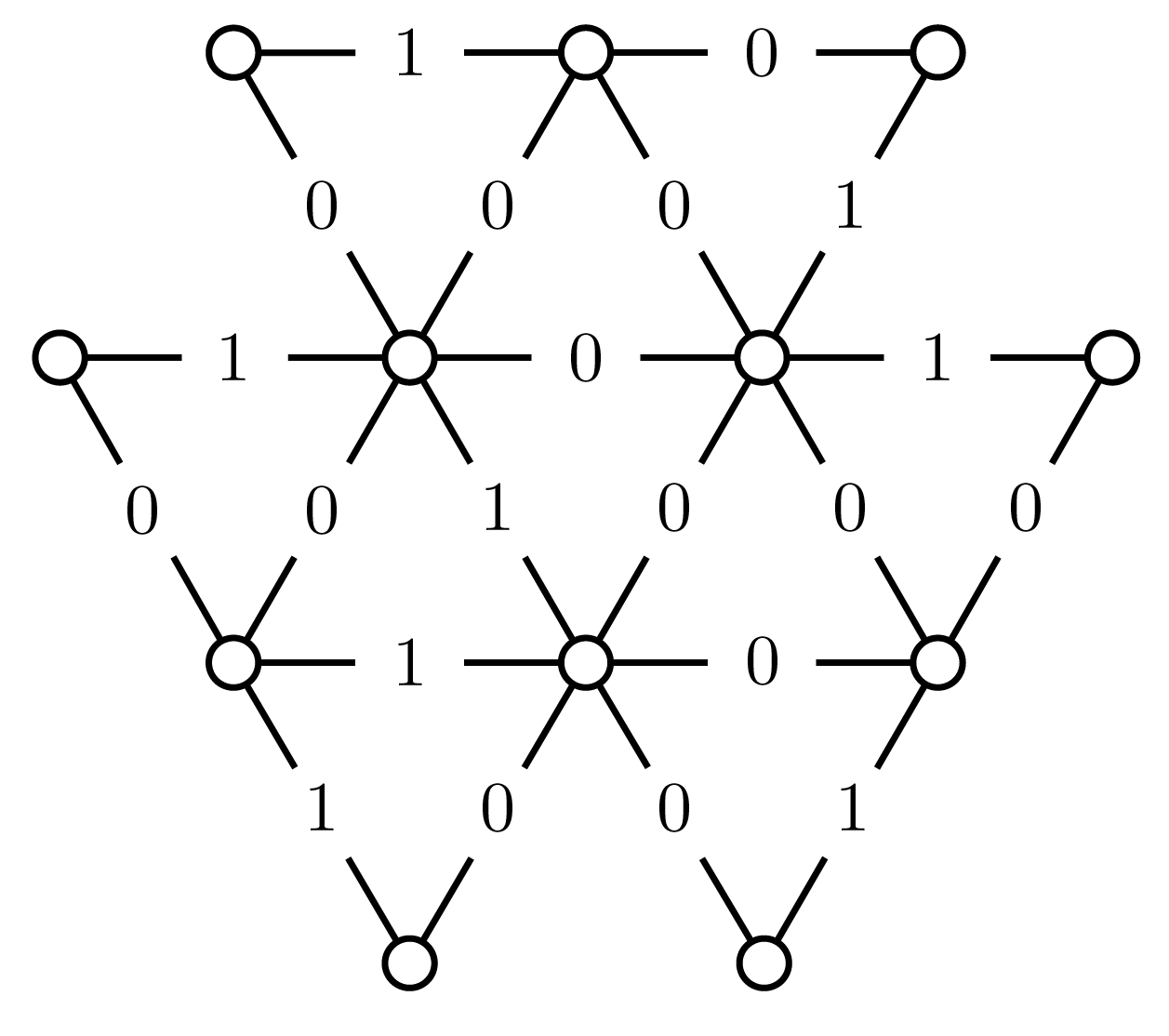
Note that every outer-planar graph is of treewidth $2$ and hence has inversion diameter at most $4$ by Lemma 1.2. We construct an outer-planar graph with inversion diameter $4$ verified by computer as Figure 1. The idea is to construct an outerplanar graph as “dense” as possible, and the labelling is searched by computer. The code is available on GitHub. Therefore, the upper bound $\operatorname{\mathrm{diam}}(\mathcal{I}(G))\leq 4$ for every outer-planar graph $G$ is tight.

4 Proof of Theorem 1.4

In this section, we intend to give the proof of Theorem 1.4.

From the definition, if $\operatorname{\mathrm{diam}}(\mathcal{I}(G))=k$, then for every graph $G^{\prime}$ obtained by removing a vertex from $G$, we have $\operatorname{\mathrm{diam}}(\mathcal{I}(G^{\prime}))\geq k-1$. In other words, removing one vertex can decrease the inversion diameter by at most $1$. Let $G$ be a graph. We say $G$ is $4$-diameter-critical if $\operatorname{\mathrm{diam}}(\mathcal{I}(G))=4$ and for every proper subgraph $G^{\prime}$, $\operatorname{\mathrm{diam}}(\mathcal{I}(G^{\prime}))\leq 3$. Clearly, a $4$-diameter-critical graph is connected. If $G$ is $4$-diameter-critical, by Proposition 2.1, there exists a labelling $\pi$ such that there is no $3$-dim vector assignment of $G$ respecting $\pi$. We call such a labelling $\pi$ a bad labelling.

Let $G$ be a $4$-diameter-critical graph respecting a bad labelling $\pi$ and $H$ a non-empty induced subgraph of $G$. Denote by $N_{G}(H)=\{v\in V(G)-V(H)\mid\exists u\in V(H),uv\in E(G)\}$ the neighbors of $H$ in $G-H$. By the definition of a $4$-diameter-critical graph, $G-H$ admits a $3$-dim vector assignment $f:V(G-H)\rightarrow\mathbb{F}_{2}^{3}$ respecting $\pi|_{G-H}$. For a vertex $v\in N_{G}(H)$, define $\mathcal{A}_{H,f}(v)=\{\mathbf{v}\in\mathbb{F}_{2}^{3}\mid\mathbf{v}\cdot f(u)=\pi(uv),\text{~for every~}uv\in E(G-H)\}$. Note that $f(v)\in\mathcal{A}_{H,f}(v)$. Here $\mathcal{A}_{H,f}(v)$ is the set of all possible vectors that can be assigned to $v$ while keeping the vector assignment valid on $G-H$.

Let $H$ be a fixed induced subgraph of $G$ and $f$ a fixed $3$-dim vector assignment of $G-H$ respecting $\pi|_{G-H}$. An available boundary family is a family of sets ${(\mathcal{B}_{f}(v))}_{v\in N_{G}(H)}$ satisfying the following properties.

1. $f(v)\in\mathcal{B}_{f}(v)\subseteq\mathcal{A}_{H,f}(v)$, and

2. $\{v\in N_{G}(H)\mid|\mathcal{B}_{f}(v)|\geq 2\}$ is an independent set in $G-H$.

When there is no ambiguity, we may ignore the subscript $f$ in $\mathcal{B}_{f}$.

The following lemma states that if we already have a vector assignment of $G-H$, then we can reassign the vectors $v\in N_{G}(H)$ using an available boundary family and the result is also a valid vector assignment.

Lemma 4.1

Let $H$ be an induced subgraph of a $4$-diameter-critical graph $G$ respecting a bad labelling $\pi$. Let $f$ be a $3$-dim vector assignment of $G-H$ with $\pi|_{G-H}$ and ${(\mathcal{B}_{f}(v))}_{v\in N_{G}(H)}$ an available boundary family. Then every $3$-dim vector assignment $g$ of $G-H$ satisfying

1. $g(v)=f(v)$, $\forall v\in V(G-H)-N_{G}(H)$, and

2. $g(v)\in\mathcal{B}_{f}(v)$, $\forall v\in N_{G}(H)$,

is a $3$-dim vector assignment of $G-H$ with $\pi|_{G-H}$.

Proof. We only need to verify that $g(v)\cdot g(u)=\pi(uv)$ for all $uv\in E(G-H)$. Note that $A\coloneqq\{v\in V(G-H)\mid g(v)\neq f(v)\}\subseteq\{v\in N_{G}(H)\mid|\mathcal{B}_{f}(v)|\geq 2\}$ from the definition. Then $\{v\in V(G-H)\mid g(v)\neq f(v)\}$ is an independent set. Since we already have $f(v)\cdot f(u)=\pi(uv)$ for all $uv\in E(G-H)$ and $\{v\in V(G-H)\mid g(v)\neq f(v)\}$ is an independent set, we now only need to verify that $g(v)\cdot g(u)=\pi(uv)$ for all $uv\in E(G-H)$ satisfying $u\in A$ and $v\notin A$. Since $g(u)\in\mathcal{B}_{f}(u)$ and $g(v)=f(v)$, we have $g(v)\cdot g(u)=\pi(uv)$ by the definition of $\mathcal{B}_{f}(u)$. $\square$

We say that $H$ is reducible respecting the labelling $\pi$ if there exists a $3$-dim vector assignment $f$ of $G-H$ respecting $\pi|_{G-H}$, and an available boundary family ${(\mathcal{B}_{f}(v))}_{v\in N_{G}(H)}$ and a $3$-dim vector assignment $g$ on $G[V(H)\cup N_{G}(H)]$ with $\pi|_{G[V(H)\cup N_{G}(H)]}$ such that $g(v)\in\mathcal{B}_{f}(v)$ for every $v\in N_{G}(H)$. The following lemma states that there is no reducible subgraph of a $4$-diameter-critical graph.

Lemma 4.2

Let $G$ be a $4$-diameter-critical graph respecting a bad labelling $\pi$. Then there is no reducible induced subgraph of $G$.

Proof. Suppose $H$ is an induced reducible subgraph of $G$. Then $G-H$ admits a $3$-dim vector assignment $f$ respecting the labelling $\pi|_{G-H}$, an available boundary family ${(\mathcal{B}_{f}(v))}_{v\in N_{G}(H)}$ and a $3$-dim vector assignment $g$ on $G[V(H)\cup N_{G}(H)]$ such that $g(v)\in\mathcal{B}_{f}(v)$ for every $v\in N_{G}(H)$. Define a function $h:V(G)\rightarrow\mathbb{F}_{2}^{3}$ by letting $h(v)=f(v)$ for every $v\in V(G-H)-N_{G}(H)$ and $h(v)=g(v)$ for every $v\in N_{G}(H)\cup V(H)$. By the definition, $h|_{G[V(H)\cup N_{G}(H)]}$ is a $3$-dim vector assignment respecting the labelling $\pi|_{G[V(H)\cup N_{G}(H)]}$. By Lemma 4.1, $h|_{G-H}$ is a $3$-dim vector assignment of $G-H$ respecting the labelling $\pi|_{G-H}$. Since there is no edge between $V(G-H)-N_{G}(H)$ and $V(H)$, $h$ is a $3$-dim vector assignment of $G$ with $\pi$, a contradiction. $\square$

In the following, we are going to find certain reducible structures in $4$-diameter-critical graphs.

Lemma 4.3

Let $G$ be a $4$-diameter-critical graph respecting a bad labelling $\pi$. For every vertex $v\in V(G)$, at least one edge adjacent to $v$ is labelled $1$ by $\pi$.

Proof. Suppose there exists a vertex $v\in V(G)$ such that $\pi(uv)=0$ for all $u\in N_{G}(v)$. Let $G^{\prime}=G-v$. Then $G^{\prime}$ admits a $3$-dim vector assignment $f$ with $\pi|_{G^{\prime}}$. Let $f(v)=\mathbf{0}\in\mathbb{F}_{2}^{3}$. Then it is not difficult to verify that $f$ is a $3$-dim vector assignment of $G$ with $\pi$, a contradiction. $\square$

Lemma 4.4

Let $G$ be a graph respecting a labelling $\pi$. If $G$ admits a $3$-dim vector assignment with $\pi$, then there exists a $3$-dim vector assignment $f$ with $\pi$ such that $f(v)\neq\mathbf{0}$ for every vertex $v\in V(G)$ of degree at most $2$.

Proof. Let $f$ be the $3$-dim vector assignment of $G$ with $\pi$ which minimizes $n_{f}=|\{v\in V(G)\mid f(v)=\mathbf{0},d_{G}(v)\leq 2\}|$. Suppose otherwise $n_{f}>0$. Let $w\in\{v\in V(G)\mid f(v)=\mathbf{0},d_{G}(v)\leq 2\}$ and $\mathcal{F}(w)=\{\mathbf{w}\in\mathbb{F}_{2}^{3}\mid\mathbf{w\cdot}f(u)=\pi(uw),\forall uw\in E(G)\}$. Then $|\mathcal{F}(w)|\geq 2$ since $d_{G}(w)\leq 2$. Choose $\mathbf{w}\in\mathcal{F}(w)-\{\mathbf{0}\}$ and define a function $g:V(G)\rightarrow\mathbb{F}_{2}^{3}$ by letting $g(v)=f(v)$ for every $v\in V(G)-\{w\}$ and $g(w)=\mathbf{w}$. It is easy to verify that $g$ is a $3$-dim vector assignment of $G$ with $\pi$, but $n_{g}<n_{f}$, a contradiction. $\square$

Lemma 4.5

Let $G$ be a $4$-diameter-critical graph of maximum degree $3$ respecting a bad labelling $\pi$. Then $G$ is 3-regular.

Proof. Suppose there exists a vertex $v\in V(G)$ such that $d(v)=1$. Let $uv\in E(G)$. Then by Lemma 4.3, $\pi(uv)=1$. Let $V(H)=\{v\}$. Then $N_{G}(H)=\{u\}$. By hypothesis, $G-v$ admits a $3$-dim vector assignment $f$ with $\pi|_{G-v}$. Since $d_{G-v}(u)\leq 2$, $|\mathcal{A}_{H,f}(u)|\geq 2$. Let $\mathcal{B}_{f}(u)=\mathcal{A}_{H,f}(u)$. Then ${(\mathcal{B}_{f}(u))}_{u\in N_{G}(H)}$ is an available boundary family. Let $g(u)\in\mathcal{B}(u)-\{\mathbf{0}\}$. We can choose $g(v)\in\mathbb{F}_{2}^{3}$ such that $g(v)\cdot g(u)=1$. Then $H$ is reducible, a contradiction with Lemma 4.2.

Suppose there exists a vertex $v\in V(G)$ such that $d(v)=2$. Let $N_{H}(v)=\{u_{1},u_{2}\}$. By Lemma 4.3, without loss of generality, assume $\pi(vu_{1})=1$. Let $V(H)=\{v\}$. Then $N_{G}(H)=\{u_{1},u_{2}\}$. By hypothesis and Lemma 4.4, $G-v$ admits a $3$-dim vector assignment $f$ with $\pi|_{G-v}$ such that $f(u_{1}),f(u_{2})\neq\mathbf{0}$. Let $\mathcal{B}(u_{1})=\{f(u_{1})\}$ and $\mathcal{B}(u_{2})=\mathcal{A}_{H,f}(u_{2})$. Then ${(\mathcal{B}(u_{i}))}_{i=1,2}$ is an available boundary family. Since $d_{G-v}(u_{2})\leq 2$, we have $|\mathcal{B}(u_{2})|\geq 2$. Let $g(u_{1})=f(u_{1})$. If $\pi(vu_{2})=1$ (resp. $\pi(vu_{2})=0$), choose $g(u_{2})\in\mathcal{B}(u_{2})-\{\mathbf{0}\}$ (resp. $g(u_{2})\in\mathcal{B}(u_{2})-\{f(u_{1})\}$). It is easy to verify in either case that there exists $g(v)\in\mathbb{F}_{2}^{3}$ such that $g(v)\cdot g(u_{i})=\pi(vu_{i})$ for $i=1,2$, so $H$ is reducible, a contradiction with Lemma 4.2. $\square$

Figure 2: $K_{4}^{-}$ in $G$.

Figure 3: Triangle in $G$.

Lemma 4.6

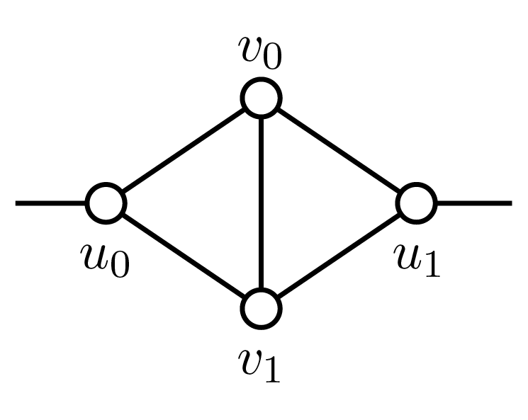
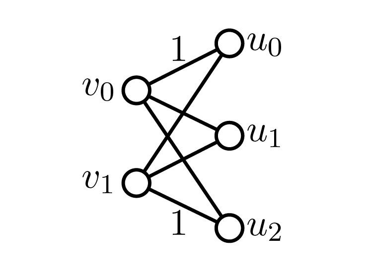
Let $G$ be a $4$-diameter-critical 3-regular graph respecting a bad labelling $\pi$. There is no induced $K_{4}^{-}$ in $G$, where $K_{4}^{-}$ is the graph obtained by deleting an edge in $K_{4}$.

Proof. Suppose there exists a $K_{4}^{-}$ in $G$ with vertex set $\{v_{0},v_{1},u_{0},u_{1}\}$ and $u_{0}u_{1}\notin E(G)$ (see Figure 3).

Let $H=G[\{v_{0},v_{1}\}]$. Then $N_{G}(H)=\{u_{0},u_{1}\}$. By hypothesis and Lemma 4.4, $G-H$ admits a $3$-dim vector assignment $f$ with $\pi|_{G-H}$ such that $f(u_{0}),f(u_{1})\neq\mathbf{0}$. Let $\mathcal{B}(u_{i})=\mathcal{A}_{H,f}(u_{i})$ for $i=0,1$. Then ${(\mathcal{B}(u_{i}))}_{i=0,1}$ is an available boundary family. We have the following properties:

1. For each $i\in\{0,1\}$, $|\mathcal{B}(u_{i})|\geq 4$ as $d_{G-H}(u_{i})=1$.

2. For each $i\in\{0,1\}$, if $\pi(v_{0}u_{i})=\pi(v_{1}u_{i})=0$, then $\mathbf{0}\notin\mathcal{B}(u_{i})$ by Lemma 4.3.

3. For each $i\in\{0,1\}$, at least one edge in $\{v_{0}v_{1},v_{i}u_{0},v_{i}u_{1}\}$ is labelled one by Lemma 4.3.

With the above properties, we claim that $H$ is reducible. The claim is proved by using a computer to enumerate all available boundary families with above properties. The source codes can be found on GitHub. From this, we derive a contradiction with Lemma 4.2. $\square$

Lemma 4.7

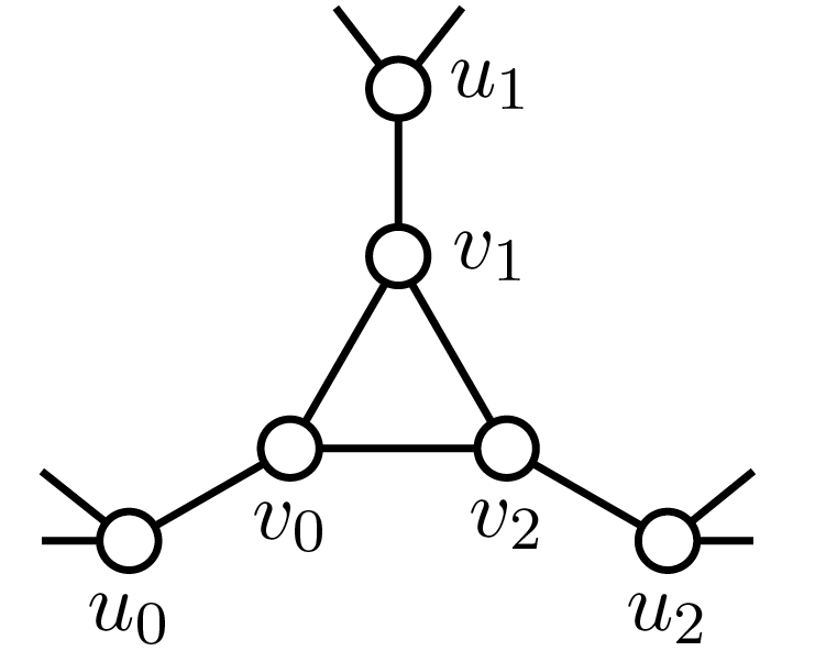
Let $G$ be a $4$-diameter-critical 3-regular graph respecting a bad labelling $\pi$. Then there is no triangle in $G$.

Proof. Suppose there exists a triangle with vertices $\{v_{0},v_{1},v_{2}\}$ and, for $i=0,1,2$, let $u_{i}$ be the neighbor of $v_{i}$ (see Figure 3). By Lemma 4.6, $u_{0},u_{1},u_{2}$ are either distinct vertices, or $u_{0}=u_{1}=u_{2}$. If $u_{0}=u_{1}=u_{2}$, then $G=K_{4}$ by $G$ being 3-regular. However, it was shown in [5] that $\operatorname{\mathrm{diam}}(\mathcal{I}(K_{4}))=3$, which contradicts the fact that $G$ is $4$-diameter-critical. Hence, we conclude that $u_{0},u_{1},u_{2}$ are distinct vertices. Let $V(H)=\{v_{0},v_{1},v_{2}\}$. Then $N_{G}(H)=\{u_{0},u_{1},u_{2}\}$. By hypothesis and Lemma 4.4, $G-H$ admits a $3$-dim vector assignment $f$ with $\pi|_{G-H}$ such that $f(u_{i})\neq\mathbf{0},i=0,1,2$. By relabelling as necessary, we can assume that $u_{0}$ satisfies the property: if $f(u_{1})=f(u_{2})$, then $f(u_{0})=f(u_{1})=f(u_{2})$. Let $\mathcal{B}(u_{0})=\mathcal{A}_{H,f}(u_{0})$ and $\mathcal{B}(u_{i})=\{f(u_{i})\},i=1,2$. Now we have the following properties:

1. $|\mathcal{B}(u_{0})|\geq 2$ as $d_{G-H}(u_{0})=2$.

2. For each $i=0,1,2$, at least one edge adjacent to $v_{i}$ is labelled one by Lemma 4.3.

3. If $\pi(u_{0}v_{0})=0$, then $\mathbf{0}\notin\mathcal{B}(u_{0})$, also by Lemma 4.3.

4. If $f(u_{1})=f(u_{2})$, then $f(u_{1})=f(u_{0})\in\mathcal{B}(u_{0})$.

With the above properties, we claim that $H$ is reducible, which is again proved with the help of a computer. The source code can be found on GitHub. Therefore, we derive a contradiction with Lemma 4.2. $\square$

Figure 4: $P_{3}$ with edges labelled one in $G$.

Figure 5: $K_{2,3}$ in $G$.

Lemma 4.8

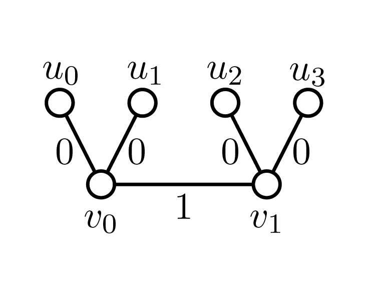
Let $G$ be a $4$-diameter-critical 3-regular graph respecting a bad labelling $\pi$. Then there is no $P_{3}$ with two edges labelled one in $G$.

Proof. Suppose there exists a path $wu_{0}u^{\prime}$ such that $\pi(wu_{0})=\pi(u_{0}u^{\prime})=1$. By Lemma 4.7, $u^{\prime}w\notin E(G)$. Let $u_{1},u_{2}$ be the neighbors of $w$ (see Figure 5). By Lemma 4.7, $\{u_{0},u_{1},u_{2}\}$ is an independent set. Let $V(H)=\{w\}$. Then $N_{G}(H)=\{u_{0},u_{1},u_{2}\}$. By hypothesis, $G-H$ admits a $3$-dim vector assignment $f$ with $\pi|_{G-H}$. Let $\mathcal{B}(u_{i})=\mathcal{A}_{H,f}(u_{i}),i=0,1,2$. Then ${(\mathcal{B}(u_{i}))}_{i=0,1,2}$ is an available boundary family. We have the following properties:

1. For each $i\in\{0,1,2\}$, $|\mathcal{B}(u_{i})|\geq 2$ as $d_{G-H}(u_{i})=2$.

2. $\mathbf{0}\notin\mathcal{B}(u_{0})$, because $\pi(u_{0}u^{\prime})=1$.

3. For each $i=1,2$, if $\pi(wu_{i})=0$, then $\mathbf{0}\notin\mathcal{B}(u_{i})$ by Lemma 4.3.

With the above properties, we claim that $H$ is reducible which is checked using a computer (GitHub). From this, we derive a contradiction with Lemma 4.2. $\square$

Lemma 4.9

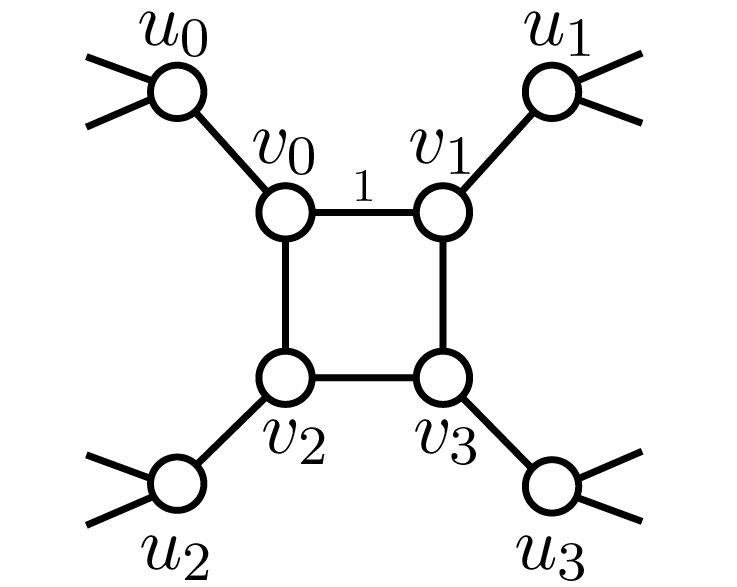
Let $G$ be a $4$-diameter-critical 3-regular graph respecting a bad labelling $\pi$. Then there is no $K_{2,3}$ in $G$.

Proof. Suppose there exists a $K_{2,3}$ with vertices ${\{v_{i}\}}_{i=0,1}\cup{\{u_{i}\}}_{i=0,1,2}$ and $u_{i}v_{j}\in E(G)$ for every $i=0,1$ and $j=0,1,2$ (see Figure 5). By Lemmas 4.3 and 4.8, without loss of generality, we can assume $\pi(v_{0}u_{0})=\pi(v_{1}u_{2})=1$ and other edges in $K_{2,3}$ are labelled zero. By Lemma 4.7, ${\{u_{i}\}}_{i=0,1,2}$ is an independent set. Let $H=G[\{v_{0},v_{1}\}]$. Then $N_{G}(H)=\{u_{0},u_{1},u_{2}\}$. By hypothesis, $G-H$ admits a $3$-dim vector assignment $f$. Let $\mathcal{B}(u_{i})=\mathcal{A}_{H,f}(u_{i}),i=0,1,2$. Then ${(\mathcal{B}(u_{i}))}_{i=0,1,2}$ is an available boundary family. We have the following properties:

1. For each $i\in\{0,1,2\}$, $|\mathcal{B}(u_{i})|\geq 4$ as $d_{G-H}(u_{i})=1$.

2. By Lemma 4.3, $\mathbf{0}\notin\mathcal{B}(u_{1})$ and $\mathbf{0}\in\mathcal{B}(u_{i})$ for $i=0,2$.

With the above properties, we claim that $H$ is reducible which is checked using a computer (GitHub). From this, we derive a contradiction with Lemma 4.2. $\square$

Figure 6: $C_{4}$ with at least one edge labelled one in $G$.

Figure 7: Edge labelled one in $G$.

Lemma 4.10

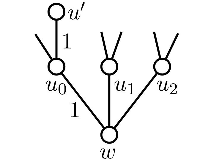
Let $G$ be a $4$-diameter-critical 3-regular graph respecting a bad labelling $\pi$. Then there is no $C_{4}$ with at least one edge labelled one in $G$.

Proof. Suppose there exists a copy of $C_{4}$ with vertices ${\{v_{i}\}}_{i=0,1,2,3}$ and with $\pi(v_{0}v_{1})=1$. Let $u_{i}$ be the neighbor of $v_{i}$ for $i=0,1,2,3$ (see Figure 7). By Lemmas 4.7 and 4.9, ${\{u_{i}\}}_{i=0,1,2,3}$ are distinct vertices. By Lemma 4.8, $\pi(v_{0}v_{2})=\pi(v_{1}v_{3})=0$. Let $H=C_{4}$. Then $N_{G}(H)=\{u_{0},u_{1},u_{2},u_{3}\}$. By hypothesis and Lemma 4.4, $G-H$ admits a $3$-dim vector assignment $f$ with $\pi|_{G-H}$ such that $f(u_{i})\neq\mathbf{0},i=0,1,2,3$.

Let us first consider the case $\pi(v_{2}v_{3})=0$. In this case, let $\mathcal{B}(u_{i})=\{f(u_{i})\},i=0,1,2,3$. Then ${(\mathcal{B}(u_{i}))}_{i=0,1,2,3}$ is an available boundary family. We claim $H$ is reducible with ${(\mathcal{B}(u_{i}))}_{i=0,1,2,3}$, which is proved by computer search (GitHub), and gives a contradiction with Lemma 4.2.

Now suppose $\pi(v_{2}v_{3})=1$. Then $\pi(v_{i}u_{i})=0,i=0,1,2,3$ by Lemma 4.8. Since $G$ is 3-regular, there exists $t\in\{1,2,3\}$ such that $u_{0}u_{t}\notin E(G)$. Let $\mathcal{B}(u_{i})=\mathcal{A}_{H,f}(u_{i})$ for $i=0,t$ and $\mathcal{B}(u_{i})=\{f(u_{i})\}$ for other $i$. Then ${(\mathcal{B}(u_{i}))}_{i=0,1,2,3}$ is an available boundary family. Since $\pi(v_{i}u_{i})=0$ for each $i$, we have $\mathbf{0}\notin\mathcal{B}(u_{i})$ by Lemma 4.3. Moreover, for $i=0,t$, we have $|\mathcal{B}(u_{i})|\geq 2$ since $d_{G-H}(u_{i})=2$. We claim that we can choose $\mathbf{u}_{i}\in\mathcal{B}(u_{i})$ for every $i\in\{0,1,2,3\}$ such that $\mathbf{u}_{j_{0}}=\mathbf{u}_{j_{1}}$ and $\mathbf{u}_{j_{2}}=\mathbf{u}_{j_{3}}$ do not occur, where $\{j_{0},j_{1},j_{2},j_{3}\}=\{0,1,2,3\}$. The claim can be proved easily.

Define $g:V(G-H)\rightarrow\mathbb{F}_{2}^{3}$ by letting $g(u_{i})=\mathbf{u}_{i},i=0,1,2,3$ and $g(v)=f(v)$ for all other vertices $v$. By Lemma 4.1, $g$ is a $3$-dim vector assignment of $G-H$ with $\pi|_{G-H}$.

Let $\mathcal{B}_{g}(u_{i})=g(u_{i}),i=0,1,2,3$, then ${(\mathcal{B}_{g}(u_{i}))}_{i=0,1,2,3}$ is an available boundary family. We claim $H$ is reducible with ${(\mathcal{B}_{g}(u_{i}))}_{i=0,1,2,3}$, which is proved by computer search (GitHub), and gives a contradiction. $\square$

Now we have plenty of forbidden structures in $G$, and we can finally prove Theorem 1.4.

Proof of Theorem 1.4. By contradiction. Let $G$ be a counterexample with the minimum number of vertices and, amongst all such examples, the minimum number of edges. Then $G$ is $4$-diameter-critical. Let $\pi$ be a bad labelling of $G$. Since $\Delta(G)\leq 3$, $G$ is 3-regular by Lemma 4.5.

By Lemma 4.3, at least one edge is labelled one in $G$. Pick an edge $v_{0}v_{1}\in E(G)$ labelled one. Let $u_{0},u_{1}$ be the neighbors of $v_{0}$ and $u_{2},u_{3}$ be the neighbors of $v_{1}$ (see Figure 7). By Lemmas 4.7 and 4.10, ${\{u_{i}\}}_{i=0,1,2,3}$ is an independent set. Let $H=G[\{v_{0},v_{1}\}]$. Then $N_{G}(H)=\{u_{0},u_{1},u_{2},u_{3}\}$. By hypothesis, $G-H$ admits a $3$-dim vector assignment $f$. Let $\mathcal{B}(u_{i})=\mathcal{A}_{H,f}(u_{i})$ for $i=0,1,2,3$. Then ${(\mathcal{B}(u_{i}))}_{i=0,1,2,3}$ is an available boundary family. Since $d_{G-H}(u_{i})=2$ for all $i=0,1,2,3$, we have $|\mathcal{B}(u_{i})|\geq 2$ for all $i=0,1,2,3$. By Lemma 4.3, at least one edge adjacent to $u_{i}$ is labelled one for every $i=0,1,2,3$. We know $v_{0}u_{0},v_{0}u_{1},v_{1}u_{2},v_{1}u_{3}$ are labelled zero. Thus, there is at least one edge adjacent to each $u_{i}$ in $G-H$ labelled one. Then by definition, $\mathbf{0}\notin\mathcal{B}(u_{i})$ for every $i=0,1,2,3$. Then we claim that $H$ is reducible, which is proved using a computer by enumerating all possibilities for $\mathcal{B}(u_{i})$ for each $i=1,2,3,4$ (GitHub), and gives a contradiction with Lemma 4.2. $\square$

References

- [1] N. Alon, E. Powierski, M. Savery, A. Scott, and E. Wilmer. Invertibility of digraphs and tournaments. SIAM Journal on Discrete Mathematics, 38(1):327–347, 2024.
- [2] G. Aubian, F. Havet, F. Hörsch, F. Klingelhoefer, N. Nisse, C. Rambaud, and Q. Vermande. Problems, proofs, and disproofs on the inversion number. The Electronic Journal of Combinatorics, 32(1), 2025.
- [3] J. Bang-Jensen, J. C. F. da Silva, and F. Havet. On the inversion number of oriented graphs. Discrete Mathematics & Theoretical Computer Science, 23(Special issues), 2022.
- [4] H. Belkhechine, M. Bouaziz, I. Boudabbous, and M. Pouzet. Inversion dans les tournois. Comptes Rendus. Mathématique, 348(13-14):703–707, 2010.
- [5] F. Havet, F. Hörsch, and C. Rambaud. Diameter of the inversion graph. arXiv preprint arXiv:2405.04119, 2024.
- [6] P. Scheffler. Die Baumweite von Graphen als ein Maß für die Kompliziertheit algorithmischer Probleme, volume 4. Akademie der Wissenschaften der DDR, Karl-Weierstrass-Institut für Mathematik, 1989.
- [7] J. van Leeuwen. Graph algorithms. In Algorithms and complexity, pages 525–631. Elsevier, 1990.