Loki: Low-rank Keys for Efficient Sparse Attention

Abstract

Inference on large language models (LLMs) can be expensive in terms of the compute and memory costs involved, especially when long sequence lengths are used. In particular, the self-attention mechanism used in LLM inference contributes significantly to these costs, which has sparked an interest in approximating the self-attention computation to reduce such costs. In this work, we propose to approximate self-attention by focusing on the dimensionality of key vectors computed in the attention block. Our analysis reveals that key vectors lie in a significantly lower-dimensional space, consistently across several datasets and models. Exploiting this observation, we propose Loki , a novel sparse attention method that ranks and selects tokens in the KV-cache based on attention scores computed in low-dimensional space. Our evaluations show that Loki is able to speed up the attention computation due to reduced data movement (load/store) and compute costs while maintaining the efficacy of the models better than other popular approximation methods.

1 Introduction

As large language models (LLMs) grow in size, deploying them for efficient inference presents substantial challenges, largely due to computation and memory access bottlenecks in the self-attention block [32], especially when handling long sequences. These challenges stem from the autoregressive nature of attention, which generates the output one token at a time. At each step, the entire preceding state, stored in the key-value (KV) cache, must be fetched from memory, which can sometimes exceed the size of the model parameters itself [18]. This frequent KV-cache access from GPU DRAM to registers becomes costly, as it scales quadratically with the output sequence length. In addition, matrix multiplications in the attention layers also have a quadratic scaling cost with sequence length, compounding the overall computational burden.

Several strategies [39, 26, 20] have been proposed to address this challenge by reducing the computational complexity and/or memory demands associated with the self-attention mechanism. One promising category of approaches focuses on approximating attention, employing techniques such as quantization or using a subset of the tokens in the KV-cache [11] (sparse attention).

In contrast to other sparse attention approaches that either permanently prune tokens from the key-value cache [39] or impose a fixed sparsity pattern [35], our proposed method dynamically selects key tokens at each generation step based on approximate attention scores and avoids deletions. This approach is inspired by a critical observation: across a range of LLMs and datasets, key tensors consistently occupy a significantly lower-dimensional space than the full attention head dimension. For instance, in Figure 1 (left), we show that across various LLMs [8, 16], 90% of the variance explained by PCA is captured at an effective key vector rank of around 80, despite the key tensor dimension being much larger (128).

Based on this observation, we introduce Loki, a sparse attention method that leverages the low-dimensional structure of key vectors to reduce data movement and computation costs without significantly impacting model quality. First, we apply PCA to keys generated from a calibration dataset, storing all principal components but using only the top $d$ (25-50%) to compute approximate attention scores during inference. This dimensionality reduction, informed by our previous observation that key vectors have low effective rank, allows us to efficiently identify the top-$k$ (12.5-25%) most relevant tokens using the approximate scores. For these selected keys, we then revert to the full dimensionality to compute the final attention scores, ensuring both efficiency and accuracy. Figure 1 (right) illustrates our approach.

Our theoretical complexity analysis demonstrates that Loki can provide significant speedups in the attention step. However, actually realizing these gains requires an efficient implementation of our method to minimize data movement in the additional operations introduced on top of the original self attention algorithm. Thus, we implement optimized sparse matrix multiplication kernels for Loki in Triton, leading to a speedup of up to 45% over the standard HuggingFace Transformer’s [34] attention implementation (vanilla attention) for Llama2-13B. For this setting, the average degradation in model accuracy (measured across 6 different benchmarks and 8 different models) is only 6.8%.

Our contributions can be summarized as follows:

• Detailed analysis showing the intrinsic low-dimensionality of keys in self-attention, its variation across layers for different models, and consistency across different datasets.

• Loki: a sparse attention method that exploits the aforementioned low dimensionality of keys to make the attention computation faster without sacrificing model quality.

• Optimized kernels for efficient implementation of Loki in PyTorch.

• Evaluation of Loki  on multiple LLMs and downstream tasks, showing that it can achieve significant speedups with minimal degradation in model quality.

Figure 1: Rank at which 90% of the variance is explained, averaged across all layers and heads for different models. Full rank is represented by the black dashed line (left). Overview of Loki (right).

2 Background and Related Work

The attention mechanism [32] is at the core of the transformer architecture. Consider a single attention query head with head dimension $D$, processing an input token sequence of length $S$. During auto-regressive generation, the output of the attention head is calculated as:

$$\boldsymbol{y}=\mathrm{softmax}\Bigl(\dfrac{\mathbf{q}\mathbf{K}^{\top}}{\sqrt{D}}\Bigr)\cdot\boldsymbol{V}$$ (1)

where $\mathbf{q}\in\mathbb{R}^{1\times D}$ is the query, and $\mathbf{K}\in\mathbb{R}^{S\times D}$ and $\mathbf{V}\in\mathbb{R}^{S\times D}$ are the key and value caches respectively. Additionally, newer transformer models add Rotary Position Embeddings (RoPE) [29] to the keys and query, before computing the attention scores. Since every query attends to all past keys, the mechanism has a quadratic complexity $\mathcal{O}(S^{2})$ in number of input $+$ generated tokens.

2.1 Related Work

Numerous studies have explored the low-rank structures in transformers for various purposes. Linformer [33] demonstrated that the attention score matrix is low-rank and proposed alternative low-rank attention formulations during training for linear computational complexity. LoRA [13] showed that parameter updates to a transformer model during fine-tuning reside in a low-dimensional subspace. To the best of our knowledge, our work is the first to study the intrinsic low dimensionality of the attention keys themselves and demonstrate the generalizability of this low-dimensional structure across different models (for natural language data).

Sparse-transformers [5] was one of the first works to introduce a sparse-attention method employing strided sparsity patterns in the attention mechanism. Reformer [17] used locally-sensitive hashing to compute attention scores in a sparse manner. Performer [6] used positive orthogonal random features to approximate the attention mechanism. Unlike these methods, which require training or fine-tuning, our approach operates entirely post-training without any fine-tuning.

Another category of sparse attention methods employ token eviction policies to permanently delete tokens from the KV-cache based on some heuristic. StreamingLLM [35] uses initial tokens and a rolling KV-cache for processing infinite-length sequences. Zhang et al. [39] retain only "Heavy Hitters" tokens in the KV-cache based on accumulated attention scores. Scissorhands [20] prioritizes important tokens based on the "Persistence of Importance Hypothesis". Ge et al. [10] propose an adaptive eviction policy for each transformer layer. These methods are effective in reducing the memory and compute footprint of the attention but suffer from permanent loss of information leading to a non-trivial degradation in model quality. Our method does not involve any permanent loss of information with the trade-off of not reducing the memory footprint. Quantization-based approximate approaches [14, 23] are complementary to our work and can be applied in tandem.

SparQ Attention [26] is a recent work that inspires our approach. They use high-magnitude query dimensions and corresponding key dimensions for approximate attention scoring, followed by computing the full attention scores for the top-$k$ keys. However, their method requires costly non-contiguous column indexing of the key vectors. Further, they store two copies of the past keys for efficiency, increasing memory use by 50%. In contrast, Loki avoids the extra memory and leverages the natural ordering of principal components, allowing for a more efficient slicing operation.

A concurrent work, InfiniGen [19], accelerates attention by pre-fetching top-$k$ keys from CPU to GPU memory, using SVD-based low-rank approximation of the attention scores. While their low-rank approximation is similar to  Loki, our work provides deeper analysis of the intrinsic low-rank structure of attention keys and focuses on speeding up attention computation without CPU offloading. Importantly, their results affirm the benefits of the low-dimensional nature of attention keys applied in other contexts.

3 Dimensionality Analysis of Attention Keys

As noted in Section 1, Loki, our proposed method for sparse self-attention, is based on the observation that key tensors consistently reside in a lower-dimensional space than the full attention head dimension suggests. Here, we present empirical evidence supporting this claim by performing PCA on the keys generated in several language models and datasets.

3.1 Models and Datasets Used

To investigate the dimensionality of attention keys, we run 11 transformer-based models: Llama-2 7B/13B/70B [31], Llama-3 8B/70B [8], TinyLlama-1.1B [38], Pythia-6.9B [4], Mistral-7B [15], Mixtral-8x7B/8x22B [16], and Phi3-Mini-4K [22] on three popular English language datasets: WikiText-2 [21] (Validation Split), C4 [25] (Custom Split), and BookCorpus [40] (Custom Split). Custom splits are used for datasets where the validation split is not available. We run perplexity evaluation on these datasets and save the generated attention keys, before and after the application of rotary embeddings [29], referred to as pre-rotary and post-rotary keys, respectively throughout the paper. We then perform PCA on all the keys generated for each layer and head individually.

The metric we use in our analysis is the rank at which $v$% of the variance is explained by the principal components. We calculate this metric for each layer and head of the models as follows:

$$Rank_{l,h}@v=\min\left\{d\in\mathbb{Z}^{+}:\sum_{j=1}^{d}\lambda_{l,h}^{j}\geq v/100\right\}$$ (2)

where, $\lambda_{l,h}^{j}$ is the $j^{th}$ normalized eigenvalue of the covariance matrix of the keys for layer, $l$ and head, $h$. We average this metric ranks across all heads of layer, $l$ and refer to it as $Rank_{l}@v$.

3.2 Findings and Discussion

Figure 1 (left) shows the average $Rank_{l}@90$ across all layers for models with full key dimensionality of 128. We can see that the average rank is significantly lower than the full dimensionality of the keys for all models. Diving deeper, we present a layer-wise analysis for a few models: Llama2-7B, Llama3-70B, Mixtral-8x7B, and Phi3-Mini-4K in Figure 2. The results for the other models are similar and can be found in Appendix A.1.

Figure 2: Rank at which 90% of the variance is explained for pre-rotary and post-rotary keys produced by each layer averaged across all heads ($Rank_{l}@90$) for different models. We observe that all models exhibit significantly low rank (full dimensionality is 128 or 96 represented by the black dashed line) consistently across all datasets.

We observe that the dimensionality of the keys (both pre-rotary and post-rotary) is significantly lower than the full dimensionality of the keys across all calibration datasets. Furthermore, the $Rank_{l}@90$ for a particular layer is consistent across datasets, for all combinations of models and datasets. This indicates that the lower-dimensional structure of the keys is consistent when calculated using different calibration datasets. Another trend we observe is that the initial layers of most models have a very low rank, as compared to the later layers, and this trend is particularly prominent for the pre-rotary keys. Lastly, we also observe that for most models, the average of $Rank_{l}@90$ across all layers is lower for pre-rotary keys as compared to post-rotary keys, indicating that the rotary embeddings increase the dimensionality of the keys. Further analysis on the variation of the rank across different heads within a layer and across different layers within a model can be found in Appendix A.1.

These results indicate the existence of the following properties: (1) The keys produced by the attention layers of transformer models lie in a significantly lower-dimensional space. (2) The lower-dimensional structure of the keys is consistent across different calibration datasets. (3) Rotary embeddings increase the dimensionality of the keys for most models. We now use the first two properties to propose Loki, an efficient sparse-attention method.

4 Loki: Low-Dimensional Key Representations

We now describe our proposed algorithm for sparse attention – Loki. Loki leverages low dimensional projections of the keys in the KV-cache to efficiently and accurately select the top-$k$ (12.5-25%) most relevant tokens for self attention. Before discussing our approach, let us first look at some theoretical properties of attention in the PCA-transformed space of the key tensors.

4.1 Properties of Attention in the PCA-transformed Space

We begin by proving two lemmas that provide the rationale for our approach to compute attention in the PCA-transformed space.

Lemma 4.1.

Let $D$ be the dimension of an attention head and $\mathbf{P}\in\mathbb{R}^{D\times D}$ be the PCA projection matrix of key tensors calibrated offline on a dataset. Assuming we are generating the $S^{\mathit{th}}$ token in the sequence, let $\mathbf{q}_{S}\in\mathbb{R}^{1\times D}$ be the query vector for the $S^{th}$ token, $\mathbf{K}_{:S}\in\mathbb{R}^{S\times D}$ be the key vectors, including the past $(S-1)$ keys and the current key. Then, the attention scores computed using the PCA-transformed query and keys are equivalent to the attention scores computed using the original query and keys.

Proof.

Let $\mathbf{\hat{q}}_{S}=\mathbf{q}_{S}\mathbf{P}$ and $\mathbf{\hat{K}}_{:S}=\mathbf{K}_{:S}\mathbf{P}$ be the PCA transformed query and key vectors. Focusing on the dot product term in the attention computation (Equation 1), we have:

$$\mathbf{q}_{S}\mathbf{K}_{:S}^{T} =\mathbf{q}_{S}(\mathbf{\hat{K}}_{:S}\mathbf{P}^{T})^{T}\text{ [inverting the PCA transform]}$$

$$=\mathbf{q}_{S}((\mathbf{P}^{T})^{T}\mathbf{\hat{K}}_{:S}^{T})=(\mathbf{q}_{S}\mathbf{P})\mathbf{\hat{K}}_{:S}^{T}=\mathbf{\hat{q}}_{S}\mathbf{\hat{K}}_{:S}^{T}$$

It is important to note here that Lemma 4.1 holds for any orthogonal $\mathbf{P}$. ∎

Lemma 4.2.

Let $\mathbf{\hat{K}}_{:S,:d}\in\mathbb{R}^{S\times d}$ ($d<D$) be the reduced dimension key vectors obtained by projecting the key vectors onto the first $d$ principal components of $\mathbf{P}$ . Then, the attention scores computed using $\mathbf{\hat{K}}_{:S,:d}$ are a good approximation of the the actual attention scores.

Proof.

Let $\textbf{R}_{:d}\in\mathbb{R}^{d\times D}$ be an orthogonal transformation that transforms the keys into the reduced dimension space as $\mathbf{L}_{:S,:d}=\mathbf{K}_{:S}\textbf{R}_{:d}$. Our objective is to minimize the following expression:

$$\min_{\mathbf{R}_{:d}}||\mathbf{q}_{S}\mathbf{K}_{:S}^{T}-\mathbf{q}_{S}(\mathbf{L}_{:S,:d}\mathbf{R}_{:d}^{T})^{T}||_{2}^{2}$$ (3)

Using Cauchy-Schwarz inequality, we have:

$$||\mathbf{q}_{S}\mathbf{K}_{:S}^{T}-\mathbf{q}_{S}(\mathbf{L}_{:S,:d}\mathbf{R}_{:d}^{T})^{T}||_{2}^{2} \leq||\mathbf{q}_{S}||_{2}^{2}||\mathbf{K}_{:S}^{T}-(\mathbf{L}_{:S,:d}\mathbf{R}_{:d}^{T})^{T}||_{2}^{2}$$ (4)

We change our objective to minimize the upper bound in the RHS instead of the original objective. We know that PCA minimizes the reconstruction error (2nd term in the RHS) among all the orthogonal transformations. Thus, it follows that the optimal value of $\mathbf{R}^{*}_{:d}=\mathbf{P}_{:d}$, and $\mathbf{L}^{*}_{:S,:d}=\mathbf{\hat{K}}_{:S,:d}$ ∎

Since we minimize an upper bound when proving Lemma 4.2, it is possible that some other transformation might give a better approximation to the dot product. Thus, in our experiments, we use PCA transforms computed on both the pre-rotary and post-rotary keys as candidate transformations.

Based on these lemmas and the inherent low-dimensional nature of key tensors in attention, we now introduce the workings of the Loki algorithm.

4.2 PCA-based Top-K Algorithm

Loki implements a PCA-based Top-K Attention approach. Previous works have shown that attention scores for a query are highly concentrated on a small subset of keys [36, 30]. This observation has motivated several methods that compute attention using only the top-$k$ most relevant keys. However, these previous works either compute the exact attention scores and then select the top-$k$ keys [12] or compute non-exact scores but have significantly higher memory requirements [26]. Loki alleviates these issues by computing approximate attention scores (for ranking the keys) in the reduced lower-dimensional space, without any significant increase in memory requirements. Algorithm 1 shows our Loki method. Line 5 of the algorithm computes the approximate attention scores using $d$ principal dimensions of the query and key vectors. Lines 6-7 select the top-$k$ keys based on the approximate attention scores. Line 8 computes the exact attention scores using the selected top-$k$ keys, directly in the transformed space (Lemma 4.1).

Algorithm 1 Loki: PCA-based Top-K Attention

1: At the $S^{th}$ step - Input: $\mathbf{x}_{S}\in\mathbb{R}^{1\times D}$, KV-cache: $\mathbf{\hat{K}}_{:S-1},\mathbf{V}_{:S-1}\in\mathbb{R}^{(S-1)\times D}$, Projection Matrix: $\mathbf{P}\in\mathbb{R}^{D\times D}$, Configuration parameters (reduced dimensionality, top-$k$): $d$, $k$

2: function Loki-Attention($\mathbf{x}_{S},\mathbf{\hat{K}}_{:S-1},\mathbf{V}_{:S-1},\mathbf{P},d,k$)

3:   $\mathbf{q}_{S},\mathbf{k}_{S},\mathbf{v}_{S}\leftarrow computeQKV(\mathbf{x}_{S})$

4:   $\mathbf{\hat{q}}_{S}\leftarrow\mathbf{q}_{S}\mathbf{P}$, $\mathbf{\hat{k}}_{S}\leftarrow\mathbf{k}_{S}\mathbf{P}$

5:   $\mathbf{\hat{K}}_{:S}\leftarrow concat(\mathbf{\hat{K}}_{:S-1},\mathbf{\hat{k}}_{S})$, $\mathbf{V}_{:S}\leftarrow concat(\mathbf{V}_{:S-1},\mathbf{v}_{S})$

6:   $\mathbf{a}_{approx}\leftarrow\mathbf{\hat{q}}_{S,:d}(\mathbf{\hat{K}}_{:S,:d})^{T}$

7:   $indices\leftarrow topk(\mathbf{a}_{approx},k)$

8:   $\mathbf{\hat{K}}_{:S}^{\prime}\leftarrow\mathbf{\hat{K}}_{:S}[indices]$, $\mathbf{V}_{:S}^{\prime}\leftarrow\mathbf{V}_{:S}[indices]$

9:   $\mathbf{a}_{exact}\leftarrow softmax(\frac{\mathbf{\hat{q}}_{S}\mathbf{\hat{K}}_{:S}^{T}}{\sqrt{D}})$

10:   return $\mathbf{a}_{exact}\mathbf{V}_{:S}^{\prime}$

11: end function

Compute and Memory Analysis: For vanilla attention, the complexity of computing $\mathbf{q}_{S}\mathbf{K}_{:S}^{T}$ is $\mathcal{O}(DS)$ and the complexity of multiplying the values with the attention scores is $\mathcal{O}(DS)$. For Loki, the complexity of calculating the approximate attention scores (Line 5) is $\mathcal{O}(dS)$. The complexity of selecting the top-$k$ keys (Lines 6-7) is approximately $\mathcal{O}(Slog(S)+k)$ (sorting followed by selection). The complexity of calculating the exact attention scores and multiplying with the values (Line 8-9) is $\mathcal{O}(2Dk)$. Additionally, the complexity of projections into the PCA space (Line 3) is $\mathcal{O}(2D^{2})$. Assuming the complexity of selecting the top-$k$ keys is small compared to the other operations, the overall complexity of the algorithm is $\mathcal{O}(dS+2Dk+2D^{2})$. Then, we have:

$$speedup=\frac{2DS}{dS+2Dk+2D^{2}}=\frac{1}{d/2D+k/S+D/S}\approx\frac{1}{d_{f}/2+k_{f}}\hskip 10.00002pt(\text{given }D<<S)$$ (5)

where, $d_{f}=d/D$ and $k_{f}=k/S$. The memory requirement of the KV-cache is the same as the original attention, with a small overhead of storing the PCA transformation matrix.

4.3 Implementation in Triton

Performing Loki efficiently involves complex indexing operations within the KV-cache (lines 5 and 7 of Algorithm 1). Standard PyTorch operations create temporary, dense copies of the KV-cache data in memory, leading to slowdowns due to expensive memory access. To alleviate this issue, we develop optimized kernels in Triton [1] for the three matrix multiplication operations in Loki. Our kernels can directly access relevant subsets of the KV-cache (both feature and sequence dimensions) and perform computations within GPU registers. This eliminates the need for creating dense copies, significantly improving performance. Our approach builds on SparQ [26], which introduced similar kernels for top-$k$ attention calculations. However, we identified and addressed inefficiencies in the SparQ kernels, which resulted in speedups of nearly $2-3\times$ in certain scenarios. (see Appendix C).

5 Experimental Setup

We evaluate Loki on the basis of perplexity using the WikiText-2 [21] dataset (test split), and on the basis of downstream task performance for short contexts using the LM-harness benchmark [9] and long contexts using LongBench [2]. For the short-context evaluation, we choose the same tasks and associated metrics as the HuggingFace OpenLLM leaderboard [3]. For the LongBench tasks, we evaluate on all the English language tasks.

We compare our method against three methods – full attention without any approximations, the exact TopK approach which computes the exact attention scores and then uses the top-$k$ tokens to compute the final output, and H₂O [39], a popular token-eviction method. For these comparisons, we show the results with a budget size of $k_{f}$ = 0.25 and 0.125. For our method, we additionally use $d_{f}$ = 0.25 and 0.125. This configuration of our represents a 2.6x theoretical speedup. Table 1 provides an overview of the methods compared and the associated budget terms. H₂O’s budget was split equally between the heavy hitter and recent tokens, as per the author’s recommendations. For H₂O, we were unable to run the GSM8K task as the the author’s ML benchmarking code was too memory intensive to run for that task. For the aforementioned experiments, we generate PCA transforms using the WikiText-103 dataset. For the LongBench tasks, we compare our method with the full attention baseline as we were unable to run H₂O due to memory constraints.

For the generalizability study, we compare the results of our method with PCA transforms from different calibration datasets: WikiText-103 [21], C4 [25], and BookCorpus [40]. Additionally, we also benchmark our triton based implementation of Loki by running an attention microbenchmark on a Llama2-13B-like setup (same hidden size and number of heads) for various prompt and generation lengths, and demonstrate speedups over vanilla attention.

Table 1: Explanation of key-budget and dimensionality (Dim.) for different approaches, along with the expected speedup and memory savings.

Method Budget Dim. Description Speedup Memory Savings Exact Top-K $k_{f}$ Full $k_{f}$ fraction of keys selected using exact attention scores No No H₂O $k_{f}$ Full $k_{f}$ fraction of keys & values selected using H₂O policy $\frac{1}{k_{f}}$ $\frac{1}{k_{f}}$ Loki $k_{f}$ $d_{f}$ $k_{f}$ fraction of keys &values selected using attention scores computed with $d_{f}$ fraction of full dimensionality $\frac{1}{(d_{f}/2)+k_{f}}$ No

All experiments are run on NVIDIA A100 GPUs with 40 and 80 GB of memory on the Perlmutter [24] supercomputer. For larger models, we use AxoNN [27, 28] to shard the model across multiple GPUs.

6 Results

We now present the comparisons of Loki with full attention and other sparse attention methods, including a comparison of the computation times.

6.1 Comparison with Full Attention

Let us begin our discussion with Figure 3, showing the perplexity (left) and short-context downstream task evaluation (right) results for Loki on different models. We focus on the Llama2-7B model, comparing pre-rotary (light green/purple) and post-rotary (dark green/purple) PCA transforms for different $k_{f}$ and $d_{f}$ values. For Llama2-7B, we see that the performance of both candidate transforms is similar. This trend is consistent across all the models except for Llama3-8B/70B and Mistral-7B, where the post-rotary PCA transform performs significantly worse than the pre-rotary one. For Llama3-8B, perplexity jumps from about 5 for the full attention to over 10, a significant decline not seen with the pre-rotary transform. Mistral-7B shows a similar pattern. This is a surprising observation since attention scores are calculated from post-rotary keys in the original attention mechanism. A possible explanation is that post-rotary PCA captures token distributions tied to specific positions in the calibration dataset, while pre-rotary PCA may generalize better by using less positional information. Nevertheless, at least one of the PCA transformations performs well for every model. For subsequent results, we only show the better-performing transformation for each model.

Figure 3: Evaluation of Loki on perplexity (left plot) and short-context tasks (right plot) for different models. Task accuracy is an average across all short-context tasks mentioned in 5.

Figure 4 shows the performance of Loki on the LongBench tasks for the Llama2-7B-Chat model. We see that for all tasks, either one of the two candidate transforms performs similarly to full attention. For Summarization, Few Shot Learning, Synthetic, and Code Completion task categories, the best performing Loki configuration is at par or better than the full attention model. For the Single-Doc QA and Multi-Doc QA task categories,  Loki performs slightly worse than the full attention model, with the biggest drop in performance observed for HotpotQA of around 3%. Comparing different $(k_{f},d_{f})$ settings, we see that using $k_{f}$ = 0.25 and $d_{f}$ = 0.25 (green), is better than using $k_{f}$ = 0.125 and $d_{f}$ = 0.5 (purple) for all models and tasks (short-context and long-context). These two settings balance speed and performance well, with the first being superior for accuracy.

Figure 4: Evaluation of Loki on LongBench tasks for the Llama2-7B-Chat model.

6.2 Comparison with Other Sparse Attention Methods

Next, we compare the performance of Loki with other methods, using $k_{f}$ = 0.25 for all methods and $d_{f}$ = 0.25 for ours. Table 2 shows the perplexity results for Llama2-7B/13B, Llama3-8B, and Mistral-7B. Loki’s perplexity drop is within 0.1 of full attention across all models, a threshold considered acceptable for attention mechanism approximations [37]. In contrast, H₂O’s perplexity drop nears 0.2 for all models. Figure 5 confirms this trend on short-context evaluation. Loki performs similar to full attention for all models, except Llama3-8B, where the performance is notably worse, but still better than H₂O. Importantly, on the challenging MMLU task, Loki degrades less than H₂O.

Table 2: Perplexity evaluation of Loki and other approaches for different models (lower is better).

Method $k_{f}$ $d_{f}$ Speedup Llama2-7B Llama2-13B Llama3-8B Mistral-7B Full Attention - - No 5.1101 4.5680 5.5696 4.9140 Exact-TopK 0.25 - No 5.1809 4.5926 5.5716 4.9171 H₂O 0.25 - Yes 5.2810 4.7009 5.7056 5.0805 Loki 0.25 0.25 Yes 5.2017 4.6102 5.6648 4.9233

Figure 5: Downstream task performance for Loki and other approaches for different models (higher is better). GSM8K is excluded, as we were unable to run H₂O for this task.

It is important to note here that Loki is designed to be compatible with other sparse attention methods. For instance, token-eviction methods like H₂O delete tokens to save KV-cache memory, whereas Loki reduces memory bandwidth by selecting the top-$k$ tokens without deletion, making them orthogonal. A combined approach could involve using H₂O to delete tokens, then applying Loki to select top-$k$ tokens from the remaining cache. Similarly, Loki is theoretically orthogonal to quantization methods.

Comparing Loki with Exact-TopK, we find similar performance for Llama2-7B/13B and Mistral-7B. Exact-TopK represents the upper performance bound for Loki if it could perfectly select the top-$k$ tokens. To understand why Loki works well, we examined the top-$k$ agreement between  Loki’s reduced dimensional attention scores and exact attention scores. Figure 6 shows the Jaccard similarity between the top-$k$ tokens selected by both methods across all layers and heads for Llama2-7B. For the settings: ($k_{f}=0.25$, $d_{f}=0.25$) and ($k_{f}=0.125$, $d_{f}=0.5$), evaluated in Figure 3, the Jaccard similarity is around 0.9, validating that the Loki is able to select the top-$k$ tokens with high accuracy.

Figure 6: Top-$k$ agreement between Loki and Exact-TopK methods for Llama2-7B (left plot). Performance of Loki using transformations derived from different calibration datasets (middle plots). Benchmarking vanilla attention and Loki for Llama2-13B using huggingface transformers with cache append times (right plot, prompt length = 3072, generation length = 512).

6.3 Generalizability

We now turn our attention to the generalizability of the PCA transformations used in our method. Figure 6 (middle) shows the performance of Loki using PCA transformations derived from different calibration datasets ($k_{f}=0.25,d_{f}=0.25$). We see that the performance of Loki is consistent across different calibration datasets, indicating that the PCA transformations used in our method are generalizable. This is an important observation as it shows that the PCA keys can be generated using a variety of calibration datasets and still achieve good performance.

6.4 Computational Efficiency

We now turn our attention to the computational efficiency of Loki. Analyzing Llama2-13B with Hugging Face Transformers exposed an interesting bottleneck (Figure 6, rightmost). Regardless of the attention type (vanilla or Loki), more than 80% of the time is consumed within the Hugging Face framework for appending key-value pairs of the latest token to the KV-cache. This shared bottleneck minimizes the overall performance improvement of our optimizations. We hypothesize that using a more advanced inference system like vLLM [18] could significantly reduce this append time, but leave that exploration for future work. To isolate the impact of our optimizations, the plots in Figure 7 focus solely on the attention computation time, excluding the KV-cache append time.

Figure 7: Time per layer for vanilla attention (V) and Loki (L-A: ${k_{f}=0.25,d_{f}=0.25}$; L-B: ${k_{f}=0.125,d_{f}=0.25}$) for Llama2-13B using huggingface transformers (left two plots). LongBench average accuracy for different Loki configurations, alongside micro-benchmark attention times (right plot, all layers, prompt length = 3500 & generation length = 512). We choose the prompt length to match LongBench’s configuration for this model and generation length to match the maximum in any LongBench task. For both figures, we use a batch size of 16 and report the average time over 10 trials (std. dev. in measured times was less than 0.05 percent of the mean).

In the left plot of Figure 7, we see that Loki speeds up the total attention compute time (excluding KV-cache appends) compared to vanilla attention across various prompt and generation lengths. For a prompt length of 3072 and generation length of 512, Loki achieves nearly a 45% speedup, despite the fact that it incurs an extra matrix multiplication operation. The breakdowns also show that the top-$k$ operation is nearly as expensive as the smaller matrix multiplications, which is a significant bottleneck. Replacing PyTorch’s top-$k$ with a custom kernel could improve this. For the shorter prompt length of 2048 we observe a speedup of around 40% (generation length = 512), slightly lower than the speedup at 3072. This trend is expected as larger prompts result in a bigger KV-cache, amplifying the impact of our optimizations.

Figure 7 (Right) shows the accuracy vs. attention time trade-off across various $k_{f},d_{f}$ settings of Loki, with accuracy measured on LongBench and attention times from our microbenchmark. The previously evaluated settings, $k_{f}=0.25,d_{f}=0.25$ and $k_{f}=0.125,d_{f}=0.5$, provide a good balance between performance and accuracy, with $k_{f}=0.25,d_{f}=0.25$ favoring accuracy slightly and $k_{f}=0.125,d_{f}=0.5$ favoring performance.

7 Conclusion

In conclusion, we introduced Loki, an algorithm for efficient sparse attention that does not compromise the model quality while reducing the computational complexity of self attention. We made a crucial observation that key vectors in attention lie in a low-dimensional space, across different models and datasets. Leveraging this insight, Loki uses attention scores computed in a lower-dimensional space to rank and select the top-$k$ most relevant tokens from the KV-cache. It then uses the full dimensionality only for the selected tokens to compute the final attention. Our theoretical analysis shows that Loki can provide significant speedups in the attention step. To implement this efficiently, we develop optimized kernels for the various sparse matrix multiplications in our approach. Our empirical evaluation shows that Loki performs better than popular approximation methods on a variety of models and tasks, with respect to preserving model quality. Finally, we show that Loki can provide speedups of up to 45% over the vanilla attention empirically, making it a promising approach to address the computational challenges in transformer inference.

Limitations and Future Work: Loki does not focus on reducing memory usage of the KV-cache currently. As mentioned previously in 6.2, it can potentially be combined with other sparse attention method for improved memory-performance-accuracy trade-offs. Another direction involves storing the KV-cache in CPU memory and transferring only the top-$k$ keys and values to the GPU [19].

While Loki outperforms vanilla attention in our benchmarks, practical deployment would require integration with efficient attention kernels like FlashAttention [7]. As seen in our compute benchmarking, the top-$k$ selection operation could introduce a bottleneck towards achieving this. Investigating this bottleneck and integrating Loki with optimized attention kernels is left for future work.

Our finding of the keys’ low intrinsic dimensionality suggests promising research directions. The variation of this dimensionality across heads and layers could further be explored. We briefly experimented with a variable $d_{f}$ policy per layer (see Appendix B.2), but did not observe significant significant improvements. A more sophisticated policy could be explored in future work.

Appendix

Appendix A Comprehensive Dimensionality Analysis

A.1 Complete Key-Dimensionaltiy Analysis for All Models

Figure 8: Rank at which 90% of the variance is explained for pre-rotary and post-rotary keys produced by each layer averaged across all heads ($Rank_{l}@90$) for different models. We observe that all models exhibit significantly low rank consistently across all datasets.

In this section, we present our extended dimensionality analysis results (from 3) for all the models we experimented with. Figure 8 displays the $Rank_{l}@90$ values for all models referenced in Section 3. Our analysis reveals that the low dimensionality of the keys is consistently observed across all models and datasets. Results for all models resemble those shown in Figure 2 of the main text. The models we tested cover a wide range of sizes, architecture types (dense vs. MoE), as well as older and newer architectures trained on various datasets. Despite these differences, our main observation remains robust.

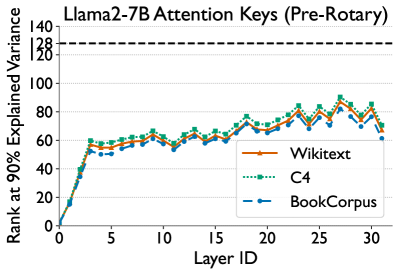
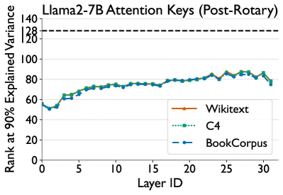
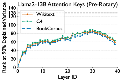
An intriguing trend is the variation in $Rank_{l}@90$ across layers for different models, indicating that the intrinsic dimensionality of the keys is not uniform across model layers. A potential future direction could be to investigate the reasons for this variation from a semantic perspective.

For a more fine-grained analysis, we plot the normalized eigenvalues of the covariance matrix of the keys for a few layers and heads of Llama2-7B, Mistral-7B, and Pythia-6.9B on the WikiText-2 dataset as an example in Figure 9. Here again, we observe that the explained variance significantly decreases after the initial principal dimensions. The results for the other models are similar to the ones shown here.

Figure 9: Normalized eigenvalues of the covariance matrix of the keys produced by Layer 1, Head 1 (top row), and Layer 28, Head 6 (bottom row) of Llama2-7B (left), Mistral-7B (middle), and Pythia-6.9B (right) on the WikiText-2 dataset. We observe that the explained variance significantly decreases after the initial principal dimensions. The dashed lines represent the rank at which 90% of the variance is explained ($Rank_{i,h}@90$).

A.2 Variation of Rank across Attention Heads

In this section, we discuss the variation of the rank at which 90% of the variance is explained ($Rank_{l}@90$) across different heads within a layer for two models: Llama2-7B and Mistral-7B. Figure 10 shows the heatmap of the $Rank_{l}@90$ for the pre-rotary (top) and post-rotary (bottom) keys across all layers and heads for Mistral-7B. We observe that the $Rank_{l}@90$ is considerably lower for pre-rotary keys vs post-rotary keys. Focusing on the pre-rotary keys, we see that the initial layers have a lower rank compared to the later layers. In each layer, there are some heads heads with high-rank values even though the median rank is low. This might indicate that some head in that layer is more important and uses more complex information about the keys. Interestingly for post-rotary keys, we see a pattern where 4 out of the 8 heads in each layer have the same rank. This might have to do with how the rotary embeddings are applied to Mistral-7B as we do not see this pattern in Llama2-7B.

Figure 11 shows the heatmap of the $Rank_{l}@90$ for the pre-rotary (left) and post-rotary (right) keys across all layers and heads for Llama2-7B. We observe a similar trend as Mistral-7B where the initial layers have a lower rank compared to the later layers. However, we do not see the same pattern in the post-rotary keys as we saw in Mistral-7B. This might indicate that the rotary embeddings are applied differently in Llama2-7B compared to Mistral-7B.

In this section, we examine the variation in the rank at which 90% of the variance is explained ($Rank_{l}@90$) across different heads within a layer for two models: Llama2-7B and Mistral-7B. Figure 10 shows the heatmap of $Rank_{l}@90$ for the pre-rotary (top) and post-rotary (bottom) keys across all layers and heads for Mistral-7B. We observe that the $Rank_{l}@90$ is significantly lower for pre-rotary keys compared to post-rotary keys. Focusing on the pre-rotary keys, it is evident that the initial layers exhibit lower rank values than the later layers. In each layer, some heads demonstrate high-rank values, even though the median rank remains low. This suggests that certain heads in those layers are more important and leverage more complex information about the keys. Interestingly, for the post-rotary keys, we notice a pattern in which 4 out of the 8 heads in each layer share the same rank. This phenomenon may be related to how rotary embeddings are applied in Mistral-7B, as we do not observe this pattern in Llama2-7B. Further investigation is needed to understand this trend.

Figure 11 illustrates the heatmap of $Rank_{l}@90$ for the pre-rotary (left) and post-rotary (right) keys across all layers and heads for Llama2-7B. A similar trend emerges as seen in Mistral-7B, where the initial layers have lower rank values compared to the later layers. However, the same pattern in post-rotary keys that was observed in Mistral-7B is absent here, suggesting that rotary embeddings may be applied differently in Llama2-7B compared to Mistral-7B.

For both the models, we can see that in each layer, there are some heads with very high-rank values, even when the median rank is low. This might indicate that some heads in that layer are more important and use more complex information about the keys. Analysis into chosing the best reduced dimensionality based upon the the distribution of ranks across heads could be a potential future direction.

Figure 10: Heatmap showing the rank at 90% explained variance for the pre-rotary(top) and post-rotary(bottom) key vectors across all layers and heads for Mistral-7B.

Figure 11: Heatmap showing the rank at 90% explained variance for the pre-rotary(top) and post-rotary(bottom) key vectors across all layers and heads for Llama2-7B.

A.3 Dimensionality Analysis for Queries and Values

Figure 12: Rank at which 90% of variance is explained ($Rank_{l}@90$) for the query vectors across various models and datasets.

Figure 13: Rank at which 90% of variance is explained ($Rank_{l}@90$) for the value vectors across various models and datasets.

While our main focus has been on the dimensionality of the keys, we also performed exploratory analysis on the dimensionality of the queries and values. Figures 12 and 13 show the $Rank_{l}@90$ for the queries and values, respectively, for Llama2-7B and Llama3-70B. We observe that the queries and values also exhibit low dimensionality across all layers and heads, similar to the keys, while values tend to have a considerably higher dimensionality and close to the full dimensionality of the value vectors. This observation can intuitively be explained by the fact that both keys and queries are used to compute the scalar attention scores and thus do not need to be high-dimensional, while values are weighted by these scores and used to compute the final output, and thus need to be high-dimensional to capture the complexity of the data.

Appendix B Comprehensive Evaluation Results

B.1 Performance of Loki on Perplexity and Short-Context Downstream Tasks

Figure 14: Performance of Loki on Perplexity (top) and Short-Context Downstream Task evaluation for different models using pre-rotary and post-rotary PCA transformation. For each model and each transform type, we run Loki with different values of $k$ and $d$.

Table 3: Performance of different models compared to hugging face baseline with different configurations of $k$ and $d$ using pre-rotary PCA transformation.

Model	Method	$k$	$d$	PPL$\downarrow$	Hellaswag$\uparrow$	TQA$\uparrow$	Winogrande$\uparrow$	ARC$\uparrow$	GSM8K$\uparrow$	MMLU$\uparrow$	Avg$\uparrow$
Llama2-7B	Full Attention	-	-	5.1101	75.99	38.96	69.06	46.33	13.87	41.84	47.67
Llama2-7B	Loki	0.5	0.5	5.1195	75.96	38.85	69.22	46.16	13.19	41.34	47.45
	Loki	0.5	0.25	5.1223	75.84	39.05	68.82	45.82	12.36	40.95	47.14
	Loki	0.5	0.125	5.1250	75.09	38.51	69.53	44.28	10.77	39.07	46.21
	Loki	0.25	0.5	5.1881	75.73	38.04	67.25	44.20	11.30	39.74	46.04
	Loki	0.25	0.25	5.2185	73.43	38.35	63.61	41.21	7.96	36.43	43.50
	Loki	0.25	0.125	5.3044	53.23	40.08	59.35	36.09	2.81	30.99	37.09
	Loki	0.125	0.5	5.4980	70.42	39.40	52.49	35.92	7.13	33.22	39.76
	Loki	0.125	0.25	6.0729	56.04	42.76	49.57	31.91	2.27	27.15	34.95
	Loki	0.125	0.125	8.0514	31.06	44.46	49.01	25.34	0.38	23.64	28.98
Llama2-13B	Full Attention	-	-	4.5680	79.38	36.90	72.22	49.15	22.97	52.06	52.11
Llama2-13B	Loki	0.5	0.5	4.5701	79.34	37.06	73.09	48.81	23.20	52.19	52.28
	Loki	0.5	0.25	4.5708	79.27	37.14	72.14	49.40	22.44	52.03	52.07
	Loki	0.5	0.125	4.5737	78.45	37.39	70.09	47.95	19.86	50.98	50.79
	Loki	0.25	0.5	4.5979	79.19	37.35	71.90	47.87	22.14	52.02	51.74
	Loki	0.25	0.25	4.6110	77.39	36.89	68.90	46.16	19.86	48.80	49.67
	Loki	0.25	0.125	4.6829	71.17	37.21	58.17	36.26	7.88	41.30	42.00
	Loki	0.125	0.5	4.8153	77.38	38.45	56.27	41.64	14.94	48.63	46.22
	Loki	0.125	0.25	5.3912	61.85	36.79	52.09	32.08	2.96	36.40	37.03
	Loki	0.125	0.125	7.6573	38.67	43.00	50.20	24.32	0.68	23.63	30.08
Llama2-70B	Full Attention	-	-	3.1205	83.82	44.81	77.90	57.34	53.15	65.41	63.74
Llama2-70B	Loki	0.5	0.5	3.1319	-	-	-	-	-	-	-
	Loki	0.5	0.25	3.1293	83.65	39.78	76.95	56.91	41.93	63.32	60.42
	Loki	0.5	0.125	3.1316	82.38	39.33	72.85	54.61	37.45	60.85	57.91
	Loki	0.25	0.5	3.2986	80.54	42.46	75.85	57.08	22.21	57.14	55.88
	Loki	0.25	0.25	3.2830	76.05	44.88	63.54	50.26	15.92	51.79	50.41
	Loki	0.25	0.125	3.4571	52.25	44.73	50.36	25.09	2.35	29.37	34.02
	Loki	0.125	0.5	3.8327	68.06	39.43	58.80	46.93	10.31	44.82	44.72
	Loki	0.125	0.25	3.9259	46.59	45.88	46.96	28.67	2.35	28.90	33.22
	Loki	0.125	0.125	6.4963	30.07	49.19	51.30	22.78	1.14	24.75	29.87
Llama3-8B	Full Attention	-	-	5.5696	79.17	43.89	72.93	53.24	50.11	62.19	60.26
Llama3-8B	Loki	0.5	0.5	5.5703	78.84	44.21	73.64	54.01	48.90	61.47	60.18
	Loki	0.5	0.25	5.5746	77.44	43.68	68.27	49.15	47.16	60.58	57.71
	Loki	0.5	0.125	5.5876	74.83	44.23	65.43	43.94	40.41	56.97	54.30
	Loki	0.25	0.5	5.5944	76.54	44.32	60.93	43.43	44.66	58.33	54.70
	Loki	0.25	0.25	5.6648	69.42	41.50	50.36	34.64	33.06	44.50	45.58
	Loki	0.25	0.125	6.0558	56.11	42.14	50.36	27.13	9.17	30.46	35.90
	Loki	0.125	0.5	5.7356	66.13	44.00	50.04	28.33	31.77	40.61	43.48
	Loki	0.125	0.25	6.5780	45.14	41.00	49.33	23.89	3.18	26.05	31.43
	Loki	0.125	0.125	11.1097	32.70	44.31	47.04	23.29	0.68	23.80	28.64
Llama3-70B	Full Attention	-	-	2.5653	84.89	45.57	80.43	64.33	80.67	75.03	71.82
Llama3-70B	Loki	0.5	0.5	2.5656	85.17	45.66	79.95	63.99	79.91	74.90	71.60
	Loki	0.5	0.25	2.5665	84.22	45.78	75.06	59.81	78.77	73.68	69.55
	Loki	0.5	0.125	2.5712	82.21	45.53	69.61	54.78	74.98	70.28	66.23
	Loki	0.25	0.5	2.5727	84.09	45.64	71.35	57.51	79.76	73.12	68.58
	Loki	0.25	0.25	2.5942	79.06	45.09	59.27	43.26	72.78	62.47	60.32
	Loki	0.25	0.125	2.7577	67.59	45.46	50.67	31.48	45.56	42.21	47.16
	Loki	0.125	0.5	2.6285	78.96	46.48	51.14	40.70	74.53	62.19	59.00
	Loki	0.125	0.25	2.8796	63.93	41.69	46.33	27.65	50.19	36.08	44.31
	Loki	0.125	0.125	4.1495	39.07	41.09	49.88	23.38	3.03	25.73	30.36
TinyLlama-1.1B	Full Attention	-	-	7.9671	60.45	37.88	60.22	32.85	1.90	24.86	36.36
TinyLlama-1.1B	Loki	0.5	0.5	8.0040	60.39	38.19	59.98	32.08	1.90	24.62	36.19
	Loki	0.5	0.25	8.0342	59.96	38.80	59.27	32.85	2.20	24.33	36.23
	Loki	0.5	0.125	8.1057	57.93	39.10	57.14	31.91	1.52	24.98	35.43
	Loki	0.25	0.5	8.3475	58.06	40.05	58.17	31.06	1.52	24.83	35.62
	Loki	0.25	0.25	8.6352	52.69	42.96	52.01	29.18	1.29	24.76	33.82
	Loki	0.25	0.125	9.4947	44.43	44.21	50.75	23.89	1.44	24.34	31.51
	Loki	0.125	0.5	9.3280	51.29	42.27	53.91	27.82	0.83	24.17	33.38
	Loki	0.125	0.25	11.5887	37.32	47.04	47.51	25.00	1.52	23.49	30.31
	Loki	0.125	0.125	19.9290	30.13	48.50	51.30	24.66	1.06	24.11	29.96
Mistral-7B	Full Attention	-	-	4.9140	81.07	42.62	73.95	53.92	38.59	59.65	58.30
Mistral-7B	Loki	0.5	0.5	4.9147	80.84	42.99	74.27	53.58	38.06	59.83	58.26
	Loki	0.5	0.25	4.9152	80.55	43.11	72.69	53.41	36.69	59.14	57.60
	Loki	0.5	0.125	4.9193	79.38	42.29	70.40	51.28	33.59	57.29	55.71
	Loki	0.25	0.5	4.9185	79.00	43.41	70.17	49.23	36.16	58.25	56.04
	Loki	0.25	0.25	4.9233	77.65	42.18	62.98	46.59	32.68	53.70	52.63
	Loki	0.25	0.125	4.9986	66.95	39.58	52.64	36.35	14.86	38.20	41.43
	Loki	0.125	0.5	4.9311	72.66	43.89	52.25	35.58	33.36	50.01	47.96
	Loki	0.125	0.25	4.9636	65.93	41.12	51.78	29.18	18.42	38.14	40.76
	Loki	0.125	0.125	5.7404	36.32	43.14	52.17	23.98	0.53	24.60	30.12
Mixtral-8x7B	Full Attention	-	-	3.5967	84.01	48.53	76.32	59.73	58.38	67.90	65.81
Mixtral-8x7B	Loki	0.5	0.5	3.5979	83.86	46.86	75.53	60.15	57.32	67.83	65.26
	Loki	0.5	0.25	3.6047	83.70	46.70	76.24	59.73	57.01	67.21	65.10
	Loki	0.5	0.125	3.6201	82.91	42.27	73.48	57.42	43.44	65.71	60.87
	Loki	0.25	0.5	3.6076	82.58	48.16	71.43	58.28	56.18	66.72	63.89
	Loki	0.25	0.25	3.6584	81.32	43.49	62.83	51.79	42.76	60.82	57.17
	Loki	0.25	0.125	3.9252	73.16	39.49	56.04	44.80	4.85	45.55	43.98
	Loki	0.125	0.5	3.6417	76.93	48.21	50.91	41.72	50.87	58.30	54.49
	Loki	0.125	0.25	3.8467	70.07	37.88	49.17	32.68	11.52	39.23	40.09
	Loki	0.125	0.125	6.9799	42.34	43.80	54.38	24.66	0.45	24.99	31.77

Table 4: Performance of different models compared to hugging face baseline with different configurations of $k$ and $d$ using post-rotary PCA transformation.

Model	Method	$k$	$d$	PPL$\downarrow$	Hellaswag$\uparrow$	TQA$\uparrow$	Winogrande$\uparrow$	ARC$\uparrow$	GSM8K$\uparrow$	MMLU$\uparrow$	Avg$\uparrow$
Llama2-7B	Full Attention	-	-	5.1101	75.99	38.96	69.06	46.33	13.87	41.84	47.67
Llama2-7B	Loki	0.5	0.5	5.1195	75.91	38.87	68.59	46.50	14.10	41.49	47.58
	Loki	0.5	0.25	5.1206	75.84	39.05	68.82	45.82	12.36	40.95	47.14
	Loki	0.5	0.125	5.1241	75.48	38.77	67.64	43.94	12.59	38.85	46.21
	Loki	0.25	0.5	5.1838	75.19	38.16	62.12	41.21	10.69	40.42	44.63
	Loki	0.25	0.25	5.2017	72.59	39.16	56.59	37.37	10.24	37.74	42.28
	Loki	0.25	0.125	5.4428	68.49	38.83	56.51	32.17	10.92	32.68	39.93
	Loki	0.125	0.5	5.3601	70.42	39.40	52.49	35.92	7.13	33.22	39.76
	Loki	0.125	0.25	5.5606	59.98	41.72	48.86	26.96	6.22	28.38	35.35
	Loki	0.125	0.125	7.4062	40.14	43.84	49.64	25.43	5.99	24.13	31.53
Llama2-13B	Full Attention	-	-	4.5680	79.38	36.90	72.22	49.15	22.97	52.06	52.78
Llama2-13B	Loki	0.5	0.5	4.5731	79.34	37.06	73.09	48.81	23.20	52.19	52.28
	Loki	0.5	0.25	4.5737	79.05	37.46	72.69	48.29	23.58	51.94	52.17
	Loki	0.5	0.125	4.5745	78.45	37.39	70.09	47.95	19.86	50.98	50.79
	Loki	0.25	0.5	4.5937	79.19	37.35	71.90	47.87	22.14	52.02	51.74
	Loki	0.25	0.25	4.6102	77.39	36.89	68.90	46.16	19.86	48.80	49.67
	Loki	0.25	0.125	4.8082	61.52	38.10	52.41	26.54	20.85	44.69	40.68
	Loki	0.125	0.5	4.7029	77.38	38.45	56.27	41.64	14.94	48.63	46.22
	Loki	0.125	0.25	4.9668	72.71	40.09	51.14	33.28	9.10	39.20	40.92
	Loki	0.125	0.125	6.1436	34.81	46.07	52.09	24.15	8.79	26.50	32.07
Llama2-70B	Full Attention	-	-	3.1205	83.82	44.81	77.90	57.34	53.15	65.41	63.74
Llama2-70B	Loki	0.5	0.5	3.1411	83.89	41.32	78.06	57.68	50.42	64.75	62.69
	Loki	0.5	0.25	3.1453	83.69	43.42	76.80	56.31	52.99	64.73	62.99
	Loki	0.5	0.125	3.1457	83.41	43.51	75.45	55.89	52.54	64.12	62.49
	Loki	0.25	0.5	3.4619	82.36	41.91	76.87	56.48	42.61	60.11	60.06
	Loki	0.25	0.25	3.5701	81.42	45.26	71.11	49.74	44.28	59.56	58.56
	Loki	0.25	0.125	3.5459	80.59	45.57	65.59	49.15	46.93	58.00	57.64
	Loki	0.125	0.5	4.1427	71.90	44.59	58.09	41.98	34.34	50.30	50.20
	Loki	0.125	0.25	4.7796	67.03	46.58	51.85	32.17	37.30	42.21	46.19
	Loki	0.125	0.125	4.6898	64.84	44.89	50.51	29.95	38.74	39.08	44.67
Llama3-8B	Full Attention	-	-	5.5696	79.17	43.89	72.93	53.24	50.11	62.19	60.26
Llama3-8B	Loki	0.5	0.5	5.5699	76.03	43.83	67.32	44.71	49.36	59.38	56.77
	Loki	0.5	0.25	5.9343	72.55	42.67	61.64	39.93	41.09	57.88	52.63
	Loki	0.5	0.125	5.7429	71.38	43.16	58.64	40.61	39.42	57.14	51.72
	Loki	0.25	0.5	5.6783	68.02	42.07	48.78	31.31	43.59	48.06	46.97
	Loki	0.25	0.25	11.4459	57.39	42.13	48.70	27.90	28.28	38.69	40.52
	Loki	0.25	0.125	13.2883	48.99	42.10	48.07	22.87	12.81	30.90	34.29
	Loki	0.125	0.5	6.8023	49.68	41.14	49.25	25.51	31.39	30.86	37.97
	Loki	0.125	0.25	16.3507	36.39	43.62	50.04	25.09	16.60	26.21	32.99
	Loki	0.125	0.125	22.6596	31.60	46.38	49.25	23.12	1.14	23.61	29.18
Llama3-70B	Full Attention	-	-	2.5653	84.89	45.57	80.43	64.33	80.67	75.03	71.82
Llama3-70B	Loki	0.5	0.5	2.5660	83.60	45.83	72.61	56.14	79.15	73.43	68.46
	Loki	0.5	0.25	2.5697	79.92	46.22	62.90	48.46	78.39	71.11	64.50
	Loki	0.5	0.125	2.7810	76.66	46.77	59.27	42.66	56.94	68.48	58.46
	Loki	0.25	0.5	2.5742	74.91	47.67	51.54	38.05	77.71	64.14	59.00
	Loki	0.25	0.25	2.8593	61.40	47.86	48.38	27.73	67.32	41.18	48.98
	Loki	0.25	0.125	5.6725	41.90	47.18	47.59	23.29	5.31	26.98	32.04
	Loki	0.125	0.5	2.6231	56.24	43.91	50.51	24.66	72.48	38.52	47.72
	Loki	0.125	0.25	4.2512	31.91	47.39	50.43	24.57	19.71	24.72	33.12
	Loki	0.125	0.125	57.6788	27.01	49.28	50.67	24.06	0.68	24.76	29.41
TinyLlama-1.1B	Full Attention	-	-	7.9671	60.45	37.88	60.22	32.85	1.90	24.86	36.36
TinyLlama-1.1B	Loki	0.5	0.5	7.9979	60.17	38.14	58.33	31.57	1.90	25.12	35.87
	Loki	0.5	0.25	8.0135	58.78	39.95	54.38	30.55	1.29	24.58	34.92
	Loki	0.5	0.125	8.0414	57.77	38.20	54.93	30.89	1.44	24.39	34.60
	Loki	0.25	0.5	8.3190	57.35	37.87	53.83	29.69	1.67	25.13	34.26
	Loki	0.25	0.25	8.5687	52.40	40.86	49.33	26.96	2.20	23.34	32.51
	Loki	0.25	0.125	8.8956	51.19	42.07	52.96	28.92	0.91	25.10	33.52
	Loki	0.125	0.5	8.9679	51.32	38.24	50.20	24.23	1.29	24.92	31.70
	Loki	0.125	0.25	10.2592	42.85	39.06	51.85	25.60	1.52	24.06	30.82
	Loki	0.125	0.125	11.3508	39.27	41.55	50.67	22.78	0.45	24.50	29.87
Mistral-7B	Full Attention	-	-	4.9140	81.07	42.62	73.95	53.92	38.59	59.65	58.30
Mistral-7B	Loki	0.5	0.5	4.9149	79.89	42.15	70.56	49.83	37.45	58.00	56.31
	Loki	0.5	0.25	4.9221	78.99	40.84	63.06	45.48	33.43	55.15	52.82
	Loki	0.5	0.125	4.9317	73.88	40.58	57.06	33.87	22.06	45.95	45.57
	Loki	0.25	0.5	5.2052	71.86	40.74	56.04	38.91	24.18	45.56	46.22
	Loki	0.25	0.25	6.5445	62.62	38.93	48.62	25.17	1.82	30.80	34.66
	Loki	0.25	0.125	7.7609	35.51	43.67	53.20	23.63	1.06	23.86	30.16
	Loki	0.125	0.5	9.5167	51.73	45.44	51.62	25.77	3.03	27.99	34.26
	Loki	0.125	0.25	13.5597	34.85	46.38	50.20	22.53	0.45	23.60	29.67
	Loki	0.125	0.125	20.5289	28.52	51.98	50.91	26.96	0.45	23.64	30.41
Mixtral-8x7B	Full Attention	-	-	3.5967	84.01	48.53	76.32	59.73	58.38	67.90	65.81
Mixtral-8x7B	Loki	0.5	0.5	3.5970	83.24	47.32	74.27	58.53	56.48	67.23	64.51
	Loki	0.5	0.25	3.6196	81.71	43.51	69.61	53.67	55.57	63.92	61.33
	Loki	0.5	0.125	3.6635	76.18	41.63	61.72	47.78	49.28	58.94	55.92
	Loki	0.25	0.5	3.6004	79.99	46.47	61.64	49.15	57.85	63.04	59.69
	Loki	0.25	0.25	3.7906	71.58	37.77	53.28	37.54	37.38	46.66	47.37
	Loki	0.25	0.125	4.2566	59.23	36.58	50.75	28.67	15.39	32.28	37.15
	Loki	0.125	0.5	3.6358	72.29	45.28	50.67	33.70	55.50	47.15	50.76
	Loki	0.125	0.25	4.5500	52.16	37.86	46.57	23.98	17.13	27.02	34.12
	Loki	0.125	0.125	5.5250	46.93	40.33	49.72	23.55	0.91	24.78	31.04

In this section, we provide a detailed evaluation of our method across a wide range of models and tasks. Figure 14 illustrates the performance of Loki on perplexity and downstream tasks compared to the full attention baseline. We present results for both pre-rotary and post-rotary PCA transformations. The models evaluated include Llama2-7B, Llama2-13B, Llama2-70B, Llama3-8B, Llama3-70B, TinyLlama-1.1B, Mistral-7B, and Mixtral-8x7B. We assess the models using various configurations of $k$ and $d$ for Loki.

As $k_{f}$ and $d_{f}$ decrease, the model’s performance deteriorates, particularly when both are set to 0.125. Notably, the impact of $k_{f}$ on performance is more pronounced than that of $d_{f}$. This is evident as $k_{f}=0.125$ and $d_{f}=0.5$ significantly underperform compared to $k_{f}=0.5$ and $d_{f}=0.125$ across nearly all models. The configurations of $k_{f}=0.25$ and $d_{f}=0.25$, along with $k_{f}=0.125$ and $d_{f}=0.5$, demonstrate relatively strong performance across all models, striking a favorable balance between performance and accuracy, with a theoretical speedup of 2.6x for both configurations. Settings with $k_{f}=0.5$ maintain model quality much more effectively but do not yield a significant empirical speedup.

Tables 3 and 4 present finer-grained results for each task and model.

B.2 Variable Dimensionality Analysis

Figure 15: Average short-context task accuracies using fixed $d_{f}$ vs. varying $d_{f}$ values across the layers for Llama2-7B (left), Llama2-13B (middle) and Llama3-8B (right). For the variable policy, $d_{f}$ is set based on per-layer explained variance (varied from 0.5 to 0.8). Compression ratio is the average $d_{f}/D$ across layers.

In this section, we present our experiments utilizing a variable $d_{f}$ policy per layer in Loki. For this experiment, we set $d_{f}$ based on the per-layer explained variance, varying from 0.5 to 0.8, and plotted the average short-context task accuracies (refer to Section 5) against the compression ratio, calculated as follows:

$$\text{Compression Ratio}=\frac{\sum_{l=1}^{L}d_{f}^{l}}{D}$$ (6)

Figure 15 presents these plots for the Llama2-7B, Llama2-13B, and Llama3-8B models. We observe that the variable $d_{f}$ policy does not yield significant improvements over the fixed $d_{f}$ policy used in our experiments. It is possible that different layers may require distinct explained variance thresholds for optimal performance, indicating that further tuning is necessary. Nevertheless, the simplicity of the fixed $d_{f}$ policy, combined with its comparable performance to the variable $d_{f}$ policy, makes it a practical choice for Loki.

Appendix C Comparison of our kernels with SparQ

As mentioned in Section 4.3, we create optimized kernels in Triton to efficiently compute the three matrix multiplications in Loki (lines 5, 8, and 9 of Algorithm 1) without creating temporary dense copies of subsets of the KV-cache. Initially, we planned to use the implementations developed by the authors of SparQ [26]. However, we discovered two major issues with their kernels. Let’s say you are multiplying two matrices of sizes $m\times k$ and $k\times n$, then SparQ kernels parallelize compute along only the m dimension. However, it is well known that one can parallelize matrix multiplications along the n dimension as well and gain more performance. Thus, we add this extra dimension of parallelism to their triton kernel. Second, their kernels cannot handle non-powers of 2 number of tokens in the KV-cache, a setting which is commonly encountered in inference since we generated keys and values one at a time. Therefore, we extend their kernels to handle non-powers of two number of tokens in the KV-cache successfully. In Figure 16, we compare the performance of our kernel with SparQand vanilla PyTorch based attention for an attention layer in Llama2-7B for various sizes of the KV-cache ranging from 512 to 4096. We do this for the matmul operation of query and keys with top-$k$ as 0.25.

Figure 16: Comparing the performance of our proposed kernel for computing $Q.K^{T}$, with SparQ’s [26] kernel for various batch sizes and number of keys in the KV-cache.

We see very high speedups over SparQ for small batch sizes. For instance, for a batch size of 1 with 4096 keys (bottom right), our kernel is faster than SparQ by nearly $2.8\times$! Infact, the SparQ kernel barely obtains any speedup over vanilla PyTorch even though it is only using 25% of the keys (1024 out of 4096). This is because SparQ only parallelizes compute across the m-dimension as we discussed before. In attention the m-dimension is proportional to the batch size, and thus having a small batch size limits the amount of parallelism SparQ kernels can exploit. Whereas, given our 2D parallel approach to matrix multiplication, we can exploit parallelism along the sequence dimension and thus still obtain significant speedups over vanilla PyTorch. Note that smaller batch sizes are very common in inference and hence it is extremely important to design a kernel that can function efficiently even at smaller batch sizes. Our speedups over SparQ decrease with larger batch sizes, but overall we are always faster than both SparQ and vanilla PyTorch.

Appendix D Generation Examples

In this section, we look at a generation example from the Llama2-7B (Chat) model given a custom prompt for different settings of $k$ and $d$.

Appendix E PCAAttn: Directly Leveraging Reduced-Dimensional Attention Scores

Algorithm 2 PCAAttn

1: At the $i^{th}$ step - Input: $\mathbf{x}_{S}\in\mathbb{R}^{1\times D}$, KV-cache: $\mathbf{\hat{K}}_{:S-1,:d},\mathbf{V}_{:S-1}\in\mathbb{R}^{(S-1)\times d}$, Projection Matrix: $\mathbf{P}_{:d}\in\mathbb{R}^{D\times d}$ (first $d$ principal components)

2: function PCA-Attention($\mathbf{x}_{S},\mathbf{\hat{K}}_{:S-1,:d},\mathbf{V}_{i-1},\mathbf{P}_{d}$)

3:   $\mathbf{q}_{S},\mathbf{k}_{S},\mathbf{v}_{S}\leftarrow computeQKV(\mathbf{x}_{S})$

4:   $\mathbf{\hat{q}}_{S,:d}\leftarrow\mathbf{q}_{S}\mathbf{P}_{:d}$, $\mathbf{\hat{k}}_{S,:d}\leftarrow\mathbf{k}_{S}\mathbf{P}_{:d}$

5:   $\mathbf{\hat{K}}_{:S,:d}\leftarrow concat(\mathbf{\hat{K}}_{:S-1,:d},\mathbf{\hat{k}}_{S,:d})$

6:   $\mathbf{V}_{:S}\leftarrow concat(\mathbf{V}_{:S-1},\mathbf{v}_{S})$

7:   $\mathbf{a}=softmax(\frac{\mathbf{\hat{q}}_{S,:d}(\mathbf{\hat{K}}_{:S,:d})^{T}}{\sqrt{D}})$

8:   return $\mathbf{a}\mathbf{V}_{:S}$

9: end function

One other approach we tried is to directly use the formulation in 4.1 to compute the final attention scores. More specifically, we compute the PCA transformed query and key vectors, projected onto the first $d$ principal components, and then compute the attention scores. We only store the reduced dimension key vectors in the KV-cache. We call this method PCAAttn (Algorithm 2).

Compute and Memory Analysis: When computing attention between a single query $\mathbf{q}_{S}\in\mathbb{R}^{1\times D}$ and the key vectors $\mathbf{K}_{:S}\in\mathbb{R}^{S\times D}$, the matrix multiplication $\mathbf{q}_{S}\mathbf{K}_{:S}^{T}$ has a complexity of $\mathcal{O}(DS)$. Using PCAAttn, the key and query vectors are reduced to $d$ dimensions and the complexity of the matrix multiplication is reduced to $\mathcal{O}(dS)$. Thus, we can get a speedup of $D/d$ in the attention dot product computation. The PCA transformation of the query and key vector generated at each step has a complexity of $\mathcal{O}(D^{2})$, which is small when $S>>D$. The KV-cache memory requirement is reduced by a factor of $0.5*D/d$ because we only reduce the key vectors to $d$ dimensions and not the values. Additionally, the PCA adds a significantly small memory overhead of $\mathcal{O}(Dd)$.

Experimental Results:

Table 5: Performance of PCAAttn with various cache configurations.

Model	Method	$k_{f}$	$d_{f}$	Perplexity$\downarrow$	Hellaswag$\uparrow$	Winogrande $\uparrow$	MathQA $\uparrow$	OpenbookQA $\uparrow$	RTE $\uparrow$	COPA $\uparrow$
Llama2-7B	Full Attention	-	-	5.1102	57.2	69.1	28.4	31.4	62.8	87.0
Llama2-7B	Exact TopK	0.5	-	5.1191	57.2	68.9	28.3	31.2	63.9	86.0
	H2O	0.5	-	5.1456	55.5	61.8	24.4	27.4	62.8	77.0
	PCAAttn	-	0.5	38.3997	33.3	53.2	21.7	14.2	50.5	73
Llama2-7B	Exact TopK	0.25	-	5.1799	56.9	68.6	29.4	29	66.4	76.0
	H2O	0.25	-	5.2809	50.1	51.6	21.1	17.8	55.2	55.0
	PCAAttn	-	0.25	243.2631	26.9	48.5	20.5	11.4	49.1	65.0
Mistral-7B	Full Attention	-	-	4.9140	61.2	73.9	35.7	32.2	66.8	91.0
Mistral-7B	Exact TopK	0.5	-	4.9143	61.1	73.8	35.6	32.6	65.3	92.0
	H2O	0.5	-	4.9560	59.4	58.6	26.4	23.0	62.4	71.0
	PCAAttn	-	0.5	396.8967	31.4	50.4	22.5	15.6	53.4	72.0
Mistral-7B	Exact TopK	0.25	-	4.9170	60.4	73.0	35.4	30.0	65.3	85.0
	H2O	0.25	-	5.0805	52.7	49.7	21.9	17.4	52.0	56.0
	PCAAttn	-	0.25	933.6016	27.2	52.2	21.6	13.6	53.0	63.0

Table 5 shows the performance of PCAAttn on Llama2-7B and Mistral-7B models. We can see that our PCAAttn method performs poorly compared to all the baselines and the H₂O method for all cache configurations. We believe that this happens because the application of rotary embeddings increases the dimensionality of the key vectors and using reduced dimensionality to store the keys results in loss of information. To further investigate this, we look back at Figure 10 which shows the rank at 90% explained variance for the key vectors across all layers and heads. Even though, the average rank per layer is around 50% of the full dimensionality, the rank for some layers and especially some heads within each layer is much higher. Due to the poor performance of PCAAttn, we do not include it in the final results and decide to focus on Loki instead in the main paper. Note, that we only tried the post-rotary transformations in PCAAttn, and it is possible that pre-rotary transformations might perform better, but we leave this for future work.

Appendix F Estimate of Compute Resources Required to Replicate our Experiments

As mentioned in Section 6, we conduct all of our experiments on Perlmutter, a multi-GPU cluster with 4 A100 GPUs per node. Since we do not do any training/fine-tuning, our experiments can be done on a very small number of GPUs. For instance, all of our runs involving models with 7B and 13B parameters were done on a single A100 GPU. For models larger than this (like LLama2-70B, Llama3-70B), we had to resort to running on four A100 GPUs (or a single node) with tensor parallelism using the AxoNN parallel deep learning framework. All results for 7B and 13B sized models can be compiled within 3 hours. For larger models like the 70B Llama-2 and 3 as well as Mixtral models, the total times for computing all results are in the ballpark of 10 hours. Our compute benchmarking runs of Llama-13B are very short and can be completed within 5 minutes.

References

- [1] Introducing triton: Open-source gpu programming for neural networks. https://openai.com/index/triton/, 2021.
- [2] Yushi Bai, Xin Lv, Jiajie Zhang, Hongchang Lyu, Jiankai Tang, Zhidian Huang, Zhengxiao Du, Xiao Liu, Aohan Zeng, Lei Hou, Yuxiao Dong, Jie Tang, and Juanzi Li. Longbench: A bilingual, multitask benchmark for long context understanding. arXiv preprint arXiv:2308.14508, 2023.
- [3] Edward Beeching, Clémentine Fourrier, Nathan Habib, Sheon Han, Nathan Lambert, Nazneen Rajani, Omar Sanseviero, Lewis Tunstall, and Thomas Wolf. Open llm leaderboard. https://huggingface.co/spaces/open-llm-leaderboard-old/open_llm_leaderboard, 2023.
- [4] Stella Biderman, Hailey Schoelkopf, Quentin Gregory Anthony, Herbie Bradley, Kyle O’Brien, Eric Hallahan, Mohammad Aflah Khan, Shivanshu Purohit, USVSN Sai Prashanth, Edward Raff, et al. Pythia: A suite for analyzing large language models across training and scaling. In International Conference on Machine Learning, pages 2397–2430. PMLR, 2023.
- [5] Rewon Child, Scott Gray, Alec Radford, and Ilya Sutskever. Generating long sequences with sparse transformers. arXiv preprint arXiv:1904.10509, 2019.
- [6] Krzysztof Choromanski, Valerii Likhosherstov, David Dohan, Xingyou Song, Andreea Gane, Tamas Sarlos, Peter Hawkins, Jared Davis, Afroz Mohiuddin, Lukasz Kaiser, David Belanger, Lucy Colwell, and Adrian Weller. Rethinking attention with performers, 2022.
- [7] Tri Dao, Dan Fu, Stefano Ermon, Atri Rudra, and Christopher Ré. Flashattention: Fast and memory-efficient exact attention with io-awareness. Advances in Neural Information Processing Systems, 35:16344–16359, 2022.
- [8] Abhimanyu Dubey, Abhinav Jauhri, Abhinav Pandey, Abhishek Kadian, Ahmad Al-Dahle, et al. The llama 3 herd of models, 2024.
- [9] Leo Gao, Jonathan Tow, Baber Abbasi, Stella Biderman, Sid Black, Anthony DiPofi, Charles Foster, Laurence Golding, Jeffrey Hsu, Alain Le Noac’h, Haonan Li, Kyle McDonell, Niklas Muennighoff, Chris Ociepa, Jason Phang, Laria Reynolds, Hailey Schoelkopf, Aviya Skowron, Lintang Sutawika, Eric Tang, Anish Thite, Ben Wang, Kevin Wang, and Andy Zou. A framework for few-shot language model evaluation, 12 2023.
- [10] Suyu Ge, Yunan Zhang, Liyuan Liu, Minjia Zhang, Jiawei Han, and Jianfeng Gao. Model tells you what to discard: Adaptive kv cache compression for llms. arXiv preprint arXiv:2310.01801, 2023.
- [11] Suyu Ge, Yunan Zhang, Liyuan Liu, Minjia Zhang, Jiawei Han, and Jianfeng Gao. Model tells you what to discard: Adaptive kv cache compression for llms, 2024.
- [12] Ankit Gupta, Guy Dar, Shaya Goodman, David Ciprut, and Jonathan Berant. Memory-efficient transformers via top-k attention. CoRR, abs/2106.06899, 2021.
- [13] Edward J. Hu, Yelong Shen, Phillip Wallis, Zeyuan Allen-Zhu, Yuanzhi Li, Shean Wang, and Weizhu Chen. Lora: Low-rank adaptation of large language models. CoRR, abs/2106.09685, 2021.
- [14] Benoit Jacob, Skirmantas Kligys, Bo Chen, Menglong Zhu, Matthew Tang, Andrew Howard, Hartwig Adam, and Dmitry Kalenichenko. Quantization and training of neural networks for efficient integer-arithmetic-only inference, 2017.
- [15] Albert Q Jiang, Alexandre Sablayrolles, Arthur Mensch, Chris Bamford, Devendra Singh Chaplot, Diego de las Casas, Florian Bressand, Gianna Lengyel, Guillaume Lample, Lucile Saulnier, et al. Mistral 7b. arXiv preprint arXiv:2310.06825, 2023.
- [16] Albert Q. Jiang, Alexandre Sablayrolles, Antoine Roux, Arthur Mensch, Blanche Savary, Chris Bamford, Devendra Singh Chaplot, Diego de las Casas, Emma Bou Hanna, Florian Bressand, Gianna Lengyel, Guillaume Bour, Guillaume Lample, Lélio Renard Lavaud, Lucile Saulnier, Marie-Anne Lachaux, Pierre Stock, Sandeep Subramanian, Sophia Yang, Szymon Antoniak, Teven Le Scao, Théophile Gervet, Thibaut Lavril, Thomas Wang, Timothée Lacroix, and William El Sayed. Mixtral of experts, 2024.
- [17] Nikita Kitaev, Łukasz Kaiser, and Anselm Levskaya. Reformer: The efficient transformer. arXiv preprint arXiv:2001.04451, 2020.
- [18] Woosuk Kwon, Zhuohan Li, Siyuan Zhuang, Ying Sheng, Lianmin Zheng, Cody Hao Yu, Joseph E. Gonzalez, Hao Zhang, and Ion Stoica. Efficient memory management for large language model serving with pagedattention. In Proceedings of the ACM SIGOPS 29th Symposium on Operating Systems Principles, 2023.
- [19] Wonbeom Lee, Jungi Lee, Junghwan Seo, and Jaewoong Sim. InfiniGen: Efficient generative inference of large language models with dynamic KV cache management. In 18th USENIX Symposium on Operating Systems Design and Implementation (OSDI 24), pages 155–172, Santa Clara, CA, July 2024. USENIX Association.
- [20] Zichang Liu, Aditya Desai, Fangshuo Liao, Weitao Wang, Victor Xie, Zhaozhuo Xu, Anastasios Kyrillidis, and Anshumali Shrivastava. Scissorhands: Exploiting the persistence of importance hypothesis for llm kv cache compression at test time. arXiv preprint arXiv:2305.17118, 2023.
- [21] Stephen Merity, Caiming Xiong, James Bradbury, and Richard Socher. Pointer sentinel mixture models. CoRR, abs/1609.07843, 2016.
- [22] Microsoft. Introducing phi-3: Redefining what’s possible with slms. https://azure.microsoft.com/en-us/blog/introducing-phi-3-redefining-whats-possible-with-slms/, 2024.
- [23] Markus Nagel, Marios Fournarakis, Rana Ali Amjad, Yelysei Bondarenko, Mart van Baalen, and Tijmen Blankevoort. A white paper on neural network quantization, 2021.
- [24] NERSC. Perlmutter system architecture. https://docs.nersc.gov/systems/perlmutter/architecture/.
- [25] Colin Raffel, Noam Shazeer, Adam Roberts, Katherine Lee, Sharan Narang, Michael Matena, Yanqi Zhou, Wei Li, and Peter J. Liu. Exploring the limits of transfer learning with a unified text-to-text transformer, 2023.
- [26] Luka Ribar, Ivan Chelombiev, Luke Hudlass-Galley, Charlie Blake, Carlo Luschi, and Douglas Orr. Sparq attention: Bandwidth-efficient llm inference, 2023.
- [27] Siddharth Singh and Abhinav Bhatele. AxoNN: An asynchronous, message-driven parallel framework for extreme-scale deep learning. In Proceedings of the IEEE International Parallel & Distributed Processing Symposium, IPDPS ’22. IEEE Computer Society, May 2022.
- [28] Siddharth Singh, Prajwal Singhania, Aditya K. Ranjan, Zack Sating, and Abhinav Bhatele. A 4d hybrid algorithm to scale parallel training to thousands of gpus, 2024.
- [29] Jianlin Su, Yu Lu, Shengfeng Pan, Ahmed Murtadha, Bo Wen, and Yunfeng Liu. Roformer: Enhanced transformer with rotary position embedding, 2023.
- [30] Mingjie Sun, Xinlei Chen, J. Zico Kolter, and Zhuang Liu. Massive activations in large language models, 2024.
- [31] Hugo Touvron et al. Llama 2: Open foundation and fine-tuned chat models. Technical report, 2023.
- [32] Ashish Vaswani, Noam Shazeer, Niki Parmar, Jakob Uszkoreit, Llion Jones, Aidan N. Gomez, Lukasz Kaiser, and Illia Polosukhin. Attention is all you need. CoRR, abs/1706.03762, 2017.
- [33] Sinong Wang, Belinda Z. Li, Madian Khabsa, Han Fang, and Hao Ma. Linformer: Self-attention with linear complexity, 2020.
- [34] Thomas Wolf, Lysandre Debut, Victor Sanh, Julien Chaumond, Clement Delangue, Anthony Moi, Pierric Cistac, Tim Rault, Rémi Louf, Morgan Funtowicz, Joe Davison, Sam Shleifer, Patrick von Platen, Clara Ma, Yacine Jernite, Julien Plu, Canwen Xu, Teven Le Scao, Sylvain Gugger, Mariama Drame, Quentin Lhoest, and Alexander M. Rush. Transformers: State-of-the-art natural language processing. In Proceedings of the 2020 Conference on Empirical Methods in Natural Language Processing: System Demonstrations, pages 38–45, Online, October 2020. Association for Computational Linguistics.
- [35] Guangxuan Xiao, Yuandong Tian, Beidi Chen, Song Han, and Mike Lewis. Efficient streaming language models with attention sinks. arXiv preprint arXiv:2309.17453, 2023.
- [36] Guangxuan Xiao, Yuandong Tian, Beidi Chen, Song Han, and Mike Lewis. Efficient streaming language models with attention sinks, 2024.
- [37] Zhewei Yao, Xiaoxia Wu, Cheng Li, Stephen Youn, and Yuxiong He. Zeroquant-v2: Exploring post-training quantization in llms from comprehensive study to low rank compensation. 2023.
- [38] Peiyuan Zhang, Guangtao Zeng, Tianduo Wang, and Wei Lu. Tinyllama: An open-source small language model. Technical report, 2024.
- [39] Zhenyu Zhang, Ying Sheng, Tianyi Zhou, Tianlong Chen, Lianmin Zheng, Ruisi Cai, Zhao Song, Yuandong Tian, Christopher Ré, Clark Barrett, et al. H o: Heavy-hitter oracle for efficient generative inference of large language models. arXiv preprint arXiv:2306.14048, 2023.
- [40] Yukun Zhu, Ryan Kiros, Richard Zemel, Ruslan Salakhutdinov, Raquel Urtasun, Antonio Torralba, and Sanja Fidler. Aligning books and movies: Towards story-like visual explanations by watching movies and reading books, 2015.