arXiv is now an independent nonprofit! Learn more
License: arXiv.org perpetual non-exclusive license
arXiv:2405.17392v4 [math.AP] 18 Aug 2025

Rigorous fast signal diffusion limit and convergence rates with the initial layer effect in a competitive chemotaxis system

Cordula Reisch Note: Email: c.reisch@tu-bs.de    Bao-Ngoc Tran Note: Email: bao-ngoc.tran@uni-graz.at (Corresponding author)    Juan Yang Note: Email: yangjuan12@sjtu.edu.cn
Abstract

We study a chemotaxis system that includes two competitive prey and one predator species in a two-dimensional domain, where the movement of prey (resp. predators) is driven by chemicals secreted by predators (resp. prey), called mutually repulsive (resp. mutually attractive) chemotactic effect. The kinetics for all species are chosen according to the competitive Lotka–Volterra equations for prey and to a Holling type functional response for the predator. Under the biologically relevant scenario that the chemicals diffuse much faster than the individual diffusion of all species and a suitable re-scaling, equations for chemical concentrations are parabolic with slow evolution depending on the relaxation time 0<ε≪10<\varepsilon\ll 1. The first main result shows the global existence of a unique classical solution to the system for each ε\varepsilon. Second, we study rigorously the so-called fast signal diffusion limit, passing from the system including parabolic equations with the slow evolution of the chemical concentrations to elliptic equations for the chemical concentrations, i.e. the limit as ε→0\varepsilon\to 0. This explains why elliptic equations can be proposed for chemical concentration instead of parabolic ones with slow evolution. Third, the L∞L^{\infty}-in-time convergence rates for the fast signal diffusion limit are estimated, where the effect of the initial layer is carefully treated. Finally, the differences between the systems with and without the slow evolution, and between the systems with one or two prey, as well as their dynamics, are discussed numerically.

Keywords: Competitive chemotaxis system, Fast signal diffusion limit, L∞L^{\infty}-in-time convergence rate, Singular limits, Bootstrap arguments.

2020 Mathematics Subject Classification: 35B25, 35A01, 35Q92, 92C17.

aInstitute for Partial Differential Equations, Technische Universität Braunschweig,
38106 Braunschweig, Germany

bDepartment of Mathematics and Scientific Computing, University of Graz,
Heinrichstrasse 36, 8010 Graz, Austria

cDepartment of Mathematics, Faculty of Science, Nong Lam University, Ho Chi Minh City, Vietnam

dSchool of Mathematical Sciences, Shanghai Jiao Tong University, Shanghai 200240, China

eSchool of Mathematics and Statistics, Lanzhou University, Lanzhou, 730000, China

1 Introduction

1.1 Food chain chemotaxis model

Chemotaxis is well-known and plays a crucial role in many biological systems in which the species’ movement is biased along concentration gradients of chemical stimuli. In the last decade, chemotaxis systems have gained much attention in mathematical analysis, such as, in two dimensions, global existence results for a parabolic-elliptic system can be found in [ZM17], or for a parabolic-parabolic system in [Bla17]. For a higher-dimensional case, the global existence was established in [GNU24, ZM17] by imposing restrictive conditions on parameters. Various results regarding global existence, large-time behaviour, or blowing-up of solutions have been studied in [TW15, PWZW20, TTQ21, YTY22, GNU24] and references therein. Recently, a chemotaxis system including two competitive prey and one predator species has been studied in [ABOV23] with a result on global existence and in [BOSV20] with numerical analysis, which will be studied in this paper in the context of fast signalling. Specifically, we consider in Q∞=Ω×(0,∞)Q_{\infty}=\Omega\times(0,\infty) the system

{∂τu~1−d~1Δu~1−χ~1∇⋅(u~1∇v~3)=f~1​(u~1,u~2,u~3),∂τu~2−d~2Δu~2−χ~2∇⋅(u~2∇v~3)=f~2​(u~1,u~2,u~3),∂τu~3−d~3Δu~3+∑i=12χ~3​i∇⋅(u~3∇v~i)=f~3​(u~1,u~2,u~3),\displaystyle\left\{\begin{array}[]{llll}\partial_{\tau}\widetilde{u}_{1}-\widetilde{d}_{1}\Delta\widetilde{u}_{1}-\widetilde{\chi}_{1}\nabla\cdot(\widetilde{u}_{1}\nabla\widetilde{v}_{3})&\hskip-5.69046pt=&\widetilde{f}_{1}(\widetilde{u}_{1},\widetilde{u}_{2},\widetilde{u}_{3}),\\ \partial_{\tau}\widetilde{u}_{2}-\widetilde{d}_{2}\Delta\widetilde{u}_{2}-\widetilde{\chi}_{2}\nabla\cdot(\widetilde{u}_{2}\nabla\widetilde{v}_{3})&\hskip-5.69046pt=&\widetilde{f}_{2}(\widetilde{u}_{1},\widetilde{u}_{2},\widetilde{u}_{3}),\\ \partial_{\tau}\widetilde{u}_{3}-\widetilde{d}_{3}\Delta\widetilde{u}_{3}+\sum_{i=1}^{2}\widetilde{\chi}_{3i}\nabla\cdot(\widetilde{u}_{3}\nabla\widetilde{v}_{i})&\hskip-5.69046pt=&\widetilde{f}_{3}(\widetilde{u}_{1},\widetilde{u}_{2},\widetilde{u}_{3}),\end{array}\right.

where Ω⊂ℝ2\Omega\subset\mathbb{R}^{2} is a bounded domain with a sufficiently smooth boundary Γ\Gamma, and at a time τ≥0\tau\geq 0 and a position x∈Ωx\in\Omega, the functions u~i=u~i​(x,τ)\widetilde{u}_{i}=\widetilde{u}_{i}(x,\tau), i=1,2,i=1,2, stand for the densities of two competitive prey species, and u~3=u~3​(x,τ)\widetilde{u}_{3}=\widetilde{u}_{3}(x,\tau) for the density of a predator species. Besides the self-diffusion with the coefficients d~1,d~2,d~3>0\widetilde{d}_{1},\widetilde{d}_{2},\widetilde{d}_{3}>0, the movement of preys (resp. predators) is also driven by chemicals secreted by predators (resp. prey) with the coefficients χ~1,χ~2>0\widetilde{\chi}_{1},\widetilde{\chi}_{2}>0 (resp. χ~31,χ~32>0\widetilde{\chi}_{31},\widetilde{\chi}_{32}>0), called chemotactic movement. The function v~i\widetilde{v}_{i} denotes the concentration of the chemical secreted by the species u~i\widetilde{u}_{i}, i=1,2,3i=1,2,3. The preys tend to move in the direction such that the predator concentration v~3\widetilde{v}_{3} is decreasing, described by χ~i∇⋅(u~i∇v~3)\widetilde{\chi}_{i}\nabla\cdot(\widetilde{u}_{i}\nabla\widetilde{v}_{3}), i=1,2,i=1,2, and called mutually repulsive chemotactic effects. In contrast, the predators tend to move in a direction such that the prey concentrations are increasing, described by −∇⋅(u~3(χ~31∇v~1+χ~32∇v~2))-\nabla\cdot(\widetilde{u}_{3}(\widetilde{\chi}_{31}\nabla\widetilde{v}_{1}+\widetilde{\chi}_{32}\nabla\widetilde{v}_{2})) and called mutually attractive chemotactic effects. We assume that the chemical concentrations are governed by the following equations11 1 The case in which all chemical concentration equations are parabolic will be discussed in Section  7.

{−λ~i​Δ​v~i+μ~i​v~i=u~i,∂τv~3−λ~3​Δ​v~3+μ~3​v~3=u~3,i=1,2,\displaystyle\left\{\begin{array}[]{lll}&-\widetilde{\lambda}_{i}\Delta\widetilde{v}_{i}+\widetilde{\mu}_{i}\widetilde{v}_{i}&=\widetilde{u}_{i},\\ \partial_{\tau}\widetilde{v}_{3}&-\widetilde{\lambda}_{3}\Delta\widetilde{v}_{3}+\widetilde{\mu}_{3}\widetilde{v}_{3}&=\widetilde{u}_{3},\end{array}\right.\quad i=1,2,

where λ~i\widetilde{\lambda}_{i} are the diffusion coefficients and μ~i\widetilde{\mu}_{i} the decay rates of the ii-th chemical, for i=1,2,3i=1,2,3. The kinetics for all species are chosen according to the competitive Lotka–Volterra equations for the preys and to a Holling-type functional response for the predator, as follows

f~1​(u~1,u~2,u~3)=\displaystyle\widetilde{f}_{1}(\widetilde{u}_{1},\widetilde{u}_{2},\widetilde{u}_{3})= α~1​u~1​(1−u~1−β1​u~2)−m~1​u~1η1+u~1​u~3,\displaystyle\,\widetilde{\alpha}_{1}\widetilde{u}_{1}(1-\widetilde{u}_{1}-\beta_{1}\widetilde{u}_{2})-\dfrac{\widetilde{m}_{1}\widetilde{u}_{1}}{\eta_{1}+\widetilde{u}_{1}}\widetilde{u}_{3},
f~2​(u~1,u~2,u~3)=\displaystyle\widetilde{f}_{2}(\widetilde{u}_{1},\widetilde{u}_{2},\widetilde{u}_{3})= α~2​u~2​(1−u~2−β2​u~1)−m~2​u~2η2+u~2​u~3,\displaystyle\,\widetilde{\alpha}_{2}\widetilde{u}_{2}(1-\widetilde{u}_{2}-\beta_{2}\widetilde{u}_{1})-\dfrac{\widetilde{m}_{2}\widetilde{u}_{2}}{\eta_{2}+\widetilde{u}_{2}}\widetilde{u}_{3},
f~3​(u~1,u~2,u~3)=\displaystyle\widetilde{f}_{3}(\widetilde{u}_{1},\widetilde{u}_{2},\widetilde{u}_{3})= (γ1​m~1​u~1η1+u~1+γ2​m~2​u~2η2+u~2−k~)​u~3−l~​u~32,\displaystyle\,\left(\gamma_{1}\dfrac{\widetilde{m}_{1}\widetilde{u}_{1}}{\eta_{1}+\widetilde{u}_{1}}+\gamma_{2}\dfrac{\widetilde{m}_{2}\widetilde{u}_{2}}{\eta_{2}+\widetilde{u}_{2}}-\widetilde{k}\right)\widetilde{u}_{3}-\widetilde{l}\,\widetilde{u}_{3}^{2},

where α~1,α~2\widetilde{\alpha}_{1},\widetilde{\alpha}_{2} are biotic potentials; β1,β2\beta_{1},\beta_{2} are coefficients of inter-specific competition between two prey species; m~1,m~2\widetilde{m}_{1},\widetilde{m}_{2} are predation coefficients; η1,η2\eta_{1},\eta_{2} are half-saturation constants; γ1,γ2\gamma_{1},\gamma_{2} are conversion factors; k~\widetilde{k} and l~\widetilde{l} are the natural death rates of the predator and the intra-specific competition among predators, respectively. The system is subjected to the no-flux boundary condition

∇u~i⋅ν=∇v~i⋅ν=0\displaystyle\nabla\widetilde{u}_{i}\cdot\nu=\nabla\widetilde{v}_{i}\cdot\nu=0 onΓ∞:=Γ×(0,∞),i=1,2,3,\displaystyle\quad\text{on}\quad\Gamma_{\infty}:=\Gamma\times(0,\infty),\quad i=1,2,3, (6)

and the initial condition

u~i​(0)=ui​0,v~3​(0)=v30\displaystyle\widetilde{u}_{i}(0)=u_{i0},\quad\widetilde{v}_{3}(0)=v_{30} onΩ,i=1,2,3,\displaystyle\quad\text{on}\quad\Omega,\quad i=1,2,3, (7)

where ν\nu is the unit outer normal vector to Γ\Gamma, and u10,u20,u30,v30u_{10},u_{20},u_{30},v_{30} are given functions.

1.2 Fast signal diffusion limit

In chemotaxis systems, it has usually been argued to simplify at the formal level a parabolic-parabolic chemotaxis system to the respective parabolic-elliptic one, see, e.g. in [CPZ04, KNRY22]. In the technical aspect, this simplification accompanies substantial benefits for mathematical analysis with a more enhanced insight into parabolic-elliptic systems. For example, the detection of the solution explosion was found early [JL92] while more significant effort is needed for the corresponding fully parabolic system [MS14]. Moreover, the possibility of various tools has enabled the uncovering of further qualitative properties of the system [KR12, CHVY19]. The limits passing from the parabolic-parabolic system to the parabolic-elliptic one can be termed fast signal diffusion limit that falls into the topic of singular limits in PDEs, see e.g. [Miz19, WWX19, OS23], which will be the main focus of this paper. We consider the biological scenario where the chemicals diffuse much faster than the individual diffusion of all species, or more precisely,

ε:=max⁡{d~1,d~2,d~3}min⁡{λ~1,λ~2,λ~3}≪1.\displaystyle\varepsilon:=\frac{\max\{\widetilde{d}_{1},\widetilde{d}_{2},\widetilde{d}_{3}\}}{\min\{\widetilde{\lambda}_{1},\widetilde{\lambda}_{2},\widetilde{\lambda}_{3}\}}\ll 1. (8)

The re-scaling

t:=max{d~1,d~2,d~3}τ,(uiε(t),viε(t)):=(u~i(τ),v~i(τ)),i=1,2,3,\displaystyle t:=\max\{\widetilde{d}_{1},\widetilde{d}_{2},\widetilde{d}_{3}\}\tau,\quad(u_{i}^{\varepsilon}(t),v_{i}^{\varepsilon}(t)):=(\widetilde{u}_{i}(\tau),\widetilde{v}_{i}(\tau)),\quad i=1,2,3,

recasts the system (1.1)–(7) as

{∂tu1ε−d1Δu1ε−χ1∇⋅(u1ε∇v3ε)=f1​(u1ε,u2ε,u3ε),∂tu2ε−d2Δu2ε−χ2∇⋅(u2ε∇v3ε)=f2​(u1ε,u2ε,u3ε),∂tu3ε−d3Δu3ε+∑i=12χ3​i∇⋅(u3ε∇viε)=f3​(u1ε,u2ε,u3ε),−λiΔviε+μiviε=ζiuiε,i=1,2,ε​∂tv3ε−λ3​Δ​v3ε+μ3​v3ε=ζ3​u3ε,\displaystyle\left\{\begin{array}[]{llll}\hskip 4.26773pt\partial_{t}u_{1}^{\varepsilon}-d_{1}\Delta u_{1}^{\varepsilon}-\chi_{1}\nabla\cdot(u_{1}^{\varepsilon}\nabla v_{3}^{\varepsilon})&\hskip-5.69046pt=&f_{1}(u_{1}^{\varepsilon},u_{2}^{\varepsilon},u_{3}^{\varepsilon}),\\ \hskip 4.26773pt\partial_{t}u_{2}^{\varepsilon}-d_{2}\Delta u_{2}^{\varepsilon}-\chi_{2}\nabla\cdot(u_{2}^{\varepsilon}\nabla v_{3}^{\varepsilon})&\hskip-5.69046pt=&f_{2}(u_{1}^{\varepsilon},u_{2}^{\varepsilon},u_{3}^{\varepsilon}),\\ \hskip 4.26773pt\partial_{t}u_{3}^{\varepsilon}-d_{3}\Delta u_{3}^{\varepsilon}+\sum_{i=1}^{2}\chi_{3i}\nabla\cdot(u_{3}^{\varepsilon}\nabla v_{i}^{\varepsilon})&\hskip-5.69046pt=&f_{3}(u_{1}^{\varepsilon},u_{2}^{\varepsilon},u_{3}^{\varepsilon}),\\ \hskip 27.03003pt-\,\lambda_{i}\Delta v_{i}^{\varepsilon}+\mu_{i}v_{i}^{\varepsilon}\hskip 2.84544pt=\zeta_{i}u_{i}^{\varepsilon},\,\,i=1,2,\\ \varepsilon\partial_{t}v_{3}^{\varepsilon}-\lambda_{3}\Delta v_{3}^{\varepsilon}+\mu_{3}v_{3}^{\varepsilon}=\zeta_{3}u_{3}^{\varepsilon},\end{array}\right.

equipped with the boundary - initial conditions

(∇uiε⋅ν,∇viε⋅ν)|Γ∞=0,(uiε(0),v3ε(0))|Ω=(ui​0,v30),i=1,2,3,\displaystyle(\nabla u_{i}^{\varepsilon}\cdot\nu,\nabla v_{i}^{\varepsilon}\cdot\nu)|_{\Gamma_{\infty}}=0,\quad(u_{i}^{\varepsilon}(0),v_{3}^{\varepsilon}(0))|_{\Omega}=(u_{i0},v_{30}),\quad i=1,2,3, (14)

where

(di,χi,χ3​j,fi):=1max⁡{d~1,d~2,d~3}​(d~i,χ~i,χ~3​j,f~i),(λj,μj,ζj):=(λ~j,μ~j,1),(λ3,μ3,ζ3):=1min⁡{λ~1,λ~2,λ~3}(λ~3,μ~3,1),\displaystyle\begin{gathered}(d_{i},\chi_{i},\chi_{3j},f_{i}):=\frac{1}{\max\{\widetilde{d}_{1},\widetilde{d}_{2},\widetilde{d}_{3}\}}(\widetilde{d}_{i},\widetilde{\chi}_{i},\widetilde{\chi}_{3j},\widetilde{f}_{i}),\\ (\lambda_{j},\mu_{j},\zeta_{j}):=(\widetilde{\lambda}_{j},\widetilde{\mu}_{j},1),\quad(\lambda_{3},\mu_{3},\zeta_{3}):=\frac{1}{\min\{\widetilde{\lambda}_{1},\widetilde{\lambda}_{2},\widetilde{\lambda}_{3}\}}(\widetilde{\lambda}_{3},\widetilde{\mu}_{3},1),\end{gathered}

for i=1,2,3i=1,2,3, j=1,2j=1,2. Here, the ε\varepsilon-superscript is used to emphasize the dependence of solutions on ε\varepsilon. Due to the assumption (8), it is relevant to consider the limit as ε→0\varepsilon\to 0. Formally, we expect

(uiε,viε)→(ui,vi)andε​∂tv3ε→0,\displaystyle(u_{i}^{\varepsilon},v_{i}^{\varepsilon})\to(u_{i},v_{i})\quad\text{and}\quad\varepsilon\partial_{t}v_{3}^{\varepsilon}\to 0, (17)

and therefore, the system (1.2) is reduced to

{∂tu1−d1Δu1−χ1∇⋅(u1∇v3)=f1​(u1,u2,u3),∂tu2−d2Δu2−χ2∇⋅(u2∇v3)=f2​(u1,u2,u3),∂tu3−d3Δu3+∑i=12χ3​i∇⋅(u3∇vi)=f3​(u1,u2,u3),−λiΔvi+μivi=ζiui,i=1,2,3,\displaystyle\left\{\begin{array}[]{llll}\hskip 4.26773pt\partial_{t}u_{1}-d_{1}\Delta u_{1}-\chi_{1}\nabla\cdot(u_{1}\nabla v_{3})&\hskip-5.69046pt=&f_{1}(u_{1},u_{2},u_{3}),\\ \hskip 4.26773pt\partial_{t}u_{2}-d_{2}\Delta u_{2}-\chi_{2}\nabla\cdot(u_{2}\nabla v_{3})&\hskip-5.69046pt=&f_{2}(u_{1},u_{2},u_{3}),\\ \hskip 4.26773pt\partial_{t}u_{3}-d_{3}\Delta u_{3}+\sum_{i=1}^{2}\chi_{3i}\nabla\cdot(u_{3}\nabla v_{i})&\hskip-5.69046pt=&f_{3}(u_{1},u_{2},u_{3}),\\ -\,\lambda_{i}\Delta v_{i}+\mu_{i}v_{i}\hskip 2.84544pt=\zeta_{i}u_{i},\,\,i=1,2,3,\end{array}\right.

equipped with the boundary - initial conditions

(∇ui⋅ν,∇vi⋅ν)|Γ∞=0,ui(0)|Ω=ui​0,i=1,2,3.\displaystyle(\nabla u_{i}\cdot\nu,\nabla v_{i}\cdot\nu)|_{\Gamma_{\infty}}=0,\quad u_{i}(0)|_{\Omega}=u_{i0},\quad i=1,2,3. (22)

The limiting system (1.2)-(22) has been studied in [BOSV20, ABOV23] with results on global existence and finite volume scheme, where, under the biological situation (8), the equations for chemical concentrations are formally proposed to be elliptic.

Although it was commonly considered early on, the mathematical analysis, which rigorously justifies the simplification, has only been studied in the last few years. In [Miz19]22 2 See its arXiv version at arXiv:1711.04328, originally announced in November 2017., the author proposed a rigorous analysis that shows the convergence of the solution to the following parabolic-parabolic Keller-Segel system

{∂tuλ=Δuλ−χ∇⋅(uλ∇vλ)in ​Ω×(0,∞)λ​∂tvλ=Δ​vλ−vλ+uλin ​Ω×(0,∞),(uλ,vλ)|t=0=(u0,v0)on ​Ω,\displaystyle\left\{\begin{array}[]{llll}\partial_{t}u_{\lambda}=\Delta u_{\lambda}-\chi\nabla\cdot(u_{\lambda}\nabla v_{\lambda})&\text{in }\Omega\times(0,\infty)\\ \lambda\partial_{t}v_{\lambda}=\Delta v_{\lambda}-v_{\lambda}+u_{\lambda}&\text{in }\Omega\times(0,\infty),\\ (u_{\lambda},v_{\lambda})|_{t=0}=(u_{0},v_{0})&\text{on }\Omega,\end{array}\right.

supplemented by the homogeneous Neumann boundary conditions, to that of the corresponding parabolic-elliptic version

{∂tu=Δu−χ∇⋅(u∇v)in ​Ω×(0,∞)Δ​v−v+u=0in ​Ω×(0,∞),u|t=0=u0on ​Ω,\displaystyle\left\{\begin{array}[]{llll}\partial_{t}u=\Delta u-\chi\nabla\cdot(u\nabla v)&\text{in }\Omega\times(0,\infty)\\ \Delta v-v+u=0&\text{in }\Omega\times(0,\infty),\\ u|_{t=0}=u_{0}&\text{on }\Omega,\end{array}\right.

where, with regular initial state u0,v0u_{0},v_{0} being of small size, it had been shown as λ→0\lambda\to 0 that

{uλ→u​ in ​C𝗅𝗈𝖼​(Ω¯×[0,∞)),vλ→v​ in ​C𝗅𝗈𝖼​(Ω¯×(0,∞))∩L𝗅𝗈𝖼2​((0,∞),W1,2​(Ω)),\displaystyle\left\{\begin{array}[]{llll}u_{\lambda}\to u\text{ in }C_{\mathsf{loc}}(\overline{\Omega}\times[0,\infty)),\\ v_{\lambda}\to v\text{ in }C_{\mathsf{loc}}(\overline{\Omega}\times(0,\infty))\cap L^{2}_{\mathsf{loc}}((0,\infty);W^{1,2}(\Omega)),\end{array}\right.

and the limit (u,v)(u,v) solves (1.2) classically. In [Miz18], this result was extended to the chemotactic flux uλS(vλ)∇vλu_{\lambda}S(v_{\lambda})\nabla v_{\lambda} of strong sensitivity in the sense that S∈C1+ϑ​((0,∞))S\in C^{1+\vartheta}((0,\infty)) for some ϑ∈(0,1)\vartheta\in(0,1) and 0≤S⁡(v)≤χ​(a+v)−k0\leq S(v)\leq\chi(a+v)^{-k} for a≥0a\geq 0, k>1k>1. While with the usual chemotactic flux χuλ∇vλ\chi u_{\lambda}\nabla v_{\lambda}, the simplification of (1.2) with non-degenerate diffusion of porous medium type had been investigated in [Fre20]. An fast signal diffusion limit for another indirect signal chemotaxis system, describing the movement of the mountain pine beetle in forest habitats, can be found in [LX23]. On the other hand, results in the setting of the whole domain Ω=ℝN\Omega=\mathbb{R}^{N} can be found in [KO20, OS23]. In the other context that Keller-Segel systems are coupled with a fluid, the authors of [WWX19] simplified the Keller-Segel-Navier-Stokes system

{∂tnε+uε⋅∇nε=Δ​nε−∇⋅(nε​S​(x,nε,cε)⋅∇cε)+f⁡(x,nε,cε)ε​∂tcε+uε⋅∇cε=Δ​cε−cε+nε,∂tuε+κ(uε⋅∇)uε=Δuε+∇Pε+nε∇ϕ,κ∈ℝ,∇⋅uε=0,(nε,cε,uε)|t=0=(n0,c0,u0),\displaystyle\left\{\begin{array}[]{llll}\partial_{t}n_{\varepsilon}+u_{\varepsilon}\cdot\nabla n_{\varepsilon}=\Delta n_{\varepsilon}-\nabla\cdot(n_{\varepsilon}S(x,n_{\varepsilon},c_{\varepsilon})\cdot\nabla c_{\varepsilon})+f(x,n_{\varepsilon},c_{\varepsilon})\\ \varepsilon\partial_{t}c_{\varepsilon}+u_{\varepsilon}\cdot\nabla c_{\varepsilon}=\Delta c_{\varepsilon}-c_{\varepsilon}+n_{\varepsilon},\\ \partial_{t}u_{\varepsilon}+\kappa(u_{\varepsilon}\cdot\nabla)u_{\varepsilon}=\Delta u_{\varepsilon}+\nabla P_{\varepsilon}+n_{\varepsilon}\nabla\phi,\;\kappa\in\mathbb{R},\hfill\nabla\cdot u_{\varepsilon}=0,\\ (n_{\varepsilon},c_{\varepsilon},u_{\varepsilon})|_{t=0}=(n_{0},c_{0},u_{0}),\end{array}\right.

which is subjected to the no-flux boundary conditions for nε,cεn_{\varepsilon},c_{\varepsilon} and the homogeneous Dirichlet boundary condition for the fluid velocity uεu_{\varepsilon}, to the relative

{∂tn+u⋅∇n=Δ​n−∇⋅(n​S​(x,n,c)⋅∇c)+f⁡(x,n,c)u⋅∇c=Δ​c−c+n,∂tu+κ(u⋅∇)u=Δu+∇P+n∇ϕ,∇⋅u=0,(n,u)|t=0=(n0,u0),\displaystyle\left\{\begin{array}[]{llll}\partial_{t}n+u\cdot\nabla n=\Delta n-\nabla\cdot(nS(x,n,c)\cdot\nabla c)+f(x,n,c)\\ u\cdot\nabla c=\Delta c-c+n,\\ \partial_{t}u+\kappa(u\cdot\nabla)u=\Delta u+\nabla P+n\nabla\phi,\hfill\nabla\cdot u=0,\\ (n,u)|_{t=0}=(n_{0},u_{0}),\end{array}\right.

according to the limit as ε→0\varepsilon\to 0. A conditional result, including an explicit criterion allowing for rigorous simplification, had been provided, which mainly entails the uniform-in-ε\varepsilon regularity

supε>0(‖∇cε‖Lp​((0,T),Lq​(Ω))+‖uε‖L∞​((0,T),Lr​(Ω)))<∞,\displaystyle\sup_{\varepsilon>0}\Big(\|\nabla c_{\varepsilon}\|_{L^{p}((0,T);L^{q}(\Omega))}+\|u_{\varepsilon}\|_{L^{\infty}((0,T);L^{r}(\Omega))}\Big)<\infty,

for some p,q,rp,q,r such that

2<p≤∞,q>N,r>max⁡{2;N}​ such that ​1p+N2​q<12.\displaystyle 2<p\leq\infty,\quad q>N,\quad r>\max\{2;N\}\;\text{ such that }\;\frac{1}{p}+\frac{N}{2q}<\frac{1}{2}.

Other results for Keller-Segel-(Navier-)Stokes system can be found in [LX21, LXZ23, WHZ25].

Initial layer effect and critical manifold: It is useful to point out that the initial conditions for the systems (1.2)-(14) and (1.2)-(22) are different. Therefore, the initial values v3​(0)v_{3}(0) of the solution to (1.2)-(22) is not necessarily equal to the initial datum v30v_{30} given in (1.2)-(14). Since the limiting solution satisfies that λ3​Δ​v3−μ3​v3+u3=0\lambda_{3}\Delta v_{3}-\mu_{3}v_{3}+u_{3}=0, or in the notion of dynamical systems, it stays in the so-called critical manifold

𝒞:={(ϑ,ϱ)∈L2​(Ω)×H2​(Ω):λ3​Δ​ϱ−μ3​ϱ+ϑ=0},\displaystyle\mathcal{C}:=\{(\vartheta,\varrho)\in L^{2}(\Omega)\times H^{2}(\Omega):\lambda_{3}\Delta\varrho-\mu_{3}\varrho+\vartheta=0\}, (39)

the mentioned difference yields a distance from the initial data of the ε\varepsilon-dependent system (1.2)-(14) to this manifold, called an initial layer.

To the best of our knowledge, fast signal diffusion limits in competitive prey-predator systems have not been studied, especially the fast signal diffusion limit from (1.2)-(14) to (1.2)-(22). Moreover, the effect of this layer on the accuracy (or more mathematically, the convergence rates) of the approximation for the parabolic-parabolic system (1.2)-(14) using its parabolic-elliptic relative (1.2)-(22) has not been analysed and is not well understood in general fast signal diffusion limits.

1.3 Main goal and organisation

Main goal and challenges: Our main goals are to provide a rigorous analysis for the fast signal diffusion limit from (1.2)-(14) to (1.2)-(22) as well as for the initial layer effect in both analysis and numerical simulations.

Typically, fast signal diffusion limit problems include parabolic equations with slow evolutions of the form ε​∂tuε−L​uε=f⁡(uε)\varepsilon\partial_{t}u_{\varepsilon}-Lu_{\varepsilon}=f(u_{\varepsilon}), where LL is an elliptic operator and ff is an external source possibly being nonlinear. Usual analysis tools, such as the maximal regularity, can give the boundedness of the product ε​∂tuε\varepsilon\partial_{t}u_{\varepsilon}, but not the time derivative ∂tuε\partial_{t}u_{\varepsilon}. Hence, it seems challenging to utilise the Aubin-Lions lemma to get the convergence of uεu_{\varepsilon} in a strong sense. Moreover, to have the smoothing effect via estimates for the heat semigroup, an essential-in-time boundedness of f⁡(uε)f(u_{\varepsilon}) is needed, which is usually difficult before having the necessary a priori estimates.

In general, studying chemotaxis systems faces the issue of low regularity, and since many techniques for their global solvability are inapplicable to obtain the necessary compactness of the solutions that depend on the relaxation parameter, it is challenging to provide an analysis of fast signal diffusion limits and their convergence rates with the initial layer effect.

Organisation: We first state our main results in Section 2. The global existence of a unique classical solution to (1.2)-(14) is proved in Section 3. We present a rigorous analysis for the fast signal diffusion limit passing from (1.2)-(14) to (1.2)-(22) in Section 4. Then, uniform-in-time convergence rates are studied in Section 5. In Section 6, differences between the systems with and without the slow evolution and between the systems with one or two preys are discussed by numerical simulations. The final section contains further discussions.

notations: We write QT=Ω×(0,T)Q_{T}=\Omega\times(0,T) for T>0T>0, and Lp​(Ω)L^{p}(\Omega) and Lp​(QT)L^{p}(Q_{T}), 1≤p≤∞1\leq p\leq\infty, for the usual Lebesgue spaces. We use the same symbol, CC, without distinction to denote positive constants that may change line by line, or even in the same line, which do not depend on ε>0\varepsilon>0, but can depend on other fixed parameters. We also write CTC_{T} to underline the dependency of CC on TT. With a∈X+a\in X_{+}, we mean that a∈Xa\in X and a≥0a\geq 0.

2 Main results and key ideas

Before stating our main results, we note that although the following assumption can be relaxed in some lemmas, it will be assumed throughout this paper to avoid confusion and ensure consistency.

Assumption 2.1.

Assume that ui​0∈C+​(Ω¯)u_{i0}\in C_{+}(\overline{\Omega}), v30∈C+2​(Ω¯)v_{30}\in C_{+}^{2}(\overline{\Omega}) with the compatibility conditions ∇v3​i⋅ν=0\nabla v_{3i}\cdot\nu=0 on Γ\Gamma for i=1,2,3i=1,2,3.

For studying the aforementioned fast signal diffusion limit, the global existence of a unique classical solution to Problem (1.2)-(14) for each ε>0\varepsilon>0, in the sense of Definition 3.1, is first required. By standard arguments of fixed point theorems, the existence of a local classical, non-negative solution (uiε,viε)(u_{i}^{\varepsilon},v_{i}^{\varepsilon}) can be accomplished up to the maximal time 0<Tmax≤∞0<T_{\max}\leq\infty, for example, see [Win10]. To extend the maximal time to be global, as presented in Theorem 2.1, we assume Tmax<∞T_{\max}<\infty and prove that (uiε,viε)(u_{i}^{\varepsilon},v_{i}^{\varepsilon}) belongs to L∞​(QTmax)L^{\infty}(Q_{T_{\max}}), explained as follows.

  • •

    Improved regularity: The homogeneous Neumann boundary conditions ensure that (u1ε,u2ε,u3ε)∈L∞​(0,T,L1​(Ω))∩L2​(QT)(u_{1}^{\varepsilon},u_{2}^{\varepsilon},u_{3}^{\varepsilon})\in L^{\infty}(0,T;L^{1}(\Omega))\cap L^{2}(Q_{T}). However, we can show (u1ε,u2ε,u3ε)∈L2+θ​(QT)(u_{1}^{\varepsilon},u_{2}^{\varepsilon},u_{3}^{\varepsilon})\in L^{2+\theta}(Q_{T}) for some θ>0\theta>0 using the energy function

    Epε​(t)=∑i=13∫Ω(uiε​(t))p,0<t≤T≤Tmax,1<p<∞.\displaystyle E_{p}^{\varepsilon}(t)=\sum_{i=1}^{3}\int_{\Omega}(u_{i}^{\varepsilon}(t))^{p},\quad 0<t\leq T\leq T_{\max},\quad 1<p<\infty. (40)

    Indeed, by utilising the LpL^{p}-maximal regularity with independent-of-pp constants, see Lemmas C.1-C.2, we prove the following a priori estimate

    Epε​(t)+(p−1)​∑i=13∬Qt(uiε)p−2​|∇uiε|2+∑i=13∬Qt(uiε)p+1≤Cp,(ui​0),v30ε+Cp​∫0tEpε​(s)+(p−1)​Cpε​∑i=13∬Qt(uiε)p+1,\displaystyle\begin{aligned} &E_{p}^{\varepsilon}(t)+(p-1)\sum_{i=1}^{3}\iint_{Q_{t}}(u_{i}^{\varepsilon})^{p-2}|\nabla u_{i}^{\varepsilon}|^{2}+\sum_{i=1}^{3}\iint_{Q_{t}}(u_{i}^{\varepsilon})^{p+1}\\ &\leq C^{\varepsilon}_{p,(u_{i0}),v_{30}}+C_{p}\int_{0}^{t}E_{p}^{\varepsilon}(s)+(p-1)C_{p}^{\varepsilon}\sum_{i=1}^{3}\iint_{Q_{t}}(u_{i}^{\varepsilon})^{p+1},\end{aligned} (41)

    where the constant CpεC_{p}^{\varepsilon} satisfies that limp↘1(p−1)​Cpε=0\lim_{p\searrow 1}(p-1)C_{p}^{\varepsilon}=0, see Lemma 3.1. This step is done by a sufficiently close choice of pp to 11 from the right.

  • •

    Feedback arguments: Feedback from the prey species to the predator one can be observed from the structure of (1.2), for which, u3ε∈L2+θ0​(QT)u_{3}^{\varepsilon}\in L^{2+\theta_{0}}(Q_{T}) if u1ε,u2ε∈L2+θ0​(QT)u_{1}^{\varepsilon},u_{2}^{\varepsilon}\in L^{2+\theta_{0}}(Q_{T}) for some θ0>0\theta_{0}>0, while, in the feedback from the predator species to the prey ones, u1ε,u2ε∈L2+(3/2)​θ∗​(QT)u_{1}^{\varepsilon},u_{2}^{\varepsilon}\in L^{2+(3/2)\theta_{*}}(Q_{T}) if u3ε∈L2+θ∗​(QT)u_{3}^{\varepsilon}\in L^{2+\theta_{*}}(Q_{T}) for some θ∗>0\theta_{*}>0, see Lemmas 3.2-3.3.

  • •

    Smoothing effect: The above feedback allows us to perform a bootstrap argument to show solution regularity up to Lq​(QT)L^{q}(Q_{T}) for any 1≤q<∞1\leq q<\infty, see Lemma 3.5. Then, the smoothing effect of the heat semigroup claims the global existence corresponding to an L∞​(QT)L^{\infty}(Q_{T})-estimate for the solution.

Theorem 2.1 (Global existence of classical solution).

For each ε>0\varepsilon>0, there exists a unique globally classical solution (uiε,viε)i=1,2,3(u_{i}^{\varepsilon},v_{i}^{\varepsilon})_{i=1,2,3} to (1.2)-(14) in the sense of Definition 3.1.

One of the main ingredients of a rigorous analysis for fast signal diffusion limits is the compactness of the ε\varepsilon-depending solution, or more specifically, its uniform-in-ε\varepsilon (shortly, uniform) bounds. Our analysis is constructed according to the following framework.

  • •

    Uniformly improved regularity: An application of the heat regularisation (Lemma B.1) does not give a uniform estimate for v3εv_{3}^{\varepsilon}, since its equation includes the slow evolution ε​∂tv3ε\varepsilon\partial_{t}v_{3}^{\varepsilon}. Thus, we need an improved version of (41). By the Gagliardo–Nirenberg inequality,

    ∬QT(uiε)2​p\displaystyle\iint_{Q_{T}}(u_{i}^{\varepsilon})^{2p} ≤Cp​(sup0≤t≤T∫Ω(uiε​(t))p)​∬QT|∇(uiε)p2|2\displaystyle\leq C_{p}\left(\sup_{0\leq t\leq T}\int_{\Omega}(u_{i}^{\varepsilon}(t))^{p}\right)\iint_{Q_{T}}\big|\nabla(u_{i}^{\varepsilon})^{\frac{p}{2}}\big|^{2}

    holds for any 0<T<∞0<T<\infty. Then, the energy function (40) can be estimated as follows

    (sup0≤t≤T∫Ω(uiε​(t))p)+(p−1)​∬QT|∇(uiε)p2|2+∬QT(uiε)p+1≤Cp,T+Cp,T​∫Ωui​0p+Cp,T​(p−1)​(sup0≤t≤T∫Ω(uiε​(t))p),\begin{gathered}\left(\sup_{0\leq t\leq T}\int_{\Omega}(u_{i}^{\varepsilon}(t))^{p}\right)+(p-1)\iint_{Q_{T}}\big|\nabla(u_{i}^{\varepsilon})^{\frac{p}{2}}\big|^{2}+\iint_{Q_{T}}(u_{i}^{\varepsilon})^{p+1}\\ \leq C_{p,T}+C_{p,T}\int_{\Omega}u_{i0}^{p}+C_{p,T}(p-1)\left(\sup_{0\leq t\leq T}\int_{\Omega}(u_{i}^{\varepsilon}(t))^{p}\right),\end{gathered}

    where Cp,TC_{p,T} does not depend on ε\varepsilon, and it satisfies the limit limp↘1(p−1)​Cp,T=0\lim_{p\searrow 1}(p-1)C_{p,T}=0. This implies the uniform boundedness of u1ε,u2ε,u3εu_{1}^{\varepsilon},u_{2}^{\varepsilon},u_{3}^{\varepsilon} in L∞​(0,T,L1+δ​(Ω))∩L2+δ​(QT)L^{\infty}(0,T;L^{1+\delta}(\Omega))\cap L^{2+\delta}(Q_{T}) for some δ>0\delta>0, see Lemma 4.2, which is crucial for proving that v1ε,v2εv_{1}^{\varepsilon},v_{2}^{\varepsilon} is uniformly bounded in L∞​(0,T,L1+δ​(Ω))L^{\infty}(0,T;L^{1+\delta}(\Omega)), and v3εv_{3}^{\varepsilon} in L∞​(0,T,Lq​(Ω))L^{\infty}(0,T;L^{q}(\Omega)) for any 1≤q<∞1\leq q<\infty, see Lemma 4.3.

  • •

    Feedback argument via parabolic maximal regularity with slow evolution: With the parabolic equation ε​∂twε−λ​Δ​wε+μ​wε=hε\varepsilon\partial_{t}w^{\varepsilon}-\lambda\Delta w^{\varepsilon}+\mu w^{\varepsilon}=h^{\varepsilon}, we show that ‖Δ​wε‖Lq​(QT)\|\Delta w^{\varepsilon}\|_{L^{q}(Q_{T})} can be controlled by ‖hε‖Lq​(QT)\|h^{\varepsilon}\|_{L^{q}(Q_{T})} for any 1≤q<∞1\leq q<\infty, see Lemma 4.4. Then, thanks to the latter application of the Gagliardo–Nirenberg inequality, we show the feedback argument that the uniform boundedness of u1ε,u2ε,u3εu_{1}^{\varepsilon},u_{2}^{\varepsilon},u_{3}^{\varepsilon} in L2+δ0​(QT)L^{2+\delta_{0}}(Q_{T}) for some δ0>0\delta_{0}>0 can be improved up to L2+2​δ0​(QT)L^{2+2\delta_{0}}(Q_{T}), see Lemma 4.6.

  • •

    Smoothing effect: A bootstrap argument and the smoothing effect of the heat semigroup can be performed similarly to the proof of Theorem 2.1, where the uniform boundedness of (u1ε,u2ε,u3ε)(u_{1}^{\varepsilon},u_{2}^{\varepsilon},u_{3}^{\varepsilon}) in L∞​(QT)∩L2​(0,T,H1​(Ω))L^{\infty}(Q_{T})\cap L^{2}(0,T;H^{1}(\Omega)) is obtained.

  • •

    Weak-to-strong convergence: Due to the lack of time derivatives in the equations for v1ε,v2εv_{1}^{\varepsilon},v_{2}^{\varepsilon}, and the vanishing of the parabolicity in the equation for v3εv_{3}^{\varepsilon} (i.e., ε​∂tv3ε→0\varepsilon\partial_{t}v_{3}^{\varepsilon}\to 0 in a suitable sense), the establishment of strong convergence of (v1ε,v2ε,v3ε)(v_{1}^{\varepsilon},v_{2}^{\varepsilon},v_{3}^{\varepsilon}) is non-standard. However, we can use the energy equation method, see [Bal04, HT16], and the uniform convexity of L2​(0,T,H1​(Ω))L^{2}(0,T;H^{1}(\Omega)) to prove that if v1ε,v2ε,v3εv_{1}^{\varepsilon},v_{2}^{\varepsilon},v_{3}^{\varepsilon} weakly converge in L2​(0,T,H1​(Ω))L^{2}(0,T;H^{1}(\Omega)) then the convergence becomes strong, see Lemma 4.8.

  • •

    Passing to the limit: This is based on the Aubin–Lions lemma for {uiε}\{u_{i}^{\varepsilon}\}, and the weak-to-strong convergence for {viε}\{v_{i}^{\varepsilon}\}.

Theorem 2.2 (Fast signal diffusion limit).

Let (uiε,viε)i=1,2,3(u_{i}^{\varepsilon},v_{i}^{\varepsilon})_{i=1,2,3} be the global classical solution to Problem (1.2)-(14) for each ε>0\varepsilon>0. Then, for any 1≤q<∞1\leq q<\infty,

supε>0(∑i=13‖uiε‖L∞​(QT)+∑i=13‖uiε‖L2​(0,T,H1​(Ω)))≤CT,\displaystyle\sup_{\varepsilon>0}\left(\sum_{i=1}^{3}\|u_{i}^{\varepsilon}\|_{L^{\infty}(Q_{T})}+\sum_{i=1}^{3}\|u_{i}^{\varepsilon}\|_{L^{2}(0,T;H^{1}(\Omega))}\right)\leq C_{T}, (42)
supε>0(∑i=12‖viε‖L∞​(0,T,W2,∞​(Ω))+‖v3ε‖L∞​(QT)+‖v3ε‖Lq​(0,T,W2,q​(Ω)))≤CT,\displaystyle\displaystyle\sup_{\varepsilon>0}\left(\sum_{i=1}^{2}\|v_{i}^{\varepsilon}\|_{L^{\infty}(0,T;W^{2,\infty}(\Omega))}+\|v_{3}^{\varepsilon}\|_{L^{\infty}(Q_{T})}+\|v_{3}^{\varepsilon}\|_{L^{q}(0,T;W^{2,q}(\Omega))}\right)\leq C_{T}, (43)

and up to the whole sequence as ε→0\varepsilon\to 0,

(u1ε,u2ε,u3ε)→(u1,u2,u3)strongly in ​Lq​(QT)3,(v1ε,v2ε,v3ε)→(v1,v2,v3)strongly in ​Lq​(QT)3,(∇v1ε,∇v2ε,∇v3ε)→(∇v1,∇v2,∇v3)strongly in ​Lq​(QT)3,\displaystyle\begin{array}[]{clcll}(u_{1}^{\varepsilon},u_{2}^{\varepsilon},u_{3}^{\varepsilon})&\hskip-5.69046pt\to&(u_{1},u_{2},u_{3})&\text{strongly in }L^{q}(Q_{T})^{3},\\ (v_{1}^{\varepsilon},v_{2}^{\varepsilon},v_{3}^{\varepsilon})&\hskip-5.69046pt\to&(v_{1},v_{2},v_{3})&\text{strongly in }L^{q}(Q_{T})^{3},\\ (\nabla v_{1}^{\varepsilon},\nabla v_{2}^{\varepsilon},\nabla v_{3}^{\varepsilon})&\hskip-5.69046pt\to&(\nabla v_{1},\nabla v_{2},\nabla v_{3})&\text{strongly in }L^{q}(Q_{T})^{3},\end{array}

where (ui,vi)1≤i≤3(u_{i},v_{i})_{1\leq i\leq 3} is the unique classical solution to Problem (1.2)-(22), see Definition 4.1. Moreover, the limiting solution has the following regularity, for i=1,2,3i=1,2,3,

ui∈L∞​(0,T,W1,∞​(Ω))∩Wq2,1​(QT),vi∈L∞​(0,T,W2,∞​(Ω)).\displaystyle u_{i}\in L^{\infty}(0,T;W^{1,\infty}(\Omega))\cap W^{2,1}_{q}(Q_{T}),\quad v_{i}\,\in L^{\infty}(0,T;W^{2,\infty}(\Omega)). (44)
Remark 2.1 (Initial value of the limiting solution).

We note from Definition 4.1 that (u1,u2,u3)(u_{1},u_{2},u_{3}) has the same initial condition as (14), namely, ui​(0)=ui​0u_{i}(0)=u_{i0} on Ω\Omega for i=1,2,3.i=1,2,3. However, due to (140), the initial value of the component v3v_{3} is given by

v3​(0)\displaystyle v_{3}(0) =∫0∞es⁡(λ3​Δ−μ3​I)​u30​𝑑s.\displaystyle=\int_{0}^{\infty}e^{s(\lambda_{3}\Delta-\mu_{3}I)}u_{30}\,ds. (45)

According to the identity (139),

∫0∞es⁡(λ3​Δ−μ3​I)​(λ3​Δ−μ3​I)​𝑑s≡−I,\displaystyle\int_{0}^{\infty}e^{s(\lambda_{3}\Delta-\mu_{3}I)}(\lambda_{3}\Delta-\mu_{3}I)\,ds\equiv-I,

which gives combined with (45) that

v30−v3(0)=−∫0∞es⁡(λ3​Δ−μ3​I)(λ3Δv30−μ3v30+u30)ds.\displaystyle v_{30}-v_{3}(0)=-\int_{0}^{\infty}e^{s(\lambda_{3}\Delta-\mu_{3}I)}(\lambda_{3}\Delta v_{30}-\mu_{3}v_{30}+u_{30})\,ds. (46)

For arbitrary initial data u30,v30u_{30},v_{30}, we generally have v3​(0)≠v30v_{3}(0)\not=v_{30}. This difference reveals the effect of the so-called initial layer, which will be indicated in Theorem 2.3.

The next interest is to estimate L∞L^{\infty}-in-time convergence rates for the fast signal diffusion limit in Theorem 2.2. More precisely, the rate (u^iε,v^iε):=(uiε−ui,viε−vi)(\widehat{u}_{i}^{\,\varepsilon},\widehat{v}_{i}^{\,\varepsilon}):=(u^{\varepsilon}_{i}-u_{i},v^{\varepsilon}_{i}-v_{i}) will be estimated in L∞​(0,T,Wr,q​(Ω))L^{\infty}(0,T;W^{r,q}(\Omega)) with suitable r,qr,q. For this purpose, by subtracting side-by-side corresponding equations in (1.2) and (1.2), (u^iε,v^iε)(\widehat{u}^{\,\varepsilon}_{i},\widehat{v}^{\,\varepsilon}_{i}) satisfies the rate system

{∂tu^1ε−d1Δu^ε1−χ1∇⋅(u^ε1∇v3ε)−χ1∇⋅(u1∇v^ε3)=f^1ε,∂tu^2ε−d2Δu^ε2−χ2∇⋅(u^ε2∇v3ε)−χ2∇⋅(u2∇v^ε3)=f^2ε,∂tu^3ε−d3Δu^ε3+∑i=12(χ3​i∇⋅(u^ε3∇viε)+χ3​i∇⋅(u3(∇v^εi))=f^3ε,−λiΔv^εi+μiv^εi=u^εi,i=1,2,ε​∂tv^3ε−λ3​Δ​v^3ε+μ3​v^3ε=u^3ε−ε​∂tv3,\displaystyle\left\{\begin{array}[]{rlllllll}\partial_{t}\widehat{u}^{\,\varepsilon}_{1}&\hskip-7.11317pt-&d_{1}\Delta\widehat{u}^{\,\varepsilon}_{1}-\chi_{1}\nabla\cdot(\widehat{u}^{\,\varepsilon}_{1}\nabla v_{3}^{\varepsilon})-\chi_{1}\nabla\cdot(u_{1}\nabla\widehat{v}^{\,\varepsilon}_{3})&=&\widehat{f}^{\,\varepsilon}_{1},\\ \partial_{t}\widehat{u}^{\,\varepsilon}_{2}&\hskip-7.11317pt-&d_{2}\Delta\widehat{u}^{\,\varepsilon}_{2}-\chi_{2}\nabla\cdot(\widehat{u}^{\,\varepsilon}_{2}\nabla v_{3}^{\varepsilon})-\chi_{2}\nabla\cdot(u_{2}\nabla\widehat{v}^{\,\varepsilon}_{3})&=&\widehat{f}^{\,\varepsilon}_{2},\\ \partial_{t}\widehat{u}^{\,\varepsilon}_{3}&\hskip-7.11317pt-&d_{3}\Delta\widehat{u}^{\,\varepsilon}_{3}+\sum_{i=1}^{2}\left(\chi_{3i}\nabla\cdot(\widehat{u}^{\,\varepsilon}_{3}\nabla v_{i}^{\varepsilon})+\chi_{3i}\nabla\cdot(u_{3}(\nabla\widehat{v}^{\,\varepsilon}_{i})\right)&=&\widehat{f}^{\,\varepsilon}_{3},\\ &\hskip-7.11317pt-&\lambda_{i}\Delta\widehat{v}^{\,\varepsilon}_{i}\hskip 0.85355pt+\mu_{i}\widehat{v}^{\,\varepsilon}_{i}=\widehat{u}^{\,\varepsilon}_{i},\,\,i=1,2,\\ \varepsilon\partial_{t}\widehat{v}^{\,\varepsilon}_{3}&\hskip-7.11317pt-&\lambda_{3}\Delta\widehat{v}^{\,\varepsilon}_{3}\hskip 0.85355pt+\mu_{3}\widehat{v}^{\,\varepsilon}_{3}=\widehat{u}^{\,\varepsilon}_{3}-\varepsilon\partial_{t}v_{3},\end{array}\right.

subjected to the homogeneous Neumann boundary condition. With v3​(0)v_{3}(0) defined in (45), the initial state of this system is given by

(u^iε(0),v^3ε(0))|Ω=(0,v30−v3(0)),i=1,2,3.\displaystyle(\widehat{u}^{\,\varepsilon}_{i}(0),\widehat{v}^{\,\varepsilon}_{3}(0))|_{\Omega}=(0,v_{30}-v_{3}(0)),\quad i=1,2,3. (52)

Here, for the sake of convenience, we denote f^iε:=fi​(u1ε,u2ε,u3ε)−fi​(u1,u2,u3).\widehat{f}^{\,\varepsilon}_{i}:=f_{i}(u_{1}^{\varepsilon},u_{2}^{\varepsilon},u_{3}^{\varepsilon})-f_{i}(u_{1},u_{2},u_{3}). To obtain L∞L^{\infty}-convergence rates, we first utilise the energy function

ℰn​[u^ε]​(t):=∑i=13∫Ω(u^iε)2​n,\displaystyle\mathcal{E}_{n}[\widehat{u}^{\,\varepsilon}](t):=\sum_{i=1}^{3}\int_{\Omega}(\widehat{u}_{i}^{\,\varepsilon})^{2n},

for n∈ℕn\in\mathbb{N}, n≥1n\geq 1. One of the key points is to use the uniform boundedness of (uiε,viε)(u_{i}^{\varepsilon},v_{i}^{\varepsilon}) in Theorem 2.2. We prove in Lemma 5.1 that

dd​tℰn[u^ε]≤−2​n−1n∑i=13di∫Ω|∇(u^iε)n|2+Cn,Tℰn[u^ε]+Cn,Tℱ[v^ε],\displaystyle\frac{d}{dt}\mathcal{E}_{n}[\widehat{u}^{\,\varepsilon}]\leq-\frac{2n-1}{n}\sum_{i=1}^{3}d_{i}\int_{\Omega}|\nabla(\widehat{u}_{i}^{\,\varepsilon})^{n}|^{2}+C_{n,T}\,\mathcal{E}_{n}[\widehat{u}^{\,\varepsilon}]+C_{n,T}\,\mathcal{F}[\widehat{v}^{\,\varepsilon}],

where ℱ⁡[v^ε]:=∑i=13∫Ω|∇v^iε|2\mathcal{F}[\widehat{v}^{\,\varepsilon}]:=\sum_{i=1}^{3}\int_{\Omega}|\nabla\widehat{v}_{i}^{\,\varepsilon}|^{2}. In order to estimate ℰn​[u^ε]\mathcal{E}_{n}[\widehat{u}^{\,\varepsilon}], this suggests estimating ℱ⁡[v^ε]\mathcal{F}[\widehat{v}^{\,\varepsilon}]. Indeed, by considering n=1n=1, we can show

ℱ[v^ε]≤−ε2​λ3dd​t∫Ω(v^3ε)2−μ32​λ3∫Ω(v^3ε)2+Cℰ[u^ε]+Cε2∫Ω|∂tv3|2,\displaystyle\mathcal{F}[\widehat{v}^{\,\varepsilon}]\leq-\frac{\varepsilon}{2\lambda_{3}}\frac{d}{dt}\int_{\Omega}(\widehat{v}_{3}^{\,\varepsilon})^{2}-\frac{\mu_{3}}{2\lambda_{3}}\int_{\Omega}(\widehat{v}_{3}^{\,\varepsilon})^{2}+C\mathcal{E}[\widehat{u}^{\,\varepsilon}]+C\varepsilon^{2}\int_{\Omega}|\partial_{t}v_{3}|^{2},

and so,

ℰ⁡[u^ε]+∑i=13∬QT|∇u^iε|2≤CT​(ε2​∬QT|∂tv3|2+ε​∫Ω(v^3ε​(0))2),\displaystyle\mathcal{E}[\widehat{u}^{\,\varepsilon}]+\sum_{i=1}^{3}\iint_{Q_{T}}|\nabla\widehat{u}_{i}^{\,\varepsilon}|^{2}\leq C_{T}\left(\varepsilon^{2}\iint_{Q_{T}}|\partial_{t}v_{3}|^{2}+\varepsilon\int_{\Omega}(\widehat{v}_{3}^{\,\varepsilon}(0))^{2}\right),

where ℰ⁡[u^ε]:=ℰ1​[u^ε]\mathcal{E}[\widehat{u}^{\,\varepsilon}]:=\mathcal{E}_{1}[\widehat{u}^{\,\varepsilon}], see Lemma 5.2. Note that a relevant estimate for the time derivative ∂tv3\partial_{t}v_{3} needs to be carried out, see Lemma 5.3, for which we recall from the limiting system that this derivative is missing in the equation for v3v_{3}. Eventually, estimates for L∞L^{\infty}-in-time convergence rates require careful treatment of the initial layer, which will be explained in Remark 2.2 after the statement of the third main result.

Theorem 2.3 (Convergence rates and the initial layer effects).

Let (uiε,viε)i=1,2,3(u_{i}^{\varepsilon},v_{i}^{\varepsilon})_{i=1,2,3} and (ui,vi)i=1,2,3(u_{i},v_{i})_{i=1,2,3} be the global classical solutions to (1.2)-(14), for each ε>0\varepsilon>0, and (1.2)-(22), respectively. Denote

ε𝗂𝗇:=‖λ3​Δ​v30−μ3​v30+u30‖L2​(Ω).\displaystyle\varepsilon_{\mathsf{in}}:=\|\lambda_{3}\Delta v_{30}-\mu_{3}v_{30}+u_{30}\|_{L^{2}(\Omega)}. (53)
  • a)

    The followings hold for i=1,2,3i=1,2,3 and j=1,2j=1,2,

    {‖uiε−ui‖L∞​(0,T,L2​(Ω))≤CT​ε​(ε𝗂𝗇+ε),‖uiε−ui‖L2​(0,T,H1​(Ω))≤CT​ε​(ε𝗂𝗇+ε),‖vjε−vj‖L∞​(0,T,H2​(Ω))≤CT​ε​(ε𝗂𝗇+ε),\left\{\,\begin{gathered}\|u_{i}^{\varepsilon}-u_{i}\|_{L^{\infty}(0,T;L^{2}(\Omega))}\leq C_{T}\sqrt{\varepsilon}\left(\varepsilon_{\mathsf{in}}+\sqrt{\varepsilon}\right),\\ \|u_{i}^{\varepsilon}-u_{i}\|_{L^{2}(0,T;H^{1}(\Omega))}\leq C_{T}\sqrt{\varepsilon}\left(\varepsilon_{\mathsf{in}}+\sqrt{\varepsilon}\right),\\ \|v_{j}^{\varepsilon}-v_{j}\|_{L^{\infty}(0,T;H^{2}(\Omega))}\leq C_{T}\sqrt{\varepsilon}\left(\varepsilon_{\mathsf{in}}+\sqrt{\varepsilon}\right),\end{gathered}\right. (54)

    and

    ‖v3ε−v3‖L∞​(0,T,H1​(Ω))+‖v3ε−v3‖L2​(0,T,H2​(Ω))≤CT​(ε𝗂𝗇+ε).\|v_{3}^{\varepsilon}-v_{3}\|_{L^{\infty}(0,T;H^{1}(\Omega))}+\|v_{3}^{\varepsilon}-v_{3}\|_{L^{2}(0,T;H^{2}(\Omega))}\leq C_{T}\left(\varepsilon_{\mathsf{in}}+\varepsilon\right). (55)
  • b)

    For any 2≤q<∞2\leq q<\infty and i=1,2,3i=1,2,3, j=1,2j=1,2,

    {‖uiε−ui‖L∞​(0,T,Lq​(Ω))≤Cq,T​ε1q​(ε𝗂𝗇2q+ε1q),‖vjε−vj‖L∞​(0,T,W2,q​(Ω))≤Cq,T​ε1q​(ε𝗂𝗇2q+ε1q).\left\{\,\begin{aligned} \|u_{i}^{\varepsilon}-u_{i}\|_{L^{\infty}(0,T;L^{q}(\Omega))}\hskip 8.5359pt&\leq C_{q,T}\,\varepsilon^{\frac{1}{q}}\Big(\varepsilon_{\mathsf{in}}^{\frac{2}{q}}+\varepsilon^{\frac{1}{q}}\Big),\\ \|v_{j}^{\varepsilon}-v_{j}\|_{L^{\infty}(0,T;W^{2,q}(\Omega))}&\leq C_{q,T}\,\varepsilon^{\frac{1}{q}}\Big(\varepsilon_{\mathsf{in}}^{\frac{2}{q}}+\varepsilon^{\frac{1}{q}}\Big).\end{aligned}\right. (56)

    If (u30,v30)∈W2,q​(Ω)×W4,q​(Ω)(u_{30},v_{30})\in W^{2,q}(\Omega)\times W^{4,q}(\Omega), then

    ‖v3ε−v3‖Lq​(0,T,W2,q​(Ω))≤CT​ε1q​(ε^𝗂𝗇+ε𝗂𝗇2q+ε1q),\displaystyle\|v_{3}^{\varepsilon}-v_{3}\|_{L^{q}(0,T;W^{2,q}(\Omega))}\leq C_{T}\,\varepsilon^{\frac{1}{q}}\Big(\widehat{\varepsilon}_{\mathsf{in}}+\varepsilon_{\mathsf{in}}^{\frac{2}{q}}+\varepsilon^{\frac{1}{q}}\Big), (57)

    where

    ε^𝗂𝗇:=‖λ3​Δ​v30−μ3​v30+u30‖H2​(Ω).\displaystyle\widehat{\varepsilon}_{\mathsf{in}}:=\|\lambda_{3}\Delta v_{30}-\mu_{3}v_{30}+u_{30}\|_{H^{2}(\Omega)}.
  • c)

    If (u30,v30)∈W2,4+​(Ω)×W4,4+​(Ω)(u_{30},v_{30})\in W^{2,4^{+}}(\Omega)\times W^{4,4^{+}}(\Omega), then

    ∑i=13‖uiε−ui‖L∞​(QT)≤CT​ε(14)−​(ε^𝗂𝗇+ε𝗂𝗇(12)−+ε(14)−).\displaystyle\sum_{i=1}^{3}\|u_{i}^{\varepsilon}-u_{i}\|_{L^{\infty}(Q_{T})}\leq C_{T}\,\varepsilon^{(\frac{1}{4})^{-}}\Big(\widehat{\varepsilon}_{\mathsf{in}}+\varepsilon_{\mathsf{in}}^{(\frac{1}{2})^{-}}+\varepsilon^{(\frac{1}{4})^{-}}\Big). (58)
Remark 2.2.

Let us comment on the initial layer. Due to the expression (46), if (u30,v30)(u_{30},v_{30}) belongs to the critical manifold 𝒞\mathcal{C}, that is defined at (39), then ε𝗂𝗇=0\varepsilon_{\mathsf{in}}=0 and v3​(0)=v30v_{3}(0)=v_{30} (and so, v3​(0)=v3ε​(0)v_{3}(0)=v_{3}^{\varepsilon}(0)). Otherwise, ε𝗂𝗇>0\varepsilon_{\mathsf{in}}>0 and v3​(0)≠v3ε​(0).v_{3}(0)\neq v_{3}^{\varepsilon}(0). If ε𝗂𝗇\varepsilon_{\mathsf{in}} is small enough (compared to ε\varepsilon), namely, the dynamics of (1.2)-(14) starts close to the critical manifold 𝒞\mathcal{C}, then the estimate (55) is meaningful. On the other hand, (54), (56)-(58) reveal that the initial layer does not affect the convergence of (u^1ε,u^2ε,u^3ε,v^1ε,v^2ε)(\widehat{u}_{1}^{\,\varepsilon},\widehat{u}_{2}^{\,\varepsilon},\widehat{u}_{3}^{\,\varepsilon},\widehat{v}_{1}^{\,\varepsilon},\widehat{v}_{2}^{\,\varepsilon}), but improves their convergence rates if ε𝗂𝗇\varepsilon_{\mathsf{in}}, ε^𝗂𝗇\widehat{\varepsilon}_{\mathsf{in}} are small enough.

Theorem 2.3 reveals interesting effects of the initial layer on the L∞L^{\infty}-in-time convergence rates, where the distance from the initial data to the critical manifold 𝒞\mathcal{C} is crucial besides the smallness of the relaxation time ε\varepsilon. In this paper, we also demonstrate this effect numerically, as shown in Table 2. In the following theorem, we will estimate this distance from the trajectory to 𝒞\mathcal{C} in Lq​(QT)L^{q}(Q_{T}) for 1<q<∞1<q<\infty and L∞​(0,T,L2​(Ω))L^{\infty}(0,T;L^{2}(\Omega)), where the latter means that we can shift the initial time to any time t∈(0,T)t\in(0,T) with the distance εt\varepsilon_{t} and obtain similar estimates to Theorem 2.3.

Theorem 2.4 (Distance from trajectories to the critical manifold).

Let (uiε,viε)i=1,2,3(u_{i}^{\varepsilon},v_{i}^{\varepsilon})_{i=1,2,3}, for each ε>0\varepsilon>0, and (ui,vi)i=1,2,3(u_{i},v_{i})_{i=1,2,3} be given by Theorem 2.3.

  • a)

    If (u30,v30)∈W1,q​(Ω)×W3,q​(Ω)(u_{30},v_{30})\in W^{1,q}(\Omega)\times W^{3,q}(\Omega), then

    ‖λ3​Δ​v3ε−μ3​v3ε+u3ε‖Lq​(QT)≤CT​ε1q​(ε^𝗂𝗇+ε𝗂𝗇2q+ε1q)\displaystyle\|\lambda_{3}\Delta v_{3}^{\varepsilon}-\mu_{3}v_{3}^{\varepsilon}+u_{3}^{\varepsilon}\|_{L^{q}(Q_{T})}\leq C_{T}\,\varepsilon^{\frac{1}{q}}\Big(\widehat{\varepsilon}_{\mathsf{in}}+\varepsilon_{\mathsf{in}}^{\frac{2}{q}}+\varepsilon^{\frac{1}{q}}\Big) (59)

    for any 2≤q<∞2\leq q<\infty.

  • b)

    (Shifting the initial layer) It holds

    εt:=‖λ3​Δ​v3ε​(t)−μ3​v3ε​(t)+u3ε​(t)‖L2​(Ω)≤CT​(ε𝗂𝗇+ε)\displaystyle\varepsilon_{t}:=\|\lambda_{3}\Delta v_{3}^{\varepsilon}(t)-\mu_{3}v_{3}^{\varepsilon}(t)+u_{3}^{\varepsilon}(t)\|_{L^{2}(\Omega)}\leq C_{T}(\varepsilon_{\mathsf{in}}+\varepsilon) (60)

    for any 0<t<T0<t<T.

Finally, we present some numerical results in Section 6 with comparison of the solutions to the v​a​r​e​p​s​i​l​o​n\ varepsilon-depending and limiting systems, including the initial layer effect as mentioned earlier, the difference between the systems with one or two prey, as well as their dynamics.

3 Global existence of classical solution

We will prove the global existence of a unique classical solution to (1.2)-(14) for each ε>0\varepsilon>0, presented in Theorem 2.1, where the concept of classical solution is given below.

Definition 3.1.

The vector of functions (ui,vi)1≤i≤3(u_{i},v_{i})_{1\leq i\leq 3} is called a global classical solution to Problem (1.2)-(14) if, for any T>0T>0,

(ui,vi)1≤i≤3∈C​(Ω¯×[0,T))3∩C2,1​(Ω×(0,T))3(u_{i},v_{i})_{1\leq i\leq 3}\in C(\overline{\Omega}\times[0,T))^{3}\cap C^{2,1}(\Omega\times(0,T))^{3}

and (1.2)-(14) are pointwise satisfied.

By standard arguments of fixed point theorems, see e.g. [Win10], the existence of a local classical, non-negative solution (uiε,viε)(u_{i}^{\varepsilon},v_{i}^{\varepsilon}) can be accomplished up to the maximal time 0<Tmax≤∞0<T_{\max}\leq\infty such that

Tmax=∞or(limt→Tmax−∑i=13‖uiε​(t)‖L∞​(Ω)=∞​ if ​Tmax<∞).\displaystyle T_{\max}=\infty\quad\text{or}\quad\left(\lim_{t\to T_{\max}^{-}}\sum_{i=1}^{3}\|u_{i}^{\varepsilon}(t)\|_{L^{\infty}(\Omega)}=\infty\,\text{ if }T_{\max}<\infty\right). (61)

Our goal in this section is to prove Tmax=∞T_{\max}=\infty using the criteria (61).

3.1 Energy estimate

We first note that, by the rescaling (1.2), the kinetics fi​(u1ε,u2ε,u3ε)f_{i}(u_{1}^{\varepsilon},u_{2}^{\varepsilon},u_{3}^{\varepsilon}), for i=1,2,3i=1,2,3, are

f1​(u1ε,u2ε,u3ε)=\displaystyle f_{1}(u_{1}^{\varepsilon},u_{2}^{\varepsilon},u_{3}^{\varepsilon})= α1​u1ε​(1−u1ε−β1​u2ε)−m1​u1εη1+u1ε​u3ε,\displaystyle\,\alpha_{1}u_{1}^{\varepsilon}(1-u_{1}^{\varepsilon}-\beta_{1}u_{2}^{\varepsilon})-\dfrac{m_{1}u_{1}^{\varepsilon}}{\eta_{1}+u_{1}^{\varepsilon}}u_{3}^{\varepsilon},
f2​(u1ε,u2ε,u3ε)=\displaystyle f_{2}(u_{1}^{\varepsilon},u_{2}^{\varepsilon},u_{3}^{\varepsilon})= α2​u2ε​(1−u2ε−β2​u1ε)−m2​u2εη2+u2ε​u3ε,\displaystyle\,\alpha_{2}u_{2}^{\varepsilon}(1-u_{2}^{\varepsilon}-\beta_{2}u_{1}^{\varepsilon})-\dfrac{m_{2}u_{2}^{\varepsilon}}{\eta_{2}+u_{2}^{\varepsilon}}u_{3}^{\varepsilon},
f3​(u1ε,u2ε,u3ε)=\displaystyle f_{3}(u_{1}^{\varepsilon},u_{2}^{\varepsilon},u_{3}^{\varepsilon})= (γ1​m1​u1εη1+u1ε+γ2​m2​u2εη2+u2ε−k)​u3ε−l​(u3ε)2,\displaystyle\,\left(\gamma_{1}\dfrac{m_{1}u_{1}^{\varepsilon}}{\eta_{1}+u_{1}^{\varepsilon}}+\gamma_{2}\dfrac{m_{2}u_{2}^{\varepsilon}}{\eta_{2}+u_{2}^{\varepsilon}}-k\right)u_{3}^{\varepsilon}-l(u_{3}^{\varepsilon})^{2},

where

(αi,mi,k,l):=1max⁡{d~1,d~2,d~3}(α~i,m~i,k~,l~),i=1,2.\displaystyle(\alpha_{i},m_{i},k,l):=\frac{1}{\max\{\widetilde{d}_{1},\widetilde{d}_{2},\widetilde{d}_{3}\}}(\widetilde{\alpha}_{i},\widetilde{m}_{i},\widetilde{k},\widetilde{l}),\quad i=1,2.

One can observe that

fi​(u1ε,u2ε,u3ε)\displaystyle f_{i}(u_{1}^{\varepsilon},u_{2}^{\varepsilon},u_{3}^{\varepsilon}) ≤αi(uiε−(uiε)2),i=1,2,\displaystyle\leq\alpha_{i}(u_{i}^{\varepsilon}-(u_{i}^{\varepsilon})^{2}),\quad i=1,2,
f3​(u1ε,u2ε,u3ε)\displaystyle f_{3}(u_{1}^{\varepsilon},u_{2}^{\varepsilon},u_{3}^{\varepsilon}) ≤(γ1​m1+γ2​m2)​u3ε−l​(u3ε)2.\displaystyle\leq(\gamma_{1}m_{1}+\gamma_{2}m_{2})u_{3}^{\varepsilon}-l(u_{3}^{\varepsilon})^{2}.

Therefore, by integrating the equations for uiu_{i}, 1≤i≤31\leq i\leq 3, over the domain Ω\Omega, we obtain the estimate for the total mass

∑i=13∫Ωuiε​(t)+∑i=13∬QTmax(uiε)2≤CT,0≤t<Tmax.\displaystyle\sum_{i=1}^{3}\int_{\Omega}u_{i}^{\varepsilon}(t)+\sum_{i=1}^{3}\iint_{Q_{T_{\max}}}(u_{i}^{\varepsilon})^{2}\leq C_{T},\quad 0\leq t<T_{\max}.

However, this regularity is not strong enough in the following sense: feedback from (uiε)(u_{i}^{\varepsilon}) to (viε)(v_{i}^{\varepsilon}) using the equations for (viε)(v_{i}^{\varepsilon}), and then from (viε)(v_{i}^{\varepsilon}) to (uiε)(u_{i}^{\varepsilon}) using the equations for (uiε)(u_{i}^{\varepsilon}) is not enough to improve the regularity of (uiε)(u_{i}^{\varepsilon}) again. To improve the solution regularity, an a priori estimate will be obtained by utilising the energy function (40).

Lemma 3.1 (Energy estimate).

Let ε>0\varepsilon>0, and T∈(0,∞)T\in(0,\infty) such that T≤TmaxT\leq T_{\max}. Then, for t∈(0,T)t\in(0,T) and 1<p<∞1<p<\infty,

Epε​(t)+(p−1)​∑i=13∬Qt(uiε)p−2​|∇uiε|2+∑i=13∬Qt(uiε)p+1\displaystyle E_{p}^{\varepsilon}(t)+(p-1)\sum_{i=1}^{3}\iint_{Q_{t}}(u_{i}^{\varepsilon})^{p-2}|\nabla u_{i}^{\varepsilon}|^{2}+\sum_{i=1}^{3}\iint_{Q_{t}}(u_{i}^{\varepsilon})^{p+1} (62)
≤Cp,(ui​0),v30ε+Cp​∫0tEpε​(s)+(p−1)​Cpε​∑i=13∬Qt(uiε)p+1,\displaystyle\leq C^{\varepsilon}_{p,(u_{i0}),v_{30}}+C_{p}\int_{0}^{t}E_{p}^{\varepsilon}(s)+(p-1)C_{p}^{\varepsilon}\sum_{i=1}^{3}\iint_{Q_{t}}(u_{i}^{\varepsilon})^{p+1},

where the constants depend on fixed parameters of the problem and p,εp,\varepsilon, but not on time. In particular, Cp,(ui​0),v30εC^{\varepsilon}_{p,(u_{i0}),v_{30}} also depends on ‖(ui​0)‖Lp​(Ω)3\|(u_{i0})\|_{L^{p}(\Omega)^{3}} and ‖v30‖W2,p+1​(Ω)\|v_{30}\|_{W^{2,p+1}(\Omega)}. Moreover, CpεC_{p}^{\varepsilon} satisfies

limp↘1(p−1)​Cpε=0.\displaystyle\lim_{p\searrow 1}(p-1)C_{p}^{\varepsilon}=0. (63)
Proof.

Due to the equations for uiεu_{i}^{\varepsilon}, 1≤i≤31\leq i\leq 3, in (1.2) and integration by parts, the following computations are straightforward

d​Epεd​t=\displaystyle\frac{dE_{p}^{\varepsilon}}{dt}=\, p∑i=12∫Ω(uiε)p−1(diΔuiε+χi∇⋅(uiε∇v3ε))+p∑i=12∫Ω(uiε)p−1fi(u1ε,u2ε,u3ε)\displaystyle p\sum_{i=1}^{2}\int_{\Omega}(u_{i}^{\varepsilon})^{p-1}\left(d_{i}\Delta u_{i}^{\varepsilon}+\chi_{i}\nabla\cdot(u_{i}^{\varepsilon}\nabla v_{3}^{\varepsilon})\right)+p\sum_{i=1}^{2}\int_{\Omega}(u_{i}^{\varepsilon})^{p-1}f_{i}(u_{1}^{\varepsilon},u_{2}^{\varepsilon},u_{3}^{\varepsilon})
+\displaystyle+\, p∫Ω(u3ε)p−1(d3Δu3ε−∇⋅(u3ε∇(χ31v1ε+χ32v2ε)))+p∫Ω(u3ε)p−1f3(u1ε,u2ε,u3ε)\displaystyle p\int_{\Omega}(u_{3}^{\varepsilon})^{p-1}\Big(d_{3}\Delta u_{3}^{\varepsilon}-\nabla\cdot(u_{3}^{\varepsilon}\nabla(\chi_{31}v_{1}^{\varepsilon}+\chi_{32}v_{2}^{\varepsilon}))\Big)+p\int_{\Omega}(u_{3}^{\varepsilon})^{p-1}f_{3}(u_{1}^{\varepsilon},u_{2}^{\varepsilon},u_{3}^{\varepsilon})
=\displaystyle=\, −p∑i=13di(p−1)∫Ω(uiε)p−2|∇uiε|2+p∑i=13∫Ω(uiε)p−1fi(u1ε,u2ε,u3ε)\displaystyle-p\sum_{i=1}^{3}d_{i}(p-1)\int_{\Omega}(u_{i}^{\varepsilon})^{p-2}|\nabla u_{i}^{\varepsilon}|^{2}+p\sum_{i=1}^{3}\int_{\Omega}(u_{i}^{\varepsilon})^{p-1}f_{i}(u_{1}^{\varepsilon},u_{2}^{\varepsilon},u_{3}^{\varepsilon})
+\displaystyle+\, (p−1)​∫Ω(∇(u3ε)p⋅∇(χ31​v1ε+χ32​v2ε)−∇(χ1​(u1ε)p+χ2​(u2ε)p)⋅∇v3ε)\displaystyle(p-1)\int_{\Omega}\Big(\nabla(u_{3}^{\varepsilon})^{p}\cdot\nabla(\chi_{31}v_{1}^{\varepsilon}+\chi_{32}v_{2}^{\varepsilon})-\nabla(\chi_{1}(u_{1}^{\varepsilon})^{p}+\chi_{2}(u_{2}^{\varepsilon})^{p})\cdot\nabla v_{3}^{\varepsilon}\Big)
=:\displaystyle=:\, I1ε+I2ε+I3ε.\displaystyle I_{1}^{\varepsilon}+I_{2}^{\varepsilon}+I_{3}^{\varepsilon}.

Since the term I1εI_{1}^{\varepsilon} is non-positive, it is only necessary to deal with the remaining terms. The second term I2εI_{2}^{\varepsilon} can be estimated as

∫0tI2ε\displaystyle\int_{0}^{t}I_{2}^{\varepsilon} ≤p​∑i=12(αi​∬Qt(uiε)p−αi​∬Qt(uiε)p+1)\displaystyle\leq p\sum_{i=1}^{2}\left(\alpha_{i}\iint_{Q_{t}}(u_{i}^{\varepsilon})^{p}-\alpha_{i}\iint_{Q_{t}}(u_{i}^{\varepsilon})^{p+1}\right)
+p⁡((γ1​m1+γ2​m2)​∬Qt(u3ε)p−l​∬Qt(u3ε)p+1).\displaystyle+p\left((\gamma_{1}m_{1}+\gamma_{2}m_{2})\iint_{Q_{t}}(u_{3}^{\varepsilon})^{p}-l\iint_{Q_{t}}(u_{3}^{\varepsilon})^{p+1}\right).

On the other hand, by using the equations for (viε)(v_{i}^{\varepsilon}) in (1.2) and the Young’s inequality,

∫0tI3ε=\displaystyle\int_{0}^{t}I_{3}^{\varepsilon}=\, (p−1)​∬Qt((u3ε)p​(−Δ⁡(χ31​v1ε+χ32​v2ε))−(χ1​(u1ε)p+χ2​(u2ε)p)​(−Δ​v3ε))\displaystyle\,(p-1)\iint_{Q_{t}}\Big((u_{3}^{\varepsilon})^{p}(-\Delta(\chi_{31}v_{1}^{\varepsilon}+\chi_{32}v_{2}^{\varepsilon}))-(\chi_{1}(u_{1}^{\varepsilon})^{p}+\chi_{2}(u_{2}^{\varepsilon})^{p})(-\Delta v_{3}^{\varepsilon})\Big)
≤\displaystyle\leq\, (p−1)​(pp+1​∬Qt(u3ε)p+1+1p+1​∬Qt(χ31p+1​|Δ​v1ε|p+1+χ32p+1​|Δ​v2ε|p+1))\displaystyle\,(p-1)\left(\frac{p}{p+1}\iint_{Q_{t}}(u_{3}^{\varepsilon})^{p+1}+\frac{1}{p+1}\iint_{Q_{t}}(\chi_{31}^{p+1}|\Delta v_{1}^{\varepsilon}|^{p+1}+\chi_{32}^{p+1}|\Delta v_{2}^{\varepsilon}|^{p+1})\right)
+\displaystyle+\, (p−1)​(pp+1​∬Qt((u1ε)p+1+(u2ε)p+1)+χ1p+1+χ2p+1p+1​∬Qt|Δ​v3ε|p+1).\displaystyle\,(p-1)\left(\frac{p}{p+1}\iint_{Q_{t}}((u_{1}^{\varepsilon})^{p+1}+(u_{2}^{\varepsilon})^{p+1})+\frac{\chi_{1}^{p+1}+\chi_{2}^{p+1}}{p+1}\iint_{Q_{t}}|\Delta v_{3}^{\varepsilon}|^{p+1}\right).

Applying the elliptic maximal regularity in Lemma C.1 to the equations for viεv_{i}^{\varepsilon} gives

∬Qt|Δviε|p+1≤(C𝖤𝖬)p+1∬Qt(uiε)p+1,i=1,2.\iint_{Q_{t}}|\Delta v_{i}^{\varepsilon}|^{p+1}\leq(C^{\mathsf{EM}})^{p+1}\iint_{Q_{t}}(u_{i}^{\varepsilon})^{p+1},\quad i=1,2.

While, by rewriting the equation for v3εv_{3}^{\varepsilon} as ∂tv3ε−(λ3/ε)​Δ​v3ε+(μ/ε)​v3ε=(1/ε)​u3ε\partial_{t}v_{3}^{\varepsilon}-(\lambda_{3}/\varepsilon)\Delta v_{3}^{\varepsilon}+(\mu/\varepsilon)v_{3}^{\varepsilon}=(1/\varepsilon)u_{3}^{\varepsilon}, and applying the parabolic maximal regularity in Lemma C.2 (with p0=3p_{0}=3),

∬Qt|Δ​v3ε|p+1\displaystyle\iint_{Q_{t}}|\Delta v_{3}^{\varepsilon}|^{p+1} ≤(C𝖯𝖬,ε)p+1​(‖v30‖W2,p+1​(Ω)p+1+∬Qt(u3εε)p+1),\displaystyle\leq(C^{\mathsf{PM},\varepsilon})^{p+1}\left(\|v_{30}\|_{W^{2,p+1}(\Omega)}^{p+1}+\iint_{Q_{t}}\left(\frac{u_{3}^{\varepsilon}}{\varepsilon}\right)^{p+1}\right),

where

C𝖯𝖬,ε:={Cλ3/ε,μ3/ε,3𝖯𝖬if ​p≤2,Cλ3/ε,μ3/ε,p+1𝖯𝖬if ​p>2.\displaystyle C^{\mathsf{PM},\varepsilon}:=\left\{\begin{array}[]{llll}C_{\lambda_{3}/\varepsilon,\mu_{3}/\varepsilon,3}^{\mathsf{PM}}&\text{if }p\leq 2,\\ C_{\lambda_{3}/\varepsilon,\mu_{3}/\varepsilon,p+1}^{\mathsf{PM}}&\text{if }p>2.\end{array}\right.

It is helpful to note that the constant C𝖯𝖬,εC^{\mathsf{PM},\varepsilon} does not depend on tt, and additionally not on pp if 1<p≤21<p\leq 2. Consequently, we obtain the following estimate for I3εI_{3}^{\varepsilon}

∫0tI3ε≤\displaystyle\int_{0}^{t}I_{3}^{\varepsilon}\leq\, (p−1)​∑i=12p+χ3​ip+1​(C𝖤𝖬)p+1p+1​∬Qt(uiε)p+1\displaystyle\,(p-1)\sum_{i=1}^{2}\frac{p+\chi_{3i}^{p+1}(C^{\mathsf{EM}})^{p+1}}{p+1}\iint_{Q_{t}}(u_{i}^{\varepsilon})^{p+1}
+\displaystyle+\, (p−1)​p+(χ1p+1+χ2p+1)​(C𝖯𝖬,ε)p+1(p+1)​εp+1​∬Qt(u3ε)p+1\displaystyle\,(p-1)\frac{p+(\chi_{1}^{p+1}+\chi_{2}^{p+1})(C^{\mathsf{PM},\varepsilon})^{p+1}}{(p+1)\varepsilon^{p+1}}\iint_{Q_{t}}(u_{3}^{\varepsilon})^{p+1}
+\displaystyle+\, (p−1)​(χ1p+1+χ2p+1)​(C𝖯𝖬,ε)p+1p+1​‖v30‖W2,p+1​(Ω)p+1.\displaystyle\,(p-1)\frac{(\chi_{1}^{p+1}+\chi_{2}^{p+1})(C^{\mathsf{PM},\varepsilon})^{p+1}}{p+1}\|v_{30}\|_{W^{2,p+1}(\Omega)}^{p+1}.

By plugging all the above estimates for I1ε,I2ε,I3εI_{1}^{\varepsilon},I_{2}^{\varepsilon},I_{3}^{\varepsilon} to have the corresponding estimate for d​Epε/d​tdE^{\varepsilon}_{p}/dt, and then integrating the result over time, we get

Epε​(t)\displaystyle E_{p}^{\varepsilon}(t) +p(p−1)∑i=13di∬Qt(uiε)p−2|∇uiε|2+pmin(α1;α2;l)∑i=13∬Qt(uiε)p+1\displaystyle+p(p-1)\sum_{i=1}^{3}d_{i}\iint_{Q_{t}}(u_{i}^{\varepsilon})^{p-2}|\nabla u_{i}^{\varepsilon}|^{2}+p\min(\alpha_{1};\alpha_{2};l)\sum_{i=1}^{3}\iint_{Q_{t}}(u_{i}^{\varepsilon})^{p+1}
≤Ep​(0)+(p−1)​(χ1p+1+χ2p+1)​(C𝖯𝖬,ε)p+1p+1​‖v30‖W2,p+1​(Ω)p+1\displaystyle\leq E_{p}(0)+(p-1)\frac{(\chi_{1}^{p+1}+\chi_{2}^{p+1})(C^{\mathsf{PM},\varepsilon})^{p+1}}{p+1}\|v_{30}\|_{W^{2,p+1}(\Omega)}^{p+1}
+pmax(α1;α2;γ1m1+γ2m2)∫0tEpε(s)+(p−1)Cpε∑i=13∬Qt(uiε)p+1,\displaystyle+p\max(\alpha_{1};\alpha_{2};\gamma_{1}m_{1}+\gamma_{2}m_{2})\int_{0}^{t}E_{p}^{\varepsilon}(s)+(p-1)C_{p}^{\varepsilon}\sum_{i=1}^{3}\iint_{Q_{t}}(u_{i}^{\varepsilon})^{p+1},

where

Cpε:=max⁡(∑i=12p+χ3​ip+1​(C𝖤𝖬)p+1p+1;p+(χ1p+1+χ2p+1)​(C𝖯𝖬,ε)p+1(p+1)​εp+1).\displaystyle C_{p}^{\varepsilon}:=\max\left(\sum_{i=1}^{2}\frac{p+\chi_{3i}^{p+1}(C^{\mathsf{EM}})^{p+1}}{p+1};\,\frac{p+(\chi_{1}^{p+1}+\chi_{2}^{p+1})(C^{\mathsf{PM},\varepsilon})^{p+1}}{(p+1)\varepsilon^{p+1}}\right).

Here, the term Epε​(0)E_{p}^{\varepsilon}(0) does not depend on ε\varepsilon, so removing the superscript ε\varepsilon is more suitable. Moreover, Ep​(0)E_{p}(0) is finite for any 1<p<∞1<p<\infty due to Assumption 2.1. The energy estimate (62) is obtained by dividing two sides of the latter estimate by min⁡(1,di​p,p​α1,p​α2,p​l)\min(1;d_{i}p;p\alpha_{1};p\alpha_{2};pl). Since C𝖤𝖬C^{\mathsf{EM}} and C𝖯𝖬,εC^{\mathsf{PM},\varepsilon} are independent of pp as 1<p≤21<p\leq 2, the limit (63) is obvious. ∎

3.2 Feedback argument via heat regularisation

In this part, we point out the feedback between prey and predator species.

Lemma 3.2 (Feedback from prey to predator).

Let T∈(0,∞)T\in(0,\infty), T≤TmaxT\leq T_{\max}. If there exists θ0>0\theta_{0}>0 such that

∬QT((u1ε)2+θ0+(u2ε)2+θ0)≤CTε,\displaystyle\iint_{Q_{T}}\left((u_{1}^{\varepsilon})^{2+\theta_{0}}+(u_{2}^{\varepsilon})^{2+\theta_{0}}\right)\leq C_{T}^{\varepsilon}, (64)

then

∬QT(u3ε)2+θ0≤CT,θ0ε+CT,θ0ε​∬QT((u1ε)2+θ0+(u2ε)2+θ0).\displaystyle\iint_{Q_{T}}(u_{3}^{\varepsilon})^{2+\theta_{0}}\leq C_{T,\theta_{0}}^{\varepsilon}+C_{T,\theta_{0}}^{\varepsilon}\iint_{Q_{T}}\left((u_{1}^{\varepsilon})^{2+\theta_{0}}+(u_{2}^{\varepsilon})^{2+\theta_{0}}\right). (65)
Proof.

This lemma can be proved similarly to Lemma 3.1, where we just need to compute the last term of the energy function (40) with p=1+θ0p=1+\theta_{0}, to see that

∫Ω(u3ε)1+θ0+∬Qt(u3ε)θ0−1​|∇u3ε|2+∬Qt(u3ε)2+θ0\displaystyle\int_{\Omega}(u_{3}^{\varepsilon})^{1+\theta_{0}}+\iint_{Q_{t}}(u_{3}^{\varepsilon})^{\theta_{0}-1}|\nabla u_{3}^{\varepsilon}|^{2}+\iint_{Q_{t}}(u_{3}^{\varepsilon})^{2+\theta_{0}} (66)
≤Cθ0+Cθ0​∬Qt((u1ε)2+θ0+(u2ε)2+θ0)+Cθ0​∬Qt(u3ε)1+θ0.\displaystyle\leq C_{\theta_{0}}+C_{\theta_{0}}\iint_{Q_{t}}\left((u_{1}^{\varepsilon})^{2+\theta_{0}}+(u_{2}^{\varepsilon})^{2+\theta_{0}}\right)+C_{\theta_{0}}\iint_{Q_{t}}(u_{3}^{\varepsilon})^{1+\theta_{0}}.

Thanks to (64) and the Grönwall inequality, we obtain the estimate (65). ∎

Lemma 3.3 (Feedback from predator to prey via heat regularisation).

Let T∈(0,∞)T\in(0,\infty), T≤TmaxT\leq T_{\max}. If there exists θ∗>0\theta_{*}>0 such that

∬QT(u3ε)2+θ∗≤CTε,\displaystyle\iint_{Q_{T}}(u_{3}^{\varepsilon})^{2+\theta_{*}}\leq C_{T}^{\varepsilon}, (67)

then

∬QT((u1ε)2+32​θ∗+(u2ε)2+32​θ∗)≤CT,θ∗ε+CT,θ∗ε​(∬QT(u3ε)2+θ∗)2+3​θ∗4+2​θ∗.\displaystyle\iint_{Q_{T}}\left((u_{1}^{\varepsilon})^{2+\frac{3}{2}\theta_{*}}+(u_{2}^{\varepsilon})^{2+\frac{3}{2}\theta_{*}}\right)\leq C_{T,\theta_{*}}^{\varepsilon}+C_{T,\theta_{*}}^{\varepsilon}\left(\iint_{Q_{T}}(u_{3}^{\varepsilon})^{2+\theta_{*}}\right)^{\frac{2+3\theta_{*}}{4+2\theta_{*}}}. (68)
Proof.

Direct computations show

∑i=12(∫Ω(uiε​(T))p+di​p​(p−1)​∬QT(uiε)p−2​|∇uiε|2+p​αi​∬QT(uiε)p+1)\displaystyle\sum_{i=1}^{2}\left(\int_{\Omega}(u_{i}^{\varepsilon}(T))^{p}+d_{i}p(p-1)\iint_{Q_{T}}(u_{i}^{\varepsilon})^{p-2}|\nabla u_{i}^{\varepsilon}|^{2}+p\alpha_{i}\iint_{Q_{T}}(u_{i}^{\varepsilon})^{p+1}\right) (69)
≤∑i=12(∫Ωui​0p+pαi∬QT(uiε)p−p(p−1)∬QTχi(uiε)p−1∇uiε⋅∇v3ε)\displaystyle\leq\sum_{i=1}^{2}\left(\int_{\Omega}u_{i0}^{p}+p\alpha_{i}\iint_{Q_{T}}(u_{i}^{\varepsilon})^{p}-p(p-1)\iint_{Q_{T}}\chi_{i}(u_{i}^{\varepsilon})^{p-1}\nabla u_{i}^{\varepsilon}\cdot\nabla v_{3}^{\varepsilon}\right)

for any p>1p>1. By the Young inequality, we get

−∬QTχi(uiε)p−1∇uiε⋅∇v3ε≤di2∬QT(uiε)p−2|∇uiε|2+χi22​di∬QT(uiε)p|∇v3ε|2,\displaystyle-\iint_{Q_{T}}\chi_{i}(u_{i}^{\varepsilon})^{p-1}\nabla u_{i}^{\varepsilon}\cdot\nabla v_{3}^{\varepsilon}\leq\frac{d_{i}}{2}\iint_{Q_{T}}(u_{i}^{\varepsilon})^{p-2}|\nabla u_{i}^{\varepsilon}|^{2}+\frac{\chi_{i}^{2}}{2d_{i}}\iint_{Q_{T}}(u_{i}^{\varepsilon})^{p}|\nabla v_{3}^{\varepsilon}|^{2},

and

∑i=12p​αi​∬QT(uiε)p≤CQT,p,αi+∑i=12p​αi2​∬QT(uiε)p+1.\displaystyle\sum_{i=1}^{2}p\alpha_{i}\iint_{Q_{T}}(u_{i}^{\varepsilon})^{p}\leq C_{Q_{T},p,\alpha_{i}}+\sum_{i=1}^{2}\frac{p\alpha_{i}}{2}\iint_{Q_{T}}(u_{i}^{\varepsilon})^{p+1}.

We then imply from (69) that

∑i=12∫Ω(uiε)p+∑i=12∬QT(uiε)p−2​|∇uiε|2+∑i=12∬QT(uiε)p+1\displaystyle\sum_{i=1}^{2}\int_{\Omega}(u_{i}^{\varepsilon})^{p}+\sum_{i=1}^{2}\iint_{Q_{T}}(u_{i}^{\varepsilon})^{p-2}|\nabla u_{i}^{\varepsilon}|^{2}+\sum_{i=1}^{2}\iint_{Q_{T}}(u_{i}^{\varepsilon})^{p+1} (70)
≤Cp​∑i=12∫Ωui​0p+Cp​(CQT,p,αi+∑i=12∬QT(uiε)p​|∇v3ε|2)\displaystyle\leq C_{p}\sum_{i=1}^{2}\int_{\Omega}u_{i0}^{p}+C_{p}\left(C_{Q_{T},p,\alpha_{i}}+\sum_{i=1}^{2}\iint_{Q_{T}}(u_{i}^{\varepsilon})^{p}|\nabla v_{3}^{\varepsilon}|^{2}\right)

for 0<t<T0<t<T. Let us consider the regularity of the term |∇v3ε||\nabla v_{3}^{\varepsilon}| under the assumption (67). The heat regularisation, Lemma B.1, can be applied to the equation

∂tv3ε−λ3ε​Δ​v3ε+μ3ε​v3ε=1ε​u3ε\displaystyle\partial_{t}v_{3}^{\varepsilon}-\frac{\lambda_{3}}{\varepsilon}\Delta v_{3}^{\varepsilon}+\frac{\mu_{3}}{\varepsilon}v_{3}^{\varepsilon}=\frac{1}{\varepsilon}u_{3}^{\varepsilon}

with u3ε∈L2+θ∗​(QT)u_{3}^{\varepsilon}\in L^{2+\theta_{*}}(Q_{T}), such that

∬QT|∇v3ε|4​(2+θ∗)4−(2+θ∗)≤CT,θ∗ε, or equivalently, ​∬QT|∇v3ε|4+8​θ∗2−θ∗≤CT,θ∗ε,\displaystyle\iint_{Q_{T}}|\nabla v_{3}^{\varepsilon}|^{\frac{4(2+\theta_{*})}{4-(2+\theta_{*})}}\leq C_{T,\theta_{*}}^{\varepsilon},\,\text{ or equivalently, }\,\iint_{Q_{T}}|\nabla v_{3}^{\varepsilon}|^{4+\frac{8\theta_{*}}{2-\theta_{*}}}\leq C_{T,\theta_{*}}^{\varepsilon}, (71)

where we used the convention

12−θ∗:={<∞​ arbitrarilyif ​θ∗=2,∞if ​θ∗>2.\displaystyle\frac{1}{2-\theta_{*}}:=\left\{\begin{array}[]{llllll}<\infty\text{ arbitrarily}&\text{if }\theta_{*}=2,\\ \infty&\text{if }\theta_{*}>2.\end{array}\right.

By the Hölder’s inequality, the last term of (70) can be estimated as

∬QT(uiε)p​|∇v3ε|2≤(∬QT((uiε)2+θ∗)p1+(3/2)​θ∗)2+3​θ∗4+2​θ∗​(∬QT|∇v3ε|4+8​θ∗2−θ∗)2−θ∗4+2​θ∗.\displaystyle\iint_{Q_{T}}(u_{i}^{\varepsilon})^{p}|\nabla v_{3}^{\varepsilon}|^{2}\leq\left(\iint_{Q_{T}}((u_{i}^{\varepsilon})^{2+\theta_{*}})^{\frac{p}{1+(3/2)\theta_{*}}}\right)^{\frac{2+3\theta_{*}}{4+2\theta_{*}}}\left(\iint_{Q_{T}}|\nabla v_{3}^{\varepsilon}|^{4+\frac{8\theta_{*}}{2-\theta_{*}}}\right)^{\frac{2-\theta_{*}}{4+2\theta_{*}}}.

Therefore, by employing the assumption (67) and the regularity (71), it is possible to choose p=1+32​θ∗p=1+\frac{3}{2}\theta_{*} to see that

∬QT(uiε)1+32​θ∗​|∇v3ε|2≤(∬QT(uiε)2+θ∗)2+3​θ∗4+2​θ∗​(∬QT|∇v3ε|4+8​θ∗2−θ∗)2−θ∗4+2​θ∗≤CT,θ∗ε.\displaystyle\iint_{Q_{T}}(u_{i}^{\varepsilon})^{1+\frac{3}{2}\theta_{*}}|\nabla v_{3}^{\varepsilon}|^{2}\leq\left(\iint_{Q_{T}}(u_{i}^{\varepsilon})^{2+\theta_{*}}\right)^{\frac{2+3\theta_{*}}{4+2\theta_{*}}}\left(\iint_{Q_{T}}|\nabla v_{3}^{\varepsilon}|^{4+\frac{8\theta_{*}}{2-\theta_{*}}}\right)^{\frac{2-\theta_{*}}{4+2\theta_{*}}}\leq C_{T,\theta_{*}}^{\varepsilon}.

Consequently, letting p=1+32​θ∗p=1+\frac{3}{2}\theta_{*} in (70) gives

∑i=12∫Ω(uiε)1+32​θ∗+∑i=12∬QT(uiε)32​θ∗−1​|∇uiε|2+∑i=12∬QT(uiε)2+32​θ∗\displaystyle\sum_{i=1}^{2}\int_{\Omega}(u_{i}^{\varepsilon})^{1+\frac{3}{2}\theta_{*}}+\sum_{i=1}^{2}\iint_{Q_{T}}(u_{i}^{\varepsilon})^{\frac{3}{2}\theta_{*}-1}|\nabla u_{i}^{\varepsilon}|^{2}+\sum_{i=1}^{2}\iint_{Q_{T}}(u_{i}^{\varepsilon})^{2+\frac{3}{2}\theta_{*}}
≤∑i=12∫Ωui​01+32​θ∗+CT,θ∗ε+CT,θ∗ε​∑i=12(∬QT(uiε)2+θ∗)2+3​θ∗4+2​θ∗,\displaystyle\leq\sum_{i=1}^{2}\int_{\Omega}u_{i0}^{1+\frac{3}{2}\theta_{*}}+C_{T,\theta_{*}}^{\varepsilon}+C_{T,\theta_{*}}^{\varepsilon}\sum_{i=1}^{2}\left(\iint_{Q_{T}}(u_{i}^{\varepsilon})^{2+\theta_{*}}\right)^{\frac{2+3\theta_{*}}{4+2\theta_{*}}},

which shows the estimate (68). ∎

3.3 Smoothing effect, and global existence

We first observe from the limit (63) in Lemma 3.1, that an L2+​(QT)L^{2+}(Q_{T}) estimate for solutions can be obtained by choosing pp sufficiently close to 11 from the right, cf. Lemma 3.4. Then, in Lemma 3.5, we estimate solutions in Lp​(QT)L^{p}(Q_{T}) for any 1<p<∞1<p<\infty by performing a bootstrap argument, where the feedback arguments in Lemmas 3.2-3.3 are crucial. Finally, by the smoothing effect of the heat semigroup, we can show Tmax=∞T_{\max}=\infty, i.e. the global existence, via the criteria (61).

Lemma 3.4 (L2+L^{2+}-estimate).

Let T∈(0,∞)T\in(0,\infty), T≤TmaxT\leq T_{\max}. There exists θ>0\theta>0 such that

∑i=13(∬QT(uiε)2+θ+∬QT|∇uiε|4+2​θ3)≤CT,θε.\displaystyle\sum_{i=1}^{3}\left(\iint_{Q_{T}}(u_{i}^{\varepsilon})^{2+\theta}+\iint_{Q_{T}}|\nabla u_{i}^{\varepsilon}|^{\frac{4+2\theta}{3}}\right)\leq C_{T,\theta}^{\varepsilon}.
Proof.

Let CpεC_{p}^{\varepsilon} be the constant given by Lemma 3.1. Thanks to the limit (63), we can find θ>0\theta>0 such that, with p=1+θp=1+\theta,

(p−1)​Cpε<1.(p-1)C_{p}^{\varepsilon}<1.

Integrating the energy estimate (62) over time gives

E1+θε​(t)+∑i=13(∬Qt|∇uiε|2(uiε)1−θ+∬Qt(uiε)2+θ)≤Cθ,Tε+Cθ,Tε​∫0tE1+θε​(s).\displaystyle E_{1+\theta}^{\varepsilon}(t)+\sum_{i=1}^{3}\left(\iint_{Q_{t}}\frac{|\nabla u_{i}^{\varepsilon}|^{2}}{(u_{i}^{\varepsilon})^{1-\theta}}+\iint_{Q_{t}}(u_{i}^{\varepsilon})^{2+\theta}\right)\leq C_{\theta,T}^{\varepsilon}+C_{\theta,T}^{\varepsilon}\int_{0}^{t}E_{1+\theta}^{\varepsilon}(s).

Therefore, the Grönwall’s inequality yields that E1+θεE_{1+\theta}^{\varepsilon} is bounded on (0,T)(0,T). Moreover, by applying the Young’s inequality, we have

∬QT|∇uiε|2(uiε)1−θ+∬QT(uiε)2+θ≥Cθ​∬QT|∇uiε|4+2​θ3\displaystyle\iint_{Q_{T}}\frac{|\nabla u_{i}^{\varepsilon}|^{2}}{(u_{i}^{\varepsilon})^{1-\theta}}+\iint_{Q_{T}}(u_{i}^{\varepsilon})^{2+\theta}\geq C_{\theta}\iint_{Q_{T}}|\nabla u_{i}^{\varepsilon}|^{\frac{4+2\theta}{3}}

for 1≤i≤31\leq i\leq 3. Consequently,

∑i=13(∬QT(uiε)2+θ+∬QT|∇uiε|4+2​θ3)≤CT,θε,\displaystyle\sum_{i=1}^{3}\left(\iint_{Q_{T}}(u_{i}^{\varepsilon})^{2+\theta}+\iint_{Q_{T}}|\nabla u_{i}^{\varepsilon}|^{\frac{4+2\theta}{3}}\right)\leq C_{T,\theta}^{\varepsilon},

i.e. the desired estimate is proved. ∎

Lemma 3.5 (LpL^{p}-estimate).

Let T∈(0,∞)T\in(0,\infty), T≤TmaxT\leq T_{\max}. For any 1<p<∞1<p<\infty,

∑i=13(∫Ω(uiε)p+∬QT|∇uiε|2+∬QT(uiε)p+1)≤Cp,Tε.\displaystyle\sum_{i=1}^{3}\left(\int_{\Omega}(u_{i}^{\varepsilon})^{p}+\iint_{Q_{T}}|\nabla u_{i}^{\varepsilon}|^{2}+\iint_{Q_{T}}(u_{i}^{\varepsilon})^{p+1}\right)\leq C_{p,T}^{\varepsilon}.
Proof.

We perform a bootstrap argument via the regularity feedback studied in Lemmas 3.2-3.3, which is presented as follows.

Step 1: Let θ1:=θ\theta_{1}:=\theta, where θ\theta is defined by Lemma 3.4. Then, (uiε)1≤i≤3∈L2+θ1​(QT)3(u_{i}^{\varepsilon})_{1\leq i\leq 3}\in L^{2+\theta_{1}}(Q_{T})^{3}. By applying Lemma 3.3, the feedback from the predator species to the prey ones gives

∬QT((u1ε)2+32​θ1+(u2ε)2+32​θ1)≤CT,θ1ε+CT,θ1ε​(∬QT(u3ε)2+θ1)2+3​θ14+2​θ1≤CT,θ1ε.\displaystyle\iint_{Q_{T}}\left((u_{1}^{\varepsilon})^{2+\frac{3}{2}\theta_{1}}+(u_{2}^{\varepsilon})^{2+\frac{3}{2}\theta_{1}}\right)\leq C_{T,\theta_{1}}^{\varepsilon}+C_{T,\theta_{1}}^{\varepsilon}\left(\iint_{Q_{T}}(u_{3}^{\varepsilon})^{2+\theta_{1}}\right)^{\frac{2+3\theta_{1}}{4+2\theta_{1}}}\leq C_{T,\theta_{1}}^{\varepsilon}.

Then, by Lemma 3.2, the feedback from prey to predator yields that

∬QT(u3ε)2+32​θ1≤CT,θ1ε+CT,θ1ε​∬QT((u1ε)2+32​θ1+(u2ε)2+32​θ1)≤CT,θ1ε.\displaystyle\iint_{Q_{T}}(u_{3}^{\varepsilon})^{2+\frac{3}{2}\theta_{1}}\leq C_{T,\theta_{1}}^{\varepsilon}+C_{T,\theta_{1}}^{\varepsilon}\iint_{Q_{T}}\left((u_{1}^{\varepsilon})^{2+\frac{3}{2}\theta_{1}}+(u_{2}^{\varepsilon})^{2+\frac{3}{2}\theta_{1}}\right)\leq C_{T,\theta_{1}}^{\varepsilon}.

Note that the above constants CT,θ1εC_{T,\theta_{1}}^{\varepsilon} are finite for finite values of θ1\theta_{1}.

Step 2: Due to the first step, we have (uiε)1≤i≤3∈L2+θ2​(QT)3(u_{i}^{\varepsilon})_{1\leq i\leq 3}\in L^{2+\theta_{2}}(Q_{T})^{3} with θ2=32​θ1=32​θ\theta_{2}=\frac{3}{2}\theta_{1}=\frac{3}{2}\theta. Therefore, in the same way as Step 1, we see that

∬QT((u1ε)2+32​θ2+(u2ε)2+32​θ2+(u3ε)2+32​θ2)≤CT,θ2ε.\displaystyle\iint_{Q_{T}}\left((u_{1}^{\varepsilon})^{2+\frac{3}{2}\theta_{2}}+(u_{2}^{\varepsilon})^{2+\frac{3}{2}\theta_{2}}+(u_{3}^{\varepsilon})^{2+\frac{3}{2}\theta_{2}}\right)\leq C_{T,\theta_{2}}^{\varepsilon}.

…

Step nn: Due to the (n−1)(n-1)-th step, we have (uiε)1≤i≤3∈L2+θn​(QT)3(u_{i}^{\varepsilon})_{1\leq i\leq 3}\in L^{2+\theta_{n}}(Q_{T})^{3} with

θn=(32)n−1​θ.\theta_{n}=\left(\frac{3}{2}\right)^{n-1}\theta.

Then, by combining Lemmas 3.2 and 3.3,

∬QT((u1ε)2+32​θn+(u2ε)2+32​θn+(u3ε)2+32​θn)≤CT,θnε.\displaystyle\iint_{Q_{T}}\left((u_{1}^{\varepsilon})^{2+\frac{3}{2}\theta_{n}}+(u_{2}^{\varepsilon})^{2+\frac{3}{2}\theta_{n}}+(u_{3}^{\varepsilon})^{2+\frac{3}{2}\theta_{n}}\right)\leq C_{T,\theta_{n}}^{\varepsilon}.

Since limn→∞θn=∞\lim_{n\to\infty}\theta_{n}=\infty, the above bootstrap argument claims that

∬QT((u1ε)p+(u2ε)p+(u3ε)p)≤CT,pε\displaystyle\iint_{Q_{T}}\left((u_{1}^{\varepsilon})^{p}+(u_{2}^{\varepsilon})^{p}+(u_{3}^{\varepsilon})^{p}\right)\leq C_{T,p}^{\varepsilon}

for any 1<p<∞1<p<\infty, where CT,pεC_{T,p}^{\varepsilon} is finite for finite values of pp. This can be incoporated into the energy estimate (cf. Lemma 3.1) again to obtain

∑i=13(∫Ω(uiε)p​(t)+∬QT(uiε)p−2​|∇uiε|2+∬QT(uiε)p+1)≤CT,pε\displaystyle\sum_{i=1}^{3}\left(\int_{\Omega}(u_{i}^{\varepsilon})^{p}(t)+\iint_{Q_{T}}(u_{i}^{\varepsilon})^{p-2}|\nabla u_{i}^{\varepsilon}|^{2}+\iint_{Q_{T}}(u_{i}^{\varepsilon})^{p+1}\right)\leq C_{T,p}^{\varepsilon}

for any 1<p<∞1<p<\infty. In particular, we have ∇uiε∈L2​(QT)\nabla u_{i}^{\varepsilon}\in L^{2}(Q_{T}) by letting p=2p=2. ∎

Remark 3.1.

In the above lemma, since CT,pεC_{T,p}^{\varepsilon} may tend to ∞\infty as p→∞p\to\infty, it is not direct to claim the L∞​(QT)L^{\infty}(Q_{T})-boundedness of solutions, which, however, will be obtained due to the smoothing effect of the heat semigroup.

We are ready to prove the first main result, Theorem 2.1.

Proof of Theorem 2.1.

Taking into account the criteria (61), we prove Tmax=∞T_{\max}=\infty by showing that

∑i=13‖uiε‖L∞​(QTmax)≤CTmaxε\displaystyle\sum_{i=1}^{3}\|u_{i}^{\varepsilon}\|_{L^{\infty}(Q_{T_{\max}})}\leq C_{T_{\max}}^{\varepsilon} (72)

under the contradiction assumption Tmax<∞T_{\max}<\infty. To prove (72), we will make use of the smoothing effect of the Neumann heat semigroups {et⁡(di​Δ−I):0≤t≤Tmax}\{e^{t(d_{i}\Delta-I)}:0\leq t\leq T_{\max}\}.

Let us take q>4q>4 and 1q<σ<12−1q\frac{1}{q}<\sigma<\frac{1}{2}-\frac{1}{q}. Then, thanks to Theorem 1.6.1 in [Hen06],

‖ξ‖L∞​(Ω)≤C​‖(−di​Δ+I)σ​ξ‖Lq​(Ω),∀ξ∈D⁡((−di​Δ+I)σ).\displaystyle\|\xi\|_{L^{\infty}(\Omega)}\leq C\|(-d_{i}\Delta+I)^{\sigma}\xi\|_{L^{q}(\Omega)},\quad\forall\xi\in D((-d_{i}\Delta+I)^{\sigma}). (73)

Therefore, by utilising the estimate (137) and Lemma A.1,

‖∫t0e(t−s)​(di​Δ−I)χi∇⋅(uiε∇v3ε)+e(t−s)​(di​Δ−I)(fi(u1ε,u2ε,u3ε)+uiε))ds‖L∞​(Ω)≤C∫t0∥(−diΔ+I)σe(t−s)​(−di​Δ+I)∇⋅(uiε∇v3ε)∥Lq​(Ω)ds+C∫t0∥(−diΔ+I)σe(t−s)​(−di​Δ+I)(fi(u1ε,u2ε,u3ε)+uiε)∥Lq​(Ω)ds≤C∫t0(t−s)−σ−12−κ(∥uiε∇v3ε∥Lq​(Ω)+T12+κ∥fi(u1ε,u2ε,u3ε)+uiε∥Lq​(Ω))ds,\begin{split}&\left\|\int^{t}_{0}e^{(t-s)(d_{i}\Delta-I)}\chi_{i}\nabla\cdot(u_{i}^{\varepsilon}\nabla v_{3}^{\varepsilon})+e^{(t-s)(d_{i}\Delta-I)}(f_{i}(u_{1}^{\varepsilon},u_{2}^{\varepsilon},u_{3}^{\varepsilon})+u_{i}^{\varepsilon})\Big)\,ds\right\|_{L^{\infty}(\Omega)}\\ &\leq C\int^{t}_{0}\|(-d_{i}\Delta+I)^{\sigma}e^{(t-s)(-d_{i}\Delta+I)}\nabla\cdot(u_{i}^{\varepsilon}\nabla v_{3}^{\varepsilon})\|_{L^{q}(\Omega)}\,ds\\ &+C\int^{t}_{0}\|(-d_{i}\Delta+I)^{\sigma}e^{(t-s)(-d_{i}\Delta+I)}(f_{i}(u_{1}^{\varepsilon},u_{2}^{\varepsilon},u_{3}^{\varepsilon})+u_{i}^{\varepsilon})\|_{L^{q}(\Omega)}\,ds\\ &\leq C\int^{t}_{0}(t-s)^{-\sigma-\frac{1}{2}-\kappa}\left(\|u_{i}^{\varepsilon}\nabla v_{3}^{\varepsilon}\|_{L^{q}(\Omega)}+T^{\frac{1}{2}+\kappa}\|f_{i}(u_{1}^{\varepsilon},u_{2}^{\varepsilon},u_{3}^{\varepsilon})+u_{i}^{\varepsilon}\|_{L^{q}(\Omega)}\right)\,ds,\\ \end{split}

for i=1,2i=1,2 and any κ>0\kappa>0. By the heat regularisation, cf. Lemma  B.1, applied to the equation for v3εv_{3}^{\varepsilon}, where u3ε∈Lq​(QTmax)u_{3}^{\varepsilon}\in L^{q}(Q_{T_{\max}}) with q>N+2q>N+2 (NN is the spatial dimension, here N=2N=2), we have the boundedness of ∇v3ε\nabla v_{3}^{\varepsilon} in L∞​(QTmax)L^{\infty}(Q_{T_{\max}}). Therefore, due to the regularity in Lemma 3.5,

∥uiε∇v3ε∥Lq​(Ω)+Tmax12+κ∥fi(u1ε,u2ε,u3ε)+uiε∥Lq​(Ω)\displaystyle\|u_{i}^{\varepsilon}\nabla v_{3}^{\varepsilon}\|_{L^{q}(\Omega)}+T_{\max}^{\frac{1}{2}+\kappa}\|f_{i}(u_{1}^{\varepsilon},u_{2}^{\varepsilon},u_{3}^{\varepsilon})+u_{i}^{\varepsilon}\|_{L^{q}(\Omega)}
≤‖uiε‖L2​q​(Ω)​‖∇v3ε‖L2​q​(Ω)+CTmaxε​‖(u1ε,u2ε,u3ε)‖L2​q​(Ω)32\displaystyle\leq\|u_{i}^{\varepsilon}\|_{L^{2q}(\Omega)}\|\nabla v_{3}^{\varepsilon}\|_{L^{2q}(\Omega)}+C_{T_{\max}}^{\varepsilon}\|(u_{1}^{\varepsilon},u_{2}^{\varepsilon},u_{3}^{\varepsilon})\|_{L^{2q}(\Omega)^{3}}^{2}
≤CTmaxε​‖∇v3ε‖L2​q​(Ω)2+CTmaxε​‖(u1ε,u2ε,u3ε)‖L2​q​(Ω)32\displaystyle\leq C_{T_{\max}}^{\varepsilon}\|\nabla v_{3}^{\varepsilon}\|_{L^{2q}(\Omega)}^{2}+C_{T_{\max}}^{\varepsilon}\|(u_{1}^{\varepsilon},u_{2}^{\varepsilon},u_{3}^{\varepsilon})\|_{L^{2q}(\Omega)^{3}}^{2}
≤CTmaxε​‖(u1ε,u2ε,u3ε)‖L2​q​(Ω)32,\displaystyle\leq C_{T_{\max}}^{\varepsilon}\|(u_{1}^{\varepsilon},u_{2}^{\varepsilon},u_{3}^{\varepsilon})\|_{L^{2q}(\Omega)^{3}}^{2},

where we used the elliptic maximal regularity C.1. Since the initial data is smooth enough as in Assumption 2.1, the Duhamel’s principle and the Hölder’s inequality yield

‖uiε​(t)‖L∞​(Ω)≤C​‖ui​0‖L∞​(Ω)+CTε​‖(u1ε,u2ε,u3ε)‖L2​q​(QTmax)32​t12−1q−σ−κ≤C​‖ui​0‖L∞​(Ω)+CTε​‖(u1,u2,u3)‖L2​q​(QTmax)32​Tmax12−1q−σ−κ,\begin{split}\|u_{i}^{\varepsilon}(t)\|_{L^{\infty}(\Omega)}&\leq C\|u_{i0}\|_{L^{\infty}(\Omega)}+C_{T}^{\varepsilon}\|(u_{1}^{\varepsilon},u_{2}^{\varepsilon},u_{3}^{\varepsilon})\|_{L^{2q}(Q_{T_{\max}})^{3}}^{2}\,t^{\frac{1}{2}-\frac{1}{q}-\sigma-\kappa}\\ &\leq C\|u_{i0}\|_{L^{\infty}(\Omega)}+C_{T}^{\varepsilon}\|(u_{1},u_{2},u_{3})\|_{L^{2q}(Q_{T_{\max}})^{3}}^{2}\,T_{\max}^{\frac{1}{2}-\frac{1}{q}-\sigma-\kappa},\end{split}

for 0<t<Tmax0<t<T_{\max}, where we chose 0<κ<1/2−1/q−σ0<\kappa<1/2-1/q-\sigma. Thus, we imply u1ε,u2ε∈L∞​(QTmax)u_{1}^{\varepsilon},u_{2}^{\varepsilon}\in L^{\infty}(Q_{T_{\max}}). We can obtain u3ε∈L∞​(QTmax)u_{3}^{\varepsilon}\in L^{\infty}(Q_{T_{\max}}) in the same way. Summarily, (72) is proved, and the conclusion of this theorem is followed due to proof of contradiction. ∎

4 Rigorous analysis for fast signal diffusion limit

This section is devoted to studying rigorously the fast signal diffusion limit, where the ε\varepsilon-depending system (1.2)-(14) is reduced to (1.2)-(22). Here, we follow the framework in the Section 3. The uniformly improved regularity will be presented in Subsection 4.1, the feedback argument in Subsection 4.2, the uniform boundedness in L∞​(QT)L^{\infty}(Q_{T}) in Subsection 4.3, and finally, both the weak-to-strong convergence and passing to the limit in Subsection 4.4.

4.1 Uniformly improved regularity

By integrating the equations for uiεu_{i}^{\varepsilon}, 1≤i≤31\leq i\leq 3, we directly obtain the following estimate

supε>0(sup0≤t≤T∫Ωuiε​(t)+∬QT(uiε)2)≤CT.\displaystyle\sup_{\varepsilon>0}\left(\sup_{0\leq t\leq T}\int_{\Omega}u_{i}^{\varepsilon}(t)+\iint_{Q_{T}}(u_{i}^{\varepsilon})^{2}\right)\leq C_{T}.

However, in Lemma 4.2 we observe that this can be improved up to L∞​(0,T,L1+​(Ω))∩L2+​(QT)L^{\infty}(0,T;L^{1+}(\Omega))\cap L^{2+}(Q_{T}) by considering the energy similarly as (40), of course, and taking care of the ε\varepsilon-dependence of the solution, which also gives a useful gradient estimate. For the proof of Lemma 4.2, we will employ estimates in Lemma 4.1.

Lemma 4.1.

For i=1,2,3i=1,2,3,

supε>0(∬QT((viε)2+|∇viε|2+|Δ​viε|2))≤CT.\displaystyle\sup_{\varepsilon>0}\left(\iint_{Q_{T}}\big((v_{i}^{\varepsilon})^{2}+|\nabla v_{i}^{\varepsilon}|^{2}+|\Delta v_{i}^{\varepsilon}|^{2}\big)\right)\leq C_{T}.
Proof.

The lemma is proved by multiplying the two sides of the equation for viεv_{i}^{\varepsilon} by viε−Δ​viεv_{i}^{\varepsilon}-\Delta v_{i}^{\varepsilon} and taking into account that uiu_{i} is bounded in L2​(QT)L^{2}(Q_{T}) uniformly. ∎

Lemma 4.2.

There exists δ>0\delta>0 such that

supε>0(sup0≤t≤T∫Ω(uiε​(t))1+δ+∬QT(uiε)2+δ)≤CT\displaystyle\sup_{\varepsilon>0}\left(\sup_{0\leq t\leq T}\int_{\Omega}(u_{i}^{\varepsilon}(t))^{1+\delta}+\iint_{Q_{T}}(u_{i}^{\varepsilon})^{2+\delta}\right)\leq C_{T}

and

supε>0(∬QT|∇(uiε)1+δ2|2+∬QT|∇uiε|4+2​δ3)≤CT\displaystyle\sup_{\varepsilon>0}\left(\iint_{Q_{T}}\big|\nabla(u_{i}^{\varepsilon})^{\frac{1+\delta}{2}}\big|^{2}+\iint_{Q_{T}}\big|\nabla u_{i}^{\varepsilon}\big|^{\frac{4+2\delta}{3}}\right)\leq C_{T}

for i=1,2,3i=1,2,3.

Proof.

We estimate only the components uiεu_{i}^{\varepsilon} for i=1,2i=1,2, and note that the component u3εu_{3}^{\varepsilon} can be estimated in the same way. Put r⁡(uiε):=(uiε)p/2r(u_{i}^{\varepsilon}):=(u_{i}^{\varepsilon})^{p/2}. Then, by using the Gagliardo–Nirenberg interpolation inequality,

∫Ω(uiε)2​p\displaystyle\int_{\Omega}(u_{i}^{\varepsilon})^{2p} =‖r⁡(uiε)‖L4​(Ω)4≤C​‖∇r​(uiε)‖L2​(Ω)2​‖r⁡(uiε)‖L2​(Ω)2\displaystyle=\|r(u_{i}^{\varepsilon})\|_{L^{4}(\Omega)}^{4}\leq C\|\nabla r(u_{i}^{\varepsilon})\|_{L^{2}(\Omega)}^{2}\|r(u_{i}^{\varepsilon})\|_{L^{2}(\Omega)}^{2} (74)
≤C⁡(sup0≤t≤T‖r⁡(uiε​(t))‖L2​(Ω)2)​∫Ω|∇r​(uiε)|2\displaystyle\leq C\left(\sup_{0\leq t\leq T}\|r(u_{i}^{\varepsilon}(t))\|_{L^{2}(\Omega)}^{2}\right)\int_{\Omega}|\nabla r(u_{i}^{\varepsilon})|^{2}
=C​p24​(sup0≤t≤T∫Ω(uiε​(t))p)​∫Ω(uiε)p−2​|∇uiε|2.\displaystyle=\frac{Cp^{2}}{4}\left(\sup_{0\leq t\leq T}\int_{\Omega}(u_{i}^{\varepsilon}(t))^{p}\right)\int_{\Omega}(u_{i}^{\varepsilon})^{p-2}|\nabla u_{i}^{\varepsilon}|^{2}.

We imply that

∬QT(uiε)2​p\displaystyle\iint_{Q_{T}}(u_{i}^{\varepsilon})^{2p} ≤C​p24​(sup0≤t≤T∫Ω(uiε​(t))p)​∬QT(uiε)p−2​|∇uiε|2.\displaystyle\leq\frac{Cp^{2}}{4}\left(\sup_{0\leq t\leq T}\int_{\Omega}(u_{i}^{\varepsilon}(t))^{p}\right)\iint_{Q_{T}}(u_{i}^{\varepsilon})^{p-2}|\nabla u_{i}^{\varepsilon}|^{2}. (75)

Due to a similar computation as (69), we have

sup0≤t≤T∫Ω(uiε​(t))p+di​p​(p−1)​∬QT(uiε)p−2​|∇uiε|2+p​αi​∬QT(uiε)p+1\displaystyle\sup_{0\leq t\leq T}\int_{\Omega}(u_{i}^{\varepsilon}(t))^{p}+d_{i}p(p-1)\iint_{Q_{T}}(u_{i}^{\varepsilon})^{p-2}|\nabla u_{i}^{\varepsilon}|^{2}+p\alpha_{i}\iint_{Q_{T}}(u_{i}^{\varepsilon})^{p+1} (76)
≤∫Ωui​0p+p​αi​∬QT(uiε)p+(p−1)​χi​∬QT(uiε)p​Δ​v3ε\displaystyle\leq\int_{\Omega}u_{i0}^{p}+p\alpha_{i}\iint_{Q_{T}}(u_{i}^{\varepsilon})^{p}+(p-1)\chi_{i}\iint_{Q_{T}}(u_{i}^{\varepsilon})^{p}\Delta v_{3}^{\varepsilon}
≤∫Ωui​0p+p​αi​∬QT(uiε)p+(p−1)​χi​‖Δ​v3ε‖L2​(QT)​(∬QT(uiε)2​p)1/2.\displaystyle\leq\int_{\Omega}u_{i0}^{p}+p\alpha_{i}\iint_{Q_{T}}(u_{i}^{\varepsilon})^{p}+(p-1)\chi_{i}\|\Delta v_{3}^{\varepsilon}\|_{L^{2}(Q_{T})}\left(\iint_{Q_{T}}(u_{i}^{\varepsilon})^{2p}\right)^{1/2}.

Therefore, a combination of (75) and (76) gives

sup0≤t≤T∫Ω(uiε​(t))p+di​p​(p−1)​∬QT(uiε)p−2​|∇uiε|2+p​αi​∬QT(uiε)p+1\displaystyle\sup_{0\leq t\leq T}\int_{\Omega}(u_{i}^{\varepsilon}(t))^{p}+d_{i}p(p-1)\iint_{Q_{T}}(u_{i}^{\varepsilon})^{p-2}|\nabla u_{i}^{\varepsilon}|^{2}+p\alpha_{i}\iint_{Q_{T}}(u_{i}^{\varepsilon})^{p+1} (77)
≤∫Ωui​0p+p​αi2​∬QT(uiε)p+1+Cp,αi,T\displaystyle\leq\int_{\Omega}u_{i0}^{p}+\frac{p\alpha_{i}}{2}\iint_{Q_{T}}(u_{i}^{\varepsilon})^{p+1}+C_{p,\alpha_{i},T}
+(p−1)​CT​C​p​χi2​(sup0≤t≤T∫Ω(uiε​(t))p)1/2​(∬QT(uiε)p−2​|∇uiε|2)1/2\displaystyle+(p-1)\frac{C_{T}\sqrt{C}p\chi_{i}}{2}\left(\sup_{0\leq t\leq T}\int_{\Omega}(u_{i}^{\varepsilon}(t))^{p}\right)^{1/2}\left(\iint_{Q_{T}}(u_{i}^{\varepsilon})^{p-2}|\nabla u_{i}^{\varepsilon}|^{2}\right)^{1/2}
≤∫Ωui​0p+p​αi2​∬QT(uiε)p+1+Cp,αi,T\displaystyle\leq\int_{\Omega}u_{i0}^{p}+\frac{p\alpha_{i}}{2}\iint_{Q_{T}}(u_{i}^{\varepsilon})^{p+1}+C_{p,\alpha_{i},T}
+(p−1)​CT2​C​p​χi28​di​(sup0≤t≤T∫Ω(uiε​(t))p)+di​p​(p−1)2​∬QT(uiε)p−2​|∇uiε|2,\displaystyle+(p-1)\frac{C_{T}^{2}Cp\chi_{i}^{2}}{8d_{i}}\left(\sup_{0\leq t\leq T}\int_{\Omega}(u_{i}^{\varepsilon}(t))^{p}\right)+\frac{d_{i}p(p-1)}{2}\iint_{Q_{T}}(u_{i}^{\varepsilon})^{p-2}|\nabla u_{i}^{\varepsilon}|^{2},

where, by Lemma 4.1,

‖Δ​v3ε​(t)‖L2​(QT)≤CT,\|\Delta v_{3}^{\varepsilon}(t)\|_{L^{2}(Q_{T})}\leq C_{T},

and by the Young inequality

(uiε)p≤12​(uiε)p+1+Cp.\displaystyle(u_{i}^{\varepsilon})^{p}\leq\frac{1}{2}(u_{i}^{\varepsilon})^{p+1}+C_{p}.

It follows from (77) that

(sup0≤t≤T∫Ω(uiε​(t))p)+di​p​(p−1)2​∬QT|∇uiε|2+p​αi2​∬QT(uiε)p+1\displaystyle\left(\sup_{0\leq t\leq T}\int_{\Omega}(u_{i}^{\varepsilon}(t))^{p}\right)+\frac{d_{i}p(p-1)}{2}\iint_{Q_{T}}\big|\nabla u_{i}^{\varepsilon}\big|^{2}+\frac{p\alpha_{i}}{2}\iint_{Q_{T}}(u_{i}^{\varepsilon})^{p+1} (78)
≤Cp,T+Cp,T​∫Ωui​0p+(p−1)​CT2​C​p​χi28​di​(sup0≤t≤T∫Ω(uiε​(t))p).\displaystyle\leq C_{p,T}+C_{p,T}\int_{\Omega}u_{i0}^{p}+(p-1)\frac{C_{T}^{2}Cp\chi_{i}^{2}}{8d_{i}}\left(\sup_{0\leq t\leq T}\int_{\Omega}(u_{i}^{\varepsilon}(t))^{p}\right).

One can observe the limit

limp↘1(p−1)​CT2​C​p​χi28​di=0,\displaystyle\lim_{p\searrow 1}(p-1)\frac{C_{T}^{2}Cp\chi_{i}^{2}}{8d_{i}}=0,

which allows us to choose p=1+δp=1+\delta, with an enough small constant δ>0\delta>0, such that (p−1)​Cp,T<1(p-1)C_{p,T}<1 to get

supε>0(sup0≤t≤T∫Ω(uiε​(t))1+δ+∬QT(uiε)2+δ+∬QT|∇((uiε)1+δ2)|2)≤CT.\displaystyle\sup_{\varepsilon>0}\left(\sup_{0\leq t\leq T}\int_{\Omega}(u_{i}^{\varepsilon}(t))^{1+\delta}+\iint_{Q_{T}}(u_{i}^{\varepsilon})^{2+\delta}+\iint_{Q_{T}}\big|\nabla\big((u_{i}^{\varepsilon})^{\frac{1+\delta}{2}}\big)\big|^{2}\right)\leq C_{T}.

Finally, by the Young inequality again, we have

|∇uiε|4+2​δ3≤C⁡(|uiε|2+δ+|∇((uiε)1+δ2)|2),\displaystyle\big|\nabla u_{i}^{\varepsilon}\big|^{\frac{4+2\delta}{3}}\leq C\left(|u_{i}^{\varepsilon}|^{2+\delta}+\big|\nabla\big((u_{i}^{\varepsilon})^{\frac{1+\delta}{2}}\big)\big|^{2}\right),

and directly obtain a uniform bound for |∇uiε||\nabla u_{i}^{\varepsilon}| in L(4+2​δ)/3​(QT)L^{(4+2\delta)/3}(Q_{T}). ∎

Lemma 4.3.

Let δ>0\delta>0 be obtained by Lemma 4.2. Then,

supε>0(sup0≤t≤T∫Ω(viε​(t))1+δ+sup0≤t≤T∫Ω(v3ε​(t))p)≤CT,\displaystyle\sup_{\varepsilon>0}\left(\sup_{0\leq t\leq T}\int_{\Omega}(v_{i}^{\varepsilon}(t))^{1+\delta}+\sup_{0\leq t\leq T}\int_{\Omega}(v_{3}^{\varepsilon}(t))^{p}\right)\leq C_{T},

for 1≤p<∞1\leq p<\infty and i=1,2i=1,2.

Proof.

We first estimate viεv_{i}^{\varepsilon} for i=1,2i=1,2. Multiplying the equations for viεv_{i}^{\varepsilon} by (viε)δ(v_{i}^{\varepsilon})^{\delta} gives

μi​∫Ω(viε)1+δ\displaystyle\mu_{i}\int_{\Omega}(v_{i}^{\varepsilon})^{1+\delta} =−λiδ∫Ω(viε)δ−1|∇viε|2+∫Ωuiε(viε)δ\displaystyle=-\lambda_{i}\delta\int_{\Omega}(v_{i}^{\varepsilon})^{\delta-1}|\nabla v_{i}^{\varepsilon}|^{2}+\int_{\Omega}u_{i}^{\varepsilon}(v_{i}^{\varepsilon})^{\delta}
≤11+δ​(2​δμi​(1+δ))δ​∫Ω(uiε)1+δ+μi2​∫Ω(viε)1+δ.\displaystyle\leq\frac{1}{1+\delta}\left(\frac{2\delta}{\mu_{i}(1+\delta)}\right)^{\delta}\int_{\Omega}(u_{i}^{\varepsilon})^{1+\delta}+\frac{\mu_{i}}{2}\int_{\Omega}(v_{i}^{\varepsilon})^{1+\delta}.

Therefore, by Lemma 4.2,

sup0≤t≤T∫Ω(viε)1+δ≤1δ​(2​δμi​(1+δ))1+δ​sup0≤t≤T∫Ω(uiε)1+δ≤CT.\displaystyle\sup_{0\leq t\leq T}\int_{\Omega}(v_{i}^{\varepsilon})^{1+\delta}\leq\frac{1}{\delta}\left(\frac{2\delta}{\mu_{i}(1+\delta)}\right)^{1+\delta}\sup_{0\leq t\leq T}\int_{\Omega}(u_{i}^{\varepsilon})^{1+\delta}\leq C_{T}.

Now, we proceed to estimate v3εv_{3}^{\varepsilon}. The case p=1p=1 is straightforward since u3εu_{3}^{\varepsilon} is uniformly bounded in L∞​(0,T,L1​(Ω))L^{\infty}(0,T;L^{1}(\Omega)). Hence, it is only necessary to consider p>1p>1. It follows from the equation for v3εv_{3}^{\varepsilon} that

ε​dd​t​∫Ω(v3ε)p+4​λ3​(p−1)p​∫Ω|∇r​(v3ε)|2+μ3​p​∫Ω(v3ε)p=p​∫Ωu3ε​(v3ε)p−1,\displaystyle\varepsilon\frac{d}{dt}\int_{\Omega}(v_{3}^{\varepsilon})^{p}+\frac{4\lambda_{3}(p-1)}{p}\int_{\Omega}|\nabla r(v_{3}^{\varepsilon})|^{2}+\mu_{3}p\int_{\Omega}(v_{3}^{\varepsilon})^{p}=p\int_{\Omega}u_{3}^{\varepsilon}(v_{3}^{\varepsilon})^{p-1}, (79)

where r⁡(v3ε):=(v3ε)p/2r(v_{3}^{\varepsilon}):=(v_{3}^{\varepsilon})^{p/2}. To establish an L∞​(0,T,Lp​(Ω))L^{\infty}(0,T;L^{p}(\Omega))-estimate for v3εv_{3}^{\varepsilon}, we will estimate the right-hand side of (79) first. Recalling that u3εu_{3}^{\varepsilon} is bounded uniformly in L∞​(0,T,L1+δ​(Ω))L^{\infty}(0,T;L^{1+\delta}(\Omega)). Therefore, we can choose δ1\delta_{1} small enough such that

0<δ1<min⁡{δ;p−1}.\displaystyle 0<\delta_{1}<\min\{\delta;p-1\}. (80)

By the Gagliardo–Nirenberg interpolation inequality,

‖r⁡(v3ε)‖L2​(1+δ1)​(p−1)p​δ1​(Ω)2​(p−1)p≤C​‖∇r​(v3ε)‖L2​(Ω)21+δ1−2p​‖r⁡(v3ε)‖L2​(Ω)2​δ11+δ1.\displaystyle\|r(v_{3}^{\varepsilon})\|_{L^{\frac{2(1+\delta_{1})(p-1)}{p\delta_{1}}}(\Omega)}^{\frac{2(p-1)}{p}}\leq C\|\nabla r(v_{3}^{\varepsilon})\|_{L^{2}(\Omega)}^{\frac{2}{1+\delta_{1}}-\frac{2}{p}}\|r(v_{3}^{\varepsilon})\|_{L^{2}(\Omega)}^{\frac{2\delta_{1}}{1+\delta_{1}}}.

Then, by the Hölder inequality,

∫Ωu3ε​(v3ε)p−1\displaystyle\int_{\Omega}u_{3}^{\varepsilon}(v_{3}^{\varepsilon})^{p-1} ≤‖u3ε‖L1+δ1​(Ω)​‖(v3ε)p−1‖L1+δ1δ1​(Ω)\displaystyle\leq\|u_{3}^{\varepsilon}\|_{L^{1+\delta_{1}}(\Omega)}\|(v_{3}^{\varepsilon})^{p-1}\|_{L^{\frac{1+\delta_{1}}{\delta_{1}}}(\Omega)}
≤‖u3ε‖L∞​(0,T,L1+δ1​(Ω))​‖r⁡(v3ε)‖L2​(1+δ1)​(p−1)δ1​p​(Ω)2​(p−1)p\displaystyle\leq\|u_{3}^{\varepsilon}\|_{L^{\infty}(0,T;L^{1+\delta_{1}}(\Omega))}\|r(v_{3}^{\varepsilon})\|_{L^{\frac{2(1+\delta_{1})(p-1)}{\delta_{1}p}}(\Omega)}^{\frac{2(p-1)}{p}}
≤C​‖u3ε‖L∞​(0,T,L1+δ1​(Ω))​‖∇r​(v3ε)‖L2​(Ω)21+δ1−2p​‖r⁡(v3ε)‖L2​(Ω)2​δ11+δ1\displaystyle\leq C\|u_{3}^{\varepsilon}\|_{L^{\infty}(0,T;L^{1+\delta_{1}}(\Omega))}\|\nabla r(v_{3}^{\varepsilon})\|_{L^{2}(\Omega)}^{\frac{2}{1+\delta_{1}}-\frac{2}{p}}\|r(v_{3}^{\varepsilon})\|_{L^{2}(\Omega)}^{\frac{2\delta_{1}}{1+\delta_{1}}}
=C​‖u3ε‖L∞​(0,T,L1+δ1​(Ω))​‖∇r​(v3ε)‖L2​(Ω)21+δ1−2p​‖v3ε‖Lp​(Ω)p​δ11+δ1.\displaystyle=C\|u_{3}^{\varepsilon}\|_{L^{\infty}(0,T;L^{1+\delta_{1}}(\Omega))}\|\nabla r(v_{3}^{\varepsilon})\|_{L^{2}(\Omega)}^{\frac{2}{1+\delta_{1}}-\frac{2}{p}}\|v_{3}^{\varepsilon}\|_{L^{p}(\Omega)}^{\frac{p\delta_{1}}{1+\delta_{1}}}.

Since, by Lemma 4.2,

‖u3ε‖L∞​(0,T,L1+δ1​(Ω))≤CT,\displaystyle\|u_{3}^{\varepsilon}\|_{L^{\infty}(0,T;L^{1+\delta_{1}}(\Omega))}\leq C_{T},

we can use the Young inequality as follows

∫Ωu3ε​(v3ε)p−1\displaystyle\int_{\Omega}u_{3}^{\varepsilon}(v_{3}^{\varepsilon})^{p-1} ≤CT​‖∇r​(v3ε)‖L2​(Ω)21+δ1−2p​‖v3ε‖Lp​(Ω)p​δ11+δ1\displaystyle\leq C_{T}\|\nabla r(v_{3}^{\varepsilon})\|_{L^{2}(\Omega)}^{\frac{2}{1+\delta_{1}}-\frac{2}{p}}\|v_{3}^{\varepsilon}\|_{L^{p}(\Omega)}^{\frac{p\delta_{1}}{1+\delta_{1}}} (81)
≤2​λ3​(p−1)p​∫Ω|∇r​(v3ε)|2+Cp,δ1,λ3,T​‖v3ε‖Lp​(Ω)p2​δ1p​δ1+1+δ1\displaystyle\leq\frac{2\lambda_{3}(p-1)}{p}\int_{\Omega}|\nabla r(v_{3}^{\varepsilon})|^{2}+C_{p,\delta_{1},\lambda_{3},T}\|v_{3}^{\varepsilon}\|_{L^{p}(\Omega)}^{\frac{p^{2}\delta_{1}}{p\delta_{1}+1+\delta_{1}}}
=2​λ3​(p−1)p​∫Ω|∇r​(v3ε)|2+Cp,δ1,λ3,T​(∫Ω(v3ε)p)p​δ1p​δ1+1+δ1.\displaystyle=\frac{2\lambda_{3}(p-1)}{p}\int_{\Omega}|\nabla r(v_{3}^{\varepsilon})|^{2}+C_{p,\delta_{1},\lambda_{3},T}\left(\int_{\Omega}(v_{3}^{\varepsilon})^{p}\right)^{\frac{p\delta_{1}}{p\delta_{1}+1+\delta_{1}}}.

Here, we note p>1+δ1p>1+\delta_{1} by the definition of δ1\delta_{1} in (80). By the Young inequality again,

Cp,δ1,λ3,T​(∬QT(v3ε)p)p​δ1p​δ1+1+δ1≤μ3​p2​∬QT(v3ε)p+Cp,T\displaystyle C_{p,\delta_{1},\lambda_{3},T}\left(\iint_{Q_{T}}(v_{3}^{\varepsilon})^{p}\right)^{\frac{p\delta_{1}}{p\delta_{1}+1+\delta_{1}}}\leq\frac{\mu_{3}p}{2}\iint_{Q_{T}}(v_{3}^{\varepsilon})^{p}+C_{p,T} (82)

in which Cp,TC_{p,T} also depends on δ1,λ3\delta_{1},\lambda_{3}. Let us combine the estimates (79)-(82). This gives

ε​dd​t​∫Ω(v3ε)p+μ3​p2​∫Ω(v3ε)p≤CT,p,δ1,λ3,\displaystyle\varepsilon\frac{d}{dt}\int_{\Omega}(v_{3}^{\varepsilon})^{p}+\frac{\mu_{3}p}{2}\int_{\Omega}(v_{3}^{\varepsilon})^{p}\leq C_{T,p,\delta_{1},\lambda_{3}},

which, after applying the Grönwall inequality, yields that the component (v3ε)p(v_{3}^{\varepsilon})^{p} is uniformly bounded in L∞​(0,T,Lp​(Ω))L^{\infty}(0,T;L^{p}(\Omega)). ∎

4.2 Feedback argument via maximal regularity with slow evolution

We will establish feedback arguments between species, where the feedback from the prey species to the predator one is obtained similarly to Lemma 3.2. However, the feedback in the opposite direction, i.e. the feedback from the predator species to the prey one, is not clear, where we need the maximal regularity for the parabolic equation with slow evolution. The difficulty here is the vanishing of the parabolicity as ε→0\varepsilon\to 0. However, this can be overcome based on the idea in [TT24, Lemma 2.5].

Lemma 4.4 (Maximal regularity with slow evolution).

Let ε>0\varepsilon>0, λ>0\lambda>0, μ>0\mu>0, and wεw^{\varepsilon} be the solution to the problem

{ε​∂twε−λ​Δ​wε+μ​wε=hεin ​Ω×(0,T),∇wε⋅ν=0on ​Γ×(0,T),wε​(0)=w0on ​Ω.\displaystyle\left\{\begin{array}[]{rlllll}\varepsilon\partial_{t}w^{\varepsilon}-\lambda\Delta w^{\varepsilon}+\mu w^{\varepsilon}&=&h^{\varepsilon}&\text{in }\Omega\times(0,T),\\ \nabla w^{\varepsilon}\cdot\nu&=&0&\text{on }\Gamma\times(0,T),\\ w^{\varepsilon}(0)&=&w_{0}&\text{on }\Omega.\end{array}\right.

For 1<p<∞1<p<\infty,

‖Δ​wε‖Lp​(QT)≤(εp​μ)1p​‖Δ​w0‖Lp​(Ω)+C1,μ/λ,p𝖯𝖬λ​‖hε‖Lp​(QT),\displaystyle\|\Delta w^{\varepsilon}\|_{L^{p}(Q_{T})}\leq\left(\frac{\varepsilon}{p\mu}\right)^{\frac{1}{p}}\|\Delta w_{0}\|_{L^{p}(\Omega)}+\frac{C_{1,\mu/\lambda,p}^{\mathsf{PM}}}{\lambda}\|h^{\varepsilon}\|_{L^{p}(Q_{T})}, (86)

where C1,μ/λ,p𝖯𝖬C_{1,\mu/\lambda,p}^{\mathsf{PM}} is defined by Lemma C.2.

Proof.

With t∈(0,T)t\in(0,T), let us consider the scaling

τ:=λε​t,w¯ε​(x,τ):=wε​(x,ελ​τ)for ​τ∈(0,λ​Tε).\displaystyle\tau:=\frac{\lambda}{\varepsilon}t,\quad\overline{w}^{\varepsilon}(x,\tau):=w^{\varepsilon}\bigg(x,\frac{\varepsilon}{\lambda}\tau\bigg)\quad\text{for }\tau\in\bigg(0,\frac{\lambda T}{\varepsilon}\bigg).

We recast Problem (4.4) as

{∂τw¯ε−Δ​w¯ε+μλ​w¯ε=1λ​hεin ​Ω×(0,λ​T/ε),∇w¯ε⋅ν=0on ​Γ×(0,λ​T/ε),w¯ε​(0)=w0on ​Ω.\displaystyle\left\{\begin{array}[]{rlllll}\partial_{\tau}\overline{w}^{\varepsilon}-\Delta\overline{w}^{\varepsilon}+\dfrac{\mu}{\lambda}\overline{w}^{\varepsilon}&=&\dfrac{1}{\lambda}\,h^{\varepsilon}&\text{in }\Omega\times(0,\lambda T/\varepsilon),\\ \nabla\overline{w}^{\varepsilon}\cdot\nu&=&0&\text{on }\Gamma\times(0,\lambda T/\varepsilon),\\ \overline{w}^{\varepsilon}(0)&=&w_{0}&\text{on }\Omega.\end{array}\right.

By the Duhamel’s principle, the solution to (4.2) can be split into the sum of w¯1ε\overline{w}_{1}^{\varepsilon} and w¯2ε\overline{w}_{2}^{\varepsilon}, where w¯1ε​(x,τ)=eτ⁡(Δ−(μ/λ)​I)​w0​(x)\overline{w}_{1}^{\varepsilon}(x,\tau)=e^{\tau(\Delta-(\mu/\lambda)I)}w_{0}(x) is the homogeneous solution to (4.2), and w¯2ε\overline{w}_{2}^{\varepsilon} is the solution to (4.2) with zero initial data, i.e.

{∂τw¯2ε−Δ​w¯2ε+μλ​w¯2ε=1λ​hεin ​Ω×(0,λ​T/ε),∇w¯ε2⋅ν=0on ​Γ×(0,λ​T/ε),w¯2ε​(0)=0on ​Ω.\displaystyle\left\{\begin{array}[]{rlllll}\partial_{\tau}\overline{w}^{\varepsilon}_{2}-\Delta\overline{w}^{\varepsilon}_{2}+\dfrac{\mu}{\lambda}\overline{w}^{\varepsilon}_{2}&=&\dfrac{1}{\lambda}\,h^{\varepsilon}&\text{in }\Omega\times(0,\lambda T/\varepsilon),\\ \nabla\overline{w}^{\varepsilon}_{2}\cdot\nu&=&0&\text{on }\Gamma\times(0,\lambda T/\varepsilon),\\ \overline{w}^{\varepsilon}_{2}(0)&=&0&\text{on }\Omega.\end{array}\right.

For the component w¯2ε\overline{w}_{2}^{\varepsilon}, we apply Lemma C.2 to see that

‖Δ​w¯2ε‖Lp​(Ω×(0,λ​T/ε))≤C1,μ/λ,p𝖯𝖬λ​‖hε‖Lp​(Ω×(0,λ​T/ε)).\displaystyle\|\Delta\overline{w}_{2}^{\varepsilon}\|_{L^{p}(\Omega\times(0,\,\lambda T/\varepsilon))}\leq\frac{C_{1,\mu/\lambda,p}^{\mathsf{PM}}}{\lambda}\|h^{\varepsilon}\|_{L^{p}(\Omega\times(0,\,\lambda T/\varepsilon))}.

Moreover, by the contraction property of the Neumann heat semigroup (cf. (137)),

‖Δ​w¯1ε‖Lp​(Ω×(0,λ​T/ε))\displaystyle\|\Delta\overline{w}_{1}^{\varepsilon}\|_{L^{p}(\Omega\times(0,\,\lambda T/\varepsilon))} =(∫0λ​Tε‖eτ⁡(Δ−(μ/λ)​I)​Δ​w0‖Lp​(Ω)p​𝑑τ)1p\displaystyle=\left(\int_{0}^{\frac{\lambda T}{\varepsilon}}\|e^{\tau(\Delta-(\mu/\lambda)I)}\Delta w_{0}\|_{L^{p}(\Omega)}^{p}d\tau\right)^{\frac{1}{p}}
≤(∫0λ​Tεe−p⁡(μ/λ)​τ​𝑑τ)1p​‖Δ​w0‖Lp​(Ω)≤(λp​μ)1p​‖Δ​w0‖Lp​(Ω).\displaystyle\leq\left(\int_{0}^{\frac{\lambda T}{\varepsilon}}e^{-p(\mu/\lambda)\tau}d\tau\right)^{\frac{1}{p}}\|\Delta w_{0}\|_{L^{p}(\Omega)}\leq\left(\frac{\lambda}{p\mu}\right)^{\frac{1}{p}}\|\Delta w_{0}\|_{L^{p}(\Omega)}.

Then, Δ​w¯ε\Delta\overline{w}^{\varepsilon} is estimated as

‖Δ​w¯ε‖Lp​(Ω×(0,λ​T/ε))\displaystyle\|\Delta\overline{w}^{\varepsilon}\|_{L^{p}(\Omega\times(0,\,\lambda T/\varepsilon))} ≤‖Δ​w¯1ε‖Lp​(Ω×(0,λ​T/ε))+‖Δ​w¯2ε‖Lp​(Ω×(0,λ​T/ε))\displaystyle\leq\|\Delta\overline{w}_{1}^{\varepsilon}\|_{L^{p}(\Omega\times(0,\,\lambda T/\varepsilon))}+\|\Delta\overline{w}_{2}^{\varepsilon}\|_{L^{p}(\Omega\times(0,\,\lambda T/\varepsilon))}
≤(λp​μ)1p​‖Δ​w0‖Lp​(Ω)+C1,μ/λ,p𝖯𝖬λ​‖hε‖Lp​(Ω×(0,λ​T/ε)),\displaystyle\leq\left(\frac{\lambda}{p\mu}\right)^{\frac{1}{p}}\|\Delta w_{0}\|_{L^{p}(\Omega)}+\frac{C_{1,\mu/\lambda,p}^{\mathsf{PM}}}{\lambda}\|h^{\varepsilon}\|_{L^{p}(\Omega\times(0,\,\lambda T/\varepsilon))},

which, after a change of variables, gives

(λε)1p​‖Δ​wε‖Lp​(QT)≤(λp​μ)1p​‖Δ​w0‖Lp​(Ω)+C1,μ/λ,p𝖯𝖬λ​(λε)1p​‖hε‖Lp​(QT),\displaystyle\left(\frac{\lambda}{\varepsilon}\right)^{\frac{1}{p}}\|\Delta w^{\varepsilon}\|_{L^{p}(Q_{T})}\leq\left(\frac{\lambda}{p\mu}\right)^{\frac{1}{p}}\|\Delta w_{0}\|_{L^{p}(\Omega)}+\frac{C_{1,\mu/\lambda,p}^{\mathsf{PM}}}{\lambda}\left(\frac{\lambda}{\varepsilon}\right)^{\frac{1}{p}}\|h^{\varepsilon}\|_{L^{p}(Q_{T})},

and therefore, the estimate (86) is proved. ∎

Lemma 4.5 (Feedback from prey to predator).

If there exists δ0>0\delta_{0}>0 such that

supε>0∬QT(uiε)2+δ0≤CT,i=1,2,\displaystyle\sup_{\varepsilon>0}\iint_{Q_{T}}(u_{i}^{\varepsilon})^{2+\delta_{0}}\leq C_{T},\quad i=1,2, (90)

then

supε>0(sup0≤t≤T∫Ω(u3ε​(t))1+δ0+∬QT(u3ε)2+δ0)≤CT.\displaystyle\sup_{\varepsilon>0}\left(\sup_{0\leq t\leq T}\int_{\Omega}(u_{3}^{\varepsilon}(t))^{1+\delta_{0}}+\iint_{Q_{T}}(u_{3}^{\varepsilon})^{2+\delta_{0}}\right)\leq C_{T}. (91)
Proof.

This lemma can be proved similarly to Lemma 3.2 based on Lemma C.1. ∎

Lemma 4.6 (Feedback from predator to prey).

If there exists δ∗>0\delta_{*}>0 such that

supε>0∬QT(u3ε)2+δ∗≤CT,\displaystyle\sup_{\varepsilon>0}\iint_{Q_{T}}(u_{3}^{\varepsilon})^{2+\delta_{*}}\leq C_{T}, (92)

then, for i=1,2i=1,2,

supε>0(sup0≤t≤T∫Ω(uiε​(t))1+2​δ∗+∬QT(uiε)2+2​δ∗)≤CT.\displaystyle\sup_{\varepsilon>0}\left(\sup_{0\leq t\leq T}\int_{\Omega}(u_{i}^{\varepsilon}(t))^{1+2\delta_{*}}+\iint_{Q_{T}}(u_{i}^{\varepsilon})^{2+2\delta_{*}}\right)\leq C_{T}. (93)
Proof.

Firstly, we prove that u1ε,u2εu_{1}^{\varepsilon},u_{2}^{\varepsilon} are uniformly bounded in L2+2​δ∗​(QT)L^{2+2\delta_{*}}(Q_{T}). By applying Lemma 4.4 to the equation for v3εv_{3}^{\varepsilon}, i.e.

ε∂tv3ε−λ3Δv3ε+μ3v3ε=u3ε,(∇v3ε⋅ν)|ΓT=0,v3ε(0)=v30,\displaystyle\varepsilon\partial_{t}v_{3}^{\varepsilon}-\lambda_{3}\Delta v_{3}^{\varepsilon}+\mu_{3}v_{3}^{\varepsilon}=u_{3}^{\varepsilon},\quad(\nabla v_{3}^{\varepsilon}\cdot\nu)|_{\Gamma_{T}}=0,\quad v_{3}^{\varepsilon}(0)=v_{30},

we obtain, thanks to (92),

supε>0‖Δ​v3ε‖L2+δ∗​(QT)\displaystyle\sup_{\varepsilon>0}\|\Delta v_{3}^{\varepsilon}\|_{L^{2+\delta_{*}}(Q_{T})} ≤Cμ3,δ∗​‖Δ​v30‖L2+δ∗​(Ω)+C1,μ3/λ3,2+δ∗𝖯𝖬λ3​supε>0‖u3ε‖L2+δ∗​(QT)\displaystyle\leq C_{\mu_{3},\delta_{*}}\|\Delta v_{30}\|_{L^{2+\delta_{*}}(\Omega)}+\frac{C_{1,\mu_{3}/\lambda_{3},2+\delta_{*}}^{\mathsf{PM}}}{\lambda_{3}}\sup_{\varepsilon>0}\|u_{3}^{\varepsilon}\|_{L^{2+\delta_{*}}(Q_{T})} (94)
≤Cμ3,δ∗​‖Δ​v30‖L2+δ∗​(Ω)+C1,μ3/λ3,2+δ∗𝖯𝖬λ3​CT,\displaystyle\leq C_{\mu_{3},\delta_{*}}\|\Delta v_{30}\|_{L^{2+\delta_{*}}(\Omega)}+\frac{C_{1,\mu_{3}/\lambda_{3},2+\delta_{*}}^{\mathsf{PM}}}{\lambda_{3}}C_{T},

where C1,μ3/λ3,2+δ∗𝖯𝖬C_{1,\mu_{3}/\lambda_{3},2+\delta_{*}}^{\mathsf{PM}} is defined by Lemma C.2, and Cμ3,δ∗:=((2+δ∗)μ3)−1/(2+δ∗)C_{\mu_{3},\delta_{*}}:=((2+\delta_{*})\mu_{3})^{-1/(2+\delta_{*})}. Now, by employing the computation (76) with p=1+δ∗p=1+\delta_{*},

sup0≤t≤T∫Ω(uiε​(t))1+δ∗+4​di​δ∗1+δ∗​∬QT|∇(uiε)1+δ∗2|2+(1+δ∗)​αi​∬QT(uiε)2+δ∗\displaystyle\sup_{0\leq t\leq T}\int_{\Omega}(u_{i}^{\varepsilon}(t))^{1+\delta_{*}}+\frac{4d_{i}\delta_{*}}{1+\delta_{*}}\iint_{Q_{T}}|\nabla(u_{i}^{\varepsilon})^{\frac{1+\delta_{*}}{2}}|^{2}+(1+\delta_{*})\alpha_{i}\iint_{Q_{T}}(u_{i}^{\varepsilon})^{2+\delta_{*}}
≤∫Ωui​01+δ∗+(1+δ∗)​αi​∬QT(uiε)1+δ∗+δ∗​χi​∬QT(uiε)1+δ∗​Δ​v3ε\displaystyle\leq\int_{\Omega}u_{i0}^{1+\delta_{*}}+(1+\delta_{*})\alpha_{i}\iint_{Q_{T}}(u_{i}^{\varepsilon})^{1+\delta_{*}}+\delta_{*}\chi_{i}\iint_{Q_{T}}(u_{i}^{\varepsilon})^{1+\delta_{*}}\Delta v_{3}^{\varepsilon}
≤∫Ωui​01+δ∗+(1+δ∗)​αi​∬QT(uiε)1+δ∗+δ∗​χi​‖uiε‖L2+δ∗​(QT)1+δ∗​‖Δ​v3ε‖L2+δ∗​(QT),\displaystyle\leq\int_{\Omega}u_{i0}^{1+\delta_{*}}+(1+\delta_{*})\alpha_{i}\iint_{Q_{T}}(u_{i}^{\varepsilon})^{1+\delta_{*}}+\delta_{*}\chi_{i}\|u_{i}^{\varepsilon}\|_{L^{2+\delta_{*}}(Q_{T})}^{1+\delta_{*}}\|\Delta v_{3}^{\varepsilon}\|_{L^{2+\delta_{*}}(Q_{T})},

for i=1,2i=1,2, which after taking into account the estimate (94) gives

sup0≤t≤T∫Ω(uiε​(t))1+δ∗+∬QT|∇(uiε)1+δ∗2|2≤CT.\displaystyle\sup_{0\leq t\leq T}\int_{\Omega}(u_{i}^{\varepsilon}(t))^{1+\delta_{*}}+\iint_{Q_{T}}|\nabla(u_{i}^{\varepsilon})^{\frac{1+\delta_{*}}{2}}|^{2}\leq C_{T}.

Then, using the Gagliardo–Nirenberg interpolation inequality in the same way as (74),

∬QT(uiε)2+2​δ∗\displaystyle\iint_{Q_{T}}(u_{i}^{\varepsilon})^{2+2\delta_{*}} ≤C⁡(sup0≤t≤T∫Ω(uiε​(t))1+δ∗)​∬QT|∇(uiε)1+δ∗2|2≤CT,\displaystyle\leq C\left(\sup_{0\leq t\leq T}\int_{\Omega}(u_{i}^{\varepsilon}(t))^{1+\delta_{*}}\right)\iint_{Q_{T}}|\nabla(u_{i}^{\varepsilon})^{\frac{1+\delta_{*}}{2}}|^{2}\leq C_{T},

i.e. u1ε,u2εu_{1}^{\varepsilon},u_{2}^{\varepsilon} are uniformly bounded in L2+2​δ∗​(QT)L^{2+2\delta_{*}}(Q_{T}), and so is Δ​v3ε\Delta v_{3}^{\varepsilon} by applying Lemma 4.4. This allows us to take p=1+2​δ∗p=1+2\delta_{*} in (76), which gives

supε>0(sup0≤t≤T∫Ω(uiε​(t))1+2​δ∗)≤CT,\displaystyle\sup_{\varepsilon>0}\left(\sup_{0\leq t\leq T}\int_{\Omega}(u_{i}^{\varepsilon}(t))^{1+2\delta_{*}}\right)\leq C_{T},

i.e. the estimate (93) is completely proved. ∎

4.3 Uniform boundedness in L∞​(QT)L^{\infty}(Q_{T})

Taking the uniform improved regularity and the feedback arguments in the previous sections, we will obtain the uniform boundedness of the ε\varepsilon-depending solution in L∞​(QT)L^{\infty}(Q_{T}).

Lemma 4.7.

For any 1≤q<∞1\leq q<\infty yields

supε>0(∑i=13‖uiε‖L∞​(QT)+∑i=13‖uiε‖L2​(0,T,H1​(Ω)))≤CT,\displaystyle\sup_{\varepsilon>0}\left(\sum_{i=1}^{3}\|u_{i}^{\varepsilon}\|_{L^{\infty}(Q_{T})}+\sum_{i=1}^{3}\|u_{i}^{\varepsilon}\|_{L^{2}(0,T;H^{1}(\Omega))}\right)\leq C_{T}, (95)
supε>0(∑i=12‖viε‖L∞​(0,T,W2,∞​(Ω))+‖v3ε‖L∞​(QT)+‖v3ε‖Lq​(0,T,W2,q​(Ω)))≤CT.\displaystyle\displaystyle\sup_{\varepsilon>0}\left(\sum_{i=1}^{2}\|v_{i}^{\varepsilon}\|_{L^{\infty}(0,T;W^{2,\infty}(\Omega))}+\|v_{3}^{\varepsilon}\|_{L^{\infty}(Q_{T})}+\|v_{3}^{\varepsilon}\|_{L^{q}(0,T;W^{2,q}(\Omega))}\right)\leq C_{T}. (96)
Proof.

First of all, we prove (95) by performing a bootstrap argument. By Lemma 4.2, we have the uniform boundedness of u1ε,u2ε,u3εu_{1}^{\varepsilon},u_{2}^{\varepsilon},u_{3}^{\varepsilon} in L2+δ​(QT)L^{2+\delta}(Q_{T}), δ>0\delta>0. Then, thanks to Lemma 4.6, u1ε,u2εu_{1}^{\varepsilon},u_{2}^{\varepsilon} are uniformly bounded in L∞​(0,T,L2+δ1​(Ω))∩L2+δ1​(QT)L^{\infty}(0,T;L^{2+\delta_{1}}(\Omega))\cap L^{2+\delta_{1}}(Q_{T}), with δ1:=2​δ\delta_{1}:=2\delta, and therefore, thanks to Lemma 4.5, so is u3εu_{3}^{\varepsilon}. By iterating this argument,

supε>0(sup0≤t≤T∫Ω(uiε​(t))1+δn+∬QT(uiε)2+δn)≤CT\displaystyle\sup_{\varepsilon>0}\left(\sup_{0\leq t\leq T}\int_{\Omega}(u_{i}^{\varepsilon}(t))^{1+\delta_{n}}+\iint_{Q_{T}}(u_{i}^{\varepsilon})^{2+\delta_{n}}\right)\leq C_{T}

with δn=2n​δ\delta_{n}=2^{n}\delta. Since limn→∞δn=∞\lim_{n\to\infty}\delta_{n}=\infty,

supε>0(∑i=13‖uiε‖L∞​(0,T,Lq​(Ω))+∑i=13‖uiε‖Lq​(QT))≤CT\displaystyle\sup_{\varepsilon>0}\left(\sum_{i=1}^{3}\|u_{i}^{\varepsilon}\|_{L^{\infty}(0,T;L^{q}(\Omega))}+\sum_{i=1}^{3}\|u_{i}^{\varepsilon}\|_{L^{q}(Q_{T})}\right)\leq C_{T} (97)

for any 1≤q<∞1\leq q<\infty. By the smoothing effect of the heat semigroup with the same techniques as in the proof of Theorem 2.1, one can show that

supε>0∑i=13‖uiε‖L∞​(QT)≤CT.\displaystyle\sup_{\varepsilon>0}\sum_{i=1}^{3}\|u_{i}^{\varepsilon}\|_{L^{\infty}(Q_{T})}\leq C_{T}.

The proof of Lemma 4.2 gives that u1ε,u2ε,u3εu_{1}^{\varepsilon},u_{2}^{\varepsilon},u_{3}^{\varepsilon} are uniformly bounded in L2​(0,T,H1​(Ω))L^{2}(0,T;H^{1}(\Omega)), i.e., (95) is claimed.

Now, we prove (96). For any 1<q<∞1<q<\infty, we claim that (v1ε,v2ε)(v_{1}^{\varepsilon},v_{2}^{\varepsilon}) is uniformly bounded in L∞​(0,T,W2,q​(Ω))L^{\infty}(0,T;W^{2,q}(\Omega)) by Lemma C.1, and v3εv_{3}^{\varepsilon} in Lq​(0,T,W2,q​(Ω))L^{q}(0,T;W^{2,q}(\Omega)) by Lemma 4.4. The uniform boundedness then also guarantees that (v1ε,v2ε)(v_{1}^{\varepsilon},v_{2}^{\varepsilon}) is uniformly bounded in L∞​(QT)2L^{\infty}(Q_{T})^{2} due to the embedding W2,q​(Ω)↪L∞​(Ω)W^{2,q}(\Omega)\hookrightarrow L^{\infty}(\Omega) for a large qq, and so is (Δ​v1ε,Δ​v2ε)(\Delta v_{1}^{\varepsilon},\Delta v_{2}^{\varepsilon}). It remains to prove

supε>0‖v3ε‖L∞​(QT)≤CT.\displaystyle\sup_{\varepsilon>0}\|v_{3}^{\varepsilon}\|_{L^{\infty}(Q_{T})}\leq C_{T}. (98)

Indeed, multiplying the two sides of the equation for v3εv_{3}^{\varepsilon} by (v3ε)p−1(v_{3}^{\varepsilon})^{p-1} gives

μ3​∬QT(v3ε)p\displaystyle\mu_{3}\iint_{Q_{T}}(v_{3}^{\varepsilon})^{p}
=εp​∫Ωv30p−εp​∫Ω(v3ε​(T))p−(p−1)​λ3​∬QT(v3ε)p−2​|∇v3ε|2+∬QTu3ε​(v3ε)p−1\displaystyle=\frac{\varepsilon}{p}\int_{\Omega}v_{30}^{p}-\frac{\varepsilon}{p}\int_{\Omega}(v_{3}^{\varepsilon}(T))^{p}-(p-1)\lambda_{3}\iint_{Q_{T}}(v_{3}^{\varepsilon})^{p-2}|\nabla v_{3}^{\varepsilon}|^{2}+\iint_{Q_{T}}u_{3}^{\varepsilon}(v_{3}^{\varepsilon})^{p-1}
≤εp​∫Ωv30p−εp​∫Ω(v3ε​(T))p−(p−1)​λ3​∬QT(v3ε)p−2​|∇v3ε|2\displaystyle\leq\frac{\varepsilon}{p}\int_{\Omega}v_{30}^{p}-\frac{\varepsilon}{p}\int_{\Omega}(v_{3}^{\varepsilon}(T))^{p}-(p-1)\lambda_{3}\iint_{Q_{T}}(v_{3}^{\varepsilon})^{p-2}|\nabla v_{3}^{\varepsilon}|^{2}
+1pμ3−(p−1)∬QT(u3ε)p+p−1pμ3∬QT(v3ε)p.\displaystyle\hskip 130.88284pt+\frac{1}{p}\mu_{3}^{-(p-1)}\iint_{Q_{T}}(u_{3}^{\varepsilon})^{p}+\frac{p-1}{p}\mu_{3}\iint_{Q_{T}}(v_{3}^{\varepsilon})^{p}.

This yields

supε>0‖v3ε‖Lp​(QT)\displaystyle\sup_{\varepsilon>0}\|v_{3}^{\varepsilon}\|_{L^{p}(Q_{T})} ≤(1μ3​‖v30‖Lp​(Ω)p+1μ3p​supε>0‖u3ε‖Lp​(QT)p)1p\displaystyle\leq\left(\frac{1}{\mu_{3}}\|v_{30}\|_{L^{p}(\Omega)}^{p}+\frac{1}{\mu_{3}^{p}}\sup_{\varepsilon>0}\|u_{3}^{\varepsilon}\|_{L^{p}(Q_{T})}^{p}\right)^{\frac{1}{p}}
≤1μ31/p​‖v30‖Lp​(Ω)+1μ3​supε>0‖u3ε‖Lp​(QT),\displaystyle\leq\frac{1}{\mu_{3}^{1/p}}\|v_{30}\|_{L^{p}(\Omega)}+\frac{1}{\mu_{3}}\sup_{\varepsilon>0}\|u_{3}^{\varepsilon}\|_{L^{p}(Q_{T})},

which subsequently shows (98) after sending pp to infinity. ∎

4.4 Weak-to-strong convergence, passing to the limit

We will pass from the system (1.2)-(14) to the reduced system (1.2)-(22), which is given in Theorem 2.2. Due to the lack of time derivative in the equations for v1ε,v2εv_{1}^{\varepsilon},v_{2}^{\varepsilon}, and the vanishing of the parabolicity in the equation for v3εv_{3}^{\varepsilon} (or more precisely, ε​∂tv3ε→0\varepsilon\partial_{t}v_{3}^{\varepsilon}\to 0 in some suitable sense), the establishment of strong convergence of (v1ε,v2ε,v3ε)(v_{1}^{\varepsilon},v_{2}^{\varepsilon},v_{3}^{\varepsilon}) is non-standard. We overcome this difficulty in the following lemma, where we mainly use the energy equation method from [Bal04, HT16].

Lemma 4.8 (Weak-to-strong convergence).

Assume that hεh^{\varepsilon} is uniformly bounded in L∞​(0,T,L2​(Ω))L^{\infty}(0,T;L^{2}(\Omega)). For each ε>0\varepsilon>0, let wεw^{\varepsilon} be the weak solution to (4.4), i.e.,

ε​∫0T⟨∂twε,ϕ⟩+λ​∬QT∇wε⋅∇ϕ+μ​∬QTwε​ϕ=∬QThε​ϕ,\displaystyle\varepsilon\int_{0}^{T}\langle\partial_{t}w^{\varepsilon},\phi\rangle+\lambda\iint_{Q_{T}}\nabla w^{\varepsilon}\cdot\nabla\phi+\mu\iint_{Q_{T}}w^{\varepsilon}\phi=\iint_{Q_{T}}h^{\varepsilon}\phi, (99)

for all ϕ∈C∞​(Ω×[0,T))\phi\in C^{\infty}(\Omega\times[0,T)), and wε​(0)=w0∈L2​(Ω)w^{\varepsilon}(0)=w_{0}\in L^{2}(\Omega). If,

{hε→hstrongly in ​L2​(0,T,L2​(Ω)),wε⇀wweakly in ​L2​(0,T,H1​(Ω)),\displaystyle\left\{\begin{array}[]{rllc}h^{\varepsilon}&\rightarrow&h&\text{strongly in }L^{2}(0,T;L^{2}(\Omega)),\\ w^{\varepsilon}&\rightharpoonup&w&\text{weakly in }L^{2}(0,T;H^{1}(\Omega)),\end{array}\right.

and ww is a weak solution to the problem −λ​Δ​w+μ​w=h-\lambda\Delta w+\mu w=h, (∇w⋅ν)ΓT=0(\nabla w\cdot\nu)_{\Gamma_{T}}=0, i.e.,

λ​∬QT∇w⋅∇ϕ+μ​∬QTw​ϕ=∬QTh​ϕ,∀ϕ∈Cc∞​(Ω×(0,T)).\displaystyle\lambda\iint_{Q_{T}}\nabla w\cdot\nabla\phi+\mu\iint_{Q_{T}}w\phi=\iint_{Q_{T}}h\phi,\quad\forall\phi\in C_{c}^{\infty}(\Omega\times(0,T)). (102)

Then,

wε→w​ strongly in ​L2​(0,T,H1​(Ω)).\displaystyle w^{\varepsilon}\rightarrow w\text{ strongly in }L^{2}(0,T;H^{1}(\Omega)). (103)
Proof.

By choosing φ=wε\varphi=w^{\varepsilon} in the weak formulation (99), we have

ε2​∫Ω(wε​(T))2−ε2​∫Ωw02+∬QT(λ​|∇wε|2+μ​(wε)2)=∬QThε​wε.\displaystyle\frac{\varepsilon}{2}\int_{\Omega}(w^{\varepsilon}(T))^{2}-\frac{\varepsilon}{2}\int_{\Omega}w_{0}^{2}+\iint_{Q_{T}}(\lambda|\nabla w^{\varepsilon}|^{2}+\mu(w^{\varepsilon})^{2})=\iint_{Q_{T}}h^{\varepsilon}w^{\varepsilon}. (104)

On the other hand, choosing φ=w\varphi=w in the weak formulation (102) gives

∬QT(λ​|∇w|2+μ​w2)=∬QTh​w.\displaystyle\iint_{Q_{T}}\left(\lambda|\nabla w|^{2}+\mu w^{2}\right)=\iint_{Q_{T}}hw. (105)

Since wεw^{\varepsilon} is uniformly bounded in L∞​(0,T,L2​(Ω))L^{\infty}(0,T;L^{2}(\Omega)) and w0∈L2​(Ω)w_{0}\in L^{2}(\Omega), the first two terms in (104) tend to zero as ε→0\varepsilon\to 0. Moreover, due to the weak and strong convergences of hεh^{\varepsilon} and wεw^{\varepsilon} in L2​(QT)L^{2}(Q_{T}), respectively, the right-hand side of (104) tends to the corresponding one of (105). Therefore, we obtain

∬QT(λ​|∇wε|2+μ​(wε)2)→∬QT(λ​|∇w|2+μ​w2),\displaystyle\iint_{Q_{T}}\left(\lambda|\nabla w^{\varepsilon}|^{2}+\mu(w^{\varepsilon})^{2}\right)\rightarrow\iint_{Q_{T}}\left(\lambda|\nabla w|^{2}+\mu w^{2}\right), (106)

where we note that φ↦λ​‖∇φ‖L2​(Ω)+μ​‖φ‖L2​(Ω)\varphi\mapsto\sqrt{\lambda}\|\nabla\varphi\|_{L^{2}(\Omega)}+\sqrt{\mu}\|\varphi\|_{L^{2}(\Omega)} forms an equivalent norm with the usual H1H^{1}-norm. Here, H1​(Ω)H^{1}(\Omega) is uniformly convex since L2​(Ω)L^{2}(\Omega) is uniformly convex ([Bre11, Proof of Theorem 4.10]) and H1​(Ω)H^{1}(\Omega) is a closed subspace of L2​(Ω)L^{2}(\Omega). Then, thanks to [Day41, Theorem 2], the space L2​(0,T,H1​(Ω))L^{2}(0,T;H^{1}(\Omega)) is uniformly convex. Therefore, taking into account Proposition 3.32 in [Bre11], the strong convergence of wεw^{\varepsilon} to ww in L2​(0,T,H1​(Ω))L^{2}(0,T;H^{1}(\Omega)) follows from (106). ∎

We now define weak solutions to the limiting system (1.2)-(22), which will be useful in proving Theorem 2.2.

Definition 4.1.

Let T>0T>0. A vector of non-negative functions (ui,vi)i=1,2,3(u_{i},v_{i})_{i=1,2,3} is called a weak solution to the system (1.2)-(22) on the interval (0,T)(0,T) if

(ui,vi)i=1,2,3∈L2​(0,T,H1​(Ω))6,(∂tui)i=1,2,3∈L2​(0,T,(H1​(Ω))′)3,\displaystyle(u_{i},v_{i})_{i=1,2,3}\in L^{2}(0,T;H^{1}(\Omega))^{6},\quad(\partial_{t}u_{i})_{i=1,2,3}\in L^{2}(0,T;(H^{1}(\Omega))^{\prime})^{3},

and, for all φ∈C∞​(Ω×[0,T))\varphi\in C^{\infty}(\Omega\times[0,T)), it satisfies

−∬ΩTui∂tϕ−∫Ωui​0ϕ(0)+∬ΩT(di∇ui+χiui∇v3)⋅∇ϕ=∬ΩTfiϕ,i=1,2,−∬ΩTu3∂tϕ−∫Ωu30ϕ(0)+∬ΩT(d3∇u3−∑j=12χ3​ju3∇vj)⋅∇ϕ=∬ΩTf3ϕ,λj∬QT∇vj⋅∇ϕ+μj∬QTvjϕ=∬QTujϕ,j=1,2,3,\begin{gathered}-\iint_{\Omega_{T}}u_{i}\partial_{t}\phi-\int_{\Omega}u_{i0}\phi(0)+\iint_{\Omega_{T}}\big(d_{i}\nabla u_{i}+\chi_{i}u_{i}\nabla v_{3}\big)\cdot\nabla\phi=\iint_{\Omega_{T}}f_{i}\phi,\quad i=1,2,\\ -\iint_{\Omega_{T}}u_{3}\partial_{t}\phi-\int_{\Omega}u_{30}\phi(0)+\iint_{\Omega_{T}}\bigg(d_{3}\nabla u_{3}-\sum_{j=1}^{2}\chi_{3j}u_{3}\nabla v_{j}\bigg)\cdot\nabla\phi=\iint_{\Omega_{T}}f_{3}\phi,\\ \lambda_{j}\iint_{Q_{T}}\nabla v_{j}\cdot\nabla\phi+\mu_{j}\iint_{Q_{T}}v_{j}\phi=\iint_{Q_{T}}u_{j}\phi,\quad j=1,2,3,\end{gathered} (107)

where fj:=fj​(u1,u2,u3)f_{j}:=f_{j}(u_{1},u_{2},u_{3}). On the other hand, the definition of a classical solution can be defined similarly to Definition 3.1.

Under Assumption 2.1, we have the following lemma, which is a direct combination of Theorems 3.1 and 4.1 in Amorim-Bürger-Ordoñez-Villada [ABOV23].

Lemma 4.9.

If (ui,vi)i=1,2,3(u_{i},v_{i})_{i=1,2,3} is a global weak solution to (1.2)-(22), then it will be the unique globally classical solution to (1.2)-(22). Moreover, for any T>0T>0,

∑i=13‖ui‖L∞​(QT)≤CT.\displaystyle\sum_{i=1}^{3}\|u_{i}\|_{L^{\infty}(Q_{T})}\leq C_{T}.

We are now ready to prove Theorem 2.2.

Proof of Theorem 2.2.

By Lemma 4.7, the sequence {(u1ε,u2ε,u3ε):ε>0}\{(u_{1}^{\varepsilon},u_{2}^{\varepsilon},u_{3}^{\varepsilon}):\varepsilon>0\} is bounded in L2​(0,T,H1​(Ω))L^{2}(0,T;H^{1}(\Omega)). Due to the equations

∂tuiε=diΔuiε+χi∇uiε⋅∇v3ε+χiuiεΔv3ε+fi(u1ε,u2ε,u3ε),i=1,2,\displaystyle\partial_{t}u_{i}^{\varepsilon}=d_{i}\Delta u_{i}^{\varepsilon}+\chi_{i}\nabla u_{i}^{\varepsilon}\cdot\nabla v_{3}^{\varepsilon}+\chi_{i}u_{i}^{\varepsilon}\Delta v_{3}^{\varepsilon}+f_{i}(u_{1}^{\varepsilon},u_{2}^{\varepsilon},u_{3}^{\varepsilon}),\,i=1,2,

and

∂tu3ε=d3Δu3ε−∑i=12(χ3​i∇u3ε⋅∇viε+χ3​iu3εΔviε)+f3(u1ε,u2ε,u3ε),\displaystyle\partial_{t}u_{3}^{\varepsilon}=d_{3}\Delta u_{3}^{\varepsilon}-\sum_{i=1}^{2}\left(\chi_{3i}\nabla u_{3}^{\varepsilon}\cdot\nabla v_{i}^{\varepsilon}+\chi_{3i}u_{3}^{\varepsilon}\Delta v_{i}^{\varepsilon}\right)+f_{3}(u_{1}^{\varepsilon},u_{2}^{\varepsilon},u_{3}^{\varepsilon}),

as well as the boundedness of the sequences {∇uiε}\{\nabla u_{i}^{\varepsilon}\}, {(∇viε,Δ​viε)}\{(\nabla v_{i}^{\varepsilon},\Delta v_{i}^{\varepsilon})\} in L2​(QT)2L^{2}(Q_{T})^{2} and Lq​(QT)3L^{q}(Q_{T})^{3}, 1≤q<∞1\leq q<\infty, respectively, we have the boundedness of {∂tuiε}\{\partial_{t}u_{i}^{\varepsilon}\} in

L2​(0,T,(H1​(Ω))′)+L2​qq+2​(QT)↪L2​qq+2​(0,T,X)\displaystyle L^{2}(0,T;(H^{1}(\Omega))^{\prime})+L^{\frac{2q}{q+2}}(Q_{T})\hookrightarrow L^{\frac{2q}{q+2}}(0,T;X)

with

X:=(H1​(Ω))′+L2​qq+2​(Ω).X:=(H^{1}(\Omega))^{\prime}+L^{\frac{2q}{q+2}}(\Omega).

Note that H1​(Ω)H^{1}(\Omega) is embedded compactly into Lr​(Ω)L^{r}(\Omega) for any large 1≤r<∞1\leq r<\infty, and therefore into XX. Then, by the Aubin-Lions lemma, uiεu_{i}^{\varepsilon} strongly converges to uiu_{i} in L2​(QT)L^{2}(Q_{T}). With the boundedness of {(u1ε,u2ε,u3ε)}\{(u_{1}^{\varepsilon},u_{2}^{\varepsilon},u_{3}^{\varepsilon})\} in L∞​(QT)3L^{\infty}(Q_{T})^{3}, cf. Lemma 4.7,

(u1ε,u2ε,u3ε)→(u1,u2,u3)strongly in ​Lq​(QT),\displaystyle(u_{1}^{\varepsilon},u_{2}^{\varepsilon},u_{3}^{\varepsilon})\to(u_{1},u_{2},u_{3})\quad\text{strongly in }L^{q}(Q_{T}), (108)

for any 1≤q<∞1\leq q<\infty, up to a subsequence (not relabelled).

We consider the sequence {(v1ε,v2ε,v2ε)}\{(v_{1}^{\varepsilon},v_{2}^{\varepsilon},v_{2}^{\varepsilon})\}. Since it is bounded in L2​(0,T,H1​(Ω))3L^{2}(0,T;H^{1}(\Omega))^{3}, cf. Lemma 4.7, we have

(v1ε,v2ε,v3ε)⇀(v1,v2,v3)weakly in ​L2​(0,T,H1​(Ω))3.\displaystyle(v_{1}^{\varepsilon},v_{2}^{\varepsilon},v_{3}^{\varepsilon})\rightharpoonup(v_{1},v_{2},v_{3})\quad\text{weakly in }L^{2}(0,T;H^{1}(\Omega))^{3}. (109)

Now, for all ϕ∈C∞​(Ω×[0,T))\phi\in C^{\infty}(\Omega\times[0,T)) and i=1,2i=1,2, it follows from the system (1.2)-(14) that

−∬ΩTuiε∂tϕ−∫Ωui​0ϕ(0)+∬ΩT(di∇uiε−χiuiε∇v3ε)⋅∇ϕ\displaystyle-\iint_{\Omega_{T}}u_{i}^{\varepsilon}\partial_{t}\phi-\int_{\Omega}u_{i0}\phi(0)+\iint_{\Omega_{T}}\big(d_{i}\nabla u_{i}^{\varepsilon}-\chi_{i}u_{i}^{\varepsilon}\nabla v_{3}^{\varepsilon}\big)\cdot\nabla\phi =∬ΩTfiε​ϕ,\displaystyle=\iint_{\Omega_{T}}f_{i}^{\varepsilon}\phi,
−∬ΩTu3ε∂tϕ−∫Ωu30ϕ(0)+∬ΩT(d3∇u3ε−∑j=12χ3​ju3ε∇vjε)⋅∇ϕ\displaystyle-\iint_{\Omega_{T}}u_{3}^{\varepsilon}\partial_{t}\phi-\int_{\Omega}u_{30}\phi(0)+\iint_{\Omega_{T}}\bigg(d_{3}\nabla u_{3}^{\varepsilon}-\sum_{j=1}^{2}\chi_{3j}u_{3}^{\varepsilon}\nabla v_{j}^{\varepsilon}\bigg)\cdot\nabla\phi =∬ΩTf3ε​ϕ,\displaystyle=\iint_{\Omega_{T}}f_{3}^{\varepsilon}\phi,
λi​∬QT∇viε⋅∇ϕ+μi​∬QTviε​ϕ\displaystyle\lambda_{i}\iint_{Q_{T}}\nabla v_{i}^{\varepsilon}\cdot\nabla\phi+\mu_{i}\iint_{Q_{T}}v_{i}^{\varepsilon}\phi =∬QTuiε​ϕ,\displaystyle=\iint_{Q_{T}}u_{i}^{\varepsilon}\phi,
−ε∬QTv3ε∂tϕ−ε∫Ωv30ϕ(0)+λ3∬QT∇v3ε⋅∇ϕ+μ3∬QTv3εϕ\displaystyle-\varepsilon\iint_{Q_{T}}v_{3}^{\varepsilon}\partial_{t}\phi-\varepsilon\int_{\Omega}v_{30}\phi(0)+\lambda_{3}\iint_{Q_{T}}\nabla v_{3}^{\varepsilon}\cdot\nabla\phi+\mu_{3}\iint_{Q_{T}}v_{3}^{\varepsilon}\phi =∬QTu3ε​ϕ,\displaystyle=\iint_{Q_{T}}u_{3}^{\varepsilon}\phi,

where we write fiεf_{i}^{\varepsilon} instead of fi​(u1ε,u2ε,u3ε)f_{i}(u_{1}^{\varepsilon},u_{2}^{\varepsilon},u_{3}^{\varepsilon}) for short. Thus, by taking into account the convergence (108)-(109), we can pass the above weak formulation to see that (ui,vi)i=1,2,3,(u_{i},v_{i})_{i=1,2,3,} is the global weak solution to (1.2)-(22). Thanks to Lemma 4.9, this solution also coincides with the classical one in the sense of Definition 4.1. Moreover, using Lemma 4.8, we claim that

(v1ε,v2ε,v3ε)→(v1,v2,v3)strongly in ​L2​(0,T,H1​(Ω))3.\displaystyle(v_{1}^{\varepsilon},v_{2}^{\varepsilon},v_{3}^{\varepsilon})\to(v_{1},v_{2},v_{3})\quad\text{strongly in }L^{2}(0,T;H^{1}(\Omega))^{3}. (110)

By the estimate (96), there exists a subsequence (not relabelled) {viε}\{v_{i}^{\varepsilon}\} such that

(v1ε,v2ε,v3ε)→(v1,v2,v3)strongly in ​Lq​(0,T,W1,q​(Ω))3.\displaystyle(v_{1}^{\varepsilon},v_{2}^{\varepsilon},v_{3}^{\varepsilon})\to(v_{1},v_{2},v_{3})\quad\text{strongly in }L^{q}(0,T;W^{1,q}(\Omega))^{3}. (111)

Note the uniqueness of the limiting system (1.2)-(22) also guarantees that the convergences (108)-(111) hold for the whole sequence.

Since (u1,u2,u3)∈Lq​(QT)3(u_{1},u_{2},u_{3})\in L^{q}(Q_{T})^{3} for any 1≤q<∞1\leq q<\infty, we have (u1,u2,u3)∈L∞​(QT)3(u_{1},u_{2},u_{3})\in L^{\infty}(Q_{T})^{3} by using the smoothing effect of the Neumann heat semigroup, similarly to the proof of Theorem 2.1. Therefore, the claim (v1,v2,v3)∈L∞​(0,T,W2,∞​(Ω))3(v_{1},v_{2},v_{3})\in L^{\infty}(0,T;W^{2,\infty}(\Omega))^{3} can be proved similarly to Lemma 4.7. Moreover, due to the Ehrling lemma, for i=1,2,3i=1,2,3,

‖∇vi​(t)‖L∞​(Ω)≤C​‖Δ​vi​(t)‖Lr​(Ω)+C​‖vi​(t)‖L∞​(Ω),\displaystyle\|\nabla v_{i}(t)\|_{L^{\infty}(\Omega)}\leq C\|\Delta v_{i}(t)\|_{L^{r}(\Omega)}+C\|v_{i}(t)\|_{L^{\infty}(\Omega)},

for 2<r<∞2<r<\infty. By the equations for viv_{i}, we have ‖vi​(t)‖L∞​(Ω)≤C​‖ui​(t)‖L∞​(Ω)\|v_{i}(t)\|_{L^{\infty}(\Omega)}\leq C\|u_{i}(t)\|_{L^{\infty}(\Omega)}. Therefore, applying the elliptic maximal regularity in Lemma C.1 gives

‖∇vi​(t)‖L∞​(Ω)≤C​‖ui​(t)‖Lr​(Ω)+C​‖ui​(t)‖L∞​(Ω),\displaystyle\|\nabla v_{i}(t)\|_{L^{\infty}(\Omega)}\leq C\|u_{i}(t)\|_{L^{r}(\Omega)}+C\|u_{i}(t)\|_{L^{\infty}(\Omega)},

which consequently implies ∇vi∈L∞​(QT)2\nabla v_{i}\in L^{\infty}(Q_{T})^{2} since ui∈L∞​(QT)u_{i}\in L^{\infty}(Q_{T}). Analogously, we can show that ∇ui∈L∞​(QT)2\nabla u_{i}\in L^{\infty}(Q_{T})^{2}, and so, ui∈Wq2,1​(QT)u_{i}\in W^{2,1}_{q}(Q_{T}) due to Lemma B.1. ∎

5 L∞L^{\infty}-in-time convergence rates

We study L∞L^{\infty}-in-time convergence rates of the fast signal diffusion limit in Section 4. Since v3​(0)≠v30v_{3}(0)\not=v_{30} in general, see Remark 2.1, we need to analyse carefully the effect of the initial layer. Moreover, a suitable estimate for ∂tv3\partial_{t}v_{3} is necessary. Although this derivative does not appear in the equation for v3v_{3}, it can be estimated using (140).

5.1 Energy estimate for the rate system

To estimate the rate (u^1ε,u^2ε,u^3ε)(\widehat{u}^{\,\varepsilon}_{1},\widehat{u}^{\,\varepsilon}_{2},\widehat{u}^{\,\varepsilon}_{3}) in (2), we consider the energy function

ℰn​[u^ε]​(t):=∑i=13∫Ω(u^iε​(t))2​n,\displaystyle\mathcal{E}_{n}[\widehat{u}^{\,\varepsilon}](t):=\sum_{i=1}^{3}\int_{\Omega}(\widehat{u}_{i}^{\,\varepsilon}(t))^{2n},

t∈(0,T)t\in(0,T), and n∈ℕn\in\mathbb{N}, n≥1n\geq 1. For n=1n=1, we denote ℰ⁡[u^ε]:=ℰ1​[u^ε]\mathcal{E}[\widehat{u}^{\,\varepsilon}]:=\mathcal{E}_{1}[\widehat{u}^{\,\varepsilon}]. After estimating (u^1ε,u^2ε,u^3ε)(\widehat{u}^{\,\varepsilon}_{1},\widehat{u}^{\,\varepsilon}_{2},\widehat{u}^{\,\varepsilon}_{3}), we can study the rate (v^1ε,v^2ε,v^3ε)(\widehat{v}^{\,\varepsilon}_{1},\widehat{v}^{\,\varepsilon}_{2},\widehat{v}^{\,\varepsilon}_{3}) via maximal regularity for elliptic equations in Lemma C.1 and for parabolic equations with slow evolution in Lemma 4.4. Let us begin with an estimate for ℰn​[u^ε]\mathcal{E}_{n}[\widehat{u}^{\,\varepsilon}].

Lemma 5.1.

For t∈(0,T)t\in(0,T),

dd​tℰn[u^ε]≤−2​n−1n∑i=13di∫Ω|∇(u^iε)n|2+Cn,Tℰn[u^ε]+Cn,Tℱ[v^ε],\displaystyle\frac{d}{dt}\mathcal{E}_{n}[\widehat{u}^{\,\varepsilon}]\leq-\frac{2n-1}{n}\sum_{i=1}^{3}d_{i}\int_{\Omega}|\nabla(\widehat{u}_{i}^{\,\varepsilon})^{n}|^{2}+C_{n,T}\,\mathcal{E}_{n}[\widehat{u}^{\,\varepsilon}]+C_{n,T}\mathcal{F}[\widehat{v}^{\,\varepsilon}], (112)

where we denote

ℱ⁡[v^ε]:=∑i=13∫Ω|∇v^iε|2.\displaystyle\mathcal{F}[\widehat{v}^{\,\varepsilon}]:=\sum_{i=1}^{3}\int_{\Omega}|\nabla\widehat{v}_{i}^{\,\varepsilon}|^{2}.
Proof.

The following computations are straightforward,

dd​t​ℰn​[u^ε]​(t)\displaystyle\frac{d}{dt}\mathcal{E}_{n}[\widehat{u}^{\,\varepsilon}](t) =−2​(2​n−1)n∑i=13di∫Ω|∇(u^iε)n|2+2n∑i=13∫Ω(u^iε)2​n−1f^iε\displaystyle=-\frac{2(2n-1)}{n}\sum_{i=1}^{3}d_{i}\int_{\Omega}|\nabla(\widehat{u}_{i}^{\,\varepsilon})^{n}|^{2}+2n\sum_{i=1}^{3}\int_{\Omega}(\widehat{u}_{i}^{\,\varepsilon})^{2n-1}\widehat{f}^{\,\varepsilon}_{i}
+2n∑i=12∫Ω(u^iε)2​n−1(χi∇⋅(u^iε∇v3ε)+χi∇⋅(ui∇v^3ε))\displaystyle+2n\sum_{i=1}^{2}\int_{\Omega}(\widehat{u}_{i}^{\,\varepsilon})^{2n-1}\Big(\chi_{i}\nabla\cdot(\widehat{u}^{\,\varepsilon}_{i}\nabla v_{3}^{\varepsilon})+\chi_{i}\nabla\cdot(u_{i}\nabla\widehat{v}^{\,\varepsilon}_{3})\Big)
−2n∑i=12∫Ω(u^3ε)2​n−1(χ3​i∇⋅(u^3ε∇viε)+χ3​i∇⋅(u3(∇v^iε))\displaystyle-2n\sum_{i=1}^{2}\int_{\Omega}(\widehat{u}_{3}^{\,\varepsilon})^{2n-1}\Big(\chi_{3i}\nabla\cdot(\widehat{u}^{\,\varepsilon}_{3}\nabla v_{i}^{\varepsilon})+\chi_{3i}\nabla\cdot(u_{3}(\nabla\widehat{v}^{\,\varepsilon}_{i})\Big)
=:−2​(2​n−1)n∑i=13di∫Ω|∇(u^iε)n|2+J1+J2+J3.\displaystyle=:-\frac{2(2n-1)}{n}\sum_{i=1}^{3}d_{i}\int_{\Omega}|\nabla(\widehat{u}_{i}^{\,\varepsilon})^{n}|^{2}+J_{1}+J_{2}+J_{3}.

Due to the boundedness (42)-(44), it is direct to see that

|f^iε|=|fi​(u1ε,u2ε,u3ε)−fi​(u1,u2,u3)|≤CT​∑i=13|u^iε|,\displaystyle|\widehat{f}^{\,\varepsilon}_{i}|=|f_{i}(u_{1}^{\varepsilon},u_{2}^{\varepsilon},u_{3}^{\varepsilon})-f_{i}(u_{1},u_{2},u_{3})|\leq C_{T}\sum_{i=1}^{3}|\widehat{u}_{i}^{\,\varepsilon}|, (113)

which consequently shows

J1=2​n​∑i=13∫Ω(u^iε)2​n−1​f^iε≤CT​∑i=13∫Ω(u^iε)2​n.\displaystyle J_{1}=2n\sum_{i=1}^{3}\int_{\Omega}(\widehat{u}_{i}^{\,\varepsilon})^{2n-1}\widehat{f}^{\,\varepsilon}_{i}\leq C_{T}\sum_{i=1}^{3}\int_{\Omega}(\widehat{u}_{i}^{\,\varepsilon})^{2n}.

For the second term, we have

J2\displaystyle J_{2} =−2n(2n−1)∑i=12χi∫Ω((u^iε)2​n−1∇u^iε⋅∇v3ε+ui(u^iε)2​n−2∇u^iε⋅∇v^3ε)\displaystyle=-2n(2n-1)\sum_{i=1}^{2}\chi_{i}\int_{\Omega}\Big((\widehat{u}_{i}^{\,\varepsilon})^{2n-1}\nabla\widehat{u}_{i}^{\,\varepsilon}\cdot\nabla v_{3}^{\varepsilon}+u_{i}(\widehat{u}_{i}^{\,\varepsilon})^{2n-2}\nabla\widehat{u}_{i}^{\,\varepsilon}\cdot\nabla\widehat{v}^{\,\varepsilon}_{3}\Big)
≤2​n−14​n​∑i=12di​∫Ω|∇(u^iε)n|2+4​n​(2​n−1)​∑i=12χi2di​∫Ω(u^iε)2​n​|∇v3ε|2\displaystyle\leq\frac{2n-1}{4n}\sum_{i=1}^{2}d_{i}\int_{\Omega}|\nabla(\widehat{u}_{i}^{\,\varepsilon})^{n}|^{2}+4n(2n-1)\sum_{i=1}^{2}\frac{\chi_{i}^{2}}{d_{i}}\int_{\Omega}(\widehat{u}_{i}^{\,\varepsilon})^{2n}|\nabla v_{3}^{\varepsilon}|^{2}
+2​n−14​n∑i=12di∫Ω|∇(u^iε)n|2+4n(2n−1)∑i=12χi2di∫Ωui2(u^iε)2​n−2|∇v^3ε|2.\displaystyle+\frac{2n-1}{4n}\sum_{i=1}^{2}d_{i}\int_{\Omega}|\nabla(\widehat{u}_{i}^{\,\varepsilon})^{n}|^{2}+4n(2n-1)\sum_{i=1}^{2}\frac{\chi_{i}^{2}}{d_{i}}\int_{\Omega}u_{i}^{2}(\widehat{u}_{i}^{\,\varepsilon})^{2n-2}|\nabla\widehat{v}_{3}^{\,\varepsilon}|^{2}.

Thanks to (42)-(44), the triangle inequality yields

∫Ω(u^iε)2​n​|∇v3ε|2\displaystyle\int_{\Omega}(\widehat{u}_{i}^{\,\varepsilon})^{2n}|\nabla v_{3}^{\varepsilon}|^{2} ≤2​∫Ω(u^iε)2​n​|∇v^3ε|2+2​∫Ω(u^iε)2​n​|∇v3|2\displaystyle\leq 2\int_{\Omega}(\widehat{u}_{i}^{\,\varepsilon})^{2n}|\nabla\widehat{v}_{3}^{\,\varepsilon}|^{2}+2\int_{\Omega}(\widehat{u}_{i}^{\,\varepsilon})^{2n}|\nabla v_{3}|^{2}
≤2​(supε>0‖u^iε‖L∞​(QT)2​n)​∫Ω|∇v^3ε|2+2​‖∇v3‖L∞​(QT)2​∫Ω(u^iε)2​n.\displaystyle\leq 2\left(\sup_{\varepsilon>0}\|\widehat{u}_{i}^{\,\varepsilon}\|_{L^{\infty}(Q_{T})}^{2n}\right)\int_{\Omega}|\nabla\widehat{v}_{3}^{\,\varepsilon}|^{2}+2\|\nabla v_{3}\|_{L^{\infty}(Q_{T})}^{2}\int_{\Omega}(\widehat{u}_{i}^{\,\varepsilon})^{2n}.

Therefore,

J2\displaystyle J_{2} ≤2​n−12​n​∑i=12di​∫Ω|∇(u^iε)n|2+4​n​(2​n−1)​∑i=12χi2di​‖ui2​(u^iε)2​n−2‖L∞​(QT)​∫Ω|∇v^3ε|2\displaystyle\leq\frac{2n-1}{2n}\sum_{i=1}^{2}d_{i}\int_{\Omega}|\nabla(\widehat{u}_{i}^{\,\varepsilon})^{n}|^{2}+4n(2n-1)\sum_{i=1}^{2}\frac{\chi_{i}^{2}}{d_{i}}\|u_{i}^{2}(\widehat{u}_{i}^{\,\varepsilon})^{2n-2}\|_{L^{\infty}(Q_{T})}\int_{\Omega}|\nabla\widehat{v}_{3}^{\,\varepsilon}|^{2}
+8n(2n−1)∑i=12χi2di((supε>0∥u^iε∥L∞​(QT)2​n)∫Ω|∇v^3ε|2+∥∇v3∥L∞​(QT)2∫Ω(u^iε)2​n).\displaystyle+8n(2n-1)\sum_{i=1}^{2}\frac{\chi_{i}^{2}}{d_{i}}\left(\left(\sup_{\varepsilon>0}\|\widehat{u}_{i}^{\,\varepsilon}\|_{L^{\infty}(Q_{T})}^{2n}\right)\int_{\Omega}|\nabla\widehat{v}_{3}^{\,\varepsilon}|^{2}+\|\nabla v_{3}\|_{L^{\infty}(Q_{T})}^{2}\int_{\Omega}(\widehat{u}_{i}^{\,\varepsilon})^{2n}\right).

Similarly to estimating the term J2J_{2}, one can show that

J3\displaystyle J_{3} ≤2​n−12​n​d3​∫Ω|∇(u^3ε)n|2+4​n​(2​n−1)d3​∑i=12χ3​i2​‖u32​(u^3ε)2​n−2‖L∞​(QT)​∫Ω|∇v^iε|2\displaystyle\leq\frac{2n-1}{2n}d_{3}\int_{\Omega}|\nabla(\widehat{u}_{3}^{\,\varepsilon})^{n}|^{2}+\frac{4n(2n-1)}{d_{3}}\sum_{i=1}^{2}\chi_{3i}^{2}\|u_{3}^{2}(\widehat{u}_{3}^{\,\varepsilon})^{2n-2}\|_{L^{\infty}(Q_{T})}\int_{\Omega}|\nabla\widehat{v}_{i}^{\,\varepsilon}|^{2}
+4​n​(2​n−1)d3∑i=12χ3​i2((supε>0∥u^3ε∥L∞​(QT)2​n)∫Ω|∇v^iε|2+∥∇vi∥L∞​(QT)2∫Ω(u^3ε)2​n).\displaystyle+\frac{4n(2n-1)}{d_{3}}\sum_{i=1}^{2}\chi_{3i}^{2}\left(\left(\sup_{\varepsilon>0}\|\widehat{u}_{3}^{\,\varepsilon}\|_{L^{\infty}(Q_{T})}^{2n}\right)\int_{\Omega}|\nabla\widehat{v}_{i}^{\,\varepsilon}|^{2}+\|\nabla v_{i}\|_{L^{\infty}(Q_{T})}^{2}\int_{\Omega}(\widehat{u}_{3}^{\,\varepsilon})^{2n}\right).

By combining the above estimates, using (42)-(44), we obtain the estimate (112). ∎

5.2 L∞L^{\infty}-in-time convergence rates

Lemma 5.1 suggests a needed estimate for ℱ⁡[v^ε]\mathcal{F}[\widehat{v}^{\,\varepsilon}], which will be done in Lemmas 5.2, where the term including ∂tv3\partial_{t}v_{3} will be estimated in Lemma 5.3.

Lemma 5.2.

For t∈(0,T)t\in(0,T),

ℱ[v^ε]≤−ε2​λ3dd​t∫Ω(v^3ε)2−μ32​λ3∫Ω(v^3ε)2+Cℰ[u^ε]+Cε2∫Ω|∂tv3|2,\displaystyle\mathcal{F}[\widehat{v}^{\,\varepsilon}]\leq-\frac{\varepsilon}{2\lambda_{3}}\frac{d}{dt}\int_{\Omega}(\widehat{v}_{3}^{\,\varepsilon})^{2}-\frac{\mu_{3}}{2\lambda_{3}}\int_{\Omega}(\widehat{v}_{3}^{\,\varepsilon})^{2}+C\mathcal{E}[\widehat{u}^{\,\varepsilon}]+C\varepsilon^{2}\int_{\Omega}|\partial_{t}v_{3}|^{2}, (114)

and so,

ℰ⁡[u^ε]+∑i=13∬QT|∇u^iε|2+∬QT(v^3ε)2≤CT​(ε2​∬QT|∂tv3|2+ε​∫Ω(v^3ε​(0))2).\displaystyle\mathcal{E}[\widehat{u}^{\,\varepsilon}]+\sum_{i=1}^{3}\iint_{Q_{T}}|\nabla\widehat{u}_{i}^{\,\varepsilon}|^{2}+\iint_{Q_{T}}(\widehat{v}_{3}^{\,\varepsilon})^{2}\leq C_{T}\left(\varepsilon^{2}\iint_{Q_{T}}|\partial_{t}v_{3}|^{2}+\varepsilon\int_{\Omega}(\widehat{v}_{3}^{\,\varepsilon}(0))^{2}\right). (115)
Proof.

According to the equations for v^iε\widehat{v}_{i}^{\,\varepsilon}, i=1,2i=1,2, we see that

∑i=12∫Ω|∇v^iε|2\displaystyle\sum_{i=1}^{2}\int_{\Omega}|\nabla\widehat{v}_{i}^{\,\varepsilon}|^{2} =∑i=12∫Ω(1λi​u^iε​v^iε−μiλi​(v^iε)2)≤∑i=1214​λi​μi​∫Ω(u^iε)2.\displaystyle=\sum_{i=1}^{2}\int_{\Omega}\left(\frac{1}{\lambda_{i}}\widehat{u}_{i}^{\,\varepsilon}\widehat{v}_{i}^{\,\varepsilon}-\frac{\mu_{i}}{\lambda_{i}}(\widehat{v}_{i}^{\,\varepsilon})^{2}\right)\leq\sum_{i=1}^{2}\frac{1}{4\lambda_{i}\mu_{i}}\int_{\Omega}(\widehat{u}_{i}^{\,\varepsilon})^{2}.

On the other hand, by the equation for v^3ε\widehat{v}_{3}^{\,\varepsilon},

∫Ω|∇v^3ε|2\displaystyle\int_{\Omega}|\nabla\widehat{v}_{3}^{\,\varepsilon}|^{2} =−ε2​λ3dd​t∫Ω(v^3ε)2−μ3λ3∫Ω(v^3ε)2+1λ3∫Ωu^3εv^3ε−ελ3∫Ωv^3ε∂tv3\displaystyle=-\frac{\varepsilon}{2\lambda_{3}}\frac{d}{dt}\int_{\Omega}(\widehat{v}_{3}^{\,\varepsilon})^{2}-\frac{\mu_{3}}{\lambda_{3}}\int_{\Omega}(\widehat{v}_{3}^{\,\varepsilon})^{2}+\frac{1}{\lambda_{3}}\int_{\Omega}\widehat{u}_{3}^{\,\varepsilon}\widehat{v}_{3}^{\,\varepsilon}-\frac{\varepsilon}{\lambda_{3}}\int_{\Omega}\widehat{v}_{3}^{\,\varepsilon}\partial_{t}v_{3}
≤−ε2​λ3dd​t∫Ω(v^3ε)2−μ32​λ3∫Ω(v^3ε)2+1λ3​μ3∫Ω(u^3ε)2+ε2λ3​μ3∫Ω|∂tv3|2.\displaystyle\leq-\frac{\varepsilon}{2\lambda_{3}}\frac{d}{dt}\int_{\Omega}(\widehat{v}_{3}^{\,\varepsilon})^{2}-\frac{\mu_{3}}{2\lambda_{3}}\int_{\Omega}(\widehat{v}_{3}^{\,\varepsilon})^{2}+\frac{1}{\lambda_{3}\mu_{3}}\int_{\Omega}(\widehat{u}_{3}^{\,\varepsilon})^{2}+\frac{\varepsilon^{2}}{\lambda_{3}\mu_{3}}\int_{\Omega}|\partial_{t}v_{3}|^{2}.

Then, the estimate (114) is obtained by taking the above estimates together. Let us prove (115). By taking n=1n=1 in Lemma  5.1 and (114), we have

dd​tℰ[u^ε]≤−∑i=13di∫Ω|∇u^iε|2+CTℰ[u^ε]+CTℱ[v^ε],ℱ[v^ε]≤−ε2​λ3dd​t∫Ω(v^3ε)2−μ32​λ3∫Ω(v^3ε)2+Cℰ[u^ε]+Cε2∫Ω|∂tv3|2.\displaystyle\begin{gathered}\frac{d}{dt}\mathcal{E}[\widehat{u}^{\,\varepsilon}]\leq-\sum_{i=1}^{3}d_{i}\int_{\Omega}|\nabla\widehat{u}_{i}^{\,\varepsilon}|^{2}+C_{T}\mathcal{E}[\widehat{u}^{\,\varepsilon}]+C_{T}\mathcal{F}[\widehat{v}^{\,\varepsilon}],\\ \mathcal{F}[\widehat{v}^{\,\varepsilon}]\leq-\frac{\varepsilon}{2\lambda_{3}}\frac{d}{dt}\int_{\Omega}(\widehat{v}_{3}^{\,\varepsilon})^{2}-\frac{\mu_{3}}{2\lambda_{3}}\int_{\Omega}(\widehat{v}_{3}^{\,\varepsilon})^{2}+C\mathcal{E}[\widehat{u}^{\,\varepsilon}]+C\varepsilon^{2}\int_{\Omega}|\partial_{t}v_{3}|^{2}.\end{gathered}

Therefore, we obtain

dd​t​(ℰ⁡[u^ε]+CT​ε​∫Ω(v^3ε)2)+∑i=13∫Ω|∇u^iε|2+CT​∫Ω(v^3ε)2≤CT​ε2​∫Ω|∂tv3|2+CT​(ℰ⁡[u^ε]+CT​ε​∫Ω(v^3ε)2).\displaystyle\begin{gathered}\frac{d}{dt}\left(\mathcal{E}[\widehat{u}^{\,\varepsilon}]+C_{T}\varepsilon\int_{\Omega}(\widehat{v}_{3}^{\,\varepsilon})^{2}\right)+\sum_{i=1}^{3}\int_{\Omega}|\nabla\widehat{u}_{i}^{\,\varepsilon}|^{2}+C_{T}\int_{\Omega}(\widehat{v}_{3}^{\,\varepsilon})^{2}\\ \leq C_{T}\varepsilon^{2}\int_{\Omega}|\partial_{t}v_{3}|^{2}+C_{T}\left(\mathcal{E}[\widehat{u}^{\,\varepsilon}]+C_{T}\varepsilon\int_{\Omega}(\widehat{v}_{3}^{\,\varepsilon})^{2}\right).\end{gathered}

Due to the Grönwall inequality, for t∈(0,T)t\in(0,T),

ℰ⁡[u^ε]+∑i=13∬QT|∇u^iε|2+∬QT(v^3ε)2≤CT​ε2​∬QT|∂tv3|2+CT​ε​∫Ω(v^3ε​(0))2,\displaystyle\mathcal{E}[\widehat{u}^{\,\varepsilon}]+\sum_{i=1}^{3}\iint_{Q_{T}}|\nabla\widehat{u}_{i}^{\,\varepsilon}|^{2}+\iint_{Q_{T}}(\widehat{v}_{3}^{\,\varepsilon})^{2}\leq C_{T}\varepsilon^{2}\iint_{Q_{T}}|\partial_{t}v_{3}|^{2}+C_{T}\varepsilon\int_{\Omega}(\widehat{v}_{3}^{\,\varepsilon}(0))^{2},

where we note that ℰ​[u^ε]​(0)=0\mathcal{E}[\widehat{u}^{\,\varepsilon}](0)=0. ∎

By Lemma 5.2, we need to estimate the time derivative ∂tv3\partial_{t}v_{3} in L2​(QT)L^{2}(Q_{T}), which, however, can be shown to belong to Lq​(QT)L^{q}(Q_{T}) for any 1<q<∞1<q<\infty in the lemma below.

Lemma 5.3.

For any 1≤q<∞1\leq q<\infty,

‖∂tv3‖Lq​(QT)+‖∂tv3‖L∞​(0,T,L2​(Ω))≤CT.\displaystyle\|\partial_{t}v_{3}\|_{L^{q}(Q_{T})}+\|\partial_{t}v_{3}\|_{L^{\infty}(0,T;L^{2}(\Omega))}\leq C_{T}.
Proof.

Thanks to (140), the component v3v_{3} can be expressed in terms of u3u_{3} as

v3​(t)\displaystyle v_{3}(t) =(∫0∞es⁡(λ3​Δ−μ3​I)​𝑑s)​u3​(t).\displaystyle=\left(\int_{0}^{\infty}e^{s(\lambda_{3}\Delta-\mu_{3}I)}\,ds\right)u_{3}(t). (118)

Due to the regularity (44) and the equation for u3u_{3}, we have ∂tu3∈Lq​(QT)\partial_{t}u_{3}\in L^{q}(Q_{T}) for any 1≤q<∞1\leq q<\infty. Therefore, by using the estimate (137),

‖∂tv3​(t)‖Lq​(Ω)\displaystyle\|\partial_{t}v_{3}(t)\|_{L^{q}(\Omega)} ≤(∫0∞e−μ3​s​𝑑s)​‖∂tu3​(t)‖Lq​(Ω),\displaystyle\leq\left(\int_{0}^{\infty}e^{-\mu_{3}s}\,ds\right)\|\partial_{t}u_{3}(t)\|_{L^{q}(\Omega)},

which claims the conclusion by taking the Lq​(0,T)L^{q}(0,T)-norms from the latter estimate. Moreover, under the regularity (44), one can show ∂tu3∈L∞​(0,T,L2​(Ω))\partial_{t}u_{3}\in L^{\infty}(0,T;L^{2}(\Omega)) due to the smoothing effect of the heat semigroup, which yields the same boundedness for ∂tv3\partial_{t}v_{3}. ∎

We are now ready to prove Theorem 2.3.

Proof of Theorem 2.3: Part a.

Thanks to Lemma 5.3, we have ∂tv3∈L2​(QT)\partial_{t}v_{3}\in L^{2}(Q_{T}). Therefore, due to Lemma 5.2,

ℰ⁡[u^ε]+∑i=13∬QT|∇u^iε|2+∬QT(v^3ε)2≤CT​(ε2+ε​∫Ω(v^3ε​(0))2).\displaystyle\mathcal{E}[\widehat{u}^{\,\varepsilon}]+\sum_{i=1}^{3}\iint_{Q_{T}}|\nabla\widehat{u}_{i}^{\,\varepsilon}|^{2}+\iint_{Q_{T}}(\widehat{v}_{3}^{\,\varepsilon})^{2}\leq C_{T}\left(\varepsilon^{2}+\varepsilon\int_{\Omega}(\widehat{v}_{3}^{\,\varepsilon}(0))^{2}\right). (119)

By Remark 2.1 and the estimate (137),

‖v^3ε​(0)‖L2​(Ω)=‖−∫0∞es⁡(λ3​Δ−μ3​I)(λ3Δv30−μ3v30+u30)ds‖L2​(Ω)≤(∫0∞e−μ3​s​𝑑s)​‖λ3​Δ​v30−μ3​v30+u30‖L2​(Ω)=1μ3​‖λ3​Δ​v30−μ3​v30+u30‖L2​(Ω)=1μ3​ε𝗂𝗇.\displaystyle\begin{aligned} \|\widehat{v}_{3}^{\,\varepsilon}(0)\|_{L^{2}(\Omega)}&=\left\|-\int_{0}^{\infty}e^{s(\lambda_{3}\Delta-\mu_{3}I)}(\lambda_{3}\Delta v_{30}-\mu_{3}v_{30}+u_{30})\,ds\right\|_{L^{2}(\Omega)}\\ &\leq\left(\int_{0}^{\infty}e^{-\mu_{3}s}\,ds\right)\|\lambda_{3}\Delta v_{30}-\mu_{3}v_{30}+u_{30}\|_{L^{2}(\Omega)}\\ &=\frac{1}{\mu_{3}}\|\lambda_{3}\Delta v_{30}-\mu_{3}v_{30}+u_{30}\|_{L^{2}(\Omega)}=\frac{1}{\mu_{3}}\varepsilon_{\mathsf{in}}.\end{aligned} (120)

Therefore, it follows from (119) that

ℰ⁡[u^ε]+∑i=13∬QT|∇u^iε|2+∬QT(v^3ε)2≤CT​(ε𝗂𝗇2​ε+ε2),\displaystyle\mathcal{E}[\widehat{u}^{\,\varepsilon}]+\sum_{i=1}^{3}\iint_{Q_{T}}|\nabla\widehat{u}_{i}^{\,\varepsilon}|^{2}+\iint_{Q_{T}}(\widehat{v}_{3}^{\,\varepsilon})^{2}\leq C_{T}\left(\varepsilon_{\mathsf{in}}^{2}\varepsilon+\varepsilon^{2}\right),

which accordingly yields

∑n=13(‖u^iε‖L∞​(0,T,L2​(Ω))+‖u^iε‖L2​(0,T,H1​(Ω)))≤CT​(ε𝗂𝗇​ε+ε).\displaystyle\sum_{n=1}^{3}\Big(\|\widehat{u}^{\,\varepsilon}_{i}\|_{L^{\infty}(0,T;L^{2}(\Omega))}+\|\widehat{u}^{\,\varepsilon}_{i}\|_{L^{2}(0,T;H^{1}(\Omega))}\Big)\leq C_{T}\left(\varepsilon_{\mathsf{in}}\sqrt{\varepsilon}+\varepsilon\right). (121)

By applying Lemma C.1 to the equations for v^iε\widehat{v}^{\,\varepsilon}_{i}, i=1,2i=1,2,

‖v^iε‖L∞​(0,T,H2​(Ω))≤C​‖u^iε‖L∞​(0,T,L2​(Ω))≤CT​(ε𝗂𝗇​ε+ε).\displaystyle\|\widehat{v}^{\,\varepsilon}_{i}\|_{L^{\infty}(0,T;H^{2}(\Omega))}\leq C\|\widehat{u}^{\,\varepsilon}_{i}\|_{L^{\infty}(0,T;L^{2}(\Omega))}\leq C_{T}\left(\varepsilon_{\mathsf{in}}\sqrt{\varepsilon}+\varepsilon\right). (122)

We now proceed to estimate v^3ε\widehat{v}^{\,\varepsilon}_{3} in L∞​(0,T,H1​(Ω))L^{\infty}(0,T;H^{1}(\Omega)), where it is only necessary to estimate ∇v^3ε\nabla\widehat{v}^{\,\varepsilon}_{3} in L∞​(0,T,L2​(Ω))L^{\infty}(0,T;L^{2}(\Omega)). We test the equation for v^3ε\widehat{v}^{\,\varepsilon}_{3} by −Δ​v^3ε-\Delta\widehat{v}^{\,\varepsilon}_{3}, which gives

ε​dd​t​∫Ω|∇v^3ε|2+λ3​∫Ω|Δ​v^3ε|2+2​μ3​∫Ω|∇v^3ε|2≤1λ3​∫Ω(u^3ε−ε​∂tv3)2.\displaystyle\varepsilon\frac{d}{dt}\int_{\Omega}|\nabla\widehat{v}^{\,\varepsilon}_{3}|^{2}+\lambda_{3}\int_{\Omega}|\Delta\widehat{v}^{\,\varepsilon}_{3}|^{2}+2\mu_{3}\int_{\Omega}|\nabla\widehat{v}^{\,\varepsilon}_{3}|^{2}\leq\frac{1}{\lambda_{3}}\int_{\Omega}(\widehat{u}^{\,\varepsilon}_{3}-\varepsilon\partial_{t}v_{3})^{2}.

By using (121) and Lemma 5.3, the latter right-hand side is of order O⁡(ε𝗂𝗇2​ε+ε2)O(\varepsilon_{\mathsf{in}}^{2}\varepsilon+\varepsilon^{2}). Hence,

ε​dd​t​∫Ω|∇v^3ε|2+λ3​∫Ω|Δ​v^3ε|2+2​μ3​∫Ω|∇v^3ε|2≤CT​(ε𝗂𝗇2​ε+ε2),\displaystyle\varepsilon\frac{d}{dt}\int_{\Omega}|\nabla\widehat{v}^{\,\varepsilon}_{3}|^{2}+\lambda_{3}\int_{\Omega}|\Delta\widehat{v}^{\,\varepsilon}_{3}|^{2}+2\mu_{3}\int_{\Omega}|\nabla\widehat{v}^{\,\varepsilon}_{3}|^{2}\leq C_{T}(\varepsilon_{\mathsf{in}}^{2}\varepsilon+\varepsilon^{2}), (123)

so that, by the comparison principle,

∫Ω|∇v^3ε|2\displaystyle\int_{\Omega}|\nabla\widehat{v}^{\,\varepsilon}_{3}|^{2} ≤exp⁡(−2​μ3ε​t)​∫Ω|∇v^3ε​(0)|2+CT​(ε𝗂𝗇2+ε)​∫0texp⁡(−2​μ3ε​(t−s))\displaystyle\leq\exp\left(-\frac{2\mu_{3}}{\varepsilon}t\right)\int_{\Omega}|\nabla\widehat{v}^{\,\varepsilon}_{3}(0)|^{2}+C_{T}(\varepsilon_{\mathsf{in}}^{2}+\varepsilon)\int_{0}^{t}\exp\left(-\frac{2\mu_{3}}{\varepsilon}(t-s)\right)
≤‖∇∫0∞es⁡(λ3​Δ−μ3​I)(λ3Δv30−μ3v30+u30)ds‖L2​(Ω)2+CT(ε𝗂𝗇2ε+ε2)\displaystyle\leq\left\|\nabla\int_{0}^{\infty}e^{s(\lambda_{3}\Delta-\mu_{3}I)}(\lambda_{3}\Delta v_{30}-\mu_{3}v_{30}+u_{30})\,ds\right\|_{L^{2}(\Omega)}^{2}+C_{T}(\varepsilon_{\mathsf{in}}^{2}\varepsilon+\varepsilon^{2})
≤C​(∫0∞e−ω​s​s−12)2​‖λ3​Δ​v30−μ3​v30+u30‖L2​(Ω)2+CT​(ε𝗂𝗇2​ε+ε2),\displaystyle\leq C\left(\int_{0}^{\infty}e^{-\omega s}s^{-\frac{1}{2}}\right)^{2}\left\|\lambda_{3}\Delta v_{30}-\mu_{3}v_{30}+u_{30}\right\|_{L^{2}(\Omega)}^{2}+C_{T}(\varepsilon_{\mathsf{in}}^{2}\varepsilon+\varepsilon^{2}),

where the expression (46) has been exploited to estimate ∇v^3ε​(0)\nabla\widehat{v}^{\,\varepsilon}_{3}(0). Consequently,

‖v^3ε‖L∞​(0,T,H1​(Ω))\displaystyle\|\widehat{v}^{\,\varepsilon}_{3}\|_{L^{\infty}(0,T;H^{1}(\Omega))} ≤CT​ε𝗂𝗇2+ε𝗂𝗇2​ε+ε2=O⁡(ε𝗂𝗇+ε).\displaystyle\leq C_{T}\sqrt{\varepsilon_{\mathsf{in}}^{2}+\varepsilon_{\mathsf{in}}^{2}\varepsilon+\varepsilon^{2}}=O(\varepsilon_{\mathsf{in}}+\varepsilon).

The estimate for v^3ε\widehat{v}^{\,\varepsilon}_{3} in L2​(0,T,H2​(Ω))L^{2}(0,T;H^{2}(\Omega)) is shown by integrating (123).

Part b. Let us take n∈ℕn\in\mathbb{N} such that 2​(n−1)<q<2​n2(n-1)<q<2n. We first apply Lemma 5.1 for the index k∈{n−1;n}k\in\{n-1;n\}, which gives after integrating in time

ℰk​[u^ε]​(t)\displaystyle\mathcal{E}_{k}[\widehat{u}^{\,\varepsilon}](t) ≤Ck,T​∫0tℰk​[u^ε]+Ck,T​∫0tℱ⁡[v^ε],\displaystyle\leq C_{k,T}\int_{0}^{t}\mathcal{E}_{k}[\widehat{u}^{\,\varepsilon}]+C_{k,T}\int_{0}^{t}\mathcal{F}[\widehat{v}^{\,\varepsilon}],

where we recall from Remark 2.1 that ℰ​[u^ε]​(0)=0\mathcal{E}[\widehat{u}^{\,\varepsilon}](0)=0. Integrating the estimate (114) over time gives, where we note that ∂tv3∈L2​(QT)\partial_{t}v_{3}\in L^{2}(Q_{T}) due to Lemma 5.3,

∫0tℱ⁡[v^ε]\displaystyle\int_{0}^{t}\mathcal{F}[\widehat{v}^{\,\varepsilon}] ≤ε2​λ3​∫Ω(v^3ε​(0))2+C​∫0tℰ⁡[u^ε]+C​ε2\displaystyle\leq\frac{\varepsilon}{2\lambda_{3}}\int_{\Omega}(\widehat{v}_{3}^{\,\varepsilon}(0))^{2}+C\int_{0}^{t}\mathcal{E}[\widehat{u}^{\,\varepsilon}]+C\varepsilon^{2}
≤ε2​λ3​1μ32​ε𝗂𝗇2+CT​(ε𝗂𝗇2​ε+ε2).\displaystyle\leq\frac{\varepsilon}{2\lambda_{3}}\frac{1}{\mu_{3}^{2}}\varepsilon_{\mathsf{in}}^{2}+C_{T}(\varepsilon_{\mathsf{in}}^{2}\varepsilon+\varepsilon^{2}).

Here, the right-hand side is of order O⁡(ε𝗂𝗇2​ε+ε2)O(\varepsilon_{\mathsf{in}}^{2}\varepsilon+\varepsilon^{2}). Therefore,

ℰk​[u^ε]​(t)\displaystyle\mathcal{E}_{k}[\widehat{u}^{\,\varepsilon}](t) ≤Ck,T​(ε2+ε𝗂𝗇2​ε)+Ck,T​∫0tℰk​[u^ε]≤Ck,T​(ε𝗂𝗇2​ε+ε2),\displaystyle\leq C_{k,T}(\varepsilon^{2}+\varepsilon_{\mathsf{in}}^{2}\varepsilon)+C_{k,T}\int_{0}^{t}\mathcal{E}_{k}[\widehat{u}^{\,\varepsilon}]\leq C_{k,T}(\varepsilon_{\mathsf{in}}^{2}\varepsilon+\varepsilon^{2}),

for t∈(0,T)t\in(0,T), due to the Grönwall inequality. By the definition of ℰk​[u^ε]\mathcal{E}_{k}[\widehat{u}^{\,\varepsilon}] and an interpolation between L2​(n−1)​(Ω)L^{2(n-1)}(\Omega) and L2​n​(Ω)L^{2n}(\Omega), we have

∑i=13‖u^iε‖L∞​(0,T,Lq​(Ω))≤Cq,T​ε1q​(ε𝗂𝗇2q+ε1q).\sum_{i=1}^{3}\|\widehat{u}^{\,\varepsilon}_{i}\|_{L^{\infty}(0,T;L^{q}(\Omega))}\leq C_{q,T}\,\varepsilon^{\frac{1}{q}}(\varepsilon_{\mathsf{in}}^{\frac{2}{q}}+\varepsilon^{\frac{1}{q}}).

Applying Lemma C.1,

‖v^iε‖L∞​(0,T,W2,q​(Ω))≤C​‖u^iε‖L∞​(0,T,Lq​(Ω))≤Cq,T​ε1q​(ε𝗂𝗇2q+ε1q)\displaystyle\|\widehat{v}^{\,\varepsilon}_{i}\|_{L^{\infty}(0,T;W^{2,q}(\Omega))}\leq C\|\widehat{u}^{\,\varepsilon}_{i}\|_{L^{\infty}(0,T;L^{q}(\Omega))}\leq C_{q,T}\,\varepsilon^{\frac{1}{q}}(\varepsilon_{\mathsf{in}}^{\frac{2}{q}}+\varepsilon^{\frac{1}{q}}) (124)

for i=1,2i=1,2, i.e., we obtain (56). Now, we proceed to estimate v^3ε\widehat{v}^{\,\varepsilon}_{3} in Lq​(0,T,W2,q​(Ω))L^{q}(0,T;W^{2,q}(\Omega)). By applying Lemma 4.4,

‖Δ​v^3ε‖Lq​(QT)≤(εq​μ3)1q​‖Δ​v^3ε​(0)‖Lq​(Ω)+C1,μ3/λ3,q𝖯𝖬λ3​‖u^3ε−ε​∂tv3‖Lq​(QT)≤Cq,λ3ε1q‖−Δ∫0∞es⁡(λ3​Δ−μ3​I)(λ3Δv30−μ3v30+u30)ds‖Lq​(Ω)+C1,μ3/λ3,q𝖯𝖬λ3​(Cq,T​ε1q​(ε𝗂𝗇2q+ε1q)+ε​‖∂tv3‖Lq​(QT))≤Cq,λ3,μ3,ω,T​ε1q​(‖λ3​Δ​v30−μ3​v30+u30‖W2,q​(Ω)+ε𝗂𝗇2q+ε1q),\displaystyle\begin{aligned} \|\Delta\widehat{v}^{\,\varepsilon}_{3}\|_{L^{q}(Q_{T})}&\leq\bigg(\frac{\varepsilon}{q\mu_{3}}\bigg)^{\frac{1}{q}}\|\Delta\widehat{v}^{\,\varepsilon}_{3}(0)\|_{L^{q}(\Omega)}+\frac{C_{1,\mu_{3}/\lambda_{3},q}^{\mathsf{PM}}}{\lambda_{3}}\|\widehat{u}^{\,\varepsilon}_{3}-\varepsilon\partial_{t}v_{3}\|_{L^{q}(Q_{T})}\\ &\leq C_{q,\lambda_{3}}\varepsilon^{\frac{1}{q}}\left\|-\Delta\int_{0}^{\infty}e^{s(\lambda_{3}\Delta-\mu_{3}I)}(\lambda_{3}\Delta v_{30}-\mu_{3}v_{30}+u_{30})\,ds\right\|_{L^{q}(\Omega)}\\ &+\frac{C_{1,\mu_{3}/\lambda_{3},q}^{\mathsf{PM}}}{\lambda_{3}}\left(C_{q,T}\,\varepsilon^{\frac{1}{q}}(\varepsilon_{\mathsf{in}}^{\frac{2}{q}}+\varepsilon^{\frac{1}{q}})+\varepsilon\|\partial_{t}v_{3}\|_{L^{q}(Q_{T})}\right)\\ &\leq C_{q,\lambda_{3},\mu_{3},\omega,T}\,\varepsilon^{\frac{1}{q}}\left(\left\|\lambda_{3}\Delta v_{30}-\mu_{3}v_{30}+u_{30}\right\|_{W^{2,q}(\Omega)}+\varepsilon_{\mathsf{in}}^{\frac{2}{q}}+\varepsilon^{\frac{1}{q}}\right),\end{aligned}

where the term Δ​v^3ε​(0)\Delta\widehat{v}^{\,\varepsilon}_{3}(0) was estimated using the identity (46), the boundedness of ∂tv3\partial_{t}v_{3} in Lq​(QT)L^{q}(Q_{T}) was established in Lemma 5.3. This shows (57).

Part c. This part will be proved by using the smoothing effect of the heat semigroup. Let q¯>4\overline{q}>4. Then, there exists ς>0\varsigma>0 small enough such that 1/q¯<1/2−1/q¯−ς1/\overline{q}<1/2-1/\overline{q}-\varsigma and 4+ς<q¯4+\varsigma<\overline{q}. Then, we can find σ\sigma such that

1q¯<σ<12−1q¯−ς.\displaystyle\frac{1}{\overline{q}}<\sigma<\frac{1}{2}-\frac{1}{\overline{q}}-\varsigma.

Using the equation for u^iε\widehat{u}^{\,\varepsilon}_{i}, i=1,2i=1,2, the same techniques as (73) show that

‖u^iε‖L∞​(Ω)=‖∫t0e(t−s)​(di​Δ−I)(χi∇⋅(u^εi∇v3ε)+χi∇⋅(ui∇v^ε3)+f^εi+u^εi)ds‖L∞​(Ω)≤CT∫t0(t−s)−σ−12−ς(∥u^εi∇v3ε+ui∇v^ε3∥L4+ς​(Ω)+∥f^εi+u^εi∥L4+ς​(Ω))ds≤Cq¯,ς,σ,T(∥u^εi∇v3ε+ui∇v^ε3∥L4+ς​(QT)+∥f^εi+u^εi∥L4+ς​(QT))t12−1q¯−ς−σ≤Cq¯,ς,σ,T​(‖u^iε‖Lq¯​(QT)+‖∇v^3ε‖Lq¯​(QT)+∑j=13‖u^jε‖Lq¯​(QT))​T12−1q¯−ς−σ.\begin{split}\|\widehat{u}^{\,\varepsilon}_{i}\|_{L^{\infty}(\Omega)}&=\left\|\int^{t}_{0}e^{(t-s)(d_{i}\Delta-I)}\left(\chi_{i}\nabla\cdot(\widehat{u}^{\,\varepsilon}_{i}\nabla v_{3}^{\varepsilon})+\chi_{i}\nabla\cdot(u_{i}\nabla\widehat{v}^{\,\varepsilon}_{3})+\widehat{f}^{\,\varepsilon}_{i}+\widehat{u}^{\,\varepsilon}_{i}\right)\,ds\right\|_{L^{\infty}(\Omega)}\\ &\leq C_{T}\int^{t}_{0}(t-s)^{-\sigma-\frac{1}{2}-\varsigma}\left(\|\widehat{u}^{\,\varepsilon}_{i}\nabla v_{3}^{\varepsilon}+u_{i}\nabla\widehat{v}^{\,\varepsilon}_{3}\|_{L^{4+\varsigma}(\Omega)}+\|\widehat{f}^{\,\varepsilon}_{i}+\widehat{u}^{\,\varepsilon}_{i}\|_{L^{4+\varsigma}(\Omega)}\right)\,ds\\ &\leq C_{\overline{q},\varsigma,\sigma,T}\left(\|\widehat{u}^{\,\varepsilon}_{i}\nabla v_{3}^{\varepsilon}+u_{i}\nabla\widehat{v}^{\,\varepsilon}_{3}\|_{L^{4+\varsigma}(Q_{T})}+\|\widehat{f}^{\,\varepsilon}_{i}+\widehat{u}^{\,\varepsilon}_{i}\|_{L^{4+\varsigma}(Q_{T})}\right)t^{\frac{1}{2}-\frac{1}{\overline{q}}-\varsigma-\sigma}\\ &\leq C_{\overline{q},\varsigma,\sigma,T}\Bigg(\|\widehat{u}^{\,\varepsilon}_{i}\|_{L^{\overline{q}}(Q_{T})}+\|\nabla\widehat{v}^{\,\varepsilon}_{3}\|_{L^{\overline{q}}(Q_{T})}+\sum_{j=1}^{3}\|\widehat{u}^{\,\varepsilon}_{j}\|_{L^{\overline{q}}(Q_{T})}\Bigg)T^{\frac{1}{2}-\frac{1}{\overline{q}}-\varsigma-\sigma}.\end{split}

Thanks to Parts a-b of this theorem, we get

‖u^iε‖L∞​(Ω)≤CT​ε1q¯​(ε^𝗂𝗇+ε𝗂𝗇2q¯+ε1q¯),\displaystyle\|\widehat{u}^{\,\varepsilon}_{i}\|_{L^{\infty}(\Omega)}\leq C_{T}\varepsilon^{\frac{1}{\overline{q}}}\left(\widehat{\varepsilon}_{\mathsf{in}}+\varepsilon_{\mathsf{in}}^{\frac{2}{\overline{q}}}+\varepsilon^{\frac{1}{\overline{q}}}\right),

i.e., (58) is proved. ∎

5.3 Distance from trajectories to the critical manifold

Proof of Theorem 2.4.

Since λ3​Δ​v3+μ3​v3−u3=0\lambda_{3}\Delta v_{3}+\mu_{3}v_{3}-u_{3}=0, Part a is a direct corollary of Theorem 2.3. Let us prove Part b. Multiplying the equation for v^3ε\widehat{v}_{3}^{\varepsilon} by Δ​v3ε\Delta v_{3}^{\varepsilon} yields

ε2dd​t∫Ω|Δv^3ε|2+λ32∫Ω|∇Δv^3ε|2+μ3∫Ω|Δv^3ε|2≤1λ3∫Ω|∇u^3ε|2+ε2λ3∫Ω|∂t∇v3|2+λ32∫∂ΩΔv^3ε∇Δv^3ε⋅ν,\displaystyle\begin{aligned} &\frac{\varepsilon}{2}\frac{d}{dt}\int_{\Omega}|\Delta\widehat{v}_{3}^{\varepsilon}|^{2}+\frac{\lambda_{3}}{2}\int_{\Omega}|\nabla\Delta\widehat{v}_{3}^{\varepsilon}|^{2}+\mu_{3}\int_{\Omega}|\Delta\widehat{v}_{3}^{\varepsilon}|^{2}\\ &\leq\frac{1}{\lambda_{3}}\int_{\Omega}|\nabla\widehat{u}_{3}^{\varepsilon}|^{2}+\frac{\varepsilon^{2}}{\lambda_{3}}\int_{\Omega}|\partial_{t}\nabla v_{3}|^{2}+\frac{\lambda_{3}}{2}\int_{\partial\Omega}\Delta\widehat{v}_{3}^{\varepsilon}\nabla\Delta\widehat{v}_{3}^{\varepsilon}\cdot\nu,\end{aligned} (125)

where, since for each ε>0\varepsilon>0 the classical solutions (uiε,viε)(u_{i}^{\varepsilon},v_{i}^{\varepsilon}) and (ui,vi)(u_{i},v_{i}) of (1.2)-(14) and (1.2)-(22) are sufficiently smooth, we have

λ3∇Δv^3ε⋅ν=∇(ε∂tv^3ε+μ3v^3ε−u^3ε+ε∂tv3)⋅ν=0\displaystyle\lambda_{3}\nabla\Delta\widehat{v}_{3}^{\varepsilon}\cdot\nu=\nabla(\varepsilon\partial_{t}\widehat{v}_{3}^{\varepsilon}+\mu_{3}\widehat{v}_{3}^{\varepsilon}-\widehat{u}_{3}^{\varepsilon}+\varepsilon\partial_{t}v_{3})\cdot\nu=0

on the boundary Γ\Gamma. Moreover, basing on the regularity ∂tu3∈L2​(QT)\partial_{t}u_{3}\in L^{2}(Q_{T}), the smoothing effect of the heat semigroup shows ∂t∇v3∈L2​(QT)2\partial_{t}\nabla v_{3}\in L^{2}(Q_{T})^{2}. Thanks to the estimate for ∇u^3ε\nabla\widehat{u}_{3}^{\varepsilon} in (55), we now follow from (125) that

ε2​dd​t​∫Ω|Δ​v^3ε|2+μ3​∫Ω|Δ​v^3ε|2≤CT​(ε𝗂𝗇2+ε2),\displaystyle\frac{\varepsilon}{2}\frac{d}{dt}\int_{\Omega}|\Delta\widehat{v}_{3}^{\varepsilon}|^{2}+\mu_{3}\int_{\Omega}|\Delta\widehat{v}_{3}^{\varepsilon}|^{2}\leq C_{T}(\varepsilon_{\mathsf{in}}^{2}+\varepsilon^{2}), (126)

which, due to the comparison principle, shows that the L∞​(0,T,L2​(Ω))L^{\infty}(0,T;L^{2}(\Omega))-norm of Δ​v^3ε\Delta\widehat{v}_{3}^{\varepsilon} is of the order O⁡(ε𝗂𝗇+ε)O(\varepsilon_{\mathsf{in}}+\varepsilon). This, combined with (54)-(55), shows the estimate (60). ∎

6 Numerical simulations

The numerical simulations are based on Julia ([RN17]) using finite differences in space for discretizing the spatial operators and a split ODE solver for treating the ε\varepsilon-depending diffusion part of v3v_{3} separately. As ε\varepsilon increases the stiffness of the discretized diffusion matrix even more, an exponential integrator method is used for calculating the dominant part concerning the stiffness with higher accuracy. The elliptic equations are solved by iterative methods using Krylov-subspaces and generalized minimal residuals (Krylov-GMRES), [MO23]. System (1.2)-(14) is numerically solved for the fixed parameters in Table 1.

did_{i} 0.1 χj\chi_{j} 1.0 χ31\chi_{31} 1.0 χ32\chi_{32} 1.0
α1\alpha_{1} 0.8 α2\alpha_{2} 1.0 β1\beta_{1} 0.6 β1\beta_{1} 0.5
m1m_{1} 0.3 m2m_{2} 0.1 γ1\gamma_{1} 0.5 γ2\gamma_{2} 0.3
kk 0.1 ll 0.1 λi\lambda_{i} 1 μi\mu_{i} 0.1
Table 1: Parameters used in numerical simulations. i=1,2,3i=1,2,3 and j=1,2j=1,2.

Figure 1 shows the dynamical behaviour for system (1.2)-(14) with ε=10−5\varepsilon=10^{-5}. The simulations are carried out in one spatial dimension, and we may find different behaviours in two spatial dimensions.

Refer to caption
(a) prey u1εu_{1}^{\varepsilon}
Refer to caption
(b) prey u2εu_{2}^{\varepsilon}
Refer to caption
(c) predator u3εu_{3}^{\varepsilon}
Refer to caption
(d) chemical v3εv_{3}^{\varepsilon}
Figure 1: Dynamics for system (1.2)-(14) with ε=10−5\varepsilon=10^{-5}.

6.1 Comparison of the ε−\varepsilon-depending and limiting systems

In Theorem 2.3, Part a, we obtained respectively the convergence rate u^iε=uiε−ui\widehat{u}_{i}^{\varepsilon}=u_{i}^{\varepsilon}-u_{i}, for i=1,2,3,i=1,2,3, in L∞​(0,T,L2​(Ω))L^{\infty}(0,T;L^{2}(\Omega)) and v^3ε=v3ε−v3\widehat{v}_{3}^{\varepsilon}=v_{3}^{\varepsilon}-v_{3} in L∞​(0,T,H1​(Ω))L^{\infty}(0,T;H^{1}(\Omega)). Here, we investigate these rates numerically by considering the initial values on the critical manifold 𝒞\mathcal{C} (see Remark 2.1), or more precisely, ε𝗂𝗇=0\varepsilon_{\mathsf{in}}=0.

Figure 2 compares the solutions of the ε−\varepsilon-depending system and the limiting system for ε=10−5\varepsilon=10^{-5}. The difference between the solutions of the species is of order 10−610^{-6}, while the chemical v3v_{3} shows a larger difference of 10−510^{-5}. Therefore, the L∞​(QT)L^{\infty}(Q_{T}) difference is of the order ε\varepsilon.

Refer to caption
(a) prey rate u^1ε=u1ε−u1\widehat{u}_{1}^{\varepsilon}=u_{1}^{\varepsilon}-u_{1}
Refer to caption
(b) prey rate u^2ε=u2ε−u2\widehat{u}_{2}^{\varepsilon}=u_{2}^{\varepsilon}-u_{2}
Refer to caption
(c) predator rate u^3ε=u3ε−u3\widehat{u}_{3}^{\varepsilon}=u_{3}^{\varepsilon}-u_{3}
Refer to caption
(d) chemical rate v^3ε=v3ε−v3\widehat{v}_{3}^{\varepsilon}=v_{3}^{\varepsilon}-v_{3}
Figure 2: Difference of the solutions of systems (1.2)-(22) and (1.2)-(14) with ε=10−5\varepsilon=10^{-5}.

Figure 3(a) shows the differences between the solutions of the ε−\varepsilon-depending system and the limiting system for various ε=10−k\varepsilon=10^{-k} for k=1,…,7k=1,\dots,7. Smaller values of ε\varepsilon are not meaningful for simulations using an accuracy of 10−1610^{-16}. The L∞L^{\infty} error behaves like expected linearly with the order of magnitude of ε\varepsilon, compare Theorem 2.3. The initial data starts on the critical manifold, compare Remark 2.2, therefore ε𝗂𝗇=0\varepsilon_{\mathsf{in}}=0.

(a) ε𝗂𝗇=0\varepsilon_{\mathsf{in}}=0
(b) 0≠ε𝗂𝗇=O⁡(εγ)0\not=\varepsilon_{\mathsf{in}}=O(\varepsilon^{\gamma}) for γ=1/2\gamma=1/2
Figure 3: L∞​(0,T,L2​(Ω))L^{\infty}(0,T;L^{2}(\Omega))-differences of the solutions of systems (1.2)-(22) and (1.2)-(14), with initial values (a) on or (b) outside the critical manifold.

By Theorem 2.3, it is interesting to consider initial values (u30,v30)(u_{30},v_{30}) from outside the critical manifold. More precisely, we consider here the case 0≠ε𝗂𝗇=O⁡(εγ)0\not=\varepsilon_{\mathsf{in}}=O(\varepsilon^{\gamma}) for 0≤γ<10\leq\gamma<1. A different dependency of the L∞​(0,T,L2​(Ω))L^{\infty}(0,T;L^{2}(\Omega)) error on ε\varepsilon is observed. Figure 3(b) shows that the rates of uiε−uiu_{i}^{\varepsilon}-u_{i}, i=1,2,3i=1,2,3, are of the order O⁡(ε)O(\varepsilon), but the rate of v3ε−v3v_{3}^{\varepsilon}-v_{3} has the order O⁡(εγ)O(\varepsilon^{\gamma}). Moreover, one can also observe the vanishing of the parabolicity since the smaller ε\varepsilon, the faster rate from O⁡(ε)O(\varepsilon) for v3ε−v3v_{3}^{\varepsilon}-v_{3}.

Varying the parameter γ\gamma, the effect of the initial layer is given in Table 2. This is a numerical validation for the analytical proofs, showing as well the high accuracy of the numerical scheme.

rate of 0≤γ<1/20\leq\gamma<1/2 1/2≤γ<11/2\leq\gamma<1 γ≥1\gamma\geq 1
uiε−uiu_{i}^{\varepsilon}-u_{i}, i=1,2,3i=1,2,3 O⁡(ε1/2+γ)O(\varepsilon^{1/2+\gamma}) O⁡(ε)O(\varepsilon) O⁡(ε)O(\varepsilon)
v3ε−v3v_{3}^{\varepsilon}-v_{3} O⁡(εγ)O(\varepsilon^{\gamma}) O⁡(εγ)O(\varepsilon^{\gamma}) O⁡(ε)O(\varepsilon)
Table 2: The effect of the initial layer on the rates as 0≠ε𝗂𝗇=O⁡(εγ)0\not=\varepsilon_{\mathsf{in}}=O(\varepsilon^{\gamma}) for 0≤γ<10\leq\gamma<1.

6.2 Dynamics of the spatially independent system

Spatial differences of the solution in Figure 1 are smoothed quickly, and the system shows the oscillatory behaviour of the underlying ODE system. Therefore, we investigate further the underlying ODE system and compare the model with two preys and one predator to a competition system with only one prey.

The system under investigation models the dynamics of two competitive preys and one predator population. Additionally to the interaction by local reaction, chemotactic movement is included. Even in the spatially localised setting, without regarding any diffusive or chemotactic movement, the system dynamics differ from the classical two-population predator-prey model.

To justify from a modelling point of view why we analyse the three population models, we give numerical arguments for the different structures of the ordinary differential equation system

{∂tu1=α1​u1​(1−u1−β1​u2)−m1​u1η1+u1​u3,∂tu2=α2​u2​(1−u2−β2​u1)−m2​u2η2+u2​u3,∂tu3=(γ1​m1​u1η1+u1+γ2​m2​u2η2+u2−k)​u3−l​u32,\displaystyle\left\{\begin{array}[]{llll}\partial_{t}u_{1}&=&\alpha_{1}u_{1}(1-u_{1}-\beta_{1}u_{2})-\dfrac{m_{1}u_{1}}{\eta_{1}+u_{1}}u_{3},\\ \partial_{t}u_{2}&=&\alpha_{2}u_{2}(1-u_{2}-\beta_{2}u_{1})-\dfrac{m_{2}u_{2}}{\eta_{2}+u_{2}}u_{3},\\ \partial_{t}u_{3}&=&\left(\gamma_{1}\dfrac{m_{1}u_{1}}{\eta_{1}+u_{1}}+\gamma_{2}\dfrac{m_{2}u_{2}}{\eta_{2}+u_{2}}-k\right)u_{3}-lu_{3}^{2},\end{array}\right.

where α1,α2\alpha_{1},\alpha_{2} are biotic potentials; β1,β2\beta_{1},\beta_{2} are coefficients of inter-specific competition between two prey species; m1,m2m_{1},m_{2} are predation coefficients; η1,η2\eta_{1},\eta_{2} are half-saturation constants; γ1,γ2\gamma_{1},\gamma_{2} are conversion factors; kk and ll are the natural death rates of the predator and the intra-specific competition among predators, respectively. We compare the system’s behaviour with a predator-prey model

{∂tu1=α1​u1​(1−u1)−m1η1+u1​u1​u3,∂tu3=(γ1​m1​u1η1+u1−k)​u3−l​u32.\displaystyle\left\{\begin{array}[]{llll}\partial_{t}u_{1}&=&\alpha_{1}u_{1}(1-u_{1})-\dfrac{m_{1}}{\eta_{1}+u_{1}}u_{1}u_{3},\\ \partial_{t}u_{3}&=&\left(\gamma_{1}\dfrac{m_{1}u_{1}}{\eta_{1}+u_{1}}-k\right)u_{3}-lu_{3}^{2}.\end{array}\right.

The bifurcation diagrams show the (in-)stability of stationary states and provide information on oscillatory solutions. The bifurcation diagrams were implemented with the Julia package BifurcationKit.jl, [Vel20].

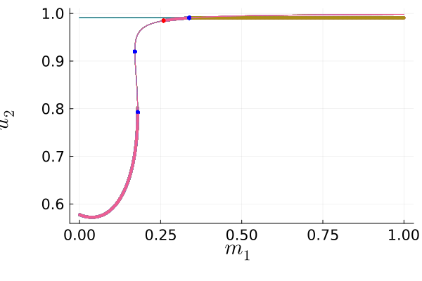
Refer to caption
(a) u1u_{1}
Refer to caption
(b) u2u_{2}
Refer to caption
(c) u3u_{3}
Figure 4: Bifurcation diagram of the three-population-model (6.2). The bifurcation parameter is m1m_{1}. Thin lines indicate unstable states, thick lines stable states. Dots indicate bifurcation points.

Figure 4 shows the bifurcation diagram for the full ODE model (6.2) depending on m1m_{1}. All other parameters are fixed. In the parameter region where none of the stationary states is stable, the system shows oscillations, see Figure 5.

Refer to caption
(a) short time interval
Refer to caption
(b) large time interval
Figure 5: Dynamics of the three-population-model (6.2) for β1\beta_{1} in the unstable region.

The two bifurcation diagrams are relevant for comparing with the reduced ODE system (6.2). In the one prey - one predator system (6.2), we see the change of the system behaviour from stable stationary states for small m1m_{1} to oscillating solution for larger m1m_{1}, see Figure 6. For very small m1m_{1}, only the prey population survives, and the predator population becomes extinct.
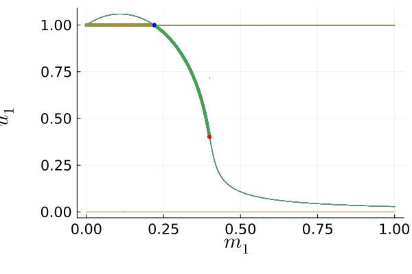
Refer to caption
(a) prey u1u_{1}
Refer to caption
(b) predator u3u_{3}
Figure 6: Bifurcation diagram of the one prey - one predator system (6.2) with the bifurcation parameter m1m_{1}.

The oscillatory behaviour of the predator-prey system for parameter values m1m_{1} larger (or equal) to the red Hopf bifurcation point is shown in Figure 7.

Refer to caption
Figure 7: Oscillatory dynamics of the one prey - one predator system (6.2).

The predator-prey model with only one prey population shows that for small parameters, the predator extinction occurs for small m1m_{1}, then stationary co-existence and the well-known oscillations for larger m1m_{1}.

The two-prey-one-predator model under investigation in this paper shows depending on the parameter m1m_{1} a different behaviour: for small m1m_{1}, all three populations co-exist, for some medium parameter values m1m_{1} the system oscillates, and for large m1m_{1} the system becomes a one-prey-one-predator system due to extinction of u2u_{2}. The oscillations show a time-delay of population maxima of the two prey. Therefore, combining the two prey populations into one prey population is not meaningful and reduces the system’s complexity.

Consequently, the ordinary differential equation setting of the studied model shows a richer behaviour than the two included two-population models. The space-depending system in Figure 1 shows the same behaviour due to a fast levelling of any spatial difference. The study of a chemotaxis system with two prey populations and one predator population is therefore an extension of models for one prey population.

7 Further comments

Our results are obtained for the system with only parabolic equation for v3εv_{3}^{\varepsilon}. However, the analysis clearly works with the fully parabolic system, i.e. the system in which equations for all chemical concentrations are parabolic, given as follows

{∂tu1ε−d1Δu1ε−χ1∇⋅(u1ε∇v3ε)=f1​(u1ε,u2ε,u3ε),∂tu2ε−d2Δu2ε−χ2∇⋅(u2ε∇v3ε)=f2​(u1ε,u2ε,u3ε),∂tu3ε−d3Δu3ε+∑i=12χ3​i∇⋅(u3ε∇viε)=f3​(u1ε,u2ε,u3ε),ε​∂tviε−λi​Δ​viε+μi​viε=ζi​uiε,i=1,2,3,\displaystyle\left\{\begin{array}[]{llll}\hskip 4.26773pt\partial_{t}u_{1}^{\varepsilon}-d_{1}\Delta u_{1}^{\varepsilon}-\chi_{1}\nabla\cdot(u_{1}^{\varepsilon}\nabla v_{3}^{\varepsilon})&\hskip-5.69046pt=&f_{1}(u_{1}^{\varepsilon},u_{2}^{\varepsilon},u_{3}^{\varepsilon}),\\ \hskip 4.26773pt\partial_{t}u_{2}^{\varepsilon}-d_{2}\Delta u_{2}^{\varepsilon}-\chi_{2}\nabla\cdot(u_{2}^{\varepsilon}\nabla v_{3}^{\varepsilon})&\hskip-5.69046pt=&f_{2}(u_{1}^{\varepsilon},u_{2}^{\varepsilon},u_{3}^{\varepsilon}),\\ \hskip 4.26773pt\partial_{t}u_{3}^{\varepsilon}-d_{3}\Delta u_{3}^{\varepsilon}+\sum_{i=1}^{2}\chi_{3i}\nabla\cdot(u_{3}^{\varepsilon}\nabla v_{i}^{\varepsilon})&\hskip-5.69046pt=&f_{3}(u_{1}^{\varepsilon},u_{2}^{\varepsilon},u_{3}^{\varepsilon}),\\ \varepsilon\partial_{t}v_{i}^{\varepsilon}-\lambda_{i}\Delta v_{i}^{\varepsilon}+\mu_{i}v_{i}^{\varepsilon}=\zeta_{i}u_{i}^{\varepsilon},&&i=1,2,3,\end{array}\right.

equipped with the boundary - initial conditions

(∇uiε⋅ν,∇viε⋅ν)|Γ∞=0,(uiε(0),viε(0))|Ω=(ui​0,v30),i=1,2,3.\displaystyle(\nabla u_{i}^{\varepsilon}\cdot\nu,\nabla v_{i}^{\varepsilon}\cdot\nu)|_{\Gamma_{\infty}}=0,\quad(u_{i}^{\varepsilon}(0),v_{i}^{\varepsilon}(0))|_{\Omega}=(u_{i0},v_{30}),\quad i=1,2,3. (136)

In this case, we can see from Theorems 2.1-2.3 the following slight differences

  • •

    The feedback argument from prey to predator as Lemma 3.2 is not necessary for the global existence;

  • •

    The components v1ε,v2ε,v3εv_{1}^{\varepsilon},v_{2}^{\varepsilon},v_{3}^{\varepsilon} are uniformly bounded in L∞​(QT)∩Lq​(0,T,W2,q​(Ω))L^{\infty}(Q_{T})\cap L^{q}(0,T;W^{2,q}(\Omega)); and

  • •

    The L∞L^{\infty}-in-time convergence rates v^1ε,v^2ε,v^3ε\widehat{v}^{\,\varepsilon}_{1},\widehat{v}^{\,\varepsilon}_{2},\widehat{v}^{\,\varepsilon}_{3} will be affected by the initial layer corresponding to the critical manifold

    {(ui​0,vi​0)∈L2(Ω)3×H2(Ω)3:λiΔvi−μivi+ζiui=0,i=1,2,3}.\big\{(u_{i0},v_{i0})\in L^{2}(\Omega)^{3}\times H^{2}(\Omega)^{3}:\,\lambda_{i}\Delta v_{i}-\mu_{i}v_{i}+\zeta_{i}u_{i}=0,i=1,2,3\big\}.

Since our analysis is not restricted to only positive chemotaxis coefficients, fast signal diffusion limits and L∞L^{\infty}-in-time convergence rates for the following two-dimensional chemotaxis system can be studied similarly

{∂tuiε−diΔuiε+∑j=1kχi​j∇⋅(uiε∇vjε)=fi(u1ε,…,ukε),εi​∂tviε−λi​Δ​viε+μi​viε=ζi​uiε,\displaystyle\left\{\begin{array}[]{llll}\partial_{t}u_{i}^{\varepsilon}-d_{i}\Delta u_{i}^{\varepsilon}+\displaystyle\sum_{j=1}^{k}\chi_{ij}\nabla\cdot(u_{i}^{\varepsilon}\nabla v_{j}^{\varepsilon})=f_{i}(u_{1}^{\varepsilon},\dots,u_{k}^{\varepsilon}),\\ \varepsilon_{i}\partial_{t}v_{i}^{\varepsilon}-\lambda_{i}\Delta v_{i}^{\varepsilon}+\mu_{i}v_{i}^{\varepsilon}=\zeta_{i}u_{i}^{\varepsilon},\end{array}\right.

i=1,…,ki=1,\dots,k, which is subjected to the homogeneous Neumann boundary conditions and given smooth initial data. Here, di>0d_{i}>0, χi​j∈ℝ\chi_{ij}\in\mathbb{R}, λi,μi,ζi>0\lambda_{i},\mu_{i},\zeta_{i}>0 for 1≤i,j≤k1\leq i,j\leq k. The parameters ε1,…,εk∈{0;ε}\varepsilon_{1},\dots,\varepsilon_{k}\in\{0;\,\varepsilon\}, with 0<ε≪10<\varepsilon\ll 1, satisfy that there exists at least one different from 00. The species kinetics are generally of the competitive or logistic types.

Acknowledgement

The authors would like to thank Bao Quoc Tang for his valuable comments on the paper and Simon-Christian Klein for discussing the numerical schemes. The second author is funded by the FWF project “Quasi-steady-state approximation for PDE”, number I-5213. The third author is partially supported by NSFC Grants No. 12271227 and China Scholarship Council (Contract No. 202206180025).

Conflict of Interest The authors declare that they have no conflict of interest.

Data Availability Data sharing not applicable.

Appendices

This part is to recall or slightly improve well-known results related to heat semigroup, heat regularisation, and maximal regularity, where we assume that Ω\Omega is a bounded domain in ℝN\mathbb{R}^{N} with sufficiently smooth (such as C2+αC^{2+\alpha} for some α>0\alpha>0) boundary.

Appendix A Neumann heat semigroup

For λ,μ>0\lambda,\mu>0 and 1<p<∞1<p<\infty, the sectorial operator −λ​Δ+μ​I-\lambda\Delta+\mu I defined on {v∈W2,p(Ω):∇v⋅ν=0 on Γ}\{v\in W^{2,p}(\Omega):\nabla v\cdot\nu=0\text{ on }\Gamma\} has a countable sequence of eigenvalues with the smallest one is μ>0\mu>0. Therefore, it generates an analytic semigroup {et⁡(λ​Δ−μ​I)}t≥0\{e^{t(\lambda\Delta-\mu I)}\}_{t\geq 0} on Lp​(Ω)L^{p}(\Omega) such that

‖(λ​Δ−μ​I)β​et⁡(λ​Δ−μ​I)​f‖Lp​(Ω)≤C​e−ω​t​t−β​‖f‖Lp​(Ω),t>0,\displaystyle\|(\lambda\Delta-\mu I)^{\beta}e^{t(\lambda\Delta-\mu I)}f\|_{L^{p}(\Omega)}\leq Ce^{-\omega t}t^{-\beta}\|f\|_{L^{p}(\Omega)},\quad t>0, (137)

for some ω>0\omega>0 and all β≥0\beta\geq 0, see [HW05, Lemma 2.1]. In particular, if β=0\beta=0, we can take ω=μ\omega=\mu and C=1C=1 (i.e. we have a contraction semigroup), see [Ama84, Theorem 13.4]. Note that et⁡(λ​Δ−μ​I)e^{t(\lambda\Delta-\mu I)} is not commutative with the divergence ∇⁣⋅\nabla\cdot. A combination of them is estimated as follows, where, for the purpose of consistency, we will use the same ω\omega not only in Lemma A.1 but also throughout the paper.

Lemma A.1 ([HW05, Lemma 2.1]).

Let 1<p<∞1<p<\infty. Then, for all κ>0\kappa>0,

∥(−λΔ+μI)βet​λ​Δ∇⋅v∥Lp​(Ω)≤Cκe−ω​tt−β−12−κ∥v∥Lp​(Ω),t>0,\displaystyle\|(-\lambda\Delta+\mu I)^{\beta}e^{t\lambda\Delta}\nabla\cdot v\|_{L^{p}(\Omega)}\leq C_{\kappa}e^{-\omega t}t^{-\beta-\frac{1}{2}-\kappa}\|v\|_{L^{p}(\Omega)},\quad t>0,

for some ω>0\omega>0 and all v∈C0∞​(Ω)v\in C_{0}^{\infty}(\Omega), β≥0\beta\geq 0. The operator (−λΔ+μI)ket​λ​Δ∇⋅(-\lambda\Delta+\mu I)^{k}e^{t\lambda\Delta}\nabla\cdot consequently admits an only extension (with the same notation) to the whole space Lp​(Ω)L^{p}(\Omega).

The Neumann heat semigroup {et⁡(λ​Δ−μ​I)}t≥0\{e^{t(\lambda\Delta-\mu I)}\}_{t\geq 0} on Lp​(Ω)L^{p}(\Omega) can also be used in expressing solutions to some elliptic equations. Indeed, let us consider the elliptic problem

−λΔv+μv=f in Ω,and∇v⋅ν=0 on Γ.\displaystyle-\lambda\Delta v+\mu v=f\text{ in }\Omega,\quad\text{and}\quad\nabla v\cdot\nu=0\text{ on }\Gamma. (138)

Since λ,μ>0\lambda,\mu>0, all eigenvalues of the Neumann operator −λ​Δ+μ​I-\lambda\Delta+\mu I are strictly positive, and will be {bi}i≥1\{b_{i}\}_{i\geq 1}, bi:=λ​ai+μb_{i}:=\lambda a_{i}+\mu, if the eigenvalues of the Neumann Laplacian −Δ-\Delta are denoted by {ai}i≥1\{a_{i}\}_{i\geq 1}. We, therefore, can follow from the identity

1bi=∫0∞e−bi​s​𝑑s,for ​λ>0\displaystyle\frac{1}{b_{i}}=\int_{0}^{\infty}e^{-b_{i}s}\,ds,\quad\text{for }\lambda>0 (139)

that

v⁡(x)\displaystyle v(x) =(−λ​Δ+μ​I)−1​f​(x)=(∫0∞es⁡(λ3​Δ−μ​I)​𝑑s)​f​(x).\displaystyle=(-\lambda\Delta+\mu I)^{-1}f(x)=\left(\int_{0}^{\infty}e^{s(\lambda_{3}\Delta-\mu I)}\,ds\right)f(x). (140)

Appendix B Heat regularisation

To obtain optimal regularity of solutions to the heat equation, we recall here the so called heat regularisation, see [LSU88, Theorem 9.1, Chapter IV].

Lemma B.1 (Heat regularisation).

Let T>0T>0, 1<p<∞1<p<\infty. Assume that f∈Lp​(QT)f\in L^{p}(Q_{T}) and v0∈W2−2/p,p​(Ω)v_{0}\in W^{2-2/p,p}(\Omega) with the compatibility condition ∇v0⋅ν=0\nabla v_{0}\cdot\nu=0 on Γ\Gamma. If vv is the weak solution to

∂tv−λΔv+μv=f in QT,∇v⋅ν=0 on ΓT,v(0)=v0 in Ω,\partial_{t}v-\lambda\Delta v+\mu v=f\text{ in }Q_{T},\quad\nabla v\cdot\nu=0\text{ on }\Gamma_{T},\quad v(0)=v_{0}\text{ in }\Omega, (141)

for λ>0\lambda>0, μ≥0\mu\geq 0, then

‖v‖Lq​(QT)+‖∇v‖Lr​(QT)+‖|∂tv|+|Δ​v|‖Lp​(QT)≤C⁡(‖f‖Lp​(ΩT)+‖v0‖W2−2p,p​(Ω)),\displaystyle\|v\|_{L^{q}(Q_{T})}+\|\nabla v\|_{L^{r}(Q_{T})}+\||\partial_{t}v|+|\Delta v|\|_{L^{p}(Q_{T})}\leq C\left(\|f\|_{L^{p}(\Omega_{T})}+\|v_{0}\|_{W^{2-\frac{2}{p},p}(\Omega)}\right),

where

q={(N+2)​pN+2−2​pif ​p<N+22,∈[1,∞)​ arbitraryif ​p=N+22,∞if ​p>N+22,r={(N+2)​pN+2−pif ​p<N+2,∈[1,∞)​ arbitraryif ​p=N+2,∞if ​p>N+2,\displaystyle q=\left\{\begin{array}[]{lllllll}\dfrac{(N+2)p}{N+2-2p}&\text{if }p<\frac{N+2}{2},\\ \in[1,\infty)\text{ arbitrary}&\text{if }p=\frac{N+2}{2},\\ \infty&\text{if }p>\frac{N+2}{2},\end{array}\right.\quad r=\left\{\begin{array}[]{lllllll}\dfrac{(N+2)p}{N+2-p}&\text{if }p<N+2,\\ \in[1,\infty)\text{ arbitrary}&\text{if }p=N+2,\\ \infty&\text{if }p>N+2,\end{array}\right.

and CC depends only on λ,μ,p,N,Ω,T\lambda,\mu,p,N,\Omega,T, and remains bounded for finite values of T>0T>0.

Remark B.1.

In Lemma B.1, the dependence of the constant CC on TT can be removed by applying Theorem 2.3 in [GS91].

Appendix C LpL^{p}-maximal regularity with independent-of-pp constants

In this part, we present LpL^{p}-maximal regularity, where we emphasise that maximal regularity constants do not depend on pp. This independence plays an important role in the analysis of fast signal diffusion limits.

Lemma C.1 (Elliptic maximal regularity).

Let λ,μ>0\lambda,\mu>0, 1<p<∞1<p<\infty, and f∈Lp​(Ω)f\in L^{p}(\Omega). Then the solution to the problem (138) satisfies the following estimate

‖Δ​v‖Lp​(Ω)≤C𝖤𝖬​‖f‖Lp​(Ω),\displaystyle\|\Delta v\|_{L^{p}(\Omega)}\leq C^{\mathsf{EM}}\|f\|_{L^{p}(\Omega)},

where C𝖤𝖬C^{\mathsf{EM}} depends on λ,μ,Ω,N\lambda,\mu,\Omega,N, but not on pp.

Proof.

By the same argument in Remark 2.1, we have v⁡(x)=∫0∞es⁡(λ​Δ−μ​I)​f​(x)​𝑑sv(x)=\int_{0}^{\infty}e^{s(\lambda\Delta-\mu I)}f(x)ds. Taking into account the fact that the heat semigroup associated with the homogeneous Neumann boundary condition is a contraction semigroup on Lp​(Ω)L^{p}(\Omega), we have

‖Δ​v‖Lp​(Ω)\displaystyle\|\Delta v\|_{L^{p}(\Omega)} =‖−1λ​f+μλ​(∫0∞es⁡(λ​Δ−μ​I)​𝑑s)​f‖Lp​(Ω)\displaystyle=\left\|-\frac{1}{\lambda}f+\frac{\mu}{\lambda}\left(\int_{0}^{\infty}e^{s(\lambda\Delta-\mu I)}\,ds\right)f\right\|_{L^{p}(\Omega)}
≤1λ​‖f‖Lp​(Ω)+μλ​(∫0∞e−ω​s​𝑑s)​‖f‖Lp​(Ω),\displaystyle\leq\frac{1}{\lambda}\|f\|_{L^{p}(\Omega)}+\frac{\mu}{\lambda}\left(\int_{0}^{\infty}e^{-\omega s}\,ds\right)\|f\|_{L^{p}(\Omega)},

where the improper integral is finite. ∎

In the following lemma, we improve the heat regularisation given in Lemma B.1 in the sense that the dependence of CC on both TT and pp will be removed.

Lemma C.2.

If vv is the solution to (141) with λ>0\lambda>0, μ≥0\mu\geq 0, then

‖Δ​v‖Lp​(QT)≤Cλ,μ,p0𝖯𝖬​(‖v0‖W2,p​(Ω)+‖f‖Lp​(QT)),2≤p≤p0,\displaystyle\|\Delta v\|_{L^{p}(Q_{T})}\leq C_{\lambda,\mu,p_{0}}^{\mathsf{PM}}\left(\|v_{0}\|_{W^{2,p}(\Omega)}+\|f\|_{L^{p}(Q_{T})}\right),\quad 2\leq p\leq p_{0}, (142)

for p0<∞p_{0}<\infty, where Cλ,μ,p0𝖯𝖬C_{\lambda,\mu,p_{0}}^{\mathsf{PM}} depends on λ,μ,Ω,N\lambda,\mu,\Omega,N, but not on p,Tp,T. Moreover, the constant will be Cλ,μ,p𝖯𝖬C_{\lambda,\mu,p}^{\mathsf{PM}}, i.e. it generally depends on pp if we consider 1<p<∞1<p<\infty.

Proof.

We split vv into the sum of v~\widetilde{v} and v^\widehat{v}, which are the solutions in the cases v0=0v_{0}=0 and f=0f=0, respectively. Thanks to Lemma [Lam87, Theorem 1], there exists an optimal constant Cλ,μ,pC_{\lambda,\mu,p}, which may depend on Ω,N\Omega,N but not on TT, such that

‖Δ​v~‖Lp​(QT)≤Cλ,μ,p​‖f‖Lp​(QT).\displaystyle\|\Delta\widetilde{v}\|_{L^{p}(Q_{T})}\leq C_{\lambda,\mu,p}\|f\|_{L^{p}(Q_{T})}. (143)

On the other hand, it is straightforward to see Cλ,μ,2≤1/λC_{\lambda,\mu,2}\leq 1/\lambda due to multiplying the equation for v~\widetilde{v} by −Δ​v~-\Delta\widetilde{v}. Specifically, we have

‖Δ​v~‖L2​(QT)≤1λ​‖f‖L2​(QT).\displaystyle\|\Delta\widetilde{v}\|_{L^{2}(Q_{T})}\leq\frac{1}{\lambda}\|f\|_{L^{2}(Q_{T})}. (144)

Let us use the same idea in [CDF14, Lemma 3.2] with an interpolation between (143) for p=p0p=p_{0} and (144), which gives Cλ,μ,p≤λ−s​(Cλ,μ,p0)1−sC_{\lambda,\mu,p}\leq\lambda^{-s}(C_{\lambda,\mu,p_{0}})^{1-s}, 1/p=s/2+(1−s)/p01/p=s/2+(1-s)/p_{0}. We get

Cλ,μ,p≤λ2p0−2​(1−p0p)​(Cλ,μ,p0)p0p0−2​(1−2p)≤max⁡(1,Cλ,μ,p0)min⁡(1,λ).\displaystyle C_{\lambda,\mu,p}\leq\lambda^{\frac{2}{p_{0}-2}(1-\frac{p_{0}}{p})}(C_{\lambda,\mu,p_{0}})^{\frac{p_{0}}{p_{0}-2}(1-\frac{2}{p})}\leq\frac{\max(1;C_{\lambda,\mu,p_{0}})}{\min(1;\lambda)}.

On the other hand, by the estimate (137),

‖Δ​v^‖Lp​(QT)=‖et⁡(λ​Δ−μ​I)​Δ​v0‖Lp​(QT)≤‖Δ​v0‖Lp​(QT).\displaystyle\|\Delta\widehat{v}\|_{L^{p}(Q_{T})}=\|e^{t(\lambda\Delta-\mu I)}\Delta v_{0}\|_{L^{p}(Q_{T})}\leq\|\Delta v_{0}\|_{L^{p}(Q_{T})}. (145)

We obtain the estimate (142) by combining (143) and (145), where

Cλ,μ,p0𝖯𝖬:=1+max⁡(1,Cλ,μ,p0)min⁡(1,λ).\displaystyle C_{\lambda,\mu,p_{0}}^{\mathsf{PM}}:=1+\frac{\max(1;C_{\lambda,\mu,p_{0}})}{\min(1;\lambda)}.

The conclusion for the case 1<p<∞1<p<\infty is clear without the use of the interpolation. ∎

References

  • [ABOV23] Paulo Amorim, Raimund Bürger, Rafael Ordoñez, and Luis Miguel Villada. Global existence in a food chain model consisting of two competitive preys, one predator and chemotaxis. Nonlinear Analysis: Real World Applications, 69:103703, 2023.
  • [Ama84] Herbert Amann. Existence and regularity for semilinear parabolic evolution equations. Annali della Scuola Normale Superiore di Pisa-Classe di Scienze, 11(4):593–676, 1984.
  • [Bal04] John M Ball. Global attractors for damped semilinear wave equations. Discrete and Continuous Dynamical Systems, 10(1/2):31–52, 2004.
  • [Bla17] Tobias Black. Global existence and asymptotic stability in a competitive two-species chemotaxis system with two signals. Discrete & Continuous Dynamical Systems-Series B, 22(4), 2017.
  • [BOSV20] Raimund Bürger, Rafael Ordoñez, Mauricio Sepúlveda, and Luis Miguel Villada. Numerical analysis of a three-species chemotaxis model. Computers & Mathematics with Applications, 80(1):183–203, 2020.
  • [Bre11] Haim Brezis. Functional analysis, Sobolev spaces and partial differential equations, volume 2, Number 3. Springer, 2011.
  • [CDF14] José A Canizo, Laurent Desvillettes, and Klemens Fellner. Improved duality estimates and applications to reaction-diffusion equations. Communications in Partial Differential Equations, 39(6):1185–1204, 2014.
  • [CHVY19] José A Carrillo, Sabine Hittmeir, Bruno Volzone, and Yao Yao. Nonlinear aggregation-diffusion equations: radial symmetry and long time asymptotics. Inventiones Mathematicae, 218:889–977, 2019.
  • [CPZ04] Lucilla Corrias, Benoît Perthame, and Hatem Zaag. Global solutions of some chemotaxis and angiogenesis systems in high space dimensions. Milan Journal of Mathematics, 72:1–28, 2004.
  • [Day41] Mahlon M Day. Some more uniformly convex spaces. Bulletin of the American Mathematical Society, 47:504–507, 1941.
  • [Fre20] Marcel Freitag. The fast signal diffusion limit in nonlinear chemotaxis systems. Discrete & Continuous Dynamical Systems-Series B, 25(3), 2020.
  • [GNU24] S Gnanasekaran, N Nithyadevi, and C Udhayashankar. Global existence and asymptotic behavior of a predator–prey chemotaxis system with inter-species interaction coefficients. Journal of Differential Equations, 378:264–302, 2024.
  • [GS91] Yoshikazu Giga and Hermann Sohr. Abstract LpL^{p} estimates for the cauchy problem with applications to the Navier-Stokes equations in exterior domains. Journal of Functional Analysis, 102(1):72–94, 1991.
  • [Hen06] Daniel Henry. Geometric theory of semilinear parabolic equations, volume 840. Springer, 2006.
  • [HT16] Felix Henneke and Bao Q Tang. Fast reaction limit of a volume–surface reaction–diffusion system towards a heat equation with dynamical boundary conditions. Asymptotic Analysis, 98(4):325–339, 2016.
  • [HW05] Dirk Horstmann and Michael Winkler. Boundedness vs. blow-up in a chemotaxis system. Journal of Differential Equations, 215(1):52–107, 2005.
  • [JL92] Willi Jäger and Stephan Luckhaus. On explosions of solutions to a system of partial differential equations modelling chemotaxis. Transactions of the American Mathematical Society, 329(2):819–824, 1992.
  • [KNRY22] Alexander Kiselev, Fedor Nazarov, Lenya Ryzhik, and Yao Yao. Chemotaxis and reactions in biology. Journal of the European Mathematical Society, 25(7):2641–2696, 2022.
  • [KO20] Masaki Kurokiba and Takayoshi Ogawa. Singular limit problem for the two-dimensional Keller-Segel system in scaling critical space. Journal of Differential Equations, 269(10):8959–8997, 2020.
  • [KR12] Alexander Kiselev and Lenya Ryzhik. Biomixing by chemotaxis and enhancement of biological reactions. Communications in Partial Differential Equations, 37(2):298–318, 2012.
  • [Lam87] Damien Lamberton. Equations d’évolution linéaires associées a des semi-groupes de contractions dans les espaces Lp{L}^{p}. Journal of Functional Analysis, 72(2):252–262, 1987.
  • [LSU88] Ol’ga A Ladyženskaja, Vsevolod Alekseevich Solonnikov, and Nina N Ural’ceva. Linear and quasi-linear equations of parabolic type, volume 23. American Mathematical Soc., 1988.
  • [LX21] Min Li and Zhaoyin Xiang. The convergence rate of the fast signal diffusion limit for a Keller–Segel–Stokes system with large initial data. Proceedings of the Royal Society of Edinburgh Section A: Mathematics, 151(6):1972–2012, 2021.
  • [LX23] Min Li and Zhaoyin Xiang. Convergence analysis from the indirect signal production to the direct one. Journal of Differential Equations, 367:834–889, 2023.
  • [LXZ23] Min Li, Zhaoyin Xiang, and Guanyu Zhou. The stability analysis of a 2D Keller–Segel–Navier–Stokes system in fast signal diffusion. European Journal of Applied Mathematics, 34(1):160–209, 2023.
  • [Miz18] Masaaki Mizukami. The fast signal diffusion limit in a chemotaxis system with strong signal sensitivity. Mathematische Nachrichten, 291(8-9):1342–1355, 2018.
  • [Miz19] Masaaki Mizukami. The fast signal diffusion limit in a Keller–Segel system. Journal of Mathematical Analysis and Applications, 472(2):1313–1330, 2019.
  • [MO23] Alexis Montoison and Dominique Orban. Krylov.jl: A Julia basket of hand-picked Krylov methods. Journal of Open Source Software, 8(89):5187, 2023.
  • [MS14] Noriko Mizoguchi and Philippe Souplet. Nondegeneracy of blow-up points for the parabolic Keller–Segel system. In Annales de l’IHP Analyse Non Linéaire, volume 31, pages 851–875, 2014.
  • [OS23] Takayoshi Ogawa and Takeshi Suguro. Maximal regularity of the heat evolution equation on spatial local spaces and application to a singular limit problem of the Keller–Segel system. Mathematische Annalen, 387(1-2):389–431, 2023.
  • [PWZW20] Xu Pan, Liangchen Wang, Jing Zhang, and Jie Wang. Boundedness in a three-dimensional two-species chemotaxis system with two chemicals. Zeitschrift für Angewandte Mathematik und Physik, 71(1):26, 2020.
  • [RN17] Christopher Rackauckas and Qing Nie. DifferentialEquations.jl–a performant and feature-rich ecosystem for solving differential equations in Julia. Journal of Open Research Software, 5(1), 2017.
  • [TT24] Bao Quoc Tang and Bao-Ngoc Tran. Rigorous derivation of Michaelis-Menten kinetics in the presence of slow diffusion. SIAM J. Math. Anal., Vol. 56, Iss. 5, 2024.
  • [TTQ21] Xinyu Tu, Chun-Lei Tang, and Shuyan Qiu. The phenomenon of large population densities in a chemotaxis competition system with loop. Journal of Evolution Equations, 21:1717–1754, 2021.
  • [TW15] Youshan Tao and Michael Winkler. Boundedness vs. blow-up in a two-species chemotaxis system with two chemicals. Discrete Contin. Dyn. Syst. Ser. B, 20(9):3165–3183, 2015.
  • [Vel20] Romain Veltz. BifurcationKit.jl, July 2020.
  • [WHZ25] Jianwang Wu, Yinuo Han, and Qian Zhang. On the fast signal limit in a chemotaxis system involving a tensor-valued sensitivity. Authorea Preprints, 2025.
  • [Win10] Michael Winkler. Boundedness in the higher-dimensional parabolic-parabolic chemotaxis system with logistic source. Communications in Partial Differential Equations, 35(8):1516–1537, 2010.
  • [WWX19] Yulan Wang, Michael Winkler, and Zhaoyin Xiang. The fast signal diffusion limit in Keller–Segel (-fluid) systems. Calculus of Variations and Partial Differential Equations, 58(6):196, 2019.
  • [YTY22] Hongying Yang, Xinyu Tu, and Li Yang. Global solvability and asymptotic behaviour in a two-species chemotaxis system with two chemicals. Mathematical Methods in the Applied Sciences, 45(12):7663–7684, 2022.
  • [ZM17] Pan Zheng and Chunlai Mu. Global boundedness in a two-competing-species chemotaxis system with two chemicals. Acta Applicandae Mathematicae, 148:157–177, 2017.