Towards Transparent and Efficient Anomaly Detection in Industrial Processes through ExIFFI

Abstract

Anomaly Detection (AD) is crucial in industrial settings to streamline operations by detecting underlying issues. Conventional methods merely label observations as normal or anomalous, lacking crucial insights. In Industry 5.0, interpretable outcomes become desirable to enable users to understand the rationale behind model decisions. This paper presents the first industrial application of ExIFFI, a recent approach for fast, efficient explanations for the Extended Isolation Forest (EIF) AD method. ExIFFI is tested on four industrial datasets, demonstrating superior explanation effectiveness, computational efficiency and improved raw anomaly detection performances. ExIFFI reaches over 90% of average precision on the benchmarks considered in the study and outperforms state-of-the-art Explainable Artificial Intelligence (XAI) approaches in terms of the feature selection proxy task metric which was specifically introduced to quantitatively evaluate model explanations.

Keywords Anomaly Detection, Explainable Artificial Intelligence, Industrial Internet of Things

1 Introduction

The rapid expansion of Machine Learning (ML) has driven advances in Internet of Things (IoT) technologies, enabling widespread deployment of interconnected sensor networks [19]. This is particularly relevant in Industrial Internet of Things (IIoT), which focuses on real-time monitoring of industrial assets to optimize maintenance and production efficiency [29]. As IoT systems generate vast datasets, ML plays a key role in extracting predictive insights, reflecting the symbiotic relationship between ML and IIoT [4].

A key application within this context is unsupervised AD [15], especially prominent in settings where labeling data is impractical. Among AD methods, models based on Isolation Forest (IF) [23], in particular EIF [21] stands out due to its speed, low memory requirements, and high performance, making it well-suited for industrial AD [5]. However, detecting anomalies alone is insufficient; identifying their root causes is equally important [9]. XAI addresses this by making EIF outputs interpretable, supporting informed decision-making in IIoT environments [2].

This paper specifically evaluates the Extended Isolation Forest Feature Importance (ExIFFI) algorithm, developed by Arcudi et al. [3], which provides a time-efficient and tailored interpretative approach to the EIF model. Moreover, [3] introduces a modification of EIF named $\text{EIF}^{+}$, which improves generalization and is also interpretable by ExIFFI.

This paper extends [18] with additional and more robust experimental results on the applicability of EIF, $\text{EIF}^{+}$, and ExIFFI in industrial environments. Specifically, the contributions are:

• An evaluation of the explained models in terms of AD performances, detailed in 4.3.

• ExIFFI performance assessment for Packaging Industry Anomaly DEtection (PIADE) is extended to all five machines in the study, as presented in 4.5.1.

• The effect of hyperparameters such as number of trees and contamination factor on ExIFFI is assessed via ablation studies in 4.10.

• The addition of two new benchmark dataset, CoffeeData and Service Machine Data (SMD), introduced in 4.1.2 and 4.1.1.

• Additional experiments on two synthetic datasets to showcase key theoretical properties of multivariate feature importance of ExIFFI in 4.9.

• Additional images to showcase the results of Feature Selection (Figures 4.4.2, 4.6.2).

• Inference experiments on a Raspberry PI 3 Model B to assess the industrial applicability of ExIFFI in resource constrained environments 4.8.

The paper is organized as follows: Section 2 contextualizes ExIFFI within Industry 5.0; Section 3 describes the algorithm; Section 4 presents benchmark datasets and results. Properties of ExIFFI are further analyzed via synthetic datasets (4.9) and ablation studies (4.10). Sections 5 and 6 discuss limitations, findings, and future directions.

2 Related Work

The transition from Industry 4.0 [22] to Industry 5.0 [34] shifts the focus from automation-driven performance to human-centric outcomes [41], integrating human creativity with Artificial Intelligence (AI) and robotics while requiring transparency and interpretability in ML models.

This need is addressed by implementing XAI in industrial applications, including fault detection in machinery [6], process monitoring across sectors from semiconductors to home appliances [10, 17, 8], and predictive maintenance [35]. ExIFFI exemplifies this trend, offering fast and precise interpretation of EIF-based AD models for IIoT environments.

Recent works on XAI for Deep Learning (DL) in industrial AD, proposed transformer-based architectures for multi-sensor systems [12, 13], graph neural networks for IT infrastructure monitoring [42], and deep SVDD variants [37]. Post-hoc XAI methods like SHapley Additive exPlanations (SHAP) have also been applied to DL approaches for various domains [28, 31].

However, DL methods often require large training datasets and computational resources, labeled anomalies [37], and their interpretability can be limited compared to methods specifically designed for XAI. This study focuses on an unsupervised and lightweight approach that is easier to integrate in resource-constrained industrial systems. In particular, the EIF algorithm was considered due to its excellent performance in the AD benchmarks [20].

We evaluate ExIFFI against various XAI techniques, including model-specific interpretability, i.e., one that exploits the inner working of a particular algorithm, like Depth Based Isolation Forest Feature Importance (DIFFI) [11] which is tailored for the Isolation Forest; and model-agnostic methods that instead are independent of the underlying model [25] such as KernelSHAP [24] and Accelerated Model Explanations for Anomaly Detection (AcME-AD) [38, 39].

KernelSHAP approximates SHAP values for any model but is computationally demanding for large datasets. AcME-AD reduces this cost, making it faster than KernelSHAP while remaining model-agnostic.

3 Proposed Approach

ExIFFI leverages the structure of the EIF forest, similarly to how DIFFI exploits IF, to assess the contribution of each feature in determining whether a sample is anomalous. Consequently, ExIFFI acts as a post-hoc interpretability wrapper for EIF and $\text{EIF}^{+}$, leaving the underlying model and its AD performance unchanged. Importance scores are computed jointly with model fitting.

Note that, as in IF, the EIF method hypothesizes that anomalous samples are located in low density regions of the input space and thus are simpler to isolate from inliers. Consequently, the algorithm focuses on identifying isolated anomalies and is less suited to identify subtle variations within dense clusters such as [36].

In EIF, each tree $t$ of the forest $\mathcal{T}$ consists of nodes that partition the space using a hyperplane $\mathcal{H}_{k}^{t}$. Each hyperplane is defined by a normal vector $\mathbf{v}_{k}^{t}$ and an intercept point $\mathbf{p}^{t}_{k}$. The hyperplane splits the data sample $X_{k}^{t}$ into two distinct subsets $L^{t}_{k}$ and $R^{t}_{k}$, with $L^{t}_{k}\cup R^{t}_{k}=X_{k}^{t}$ and $L^{t}_{k}\cap R^{t}_{k}=\varnothing$. ExIFFI assesses the feature importance by calculating the imbalance generated by each node for a given sample $x$ as follows:

$$\mathbf{\lambda}^{t}_{k}(\mathbf{x})=\begin{cases}\left(\frac{|X^{t}_{k}|}{|L^{t}_{k}|}\right)\text{abs}(\mathbf{v}^{t}_{k}),&\text{if }\mathbf{v}^{t}_{k}\cdot\mathbf{x}>\mathbf{v}^{t}_{k}\cdot\mathbf{p}^{t}_{k}\\ \left(\frac{|X^{t}_{k}|}{|R^{t}_{k}|}\right)\text{abs}(\mathbf{v}^{t}_{k}),&\text{otherwise}\end{cases}$$ (1)

Differently from IF, the non axis-aligned hyperplanes of EIF help to better detect anomalies spread along multiple dimensions, avoiding the IF [5] structural biases [21]. Consequently explainability is enhanced even in highly dimensional datasets with importance scores naturally distributed among multiple important features, as demonstrated in Section 4.9.

The feature importance for a sample $x$ within a specific tree $t$ is determined by summing the importance vectors from all nodes $k$ that $x$ traverses on its path to the leaf, and the overall importance across the entire forest is obtained by aggregating over all trees:

$$\mathbf{I}_{t}(x)=\sum_{k\in\mathcal{P}^{t}_{x}}\mathbf{\lambda}_{k}^{t}(x),\qquad\mathbf{I}(x)=\sum_{t\in\mathcal{T}}\mathbf{I}_{t}(x)$$ (2)

$\mathbf{I}(x)$ quantifies each feature’s contribution to the isolation of $x$. To correct for biases caused by features being sampled more frequently, $\mathbf{I}(x)$ is normalized by the sum of vectors orthogonal to the hyperplanes of the nodes that $x$ traverses in each tree:

$$\mathbf{V}(x)=\sum_{t\in\mathcal{T}}\sum_{k\in\mathcal{P}^{t}}\mathbf{v}_{k}^{t},\qquad\mathbf{LFI}(x)=\frac{\mathbf{I}(x)}{\mathbf{V}(x)}$$ (3)

The resulting Local Feature Importance (LFI) score identifies which features most influence the classification of $x$ as anomalous, enabling targeted root cause analysis. Grouping together the importance vectors assigned to all samples, ExIFFI also provides a Global Feature Importance (GFI), a single vector quantifying the overall importance of each feature in discriminating between inliers and outliers:

$$\mathbf{GFI}=\frac{\hat{\mathbf{I}}_{O}}{\hat{\mathbf{I}}_{I}}$$ (4)

where $\hat{\mathbf{I}}_{O}$ and $\hat{\mathbf{I}}_{I}$ are the importance vectors computed over the set of outliers and inliers respectively.

For what concerns the practical applications of ExIFFI   it can be integrated into a Machine Learning Operations (MLOps) pipeline, enabling automatic visualization of fault root causes, accelerating response to potentially disruptive events.

Domain experts can validate explanations or correct misidentified root causes, which is especially important in unlabeled settings such as PIADE (Section 4.1), as detailed in [18] were GFI ranking results were validated by the opinion of experienced machine’s operators.

4 Experimental Results

This section presents the results of applying ExIFFI to three publicly accessible and a private dataset derived from industrial processes, which serve as benchmarks for evaluating ExIFFI’s effectiveness within real-world contexts. The datasets include Tennessee Eastman Process (TEP), which offers synthetic data with established ground truth for anomaly-inducing features [26], PIADE, which encapsulates typical real-world challenges such as unlabeled and high-dimensional data [33]. SMD [30], instead, contains service logs recorded by a large internet company and is equipped with anomaly labels and ground truth knowledge on anomalies’ root causes. Finally, CoffeeData is a confidential dataset containing sensor measurements recorded during the brewing phase of capsules on coffee machines.

The section is organized as follows: firstly, datasets are presented in 4.1, the experimental setup is provided in 4.2, AD model performances are reported in 4.3, global interpretability is assessed in 4.4.1, 4.6.1 respectively, and four different interpretability models are compared in 4.4.2, 4.6.2 by means of the Feature Selection Proxy Task.

The outcomes here discussed are achieved using Python as the base language to implement the method and C to optimize functions embedded within the performance-critical segments of the Python code.

4.1 Industrial IoT datasets

Below we describe the four benchmark datasets (TEP, PIADE, SMD, and CoffeeData) and their key characteristics.

PIADE consists of machine alarms and statuses, while TEP, SMD, and CoffeeData are time-series datasets. PIADE, SMD, and CoffeeData are collected from real machines, while TEP is simulation-based.

Table 1: The main characteristics of the industrial datasets used for this study are reported: dataset size, sampling rate, source and presence of labels

Dataset	Samples	Features	Sampling Period $[s]$	Anomaly Labels	Source
PIADE	23376	165	3600	No	[33]
TEP	35600	52	180	Yes	[26]
SMD	56956	38	60	Yes	[30]
CoffeeData D1	372	15	0.5	Yes	confidential
CoffeeData D2	255	15	0.5	Yes	confidential

A summary of the main datasets characteristics is reported in Table 1.

We analyze pairwise dependencies among sensor features using both Pearson correlation and mutual information. For example in TEP approximately 41% of feature pairs exhibit negligible linear correlation ($|\rho|<0.05$), a large majority (89%) shows non-zero mutual information. Notably, 31% of feature pairs combine near-zero correlation with positive mutual information, indicating substantial nonlinear dependencies among sensor measurements, a challenging aspect for root cause analysis.

For a more detailed description of the TEP and PIADE datasets please refer to [18].

4.1.1 SMD Dataset

The SMD dataset is a publicly available multivariate time series dataset introduced in [30]. The data were collected over a period of 5 weeks by a large Internet company, encompassing 28 distinct service machines organized into three entity groups. Each machine’s data is split into two halves: the first is used for training and the second for testing. Following the original dataset configuration, each machine constitutes a separate and independent dataset. For this study, we focus exclusively on the machine-1-1 subset.

Anomalies in this dataset occur as contiguous time intervals rather than isolated points, posing a challenge for isolation-based methods (Section 5).

4.1.2 CoffeeData Dataset

The CoffeeData dataset was firstly introduced in [32]. It is a confidential dataset and consists of multiple time-series representing the brewing process of capsules in coffee machines. The goal is to detect anomalous capsule usages early to improve brewing quality. Anomalous behaviors include using the same capsule twice or more times (i.e. reused capsule) or using the coffee machine without any capsule inside it (i.e. no capsule).

Following the procedure introduced in [32], only the water flow rate signal was considered, as it was the most informative one.

Each time series is trimmed to the first 15 samples of the pre-infusion phase, as this segment provides enough information to address the problem effectively while also allowing for early detection of anomalies, which is critical for practical use.

Rather than hand-crafted features as in [32], raw time samples are used directly, with timestamps as features ranked by ExIFFI. This allows identifying the time instants at which anomalies occur, enabling early alarm triggering for improper equipment usage.

Table 2 outlines the dataset composition: standard capsules are part of the inliers group (comprising both original and compatible brands), while there are two kinds of anomalous samples: reused capsules and no capsules.

Table 2: CoffeeData dataset composition.

Brewing	Capsule	# Samples	Class
1st	standard	71	Normal
2nd	standard	229
any	reused capsule	78	Anomaly
	no capsule	26

Normal capsules are divided into the first and second brewings categories as defined in [32].

Second-brewing trials require no cool-down and are thus more frequent, resulting in a higher sample count.

4.2 Experimental Setup

To assess ExIFFI both qualitatively and quantitatively, three types of experiments are conducted:

• Global Importance Assessment: This experiment produces a Score Plot ranking the features in decreasing order of GFI score. It represents a powerful tool for human operators to discover the root causes of anomalies and take preventive actions.

• Local Scoremaps: Local scoremaps focus on local interpretability by selecting a pair of features and showing how inliers and outliers are distributed along them. An heatmap is superimposed to showcase the distribution of the LFI scores in the feature space.

• Feature Selection Proxy Task: In this study feature selection is used as a proxy task to provide a quantitative measure of the effectiveness of a XAI approach by plotting the trend of the average precision metric as features are progressively removed in increasing or decreasing order of GFI scores.

To account for stochasticity, all experiments are repeated with multiple random seeds to ensure statistical robustness.

For the sake of space results on the Local Scoremaps experiments are not included in this extension. The interested reader can find a detailed analysis of local interpretability in [18].

4.3 AD Performance Comparison

In this section IF, EIF and $\text{EIF}^{+}$ AD models are compared with typical AD metrics for the labeled datasets (i.e. TEP and CoffeeData). Tables 3, 4 report the test set metrics. This evaluation is a crucial step for the application of XAI methods like ExIFFI since their effectiveness highly relies on the accuracy of the explained model.

Table 3: TEP dataset AD metrics for the considered models. Best performance for each metric in bold.

Model	Average Precision	Precision	ROC AUC	Fit Time [s]	Predict Time [s]
IF	0.85	0.90	0.92	1.04	6.00e-5
EIF	0.93	0.90	0.95	0.93	7.00e-5
$\text{EIF}^{+}$	0.93	0.91	0.95	1.22	6.00e-5
AutoEncoder	0.92	0.94	0.95	8.83	2.00e-5
DeepSVDD	0.79	0.87	0.89	1.66	1.00e-6

Table 3 shows how EIF and $\text{EIF}^{+}$ perform better than IF thanks to their higher-complexity data partitioning scheme, leveraging multidimensional splits as opposed to IF.

The fit and predict times of EIF and $\text{EIF}^{+}$ are higher than IF because they simultaneously accumulate importance scores during training. However, this design choice yields a significant benefit at inference time: the importance scores are directly available without requiring an additional explanation phase. As reported in Table 8, this results in substantially lower explanation times for the proposed approach compared to model-agnostic methods.

Two DL-based AD models are also considered for comparison: AutoEncoder [1] and DeepSVDD [27]. While the AutoEncoder achieves slightly higher average precision and ROC AUC scores than $\text{EIF}^{+}$, it requires substantially longer training times, rendering it impractical for time-sensitive industrial applications.

CoffeeData comprises two evaluation datasets: D1, which contains both first and second brewings and both kinds of anomalies (i.e. no capsule and reused capsule); while D2 is more limited, but equivalent to the one used in previous work [32] (i.e. only second brewing data and no capsule anomalies).

Table 4: CoffeeData dataset AD metrics for the considered models. Best performance for each metric in bold.

Dataset	Model	Average Precision	Precision	ROC AUC	Fit Time [s]	Predict Time [s]
D1	IF	0.74	0.65	0.63	1.18	5.48e-5
	EIF	0.77	0.66	0.63	0.81	3.65e-5
	$\text{EIF}^{+}$	0.79	0.65	0.64	0.99	4.87e-5
	AutoEncoder	0.44	0.43	0.62	0.36	3.0e-05
	DeepSVDD	0.34	0.33	0.55	0.13	3.0e-05
D2	IF	0.91	0.96	0.97	0.96	3.04e-5
	EIF	0.97	0.89	0.98	0.74	5.48e-5
	$\text{EIF}^{+}$	0.99	0.96	0.99	0.96	4.26e-5
	AutoEncoder	0.76	0.36	0.87	0.32	4e-05
	DeepSVDD	0.84	0.72	0.91	0.23	3e-05

AD model performances are showcased in Table 4. The increased difficulty associated with D1 translates in slightly worse AD metrics, but still the best performing model is $\text{EIF}^{+}$ followed by EIF and IF. D2 metrics match those in [32], despite using raw time samples instead of hand-crafted features.

It is worth noting that the two DL-based models achieve significantly lower performance than the isolation-based detectors. In particular, AutoEncoder and SVDD struggle on small datasets such as CoffeeData, likely due to their large model capacity and corresponding data requirements. This confirms that these models are not well-suited for industrial settings with limited data availability.

The shorter execution times of AutoEncoder and DeepSVDD on CoffeeData are due to its limited size (comparable to the bootstrap size $\psi=256$ used in ensemble models). However, as shown in Tables 3 and 5, deep learning-based models become significantly less efficient as data size increases.

Table 5: SMD dataset AD metrics for the considered models. Best performance for each metric in bold.

Model	Average Precision	Precision	ROC AUC	Fit Time [s]	Predict Time [s]
IF	0.36	0.39	0.64	0.79	5.00e-5
EIF	0.54	0.61	0.74	0.65	6.00e-5
$\text{EIF}^{+}$	0.55	0.62	0.75	1.02	5.00e-5
AutoEncoder	0.64	0.63	0.80	8.03	2.00e-5
DeepSVDD	0.52	0.60	0.73	1.84	1.00e-6

Given the temporal clustering of anomalies characteristic of SMD (Section 4.1.1) and the dataset’s substantial size, DL-based detectors achieve superior detection performance. Nevertheless, this comes at the cost of significantly higher computational requirements. During inference, however, their execution time is lower with the respect to ensemble methods, as they do not need to aggregate predictions from multiple ensemble components.

Overall, EIF and $\text{EIF}^{+}$ outperform IF by several percentage points across all AD metrics. The ensemble-based models considered in the benchmark provide excellent detection performances and are characterized by fast computational times, making them suitable for industrial applications as showcased in Section 4.8. On the other hand, the DL-based AutoEncoder and DeepSVDD models, although they overperform ensemble-based models on large-scale datasets, are highly inefficient in terms of both fitting and importance computation times and thus impractical for industrial applications.

4.4 Case Study I: TEP Dataset

4.4.1 Global Feature Importance

Figure 1 exhibits the Score Plot for the TEP dataset. Features xmeas_22 and xmeas_11 emerge as more relevant than others, aligning with the ground truth [16] since xmeas_11 is the root cause for fault IDV12. Furthermore, the Sign Directed Graph in [16] proves also the saliency of xmeas_22 (i.e. the Separator cooling water outler temperature), a direct consequence of xmeas_11. The causal relationship between these two attributes leads the model to position them on top of the GFI ranking.

Figure 1: This plot represents the top 8 features of the GFI ranking returned by ExIFFI on TEP.

4.4.2 Feature Selection Proxy Task

Utilizing labelled samples, different XAI models are quantitatively compared on the TEP dataset via the Feature Selection proxy task, described in [3]. Two model-specific approaches (i.e. DIFFI [11] and ExIFFI) are considered alongside two model-agnostic algorithms: AcME-AD [38] and KernelSHAP [24].

All the models were employed to explain the $\text{EIF}^{+}$ AD model, except for DIFFI, tailored to the IF model. As described in 4.2 the proxy task requires producing a GFI ranking. However, AcME-AD and KernelSHAP algorithms can only produce LFI scores, so those are used for their rankings .

Feature Selection plots are grouped in Figure 2(a). Comparing the $AUC_{FS}$ scores, the most effective explanations are produced by ExIFFI and AcME-AD. In these plots, the direct approach has a clearer decreasing trend compared to DIFFI and KernelSHAP, resulting in higher $AUC_{FS}$ values. KernelSHAP struggles to rank features effectively, due to the limitations imposed by the sub-sampled background data to make it computationally feasible, leading to a negative $AUC_{FS}$ score.

Feature Selection plots for the model-agnostic methods AcME-AD and KernelSHAP were produced also considering the IF model achieving similar results .

Moreover the standard deviation of the average precision values is in the order of $10^{-3}$ confirming the statistical significance of the results.

These results further confirm the improvement brought by ExIFFI, and consequently by EIF-based approaches, over the other interpretability methods considered in this study.

((a)) TEP dataset

((b)) CoffeeData dataset

Figure 2: Feature selection results for inverse (red), direct (blue), and random (green) approaches using DIFFI, AcME-AD, KernelSHAP, and ExIFFI XAI: (a) TEP, (b) CoffeeData.

4.5 Case Study II: PIADE Dataset

For the second case study, the PIADE dataset is considered. Differently from TEP, comprising synthetically generated data, PIADE incorporates alarm logs data coming from operating packaging machines lacking annotated samples. Consequently, the application of the Feature Selection proxy task is precluded, confining the experimental results to the assessment of Global interpretability, as addressed in Sections 4.5.1.

4.5.1 Global Feature Importance

This section reports the GFI scores produced by ExIFFI on PIADE. Only a subset of results is reported; full results are in [18].

Table 6: Top three features according to the GFI rankings produced in the different PIADE machines datasets

Dataset	$1^{st}$	$2^{nd}$	$3^{rd}$
piade_s1	%idle	A_066	%scheduled_downtime
piade_s2	%scheduled_downtime	A_010	A_005
piade_s3	%idle	%downtime	A_008
piade_s4	idle/idle	%idle	A_010
piade_s5	%idle	idle/idle	A_005

Table 6 reports the top 3 features obtained from the rankings induced by GFI scores computed on the data from the 5 packaging machines included in PIADE. Taking into account that these machines are of the same type but are inserted in different working and environmental conditions the result show an high consistency in detecting features regarding idle and downtime intervals as important descriptors. On the other hand the differences in the operational environment of the machines introduces some variability in the specific alarm features included in the top 3 rankings.

4.6 Case Study III: CoffeeData Dataset

This section reports results on CoffeeData, which differs from the other datasets due to the time-dependent nature of its data.

4.6.1 Global Feature Importance

Global interpretability on CoffeeData is shown via a visualization designed to highlight the temporal structure of the data.

The top half of Figure 3 reports the average time series divided into normal and anomalous data. In the bottom, the distribution of the GFI scores across multiple runs of each feature is represented with a box-plot, with the median highlighted by an orange line, which shows the time evolution of importance scores.

Figure 3: The trend of the GFI scores increases in the time interval where there is the most significant difference between the time series of normal and anomalous capsules

Analyzing the GFI plot, a significant increase in the importance score can be observed between sample 8 and sample 11, which correspond to the highest difference between normal and anomalous time series, as observable in 3. This result confirms the ability of the ExIFFI interpretation to identify a good moment to signal the user about an anomalous usage of the equipment.

4.6.2 Feature Selection Proxy Task

Figure 2(b) depicts the Feature Selection plots for the four interpretations under analysis. The plot is produced with the same settings employed in 4.4.2 and confirms the superiority of ExIFFI in ranking features in terms of importance with respect to other state-of-the-art approaches. Notably, AcME-AD and DIFFI produce a negative $AUC_{FS}$ score meaning that useless features were wrongly ranked in top positions. Similarly to TEP also in this case the low variation of the average precision values over different runs proves that the results are statistically significant.

4.7 Time Comparison Experiment

Time efficiency is a key requirement in the deployment of ML models in IIoT. Alarms described in PIADE may be triggered at a frequency of four alarms per minute [14]. Consequently, AD models should swiftly detect anomalies to avoid catastrophic events. Accordingly, in this section the time efficiency of ExIFFI is compared to the one of DIFFI, AcME-AD and KernelSHAP, introduced in 2.

The experiment assesses the time taken by each one of the models under examination to generate LFI explanation for a single anomalous point. Due to limited computational resources, KernelSHAP could only use sub-sampled versions of TEP and PIADE (2% and 25% respectively) as the background data used to fit the explainer.

Table 8 outlines the time performances of the four models considered on both datasets. Model-specific approaches (i.e. DIFFI and ExIFFI) exhibit efficient computational performance, while model-agnostic models (i.e. AcME-AD and KernelSHAP) demonstrate significantly lower efficiency.

KernelSHAP’s high computational burden makes it impractical for industrial use, especially since it requires sub-sampling the dataset, reducing explanation accuracy.

Comparing the computational performances of the three datasets, PIADE exhibits higher time values: its high feature count highly affects the KernelSHAP and AcME-AD complexities. CoffeeData is the dataset with the lowest number of attributes and it is in fact associated to the faster explanation times.

As analyzed in [38], the asymptotic complexity of KernelSHAP grows exponentially with the number of features, while AcME-AD exhibits linear complexity with respect to the number of quantiles $Q$ used for input perturbation and the feature count $p$.

The computational complexity of DIFFI and ExIFFI derives from the structure of isolation trees and depends on the bootstrap sample size $\psi$, the number of trees $T$, and the number of features $p$. For DIFFI, which relies on the single-axis partitions of IF, the complexity is $\mathcal{O}(T\cdot\psi\cdot\log(\psi))$. For ExIFFI, the complexity increases to $\mathcal{O}(T\cdot p\cdot\psi\cdot\log(\psi))$ due to the consideration of $p$-dimensional hyperplane partitions.

Consequently, DIFFI and ExIFFI maintain exceptional efficiency independently of feature count with the only drawback of being tailored to specific models.

Across all datasets, ExIFFI achieves approximately one order of magnitude speedup compared to DIFFI. This performance improvement is attributable to the implementation of critical code segments in the C programming language leveraging parallel computing techniques. Under ideal conditions of perfect load balancing and negligible synchronization overhead, the asymptotic complexity of ExIFFI is reduced by a factor of $P$, where $P$ denotes the number of available processing cores.

4.8 Raspberry Pi Inference Experiments

To assess the industrial applicability of the proposed method, inference experiments were conducted on an edge device: the Raspberry PI 3 Model B, which reflects the hardware characteristics of devices commonly used in the IIoT sector. Fit, predict, and importance times are reported in Table 7.

The computational times are slightly higher than those presented in Tables 8, 3, and 5, as those experiments were performed on more powerful hardware. Nevertheless, the observed times remain acceptable for industrial deployment in systems such as Supervisory Control and Data Acquisition (SCADA) and Programmable Logic Controller (PLC).

Table 7: Inference times on Rasberry PI 3 Model B on CofeeData. Best results in bold.

Model	Fit [s]	Predict [s]	Importance [s]
IF	8.63	0.021	0.24
EIF	6.43	0.021	0.055
$\text{EIF}^{+}$	7.55	0.022	0.055

Table 8: LFI explanation times (in seconds) for a single sample by ExIFFI, AcME-AD, DIFFI, and KernelSHAP on TEP, PIADE, and CoffeeData datasets.

Method	TEP	PIADE	CoffeeData
ExIFFI	0.016	0.017	0.014
DIFFI	0.082	0.070	0.107
AcME-AD	3.60	16.5	0.523
KernelSHAP	112.42	138.94	4.99

4.9 Synthetic Datasets Studies

Two synthetic datasets are used to assess ExIFFI’s ability to explain root causes of anomalies from multivariate interactions. Synthetic data provide ground truth on anomaly-inducing features, enabling rigorous verification. The two datasets represent distinct scenarios: the xy_axis dataset (left figure in 4) represents the case in which two anomaly clusters are aligned along two different features, i.e., anomalies associated with two separate faults; whereas the half_moon dataset (right figure in 7) showcases a single cluster of anomalies enclosed within a moon-shaped region of inliers.

Figure 4: Scatter plots representing the synthetic datasets: xy_axis on the left and half_moon on the right

The methodology employed to generate these datasets is inspired by the approach proposed in [3].

The GFI rankings obtained for xy_axis and half_moon are reported in Figure 5.

Figure 5: Normalized GFI scores on synthetic datasets: xy_axis on the left and half_moon on the right.

Figure 5 shows similar rankings between the two datasets, with features 0 and 1 ranked highest. However, when considering the Feature Selection proxy task results, described in Section 4.4.2, the outcomes diverge significantly.

Figure 6: GFI feature selection plots for synthetic datasets: xy_axis on the left and half_moon on the right

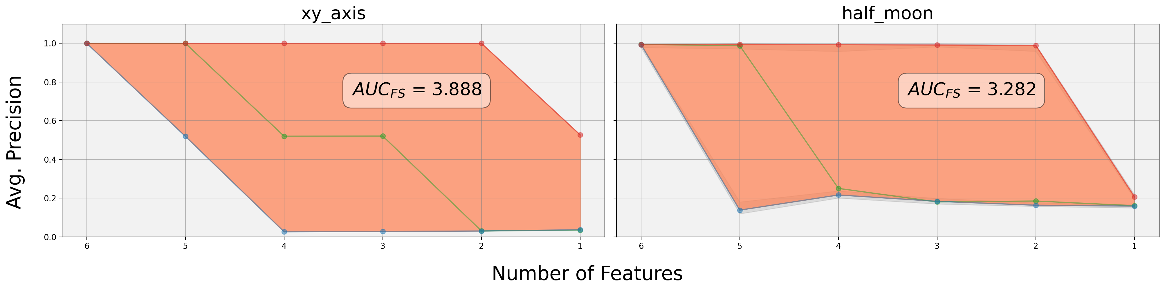
Specifically, for xy_axis (left figure in 6), the two anomaly clusters are independently caused by different features. Removing one of them from the input space (e.g., feature 1) results in a reduction of average precision; however, the model can still detect anomalies since the cluster aligned along feature 0 remains identifiable.

Conversely, for half_moon (right figure in 6), features 0 and 1 are jointly relevant. Excluding either feature from the feature space causes the average precision to drop to approximately zero, as anomalies cannot be detected without both features.

Figure 7: LFI scatter plot for synthetic datasets: xy_axis in blue and half_moon in orange

The Feature Selection plots may yield misleading interpretations: for xy_axis, the equal-sized clusters cause average precision to be halved when one key feature is removed, which would differ with imbalanced outlier groups. The LFI scatter plots in Figure 7 provide a more robust evaluation. These visualizations depict the LFI scores for features 0 and 1 across the two scenarios.

As expected, xy_axis (in blue) reveals two well-separated clusters: one group exhibits high LFI scores on feature 0 and low scores on feature 1, and vice versa. In contrast, half_moon (in orange) shows that the LFI scores are aligned along the bisector line of the subspace formed by the two important features, demonstrating their joint importance in anomaly detection.

4.10 Ablation Studies

In this section ablation studies are performed on some key EIF and ExIFFI hyperparameters to assess their influence on model performances. The considered hyperparameters are the number of isolation trees used to fit the ensemble and the contamination factor (i.e. the percentage of anomalies in the data). The latter has a crucial importance in industrial settings where labelled data are not available and thus the contamination factor has to be set without any objective grounding.

Ablation studies were conducted also on other hyperparameters (i.e. max_depth and max_samples) but the results demonstrate their minimal dependence with detection performances (i.e. average precision) and are thus not included in this study. For the interested reader, ablation studies on the $\eta$ hyperparameter are reported in [3].

In these experiments we observed the trend of some AD and interpretability metrics for different hyperparameters values. For this reason these were conducted on datasets containing ground truth knowledge on the anomalous data like TEP and CoffeeData.

For the sake of space only the results on the TEP dataset are reported but the ones obtained on CoffeeData are not much different.

4.10.1 Number of Trees

This experiment consists in tracking the variation of the average precision AD metric as the number of trees used to fit the underlying AD model increases. More trees expose the model to higher data variability, improving anomaly detection. Average precision is expected to increase with the ensemble size, at the cost of longer fitting and prediction times.

Figure 8: The average precision metric increases as the number of trees used to fit the AD model increases

Figure 8 shows improvement from 10 to 30 trees, with performance saturating at 93% average precision beyond 50 trees, suggesting 50 trees suffice for TEP. Computational time grows linearly with the number of estimators (not shown for space).

4.10.2 Contamination Prediction

In AD models the contamination factor is used to set a threshold on the anomaly scores in order to convert them into binary label to classify a point as anomalous or not. Consequently is crucial to correctly set this quantity, especially in industrial settings.

We vary the contamination level and measure ROC AUC of $\text{EIF}^{+}$, testing values both above and below the true contamination ($\approx 4\%$ for TEP), evaluating the effect of false negatives (underestimation) and false positives (overestimation).

Figure 9: Impact of contamination level on the ROC AUC score (top figure) and on the $AUC_{FS}$ metric. In both cases the best performances are obtained near the true dataset contamination value, indicated by the red vertical line. The x-axis is visualized in logarithmic scale.

The top plot of Figure 9 shows the impact of contamination level on ROC AUC performance, exhibiting a bell-shaped curve whose maximum occurs at approximately the true dataset contamination value. Notably the curve is almost symmetric, meaning that a significant overestimation produces a similar effect on the ROC AUC score as an underestimation.

4.10.3 Contamination Feature Selection

This ablation evaluates interpretability via the $AUC_{FS}$ metric (Section 4.2), again varying contamination since it affects GFI computation (Section 3), using the same values as in Section 4.10.2.

The bottom plot of Figure 9 shows a similar U-shaped curve, but $AUC_{FS}$ values are much lower for underestimated contamination, likely because too few anomalies are available for GFI computation. This supports the preference for overestimating contamination, as false positives are less harmful than false negatives.

5 Limitations and Future Work

Despite the results reported in 4.3, some limitations have to be considered for a full integration of ExIFFI into IIoT infrastructure.

The main limitation is the lack of flexibility: ExIFFI is tailored to EIF and $\text{EIF}^{+}$, unlike AcME-AD and KernelSHAP which are model-agnostic. This limitation creates a trade-off between flexibility and efficiency. Nonetheless, as showcased in Table 8, the specificity of ExIFFI results in fitting, inference and explanation times that are orders of magnitude smaller than those of AcME-AD and, especially, KernelSHAP. In the context of an industrial application, where execution times are critical, we believe this efficiency gain outweighs the lack of flexibility, making ExIFFI more practical than the tested alternatives.

Another limitation is the inability to detect clustered anomalies, as discussed in 3. This can be partially mitigated by the bootstrapping used during isolation forest training: if clusters are small, anomalies may be isolated in different trees, improving detectability. For large clusters, however, anomalies become ill-defined and this mitigation fails. Semi-supervised AD methods [40] have shown promising results in such cases and represent a direction for future work in industrial settings.

6 Conclusions

We demonstrate ExIFFI for industrial AD, providing interpretable model explanations through informative visualizations that integrate algorithmic outputs with domain expert knowledge.

ExIFFI was tested on four datasets coming from different industrial settings, equipped with high data dimensionality, unlabeled data points and non linear sensor interactions. The explanations provided by ExIFFI aligned with the ground truth on the anomalies’ root cause features. The effectiveness of the interpretations was proved against state-of-the-art interpretability methods through the Feature Selection proxy task, as shown in Sections 4.4.2,4.6.2.

ExIFFI outperforms competing interpretability methods in computational efficiency (Section 4.7), a key requirement in industrial settings. This stems from being model-specific to EIF, one of the most time-efficient AD models.

The computational efficiency and low memory footprint of ExIFFI make it suitable for deployment in a TinyML [7] IIoT framework, as showcased in 4.8, positioning it as a practical real-time AD and feature importance tool for Industry 5.0.

References

- [1] (2016) Outlier analysis. 2nd edition, Springer Publishing Company, Incorporated. External Links: ISBN 3319475770 Cited by: §4.3.
- [2] (2022) From artificial intelligence to explainable artificial intelligence in industry 4.0: a survey on what, how, and where. IEEE Trans. on Ind. Informatics 18 (8), pp. 5031–5042. Cited by: §1.
- [3] (2024) Enhancing interpretability and generalizability in extended isolation forests. Eng. App. of Artificial Intelligence 138, pp. 109409. External Links: ISSN 0952-1976, Document, Link Cited by: §1, §4.10, §4.4.2, §4.9.
- [4] (2022) Symbiotic relationship between machine learning and industry 4.0: a review. J. of Ind. Integration and Management 7 (03), pp. 401–433. Cited by: §1.
- [5] (2024) Unsupervised anomaly detection algorithms on real-world data: how many do we need?. J. of Machine Learning Research 25 (105), pp. 1–34. External Links: Link Cited by: §1, §3.
- [6] (2022) An explainable artificial intelligence approach for unsupervised fault detection and diagnosis in rotating machinery. Mechanical Systems and Signal Processing 163, pp. 108105. Cited by: §2.
- [7] (2024) A machine learning-oriented survey on tiny machine learning. IEEE Access 12 (), pp. 23406–23426. External Links: Document Cited by: §6.
- [8] (2019) A deep learning approach for anomaly detection with industrial time series data: a refrigerators manufacturing case study. Procedia Manufacturing 38, pp. 233–240. Cited by: §2.
- [9] (2019) Explainable machine learning in industry 4.0: evaluating feature importance in anomaly detection to enable root cause analysis. In 2019 IEEE Int. Conf. on systems, man and cybernetics (SMC), pp. 21–26. Cited by: §1.
- [10] (2020) Interpretable anomaly detection for knowledge discovery in semiconductor manufacturing. In 2020 Winter Simulation Conf. (WSC), pp. 1875–1885. Cited by: §2.
- [11] (2023) Interpretable anomaly detection with diffi: depth-based feature importance of isolation forest. Eng. App. of Artificial Intelligence 119, pp. 105730. Cited by: §2, §4.4.2.
- [12] (2026) Sensor fusion transformer for interpretable anomaly detection via multi-sensor time series data. Engineering Applications of Artificial Intelligence 164, pp. 113049. External Links: ISSN 0952-1976, Document, Link Cited by: §2.
- [13] (2026) GenAD-sm: optimized transformer-vae model for precision anomaly detection for smart manufacturing in industry 5.0. Journal of Intelligent Manufacturing. External Links: Document Cited by: §2.
- [14] (2022) FORMULA: a deep learning approach for rare alarms predictions in industrial equipment. IEEE Trans. on Automation Science and Eng. 19 (3), pp. 1491–1502. External Links: Document Cited by: §4.7.
- [15] (2023) A survey of ai-based anomaly detection in iot and sensor networks. Sensors 23. External Links: Link Cited by: §1.
- [16] (2019) Dynamic process fault detection and diagnosis based on a combined approach of hidden markov and bayesian network model. Chemical Eng. Science 201, pp. 82–96. Cited by: §4.4.1.
- [17] (2020) Interpretable anomaly detection for knowledge discovery in semiconductor manufacturing. In Proceedings of the 2020 Winter Simulation Conference, Cited by: §2.
- [18] (2024) Interpretable data-driven anomaly detection in industrial processes with exiffi. In 2024 IEEE 8th Forum on Research and Technologies for Society and Industry Innovation (RTSI), pp. 595–600. Cited by: §1, §3, §4.1, §4.2, §4.5.1.
- [19] (2022) A review paper on wireless sensor network techniques in internet of things (iot). Materials Today: Proceedings 51, pp. 161–165. Cited by: §1.
- [20] (2022) ADBench: anomaly detection benchmark. External Links: 2206.09426, Link Cited by: §2.
- [21] (2021) Extended isolation forest. IEEE Trans. on Knowledge and Data Engineering 33 (4), pp. 1479–1489. External Links: Document Cited by: §1, §3.
- [22] (2014) Industry 4.0. Business & Inf. systems Eng. 6, pp. 239–242. Cited by: §2.
- [23] (2008) Isolation forest. In 2008 Eight IEEE Int. Conf. on Data Mining, Vol. , pp. 413–422. External Links: Document Cited by: §1.
- [24] (2017) A unified approach to interpreting model predictions. Advances in neural information processing systems 30. Cited by: §2, §4.4.2.
- [25] (2020) Interpretable machine learning. Lulu. com. Cited by: §2.
- [26] (2017) Additional Tennessee Eastman Process Simulation Data for Anomaly Detection Evaluation. Harvard Dataverse. External Links: Document, Link Cited by: Table 1, §4.
- [27] (2018-10–15 Jul) Deep one-class classification. In Proceedings of the 35th International Conference on Machine Learning, J. Dy and A. Krause (Eds.), Proceedings of Machine Learning Research, Vol. 80, pp. 4393–4402. External Links: Link Cited by: §4.3.
- [28] (2025) Interpretable anomaly detection in encrypted traffic using shap with machine learning models. External Links: 2505.16261, Link Cited by: §2.
- [29] (2018) Industrial internet of things: challenges, opportunities, and directions. IEEE Tran. on Ind. Informatics 14 (11), pp. 4724–4734. Cited by: §1.
- [30] (2019) Robust anomaly detection for multivariate time series through stochastic recurrent neural network. In Proceedings of the 25th ACM SIGKDD International Conference on Knowledge Discovery & Data Mining, KDD ’19, New York, NY, USA, pp. 2828–2837. External Links: ISBN 9781450362016, Link, Document Cited by: §4.1.1, Table 1, §4.
- [31] (2025) Anomaly detection for antenna-based defect detection in additive manufacturing: an explainable, instructive learning framework. In Second Workshop on XAI4Science: From Understanding Model Behavior to Discovering New Scientific Knowledge, External Links: Link Cited by: §2.
- [32] (2024) Supervised and unsupervised soft sensors for capsule recognition in espresso coffee machines. In 2024 IEEE 8th Forum on Research and Tech. for Society and Industry Innovation (RTSI), pp. 311–316. Cited by: §4.1.2, §4.1.2, §4.1.2, §4.1.2, §4.3, §4.3.
- [33] (2022) Packaging industry anomaly detection (piade) dataset. Note: Dataset Cited by: Table 1, §4.
- [34] (2023) Industry 5.0 and its technologies: a systematic literature review upon the human place into iot-and cps-based industrial systems. Computers & Ind. Eng. 184, pp. 109426. Cited by: §2.
- [35] (2021) Interpretable machine learning: a brief survey from the predictive maintenance perspective. In 2021 26th IEEE Int. Conf. on Emerging Technologies and Factory Automation (ETFA), Vol. , pp. 01–08. External Links: Document Cited by: §2.
- [36] (2019) DBSCAN: optimal rates for density based clustering. External Links: 1706.03113, Link Cited by: §3.
- [37] (2026) Interpretable maximum margin deep anomaly detection. External Links: 2603.07073, Link Cited by: §2, §2.
- [38] (2024) Acme-ad: accelerated model explanations for anomaly detection. In World Conf. on Explainable AI, pp. 441–463. Cited by: §2, §4.4.2, §4.7.
- [39] (2024) Enabling efficient and flexible interpretability of data-driven anomaly detection in industrial processes with acme-ad. In 2024 10th Int. Conf. on Control, Decision and Inf. Tech. (CoDIT), Vol. , pp. 1375–1380. External Links: Document Cited by: §2.
- [40] (2024) Extended b-alif: improving anomaly detection with human feedback. In 2024 32nd Mediterranean Conference on Control and Automation (MED), Vol. , pp. 555–560. External Links: Document Cited by: §5.
- [41] (2022) From industry 4.0 towards industry 5.0: a review and analyfsis of paradigm shift for the people, organization and technology. Energies 15 (14), pp. 5221. Cited by: §2.
- [42] (2026) Graph neural network solutions for interpretable anomaly detection in it infrastructure monitoring time series. Journal of Business Analytics 0 (0), pp. 1–20. External Links: Document, Link, https://doi.org/10.1080/2573234X.2025.2607576 Cited by: §2.