On Minimal Depth in Neural Networks

Abstract

Understanding the relationship between the depth of a neural network and its representational capacity is a central problem in deep learning theory. In this work, we develop a geometric framework to analyze the expressivity of ReLU networks with the notion of depth complexity for convex polytopes. The depth of a polytope recursively quantifies the number of alternating convex hull and Minkowski sum operations required to construct it. This geometric perspective serves as a rigorous tool for deriving depth lower bounds and understanding the structural limits of deep neural architectures.

We establish lower and upper bounds on the depth of polytopes, as well as tight bounds for classical families. These results yield two main consequences. First, we provide a purely geometric proof of the expressivity bound by Arora et al. (2018), confirming that $\lceil\log_{2}(n+1)\rceil$ hidden layers suffice to represent any continuous piecewise linear (CPWL) function. Second, we prove that, unlike general ReLU networks, convex polytopes do not admit a universal depth bound. Specifically, the depth of cyclic polytopes in dimensions $n\geq 4$ grows unboundedly with the number of vertices. This result implies that Input Convex Neural Networks (ICNNs) cannot represent all convex CPWL functions with a fixed depth, revealing a sharp separation in expressivity between ICNNs and standard ReLU networks.

1 Introduction

A ReLU neural network of depth $m$, or with $m$ hidden layers, is a function $f:\mathbb{R}^{n}\rightarrow\mathbb{R}$ expressed as

$$f=T^{(m+1)}\circ\sigma_{m}\circ T^{(m)}\circ\sigma_{m-1}\circ\dots\circ T^{(2)}\circ\sigma_{1}\circ T^{(1)},$$

where $T^{(l)}:\mathbb{R}^{n_{l-1}}\rightarrow\mathbb{R}^{n_{l}}$ are $m+1$ affine transformations, $n_{0}=n$ and $n_{m+1}=1$. The activation function $\sigma_{l}$ corresponds to the vectorized ReLU function $\sigma_{l}(x_{1},\ldots,x_{n_{l}})=(\max\{x_{1},0\},\max\{x_{2},0\},\ldots,\max\{x_{n_{l}},0\})$.

ReLU neural networks are continuous piecewise linear (CPWL) functions [2, 10]. An important problem in learning theory is to characterize which CPWL functions can be represented by a ReLU network of a given depth. Such expressivity results are relevant for quantifying depth-dependent convergence rates for various function classes [8, 9, 10, 26] and enhancing our theoretical understanding of deep architectures [2, 23, 11, 18].

We denote the set of all CPWL functions from $\mathbb{R}^{n}\rightarrow\mathbb{R}$ as $\mathsf{CPWL}_{n}$, and the subset of these functions that can be represented by ReLU networks of depth $m$ as $\mathsf{ReLU}_{n}(m)$.

It has been shown that $\lceil\log_{2}(n+1)\rceil$ hidden layers are sufficient to represent any CPWL function.

Theorem 1 (Arora, Basu, Mianjy and Mukherjee [2], Theorem 2.1).

$$\mathsf{CPWL}_{n}=\mathsf{ReLU}_{n}(\lceil\log_{2}(n+1)\rceil).$$

The minimal depth required to represent any CWPL function remains an open question. Hertrich, Basu, Di Summa, and Skutella [16] proposed an approach that reduces the problem to analyzing a single function.

Proposition 1 (Hertrich, Basu, Di Summa and Skutella [16], Proposition 1.6).

$$\mathsf{CPWL}_{n}=\mathsf{ReLU}_{n}(m)\Longleftrightarrow\max\{x_{1},x_{2},\ldots,x_{n},0\}\in\mathsf{ReLU}_{n}(m).$$

Following Proposition 1, the goal is to find the minimum $m$ such that the function $\max\{x_{1},\ldots,x_{n},0\}\in\mathsf{ReLU}_{n}(m)$.

Hertrich, Basu, Di Summa, and Skutella [16] also conjectured that this depth is exactly $\lceil\log_{2}(n+1)\rceil$, which had been proven for dimensions $n\leq 3$ [10, 20]. Much of the progress toward resolving this problem has come from formulating Proposition 1 in the language of convex polytopes, i.e. the convex hull of finitely many points [14, 29]. Haase, Hertrich, and Loho [15] proved the conjecture for ReLU networks with integer weights. This result was later extended by Averkov, Hojny, and Merkert [3] to networks with decimal fractional weights. Furthermore, Grillo, Hertrich, and Loho [13] proved the conjecture for $n=4$ in networks compatible with specific polyhedral complexes. More recently, the conjecture was disproved by Bakaev, Brunck, Hertrich, Stade, and Yehudayoff [5] via polyhedral subdivisions of the simplex; they showed that $\lceil\log_{3}(n-1)\rceil+1$ hidden layers are sufficient to represent any CPWL function.

In this work, we introduce the depth complexity of polytopes, a geometric analogue of neural network depth, to analyze the expressivity of ReLU networks. Although this concept has been used implicitly in prior work [16, 15, 5], we provide a systematic study of it.

We denote the depth complexity of a polytope $P$ as $d(P)$ and define it recursively as follows. If $P$ consists of a single point, we define $d(P)=0$. If $P$ is not a single point, we define $d(P)=m$, where $m$ is the smallest positive integer such that

$$P=\sum_{i=1}^{q}\mathrm{conv}(P_{i1},P_{i2}),\quad\text{with }d(P_{ij})<m\quad\forall i,j.$$ (1)

Here, $\mathrm{conv}(P_{1},P_{2})=\mathrm{conv}(P_{1}\cup P_{2})$ and $P_{1}+P_{2}=\{a_{1}+a_{2}:a_{i}\in P_{i}\}$ are the convex hull and Minkowski sum operations respectively.

At its core, the depth complexity of a polytope quantifies the number of alternating steps of convex hulls and Minkowski sums required to construct it. This serves as a measure of how “complex” it is to represent a polytope using these two operations. Under this measure, the simplest polytope is a point and depth-1 polytopes correspond to zonotopes, which are Minkowski sums of segments.

Before connecting the depth of polytopes and ReLU networks, we introduce some terminology. A linear max function is a function of the form $f(x)=\max\{a_{1}\cdot x,\ldots,a_{p}\cdot x\}$ with $a_{i}\in\mathbb{R}^{n}$ for all $i$. Notably, linear max functions are convex and positively homogeneous, meaning they satisfy $f(\lambda x)=\lambda f(x)$ for $\lambda\geq 0$.

Let $\mathsf{LM}_{n}$ denote the collection of linear max functions from $\mathbb{R}^{n}\rightarrow\mathbb{R}$, and let $\mathcal{P}_{n}$ represent the set of convex polytopes in $\mathbb{R}^{n}$. These two sets constitute semirings with the max and sum operations, and convex hull and Minkowski sum operations, respectively.

For the function $f(x)=\max\{a_{1}\cdot x,\ldots,a_{p}\cdot x\}$, its Newton polytope is defined as

$$\mathcal{N}f:=\mathrm{conv}(a_{1},\ldots,a_{p}).$$

Similarly, for the polytope $P=\mathrm{conv}(a_{1},\ldots,a_{p})$, the associated support function is

$$\mathcal{F}P(x):=\max\{a_{1}\cdot x,\ldots,a_{p}\cdot x\}.$$

The mappings $\mathcal{N}$ and $\mathcal{F}$ are isomorphisms between the semirings ($\mathsf{LM}_{n}$, max, $+$) and ($\mathcal{P}_{n}$, conv, $+$) [19, 28].

The following result establishes a depth connection between ReLU networks and polytopes.

Theorem 2 (Hertrich, Basu, Di Summa and Skutella [16], Theorem 5.2).

Let $f\in\mathsf{CPWL}_{n}$ be a positively homogeneous function. Then, $f\in\mathsf{ReLU}_{n}(m)$ if and only if there exist $f_{i}\in\mathsf{LM}_{n},i=1,2,$ such that $f=f_{1}-f_{2}$ and $d(\mathcal{N}f_{i})\leq m$.

Combining Proposition 1 with Theorem 2 gives an equivalent geometric statement of Proposition 1.

Theorem 3.

$$\mathsf{CPWL}_{n}=\mathsf{ReLU}_{n}(m)$$

if and only if there exist polytopes $P_{i},i=1,2,$ such that

$$P_{1}=\mathcal{N}(\max\{x_{1},x_{2},\ldots,x_{n},0\})+P_{2}\quad\text{and}\quad d(P_{i})\leq m.$$

To fully leverage Theorem 3, it is relevant to establish foundational results on the depth complexity of polytopes. In addition, two natural questions arise: What is the minimum depth required to represent any polytope? And, what is the depth complexity of simplices like $\mathcal{N}(\max\{x_{1},x_{2},\ldots,x_{n},0\})$?

Depth Complexity Results

In Section 2, we derive depth complexity upper bounds based on Minkowski sums, affine transformations, convex hull representations, and combinatorial data such as the number of vertices, edges, and 2-faces. Combined with Theorem 2, these bounds yield depth estimates for ReLU network representations of linear max functions.

An affine transformation is a mapping $\varphi(x)=Ax+b$, where $A$ is a linear map and $b$ is a translation vector. A convex hull representation of a polytope $P$ in terms of other polytopes $P_{1},\ldots,P_{k}$ is a decomposition of the form $P=\mathrm{conv}(P_{1},P_{2},\ldots,P_{k})$.

If the polytopes $P_{i}$ are the vertices, edges or 2-faces of $P$, we can compute depth estimates based on their counts. For a polytope with $k$ vertices, we obtain the upper bound $\lceil\log_{2}k\rceil$, which is tight for certain families of polytopes.

In Section 3, we derive lower bounds on depth complexity using its graph and face structure. Let $G(P)$ denote the 1-skeleton of $P$, i.e. the graph whose vertices are those of $P$ and in which two vertices are adjacent when they span an edge of $P$.

We show that if $G(P)$ contains a complete subgraph on $k$ vertices, then $d(P)\geq\lceil\log_{2}k\rceil$. This follows from the fact that complete subgraphs are pervasive in expressions like (1): if $G(P)$ contains a complete subgraph, then at least a summand in the Minkowski sum will have one, which then propagates through the polytopes in the convex hull.

Moreover, for any face $F$ of $P$, we have $d(F)\leq d(P)$. Hence, $d(P)$ is at least the maximum depth complexity among its faces.

In Section 4, we determine the depth complexity of several families of polytopes, including pyramids, bipyramids, prisms, simplices, and cyclic polytopes. Using depth estimates based on vertex counts and complete subgraphs, it follows directly that polytopes with $k$ vertices whose graphs are complete, such as simplices and cyclic polytopes, have depth complexity $\lceil\log_{2}k\rceil$.

This result answers both motivating questions posed earlier. For simplices, the main application follows from Theorem 3, where we recover the same bound as in Theorem 1, thus providing an alternative geometric proof. In contrast, for dimension $n\geq 4$, cyclic polytopes form a family whose depth grows unbounded as the number of vertices increases. This shows that there is no universal upper depth bound to represent polytopes–unlike the case for ReLU networks in Theorem 1. Notably, the proofs of these results rely only on elementary polyhedral theory.

We conclude Section 4 by showing that cyclic polytopes not only exhibit unbounded depth, but in dimensions $n\geq 5$, their Minkowski sum with zonotopes yield, for any given depth $m$, families of polytopes with an increasing number of vertices, all of depth $m$.

Implications for Input Convex Neural Networks

Input Convex Neural Networks (ICNNs) [1] are ReLU networks constrained to use only monotone affine transformations and skip connections from the input layer. Here, a monotone affine transformation means an affine map $Ax+b$ where the matrix $A$ has nonnegative entries.

ICNNs are interesting because they can represent any convex CPWL function [4, 12] and have found many successful applications [17, 25, 6, 7].

Following [4], we can define under the ICNN model, a corresponding depth complexity $d_{0}(P)$ for a polytope $P$: $d_{0}(P)=0$ if $P$ is a single point, else $d_{0}(P)=m$ for $m$ the minimum value such that

$$P=\sum_{i=1}^{p}\mathrm{conv}(P_{i1},P_{i2}),\quad\text{with }d_{0}(P_{i1})<m\text{ and }d_{0}(P_{i2})=0\quad\forall i.$$

In [4] the authors showed that $d_{0}(\mathcal{N}(\max\{x_{1},\ldots,x_{n}\}))=n$, and that for $n=3$ there exists a family of polytopes with unbounded $d_{0}$-complexity. For ICNNs, $d_{0}(P)$ also constitutes the minimum ICNN depth required to represent $\mathcal{F}P$.

Since $d(P)\leq d_{0}(P)$, and cyclic polytopes with $k$ vertices satisfy $d(P)=\lceil\log_{2}k\rceil$ for $n\geq 4$, they also form an unbounded depth family for $d_{0}$. Thus, although ICNNs can represent every convex CPWL function, no fixed depth bound suffices in general. This contrasts with the universal depth bound for ReLU networks established in Theorem 1.

Acknowledgements. I am deeply grateful to Francisco Santos for Theorem 4, valuable discussions, and his hospitality at the University of Cantabria. I also thank Ansgar Freyer for discussions on the depth complexity of simplices.

2 Depth Upper Bounds

We begin by computing basic bounds for Minkowski sums, convex hulls and affine maps.

Proposition 2.

Let $P_{i},i=1,2,$ be polytopes with $d(P_{i})\leq m_{i}$ and $\varphi$ be an affine transformation. Then,

1. $d(P_{1}+P_{2})\leq\max\{m_{1},m_{2}\}$

2. $d(\mathrm{conv}(P_{1},P_{2}))\leq\max\{m_{1},m_{2}\}+1$

3. $d(\varphi(P_{1}))\leq d(P_{1})$

Proof.

These depth bounds follow immediately from the depth complexity definition. If $d(P_{i})\leq m_{i}$, it implies that we can express $P_{i}$ as

$$P_{i}=\sum_{j=1}^{q_{i}}\mathrm{conv}(Q_{j,i},R_{j,i}),\quad d(Q_{j,i}),d(R_{j,i})<m_{i}\quad\forall i,j.$$

Then,

$$P_{1}+P_{2}=\sum_{j=1}^{q_{1}}\mathrm{conv}(Q_{j,1},R_{j,1})+\sum_{j=1}^{q_{2}}\mathrm{conv}(Q_{j,2},R_{j,2}).$$

All $Q_{j,i}$ and $P_{j,i}$ have depth strictly less than $\max\{m_{1},m_{2}\}$, therefore $d(P_{1}+P_{2})\leq\max\{m_{1},m_{2}\}$.

Similarly, since $d(P_{i})\leq\max\{m_{1},m_{2}\}$, it follows by definition that

$$d(\mathrm{conv}(P_{1},P_{2}))\leq\max\{m_{1},m_{2}\}+1.$$

Let $\varphi(x)=Ax+b$ be an affine map, if $d(P_{1})=0$, it is trivial that $d(\varphi(P_{1}))=0$. For the purpose of induction, assume the statement is true up to $m-1$. If $d(P_{1})=m$, then

$$\varphi(P_{1})=\varphi\Big(\sum_{j=1}^{q_{1}}\mathrm{conv}(Q_{j,1},R_{j,1})\Big)=\sum_{j=1}^{q_{1}}\mathrm{conv}(AQ_{j,1},AR_{j,1})+b,$$

and by induction hypothesis $d(AQ_{j,1}),d(AR_{j,1})<m$, implying $d(\varphi(P_{1}))\leq d(P_{1})$. ∎

If an affine transformation $\varphi$ is invertible, note that $d(\varphi(P))=d(P)$. This also implies that $d(P_{1}+P_{2})=d(P_{1})$ for $d(P_{2})=0$, which is simply a translation.

When $P=\mathrm{conv}(P_{1},\ldots,P_{k})$, iterating Proposition 2(b) can yield an upper bound for $d(P)$. If a common depth bound is known for each $P_{i}$, Proposition 3 gives a simple estimate for $d(P)$. Otherwise, combining the polytopes with smallest depth first yields the best upper bound achievable by iterating Proposition 2(b); see Appendix A.

Proposition 3.

Let $P$ be a polytope expressed as $P=\mathrm{conv}(P_{1},\ldots,P_{k})$ where $d(P_{i})\leq m$ for all $i$, then $d(P)\leq\lceil\log_{2}k\rceil+m$.

Proof.

We proceed by induction on $k$. The base case $k=1,2$ are immediate. For the induction step, assume the statement holds for all values strictly less than $k$.

Let $p$ be the largest power of $2$ such that $p<k$, and decompose $P$ as

$$P=\mathrm{conv}(\mathrm{conv}(P_{1},\ldots,P_{p}),\;\mathrm{conv}(P_{p+1},\ldots,P_{k})).$$

Since $p<k\leq 2p$, we have $k-p\leq p$, so the induction hypothesis gives

$$d(\mathrm{conv}(P_{1},\ldots,P_{p})) \leq\log_{2}p+m,$$

$$d(\mathrm{conv}(P_{p+1},\ldots,P_{k})) \leq\lceil\log_{2}(k-p)\rceil+m\leq\log_{2}p+m.$$

Applying Proposition 2(b) yields $d(P)\leq\log_{2}p+1+m=\lceil\log_{2}k\rceil+m$. ∎

We will use Proposition 3 to obtain estimates when the numbers of low-dimensional faces are known. For this, we need the following concepts: $\rho(P)$ and $\rho_{2}(P)$ are the minimum number of edges and 2-faces, respectively, needed to cover all vertices of the polytope $P$; $\nu(P)$ is the size of a maximum matching of the graph $G(P)$, i.e. the largest set of edges in $G(P)$ with no common vertices; $P_{x}$ is the vertex figure of $P$ at a vertex $x$, i.e. the intersection of $P$ with a hyperplane that separates $x$ from the other vertices of $P$.

Proposition 4.

Let $f_{0},f_{1},f_{2}$ be the number of vertices, edges and 2-faces respectively of a polytope $P$. Then, we have the following depth bounds depending of each $f_{i}$ individually:

1. $\text{For }f_{0}:\quad d(P)\leq\lceil\log_{2}f_{0}\rceil$

2. $\text{For }f_{1}:\quad d(P)\leq\Big\lceil\log_{2}\Big(\Big\lfloor\frac{2f_{1}}{n}-\min\Big(n,\Big\lfloor\frac{1+\sqrt{1+8f_{1}}}{4}\Big\rfloor\Big)\Big\rfloor\Big)\Big\rceil+1$

3. $\text{For }f_{2}:\quad d(P)\leq\Big\lceil\log_{2}\Big(f_{2}-\binom{n}{2}+1\Big)\Big\rceil+2$

Proof.

Any polytope $P$ can be expressed as $P=\mathrm{conv}(P_{1},\ldots,P_{f_{j}})$, where $P_{i}$ are $j$-dimensional faces of $P$.

(a) If $P_{i}$ are the vertices, then $d(P_{i})=0$, and by Proposition 3 we obtain

$$d(P)\leq\lceil\log_{2}f_{0}\rceil.$$

(b) If $P_{i}$ are the edges of $P$, then $d(P_{i})=1$. We do not need all $f_{1}$ edges as $P$ can be written as

$$P=\mathrm{conv}(P_{i_{1}},\ldots,P_{i_{\rho(P)}}),$$

where $\rho(P)$ is the size of a minimum edge cover $P_{i_{1}},\ldots,P_{i_{\rho(P)}}$.

To estimate $\rho(P)$, we use standard relations between $\rho(P)$, $\nu(P)$, $f_{0}$, and $f_{1}$ (see [24, Chapter 3.1]):

$$\rho(P)+\nu(P)=f_{0},\qquad\nu(P)\geq\min\big(n,\lfloor f_{0}/2\rfloor\big).$$

Furthermore, the degree sum formula and the complete graph vertices bound yield

$$nf_{0}\leq 2f_{1}\leq f_{0}(f_{0}-1).$$

Combining these inequalities gives

$$\rho(P)\leq\Big\lfloor\frac{2f_{1}}{n}-\min\Big(n,\Big\lfloor\tfrac{1+\sqrt{1+8f_{1}}}{4}\Big\rfloor\Big)\Big\rfloor,$$

from which the stated bound on $d(P)$ in terms of $f_{1}$ follows.

(c) Consider the case of $2$-faces. In Section 4 we show that the depth complexity of polygons is at most $2$. Hence, similarly as (b), it suffices to bound $\rho_{2}(P)$, the minimum number of $2$-faces covering all vertices of $P$, and apply Proposition 3.

Let $P_{x}$ be the vertex figure of $P$ at a vertex $x$. Since $\dim P_{x}=n-1$, the degree sum formula implies that $P_{x}$ has at least $\binom{n}{2}$ edges. These correspond bijectively to the $2$-faces of $P$ incident to $x$. Thus, even after removing any $\binom{n}{2}-1$ $2$-faces, every vertex of $P$ is still contained in at least one $2$-face. Hence $\rho_{2}(P)\leq f_{2}-\binom{n}{2}+1$, which yields

$$d(P)\leq\Big\lceil\log_{2}\big(f_{2}-\binom{n}{2}+1\big)\Big\rceil+2.\qed$$

3 Depth Lower Bounds

In this section, we study depth lower bounds for polytopes, obtained from their graphs and from the depth complexity of their faces.

Proposition 5.

Let $P$ be a polytope. Then for any nonempty face $F$ of $P$, we have $d(P)\geq d(F)$.

Proof.

If $d(P)=0$, there is nothing to prove. If $d(P)=1$, then $P$ is a zonotope, and any face $F$ is also a zonotope, hence $d(F)\leq 1$.

Now suppose, for induction, that the statement holds for all polytopes of depth at most $m-1$, and assume $d(P)=m$. By definition, we can write

$$P=\sum_{i=1}^{q}\mathrm{conv}(P_{i1},P_{i2}),\quad d(P_{ij})<m\quad\forall i,j.$$

Let $F$ be a face of $P$. Then $F=\sum_{i=1}^{q}F_{i}$, where each $F_{i}$ is a face of $\mathrm{conv}(P_{i1},P_{i2})$. This implies that $F_{i}$ can be written as $F_{i}=\mathrm{conv}(F_{i1},F_{i2})$, where $F_{ij}$ is a (possibly empty) face of $P_{ij}$.

By the induction hypothesis, whenever $F_{ij}\neq\emptyset$, we have $d(F_{ij})<m$. If both $F_{i1}$ and $F_{i2}$ are nonempty, then by Proposition 2(b) we have $d(F_{i})\leq m$. If exactly one of $F_{i1},F_{i2}$ is nonempty, then $F_{i}$ is equal to that nonempty face, and hence $d(F_{i})\leq m$.

Therefore, in all cases each $F_{i}$ satisfies $d(F_{i})\leq m$. Finally, since $F=\sum_{i=1}^{q}F_{i}$, Proposition 2(a) implies $d(F)\leq m=d(P)$. ∎

To obtain a lower bound from complete subgraphs contained in $G(P)$, we first state the following lemma.

Lemma 1.

If the graph of a polytope $G(P)$ contains a complete subgraph with $k\geq 3$ vertices, and $P$ can be decomposed as $P=\sum_{i=1}^{q}P_{i}$, then at least one of $G(P_{i})$ also contains a complete subgraph with $k$ vertices.

Proof.

Any edge $e=[x_{1},x_{2}]$ of $P$ can be written as $e=\sum_{i=1}^{q}e_{i}$, where each $e_{i}$ is either a vertex or an edge of $P_{i}$. If $e_{i}$ is a vertex, we regard it as a degenerate edge of length zero, so we can say that each edge of $P$ decomposes as a sum of edges of the $P_{i}$.

Now let $u,v,w$ be three vertices in the complete subgraph of $G(P)$ (so $[u,v],[u,w],[v,w]$ are edges of $P$). Write

$$[u,v]=\sum_{i=1}^{q}[u_{i},v_{i}],\quad[u,w]=\sum_{i=1}^{q}[u_{i},w_{i}],\quad[v,w]=\sum_{i=1}^{q}[v_{i},w_{i}],$$

where $u=\sum_{i}u_{i}$, $v=\sum_{i}v_{i}$, $w=\sum_{i}w_{i}$ with $u_{i},v_{i},w_{i}$ vertices of $P_{i}$.

The edges $[u_{i},v_{i}],[u_{i},w_{i}],[v_{i},w_{i}]$ are parallel to $[u,v],[u,w],[v,w]$ respectively, since otherwise their Minkowski sum would yield a polytope of dimension at least two, contradicting the fact that the corresponding sum is an edge. This implies that each triangle $[u_{i},v_{i},w_{i}]$ is homothetic to the triangle $[u,v,w]$, and therefore all edge length ratios are preserved

$$\frac{|u_{i}-v_{i}|}{|u-v|}=\frac{|u_{i}-w_{i}|}{|u-w|}=\frac{|v_{i}-w_{i}|}{|v-w|}.$$

Note that some triangles $[u_{i},v_{i},w_{i}]$ may be degenerate (if two or all three vertices coincide). In this case, the triangle is still homothetic to $[u,v,w]$ with homothety factor $0$, so the ratio identities above remain valid.

As the triangle $[u,v,w]$ is not degenerate, at least one index $j$ has these ratios nonzero, so $u_{j},v_{j},w_{j}$ are distinct vertices forming a triangle in $G(P_{j})$.

For any other vertex $z$ in the clique of $G(P)$, applying the same argument to the triangles $[u,v,z]$ and $[u,w,z]$ shows that the same index $j$ yields non-degenerate homothetic triangles $[u_{j},v_{j},z_{j}]$ and $[u_{j},w_{j},z_{j}]$, with $z_{j}$ distinct from $u_{j},v_{j},w_{j}$ and adjacent to them. Repeating this for every vertex in the clique, we conclude that $G(P_{j})$ contains a complete subgraph with $k$ vertices. ∎

Theorem 4.

If the graph of a polytope $G(P)$ contains a complete subgraph with $k\geq 3$ vertices, then $d(P)\geq\lceil\log_{2}k\rceil$.

Proof.

Suppose a subgraph of $G(P)$ is complete and contains $k=3$ or $k=4$ vertices. If we assume $d(P)=1$, then $P=\sum_{i=1}^{k}P_{i}$, where each $P_{i}$ is a segment. This contradicts Lemma 1, which implies that at least one $P_{i}$ must include $k$ vertices. Therefore, we conclude $d(P)\geq 2$.

For the sake of induction, let’s assume that the result holds for all cases up to $k-1$. Now, consider that $G(P)$ includes a complete subgraph consisting of $k$ vertices. By definition, we can express $P$ as

$$P=\sum_{i=1}^{q}\mathrm{conv}(P_{i},Q_{i}),\quad\textrm{where }d(P_{i}),d(Q_{i})<d(P).$$

According to Lemma 1, there exists an index $i$ for which $G(\mathrm{conv}(P_{i},Q_{i}))$ also contains a complete subgraph $K$ with $k$ vertices. Without loss of generality, we can assume that $P_{i}$ contains at least $\lceil\frac{k}{2}\rceil$ vertices of $K$.

If two vertices $x,y$ of $\mathrm{conv}(P_{i},Q_{i})$ span an edge, then they also span an edge in $P_{i}$ if $x,y\in P_{i}$. Hence $G(P_{i})$ contains not only at least $\lceil\frac{k}{2}\rceil$ vertices of $K$ but also the complete subgraph induced by them. By the induction hypothesis we obtain

$$d(P)-1\geq d(P_{i})\geq\Big\lceil\log_{2}\Big\lceil\frac{k}{2}\Big\rceil\Big\rceil=\big\lceil\log_{2}k\big\rceil-1,$$

from which it follows $d(P)\geq\lceil\log_{2}k\rceil$. ∎

4 Depth of Polytopes

Before computing the depth complexity of some polytope families, we first introduce a simple tool for indecomposable polytopes.

Two polytopes, $P$ and $Q$, are said to be positively homothetic, if $P=\lambda Q+w$ for some $\lambda>0$ and $w\in\mathbb{R}^{n}$. A polytope $P$ is said to be indecomposable if any decomposition $P=\sum_{i=1}^{k}P_{i}$ is only possible when $P_{i}$ is positively homothetic to $P$ for all $i=1,\ldots,k$.

Lemma 2.

If $P$ is an indecomposable polytope, then there exist polytopes $P_{1},P_{2}$ such that $P=\mathrm{conv}(P_{1},P_{2})$ and $d(P)=\max\{d(P_{1}),d(P_{2})\}+1$.

Proof.

By definition, if $d(P)=m$, then $P$ can be written as

$$P=\sum_{i=1}^{q}\mathrm{conv}(P_{i1},P_{i2}),\quad d(P_{ij})<m\quad\forall i,j,$$

where $m$ is the smallest integer for which such a representation exists. Hence there must exist an index $i$ such that $\max\{d(P_{i1}),d(P_{i2})\}+1=d(P)$.

Since $P$ is indecomposable, there are $\lambda_{i}>0$ and $w_{i}\in\mathbb{R}^{n}$ where $P$ satisfies

$$P=\lambda_{i}\mathrm{conv}(P_{i1},P_{i2})+w_{i}=\mathrm{conv}(\lambda_{i}P_{i1}+w_{i},\lambda_{i}P_{i2}+w_{i}).$$

Each $\lambda_{i}P_{ij}+w_{i}$ is an affine image of $P_{ij}$ under an invertible map. By Proposition 2(c), affine equivalence preserves depth, so

$$d(P)=\max\{d(P_{i1}),d(P_{i2})\}+1=\max\{d(\lambda_{i}P_{i1}+w_{i}),d(\lambda_{i}P_{i2}+w_{i})\}+1.\qed$$

We begin by computing the depth complexity of polygons, whose value is at most 2.

Polygons. $d(P)=1$ if $P$ is a zonotope, otherwise $d(P)=2$.

Proof.

If $P$ is a zonotope, then $d(P)=1$. If $P$ is a triangle, then $d(P)=2$ by Proposition 4(a), since a triangle is not a zonotope.

Now suppose $P$ is neither a zonotope nor a triangle. Then, $P$ can be decomposed as $P=\sum_{i=1}^{k}P_{i},$ where each $P_{i}$ is either a zonotope or a triangle [14, Chapter 15.1]. By Proposition 2(a), we obtain $d(P)=2$. ∎

A pyramid is a polytope of the form $P=\mathrm{conv}(Q,x)$, where $Q$ is the basis and $x\in\mathbb{R}^{n}$ such that $x\not\in\text{aff }Q$, the affine hull of $Q$.

Pyramids. $d(Q)\leq d(P)\leq d(Q)+1$, where $Q$ is a basis of $P$.

Proof.

From Proposition 2(b) we obtain $d(P)\leq d(Q)+1$. Since $Q$ is a face of $P$, Proposition 5 gives $d(Q)\leq d(P)$. ∎

A bipyramid is a polytope of the form $P=\mathrm{conv}(Q,x_{1},x_{2})$, where $Q$ (with $\dim Q\geq 1$) is the base, and $x_{1},x_{2}\notin\text{aff }Q$ are the apices, such that the segment $[x_{1},x_{2}]$ intersects the relative interior of $Q$.

Bipyramids. $d(Q)\leq d(P)\leq d(Q)+1$, where $Q$ is the basis of $P$.

Proof.

The upper bound $d(P)\leq d(Q)+1$ follows from Proposition 2(b). For the lower bound, let $H$ be a hyperplane containing aff $Q$ but not $x_{1},x_{2}$. Projecting $P$ onto $H$ along the line through the apices gives $Q$, hence by Proposition 2(c) we have $d(Q)\leq d(P)$. ∎

A prism is a polytope of the form $P=\mathrm{conv}(Q,x+Q)$, where $Q$ is called the base of $P$ and the translation $x+Q\notin\text{aff }Q$.

Prisms. $d(P)=d(Q)$, where $Q$ is the base of $P$.

Proof.

A prism with base $Q$ can be written as $P=Q+[\mathbf{0},x]$, where $[\mathbf{0},x]$ is a line segment from the origin. By Proposition 2(a), $d(P)\leq d(Q)$. Since $Q$ is a face of $P$, Proposition 5 gives $d(Q)\leq d(P)$. Thus $d(P)=d(Q)$. ∎

A 2-neighborly polytope $P$ is a polytope where the segment between any two vertices is an edge of $P$.

2-neighborly polytopes. $d(P)=\lceil\log_{2}k\rceil$, where $k$ is the number of vertices of $P$.

Proof.

Since $G(P)$ is complete, this follows from Proposition 4(a) and Theorem 4. ∎

As simplices are 2-neighborly we obtain directly their depth complexity.

Simplices. $d(P)=\lceil\log_{2}(n+1)\rceil$.

A nestohedron $P$ is a polytope of the form $P=\sum_{S\in\mathcal{S}}S$, where $\mathcal{S}$ is a collection of simplices. Examples include associahedra, permutohedra, cyclohedra, among others [21, 22].

Nestohedra. $d(P)\leq\lceil\log_{2}(\max_{S\in\mathcal{S}}\text{dim }S+1)\rceil\leq\lceil\log_{2}(n+1)\rceil$.

Proof.

This follows from the depth complexity of simplices together with Proposition 2(a). ∎

A cyclic polytope $C_{n}(k),k>n,$ is a polytope of the form

$$C_{n}(k)=\mathrm{conv}(\gamma(t_{1}),\ldots,\gamma(t_{k})),$$

where $t_{1}<\ldots<t_{k}$ are real numbers and $\gamma(t)=(t,t^{2},\ldots,t^{n})$. For $n\geq 4$, cyclic polytopes are 2-neighborly, therefore we obtain directly their depth complexity.

Cyclic polytopes. $d(C_{n}(k))=\lceil\log_{2}k\rceil$ for $n\geq 4$.

For $n=2$, polygons have bounded depth $d(P)\leq 2$. This contrasts with $n\geq 4$, where cyclic polytopes exhibit unbounded depth complexity as the number of vertices increases. The case $n=3$ remains open.

However, triangular bipyramids–bipyramids with a triangular basis–provide examples of 3-depth polyhedra. This shows that depth complexity in dimension $n=3$ behaves differently from the case $n=2$.

Triangular bipyramids in $R^{3}$. $d(P)=3$.

Proof.

A bipyramid with a 2-depth basis satisfies $2\leq d(P)\leq 3$. Assume, for contradiction, that $d(P)=2$. As $P$ is indecomposable [14, Chapter 15.1], Lemma 2 implies that there exist $P_{1},P_{2}$ such that $P=\mathrm{conv}(P_{1},P_{2})$ and $\max\{d(P_{1}),d(P_{2})\}+1=2$. Without loss of generality, suppose $P_{1}$ is a zonotope containing at least three vertices of $P$.

There are three cases: $P_{1}$ contains two base vertices and an apex; or the three base vertices; or one base vertex and the two apices. In each case $P_{1}$ is not centrally symmetric, contradicting that it is a zonotope. Hence $d(P)\neq 2$ and so $d(P)=3$. ∎

We conclude with a construction of polytopes with increasing number of vertices and fixed depth.

Theorem 5.

For any $n\geq 5$ and $m\in\mathbb{N}$, there exists a family of $n$-polytopes with unbounded number of vertices and depth $m$.

Proof.

Let $g_{i}=[\mathbf{0},b_{i}],i=1,\ldots,p$, represent line segments from the origin with $b_{1},\ldots,b_{p}$ denoting $p\geq n$ points in general position. The zonotope $Z_{p}=\sum_{i=1}^{p}g_{i}$ has depth 1 and $v_{p}=2\sum_{i=0}^{n-1}\binom{p-1}{i}$ vertices [27], which grows with $p$.

For any $m\geq 2$, let $H$ be a supporting hyperplane of a vertex $x$ of $Z_{p}$, and take a polytope $P\subset H$ with $\dim P<n$ and $d(P)=m$ (e.g. a simplex or cyclic polytope).

Then $P+Z_{p}$ satisfies $d(P+Z_{p})\leq m$ by Proposition 2(a). On the other hand, the face of $P+Z_{p}$ in the direction of $x$ is a translate of $P$, hence by Proposition 5, $m=d(P)\leq d(P+Z_{p})$. Thus $P+Z_{p}$ forms a $m$-depth family whose number of vertices increases with $p$. ∎

Similar constructions exist for $n\leq 4$ and $m\leq 3$, but a full generalization of Theorem 5 for $n=3,4$ and arbitrary $m$ would require a better understanding of depth complexity in dimension $3$.

Appendix A Extension to Proposition 3

To extend Proposition 3, we focus on convex hull representations of the form $P=\mathrm{conv}(P_{1},\ldots,P_{k})$, where $d(P_{i})\leq m_{i}$. To bound $d(P)$, we iteratively apply the convex hull estimate from Proposition 2(b) until all $k$ polytopes are covered.

For example, when $k=4$, we could proceed as follows:

$$d(P) =d(\mathrm{conv}(P_{1},P_{2},P_{3},P_{4}))$$

$$=d(\mathrm{conv}(\mathrm{conv}(P_{1},P_{2}),\mathrm{conv}(P_{3},P_{4})))$$

$$\leq\max\{\max\{m_{1},m_{2}\}+1,\max\{m_{3},m_{4}\}+1\}+1.$$

By repeatedly applying this convex hull estimate, we always obtain an upper bound for $d(P)$. Nevertheless, our goal is to determine the optimal way of carrying out this iteration. To formalize this, consider the set of natural numbers $(\mathbb{N},\ast)$, where the binary operation $\ast$ is defined by $a\ast b=\max\{a,b\}+1$. The operation $\ast$ is commutative but not associative, so the result of $m_{1}\ast m_{2}\ldots\ast m_{k}$ depends on the chosen order and parenthesization. Therefore, we want to find the arrangement that minimizes this value.

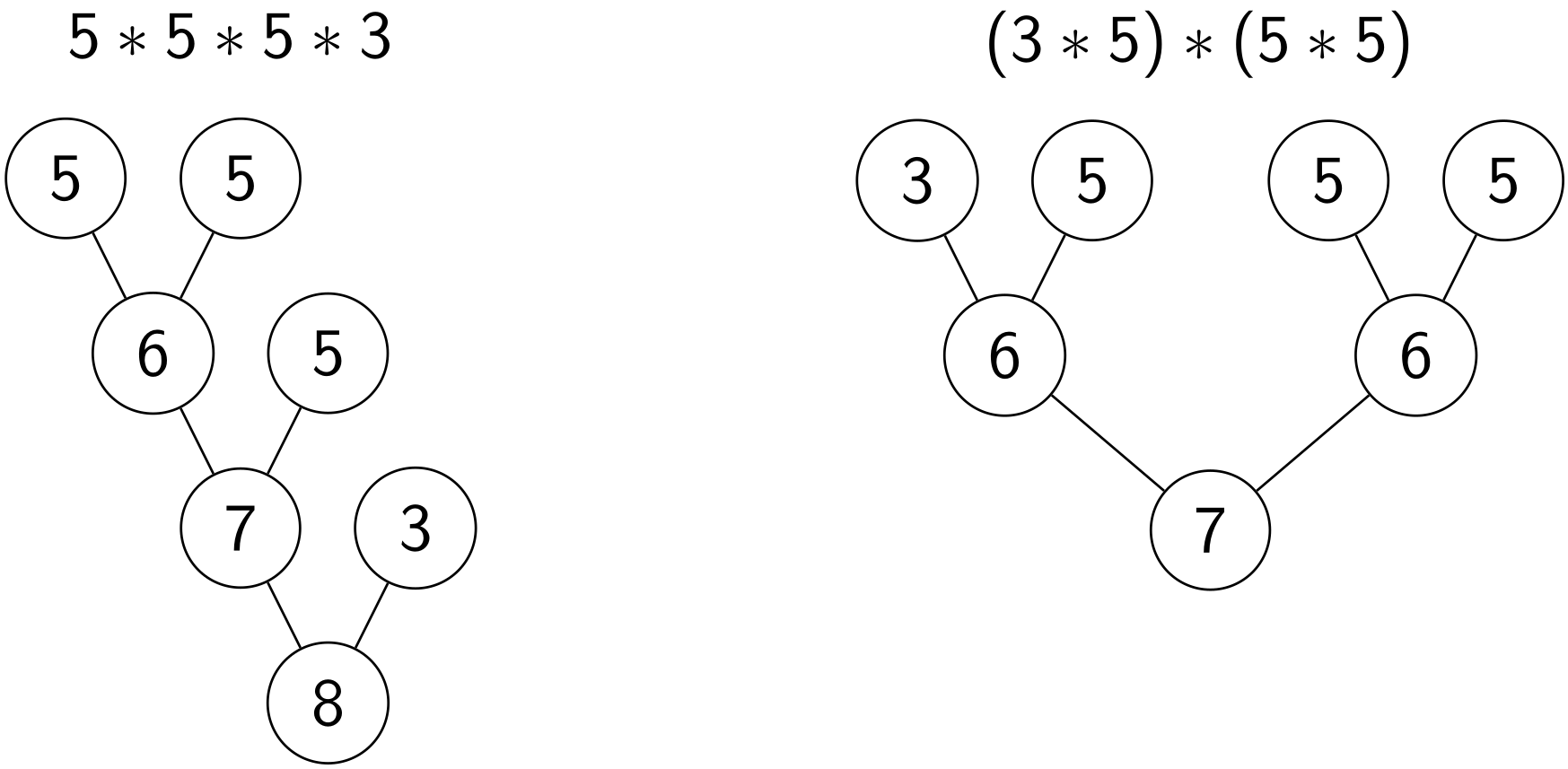
Given a choice of order and parenthesization, we can represent the expression as a full binary tree induced by $\ast$. The leaves of the tree correspond to the operands $m_{i}$, while each internal node stores the result of applying $\ast$ to its two children. The value of the root node is then the result of the entire expression. In Fig. 1, we illustrate two examples.

Figure 1: Two different order and parenthesization for $m_{1}\ast m_{2}\ast m_{3}\ast m_{4}$, with $m_{1}=m_{2}=m_{3}=5$ and $m_{4}=3$.

The main purpose of representing the $\ast$ operation with trees is to provide a tool for proving optimality. We call a tree induced by $\ast$ a $\ast$-tree, and we say that it is optimal for $m_{1},\ldots,m_{k}$ if, among all possible $\ast$-trees with leaves $m_{i}$, the root node’s value is minimal.

Directly from the definition of $\ast$, the root value of a $\ast$-tree equals $\max_{i}(m_{i}+p_{i})$, where $p_{i}$ is the depth of leaf $m_{i}$ (its distance to the root), since the $+1$ accumulates per level of depth and the $\max$ propagates the largest contribution to the root.

From this observation we can derive a simple strategy to obtain an optimal $\ast$-tree: at each step, apply $\ast$ to the two smallest available values. More precisely, suppose that at a given step the two smallest elements are $m_{i},m_{j}$. We compute $m_{i}\ast m_{j}$, replace them by this new value,

$$m_{i}\ast m_{j},m_{1},\ldots,m_{i-1},m_{i+1},\ldots,m_{j-1},m_{j+1},\ldots,m_{k},$$

and repeat the process with the updated list.

We call this procedure greedy selection, and iterating it until a single value remains yields a $\ast$-tree, which we refer as a greedy $\ast$-tree. The example on the right of Fig. 1 illustrates such a tree.

We show that every greedy $\ast$-tree is optimal. Note, however, that not every optimal $\ast$-tree is greedy.

Lemma 3.

A greedy $\ast$-tree is optimal.

Proof.

For the values $m_{1},\ldots,m_{k}$, we proceed by induction on $k$. The base cases $k=1,2$ are trivial. Assume the claim holds for $k-1$ operands.

Consider an optimal $\ast$-tree $T_{opt}$ for $m_{1}\leq m_{2}\leq\ldots\leq m_{k}$, with depth $p_{i}$ for the node containing the value $m_{i}$. Let $u$ and $v$ be two leaves at the maximum depth $D$ in $T_{opt}$. As leaves at the maximum depth in a full binary tree, $u$ and $v$ must be siblings.

If the values assigned to $u$ and $v$ are not $m_{1}$ and $m_{2}$, we can swap $m_{1}$ with the value at $u$ and $m_{2}$ with the value at $v$. Since $m_{1}$ and $m_{2}$ are the smallest values, and $u,v$ have the maximal depth $D$, moving $m_{1}$ and $m_{2}$ to these positions, and moving the original $u$ and $v$’s values to strictly shallower or equal depths, cannot increase the root’s value $\max_{i}(m_{i}+p_{i})$. Thus, there exists an optimal $\ast$-tree $T^{\prime}_{opt}$ where $m_{1}$ and $m_{2}$ are siblings.

In $T^{\prime}_{opt}$, assume the parent of $m_{1}$ and $m_{2}$ has value $m^{\prime}=\max(m_{1},m_{2})+1$. The rest of the tree forms an optimal $\ast$-tree for the reduced set of $k-1$ leaves $\{m^{\prime},m_{3},\ldots,m_{k}\}$. By the induction hypothesis, the greedy strategy finds an optimal $\ast$-tree for this reduced set, and expanding $m^{\prime}$ with the original values $m_{1},m_{2}$, yields a greedy $\ast$-tree optimal for the $k$ values. ∎

If $P$ is a polytope expressed as $P=\mathrm{conv}(P_{1},\ldots,P_{k})$, then Lemma 3 implies that a greedy selection for the computation of $d(P_{1})\ast d(P_{2})\ast\ldots\ast d(P_{k})$ yields the smallest possible value with these operands. Therefore, this minimum value gives the best upper bound for $d(P)$ achievable by iterating the convex hull estimate in Proposition 2(b) over the polytopes $P_{i}$.

References

- [1] Brandon Amos, Lei Xu, and J Zico Kolter. Input convex neural networks. In International conference on machine learning, pages 146–155. PMLR, 2017.
- [2] Raman Arora, Amitabh Basu, Poorya Mianjy, and Anirbit Mukherjee. Understanding deep neural networks with rectified linear units. In International Conference on Learning Representations, 2018.
- [3] Gennadiy Averkov, Christopher Hojny, and Maximilian Merkert. On the expressiveness of rational relu neural networks with bounded depth. In The Thirteenth International Conference on Learning Representations, 2025.
- [4] Egor Bakaev, Florestan Brunck, Christoph Hertrich, Daniel Reichman, and Amir Yehudayoff. On the depth of monotone relu neural networks and icnns. arXiv preprint arXiv:2505.06169, 2025.
- [5] Egor Bakaev, Florestan Brunck, Christoph Hertrich, Jack Stade, and Amir Yehudayoff. Better neural network expressivity: subdividing the simplex. arXiv preprint arXiv:2505.14338, 2025.
- [6] Felix Bünning, Adrian Schalbetter, Ahmed Aboudonia, Mathias Hudoba de Badyn, Philipp Heer, and John Lygeros. Input convex neural networks for building mpc. In Learning for dynamics and control, pages 251–262. PMLR, 2021.
- [7] Yize Chen, Yuanyuan Shi, and Baosen Zhang. Optimal control via neural networks: A convex approach. In International Conference on Learning Representations, 2019.
- [8] Ingrid Daubechies, Ronald DeVore, Nadav Dym, Shira Faigenbaum-Golovin, Shahar Z Kovalsky, Kung-Chin Lin, Josiah Park, Guergana Petrova, and Barak Sober. Neural network approximation of refinable functions. IEEE Transactions on Information Theory, 69(1):482–495, 2022.
- [9] Ingrid Daubechies, Ronald DeVore, Simon Foucart, Boris Hanin, and Guergana Petrova. Nonlinear approximation and (deep) relu networks. Constructive Approximation, 55(1):127–172, 2022.
- [10] Ronald DeVore, Boris Hanin, and Guergana Petrova. Neural network approximation. Acta Numerica, 30:327–444, 2021.
- [11] Ronen Eldan and Ohad Shamir. The power of depth for feedforward neural networks. In 29th Annual Conference on Learning Theory, volume 49, pages 907–940. PMLR, 2016.
- [12] Anne Gagneux, Mathurin Massias, Emmanuel Soubies, and Rémi Gribonval. Convexity in relu neural networks: beyond icnns? Journal of Mathematical Imaging and Vision, 67(4):40, 2025.
- [13] Moritz Grillo, Christoph Hertrich, and Georg Loho. Depth-bounds for neural networks via the braid arrangement. arXiv preprint arXiv:2502.09324, 2025.
- [14] Branko Grünbaum. Convex Polytopes. Springer, 2003.
- [15] Christian Alexander Haase, Christoph Hertrich, and Georg Loho. Lower bounds on the depth of integral relu neural networks via lattice polytopes. In International Conference on Learning Representations, 2023.
- [16] Christoph Hertrich, Amitabh Basu, Marco Di Summa, and Martin Skutella. Towards lower bounds on the depth of relu neural networks. SIAM Journal on Discrete Mathematics, 37(2):997–1029, 2023.
- [17] Vincent Lemaire, Christian Yeo, et al. A new input convex neural network with application to options pricing. arXiv preprint arXiv:2411.12854, 2024.
- [18] Shiyu Liang and R. Srikant. Why deep neural networks for function approximation? In International Conference on Learning Representations, 2017.
- [19] Diane Maclagan and Bernd Sturmfels. Introduction to tropical geometry, volume 161. American Mathematical Society, 2021.
- [20] Anirbit Mukherjee and Amitabh Basu. Lower bounds over boolean inputs for deep neural networks with relu gates. arXiv preprint arXiv:1711.03073, 2017.
- [21] Alex Postnikov, Victor Reiner, and Lauren Williams. Faces of generalized permutohedra. Documenta Mathematica, 13:207–273, 2008.
- [22] Alexander Postnikov. Permutohedra, associahedra, and beyond. International Mathematics Research Notices, 2009(6):1026–1106, 2009.
- [23] Matus Telgarsky. Benefits of depth in neural networks. In 29th Annual Conference on Learning Theory, volume 49, pages 1517–1539. PMLR, 2016.
- [24] Douglas Brent West et al. Introduction to graph theory, volume 2. Prentice hall Upper Saddle River, 2001.
- [25] Shanshuo Xing, Jili Zhang, and Song Mu. An optimization-oriented modeling approach using input convex neural networks and its application on optimal chiller loading. In Building Simulation, volume 17, pages 639–655. Springer, 2024.
- [26] Dmitry Yarotsky. Error bounds for approximations with deep relu networks. Neural Networks, 94:103–114, 2017.
- [27] Thomas Zaslavsky. Facing up to arrangements: Face-count formulas for partitions of space by hyperplanes: Face-count formulas for partitions of space by hyperplanes, volume 154. American Mathematical Soc., 1975.
- [28] Liwen Zhang, Gregory Naitzat, and Lek-Heng Lim. Tropical geometry of deep neural networks. In International Conference on Machine Learning, pages 5824–5832. PMLR, 2018.
- [29] Günter M. Ziegler. Lectures on Polytopes. Springer, 1995.