A Bernstein–von Mises Theorem for Generalized Fiducial Distributions

Abstract

An established and growing literature on generalized fiducial inference and related fiducial ideas points to the adoption of fiducial inference as a mainstream perspective among modern statisticians. Like Bayesian posteriors, generalized fiducial distributions (GFDs) are known to satisfy Bernstein–von Mises (BvM)–type results under classical regularity conditions. Existing fiducial BvM results, however, rely on relatively restrictive smoothness assumptions and are limited in scope. In this paper, we establish a Bernstein–von Mises theorem for generalized fiducial inference under the general framework of local asymptotic normality, which accommodates non-i.i.d. data settings and reduces to the familiar differentiability in quadratic mean condition in the i.i.d. case. We apply our result to extend existing fiducial theory for free-knot spline models first developed in Sonderegger and Hannig (2014), and further illustrate its generality in models where classical regularity conditions fail or i.i.d. assumptions are not met.

and

1 Introduction

Prior-driven inference is a source of long-standing debate and, in many cases, of practical challenge in the statistical community. One solution, first proposed by R.A. Fisher, is to altogether avoid the use of priors in constructing a posterior-like distribution, an approach which he termed fiducial inference (Fisher, 1935). Fisher’s idea was to derive probability statements about the unknown parameters using only probabilities from the data model by switching the roles of the parameters and data; this is a similar idea to switching the roles of parameter and data to obtain a likelihood function from the data density function. Despite its initial lack of endorsement due to non-exactness issues in multivariate cases, the approach has regained favor through the development of generalized fiducial inference (GFI) (Hannig et al., 2016; Murph et al., 2023), which extended Fisher’s fiducial idea using mechanics motivated by both generalized pivotal quantities (Weerahandi, 1995; Hannig et al., 2006) and Fraser’s structural inference (Dawid et al., 1973).

An established and growing literature on GFI and other fiducial ideas point to the adoption of fiducial inference as a mainstream perspective among modern statisticians. Liang et al. (2025) proposed an approach to fiducial inference that leverages deep neural networks called extended fiducial inference, and Bissiri et al. (2025) proposed a sequential framework for generating what they call a Doob fiducial distribution. Williams (2023) showed that conformal prediction, a framework for uncertainty quantification of arbitrary point predictions, can be derived from a particular generalized fiducial distribution, placing GFI in the highly relevant machine learning literature. The important implication of this result is that the underlying generalized fiducial distribution yields prediction sets that have finite-sample type I error control, a property which is likely unachievable by strictly Bayesian methods. A sample of other recent topics in the fiducial literature includes nonparametric methods (Cui and Hannig, 2019), model selection (Koner and Williams, 2023), decision theory (Taraldsen and Lindqvist, 2024; Williams and Liu, 2024), precision medicine models (Kim and Liang, 2025), and linear mixed effects models (Yang et al., 2025).

Generalized fiducial distributions, like Bayesian posteriors, also enjoy the Bernstein–von Mises property. The Bernstein–von Mises (BvM) theorem asserts that under mild smoothness conditions, Bayesian posterior (or fiducial) distributions are asymptotically Gaussian, centered at locally sufficient statistics, and with variance inversely proportional to the Fisher information (i.e. the Cramér-Rao lower bound). An implication of this property is that posterior distributions are asymptotically correct in a repeated sampling sense and efficient, providing frequentist justification for Bayesian (and fiducial) inference. In Hannig (2009), sufficient conditions for the univariate GFD to converge to the Bayesian posterior were given, which was in turn shown to be close to the distribution of the maximum likelihood estimator using the classical regularity conditions found in Cramér (1999); Lehmann and Casella (2006). The approach in Hannig (2009) was generalized to the multivariate setting in Sonderegger and Hannig (2014), where it was studied in the context of free-knot spline models.

The objective of the present work is to extend the fiducial BvM result under the general framework of local asymptotic normality (LAN). In the i.i.d. setting, our theorem reduces to the familiar differentiability in quadratic mean (DQM) condition established for Bayesian posteriors in Le Cam (1986), and later, van der Vaart (1998). With the growing attention on fiducial methods, the need to establish a more general fiducial BvM result is particularly timely and, we argue, an important contribution to the literature on posterior inference.

The result is fairly simple to show using the machinery typical to the Bayesian case; this is because the generalized fiducial distribution (GFD) elicits a data-dependent prior measure whose corresponding posterior distribution locally uniformly approximates the GFD. We emphasize that this is a fully data-dependent elicitation, and that no pre-specification of a prior distribution as in the Bayesian construction is required. The remainder of the paper is organized as follows. We provide some brief background on the Bernstein–von Mises property in Section 2.1 and review the mechanics of GFI in Section 2.2. Our main result is presented in Sections 3.3 and is used in Section 3.4 to extend the fiducial theory for free-knot spline models first developed in Sonderegger and Hannig (2014). The paper concludes with two illustrative numerical examples.

2 Background

2.1 Bernstein–von Mises results

The BvM phenomenon is named for Sergei Bernstein (Bernstein, 1917) and Richard von Mises (von Mises, 1931) and even dates back to Laplace (Laplace, 1810), though Doob provided the first formal proof (Doob, 1949). The classical BvM result was proved in the context of a correctly specified, independent, identically distributed (i.i.d.), and regular parametric model in which the dimension of the parameter is fixed and finite. Versions of the result based on the same set of regularity conditions used for establishing asymptotic normality of maximum likelihood estimators were developed in Le Cam (1953), Walker (1969) and Dawid (1970) , while a similar limiting theorem for posterior means was proved in Bickel and Yahav (1969). It was later shown in the seminal paper Le Cam (1970) that the classical conditions requiring multiple derivatives of the log-density could be replaced by a more general condition, differentiability in quadratic mean (DQM), which requires a quadratic approximation of the square-root densities to exist only in an average sense, an even weaker assumption than first differentiability. Le Cam’s approach combines the DQM condition with a testability condition for distinguishing the true parameter akin to those established in results on posterior consistency (Le Cam and Schwartz, 1960; Schwartz, 1965). Le Cam’s version of the theorem was later improved and simplified in van der Vaart (1998). There, the theorem roughly states that if $(y_{1},\ldots,y_{n})$ is an i.i.d. random sample from the distribution $P_{\boldsymbol{\theta}_{0}}$ having density $p_{\boldsymbol{\theta}_{0}}$, the model $\boldsymbol{\theta}\mapsto p_{\boldsymbol{\theta}}$ is DQM, and the prior is continuous and places positive mass around the true parameter $\boldsymbol{\theta}_{0}$, then,

$$\left\lVert\Pi_{\bar{\boldsymbol{\Theta}}|y_{1},\ldots,y_{n}}-N(\hat{\boldsymbol{\theta}}_{n},\frac{1}{n}I_{\boldsymbol{\theta}_{0}}^{-1})\right\rVert_{TV}\overset{P_{\boldsymbol{\theta}_{0}}^{n}}{\rightarrow}0,$$

where $\hat{\boldsymbol{\theta}}_{n}$ is any estimator satisfying $\sqrt{n}(\hat{\boldsymbol{\theta}}_{n}-\boldsymbol{\theta}_{0})\xrightarrow{d}N(0,I_{\boldsymbol{\theta}_{0}}^{-1})$ and $I_{\boldsymbol{\theta}_{0}}$ is the Fisher information.

The literature explores asymptotic results for posterior distributions in various settings. Several papers established BvM results in the semi-parametric setting, which gave careful treatment of the complexities involving the choice of the prior and interactions between prior and likelihood. Examples of results for specific models were explored in Kim (2006), De Blasi and Hjort (2009), Leahu (2011), Knapik et al. (2011), Castillo (2012b), and Kruijer and Rousseau (2013), while results suitable for general models and/or general priors can be found in Shen (2002), Castillo (2012a), Rivoirard and Rousseau (2012), and Bickel and Kleijn (2012). These developments showed that while certain priors perform well for specific functionals of interest, they may not be as effective for others. More recent work has improved upon these limitations via post-processing of the posterior, which allows for general BvM conditions that do not depend strongly on the prior and likelihood (Castillo and Rousseau, 2015). A very general BvM result for finite sample semi-parametric models was presented in Panov and Spokoiny (2015), which allowed for the full parameter dimension to grow with the sample size. Representative but not exhaustive BvM results for parameters with growing dimension are Ghosal (1999), Boucheron and Gassiat (2009), and Bontemps (2011). While a BvM result for infinite-dimensional parameters is not possible in standard spaces, some developments of possible notions of a non-parametric BvM property have been made (Castillo and Nickl, 2013; Leahu, 2011). Extensions to dependent settings are given in Heyde and Johnstone (1979) and Sweeting and Adekola (1987), while a more recent manuscript established a BvM result for a broad class of weakly dependent models (Connault, 2014). Extensions of the BvM result to misspecified models were covered in Kleijn and van der Vaart (2012) and the recent review article Bochkina (2019). Recent improvements on the upper bound of the dimension have substantially extended the BvM result to regimes $n>>d^{2}$ and demonstrated finite-sample statements (Katsevich, 2024).

2.2 Mechanics of generalized fiducial inference

GFI works by inverting a deterministic data generating algorithm (DGA) to define a data-dependent measure on the parameter space. This approach associates the data $\textbf{Y}=(Y_{1},\dots,Y_{n})$ with the unknown fixed parameter $\boldsymbol{\theta}$ and an auxiliary variable $\textbf{U}=(U_{1},\dots,U_{n})$ through the DGA, $\textbf{Y}=G(\textbf{U},\boldsymbol{\theta})$. The auxiliary variable U is assumed to have a known distribution $P_{\mathbf{U}}$, and can be usefully thought of as an extension of a pivotal quantity in the frequentist construction of confidence intervals and regions, where Y would be replaced by a sufficient statistic for $\boldsymbol{\theta}$. In fact, this is how Fisher first approached fiducial inference. By inverting the DGA for observed, fixed data $\textbf{y}=(y_{1},\dots,y_{n})$, we obtain the generalized fiducial distribution (GFD). Since the DGA is a function of a random variable with a known distribution, it determines a statistical model $P_{\boldsymbol{\theta}}$ for $\mathbf{Y}$ with density $p_{\boldsymbol{\theta}}(\mathbf{y})$ with respect to some dominating measure. Solving the DGA for $\boldsymbol{\theta}$ results in a distributional estimator (instead of a point or interval estimator) of the unknown parameter of interest.

An intuitive explanation of the construction is as follows. A smoothly varying DGA $G(\textbf{U},\boldsymbol{\theta})$ can be locally approximated as a linear function near the observed data value y. Thus, given an independent copy of U, denoted $\textbf{U}^{*}$, there exists a value $\boldsymbol{\theta}^{*}$ such that $G(\textbf{U}^{*},\boldsymbol{\theta}^{*})$ is closest to y. The GFD can be computed as the distribution of $\boldsymbol{\theta}^{*}$ using the implicit function theorem, based on the distribution of $\textbf{U}^{*}$ conditional on the event $\{G(\textbf{U}^{*},\boldsymbol{\theta}^{*})\approx\textbf{y}\}$. We emphasize that from the fiducial perspective, the parameter $\boldsymbol{\theta}$ is fixed but unknown; the data, once observed, are also considered fixed. The only source of randomness is the auxiliary variable U, which is emulated in the GFD construction by an independent draw $\textbf{U}^{*}$ from its known distribution. Essentially, the GFI procedure characterizes the set of $\boldsymbol{\theta}$ values that are compatible with the observed data under the data generating mechanism $G(\textbf{U},\boldsymbol{\theta})$. This leads to a distributional estimator for $\boldsymbol{\theta}$, and while $\boldsymbol{\theta}$ is still treated as a fixed unknown, the distribution reflects uncertainty due to the randomness in U.

To make this formal, let the data $\textbf{y}\in\mathcal{Y}$ be observed and fixed. Define the inverse mapping

$$Q_{\textbf{y}}(\textbf{u})=\arg\min_{\boldsymbol{\theta}^{*}\in\boldsymbol{\Theta}}\left\lVert\textbf{y}-G(\textbf{u},\boldsymbol{\theta}^{*})\right\rVert,$$ (2.1)

where $\left\lVert\cdot\right\rVert$ is typically either $l_{2}$ or $l_{\infty}$. For $\varepsilon>0$, consider the event

$$\mathcal{U}_{\textbf{y},\varepsilon}=\left\{\textbf{u}:\min_{\boldsymbol{\theta}}\left\lVert\textbf{y}-G(\textbf{u},\boldsymbol{\theta})\right\rVert\leq\varepsilon\right\},$$

and let $\textbf{U}^{*}_{\varepsilon}$ follow the distribution $P_{\mathbf{U}}$ truncated to $\mathcal{U}_{\textbf{y},\varepsilon}$, i.e., for a measurable $A$, the probability $P(\textbf{U}^{*}_{\varepsilon}\in A)=P(\mathbf{U}\in A\mid\textbf{U}\in\mathcal{U}_{\textbf{y},\epsilon}).$ Denote the distribution of $Q_{\textbf{y}}(\textbf{U}^{*}_{\epsilon})$ by $\mu_{\epsilon}$. If the weak limit $\lim_{\epsilon\rightarrow 0}\mu_{\epsilon}$ exists, the limit is called a generalized fiducial distribution.

Note that the truncation modifies the distribution of $\textbf{U}^{*}$ to only consider values for which an approximate inverse exists. This accept-reject construction of the GFD bears a strong resemblance to Approximate Bayesian Computation (ABC) methods (Beaumont et al., 2002). In a typical ABC procedure, one first samples $\boldsymbol{\theta}^{*}$ from the prior and generates artificial data using a data-generating algorithm $\mathbf{y}^{*}=G(\mathbf{U}^{*},\boldsymbol{\theta}^{*})$. If the simulated data is sufficiently close to the observed data, i.e., if $\left\lVert\mathbf{y}-\mathbf{y}^{*}\right\rVert<\varepsilon$, then $\boldsymbol{\theta}^{*}$ is accepted; otherwise, it is rejected. As $\varepsilon\to 0$, the ABC approximation converges in distribution to the true posterior distribution. The GFD procedure exhibits a similar accept-reject mechanism, but rather than sampling from a prior, one first generates $\mathbf{U}^{*}\sim P_{\mathbf{U}}$, and then determines the best-fitting parameter value via $\boldsymbol{\theta}^{*}=\arg\min_{\boldsymbol{\theta}^{*}\in\boldsymbol{\Theta}}\left\lVert\mathbf{y}-G(\mathbf{U}^{*},\boldsymbol{\theta}^{*})\right\rVert.$ The synthetic data $\mathbf{y}^{*}=G(\mathbf{U}^{*},\boldsymbol{\theta}^{*})$ are then compared to the observed data, and $\boldsymbol{\theta}^{*}$ is accepted if $\left\lVert\mathbf{y}-\mathbf{y}^{*}\right\rVert<\varepsilon$.

Under mild conditions (Assumptions A.1-A.4 in Hannig et al. (2016)), the GFD has density

$$r(\boldsymbol{\theta}|\textbf{y})=\dfrac{p_{\boldsymbol{\theta}}(\mathbf{y})J(\textbf{y},\boldsymbol{\theta})}{\int_{\boldsymbol{\Theta}}p_{\boldsymbol{\theta}^{\prime}}(\mathbf{y})J(\textbf{y},\boldsymbol{\theta}^{\prime})d\boldsymbol{\theta}^{\prime}}$$ (2.2)

where $J(\textbf{y},\boldsymbol{\theta})=D\,\nabla_{\boldsymbol{\theta}}G(\textbf{u},\boldsymbol{\theta})\Big|_{\textbf{u}=G^{-1}(\textbf{y},\boldsymbol{\theta})}$. The gradient matrix $\nabla_{\boldsymbol{\theta}}G(\textbf{u},\boldsymbol{\theta})$ is computed with respect to $\boldsymbol{\theta}$, and $D$ is a determinant-like operator that depends on the norm used in (2.1). When the $l_{2}$ norm is used, then for an arbitrary matrix $M$, $D\,M=(\det(n^{-1}M^{\top}M))^{1/2}$.

Example 2.1.

(Linear Regression). To demonstrate the mechanics for deriving GFDs, consider the following simple example. The DGA for linear regression is

$$\textbf{Y}=G(\textbf{U},\boldsymbol{\theta})=\textbf{X}\beta+\sigma\textbf{U},$$

where Y represents the dependent variables, X is the design matrix, $\boldsymbol{\theta}=(\beta,\sigma)$ are the unknown parameters, and U is a random variate with known density $p_{\mathbf{U}}$ independent of any parameters.

To compute the GFD for the linear regression model, note that the inverse map gives $\textbf{u}=\sigma^{-1}(\textbf{y}-\textbf{X}\beta)$. The gradient matrix is then

$$\nabla_{\boldsymbol{\theta}}G(\textbf{u},\boldsymbol{\theta})=\left(\frac{\partial G}{\partial\beta},\frac{\partial G}{\partial\sigma}\right)=(\textbf{X},\textbf{u}),$$

so the Jacobian function using the $l_{2}$-norm becomes

$$J(\textbf{y},\boldsymbol{\theta})=n^{-1}\sigma^{-1}\det\left((\textbf{X},\textbf{u})^{\top}(\textbf{X},\textbf{u})\right)^{1/2}.$$

Substituting $\textbf{u}=\sigma^{-1}(\textbf{y}-\textbf{X}\beta)$, this becomes

$$J(\textbf{y},\boldsymbol{\theta})=n^{-1}\sigma^{-1}\det\left((\textbf{X},\textbf{y}-\textbf{X}\beta)^{\top}(\textbf{X},\textbf{y}-\textbf{X}\beta)\right)^{1/2}.$$

As a consequence of the Cauchy–Binet formula, the determinant of $(\textbf{X},\textbf{y}-\textbf{X}\beta)^{\top}(\textbf{X},\textbf{y}-\textbf{X}\beta)$ is invariant in $\beta$. To see this, write

$$\textbf{y}-\textbf{X}\beta=\textbf{y}-\textbf{X}\hat{\beta}+\textbf{X}(\hat{\beta}-\beta),\qquad\hat{\beta}=(\textbf{X}^{\top}\textbf{X})^{-1}\textbf{X}^{\top}\textbf{y}.$$

Since changing $\beta$ only modifies the last column by a linear combination of the columns of X, the determinant is unchanged.

To simplify computation, we can therefore evaluate the Jacobian at $\beta=\hat{\beta}$. At this value, $\textbf{r}=\textbf{y}-\textbf{X}\hat{\beta}$ is orthogonal to the columns of X, giving

$$(\textbf{X},\textbf{r})^{\top}(\textbf{X},\textbf{r})=\begin{pmatrix}\textbf{X}^{\top}\textbf{X}&0\\ 0&\textbf{r}^{\top}\textbf{r}\end{pmatrix}.$$

It follows that

$$J(\textbf{y},\boldsymbol{\theta})=\sigma^{-1}\det(\textbf{X}^{\top}\textbf{X})^{1/2}\cdot\text{RSS}^{1/2},$$

where $\text{RSS}=\|\mathbf{r}\|^{2}$.

Thus, the density of the GFD is

$$r(\beta,\sigma|\textbf{y})\propto\sigma^{-n-1}p_{\mathbf{U}}(\sigma^{-1}(\textbf{y}-\textbf{X}\beta)),$$

which coincides with the Bayesian solution using a Jeffreys prior, known to satisfy the Benrstein-von Mises theoorem (Hannig et al., 2016).

3 A Bernstein–von Mises theorem for generalized fiducial distributions

3.1 Motivation

Recall from the previous section that the generalized fiducial density takes a form similar to the Bayesian posterior:

$$r(\boldsymbol{\theta}|\mathbf{y})\propto p_{\boldsymbol{\theta}}(\mathbf{y})J(\mathbf{y,\boldsymbol{\theta}}).$$

Here, however, $J(\mathbf{y,\boldsymbol{\theta}})$ is not pre-specified in any sense, but is determined only by the data model and the distance function in the GFD. It is the volume correction factor resulting from the transformation of the data model to a model on the parameter space, and acts as a weight function on the likelihood, similar to a prior density. In the Bayesian case, a prior density that is continuous and positive is roughly constant in a neighborhood of the true parameter, and so effectively ”cancels” from the expression for the posterior density. Under regularity conditions of the model, the likelihood that remains in the expression behaves asymptotically like that of a normal. We discuss such regularity conditions in the next section.

The same heuristic argument for the asymptotic behavior of a GFD applies if the weight function converges (in $n$) to a function that is, like a well-behaved prior, roughly constant around the truth. For i.i.d. data, this convergence is typically guaranteed. When the $l_{\infty}$ is used in (2.1), the Jacobian function is a U-statistic and it can be shown by applying Yeo and Johnson (2001) to converge a.s. to $\pi(\boldsymbol{\theta})=\mathrm{E}_{\theta}(J(\mathbf{y,\boldsymbol{\theta}}))$ uniformly in $\boldsymbol{\theta}$ on compact sets (see Hannig (2009) for further discussion). Under the $l_{2}$ norm, $J(\mathbf{y,\boldsymbol{\theta}})$ is a function of the mean of positive semi-definite matrices. If the DGA is continuous in $\theta$ and the entries of $J(\mathbf{y,\boldsymbol{\theta}})$ have finite expectations, then $J(\mathbf{y,\boldsymbol{\theta}})$ will converge to its expectation. For non-i.i.d. data, this limit exists when a law of large numbers result holds. In this sense, the GFD can be viewed as an empirical Bayes construction, where $J(\mathbf{y,\boldsymbol{\theta}})$ is an estimator of $\pi(\boldsymbol{\theta})$. As discussed in Hannig (2009), the GFD will always be proper, which or may not be the case for a Bayesian posterior with a (potentially) improper empirical prior.

3.2 Problem setup and regularity conditions

In this section, we introduce the regularity conditions on the statistical model needed for local asymptotic normality (LAN). These conditions stipulate that models are smooth enough to permit a quadratic expansion of the log-likelihood ratio, which guarantees that, under a local parameterization, the likelihood ratio process converges asymptotically to that of a Gaussian experiment. Although LAN is a more general theoretical framework, the regularity conditions required are essentially the same as those needed to establish asymptotic normality and efficiency of maximum likelihood estimators in i.i.d. models.

Consider a statistical model $\{P_{\boldsymbol{\theta}}:\boldsymbol{\theta}\in\boldsymbol{\Theta}\}$ defined on a measurable space $(\mathcal{Y},\mathcal{A})$, where $\boldsymbol{\Theta}\subseteq\mathbb{R}^{d}$ is open. Suppose we observe a sample $(y_{1},\dots,y_{n})$ from $P_{\boldsymbol{\theta}}$, having density $p_{\boldsymbol{\theta}}$ with respect to some dominating measure. The full sample at time $n$ can be viewed as a single observation from the joint model $\{P_{\boldsymbol{\theta}}^{(n)}:\boldsymbol{\theta}\in\boldsymbol{\Theta}\}.$ In the i.i.d. case, $P_{\boldsymbol{\theta}}^{(n)}$ is a product measure and we use the representative notation $P_{\boldsymbol{\theta}}^{n}$ for this case. According to Le Cam (1960) (and later van der Vaart (1998)), a sequence of models $\{P^{(n)}_{\boldsymbol{\theta}}:\boldsymbol{\theta}\in\boldsymbol{\Theta}\}$ is said to be locally asymptotically normal (LAN) if there exists matrices $\textbf{r}_{n}$, invertible matrix $I_{\boldsymbol{\theta}}$, and random vectors $\Delta_{n,\boldsymbol{\theta}}$ converging weakly to $N(0,I_{\boldsymbol{\theta}})$ such that, for every converging sequence $\textbf{h}_{n}\rightarrow\textbf{h}$,

$$\ln\frac{dP^{(n)}_{\boldsymbol{\theta}+\textbf{r}_{n}^{-1}\textbf{h}_{n}}}{dP^{(n)}_{\boldsymbol{\theta}}}=\textbf{h}^{\top}\Delta_{n,\boldsymbol{\theta}}-\frac{1}{2}\textbf{h}^{\top}I_{\boldsymbol{\theta}}\textbf{h}+o_{P^{(n)}_{\boldsymbol{\theta}}}(1),\quad n\to\infty.$$

The $\Delta_{n,\boldsymbol{\theta}}$ are, in the asymptotic sense, ”locally sufficient” statistics. Note that LAN is a very general property that does not require observations to be independent, nor identically distributed. Our main result, given in the next section, is stated under the assumption that the sequence of models $P_{\boldsymbol{\theta}}^{(n)}$ is LAN with norming matrices $\textbf{r}_{n}=\sqrt{n}I_{d}.$ In Example 4.2, we discuss a class of smooth, weakly dependent models that are LAN with $\Delta_{n,\boldsymbol{\theta}}=\dfrac{1}{\sqrt{n}}\dot{\ell}_{\boldsymbol{\theta}}(y_{1:n})$, where $\dot{\ell}_{\boldsymbol{\theta}}(y_{1:n})$ is the full-sample score function.

In the i.i.d. case, LAN is guaranteed by the single-observation differentiablity in quadratic mean (DQM) property. This property is much weaker than classical regularity conditions that require twice continuous differentiability of the log-likelihood with respect to $\boldsymbol{\theta}$ and a dominated second derivative, as discussed in Section 2.1. To give a precise definition, the family of models $\{P_{\boldsymbol{\theta}}:\boldsymbol{\theta}\in\boldsymbol{\Theta}\}$ is differentiable in quadratic mean at $\boldsymbol{\theta}\in\boldsymbol{\Theta}$ if there exists a function $\dot{\ell}_{\boldsymbol{\theta}}:\mathcal{Y}\rightarrow\mathbb{R}^{d}$ such that

$$\int\left(\sqrt{p_{\boldsymbol{\theta}+\textbf{h}}}-\sqrt{p_{\boldsymbol{\theta}}}-\frac{1}{2}\textbf{h}^{\top}\dot{\ell}_{\boldsymbol{\theta}}\sqrt{p_{\boldsymbol{\theta}}}\right)^{2}d\mu=o(\left\lVert\textbf{h}\right\rVert^{2})$$

as $\textbf{h}\rightarrow\textbf{0}$. Here, $\dot{\ell}_{\boldsymbol{\theta}}$ denotes a generalized derivative (in the quadratic-mean sense), which coincides with the usual score function when the ordinary derivative exists. For models that are i.i.d. and DQM, the LAN property holds with $\Delta_{n,\boldsymbol{\theta}}=\dfrac{1}{\sqrt{n}}\sum\limits_{i=1}^{n}\dot{\ell}_{\boldsymbol{\theta}}(y_{i})$. An important consequence of DQM is that the Fisher information is still well-defined even when the pointwise partial derivative of $\ell_{\boldsymbol{\theta}}(y)$ with respect to $\boldsymbol{\theta}$ does not exist for every $y$. Under DQM, it can be shown that $P_{\boldsymbol{\theta}}\dot{\ell}_{\boldsymbol{\theta}}=0$ and the Fisher information matrix $I_{\boldsymbol{\theta}}=P_{\boldsymbol{\theta}}\dot{\ell}_{\boldsymbol{\theta}}\dot{\ell}_{\boldsymbol{\theta}}^{T}$ exists. In Section 4, we explore an example and provide numerical illustrations for a distribution where ordinary differentiability fails and this generalization applies.

3.3 Main result

Suppose we observe data $\mathbf{Y}=(Y_{1},\dots,Y_{n})$ generated from a DGA $G(\mathbf{U},\boldsymbol{\theta}_{0})$ for the model $P_{\boldsymbol{\theta}_{0}}$, where $\boldsymbol{\theta}_{0}$ is the ”true” parameter, which we assume to be a fixed, non-random value in the interior of $\boldsymbol{\Theta}$. Let $\mathbf{y}=(y_{1},\dots,y_{n})$ denote any potential realized sample. Then, to study frequentist asymptotics, we imagine repeatedly sampling $\mathbf{Y}$ from this DGA and computing the generalized fiducial distribution $R_{\bar{\boldsymbol{\Theta}}|\mathbf{Y}=\mathbf{y}}$ of $\boldsymbol{\theta}$ for each realized dataset $\mathbf{y}$. Here, just as in the Bayesian Bernstein–von Mises theorem, $\boldsymbol{\theta}_{0}$ is a fixed parameter that generated the data; $R_{\bar{\boldsymbol{\Theta}}|\mathbf{Y}}$ is a random measure, where the randomness is due to the sampling variability of $\mathbf{Y}\sim P_{\boldsymbol{\theta}_{0}}$. In what follows, probability statements and limits are therefore understood with respect to $P_{\boldsymbol{\theta}_{0}}$. We also recall that the generalized fiducial density is given in Equation (2.2), which will be referenced throughout.

Assumption 1 (Local asymptotic normality).

The sequence of models $\{P^{(n)}_{\boldsymbol{\theta}_{0}}:\boldsymbol{\theta}\in\boldsymbol{\Theta}\}$ is locally asymptotically normal around $\boldsymbol{\theta}_{0}$ with norming matrices $\textbf{r}_{n}=\sqrt{n}I_{d}$.

Assumption 2 (Convergence of Jacobian function in GF density).

There exists a sequence $D_{n}>0$ such that $D_{n}\sqrt{n}\to\infty$, and a $\sigma$-finite measure absolutely continuous with respect to the Lebesgue measure on $\left\lVert\boldsymbol{\theta}-\boldsymbol{\theta}_{0}\right\rVert\leq D_{n}$ with density $\pi$, such that as $n\to\infty$,

$$\sup\limits_{\boldsymbol{\theta}:\left\lVert\boldsymbol{\theta}-\boldsymbol{\theta}_{0}\right\rVert\leq D_{n}}\frac{\lvert J(\textbf{Y},\boldsymbol{\theta})-\pi(\boldsymbol{\theta})\rvert}{J(\textbf{Y},\boldsymbol{\theta})}\stackrel{{\scriptstyle P_{\boldsymbol{\theta}_{0}}}}{{\rightarrow}}0.$$

Assumption 3 (Mass of limiting measure).

The limiting density $\pi(\boldsymbol{\theta})$ is continuous and positive at $\boldsymbol{\theta}_{0}$.

Assumption 4 (Likelihood splitting).

There exist finite measures $P^{1}_{\boldsymbol{\theta}},P^{2}_{\boldsymbol{\theta}}$ absolutely continuous with respect to the Lebesgue measure having densities $p^{1}_{\boldsymbol{\theta}}(\textbf{y}),p^{2}_{\boldsymbol{\theta}}(\textbf{y})$, respectively, such that

$$p_{\boldsymbol{\theta}}(\textbf{y})=p^{1}_{\boldsymbol{\theta}}(\textbf{y})p^{2}_{\boldsymbol{\theta}}(\textbf{y}).$$

Moreover, there exists a finite measure on $\theta$, absolutely continuous with respect to the Lebesgue measure, with density $\gamma(\boldsymbol{\theta})$ so that for the same $D_{n}>0$ as in Assumption 2, as $n\to\infty$,

$$P_{\boldsymbol{\theta}_{0}}\big(p^{2}_{\boldsymbol{\theta}}(\textbf{Y})J(\textbf{Y},\boldsymbol{\theta})I_{\{\left\lVert\boldsymbol{\theta}-\boldsymbol{\theta}_{0}\right\rVert>D_{n}\}}{\leq}\gamma(\boldsymbol{\theta})\big)\rightarrow 1.$$

Assumption 5 (Exponentially consistent tests).

For every $\epsilon>0$, there exists a sequence of tests $\delta_{n}$ and constants $c_{1},c_{2}>0$ such that for $\left\lVert\boldsymbol{\theta}-\boldsymbol{\theta}_{0}\right\rVert\geq\epsilon$,

$$P_{\boldsymbol{\theta}_{0}}\delta_{n}\rightarrow 0\quad\text{and}\quad P_{\boldsymbol{\theta}}(1-\delta_{n})\leq e^{-c_{1}n(\left\lVert\boldsymbol{\theta}-\boldsymbol{\theta}_{0}\right\rVert^{2}\wedge 1)}\quad\text{and}\quad P_{\boldsymbol{\theta}}^{1}(1-\delta_{n})\leq e^{-c_{2}n(\left\lVert\boldsymbol{\theta}-\boldsymbol{\theta}_{0}\right\rVert^{2}\wedge 1)}.$$

Theorem 3.1.

Under Assumptions 1-5, the fiducial distribution satisfies

$$\left\lVert R_{\sqrt{n}(\bar{\boldsymbol{\Theta}}-\boldsymbol{\theta}_{0})|\mathbf{Y}}-N(I_{\boldsymbol{\theta}_{0}}^{-1}\Delta_{n,\boldsymbol{\theta}_{0}},I_{\boldsymbol{\theta}_{0}}^{-1})\right\rVert_{TV}\overset{P_{\boldsymbol{\theta}_{0}}^{(n)}}{\rightarrow}0,$$

where $R_{\sqrt{n}(\bar{\boldsymbol{\Theta}}-\boldsymbol{\theta}_{0})|\mathbf{Y}}$ denotes the generalized fiducial distribution on the locally rescaled parameter space and the distance computed is the total variation distance.

In the statement of the theorem, both $R_{\sqrt{n}(\bar{\boldsymbol{\Theta}}-\boldsymbol{\theta}_{0})|\mathbf{Y}}$ and $N(I_{\boldsymbol{\theta}_{0}}^{-1}\Delta_{n,\boldsymbol{\theta}_{0}},I_{\boldsymbol{\theta}_{0}}^{-1})$ are measures that are functions of the random variable $\mathbf{Y}$. For each fixed realization of $\mathbf{Y}$, the total variation distance is computed between these two measures, and the theorem states that this (random) distance, viewed as a function of $\mathbf{Y}$, converges to $0$ in probability as $n\to\infty$.

The proof is presented in supplementary material; it adapts the well-known Bernstein–von Mises argument presented in van der Vaart (1998) to the generalized fiducial setting. While we require the additional Assumptions 2 and 4 relative to the Bayesian setting, the Bayesian framework starts from the stronger assumption of a fully specified prior density, which GFI does not initially impose.

As discussed earlier in Section 3.1, the local approximation of the Jacobian function as required in Assumption 2 is expected to hold for a broad class of models. Assumption 4 requires a decomposition of the likelihood into a component used for inference and a component whose role is to control the tail behavior of the Jacobian. This construction is conceptually similar to the minimal training sample approach of Berger and Pericchi (2004) and the fractional Bayes factor method of O’Hagan (1995). In Berger and Pericchi (2004), a minimal subset of data that guarantees a proper posterior is used to update an initial (possibly improper) prior, and the resulting proper posterior is then treated as a prior to be used with the rest of the data. The fractional Bayes approach is analogous, in that a fractional power of the likelihood is used to construct a proper posterior, which is then treated as a prior to be used with the remaining fraction of the likelihood for inference. While the GFD is itself proper, a similar construction is useful here for controlling tails in the asymptotic argument.

While Assumption 4 is intentionally flexible, a convenient implementation is to introduce an artificial data sample $\mathbf{y}^{\sharp}.$ For a fixed, finite artificial sample large enough so that the Jacobian function exists, the quantity $p_{\boldsymbol{\theta}}(\mathbf{y}^{\sharp})J(\mathbf{y}^{\sharp},\boldsymbol{\theta})$ is finite by construction. We then define

$$p_{\boldsymbol{\theta}}^{2}(\mathbf{y})=p_{\boldsymbol{\theta}}(\mathbf{y}^{\sharp}),\qquad p_{\boldsymbol{\theta}}^{1}(\mathbf{y})=\frac{p_{\boldsymbol{\theta}}(\mathbf{y})}{p_{\boldsymbol{\theta}}(\mathbf{y}^{\sharp})},$$

where $\mathbf{y}^{\sharp}$ denotes the artificial data sample. Multiplying and dividing the Jacobian by $J(\mathbf{y}^{\sharp},\boldsymbol{\theta})$ yields

$$p_{\boldsymbol{\theta}}^{2}(\mathbf{y})J(\mathbf{y},\boldsymbol{\theta})=p_{\boldsymbol{\theta}}(\mathbf{y}^{\sharp})J(\mathbf{y}^{\sharp},\boldsymbol{\theta})\frac{J(\mathbf{y},\boldsymbol{\theta})}{J(\mathbf{y}^{\sharp},\boldsymbol{\theta})}.$$

It therefore remains to show that the ratio $J(\mathbf{y},\boldsymbol{\theta})/J(\mathbf{y}^{\sharp},\boldsymbol{\theta})$ can be bounded with high probability under $P_{\boldsymbol{\theta}_{0}}$ using arguments similar to those required to verify Assumption 2. Moreover, because $p_{\boldsymbol{\theta}}(\mathbf{y}^{\sharp})$ is fixed and finite, exponentially consistent tests that hold under $P_{\boldsymbol{\theta}}$ readily extend to $P_{\boldsymbol{\theta}}^{1}$.

As in the Bayesian framework, in the i.i.d. setting Assumption 5 may be replaced by the weaker requirement that uniformly consistent estimators exist, since such estimators can be used to construct uniformly exponentially consistent tests (see Lemma 10.6 in van der Vaart (1998)). Beyond the i.i.d. case, Ghosal and van der Vaart (2007) derived conditions for the existence of exponentially consistent tests in stationary Gaussian time series models, an example of which we study in Example 4.2. More recently, Connault (2014) defined conditions under which uniformly exponentially consistent tests can be constructed from uniformly consistent estimators for a broader class of weakly dependent models.

Before presenting numerical examples, we demonstrate in the next section how our result extends theoretical guarantees of GFDs for a class of models previously studied in Sonderegger and Hannig (2014) and Sonderegger (2010).

3.4 Fiducial theory for free-knot spline models

One example in which fiducial methods are known to outperform Bayesian ones is free-knot spline models, a common approach to curve estimation. Sonderegger and Hannig (2014) derived a generalized fiducial solution to the free-knot spline problem and showed its superior performance against the Bayesian approach developed by DiMatteo et al. (2001), based on a prior of $\pi(\boldsymbol{\alpha},\mathbf{t},\sigma^{2})\propto\sigma^{-2}$, where $\sigma^{2}$ is a variance term, $\boldsymbol{\alpha}$ denotes the polynomial coefficients, and $\mathbf{t}$ represents the vector of knot points. Sonderegger and Hannig (2014) also demonstrated that splines of degree $p\geq 4$ satisfy conditions for asymptotic normality (based on more restrictive differentiability criteria than used here) of their multivariate generalized fiducial estimator. Moreover, simulation studies of the same solution given in Chapters 4 and 5 of Sonderegger (2010) indicate that the fiducial solution for the free-knot spline problem is asymptotically accurate and demonstrates strong performance for lower degree splines (i.e. degree $p\leq 3$). Importantly, lower degree splines are more realistic in practical applications, so extending the theory to these cases is meaningful.

It is well-known that exponential family models are differentiable in quadratic mean, and here, we show that splines of degree $p\geq 1$ satisfy the other conditions of Theorem 3.1, supporting the numerical results provided in Sonderegger and Hannig (2014) and Sonderegger (2010). Because extensive simulation studies are already presented in those earlier papers, we do not duplicate them here and instead focus on extending the theory. We provide a detailed derivation of the GFD and verify the remaining conditions of the theorem as an illustrative example; in subsequent applications, analogous arguments are presented more concisely and are deferred to the supplementary material.

For background, a spline model of degree $p$ is characterized by piece-wise degree $p$ polynomials with the requirement that the resulting function be, in some sense, smooth at the connection, or knot, points. In the free-knot setting, the number of knots $\kappa$ is known but their locations $\mathbf{t}=(t_{1},\ldots,t_{\kappa})^{\top}$ are unknown and to be estimated (Toms and Lesperance, 2003; Sonderegger et al., 2009). Consider an observed data sample $\{(x_{i},y_{i})\}_{i=1}^{n}$ generated from

$$Y_{i}=g(x_{i}\mid\boldsymbol{\alpha},\mathbf{t})+\sigma\varepsilon_{i},\quad\varepsilon_{i}\stackrel{{\scriptstyle\text{iid}}}{{\sim}}N(0,1),$$

where $x_{i}\in[a,b]$ are observed design points. We treat the design points as observed realizations from a distribution with positive density on $[a,b]$, and all inference is conditional on the observed $x_{i}$. The spline has coefficients $\boldsymbol{\alpha}=(\alpha_{0},\ldots,\alpha_{p+\kappa})^{\top}$ and knot vector $\mathbf{t}$ satisfying

$$t_{k+1}>t_{k},\quad|t_{k+1}-t_{k}|>\delta,\quad t_{1}\geq a+\delta,\quad t_{\kappa}\leq b-\delta,$$

where $\delta>0$, and $|\alpha_{p+k}|>\xi>0$ for identifiability.

The truncated polynomial representation is

$$g(x_{i}\mid\boldsymbol{\alpha},\mathbf{t})=\sum_{j=0}^{p}\alpha_{j}x_{i}^{j}+\sum_{k=1}^{\kappa}\alpha_{p+k}(x_{i}-t_{k})_{+}^{p},$$

where $(z)_{+}=\max\{z,0\}$. The spline basis is given by

$$B(x,\mathbf{t})=\{1,x,\ldots,x^{p},(x-t_{1})^{p}_{+},\ldots,(x-t_{\kappa})^{p}_{+}\},$$

and the conditional density can then be written as

$$p_{\boldsymbol{\theta}}(y_{i}\mid x_{i})=\frac{1}{\sqrt{2\pi\sigma^{2}}}\exp\!\Big(-\frac{1}{2\sigma^{2}}\big(y_{i}-B(x_{i},\mathbf{t})\boldsymbol{\alpha}\big)^{2}\Big),$$

with parameter vector $\boldsymbol{\theta}=(\mathbf{t},\boldsymbol{\alpha},\sigma^{2})^{\top}$.

A suitable data generating algorithm for constructing a GFD is then

$$Y_{i}=G(\varepsilon_{i},\boldsymbol{\theta})=g(x_{i}\mid\boldsymbol{\alpha},\mathbf{t})+\sigma\varepsilon_{i}.$$

Then, given the observed sample $\{y_{i}\}_{i=1}^{n}$, inversion yields

$$\varepsilon_{i}=\frac{1}{\sigma}(y_{i}-g(x_{i}\mid\boldsymbol{\alpha},\mathbf{t})).$$

Differentiating $G$ with respect to $\boldsymbol{\theta}$ yields

$$\frac{\partial G}{\partial\boldsymbol{\alpha}} =\big(1,x_{i},\ldots,x_{i}^{p},(x_{i}-t_{1})_{+}^{p},\ldots,(x_{i}-t_{\kappa})_{+}^{p}\big)$$

$$\frac{\partial G}{\partial\mathbf{t}} =p\big(\alpha_{p+1}(x_{i}-t_{1})_{+}^{p-1},\ldots,\alpha_{p+\kappa}(x_{i}-t_{\kappa})_{+}^{p-1}\big),$$

$$\frac{\partial G}{\partial\sigma} =\frac{1}{\sigma}(y_{i}-g(x_{i}\mid\boldsymbol{\alpha},\mathbf{t})).$$

From these, we form the gradient matrix $\mathbf{A}=[\mathbf{B}_{\boldsymbol{\alpha}},\mathbf{B}_{\mathbf{t}},\mathbf{B}_{\sigma}]$, where

$$\mathbf{B}_{\boldsymbol{\sigma}}=(y_{1}-g(x_{1}\mid\boldsymbol{\theta}),\ldots,y_{n}-g(x_{n}\mid\boldsymbol{\theta}))^{\top},$$

and

$$\mathbf{B}_{\boldsymbol{\alpha}}=\begin{pmatrix}1&x_{1}&\dots&x_{1}^{p}&(x_{1}-t_{1})_{+}^{p}&\dots&(x_{1}-t_{\kappa})_{+}^{p}\\ \vdots&\vdots&&\vdots&\vdots&&\vdots\\ 1&x_{n}&\dots&x_{n}^{p}&(x_{n}-t_{1})_{+}^{p}&\dots&(x_{n}-t_{\kappa})_{+}^{p}\end{pmatrix}_{n\times(p+\kappa+1)},$$

$$\mathbf{B}_{\mathbf{t}}=\begin{pmatrix}(x_{1}-t_{1})_{+}^{p-1}&\dots&(x_{1}-t_{\kappa})_{+}^{p-1}\\ \vdots&&\vdots\\ (x_{n}-t_{1})_{+}^{p-1}&\dots&(x_{n}-t_{\kappa})_{+}^{p-1}\end{pmatrix}_{n\times\kappa}.$$

Since $\mathbf{B}_{\sigma}$ is a linear combination of columns of $\mathbf{B}_{\boldsymbol{\alpha}}$, it can be replaced (in the determinant) by $\mathbf{y}=(y_{1},\ldots,y_{n})^{\top}$. The Jacobian is therefore

$$J(\mathbf{y},\boldsymbol{\theta})=\frac{p^{\kappa}}{\sigma}\prod_{k=1}^{\kappa}|\alpha_{p+k}|\det\!\Big[\frac{1}{n}\tilde{\mathbf{A}}^{\top}\tilde{\mathbf{A}}\Big]^{1/2},\quad\tilde{\mathbf{A}}=[\mathbf{B}_{\boldsymbol{\alpha}},\mathbf{B}_{\mathbf{t}},\mathbf{y}].$$

The Fisher information is well-defined without requiring the more general DQM formulation, and is non-singular. The score for $\sigma^{2}$ is

$$\frac{\partial}{\partial\sigma^{2}}\ell_{\boldsymbol{\theta}}(y_{i})=-\frac{1}{2\sigma^{2}}+\frac{1}{2(\sigma^{2})^{2}}\big(y_{i}-B(x_{i},\mathbf{t})^{\top}\boldsymbol{\alpha}\big)^{2},$$

and direct calculation gives

$$\mathrm{E}_{\boldsymbol{\theta}}\!\left[\left(\frac{\partial\ell}{\partial\sigma^{2}}\right)^{2}\right]=\frac{1}{2\sigma^{4}}>0.$$

Moreover, for $\boldsymbol{\eta}=(\boldsymbol{\alpha},\mathbf{t})$, we have

$$\mathrm{E}_{\boldsymbol{\theta}}\!\left[\frac{\partial\ell}{\partial\eta_{j}}\frac{\partial\ell}{\partial\sigma^{2}}\right]=0,$$

since $\partial\ell/\partial\eta_{j}$ is linear in the residual $\varepsilon_{i}=y_{i}-B(x_{i},\mathbf{t})^{\top}\boldsymbol{\alpha}$ and $\partial\ell/\partial\sigma^{2}$ involves only constants and $\varepsilon_{i}^{2}$. Hence, the Fisher information decomposes into blocks corresponding to $\boldsymbol{\eta}$ and $\sigma^{2}$.

For $\boldsymbol{\eta}$,

$$I_{jk}(\boldsymbol{\eta})=\mathrm{E}_{\boldsymbol{\theta}}\bigg[\frac{\partial\ell}{\partial\eta_{j}}\frac{\partial\ell}{\partial\eta_{k}}\bigg]=\frac{1}{\sigma^{2}}\frac{\partial}{\partial\eta_{j}}B(x_{i},\mathbf{t})^{\top}\boldsymbol{\alpha}\frac{\partial}{\partial\eta_{k}}B(x_{i},\mathbf{t})^{\top}\boldsymbol{\alpha},$$

where

$$\frac{\partial}{\partial t_{j}}B(x_{i},\mathbf{t})^{\top}\boldsymbol{\alpha}=-p(x_{i}-t_{j})^{p-1}_{+}\alpha_{p+j},\quad\frac{\partial}{\partial\alpha_{j}}B(x_{i},\mathbf{t})^{\top}\boldsymbol{\alpha}=B_{j}(x_{i},\mathbf{t}).$$

Let $\mathbf{X}$ denote the $n\times(p+2\kappa+1)$ matrix with columns

$$\mathbf{X}=\big[B_{1}(x_{i},\mathbf{t}),\ldots,B_{p+\kappa+1}(x_{i},\mathbf{t}),\frac{\partial}{\partial t_{1}}B(x_{i},\mathbf{t})^{\top}\boldsymbol{\alpha},\ldots,\frac{\partial}{\partial t_{\kappa}}B(x_{i},\mathbf{t})^{\top}\boldsymbol{\alpha}\big].$$

Then the Fisher information matrix is

$$I_{\boldsymbol{\theta}}=\begin{pmatrix}I(\boldsymbol{\eta})&0\\ 0&1/(2\sigma^{4})\end{pmatrix},\quad I(\boldsymbol{\eta})=\frac{1}{\sigma^{2}}\mathbf{X}^{\top}\mathbf{X},$$

which is non-singular if the columns of $\mathbf{X}$ are linearly independent, i.e., when $t_{j}\neq t_{k}$ and $\alpha_{p+j}\neq 0$ for all $j$.

Using notation and expressions derived above, we can write the score for a single observation $y_{i}$ as

$$\dot{\ell}_{\boldsymbol{\theta}}(y_{i})=\begin{pmatrix}\frac{1}{\sigma^{2}}\frac{\partial}{\partial\boldsymbol{\eta}}B(x_{i},\mathbf{t})^{\top}\boldsymbol{\alpha}\,(y_{i}-B(x_{i},\mathbf{t})^{\top}\boldsymbol{\alpha})\\ -\frac{1}{2\sigma^{2}}+\frac{1}{2\sigma^{4}}(y_{i}-B(x_{i},\mathbf{t})^{\top}\boldsymbol{\alpha})^{2}\end{pmatrix},\quad\boldsymbol{\eta}=(\boldsymbol{\alpha},\mathbf{t}).$$

Let $\mathbf{r}=(y_{1}-B(x_{1},\mathbf{t})^{\top}\boldsymbol{\alpha},\dots,y_{n}-B(x_{n},\mathbf{t})^{\top}\boldsymbol{\alpha})^{\top}$ denote the residuals. Then,

$$I_{\boldsymbol{\theta}}^{-1}\Delta_{n,\boldsymbol{\theta}}=\frac{1}{\sqrt{n}}\sum_{i=1}^{n}I_{\boldsymbol{\theta}}^{-1}\dot{\ell}_{\boldsymbol{\theta}}(y_{i})=\begin{pmatrix}\frac{1}{\sqrt{n}}(\mathbf{X}^{\top}\mathbf{X})^{-1}\mathbf{X}^{\top}\mathbf{r}\\[5.0pt] \frac{1}{\sqrt{n}}\big(\mathbf{r}^{\top}\mathbf{r}-n\sigma^{2}\big)\end{pmatrix}$$

and we can verify the remaining conditions of Theorem 3.1 to show that

$$\left\lVert R_{\sqrt{n}(\bar{\boldsymbol{\Theta}}-\boldsymbol{\theta}_{0})\mid\mathbf{Y}}-N\big(I_{\boldsymbol{\theta}_{0}}^{-1}\Delta_{n,\boldsymbol{\theta}_{0}},I_{\boldsymbol{\theta}_{0}}^{-1}\big)\right\rVert_{TV}\;\;\overset{P_{\boldsymbol{\theta}_{0}}^{n}}{\longrightarrow}0.$$

Assumption 2 (Convergence of Jacobian function) and Assumption 3 (Mass of limiting measure). Note that

$$\frac{1}{n}\tilde{\mathbf{A}}^{\top}\tilde{\mathbf{A}}=\frac{1}{n}\begin{pmatrix}\mathbf{B}_{\boldsymbol{\alpha}}^{\top}\mathbf{B}_{\boldsymbol{\alpha}}&\mathbf{B}_{\boldsymbol{\alpha}}^{\top}\mathbf{B}_{\mathbf{t}}&\mathbf{B}_{\boldsymbol{\alpha}}^{\top}\mathbf{y}\\ \mathbf{B}_{\mathbf{t}}^{\top}\mathbf{B}_{\boldsymbol{\alpha}}&\mathbf{B}_{\mathbf{t}}^{\top}\mathbf{B}_{\mathbf{t}}&\mathbf{B}_{\mathbf{t}}^{\top}\mathbf{y}\\ \mathbf{y}^{\top}\mathbf{B}_{\boldsymbol{\alpha}}&\mathbf{y}^{\top}\mathbf{B}_{\mathbf{t}}&\mathbf{y}^{\top}\mathbf{y}\end{pmatrix},$$

and each element involves sums of terms of the form $x_{i}^{j}(x_{i}-t_{k})_{+}^{\ell}y_{i}^{m}$. Since $(x_{i},y_{i})$ are i.i.d. and the basis functions are bounded on $[a,b]$, the uniform law of large numbers implies the Jacobian function converges as

$$J(\mathbf{y},\boldsymbol{\theta})\;\xrightarrow[]{a.s.}\;\pi(\boldsymbol{\theta})=\frac{p^{\kappa}}{\sigma}\Bigg(\prod_{k=1}^{\kappa}\!|\alpha_{p+k}|\!\Bigg)\det\!\Bigg(\mathrm{E}\!\left[\tfrac{1}{n}\tilde{\mathbf{A}}^{\top}\tilde{\mathbf{A}}\right]\!\Bigg)^{1/2},$$

where the expectation is taken elementwise. Because all basis terms are bounded and each $\alpha_{p+k}$ is bounded away from zero, $\pi(\boldsymbol{\theta})$ is finite and positive, satisfying Assumptions 2 and 3.

Assumption 4 (Likelihood splitting). For this, we construct a minimal training sample by generating $m=p+\kappa+2$ artificial data points $\{x_{i}^{\sharp}\}$, with at least two points between consecutive knots and $|x_{i}^{\sharp}-x_{j}^{\sharp}|>\delta/2$ for $i\neq j$, and set $y_{i}^{\sharp}\in[-q,q]$. Let $\tilde{\mathbf{A}}^{\sharp}$ be the corresponding gradient matrix in the fiducial solution and $J(\mathbf{y}^{\sharp},\boldsymbol{\theta})$ the Jacobian term; by construction and $\alpha_{p+k}>\xi>0$, this Jacobian is bounded away from zero.

Define

$$p^{2}_{\boldsymbol{\theta}}(\mathbf{y})=p_{\boldsymbol{\theta}}(\mathbf{y}^{\sharp})=\prod_{i=1}^{m}\frac{1}{\sqrt{2\pi\sigma^{2}}}\exp\Big[-\frac{1}{2\sigma^{2}}(y_{i}^{\sharp}-B(x_{i}^{\sharp},\mathbf{t})\boldsymbol{\alpha})^{2}\Big],\quad p^{1}_{\boldsymbol{\theta}}(\mathbf{y})=\frac{p_{\boldsymbol{\theta}}(\mathbf{y})}{p_{\boldsymbol{\theta}}(\mathbf{y}^{\sharp})}.$$

Then

$$p^{2}_{\boldsymbol{\theta}}(\mathbf{y})J(\mathbf{y},\boldsymbol{\theta})=p_{\boldsymbol{\theta}}(\mathbf{y}^{\sharp})J(\mathbf{y}^{\sharp},\boldsymbol{\theta})\frac{\det\big[\frac{1}{n}\tilde{\mathbf{A}}^{\top}\tilde{\mathbf{A}}\big]}{\det\big[\frac{1}{m}\tilde{\mathbf{A}}^{\sharp^{\top}}\tilde{\mathbf{A}}^{\sharp}\big]}.$$

By construction of the artificial points, for $\mathbf{t}$ satisfying the knot constraints,

$$\underset{\mathbf{t}}{\inf}\det\Big[\frac{1}{m}\tilde{\mathbf{A}}^{\sharp^{\top}}\tilde{\mathbf{A}}^{\sharp}\Big]>0,\quad\underset{\mathbf{t}}{\sup}\det\Big[\frac{1}{m}\tilde{\mathbf{A}}^{\sharp^{\top}}\tilde{\mathbf{A}}^{\sharp}\Big]<C_{1},$$

since the $x_{i}^{\sharp}$ are separated and $\alpha_{p+k}>\xi>0$.

Moreover, this term in the Jacobian function for the observed data satisfies a uniform law of large numbers:

$$\frac{1}{n}\tilde{\mathbf{A}}^{\top}\tilde{\mathbf{A}}\;\longrightarrow\;\mathrm{E}\Big[\frac{1}{n}\tilde{\mathbf{A}}^{\top}\tilde{\mathbf{A}}\Big],\quad\text{uniformly over all $\mathbf{t}$ satisfying the knot constraints},$$

so for any $\nu>0$,

$$P\Bigg(\sup_{\mathbf{t}\in T_{\delta}}\Big\|\frac{1}{n}\tilde{\mathbf{A}}^{\top}\tilde{\mathbf{A}}-\mathrm{E}\Big[\frac{1}{n}\tilde{\mathbf{A}}^{\top}\tilde{\mathbf{A}}\Big]\Big\|_{F}<\nu\Bigg)\longrightarrow 1,$$

where $\|\cdot\|_{F}$ is the Frobenius norm.

Combining these facts, there exists a constant $C_{2}>0$ such that

$$P_{\theta_{0}}\Big(p^{2}_{\boldsymbol{\theta}}(\mathbf{y})J(\mathbf{y},\boldsymbol{\theta})<C_{2}\,p_{\boldsymbol{\theta}}(\mathbf{y}^{\sharp})J(\mathbf{y}^{\sharp},\boldsymbol{\theta})\Big)\longrightarrow 1.$$

Finally, since $\int p_{\boldsymbol{\theta}}(\mathbf{y}^{\sharp})J(\mathbf{y}^{\sharp},\boldsymbol{\theta})\,d\boldsymbol{\theta}<\infty$, we can set $\gamma(\boldsymbol{\theta})=C_{2}\,p_{\boldsymbol{\theta}}(\mathbf{y}^{\sharp})J(\mathbf{y}^{\sharp},\boldsymbol{\theta}).$

Assumption 5 (Exponentially consistent tests). For the original model $P_{\boldsymbol{\theta}}$, the exponential bound follows directly from Lemma 10.6 in van der Vaart (1998), so Assumption 5 holds.

It remains to verify the exponential bound for $P_{\boldsymbol{\theta}}^{1}$. To this end we decompose $p_{\boldsymbol{\theta}}^{1}$, separating the first $m<M$ data points:

$$p^{1}_{\boldsymbol{\theta}}(\mathbf{y}) =\left(\frac{1}{\sqrt{2\pi\sigma^{2}}}\right)^{M-m}\exp\Big\{\frac{1}{2\sigma^{2}}\Big(\sum_{i=1}^{m}(y_{i}^{\sharp}-B(x_{i}^{\sharp},\mathbf{t})^{\top}\boldsymbol{\alpha})^{2}-\sum_{i=1}^{M}(y_{i}-B(x_{i},\mathbf{t})^{\top}\boldsymbol{\alpha})^{2}\Big)\Big\}$$

$$\quad\times\prod_{i=M+1}^{n}\frac{1}{\sqrt{2\pi\sigma^{2}}}\exp\Big\{-\frac{1}{2\sigma^{2}}(y_{i}-B(x_{i},\mathbf{t})^{\top}\boldsymbol{\alpha})^{2}\Big\}.$$

The first term is bounded because the difference of quadratic forms is negative definite for a finite $M$ and $\boldsymbol{t}$ in a compact set. The second term is a subset of the original model $P_{\boldsymbol{\theta}}$ with exponential bound $e^{-b(n-M)\left\lVert\boldsymbol{\theta}-\boldsymbol{\theta}_{0}\right\rVert}\leq e^{-cn\left\lVert\boldsymbol{\theta}-\boldsymbol{\theta}_{0}\right\rVert}$ for $c\geq{b(n-M)}/{n}.$

4 Examples and simulations

We conclude the paper with two interesting examples to further illustrate the generality of our result in models where classical regularity conditions fail or i.i.d. assumptions are not met.

Example 4.1.

As an example that fails classical regularity conditions, we consider the triangular distribution. The probability density function for this distribution is given by

$$p_{\boldsymbol{\theta}}(y)=\dfrac{2y}{\theta}I_{(0,\theta]}(y)+\dfrac{2-2y}{1-\theta}I_{(\theta,1)}(y),\quad\theta\in(0,1),$$ (4.1)

which corresponds to the density of the mean of two i.i.d. uniform random variables over this interval. The special case $\theta=1/2$ refers to the symmetric triangular distribution. While the density is continuous and uniquely maximized at $\theta$, it is not differentiable there, and so fails classical regularity conditions. However, it is differentiable in quadratic mean (see supplementary material for verification), which allows us to circumvent differentiability issues due to the indicator functions. The Fisher information can then be computed using the DQM generalization given by $I_{\boldsymbol{\theta}}=P_{\boldsymbol{\theta}}\dot{\ell}_{\boldsymbol{\theta}}\dot{\ell}_{\boldsymbol{\theta}}^{T}$, with score function

$$\dot{\ell}_{\theta}(y_{i})=-1/\theta\,I_{(0,\theta]}(y_{i})+1/(1-\theta)\,I_{(\theta,1)}(y_{i}),$$

which gives,

$$I_{\theta}=\int_{0}^{\theta}\!\!\left(-\tfrac{1}{\theta}\right)^{2}\tfrac{2y}{\theta}dy+\int_{\theta}^{1}\!\!\left(\tfrac{1}{1-\theta}\right)^{2}\tfrac{2-2y}{1-\theta}dy=\tfrac{1}{\theta}+\tfrac{1}{1-\theta}=\big(\theta(1-\theta)\big)^{-1},\quad\theta\in(0,1).$$

From this, we can formulate the Jeffreys prior (Jeffreys, 1998), which is proportional to the positive square root of the determinant of the Fisher information matrix. Berger et al. (2009) conjectured that the Jeffreys prior for the triangular distribution should be the $\text{Beta}(1/2,1/2)$ distribution based on numerical evaluation, but could not derive it analytically, citing lack of differentiability. The derivation of the Fisher information based on DQM shows that the Jeffreys prior is indeed proportional to $I^{-1/2}_{\theta}=(\theta(1-\theta))^{-1/2}$, confirming the conjecture in Berger et al. (2009).

We obtain the generalized fiducial solution by constructing a suitable data-generating algorithm (DGA) from the inverse of the cumulative distribution function (CDF) of the triangular distribution:

$$Y_{i}=G(U_{i},\theta)=\sqrt{U_{i}\theta}\,I_{(0,\theta]}(U_{i})+\left[1-\sqrt{(1-U_{i})(1-\theta)}\,\right]I_{(\theta,1)}(U_{i}),\quad i=1,\ldots,n,$$

where $\mathbf{U}=(U_{1},\ldots,U_{n})$ are i.i.d. $\text{Uniform}(0,1)$ variables.

The corresponding Jacobian function for this DGA is

$$J(\mathbf{y},\theta)=\left[\frac{1}{n}\sum_{i=1}^{n}\left\{\left(\frac{y_{i}}{2\theta}\right)^{2}I_{(0,\theta]}(y_{i})+\left(\frac{1-y_{i}}{2(1-\theta)}\right)^{2}I_{(\theta,1)}(y_{i})\right\}\right]^{1/2}.$$

The remaining conditions for Theorem 3.1 are verified in the supplementary material, showing that for a true parameter $\theta_{0}$,

$$\left\lVert R_{\sqrt{n}(\bar{\Theta}-\theta_{0})\mid\mathbf{Y}}-N\big(I_{\theta_{0}}^{-1}\Delta_{n,\theta_{0}},I_{\theta_{0}}^{-1}\big)\right\rVert_{TV}\;\;\overset{P_{\boldsymbol{\theta}_{0}}^{n}}{\longrightarrow}0,$$

where the inverse Fisher information is $I_{\theta_{0}}^{-1}=\theta_{0}(1-\theta_{0})$ and the mean is

$$I_{\theta_{0}}^{-1}\Delta_{n,\theta_{0}}=\frac{1}{\sqrt{n}}\sum_{i=1}^{n}I_{\theta_{0}}^{-1}\dot{\ell}_{\theta_{0}}(y_{i})=\frac{n\theta_{0}-\sum_{i=1}^{n}I_{(0,\theta_{0}]}(y_{i})}{\sqrt{n}}.$$

Asymptotically normal behavior of both the GFD and Bayesian posteriors under two non-informative priors is illustrated in Figure 1. Each panel displays kernel density estimates for the GFD (red), the Bayesian posterior with Jeffreys prior (blue), and the Bayesian posterior with a flat prior (black), all based on samples of the size indicated for that panel generated with a true parameter value of $\theta_{0}=0.3$. The kernel density estimates are computed after rescaling draws to the local scale. The density curve from the corresponding normal approximation [$N\big(I_{\theta_{0}}^{-1}\Delta_{n,\theta_{0}},I_{\theta_{0}}^{-1}\big)$] is overlaid in each panel as a black dashed curve. As the sample size increases (left to right), the GFD and Bayesian posterior density curves align with the normal.

Figure 1: Kernel density estimates of the GFD (red) and Bayesian posteriors with Jeffreys (blue) and flat (black) priors, based on samples of size $n=20,200,2,000$ (left to right) for a true parameter value of $\theta_{0}=0.3$. Densities are shown on the local scale, with corresponding normal approximations overlaid (black dashed). As $n$ increases, all distributions converge to the normal limit.

In the single parameter case, a DGA that is one-to-one in $\theta$ for each $u$ will lead to a GFD on $\theta_{0}$ that has exact coverage for $n=1$. However, if there is no $\theta$ in the parameter space solving $y=g(u,\theta_{0}),$ (i.e., the inverse-image would produce values outside the parameter space), then those $(u,y)$ pairs are ignored and contribute no mass to the fiducial measure. This is the case for the present example, where the DGA for the triangular values has inverse map:

$$G^{-1}(u,y)=\begin{cases}\varnothing&u<y^{2}\\ \frac{y^{2}}{u}&y^{2}\leq u<y\\ 1-\frac{(1-y)^{2}}{1-u}&y\leq u\leq 1-(1-y)^{2}\\ \varnothing&1-(1-y)^{2}<u,\end{cases}$$

where $\varnothing$ denotes the empty set.

Figure 2: Coverage probabilities across sample sizes for various $\theta_{0}$ (blue: Jeffreys Bayesian; magenta: modified GFD; black: flat Bayesian; red: GFD), illustrating improved boundary performance of Jeffreys Bayesian and modified GFD methods, with all approaches converging for large samples.

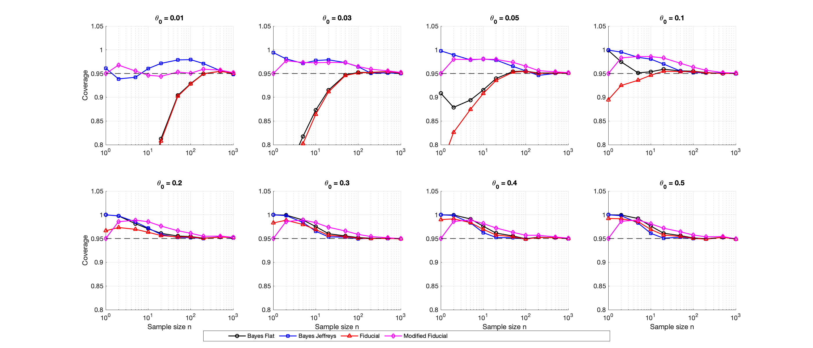
Since the inversion algorithm ignores evidence for values outside the parameter space, the normalization of the remaining pieces redistributes that missing mass among interior values, leading to under-coverage when the truth $(\theta_{0})$ is at or near the boundary. This issue is not unique to GFI, but can arise in any likelihood-based inferential procedure when the true parameter lies at or near the boundary of a constrained space. For example, in the triangular distribution, a Bayesian posterior proportional to the likelihood (i.e. using a flat prior) suffers from the same redistribution to the interior as the GFD, causing under-coverage near the boundary. This under-covering issue at the boundary is illustrated in the top row of Figure 2. Each panel reports the empirical coverage, based on $10,000$ replicates, of nominal $95\%$ two-sided generalized fiducial intervals and Bayesian posterior credible intervals across a range of sample sizes $n$, for a fixed true parameter value $\theta_{0}$. The panels in the top row of that figure correspond to parameter values near the boundary. The red and black lines correspond to the GFD approach and the Bayesian approach using a flat (uniform) prior, respectively, and are shown to under-cover at most sample sizes. For very large values of $n$, accurate coverage is achieved by both approaches, as expected from the corresponding Bernstein–von Mises results.

An appropriate frequentist correction to this issue is to treat evidence for values outside the parameter space as evidence that the true parameter lies at the boundary, and assign probability to the boundary points. In the Bayesian case, the Jeffreys prior is guaranteed to be first-order probability matching in the interior, and though not optimal at the boundaries, still puts relatively more weight towards the boundaries than a flat prior. Probability matching GFDs and exact coverage in single parameter models are discussed in Majumder and Hannig (2016). In this example, a compensation can be made at the boundaries in the fiducial case by the following modification of the inverse image (leading to exact coverage for $n=1$):

$$\tilde{G}^{-1}(u,y)=\begin{cases}1&u<y^{2}\\ \frac{y^{2}}{u}&y^{2}\leq u<y\\ 1-\frac{(1-y)^{2}}{1-u}&y\leq u\leq 1-(1-y)^{2}\\ 0&1-(1-y)^{2}<u.\end{cases}$$

For $n>1$, a boundary correction is applied whenever any observation $y_{i}$ would place $\theta_{0}$ outside the interior. Thus, the smallest $y_{i}^{2}$ for the upper boundary and smallest $(1-y_{i})^{2}$ for the lower boundary determine a threshold for placing $\theta_{0}$ at 1 or 0. Because the $u_{i}$ are uniform realizations, these values directly determine the probability mass assigned to the boundaries. The remaining probability over the interior is assigned to the original GFD. Formally, this gives

$$r^{\mathrm{mod}}(\theta\,|\,\mathbf{y})=\min_{i}(1-y_{i})^{2}\,\delta_{\{0\}}+\min_{i}y_{i}^{2}\,\delta_{\{1\}}+\Big(1-\min_{i}y_{i}^{2}-\min_{i}(1-y_{i})^{2}\Big)r(\theta\,|\,\mathbf{y}),$$

where $r(\theta\,|\,\mathbf{y})$ is the original (unmodified) GFD.

Asymptotic normality also holds for the modified GFD since

$$\left\lVert R^{\text{mod}}_{\boldsymbol{\theta}|\mathbf{y}}-R_{\boldsymbol{\theta}|\mathbf{y}}\right\rVert_{TV}\leq\min_{i}y_{i}^{2}+\min_{i}(1-y_{i})^{2},$$

where the upper bound vanishes to 0 as $n\to\infty$. To see this, note that the CDF on $y\in(0,\theta_{0}]$ is $F_{Y}(y)=y^{2}/\theta_{0}$. Then, we have

$$P_{\theta_{0}}(Y_{(1)}>\varepsilon)=(1-F_{Y}(\varepsilon))^{n}=\left(1-\frac{\varepsilon^{2}}{\theta_{0}}\right)^{n}\leq e^{-n\varepsilon^{2}/\theta_{0}}.$$

It follows that, for $\theta_{0}$ fixed, $\min_{i}y_{i}^{2}=O_{p}{(n^{-1/2})}$, and similarly, $\min_{i}(1-y_{i})^{2}=O_{p}{(n^{-1/2})}$.

Figure 3: Box-and-whisker plots of two-sided interval lengths for each method at various sample sizes, shown for a true parameter value near the boundary (top row) and in the interior (bottom row).

The blue and magenta lines in Figure 2 show coverage probabilities corresponding to the Jeffreys Bayesian and modified GFD methods, respectively, which give improved coverage over their alternative counterparts (Bayesian with flat prior and standard GFD) for parameter values near the boundary. Note that the modified GFD achieves exact coverage at $n=1$ (for all parameter values), as expected, while the Jeffreys Bayesian method is conservative there and, in general, more conservative at small sample sizes. Figure 3 shows box-and-whisker plots of the lengths of the two-sided generalized fiducial and Bayesian posterior credible intervals across sample sizes, for a true parameter value both near the boundary and in the interior. The standard GFD achieves the shortest intervals in general, and has competitive coverage at all sample sizes for interior parameter values, while the modified GFD achieves the best coverage near the boundary and competitive coverage at small sizes in general, but produces slightly wider intervals. The Bayesian approach with Jeffreys prior is most competitive at medium sample sizes for interior parameter values, but is conservative at small sample sizes. As expected from the asymptotic results, all four methods perform similarly for larger sample sizes. Table 1 in the supplementary material summarizes the empirical coverage and length of two-sided $95\%$ nominal intervals for each method at additional sample sizes and values of the true parameter.

Example 4.2.

As an example of a dependent data setting, we consider a stationary second-order autoregressive [AR(2)] time series model,

$$Y_{t}=\phi_{1}Y_{t-1}+\phi_{2}Y_{t-2}+\sigma\varepsilon_{t},\quad\varepsilon_{t}\stackrel{{\scriptstyle\text{iid}}}{{\sim}}N(0,1),$$

where the autoregressive coefficients $\boldsymbol{\phi}=(\phi_{1},\phi_{2})$ satisfy the stationarity conditions:

$$\phi_{1}+\phi_{2}<1,\hskip 2.84544pt\phi_{2}-\phi_{1}<1,\text{ and }|\phi_{2}|<1.$$

The results presented below extend naturally to any AR($p$) model; however, we restrict our attention to the case $p=2$ for simplicity and to provide a concrete illustration.

Following the approach in Box and Jenkins (1976), the likelihood function for this model can be expressed as

$$p_{\boldsymbol{\phi},\sigma^{2}}(y_{1},\dots,y_{T})=h(\boldsymbol{\phi},\sigma^{2})\ \times(\sigma^{2})^{-(T-2)/2}\times\exp\!\left\{-\frac{1}{2\sigma^{2}}\sum_{t=3}^{T}(y_{t}-\phi_{1}y_{t-1}-\phi_{2}y_{t-2})^{2}\right\},$$

$$\text{where }\quad h(\boldsymbol{\phi},\sigma^{2})=(\sigma^{2})^{-1}\lvert V^{-1}\rvert^{1/2}\exp\!\left\{-\frac{1}{2\sigma^{2}}(y_{1},y_{2})^{\prime}V^{-1}(y_{1},y_{2})\right\}$$

and

$$V^{-1}=\begin{pmatrix}1-\phi_{2}^{2}&-\phi_{1}(1+\phi_{2})\\ -\phi_{1}(1+\phi_{2})&1-\phi_{2}^{2}\end{pmatrix}.$$

Let $\boldsymbol{\theta}=(\phi_{1},\phi_{2},\sigma^{2})$, and let $P^{(T)}_{\boldsymbol{\theta}}$ denote the distribution of the full vector $(Y_{1},\dots,Y_{T})$ with stationary initial distribution for $(Y_{1},Y_{2})$. According to Kreiss (1987, 1990), the conditional distribution of $(Y_{3},\dots,Y_{T})$ given $(Y_{1},Y_{2})$ is locally asymptotically normal with central sequence

$$\Delta_{T,\boldsymbol{\theta}}=\frac{1}{\sqrt{T}}\begin{pmatrix}\displaystyle\frac{1}{\sigma^{2}}\sum_{t=3}^{T}(y_{t}-\phi_{1}y_{t-1}-\phi_{2}y_{t-2})\begin{pmatrix}y_{t-1}\\ y_{t-2}\end{pmatrix}\\[8.00003pt] \displaystyle\frac{1}{2\sigma^{4}}\sum_{t=3}^{T}\big[(y_{t}-\phi_{1}y_{t-1}-\phi_{2}y_{t-2})^{2}-\sigma^{2}\big]\end{pmatrix},$$

and asymptotic information matrix

$$I_{\boldsymbol{\theta}}=\begin{pmatrix}\frac{1}{\sigma^{2}}\begin{pmatrix}\gamma_{0}&\gamma_{1}\\ \gamma_{1}&\gamma_{0}\end{pmatrix}&0\\ 0&\frac{1}{2\sigma^{4}}\end{pmatrix},$$

where $\gamma_{k}=\mathrm{Cov}(Y_{t},Y_{t-k})$ under stationarity. Note that $h(\boldsymbol{\phi},\sigma^{2})$ is $O_{P^{(T)}_{\boldsymbol{\theta}}}(1)$ and is therefore negligible in the LAN expansion of the full likelihood.

A DGA for this model can be defined conditionally as:

$$G_{1}(\boldsymbol{\theta},\boldsymbol{\varepsilon})=y_{1}=\sqrt{\frac{1-\phi_{2}}{1+\phi_{2}}\frac{\sigma^{2}}{(1-\phi_{2})^{2}-\phi_{1}^{2}}}\varepsilon_{1},\qquad G_{2}(\boldsymbol{\theta},\boldsymbol{\varepsilon})=y_{2}=\frac{\phi_{1}}{1-\phi_{2}}y_{1}+\sqrt{\frac{\sigma^{2}}{1-\phi_{2}^{2}}}\varepsilon_{2},$$

and for $t\geq 3$,

$$G_{t}(\boldsymbol{\theta},\boldsymbol{\varepsilon})=y_{t}=\phi_{1}y_{t-1}+\phi_{2}y_{t-2}+\sigma\varepsilon_{t}.$$

Then, to derive the GFD, we invert the DGA to solve for the auxiliary variable, differentiate the data generating function $G(\boldsymbol{\varepsilon},\boldsymbol{\theta})$ with respect to the parameters, and substitute the inversions for $\varepsilon_{t}$. Details of that procedure are provided in the supplementary material.

Let $\mathcal{J}(\mathbf{y},\boldsymbol{\theta})=\nabla_{\boldsymbol{\theta}}G(\mathbf{u},\boldsymbol{\theta})\bigg|_{\boldsymbol{\varepsilon}=G^{-1}(\mathbf{y},\boldsymbol{\theta})}$ denote the gradient matrix with columns corresponding to $\phi_{1},\phi_{2},\sigma$ and recall that the Jacobian function in the fiducial solution can be expressed as

$$J(\mathbf{y},\boldsymbol{\theta})=\det\!\left(\frac{1}{T}\mathcal{J}(\mathbf{y},\boldsymbol{\theta})^{\top}\mathcal{J}(\mathbf{y},\boldsymbol{\theta})\right)^{1/2}.$$

We summarize computation of the Jacobian function here, with full details provided in the supplementary material. A factor of $1/\sigma$ appearing in the $\sigma$-column of $\mathcal{J}(\mathbf{y},\boldsymbol{\theta})$ can be factored out of the determinant; moreover, this column is a linear combination of the first two columns and $\mathbf{y}=(y_{1},y_{2},\ldots,y_{T})^{\top},$ so may be replaced by $\mathbf{y}$ in the determinant. Hence,

$$\tilde{\mathcal{J}}(\mathbf{y},\boldsymbol{\theta})=\begin{pmatrix}c_{1}y_{1}&d_{1}y_{1}&y_{1}\\[6.0pt] c_{2}y_{1}&d_{2}y_{1}+\phi_{2}y_{2}&y_{2}\\[6.0pt] y_{2}&y_{1}&y_{3}\\[6.0pt] y_{3}&y_{2}&y_{4}\\[6.0pt] \vdots&\vdots&\vdots\\[6.0pt] y_{T-1}&y_{T-2}&y_{T}\end{pmatrix},$$

where

$$c_{1}=\frac{\phi_{1}}{(1-\phi_{2})^{2}-\phi_{1}^{2}},\quad d_{1}=\frac{\phi_{1}^{2}+(1-\phi_{2})^{2}\phi_{2}}{(1-\phi_{2}^{2})\big((1-\phi_{2})^{2}-\phi_{1}^{2}\big)},\quad c_{2}=\frac{1}{1-\phi_{2}},\text{ and }d_{2}=\frac{\phi_{1}\phi_{2}}{(1-\phi_{2})^{2}}.$$

Thus, $J(\mathbf{y},\boldsymbol{\theta})=(\sigma\sqrt{T})^{-1}\det\!\left(\tilde{\mathcal{J}}^{\top}\tilde{\mathcal{J}}\right)^{1/2}.$

The supplementary material contains detailed verification of the conditions for Theorem 3.1 to show that, under the true parameter $\boldsymbol{\theta_{0}}$,

$$\left\lVert R_{\sqrt{T}(\bar{\boldsymbol{\Theta}}-\boldsymbol{\theta}_{0})\mid\mathbf{Y}}-N\big(I_{\boldsymbol{\theta}_{0}}^{-1}\Delta_{T,\boldsymbol{\theta}_{0}},I_{\boldsymbol{\theta}_{0}}^{-1}\big)\right\rVert_{TV}\;\;\overset{P_{\boldsymbol{\theta}_{0}}^{(T)}}{\longrightarrow}0.$$

The key reason these conditions hold despite the dependence between observations is that, as a consequence of stationarity, the autocovariances of observations from an AR(2) process decay exponentially fast. This exponential decay is used to establish a law of large numbers for the terms in the Jacobian function and the existence of uniformly exponentially consistent tests against local alternatives.

Figure 4: Kernel density estimates for the GFD (red) and Bayesian posterior with Jeffreys prior (blue) for the AR(2) model with true parameters $(\phi_{1}^{0},\phi_{2}^{0},\sigma^{0})=(0.5,-0.3,1)$. Black dashed curves show the corresponding normal approximations $N\big(I_{\boldsymbol{\theta}_{0}}^{-1}\Delta_{T,\boldsymbol{\theta}_{0}},I_{\boldsymbol{\theta}_{0}}^{-1}\big)$. Top and bottom rows correspond to sample sizes $n=50$ and $n=500$, respectively, with draws rescaled to the local scale; convergence to the normal approximation is evident as $n$ increases from $50$ to $500$.

We conducted a simulation study of the AR(2) process, using a Metropolis-within-Gibbs scheme to sample from both the GFD and the Bayesian posterior with Jeffreys prior for parameter estimation. The Fisher information in the Jeffreys prior is computed from the full likelihood including the initial observations; details are provided in the supplementary material. Figure 4 displays results from the simulation study, where each panel shows kernel density estimates for the GFD (red) and the Bayesian posterior (blue), with the corresponding normal approximations overlaid as black dashed curves. The top row corresponds to a sample size of $n=50$ and the bottom row to $n=500$, with data generated from the true parameter values $(\phi_{1}^{0},\phi_{2}^{0},\sigma^{0})=(0.5,-0.3,1)$. As in Figure 1, the kernel density estimates are computed after rescaling draws to the local scale, and the normal curve corresponds to $N\big(I_{\boldsymbol{\theta}_{0}}^{-1}\Delta_{T,\boldsymbol{\theta}_{0}},I_{\boldsymbol{\theta}_{0}}^{-1}\big)$, where $I_{\boldsymbol{\theta}_{0}}$ is the asymptotic information matrix given earlier. Convergence of the generalized fiducial and Bayesian densities to the normal approximation is observed as the sample size increases from $n=50$ to $n=500$.

Figure 5 plots the empirical coverage of nominal $1-\alpha$ two-sided generalized fiducial intervals and Bayesian posterior credible intervals for the AR true parameter $\phi_{1}^{0}$ across a range of $\alpha$, based on $M=10,000$ Monte Carlo experiments. The red points and lines correspond to coverage from the GFD, while the blue points and lines correspond to the Bayesian posterior. The black dashed line represents exact coverage. The top panel shows results for a sample of size $n=25$ and the bottom for $n=100$, with data again generated from the true parameters $(\phi_{1}^{0},\phi_{2}^{0},\sigma^{0})=(0.5,-0.3,1)$. Figure 6 and Figure 7 show analogous plots for the parameters $\phi_{2}^{0}$ and $\sigma^{0}$, respectively. For all parameters, Bayesian intervals tend to under-cover at the smaller sample size, but are close to nominal for $n=100$, while intervals from the GFD are closer to nominal in all cases.

Figure 5: Empirical coverage of two-sided GFD (red) and Bayesian intervals (blue) for the true AR parameter $\phi_{1}^{0}$ across nominal levels $1-\alpha$. Exact coverage indicated by a black dashed line. Top and bottom panels correspond to sample sizes $n=25$ and $n=100$, respectively, with data generated from true parameters $(\phi_{1}^{0},\phi_{2}^{0},\sigma^{0})=(0.5,-0.3,1)$. Note that Bayesian intervals tend to under-cover compared to the fiducial.

Figure 6: Same as Figure 5, for the AR parameter $\phi_{2}$.

Figure 7: Same as Figure 5, for $\sigma^{0}$. Under-coverage of Bayesian intervals is most obvious here.

This research was supported in part by the National Science Foundation under Grant No. DMS-1916115, DMS-2113404, and DMS-2210337.

5 Preliminaries

5.1 Notation

Before presenting the details of our theoretical results, we introduce additional notation used in the proofs that was not already defined in the main paper.

We denote the parameter $\boldsymbol{\theta}$ rescaled to the local parameter as $\mathbf{h}=\sqrt{n}(\boldsymbol{\theta}-\boldsymbol{\theta}_{0}).$ Let $\mathbf{H}_{n}=\mathbb{R}^{d}$ denote the space of local parameters and define the locally rescaled random variable

$$\bar{\mathbf{H}}_{n}=\sqrt{n}\,(\bar{\boldsymbol{\Theta}}-\boldsymbol{\theta}_{0}).$$

For $\mathbf{h}\in\mathbf{H}_{n}$, write the Jacobian appearing in the fiducial density under the original parameter $\boldsymbol{\theta}=\boldsymbol{\theta}_{0}+\mathbf{h}/\sqrt{n}$ $\boldsymbol{\theta}=\boldsymbol{\theta}_{0}+\mathbf{h}/\sqrt{n}$ as

$$J_{n}(\mathbf{h})=J(\mathbf{y},\boldsymbol{\theta}_{0}+\mathbf{h}/\sqrt{n}),$$

and denote the density of its limiting measure (in $n$), when it exists, under the original parameter by

$$\pi_{n}(\mathbf{h})=\pi(\boldsymbol{\theta}_{0}+\mathbf{h}/\sqrt{n}).$$

Let $\Pi_{n}$ denote the measure on $\mathbf{h}$ with density $\pi_{n}$ with respect to Lebesgue measure. For a measurable set $C\subset\mathbb{R}^{d}$, define the truncated and renormalized measure $\Pi_{n}^{C}$ by

$$\pi_{n}^{C}(\mathbf{h})=\frac{\mathbbm{1}_{C}(\mathbf{h})\pi_{n}(\mathbf{h})}{\Pi_{n}(C)}.$$

We denote the posterior distributions formed relative to $\Pi_{n}$ and $\Pi_{n}^{C}$ by $\Pi_{\bar{\mathbf{H}}_{n}\mid\mathbf{Y}}$ and $\Pi_{\bar{\mathbf{H}}_{n}\mid\mathbf{Y}}^{C}$, respectively.

Let $P_{n,\mathbf{h}}$ denote the distribution of $\mathbf{Y}$ under the original parameter $\boldsymbol{\theta}_{0}+\mathbf{h}/\sqrt{n}$, with density $p_{n,\mathbf{h}}(\mathbf{y})$ with respect to a dominating measure $\mu_{n}$. We use the notation $P_{n,\mathbf{0}}$ to denote the specific case $\boldsymbol{\theta}=\boldsymbol{\theta}_{0}.$ Define the probability measure

$$P_{n,C}=\int P_{n,\mathbf{h}}\,d\Pi_{n}^{C}(\mathbf{h})=\frac{1}{\Pi_{n}(C)}\int_{C}P_{n,\mathbf{h}}\,\pi_{n}(\mathbf{h})\,d\mathbf{h},$$

and write expectations with respect to $P_{n,C}$ as $E_{n,C}$.

Finally, define

$$R_{\sqrt{n}(\bar{\boldsymbol{\Theta}}-\boldsymbol{\theta}_{0})\mid\mathbf{Y}}=R_{\bar{\mathbf{H}}_{n}\mid\mathbf{Y}}$$

as the generalized fiducial distribution on the local parameter scale, and denote its truncation to $C$ by $R^{C}_{\bar{\mathbf{H}}_{n}\mid\mathbf{Y}}$, having density

$$r^{C}(\mathbf{h}\mid\mathbf{y})=\frac{\mathbbm{1}_{C}(\mathbf{h})\,p_{n,\mathbf{h}}(\mathbf{y})\,J_{n}(\mathbf{h})}{\int_{C}p_{n,\mathbf{g}}(\mathbf{y})\,J_{n}(\mathbf{g})\,d\mathbf{g}}.$$

6 Proofs

Proof of Theorem 3.1.

Let $C_{n}$ denote a ball centered at $0$ with radius $M_{n}\to\infty$. To establish convergence of the GFD to the normal distribution in total variation distance, we rely on the following decomposition:

$$\left\lVert R_{\bar{\mathbf{H}}_{n}|\mathbf{Y}}-N(I_{\boldsymbol{\theta}_{0}}^{-1}\Delta_{n,\boldsymbol{\theta}_{0}},I_{\boldsymbol{\theta}_{0}}^{-1})\right\rVert_{TV}\leq\left\lVert R_{\bar{\mathbf{H}}_{n}|\mathbf{Y}}^{C_{n}}-N^{C_{n}}(I_{\boldsymbol{\theta}_{0}}^{-1}\Delta_{n,\boldsymbol{\theta}_{0}},I_{\boldsymbol{\theta}_{0}}^{-1})\right\rVert_{TV}+\left\lVert R_{\bar{\mathbf{H}}_{n}|\mathbf{Y}}-R_{\bar{\mathbf{H}}_{n}|\mathbf{Y}}^{C_{n}}\right\rVert_{TV}\\ +\left\lVert N^{C_{n}}(I_{\boldsymbol{\theta}_{0}}^{-1}\Delta_{n,\boldsymbol{\theta}_{0}},I_{\boldsymbol{\theta}_{0}}^{-1})-N(I_{\boldsymbol{\theta}_{0}}^{-1}\Delta_{n,\boldsymbol{\theta}_{0}},I_{\boldsymbol{\theta}_{0}}^{-1})\right\rVert_{TV}.$$

The proof proceeds by controlling each term separately, which we organize into separate steps. In Step 1, we show convergence of the truncated GFD to the truncated normal distribution (the first term) using the LAN property. Step 2 relies on uniformly exponentially consistent tests for

$$H_{0}:\boldsymbol{\theta}=\boldsymbol{\theta}_{0}\qquad\text{versus}\qquad H_{1}:\|\boldsymbol{\theta}-\boldsymbol{\theta}_{0}\|\geq\varepsilon,$$

as guaranteed by Assumption 5 to show that the GFD has vanishing mass outside $C_{n}$ (second term). Since $M_{n}\to\infty$, the third term vanishes automatically.

Step 1: Convergence of the truncated GFD to the truncated normal.

First note that

$$\bigl\|R_{\bar{\mathbf{H}}_{n}|\mathbf{Y}}^{C_{n}}-N^{C_{n}}(I_{\boldsymbol{\theta}_{0}}^{-1}\Delta_{n,\boldsymbol{\theta}_{0}},I_{\boldsymbol{\theta}_{0}}^{-1})\bigr\|_{TV}\leq\bigl\|\Pi_{\bar{\mathbf{H}}_{n}|\mathbf{Y}}^{C_{n}}-N^{C_{n}}(I_{\boldsymbol{\theta}_{0}}^{-1}\Delta_{n,\boldsymbol{\theta}_{0}},I_{\boldsymbol{\theta}_{0}}^{-1})\bigr\|_{TV}+\bigl\|R_{\bar{\mathbf{H}}_{n}|\mathbf{Y}}^{C_{n}}-\Pi_{\bar{\mathbf{H}}_{n}|\mathbf{Y}}^{C_{n}}\bigr\|_{TV}.$$ (6.1)

Recall that for two probability measures $P,Q$ with densities $p,q$,

$$\|P-Q\|_{TV}=2\int\left(1-\frac{p}{q}\right)_{+}dQ.$$

To show the first term in (6.1) converges to 0 in $P_{n,\textbf{0}}$-probability, the argument follows exactly as in the Bayesian Bernstein-von Mises theorem. We present it here for completeness.

By Assumption 2, there exists $D_{n}>0$ such that $D_{n}\sqrt{n}\to\infty$ and

$$\sup_{\|\mathbf{q}\|\leq D_{n}\sqrt{n}}\left|\frac{J_{n}(\mathbf{q})}{\pi_{n}(\mathbf{q})}-1\right|=o_{P_{\theta_{0}}}(1).$$

Fix a ball $C$ centered at $0$ with radius $M<D_{n}\sqrt{n}$. Let $\phi_{n}$ denote the density of $N(I_{\boldsymbol{\theta}_{0}}^{-1}\Delta_{n,\boldsymbol{\theta}_{0}},I_{\boldsymbol{\theta}_{0}}^{-1})$ and define $\phi_{n}^{C}(\mathbf{h})=\mathbbm{1}_{C}(\mathbf{h})\phi_{n}(\mathbf{h})/\phi_{n}(C)$. Then,

$$\frac{1}{2}\bigl\|\Pi_{\mathbf{H}_{n}|\mathbf{Y}}^{C}-N^{C}(\Delta_{n,\boldsymbol{\theta}_{0}},I^{-1})\bigr\|_{TV} =\int\left(1-\frac{\phi_{n}^{C}(\mathbf{h})}{\dfrac{\mathbbm{1}_{C}(\mathbf{h})p_{n,\mathbf{h}}(\mathbf{y})\pi_{n}(\mathbf{h})}{\int_{C}p_{n,\mathbf{g}}(\mathbf{y})\pi_{n}(\mathbf{g})\,d\mathbf{g}}}\right)_{+}d\Pi_{\mathbf{H}_{n}|\mathbf{Y}}^{C}(\mathbf{h})$$

$$\leq\iint\left(1-\frac{\phi_{n}(\mathbf{h})p_{n,\mathbf{g}}(\mathbf{y})\pi_{n}(\mathbf{g})}{\phi_{n}(\mathbf{g})p_{n,\mathbf{h}}(\mathbf{y})\pi_{n}(\mathbf{h})}\right)_{+}\phi_{n}^{C}(\mathbf{g})\,d\mathbf{g}\,d\Pi_{\mathbf{H}_{n}|\mathbf{Y}}^{C}(\mathbf{h}),$$

where the last line follows by multiplying by $\phi_{n}^{C}(\mathbf{g})/\phi_{n}^{C}(\mathbf{g})$ and applying Jensen’s inequality.

Define

$$I(\mathbf{h},\mathbf{g},\mathbf{y})=\iint\left(1-\frac{\phi_{n}(\mathbf{h})p_{n,\mathbf{g}}(\mathbf{y})\pi_{n}(\mathbf{g})}{\phi_{n}(\mathbf{g})p_{n,\mathbf{h}}(\mathbf{y})\pi_{n}(\mathbf{h})}\right)_{+}\phi_{n}^{C}(\mathbf{g})\,d\mathbf{g}\,d\Pi_{\mathbf{H}_{n}|\mathbf{Y}}^{C}(\mathbf{h}).$$

We show $I(\mathbf{h},\mathbf{g},\mathbf{y})\to 0$ in $P_{n,C}$-mean. Using Bayes’ formula,

$$d\Pi_{\mathbf{H}_{n}|\mathbf{Y}}^{C}(\mathbf{h})\,dP_{n,C}(\mathbf{y})=p_{n,\mathbf{h}}(\mathbf{y})\pi_{n}^{C}(\mathbf{h})\,d\mathbf{h}\,d\mu_{n}(\mathbf{y}),$$

so

$$\int I(\mathbf{h},\mathbf{g},\mathbf{y})\,dP_{n,C}(\mathbf{y}) =\iiint\left(1-\frac{\phi_{n}(\mathbf{h})p_{n,\mathbf{g}}(\mathbf{y})\pi_{n}(\mathbf{g})}{\phi_{n}(\mathbf{g})p_{n,\mathbf{h}}(\mathbf{y})\pi_{n}(\mathbf{h})}\right)_{+}\phi_{n}^{C}(\mathbf{g})\,p_{n,\mathbf{h}}\pi_{n}^{C}(\mathbf{h})\,d\mathbf{g}\,d\mathbf{h}\,d\mu_{n}(\mathbf{y}).$$

Since $P_{n,\mathbf{h}}\triangleleft\triangleright P_{n,\mathbf{0}}$ and $C$ is bounded, $\phi_{n}^{C}$ and $\pi_{n}^{C}$ are contiguous with the uniform distribution on $C$, hence

$$\phi_{n}^{C}(\mathbf{g})\,p_{n,\mathbf{h}}(\mathbf{y})\pi_{n}^{C}(\mathbf{h})\triangleleft\triangleright\lambda^{C}(\mathbf{g})\,p_{n,\mathbf{0}}(\mathbf{y})\lambda^{C}(\mathbf{h}).$$

By continuity of $\pi$,

$$\frac{\pi_{n}(\mathbf{h})}{\pi_{n}(\mathbf{g})}\to 1,$$

and by LAN, as detailed in Lemma 6.2,

$$\frac{p_{n,\mathbf{g}}(\mathbf{y})\phi_{n}(\mathbf{h})}{p_{n,\mathbf{h}}(\mathbf{y})\phi_{n}(\mathbf{g})}\stackrel{{\scriptstyle P_{n,\textbf{0}}}}{{\to}}1.$$

Therefore the integrand converges to $0$ in $P_{n,\textbf{0}}$-probability for each g and h. Uniform integrability yields convergence in $P_{n,\mathbf{0}}$-mean for each fixed $\mathbf{h}$ and $\mathbf{g}$. By the dominated convergence theorem, this implies convergence in $\lambda^{C}(\mathbf{g})\,p_{n,\mathbf{0}}(\mathbf{y})\,\lambda^{C}(\mathbf{h})$-mean, and hence in probability, under this product measure. By contiguity, convergence in probability then also holds under $\phi_{n}^{C}(\mathbf{g})\,p_{n,\mathbf{h}}(\mathbf{y})\,\pi_{n}^{C}(\mathbf{h}).$ Again, uniform integrability implies convergence in $\phi_{n}^{C}(\mathbf{g})\,p_{n,\mathbf{h}}(\mathbf{y})\,\pi_{n}^{C}(\mathbf{h})$-mean, that is, in $P_{n,C}$-mean. Finally, convergence in $P_{n,\mathbf{0}}$-probability follows by contiguity, as in Lemma 6.1.

The second term in (6.1) is handled analogously. Indeed,

$$\frac{1}{2}\bigl\|R_{\bar{\mathbf{H}}_{n}|\mathbf{Y}}^{C_{n}}-\Pi_{\bar{\mathbf{H}}_{n}|\mathbf{Y}}^{C_{n}}\bigr\|_{TV}=\int\left(1-\frac{\mathbbm{1}_{C}(\mathbf{h})\,p_{n,\mathbf{h}}(\mathbf{y})J_{n}(\mathbf{h})/\int_{C}p_{n,\mathbf{g}}(\mathbf{y})J_{n}(\mathbf{g})\,d\mathbf{g}}{\mathbbm{1}_{C}(\mathbf{h})\,p_{n,\mathbf{h}}(\mathbf{y})\pi_{n}(\mathbf{h})/\int_{C}p_{n,\mathbf{g}}(\mathbf{y})\pi_{n}(\mathbf{g})\,d\mathbf{g}}\right)_{+}d\Pi_{\mathbf{H}_{n}|\mathbf{Y}}^{C}(\mathbf{h}).$$

Since $C$ is a ball around $\mathbf{0}$, Assumption 2 implies

$$\frac{\mathbbm{1}_{C}J_{n}(\mathbf{h})}{\mathbbm{1}_{C}\pi_{n}(\mathbf{h})}\stackrel{{\scriptstyle P_{n,\mathbf{0}}}}{{\longrightarrow}}1,$$

and

$$\frac{\int_{C}p_{n,\mathbf{g}}(\mathbf{y})\pi_{n}(\mathbf{g})\,d\mathbf{g}}{\int_{C}p_{n,\mathbf{g}}(\mathbf{y})J_{n}(\mathbf{g})\,d\mathbf{g}} =\frac{\int_{C}p_{n,\mathbf{g}}(\mathbf{y})\pi_{n}(\mathbf{g})\,d\mathbf{g}}{\int_{C}p_{n,\mathbf{g}}(\mathbf{y})J_{n}(\mathbf{g})\,d\mathbf{g}}=\frac{\int_{C}p_{n,\mathbf{g}}(\mathbf{y})\bigl(J_{n}(\mathbf{g})+(\pi_{n}(\mathbf{g})-J_{n}(\mathbf{g}))\bigr)\,d\mathbf{g}}{\int_{C}p_{n,\mathbf{g}}(\mathbf{y})J_{n}(\mathbf{g})\,d\mathbf{g}}$$

$$=1+\frac{\int_{C}p_{n,\mathbf{g}}(\mathbf{y})(\pi_{n}(\mathbf{g})-J_{n}(\mathbf{g}))\,d\mathbf{g}}{\int_{C}p_{n,\mathbf{g}}(\mathbf{y})J_{n}(\mathbf{g})\,d\mathbf{g}}\leq 1+\sup_{\mathbf{g}\in C}\frac{|\pi_{n}(\mathbf{g})-J_{n}(\mathbf{g})|}{J_{n}(\mathbf{g})}\stackrel{{\scriptstyle P_{n,\mathbf{0}}}}{{\longrightarrow}}1.$$

Hence, by the same $L_{1}$ argument as for the first term, we obtain

$$\bigl\|R_{\bar{\mathbf{H}}_{n}|\mathbf{Y}}^{C_{n}}-\Pi_{\bar{\mathbf{H}}_{n}|\mathbf{Y}}^{C_{n}}\bigr\|_{TV}\stackrel{{\scriptstyle P_{n,\mathbf{0}}}}{{\longrightarrow}}0.$$

Combining,

$$\bigl\|R_{\bar{\mathbf{H}}_{n}|\mathbf{Y}}^{C}-N^{C}(\Delta_{n,\boldsymbol{\theta}_{0}},I^{-1})\bigr\|_{TV}\overset{P_{n,\mathbf{0}}}{\longrightarrow}0.$$

This implies that there is some sequence $C_{n}$ with radius $M_{n}\to\infty$ such that:

$$\bigl\|R_{\bar{\mathbf{H}}_{n}|\mathbf{Y}}^{C_{n}}-N^{C_{n}}(\Delta_{n,\boldsymbol{\theta}_{0}},I^{-1})\bigr\|_{TV}\overset{P_{n,\mathbf{0}}}{\longrightarrow}0.$$

Step 2: Convergence of the GFD to the truncated GFD.

For any measurable set $B$ and a particular set $C$,

$$R_{\bar{\mathbf{H}}_{n}|\mathbf{Y}}(B)-R^{C}_{\bar{\mathbf{H}}_{n}|\mathbf{Y}}(B)=R_{\bar{\mathbf{H}}_{n}|\mathbf{Y}}(B\cap C^{c})-R^{C}_{\bar{\mathbf{H}}_{n}|\mathbf{Y}}(B)\,R_{\bar{\mathbf{H}}_{n}|\mathbf{Y}}(C^{c}).$$

Taking the supremum over $B$ yields

$$\|R_{\bar{\mathbf{H}}_{n}|\mathbf{Y}}-R^{C}_{\bar{\mathbf{H}}_{n}|\mathbf{Y}}\|_{TV}\leq 2\,R_{\bar{\mathbf{H}}_{n}|\mathbf{Y}}(C^{c}).$$

Hence it suffices to show that for any sequence $C_{n}=\{\|\mathbf{h}\|\leq M_{n}\}$ with $M_{n}\to\infty$,

$$R_{\bar{\mathbf{H}}_{n}|\mathbf{Y}}(C_{n}^{c})\overset{P_{n,\textbf{0}}}{\rightarrow}0.$$

We establish the stronger $L_{1}$ statement

$$\mathrm{E}_{n,C}\!\left[R_{\bar{\mathbf{H}}_{n}|\mathbf{Y}}(C_{n}^{c})\right]\to 0.$$

Let $\delta_{n}$ be exponentially consistent tests from Assumption 5. By contiguity, $\mathrm{E}_{n,C}(\delta_{n})\to 0$, and therefore

$$\mathrm{E}_{n,C}\!\left[R_{\bar{\mathbf{H}}_{n}|\mathbf{Y}}(C_{n}^{c})\right]=\mathrm{E}_{n,C}\!\left[R_{\bar{\mathbf{H}}_{n}|\mathbf{Y}}(C_{n}^{c})(1-\delta_{n}(\mathbf{Y}))\right]+o(1).$$

By Assumption 2, there exists $D_{n}>0$ such that $D_{n}\sqrt{n}\to\infty$ and

$$\sup_{\|\mathbf{q}\|\leq D_{n}\sqrt{n}}\left|\frac{J_{n}(\mathbf{q})}{\pi_{n}(\mathbf{q})}-1\right|=o_{P_{\theta_{0}}}(1).$$

Define

$$S_{1}:=\{M_{n}\leq\|\mathbf{h}\|\leq D_{n}\sqrt{n}\},\qquad S_{2}:=\{\|\mathbf{h}\|>D_{n}\sqrt{n}\},$$

and write

$$\mathrm{E}_{n,C}\!\left[R_{\bar{\mathbf{H}}_{n}|\mathbf{Y}}(C_{n}^{c})(1-\delta_{n}(\mathbf{Y}))\right]=I_{1}(\mathbf{h},\mathbf{g},\mathbf{y})+I_{2}(\mathbf{h},\mathbf{g},\mathbf{y}),$$

where

$$I_{i}(\mathbf{h},\mathbf{g},\mathbf{y})=\int\int_{C}\int_{S_{i}}\frac{p_{n,\mathbf{h}}(\mathbf{y})J_{n}(\mathbf{h})}{\int p_{n,\mathbf{q}}(\mathbf{y})J_{n}(\mathbf{q})\,d\mathbf{q}}(1-\delta_{n}(\mathbf{y}))\frac{p_{n,\mathbf{g}}(\mathbf{y})\pi_{n}(\mathbf{g})}{\Pi_{n}(C)}\,d\mathbf{h}\,d\mathbf{g}\,d\mu_{n}(\mathbf{y}).$$

Recall that $J_{n}(\mathbf{q})=J_{n}(\mathbf{Y},\mathbf{q}).$ Let $\varepsilon_{1}>0$ and define also

$$\mathcal{E}_{n}(\mathbf{Y}):=\left\{\omega:\sup_{\|\mathbf{q}\|\leq D_{n}\sqrt{n}}\left|\frac{J_{n}(\mathbf{Y}(\omega),\mathbf{q})}{\pi_{n}(\mathbf{q})}-1\right|\leq\varepsilon_{1}\right\}.$$

Then, there exists $N_{1}$ such that for $n\geq N_{1}$,

$$I_{1} =\int\int_{C}\int_{S_{1}}\frac{p_{n,\mathbf{h}}(\mathbf{y})J_{n}(\mathbf{h})}{\int p_{n,\mathbf{q}}(\mathbf{y})J_{n}(\mathbf{q})\,d\mathbf{q}}\frac{\pi_{n}(\mathbf{h})}{\pi_{n}(\mathbf{h})}(1-\delta_{n}(\mathbf{y}))\frac{p_{n,\mathbf{g}}(\mathbf{y})J_{n}(\mathbf{g})}{\Pi_{n}(C)}\frac{J_{n}(\mathbf{h})}{J_{n}(\mathbf{h})}\,\mathbbm{1}_{\mathcal{E}_{n}}\,d\mathbf{h}\,d\mathbf{g}\,d\mu_{n}(\mathbf{y})$$

$$\quad\quad+\underbrace{\int\int_{C}\int_{S_{1}}\frac{p_{n,\mathbf{h}}(\mathbf{y})J_{n}(\mathbf{h})}{\int p_{n,\mathbf{q}}(\mathbf{y})J_{n}(\mathbf{q})\,d\mathbf{q}}(1-\delta_{n}(\mathbf{y}))\frac{p_{n,\mathbf{g}}(\mathbf{y})\pi_{n}(\mathbf{g})}{\Pi_{n}(C)}\mathbbm{1}_{\mathcal{E}_{n}^{c}}\,d\mathbf{h}\,d\mathbf{g}\,d\mu_{n}(\mathbf{y})}_{=:R_{1}}$$

$$\leq(1+\varepsilon_{1})^{2}\int\int_{C}\int_{S_{1}}\frac{p_{n,\mathbf{h}}(\mathbf{y})\pi_{n}(\mathbf{h})}{\Pi_{n}(C)}(1-\delta_{n}(\mathbf{y}))\frac{p_{n,\mathbf{g}}(\mathbf{y})J_{n}(\mathbf{g})}{\int p_{n,\mathbf{q}}(\mathbf{y})J_{n}(\mathbf{q})\,d\mathbf{q}}\,\mathbbm{1}_{\mathcal{E}_{n}}\,d\mathbf{h}\,d\mathbf{g}\,d\mu_{n}(\mathbf{y})+R_{1}.$$

Here, we have used the fact that once $\mathbf{Y}=\mathbf{y}$ is fixed (i.e., $\omega$ is fixed in the probability space), the indicator $\mathbbm{1}_{\mathcal{E}_{n}(\mathbf{Y})}$ takes the same value for all $\mathbf{h}$ and $\mathbf{g}$. Hence, on the event $\mathcal{E}_{n}$, both ratios $J_{n}(\mathbf{h})/\pi_{n}(\mathbf{h})$ and $J_{n}(\mathbf{g})/\pi_{n}(\mathbf{g})$ are bounded by $1+\varepsilon_{1}$ uniformly over the corresponding domains. The complement of $\mathcal{E}_{n}$ contributes a remainder term $\varepsilon_{2}$, which can be made arbitrarily small in probability. To see this, let $\varepsilon_{2}>0$ and observe that there exists $N_{2}$ such that $n\geq N_{2}$,

$$R_{1}=\mathrm{E}_{n,C}\Bigg(\int_{S_{1}}\frac{p_{n,\mathbf{h}}(\mathbf{Y})J_{n}(\mathbf{h})}{\int p_{n,\mathbf{q}}(\mathbf{Y})J_{n}(\mathbf{q})\,d\mathbf{q}}(1-\delta_{n}(\mathbf{Y}))\mathbbm{1}_{\mathcal{E}_{n}^{c}}\,d\mathbf{h}\Bigg)\leq P_{n,C}\Big(\sup_{\|\mathbf{q}\|\leq D_{n}\sqrt{n}}\left|\frac{J_{n}(\mathbf{q})}{\pi_{n}(\mathbf{q})}-1\right|>\epsilon_{1}\Big)<\epsilon_{2},$$

where the final inequality follows from contiguity.

Then, for $n\geq\max(N_{1},N_{2})$, we proceed in three steps. First, applying the preceding results derived on the event $\mathcal{E}_{n}$, we obtain

$$I_{1}(\mathbf{h},\mathbf{g},\mathbf{y}) \leq(1+\varepsilon_{1})^{2}\int\int_{C}\int_{S_{1}}\frac{p_{n,\mathbf{h}}(\mathbf{y})\pi_{n}(\mathbf{h})}{\Pi_{n}(C)}(1-\delta_{n}(\mathbf{y}))\frac{p_{n,\mathbf{g}}(\mathbf{y})J_{n}(\mathbf{g})}{\int p_{n,\mathbf{q}}(\mathbf{y})J_{n}(\mathbf{q})\,d\mathbf{q}}\,\mathbbm{1}_{\mathcal{E}_{n}}\,d\mathbf{h}\,d\mathbf{g}\,d\mu_{n}(\mathbf{y})+\varepsilon_{2}.$$

Second, since $\mathbbm{1}_{\mathcal{E}_{n}}\leq 1$, enlarging the domain gives

$$\leq(1+\varepsilon_{1})^{2}\int\int_{C}\int_{S_{1}}\frac{p_{n,\mathbf{h}}(\mathbf{y})\pi_{n}(\mathbf{h})}{\Pi_{n}(C)}(1-\delta_{n}(\mathbf{y}))\frac{p_{n,\mathbf{g}}(\mathbf{y})J_{n}(\mathbf{g})}{\int p_{n,\mathbf{q}}(\mathbf{y})J_{n}(\mathbf{q})\,d\mathbf{q}}\,d\mathbf{h}\,d\mathbf{g}\,d\mu_{n}(\mathbf{y})+\varepsilon_{2}.$$

Third, applying Tonelli’s theorem to interchange the order of integration,

$$=(1+\varepsilon_{1})^{2}\int\int_{S_{1}}\int_{C}\frac{p_{n,\mathbf{h}}(\mathbf{y})\pi_{n}(\mathbf{h})}{\Pi_{n}(C)}(1-\delta_{n}(\mathbf{y}))\frac{p_{n,\mathbf{g}}(\mathbf{y})J_{n}(\mathbf{g})}{\int p_{n,\mathbf{q}}(\mathbf{y})J_{n}(\mathbf{q})\,d\mathbf{q}}\,d\mathbf{g}\,d\mathbf{h}\,d\mu_{n}(\mathbf{y}).$$

Finally, since

$$\frac{\int_{C}p_{n,\mathbf{g}}(\mathbf{y})J_{n}(\mathbf{g})\,d\mathbf{g}}{\int p_{n,\mathbf{q}}(\mathbf{y})J_{n}(\mathbf{q})\,d\mathbf{q}}\leq 1,$$

we obtain

$$I_{1}(\mathbf{h},\mathbf{g},\mathbf{y})\leq\frac{(1+\varepsilon_{1})^{2}}{\Pi_{n}(C)}\int_{S_{1}}\mathrm{E}_{n,\mathbf{h}}(1-\delta_{n}(\mathbf{Y}))\,\pi_{n}(\mathbf{h})\,d\mathbf{h}+\varepsilon_{2}.$$

By Assumption 3, there is $\rho\leq 1$ small enough such that $\pi(\boldsymbol{\theta})$ is uniformly bounded by a constant $c_{1}$ on $\|\boldsymbol{\theta}-\boldsymbol{\theta}_{0}\|\leq\rho$. Recall that $d$ denotes the dimension of $\boldsymbol{\Theta}$ and note that $\Pi_{n}(C)>\frac{c_{2}}{\sqrt{n}^{d}}$. Then, since the tests are uniformly exponentially consistent,

$$I_{1}(\mathbf{h},\mathbf{g},\mathbf{y}) \leq(1+\varepsilon_{1})^{2}\,c_{2}\,\sqrt{n}^{d}\int_{M_{n}\leq\left\lVert\textbf{h}\right\rVert\leq D_{n}\sqrt{n}}\pi_{n}(\mathbf{h})\,e^{-c_{3}(\left\lVert\textbf{h}^{2}\right\rVert\wedge n)}\,d\textbf{h}+\varepsilon_{2}$$

$$\leq(1+\varepsilon_{1})^{2}\,c_{2}\,\sqrt{n}^{d}\int_{M_{n}\leq\left\lVert\textbf{h}\right\rVert\leq D_{n}\sqrt{n}}\frac{c_{4}}{\sqrt{n}^{d}}c_{2}\,e^{-c_{3}(\left\lVert\textbf{h}^{2}\right\rVert\wedge n)}\,d\textbf{h}+\varepsilon_{2}$$

$$\leq(1+\varepsilon_{1})^{2}\,c_{5}\int_{M_{n}\leq\left\lVert\textbf{h}\right\rVert}e^{-c_{3}(\left\lVert\textbf{h}^{2}\right\rVert)}\,d\textbf{h}+\varepsilon_{2}\rightarrow 0\text{ as }n\to\infty,\,\,\varepsilon_{1}\to 0,\,\,\varepsilon_{2}\to 0.$$

Next consider $I_{2}(\mathbf{h},\mathbf{g},\mathbf{y})$. By a similar argument as before,

$$I_{2}(\mathbf{h},\mathbf{g},\mathbf{y})\leq(1+\varepsilon_{3})\int\int_{C}\int_{S_{2}}\frac{p_{n,\mathbf{h}}(\mathbf{y})J_{n}(\mathbf{h})}{\Pi_{n}(C)}(1-\delta_{n})\frac{p_{n,\mathbf{g}}(\mathbf{y})J_{n}(\mathbf{g})}{\int p_{n,\mathbf{q}}(\mathbf{y})J_{n}(\mathbf{q})\,d\mathbf{q}}\,d\mathbf{h}\,d\mathbf{g}\,d\mu_{n}(\mathbf{y})+\varepsilon_{4}.$$

By Assumption 4, write $p_{n,\mathbf{h}}(\mathbf{y})=p_{n,\mathbf{h}}^{1}(\mathbf{y})p_{n,\mathbf{h}}^{2}(\mathbf{y})$ and take $\gamma_{n}(\mathbf{h})$ such that

$$P_{\boldsymbol{\theta}_{0}}\big(p_{n,\mathbf{h}}^{2}(\mathbf{y})J_{n}(\mathbf{h})I_{\{\left\lVert\mathbf{h}\right\rVert>D_{n}\}}{\leq}\gamma(\mathbf{h})\big)\rightarrow 1.$$

Then, again applying Tonelli’s theorem and the bounds arising from $\Pi_{n}(C)>\frac{c_{2}}{\sqrt{n}^{d}}$ and exponential consistency,

$$I_{2}(\mathbf{h},\mathbf{g},\mathbf{y}) \leq(1+\varepsilon_{3})\int\int_{C}\int_{S_{2}}\dfrac{p_{n,\mathbf{h}}^{1}(\mathbf{y})\,\gamma_{n}(\mathbf{h})}{\Pi_{n}(C)}(1-\delta_{n}(\mathbf{y}))\dfrac{p_{n,\mathbf{g}}(\mathbf{y})J_{n}(\mathbf{g})}{\int p_{n,\mathbf{q}}(\mathbf{y})J_{n}(\mathbf{q})\,d\mathbf{q}}\,d\mathbf{h}\,d\mathbf{g}\,d\mu_{n}(\mathbf{y})+\varepsilon_{4}+(1+\varepsilon_{3})\varepsilon_{5}$$

$$\leq(1+\varepsilon_{3})\,\frac{1}{\Pi_{n}(C)}\int\int_{S_{2}}p_{n,\mathbf{h}}^{1}(\mathbf{y})\,\gamma_{n}(\mathbf{h})\,d\mathbf{h}\,d\mu_{n}(\mathbf{y})+\varepsilon_{4}+(1+\varepsilon_{3})\varepsilon_{5}$$

$$\leq(1+\varepsilon_{3})\,c_{2}\,\sqrt{n}^{d}\int_{\|\mathbf{h}\|>D_{n}\sqrt{n}}\mathrm{E}_{n,\mathbf{h}}^{1}(1-\delta_{n}(\mathbf{Y}))\gamma_{n}(\mathbf{h})\,d\mathbf{h}+\varepsilon_{4}+(1+\varepsilon_{3})\varepsilon_{5}$$

$$\leq(1+\varepsilon_{3})\,c_{2}\,\sqrt{n}^{d}e^{-c_{3}\rho^{2}n}+\varepsilon_{4}+(1+\varepsilon_{3})\varepsilon_{5}\rightarrow 0,\text{ as }n\to\infty,\,\,\varepsilon_{3},\varepsilon_{4},\varepsilon_{5}\to 0.$$

Combining the computations for $I_{1}(\mathbf{h},\mathbf{g},\mathbf{y})$ and $I_{2}(\mathbf{h},\mathbf{g},\mathbf{y})$,

$$\mathrm{E}_{n,C}\!\left[R_{\bar{\mathbf{H}}_{n}|\mathbf{Y}}(C_{n}^{c})(1-\delta_{n}(\mathbf{Y}))\right]\to 0,$$

and hence

$$\mathrm{E}_{n,C}\!\left[R_{\bar{\mathbf{H}}_{n}|\mathbf{Y}}(C_{n}^{c})\right]\to 0.$$

By Lemma 6.1, this implies

$$R_{\bar{\mathbf{H}}_{n}|\mathbf{Y}}(C_{n}^{c})\overset{P_{n,\textbf{0}}}{\rightarrow}0.$$

∎

Lemma 6.1.

Under Assumptions 1-3, given an arbitrary compact set $C\subset\mathbb{R}^{d}$,

$$P_{n,\textbf{0}}\lhd\rhd P_{n,C}.$$

Proof.

Suppose $P_{n,\textbf{0}}(A_{n})\rightarrow 0$ for some set $A_{n}$. A well-known fact under LAN is that for every h, $P_{n,\textbf{0}}\lhd\rhd P_{n,\textbf{h}}$. Thus, by contiguity, $P_{n,\textbf{h}}(A_{n})\rightarrow 0$ for any $\textbf{h}\in C$. Note that

$$P_{n,C}(A_{n})=\int_{C}P_{n,\textbf{h}}(A_{n})\pi_{n}^{C}(\textbf{h})d\textbf{h}.$$

Since $|P_{n,\textbf{h}}(A_{n})|\leq 1$ for all h, we can apply DCT to get $P_{n,C}(A_{n})\rightarrow 0.$

Now suppose $P_{n,C}(A_{n})\rightarrow 0$ for some $A_{n}$. Let $\textbf{h}_{n}\in C$ such that $P_{n,\textbf{h}_{n}}(A_{n})\leq P_{n,C}(A_{n})$. Thus, $P_{n,\textbf{h}_{n}}(A_{n})\rightarrow 0$ and it follows by contiguity $P_{n,\textbf{0}}(A_{n})\rightarrow 0$.

∎

Lemma 6.2.

Suppose Assumptions 1-3 hold. Let $\textbf{h},\textbf{g}\in\textbf{H}_{n}$ be distinct local alternatives. Then, $\dfrac{p_{n,\textbf{h}}(\textbf{y})\phi_{n}(\textbf{g})}{p_{n,\textbf{g}}(\textbf{y})\phi_{n}(\textbf{h})}\rightarrow 1$ in $P_{n,\textbf{h}}$.

Proof.

By the LAN property that follows from Assumption 1,

$$\dfrac{p_{n,\textbf{h}}(\textbf{y})\phi_{n}(\textbf{g})}{p_{n,\textbf{g}}(\textbf{y})\phi_{n}(\textbf{h})} =\dfrac{\dfrac{p_{n,\textbf{h}}(\textbf{y})}{p_{n,\textbf{0}}(\textbf{y})}}{\dfrac{p_{n,\textbf{g}}(\textbf{y})}{p_{n,\textbf{0}}(\textbf{y})}}\cdot\dfrac{\phi_{n}(\textbf{g})}{\phi_{n}(\textbf{h})}$$

$$=\dfrac{\exp\left(\textbf{h}^{\top}\Delta_{n,\boldsymbol{\theta}}-\dfrac{1}{2}\textbf{h}^{\top}I_{\boldsymbol{\theta}_{0}}\textbf{h}+o_{p_{n,\textbf{0}}}(1)\right)}{\exp\left(\textbf{g}^{\top}\Delta_{n,\boldsymbol{\theta}}-\dfrac{1}{2}\textbf{g}^{\top}I_{\boldsymbol{\theta}_{0}}\textbf{g}+o_{p_{n,\textbf{0}}}(1)\right)}\cdot\dfrac{\exp\left(-\dfrac{1}{2}\left(\textbf{g}-\Delta_{n,\boldsymbol{\theta}_{0}}\right)^{\top}I_{\boldsymbol{\theta}_{0}}(\textbf{g}-\Delta_{n,\boldsymbol{\theta}_{0}})\right)}{\exp\left(-\dfrac{1}{2}\left(\textbf{h}-\Delta_{n,\boldsymbol{\theta}_{0}}\right)^{\top}I_{\boldsymbol{\theta}_{0}}(\textbf{h}-\Delta_{n,\boldsymbol{\theta}_{0}})\right)}$$

$$=\dfrac{\exp\left(\textbf{h}^{\top}\Delta_{n,\boldsymbol{\theta}}-\dfrac{1}{2}\textbf{h}^{\top}I_{\boldsymbol{\theta}_{0}}\textbf{h}+o_{p_{n,\textbf{0}}}(1)\right)}{\exp\left(\textbf{g}^{\top}\Delta_{n,\boldsymbol{\theta}}-\dfrac{1}{2}g^{\top}I_{\boldsymbol{\theta}_{0}}\textbf{g}+o_{p_{n,\textbf{0}}}(1)\right)}\cdot\dfrac{\exp\left(-\dfrac{1}{2}\textbf{g}^{\top}I_{\boldsymbol{\theta}_{0}}\textbf{g}\right)}{\exp\left(-\dfrac{1}{2}\textbf{h}^{\top}I_{\boldsymbol{\theta}_{0}}\textbf{h}\right)}\cdot\dfrac{\exp\left(\dfrac{1}{\sqrt{n}}\textbf{g}^{\top}\Delta_{n,\boldsymbol{\theta}})\right)}{\exp\left(\dfrac{1}{\sqrt{n}}\textbf{h}^{\top}\Delta_{n,\boldsymbol{\theta}}\right)}$$

$$=\dfrac{e^{o_{P_{n,\textbf{0}}}(1)}}{e^{o_{P_{n,\textbf{0}}}(1)}}\stackrel{{\scriptstyle P_{n,\textbf{0}}}}{{\rightarrow}}1.$$

Since $P_{n,\textbf{0}}\lhd\rhd P_{n,\textbf{h}}$, it follows that $\dfrac{p_{n,\textbf{h}}(\textbf{y})\phi_{n}(\textbf{g})}{p_{n,\textbf{g}}(\textbf{y})\phi_{n}(\textbf{h})}\stackrel{{\scriptstyle P_{n,\textbf{h}}}}{{\rightarrow}}1$. ∎

7 Example 4.1

Below are the details for deriving the generalized fiducial solution and verifying each assumption of Theorem 3.1 for the triangular distribution example. Recall that probability density function for this distribution is given in Equation 4.1.

To derive the generalized fiducial solution, note that the cumulative distribution function (CDF) of the triangular distribution on $(0,1)$ with parameter $\theta$ is

$$F_{Y}(y)=0\cdot I_{(-\infty,0)}(y)+\dfrac{y^{2}}{\theta}I_{(0,\theta]}(y)+(1-\dfrac{(1-y)^{2}}{(1-\theta)}I_{[\theta,1)}(y)+1\cdot I_{[1,\infty)}(y).$$

We will use the inverse of the CDF as a DGA $\mathbf{Y}=G(\mathbf{U},\theta)$:

$$Y_{i}=\sqrt{U_{i}\theta}\hskip 1.42271ptI_{(0,\theta]}(U_{i})+(1-\sqrt{(1-U_{i})(1-\theta)}\hskip 1.42271ptI_{(\theta,1)}(U_{i})),\quad i=1,\ldots,n,$$ (7.1)

where $\textbf{U}=(U_{1},\ldots,U_{n})$ are i.i.d uniform distribution on the interval $(0,1)$.

The gradient of $G(\textbf{u},\theta)$ with respect to $\theta$ at $\textbf{u}=G^{-1}(\textbf{y},\theta)$ takes the form

$$\nabla_{\theta}G(\textbf{u},\theta)\Big|_{\textbf{u}=G^{-1}(\textbf{y},\theta)}=\begin{pmatrix}\frac{y_{1}}{2\theta}I_{(0,\theta]}(y_{1})+\frac{1-y_{1}}{2(1-\theta)}I_{(\theta,1)}(y_{1})\\ \vdots\\ \frac{y_{n}}{2\theta}I_{(0,\theta]}(y_{n})+\frac{1-y_{n}}{2(1-\theta)}I_{(\theta,1)}(y_{n})\end{pmatrix}.$$

Consequently, the Jacobian function is

$$J(\textbf{y},\theta)=\left(\frac{1}{n}\sum_{i=1}^{n}\left(\frac{y_{i}}{2\theta}\right)^{2}I_{(0,\theta]}(y_{i})+\frac{1}{n}\sum_{i=1}^{n}\left(\frac{1-y_{i}}{2(1-\theta)}\right)^{2}I_{(\theta,1)}(y_{i})\right)^{1/2}.$$ (7.2)

Assumption 1 (Local asymptotic normality). Since the data are i.i.d., it suffices to show that the model is differentiable in quadratic mean, i.e. we aim to show that

$$\int_{0}^{1}\left(\sqrt{p_{\theta+h}}-\sqrt{p_{\theta}}-\frac{1}{2}h\dot{\ell}_{\theta}\sqrt{p_{\theta}}\right)^{2}dy=o(h^{2}).$$

Substituting $p_{\theta}$ and $p_{\theta+h}$ for the triangular density yields

$$\int_{0}^{\theta}\!\!\left(\sqrt{\tfrac{2y}{\theta+h}}-\sqrt{\tfrac{2y}{\theta}}+\tfrac{1}{2}h\tfrac{1}{\theta}\sqrt{\tfrac{2y}{\theta}}\right)^{2}dy+\int_{\theta}^{\theta+h}\!\!\left(\sqrt{\tfrac{2y}{\theta+h}}-\sqrt{\tfrac{2-2y}{1-\theta}}-\tfrac{1}{2}h\tfrac{1}{1-\theta}\sqrt{\tfrac{2-2y}{1-\theta}}\right)^{2}dy$$

$$\qquad+\int_{\theta+h}^{1}\!\!\left(\sqrt{\tfrac{2-2y}{1-(\theta+h)}}-\sqrt{\tfrac{2-2y}{1-\theta}}-\tfrac{1}{2}h\tfrac{1}{1-\theta}\sqrt{\tfrac{2-2y}{1-\theta}}\right)^{2}dy.$$

It is straightforward to see show that the first and third integrals are $o(h^{2})$ from direct expansion. For the middle integral, the integrand is monotone in $y$; evaluating at the endpoints and applying a second-order Taylor expansion of the square-root terms around $h=0$ gives an upper bound of order $o(h^{2})$. Hence, the experiment is differentiable in quadratic mean (DQM).

Assumptions 2 (Convergence of Jacobian function in GF density) and 3 (Mass of limiting measure). From (7.2),

$$J(\mathbf{y},\theta)=\left(\frac{1}{n}\sum_{i=1}^{n}\Big[\!\left(\tfrac{y_{i}}{2\theta}\right)^{2}I_{(0,\theta]}(y_{i})+\left(\tfrac{1-y_{i}}{2(1-\theta)}\right)^{2}I_{(\theta,1)}(y_{i})\!\Big]\right)^{1/2}.$$

Each summand has finite variance (e.g., $\mathrm{E}[(Y/2\theta)^{4}I_{(0,\theta]}(Y)]=\theta/48$ and $\mathrm{E}[((1-Y)/2(1-\theta))^{4}I_{(\theta,1)}(Y)]=(1-\theta)/48$), so by the law of large numbers and the continuous mapping theorem,

$$J(\mathbf{y},\theta)\to\Big(\tfrac{\theta}{8}+\tfrac{1-\theta}{8}\Big)^{1/2}=\sqrt{\tfrac{1}{8}}.$$

Thus, for large $n$, the generalized fiducial distribution behaves similarly to a Bayesian posterior under a flat prior.

Assumption 4 (Likelihood splitting). Let $p^{1}_{\theta}=p_{\theta}$ and $p^{2}_{\theta}=1$. Because $J(\mathbf{y},\theta)\leq 1/4$, choosing $\gamma(\theta)=1$ ensures $p^{2}_{\theta}(\mathbf{y})J(\mathbf{y},\theta)\leq\gamma(\theta)$.

Assumption 5 (Exponentially consistent tests). Since the model is i.i.d., it suffices to verify the existence of uniformly consistent estimators. This follows directly from Lemma 7.6 in van der Vaart (1998).

	$\theta$
$n$	0.01	0.03	0.05	0.10	0.20	0.30	0.40	0.50
Generalized Fiducial 95% CI
1	0.298 (0.781)	0.603 (0.793)	0.753 (0.802)	0.895 (0.82)	0.966 (0.841)	0.983 (0.852)	0.990 (0.858)	0.992 (0.86)
2	0.389 (0.75)	0.710 (0.758)	0.826 (0.766)	0.925 (0.783)	0.973 (0.81)	0.989 (0.828)	0.992 (0.839)	0.992 (0.843)
5	0.557 (0.589)	0.802 (0.605)	0.875 (0.619)	0.936 (0.65)	0.970 (0.698)	0.980 (0.731)	0.984 (0.75)	0.986 (0.757)
10	0.689 (0.394)	0.864 (0.417)	0.908 (0.438)	0.946 (0.483)	0.963 (0.553)	0.969 (0.6)	0.969 (0.628)	0.969 (0.636)
20	0.808 (0.229)	0.911 (0.256)	0.935 (0.28)	0.955 (0.33)	0.956 (0.404)	0.957 (0.453)	0.957 (0.482)	0.957 (0.491)
50	0.902 (0.107)	0.946 (0.133)	0.953 (0.155)	0.954 (0.198)	0.953 (0.254)	0.954 (0.287)	0.954 (0.304)	0.955 (0.31)
100	0.928 (0.0611)	0.951 (0.0843)	0.955 (0.102)	0.954 (0.136)	0.953 (0.175)	0.951 (0.197)	0.949 (0.209)	0.951 (0.214)
200	0.949 (0.0373)	0.952 (0.0563)	0.950 (0.0699)	0.952 (0.0932)	0.950 (0.121)	0.950 (0.137)	0.953 (0.145)	0.949 (0.148)
500	0.955 (0.0213)	0.954 (0.0341)	0.951 (0.0424)	0.950 (0.0565)	0.953 (0.0742)	0.950 (0.0841)	0.952 (0.0897)	0.953 (0.0916)
1000	0.950 (0.0144)	0.951 (0.0233)	0.951 (0.0291)	0.950 (0.0392)	0.952 (0.0516)	0.949 (0.0588)	0.950 (0.0626)	0.949 (0.0639)
Modified Generalized Fiducial 95% CI
1	0.950 (0.798)	0.950 (0.814)	0.950 (0.83)	0.950 (0.87)	0.950 (0.922)	0.950 (0.941)	0.950 (0.948)	0.950 (0.951)
2	0.968 (0.816)	0.977 (0.83)	0.980 (0.844)	0.983 (0.88)	0.986 (0.935)	0.986 (0.958)	0.986 (0.968)	0.986 (0.971)
5	0.955 (0.656)	0.973 (0.682)	0.980 (0.706)	0.986 (0.764)	0.989 (0.862)	0.989 (0.91)	0.989 (0.933)	0.989 (0.939)
10	0.946 (0.426)	0.973 (0.457)	0.980 (0.487)	0.986 (0.562)	0.986 (0.709)	0.984 (0.804)	0.982 (0.85)	0.981 (0.865)
20	0.944 (0.237)	0.974 (0.268)	0.980 (0.296)	0.983 (0.364)	0.976 (0.499)	0.974 (0.612)	0.972 (0.679)	0.972 (0.702)
50	0.953 (0.109)	0.973 (0.138)	0.974 (0.163)	0.972 (0.215)	0.966 (0.29)	0.966 (0.342)	0.963 (0.376)	0.964 (0.388)
100	0.951 (0.062)	0.965 (0.0866)	0.966 (0.106)	0.963 (0.143)	0.961 (0.188)	0.959 (0.212)	0.957 (0.225)	0.957 (0.229)
200	0.959 (0.0377)	0.959 (0.0574)	0.956 (0.0715)	0.957 (0.0956)	0.955 (0.124)	0.954 (0.14)	0.957 (0.149)	0.954 (0.151)
500	0.957 (0.0214)	0.956 (0.0344)	0.954 (0.0427)	0.952 (0.057)	0.955 (0.0748)	0.952 (0.0849)	0.953 (0.0905)	0.954 (0.0924)
1000	0.952 (0.0144)	0.952 (0.0233)	0.952 (0.0292)	0.951 (0.0393)	0.953 (0.0518)	0.950 (0.059)	0.951 (0.0629)	0.949 (0.0641)
Flat Bayesian 95% CI
1	0.208 (0.921)	0.672 (0.922)	0.909 (0.923)	0.999 (0.924)	1.000 (0.926)	1.000 (0.927)	1.000 (0.928)	1.000 (0.928)
2	0.347 (0.851)	0.736 (0.858)	0.879 (0.863)	0.975 (0.872)	0.998 (0.885)	1.000 (0.892)	1.000 (0.896)	1.000 (0.897)
5	0.552 (0.627)	0.817 (0.644)	0.894 (0.659)	0.952 (0.691)	0.981 (0.738)	0.989 (0.77)	0.991 (0.788)	0.992 (0.794)
10	0.694 (0.408)	0.873 (0.432)	0.915 (0.454)	0.954 (0.5)	0.971 (0.572)	0.975 (0.621)	0.976 (0.65)	0.976 (0.659)
20	0.813 (0.233)	0.915 (0.26)	0.940 (0.284)	0.959 (0.336)	0.961 (0.412)	0.960 (0.463)	0.962 (0.492)	0.961 (0.502)
50	0.904 (0.108)	0.947 (0.134)	0.954 (0.156)	0.956 (0.2)	0.955 (0.257)	0.956 (0.289)	0.956 (0.307)	0.956 (0.313)
100	0.929 (0.0613)	0.952 (0.0846)	0.955 (0.103)	0.955 (0.136)	0.954 (0.176)	0.952 (0.198)	0.950 (0.21)	0.951 (0.215)
200	0.950 (0.0374)	0.953 (0.0564)	0.951 (0.0701)	0.952 (0.0934)	0.951 (0.121)	0.951 (0.137)	0.953 (0.145)	0.950 (0.148)
500	0.955 (0.0213)	0.954 (0.0342)	0.951 (0.0424)	0.950 (0.0566)	0.953 (0.0742)	0.951 (0.0842)	0.952 (0.0898)	0.953 (0.0917)
1000	0.950 (0.0144)	0.951 (0.0233)	0.951 (0.0291)	0.950 (0.0392)	0.953 (0.0516)	0.949 (0.0588)	0.950 (0.0626)	0.949 (0.0639)
Jeffrey’s Bayesian 95% CI
1	0.961 (0.98)	0.994 (0.983)	0.998 (0.985)	0.999 (0.988)	1.000 (0.99)	1.000 (0.991)	1.000 (0.991)	1.000 (0.991)
2	0.939 (0.89)	0.981 (0.904)	0.989 (0.915)	0.995 (0.935)	0.998 (0.958)	0.998 (0.969)	0.999 (0.974)	0.998 (0.976)
5	0.942 (0.606)	0.971 (0.634)	0.979 (0.658)	0.984 (0.71)	0.985 (0.788)	0.984 (0.843)	0.983 (0.877)	0.983 (0.888)
10	0.960 (0.365)	0.977 (0.398)	0.981 (0.427)	0.980 (0.492)	0.972 (0.598)	0.966 (0.675)	0.963 (0.721)	0.961 (0.737)
20	0.971 (0.199)	0.979 (0.232)	0.978 (0.262)	0.970 (0.326)	0.959 (0.427)	0.954 (0.491)	0.952 (0.528)	0.951 (0.54)
50	0.979 (0.0924)	0.973 (0.123)	0.965 (0.15)	0.955 (0.203)	0.952 (0.264)	0.953 (0.297)	0.952 (0.314)	0.953 (0.319)
100	0.979 (0.0544)	0.964 (0.0818)	0.956 (0.103)	0.952 (0.139)	0.952 (0.178)	0.950 (0.2)	0.949 (0.212)	0.950 (0.216)
200	0.971 (0.0348)	0.951 (0.0569)	0.946 (0.0713)	0.951 (0.0943)	0.950 (0.121)	0.950 (0.138)	0.953 (0.146)	0.949 (0.148)
500	0.956 (0.0212)	0.951 (0.0346)	0.950 (0.0427)	0.951 (0.0567)	0.954 (0.0743)	0.950 (0.0843)	0.952 (0.0899)	0.953 (0.0918)
1000	0.948 (0.0146)	0.950 (0.0233)	0.951 (0.0291)	0.950 (0.0392)	0.951 (0.0517)	0.950 (0.0588)	0.950 (0.0627)	0.949 (0.0639)

Table 1: Empirical coverage and lengths of two-sided $95\%$ nominal intervals for each method at various sample sizes and values of the true parameter.

8 AR(2) model

Here, we provide the details for deriving the generalized fiducial solution for the AR(2) model and check each condition of Theorem 3.1. Denote the vector of autoregressive coefficients as $\boldsymbol{\phi}=(\phi_{1},\phi_{2})$ and recall from the main paper that the likelihood function for this model can be expressed as

$$p_{\boldsymbol{\phi},\sigma^{2}}(y_{1},\dots,y_{T})=h(\phi,\sigma^{2})\ \times(\sigma^{2})^{-(T-2)/2}\times\exp\!\left\{-\frac{1}{2\sigma^{2}}\sum_{t=3}^{T}(y_{t}-\phi_{1}y_{t-1}-\phi_{2}y_{t-2})^{2}\right\}.$$

$$\text{where }\quad h(\boldsymbol{\phi},\sigma^{2})=(\sigma^{2})^{-1}\lvert V^{-1}\rvert^{1/2}\exp\!\left\{-\frac{1}{2\sigma^{2}}(y_{1},y_{2})^{\prime}V^{-1}(y_{1},y_{2})\right\}$$

and

$$V^{-1}=\begin{pmatrix}1-\phi_{2}^{2}&-\phi_{1}(1+\phi_{2})\\ -\phi_{1}(1+\phi_{2})&1-\phi_{2}^{2}\end{pmatrix}.$$

Let $\boldsymbol{\theta}=(\phi_{1},\phi_{2},\sigma^{2})$. A practical DGA for this model can be defined conditionally as:

$$G_{1}(\boldsymbol{\theta},\boldsymbol{\varepsilon})=y_{1}=\sqrt{\frac{1-\phi_{2}}{1+\phi_{2}}\frac{\sigma^{2}}{(1-\phi_{2})^{2}-\phi_{1}^{2}}}\varepsilon_{1},\qquad G_{2}(\boldsymbol{\theta},\boldsymbol{\varepsilon})=y_{2}=\frac{\phi_{1}}{1-\phi_{2}}y_{1}+\sqrt{\frac{\sigma^{2}}{1-\phi_{2}^{2}}}\varepsilon_{2},$$

and for $t\geq 3$,

$$G_{t}(\boldsymbol{\theta},\boldsymbol{\varepsilon})=y_{t}=\phi_{1}y_{t-1}+\phi_{2}y_{t-2}+\sigma\varepsilon_{t}.$$

Then, to derive the GFD, first invert the DGA to solve for the auxiliary variable:

$$\varepsilon_{1}=\frac{y_{1}}{\sigma}\sqrt{\frac{(1+\phi_{2})((1-\phi_{2})^{2}-\phi_{1}^{2})}{1-\phi_{2}}},\quad\varepsilon_{2}=\big(y_{2}-\frac{\phi_{1}}{1-\phi_{2}}y_{1}\big)\sqrt{\frac{1-\phi_{2}^{2}}{\sigma}},\varepsilon_{t}=\frac{y_{t}-\phi_{1}y_{t-1}-\phi_{2}y_{t-2}}{\sigma},\quad t\geq 3.$$

Then, differentiating the data generating function $G(\boldsymbol{\varepsilon},\boldsymbol{\theta})$ with respect to the parameters and substituting the inversions for $\varepsilon_{t}$ gives:

$$\frac{\partial}{\partial\phi_{1}}G_{1}\Big|_{\boldsymbol{\varepsilon}=G^{-1}(\boldsymbol{\theta},\mathbf{y})} =\frac{\phi_{1}}{(1-\phi_{2})^{2}-\phi_{1}^{2}}y_{1},$$

$$\frac{\partial}{\partial\phi_{1}}G_{2}\Big|_{\boldsymbol{\varepsilon}=G^{-1}(\boldsymbol{\theta},\mathbf{y})} =\frac{1}{1-\phi_{2}}y_{1},$$

$$\frac{\partial}{\partial\phi_{1}}G_{t}\Big|_{\boldsymbol{\varepsilon}=G^{-1}(\boldsymbol{\theta},\mathbf{y})} =y_{t-1},\quad\forall t\geq 3,$$

$$\frac{\partial}{\partial\phi_{2}}G_{1}\Big|_{\boldsymbol{\varepsilon}=G^{-1}(\boldsymbol{\theta},\mathbf{y})} =\frac{\phi_{1}^{2}+(1-\phi_{2})^{2}\phi_{2}}{(1-\phi_{2}^{2})((1-\phi_{2})^{2}-\phi_{1}^{2})}y_{1},$$

$$\frac{\partial}{\partial\phi_{2}}G_{2}\Big|_{\boldsymbol{\varepsilon}=G^{-1}(\boldsymbol{\theta},\mathbf{y})} =\frac{\phi_{1}\phi_{2}}{(1-\phi_{2})^{2}}y_{1}+\phi_{2}y_{2},$$

$$\frac{\partial}{\partial\phi_{2}}G_{t}\Big|_{\boldsymbol{\varepsilon}=G^{-1}(\boldsymbol{\theta},\mathbf{y})} =y_{t-2},\quad\forall t\geq 3,$$

$$\frac{\partial}{\partial\sigma}G_{1}\Big|_{\boldsymbol{\varepsilon}=G^{-1}(\boldsymbol{\theta},\mathbf{y})} =\frac{y_{1}}{\sigma},$$

$$\frac{\partial}{\partial\sigma}G_{2}\Big|_{\boldsymbol{\varepsilon}=G^{-1}(\boldsymbol{\theta},\mathbf{y})} =\frac{1}{\sigma}\Big((1-\phi_{2}^{2})y_{2}-(1+\phi_{2})\phi_{1}y_{1}\Big),$$

$$\frac{\partial}{\partial\sigma}G_{t}\Big|_{\boldsymbol{\varepsilon}=G^{-1}(\boldsymbol{\theta},\mathbf{y})} =\frac{y_{t}-\phi_{1}y_{t-1}-\phi_{2}y_{t-2}}{\sigma},\quad\forall t\geq 3.$$

Let $\mathcal{J}(\mathbf{y},\boldsymbol{\theta})=\nabla_{\boldsymbol{\theta}}G(\mathbf{u},\boldsymbol{\theta})\bigg|_{\boldsymbol{\varepsilon}=G^{-1}(\mathbf{y},\boldsymbol{\theta})}$ denote the gradient matrix with columns corresponding to $\phi_{1},\phi_{2},\sigma$ and note that the Jacobian function in the fiducial solution can be expressed as

$$J(\mathbf{y},\boldsymbol{\theta})=\det\!\left(\frac{1}{T}\mathcal{J}(\mathbf{y},\boldsymbol{\theta})^{\top}\mathcal{J}(\mathbf{y},\boldsymbol{\theta})\right)^{1/2}.$$

Using the derivatives computed above,

$$\mathcal{J}(\mathbf{y},\boldsymbol{\theta})=\begin{pmatrix}\displaystyle\frac{\phi_{1}}{(1-\phi_{2})^{2}-\phi_{1}^{2}}\,y_{1}&\displaystyle\frac{\phi_{1}^{2}+(1-\phi_{2})^{2}\phi_{2}}{(1-\phi_{2}^{2})\big((1-\phi_{2})^{2}-\phi_{1}^{2}\big)}\,y_{1}&\displaystyle\frac{y_{1}}{\sigma}\\[8.0pt] \displaystyle\frac{1}{1-\phi_{2}}\,y_{1}&\displaystyle\frac{\phi_{1}\phi_{2}}{(1-\phi_{2})^{2}}\,y_{1}+\phi_{2}y_{2}&\displaystyle\frac{1}{\sigma}\Big((1-\phi_{2}^{2})y_{2}-(1+\phi_{2})\phi_{1}y_{1}\Big)\\[8.0pt] y_{2}&y_{1}&\displaystyle\frac{1}{\sigma}(y_{3}-\phi_{1}y_{2}-\phi_{2}y_{1})\\[8.0pt] y_{3}&y_{2}&\displaystyle\frac{1}{\sigma}(y_{4}-\phi_{1}y_{3}-\phi_{2}y_{2})\\[8.0pt] \vdots&\vdots&\vdots\\[8.0pt] y_{T-1}&y_{T-2}&\displaystyle\frac{1}{\sigma}(y_{T}-\phi_{1}y_{T-1}-\phi_{2}y_{T-2})\end{pmatrix}.$$

Note that for determinant calculations, $1/\sigma$ can be factored out of the third column; moreover, the third column is a linear combination of the first two columns and $\mathbf{y}=(y_{1},y_{2},\ldots,y_{T})^{\top},$ so may be replaced by $\mathbf{y}$ in the determinant.

Hence, we define

$$\tilde{\mathcal{J}}(y,\boldsymbol{\theta})=\begin{pmatrix}c_{1}y_{1}&d_{1}y_{1}&y_{1}\\[6.0pt] c_{2}y_{1}&d_{2}y_{1}+\phi_{2}y_{2}&y_{2}\\[6.0pt] y_{2}&y_{1}&y_{3}\\[6.0pt] y_{3}&y_{2}&y_{4}\\[6.0pt] \vdots&\vdots&\vdots\\[6.0pt] y_{T-1}&y_{T-2}&y_{T}\end{pmatrix},$$

where

$$c_{1}=\frac{\phi_{1}}{(1-\phi_{2})^{2}-\phi_{1}^{2}},\qquad d_{1}=\frac{\phi_{1}^{2}+(1-\phi_{2})^{2}\phi_{2}}{(1-\phi_{2}^{2})\big((1-\phi_{2})^{2}-\phi_{1}^{2}\big)},$$

$$c_{2}=\frac{1}{1-\phi_{2}},\qquad d_{2}=\frac{\phi_{1}\phi_{2}}{(1-\phi_{2})^{2}}.$$

It is straightforward to see that $\frac{1}{T}\tilde{\mathcal{J}}^{\top}\tilde{\mathcal{J}}$ can be expressed as

$$\frac{1}{T}\tilde{\mathcal{J}}^{\top}\tilde{\mathcal{J}}=\frac{1}{T}\mathbf{M}_{\text{init}}+\frac{1}{T}\mathbf{M}_{\text{cond}},$$

where

$$\mathbf{M}_{\text{init}}=\begin{pmatrix}c_{1}^{2}y_{1}^{2}+c_{2}^{2}y_{1}^{2}&c_{1}d_{1}y_{1}^{2}+c_{2}y_{1}(d_{2}y_{1}+\phi_{2}y_{2})&c_{1}y_{1}^{2}+c_{2}y_{1}y_{2}\\[8.0pt] c_{1}d_{1}y_{1}^{2}+c_{2}y_{1}(d_{2}y_{1}+\phi_{2}y_{2})&d_{1}^{2}y_{1}^{2}+(d_{2}y_{1}+\phi_{2}y_{2})^{2}&d_{1}y_{1}^{2}+(d_{2}y_{1}+\phi_{2}y_{2})y_{2}\\[8.0pt] c_{1}y_{1}^{2}+c_{2}y_{1}y_{2}&d_{1}y_{1}^{2}+(d_{2}y_{1}+\phi_{2}y_{2})y_{2}&y_{1}^{2}+y_{2}^{2}\end{pmatrix}$$

captures the contribution from the first two rows of $\tilde{\mathcal{J}}(\mathbf{y},\boldsymbol{\theta})$, corresponding to the initial conditions, and

$$\mathbf{M}_{\text{cond}}=\begin{pmatrix}\sum_{t=3}^{T}y_{t-1}^{2}&\sum_{t=3}^{T}y_{t-1}y_{t-2}&\sum_{t=3}^{T}y_{t-1}y_{t}\\[8.0pt] \sum_{t=3}^{T}y_{t-1}y_{t-2}&\sum_{t=3}^{T}y_{t-2}^{2}&\sum_{t=3}^{T}y_{t-2}y_{t}\\[8.0pt] \sum_{t=3}^{T}y_{t-1}y_{t}&\sum_{t=3}^{T}y_{t-2}y_{t}&\sum_{t=3}^{T}y_{t}^{2}\end{pmatrix}$$

captures the contribution from the other rows, corresponding to the conditional likelihood ($t=3,\ldots,T$).

Assumption 1 (Local asymptotic normality). As described in the main paper, LAN for this model is established in Kreiss (1987, 1990) with central sequence

$$\Delta_{T,\boldsymbol{\theta}}=\frac{1}{\sqrt{T}}\begin{pmatrix}\displaystyle\frac{1}{\sigma^{2}}\sum_{t=3}^{T}(y_{t}-\phi_{1}y_{t-1}-\phi_{2}y_{t-2})\begin{pmatrix}y_{t-1}\\ y_{t-2}\end{pmatrix}\\[8.00003pt] \displaystyle\frac{1}{2\sigma^{4}}\sum_{t=3}^{T}\big[(y_{t}-\phi_{1}y_{t-1}-\phi_{2}y_{t-2})^{2}-\sigma^{2}\big]\end{pmatrix},$$

and asymptotic information matrix

$$I_{\boldsymbol{\theta}}=\begin{pmatrix}\frac{1}{\sigma^{2}}\begin{pmatrix}\gamma_{0}&\gamma_{1}\\ \gamma_{1}&\gamma_{0}\end{pmatrix}&0\\ 0&\frac{1}{2\sigma^{4}}\end{pmatrix},$$

where $\gamma_{k}=\mathrm{Cov}(Y_{t},Y_{t-k})$ under stationarity. Note that $h(\boldsymbol{\phi},\sigma^{2})$ is $O_{P^{(T)}_{\boldsymbol{\theta}}}(1)$ and is therefore negligible in the LAN expansion of the full likelihood.

Assumptions 2 (Convergence of Jacobian function in GF density) and 3 (Mass of limiting measure). Note that $\frac{1}{T}\mathbf{M}_{\text{init}}\to 0$ as $T\to\infty$. As a consequence of stationarity, the autocovariances of observations from an AR(2) process decay exponentially fast, i.e. $\text{Cov}(Y_{t},Y_{s})\leq c^{|t-s|}$ for some $c>0$, which ensures a law of large numbers applies for the quadratic terms in $\tilde{\mathcal{J}}^{\top}\tilde{\mathcal{J}}$. For example,

$$\mathbb{P}\left(\left|\frac{1}{T}\sum_{t=2}^{T-1}Y_{t}^{2}-\text{Var}(Y_{t})\right|>\epsilon\right) \leq\frac{\text{Var}\left(\frac{1}{T}\sum_{t=2}^{T-1}Y_{t}^{2}\right)}{\epsilon^{2}}$$

$$=\frac{(T-2)\text{Var}(Y_{1}^{2})+2\sum_{t=2}^{T-1}\sum_{s=1}^{T-2}\text{Cov}(Y_{t}^{2},Y_{s}^{2})}{\epsilon^{2}T^{2}}$$

$$=\frac{3(T-2)\text{Var}(Y_{1})^{2}+4\sum_{t=2}^{T-1}\sum_{s=1}^{T-2}\text{Cov}(Y_{t},Y_{s})^{2}}{\epsilon^{2}T^{2}}$$

$$\leq\frac{3(T-2)c^{2}+4\sum_{t=2}^{T-1}\sum_{s=2}^{T-2}c^{2(t-s)}}{\epsilon^{2}T^{2}}$$

$$\leq\frac{3(T-2)c^{2}+4\sum_{t=2}^{T-1}c^{2t}\frac{1-c^{-2t}}{1-c^{-1}}}{\epsilon^{2}T^{2}}$$

$$=\frac{3(T-2)c^{2}+4\sum_{t=2}^{T-1}\frac{c^{2t}-1}{1-c^{-2}}}{\epsilon^{2}T^{2}}\to 0\text{ as }T\to\infty.$$

Similar arguments may be made for $Y_{t}Y_{t-1}$ and $Y_{t}Y_{t-2}$. Thus, $\mathbf{M}_{\text{cond}}$ converges to

$$\pi(\boldsymbol{\theta})=\begin{pmatrix}\mathrm{E}(Y_{t}^{2})&\mathrm{E}(Y_{t-1}Y_{t-2})&\mathrm{E}(Y_{t-1}Y_{t})\\ \mathrm{E}(Y_{t-1}Y_{t-2})&\mathrm{E}(Y_{t}^{2})&\mathrm{E}(Y_{t-2}Y_{t})\\ v(Y_{t-1}Y_{t})&\mathrm{E}(Y_{t-2}Y_{t})&\mathrm{E}(Y_{t}^{2})\end{pmatrix}=\begin{pmatrix}\gamma_{0}&\gamma_{1}&\gamma_{1}\\ \gamma_{1}&\gamma_{0}&\gamma_{2}\\ \gamma_{1}&\gamma_{2}&\gamma_{0}\end{pmatrix}.$$

Assumption 4 (Likelihood splitting). This holds following the argument given for the same assumption in Section 3.4 using a minimal training sample of $S=3$ artificial data points $\{y_{i}^{\sharp}\}$.

Assumption 5 (Exponentially consistent tests). Lemma 7 in Ghosal and van der Vaart (2007) guarantees the existence of uniformly exponentially consistent tests for stationary Gaussian time series whose spectral densities are uniformly bounded and whose autocovariances satisfy a weighted square-summability condition. These conditions hold for stationary AR(2) processes, since their autocovariances decay exponentially fast. Extending exponentially consistent tests to $P^{1}_{\theta}$ again follows the argument from Section 3.4.

References

• M. A. Beaumont, W. Zhang, and D. J. Balding (2002) Approximate Bayesian computation in population genetics. Genetics 162 (4), pp. 2025–2035. Cited by: §2.2.
• J. O. Berger, J. M. Bernardo, and D. Sun (2009) The formal definition of reference priors. The Annals of Statistics 37 (2), pp. 905–938. Cited by: Example 4.1.
• J. O. Berger and L. R. Pericchi (2004) Training samples in objective Bayesian model selection. The Annals of Statistics 32 (3), pp. 841 – 869. External Links: Document, Link Cited by: §3.3.
• S. Bernstein (1917) Theory of probability. Cited by: §2.1.
• P. J. Bickel and B. J. K. Kleijn (2012) The semiparametric Bernstein-von Mises Theorem. The Annals of Statistics 40 (1), pp. 206–237. External Links: ISSN 00905364, 21688966, Link Cited by: §2.1.
• P. J. Bickel and J. A. Yahav (1969) Some contributions to the asymptotic theory of Bayes solutions. Zeitschrift für Wahrscheinlichkeitstheorie und verwandte Gebiete 11 (4), pp. 257–276. Cited by: §2.1.
• P. G. Bissiri, C. Holmes, and S. Walker (2025) A new look at fiducial inference. arXiv preprint arXiv:2504.19172. Cited by: §1.
• N. Bochkina (2019) Bernstein–von Mises Theorem and Misspecified Models: A Review. Foundations of Modern Statistics, pp. 355–380. Cited by: §2.1.
• D. Bontemps (2011) Bernstein von Mises Theorems for Gaussian Regression with increasing number of regressors. The Annals of Statistics 39 (5), pp. 2557–2584. Cited by: §2.1.
• S. Boucheron and E. Gassiat (2009) A Bernstein-von Mises theorem for discrete probability distributions. Electronic Journal of Statistics 3, pp. 114–148. Cited by: §2.1.
• G. Box and G. Jenkins (1976) Time Series Analysis: Forecasting and Control. San francisco. Cited by: Example 4.2.
• I. Castillo and R. Nickl (2013) Nonparametric Bernstein-von Mises theorems in Gaussian white noise. The Annals of Statistics 41 (4), pp. 1999–2028. External Links: ISSN 00905364, 21688966, Link Cited by: §2.1.
• I. Castillo and J. Rousseau (2015) A Bernstein-von Mises theorem for smooth functionals in semiparametric models. Annals of Statistics 43 (6), pp. 2353–2383. Cited by: §2.1.
• I. Castillo (2012a) A semiparametric Bernstein–von Mises theorem for Gaussian process priors. Probability Theory and Related Fields 152, pp. 53–99. Cited by: §2.1.
• I. Castillo (2012b) Semiparametric Bernstein–von Mises theorem and bias, illustrated with Gaussian process priors. Sankhya A 74, pp. 194–221. Cited by: §2.1.
• B. Connault (2014) A weakly dependent Bernstein–von Mises theorem. Princeton University, Department of Economics. Note: Working Paper Cited by: §2.1, §3.3.
• H. Cramér (1999) Mathematical methods of statistics. Vol. 43, Princeton university press. Cited by: §1.
• Y. Cui and J. Hannig (2019) Nonparametric generalized fiducial inference for survival functions under censoring. Biometrika 106 (3), pp. 501–518. Cited by: §1.
• A. P. Dawid, M. Stone, and J. V. Zidek (1973) Marginalization paradoxes in Bayesian and structural inference. Journal of the Royal Statistical Society Series B: Statistical Methodology 35 (2), pp. 189–213. Cited by: §1.
• A. Dawid (1970) On the limiting normality of posterior distributions. In Mathematical proceedings of the Cambridge philosophical society, Vol. 67, pp. 625–633. Cited by: §2.1.
• P. De Blasi and N. L. Hjort (2009) The Bernstein–von Mises theorem in semiparametric competing risks models. Journal of Statistical Planning and Inference 139 (7), pp. 2316–2328. Cited by: §2.1.
• I. DiMatteo, C. R. Genovese, and R. E. Kass (2001) Bayesian curve-fitting with free-knot splines. Biometrika 88 (4), pp. 1055–1071. Cited by: §3.4.
• J. L. Doob (1949) Application of the theory of martingales. Le calcul des probabilites et ses applications, pp. 23–27. Cited by: §2.1.
• R. A. Fisher (1935) The fiducial argument in statistical inference. Annals of Eugenics 6 (4), pp. 391–398. External Links: Document, Link, https://onlinelibrary.wiley.com/doi/pdf/10.1111/j.1469-1809.1935.tb02120.x Cited by: §1.
• S. Ghosal and A. van der Vaart (2007) Convergence Rates of Posterior Distributions for Noniid Observations. The Annals of Statistics, pp. 192–223. Cited by: §3.3, §8.
• S. Ghosal (1999) Asymptotic normality of posterior distributions in high-dimensional linear models. Bernoulli, pp. 315–331. Cited by: §2.1.
• J. Hannig, H. Iyer, R. C. S. Lai, and T. C. M. Lee (2016) Generalized Fiducial Inference: A Review and New Results. Journal of the American Statistical Association 111 (515), pp. 1346–1361. External Links: Document, Link, https://doi.org/10.1080/01621459.2016.1165102 Cited by: §1, §2.2, Example 2.1.
• J. Hannig, H. Iyer, and P. Patterson (2006) Fiducial generalized confidence intervals. Journal of the American Statistical Association 101 (473), pp. 254–269. Cited by: §1.
• J. Hannig (2009) On generalized fiducial inference. Statistica Sinica, pp. 491–544. Cited by: §1, §3.1.
• C. C. Heyde and I. M. Johnstone (1979) On asymptotic posterior normality for stochastic processes. Journal of the Royal Statistical Society. Series B (Methodological) 41 (2), pp. 184–189. External Links: ISSN 00359246, Link Cited by: §2.1.
• H. Jeffreys (1998) The theory of probability. OuP Oxford. Cited by: Example 4.1.
• A. Katsevich (2024) Improved dimension dependence in the Bernstein von Mises Theorem via a new Laplace approximation bound. External Links: 2308.06899 Cited by: §2.1.
• S. Kim and F. Liang (2025) Extended fiducial inference for individual treatment effects via deep neural networks. Statistics and Computing 35 (4), pp. 97. Cited by: §1.
• Y. Kim (2006) The Bernstein-Von Mises Theorem for the Proportional Hazard Model. The Annals of Statistics, pp. 1678–1700. Cited by: §2.1.
• B. Kleijn and A. van der Vaart (2012) The Bernstein von-Mises theorem under misspecification. Electronic Journal of Statistics 6, pp. . External Links: Document Cited by: §2.1.
• B. Knapik, A. van der Vaart, and J. van Zanten (2011) Bayesian inverse problems with Gaussian priors. The Annals of Statistics 39 (5), pp. 2626. Cited by: §2.1.
• S. Koner and J. P. Williams (2023) The EAS approach to variable selection for multivariate response data in high-dimensional settings. Electronic Journal of Statistics 17 (2), pp. 1947–1995. Cited by: §1.
• J. Kreiss (1987) On adaptive estimation in stationary ARMA processes. The Annals of Statistics, pp. 112–133. Cited by: Example 4.2, §8.
• J. Kreiss (1990) Testing linear hypotheses in autoregressions. The Annals of Statistics, pp. 1470–1482. Cited by: Example 4.2, §8.
• W. Kruijer and J. Rousseau (2013) Bayesian semi-parametric estimation of the long-memory parameter under fexp-priors. Electronic Journal of Statistics 7, pp. 2947–2969. Cited by: §2.1.
• P. Laplace (1810) Mémoire sur les approximations des formules qui sont fonctions de très-grands nombres, et sur leur application aux probabilités. Mémoires l’Institut 1809, 353-415 and 559-565 (supplement), reproduced in Oeuvres Complètes de Laplace, 1878. Mémoires de l’Académie Royale des Sciences 10, pp. 207–291. Cited by: §2.1.
• L. Le Cam (1986) Asymptotic Methods in Statistical Decision Theory. Springer Series in Statistics, Springer New York. External Links: ISBN 9780387963075, LCCN 86010055, Link Cited by: §1.
• L. Le Cam and L. Schwartz (1960) A necessary and sufficient condition for the existence of consistent estimates. The Annals of Mathematical Statistics 31 (1), pp. 140 – 150. External Links: Document, Link Cited by: §2.1.
• L. Le Cam (1953) On some asymptotic properties of maximum likelihood estimates and related Bayes’ estimates. Univ. Calif. Publ. in Statist. 1, pp. 277–330. Cited by: §2.1.
• L. Le Cam (1960) Locally asymptotically normal families of distributions. Certain approximations to families of distributions and their use in the theory of estimation and testing hypotheses. Univ. California Publ. Statist. 3, pp. 37. Cited by: §3.2.
• L. Le Cam (1970) On the assumptions used to prove asymptotic normality of maximum likelihood estimates. The Annals of Mathematical Statistics 41 (3), pp. 802 – 828. External Links: Document, Link Cited by: §2.1.
• H. Leahu (2011) On the Bernstein-von Mises phenomenon in the Gaussian white noise model. Electronic Journal of Statistics 5, pp. 373–404 (English). External Links: Document, ISSN 1935-7524 Cited by: §2.1.
• E. L. Lehmann and G. Casella (2006) Theory of point estimation. Springer Science & Business Media. Cited by: §1.
• F. Liang, S. Kim, and Y. Sun (2025) Extended fiducial inference: toward an automated process of statistical inference. Journal of the Royal Statistical Society Series B: Statistical Methodology 87 (1), pp. 98–131. Cited by: §1.
• A. P. Majumder and J. Hannig (2016) Higher order asymptotics of generalized fiducial distribution. arXiv preprint arXiv:1608.07186. Cited by: Example 4.1.
• A. C. Murph, J. Hannig, and J. P. Williams (2023) Introduction to generalized fiducial inference. arXiv preprint arXiv:2302.14598. Cited by: §1.
• A. O’Hagan (1995) Fractional Bayes factors for model comparison. Journal of the Royal Statistical Society: Series B (Methodological) 57 (1), pp. 99–118. Cited by: §3.3.
• M. Panov and V. Spokoiny (2015) Finite sample Bernstein-von Mises theorem for semiparametric problems. Bayesian Analysis 10 (3). External Links: Document Cited by: §2.1.
• V. Rivoirard and J. Rousseau (2012) Bernstein Von Mises Theorem for linear functionals of the density. Annals of Statistics 40, pp. 1489–1523. Cited by: §2.1.
• L. Schwartz (1965) On bayes procedures. Zeitschrift für Wahrscheinlichkeitstheorie und verwandte Gebiete 4 (1), pp. 10–26. Cited by: §2.1.
• X. Shen (2002) Asymptotic normality of semiparametric and nonparametric posterior distributions. Journal of the American Statistical Association 97 (457), pp. 222–235. Cited by: §2.1.
• D. L. Sonderegger and J. Hannig (2014) Fiducial theory for free-knot splines. In Contemporary Developments in Statistical Theory: A Festschrift for Hira Lal Koul, pp. 155–189. Cited by: §1, §1, §3.3, §3.4, §3.4.
• D. L. Sonderegger, H. Wang, W. H. Clements, and B. R. Noon (2009) Using SiZer to detect thresholds in ecological data. Frontiers in Ecology and the Environment 7 (4), pp. 190–195. Cited by: §3.4.
• D. L. Sonderegger (2010) Nonparametric Function Smoothing: Fiducial Inference of Free Knot Splines and Ecological Applications. Ph.D. Thesis, Colorado State University. Cited by: §3.3, §3.4, §3.4.
• T. J. Sweeting and A. O. Adekola (1987) Asymptotic posterior normality for stochastic processes revisited. Journal of the Royal Statistical Society. Series B (Methodological) 49 (2), pp. 215–222. External Links: ISSN 00359246, Link Cited by: §2.1.
• G. Taraldsen and B. H. Lindqvist (2024) Fiducial inference and decision theory. In Handbook of Bayesian, fiducial, and frequentist inference, pp. 381–396. Cited by: §1.
• J. D. Toms and M. L. Lesperance (2003) Piecewise regression: a tool for identifying ecological thresholds. Ecology 84 (8), pp. 2034–2041. Cited by: §3.4.
• A. W. van der Vaart (1998) Asymptotic Statistics. Cambridge Series in Statistical and Probabilistic Mathematics, Cambridge University Press. External Links: Document Cited by: §1, §2.1, §3.2, §3.3, §3.3, §3.4, §7.
• R. von Mises (1931) Wahrscheinlichkeitsrechnung. Cited by: §2.1.
• A. M. Walker (1969) On the asymptotic behaviour of posterior distributions. Journal of the Royal Statistical Society Series B: Statistical Methodology 31 (1), pp. 80–88. Cited by: §2.1.
• S. Weerahandi (1995) Generalized confidence intervals. In Exact statistical methods for data analysis, pp. 143–168. Cited by: §1.
• J. P. Williams and Y. Liu (2024) Decision theory via model-free generalized fiducial inference. In International Conference on Belief Functions, pp. 131–139. Cited by: §1.
• J. P. Williams (2023) Model-free generalized fiducial inference. arXiv preprint arXiv:2307.12472. Cited by: §1.
• J. Yang, X. Li, H. Gao, and C. Zou (2025) Fiducial Inference in Linear Mixed-Effects Models. Entropy 27 (2), pp. 161. Cited by: §1.
• I. Yeo and R. A. Johnson (2001) A uniform strong law of large numbers for U-statistics with application to transforming to near symmetry. Statistics & probability letters 51 (1), pp. 63–69. Cited by: §3.1.