On the optimal objective value of random linear programs

Abstract

We consider the problem of maximizing $\langle c,x\rangle$ subject to the constraints $Ax\leq\mathbf{1}$, where $x\in\mathbb{R}^{n}$, $A$ is an $m\times n$ matrix with mutually independent centered subgaussian entries of unit variance, and $c$ is a cost vector of unit Euclidean length. In the asymptotic regime $n\to\infty$, $\frac{m}{n}\to\infty$, and under some mild assumptions on $c$, we prove that the optimal objective value $z^{*}$ of the linear program satisfies

$$\lim\limits_{n\to\infty}\sqrt{2\log(m/n)}\,z^{*}=1\quad\mbox{almost surely}.$$

In the context of high-dimensional convex geometry, our findings imply sharp asymptotic bounds on the spherical mean width of the random convex polyhedron $P=\{x\in\mathbb{R}^{n}:\;Ax\leq\mathbf{1}\}$. We provide numerical experiments as supporting data for the theoretical predictions. Further, we carry out numerical studies of the limiting distribution and the standard deviation of $z^{*}$.

1 Introduction

1.1 Problem setup and motivation

Consider the linear program (LP)

$$\begin{split}&\text{maximize}\ \ \langle c,x\rangle\\ &\text{subject to }\ Ax\leq\mathbf{1}\\ &x\in\mathbb{R}^{n}\end{split}$$ (1)

where the entries of the $m\times n$ coefficient matrix $A$ are mutually independent random variables, and ${\bf 1}$ denotes the vector of all ones. Note that $x$ is a vector of free variables. In this note we deal with two settings: either $c$ is a non-random unit vector or $c$ is random uniformly distributed on the unit Euclidean sphere. For any realization of $A$ the above LP is feasible since the zero vector satisfies all the constraints. We denote the value of the objective function of (1) by $z=z(x)=\langle c,x\rangle$, the optimal objective value by $z^{*}$, and any optimal solution by $x^{*}$.

The main problem we would like to address here is the following: Under the assumption that the number of constraints is significantly larger than the number of variables, what is the magnitude of the optimal objective value?

We provide theoretical guarantees on the optimal objective value $z^{*}$ in the asymptotic regime $n\to\infty$, $\frac{m}{n}\to\infty$, and carry out empirical studies which confirm that medium size random LPs (with the number of constraints in the order of a few thousands) closely follow theoretical predictions. The numerical experiments further allow us to formulate conjectures related to the distribution of the optimal objective value, which we hope to address in future works.

Our interest in LP (1) is twofold.

• The LP (1) with i.i.d random coefficients can be viewed as the simplest model of an “average-case” linear program. LP of this form has been considered in the mathematical literature in the context of estimating the average-case complexity of the simplex method [7, 9, 8] (see Subsection 1.4 below for a more comprehensive literature review). Despite significant progress in that direction, fundamental questions regarding properties of random LPs remain open [44, Section 6]. The results obtained in this note contribute to better understanding of the geometry of random feasible regions defined as intersections of independent random half-spaces. We view our work as a step towards investigating random LPs allowing for sparse, inhomogeneous and correlated constraints, which would serve as more realistic models of linear programs occurring in practice.

• Assuming that the cost vector $c$ is uniformly distributed on the unit sphere and is independent from $A$, the quantity

  $$2\,{\mathbb{E}}_{c}\,z^{*}=2\,{\mathbb{E}}_{c}\,\max\big\{\langle c,x\rangle:\;Ax\leq{\bf 1}\big\}$$

  (where ${\mathbb{E}}_{c}$ is the expectation taken with respect to the randomness of $c$) is the spherical mean width ${\mathcal{W}}(P)$ of the random polyhedron $P=\{x\in\mathbb{R}^{n}:\;Ax\leq\mathbf{1}\}$. The mean width is a classical parameter associated with a convex set; in particular, ${\mathcal{W}}(P)=2M(P^{\circ})$, where $P^{\circ}$ is the polar body for $P$ defined as the convex hull of the rows of $A$, and $M(\cdot)$ is the average value of the Minkowski functional for $P^{\circ}$ on the unit Euclidean sphere,

  $$M(P^{\circ})={\mathbb{E}}_{c}\,\|c\|_{P^{\circ}}={\mathbb{E}}_{c}\,\inf\big\{\lambda>0:\,\lambda^{-1}c\in P^{\circ}\big\}.$$

  The mean width plays a key role in the study of projections of convex bodies and volume estimates (see, in particular, [50, Chapters 9–11] and [40]). The existing body of work (which we revise in Subsection 1.4) has focused on the problem of estimating the mean width up to a constant multiple. In this paper, we provide sharp asymptotics of ${\mathcal{W}}(P)$ in the regime of parameters mentioned above.

1.2 Notation

In the course of the note we use the letter $K$ (with subscripts) for constant numbers and $O(\cdot)$, $o(\cdot)$, $\Omega(\cdot)$, $\omega(\cdot)$ for standard asymptotic notations. Specifically, for positive functions $f$ and $g$ defined on positive real numbers, $f(x)=O\big(g(x)\big)$ if there exists $K>0$ and a real number $x_{0}$ such that $f(x)\leq Kg(x)$ for all $x\geq x_{0}$, and $f(x)=o\big(g(x)\big)$ if $\lim_{x\rightarrow\infty}\frac{f(x)}{g(x)}=0$. Further,

$$f(x)=\Omega\big(g(x)\big)\ \ \text{if and only if}\ \ g(x)=O\big(f(x)\big),$$

$$f(x)=\omega\big(g(x)\big)\ \ \text{if and only if}\ \ g(x)=o\big(f(x)\big).$$

Definition 1.1.

A random variable $\xi$ is $K$–subgaussian if

$${\mathbb{E}}\,\exp(\xi^{2}/K^{2})\leq 2,\ \text{for some }\ K>0.$$

The smallest $K$ satisfying the above inequality is the subgaussian moment of $\xi$ (see, for example, [50, Chapter 2]). We will further call a random vector with mutually independent components $K$–subgaussian if every component is $K$–subgaussian. Examples of subgaussian variables include Rademacher (i.e symmetric $\pm 1$) random variables, and, more generally, any bounded random variables. The Rademacher distribution is of interest to us since a matrix with i.i.d $\pm 1$ entries produces a simplest model of a normalized system of constraints with discrete bounded coefficients.

1.3 Theoretical guarantees

In this paper, we study asymptotics of the optimal objective value of (1) in the regime when the number of free variables $n$ tends to infinity. We will further assume that the number of constraints $m=m_{n}$ is infinitely large compared to $n$, i.e $\lim\limits_{n\to\infty}\frac{m_{n}}{n}=\infty$ (while the setting $\frac{m_{n}}{n}=O(1)$ is of significant interest, it is not covered by our argument).

The main result of this note is

Theorem 1.2 (Main result: asymptotics of $z^{*}$ in subgaussian setting).

Let $K>0$. Assume that $\lim\limits_{n\to\infty}\frac{m_{n}}{n}=\infty$, and that for each $n$, the entries of the $m_{n}\times n$ coefficient matrix $A=A(n)$ are mutually independent centered $K$–subgaussian variables of unit variances. Assume further that the non-random unit cost vectors $c=c(n)\in\mathbb{R}^{n}$ satisfy $\lim\limits_{n\to\infty}\log^{3/2}(m_{n}/n)\,\|c\|_{\infty}=0$. Then for any constant $\varepsilon>0$, we have

$${\mathbb{P}}\big\{1-\varepsilon\leq\sqrt{2\log(m_{n}/n)}\,z^{*}\leq 1+\varepsilon\big\}\geq 1-n^{-\omega(1)},$$

and, in particular, $\lim\limits_{n\to\infty}\sqrt{2\log(m_{n}/n)}\,z^{*}=1$ almost surely.

Remark.

The result is obtained as a combination of two separate statements. We refer to Theorem 3.1 and Corollary 3.6 for the lower bound on $z^{*}$ and Theorem 4.1 for the upper bound.

Distributional invariance under rotations makes analysis of Gaussian random polytopes considerably simpler. In the next theorem, we avoid any structural assumptions on the cost vectors, and thereby remove any implicit upper bounds on $\frac{m_{n}}{n}$:

Theorem 1.3 (Asymptotics of $z^{*}$ in Gaussian setting).

Assume that $\lim\limits_{n\to\infty}\frac{m_{n}}{n}=\infty$ and that for each $n$, the entries of the $m_{n}\times n$ coefficient matrix $A=A(n)$ are mutually independent standard Gaussian variables. For each $n$, let $c(n)$ be a non-random unit cost vector. Then for any constant $\varepsilon>0$ we have

$${\mathbb{P}}\big\{1-\varepsilon\leq\sqrt{2\log(m_{n}/n)}\,z^{*}\leq 1+\varepsilon\big\}\geq 1-n^{-\omega(1)}.$$

In particular, $\lim\limits_{n\to\infty}\sqrt{2\log(m_{n}/n)}\,z^{*}=1$ almost surely.

As we mentioned before, the setting when the cost vector $c$ is uniform on the Euclidean sphere is of special interest in the field of convex geometry since the quantity ${\mathcal{W}}=2\,{\mathbb{E}}_{c}\,z^{*}$ (where ${\mathbb{E}}_{c}$ denotes the expectation taken with respect to $c$) is the spherical mean width of the random polyhedron $P=P(n)=\{x\in\mathbb{R}^{n}:\;Ax\leq\mathbf{1}\}$. As corollaries of Theorems 1.2 and 1.3, we obtain

Corollary 1.4 (The mean width in subgaussian setting).

Let $\lim\limits_{n\to\infty}\frac{m_{n}}{n}=\infty$, let matrices $A=A(n)$ be as in Theorem 1.2, and assume additionally that $\log^{3/2}m_{n}=o(\sqrt{n/\log n})$. Then the spherical mean width ${\mathcal{W}}(P)$ of the polyhedron $P=P(n)=\{x\in\mathbb{R}^{n}:\;Ax\leq\mathbf{1}\}$ satisfies

$$\lim\limits_{n\to\infty}\sqrt{2\log(m_{n}/n)}\,{\mathcal{W}}(P)=2\quad\mbox{almost surely.}$$

Corollary 1.5 (The mean width in Gaussian setting).

Let $m_{n}$ and $A=A(n)$ be as in Theorem 1.3. Then the spherical mean width ${\mathcal{W}}(P)$ of the polyhedron $P=P(n)=\{x\in\mathbb{R}^{n}:\;Ax\leq\mathbf{1}\}$ satisfies

$$\lim\limits_{n\to\infty}\sqrt{2\log(m_{n}/n)}\,{\mathcal{W}}(P)=2\quad\mbox{almost surely.}$$

1.4 Review of related literature

1.4.1 Convex feasibility problems

In the setting of Theorem 1.2, existence of a feasible vector $x$ with $\sqrt{2\log(m/n)}\,\langle c,x\rangle\geq 1-\varepsilon$ is equivalent to the statement that the intersection of random convex sets

$$C_{i}:=\bigg\{y\in c^{\perp}:\;\langle{\rm row}_{i}(A),y\rangle\leq 1-\frac{1-\varepsilon}{\sqrt{2\log(m/n)}}\langle{\rm row}_{i}(A),c\rangle\bigg\},\quad 1\leq i\leq m,$$

is non-empty. The sets can be naturally viewed as independent random affine subspaces of the hyperplane $c^{\perp}$ and, with that interpretation, the above question is a relative of the spherical perceptron problem, in which the object of interest is the intersection of random affine halfspaces of the form $\{y:\,\langle R_{i},y\rangle\leq-\kappa\}$, for independent random vectors $R_{1},\dots,R_{m}$ and a constant parameter $\kappa\in\mathbb{R}$ (see [46, 47] for a comprehensive discussion). Our proof of the lower bound on $z^{*}$ (equivalently, showing that $\bigcap_{\,i\leq m}C_{i}\neq\emptyset$) is based on an iterative process which falls under the umbrella of the block-iterative projection methods.

The problem of constructing or approximating a vector in the non-empty intersection of a given collection of convex sets has been actively studied in optimization literature. The special setting where the convex sets are affine hyperplanes or halfspaces, corresponding to solving systems of linear equations and inequalities, was first addressed by Kaczmarz [28], Agmon [1], Motzkin and Schoenberg [37]. We refer, among others, to papers [48, 2, 45, 17, 38, 11, 34, 25, 31, 27, 14, 5, 35, 39, 24, 33, 51, 36, 52, 53] for more recent developments and further references. In particular, the work [2] introduced the block-iterative projection methods for solving the feasibility problems, when each update is computed as a function of projections onto a subset of constraints.

In view of the numerous earlier results cited above, we would like to epmhasize that the goal of our construction is verifying that the intersection $\bigcap_{\,i\leq m}C_{i}$ is non-empty with high probability rather than approximating a solution to a problem which is known to be feasible in advance. Since we aim to get asymptotically sharp bounds on $z^{*}$, we have to rely on high-precision analysis of constraint’s violations, not allowing for any significant losses in our estimates. To our best knowledge, no existing results on the block-iterative projection methods addresses the problem considered here.

1.4.2 Random linear programs

Linear programs with either the coefficient matrix or the right hand side generated randomly, have been actively studied in various contexts:

• Average-case analysis. As we mentioned above, the setting of random LPs with the Gaussian coefficient matrix (or, more generally, a matrix with independent rows having spherically symmetric distributions) was considered by Borgwardt [7, 9, 8] in the context of estimating the average-case complexity of the shadow simplex method. The average-case complexity of the Dantzig algorithm was addressed by Smale in [43] (see also [6]).

• Smoothed analysis. The smoothed analysis of the simplex algorithm, when the coefficient matrix is a sum of an arbitrary deterministic matrix and a small Gaussian perturbation, was first carried out by Spielman and Teng in [44], with improved estimates obtained in later works [49, 12, 26].

• Distribution of the optimal objective value under small random perturbations. The setting when the coefficient matrix, the RHS or the cost vector is subject to small random perturbations was considered, in particular, in [4, 41, 29, 32].

• Random integer feasibility problems. We refer to [10] for the problem of integer feasibility in the randomized setting.

• The optimal objective value of LPs with random cost vectors [16].

1.4.3 The mean width of random polyhedra

As we have mentioned at the beginning of the introduction, the mean width of random polytopes has been studied in the convex geometry literature, although much of the work deals with the mean width of the convex hulls of random vectors i.e of the polars to the random polyhedra considered in the present work. We refer, in particular, to [13, 3, 21] for related results (see also [22, 23]).

A two-sided bound on the mean width in the i.i.d subgaussian setting was derived in [30] (see also [20] for earlier results); specifically, it was shown that under the assumption that the entries of $A$ are i.i.d subgaussian variables of zero mean and unit variance, the mean width of the symmetric polyhedron $P=\{x\in\mathbb{R}^{n}:\;Ax\leq{\bf 1}\;\mbox{and}\;-Ax\leq{\bf 1}\}$ satisfies

$$\frac{K_{1}}{\sqrt{\log(m/n)}}\leq{\mathcal{W}}(P)\leq\frac{K_{2}}{\sqrt{\log(m/n)}}$$ (2)

with high probability, where the constants $K_{1},K_{2}$ depend on the subgaussian moment of the matrix entries. The argument in [30] heavily relies on results which introduce suboptimal constant multiples to the estimate of ${\mathcal{W}}(P)$, and we believe that it cannot be adapted to derive an asymptotically sharp version of (2) which is one of the goals of the present work.

1.5 Organization of the paper

We derive Theorem 1.2 and Corollary 1.4 as a combination of two separate statements: a lower bound on $z^{*}$ obtained in Section 3, and a matching upper bound treated in Section 4. The lower bound on $z^{*}$ (Theorem 3.1) is in turn obtained by combining a moderate deviations estimate from Proposition 2.5 and an iterative block-projection algorithm for constructing a feasible solution which was briefly mentioned before. The upper bound on $z^{*}$ (Theorem 4.1) proved in Section 4 relies on moderate deviations Proposition 2.6 and a special version of a covering argument.

The Gaussian setting (Theorem 1.3 and Corollary 1.5) is considered in Section 5. Finally, results of numerical simulations are presented in Section 6.

The diagrams below provide a high-level structure of the proofs of the main results of the paper.

Figure 1: Structure of the proof of Theorem 1.2

Figure 2: Structure of the proof of Theorem 1.3

2 Preliminaries

2.1 Compressible and incompressible vectors

Definition 2.1 (Sparse vectors).

A vector $v$ in $\mathbb{R}^{n}$ is $s$–sparse for some $s>0$ if the number of non-zero components in $v$ is at most $s$.

Definition 2.2 (Compressible and incompressible vectors, [42]).

Let $v$ be a unit vector in $\mathbb{R}^{n}$, and let $\delta,\rho\in(0,1)$. The vector $v$ is called $(\delta,\rho)$–compressible if the Euclidean distance from $v$ to the set of $\delta n$–sparse vectors is at most $\rho$, that is, if there is a $\delta n$–sparse vector $z$ such that $\|v-z\|_{2}\leq\rho$. Otherwise, $v$ is $(\delta,\rho)$–incompressible.

Observe that a vector $v$ is $(\delta,\rho)$–compressible if and only if the sum of squares of its $\lfloor\delta n\rfloor$ largest (by the absolute value) components is at least $1-\rho^{2}$.

2.2 Standard concentration and anti-concentration for subgaussian variables

The following result is well known, see for example [50, Section 3.1].

Proposition 2.3.

Let $V$ be a vector in $\mathbb{R}^{k}$ with mutually independent centered $K$–subgaussian components of unit variance. Then for every $t>0$,

$${\mathbb{P}}\big\{\big|\|V\|_{2}-\sqrt{k}\big|\geq t\big\}\leq 2\exp(-K_{1}t^{2}),$$

where the constant $K_{1}>0$ depends only on $K$.

The next proposition is an example of Paley–Zygmund–type inequalities, and its proof is standard (we provide the proof for completeness).

Proposition 2.4.

For any $K>0$ there is $K^{\prime}>0$ depending only on $K$ with the following property. Let $\xi$ be a centered $K$–subgaussian variable of unit variance. Then

$${\mathbb{P}}\big\{\xi\geq K^{\prime}\big\}\geq K^{\prime}.$$

Proof.

Since $\xi$ is $K$–subgaussian, all moments of $\xi$ are bounded, and, in particular, ${\mathbb{E}}\,\xi^{4}\leq\tilde{K}$ for some $\tilde{K}<\infty$ depending only on $K$. Applying the Paley–Zygmund inequality, we get

$${\mathbb{P}}\Big\{\xi\geq\frac{1}{\sqrt{2}}\Big\}+{\mathbb{P}}\Big\{\xi\leq-\frac{1}{\sqrt{2}}\Big\}={\mathbb{P}}\Big\{\xi^{2}\geq\frac{1}{2}\Big\}\geq\frac{1}{4\,{\mathbb{E}}\xi^{4}}\geq\frac{1}{4\tilde{K}}.$$ (3)

Let $\varepsilon$ be the largest number in $[0,1/\sqrt{2}]$ such that

$$\varepsilon+\sqrt{\varepsilon}+2\int\limits_{\varepsilon^{-1/2}}^{\infty}\exp(-s^{2}/K^{2})\,ds\leq\frac{1}{16\tilde{K}}.$$

We will show by contradiction that ${\mathbb{P}}\{\xi\geq\varepsilon\}\geq\varepsilon$. Assume the contrary. Then ${\mathbb{P}}\big\{\xi\geq\frac{1}{\sqrt{2}}\big\}<\frac{1}{16\tilde{K}},$ implying, in view of (3),

$$-{\mathbb{E}}\,\xi{\bf 1}_{\{\xi<0\}}\geq\frac{1}{\sqrt{2}}{\mathbb{P}}\Big\{\xi\leq-\frac{1}{\sqrt{2}}\Big\}>\frac{1}{16\tilde{K}}.$$

On the other hand,

$${\mathbb{E}}\,\xi{\bf 1}_{\{\xi\geq 0\}} \leq\varepsilon+\int\limits_{\varepsilon}^{\varepsilon^{-1/2}}{\mathbb{P}}\{\xi\geq s\}\,ds+\int\limits_{\varepsilon^{-1/2}}^{\infty}{\mathbb{P}}\{\xi\geq s\}\,ds$$

$$\leq\varepsilon+\sqrt{\varepsilon}+2\int\limits_{\varepsilon^{-1/2}}^{\infty}\exp(-s^{2}/K^{2})\,ds\leq\frac{1}{16\tilde{K}}.$$

We conclude that ${\mathbb{E}}\,\xi={\mathbb{E}}\,\xi{\bf 1}_{\{\xi\geq 0\}}+{\mathbb{E}}\,\xi{\bf 1}_{\{\xi<0\}}<0,$ leading to contradiction. ∎

Remark.

Instead of the requirement that the variable $\xi$ is subgaussian in the above proposition, we could use the assumption ${\mathbb{E}}\,|\xi|^{2+\delta}<\infty$ for a fixed $\delta>0$.

2.3 Moderate deviations for linear combinations

In this section we are interested in upper and lower bounds on probabilities

$${\mathbb{P}}\bigg\{\sum_{i=1}^{n}y_{i}\xi_{i}\geq t\bigg\},$$

where $y=(y_{1},\dots,y_{n})$ is a fixed vector and $\xi_{1},\dots,\xi_{n}$ are mutually independent centered subgaussian variables of unit variances. Under certain assumptions on $y$ and $t$, the probability bounds match (up to $1\pm o(1)$ term in the power of exponent) those in the Gaussian setting. The estimates below are examples of moderate deviations results for sums of mutually independent variables (see, in particular, [15, Section 3.7]), and can be obtained with help of standard Bernstein–type bounds and the change of measure method. However, we were not able to locate the specific statements that we need in the literature, and provide proofs for completeness.

Proposition 2.5 (Moderate deviations: upper bound).

Let $\delta_{n}\in(0,1)$, $n\geq 1$, be a sequence of numbers such that $\lim\limits_{n\to\infty}(\delta_{n}\,n)=\infty$. For each $n$, let $c=c(n)$ be a non-random unit vector in $\mathbb{R}^{n}$, and assume that for every $\nu>0$ there is $n_{0}(\nu)<\infty$ such that $c(n)$ is $(\nu^{-1}\delta_{n},1-\nu)$–incompressible (in $\mathbb{R}^{n}$) for all $n\geq n_{0}(\nu)$. Fix any $K\geq 1$, and for each $n\geq 1$ let $\xi_{1}^{(n)},\xi_{2}^{(n)},\dots,\xi_{n}^{(n)}$ be mutually independent $K$–subgaussian variables of zero mean and unit variance. Then for every $\varepsilon>0$ there is $n_{1}(\varepsilon,K)<\infty$ such that

$${\mathbb{P}}\bigg\{\sum_{i=1}^{n}c_{i}(n)\xi_{i}^{(n)}\geq(1+\varepsilon)\sqrt{\delta_{n}\,n}\bigg\}\leq\exp\big(-\delta_{n}\,n/2\big),\quad n\geq n_{1}(\varepsilon,K).$$

Proof.

Throughout the proof, we assume that $K,\varepsilon>0$ are fixed. Let $\lambda_{n}:=\sqrt{\delta_{n}\,n}$. We have, by Markov’s inequality,

$${\mathbb{P}}\bigg\{\sum_{i=1}^{n}c_{i}(n)\xi_{i}^{(n)}\geq(1+\varepsilon)\sqrt{\delta_{n}\,n}\bigg\} ={\mathbb{P}}\bigg\{\exp\Big(\lambda_{n}\sum_{i=1}^{n}c_{i}(n)\xi_{i}^{(n)}\Big)\geq\exp\big(\lambda_{n}(1+\varepsilon)\sqrt{\delta_{n}\,n}\big)\bigg\}$$

$$\leq\frac{\prod\limits_{i=1}^{n}{\mathbb{E}}\,\exp(\lambda_{n}\,c_{i}(n)\xi_{i}^{(n)})}{\exp(\lambda_{n}(1+\varepsilon)\sqrt{\delta_{n}\,n})}.$$ (4)

Since $\xi_{i}^{(n)}$ has zero mean and unit variance, for every $i\leq n$ we have

$${\mathbb{E}}\,\exp(\lambda_{n}\,c_{i}(n)\xi_{i}^{(n)})=1+\frac{1}{2}\lambda_{n}^{2}\,\big(c_{i}(n)\big)^{2}+\sum\limits_{j=3}^{\infty}\frac{\big(\lambda_{n}\,c_{i}(n)\big)^{j}\,{\mathbb{E}}\,\big(\xi_{i}^{(n)}\big)^{j}}{j!}.$$ (5)

Hence, for all $i\leq n$ such that $|\lambda_{n}\,c_{i}(n)|\leq 1$,

$${\mathbb{E}}\,\exp(\lambda_{n}\,c_{i}(n)\xi_{i}^{(n)})=1+\frac{1}{2}\lambda_{n}^{2}\,c_{i}(n)^{2}+O\big(\lambda_{n}^{3}c_{i}(n)^{3}\big),$$ (6)

where the implicit constant in $O(\dots)$ depends on $K$ only. On the other hand, for every $i\leq n$ we can write (see, in particular, [50, Section 2.5])

$${\mathbb{E}}\,\exp\big(\lambda_{n}\,c_{i}(n)\xi_{i}^{(n)}\big)\leq\exp\big(\tilde{K}\lambda_{n}^{2}\,c_{i}(n)^{2}\big),$$

for some $\tilde{K}>0$ depending only on $K$. Next, by the assumptions on incompressibility of the cost vectors $c(n)$, for every $\nu>0$ there is $n_{0}(\nu)<\infty$ such that for all $n\geq n_{0}(\nu)$, the sum of squares of $\lfloor\nu^{-1}\delta_{n}\,n\rfloor$ largest (by the absolute value) components of $c(n)$ does not exceed $1-(1-\nu)^{2}$. Note that every component of $c(n)$ larger than $\big(\lfloor\nu^{-1}\delta_{n}\,n\rfloor\big)^{-1/2}$ must necessarily be among the $\lfloor\nu^{-1}\delta_{n}\,n\rfloor$ largest components. Therefore, we obtain that for all $\nu>0$,

$$\sum_{i:\,|c_{i}(n)|^{2}>(\lfloor\nu^{-1}\delta_{n}\,n\rfloor)^{-1}}\,c_{i}(n)^{2}\leq 1-(1-\nu)^{2},\quad n\geq n_{0}(\nu).$$

The last assertion can be written in a more compact form using asymptotic notation as follows: there is a sequence of numbers $\kappa_{n}\in(0,1]$, $n\geq 1$, converging to zero as $n\to\infty$, such that

$$\sum_{i:\,|\lambda_{n}c_{i}(n)|>\kappa_{n}}c_{i}(n)^{2}=o(1).$$

Applying (4), (5), (6), and the last relation, we then get

$${\mathbb{P}} \bigg\{\sum_{i=1}^{n}c_{i}(n)\xi_{i}^{(n)}\geq(1+\varepsilon)\sqrt{\delta_{n}\,n}\bigg\}$$

$$\leq\frac{\prod\limits_{i:\,|\lambda_{n}c_{i}(n)|\leq\kappa_{n}}\big(1+\frac{1}{2}\lambda_{n}^{2}\,c_{i}(n)^{2}+O(\lambda_{n}^{3}\,c_{i}(n)^{3})\big)\prod\limits_{i:\,|\lambda_{n}c_{i}(n)|>\kappa_{n}}\exp(\tilde{K}\lambda_{n}^{2}\,c_{i}(n)^{2})}{\exp(\lambda_{n}(1+\varepsilon)\sqrt{\delta_{n}\,n})}$$

$$\leq\frac{\exp\Big(\sum\limits_{i:\,|\lambda_{n}c_{i}(n)|\leq\kappa_{n}}\big(\frac{1}{2}\lambda_{n}^{2}\,c_{i}(n)^{2}+\kappa_{n}\;O(\lambda_{n}^{2}\,c_{i}(n)^{2})\big)\Big)\exp\Big(\tilde{K}\sum\limits_{i:\,|\lambda_{n}c_{i}(n)|>\kappa_{n}}\lambda_{n}^{2}\,c_{i}(n)^{2}\Big)}{\exp(\lambda_{n}(1+\varepsilon)\sqrt{\delta_{n}\,n})}$$

$$=\exp\big(-\lambda_{n}(1+\varepsilon)\sqrt{\delta_{n}\,n}\big)\exp\Big(\frac{1}{2}\lambda_{n}^{2}+o(\lambda_{n}^{2})\Big)$$

$$=\exp\Big(\big(-\frac{1}{2}-\varepsilon\big)\,\delta_{n}\,n+o(\delta_{n}\,n)\Big).$$

The result follows. ∎

Proposition 2.6 (Moderate deviations: lower bound).

Let $\delta_{k}\in(0,1)$, $k\geq 1$, be a sequence of numbers such that $\lim\limits_{k\to\infty}(\delta_{k}\,k)=\infty$. For each integer $k\geq 1$, let $y(k)$ be a non-random unit vector in $\mathbb{R}^{k}$, and assume that $\lim\limits_{k\to\infty}\big(\sqrt{\delta_{k}\,k}\,\|y(k)\|_{\infty}\big)=0$. Fix any $K\geq 1$, and for each $k\geq 1$, let $\xi_{1}^{(k)},\xi_{2}^{(k)},\dots,\xi_{k}^{(k)}$ be mutually independent $K$–subgaussian variables of zero mean and unit variance. Then for every $\varepsilon>0$ there is $k_{2}(\varepsilon)<\infty$ with

$${\mathbb{P}}\bigg\{\sum_{i=1}^{k}y_{i}(k)\xi_{i}^{(k)}\geq(1-\varepsilon)\sqrt{\delta_{k}\,k}\bigg\}\geq\exp\big(-\delta_{k}\,k/2\big),\quad k\geq k_{2}(\varepsilon).$$

Proof.

Fix $K$ and $\varepsilon$. We shall apply the standard technique of change of measure. Define $s_{k}:=(1-\varepsilon/4)\sqrt{\delta_{k}\,k}$. For each $i\leq k$, let

$$B_{i,k}:={\mathbb{E}}\,\exp(s_{k}\,y_{i}(k)\xi_{i}^{(k)})=1+(1+o(1))\frac{s_{k}^{2}\,(y_{i}(k))^{2}}{2},$$ (7)

where the estimate on the right hand side is due to the assumptions $s_{k}\,\|y(k)\|_{\infty}=o(1)$, ${\mathbb{E}}\,\xi_{i}^{(k)}=0$, ${\mathbb{E}}\,\big(\xi_{i}^{(k)}\big)^{2}=1$. For every $i\leq k$, let $Z_{i}^{(k)}$ be a random variable defined via its cumulative distribution function

$${\mathbb{P}}\big\{Z_{i}^{(k)}\leq\tau\big\}=\int\limits_{-\infty}^{\tau}\frac{\exp(s_{k}z)}{B_{i,k}}d\mu_{i,k}(z),\quad\tau\in\mathbb{R},$$

where $\mu_{i,k}$ is the probability measure on $\mathbb{R}$ induced by $y_{i}(k)\xi_{i}^{(k)}$, and such that $Z_{1}^{(k)},Z_{2}^{(k)},\dots,Z_{k}^{(k)}$ are mutually independent. Denote by $T_{k}$ the set of all vectors $(z_{1},\dots,z_{k})$ in $\mathbb{R}^{k}$ such that $(1-\varepsilon/2)\sqrt{\delta_{k}\,k}>\sum_{i=1}^{k}z_{i}>(1-\varepsilon)\sqrt{\delta_{k}\,k}$. We have

$${\mathbb{P}} \bigg\{\sum_{i=1}^{k}y_{i}(k)\xi_{i}^{(k)}\geq(1-\varepsilon)\sqrt{\delta_{k}\,k}\bigg\}$$

$$\geq\int\limits_{T_{k}}d\mu_{1,k}(z_{1})\dots d\mu_{k,k}(z_{k})$$

$$\geq\Big(\prod_{i=1}^{k}B_{i,k}\Big)\exp(-s_{k}(1-\varepsilon/2)\sqrt{\delta_{k}\,k})\int\limits_{T_{k}}\Big(\prod_{i=1}^{k}\frac{\exp(s_{k}z_{i})}{B_{i,k}}\Big)\,d\mu_{1,k}(z_{1})\dots d\mu_{k,k}(z_{k})$$

$$=\Big(\prod_{i=1}^{k}B_{i,k}\Big)\exp(-s_{k}(1-\varepsilon/2)\sqrt{\delta_{k}\,k})\,{\mathbb{P}}\big\{(Z_{1}^{(k)},\dots,Z_{k}^{(k)})\in T_{k}\big\}.$$ (8)

To estimate ${\mathbb{P}}\{(Z_{1}^{(k)},\dots,Z_{k}^{(k)})\in T_{k}\}$, we will compute the means and the variances of $Z_{1}^{(k)},\dots,Z_{k}^{(k)}$. Using Taylor’s expansion of $\exp(s_{k}z)$, we get

$${\mathbb{E}}\,Z_{i}^{(k)} =\int\limits_{\mathbb{R}}\frac{z\exp(s_{k}z)}{B_{i,k}}d\mu_{i,k}(z)=\frac{1}{B_{i,k}}\int\limits_{\mathbb{R}}\sum_{j=0}^{\infty}\frac{s_{k}^{j}\,z^{j+1}}{j!}d\mu_{i,k}(z)$$

$$=\frac{1}{B_{i,k}}\sum_{j=0}^{\infty}\frac{s_{k}^{j}\,{\mathbb{E}}\big(y_{i}(k)\xi_{i}^{(k)}\big)^{j+1}}{j!}=\frac{1}{B_{i,k}}\bigg(s_{k}\,y_{i}(k)^{2}+\sum_{j=2}^{\infty}\frac{s_{k}^{j}\,y_{i}(k)^{j+1}\,{\mathbb{E}}\,\big(\xi_{i}^{(k)}\big)^{j+1}}{j!}\bigg)$$

$$=\frac{s_{k}\,y_{i}(k)^{2}\,(1+o(1))}{B_{i,k}},$$

where for the last identity we again used that $s_{k}\,\|y(k)\|_{\infty}=o(1)$, together with the assumption that $\xi_{i}^{(k)}$ is subgaussian. Similarly, we compute

$${\mathbb{E}}(Z_{i}^{(k)})^{2} =\int\limits_{\mathbb{R}}\frac{z^{2}\exp(s_{k}z)}{B_{i,k}}d\mu_{i,k}(z)$$

$$=\frac{1}{B_{i,k}}\bigg(y_{i}(k)^{2}+\sum_{j=1}^{\infty}\frac{s_{k}^{j}\,y_{i}(k)^{j+2}\,{\mathbb{E}}(\xi_{i}^{(k)})^{j+2}}{j!}\bigg)=\frac{y_{i}(k)^{2}\,(1+o(1))}{B_{i,k}}.$$

Thus, in view of (7) and the definition of $s_{k}$,

$${\mathbb{E}}\,\sum_{i=1}^{k}Z_{i}^{(k)}=(1+o(1))\sum_{i=1}^{k}\,s_{k}\,y_{i}(k)^{2}=(1+o(1))\,s_{k}=(1-\varepsilon/4+o(1))\sqrt{\delta_{k}\,k},$$

and

$${\rm Var}\Big(\sum_{i=1}^{k}Z_{i}^{(k)}\Big)=\sum_{i=1}^{k}{\rm Var}\,Z_{i}^{(k)}\leq 1+o(1).$$

It follows from the Markov–Chebyshev inequality and the definition of $T_{k}$ that ${\mathbb{P}}\{(Z_{1}^{(k)},\dots,Z_{k}^{(k)})\in T_{k}\}=1-o(1)$, and thus, by (8),

$${\mathbb{P}}\bigg\{\sum_{i=1}^{k}y_{i}(k)\xi_{i}^{(k)}\geq(1-\varepsilon)\sqrt{\delta_{k}\,k}\bigg\}\geq(1-o(1)\,\Big(\prod_{i=1}^{k}B_{i,k}\Big)\exp(-s_{k}(1-\varepsilon/2)\sqrt{\delta_{k}\,k}).$$

To complete the proof, it remains to note that, in view of (7),

$$\Big(\prod_{i=1}^{k}B_{i,k}\Big)\exp(-s_{k}(1-\varepsilon/2)\sqrt{\delta_{k}\,k})=\exp\Big(\frac{1\pm o(1)}{2}s_{k}^{2}-s_{k}(1-\varepsilon/2)\sqrt{\delta_{k}\,k}\Big)=\omega\big(\exp(-\delta_{k}\,k/2)\big).$$

∎

3 The lower bound on $z^{*}$ in subgaussian setting

The main result of this section is

Theorem 3.1 (Lower bound on $z^{*}$).

Let $K>0$, and let $(m_{n})_{n=1}^{\infty}$ be a sequence of positive integers with $\lim\limits_{n\to\infty}\frac{m_{n}}{n}=\infty$. For each $n$, let $A=A(n)$ be an $m_{n}\times n$ coefficient matrix with mutually independent centered $K$–subgaussian entries of unit variance. Assume further that the non-random unit cost vectors $c=c(n)\in\mathbb{R}^{n}$ satisfy

for every $$\kappa>0 n_{0}(\kappa)\in\mathbb{N} n\geq n_{0}(\kappa)$$ there is such that for all ,

$$c=c(n) (\kappa^{-1}\log(m_{n}/n)/n,1-\kappa)$$ is –incompressible.

Let $z^{*}=z^{*}(n)$ be the optimal objective value of random LP (1). Then for every constant $\varepsilon>0$, we have

$${\mathbb{P}}\big\{\sqrt{2\log(m_{n}/n)}\,z^{*}\geq 1-\varepsilon\big\}\geq 1-n^{-\omega(1)}.$$

In particular, $\liminf\limits_{n\to\infty}\sqrt{2\log(m_{n}/n)}\,z^{*}\geq 1$ almost surely.

Remark.

Although the assumptions on the cost vectors in Theorem 3.1 may appear excessively technical, we conjecture that they are optimal in the following sense: whenever there is $\kappa>0$ such that $c(n)$ is $(o(\log(m_{n}/n)/n),1-\kappa)$–compressible for infinitely many $n\in\mathbb{N}$, there is $K>0$ (independent of $n$) and a sequence of random matrices $A(n)$ with mutually independent centered entries of unit variances and subgaussian moments bounded by $K$, such that $\liminf\limits_{n\to\infty}\sqrt{2\log(m_{n}/n)}\,z^{*}<1$ almost surely.

Remark.

As a simple sufficient condition on $c(n)$ to satisfy assumptions of the above theorem, one may require that $\|c(n)\|_{\infty}=o\big(\log^{-1/2}(m_{n}/n)\big)=0$.

We refer to Section 6.2 for numerical experiments regarding the assumptions on the cost vectors.

As we mentioned in the introduction, the main idea of our proof of Theorem 3.1 is to construct a feasible solution $x$ to the LP (1) satisfying $\sqrt{2\log(m_{n}/n)}\,\langle c,x\rangle\geq 1-\varepsilon$ via an iterative process. We start by defining a vector $x_{0}$ as the $(1-\varepsilon)(2\log(m_{n}/n))^{-1/2}$ multiple of the cost vector $c$. Our goal is to add a perturbation to $x_{0}$ which would restore its feasibility. We shall select a vector $x_{1}\in c^{\perp}$ which would repair the constraints violated by $x_{0}$, i.e $\langle{\rm row}_{i}(A),x_{0}+x_{1}\rangle\leq 1$ for all $i\in[m_{n}]$ with $\langle{\rm row}_{i}(A),x_{0}\rangle>1$. The vector $x_{1}$ may itself introduce some constraints’ violation; to repair those constraints, we will find another vector $x_{2}\in c^{\perp}$, and consider $x_{0}+x_{1}+x_{2}$, etc. At $h$–th iteration, the vector $x_{h}$ will be chosen as a linear combination of the matrix rows having large scalar products with $x_{h-1}$. The process continues for some finite number of steps $s$ which depends on the values of $m_{n}$ and $n$. We shall prove that the resulting vector $x:=x_{0}+x_{1}+\dots+x_{s}$ is feasible with high probability. To carry this argument over, we start with a number of preliminary estimates concerning subgaussian vectors as well as certain estimates on the condition numbers of random matrices.

We write $[m]$ for the set of integers $\{1,2,\dots,m\}$. Further, given a finite subset of integers $I$, we write $\mathbb{R}^{I}$ for the linear real space of $|I|$–dimensional vectors with components indexed over $I$. Given a set or an event $S$, we will write $\chi_{S}$ for the indicator of the set/event.

3.1 Auxiliary results

Proposition 2.3 and a simple union bound argument yields

Corollary 3.2.

For every $K\geq 1$ there is a number $K_{1}=K_{1}(K)>0$ depending only on $K$ with the following property. Let $k\leq m/e$, let $I\subset[m]$ be a $k$–set, and let $V$ be a random vector in $\mathbb{R}^{[m]\setminus I}$ with mutually independent centered $K$–subgaussian components of unit variance. Then the event

$$\bigg\{ i\in[m]\setminus I V_{i}\geq K_{1}\sqrt{\log(m/k)} k/2$$ The number of indices with is at most , and

$$\Big(\sum_{i\in[m]\setminus I}V_{i}^{2}\,\chi_{\{V_{i}\geq K_{1}\sqrt{\log(m/k)}\}}\Big)^{1/2}\leq K_{1}\sqrt{k\log(m/k)}\bigg\}$$

has probability as least $1-2\big(\frac{k}{m}\big)^{2k}$.

Proof.

Set

$$L:=K_{1}\sqrt{\log(m/k)},$$

where $K_{1}=K_{1}(K)\geq 1$ is chosen sufficiently large (the specific requirements on $K_{1}$ can be extracted from the argument below). Since the vector $V$ is subgaussian, every component of $V$ satisfies

$${\mathbb{P}}\big\{V_{i}\geq L\big\}\leq\exp(-K_{2}L^{2})$$

for some $K_{2}>0$ depending only on $K$. Hence, the probability that more than $k/2$ components of $V$ are greater than $L$, can be estimated from above by

$${m\choose\lceil k/2\rceil}\exp(-K_{2}L^{2}\,\lceil k/2\rceil)\leq\bigg(\frac{em}{\lceil k/2\rceil}\bigg)^{\lceil k/2\rceil}\exp(-K_{2}L^{2}\,\lceil k/2\rceil).$$ (9)

If $K_{1}$ is chosen so that $\frac{em}{\lceil k/2\rceil}\exp(-K_{2}L^{2})\leq\big(\frac{k}{m}\big)^{4}$ then the last expression in (9) is bounded above by $\big(\frac{k}{m}\big)^{2k}$.

Similarly to the above and assuming $K_{1}$ is sufficiently large, in view of Proposition 2.3, for any choice of a $\lfloor k/2\rfloor$–subset $J\subset[m]\setminus I$, the probability that the vector $(V_{i})_{i\in J}$ has the Euclidean norm greater than $L\sqrt{k}$, is bounded above by

$${m\choose\lfloor k/2\rfloor}^{-1}\Big(\frac{k}{m}\Big)^{2k}.$$

Combining the two observations, we get the result. ∎

Our next observation concerns random matrices with subgaussian entries. Recall that the largest and smallest singular values of an $n\times k$ ($k\leq n$) matrix $M$ are defined by

$$s_{\max}(M)=\|M\|:=\sup\limits_{y:\,\|y\|_{2}=1}\|My\|_{2},$$

and

$$s_{\min}(M):=\inf\limits_{y:\,\|y\|_{2}=1}\|My\|_{2}.$$

Proposition 3.3.

For every $K>0$ there are $K_{1},K_{2}>0$ depending only on $K$ with the following property. Let $\frac{n}{k}\geq K_{1}$ and let $M$ be an $n\times k$ random matrix with mutually independent centered subgaussian entries of unit variance and subgaussian moment at most $K$. Further, let $P$ be a non-random $n\times n$ projection operator of rank $n-1$ i.e $P$ is the orthogonal projection onto an $(n-1)$–dimensional subspace of $\mathbb{R}^{n}$. Then

$${\mathbb{P}}\bigg\{\frac{s_{\max}(PM)}{s_{\min}(PM)}\leq 2\quad\mbox{and}\quad s_{\min}(PM)\geq\sqrt{n}/2\bigg\}\geq 1-2\exp(-K_{2}\,n).$$

Proof.

We will assume that the aspect ratio $K_{1}$ is sufficiently large (the value can be extracted from the proof below). Let $w$ be the unit vector in the null space of $P$ (note that it is determined uniquely up to changing the sign).

Fix any unit vector $y\in\mathbb{R}^{k}$. Then the random vector $My$ has mutually independent components of unit variance, and is subgaussian, with the subgaussian moment of the components depending only on $K$ (see [50, Section 2.6]). Applying Proposition 2.3, we get

$${\mathbb{P}}\big\{\big|\|My\|_{2}-\sqrt{n}\big|\geq t\big\}\leq 2\exp(-\tilde{K}t^{2}),\quad t>0,$$ (10)

where $\tilde{K}>0$ only depends on $K$. Since the projection operator $P$ acts as a contraction we have $\|PMy\|_{2}\leq\|My\|_{2}$ everywhere on the probability space. On the other hand, $\|PMy\|_{2}\geq\|My\|_{2}-|\langle w,My\rangle|$, where, again according to [50, Section 2.6], $\langle w,My\rangle$ is a subgaussian random variable with the subgaussian moment only depending on $K$, and therefore

$${\mathbb{P}}\big\{\|My\|_{2}-\|PMy\|_{2}\geq t\big\}\leq 2\exp(-\hat{K}t^{2}),\quad t>0.$$ (11)

Combining (10) and (11), we get

$${\mathbb{P}}\big\{\big|\|PMy\|_{2}-\sqrt{n}\big|\geq t\big\}\leq 2\exp(-K_{3}t^{2}),\quad t>0,$$

for some $K_{3}>0$ depending only on $K$.

The rest of the proof of the proposition is based on the standard covering argument (see, for example, [50, Chapter 4]), and we only sketch the idea. Consider a Euclidean $\delta$–net ${\mathcal{N}}$ on $S^{k-1}$ (for a sufficiently small constant $\delta\in(0,1/2]$) i.e a non-random discrete subset of the Euclidean sphere such that for every vector $u$ in $S^{k-1}$ there is some vector in ${\mathcal{N}}$ at distance at most $\delta$ from $u$. It is known that ${\mathcal{N}}$ can be chosen to have cardinality at most $\big(\frac{2}{\delta}\big)^{k}$ [50, Section 4.2]. In view of the last probability estimate, the event

$$\big\{\|PMy\|_{2}-\sqrt{n}\big|\leq 0.1\sqrt{n}\mbox{ for all }y\in{\mathcal{N}}\big\}$$

has probability at least $1-2\big(\frac{2}{\delta}\big)^{k}\exp(-K_{3}n/100)$. Everywhere on that event, we have (see [50, Section 4.4])

$$s_{\max}(PM)=\|PM\|\leq\frac{1}{1-\delta}\max\limits_{y\in{\mathcal{N}}}\|PMy\|_{2}\leq\frac{1.1\sqrt{n}}{1-\delta},$$

and

$$s_{\min}(PM)\geq\min\limits_{y\in{\mathcal{N}}}\|PMy\|_{2}-\delta\|PM\|\geq 0.9\sqrt{n}-\frac{1.1\delta\sqrt{n}}{1-\delta},$$

and, in particular,

$$\frac{s_{\max}(PM)}{s_{\min}(PM)}\leq 2\quad\mbox{and}\quad s_{\min}(PM)\geq\sqrt{n}/2,$$

assuming that $\delta$ is a sufficiently small positive constant. It remains to note that, as long as the aspect ratio $K_{1}$ is sufficiently large, the quantity $2\big(\frac{2}{\delta}\big)^{k}\exp(-K_{3}n/100)$ is exponentially small in $n$. ∎

Remark.

It can be shown that $\frac{s_{\max}(PM)}{s_{\min}(PM)}\leq 1+\varepsilon$ and $s_{\min}(PM)\geq(1-\varepsilon)\sqrt{n}$ with probability exponentially close to one for arbitrary constant $\varepsilon>0$ as long as $K_{1}=K_{1}(\varepsilon)$ is sufficiently large.

Corollary 3.4.

For every $K>0$ there are $K_{1},K_{2}>0$ depending only on $K$ with the following property. Let $\frac{n}{k}\geq K_{1}$, and let $P:\mathbb{R}^{n}\to\mathbb{R}^{n}$ be a non-random orthogonal projection of rank $n-1$. Further, let $V_{1},V_{2},\dots,V_{k}$ be independent random vectors in $\mathbb{R}^{n}$ with mutually independent centered $K$–subgaussian components of unit variance. Let $U$ be any non-random vector in $\mathbb{R}^{k}$. Then with probability $1-\exp(-K_{2}n)$ there is the unique vector $y$ in the linear span of $P(V_{1}),P(V_{2}),\dots,P(V_{k})$ such that

$$\langle V_{j},y\rangle=U_{j},\quad 1\leq j\leq k,$$ (12)

and, moreover, that vector satisfies $\|y\|_{2}\leq 4\|U\|_{2}/\sqrt{n}$.

Proof.

Denote by $M$ the $n\times k$ matrix with columns $V_{1},V_{2},\dots,V_{k}$, and let the random vector $v$ in $\mathbb{R}^{k}$ satisfy $(PM)^{\top}PMv=U$. We then set $y:=PMv$. Note that $y$ is in the linear span of $P(V_{1}),P(V_{2}),\dots,P(V_{k})$ and satisfies (12). Further, we can write

$$\|y\|_{2}\leq s_{\max}(PM)\,\|v\|_{2}\leq\frac{s_{\max}(PM)\,\|U\|_{2}}{s_{\min}((PM)^{\top}PM)}=\frac{s_{\max}(PM)\,\|U\|_{2}}{s_{\min}(PM)^{2}}.$$

It remains to apply Proposition 3.3 to get the result. ∎

The next lemma provides a basis for a discretization argument which we will apply in the proof of the theorem.

Lemma 3.5.

There is a universal constant $K_{1}\geq 1$ with the following property. Let $k\geq 1$. Then there is a set ${\mathcal{N}}_{k}$ of vectors in $\mathbb{R}^{k}$ satisfying all of the following:

• All vectors in ${\mathcal{N}}_{k}$ have non-negative components taking values in $\frac{1}{\sqrt{k}}\mathbb{N}_{0}$;

• The Euclidean norm of every vector in ${\mathcal{N}}_{k}$ is in the interval $[1,2]$;

• For every unit vector $u\in\mathbb{R}^{k}$ there is a vector $y=y(u)\in{\mathcal{N}}_{k}$ such that $u_{j}\leq y_{j}$, $j\leq k$;

• The size of ${\mathcal{N}}_{k}$ is at most $(K_{1})^{k}$.

Proof.

Define ${\mathcal{N}}_{k}$ as the collection of all vectors in $\mathbb{R}^{k}$ with non-negative components taking values in $\frac{1}{\sqrt{k}}\mathbb{N}_{0}$ and with the Euclidean norm in the interval $[1,2]$. Observe that for every unit vector $u\in\mathbb{R}^{k}$, by defining $y$ coordinate-wise as

$$y_{j}:=\frac{1}{\sqrt{k}}\,\big\lceil\sqrt{k}|u_{j}|\big\rceil,\quad j\leq k,$$

we get a vector with Euclidean norm in the interval $[1,2]$, i.e a vector from ${\mathcal{N}}_{k}$. Thus, ${\mathcal{N}}_{k}$ constructed this way satisfies the first three properties listed above. It remains to verify the upper bound on $|{\mathcal{N}}_{k}|$.

To estimate the size of ${\mathcal{N}}_{k}$ we apply the standard volumetric argument. Observe that $|{\mathcal{N}}_{k}|$ can be bounded from above by the number of integer lattice points in the rescaled Euclidean ball $2\sqrt{k}B_{2}^{k}$ of radius $2\sqrt{k}$. That, in turn, is bounded above by the maximal number of non-intersecting parallel translates of the unit cube $(0,1)^{k}$ which can be placed inside the ball $3\sqrt{k}B_{2}^{k}$. Comparison of the Lebesgue volumes of $3\sqrt{k}B_{2}^{k}$ and $(0,1)^{k}$ confirms that the latter is of order $\exp(O(k))$, completing the proof. ∎

Equipped with Corollaries 3.2 and 3.4, and Lemma 3.5, we can complete the proof of the theorem.

3.2 Proof of Theorem 3.1

First, suppose that $m_{n}=n^{\omega(1)}$. Observe that in this case $\sqrt{2\log(m_{n}/n)}=(1-o(1))\sqrt{2\log m_{n}}$. Fix a small constant $\varepsilon>0$. Define $\delta_{n}:=2(1+\varepsilon/2)(\log m_{n})/n$, so that by the assumptions of the theorem, for every constant $\kappa\in(0,1)$ and all large enough $n$, the cost vectors $c=c(n)$ are $(\kappa^{-1}\delta_{n},1-\kappa)$–incompressible. Hence, applying Proposition 2.5, we get for all large enough $n$ and every $i\leq m_{n}$,

$${\mathbb{P}}\big\{(Ac)_{i}\geq(1+\varepsilon/2)\sqrt{\delta_{n}n}\big\}\leq\exp(-\delta_{n}n/2),$$

implying

$${\mathbb{P}}\big\{\|Ac\|_{\infty}\geq(1+\varepsilon/2)\sqrt{\delta_{n}n}\big\}\leq m_{n}\exp(-\delta_{n}n/2)=n^{-\omega(1)}.$$

We infer that, by considering $x=x(n):=\frac{c}{(1+\varepsilon/2)\sqrt{2(1+\varepsilon/2)\log m_{n}}}$, the optimal objective value of the LP satisfies

$$\sqrt{2\log(m_{n}/n)}\,z^{*}\geq\frac{\sqrt{2\log(m_{n}/n)}}{(1+\varepsilon/2)\sqrt{2(1+\varepsilon/2)\log m_{n}}}>1-\varepsilon$$

with probability $1-n^{-\omega(1)}$, and the statement of the theorem follows.

In view of the above, to complete the proof it is sufficient to verify the statement under the assumption $m_{n}=n^{O(1)}$. In what follows, we assume that $m_{n}\leq n^{K^{\prime}}$ for some number $K^{\prime}>0$ independent of $n$, and $\varepsilon>0$ is a small constant.

We shall construct a “good” event of high probability, condition on a realization of the matrix $A=A(n)$ from that event, and then follow the iterative scheme outlined at the beginning of the section to construct a feasible solution. Set

$$x_{0}=x_{0}(n):=\frac{(1-\varepsilon)c}{\sqrt{2\log(m_{n}/n)}},$$

and define an integer $k_{0}=k_{0}(n)$ as

$$k_{0}:=\big\lceil m_{n}(n/m_{n})^{1+\varepsilon/4}\big\rceil=\big\lceil n(n/m_{n})^{\varepsilon/4}\big\rceil.$$

Definition of a “good” event. The event to be conditioned on is constructed as an intersection of multiple events. We start by defining

$${\mathcal{E}}_{c}:=\big\{ k_{0} Ax_{0} 1-\varepsilon/2$$ At most components of the vector are greater than ,

$$\mbox{and the sum of squares of those components is bounded above by $\tilde{K}^{2}\,k_{0}$}\big\},$$

where $\tilde{K}>0$ is a sufficiently large universal constant whose value can be extracted from the argument below. Observe that, by our definition of $k_{0}$ and by our assumption that $\varepsilon$ is small, for all large enough $n$,

$$(1+\varepsilon/16)\sqrt{2(1+\varepsilon/16)\log(m_{n}/k_{0})}\leq\frac{1-\varepsilon/2}{1-\varepsilon}\sqrt{2\log(m_{n}/n)},$$

whence for every $i\leq m_{n}$, in view of the definition of $x_{0}$,

$${\mathbb{P}}\big\{(Ax_{0})_{i}\geq 1-\varepsilon/2\big\}\leq{\mathbb{P}}\big\{(Ac)_{i}\geq(1+\varepsilon/16)\sqrt{2(1+\varepsilon/16)\log(m_{n}/k_{0})}\big\}.$$ (13)

Define $\delta_{n}:=2(1+\varepsilon/16)\log(m_{n}/k_{0})/n$, and observe that, by the assumptions of the theorem, for every constant $\kappa\in(0,1)$ and all large enough $n$, the cost vectors $c(n)$ are $(\kappa^{-1}\delta_{n},1-\kappa)$–incompressible. Hence, we can apply Proposition 2.5 to get for all large enough $n$,

$${\mathbb{P}}\big\{(Ac)_{i}\geq(1+\varepsilon/16)\sqrt{\delta_{n}n}\big\}\leq\exp\big(-\delta_{n}n/2\big).$$

In particular, in view of (13), the probability that $(Ax_{0})_{i}\geq 1-\varepsilon/2$ for more than $k_{0}$ indices $i$, is bounded above by

$${m_{n}\choose k_{0}}\exp\big(-\delta_{n}nk_{0}/2\big)\leq\bigg(\frac{em_{n}\exp(-\delta_{n}n/2)}{k_{0}}\bigg)^{k_{0}}=\bigg(e\,\Big(\frac{k_{0}}{m_{n}}\Big)^{\varepsilon/16}\bigg)^{k_{0}}.$$

On the other hand, for every $t\geq\frac{2\sqrt{k_{0}}}{\sqrt{2\log(m_{n}/n)}}$, by Proposition 2.3 and by the union bound over $k_{0}$–subsets of $[m_{n}]$, the probability that the sum of squares of largest $k_{0}$ components of $Ax_{0}$ is greater than $t^{2}$, is bounded above by

$${m_{n}\choose k_{0}}\cdot 2\exp(-K_{3}t^{2}\log(m_{n}/n))\leq 2\,\Big(\frac{em_{n}}{k_{0}}\Big)^{k_{0}}\exp(-K_{3}t^{2}\log(m_{n}/n)),$$

where $K_{3}>0$ is a universal constant. Taking $t$ to be a sufficiently large constant multiple of $\sqrt{k_{0}}$ and combining the above estimates, we obtain that the event ${\mathcal{E}}_{c}$ has probability $1-n^{-\omega(1)}$.

Fix for a moment any subset $I\subset[m_{n}]$ of size at most $k_{0}$ and at least $\log n$. Further, denote by ${\mathcal{N}}_{I}$ the non-random discrete subset of vectors in $\mathbb{R}^{I}$ with the properties listed in Lemma 3.5. Denote by $P=P(n):\mathbb{R}^{n}\to\mathbb{R}^{n}$ the projection onto the orthogonal complement of the cost vector $c=c(n)$. For every $u\in{\mathcal{N}}_{I}$, define

$${\mathcal{E}}_{I,u}:=\bigg\{ y P({\rm row}_{i}(A)) i\in I$$ There is a unique vector in the linear span of , ,

such that $$\langle y,{\rm row}_{i}(A)\rangle=u_{i} i\in I$$, ; moreover, that vector satisfies:

(a) $$\|y\|_{2}\leq 8/\sqrt{n}$$;

(b) number of indices $$i\in[m_{n}]\setminus I (Ay)_{i}\geq K^{\prime\prime}\sqrt{\log(m_{n}/|I|)}/\sqrt{n} |I|/2$$ with is at most ;

$$(c)\;\Big(\sum_{i\in[m_{n}]\setminus I}(Ay)_{i}^{2}\,\chi_{\{(Ay)_{i}\geq K^{\prime\prime}\sqrt{\log(m_{n}/|I|)}/\sqrt{n}\}}\Big)^{1/2}\leq K^{\prime\prime}\sqrt{|I|\log(m_{n}/|I|)}/\sqrt{n}\bigg\},$$

where $K^{\prime\prime}=K^{\prime\prime}(K)>0$ is a sufficiently large constant depending only on $K$. We claim that, assuming $n$ is sufficiently large, the event ${\mathcal{E}}_{I,u}$ has probability close to one. Indeed, since the collections of random vectors $\{{\rm row}_{i}(A)\}_{i\in I}$ and $\{{\rm row}_{i}(A)\}_{i\in[m_{n}]\setminus I}$ are independent, we have

$${\mathbb{P}}({\mathcal{E}}_{I,u})\geq{\mathbb{P}}\bigg\{ y\in{\rm span}\,\{P({\rm row}_{i}(A)),\,i\in I\}$$ There is a unique

$$\mbox{such that $\langle y,{\rm row}_{i}(A)\rangle=u_{i}$, $i\in I$; and $\|y\|_{2}\leq 8/\sqrt{n}$}\bigg\}\cdot\inf\limits_{y}{\mathbb{P}}\big\{\mbox{$y$ satisfies (b) and (c)}\big\},$$

where the infimum is taken over all non-random vectors $y\in\mathbb{R}^{n}$ satisfying $\|y\|_{2}\leq 8/\sqrt{n}$. Using that $\|u\|_{2}\leq 2$ for every $u\in{\mathcal{N}}_{I}$ and applying Corollary 3.4 to the first probability on the right-hand side, we get for all large enough $n$

$${\mathbb{P}}({\mathcal{E}}_{I,u})\geq\big(1-\exp(-\Omega(n))\big)\;\inf\limits_{y}{\mathbb{P}}\big\{\mbox{$y$ satisfies (b) and (c)}\big\}.$$

Further, applying Corollary 3.2 to the second probability, we obtain that the event ${\mathcal{E}}_{I,u}$ has probability at least

$$\big(1-\exp(-\Omega(n))\big)\;\big(1-2(|I|/m_{n})^{2|I|}\big)\geq 1-2(|I|/m_{n})^{2|I|}-\exp(-\Omega(n)),$$

whence the intersection of events $\bigcap\limits_{I\in\mathcal{I}}\bigcap\limits_{u\in{\mathcal{N}}_{I}}{\mathcal{E}}_{I,u}$ taken over the collection $\mathcal{I}$ of all subsets of $[m_{n}]$ of size at least $\log n$ and at most $k_{0}$, has probability $1-n^{-\omega(1)}$.

Define the “good” event

$${\mathcal{E}}_{good}:={\mathcal{E}}_{c}\;\cap\;\bigcap\limits_{I\in\mathcal{I}}\bigcap\limits_{u\in{\mathcal{N}}_{I}}{\mathcal{E}}_{I,u},$$

so that ${\mathbb{P}}({\mathcal{E}}_{good})=1-n^{-\omega(1)}$. Our goal is to show that, conditioned on any realization of $A$ from ${\mathcal{E}}_{good}$, the optimal objective value of the LP is at least $\frac{1-\varepsilon}{\sqrt{2\log(m_{n}/n)}}$. From now on, we assume that the matrix $A$ is non-random and satisfies the conditions from the definition of ${\mathcal{E}}_{good}$. For reader’s convenience, we outline an algorithm for constructing a feasible solution $x$ certifying the aforementioned lower bound on $z^{*}$:

Input: $A$: ${m_{n}\times n}$ non-random matrix satisfying all the conditions defined in ${\mathcal{E}}_{good}$.

Output: $x$: feasible solution to LP (1) satisfying $\langle x,c\rangle\geq\frac{1-\varepsilon}{\sqrt{2\log(m_{n}/n)}}$.

1 $k_{0}\leftarrow\big\lceil m_{n}(n/m_{n})^{1+\varepsilon/4}\big\rceil$;

2 $x_{0}\leftarrow\frac{(1-\varepsilon)c}{\sqrt{2\log(m_{n}/n)}}$;

3 $I_{0}\leftarrow$ $k_{0}$–subset of $[m_{n}]$ corresponding to $k_{0}$ largest components of the vector $Ax_{0}$;

4 $z_{0}\in\mathbb{R}^{I_{0}}\leftarrow$ the restriction of the vector $Ax_{0}$ to $\mathbb{R}^{I_{0}}$;

5 $u_{0}\in{\mathcal{N}}_{I_{0}}\leftarrow$ a vector which majorizes $z_{0}/\|z_{0}\|_{2}$ coordinate-wise; (${\mathcal{N}}_{I_{0}}$ is the discrete subset of $\mathbb{R}^{I_{0}}$ in Lemma 3.5)

6 $y_{1}\leftarrow$ the unique vector in the linear combination of $P({\rm row}_{i}(A))$, $i\in I_{0}$ ($y_{1}$ orthogonal to $c$) such that $\langle y_{1},{\rm row}_{i}(A)\rangle=(u_{0})_{i},i\in I_{0}$; ($P$ is orthogonal projection to $c^{\perp}$)

7 $x_{1}\leftarrow-\|z_{0}\|_{2}\,y_{1}$;

8 $s\leftarrow\lceil\log_{2}k_{0}-\frac{1}{4}\log_{2}n\rceil$;

9 for $1\leq h\leq s-1$ do

10    $k_{h}\leftarrow\lfloor k_{h-1}/2\rfloor$;

11    $I_{h}\leftarrow$ $k_{h}$–subset of $[m_{n}]\setminus I_{h-1}$ corresponding to $k_{h}$ largest components of $Ax_{h}$;

12    $z_{h}\in\mathbb{R}^{I_{h}}\leftarrow$ the restriction of the vector $Ax_{h}$ to $\mathbb{R}^{I_{h}}$;

13    $u_{h}\in{\mathcal{N}}_{I_{h}}\leftarrow$ a vector which majorizes $z_{h}/\|z_{h}\|_{2}$ coordinate-wise;

14    $y_{h+1}\leftarrow$ the unique vector in the linear span of $P({\rm row}_{i}(A))$, $i\in I_{h}$, such that $\langle{\rm row}_{i}(A),y_{h+1}\rangle=(u_{h})_{i},i\in I_{h}$;

15    $x_{h+1}\leftarrow-\|z_{h}\|_{2}\,y_{h+1}$;

16   

17 end for

18$x\leftarrow x_{0}+x_{1}+\dots+x_{s}$;

19 return $x$;

Algorithm 1 Finding a feasible solution to LP (1)

Having outlined the algorithm, we proceed with a formal verification of its correctness.

Definition of $x_{1}$. Let $I_{0}$ be the $k_{0}$–subset of $[m_{n}]$ corresponding to $k_{0}$ largest components of the vector $Ax_{0}$ (we resolve ties arbitrarily). In view of our conditioning on ${\mathcal{E}}_{c}$, for every $i\in[m_{n}]\setminus I_{0}$ we have $\langle{\rm row}_{i}(A),x_{0}\rangle\leq 1-\varepsilon/2.$ Denote by $z_{0}\in\mathbb{R}^{I_{0}}$ the restriction of the vector $Ax_{0}$ to $\mathbb{R}^{I_{0}}$, and let $u_{0}\in{\mathcal{N}}_{I_{0}}$ be a vector which majorizes $z_{0}/\|z_{0}\|_{2}$ coordinate-wise. Note that in view of the definition of ${\mathcal{E}}_{c}$, the Euclidean norm of $z_{0}$ is of order $O(\sqrt{k_{0}})$. Further, since we conditoned on ${\mathcal{E}}_{I_{0},u_{0}}$, we find a unique vector $y_{1}$ in the linear combination of $P({\rm row}_{i}(A))$, $i\in I_{0}$ (and, in particular, $y_{1}$ orthogonal to $c$) such that

$$\langle y_{1},{\rm row}_{i}(A)\rangle=(u_{0})_{i},\quad i\in I_{0},$$

satisfying the conditions (a), (b), (c) from the definition of ${\mathcal{E}}_{I_{0},u_{0}}$. Define

$$x_{1}:=-\|z_{0}\|_{2}\,y_{1},$$

so that $\langle{\rm row}_{i}(A),x_{1}\rangle=-\|z_{0}\|_{2}\,(u_{0})_{i}$, $i\in I_{0}$. Observe that with such a definition of $x_{1}$, the sum $x_{0}+x_{1}$ satisfies

$$\langle{\rm row}_{i}(A),x_{0}+x_{1}\rangle=(z_{0})_{i}-\|z_{0}\|_{2}\,(u_{0})_{i}\leq 0,\quad i\in I_{0},$$ (14)

whereas

$$\langle x_{0}+x_{1},c\rangle=\langle x_{0},c\rangle=\frac{1-\varepsilon}{\sqrt{2\log(m_{n}/n)}}.$$

Applying the definition of the event ${\mathcal{E}}_{I_{0},u_{0}}$ and the bound $\|z_{0}\|_{2}=O(\sqrt{k_{0}})$, we get that the vector $x_{1}$ satisfies

The number of indices $$i\in[m_{n}]\setminus I_{0} (Ax_{1})_{i}\geq\tilde{K}\sqrt{(k_{0}/n)\log(m_{n}/k_{0})} k_{0}/2$$ with is at most ;

$$\Big(\sum_{i\in[m_{n}]\setminus I_{0}}(Ax_{1})_{i}^{2}\,\chi_{\{(Ax_{1})_{i}\geq\tilde{K}\sqrt{(k_{0}/n)\log(m_{n}/k_{0})}\}}\Big)^{1/2}\leq\tilde{K}\sqrt{(k_{0}^{2}/n)\log(m_{n}/k_{0})},$$

where $\tilde{K}=\tilde{(}K)>0$ depends only on $K$. We will simplify the conditions on $x_{1}$. First, observe that in view of the definition of $k_{0}$ and since $m_{n}=n^{O(1)}$, we can assume that $\tilde{K}\sqrt{(k_{0}/n)\log(m_{n}/k_{0})}\leq\varepsilon/16$. Further, we can estimate $\tilde{K}\sqrt{(k_{0}^{2}/n)\log(m_{n}/k_{0})}$ from above by $\sqrt{\lfloor k_{0}/2\rfloor}$. Thus, the vector $x_{1}$ satisfies

The number of indices $$i\in[m_{n}]\setminus I_{0} (Ax_{1})_{i}\geq\varepsilon/16 \lfloor k_{0}/2\rfloor$$ with is at most ;

$$\Big(\sum_{i\in[m_{n}]\setminus I_{0}}(Ax_{1})_{i}^{2}\,\chi_{\{(Ax_{1})_{i}\geq\varepsilon/16\}}\Big)^{1/2}\leq\sqrt{\lfloor k_{0}/2\rfloor}.$$ (15)

Definition of $x_{2},x_{3},\dots$ The vectors $x_{2},x_{3},\dots$ are constructed via an inductive process. Let

$$s:=\lceil\log_{2}k_{0}-\frac{1}{4}\log_{2}n\rceil.$$

We define numbers $k_{1},k_{2},\dots,k_{s}$ recursively by the formula

$$k_{h}:=\lfloor k_{h-1}/2\rfloor,\quad 1\leq h\leq s.$$

With $n$ large, we then have

$$k_{s}=n^{1/4\pm o(1)}.$$

Further, assuming that for some $1\leq h\leq s-1$ the vector $x_{h}$ has been defined, we let $I_{h}$ be a $k_{h}$–subset of $[m_{n}]\setminus I_{h-1}$ corresponding to $k_{h}$ largest components of $Ax_{h}$ (with ties resolved arbitrarily).

Let $1\leq h\leq s-1$, and assume that a vector $x_{h}$ has been constructed that satisfies

The number of indices $$i\in[m_{n}]\setminus I_{h-1} (Ax_{h})_{i}\geq(3/4)^{h-1}\varepsilon/16 k_{h}$$ with is at most ;

$$\Big(\sum_{i\in[m_{n}]\setminus I_{h-1}}(Ax_{h})_{i}^{2}\,\chi_{\{(Ax_{h})_{i}\geq(3/4)^{h-1}\varepsilon/16\}}\Big)^{1/2}\leq\sqrt{k_{h}}$$

(observe that $x_{1}$ satisfies the above assumptions, in view of (15), which provides a basis of induction). We denote by $z_{h}\in\mathbb{R}^{I_{h}}$ the restriction of the vector $Ax_{h}$ to $\mathbb{R}^{I_{h}}$ (note that $z_{h}$ has the Euclidean norm at most $\sqrt{k_{h}}$ by the induction hypothesis), and let $u_{h}\in{\mathcal{N}}_{I_{h}}$ be a vector which majorizes $z_{h}/\|z_{h}\|_{2}$ coordinate-wise. Similarly to the above, we let $y_{h+1}$ be the unique vector in the linear span of $P({\rm row}_{i}(A))$, $i\in I_{h}$, such that

$$\langle{\rm row}_{i}(A),y_{h+1}\rangle=(u_{h})_{i},\quad i\in I_{h},$$

and satisfying the conditions (a), (b), (c) from the definition of ${\mathcal{E}}_{I_{h},u_{h}}$, and define

$$x_{h+1}:=-\|z_{h}\|_{2}\,y_{h+1},$$ (16)

so that

$$\langle{\rm row}_{i}(A),x_{h+1}\rangle=-\|z_{h}\|_{2}\,(u_{h})_{i},\quad i\in I_{h}.$$ (17)

By the definition of ${\mathcal{E}}_{I_{h},u_{h}}$, the vector $Ax_{h+1}$ satisfies

$$\begin{split}&\mbox{Number of indices $i\in[m_{n}]\setminus I_{h}$ with $(Ax_{h+1})_{i}\geq\tilde{K}\sqrt{k_{h}\log(m_{n}/k_{h})}/\sqrt{n}$ is at most $k_{h+1}$;}\\ &\Big(\sum_{i\in[m_{n}]\setminus I_{h}}(Ax_{h+1})_{i}^{2}\,\chi_{\{(Ax_{h+1})_{i}\geq K^{\prime\prime}\sqrt{k_{h}\log(m_{n}/k_{h})}/\sqrt{n}\}}\Big)^{1/2}\leq\tilde{K}\sqrt{k_{h}^{2}\log(m_{n}/k_{h})}/\sqrt{n},\end{split}$$

for some constant $\tilde{K}=\tilde{K}(K)>0$. In is not difficult to check that, with our definition of $k_{1},k_{2},\dots$ and the assumption $m_{n}=n^{O(1)}$ and as long as $n$ is large, the quantity $\tilde{K}\sqrt{k_{h}\log(m_{n}/k_{h})}/\sqrt{n}$ is (much) less than $(3/4)^{h}\varepsilon/16$; further, $\tilde{K}\sqrt{k_{h}^{2}\log(m_{n}/k_{h})}/\sqrt{n}$ is dominated by $\sqrt{k_{h+1}}$. Thus, $x_{h+1}$ satisfies

The number of indices $$i\in[m_{n}]\setminus I_{h} (Ax_{h+1})_{i}\geq(3/4)^{h}\varepsilon/16 k_{h+1}$$ with is at most ; (18)

$$\Big(\sum_{i\in[m]\setminus I_{h}}(Ax_{h+1})_{i}^{2}\,\chi_{\{(Ax_{h+1})_{i}\geq(3/4)^{h}\varepsilon/16\}}\Big)^{1/2}\leq\tilde{K}\sqrt{k_{h}^{2}\log(m_{n}/k_{h})}/\sqrt{n}\leq\sqrt{k_{h+1}},$$ (19)

completing the induction step.

Next, we gather the properties of the constructed sets $I_{h}$ and vectors $x_{h}$ that will be useful to us. Observe that, in view of (17) and the condition that $u_{h}\in{\mathcal{N}}_{I_{h}}$ majorizes $z_{h}/\|z_{h}\|_{2}$ coordinate-wise (see also (14)), we have

$$\langle{\rm row}_{i}(A),x_{h}+x_{h+1}\rangle\leq 0,\quad 0\leq h\leq s-1,\quad i\in I_{h}$$ (20)

(implying that constraints violated by $x_{h}$ are repaired by $x_{h+1}$) and, as a weaker property that follows directly from (16),

$$\langle{\rm row}_{i}(A),x_{h+1}\rangle\leq 0,\quad 0\leq h\leq s-1,\quad i\in I_{h}.$$ (21)

Further, since by the construction for every $1\leq h\leq s$, the number of indices $i\in[m_{n}]\setminus I_{h-1}$ with $(Ax_{h})_{i}\geq(3/4)^{h-1}\varepsilon/16$ is at most $k_{h}$ (see (18)), we infer that

$$\langle{\rm row}_{i}(A),x_{h}\rangle<(3/4)^{h-1}\varepsilon/16,\quad 1\leq h\leq s-1,\quad i\in[m_{n}]\setminus I_{h}.$$

Finally, the condition (19) for $h+1=s$ reads

$$\Big(\sum_{i\in[m_{n}]\setminus I_{s-1}}(Ax_{s})_{i}^{2}\,\chi_{\{(Ax_{s})_{i}\geq(3/4)^{s-1}\varepsilon/16\}}\Big)^{1/2}\leq\tilde{K}\sqrt{k_{s-1}^{2}\log(m_{n}/k_{s-1})}/\sqrt{n}=o(1),$$

so that, in particular,

$$\langle{\rm row}_{i}(A),x_{s}\rangle\leq\varepsilon/16,\quad i\in[m_{n}]\setminus I_{s-1}.$$ (22)

Restoring feasibility. The above process produced vectors $x_{0},x_{1},\dots,x_{s}$. Define the sum

$$x:=x_{0}+x_{1}+\dots+x_{s}.$$

By the construction, every $x_{h}$, $1\leq h\leq s$, lies in the orthogonal complement of $c$, and hence

$$\langle x,c\rangle=\langle x_{0},c\rangle=\frac{1-\varepsilon}{\sqrt{2\log(m_{n}/n)}}.$$

To complete the proof that $z^{*}\geq\frac{1-\varepsilon}{\sqrt{2\log(m_{n}/n)}}$, it remains to verify that $x$ is a feasible solution to the linear program. For any index $i\in[m_{n}]$, let

• $\chi_{0}(i)$ be the Boolean indicator of the expression “$\langle{\rm row}_{i}(A),x_{0}\rangle\geq 1-\varepsilon/2$”;

• for each $1\leq h\leq s-1$, let $\chi_{h}(i)$ be the indicator of “$\langle{\rm row}_{i}(A),x_{h}\rangle\geq(3/4)^{h-1}\varepsilon/16$”;

• set $\chi_{s}(i):=0$.

Note that, in view of the definition of the sets $I_{0},I_{1},\dots$, for every $0\leq h\leq s-1$ we have $\chi_{h}(i)=1$ only if $\chi_{h+1}(i)=0$. Indeed, the condition $\chi_{h}(i)=1$ implies that $i\in I_{h}$, so that (21) yields $\chi_{h+1}(i)=0$.

From now on, we fix $i\in[m_{n}]$. The set $\{0,1,\dots,s\}$ can be partitioned into consecutive subsets $S_{1}<S_{2}<\dots<S_{p}$ in such a way that

• The size of each set $S_{r}$ is either $1$ or $2$;

• For each singleton $S_{r}=\{h\}$, $\chi_{h}(i)=0$;

• For each subset $S_{r}=\{h,h+1\}$ of size two, $\chi_{h}(i)=1$ and $\chi_{h+1}(i)=0$.

We have

$$\langle{\rm row}_{i}(A),x\rangle=\sum_{r=1}^{p}\sum_{h\in S_{r}}\langle{\rm row}_{i}(A),x_{h}\rangle.$$

Fix for a moment any $r\leq p$ and consider the corresponding sum $\sum_{h\in S_{r}}\langle{\rm row}_{i}(A),x_{h}\rangle$. First, assume that $S_{r}$ is a singleton; $S_{r}=\{h\}$. By our construction of the partition, we have $\chi_{h}(i)=0$.

• If $h=0$ then

  $$\langle{\rm row}_{i}(A),x_{h}\rangle\leq 1-\varepsilon/2;$$

• If $1\leq h\leq s-1$ then

  $$\langle{\rm row}_{i}(A),x_{h}\rangle\leq(3/4)^{h-1}\varepsilon/16;$$

• If $h=s$ then, in view of (21) and (22)

  $$\langle{\rm row}_{i}(A),x_{h}\rangle\leq\varepsilon/16.$$

Next, assume that the size of $S_{r}$ is two; $S_{r}=\{h,h+1\}$. Since in this case $\chi_{h}(i)=1$, we have $i\in I_{h}$ and, by (20),

$$\langle{\rm row}_{i}(A),x_{h}+x_{h+1}\rangle\leq 0.$$

Combining the two possible cases and summing over $r$, we get

$$\langle{\rm row}_{i}(A),x\rangle\leq 1-\varepsilon/2+\sum_{h=1}^{\infty}(3/4)^{h-1}\varepsilon/16+\varepsilon/16\leq 1,$$

and the proof is finished.

3.3 Applications of Theorem 3.1

As a simple sufficient condition on the cost vectors which implies the assumptions in Theorem 3.1, we consider a bound on the $\|\cdot\|_{\infty}$–norms which, in particular, implies the lower bound in the main Theorem 1.2:

Corollary 3.6 (Lower bound on $z^{*}$ under sup-norm delocalization of the cost vectors).

Let $m_{n}$ satisfy $\lim\limits_{n\to\infty}\frac{m_{n}}{n}=\infty$, and let matrices $A=A(n)$ be as in Theorem 3.1. Consider a sequence of non-random cost vectors $c=c(n)$ satisfying $\lim_{n\rightarrow\infty}\sqrt{\log(m_{n}/n)}\,\|c\|_{\infty}=0$. Then for any constant $\varepsilon>0$ and all sufficiently large $n$,

$${\mathbb{P}}\big\{\sqrt{2\log(m_{n}/n)}\,z^{*}\geq 1-\varepsilon\big\}\geq 1-n^{-\omega(1)},$$

implying that $\liminf\limits_{n\to\infty}\sqrt{2\log(m_{n}/n)}\,z^{*}\geq 1$ almost surely.

Proof.

Fix any constant $\kappa\in(0,1)$, and let $I=I(n)$ be any subset of $[n]$ of size at most $\kappa^{-1}\log(m_{n}/n)$. In view of the assumptions on $c$, we have

$$\sum_{i\in I}c_{i}^{2}\leq\|c\|_{\infty}^{2}|I|\leq\kappa^{-1}\log(m_{n}/n)\|c\|_{\infty}^{2}\longrightarrow 0.$$

Since the choice of the subsets $I(n)$ was arbitrary, the last relation implies that the vector $c$ is $(\kappa^{-1}\log(m_{n}/n),1-\kappa)$–incompressible for all large $n$. It remains to apply Theorem 3.1. ∎

The next corollary constitutes the lower bound in Corollary 1.4:

Corollary 3.7 (The mean width: a sharp lower bound).

Let $m_{n}$ and $A=A(n)$ be as in Theorem 3.1, and assume additionally that $m_{n}=\exp(o(n))$. Then the spherical mean width ${\mathcal{W}}(P)$ of the polyhedron $P=P(n)=\{x\in\mathbb{R}^{n}:\;Ax\leq\mathbf{1}\}$ satisfies

$$\liminf\limits_{n\to\infty}\sqrt{2\log(m_{n}/n)}\,{\mathcal{W}}(P)\geq 2\quad\mbox{almost surely.}$$

Proof.

In this proof, we assume that for each $n$, $c=c(n)$ is a uniform random unit vector in $\mathbb{R}^{n}$, and that $c(n)$, $n\in\mathbb{N}$, are mutually independent and independent from $\{A(n),\;n\in\mathbb{N}\}$. Recall that the mean width of the polyhedron $P=P(n)=\{x\in\mathbb{R}^{n}:\;Ax\leq{\bf 1}\}$ is defined as

$${\mathcal{W}}(P)=2\,{\mathbb{E}}_{c}\,\max\{\langle c,x\rangle:\;x\in P\},$$

where ${\mathbb{E}}_{c}$ denotes the expectation taken with respect to $c=c(n)$. It will be most convenient for us to prove the statement by contradiction. Namely, assume that there is a small positive number $\delta>0$ such that

$${\mathbb{P}}\big\{\liminf\limits_{n\to\infty}\sqrt{2\log(m_{n}/n)}{\mathcal{W}}(P(n))\leq 2-\delta\big\}\geq\delta.$$

Denote by $\mathcal{F}$ the $\sigma$–field generated by the random matrices $\{A(n),\;n\in\mathbb{N}\}$. Observe that the event

$${\mathcal{E}}:=\big\{\liminf\limits_{n\to\infty}\sqrt{2\log(m_{n}/n)}{\mathcal{W}}(P(n))\leq 2-\delta\big\}$$

is $\mathcal{F}$–measurable. Condition for a moment on any realization of the polyhedra $P(n)$, $n\in\mathbb{N}$, from ${\mathcal{E}}$, and let $(n_{k})_{k=1}^{\infty}$ be an increasing sequence of integers such that $\sqrt{2\log(m_{n_{k}}/n_{k})}{\mathcal{W}}(P(n_{k}))\leq 2-\delta/2$ for every $k$. The condition ${\mathcal{W}}(P(n_{k}))\leq\frac{2-\delta/2}{\sqrt{2\log(m_{n_{k}}/n_{k})}}$ implies

$$\frac{1-\delta/4}{\sqrt{2\log(m_{n_{k}}/n_{k})}} \geq{\mathbb{E}}_{c}\,\max\{\langle c(n_{k}),x\rangle:\;x\in P(n_{k})\}$$

$$\geq\frac{1-\delta/8}{\sqrt{2\log(m_{n_{k}}/n_{k})}}\,{\mathbb{P}}_{c}\bigg\{\max\{\langle c(n_{k}),x\rangle:\;x\in P(n_{k})\}\geq\frac{1-\delta/8}{\sqrt{2\log(m_{n_{k}}/n_{k})}}\bigg\},$$

and hence

$${\mathbb{P}}_{c}\bigg\{\max\{\langle c(n_{k}),x\rangle:\;x\in P(n_{k})\}<\frac{1-\delta/8}{\sqrt{2\log(m_{n_{k}}/n_{k})}}\bigg\}\geq 1-\frac{1-\delta/4}{1-\delta/8},$$

where ${\mathbb{P}}_{c}$ is the conditional probability given the realization of $P(n)$, $n\in\mathbb{N}$, from ${\mathcal{E}}$. By the Borel–Cantelli lemma, the last assertion yields

$${\mathbb{P}}_{c}\bigg\{\liminf\limits_{n\to\infty}\sqrt{2\log(m_{n}/n)}\max\{\langle c(n),x\rangle:\;x\in P(n)\}\leq 1-\delta/8\bigg\}=1.$$

Removing the conditioning on ${\mathcal{E}}$, we arrive at the estimate

$${\mathbb{P}}\bigg\{\liminf\limits_{n\to\infty}\sqrt{2\log(m_{n}/n)}\max\{\langle c(n),x\rangle:\;x\in P(n)\}\leq 1-\delta/8\bigg\}\geq\delta.$$ (23)

In the second part of the proof, we will show that the assertion (23) leads to contradiction. Fix for a moment any $\kappa\in(0,1)$. We claim that $c(n)$ is $(\kappa^{-1}\log(m_{n}/n),1-\kappa)$–incompressible for every large enough $n$ with probability $1-n^{-\omega(1)}$. Indeed, the standard concentration inequality on the sphere (see, in particular, [50, Chapter 5]) implies that for every choice of a non-random $\lfloor\kappa^{-1}\log(m_{n}/n)\rfloor$–subset $I\subset[n]$,

$${\mathbb{P}}\bigg\{\sqrt{\sum_{i\in I}c_{i}^{2}}\geq\sqrt{\frac{K_{1}|I|}{n}}+t\bigg\}\leq 2\exp(-K_{2}nt^{2}),\quad t>0,$$

for some universal constants $K_{1},K_{2}>0$. Taking the union bound, we then get

$${\mathbb{P}} \bigg\{\sqrt{\sum_{i\in I}c_{i}^{2}}\geq\sqrt{\frac{K_{1}|I|}{n}}+t\;\;\mbox{for some $\lfloor\kappa^{-1}\log(m_{n}/n)\rfloor$--subset $I$}\bigg\}$$

$$\leq 2{n\choose\lfloor\kappa^{-1}\log(m_{n}/n)\rfloor}\exp(-K_{2}nt^{2}),\quad t>0,$$

Our assumption $m_{n}=\exp(o(n))$ implies that

$$\sqrt{\frac{K_{1}\,\lfloor\kappa^{-1}\log(m_{n}/n)\rfloor}{n}}\leq\kappa/2\quad\mbox{for all large enough $n$.}$$

For all such $n$, the last estimate with $t:=\kappa/2$ yields

$${\mathbb{P}}\bigg\{\sqrt{\sum_{i\in I}c_{i}^{2}}\geq\kappa\;\;\mbox{for a $\lfloor\kappa^{-1}\log(m_{n}/n)\rfloor$--subset $I$}\bigg\}\leq 2{n\choose\lfloor\kappa^{-1}\log(m_{n}/n)\rfloor}\exp(-K_{2}n\kappa^{2}/4).$$ (24)

It remains to observe that as long as $m_{n}=\exp(o(n))$, we have

$${n\choose\lfloor\kappa^{-1}\log(m_{n}/n)\rfloor}=\exp(o(n)),$$

to that the expression on the right hand side of (24) is bounded above by $2\exp(-\Omega(n))$. This verifies the claim.

With the claim above confirmed, it remains to apply Theorem 3.1. From the theorem, we obtain that

$$\liminf\limits_{n\to\infty}\sqrt{2\log(m_{n}/n)}\max\{\langle c,x\rangle:\;x\in P(n)\}\geq 1$$

with probability one. However, that contradicts (23), completing the proof. ∎

4 The upper bound on $z^{*}$ in subgaussian setting

The goal of this section is to prove the following result:

Theorem 4.1 (Upper bound on $z^{*}$).

Fix any $K\geq 1$. Let $n\to\infty$, $\frac{m_{n}}{n}\to\infty$. For each $n$ let $c=c(n)$ be a non-random unit vector in $\mathbb{R}^{n}$, and assume that $\lim\limits_{n\to\infty}\big(\log^{3/2}(m_{n}/n)\,\|c\|_{\infty}\big)=0$. For each $n$, let $A=A(n)$ be an $m_{n}\times n$ matrix with mutually independent centered $K$–subgaussian entries of unit variances. Then for every $\varepsilon>0$ and all large $n$ we have

$${\mathbb{P}}\bigg\{\sqrt{2\log(m_{n}/n)}z^{*}\leq 1+\varepsilon\bigg\}\geq 1-n^{-\omega(1)}.$$

In particular, $\limsup\limits_{n\to\infty}\sqrt{2\log(m_{n}/n)}z^{*}\leq 1$ almost surely.

Observe that the statement of the theorem is equivalent to the assertion that the intersection of the feasible polyhedron $P=\{x\in\mathbb{R}^{n}:\;Ax\leq{\bf 1}\}$ with the affine hyperplane

$$H:=\bigg\{w+\frac{1+\varepsilon}{\sqrt{2\log(m_{n}/n)}}\,c:\;w\in c^{\perp}\bigg\}$$

is empty with probability $1-n^{-\omega(1)}$. To prove the result, we will combine the moderate deviations estimate from Proposition 2.6 with a covering argument.

4.1 Auxiliary results

Proposition 2.6 cannot be directly applied in our setting since the vectors in $H$ generally do not satisfy (even if normalized) the required $\|\cdot\|_{\infty}$–norm bound. To overcome this issue, we generalize the deviation bound to sums of two orthogonal vectors where one of the vectors satisfies a strong $\|\cdot\|_{\infty}$–norm estimate:

Proposition 4.2.

Fix any $K\geq 1$. For each $n$ let $c=c(n)$ be a non-random unit vector in $\mathbb{R}^{n}$, $w=w(n)$ be any fixed vector in $c^{\perp}$, and let $\delta_{n}\in(0,1)$ be a sequence of numbers such that $\delta_{n}\,n$ converges to infinity. Assume that $\lim\limits_{n\to\infty}\big((\delta_{n}\,n)^{3/2}\,\|c\|_{\infty}\big)=0$. For each $n$, let $\xi_{1}^{(n)},\xi_{2}^{(n)},\dots,\xi_{n}^{(n)}$ be mutually independent centered $K$–subgaussian variables of unit variances. Then for every $\varepsilon>0$ and all large $n$ we have

$${\mathbb{P}}\bigg\{\sum_{i=1}^{n}(c_{i}+w_{i})\xi_{i}^{(n)}\geq(1-\varepsilon)\sqrt{\delta_{n}\,n}\bigg\}\geq\exp\big(-\delta_{n}\,n/2\big).$$

Proof.

Fix a small $\varepsilon>0$. In view of the assumptions on $c(n)$, there is a sequence of positive numbers $\nu(n)$ converging to zero such that $(\delta_{n}\,n)^{3/2}\|c\|_{\infty}\leq\nu$ for all $n$. We shall consider two scenarios:

• $\|c+w\|_{2}\geq\nu^{-1/8}\sqrt{\delta_{n}\,n}=\omega(\sqrt{\delta_{n}\,n})$. Observe that ${\rm Var}(\sum_{i=1}^{n}(c_{i}+w_{i})\xi_{i}^{(n)})=\|c+w\|_{2}^{2}=\omega(\delta_{n}\,n)$, whereas the variable $\sum_{i=1}^{n}(c_{i}+w_{i})\xi_{i}^{(n)}$ is centered and $K^{\prime}\|c_{i}+w_{i}\|_{2}$–subgaussian, for some $K^{\prime}$ depending only on $K$. Lemma 2.4 then implies that, assuming $n$ is sufficiently large,

  $${\mathbb{P}}\bigg\{\sum_{i=1}^{n}(c_{i}+w_{i})\xi_{i}^{(n)}\geq\sqrt{\delta_{n}\,n}\bigg\}\geq\tilde{K}=\omega\big(\exp(-\delta_{n}\,n/2)\big),$$

  for some $\tilde{K}>0$ depending only on $K$.

• $\|c+w\|_{2}<\nu^{-1/8}\sqrt{\delta_{n}\,n}$. Let $I(n)$ be a $\lfloor\nu^{-1/2}\delta_{n}^{2}n^{2}\rfloor$–subset of $[n]$ corresponding to $\lfloor\nu^{-1/2}\delta_{n}^{2}n^{2}\rfloor$ largest (by the absolute value) components of $c+w$, with ties resolved arbitrarily. Further, let $y^{\prime}=y^{\prime}(n)\in\mathbb{R}^{[n]\setminus I}$ be the restriction of $c+w$ to $[n]\setminus I$. In view of the condition $\|c+w\|_{2}<\nu^{-1/8}\sqrt{\delta_{n}\,n}$, we have

  $$\|y^{\prime}\|_{\infty}\leq\frac{\nu^{-1/8}\sqrt{\delta_{n}\,n}}{\sqrt{|I|}}\leq(1+o(1))\nu^{1/8}(\delta_{n}\,n)^{-1/2}=o\big((\delta_{n}\,n)^{-1/2}\big).$$

  Further, in view of orthogonality of $w$ and $c$,

  $$\sum_{i\in I}w_{i}c_{i} =-\sum_{i\in[n]\setminus I}(y_{i}^{\prime}-c_{i})c_{i}$$

  $$\geq\sum_{i\in[n]\setminus I}c_{i}^{2}-\|y_{i}^{\prime}\|_{2}$$

  $$\geq 1-|I|\,\|c\|_{\infty}^{2}-\|y_{i}^{\prime}\|_{2}$$

  $$\geq 1-o(1)-\|y_{i}^{\prime}\|_{2},$$

  whereas,

  $$\sum_{i\in I}w_{i}c_{i}\leq\|w\|_{2}\,\|c\|_{\infty}\,\sqrt{|I|}\leq(1+o(1))\nu^{-1/8}\cdot\nu^{3/4}=o(1).$$

  We infer that $\|y_{i}^{\prime}\|_{2}\geq 1-o(1)$. Thus, setting $y=y(n):=y^{\prime}/\|y^{\prime}\|_{2}$, we obtain a unit vector with $\sqrt{\delta n}\|y\|_{\infty}=o(1)$. Applying Proposition 2.6 with $\delta_{n}\,(1-\varepsilon/2)$ in place of $\delta_{n}$ and $\varepsilon/2$ in place of $\varepsilon$, we get

  $${\mathbb{P}}\bigg\{\sum_{i\in[n]\setminus I}y_{i}^{\prime}\xi_{i}^{(n)}\geq(1-\varepsilon)\sqrt{\delta_{n}\,n}\bigg\} \geq{\mathbb{P}}\bigg\{\sum_{i\in[n]\setminus I}y_{i}^{\prime}\xi_{i}^{(n)}\geq(1-\varepsilon/2)\sqrt{\delta_{n}\,(1-\varepsilon/2)n}\bigg\}$$

  $$\geq\exp\big(-\delta_{n}\,(1-\varepsilon/2)n/2\big),$$

  assuming $n$ is sufficiently large. On the other hand, again applying Lemma 2.4,

  $${\mathbb{P}}\bigg\{\sum_{i\in I}(c_{i}+w_{i})\xi_{i}^{(n)}\geq 0\bigg\}\geq\tilde{K},$$

  for some $\tilde{K}>0$ depending only on $K$. Combining the last two relations, we get the desired estimate.

∎

To apply the last proposition to our setting of interest, we shall bound the number of constraints violated by a test vector:

Corollary 4.3.

Let $K$, $m_{n}$, $A=A(n)$, and $c=c(n)$ be as in Theorem 4.1, and let $w=w(n)$ be any sequence of vectors orthogonal to $c=c(n)$. Then for every small constant $\varepsilon>0$ and all large $n$ we have

$$\Big(A\Big(w+\frac{1+\varepsilon}{\sqrt{2\log(m_{n}/n)}}\,c\Big)\Big)_{i}\geq 1+\varepsilon/2\quad\mbox{for at least $m_{n}\big(\frac{n}{m_{n}}\big)^{1-\varepsilon/8}$ indices $i\leq m_{n}$}$$

with probability at least $1-\exp\big(-m_{n}\big(\frac{n}{m_{n}}\big)^{1-\varepsilon/5}\big)$.

Proof.

In view of Proposition 4.2, applied with $\delta:=\frac{2\log(m_{n}/n)\,(1+\varepsilon/2)^{2}}{(1+\varepsilon)^{2}(1-\varepsilon/4)^{2}n}$, for all large $n$ and every $i\leq m_{n}$ we have

$${\mathbb{P}}\Big\{\Big(A\Big(w+\frac{1+\varepsilon}{\sqrt{2\log(m_{n}/n)}}\,c\Big)\Big)_{i}\geq 1+\varepsilon/2\Big\}\geq\Big(\frac{n}{m_{n}}\Big)^{1-\varepsilon/4}.$$

Hence, the probability that the last condition holds for less than $m_{n}\big(\frac{n}{m_{n}}\big)^{1-\varepsilon/8}$ indices $i\leq m_{n}$, is bounded above by

$$\bigg(e\Big(\frac{n}{m_{n}}\Big)^{\varepsilon/8-1}\bigg)^{m_{n}(\frac{n}{m_{n}})^{1-\varepsilon/8}}\bigg(1-\Big(\frac{n}{m_{n}}\Big)^{1-\varepsilon/4}\bigg)^{m_{n}-m_{n}\big(\frac{n}{m_{n}}\big)^{1-\varepsilon/8}}\leq\exp\bigg(-m_{n}\Big(\frac{n}{m_{n}}\Big)^{1-\varepsilon/5}\bigg)$$

for all sufficiently large $n$. ∎

Recall that the outer radius $R(P)$ of a polyhedron $P$ is defined as $R(P):=\max\limits_{x\in P}\|x\|_{2}$.

Proposition 4.4 (An upper bound on the outer radius).

Let $K,n,m_{n},A(n)$ be as in Theorem 4.1. Then with probability $1-n^{-\omega(1)}$, the polyhedron $\big\{x\in\mathbb{R}^{n}:\;Ax\leq{\bf 1}\big\}$ has the outer radius $R(P)$ bounded above by a function of $K$.

Proof.

Let $\kappa=\kappa(K)>0$ be a small parameter to be defined later, and let ${\mathcal{N}}$ be a Euclidean $\kappa$–net on $S^{n-1}$ of size at most $\big(\frac{2}{\kappa}\big)^{n}$ [50, Chapter 4]. Lemma 2.4 implies that for some $\tilde{K}>0$ depending only on $K$ and for every $y^{\prime}\in{\mathcal{N}}$ and $i\leq m_{n}$,

$${\mathbb{P}}\big\{\langle{\rm row}_{i}(A),y^{\prime}\rangle\geq\tilde{K}\big\}\geq\tilde{K}.$$

Define $u>0$ as the largest number satisfying

$$\bigg(\frac{e}{u}\bigg)^{u}(1-\tilde{K})^{1-u}\leq\exp(-\tilde{K}/2).$$

Then, by the above, for every $y^{\prime}\in{\mathcal{N}}$,

$${\mathbb{P}}\big\{\langle{\rm row}_{i}(A),y^{\prime}\rangle<\tilde{K}\mbox{ for at least $1-u$ fraction of indices $i\in[m_{n}]$}\big\} \leq\bigg(\frac{e}{u}\bigg)^{um_{n}}(1-\tilde{K})^{m_{n}-um_{n}}$$

$$\leq\exp(-\tilde{K}m_{n}/2).$$

Setting $\kappa:=\frac{\tilde{K}\sqrt{u}}{8}$ and using the above bound on the size of ${\mathcal{N}}$, we obtain that the event

$$\{\|A\|\leq 2\sqrt{m_{n}}\}\cap\bigcap\limits_{y^{\prime}\in{\mathcal{N}}}\big\{\langle{\rm row}_{i}(A),y^{\prime}\rangle\geq\tilde{K}\mbox{ for at least $um_{n}$ indices $i\in[m_{n}]$}\big\}$$

has probability $1-n^{-\omega(1)}$ (recall that the $\|A\|\leq 2\sqrt{m_{n}}$ with probability $1-\exp(-\Omega(m_{n}))$; see [50, Chapter 4]). Condition on any realization of $A$ from the above event. Assume that there exists $y\in(2\tilde{K}^{-1}S^{n-1})\cap P$. Let $y^{\prime}\in{\mathcal{N}}$ be a vector satisfying $\big\|\frac{\tilde{K}}{2}y-y^{\prime}\big\|_{2}\leq\kappa$. In view of the conditioning, there are at least $um_{n}$ indices $i\in[m_{n}]$ such that $\langle{\rm row}_{i}(A),y^{\prime}-y\rangle\geq\tilde{K}/2$. Consequently,

$$\|A(y-y^{\prime})\|_{2}\geq\frac{\tilde{K}}{2}\sqrt{um_{n}}.$$

Since $\|A\|\leq 2\sqrt{m_{n}}$, we get

$$\|y-y^{\prime}\|_{2}\geq\frac{\tilde{K}\sqrt{u}}{4},$$

contradicting our choice of $\kappa$. The contradiction shows that the outer radius of $P$ is at most $2/\tilde{K}$, and the claim is verified. ∎

4.2 Proof of Theorem 4.1, and an upper bound on ${\mathcal{W}}(P)$

Proof of Theorem 4.1.

In view of Proposition 4.4, with probability $1-n^{-\omega(1)}$ the outer radius of $P$ is bounded above by $\tilde{K}\geq 1$, for some $\tilde{K}$ depending only on $K$.

Fix any small $\varepsilon>0$. By the above, to complete the proof of the theorem it is sufficient to show that with probability $1-n^{-\omega(1)}$, every vector $z$ orthogonal to $c$ and having the Euclidean norm at most $2\tilde{K}$, satisfies

$$z+\frac{1+\varepsilon}{\sqrt{2\log(m_{n}/n)}}\,c\notin P.$$

Let $k$ be the largest integer bounded above by

$$m_{n}\Big(\frac{n}{m_{n}}\Big)^{1-\varepsilon/8}.$$

Define $\delta_{n}:=\exp(-(m_{n}/n)^{K^{\prime}})$, where $K^{\prime}>0$ is a sufficiently small constant depending only on $\varepsilon$ and $K$ (the value of $K^{\prime}$ can be extracted from the argument below). Let ${\mathcal{N}}^{\prime}$ be a Euclidean $\delta_{n}$–net in $(2\tilde{K}\,B_{2}^{n})\cap c^{\perp}$. It is known that ${\mathcal{N}}^{\prime}$ can be chosen to have cardinality at most $\big(\frac{4\tilde{K}}{\delta_{n}}\big)^{n}$ (see [50, Chapter 4]).

Fix for a moment any $z^{\prime}\in{\mathcal{N}}^{\prime}$, and observe that, in view of Corollary 4.3 and the definition of $k$, we have

$$\Big(A\Big(z^{\prime}+\frac{1+\varepsilon}{\sqrt{2\log(m_{n}/n)}}\,c\Big)\Big)_{i}\geq 1+\varepsilon/2\quad\mbox{for at least $k$ indices $i\leq m_{n}$}$$ (25)

with probability at least

$$1-\exp\Big(-m_{n}\Big(\frac{n}{m_{n}}\Big)^{1-\varepsilon/5}\Big).$$

Therefore, assuming that $K^{\prime}$ is sufficiently small and taking the union bound over all elements of ${\mathcal{N}}^{\prime}$, we obtain that with probability $1-n^{-\omega(1)}$, (25) holds simultaneously for all $z^{\prime}\in{\mathcal{N}}^{\prime}$.

Condition on any realization of $A$ such that the last event holds and, moreover, such that $\|A\|\leq 2\sqrt{m_{n}}$. Assume for a moment that there is $z\in(2\tilde{K}\,B_{2}^{n})\cap c^{\perp}$ such that

$$\Big(A\Big(z+\frac{1+\varepsilon}{\sqrt{2\log(m_{n}/n)}}\,c\Big)\Big)_{i}\leq 1\quad\mbox{for all $i\leq m_{n}$}.$$

In view of the above, it implies that there is a vector $z^{\prime}\in{\mathcal{N}}^{\prime}$ at distance at most $\delta_{n}$ from $z$ such that

$$(A(z^{\prime}-z))_{i}\geq\frac{1}{2}\varepsilon$$

for at least $k$ indices $i\leq m_{n}$. Hence, the spectral norm of $A$ can be estimated as

$$\|A\|\geq\frac{\varepsilon\sqrt{k}}{2\delta_{n}}>2\sqrt{m_{n}},$$

contradicting the bound $\|A\|\leq 2\sqrt{m_{n}}$. The contradiction implies the result. ∎

The next corollary constitutes an upper bound in Corollary 1.4. Since its proof is very similar to that of Corollary 3.7, we only sketch the argument.

Corollary 4.5.

Let $K,n,m,A(n)$ be as in Theorem 4.1, and assume additionally that $\log^{3/2}(m_{n}/n)=o(\sqrt{n/\log n})$. Then, $\limsup\limits_{n\to\infty}\sqrt{2\log(m_{n}/n)}{\mathcal{W}}(P)\leq 2$ almost surely.

Proof.

In view of Proposition 4.4, there is $\tilde{K}>0$ depending only on $K$ such that the event

$$\tilde{\mathcal{E}}:=\big\{\limsup\limits_{n\to\infty}R(P(n))\leq\tilde{K}\big\}$$

has probability one, where, as before, $R(P(n))$ denotes the outer radius of the polyhedron $P(n)$. Set

$${\mathcal{E}}_{\delta}:=\big\{\limsup\limits_{n\to\infty}\sqrt{2\log(m_{n}/n)}{\mathcal{W}}(P(n))\geq 2+\delta\big\}\cap\tilde{\mathcal{E}},\quad\delta>0.$$

We will prove the corollary by contradiction. Assume that the assertion of the corollary does not hold. Then, in view of the above definitions, there is $\delta>0$ such that

$${\mathbb{P}}\big({\mathcal{E}}_{\delta}\big)\geq\delta.$$

Condition for a moment on any realization of the polyhedra $P(n)$, $n\in\mathbb{N}$, from ${\mathcal{E}}_{\delta}$, and let $(n_{k})_{k=1}^{\infty}$ be an increasing sequence of integers such that $\sqrt{2\log(m_{n_{k}}/n_{k})}{\mathcal{W}}(P(n_{k}))\geq 2+\delta/2$ and $R(P(n_{k}))\leq 2\tilde{K}$ for every $k$. Assume that $c(n)$, $n\geq 1$, are mutually independent uniform random unit vectors which are also independent from the matrices $\{A(n),\;n\in\mathbb{N}\}$. The conditions

$${\mathcal{W}}(P(n_{k}))\geq\frac{2+\delta/2}{\sqrt{2\log(m_{n_{k}}/n_{k})}}\quad\mbox{and}\quad R(P(n_{k}))\leq 2\tilde{K}$$

imply that for some $\tilde{\delta}>0$ depending only on $\delta$ and $\tilde{K}$,

$${\mathbb{P}}_{c}\bigg\{\max\{\langle c(n_{k}),x\rangle:\;x\in P(n_{k})\}>\frac{1+\tilde{\delta}}{\sqrt{2\log(m_{n_{k}}/n_{k})}}\bigg\}\geq\tilde{\delta},$$

where ${\mathbb{P}}_{c}$ is the conditional probability given the realization of $P(n)$, $n\in\mathbb{N}$, from ${\mathcal{E}}_{\delta}$. By the Borel–Cantelli lemma, the last assertion yields

$${\mathbb{P}}_{c}\bigg\{\limsup\limits_{n\to\infty}\sqrt{2\log(m_{n}/n)}\max\{\langle c(n),x\rangle:\;x\in P(n)\}\geq 1+\tilde{\delta}\bigg\}=1.$$

Removing the conditioning on ${\mathcal{E}}_{\delta}$, we arrive at the estimate

$${\mathbb{P}}\bigg\{\limsup\limits_{n\to\infty}\sqrt{2\log(m_{n}/n)}\max\{\langle c(n),x\rangle:\;x\in P(n)\}\geq 1+\tilde{\delta}\bigg\}\geq\tilde{\delta}.$$ (26)

The standard concentration inequality on the sphere [50, Chapter 5] and the conditions on $m_{n}$ imply that $\log^{3/2}(m_{n}/n)\|c\|_{\infty}=o(1)$ with probability $1-n^{-\omega(1)}$, and therefore, by Theorem 4.1,

$${\mathbb{P}}\big\{\sqrt{2\log(m_{n}/n)}\max\{\langle c(n),x\rangle:\;x\in P(n)\}\leq 1+\tilde{\delta}/2\big\}\geq 1-n^{-\omega(1)}.$$

The latter contradicts (26), and the result follows. ∎

5 The Gaussian setting

In this section, we prove Theorem 1.3 and Corollary 1.5. Note that in view of rotational invariance of the Gaussian distribution, we can assume without loss of generality that the cost vectors in Theorem 1.3 are of the form $c(n)=(\frac{1}{\sqrt{n}},\dots,\frac{1}{\sqrt{n}})$. Thus, in the regime $\log^{3/2}m_{n}=o(\sqrt{n})$, the statement is already covered by the more general results of Sections 3 and 4.

5.1 The outer radius of random Gaussian polytopes

In this subsection, we consider the bound on the outer radius of random Gaussian polytopes. The next result immediately implies upper bounds on $z^{*}$ and ${\mathcal{W}}(P)$ in Theorem 1.3 and Corollary 1.5 in the entire range $m_{n}=\omega(n)$. We anticipate that the statement is known although we are not aware of a reference, and for that reason provide a proof.

Proposition 5.1 (Outer radius of the feasible region in the Gaussian setting).

Let $m_{n}$ satisfy $\lim\limits_{n\to\infty}\frac{m_{n}}{n}=\infty$, and for every $n$ let $A$ be an $m_{n}\times n$ random matrix with i.i.d standard Gaussian entries. Then, denoting by $R(P(n))$ the outer radius of the feasible region, for any constant $\varepsilon>0$ we have

$${\mathbb{P}}\big\{\sqrt{2\log(m_{n}/n)}\,R(P(n))\leq 1+\varepsilon\big\}\geq 1-n^{-\omega(1)}.$$

In particular, $\limsup\limits_{n\to\infty}\sqrt{2\log(m_{n}/n)}\,R(P(n))\leq 1$ almost surely.

The following approximation of the standard Gaussian distribution is well known (see, for example, [19, Volume I, Chapter VII, Lemma 2]):

Lemma 5.2.

Let $g$ be a standard Gaussian variable. Then for every $t>0$,

$$\Big(\frac{1}{t}-\frac{1}{t^{3}}\Big)\exp(-t^{2}/2)\leq{\mathbb{P}}\{g\geq t\}\leq\frac{1}{t}\exp(-t^{2}/2).$$

Let $G$ be a standard Gaussian random vector in $\mathbb{R}^{m_{n}}$, and $G_{(1)}\leq G_{(2)}\leq\dots\leq G_{(m_{n})}$ be the non-decreasing rearrangement of its components. Let $1\leq k\leq m_{n}/2$. Then, from the above lemma, for every $t>0$ we have

$${\mathbb{P}}\big\{G_{(m_{n}-k)}\leq t\big\}\leq{m_{n}\choose k}{\mathbb{P}}\{g\leq t\}^{m_{n}-k}\leq\Big(\frac{em_{n}}{k}\Big)^{k}\Big(1-\Big(\frac{1}{t}-\frac{1}{t^{3}}\Big)\exp(-t^{2}/2)\Big)^{m_{n}-k}.$$ (27)

As a corollary, we obtain the following deviation estimate:

Corollary 5.3.

Fix any $\varepsilon\in(0,1)$. Let sequences of positive integers $m_{n}$, $n\geq 1$, and $k_{n}$, $n\geq 1$, satisfy $m_{n}=\omega(n)$, $k_{n}=\omega(1)$, and $k_{n}=o(m_{n})$. Further, for each $n$, let $G=G(n)$ be a standard Gaussian vector in $\mathbb{R}^{m_{n}}$. Then

$${\mathbb{P}}\big\{G_{(m_{n}-k_{n})}\leq(1-\varepsilon)\sqrt{2\log(m_{n}/k_{n})}\big\}=\exp\Big(-\Big(\frac{m_{n}}{k_{n}}\Big)^{\Omega(1)}k_{n}\Big).$$

Proof.

Applying (27), we get

$${\mathbb{P}} \big\{G_{(m_{n}-k_{n})}\leq(1-\varepsilon)\sqrt{2\log(m_{n}/k_{n})}\big\}$$

$$\leq\Big(\frac{em_{n}}{k_{n}}\Big)^{k_{n}}\bigg(1-\Big(\frac{1}{(1-\varepsilon)(2\log(m_{n}/k_{n}))^{1/2}}-\frac{1}{(1-\varepsilon)^{3}(2\log(m_{n}/k_{n}))^{3/2}}\Big)\Big(\frac{k_{n}}{m_{n}}\Big)^{(1-\varepsilon)^{2}}\bigg)^{m_{n}-k_{n}}$$

$$=\exp\Big(-\Big(\frac{m_{n}}{k_{n}}\Big)^{\Omega(1)}k_{n}\Big),$$

implying the claim. ∎

Proof of Proposition 5.1.

Fix any $\varepsilon>0$. Observe that the statement is equivalent to showing that with probability $1-n^{-\omega(1)}$ the matrix $A$ has the property that for every $y\in S^{n-1}$ there is $i\leq m_{n}$ with $(Ay)_{i}\geq(1-\varepsilon)\sqrt{2\log(m_{n}/n)}$.

The argument below is similar to the proof of Proposition 4.4. Let $k_{n}$ be the largest integer bounded above by

$$m_{n}\Big(\frac{n}{m_{n}}\Big)^{1-\varepsilon/8}.$$

Define $\delta_{n}:=\exp(-(m_{n}/n)^{K})$, where $K>0$ is a sufficiently small constant depending only on $\varepsilon$. Let ${\mathcal{N}}$ be a Euclidean $\delta_{n}$–net in $S^{n-1}$ of cardinality at most $\big(\frac{2}{\delta_{n}}\big)^{n}$ (see [50, Chapter 4]).

Fix for a moment any $y^{\prime}\in{\mathcal{N}}$, and observe that, in view of Corollary 5.3 and the definition of $k_{n}$, we have

$$(Ay^{\prime})_{i}\geq(1-\varepsilon/2)\sqrt{2\log(m_{n}/n)}\quad\mbox{for at least $k_{n}$ indices $i\leq m_{n}$}$$ (28)

with probability at least $1-\exp\big(-\big(\frac{m_{n}}{k_{n}}\big)^{\Omega(1)}k_{n}\big)\geq 1-\exp(-k_{n})$. Therefore, assuming that $K$ is sufficiently small and taking the union bound over all elements of ${\mathcal{N}}$, we obtain that with probability $1-n^{-\omega(1)}$, (28) holds simultaneously for all $y^{\prime}\in{\mathcal{N}}$.

Condition on any realization of $A$ such that the last event holds and, moreover, such that $\|A\|\leq 2\sqrt{m_{n}}$ (recall that the latter occurs with probability $1-\exp(-\Omega(m_{n}))$; see [50, Chapter 4]). Assume for a moment that there is $y\in S^{n-1}$ such that $(Ay)_{i}\leq(1-\varepsilon)\sqrt{2\log(m_{n}/n)}$ for all $i\leq m_{n}$. In view of the above, it implies that there is a vector $y^{\prime}\in{\mathcal{N}}$ at distance at most $\delta_{n}$ from $y$ such that

$$(A(y^{\prime}-y))_{i}\geq\frac{1}{2}\varepsilon\sqrt{2\log(m_{n}/n)}$$

for at least $k_{n}$ indices $i\leq m_{n}$. Hence, the spectral norm of $A$ can be estimated as

$$\|A\|\geq\frac{\varepsilon\sqrt{2k_{n}\log(m_{n}/n)}}{2\delta_{n}}>2\sqrt{m_{n}},$$

contradicting the bound $\|A\|\leq 2\sqrt{m_{n}}$. The contradiction shows that for every $y\in S^{n-1}$ there is $i\leq m_{n}$ such that $(Ay)_{i}\geq(1-\varepsilon)\sqrt{2\log(m_{n}/n)}$. The result follows. ∎

5.2 Proof of Theorem 1.3 and Corollary 1.5

As we have noted, the upper bounds in Theorem 1.3 and Corollary 1.5 follow readily from Proposition 5.1, and so we only need to verify the lower bounds. In view of results of Section 3 which also apply in the Gaussian setting, we may assume that $m_{n}$ satisfies $m_{n}=n^{\omega(1)}$.

Regarding the proof of Theorem 1.3, since $Ac$ is a standard Gaussian vector, it follows from the formula for the Gaussian density that

$${\mathbb{P}}\big\{\|Ac\|_{\infty}\leq(1+\varepsilon)\sqrt{2\log m_{n}}\big\}\geq 1-m_{n}^{-\Omega(1)}=1-n^{-\omega(1)},$$

whereas, by the assumption $m_{n}=n^{\omega(1)}$, we have $\sqrt{2\log m_{n}}=(1+o(1))\sqrt{2\log(m_{n}/n)}$. This implies the result.

The proof of the lower bound in Corollary 1.5 follows exactly the same scheme as the first part of the proof of Corollary 3.7.

6 Numerical experiments

Our results described in the previous sections naturally give rise to the questions: (a) How close to each other are the asymptotic estimates of the optimal objective value and empirical observations?, (b) What is the asymptotic distribution and standard deviation of $z^{*}$?, and (c) How does the algorithm in the proof of Theorem 3.1 perform in practice? We discuss these questions in the following subsections, and make conjectures while providing numerical evidence. We use Gurobi 10.0.1 for solving instances of the LP (1), and set all Gurobi parameters to default.

6.1 Magnitude of the optimal objective value

Below, we investigate the quality of approximation of the optimal objective value $z^{*}$ by the asymptotic bound $ab:=(2\log(m/n))^{-\frac{1}{2}}$ given in Theorems 1.2 and 1.3. The empirical outcomes are obtained through multiple runs of the LP (1) under various choices of parameters. We consider two distributions of the entries of $A$: either $A$ is standard Gaussian or its entries are i.i.d Rademacher ($\pm 1$) random variables. In either case and for different choices of $m$, we sample the random LP (1) taking the sample size $50$ and letting $c$ be the vector of i.i.d Rademacher variables rescaled to have unit Euclidean norm. The cost vector is generated once and remains the same for each of the $50$ instances of the LP within a sample.

$m$	$n$	$ab$	$\hat{\mu}$	relative gap($\%$)
1000	50	0.40853	0.50626	23.92
2000	50	0.36816	0.44119	19.83
6000	50	0.32317	0.37256	15.28
10000	50	0.30719	0.35176	14.50
20000	50	0.28888	0.32473	12.41

Table 1: Asymptotic versus empirically observed optimal objective value in the Gaussian setting (the sample size = $50$)

As is shown in Tables 1 and 2, for a fixed value of $n=50$, as the number of constraints $m$ progressively increases in magnitude, the relative gap between $ab$ and the sample mean $\hat{\mu}$ of the optimal objective values, defined as

$$\left(\frac{|ab-\hat{\mu}|}{ab}\times 100\right)\%,$$

decreases.

$m$	$n$	$ab$	$\hat{\mu}$	relative gap($\%$)
1000	50	0.40853	0.50369	23.29
2000	50	0.36816	0.43801	18.97
6000	50	0.32317	0.37200	15.11
10000	50	0.30719	0.35220	14.65
20000	50	0.28888	0.32856	13.73

Table 2: Asymptotic versus empirically observed optimal objective value in the Rademacher setting (the sample size = $50$)

6.2 Structural assumptions on the cost vector

In this subsection, we carry out a numerical study of the technical conditions on the cost vectors from Theorem 1.2. Roughly speaking, those conditions stipulate that the cost vector has significantly more than $\log^{3/2}(m/n)$ “essentially non-zero” components. Since Theorem 1.2 is an asymptotic result, it is not at all clear what practical assumptions on the cost vectors should be imposed to guarantee that the resulting optimal objective value is close to the asymptotic bound.

$k$	$\hat{\mu}(k)$	relative gap ($\%$)
1	0.429907	15.08
2	0.454357	10.25
3	0.459387	9.25
4	0.479007	5.38
5	0.481839	4.82
6	0.486141	3.97
7	0.479635	5.25
8	0.493168	2.58
9	0.490829	3.04
10	0.498035	1.62

Table 3: The sample mean of the optimal objective value corresponding to $c(n,k)$ for a given value of the parameter $k$. The random matrix $A$ has dimensions $m=1000$ and $n=50$, with each entry equidistributed with the product of Bernoulli($1/2$) and N($0$,$2$) variables. The sample size = $50$.

In the following experiment, we consider a random coefficient matrix $A$ with i.i.d subgaussian components equidistributed with the product of Bernoulli($1/2$) and N($0$,$2$) random variables. Note that with this definition the entries have zero mean and unit variance. Further, we consider a family of cost vectors $c(n,k)$ parametrized by an integer $k$, so that the vector $c(n,k)$ has $k$ non zero components equal to $1/\sqrt{k}$ each, and the rest of the components are zeros. For a given choice of $k$, we sample the LP (1) with the above distribution of the entries and the cost vector $c(n,k)$. Our goal is to compare the resulting sample mean of the optimal objective value to the sample mean obtained in the previous subsection for the same matrix dimensions and for the strongly incompressible cost vector. We fix $m=1000$ and $n=50$, and let $\hat{\mu}(k)$ to be the sample mean of optimal objective value of LP(1) with the cost vector $c(n,k)$. We denote the sample mean of objective value with the strongly incompressible cost vector by $\tilde{\mu}$. Our empirical results show that, as long as $k$ is small (so that $c(n,k)$ is very sparse), the value of the sample mean differs significantly from the one in Table 1. On the other hand, for $k$ sufficiently large the relative gap between the sample means defined by

$$\left(\frac{|\tilde{\mu}-\hat{\mu}(k)|}{\tilde{\mu}}\times 100\right)\%$$

becomes negligible. The results are presented in Table 3.

6.3 Limiting distribution of the optimal objective value

Recall that, given mutually independent standard Gaussian variables, their maximum converges (up to appropriate rescaling and translation) to the Gumbel distribution as the number of variables tends to infinity. If the vertices of the random polyhedron $P=\{x\in\mathbb{R}^{n}:\;Ax\leq{\bf 1}\}$ were behaving like independent Gaussian vectors (with a proper rescaling) then the limiting distribution of $z^{*}$ for any given fixed cost vector would be asymptotically Gumbel. Our computations suggest that in fact the limiting distribution is Gaussian.

((a))

((b))

Figure 3: The frequency histogram and the empirical cumulative distribution function of the optimal objective values for the Gaussian matrix $A$ with $m=1000$, $n=50$ (the sample size = $1000$). The KS test results: KS statistic = $0.0232$, $p$-value = $0.6453$.

((a))

((b))

Figure 4: The frequency histogram and the empirical cumulative distribution function of the optimal objective values for the Rademacher matrix $A$ with $m=1000$, $n=50$ (the sample size = $1000$). The KS test results: KS statistic = $0.0219$, $p$-value = $0.7161$.

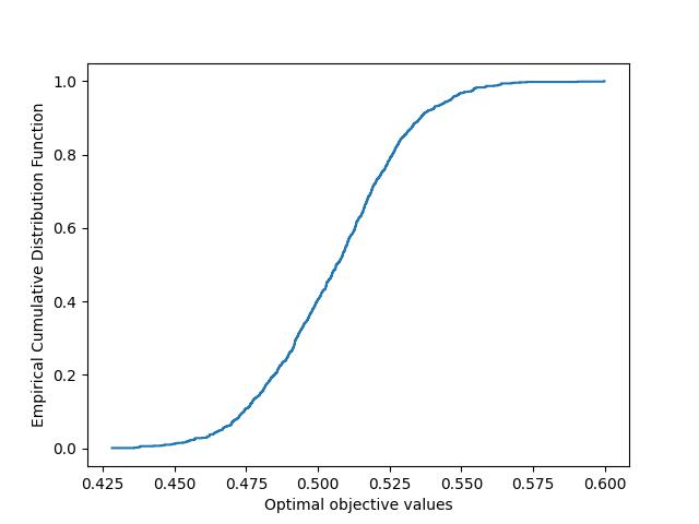
In our numerical experiments, we consider Gaussian and Rademacher random coefficient matrices of dimensions $m=1000$ and $n=50$. The sample size in either case is taken to be $1000$. As in the previous experiment, we take $c$ to be a random vector with i.i.d Rademacher components rescaled to have the Euclidean norm one. We generate the cost vector once so that it is the same for every LP from a sample. We employ the Kolmogorov–Smirnov (KS) test to compare the sample distribution of $z^{*}$ to Gaussian of a same mean and variance. In either case, the obtained p-value exceeds the conventional significance level of 0.05, indicating lack of substantial evidence to refute the null hypothesis that the data is normally distributed. Further, visual representation of the frequency histogram and the empirical cumulative distribution function of the optimal values shown in Figures 3 and 4 validate this conjecture.

The next conjecture summarizes the experimental findings:

Conjecture 6.1 (Limiting distribution of $z^{*}$).

Let $m$, $n$, $A(n)$ be as in Theorem 1.2, and for each $n$ let $c=c(n)$ be uniform random unit cost vector independent from $A(n)$. Then the sequence of normalized random variables

$$\frac{z^{*}-{\mathbb{E}}\,z^{*}}{\sqrt{{\rm Var}\,z^{*}}}$$

converges in distribution to the standard Gaussian.

6.4 Standard deviation of the optimal objective value

As in the previous two numerical experiments, in this one we consider two types of the entries distributions: Gaussian and Rademacher. The cost vector is generated according to the same procedure as above. We sample the LP (1) taking the sample size to be $50$, and compute the sample standard deviation $\hat{\sigma}$ (the square root of the sample variance) of the optimal objective value. Based on our numerical studies we speculate that standard deviation of $z^{*}$ is roughly of the order $1/\sqrt{m}$, at least in the setting where $m$ is very large compared to $n$. Indeed, upon examination of the last column in Tables 4 and 5, we observe a consistent phenomenon: the quantities are of order $1$ for various choices of $m$ and $n$.

$m$	$n$	$ab$	$\hat{\sigma}$	$\hat{\sigma}\times\sqrt{m}$
1000	50	0.408539	0.02420	0.765
2000	50	0.368161	0.01728	0.773
4000	50	0.337791	0.01333	0.843
6000	50	0.323170	0.01142	0.885
8000	50	0.313877	0.01059	0.947
10000	50	0.307196	0.01027	1.027
1000	100	0.465991	0.03014	0.953
2000	100	0.408539	0.01592	0.712
4000	100	0.368161	0.01172	0.742
6000	100	0.349456	0.00990	0.767
1000	150	0.528257	0.03192	1.010
2000	150	0.441515	0.015066	0.674
4000	150	0.391745	0.01155	0.731
6000	150	0.368161	0.011850	0.918

Table 4: Sample standard deviation of the optimal objective value with Gaussian matrix $A$ (the sample size = $50$)

$m$	$n$	$ab$	$\hat{\sigma}$	$\hat{\sigma}\times\sqrt{m}$
1000	50	0.408539	0.020420	0.645
2000	50	0.368161	0.017393	0.777
4000	50	0.337791	0.011962	0.756
6000	50	0.323170	0.010207	0.790
8000	50	0.313877	0.010333	0.924
10000	50	0.307196	0.008997	0.899
1000	100	0.465991	0.023097	0.730
2000	100	0.408539	0.014648	0.655
4000	100	0.368161	0.010436	0.660
6000	100	0.349456	0.011791	0.913
1000	150	0.528257	0.032600	1.030
2000	150	0.441515	0.015466	0.691
4000	150	0.391745	0.011030	0.697
6000	150	0.368161	0.009153	0.708

Table 5: The sample standard deviation of the optimal objective value with Rademacher matrix $A$ (the sample size = $50$)

6.5 An algorithm for finding a near-optimal feasible solution

As previously discussed, the proof of Theorem 3.1 involves an iterative projection process to restore feasibility from an initial point. In the process, we discretize the continuous space spanned by violated constraints at each iteration (i.e use a covering argument) as a means to apply probabilistic union bound. Recall that the goal of Algorithm 1 described in the proof of Theorem 3.1 is to provide theoretical guarantees for $z^{*}$. An exact software implementation of that algorithm is heavy in terms of both the amount of code and computations. On the other hand, it is of considerable interest to measure performance of block-iterative projection methods in the context of finding near optimal solution to instances of the random LP (1). To approach this task, we consider a “light” version of the algorithm from the proof of Theorem 3.1, which does not involve any discretizations (see Algorithm 2 below). The algorithm is a version of the classical Kaczmarz block-iterative projection method as presented in [18] and its randomized counterparts in [38] and [53]. In our context, the blocks correspond to the rows of the matrix $A$ that are violated by the initial point and its updates at each iteration. Table 6 shows the results of running the algorithm for various parameters $m$ and $n$. For each instance of the LP, $r$ is the the number of iterations required to restore feasibility, $x_{0}=(2\log(m/n))^{-\frac{1}{2}}c$ is the initial point and $x$ is the output of the Algorithm 2. Note that the obtained perturbations to $x_{0}$ are in the orthogonal complement of the cost vector $c$ and as a result $\|x_{0}\|_{2}=z(x)$. The numbers $|I_{0}|$ and $|I_{1}|$ are the number of violated constraints by $x_{0}$ at iteration 1 and $x_{0}+x_{1}$ at iteration 2, respectively. Note that these numbers are rather small compared to the size of the LP instance. We note that in our experiment, the algorithm did not converge for the $20000\times 50$ instance of the LP, which we attribute to the random nature of the problem. At the same time, the Algorithm converged fast due to small number of constraint violations for all other given instances.

Input: $A$: $m\times n$ standard Gaussian random matrix,

       $c$: random cost vector uniformly distributed on the sphere

Output: $x$: near-optimal feasible solution to LP (1)

1 $x\leftarrow(2\log(m/n))^{-\frac{1}{2}}c$;

2 $j\leftarrow 0$;

3 $\epsilon\leftarrow 0.1$;

4 while $x$ is not feasible do

5    $j\leftarrow j+1$;

6    Find the set of constraints $I_{j-1}$ that are violated or nearly violated by $x$, i.e all indices $i$ with $\langle{\rm row}_{i}(A),x\rangle>1-\epsilon$;

7    Compute vector $b$ where $b_{i}=1-\epsilon-\langle{\rm row}_{i}(A),x\rangle$ for all $i\in I_{j-1}$;

8    Project the constraints into the space $c^{\perp}$ (i.e define $v_{i}={\rm row}_{i}(A)-\langle{\rm row}_{i}(A),c\rangle c$ for all $i\in I_{j-1}$) ;

9    Find $x_{j}$ as a linear combination of $v_{i}$’s, $i\in I_{j-1}$, so that the constraints violated by $x$ are repaired (specifically, solve the linear system $M^{T}Mu=b$ for $u$, then solve $x_{j}=Mu$ where $M$ is the matrix with columns $v_{i}$);

10    $\epsilon\leftarrow\epsilon*0.1$;

11    $x\leftarrow x+x_{j}$;

12   

13 end while

14return $x$

Algorithm 2 Algorithm for finding near-optimal feasible solution to LP (1), an instance of block-iterative Kaczmarz projection method

$m$	$n$	$r$	$\|x_{0}\|_{2}=z(x)$	$|I_{0}|$	$|I_{1}|$
1000	50	2	0.408539	11	1
1000	100	2	0.465991	28	4
2000	50	2	0.368161	6	1
2000	100	2	0.408539	23	1
4000	50	2	0.337791	13	2
4000	100	2	0.368161	30	1
6000	50	2	0.323170	22	21
6000	100	2	0.349456	31	8
8000	50	2	0.313877	22	6
8000	100	2	0.337791	21	5
10000	50	2	0.307196	19	1
10000	100	1	0.329505	34	0
20000	100	1	0.307196	29	0
40000	50	1	0.273493	12	0
40000	100	2	0.288881	34	3
60000	50	2	0.265558	16	2
60000	100	1	0.279576	36	0
80000	50	1	0.260329	21	0
80000	100	2	0.273493	36	1
100000	50	2	0.256479	28	5
100000	100	2	0.269040	35	1

Table 6: Numerical results for the Algorithm 2 for various $m$ and $n$ ($r$ = the number of iterations to restore the feasibility).

7 Conclusion

In this paper, we study the optimal objective value $z^{*}$ of a random linear program where the entries of the $m\times n$ coefficient matrix $A$ have subgaussian distributions, the variables $x_{1},\dots,x_{n}$ are free and the right hand side of each constraint is $1$. We establish sharp asymptotics $z^{*}=(1\pm o(1))(2\log(m/n))^{-\frac{1}{2}}$ in the regime $n\to\infty$, $\frac{m}{n}\to\infty$ and some additional assumptions on the cost vectors. This asymptotic provides quantitative information about the geometry of the random polyhedron defined by the feasible region of the random LP (1), specifically about its spherical mean width. The computational experiments support our theoretical guarantees and give insights into several open questions regarding the asymptotic behaviour of the random LP. The connection between the proof of the main result and convex feasibility problems allows us to provide a fast algorithm for obtaining a near optimal solution in our randomized setting. The random LP (1) is a step towards studying models with inhomogeneous coefficient matrices and establishing stronger connections to practical applications.

Declarations

Funding. Konstantin Tikhomirov is partially supported by the NSF grant DMS-2331037.

Conflict of interest/Competing interests. The authors declare no conflict of interest in regard to this publication.

Code availability. The code for the numerical experiments is available on https://github.com/marzb93/RandomLinearProgram

References

- [1] (1954) The relaxation method for linear inequalities. Canad. J. Math. 6, pp. 382–392. External Links: ISSN 0008-414X, Document, Link, MathReview (L. M. Blumenthal) Cited by: §1.4.1.
- [2] (1989) Block-iterative projection methods for parallel computation of solutions to convex feasibility problems. Linear Algebra and Its Applications 120, pp. 165–175. Cited by: §1.4.1.
- [3] (2015) On the Gaussian behavior of marginals and the mean width of random polytopes. Proc. Amer. Math. Soc. 143 (2), pp. 821–832. External Links: ISSN 0002-9939, Document, Link, MathReview (Gergely Ambrus) Cited by: §1.4.3.
- [4] (1955) Distributions of solutions of a set of linear equations (with an application to linear programming). Journal of the American Statistical Association 50 (271), pp. 854–869. Cited by: 3rd item.
- [5] (2018) On greedy randomized Kaczmarz method for solving large sparse linear systems. SIAM J. Sci. Comput. 40 (1), pp. A592–A606. External Links: ISSN 1064-8275, Document, Link, MathReview (Stefan A. Funken) Cited by: §1.4.1.
- [6] (1986) Random linear programs with many variables and few constraints. Math. Programming 34 (1), pp. 62–71. External Links: ISSN 0025-5610, Document, Link, MathReview (H. L. Bhatia) Cited by: 1st item.
- [7] (1982) The average number of pivot steps required by the simplex-method is polynomial. Z. Oper. Res. Ser. A-B 26 (5), pp. A157–A177. External Links: ISSN 0340-9422, Document, Link, MathReview (C. A. Botsaris) Cited by: item (i), 1st item.
- [8] (1999) A sharp upper bound for the expected number of shadow vertices in LP-polyhedra under orthogonal projection on two-dimensional planes. Math. Oper. Res. 24 (3), pp. 544–603. External Links: ISSN 0364-765X, Document, Link, MathReview (K. G. Murty) Cited by: item (i), 1st item.
- [9] (1987) The simplex method. Algorithms and Combinatorics: Study and Research Texts, Vol. 1, Springer-Verlag, Berlin. Note: A probabilistic analysis External Links: ISBN 3-540-17096-0, Document, Link, MathReview (Jürgen Köhler) Cited by: item (i), 1st item.
- [10] (2014) Integer feasibility of random polytopes: random integer programs. In Proceedings of the 5th conference on Innovations in theoretical computer science, pp. 449–458. Cited by: 4th item.
- [11] (2015) A polynomial projection algorithm for linear feasibility problems. Math. Program. 153 (2, Ser. A), pp. 687–713. External Links: ISSN 0025-5610, Document, Link, MathReview (Wei Hong Yang) Cited by: §1.4.1.
- [12] (2018) A friendly smoothed analysis of the simplex method. In STOC’18—Proceedings of the 50th Annual ACM SIGACT Symposium on Theory of Computing, pp. 390–403. External Links: Document, Link, MathReview Entry Cited by: 2nd item.
- [13] (2009) Asymptotic shape of a random polytope in a convex body. J. Funct. Anal. 257 (9), pp. 2820–2839. External Links: ISSN 0022-1236, Document, Link, MathReview (J. Hüsler) Cited by: §1.4.3.
- [14] (2017) A sampling Kaczmarz-Motzkin algorithm for linear feasibility. SIAM J. Sci. Comput. 39 (5), pp. S66–S87. External Links: ISSN 1064-8275, Document, Link, MathReview (Emanuele Galligani) Cited by: §1.4.1.
- [15] (1998) Large deviations techniques and applications. Second edition, Applications of Mathematics (New York), Vol. 38, Springer-Verlag, New York. External Links: ISBN 0-387-98406-2, Document, Link, MathReview Entry Cited by: §2.3, Acknowledgements.
- [16] (1986) On linear programs with random costs. Mathematical Programming 35, pp. 3–16. Cited by: 5th item.
- [17] (2011) Acceleration of randomized Kaczmarz method via the Johnson-Lindenstrauss lemma. Numer. Algorithms 58 (2), pp. 163–177. External Links: ISSN 1017-1398, Document, Link, MathReview (Alexander N. Malyshev) Cited by: §1.4.1.
- [18] (1980) Block-iterative methods for consistent and inconsistent linear equations. Numerische Mathematik 35, pp. 1–12. Cited by: §6.5.
- [19] (1991) An introduction to probability theory and its applications, volume 2. Vol. 81, John Wiley & Sons. Cited by: §5.1.
- [20] (2002) Random spaces generated by vertices of the cube. Discrete Comput. Geom. 28 (2), pp. 255–273. External Links: ISSN 0179-5376, Document, Link, MathReview (Z. Nádeník) Cited by: §1.4.3.
- [21] (2016) Asymptotic shape of the convex hull of isotropic log-concave random vectors. Adv. in Appl. Math. 75, pp. 116–143. External Links: ISSN 0196-8858, Document, Link, MathReview (Julio Bernués) Cited by: §1.4.3.
- [22] (1986) An octahedron is poorly approximated by random subspaces. Funktsional. Anal. i Prilozhen. 20 (1), pp. 14–20, 96. External Links: ISSN 0374-1990, MathReview (M. I. Kadets) Cited by: §1.4.3.
- [23] (1988) Extremal properties of orthogonal parallelepipeds and their applications to the geometry of Banach spaces. Mat. Sb. (N.S.) 136(178) (1), pp. 85–96. External Links: ISSN 0368-8666, Document, Link, MathReview (G. M. Ustinov) Cited by: §1.4.3.
- [24] (2021) On adaptive sketch-and-project for solving linear systems. SIAM J. Matrix Anal. Appl. 42 (2), pp. 954–989. External Links: ISSN 0895-4798, Document, Link, MathReview Entry Cited by: §1.4.1.
- [25] (2015) Randomized iterative methods for linear systems. SIAM J. Matrix Anal. Appl. 36 (4), pp. 1660–1690. External Links: ISSN 0895-4798, Document, Link, MathReview (Ninoslav Truhar) Cited by: §1.4.1.
- [26] ([2023] ©2023) Upper and lower bounds on the smoothed complexity of the simplex method. In STOC’23—Proceedings of the 55th Annual ACM Symposium on Theory of Computing, pp. 1904–1917. External Links: Document, Link, MathReview Entry Cited by: 2nd item.
- [27] (2017) Preasymptotic convergence of randomized Kaczmarz method. Inverse Problems 33 (12), pp. 125012, 21. External Links: ISSN 0266-5611, Document, Link, MathReview (Barbara Zubik-Kowal) Cited by: §1.4.1.
- [28] (1937) Angenäherte auflösung von systemen linearer gleichungen (english translation by jason stockmann): bulletin international de l’académie polonaise des sciences et des lettres. Cited by: §1.4.1.
- [29] (2022) Limit laws for empirical optimal solutions in random linear programs. Annals of Operations Research 315 (1), pp. 251–278. Cited by: 3rd item.
- [30] (2005) Smallest singular value of random matrices and geometry of random polytopes. Adv. Math. 195 (2), pp. 491–523. External Links: ISSN 0001-8708, Document, Link, MathReview (Béla Uhrin) Cited by: §1.4.3, §1.4.3.
- [31] (2016) An accelerated randomized Kaczmarz algorithm. Math. Comp. 85 (297), pp. 153–178. External Links: ISSN 0025-5718, Document, Link, MathReview (Judith M. Ford) Cited by: §1.4.1.
- [32] (2023) Asymptotic confidence sets for random linear programs. arXiv preprint arXiv:2302.12364. Cited by: 3rd item.
- [33] (2021) On greedy randomized block Kaczmarz method for consistent linear systems. Linear Algebra Appl. 616, pp. 178–200. External Links: ISSN 0024-3795, Document, Link, MathReview (Bruno Carpentieri) Cited by: §1.4.1.
- [34] (2015) Convergence properties of the randomized extended Gauss-Seidel and Kaczmarz methods. SIAM J. Matrix Anal. Appl. 36 (4), pp. 1590–1604. External Links: ISSN 0895-4798, Document, Link, MathReview (Marco Donatelli) Cited by: §1.4.1.
- [35] (2020) Accelerated sampling Kaczmarz Motzkin algorithm for the linear feasibility problem. J. Global Optim. 77 (2), pp. 361–382. External Links: ISSN 0925-5001, Document, Link, MathReview (S. A. Edalatpanah) Cited by: §1.4.1.
- [36] (2022) Sampling kaczmarz-motzkin method for linear feasibility problems: generalization and acceleration. Mathematical Programming 194 (1-2), pp. 719–779. Cited by: §1.4.1.
- [37] (1954) The relaxation method for linear inequalities. Canadian Journal of Mathematics 6, pp. 393–404. Cited by: §1.4.1.
- [38] (2014) Paved with good intentions: analysis of a randomized block Kaczmarz method. Linear Algebra Appl. 441, pp. 199–221. External Links: ISSN 0024-3795, Document, Link, MathReview (A. Bultheel) Cited by: §1.4.1, §6.5.
- [39] (2020) A greedy block Kaczmarz algorithm for solving large-scale linear systems. Appl. Math. Lett. 104, pp. 106294, 8. External Links: ISSN 0893-9659, Document, Link, MathReview Entry Cited by: §1.4.1.
- [40] (1989) The volume of convex bodies and Banach space geometry. Cambridge Tracts in Mathematics, Vol. 94, Cambridge University Press, Cambridge. External Links: ISBN 0-521-36465-5; 0-521-66635-X, Document, Link, MathReview (Mikhail Ostrovskii) Cited by: item (ii).
- [41] (1966) On the probability distribution of the optimum of a random linear program. SIAM Journal on Control 4 (1), pp. 211–222. Cited by: 3rd item.
- [42] (2008) The Littlewood-Offord problem and invertibility of random matrices. Adv. Math. 218 (2), pp. 600–633. External Links: ISSN 0001-8708, Document, Link, MathReview (Ben Joseph Green) Cited by: Definition 2.2.
- [43] (1983) On the average number of steps of the simplex method of linear programming. Math. Programming 27 (3), pp. 241–262. External Links: ISSN 0025-5610, Document, Link, MathReview (M. Brannigan) Cited by: 1st item.
- [44] (2004) Smoothed analysis of algorithms: why the simplex algorithm usually takes polynomial time. J. ACM 51 (3), pp. 385–463. External Links: ISSN 0004-5411, Document, Link, MathReview (Panos M. Pardalos) Cited by: item (i), 2nd item.
- [45] (2009) A randomized Kaczmarz algorithm with exponential convergence. J. Fourier Anal. Appl. 15 (2), pp. 262–278. External Links: ISSN 1069-5869, Document, Link, MathReview (Xiaoping A. Shen) Cited by: §1.4.1.
- [46] (2011) Mean field models for spin glasses. Volume I. Ergebnisse der Mathematik und ihrer Grenzgebiete. 3. Folge. A Series of Modern Surveys in Mathematics [Results in Mathematics and Related Areas. 3rd Series. A Series of Modern Surveys in Mathematics], Vol. 54, Springer-Verlag, Berlin. Note: Basic examples External Links: ISBN 978-3-642-15201-6, Document, Link, MathReview (Francis Comets) Cited by: §1.4.1.
- [47] (2011) Mean field models for spin glasses. Volume II. Ergebnisse der Mathematik und ihrer Grenzgebiete. 3. Folge. A Series of Modern Surveys in Mathematics [Results in Mathematics and Related Areas. 3rd Series. A Series of Modern Surveys in Mathematics], Vol. 55, Springer, Heidelberg. Note: Advanced replica-symmetry and low temperature External Links: ISBN 978-3-642-22252-8; 978-3-642-22253-5, MathReview (Francis Comets) Cited by: §1.4.1.
- [48] (1982) On relaxation methods for systems of linear inequalities. European J. Oper. Res. 9 (2), pp. 184–189. External Links: ISSN 0377-2217, Document, Link, MathReview Entry Cited by: §1.4.1.
- [49] (2009) Beyond Hirsch conjecture: walks on random polytopes and smoothed complexity of the simplex method. SIAM J. Comput. 39 (2), pp. 646–678. External Links: ISSN 0097-5397, Document, Link, MathReview Entry Cited by: 2nd item.
- [50] (2018) High-dimensional probability. Cambridge Series in Statistical and Probabilistic Mathematics, Vol. 47, Cambridge University Press, Cambridge. Note: An introduction with applications in data science, With a foreword by Sara van de Geer External Links: ISBN 978-1-108-41519-4, Document, Link, MathReview (Sasha Sodin) Cited by: item (ii), §1.2, §2.2, §2.3, §3.1, §3.1, §3.1, §3.1, §3.3, §4.1, §4.1, §4.2, §4.2, §5.1, §5.1.
- [51] (2021) Block sampling kaczmarz–motzkin methods for consistent linear systems. Calcolo 58 (3), pp. 39. Cited by: §1.4.1.
- [52] (2022) Greedy Motzkin-Kaczmarz methods for solving linear systems. Numer. Linear Algebra Appl. 29 (4), pp. Paper No. e2429, 24. External Links: ISSN 1070-5325, MathReview Entry Cited by: §1.4.1.
- [53] (2023) Randomized block subsampling Kaczmarz-Motzkin method. Linear Algebra Appl. 667, pp. 133–150. External Links: ISSN 0024-3795, Document, Link, MathReview Entry Cited by: §1.4.1, §6.5.