arXiv is now an independent nonprofit! Learn more
License: arXiv.org perpetual non-exclusive license
arXiv:2401.15021v2 [math.PR] 27 Aug 2025

Volterra equations with affine drift: looking for stationarity. Application to the quadratic rough Heston model

Gilles Pagès ††thanks: Sorbonne Université, Laboratoire de Probabilités, Statistique et Modélisation, case 158, 4, pl. Jussieu, F-75252 Paris Cedex 5, France. E-mail: gilles.pages@sorbonne-universite.fr††thanks: This research benefited from the support of the “Chaire Risques Financiers”, Fondation du Risque.
Abstract

We investigate the properties of the solutions of scaled Volterra equations (i.e. with an affine mean-reverting drift) in terms of stationarity at both a finite horizon and on the long run. In particular we prove that such an equation never has a stationary regime, except if the kernel is constant (i.e. the equation is a standard Brownian diffusion) or in some fully degenerate pathological settings. We introduce a deterministic stabilizer ς\varsigma associated to the kernel which may produce a fake stationary regime in the sense that all the marginals share the same expectation and variance. We also show that the marginals of such a process when starting various initial values are confluent in L2L^{2} as time goes to infinity. We establish that for some classes of diffusion coefficients (square root of positive quadratic polynomials) the time shifted solutions of such Volterra equations weakly functionally converge toward a family of L2L^{2}-stationary processes sharing the same covariance function. We apply these results to a family of stabilized quadratic rough volatility models (when the kernel K⁡(t)=tH−12Γ⁡(H+12)K(t)=\frac{t^{H-\frac{1}{2}}}{\Gamma(H+\frac{1}{2})}, 0<H<120<H<\frac{1}{2}) which produces examples Volterra processes sharing a fake stationary regime.

Introduction

We investigate in this paper conditions under which stochastic Volterra equations with affine drifts and convolutive kernels of the form

Xt=X0+∫0tK⁡(t−s)​(μ⁡(s)−λ​Xs)​𝑑s+∫0tK⁡(t−s)​σ​(Xs)​d​WsX_{t}=X_{0}+\int_{0}^{t}K(t-s)(\mu(s)-\lambda X_{s})ds+\int_{0}^{t}K(t-s)\sigma(X_{s})dW_{s}

have a stationarity regime in the classical sense, i.e. the distribution of the process is invariant by time shift (see [15]) or in a weaker sense – that we called fake stationary regime (of type I) – in which the solution only has constant mean and variance at every instant tt. In the Gaussian case (typically pseudo-Ornstein-Uhlenbeck process), it implies that the process has the same 11-marginal distribution at very time tt (which could be called a fake stationary regime of type II). However such a property if it holds does not imply stationarity nor classical weak L2L^{2}-stationarity (based on covariance).

In terms of application this may have consequences on rough volatility models (see [2, 8, 11, 12]) which met a great success in the financial community during these last ten years, in particular because it provides a consistent modeling of the dynamics of financial markets (mostly equity) at various scales from the order book to the pricing of derivative products in spite of its non-Markovian feature. In the original version of these rough stochastic volatility models, mostly derived from the regular Heston model, the mean-reverting CIR dynamics of the volatility is replaced by a Volterra version of this CIR process in which the convolution kernel is singular and of fractional form K⁡(t)=tH−12K(t)=t^{H-\frac{1}{2}} for some H∈(0,1/2)H\!\in(0,1/2) (Hurst coefficients). In the late 1990’s, attempts to model the long memory effect on continuous time stochastic volatility models (see [6, 7]) also relied on similar stochastic Volterra equations using the same family of kernels but with H∈(1/2,1)H\!\in(1/2,1). In both cases the aim is to mimic the behaviour of a stochastic differential equations (SDE) driven by a fractional Brownian motion without having to face the technicalities of such equations which rely on rough path theory, technicalities which can become extreme when HH gets close to 00.

If we come back for a while to the standard Heston model equipped with its CIR driven stochastic volatility process, it has been observed for long by practitioners that this model was difficult to calibrate (on vanilla products) to produce good prices for derivatives with short maturities, especially path-dependent ones. This is most likely due to the fact that the CIR process is usually initialized by a deterministic value at the origin (often the long run mean). So this volatility dynamics actually has two regimes, first, one for short maturities when the starting value is prominent and the variance is very small, then it deploys until attaining its its stationary regime – a γ\gamma-distribution –. A solution to get rid of this drawback is to consider directly a Heston model in which the volatility is taken under its stationary regime (see e.g. [21]) which also has the advantage to reduce by one the number of parameters. A quantization based approach is provided for calibration and pricing of path-dependent derivatives (at least under the Feller condition that ensures positivity of the volatility) in a recent paper [18].

If, as it is likely, a similar problem occurs for rough volatility models based on the rough Volterra version of the CIR model, the search for some stationarity properties of such a rough CIR model can be of interest to make possible a calibration consistent for both short and long maturities. This does not provide a plug-and-play solution to this problem but explores in an elementary way what are or could be the connexions between stationarity and Volterra equations with “mean-reverting” affine drift with a mitigate conclusion. This could be compared to the recent paper [15] about ergodicity of Volterra processes.

The paper is organized as follows. In Section 1 we recall the main properties of stochastic Volterra equations with convolutive drifts: existence, moment control, etc, with a focus on those of these processes having an affine drift. In that case some specific tools are available like the Resolvent and the solution Wiener-Hopf equation which corresponds when K⁡(t)=eλ​tK(t)=e^{\lambda t} (Markovian framework) to apply Itô’s lemma to eλ​t​Xte^{\lambda t}X_{t}. In Section 2 we elucidate when a Volterra equation with affine has an invariant distribution (distribution invariant by time shift). We show that this situation is essentially degenerate in the sense that it implies that the kernel KK is constant i.e. that the Volterra equation is a standard Brownian equation. In Section 3 we define some notions of fake stationarity like having constant mean and variance (type I), or constant 11-marginal distribution (type II). To this end we are led to introduce a multiplicative deterministic functionς\varsigma in the Brownian convolution, called stabilizer to “control” the process (through its volatility coefficient). This stabilizer is solution to an intrinsic convolution equation related to the kernel of the equation. In Section 3.2.2 we provide examples of such“fake stationary” stabilized processes with some explicit computations when

σ⁡(x)=κ0+κ1​(x−μ0λ)+κ2​(x−μ0λ)2 with κi≥0,i=1,2,κ12≤4​κ0​κ2.\sigma(x)=\sqrt{\kappa_{0}+\kappa_{1}\,(x-\tfrac{\mu_{0}}{\lambda})+\kappa_{2}\,(x-\tfrac{\mu_{0}}{\lambda})^{2}}\quad\mbox{ with }\quad\kappa_{i}\geq 0,\;i=1,2,\;\kappa^{2}_{1}\leq 4\kappa_{0}\kappa_{2}.

This form of the diffusion coefficient appears e.g. in [12] when modeling the volatility in the quadratic rough Heston model. We also investigate for such stabilized processes the functional weak asymptotics of the time shifted process (Xt+s)s≥0(X_{t+s})_{s\geq 0} as t→+∞t\to+\infty which turns out to be a weak L2L^{2}-stationary process. Finally in Section 5 we apply our results to the case case of fractional kernels Kα​(t)=tα−1K_{\alpha}(t)=t^{\alpha-1}, α∈(0,1)\alpha\,\in(0,1) covering “rough” models (where α=12+H\alpha=\frac{1}{2}+H, H∈(0,1/2)H\!\in(0,1/2), the Hurst coefficient). In particular we prove the existence of the stabilizer with a semi-closed form as (fractional) power series whose coefficients can be computed by induction. We prove in an appendix that this series has an infinite convergence radius, null at 00, increasing toward a finite (identified) limit at infinity.

Notations. ∙\bullet Leb1{\rm Leb}_{1} (resp. Lebℝ+{\rm Leb}_{{\mathbb{R}}_{+}}) denotes the Lebesgue measure on ℝ{\mathbb{R}} (resp. ℝ+=[0,+∞){\mathbb{R}}_{+}=[0,+\infty)).

∙\bullet For f,g∈ℒℝ+,l​o​c1​(ℝ+,Leb1)f,g\!\in{\cal L}_{{\mathbb{R}}_{+},loc}^{1}({\mathbb{R}}_{+},{\rm Leb}_{1}), we define their convolution by f∗g⁡(t)=∫0tf⁡(t−s)​g​(s)​𝑑sf*g(t)=\int_{0}^{t}f(t-s)g(s)ds, t≥0t\geq 0.

∙\bullet For f,g∈ℒℝ+,l​o​c2​(ℝ+,Leb1)f,g\!\in{\cal L}_{{\mathbb{R}}_{+},loc}^{2}({\mathbb{R}}_{+},{\rm Leb}_{1}) and WW a Brownian motion, we define their stochastic convolution by

f∗Wg=∫0tf⁡(t−s)​g​(s)​d​Ws,t≥0.f\stackrel{{\scriptstyle W}}{{*}}g=\int_{0}^{t}f(t-s)g(s)dW_{s},\quad t\geq 0.

∙\bullet [X][X] stands for the distribution of the random variable/vector/process XX.

∙\bullet X⟂⟂YX\perp\!\!\!\perp Y stands for the independence of the two random objects XX and YY.

1 Background on Volterra SDEs with convolutive kernels

1.1 Volterra processes with convolutive kernels

We are interested in the stochastic Volterra equation

Xt=X0+∫0tK⁡(t−s)​b​(s,Xs)​𝑑s+∫0tK⁡(t−s)​σ​(s,Xs)​d​Ws,t≥0,X_{t}=X_{0}+\int_{0}^{t}K(t-s)b(s,X_{s})ds+\int_{0}^{t}K(t-s)\sigma(s,X_{s})dW_{s},\quad t\geq 0, (1.1)

where b:[0,T]×ℝ→ℝb:[0,T]\times{\mathbb{R}}\to{\mathbb{R}}, σ:[0,T]×ℝ→ℝ\sigma:[0,T]\times{\mathbb{R}}\to{\mathbb{R}} are Borel measurable, K∈ℒl​o​c,ℝ+2​(Leb1)K\!\in{\cal L}^{2}_{loc,{\mathbb{R}}_{+}}({\rm Leb}_{1}) is a convolutive kernel and (Wt)t≥0(W_{t})_{t\geq 0} is a standard Brownian motion independent from the ℝ{\mathbb{R}}-valued random variable X0X_{0} both defined on a probability space (Ω,𝒜,ℙ)(\Omega,{\cal A},{\mathbb{P}}). Let (ℱt)t≥0({\cal F}_{t})_{t\geq 0} be a filtration (satisfying the usual conditions) such that X0X_{0} is ℱ0{\cal F}_{0}-measurable and WW is an (ℱt)({\cal F}_{t})-Brownian motion independent of X0X_{0}.

Assume that the kernel KK satisfies

∃β>1such thatK∈Ll​o​c2​β​(Leb1)\exists\,\beta>1\quad\mbox{such that}\quad K\!\in L^{2\beta}_{loc}({\rm Leb}_{1}) (1.2)

and that, for every T>0T>0,

(𝒦T,θc​o​n​t)∃κT<+∞,∃θT>0,∀δ∈(0,T),supt∈[0,T][∫0t|K((s+δ)∧T)−K(s))|2ds]12≤κTδθT.({\cal K}^{cont}_{T,\theta})\;\exists\,\kappa_{{}_{T}}<+\infty,\;\exists\,\theta_{{}_{T}}>0,\;\forall\,\delta\!\in(0,T),\;\sup_{t\in[0,T]}\left[\int_{0}^{t}|K(\big(s+\delta)\wedge T\big)-K(s))|^{2}ds\right]^{\frac{1}{2}}\leq\kappa_{{}_{T}}\,\delta^{\theta_{{}_{T}}}. (1.3)

Assume bb and σ\sigma satisfy the following Lipschitz-linear growth assumption uniform in time

(i)\displaystyle(i) ∀t∈[0,T],∀x,y∈ℝ,|b⁡(t,x)−b⁡(t,y)+|​σ​(t,x)−σ⁡(t,y)|≤Cb,σ,T​|x−y|,\displaystyle\;\forall\,t\!\in[0,T],\;\forall\,x,\,y\!\in{\mathbb{R}},\;|b(t,x)-b(t,y)+|\sigma(t,x)-\sigma(t,y)|\leq C_{b,\sigma,T}|x-y|,
(i​i)\displaystyle(ii) supt∈[0,T]|b⁡(t,0)|+|σ⁡(t,0)|<+∞.\displaystyle\sup_{t\in[0,T]}|b(t,0)|+|\sigma(t,0)|<+\infty.

It has been established in [17, Theorem 1.1] that, if X0∈Lp​(ℙ)X_{0}\!\in L^{p}({\mathbb{P}}) for some p>0p>0, then Equation (1.1) admits a unique pathwise continuous solution on ℝ+{\mathbb{R}}_{+} starting from X0X_{0} satisfying (among other properties),

∀T>0,∃Cp,T>0,∥supt∈[0,T]|Xt|∥p≤Cp,T(1+∥X0∥p).\forall\,T>0,\;\exists\,C_{{}_{p,T}}>0,\quad\Big\|\sup_{t\in[0,T]}|X_{t}|\Big\|_{p}\leq C_{{}_{p,T}}(1+\|X_{0}\|_{p}). (1.4)

This result appears as a generalization of the classical strong existence-uniqueness result of pathwise continuous solutions established in [25], only when the starting value X0X_{0} has finite polynomial moments at any order (The framework is more general).

1.2 Laplace Transform

Let us first introduce the Laplace transform of a Borel function f:ℝ+→ℝ+f:{\mathbb{R}}_{+}\to{\mathbb{R}}_{+} by

∀t≥0,Lf​(t)=∫0+∞e−t​u​f​(u)​𝑑u∈[0,∞].\forall\,t\geq 0,\quad L_{f}(t)=\int_{0}^{+\infty}e^{-tu}f(u)du\!\in[0,\infty].

This Laplace transform is non-increasing and if Lf​(t0)<+∞L_{f}(t_{0})<+\infty for some t0≥0t_{0}\geq 0, then Lf​(t)→0L_{f}(t)\to 0 as t→+∞t\to+\infty.

One can define the Laplace transform of a Borel function f:ℝ+→ℝf:{\mathbb{R}}_{+}\to{\mathbb{R}} on (0,+∞)(0,+\infty) as soon as L|f|​(t)<+∞L_{|f|}(t)<+\infty for every t>0t>0 by the above formula. The Laplace transform can be extended to ℝ+{\mathbb{R}}_{+} as an ℝ{\mathbb{R}}-valued function if f∈ℒℝ+1​(Leb1)f\!\in{\cal L}^{1}_{{\mathbb{R}}_{+}}({\rm Leb}_{1}).

1.3 Resolvent of a convolutive kernel

For every λ∈ℝ\lambda\!\in{\mathbb{R}}, the resolvent RλR_{\lambda} associated to KK and λ\lambda is defined as the unique solution – if it exists – to the deterministic Volterra equation

∀t≥0,Rλ​(t)+λ​∫0tK⁡(t−s)​Rλ​(s)​𝑑s=1\forall\,t\geq 0,\quad R_{\lambda}(t)+\lambda\int_{0}^{t}K(t-s)R_{\lambda}(s)ds=1 (1.5)

or, equivalently, written in terms of convolution,

Rλ+λ​K∗Rλ=1.R_{\lambda}+\lambda K*R_{\lambda}=1. (1.6)

The solution always satisfies Rλ​(0)=1R_{\lambda}(0)=1 and formally reads

Rλ=∑k≥0(−1)k​λk​(1∗K∗k)R_{\lambda}=\sum_{k\geq 0}(-1)^{k}\lambda^{k}(\mbox{\bf 1}*K^{*k}) (1.7)

where, by convention in this formula, K∗0=δ0K^{*0}=\delta_{0} (Dirac mass at 00).

From now on we will assume that the kernel KK satisfies

(ℒK)∀t>0,LK​(t)<+∞.({\cal L}_{K})\qquad\forall\,t>0,\quad L_{K}(t)<+\infty. (1.8)

∙\bullet If λ>0\lambda>0, (1.7) defines an absolutely convergent series for every t∈(tK,+∞)t\!\in(t_{K},+\infty) where tK=inf{t:LK​(t)≤1/λ}<+∞t_{K}=\inf\{t:L_{K}(t)\leq 1/\lambda\}<+\infty.

∙\bullet If the (non-negative) kernel KK satisfies

0≤K⁡(t)≤C​eb​t​ta−1​ for some ​a,b,C>∈ℝ+0\leq K(t)\leq Ce^{bt}t^{a-1}\mbox{ for some }\;a,\,\;b,\;C>0\!\in{\mathbb{R}}_{+} (1.9)

then one easily checks by induction that

1∗K∗n​(t)≤Cn​eb​t​Γ​(a)nΓ⁡(a​n+1)​ta​n,\mbox{\bf 1}*K^{*n}(t)\leq C^{n}e^{bt}\frac{\Gamma(a)^{n}}{\Gamma(an+1)}t^{an}, (1.10)

where Γ⁡(a)=∫0+∞e−u​ua−1​𝑑u\Gamma(a)=\int_{0}^{+\infty}e^{-u}u^{a-1}du. Then, one shows using Stirling formula that, for such kernels, the above series (1.7) is absolutely converging for every t>0t>0 so that the function RλR_{\lambda} is well-defined on (0,+∞)(0,+\infty).

∙\bullet If KK is regular enough (say continuous) the resolvent RλR_{\lambda} is differentiable and one checks that fλ=−Rλ′f_{\lambda}=-R^{\prime}_{\lambda} satisfies, for every t>0t>0,

−fλ​(t)+λ⁡(Rλ​(0)​K​(t)−K∗fλ​(t))=0-f_{\lambda}(t)+\lambda\big(R_{\lambda}(0)K(t)-K*f_{\lambda}(t)\big)=0

that is fλf_{\lambda} is solution to the equation

fλ+λ​K∗fλ=λ​K.f_{\lambda}+\lambda K*f_{\lambda}=\lambda K. (1.11)

In particular, if RλR_{\lambda} turns out to be non-increasing, then fλf_{\lambda} is non-negative and satisfies 0≤fλ≤λ​K0\leq f_{\lambda}\leq\lambda K. In that case one also has that ∫0+∞fλ​(t)​𝑑t=1−Rλ​(+∞)\int_{0}^{+\infty}f_{\lambda}(t)dt=1-R_{\lambda}(+\infty), so that fλf_{\lambda} is a probability density if and only if limt→+∞Rλ​(t)=0\displaystyle\lim_{t\to+\infty}R_{\lambda}(t)=0.

Examples of kernels.

  1. 1.

    Trivial kernel (Markov). Let K​(t)=1ℝ+​(t)K(t)=\mbox{\bf 1}_{{\mathbb{R}}_{+}}(t). It obviously satisfies (1.2), (1.3) and (1.9). Then Rλ​(t)=e−λ​tR_{\lambda}(t)=e^{-\lambda t}.

  2. 2.

    Exponential kernel. Let K⁡(t)=e−uK(t)=e^{-u}. It clearly satisfies (1.2), (1.3) and (1.9). Then Rλ​(t)={t+1if ​λ=−11+λ​e−(λ+1)​tλ+1if ​λ≠−1R_{\lambda}(t)=\left\{\begin{array}[]{cc}t+1&\mbox{if }\lambda=-1\\ \frac{1+\lambda e^{-(\lambda+1)t}}{\lambda+1}&\mbox{if }\lambda\neq-1\end{array}\right..

  3. 3.

    Fractional integration kernel. Let

    K⁡(t)=Kα​(t)=uα−1Γ⁡(α)​1ℝ+​(t),α>0.K(t)=K_{\alpha}(t)=\frac{u^{\alpha-1}}{\Gamma(\alpha)}\mbox{\bf 1}_{{\mathbb{R}}_{+}}(t),\quad\alpha>0. (1.12)

    These kernels satisfy (1.2) and (1.3) for α>1/2\alpha>1/2 (with θT=(α−12)∧1\theta_{{}_{T}}=(\alpha-\frac{1}{2})\wedge 1, see [24] or [17] along many others) among many others and trivially (1.9). This family of kernels corresponds to the fractional integrations of order α>0\alpha>0.

    It follows from the easy identity Kα∗Kα′=Kα+α′K_{\alpha}*K_{\alpha^{\prime}}=K_{\alpha+\alpha^{\prime}} that

    Rα,λ​(t)=∑k≥0(−1)k​λk​tα​kΓ⁡(α​k+1)=Eα​(−λ​tα)​t≥0,R_{\alpha,\lambda}(t)=\sum_{k\geq 0}(-1)^{k}\frac{\lambda^{k}t^{\alpha k}}{\Gamma(\alpha k+1)}=E_{\alpha}(-\lambda t^{\alpha})\;t\geq 0, (1.13)

    where EαE_{\alpha} denotes the standard Mittag-Leffler function

    Eα​(t)=∑k≥0tkΓ⁡(α​k+1),t∈ℝ.E_{\alpha}(t)=\sum_{k\geq 0}\frac{t^{k}}{\Gamma(\alpha k+1)},\ t\!\in{\mathbb{R}}.

    One shows (see [13] and Section 5 further on) that EαE_{\alpha} is increasing and differentiable on the real line with limt→+∞Eα​(t)=+∞\displaystyle\lim_{t\to+\infty}E_{\alpha}(t)=+\infty and Eα​(0)=1E_{\alpha}(0)=1. In particular, EαE_{\alpha} is an homeomorphism from (−∞,0](-\infty,0] to (0,1](0,1]. Hence, if λ>0\lambda>0, the function fα,λf_{\alpha,\lambda} defined on (0,+∞)(0,+\infty) by

    fα,λ​(t)\displaystyle f_{\alpha,\lambda}(t) =−Rα,λ′​(t)=α​λ​tα−1​Eα′​(−λ​tα)=λ​tα−1​∑k≥0(−1)k​λk​tα​kΓ⁡(α⁡(k+1))\displaystyle=-R^{\prime}_{\alpha,\lambda}(t)=\alpha\lambda t^{\alpha-1}E^{\prime}_{\alpha}(-\lambda t^{\alpha})=\lambda t^{\alpha-1}\sum_{k\geq 0}(-1)^{k}\lambda^{k}\frac{t^{\alpha k}}{\Gamma(\alpha(k+1))} (1.14)

    is a probability density – called Mittag-Leffler density – since fα,λ>0f_{\alpha,\lambda}>0 and ∫0+∞fα,λ​(t)​𝑑t=Rα,λ​(0)−Rα,λ​(+∞)=1\displaystyle\int_{0}^{+\infty}f_{\alpha,\lambda}(t)dt=R_{\alpha,\lambda}(0)-R_{\alpha,\lambda}(+\infty)=1. Note that when α=1\alpha=1 (i.e. K=K1=1K=K_{1}=\mbox{\bf 1}), E1​(t)=etE_{1}(t)=e^{t}, R1,λ​(t)=e−λ​tR_{1,\lambda}(t)=e^{-\lambda t} and f1,λ​(t)=λ​e−λ​tf_{1,\lambda}(t)=\lambda e^{-\lambda t}.

  4. 4.

    Exponential-Fractional integration kernel. Let K⁡(t)=Kα,ρ​(t)=e−ρ​t​uα−1Γ⁡(α)​1ℝ+​(t)K(t)=K_{\alpha,\rho}(t)=e^{-\rho t}\frac{u^{\alpha-1}}{\Gamma(\alpha)}\mbox{\bf 1}_{{\mathbb{R}}_{+}}(t) with α,ρ>0>0\alpha,\rho>0>0. One checks that these kernels also satisfy (1.2) and (1.3) for α>1/2\alpha>1/2 (still with θT=(α−12)∧1\theta_{{}_{T}}=(\alpha-\frac{1}{2})\wedge 1) and trivially (1.9). Moreover Kα,ρ∗Kα′,ρ=Kα+α′,ρK_{\alpha,\rho}*K_{\alpha^{\prime},\rho}=K_{\alpha+\alpha^{\prime},\rho} so that the resolvent reads

    Rα,ρ,λ​(t)=e−ρ​t​Rα,0,λ​(t).R_{\alpha,\rho,\lambda}(t)=e^{-\rho t}R_{\alpha,0,\lambda}(t).

This last example is important for applications, especially in Finance for the wide class of rough stochastic volatility models (see [16, 11, 8, 12]) since in that case α=H+12\alpha=H+\frac{1}{2} where H∈(0,1)H\!\in(0,1) is kind of Hurst coefficient representative or the roughness of the model (H<12H<\frac{1}{2}) or its long memory (12<H<1\frac{1}{2}<H<1).

1.4 Application to the Wiener-Hopf equation

We come now to the main result of these preliminaries.

Proposition 1.1 (Wiener-Hopf equation)

Let g:ℝ+→ℝg:{\mathbb{R}}_{+}\to{\mathbb{R}} be a locally bounded Borel function, let K∈Ll​o​c1​(Lebℝ+)K\!\in L^{1}_{loc}({\rm Leb}_{{\mathbb{R}}_{+}}) and let λ∈ℝ\lambda\!\in{\mathbb{R}}. Assume that RλR_{\lambda} is differentiable on (0,+∞)(0,+\infty) with a derivative Rλ′∈Ll​o​c1​(Leb1​ℝ+)R^{\prime}_{\lambda}\!\in L^{1}_{loc}({\rm Leb}_{1}{{\mathbb{R}}_{+}}), that both RλR_{\lambda} and Rλ′R^{\prime}_{\lambda} admit a finite Laplace transform on ℝ+{\mathbb{R}}_{+} and limu→+∞e−t​u​Rλ​(u)=0\displaystyle\lim_{u\to+\infty}e^{-tu}R_{\lambda}(u)=0 for every t>0t>0. Then, the Wiener-Hopf equation

∀t≥0,x⁡(t)=g⁡(t)−λ​∫0tK⁡(t−s)​x​(s)​𝑑s\forall\,t\geq 0,\quad x(t)=g(t)-\lambda\int_{0}^{t}K(t-s)x(s)ds (1.15)

(also reading x=g−λ​K∗xx=g-\lambda K*x) has a solution given by

∀t≥0,x⁡(t)=g⁡(t)+∫0tRλ′​(t−s)​g​(s)​𝑑s\forall\,t\geq 0,\quad x(t)=g(t)+\int_{0}^{t}R^{\prime}_{\lambda}(t-s)g(s)ds (1.16)

or, equivalently,

x=g−fλ∗g,x=g-f_{\lambda}*g,

where fλ=−Rλ′f_{\lambda}=-R^{\prime}_{\lambda}. This solution is uniquely defined on ℝ+{\mathbb{R}}_{+} up to d​tdt-a.e.a.e. equality.

We provide a proof of this classical result for the reader’s convenience (see e.g. [12]).

Proof. First note that, by an integration by parts, that for every t>0t>0,

t​LRλ​(t)=1+LRλ′​(t).tL_{R_{\lambda}}(t)=1+L_{R^{\prime}_{\lambda}}(t).

On the other hand it follows from (1.5) that t​LRλ​(t)​(1+λ​LK​(t))=1tL_{R_{\lambda}}(t)(1+\lambda L_{K}(t))=1, t>0t>0. Consequently,

Lx​(t)=Lg​(t)1+λ​LK​(t)=t​Lg​(t)​LRλ​(t)=Lg​(t)​(1+LRλ′​(t))=Lg+Rλ′∗g​(t)L_{x}(t)=\frac{L_{g}(t)}{1+\lambda L_{K}(t)}=tL_{g}(t)L_{R_{\lambda}}(t)=L_{g}(t)\big(1+L_{R^{\prime}_{\lambda}}(t)\big)=L_{g+R^{\prime}_{\lambda}*g}(t)

which completes the proof since Laplace transform is injective. □\Box

2 Genuine and fake stationarity of a scaled Volterra equation

Throughout what follows we assume that the λ\lambda-resolvent RλR_{\lambda} of the kernel KK satisfies for every λ>0\lambda>0

(𝒦){(i)Rλdecreases to 0 as t→+∞ and fλ=−R′λ>0 on (0,+∞).(i​i)fλ∈ℒl​o​c2​(Leb1)({\cal K})\;\left\{\begin{array}[]{ll}(i)&R_{\lambda}\;\mbox{decreases to $0$ as $\,t\to+\infty$ and }f_{\lambda}=-R^{\prime}_{\lambda}>0\;\mbox{ on }\;(0,+\infty).\\ (ii)&f_{\lambda}\!\in{\cal L}_{loc}^{2}({\rm Leb}_{1})\end{array}\right. (2.17)

In particular, under this assumption, the function fλf_{\lambda} is a probability density which has subsequently a finite Laplace transform defined (at least) on ℝ+{\mathbb{R}}_{+}.

This assumption is satisfied by our examples 1-3-4 of kernels.

From now we focus on the special case of a scaled Volterra equation associated to a convolutive kernel K:ℝ+→ℝ+K:{\mathbb{R}}_{+}\to{\mathbb{R}}_{+} satisfying (𝒦)({\cal K}), (1.2), (1.3) and (1.9):

Xt=X0+∫0tK⁡(t−s)​(μ⁡(s)−λ​Xs)​𝑑s+∫0tK⁡(t−s)​σ​(s,Xs)​d​Ws,X0⟂⟂W,X_{t}=X_{0}+\int_{0}^{t}K(t-s)(\mu(s)-\lambda X_{s})ds+\int_{0}^{t}K(t-s)\sigma(s,X_{s})dW_{s},\quad X_{0}\perp\!\!\!\perp W, (2.18)

where λ>0\lambda>0, μ:ℝ+→ℝ\mu:{\mathbb{R}}_{+}\to{\mathbb{R}} is a bounded Borel function (hence having a well-defined finite Laplace transform on (0,+∞)(0,+\infty)) and σ:ℝ+×ℝ→ℝ\sigma:{\mathbb{R}}_{+}\times{\mathbb{R}}\to{\mathbb{R}} is Lipschitz continuous in xx, locally uniformly in t∈[0,T]t\!\in[0,T], for every T>0T>0. Note that the drift b⁡(t,x)=μ⁡(t)−λ​xb(t,x)=\mu(t)-\lambda x is clearly Lipschitz continuous in xx, uniformly in t∈ℝt\!\in{\mathbb{R}}.

Then, Equation (2.18) has a unique (ℱtX0,W)({\cal F}^{X_{0},W}_{t})-adapted solution (Xt)t≥0(X_{t})_{t\geq 0} starting from X0∈L0​(ℙ)X_{0}\!\in L^{0}({\mathbb{P}}) (Apply [17, Theorem 1.1] on every time interval [0,T][0,T], T>0T>0. Then pasting theses solutions taking advantage of the uniform in time linear growth of the drift and of σ\sigma.

Have in mind that under our assumptions, if p>0p>0 and 𝔼​|X0|p<+∞{\mathbb{E}}\,|X_{0}|^{p}<+\infty, then 𝔼supt∈[0,T]|Xt|p<CT(1+∥X0∥p)+∞{\mathbb{E}}\sup_{t\in[0,T]}|X_{t}|^{p}<C_{{}_{T}}(1+\|X_{0}\|_{p})+\infty for every T>0T>0 (see [17, Theorem 1.1]). Combined with the fact that |σ(t,x)|≤CT′(1+|x|)|\sigma(t,x)|\leq C^{\prime}_{{}_{T}}(1+|x|), t∈[0,T]t\!\in[0,T], this implies that supt∈[0,T]‖σ⁡(t,Xt)‖p<C⁡(1+‖X0‖p)<+∞\sup_{t\in[0,T]}\|\sigma(t,X_{t})\|_{p}<C(1+\|X_{0}\|_{p})<+\infty for every T>0T>0. This allows us to use in what follows without restriction both regular and stochastic Fubini’s theorems.

Proposition 2.1 (Wiener-Hopf transform)

Let λ>0\lambda>0 and let μ:ℝ→ℝ\mu:{\mathbb{R}}\to{\mathbb{R}} be a bounded Borel function. Assume the kernel KK satisfies the above assumptions (𝒦)({\cal K}), (1.2), (1.3) and (1.9) Then, the solution (Xt)t≥0(X_{t})_{t\geq 0} of the scaled Volterra equation (2.18) also satisfies

Xt=X0​Rλ​(t)+1λ​∫0tfλ​(t−s)​μ​(s)​𝑑s+1λ​∫0tfλ​(t−s)​σ​(s,Xs)​d​Ws.X_{t}=X_{0}R_{\lambda}(t)+\frac{1}{\lambda}\int_{0}^{t}f_{\lambda}(t-s)\mu(s)ds+\frac{1}{\lambda}\int_{0}^{t}f_{\lambda}(t-s)\sigma(s,X_{s})dW_{s}. (2.19)

Proof. We may read the above equation (2.18) “pathwise” (i.e. ω\omega by ω\omega) as a Wiener-Hopf equation with x​(t)=Xt​(ω)x(t)=X_{t}(\omega) and

g(t)=X0(ω)+(μ∗K)t+(K∗Wσ(.,X.(ω)))t.g(t)=X_{0}(\omega)+(\mu*K)_{t}+\big(K\stackrel{{\scriptstyle W}}{{*}}\sigma(.,X_{.}(\omega))\big)_{t}.

Then

Xt\displaystyle X_{t} =X0+(μ∗K)t+(K∗Wσ(.,X.))t+∫0tRλ′(t−s)[X0+(μ∗K)s+(K∗Wσ(.,X.))s]ds\displaystyle=X_{0}+(\mu*K)_{t}+\big(K\stackrel{{\scriptstyle W}}{{*}}\sigma(.,X_{.})\big)_{t}+\int_{0}^{t}R^{\prime}_{\lambda}(t-s)\Big[X_{0}+(\mu*K)_{s}+\big(K\stackrel{{\scriptstyle W}}{{*}}\sigma(.,X_{.})\big)_{s}\Big]ds
=X0+(μ∗K)t+(K∗Wσ(.,X.))t+X0∫0tRλ′(t−s)ds\displaystyle=X_{0}+(\mu*K)_{t}+\big(K\stackrel{{\scriptstyle W}}{{*}}\sigma(.,X_{.})\big)_{t}+X_{0}\int_{0}^{t}R^{\prime}_{\lambda}(t-s)ds
+∫0tRλ′​(t−s)​(μ∗K)s​ds⏟=:(a)+∫0tR′λ(t−s)(K∗Wσ(.,X.))sds⏟=:(b).\displaystyle\qquad+\underbrace{\int_{0}^{t}R^{\prime}_{\lambda}(t-s)(\mu*K)_{s}ds}_{=:(a)}+\underbrace{\int_{0}^{t}R^{\prime}_{\lambda}(t-s)\big(K\stackrel{{\scriptstyle W}}{{*}}\sigma(.,X_{.})\big)_{s}ds}_{=:(b)}.

By commutativity and associativity (which relies on regular Fubini’s theorem) of regular convolution, one has

(a)=−fλ∗(μ∗K)t=−((fλ∗K)∗μ)t.(a)=-f_{\lambda}*(\mu*K)_{t}=-\big((f_{\lambda}*K)*\mu\big)_{t}. (2.20)

where fλ=−Rλ′f_{\lambda}=-R^{\prime}_{\lambda}. On the other hand by differentiating Equation (1.5) we know that that fλf_{\lambda} satisfies Equation (1.11) that can be rewritten as

−fλ∗K=1λfλ−K.-f_{\lambda}*K=\frac{1}{\lambda}f_{\lambda}-K.

Consequently, inserting this identity in (2.20) yields

(a)\displaystyle(a) =1λ​(fλ∗μ)t−(K∗μ)t.\displaystyle=\frac{1}{\lambda}(f_{\lambda}*\mu)_{t}-(K*\mu)_{t}. (2.21)

Using stochastic Fubini’s theorem and, again, Equation (1.11) recalled above satisfied by fλf_{\lambda}, we derive that

(b)\displaystyle(b) =1λ​(fλ∗Wσ⁡(⋅,X⋅))t−(K∗Wσ⁡(⋅,X⋅))t.\displaystyle=\frac{1}{\lambda}\big(f_{\lambda}\stackrel{{\scriptstyle W}}{{*}}\sigma(\cdot,X_{\cdot})\big)_{t}-\big(K\stackrel{{\scriptstyle W}}{{*}}\sigma(\cdot,X_{\cdot})\big)_{t}. (2.22)

inserting (2.21) and (2.22) into (2.18) finally yields the announced

Xt\displaystyle\hskip 113.81102ptX_{t} =X0​Rλ​(t)+1λ​(fλ∗μ)t+1λ​(fλ∗Wσ⁡(⋅,X⋅))t.□\displaystyle=X_{0}R_{\lambda}(t)+\frac{1}{\lambda}(f_{\lambda}*\mu)_{t}+\frac{1}{\lambda}\big(f_{\lambda}\stackrel{{\scriptstyle W}}{{*}}\sigma(\cdot,X_{\cdot})\big)_{t}.\hskip 113.81102pt\Box

Remark. When K⁡(t)=1K(t)=\mbox{\bf 1}, the above computations correspond to the application of Itô’s Lemma to eλ​t​Xte^{\lambda t}X_{t}.

2.1 Stationarity of the mean

Before tackling the problem of the stationary regime of the “scaled” Volterra equation (2.18), a first step can be to determine when this equation has a constant mean if X0∈L2​(ℙ)X_{0}\!\in L^{2}({\mathbb{P}}) (11 1 X0∈Lp​(ℙ)X_{0}\in L^{p}({\mathbb{P}}) for some p>1p>1 would be sufficient by standard argument based on B​D​GBDG Inequality in this section.) i.e. 𝔼​Xt=𝔼​X0{\mathbb{E}}\,X_{t}={\mathbb{E}}\,X_{0} for every t≥0t\geq 0. As, for every t∈[0,T]t\!\in[0,T], T>0T>0,

𝔼(∫0tfλ(t−s)σ(s,Xs)dWs)2=∫0tfλ2(t−s)𝔼σ2(s,Xs)ds≤CT(1+∥X0∥22)∫0tfλ2(u)du<+∞,{\mathbb{E}}\,\bigg(\int_{0}^{t}f_{\lambda}(t-s)\sigma(s,X_{s})dW_{s}\bigg)^{2}=\int_{0}^{t}f^{2}_{\lambda}(t-s){\mathbb{E}}\,\sigma^{2}(s,X_{s})ds\leq C_{{}_{T}}(1+\|X_{0}\|_{2}^{2})\int_{0}^{t}f^{2}_{\lambda}(u)du<+\infty,

we have, for every t≥0t\geq 0,

𝔼​∫0tfλ​(t−s)​σ​(s,Xs)​d​Ws=0{\mathbb{E}}\,\int_{0}^{t}f_{\lambda}(t-s)\sigma(s,X_{s})dW_{s}=0

so that

𝔼​Xt=Rλ​(t)​𝔼​X0+1λ​(fλ∗μ)t.{\mathbb{E}}\,X_{t}=R_{\lambda}(t){\mathbb{E}}\,X_{0}+\frac{1}{\lambda}(f_{\lambda}*\mu)_{t}.

Using that Rλ​(t)=1−∫0tfλ​(t−s)​𝑑sR_{\lambda}(t)=1-\int_{0}^{t}f_{\lambda}(t-s)ds, we derive that, for every t≥0t\geq 0,

𝔼​Xt=𝔼​X0+∫0tfλ​(t−s)​(μ⁡(s)λ−𝔼​X0)​𝑑s.{\mathbb{E}}\,X_{t}={\mathbb{E}}\,X_{0}+\int_{0}^{t}f_{\lambda}(t-s)\Big(\frac{\mu(s)}{\lambda}-{\mathbb{E}}\,X_{0}\Big)ds.

Hence 𝔼​Xt{\mathbb{E}}\,X_{t} is constant if and only if

∀t≥0,∫0tfλ​(t−s)​(μ⁡(s)λ−𝔼​X0)​𝑑s=0.\forall\,t\geq 0,\quad\int_{0}^{t}f_{\lambda}(t-s)\Big(\frac{\mu(s)}{\lambda}-{\mathbb{E}}\,X_{0}\Big)ds=0.

This also reads in terms of Laplace transform

Lfλ⋅Lμ⁡(⋅)λ−𝔼​X0=0.L_{f_{\lambda}}\cdot L_{\frac{\mu(\cdot)}{\lambda}-{\mathbb{E}}\,X_{0}}=0.

As Lfλ​(t)>0L_{f_{\lambda}}(t)>0 on (0,+∞)(0,+\infty) owing to Assumption (OPEN𝒦){\cal K})(i​i)(ii) (see (2.17)), this implies that μ⁡(t)λ−𝔼​X0=0\frac{\mu(t)}{\lambda}-{\mathbb{E}}\,X_{0}=0 d​tdt-a.e.a.e. i.e.

μ⁡(t)=μ0​d​t​-​a.e. and 𝔼​X0=μ0λ.\mu(t)=\mu_{0}\;\;dt\mbox{-}a.e.\quad\mbox{ and }\quad{\mathbb{E}}\,X_{0}=\frac{\mu_{0}}{\lambda}.

2.2 True scaled Volterra equation with time homogenous coefficient σ\sigma are (usually) not stationary

If we assume that X0∈L2​(ℙ)X_{0}\!\in L^{2}({\mathbb{P}}), under our assumptions, XX is well-defined on the whole positive real line and Xt∈L2​(ℙ)X_{t}\!\in L^{2}({\mathbb{P}}) for every t≥0t\geq 0. In fact (see (1.4)), ‖supt∈[0,T]|Xt|‖2<CT​(1+‖X0‖2)<+∞\|\sup_{t\in[0,T]}|X_{t}|\|_{2}<C_{T}(1+\|X_{0}\|_{2})<+\infty for every T>0T>0 where CTC_{T} is a (non-exploding) positive real constant. Then the non-negative function defined by

t⟼σ¯2​(t):=𝔼​σ2​(t,Xt),t≥0.t\longmapsto\bar{\sigma}^{2}(t):={\mathbb{E}}\,\sigma^{2}(t,X_{t}),\quad t\geq 0. (2.23)

is locally bounded on ℝ+{\mathbb{R}}_{+} since σ\sigma has at most linear growth in space, locally uniformly in t≥0t\geq 0.

We consider in this section the case of an autonomous volatility coefficient defined by

∀(t,x)∈ℝ+×ℝ,σ⁡(t,x)=σ⁡(x).\forall\,(t,x)\!\in{\mathbb{R}}_{+}\times{\mathbb{R}},\qquad\sigma(t,x)=\sigma(x).

Note that if the solution (Xt)t≥0(X_{t})_{t\geq 0} to (2.18) with X0∈L2​(ℙ)X_{0}\!\in L^{2}({\mathbb{P}}) is stationary (22 2 in the sense that the shifted processes (Xt+u)u≥0(X_{t+u})_{u\geq 0} and (Xu)u≥0(X_{u})_{u\geq 0} have the same distribution as processes on the canonical space 𝒞⁡(ℝ+,ℝ){\cal C}({\mathbb{R}}_{+},{\mathbb{R}}).) then μ⁡(t)=μ0\mu(t)=\mu_{0} dd-a.e.a.e. and both the mean and the variance of XtX_{t} are constant and finite as functions of tt as well as the expectations of any function of XtX_{t} with at most quadratic growth. Typically such is the case of xx, x2x^{2} and σ2​(x)\sigma^{2}(x).

As a consequence, (see (1.4))

∀t≥0,𝔼Xt=μ0λ,Var(Xt)=v0≥0 and σ¯02:=𝔼σ2(Xt)≥0.\forall\,t\geq 0,\quad{\mathbb{E}}\,X_{t}=\frac{\mu_{0}}{\lambda},\quad{\rm Var}(X_{t})=v_{0}\geq 0\quad\mbox{ and }\quad\bar{\sigma}_{0}^{2}:={\mathbb{E}}\,\sigma^{2}(X_{t})\geq 0.

In fact as soon as μ⁡(t)=μ0\mu(t)=\mu_{0} , Equation (2.18) writes The theorem below shows what are the consequences when only taking account these three constraints

Theorem 2.2 (Time homogenous σ\sigma and μ⁡(t)=μ0\mu(t)=\mu_{0} is constant)

Set μ⁡(t)=μ0\mu(t)=\mu_{0} and σ⁡(t,x)=σ⁡(x)\sigma(t,x)=\sigma(x) in (2.18). Assume X0∈L2​(ℙ)X_{0}\!\in L^{2}({\mathbb{P}}) and let (Xt)t≥0(X_{t})_{t\geq 0} be a solution to (2.18) satisfying

∀t≥0,𝔼Xt=μ0λ,Var(Xt)=v0≥0and𝔼σ2(Xt)=σ¯02≥0.\forall\,t\geq 0,\quad{\mathbb{E}}\,X_{t}=\frac{\mu_{0}}{\lambda},\quad{\rm Var}(X_{t})=v_{0}\geq 0\quad\mbox{and}\quad{\mathbb{E}}\,\sigma^{2}(X_{t})=\bar{\sigma}_{0}^{2}\geq 0.

Then, only two situations can occur:

(i)(i) If σ¯>0\bar{\sigma}>0, then the kernel KK is constant with K=2​λ​v0σ¯2K=\frac{2\lambda v_{0}}{\bar{\sigma}^{2}}, so that (2.18) is a standard Brownian SDE and (Xt)t≥0(X_{t})_{t\geq 0} is a (Markov) Brownian diffusion process with constant mean and variance.

(i​i)(ii) If σ¯=0\bar{\sigma}=0, then σ⁡(μ0λ)=0\sigma\big(\frac{\mu_{0}}{\lambda}\big)=0 and Xt=μ0λX_{t}=\frac{\mu_{0}}{\lambda} ℙ{\mathbb{P}}-a.s.a.s.

Proof. First note that as μ⁡(t)=μ0\mu(t)=\mu_{0} and Rλ′=−fλR^{\prime}_{\lambda}=-f_{\lambda}, Equation (2.19) reads

Xt−μ0λ=(X0−μ0λ)​Rλ​(t)+1λ​∫0tfλ​(t−s)​σ​(Xs)​d​Ws.X_{t}-\frac{\mu_{0}}{\lambda}=\Big(X_{0}-\frac{\mu_{0}}{\lambda}\Big)R_{\lambda}(t)+\frac{1}{\lambda}\int_{0}^{t}f_{\lambda}(t-s)\sigma(X_{s})dW_{s}.

By Itô’s isomorphism and Fubini’s Theorem

Var⁡(∫0tfλ​(t−s)​σ​(Xs)​d​Ws)\displaystyle{\rm Var}\Big(\int_{0}^{t}f_{\lambda}(t-s)\sigma(X_{s})dW_{s}\Big) =𝔼​(∫0tfλ​(t−s)​σ​(Xs)​d​Ws)2\displaystyle={\mathbb{E}}\Big(\int_{0}^{t}f_{\lambda}(t-s)\sigma(X_{s})dW_{s}\Big)^{2}
=∫0tfλ​(t−s)2​𝔼​σ​(Xs)2​𝑑s=σ¯02​∫0tfλ​(t−s)2​𝑑s.\displaystyle=\int_{0}^{t}f_{\lambda}(t-s)^{2}{\mathbb{E}}\,\sigma(X_{s})^{2}ds=\bar{\sigma}_{0}^{2}\int_{0}^{t}f_{\lambda}(t-s)^{2}ds.

Then, it follows from the form (2.19) of the scaled Volterra equation that

∀t≥0,v0=Var⁡(Xt)=v0​Rλ2​(t)+σ¯2λ2​∫0tfλ2​(s)​𝑑s\forall\,t\geq 0,\quad v_{0}={\rm Var}(X_{t})=v_{0}R^{2}_{\lambda}(t)+\frac{\bar{\sigma}^{2}}{\lambda^{2}}\int_{0}^{t}f_{\lambda}^{2}(s)ds (2.24)

or, equivalently

v0​(1−Rλ2​(t))=σ¯2λ2​∫0tfλ2​(s)​𝑑s.v_{0}\big(1-R^{2}_{\lambda}(t)\big)=\frac{\bar{\sigma}^{2}}{\lambda^{2}}\int_{0}^{t}f_{\lambda}^{2}(s)ds. (2.25)

(i)(i) If σ¯2≠0\bar{\sigma}^{2}\neq 0, differentiating this equality implies, since Rλ′=−fλR^{\prime}_{\lambda}=-f_{\lambda} and RλR_{\lambda} and fλf_{\lambda} are >0>0 on (0,+∞)(0,+\infty) – which is a by-product of Assumption (𝒦)({\cal K}), see (2.17)) – that

∀t>0,Rλ′(t)=−κRλ(t)with κ=2​λ2​v0σ¯2.\forall\,t>0,\quad R^{\prime}_{\lambda}(t)=-\kappa\,R_{\lambda}(t)\quad\mbox{with $\kappa=\frac{2\lambda^{2}v_{0}}{\bar{\sigma}^{2}}$}.

Hence

∀t≥0,Rλ​(t)=Rλ​(0)​e−κ​t=e−κ​t.\forall\,t\geq 0,\quad R_{\lambda}(t)=R_{\lambda}(0)e^{-\kappa t}=e^{-\kappa t}.

Note this also reads equivalently in terms of in terms of Laplace transform, LRλ​(t)=1κ+tL_{R_{\lambda}}(t)=\frac{1}{\kappa+t}, t>0t>0. Thus resolvent Equation (1.6), rewritten in terms of Laplace transform, reads

LK​(t)=1λ​(1t​LRλ​(t)−1)=κλ​1t,t>0L_{K}(t)=\frac{1}{\lambda}\Big(\frac{1}{tL_{R_{\lambda}}(t)}-1\Big)=\frac{\kappa}{\lambda}\frac{1}{t},\quad t>0

which implies

K⁡(t)=κλ=2​λ​v0σ¯2,t>0.K(t)=\frac{\kappa}{\lambda}=\frac{2\lambda v_{0}}{\bar{\sigma}^{2}},\quad t>0.

Hence the kernel KK is necessary constant which yields the announced conclusion.

(i​i)(ii) If σ¯2=0\bar{\sigma}^{2}=0, then v0=0v_{0}=0 since Rλ​(t)<1R_{\lambda}(t)<1 for tt large enough. Consequently Var⁡(Xt)=0{\rm Var}(X_{t})=0 for every t≥0t\geq 0. As 𝔼​Xt=𝔼​X0=μ0λ{\mathbb{E}}\,X_{t}={\mathbb{E}}\,X_{0}=\frac{\mu_{0}}{\lambda} owing to what was done in section 2.1, it follows that Xt=μ0λX_{t}=\frac{\mu_{0}}{\lambda} ℙ{\mathbb{P}}-a.s.a.s.. But then σ2​(μ0λ)=σ¯2=0\sigma^{2}\big(\frac{\mu_{0}}{\lambda}\big)=\bar{\sigma}^{2}=0. □\Box

Examples. ⊳\rhd The case σ⁡(x)=σ>0\sigma(x)=\sigma>0 and μ⁡(t)=μ0\mu(t)=\mu_{0}. As σ¯=σ>0\bar{\sigma}=\sigma>0, the existence of a stationary regime implies that the kernel KK is constant equal to K⁡(t)=2​λ2​v0σ2K(t)=\frac{2\lambda^{2}v_{0}}{\sigma^{2}}. Note that forcing K=1K=\mbox{\bf 1} yields the expected constraint v0=σ22​λv_{0}=\frac{\sigma^{2}}{2\lambda}. The process XX is then a standard mean-reverting Ornstein-Uhlenbeck (Markov) process whose stationary regime does exist, is unique, with 𝒩⁡(μ0λ,v0){\cal N}\Big(\tfrac{\mu_{0}}{\lambda},v_{0}\Big) as a 11-marginal distribution (a.k.a. an invariant distribution in such a Markovian setting). This regime is of course obtained by simply considering X0∼𝒩⁡(μ0λ,v0)X_{0}\sim{\cal N}\Big(\tfrac{\mu_{0}}{\lambda},v_{0}\Big), independent of WW so that XX is then a Gaussian process.

⊳\rhdVolterra C​I​RCIR. This is the class of processes of the form

Xt=X0+∫0tK⁡(t−s)​(μ0−λ​Xs)​𝑑s+∫0tK⁡(t−s)​ϑ​Xs​d​Ws,X0≥0X_{t}=X_{0}+\int_{0}^{t}K(t-s)(\mu_{0}-\lambda X_{s})ds+\int_{0}^{t}K(t-s)\vartheta\sqrt{X_{s}}dW_{s},\quad X_{0}\geq 0

with 𝔼​X0=μ0λ{\mathbb{E}}\,X_{0}=\frac{\mu_{0}}{\lambda}, where ϑ,λ>0\vartheta,\lambda>0 and μ0>0\mu_{0}>0. These processes are extensively used in rough volatility modeling with a kernel KK given by K⁡(u)=KH+12​(u)=uH−12K(u)=K_{H+\frac{1}{2}}(u)=u^{H-\frac{1}{2}}, H∈(0,12)H\!\in(0,\frac{1}{2})(see [16, 8, 11, 12, 15]), provided the equation has at least a non-negative weak solution as established e.g. in [16]. However, this specific choice of KK plays no role here. For this dynamics,

σ¯02=σ¯​(t)2=ϑ2​𝔼​Xt=ϑ2​μ0λ\bar{\sigma}_{0}^{2}=\bar{\sigma}(t)^{2}=\vartheta^{2}{\mathbb{E}}\,X_{t}=\vartheta^{2}\frac{\mu_{0}}{\lambda}

is constant whatever the choice of the kernel is since 𝔼​Xt{\mathbb{E}}\,X_{t} is constant by assumption.

– If σ¯02>0\bar{\sigma}_{0}^{2}>0, then we are in the case where the kernel KK is constant equal to 2​λ2​v0μ0​ϑ2\frac{2\lambda^{2}v_{0}}{\mu_{0}\vartheta^{2}} i.e. the regular C​I​RCIR model whose 11-marginal invariant distribution is known to be the gamma distribution γ⁡(2​μ02λ2,λ​v0μ0)\gamma\big(2\frac{\mu_{0}^{2}}{\lambda^{2}},\frac{\lambda v_{0}}{\mu_{0}}\big) with our notations.

– If σ¯02=0\bar{\sigma}_{0}^{2}=0, it follows that σ¯02=μ0λ\bar{\sigma}_{0}^{2}=\frac{\mu_{0}}{\lambda} so that μ0=0\mu_{0}=0. In turn (2.25) implies v0=0v_{0}=0 since Rλ​(t)<1R_{\lambda}(t)<1 for tt large enough. If such is the case, then the trivial process Xt=0X_{t}=0, t≥0t\geq 0, is the only stationary solution.

3 Fake stationarity for scaled Volterra equations

In this section we investigate the case where, for every t≥0t\geq 0,

μ⁡(t)=μ0 and σ⁡(t,x)=ς⁡(t)​σ​(x),ς⁡(t),σ⁡(x)>0\mu(t)=\mu_{0}\quad\mbox{ and }\quad\sigma(t,x)=\varsigma(t)\sigma(x),\quad\varsigma(t),\;\sigma(x)>0 (3.26)

where ς\varsigma is a Bounded Borel function to be specified later. Then Equation (2.18) writes

Xt=μ0λ+(X0−μ0λ)​Rλ​(t)+1λ​∫0tfλ​(t−s)​ς​(s)​σ​(Xs)​d​Ws.X_{t}=\frac{\mu_{0}}{\lambda}+\Big(X_{0}-\frac{\mu_{0}}{\lambda}\Big)R_{\lambda}(t)+\frac{1}{\lambda}\int_{0}^{t}f_{\lambda}(t-s)\varsigma(s)\sigma(X_{s})dW_{s}. (3.27)

Note that if the kernel KK satisfies (1.2) and (1.3), σ\sigma is Lipschitz continuous and ς\varsigma is a bounded Borel function, the above scaled Volterra equation has a unique (ℱtX0,W)t≥0{(\cal F}^{X_{0},W}_{t})_{t\geq 0}-adapted pathwise solution starting from X0∈L2​(ℙ)X_{0}\!\in L^{2}({\mathbb{P}}) independent of WW (still owing to [17, Theorem 1.1] once a reverse Wiener-Hopf transform has been performed, see Proposition 2.1).

Notational warning ! Also note that from now on we will still denote σ¯2​(t)=𝔼​σ2​(Xt)\bar{\sigma}^{2}(t)={\mathbb{E}}\,\sigma^{2}(X_{t}).

We saw that a necessary condition for the existence of a stationary regime is that 𝔼​Xt{\mathbb{E}}\,X_{t} and Var⁡(Xt){\rm Var}(X_{t}) are constant but also 𝔼​σ2​(Xt){\mathbb{E}}\,\sigma^{2}(X_{t}), t≥0t\geq 0. The converse is clearly false as highlighted in the previous section. However the existence of regimes with constant means and variance remains interesting in practice to produce somewhat stabilized models.

This leads us to introduce a new object, the stabilizer and two notions of fake stationary regimes for a solution to the above Volterra equation (3.27).

3.1 Stabilizer and fake stationary regimes

▶\blacktriangleright Fake stationary regime of type I: The mean 𝔼​Xt{\mathbb{E}}\,X_{t}, the variance Var⁡(Xt){\rm Var}(X_{t}) and σ¯2=𝔼​σ2​(Xt)\bar{\sigma}^{2}={\mathbb{E}}\,\sigma^{2}(X_{t}) are all constant as functions of tt.

Asking 𝔼​σ2​(Xt){\mathbb{E}}\,\sigma^{2}(X_{t}) to constant may appear as a more technical assumption that can be discussed. However it can also be seen as an additional constraint which is one more step toward stationarity. We will see in Proposition 3.2 further on that imposing that σ¯2​(t)\bar{\sigma}^{2}(t) is constant turns out to be superfluous as it can be obtained as a by-product of the constance of the first two quantities.

▶\blacktriangleright Fake stationary regime of type II: The solution (Xt)t≥0(X_{t})_{t\geq 0} has the same marginal distribution i.e. Xt=dX0X_{t}\stackrel{{\scriptstyle d}}{{=}}X_{0} for every t≥0t\geq 0.

At this stage, we can introduce the notion of stabilizer. Mimicking the proof of Theorem 2.2 where the time-homogenous σ⁡(x)\sigma(x) is replaced by ς⁡(t)​σ​(x)\varsigma(t)\sigma(x) yields a necessary condition for a fake stationary regime of type I to exist, namely that the triplet (v0,σ¯02,ς2​(t))\big(v_{0},\bar{\sigma}_{0}^{2},\varsigma^{2}(t)\big) where v0=Var⁡(X0)v_{0}={\rm Var}(X_{0}), σ¯02=𝔼​σ​(X0)2\bar{\sigma}_{0}^{2}={\mathbb{E}}\,\sigma(X_{0})^{2} satisfies the equation

∀t>0,c​λ2​(1−Rλ2​(t))=(fλ2∗ς2)t\forall\,t>0,\quad c\lambda^{2}\big(1-R_{\lambda}^{2}(t)\big)=(f_{\lambda}^{2}*\varsigma^{2})_{t} (3.28)

with c=v0σ¯02>0\displaystyle c=\frac{v_{0}}{\bar{\sigma}_{0}^{2}}>0.

Definition 3.1 (Corrector/Stabilizer)

We will call stabilizer (or corrector of the scaled Volterra equation (3.27) bounded Bore function ς=ςλ,c\varsigma=\varsigma_{\lambda,c} solution to the above equation (3.28) (if any) .

Remark. ∙\bullet Note that (3.28) has a solution ςλ,c\varsigma_{\lambda,c} for some c>0c>0 iff it has a solution ςλ,1\varsigma_{\lambda,1} when c=1c=1 and ςλ,c=c​ςλ,1\varsigma_{\lambda,c}=\sqrt{c}\,\varsigma_{\lambda,1}.

∙\bullet The existence of a stabilizer does no imply the existence of a fake stationary regime (type I) for the Volterra equation with diffusion coefficient σ⁡(t,x)=ςλ,c​(t)​σ​(x)\sigma(t,x)=\varsigma_{\lambda,c}(t)\sigma(x).

This equation can be rewritten formally in terms of Laplace transform

c​λ2​L1−Rλ2=Lfλ2​Lς2.c\lambda^{2}L_{1-R_{\lambda}^{2}}=L_{f_{\lambda}^{2}}L_{\varsigma^{2}}.

In order to get rid of the Laplace transform of 1−Rλ21-R^{2}_{\lambda}, we perform an integration by parts

L1−R2​(t)=L1​(t)−LRλ2​(t)=1t−(Rλ2​(0)t−2t​LRλ​fλ​(t))=2t​LRλ​fλ​(t)L_{1-R^{2}}(t)=L_{1}(t)-L_{R_{\lambda}^{2}}(t)=\frac{1}{t}-\Big(\frac{R^{2}_{\lambda}(0)}{t}-\frac{2}{t}L_{R_{\lambda}f_{\lambda}}(t)\Big)=\frac{2}{t}L_{R_{\lambda}f_{\lambda}}(t)

so that the Laplace counterpart of (3.28) finally reads

∀t>0,t​Lfλ2​(t).Lς2​(t)=2​c​λ2​LRλ​fλ​(t).\forall\,t>0,\quad t\,L_{f^{2}_{\lambda}}(t).L_{\varsigma^{2}}(t)=2\,c\lambda^{2}L_{R_{\lambda}f_{\lambda}}(t). (3.29)

Note that, c being fixed, the solution ςλ,c2\varsigma_{\lambda,c}^{2} of (3.28), if any, is unique. Indeed, as fλf_{\lambda} is a probability density owing to Assumption (𝒦)​(i​i)({\cal K})(ii) (see (2.17)), Lfλ2>0L_{f^{2}_{\lambda}}>0. Then Lς2L_{\varsigma^{2}} is uniquely determined by (3.29) which in turn implies uniqueness of ς2\varsigma^{2} (at least d​tdt-a.e.).

To carry on our investigations of the fake stationary regimes we make the following existence assumption on Equation (3.28), in particular in terms of positivity: let λ\lambda, c>0c>0,

(Eλ)Equation (3.28) has a unique positive bounded Borel solution ςλ,1 on [0,+∞) when c=1.(E_{\lambda})\quad\mbox{Equation\penalty\ \eqref{eq:VolterraVarbter} has a unique positive bounded Borel solution $\varsigma_{\lambda,1}$ on $[0,+\infty)$ when $c=1$}.

Uniqueness is not a difficult point in practice (see e.g. the proof of the proposition below). The key condition in (Eλ)(E_{\lambda}) is positiveness.

Remark. If K=1K=1, then Rλ​(t)=e−λ​tR_{\lambda}(t)=e^{-\lambda t} and fλ​(t)=λ​e−λ​tf_{\lambda}(t)=\lambda e^{-\lambda t} so that ςλ,c=2​λ​c\varsigma_{\lambda,c}=\sqrt{2\lambda c}.

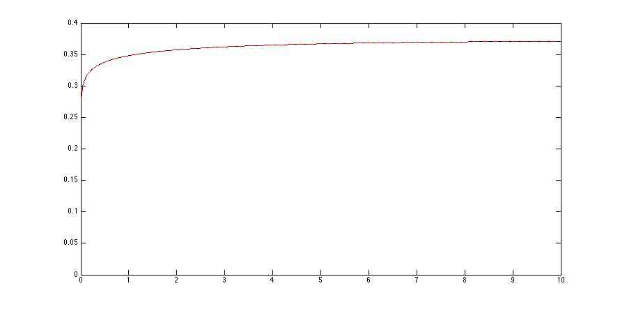
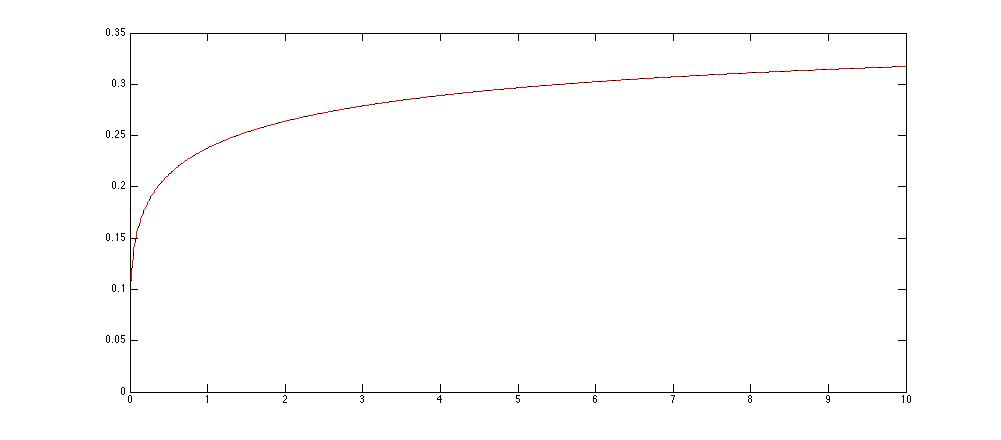
Numerical aspects of this equation in the “rough setting”, that is for kernels K=KαK=K_{\alpha}, α=H+12\alpha=H+\frac{1}{2} with H∈(0,12)H\!\in(0,\frac{1}{2}), and for a specific family of diffusion coefficients σ⁡(x)=κ0+κ1​(x−μ0λ)+κ2​(x−μ0λ)2\sigma(x)=\sqrt{\kappa_{0}+\kappa_{1}(x-\frac{\mu_{0}}{\lambda})+\kappa_{2}(x-\frac{\mu_{0}}{\lambda})^{2}}, are investigated in Section 5.1 where theoretical results are established like the square integrability of fλf_{\lambda} and the existence of a continuous bounded stabilizer ςλ,c\varsigma_{\lambda,c}, null at 00 and positive on (0,+∞)(0,+\infty)

3.2 Fake stationary regimes of types I and II: first properties and examples

Before exploring the main two situations for σ\sigma, let us come back to the notion of fake stationary regime of type I. The following proposition emphasizes that there is in fact an equivalence between having a constant variance and a constant value for 𝔼​σ2​(Xt){\mathbb{E}}\,\sigma^{2}(X_{t}).

Proposition 3.2 (An equivalence)

Let λ>0\lambda>0, let μ0∈ℝ\mu_{0}\!\in{\mathbb{R}} and let σ:ℝ→ℝ\sigma:{\mathbb{R}}\to{\mathbb{R}} be a Lipschitz continuous function. Let X0∈L2​(Ω,𝒜,ℙ)X_{0}\!\in L^{2}(\Omega,{\cal A},{\mathbb{P}}) be such that 𝔼​X0=μ0λ{\mathbb{E}}\,X_{0}=\frac{\mu_{0}}{\lambda} and Var⁡(X0)=v0≥0{\rm Var}(X_{0})=v_{0}\geq 0. Set σ¯02=𝔼​σ2​(X0)>0\bar{\sigma}_{0}^{2}={\mathbb{E}}\,\sigma^{2}(X_{0})>0 and set c=v0σ¯02∈ℝ+c=\frac{v_{0}}{\bar{\sigma}_{0}^{2}}\!\in{\mathbb{R}}_{+}. Assume the kernel KK satisfies (1.2), (1.3), fλ2f^{2}_{\lambda} has a finite Laplace transform on (0,+∞)(0,+\infty) and (Eλ)(E_{\lambda}) is in force.

Then, the unique strong solution starting from X0X_{0} of the scaled Volterra equation (3.27) where ςλ,c\varsigma_{\lambda,c} is solution to (3.28) (has constant mean) and) satisfies the following equivalence between the following two claims:

(i)(i) ∀t≥0\forall\,t\geq 0, Var⁡(Xt)=Var⁡(X0)=v0{\rm Var}(X_{t})={\rm Var}(X_{0})=v_{0},

(i​i)(ii) ∀t≥0\forall\,t\geq 0, 𝔼​σ2​(Xt)=𝔼​σ2​(X0)=σ¯02{\mathbb{E}}\,\sigma^{2}(X_{t})={\mathbb{E}}\,\sigma^{2}(X_{0})=\bar{\sigma}_{0}^{2}.

Proof. We just have to prove the equivalence.

(i​i)⇒(i)(ii)\Rightarrow(i) Then σ¯2=σ¯t2=𝔼​σ2​(Xt)\bar{\sigma}^{2}=\bar{\sigma}^{2}_{t}={\mathbb{E}}\,\sigma^{2}(X_{t}), t≥0t\geq 0, so that, having in mind that c=v0σ¯02=v0σ¯2c=\frac{v_{0}}{\bar{\sigma}^{2}_{0}}=\frac{v_{0}}{\bar{\sigma}^{2}}, it follows from Equation (3.28) that

Var⁡(Xt)\displaystyle{\rm Var}(X_{t}) =Var⁡(X0)​Rλ2​(t)+σ¯2λ2​fλ2∗ςλ,c2\displaystyle={\rm Var}(X_{0})R^{2}_{\lambda}(t)+\frac{\bar{\sigma}^{2}}{\lambda^{2}}f^{2}_{\lambda}*\varsigma_{\lambda,c}^{2}
=Var⁡(X0)​Rλ2​(t)+v0c​λ2​fλ2∗ςλ,c2\displaystyle={\rm Var}(X_{0})R^{2}_{\lambda}(t)+\frac{v_{0}}{c\lambda^{2}}f^{2}_{\lambda}*\varsigma_{\lambda,c}^{2}
=v0​Rλ2​(t)+(1−Rλ2​(t))​v0=v0.\displaystyle=v_{0}R^{2}_{\lambda}(t)+\big(1-R^{2}_{\lambda}(t)\big)v_{0}=v_{0}.

(i)⇒(i​i)(i)\Rightarrow(ii) Assume Var⁡(Xt)=Var⁡(X0)=v0{\rm Var}(X_{t})={\rm Var}(X_{0})=v_{0} for every t≥0t\geq 0.

If v0=0v_{0}=0, then Xt=μ0λX_{t}=\frac{\mu_{0}}{\lambda} a.s.a.s. for every t≥0t\geq 0. Consequently 𝔼​σ2​(Xt)=σ2​(μ0λ){\mathbb{E}}\,\sigma^{2}(X_{t})=\sigma^{2}\big(\frac{\mu_{0}}{\lambda}\big), t≥0t\geq 0.

If v0>0v_{0}>0, c∈(0,+∞)c\!\in(0,+\infty) since σ¯02=𝔼​σ2​(X0)>0\bar{\sigma}^{2}_{0}={\mathbb{E}}\,\sigma^{2}(X_{0})>0. Then, one checks using (2.19) that the function

y⁡(t)=ςλ,c2​(t)​(𝔼​σ2​(Xt)σ¯02−1)y(t)=\varsigma^{2}_{\lambda,c}(t)\Big(\frac{{\mathbb{E}}\,\sigma^{2}(X_{t})}{\bar{\sigma}^{2}_{0}}-1\Big)

is solution to fλ2∗y=0f^{2}_{\lambda}*y=0 and satisfies y⁡(0)=0y(0)=0 since ςλ,c\varsigma_{\lambda,c} is bounded by assumption and t↦𝔼​σ2​(Xt)t\mapsto{\mathbb{E}}\,\sigma^{2}(X_{t}) is continuous. Moreover by the linear growth assumption on σ\sigma, we know that 𝔼​σ2​(Xt){\mathbb{E}}\,\sigma^{2}(X_{t}) is bounded since 𝔼​Xt2{\mathbb{E}}\,X_{t}^{2} is. Consequently yy has a Laplace transform as well as its positive and negative parts y±y^{\pm}. One has Lfλ2⋅Ly+=Lfλ2⋅Ly−L_{f^{2}_{\lambda}}\cdot L_{y^{+}}=L_{f^{2}_{\lambda}}\cdot L_{y^{-}}. If Lfλ2L_{f^{2}_{\lambda}} is not identically 00, then it is positive on (0,+∞)(0,+\infty) so that Ly+=Ly−L_{y^{+}}=L_{y^{-}} which implies y+=y−y^{+}=y^{-}, hence y=0y=0. □\Box

This result does not presume of the existence of a fake stationary regime of type I, but that to establish its existence, it suffices to check that both mean and variance are constant.

3.2.1 The case σ⁡(x)=σ\sigma(x)=\sigma

Then under the assumptions of Proposition 3.2 one easily checks that σ¯02=σ2\bar{\sigma}_{0}^{2}=\sigma^{2} and that the solution (Xt)t≥0(X_{t})_{t\geq 0} to (3.27) with c=v0σ2c=\frac{v_{0}}{\sigma^{2}} has constant mean μ0λ\frac{\mu_{0}}{\lambda} and variance v0v_{0}. As a consequence, if X0∼𝒩⁡(μ0λ,v0)X_{0}\sim{\cal N}\big(\frac{\mu_{0}}{\lambda},v_{0}\big), then Xt∼X0X_{t}\sim X_{0} for every t≥0t\geq 0 i.e. XX has a fake stationary regime of type II since the process becomes clearly Gaussian. All this follows from the identity:

∀s,t≥0,Cov⁡(Xt,Xs)=v0​(Rλ​(t)​Rλ​(s)+1λ2​c​∫0t∧sfλ​(t−u)​fλ​(s−u)​ςλ,c2​(u)​𝑑u).\forall\,s,\,t\geq 0,\quad{\rm Cov}(X_{t},X_{s})=v_{0}\Big(R_{\lambda}(t)R_{\lambda}(s)+\frac{1}{\lambda^{2}c}\int_{0}^{t\wedge s}f_{\lambda}(t-u)f_{\lambda}(s-u)\varsigma^{2}_{\lambda,c}(u)du\Big).

3.2.2 Trinomial squared volatility

In this section we specify a family of stabilized scaled Volterra equations (3.27) where

σ⁡(x)=κ0+κ1​(x−μ0λ)+κ2​(x−μ0λ)2 with κi≥0,i=1,2,κ12≤4​κ0​κ2,\sigma(x)=\sqrt{\kappa_{0}+\kappa_{1}\,(x-\tfrac{\mu_{0}}{\lambda})+\kappa_{2}\,(x-\tfrac{\mu_{0}}{\lambda})^{2}}\quad\mbox{ with }\quad\kappa_{i}\geq 0,\;i=1,2,\;\kappa^{2}_{1}\leq 4\kappa_{0}\kappa_{2}, (3.30)

for which we will establish the existence of a fake stationary regime (of type I in general). Note that κ1=0\kappa_{1}=0 whenever κ0\kappa_{0} or κ2=0\kappa_{2}=0 and that

κ2=[σ]Lip2 and σ⁡(μ0λ)=κ0.\kappa_{2}=[\sigma]^{2}_{\rm Lip}\quad\mbox{ and }\quad\sigma\big(\tfrac{\mu_{0}}{\lambda}\big)=\kappa_{0}.

This is this type of vol-vol term that appears in the quadratic rough volatility model introduced in [12] to solve the problem of the joint S&P 500/VIX smile calibration problem.

Proposition 3.3 (Fake stationary regimes (types I and II) and first asymptotics)

Consider the stabilized Volterra Equation (3.27) with λ>0\lambda>0, μ0∈ℝ\mu_{0}\!\in{\mathbb{R}}, where σ\sigma is given by (3.30) and ς=ςλ,c\varsigma=\varsigma_{\lambda,c}, assumed to be the unique continuous solution to Equation (3.28) for some c∈(0,1κ2)c\in(0,\frac{1}{\kappa_{2}}) (so that condition (Eλ)(E_{\lambda}) is satisfied). Then, let X0∈L2​(ℙ)X_{0}\!\in L^{2}({\mathbb{P}}) with

𝔼​X0=μ0λ and v0=Var⁡(X0)=c​κ01−c​κ2.{\mathbb{E}}\,X_{0}=\frac{\mu_{0}}{\lambda}\quad\mbox{ and }\quad v_{0}={\rm Var}(X_{0})=\frac{c\kappa_{0}}{1-c\kappa_{2}}.

(a)(a) Case κ2>0\kappa_{2}>0. The solution (Xt)t≥0(X_{t})_{t\geq 0} to (3.27) has a fake stationary regime of type I i.e.

∀t≥0,𝔼​Xt=μ0λ,Var⁡(Xt)=v0=c​κ01−c​κ2​ and 𝔼​σ2​(Xt)=σ¯02=κ01−c​κ2.\forall\,t\geq 0,\qquad{\mathbb{E}}\,X_{t}=\frac{\mu_{0}}{\lambda},\quad{\rm Var}(X_{t})=v_{0}=\frac{c\kappa_{0}}{1-c\kappa_{2}}\mbox{ and }\quad{\mathbb{E}}\,\sigma^{2}(X_{t})=\bar{\sigma}_{0}^{2}=\frac{\kappa_{0}}{1-c\kappa_{2}}.

Moreover, for any starting value X0∈L2​(ℙ)X_{0}\!\in L^{2}({\mathbb{P}}),

𝔼​Xt→μ0λ and Var⁡(Xt)→c​κ01−c​κ2 as ​t→+∞.{\mathbb{E}}\,X_{t}\to\frac{\mu_{0}}{\lambda}\quad\mbox{ and }\quad{\rm Var}(X_{t})\to\frac{c\kappa_{0}}{1-c\kappa_{2}}\quad\mbox{ as }t\to+\infty.

(b)(b) Case κ2=0\kappa_{2}=0. Then κ1=0\kappa_{1}=0, σ⁡(x)=κ0\sigma(x)=\sqrt{\kappa_{0}} is constant (the choice of c>0c>0 becomes free) and if X0∼ν:=𝒩⁡(μ0λ,c​κ01−c​κ2)X_{0}\sim\nu:={\mathcal{N}}\big(\frac{\mu_{0}}{\lambda},\frac{c\kappa_{0}}{1-c\kappa_{2}}\big), then (Xt)t≥0(X_{t})_{t\geq 0} is a Gaussian process with a fake stationary regime of type II with ν\nu as 11-marginal distribution

Practitioner’s corner. ∙\bullet The above proposition covers at least partially the rough volatility dynamics recently introduced in [12] (the volatility process being defined as Vt=σ⁡(Xt)V_{t}=\sigma(X_{t}) with our notations). In this model, the traded asset and its volatility are driven by the same Brownian motion and its purpose is to propose a joint calibration of the VIX and the SP500 in order to take into account the so-called Zumbach effect which connects the evolution of the asset (here an index) and its volatility.

∙\bullet Note that in practice, when κ1>0\kappa_{1}>0, if we fix the value of v0v_{0}, then c=v0κ0+v0​κ2c=\frac{v_{0}}{\kappa_{0}+v_{0}\kappa_{2}} so that, σ\sigma being κ2\sqrt{\kappa_{2}}-Lipschitz continuous, one has κ2​[σ]Lip2=v0​κ2κ0+v0​κ2<1\kappa_{2}[\sigma]^{2}_{\rm Lip}=\frac{v_{0}\kappa_{2}}{\kappa_{0}+v_{0}\kappa_{2}}<1 which ensures the L2L^{2}-confluence of the paths of the solution (see Proposition 4.3 further on).

Remark. If we consider a dynamics more inspired by the original CIR model in which μ⁡(t)=μ0>0\mu(t)=\mu_{0}>0, σ⁡(t,x)=ςλ,c​(t)​σ​(x)\sigma(t,x)=\varsigma_{\lambda,c}(t)\sigma(x) with σ⁡(x):=κ0+κ1​(x−μ0λ)\sigma(x):=\sqrt{\kappa_{0}+\kappa_{1}(x-\frac{\mu_{0}}{\lambda})}, κ1>0\kappa_{1}>0, κ0>κ1​μ0λ\kappa_{0}>\kappa_{1}\frac{\mu_{0}}{\lambda}, the resulting Volterra equation (2.18) may have (at least) a non-negative weak solution e.g. as the CC-weak limit of a system of Hawkes processes (as it has been done in [16] without the presence of the corrector ςλ,c\varsigma_{\lambda,c}, see also [14], [1]). If such a non-negative weak solution on the whole non-negative real line does exists starting from X0X_{0} with mean μ0λ\frac{\mu_{0}}{\lambda} then

Var⁡(Xt)=Var⁡(X0)​Rλ2​(t)+κ0​(1−Rλ2​(t)).{\rm Var}(X_{t})={\rm Var}(X_{0})R^{2}_{\lambda}(t)+\kappa_{0}\big(1-R^{2}_{\lambda}(t)\big).

A fake stationary regime of type I then should have constant mean 𝔼​Xt=μ0λ{\mathbb{E}}\,X_{t}=\frac{\mu_{0}}{\lambda} and a variance given by Var⁡(Xt)=c​κ0{\rm Var}(X_{t})=c\kappa_{0} respectively and one easily checks that such is the case. Note that if κ0=0\kappa_{0}=0 – like in the Volterra CIR like model – one retrieves the degenerate situation where Xt=μ0λX_{t}=\frac{\mu_{0}}{\lambda} ℙ{\mathbb{P}}-a.s.a.s.

Proof. (a)(a) Note that, if κ2>0\kappa_{2}>0, [σ]Lip=κ2[\sigma]_{\rm Lip}=\sqrt{\kappa_{2}} since

σ⁡(x)=κ2​(x−μ0λ−κ12​κ2)2+κ0−κ124​κ2\sigma(x)=\sqrt{\kappa_{2}\big(x-\tfrac{\mu_{0}}{\lambda}-\frac{\kappa_{1}}{2\kappa_{2}}\big)^{2}+\kappa_{0}-\frac{\kappa_{1}^{2}}{4\kappa_{2}}}

so that the condition 0<c<1/[σ]Lip20<c<1/[\sigma]^{2}_{\rm Lip} is satisfied. We know that

𝔼​Xt=μ0λ​Rλ2​(t)+μ0λ​(1−Rλ2​(t))=μ0λ{\mathbb{E}}\,X_{t}=\frac{\mu_{0}}{\lambda}R_{\lambda}^{2}(t)+\frac{\mu_{0}}{\lambda}(1-R^{2}_{\lambda}(t))=\frac{\mu_{0}}{\lambda}

for every t≥0t\geq 0. As for the variance, we have

Var⁡(Xt)\displaystyle{\rm Var}(X_{t}) =Var⁡(X0)​Rλ2​(t)+1λ2​fλ2∗(ς2​𝔼​σ2​(X⋅))t\displaystyle={\rm Var}(X_{0})R^{2}_{\lambda}(t)+\frac{1}{\lambda^{2}}f^{2}_{\lambda}*\big(\varsigma^{2}\,{\mathbb{E}}\,\sigma^{2}(X_{\cdot})\big)_{t}
=Var⁡(X0)​Rλ2​(t)+κ0λ2​(fλ2∗ς2)t+κ1×0+κ2λ2​fλ2∗(ς2​Var​(X⋅))t.\displaystyle={\rm Var}(X_{0})R^{2}_{\lambda}(t)+\frac{\kappa_{0}}{\lambda^{2}}(f^{2}_{\lambda}*\varsigma^{2})_{t}+\kappa_{1}\times 0+\frac{\kappa_{2}}{\lambda^{2}}f^{2}_{\lambda}*\big(\varsigma^{2}\,{\rm Var}(X_{\cdot})\big)_{t}. (3.31)

If we assume that Var⁡(Xt){\rm Var}(X_{t}) is constant i.e. Var⁡(Xt)=v0{\rm Var}(X_{t})=v_{0} for every t≥0t\geq 0 and take advantage of the identity (3.28) satisfied by ς=ςλ,c\varsigma=\varsigma_{\lambda,c}, the above equation reads

v0​(1−Rλ2​(t))=(c​κ0+c​κ2​v0)​(1−Rλ2​(t)),t≥0v_{0}(1-R^{2}_{\lambda}(t))=(c\kappa_{0}+c\kappa_{2}v_{0})(1-R^{2}_{\lambda}(t)),\quad t\geq 0

i.e.

v0=c​κ01−c​κ2>0v_{0}=\frac{c\kappa_{0}}{1-c\kappa_{2}}>0

since Rλ​(t)>1R_{\lambda}(t)>1 for tt large enough ,which is clearly solution to the equation.

Conversely one checks that this constant value for the variance solves the above equation. Let us prove that it is the only one. By the linearity of Equation (3.31), it suffices to show that the equation in x∈𝒞⁡(ℝ+,ℝ)x\!\in{\cal C}({\mathbb{R}}_{+},{\mathbb{R}})

x(t)=κ2λ2(fλ2∗(ς2.x))t,x(0)=0x(t)=\frac{\kappa_{2}}{\lambda^{2}}\big(f^{2}_{\lambda}*(\varsigma^{2}.\,x)\big)_{t},\quad x(0)=0

only has the null function as solution. If xx solves the above equation, then

|x⁡(t)|≤κ2λ2​(fλ2∗ς2)t​sup0≤s≤t|x⁡(s)|=c​κ2​sup0≤s≤t|x⁡(s)|.|x(t)|\leq\frac{\kappa_{2}}{\lambda^{2}}(f^{2}_{\lambda}*\varsigma^{2})_{t}\sup_{0\leq s\leq t}|x(s)|\,=c\kappa_{2}\sup_{0\leq s\leq t}|x(s)|.

If x≡/ 0x\equiv\!\!\!\!\!/\,0, there exist ε>0\varepsilon>0 such that τε=inf{t:|x⁡(t)|>ε}<+∞\tau_{\varepsilon}=\inf\{t:|x(t)|>\varepsilon\}<+\infty. By continuity of xx it is clear that τε>0\tau_{\varepsilon}>0 and |x(τε)|=sup0:≤s≤t|x(s)|=ε|x(\tau_{\varepsilon})|=\sup_{0:\leq s\leq t}|x(s)|=\varepsilon which is impossible since κ2​c<1\kappa_{2}c<1. Consequently x≡0x\equiv 0.

Hence (Xt)t≥0(X_{t})_{t\geq 0} is a fake stationary regime of type II with the above mean and variance. The last claim is a straightforward consequence of Proposition 4.3.

(b)(b) is obvious once noted that (Xt)t≥0(X_{t})_{t\geq 0} is a Gaussian process (and [σ]Lip=0[\sigma]_{\rm Lip}=0). □\Box

4 Long run behaviour : asymptotics and confluence

In this section we try to answer the question; “How does the process (Xt)t≥(X_{t})_{t\geq} behave when tt goes to infinity and possibly starting from any X0∈Lp​(ℙ)X_{0}\!\in L^{p}({\mathbb{P}}), p=2p=2 or p>2p>2 ?”

We first recall a result on the constant of an LpL^{p}-Burkholder-Davis-Gundy (BDG) inequality.

Lemma 4.1 (Best constant in a BDG inequality (see Remark 2 in [5]))

Let MM be a continuous local martingale null at t=0t=0. Then, for every p≥1p\geq 1

‖Mt‖p≤2​p​‖⟨M⟩12‖p.\|M_{t}\|_{p}\leq 2\sqrt{p}\,\|\langle M\rangle^{\frac{1}{2}}\|_{p}.
Proposition 4.2 (Moment control)

Let λ,c>0\lambda,c>0, let μ0∈ℝ\mu_{0}\!\in{\mathbb{R}}, and let σ:ℝ→ℝ\sigma:{\mathbb{R}}\to{\mathbb{R}} be a Lipschitz continuous function. Assume (Eλ)(E_{\lambda}) is in force and ςλ,c\varsigma_{\lambda,c} is continuous. Assume fλ∈ℒ2​(Leb1)f_{\lambda}\!\in{\cal L}^{2}({\rm Leb}_{1}). Let (Xt)t≥0(X_{t})_{t\geq 0} be a solution to the scaled Volterra equation in its form (3.27) starting from any X0∈L2​(ℙ)X_{0}\!\in L^{2}({\mathbb{P}}).

(a)(a) First two moments. Assume c∈(0,1[σ]Lip2)c\!\in\big(0,\frac{1}{[\sigma]^{2}_{\rm Lip}}\big). Then, one has

|𝔼​Xt−μ0λ|≤Rλ​(t)​|𝔼​X0−μ0λ|,t≥0\Big|{\mathbb{E}}\,X_{t}-\frac{\mu_{0}}{\lambda}\Big|\leq R_{\lambda}(t)\Big|{\mathbb{E}}\,X_{0}-\frac{\mu_{0}}{\lambda}\Big|,\quad t\geq 0

and

supt≥0‖Xt−μ0λ‖2≤[c1−[σ]Lip​c​|σ⁡(μ0λ)|]∨‖X0−μ0λ‖2<+∞.\sup_{t\geq 0}\Big\|X_{t}-\frac{\mu_{0}}{\lambda}\Big\|_{2}\leq\left[\frac{\sqrt{c}}{1-[\sigma]_{\rm Lip}\sqrt{c}}\big|\sigma(\tfrac{\mu_{0}}{\lambda})\big|\right]\vee\Big\|X_{0}-\frac{\mu_{0}}{\lambda}\Big\|_{2}<+\infty.

(b)(b) LpL^{p}-moments, p∈(2,+∞)p\!\in(2,+\infty). If furthermore X0∈Lp​(ℙ)X_{0}\!\in L^{p}({\mathbb{P}}) and c∈(0,14​p​[σ]Lip2)c\!\in\big(0,\frac{1}{4p[\sigma]^{2}_{\rm Lip}}\big) then

supt≥0‖Xt−μ0λ‖p≤infϵ∈(0,14​c​p​[σ]Lip2−1)([2​p​c​(1+ϵ)1−2​[σ]Lip​p​c​(1+ϵ)​|σ⁡(μ0λ)|]∨[(1+1/ϵ)12​‖X0−μ0λ‖p])<+∞.\sup_{t\geq 0}\Big\|X_{t}-\frac{\mu_{0}}{\lambda}\Big\|_{p}\leq\inf_{\epsilon\in(0,\frac{1}{4cp[\sigma]_{\rm Lip}^{2}}-1)}\bigg(\left[\frac{2\sqrt{pc(1+\epsilon)}}{1-2[\sigma]_{\rm Lip}\sqrt{pc(1+\epsilon)}}\big|\sigma(\tfrac{\mu_{0}}{\lambda})\big|\right]\vee\left[(1+1/\epsilon)^{\frac{1}{2}}\Big\|X_{0}-\frac{\mu_{0}}{\lambda}\Big\|_{p}\right]\bigg)<+\infty.

Remark. If |σ⁡(x)|2≤κ0+κ2​(x−μ0λ)2|\sigma(x)|^{2}\leq\kappa_{0}+\kappa_{2}(x-\frac{\mu_{0}}{\lambda})^{2} is a Borel function, the above results remain valid by simply replacing [σ]Lip2[\sigma]^{2}_{\rm Lip} by κ2\kappa_{2} if (2.18) has a solution.

Proof. (a)(a) Set ρ:=c​[σ]Lip2∈(0,1)\rho:=c[\sigma]^{2}_{\rm Lip}\!\in(0,1) and let η∈(0,1−ρ)\eta\in(0,1-\rho) be a free parameter such that ρ+η∈(0,1)\rho+\eta\!\in(0,1). One has for every x∈ℝx\!\in{\mathbb{R}},

σ2​(x)≤(|σ⁡(μ0λ)|+[σ]Lip​|x−μ0λ|)2≤κ0+κ2​|x−μ0λ|2\sigma^{2}(x)\leq\big(\big|\sigma(\tfrac{\mu_{0}}{\lambda})\big|+[\sigma]_{\rm Lip}\big|x-\tfrac{\mu_{0}}{\lambda}|\big)^{2}\leq\kappa_{0}+\kappa_{2}\big|x-\tfrac{\mu_{0}}{\lambda}|^{2} (4.32)

with real constant κi\kappa_{i}, i=0,2i=0,2 depending on η\eta and reading

κ0=κ0​(η)=(1+ρ​η−1)​|σ⁡(μ0λ)|2 andκ2=κ2​(η)=[σ]Lip2​(1+η​ρ−1)\kappa_{0}=\kappa_{0}(\eta)=(1+\rho\eta^{-1})|\sigma(\tfrac{\mu_{0}}{\lambda})|^{2}\quad\mbox{ and}\quad\kappa_{2}=\kappa_{2}(\eta)=[\sigma]_{\rm Lip}^{2}(1+\eta\rho^{-1})

so that c​κ2=ρ+η<1c\kappa_{2}=\rho+\eta<1. Using that fλ2∗ς2=c​λ2​(1−Rλ2)f^{2}_{\lambda}*\varsigma^{2}=c\lambda^{2}(1-R^{2}_{\lambda}) elementary computations show that for every t≥0t\geq 0

𝔼​(Xt−μ0λ)2≤𝔼​(X0−μ0λ)2​Rλ2​(t)+κ1​(1−Rλ2​(t))+κ2λ2​∫0tfλ2​(t−s)​ς2​(s)​𝔼​(Xs−μ0λ)2​𝑑s{\mathbb{E}}\,\Big(X_{t}-\frac{\mu_{0}}{\lambda}\Big)^{2}\leq{\mathbb{E}}\,\Big(X_{0}-\frac{\mu_{0}}{\lambda}\Big)^{2}R^{2}_{\lambda}(t)+\kappa_{1}\big(1-R^{2}_{\lambda}(t)\big)+\frac{\kappa_{2}}{\lambda^{2}}\int_{0}^{t}f^{2}_{\lambda}(t-s)\varsigma^{2}(s){\mathbb{E}}\,\Big(X_{s}-\frac{\mu_{0}}{\lambda}\Big)^{2}ds (4.33)

Now let A>A¯η:=κ0​c1−κ2​c∨𝔼​(X0−μ0λ)2A>\bar{A}_{\eta}:=\frac{\kappa_{0}c}{1-\kappa_{2}c}\vee{\mathbb{E}}\,\Big(X_{0}-\frac{\mu_{0}}{\lambda}\Big)^{2}, δ>0\delta>0 and

tδ=inf{t:𝔼​(Xt−μ0λ)2≥A+δ}.t_{\delta}=\inf\Big\{t:{\mathbb{E}}\,\Big(X_{t}-\frac{\mu_{0}}{\lambda}\Big)^{2}\geq A+\delta\Big\}.

As t↦𝔼​(Xt−μ0λ)2t\mapsto{\mathbb{E}}\,\Big(X_{t}-\frac{\mu_{0}}{\lambda}\Big)^{2} is continuous and A>𝔼​(X0−μ0λ)2A>{\mathbb{E}}\,\Big(X_{0}-\frac{\mu_{0}}{\lambda}\Big)^{2} it follows from the above inequality and the identity satisfied by ς\varsigma that, if tδ<+∞t_{\delta}<+\infty,

A+δ=𝔼​(Xtδ−μ0λ)2<A​Rλ2​(tδ)+(κ0​c+κ2​c​(A+δ))​(1−Rλ2​(tδ)).A+\delta={\mathbb{E}}\,\Big(X_{t_{\delta}}-\frac{\mu_{0}}{\lambda}\Big)^{2}<AR^{2}_{\lambda}(t_{\delta})+\big(\kappa_{0}c+\kappa_{2}c(A+\delta)\big)\big(1-R^{2}_{\lambda}(t_{\delta})\big).

Now, we have κ0​c+κ2​c​A<A\kappa_{0}c+\kappa_{2}cA<A by construction of AA, hence

A+δ=𝔼​(Xtδ−μ0λ)2<A​Rλ2​(tδ)+A⁡(1−Rλ2​(tδ))+κ2​c​δ​((1−Rλ2​(tδ))<A+δCLOSE.A+\delta={\mathbb{E}}\,\Big(X_{t_{\delta}}-\frac{\mu_{0}}{\lambda}\Big)^{2}<AR^{2}_{\lambda}(t_{\delta})+A(1-R^{2}_{\lambda}(t_{\delta}))+\kappa_{2}c\delta\big((1-R^{2}_{\lambda}(t_{\delta})\big)<A+\delta.

which yields a contradiction. Consequently, tδ=+∞t_{\delta}=+\infty which implies that 𝔼​(Xt−μ0λ)2≤A+δ{\mathbb{E}}\,\Big(X_{t}-\frac{\mu_{0}}{\lambda}\Big)^{2}\leq A+\delta for every t≥0t\geq 0. Letting δ→0\delta\to 0 and A→A¯ηA\to\bar{A}_{\eta} successively, yields

supt≥0𝔼​(Xt−μ0λ)2≤A¯η=c​|σ⁡(μ0λ)|2​η+ρη⁡(1−ρ−η).\sup_{t\geq 0}{\mathbb{E}}\,\Big(X_{t}-\frac{\mu_{0}}{\lambda}\Big)^{2}\leq\bar{A}_{\eta}=c|\sigma(\tfrac{\mu_{0}}{\lambda})|^{2}\frac{\eta+\rho}{\eta(1-\rho-\eta)}.

Then one checks that η↦A¯η\eta\mapsto\bar{A}_{\eta} is minimal over (0,1−ρ)(0,1-\rho) at η=ρ−ρ\eta=\sqrt{\rho}-\rho which finally yields the announced result.

(b)(b) Let p≥2p\geq 2. Set ρp:=c​Cp2​[σ]Lip2<1\rho_{p}:=c\,C^{2}_{p}[\sigma]_{\rm Lip}^{2}<1. Using successively BDG inequality to the (a priori) local martingale Ms=∫0sfλ​(t−u)​ζ​(u)​σ​(Xu)​d​WuM_{s}=\int_{0}^{s}f_{\lambda}(t-u)\zeta(u)\sigma(X_{u})dW_{u}, 0≤s≤t0\leq s\leq t, (see [23, Proposition 4.3]) and the generalized Minkowski inequality, we get

‖Xt−μ0λ‖p\displaystyle\Big\|X_{t}-\frac{\mu_{0}}{\lambda}\Big\|_{p} ≤‖X0−μ0λ‖p​Rλ​(t)+Cpλ​‖∫0tfλ2​(t−s)​ς2​(s)​σ​(Xs)2​𝑑s‖p212\displaystyle\leq\Big\|X_{0}-\frac{\mu_{0}}{\lambda}\Big\|_{p}R_{\lambda}(t)+\frac{C_{p}}{\lambda}\Big\|\int_{0}^{t}f^{2}_{\lambda}(t-s)\varsigma^{2}(s)\sigma(X_{s})^{2}ds\Big\|_{\frac{p}{2}}^{\frac{1}{2}}
≤‖X0−μ0λ‖p​Rλ​(t)+Cpλ​(∫0tfλ2​(t−s)​ς2​(s)​‖σ⁡(Xs)‖p2)12\displaystyle\leq\Big\|X_{0}-\frac{\mu_{0}}{\lambda}\Big\|_{p}R_{\lambda}(t)+\frac{C_{p}}{\lambda}\Big(\int_{0}^{t}f^{2}_{\lambda}(t-s)\varsigma^{2}(s)\|\sigma(X_{s})\|^{2}_{p}\Big)^{\frac{1}{2}}

(with an equality when p=2p=2 in the first line). Now let ϵ∈(0,1/ρp−1)\epsilon\!\in(0,1/\rho_{p}-1). It follows from the elementary inequality (a+b)2≤(1+1/ϵ)​a2+(1+ϵ)​b2(a+b)^{2}\leq(1+1/\epsilon)a^{2}+(1+\epsilon)b^{2} that

‖Xt−μ0λ‖p2≤‖X0−μ0λ‖p2​Rλ2​(t)​(1+1/ϵ)+Cp2λ2​(1+ϵ)​∫0tfλ2​(t−s)​ς2​(s)​‖σ​(Xs)2‖p2​𝑑s.\Big\|X_{t}-\frac{\mu_{0}}{\lambda}\Big\|_{p}^{2}\leq\Big\|X_{0}-\frac{\mu_{0}}{\lambda}\Big\|^{2}_{p}R^{2}_{\lambda}(t)(1+1/\epsilon)+\frac{C^{2}_{p}}{\lambda^{2}}(1+\epsilon)\int_{0}^{t}f^{2}_{\lambda}(t-s)\varsigma^{2}(s)\|\sigma(X_{s})^{2}\|_{\frac{p}{2}}ds.

Let ρ~p=ρp​(1+ϵ)∈(0,1)\tilde{\rho}_{p}=\rho_{p}(1+\epsilon)\!\in(0,1) and for η∈(0,1−ρ~p)\eta\!\in(0,1-\tilde{\rho}_{p}), set now κi\kappa_{i} depending on η\eta and reading

κ0=κ1​(η)=(1+ρ~p​η−1)​|σ⁡(μ0λ)|2 andκ2=κ2​(η)=[σ]Lip2​(1+η​ρ~p−1)\kappa_{0}=\kappa_{1}(\eta)=(1+\tilde{\rho}_{p}\eta^{-1})|\sigma(\tfrac{\mu_{0}}{\lambda})|^{2}\quad\mbox{ and}\quad\kappa_{2}=\kappa_{2}(\eta)=[\sigma]_{\rm Lip}^{2}(1+\eta\tilde{\rho}_{p}^{-1})

so that c​Cp2​(1+ϵ)​κ2=ρ~p+η<1c\,C^{2}_{p}(1+\epsilon)\kappa_{2}=\tilde{\rho}_{p}+\eta<1. As p2≥1\frac{p}{2}\geq 1, it follows from (4.32) that

‖σ⁡(Xs)‖p2=‖σ​(Xs)2‖p2≤κ0+κ2​‖Xs−μ0λ‖p2\|\sigma(X_{s})\|^{2}_{p}=\|\sigma(X_{s})^{2}\|_{\frac{p}{2}}\leq\kappa_{0}+\kappa_{2}\Big\|X_{s}-\frac{\mu_{0}}{\lambda}\Big\|^{2}_{p}

which entails, combined with the identity fλ2∗ς2=c​λ2​(1−Rλ2)f^{2}_{\lambda}*\varsigma^{2}=c\lambda^{2}(1-R^{2}_{\lambda}), that, for every t≥0t\geq 0,

‖Xt−μ0λ‖p2\displaystyle\Big\|X_{t}-\frac{\mu_{0}}{\lambda}\Big\|_{p}^{2} ≤‖X0−μ0λ‖p2​Rλ2​(t)​(1+1/ϵ)+Cp2​(1+ϵ)​(κ1​c​(1−Rλ2​(t))CLOSE\displaystyle\leq\Big\|X_{0}-\frac{\mu_{0}}{\lambda}\Big\|_{p}^{2}R^{2}_{\lambda}(t)(1+1/\epsilon)+C_{p}^{2}(1+\epsilon)\Big(\kappa_{1}c\big(1-R^{2}_{\lambda}(t)\big)
+κ2λ2∫0tfλ2(t−s)ς2(s)∥Xs−μ0λ∥p2ds).\displaystyle\qquad+\frac{\kappa_{2}}{\lambda^{2}}\int_{0}^{t}f^{2}_{\lambda}(t-s)\varsigma^{2}(s)\Big\|X_{s}-\frac{\mu_{0}}{\lambda}\Big\|^{2}_{p}ds\Big). (4.34)

Now let A>A¯η,ϵ:=κ0​c​Cp2​(1+ϵ)1−κ2​c​Cp2​(1+ϵ)∨[(1+1/ϵ)​‖X0−μ0λ‖p2]A>\bar{A}_{\eta,\epsilon}:=\frac{\kappa_{0}c\,C_{p}^{2}(1+\epsilon)}{1-\kappa_{2}c\,C_{p}^{2}(1+\epsilon)}\vee\Big[(1+1/\epsilon)\Big\|X_{0}-\frac{\mu_{0}}{\lambda}\Big\|_{p}^{2}\Big], δ>0\delta>0 and

tδ=inf{t:‖Xt−μ0λ‖p2≥A+δ}.t_{\delta}=\inf\Big\{t:\Big\|X_{t}-\frac{\mu_{0}}{\lambda}\Big\|_{p}^{2}\geq A+\delta\Big\}.

If tδ<+∞t_{\delta}<+\infty, it follows on the one hand from the continuity of t↦‖Xt−μ0λ‖p2t\mapsto\Big\|X_{t}-\frac{\mu_{0}}{\lambda}\Big\|_{p}^{2} that A+δ=‖Xtδ−μ0λ‖p2A+\delta=\Big\|X_{t_{\delta}}-\frac{\mu_{0}}{\lambda}\Big\|_{p}^{2} and, on the other hand, from Equation (3.28) satisfied by ς\varsigma, that

∫0tfλ2​(t−s)​ς2​(s)​‖Xs−μ0λ‖p2​𝑑s≤A⁡(1−Rλ2​(t)).\int_{0}^{t}f^{2}_{\lambda}(t-s)\varsigma^{2}(s)\Big\|X_{s}-\frac{\mu_{0}}{\lambda}\Big\|^{2}_{p}ds\leq A(1-R^{2}_{\lambda}(t)).

Moreover as A>‖X0−μ0λ‖p2​(1+1/ϵ)A>\Big\|X_{0}-\frac{\mu_{0}}{\lambda}\Big\|_{p}^{2}(1+1/\epsilon), we deduce from (4.34)

A+δ=‖Xtδ−μ0λ‖p2<A​Rλ2​(tδ)+Cp2​(1+ϵ)​(κ0​c+κ2​c​(A+δ))​(1−Rλ2​(tδ)).A+\delta=\Big\|X_{t_{\delta}}-\frac{\mu_{0}}{\lambda}\Big\|_{p}^{2}<AR^{2}_{\lambda}(t_{\delta})+C_{p}^{2}(1+\epsilon)\big(\kappa_{0}c+\kappa_{2}c(A+\delta)\big)\big(1-R^{2}_{\lambda}(t_{\delta})\big).

Now, we have Cp2​(1+ϵ)​c​(κ0+κ2​A)<AC_{p}^{2}(1+\epsilon)c(\kappa_{0}+\kappa_{2}A)<A by definition of AA. Hence

A+δ=‖Xtδ−μ0λ‖p2<A​Rλ2​(tδ)+A⁡(1−Rλ2​(t))+Cp2​(1+ϵ)​c​κ2​δ​((1−Rλ2​(tδ))<A+δCLOSE.A+\delta=\Big\|X_{t_{\delta}}-\frac{\mu_{0}}{\lambda}\Big\|_{p}^{2}<AR^{2}_{\lambda}(t_{\delta})+A(1-R^{2}_{\lambda}(t))+C_{p}^{2}(1+\epsilon)c\kappa_{2}\delta\big((1-R^{2}_{\lambda}(t_{\delta})\big)<A+\delta.

since Cp2​(1+ϵ)​c​κ2<1C_{p}^{2}(1+\epsilon)c\kappa_{2}<1. This yields a contradiction. Consequently, tδ=+∞t_{\delta}=+\infty which implies that ‖Xtδ−μ0λ‖p2≤A+δ\Big\|X_{t_{\delta}}-\frac{\mu_{0}}{\lambda}\Big\|_{p}^{2}\leq A+\delta for every t≥0t\geq 0. Letting δ→0\delta\to 0 and A→A¯η,ϵA\to\bar{A}_{\eta,\epsilon} successively, yields

supt≥0‖Xt−μ0λ‖p2≤A¯η,ϵ<+∞.\sup_{t\geq 0}\Big\|X_{t}-\frac{\mu_{0}}{\lambda}\Big\|^{2}_{p}\leq\bar{A}_{\eta,\epsilon}<+\infty.

Then one checks that η↦A¯η,ϵ\eta\mapsto\bar{A}_{\eta,\epsilon} is minimal over (0,1−ρ~p)(0,1-\tilde{\rho}_{p}) at η=ρ~p−ρ~p\eta=\sqrt{\tilde{\rho}_{p}}-\tilde{\rho}_{p} which finally yields the announced result. □\Box

4.1 L2L^{2}-confluence

The following result can be compared to the confluence property satisfied by he mean-reverting Ornstein-Uhlenbeck process (without rate of convergence however).

Proposition 4.3 (L2L^{2}-confluence)

Assume that all the above assumptions of Proposition 4.2 (a)(a) are in force. Assume furthermore that fλ∈Lℝ+2​(Leb1)f_{\lambda}\!\in L_{{\mathbb{R}}_{+}}^{2}({\rm Leb}_{1}).

(a)(a) There exists a continuous non negative function φ∞:ℝ+→[0,1]\varphi_{\infty}:{\mathbb{R}}_{+}\to[0,1] such that φ∞​(0)=1\varphi_{\infty}(0)=1, limt→+∞φ∞​(t)=0\displaystyle\lim_{t\to+\infty}\varphi_{\infty}(t)=0, only depending on λ\lambda, cc and the kernel KK, such that for any X0X_{0},X0′∈L2​(ℙ)X^{\prime}_{0}\!\in L^{2}({\mathbb{P}}), the solutions to Volterra equation (2.18) denoted (Xt)t≥0(X_{t})_{t\geq 0} and (Xt′)t≥0(X^{\prime}_{t})_{t\geq 0} starting from X0X_{0} and X0′X^{\prime}_{0} respectively satisfy

∀t≥0,𝔼​|Xt−Xt′|2≤φ∞​(t)​𝔼​|X0−X0′|2.\forall\,t\geq 0,\quad{\mathbb{E}}\,|X_{t}-X^{\prime}_{t}|^{2}\leq\varphi_{\infty}(t)\,{\mathbb{E}}\,|X_{0}-X^{\prime}_{0}|^{2}.

(b)(b) In particular if XX has a fake stationary regime of type I,

∀t≥0,𝒲2​([Xt′],[Xt])≤φ∞​(t)1/2​𝒲2​([X0′],[X0])\forall\,t\geq 0,\quad{\cal W}_{2}([X^{\prime}_{t}],[X_{t}])\leq\varphi_{\infty}(t)^{1/2}\,{\cal W}_{2}([X^{\prime}_{0}],[X_{0}])

so that 𝔼​Xt′→μ0λ{\mathbb{E}}\,X^{\prime}_{t}\to\frac{\mu_{0}}{\lambda}, Var⁡(Xt′)→v0{\rm Var}(X^{\prime}_{t})\to v_{0} and, more generally, finite dimensional 𝒲2{\cal W}_{2}-convergence.

(c)(c) In case if XX has a fake stationary regime of type II, its marginal distribution is unique.

(d)(d) In case σ⁡(μ0λ)=0\sigma\big(\frac{\mu_{0}}{\lambda}\big)=0 then (Xt′=μ0λ)t≥0\big(X^{\prime}_{t}=\frac{\mu_{0}}{\lambda}\big)_{t\geq 0}, is a trivial stationary (degenerate) regime and, for every X0∈L2​(ℙ)X_{0}\!\in L^{2}({\mathbb{P}}), the solution (Xt)t≥0(X_{t})_{t\geq 0} of (2.18) starting from X0X_{0} satisfies

∀t≥0,𝔼​|Xt−μ0λ|2≤φ∞​(t)​𝔼​|X0−μ0λ|2.\forall\,t\geq 0,\quad{\mathbb{E}}\,\Big|X_{t}-\frac{\mu_{0}}{\lambda}\Big|^{2}\leq\varphi_{\infty}(t)\,{\mathbb{E}}\,\Big|X_{0}-\frac{\mu_{0}}{\lambda}\Big|^{2}.

Proof. Set Δt=Xt−Xt′∈L2​(ℙ)\Delta_{t}=X_{t}-X^{\prime}_{t}\!\in L^{2}({\mathbb{P}}) for every t≥0t\geq 0.

(b)(b), (c)(c) and (d)(d) are all straightforward consequences of (a)(a).

(a)(a) We still denote ρ=c​[σ]Lip2∈(0,1)\rho=c[\sigma]_{\rm Lip}^{2}\!\in(0,1). It follows from the reduced form (2.19), Itô’s isometry and the Lipschitz property of σ\sigma that

𝔼​Δt2\displaystyle{\mathbb{E}}\,\Delta_{t}^{2} ≤Rλ2​(t)​𝔼​Δ02+[σ]Lip2λ2​∫0tfλ2​(t−s)​ς2​(s)​𝔼​Δs2​𝑑s.\displaystyle\leq R_{\lambda}^{2}(t){\mathbb{E}}\,\Delta_{0}^{2}+\frac{[\sigma]_{\rm Lip}^{2}}{\lambda^{2}}\int_{0}^{t}f^{2}_{\lambda}(t-s)\varsigma^{2}(s){\mathbb{E}}\,\Delta^{2}_{s}ds. (4.35)

Let δ¯t=‖Δt‖2\bar{\delta}_{t}=\|\Delta_{t}\|_{2} to alleviate notations. One checks that, under our assumptions, the function t↦δ¯tt\mapsto\bar{\delta}_{t} is continuous (see [17]).

Let η>0\eta>0 such that ρ​(1+η)2<1\rho(1+\eta)^{2}<1. We define τη:=inf{t:δ¯t>(1+η)​δ¯0}\tau_{\eta}:=\inf\{t:\bar{\delta}_{t}>(1+\eta)\bar{\delta}_{0}\}. If τη<+∞\tau_{\eta}<+\infty, then δ¯s≤(1+η)​δ¯0\bar{\delta}_{s}\leq(1+\eta)\bar{\delta}_{0} for every s∈(0,τη)s\!\in(0,\tau_{\eta}) and by continuity δ¯τη2=(1+η)2​δ¯02\bar{\delta}_{\tau_{\eta}}^{2}=(1+\eta)^{2}\bar{\delta}_{0}^{2}. Inserting this in the above inequality at time τη\tau_{\eta} yields

δ¯τη2≤δ¯02​[Rλ2​(τη)+(1−Rλ2​(τη))​ρ​(1+η)2]<ρ​(1+η)2​δ¯02\bar{\delta}_{\tau_{\eta}}^{2}\leq\bar{\delta}_{0}^{2}\big[R_{\lambda}^{2}(\tau_{\eta})+(1-R_{\lambda}^{2}(\tau_{\eta}))\rho(1+\eta)^{2}\big]<\rho(1+\eta)^{2}\bar{\delta}_{0}^{2}

which yields a contradiction so that δ¯s≤(1+η)​δ¯0\bar{\delta}_{s}\leq(1+\eta)\bar{\delta}_{0} for every s>0s>0. This holds for every η>0\eta>0 which in turn implies that δ¯t≤δ¯0\bar{\delta}_{t}\leq\bar{\delta}_{0} for every t≥0t\geq 0. Inserting this again in (4.35) implies that, for every t>0t>0,

δt2≤δ02​φ1​(t) with φ1​(t):=Rλ2​(t)+(1−Rλ2​(t))​ρ.\delta^{2}_{t}\leq\delta^{2}_{0}\varphi_{1}(t)\quad\mbox{ with }\quad\varphi_{1}(t):=R_{\lambda}^{2}(t)+(1-R_{\lambda}^{2}(t))\rho.

Note that φ1​(t)=ρ+Rλ2​(t)​(1−ρ)\varphi_{1}(t)=\rho+R^{2}_{\lambda}(t)(1-\rho) satisfies

φ1​(0):=1,φ1​(t)∈(0,1),t>0​ and ​φ1​ is non-decreasing and continuous.\varphi_{1}(0):=1,\;\varphi_{1}(t)\!\in(0,1),\,t>0\mbox{ and }\;\varphi_{1}\mbox{ is non-decreasing and continuous.}

Inserting this upper-bounds of δt2\delta^{2}_{t} into (4.35) straightforwardly yields

δt2≤δ¯0​φ2​(t) with φ2​(t):=Rλ2​(t)+ρ​∫0tfλ2​(t−s)​ς2​(s)​φ1​(s)​d​sλ2​c.\delta^{2}_{t}\leq\bar{\delta}_{0}\varphi_{2}(t)\quad\mbox{ with }\quad\varphi_{2}(t):=R_{\lambda}^{2}(t)+\rho\int_{0}^{t}f^{2}_{\lambda}(t-s)\varsigma^{2}(s)\varphi_{1}(s)\frac{ds}{\lambda^{2}c}.

One checks using identity (3.28) satisfied by ς2\varsigma^{2} and the definition of φ1\varphi_{1} that

φ2​(t):=φ1​(t)−ρ​∫0tfλ2​(t−s)​ς2​(s)​(1−φ1​(s))​d​sλ2​c\varphi_{2}(t):=\varphi_{1}(t)-\rho\int_{0}^{t}f^{2}_{\lambda}(t-s)\varsigma^{2}(s)\big(1-\varphi_{1}(s)\big)\frac{ds}{\lambda^{2}c}

so that 0≤φ2<φ1<10\leq\varphi_{2}<\varphi_{1}<1 on (0,+∞)(0,+\infty). By induction one shows that

δt2≤δ02​φk​(t)\delta^{2}_{t}\leq\delta^{2}_{0}\varphi_{k}(t)

with

φk​(t)\displaystyle\varphi_{k}(t) =Rλ2​(t)+ρ​∫0tfλ2​(t−s)​ς2​(s)​φk−1​(s)​d​sλ2​c\displaystyle=R_{\lambda}^{2}(t)+\rho\int_{0}^{t}f^{2}_{\lambda}(t-s)\varsigma^{2}(s)\varphi_{k-1}(s)\frac{ds}{\lambda^{2}c}
=φ1​(t)−ρ​∫0tfλ2​(t−s)​ς2​(s)​(1−φk−1​(s))​d​sλ2​c\displaystyle=\varphi_{1}(t)-\rho\int_{0}^{t}f^{2}_{\lambda}(t-s)\varsigma^{2}(s)\big(1-\varphi_{k-1}(s)\big)\frac{ds}{\lambda^{2}c}

where we used again (3.28) satisfied by ς2\varsigma^{2} and the definition of φ1\varphi_{1}.

Consequently, starting from 0≤φ2<φ1<10\leq\varphi_{2}<\varphi_{1}<1 on (0,+∞)(0,+\infty), we show by induction that 0≤φk<φk−1<10\leq\varphi_{k}<\varphi_{k-1}<1 on (0,+∞)(0,+\infty) for every k≥2k\geq 2. One checks again by induction that φk\varphi_{k} is continuous since by change of variable

φk​(t)=φ1​(t)−ρ​∫0tfλ2​(s)​ς2​(t−s)​(1−φk−1​(t−s))​d​sλ2​c\varphi_{k}(t)=\varphi_{1}(t)-\rho\int_{0}^{t}f^{2}_{\lambda}(s)\varsigma^{2}(t-s)\big(1-\varphi_{k-1}(t-s)\big)\frac{ds}{\lambda^{2}c}

(since ς2\varsigma^{2} is bounded and continuous owing to Assumption EλE_{\lambda}).

By the first Dini Lemma, it follows that φk↓φ∞∈𝒞⁡(ℝ+,ℝ)\varphi_{k}\downarrow\varphi_{\infty}\!\in{\cal C}({\mathbb{R}}_{+},{\mathbb{R}}) uniformly on compact intervals with φ∞​(0)=1\varphi_{\infty}(0)=1. In particular φ∞\varphi_{\infty} satisfies the functional equation

φ∞​(t)=Rλ2​(t)+ρ​∫0tfλ2​(t−s)​ς2​(s)​φ∞​(s)​d​sλ2​c.\varphi_{\infty}(t)=R_{\lambda}^{2}(t)+\rho\int_{0}^{t}f^{2}_{\lambda}(t-s)\varsigma^{2}(s)\varphi_{\infty}(s)\frac{ds}{\lambda^{2}c}.

Let ℓ∞:=lim supt→+∞φ∞​(t)∈[0,1]\displaystyle\ell_{\infty}:=\limsup_{t\to+\infty}\varphi_{\infty}(t)\!\in[0,1]. For every ε>0\varepsilon>0 there exists Aε>0A_{\varepsilon}>0 such that for t≥Aεt\geq A_{\varepsilon}, φ∞​(t)≤ℓ∞+ε\varphi_{\infty}(t)\leq\ell_{\infty}+\varepsilon. Then

∫0tfλ2​(t−s)​ς2​(s)​φ∞​(s)​d​sλ2​c\displaystyle\int_{0}^{t}f^{2}_{\lambda}(t-s)\varsigma^{2}(s)\varphi_{\infty}(s)\frac{ds}{\lambda^{2}c} ≤∫Aεtfλ2​(t−s)​ς2​(s)​(ℓ+ε)​𝑑s+‖ς‖∞c​λ2​∫t−Aεtfλ2​(u)​𝑑u.\displaystyle\leq\int_{A_{\varepsilon}}^{t}f^{2}_{\lambda}(t-s)\varsigma^{2}(s)(\ell+\varepsilon)ds+\frac{\|\varsigma\|_{\infty}}{c\lambda^{2}}\int_{t-A_{\varepsilon}}^{t}f^{2}_{\lambda}(u)du.

Consequently, as fλ∈L2​(Leb1)f_{\lambda}\!\in L^{2}({\rm Leb}_{1}) and limt→+∞Rλ2​(t)=0\lim_{t\to+\infty}R^{2}_{\lambda}(t)=0,

lim supt→+∞φ∞​(t)≤ρ⁡(ℓ∞+ε)\limsup_{t\to+\infty}\varphi_{\infty}(t)\leq\rho(\ell_{\infty}+\varepsilon)

so that ℓ∞≤ρ​ℓ∞\ell_{\infty}\leq\rho\,\ell_{\infty} which in turn implies ℓ∞=0\ell_{\infty}=0 since ρ∈[0,1)\rho\!\in[0,1). □\Box

Remark. If [σ]Lip2<λ2‖ςλ,c2‖∞​∫0+∞fλ2​(u)​𝑑u<1[\sigma]_{\rm Lip}^{2}<\frac{\lambda^{2}}{\|\varsigma_{\lambda,c}^{2}\|_{\infty}\int_{0}^{+\infty}f^{2}_{\lambda}(u)du}<1 and Rλ∈ℒ2​(Leb1)R_{\lambda}\!\in{\cal L}^{2}({\rm Leb}_{1}), then one derives from Fubini-Tonelli’s theorem that

∫0+∞φ∞2​(s)​𝑑s≤λ2λ2−[σ]Lip2​‖ς2‖∞​∫0+∞fλ2​(u)​𝑑u​∫0+∞Rλ2​(t)​𝑑t<+∞.\displaystyle\int_{0}^{+\infty}\varphi_{\infty}^{2}(s)ds\leq\frac{\lambda^{2}}{\lambda^{2}-[\sigma]_{\rm Lip}^{2}\|\varsigma^{2}\|_{\infty}\int_{0}^{+\infty}f^{2}_{\lambda}(u)du}\int_{0}^{+\infty}R^{2}_{\lambda}(t)dt<+\infty.

4.2 Long run functional weak behaviour

Theorem 4.4

Let λ\lambda, c>0c>0. Assume the kernel KK and its λ\lambda-resolvent RλR_{\lambda} satisfy

∫0+∞fλ​(t)2​β​𝑑t<+∞ for some ​β>1\int_{0}^{+\infty}f_{\lambda}(t)^{2\beta}dt<+\infty\quad\mbox{ for some }\beta>1 (4.36)

and assume that there exists ϑ∈(0,1]\vartheta\!\in(0,1] such that

∫0+∞(fλ​(t+δ)−fλ​(t))2​𝑑t≤C​δ2​ϑ.\int_{0}^{+\infty}(f_{\lambda}(t+\delta)-f_{\lambda}(t))^{2}dt\leq C\delta^{2\vartheta}. (4.37)

Let λ,c>0\lambda,c>0, let μ0∈ℝ\mu_{0}\!\in{\mathbb{R}}, and let σ:ℝ→ℝ\sigma:{\mathbb{R}}\to{\mathbb{R}} be a Lipschitz continuous function. Assume (Eλ)(E_{\lambda}) is in force. Assume fλ∈L2​(Leb1)f_{\lambda}\!\in L^{2}({\rm Leb}_{1}). Let (Xt)t≥0(X_{t})_{t\geq 0} be the solution to the Volterra equation (3.27) starting from X0∈L2​(ℙ)X_{0}\!\in L^{2}({\mathbb{P}}).

(a)(a) CC-tightness of the time shifted processes. Assume furthermore that

X0∈Lp​(ℙ) and {p=2and ​c<1[σ]Lip2 if ​ϑ∧β−12​β>12p>(ϑ∧β−12​β)−1and ​c<14​p​[σ]Lip2 if ​(ϑ∧β−12​β)≤12.X_{0}\in L^{p}({\mathbb{P}})\quad\mbox{ and }\quad\left\{\begin{array}[]{lll}p=2&\mbox{and }\;\;c<\frac{1}{[\sigma]^{2}_{\rm Lip}}&\mbox{ if }\;\;\vartheta\wedge\frac{\beta-1}{2\beta}>\tfrac{1}{2}\\ p>(\vartheta\wedge\frac{\beta-1}{2\beta})^{-1}&\mbox{and }\;\;c<\frac{1}{4p[\sigma]^{2}_{\rm Lip}}&\mbox{ if }\;\;(\vartheta\wedge\frac{\beta-1}{2\beta})\leq\tfrac{1}{2}.\end{array}\right. (4.38)

Then, the family of shifted processes (Xt+u)u≥0(X_{t+u})_{u\geq 0} is CC-tight and uniformly integrable, square uniformly integrable if p>2p>2, as t→+∞t\to+\infty. Thus, for any limiting distribution PP on the canonical space Ω0:=C⁡(ℝ+,ℝ)\Omega_{0}:=C({\mathbb{R}}_{+},{\mathbb{R}}) equipped with the Borel σ\sigma-field induced by the sup-norm topology, the canonical process Yt​(ω)=ω​(t)Y_{t}(\omega)=\omega(t), ω∈Ω0\omega\!\in\Omega_{0}, has, for any small enough η>0\eta>0, a ((ϑ∧β−12​β)−1p−η)\big((\vartheta\wedge\frac{\beta-1}{2\beta})-\frac{1}{p}-\eta\big)-Hölder pathwise continuous PP-modification. Moreover the shifted processes of two solutions (Xt)t≥0(X_{t})_{t\geq 0} and (Xt′)t≥0(X^{\prime}_{t})_{t\geq 0} are L2L^{2}-confluent in the sense that there exists a non-increasing function φ~∞:ℝ+→[0,1]\widetilde{\varphi}_{\infty}:{\mathbb{R}}_{+}\to[0,1] and limt→+∞φ~∞=0\lim_{t\to+\infty}\widetilde{\varphi}_{\infty}=0 such that for every 0≤t1<t2<⋯<tN<+∞0\leq t_{1}<t_{2}<\cdots<t_{{}_{N}}<+\infty

𝒲2([(Xt+t1,⋯,Xt+tN)],[(Xt+t1′,⋯,Xt+tN′)])≤φ~∞(t)→0 as t→+∞{\cal W}_{2}\big([(X_{t+t_{1}},\cdots,X_{t+t_{{}_{N}}})],[(X^{\prime}_{t+t_{1}},\cdots,X^{\prime}_{t+t_{{}_{N}}})])\leq\tilde{\varphi}_{\infty}(t)\to 0\mbox{ as }t\to+\infty

As a consequence, the functional weak limiting distributions of [Xt+⋅][X_{t+\cdot}] and [Xt+⋅′][X^{\prime}_{t+\cdot}] are the same in the sense that, if [Xtn+⋅]⟶(C)P[X_{t_{n}+\cdot}]\stackrel{{\scriptstyle(C)}}{{\longrightarrow}}P for some subsequence tn→+∞t_{n}\to+\infty, then [Xtn+⋅′]⟶(C)wP[X^{\prime}_{t_{n}+\cdot}]\stackrel{{\scriptstyle(C)_{w}}}{{\longrightarrow}}P and conversely.

(b)(b) Functional weak long run behaviour. Assume furthermore that the above solution (Xt)t≥0(X_{t})_{t\geq 0} has a fake stationary regime of type I starting from a random variableX0X_{0} with mean μ0λ\frac{\mu_{0}}{\lambda} and variance v0v_{0}. Then, for every t1,t2≥0t_{1},\,t_{2}\geq 0, t1≤t2t_{1}\leq t_{2},

Cov⁡(Xt+t1,Xt+t2)⟶t→+∞Cfλ​(t1,t2):=v0∫0+∞fλ2​(s)​𝑑s​∫0+∞fλ​(t2−t1+u)​fλ​(u)​𝑑u.{\rm Cov}(X_{t+t_{1}},X_{t+t_{2}})\stackrel{{\scriptstyle t\to+\infty}}{{\longrightarrow}}C_{f_{\lambda}}(t_{1},t_{2}):=\frac{v_{0}}{\int_{0}^{+\infty}f^{2}_{\lambda}(s)ds}\int_{0}^{+\infty}f_{\lambda}(t_{2}-t_{1}+u)f_{\lambda}(u)du. (4.39)

Hence, under any limiting distribution PP, the canonical process YY is a (weak) L2L^{2}-stationary processes with mean μ0λ\frac{\mu_{0}}{\lambda} and covariance function Cfλ​(s,t)C_{f_{\lambda}}(s,t), s,t≥0s,\,t\geq 0.

(c)(c) When σ⁡(x)=σ>0\sigma(x)=\sigma>0 is constant and X0X_{0} has a normal distribution 𝒩⁡(μ0λ,v0){\cal N}(\frac{\mu_{0}}{\lambda},v_{0}) , then (Xt)t≥0(X_{t})_{t\geq 0} satisfies

Xt+⋅⟶(C)Ξ(fλ) ast→+∞,X_{t+\cdot}\stackrel{{\scriptstyle(C)}}{{\longrightarrow}}\Xi^{(f_{\lambda})}\quad\mbox{ as}\quad t\to+\infty,

where Ξ(fλ)\Xi^{(f_{\lambda})} is the stationary Gaussian process with mean μ0λ\frac{\mu_{0}}{\lambda} and covariance function CfλC_{f_{\lambda}} (→(C)\stackrel{{\scriptstyle(C)}}{{\rightarrow}} stands for functional weak convergence on C⁡(ℝ+,ℝ)C({\mathbb{R}}_{+},{\mathbb{R}}) equipped with the topology of uniform convergence on compact sets).

To be compared to the more precise result from [10] for the Volterra CIR Volterra process.

Proof. (a)(a) It follows from (4.38) that either p=2p=2 and c<1[σ]Lip2c<\frac{1}{[\sigma]^{2}_{\rm Lip}} or p>2p>2 and c<1[4​p​σ]Lip2c<\frac{1}{[4p\sigma]^{2}_{\rm Lip}}. Hence Proposition 4.2 implies that supt≥0‖Xt−μ0λ‖p<+∞\sup_{t\geq 0}\Big\|X_{t}-\frac{\mu_{0}}{\lambda}\Big\|_{p}<+\infty. As a consequence, σ\sigma having an at most affine growth as a Lipschitz function, we derive that supt≥0‖σ⁡(Xt)‖p<+∞\sup_{t\geq 0}\|\sigma(X_{t})\|_{p}<+\infty Now we are in position to establish CC-tightness by Kolmogorov criterion. Let s,t≥0s,\,t\geq 0, s≤ts\leq t. Let pp be given by (4.38).

Xt−Xs=(Rλ​(t)−Rλ​(s))​(X0−μ0λ)+(∫0tfλ​(t−u)​ς​(u)​σ​(Xu)​d​Wu−∫0sfλ​(s−u)​ς​(u)​σ​(Xu)​d​Wu).X_{t}-X_{s}=\big(R_{\lambda}(t)-R_{\lambda}(s)\big)\Big(X_{0}-\frac{\mu_{0}}{\lambda}\Big)+\bigg(\int_{0}^{t}f_{\lambda}(t-u)\varsigma(u)\sigma(X_{u})dW_{u}-\int_{0}^{s}f_{\lambda}(s-u)\varsigma(u)\sigma(X_{u})dW_{u}\bigg).

Let us denote by (A)(A) and (B)(B) the two terms of the sum on the right hand side of the above equality.

‖A‖p\displaystyle\|A\|_{p} =‖X0−μ0λ‖p​∫stfλ​(u)​𝑑u\displaystyle=\Big\|X_{0}-\frac{\mu_{0}}{\lambda}\Big\|_{p}\int_{s}^{t}f_{\lambda}(u)du
≤‖X0−μ0λ‖p​(∫0+∞fλ2​β​(u)​𝑑u)12​β​|t−s|1−12​β\displaystyle\leq\Big\|X_{0}-\frac{\mu_{0}}{\lambda}\Big\|_{p}\left(\int_{0}^{+\infty}f_{\lambda}^{2\beta}(u)du\right)^{\frac{1}{2\beta}}|t-s|^{1-\frac{1}{2\beta}}
=CX0,β,fλ​|t−s|1−12​β\displaystyle=C_{X_{0},\beta,f_{\lambda}}|t-s|^{1-\frac{1}{2\beta}}

where CX0,β,fλ<+∞C_{X_{0},\beta,f_{\lambda}}<+\infty owing to (4.36). On the other hand

‖B‖p\displaystyle\|B\|_{p} ≤‖∫stfλ​(t−u)​ς​(u)​σ​(Xu)​d​Wu‖p+‖∫0s(fλ​(t−u)−fλ​(s−u))​ς​(u)​σ​(Xu)​d​Wu‖p.\displaystyle\leq\left\|\int_{s}^{t}f_{\lambda}(t-u)\varsigma(u)\sigma(X_{u})dW_{u}\right\|_{p}+\left\|\int_{0}^{s}\big(f_{\lambda}(t-u)-f_{\lambda}(s-u)\big)\varsigma(u)\sigma(X_{u})dW_{u}\right\|_{p}.

Let us denote by (B​.1)(B.1) and (B​.2)(B.2) the two terms on the right hand side. Combining the LpL^{p}-BDG and the generalized Minkowski inequalities yields for (B​.1)(B.1)

‖(B​.1)‖p\displaystyle\|(B.1)\|_{p} ≤CpB​D​G​(∫stfλ2​(t−u)​ς2​(u)​‖σ⁡(Xu)‖p2​𝑑u)1/2\displaystyle\leq C^{BDG}_{p}\Big(\int_{s}^{t}f^{2}_{\lambda}(t-u)\varsigma^{2}(u)\|\sigma(X_{u})\|_{p}^{2}du\Big)^{1/2}
≤CpB​D​G​supu≥0‖σ⁡(Xu)‖p​‖ς‖∞​(∫stfλ2​(t−u)​𝑑u)1/2\displaystyle\leq C^{BDG}_{p}\sup_{u\geq 0}\|\sigma(X_{u})\|_{p}\|\varsigma\|_{\infty}\Big(\int_{s}^{t}f^{2}_{\lambda}(t-u)du\Big)^{1/2}
≤CpB​D​G​supu≥0‖σ⁡(Xu)‖p​‖ς‖∞​(∫0+∞fλ2​β​(u)​𝑑u)1/2​β​|t−s|12​(1−1β)\displaystyle\leq C^{BDG}_{p}\sup_{u\geq 0}\|\sigma(X_{u})\|_{p}\|\varsigma\|_{\infty}\Big(\int_{0}^{+\infty}f^{2\beta}_{\lambda}(u)du\Big)^{1/2\beta}|t-s|^{\frac{1}{2}(1-\frac{1}{\beta})}
≤Cp,σ,fλ​|t−s|β−12​β.\displaystyle\leq C_{p,\sigma,f_{\lambda}}|t-s|^{\frac{\beta-1}{2\beta}}.

As for (B​.1)(B.1), one derives from (4.37) that

‖(B​.2)‖p\displaystyle\|(B.2)\|_{p} ≤Cp,σ,fλ​(∫0+∞(fλ​(t−s+v)−fλ​(v))2​𝑑u)1/2≤Cp,σ,fλ​|t−s|ϑ.\displaystyle\leq C_{p,\sigma,f_{\lambda}}\left(\int_{0}^{+\infty}\big(f_{\lambda}(t-s+v)-f_{\lambda}(v)\big)^{2}du\right)^{1/2}\leq C_{p,\sigma,f_{\lambda}}|t-s|^{\vartheta}.

Finally, after noticing that β−12​β≤1−12​β\frac{\beta-1}{2\beta}\leq 1-\frac{1}{2\beta} what precedes proves the existence of a real constant Cp,λ>0C_{p,\lambda}>0 such that

𝔼​|Xt−Xs|p≤Cp,λ​|t−s|p⁡(ϑ∧β−12​β).{\mathbb{E}}\,|X_{t}-X_{s}|^{p}\leq C_{p,\lambda}|t-s|^{p(\vartheta\wedge\frac{\beta-1}{2\beta})}.

Under our assumption (4.38), one has p⁡(ϑ∧β−12​β)>1p(\vartheta\wedge\frac{\beta-1}{2\beta})>1. Then it follows from Kolmogorov’s CC-tightness criterion (see [23, Theorem 2.1]), that the family of shifted processes Xt+⋅X_{t+\cdot}, t≥0t\geq 0, is CC-tight with limiting distributions PP under which the canonical process has the announced H ”older pathwise regularity. The confluence result follows from Proposition 4.3 with φ~∞​(t)=supu≥tφ∞​(u)\widetilde{\varphi}_{\infty}(t)=\sup_{u\geq t}\varphi_{\infty}(u).

Step 5. Let XX and X′X^{\prime} be two solutions of Equation (2.18) starting from X0X_{0} and X0′X^{\prime}_{0} respectively, both square integrable. Using Proposition 4.3, we derive that for every 0≤t1<t2<⋯<tN<+∞0\leq t_{1}<t_{2}<\cdots<t_{{}_{N}}<+\infty

𝒲2([(Xt+t1,⋯,Xt+tN)],[(Xt+t1′,⋯,Xt+tN′)])→0 as t→+∞{\cal W}_{2}\big([(X_{t+t_{1}},\cdots,X_{t+t_{{}_{N}}})],[(X^{\prime}_{t+t_{1}},\cdots,X^{\prime}_{t+t_{{}_{N}}})])\to 0\mbox{ as }t\to+\infty

As a consequence, the weak limiting distributions of [Xt+⋅][X_{t+\cdot}] and [Xt+⋅′][X^{\prime}_{t+\cdot}] are the same in the sense that, if [Xtn+⋅]⟶(C)P[X_{t_{n}+\cdot}]\stackrel{{\scriptstyle(C)}}{{\longrightarrow}}P for some subsequence tn→+∞t_{n}\to+\infty (where PP is a probability measure on C⁡(ℝ+,ℝ)C({\mathbb{R}}_{+},{\mathbb{R}}) equipped with the Borel σ\sigma-field induced by the sup-norm topology), then [Xtn+⋅′]⟶(C)wP[X^{\prime}_{t_{n}+\cdot}]\stackrel{{\scriptstyle(C)_{w}}}{{\longrightarrow}}P and conversely.

(b)(b) Asymptotic weak L2L^{2}-stationarity. By an integration by part and using that ς⁡(0)=0\varsigma(0)=0 and ς\varsigma is bounded, one derives that

L(ς2)′​(t)=t​Lς2​(t)=2​c​λ2​LRλ​fλLfλ2​(t)L_{(\varsigma^{2})^{\prime}}(t)=t\,L_{\varsigma^{2}}(t)=\frac{2c\lambda^{2}L_{R_{\lambda}f_{\lambda}}}{L_{f^{2}_{\lambda}}}(t)

where the second equality follows from (3.29). As fλ2∈ℒ2​(Leb1)f^{2}_{\lambda}\!\in{\cal L}^{2}({\rm Leb}_{1}) and 2LRλ​fλ(0)=−∫0+∞(Rλ2)′(u)du=1−0=12L_{R_{\lambda}f_{\lambda}}(0)=-\int_{0}^{+\infty}(R^{2}_{\lambda})^{\prime}(u)du=1-0=1, one has

L(ς2)′​(t)∼0c​λ2∫0+∞fλ2​(s)​𝑑s.L_{(\varsigma^{2})^{\prime}}(t)\stackrel{{\scriptstyle 0}}{{\sim}}\frac{c\lambda^{2}}{\int_{0}^{+\infty}f^{2}_{\lambda}(s)ds}.

By the Hardy-Littlewood Tauberian Theorem (see [9]), we get that

ς2​(t)=∫0t(ς2)′​(s)​𝑑s∼+∞c​λ2∫0+∞fλ2​(s)​𝑑s.\varsigma^{2}(t)=\int_{0}^{t}(\varsigma^{2})^{\prime}(s)ds\stackrel{{\scriptstyle+\infty}}{{\sim}}\frac{c\lambda^{2}}{\int_{0}^{+\infty}f^{2}_{\lambda}(s)ds}.

Now let us consider the asymptotic covariance between Xt+t1X_{t+t_{1}} and Xt+t2X_{t+t_{2}}, 0<t1<t20<t_{1}<t_{2} when XtX_{t} starts for X0X_{0} with mean μ0λ\frac{\mu_{0}}{\lambda}, v0v_{0} and σ¯2=𝔼​σ​(Xt)2\bar{\sigma}^{2}={\mathbb{E}}\,\sigma(X_{t})^{2}, t≥0t\geq 0.

Cov⁡(Xt+t1,Xt+t2)\displaystyle{\rm Cov}(X_{t+t_{1}},X_{t+t_{2}}) =Var⁡(X0)​Rλ2​(t)+1λ2​𝔼​∫0t+t1fλ​(t+t2−s)​fλ​(t+t1−s)​ς2​(s)​𝔼​σ2​(Xs)​𝑑s\displaystyle={\rm Var}(X_{0})R^{2}_{\lambda}(t)+\frac{1}{\lambda^{2}}{\mathbb{E}}\int_{0}^{t+t_{1}}f_{\lambda}(t+t_{2}-s)f_{\lambda}(t+t_{1}-s)\varsigma^{2}(s){\mathbb{E}}\,\sigma^{2}(X_{s})ds
=Var⁡(X0)​Rλ2​(t)+σ¯2λ2​𝔼​∫0t+t1fλ​(t2−t1+u)​fλ​(u)​ς2​(t+t1−u)​𝑑u.\displaystyle={\rm Var}(X_{0})R^{2}_{\lambda}(t)+\frac{\bar{\sigma}^{2}}{\lambda^{2}}{\mathbb{E}}\int_{0}^{t+t_{1}}f_{\lambda}(t_{2}-t_{1}+u)f_{\lambda}(u)\varsigma^{2}(t+t_{1}-u)du.

Note that fλ∈ℒ2​(Leb1)f_{\lambda}\!\in{\cal L}^{2}({\rm Leb}_{1}) by (4.36) since fλf_{\lambda} is a probability density. Hence fλ(t2−t1+⋅)fλ∈ℒ2(Leb1)f_{\lambda}(t_{2}-t_{1}+\cdot)f_{\lambda}\!\in{\cal L}^{2}({\rm Leb}_{1}) since fλ∈ℒ2​(Leb1)f_{\lambda}\!\in{\cal L}^{2}({\rm Leb}_{1}) and 1{0≤u≤t+t1}ς2(t+t1−u)→c​λ2∫0+∞fλ2​(s)​𝑑s\mbox{\bf 1}_{\{0\leq u\leq t+t_{1}\}}\varsigma^{2}(t+t_{1}-u)\to\frac{c\lambda^{2}}{\int_{0}^{+\infty}f^{2}_{\lambda}(s)ds} for every u∈ℝ+u\!\in{\mathbb{R}}_{+} as t→+∞t\to+\infty,

Cov⁡(Xt+t1,Xt+t2)⟶t→+∞v0∫0+∞fλ2​(s)​𝑑s​∫0+∞fλ​(t2−t1+u)​fλ​(u)​𝑑u{\rm Cov}(X_{t+t_{1}},X_{t+t_{2}})\stackrel{{\scriptstyle t\to+\infty}}{{\longrightarrow}}\frac{v_{0}}{\int_{0}^{+\infty}f^{2}_{\lambda}(s)ds}\int_{0}^{+\infty}f_{\lambda}(t_{2}-t_{1}+u)f_{\lambda}(u)du

where we also used that Rλ2​(t)→0R^{2}_{\lambda}(t)\to 0 as t→+∞t\to+\infty. Combining this with Sep 1 completes the proof of this claim.

(c)(c) This follows first from the fact that (Xt)t≥0(X_{t})_{t\geq 0} is then a Gaussian process so that its functional weak limiting distributions are Gaussian and secondly that a Gaussian process is entirely determined by its mean and covariance functions. □\Box

Remarks. ∙\bullet We would need ‖supt≥0|Xt|‖p<+∞\|\sup_{t\geq 0}|X_{t}|\|_{p}<+\infty for some p>2p>2 to derive in (a)(a) relative compactness for (functional) 𝒲2{\cal W}_{2}-compactness (quadratic Wasserstein distance).

∙\bullet Be aware that at this stage we do not have uniqueness of the limit distributions since they are not characterized by their lean and covariance functions, except in Gaussian setting (XX is Gaussian process).

Examples (a)(a) When σ⁡(x)=σ>0\sigma(x)=\sigma>0 and X0X_{0} has a Gaussian distribution, the process XX is Gaussian and this proves (at least for finite dimensional weak convergence i.e. weak convergence of all marginals at any order).

(Xt+⋅)⟶𝒟fX(∞) as t→+∞(X_{t+\cdot})\stackrel{{\scriptstyle{\cal D}_{f}}}{{\longrightarrow}}X^{(\infty)}\quad\mbox{ as }t\to+\infty

where X(∞)X^{(\infty)} is a Gaussian process with mean μ0λ\frac{\mu_{0}}{\lambda} and covariance function given by

Cov⁡(Xt1(∞),Xt2(∞))=v0​∫0+∞fλ​(t2−t1+u)​fλ​(u)​d​u∫0+∞fλ2​(v)​𝑑v.{\rm Cov}(X^{(\infty)}_{t_{1}},X^{(\infty)}_{t_{2}})=v_{0}\int_{0}^{+\infty}f_{\lambda}(t_{2}-t_{1}+u)f_{\lambda}(u)\frac{du}{\int_{0}^{+\infty}f^{2}_{\lambda}(v)dv}.

(b)(b) Let σ\sigma be given the Lipschitz continuous function with [σ]Lip=κ2[\sigma]_{\rm Lip}=\sqrt{\kappa_{2}} defined by (3.30) i.e. σ⁡(x)=κ0+κ1​(x−μ0λ)+κ2​(x−μ0λ)2\sigma(x)=\sqrt{\kappa_{0}+\kappa_{1}(x-\frac{\mu_{0}}{\lambda})+\kappa_{2}(x-\frac{\mu_{0}}{\lambda})^{2}} with κ12−4​κ0​κ2≤0\kappa_{1}^{2}-4\kappa_{0}\kappa_{2}\leq 0 (like in Proposition 3.3). Let c∈(0,1/κ2)c\!\in(0,1/\kappa_{2}). If X0∈L2​(ℙ)X_{0}\!\in L^{2}({\mathbb{P}}) with 𝔼​X0=μ0λ{\mathbb{E}}\,X_{0}=\frac{\mu_{0}}{\lambda} and Var⁡(X0)=v0=c​κ01−c​κ2>0{\rm Var}(X_{0})=v_{0}=\frac{c\kappa_{0}}{1-c\kappa_{2}}>0 then the solution (Xt)t≥0(X_{t})_{t\geq 0} to (2.18) has a fake stationary regime of type I. If σ\sigma is constant it becomes of type II.

As for the long run behaviour described in claim (a)(a) of the above theorem, it holds whenever X0∈Lp​(ℙ)X_{0}\!\in L^{p}({\mathbb{P}}) such that pp and cc satisfy (4.38) (which depend on parameters of the kernel KK) with cc given by Proposition 3.3. In particular the condition on cc reads en terms of variance v0<κ0κ2​4​p4​p−1v_{0}<\frac{\kappa_{0}}{\kappa_{2}}\frac{4p}{4p-1} so that, if X0∈∩p>2Lp(ℙ)X_{0}\!\in\cap_{p>2}L^{p}({\mathbb{P}}), the condition reads v0<κ0κ2v_{0}<\frac{\kappa_{0}}{\kappa_{2}}.

5 Back to α\alpha-fractional kernels, 0<α<10<\alpha<1

This case is of special interest since it corresponds to the recent introduction of fractional Volterra SDEs to devise “rough models” of stochastic volatility dynamics in Finance (see [16, 2, 11, 8]) or long memory volatility models when H∈(1/2,1)H\!\in(1/2,1) (see [6, 7]). In these models Volterra equations with fractional kernels Kα​(t)=tα−1Γ⁡(α)K_{\alpha}(t)=\frac{t^{\alpha-1}}{\Gamma(\alpha)}, α=H+12\alpha=H+\frac{1}{2} with H∈(0,12)H\!\in(0,\frac{1}{2}) appear as more tractable dynamics than solutions of SDEs involving stochastic integrals with respect to true HH-fractional Brownian motions (HH being the Hurst coefficient) which would require to call upon “high order” rough path theory.

Our aim in this section is to prove that for such kernels KαK_{\alpha}, the results obtained in former Sections … apply. First that the resolvent Rα,λR_{\alpha,\lambda} satisfies the monotonicity assumption (2.17) for every λ>0\lambda>0 and that fα,λ=−Rα,λf_{\alpha,\lambda}=-R_{\alpha,\lambda} exists and is square integrable w.r.t. the Lebesgue measure on ℝ+{\mathbb{R}}_{+}, at least when 12<α<1\frac{1}{2}<\alpha<1. The main result of this section is of course that he stabilizers ςα,λ,c\varsigma_{\alpha,\lambda,c} exist (and share additional specific properties) so that the results established in Sections 3 and 3.2.2 in the case of interest σ⁡(t,x)=σ⁡(t)\sigma(t,x)=\sigma(t) (Gaussian setting) and σ⁡(t,x)=ς⁡(t)​σ​(x)\sigma(t,x)=\varsigma(t)\sigma(x) apply (in particular their existence when σ⁡(x)\sigma(x) is given by (3.30)).

To this end, it will be enough to study the case λ=c=1\lambda=c=1 in most situations. Let Rα=Rα,1R_{\alpha}=R_{\alpha,1} given by its expansion – denoted eαe_{\alpha} in the literature and known as Mittag-Leffler function – given by

Rα​(t)=eα​(t)=∑k≥0(−1)k​tα​kΓ⁡(α​k+1),t≥0.R_{\alpha}(t)=e_{\alpha}(t)=\sum_{k\geq 0}(-1)^{k}\frac{t^{\alpha k}}{\Gamma(\alpha k+1)},\quad t\geq 0.

since then

Rα,λ=Rα(λ1/α⋅)=eα(λ1/α⋅) and fα,λ=−Rα,λ′=λ1/αfα(λ1/α⋅)R_{\alpha,\lambda}=R_{\alpha}(\lambda^{1/\alpha}\cdot)=e_{\alpha}(\lambda^{1/\alpha}\cdot)\quad\mbox{ and }\quad f_{\alpha,\lambda}=-R^{\prime}_{\alpha,\lambda}=\lambda^{1/\alpha}f_{\alpha}(\lambda^{1/\alpha}\cdot) (5.40)

where

fα:=fα,1=−eα′.f_{\alpha}:=f_{\alpha,1}=-e^{\prime}_{\alpha}.

The functions RαR_{\alpha} (and subsequently fαf_{\alpha}) is completely monotone (CM) on the (0,+∞)(0,+\infty) in the sense that (−1)n​Rα(n)≥0(-1)^{n}R_{\alpha}^{(n)}\geq 0 at every order n≥0n\geq 0.

This follows from the fact that eαe_{\alpha} is the Laplace transform of a non-negative Lebesgue integrable function, namely

eα​(t)=LHα​(t)=∫0+∞e−t​u​Hα​(u)​𝑑ue_{\alpha}(t)=L_{H_{\alpha}}(t)=\int_{0}^{+\infty}e^{-tu}H_{\alpha}(u)du

where Hα:(0,+∞)→ℝ+H_{\alpha}:(0,+\infty)\to{\mathbb{R}}_{+}. This representation was first established in [22]. More recently, a synthetic formula was found for HαH_{\alpha} in [20] (see (F.22) p.31, see also [19]). Let us provide more details. One starts from the Laplace transform of eαe_{\alpha} which writes on ℂ\mathbb{C},

Leα​(z)=zα−1zα+1,z∈ℂ,ℜ⁡(z)>1L_{e_{\alpha}}(z)=\frac{z^{\alpha-1}}{z^{\alpha}+1},\quad z\in\mathbb{C},\;\Re(z)>1

where zα:=|z|α​ei​α​arg​(z)z^{\alpha}:=|z|^{\alpha}e^{i\alpha{\rm arg(z)}}, −π<arg⁡(z)<π-\pi<{\rm arg}(z)<\pi. The above identity is based on the inverse Laplace transform (Bromwich-Mellin formula)

eα​(t)=12​i​π​∫s=1−i⋅∞s=1+i⋅∞es​t​sα−1sα+1​𝑑se_{\alpha}(t)=\frac{1}{2i\pi}\int_{s=1-i\cdot\infty}^{s=1+i\cdot\infty}e^{st}\frac{s^{\alpha-1}}{s^{\alpha}+1}ds

which finally yields a closed form for HαH_{\alpha} given by

∀u∈(0,+∞)Hα(u)=−12​π⋅2ℑm(zα−1zα+1)|z=uei​π=sin⁡(α​π)πuα−1u2​α+2​uα​cos⁡(π​α)+1>0\forall\,u\!\in(0,+\infty)\;H_{\alpha}(u)=-\frac{1}{2\pi}\cdot 2\,\Im{\rm m}\Big(\frac{z^{\alpha-1}}{z^{\alpha}+1}\Big)_{|z=ue^{i\pi}}=\frac{\sin(\alpha\pi)}{\pi}\frac{u^{\alpha-1}}{u^{2\alpha}+2u^{\alpha}\cos(\pi\alpha)+1}>0 (5.41)

since 0<α<10<\alpha<1 implies sin⁡(α​π)>0\sin(\alpha\pi)>0 and

u2​α+2​uα​cos⁡(π​α)+1≥1−cos2⁡(α​π)=sin2⁡(α​π)>0u^{2\alpha}+2u^{\alpha}\cos(\pi\alpha)+1\geq 1-\cos^{2}(\alpha\pi)=\sin^{2}(\alpha\pi)>0 (5.42)

Moreover, as HαH_{\alpha} is continuous on (0,+∞)(0,+\infty),

Hα​(u)∼0uα−1​sin⁡(π​α)π and Hα​(u)∼+∞sin⁡(π​α)π​uα+1,H_{\alpha}(u)\stackrel{{\scriptstyle 0}}{{\sim}}u^{\alpha-1}\frac{\sin(\pi\alpha)}{\pi}\quad\mbox{ and }\quad H_{\alpha}(u)\stackrel{{\scriptstyle+\infty}}{{\sim}}\frac{\sin(\pi\alpha)}{\pi u^{\alpha+1}},

it is clear that Hα∈ℒℝ+1​(Leb1)H_{\alpha}\!\in{\cal L}_{{\mathbb{R}}_{+}}^{1}({\rm Leb}_{1}) and that both functions

u↦u​Hα​(u) and u↦uα+1​Hα​(u)​ are bounded on ℝ+.u\mapsto uH_{\alpha}(u)\quad\mbox{ and }\quad u\mapsto u^{\alpha+1}H_{\alpha}(u)\mbox{ are bounded on ${\mathbb{R}}_{+}$.}

Thus, for every ε>0\varepsilon>0, ∫0+∞e−ε​u​u​Hα​(u)​𝑑u<+∞\int_{0}^{+\infty}e^{-\varepsilon u}uH_{\alpha}(u)du<+\infty so that eαe_{\alpha} is differentiable on (0,+∞)(0,+\infty) with

eα′(t)=−∫0+∞e−t​uuHα(u)du<0,t>0.e^{\prime}_{\alpha}(t)=-\int_{0}^{+\infty}e^{-tu}uH_{\alpha}(u)du<0,\quad t>0. (5.43)
Proposition 5.1

Let λ>0\lambda>0 and let α∈(0,1)\alpha\!\in(0,1).

(a)(a) The λ\lambda-resolvent Rα,λR_{\alpha,\lambda} satisfies Rα,λ​(0)=1R_{\alpha,\lambda}(0)=1 and is completely monotonic, hence infinitely differentiable on (0,+∞)(0,+\infty). Moreover, Rα,λR_{\alpha,\lambda} decreases to 00, Rα,λ∈ℒr​(Leb1)R_{\alpha,\lambda}\!\in{\cal L}^{r}({\rm Leb}_{1}) for every r>1αr>\frac{1}{\alpha} and fα,λ=−Rα,λ′f_{\alpha,\lambda}=-R^{\prime}_{\alpha,\lambda} is a completely monotonic function (hence convex), decreasing to 00 and satisfying

∀t>0,fα,λ​(t):=−Rα,λ′​(t)=λ1α​∫0+∞e−λ1α​t​u​u​Hα​(u)​𝑑u>0.\forall\,t>0,\quad f_{\alpha,\lambda}(t):=-R^{\prime}_{\alpha,\lambda}(t)=\lambda^{\frac{1}{\alpha}}\int_{0}^{+\infty}e^{-\lambda^{\frac{1}{\alpha}}tu}uH_{\alpha}(u)du>0.

(b)(b) Moreover, if α∈(12,1)\alpha\!\in(\frac{1}{2},1), fα,λ∈ℒ2​β​(Leb1)f_{\alpha,\lambda}\!\in{\cal L}^{2\beta}({\rm Leb}_{1}) for every β∈(0,12​(1−α))\beta\!\in\big(0,\frac{1}{2(1-\alpha)}\big) for every ϑ∈(0,α−12)\vartheta\!\in\big(0,\alpha-\frac{1}{2}\big), there exists a real constant Cϑ,λ>0C_{\vartheta,\lambda}>0 such that

∀δ>0,[∫0+∞(fα,λ​(t+δ)−fα,λ​(t))2]1/2≤Cϑ,λ​δϑ.\forall\,\delta>0,\quad\left[\int_{0}^{+\infty}\big(f_{\alpha,\lambda}(t+\delta)-f_{\alpha,\lambda}(t)\big)^{2}\right]^{1/2}\leq C_{\vartheta,\lambda}\delta^{\vartheta}.

Proof. (a)(a) follows when λ=1\lambda=1 from the fact that Rα=eαR_{\alpha}=e_{\alpha}, hence decreasing to 00, completely monotonic with fα=−eα′>0f_{\alpha}=-e^{\prime}_{\alpha}>0. The representation of fαf_{\alpha} follows from (5.43) It follows from (5.41) and (5.42) that

Hα​(u)≤uα−1​sin⁡(π​α)π​sin2⁡(π​α)=uα−1π​sin⁡(π​α).H_{\alpha}(u)\leq\frac{u^{\alpha-1}\sin(\pi\alpha)}{\pi\sin^{2}(\pi\alpha)}=\frac{u^{\alpha-1}}{\pi\sin(\pi\alpha)}. (5.44)

Hence, for every t≥0t\geq 0,

Rα​(t)=eα​(t)≤1π​sin⁡(π​α)​∫0+∞e−t​u​uα−1​𝑑u=Γ⁡(α)π​sin⁡(π​α)​t−αR_{\alpha}(t)=e_{\alpha}(t)\leq\frac{1}{\pi\sin(\pi\alpha)}\int_{0}^{+\infty}e^{-tu}u^{\alpha-1}du=\frac{\Gamma(\alpha)}{\pi\sin(\pi\alpha)}t^{-\alpha}

so that Rα∈ℒγ​(Leb1)R_{\alpha}\!\in{\cal L}^{\gamma}({\rm Leb}_{1}) for every γ>1α\gamma>\frac{1}{\alpha}. This extends to Rλ,αR_{\lambda,\alpha} by scaling using (5.40).

(b)(b) Let us prove the L2​βL^{2\beta}-integrability of fα,λf_{\alpha,\lambda}. Once again we may assume that λ=1\lambda=1 by scaling. noted that fα,λ=λ1/αfα(λ1/α⋅)f_{\alpha,\lambda}=\lambda^{1/\alpha}f_{\alpha}(\lambda^{1/\alpha}\cdot) so that ∫0+∞fα,λ2​β​(t)​𝑑t=λ2​β−1α​∫0+∞fα2​β​(t)​𝑑t\int_{0}^{+\infty}f_{\alpha,\lambda}^{2\beta}(t)dt=\lambda^{\frac{2\beta-1}{\alpha}}\int_{0}^{+\infty}f_{\alpha}^{2\beta}(t)dt, it is clear that it is enough to prove that fαf_{\alpha} is ℒ2​β{\cal L}^{2\beta}-integrable.

It follows from (5.44) that for every t>0t>0

fα​(t)=−eα′​(t)≤1π​sin⁡(π​α)​∫0+∞e−t​u​uα​𝑑u=Γ⁡(α+1)tα+1​π​sin⁡(π​α).f_{\alpha}(t)=-e^{\prime}_{\alpha}(t)\leq\frac{1}{\pi\sin(\pi\alpha)}\int_{0}^{+\infty}e^{-tu}u^{\alpha}du=\frac{\Gamma(\alpha+1)}{t^{\alpha+1}\pi\sin(\pi\alpha)}.

On the other hand

fα​(t)∼0tα−1Γ⁡(α)f_{\alpha}(t)\stackrel{{\scriptstyle 0}}{{\sim}}\frac{t^{\alpha-1}}{\Gamma(\alpha)}

owing (33 3 Another argument is to note that u​Hα​(u)∼+∞sin⁡(π​α)π​u−αuH_{\alpha}(u)\stackrel{{\scriptstyle+\infty}}{{\sim}}\frac{\sin(\pi\alpha)}{\pi}u^{-\alpha} so that it follows from Karamata’s theorem (see [3]) that fα​(t)∼0Γ⁡(1−α)​sin⁡(π​α)π.f_{\alpha}(t)\stackrel{{\scriptstyle 0}}{{\sim}}\Gamma(1-\alpha)\frac{\sin(\pi\alpha)}{\pi}. The two formulas coincide since Γ⁡(α)​Γ​(1−α)=πsin⁡(π​α)\Gamma(\alpha)\Gamma(1-\alpha)=\frac{\pi}{\sin(\pi\alpha)}.) to (1.14). Combining these two remarks implies the existence of a real constant Cα>0C_{\alpha}>0 such that for t∈(0,1]t\!\in(0,1],

fα​(t)≤Cα​(1t1−α∧1tα+1).f_{\alpha}(t)\leq C_{\alpha}\Big(\frac{1}{t^{1-\alpha}}\wedge\frac{1}{t^{\alpha+1}}\Big).

As t↦(1t1−α∧1tα+1)∈ℒ2​β​(Leb1)t\mapsto\Big(\frac{1}{t^{1-\alpha}}\wedge\frac{1}{t^{\alpha+1}}\Big)\!\in{\cal L}^{2\beta}({\rm Leb}_{1}) for any β∈(1,12​(1−α))\beta\!\in\big(1,\frac{1}{2(1-\alpha)}\big) since α∈(12,1)\alpha\!\in(\frac{1}{2},1), fα∈ℒ2​β​(Leb1)f_{\alpha}\!\in{\cal L}^{2\beta}({\rm Leb}_{1}).

Another consequence is that, for every t≥1t\geq 1,

Rα​(t)=eα​(t)=∫t+∞fα​(s)​𝑑s≤Cα′​t−αR_{\alpha}(t)=e_{\alpha}(t)=\int_{t}^{+\infty}f_{\alpha}(s)ds\leq C^{\prime}_{\alpha}t^{-\alpha}

so that Rα∈ℒ2​(Leb1)R_{\alpha}\!\in{\cal L}^{2}({\rm Leb}_{1}).

As for the ℒ2​(Leb1){\cal L}^{2}({\rm Leb}_{1})-ϑ\vartheta-Hölder continuity of fα,λf_{\alpha,\lambda}, one may again assume w.l.g. that λ=1\lambda=1. Let δ>0\delta>0. One has

fα​(t+δ)−fα​(t)=∫0+∞e−t​u​(1−e−δ​u)​u​Hα​(u)​𝑑u.f_{\alpha}(t+\delta)-f_{\alpha}(t)=\int_{0}^{+\infty}e^{-tu}(1-e^{-\delta u})uH_{\alpha}(u)du.

As 0≤1−e−v≤(1−e−v)ϑ0\leq 1-e^{-v}\leq(1-e^{-v})^{\vartheta}, for every v≥0v\geq 0, since ϑ∈(0,1)\vartheta\!\in(0,1)

∫0+∞(fα​(t+δ)−fα​(t))2​𝑑t\displaystyle\int_{0}^{+\infty}\big(f_{\alpha}(t+\delta)-f_{\alpha}(t)\big)^{2}dt ≤∫(0,+∞)2(u​v)1+ϑ​Hα​(u)​Hα​(v)​∫0te−t⁡(u+v)​𝑑t​𝑑u​𝑑v​δ2​ϑ\displaystyle\leq\int_{(0,+\infty)^{2}}\!\!\!(uv)^{1+\vartheta}H_{\alpha}(u)H_{\alpha}(v)\int_{0}^{t}\!\!e^{-t(u+v)}dt\,du\,dv\,\delta^{2\vartheta}
=∫(0,+∞)2(u​v)1+ϑu+v​Hα​(u)​Hα​(v)​𝑑u​𝑑v​δ2​ϑ\displaystyle=\int_{(0,+\infty)^{2}}\!\!\!\frac{(uv)^{1+\vartheta}}{u+v}H_{\alpha}(u)H_{\alpha}(v)\,du\,dv\,\delta^{2\vartheta}
≤12​∫(0,+∞)2(u​v)12+ϑ​Hα​(u)​Hα​(v)​𝑑u​𝑑v​δ2​ϑ\displaystyle\leq\tfrac{1}{2}\int_{(0,+\infty)^{2}}\!\!\!(uv)^{\frac{1}{2}+\vartheta}H_{\alpha}(u)H_{\alpha}(v)\,du\,dv\,\delta^{2\vartheta}
=12​[∫(0,+∞)u12+ϑ​Hα​(u)​𝑑u]2​δ2​ϑ,\displaystyle=\tfrac{1}{2}\left[\int_{(0,+\infty)}\!\!\!u^{\frac{1}{2}+\vartheta}H_{\alpha}(u)\,du\right]^{2}\,\delta^{2\vartheta},

where we used Fubini-Tonelli’s theorem in the first line to interwind the order of integration and the elementary inequality u​v≤12​(u+v)\sqrt{uv}\leq\frac{1}{2}(u+v) when u,v≥0u,\,v\geq 0 in the penultimate line. Now, we derive form (5.41) that

Hα​(u)∼0sin⁡(π​α)π​uα−1 and Hα​(u)∼+∞sin⁡(π​α)π​u−(α+1),H_{\alpha}(u)\stackrel{{\scriptstyle 0}}{{\sim}}\frac{\sin(\pi\alpha)}{\pi}u^{\alpha-1}\quad\mbox{ and }\quad H_{\alpha}(u)\stackrel{{\scriptstyle+\infty}}{{\sim}}\frac{\sin(\pi\alpha)}{\pi}u^{-(\alpha+1)},

Consequently

u12+ϑ​Hα​(u)∼0sin⁡(π​α)π​uα−12+ϑ and u12+ϑ​Hα​(u)∼+∞sin⁡(π​α)π​u−(12+α−ϑ),u^{\frac{1}{2}+\vartheta}H_{\alpha}(u)\stackrel{{\scriptstyle 0}}{{\sim}}\frac{\sin(\pi\alpha)}{\pi}u^{\alpha-\frac{1}{2}+\vartheta}\quad\mbox{ and }\quad u^{\frac{1}{2}+\vartheta}H_{\alpha}(u)\stackrel{{\scriptstyle+\infty}}{{\sim}}\frac{\sin(\pi\alpha)}{\pi}u^{-(\frac{1}{2}+\alpha-\vartheta)},

which implies that

∫(0,+∞)u12+ϑ​Hα​(u)​𝑑u<+∞ iff ϑ<α−12.\int_{(0,+\infty)}\!\!\!u^{\frac{1}{2}+\vartheta}H_{\alpha}(u)\,du<+\infty\quad\mbox{ iff }\quad\vartheta<\alpha-\tfrac{1}{2}.

One concludes when λ>0\lambda>0 by scaling. □\Box

This leads to the following theorem e.g. for volatility coefficients of the form (3.30). First note that if if α∈(12,1)\alpha\!\in\big(\frac{1}{2},1\big), then 12​α−1>2\frac{1}{2\alpha-1}>2;

Theorem 5.2

(a)(a) Let α∈(12,1)\alpha\!\in\big(\frac{1}{2},1\big), let K⁡(t)=Kα​(t)=tα−1K(t)=K_{\alpha}(t)=t^{\alpha-1}, t>0t>0, let σ\sigma be given by (3.30), let p>12​α−1>2p>\frac{1}{2\alpha-1}>2, let c∈(0,2​α−14​κ2)c\!\in\big(0,\frac{2\alpha-1}{4\kappa_{2}}\big) and let X0∈Lp​(ℙ)X_{0}\!\in L^{p}({\mathbb{P}}) for some p>12​α−1p>\frac{1}{2\alpha-1} such that 𝔼​X0=μ0λ{\mathbb{E}}\,X_{0}=\frac{\mu_{0}}{\lambda} and Var⁡(X0)=c​κ01−c​κ2{\rm Var}(X_{0})=\frac{c\kappa_{0}}{1-c\kappa_{2}}. Then,

(i)(i) the solution (Xt)t≥0(X_{t})_{t\geq 0} solution to the Volterra equation (2.18) starting from X0X_{0} has a fake stationary regime of type I,

(i​i)(ii) the family of shifted processes Xt+⋅X_{t+\cdot}, t≥0t\geq 0, is CC-tight as t→+∞t\to+\infty and its (functional) limiting distributions are all L2L^{2}-stationary processes with covariance function C∞C_{\infty} given by (4.39).

(i​i​i)(iii) For every X0′∈L2​(ℙ)X^{\prime}_{0}\!\in L^{2}({\mathbb{P}}) the solution to the equation (2.18) starting from X0′X^{\prime}_{0} satisfies ‖Xt′−Xt‖2→0\|X^{\prime}_{t}-X_{t}\|_{2}\to 0 as t→+∞t\to+\infty.

Proof. We may assume w.l.g. that 12​α−1<p<14​c​κ2\frac{1}{2\alpha-1}<p<\frac{1}{4c\kappa_{2}}. If 0<ϑ<α−120<\vartheta<\alpha-\frac{1}{2} and 1<β<12​(1−α)1<\beta<\frac{1}{2(1-\alpha)}, then limϑ→α−12,β→12​(1−α)p⁡((β−12​β)∧ϑ)=α∧(2​α−1)=p⁡(2​α−1)>1\displaystyle\lim_{\vartheta\to\alpha-\frac{1}{2},\beta\to\frac{1}{2(1-\alpha)}}p(\big(\tfrac{\beta-1}{2\beta})\wedge\vartheta\big)=\alpha\wedge(2\alpha-1)=p(2\alpha-1)>1. Then Theorem 4.4 applies. □\Box

5.1 Existence and computation of the function ςα,λ,c2\varsigma^{2}_{\alpha,\lambda,c} solution to Equation (3.29) when α∈(12,1)\alpha\!\in(\frac{1}{2},1)

The aim of this section is two-fold: we want simultaneously to prove the existence of the functions ςα,λ,c2\varsigma^{2}_{\alpha,\lambda,c} as the product of a monomial t1−αt^{1-\alpha} with power series in tk​αt^{k\alpha} with an infinite convergence radius and provide a way to compute it since since the coefficients of the afore mentioned expansion will be be easily computable by induction. At this stage the notation ςα,λ,c2\varsigma^{2}_{\alpha,\lambda,c} should be understood in a synthetic way, not as a square. Proving that ςα,λ,c2\varsigma^{2}_{\alpha,\lambda,c} is non-negative is postponed to the next section and relies on totally different arguments.

To this end we rely on the Laplace version (3.29) of the equation satisfied by ς2:=ςα,λ,c2\varsigma^{2}:=\varsigma^{2}_{\alpha,\lambda,c} (temporary notation), namely

∀t>0,t​Lfλ2​(t).Lς2​(t)=2​c​λ2​LRλ​fλ​(t).\forall\,t>0,\quad t\,L_{f^{2}_{\lambda}}(t).L_{\varsigma^{2}}(t)=2\,c\lambda^{2}L_{R_{\lambda}f_{\lambda}}(t).

Given the form of the kernel Kα​(u)=uα−1Γ⁡(α)K_{\alpha}(u)=\frac{u^{\alpha-1}}{\Gamma(\alpha)} and the expansion of the resolvents RλR_{\lambda} (we drop the dependence in α\alpha for simplicity) and it derivative −fλ-f_{\lambda}, we check that

Rλ​fλ​(t)∼0λ​tα−1Γ⁡(α) andfλ2​(t)∼0λ2​t2​(α−1)Γ​(α)2R_{\lambda}f_{\lambda}(t)\stackrel{{\scriptstyle 0}}{{\sim}}\frac{\lambda t^{\alpha-1}}{\Gamma(\alpha)}\quad\mbox{ and}\quad f^{2}_{\lambda}(t)\stackrel{{\scriptstyle 0}}{{\sim}}\frac{\lambda^{2}t^{2(\alpha-1)}}{\Gamma(\alpha)^{2}}

so that -- at least heuristically (44 4 We use here heuristically a dual version of Hardy–Littlewood’s Tauberian theorem for Laplace transform, namely ς2​(t)∼0C​tγ\varsigma^{2}(t)\stackrel{{\scriptstyle 0}}{{\sim}}Ct^{\gamma}, γ>−1\gamma>-1, iff Lς2​(t)∼+∞C​t−(γ+1)​Γ​(γ+1).L_{\varsigma^{2}}(t)\stackrel{{\scriptstyle+\infty}}{{\sim}}Ct^{-(\gamma+1)}\Gamma(\gamma+1).) –

LRλ​fλ​(t)∼+∞λ​t−α andLfλ2​(t)∼+∞λ2​Γ​(2​α−1)​t−(2​α−1)Γ​(α)2.L_{R_{\lambda}f_{\lambda}}(t)\stackrel{{\scriptstyle+\infty}}{{\sim}}\lambda t^{-\alpha}\quad\mbox{ and}\quad L_{f^{2}_{\lambda}}(t)\stackrel{{\scriptstyle+\infty}}{{\sim}}\frac{\lambda^{2}\Gamma(2\alpha-1)t^{-(2\alpha-1)}}{\Gamma(\alpha)^{2}}.

This implies that

Lς2​(t)∼+∞2​λ​c​Γ​(α)2Γ⁡(2​α−1)​t−(2−α)L_{\varsigma^{2}}(t)\stackrel{{\scriptstyle+\infty}}{{\sim}}2\lambda\,c\frac{\Gamma(\alpha)^{2}}{\Gamma(2\alpha-1)}t^{-(2-\alpha)}

owing to Equation (3.29). This in turn suggests that

ς2​(t)∼02​λ​c​Γ​(α)2Γ⁡(2​α−1)​Γ​(2−α)​t1−α (so that ς⁡(0)=0 since α<1).\varsigma^{2}(t)\stackrel{{\scriptstyle 0}}{{\sim}}\frac{2\lambda c\Gamma(\alpha)^{2}}{\Gamma(2\alpha-1)\Gamma(2-\alpha)}\,t^{1-\alpha}\quad\mbox{ (so that $\varsigma(0)=0$ since $\alpha<1$).}

This suggests to search ςα,λ,c2​(t)\varsigma_{\alpha,\lambda,c}^{2}(t) of the form

ςα,λ,c2​(t):=2​λ​c​t1−α​∑k≥0(−1)k​ck​λk​tα​k,\varsigma_{\alpha,\lambda,c}^{2}(t):=2\,\lambda\,c\,t^{1-\alpha}\sum_{k\geq 0}(-1)^{k}c_{k}\lambda^{k}t^{\alpha k}, (5.45)

with c0=Γ​(α)2Γ⁡(2​α−1)​Γ​(2−α)c_{0}=\frac{\Gamma(\alpha)^{2}}{\Gamma(2\alpha-1)\Gamma(2-\alpha)}. Note such an identity implies ςα,λ,c2​(0)=0\varsigma^{2}_{\alpha,\lambda,c}(0)=0.

It is important to note at this stage that, α\alpha being fixed, all functions ςα,λ,c2\varsigma_{\alpha,\lambda,c}^{2} from (5.45) are generated by the same function

ςα2​(t):=2​t1−α​∑k≥0(−1)k​ck​tα​k\varsigma_{\alpha}^{2}(t):=2\,t^{1-\alpha}\sum_{k\geq 0}(-1)^{k}c_{k}t^{\alpha k} (5.46)

(with in mind that the ckc_{k} depend on α\alpha) by the scaling formula

ςα,λ,c2​(t)=c​λ2−1α​ςα2​(λ1/α​t).\varsigma^{2}_{\alpha,\lambda,c}(t)=c\lambda^{2-\frac{1}{\alpha}}\varsigma_{\alpha}^{2}(\lambda^{1/\alpha}t). (5.47)

So we may assume in what follows that c=λ=1c=\lambda=1.

Let us establish a recurrence formula satisfied by the coefficients ckc_{k} which makes possible the computation of the function ςα2\varsigma^{2}_{\alpha}. To this end, it is convenient (but not mandatory) to switch to Laplace transforms.

First we can rewrite the expansions (1.13) and (1.14) that define R:=Rα,1R:=R_{\alpha,1} and f=fα,1f=f_{\alpha,1} (temporary notation) as

R⁡(t)=∑k≥0(−1)k​ak​tα​k with ak=1Γ⁡(α​k+1),k≥0,R(t)=\sum_{k\geq 0}(-1)^{k}a_{k}t^{\alpha k}\quad\mbox{ with }\quad a_{k}=\frac{1}{\Gamma(\alpha k+1)},\;k\geq 0,

and

f⁡(t)=tα−1​∑k≥0(−1)k​bk​tα​k with ​bk=1Γ⁡(α⁡(k+1)),k≥0.f(t)=t^{\alpha-1}\sum_{k\geq 0}(-1)^{k}b_{k}t^{\alpha k}\quad\mbox{ with }b_{k}=\frac{1}{\Gamma(\alpha(k+1))},\;k\geq 0.

Then, using that Lu↦uγ​(t)=t−(γ+1)​Γ​(γ+1)L_{u\mapsto u^{\gamma}}(t)=t^{-(\gamma+1)}\Gamma(\gamma+1),

LR​f​(t)=λ​t−α​∑k≥0(−1)k​(a∗b)k​t−α​k​Γ​(α⁡(k+1))L_{Rf}(t)=\lambda t^{-\alpha}\sum_{k\geq 0}(-1)^{k}(a*b)_{k}t^{-\alpha k}\Gamma(\alpha(k+1))

and

Lf2​(t)=t−2​α+1​∑k≥0(−1)k​(b∗2)k​t−α​k​Γ​(α⁡(k+2)−1)L_{f^{2}}(t)=t^{-2\alpha+1}\sum_{k\geq 0}(-1)^{k}(b^{*2})_{k}t^{-\alpha k}\Gamma(\alpha(k+2)-1)

where, for two sequences of real numbers (uk)k≥0(u_{k})_{k\geq 0} and (vk)k≥0(v_{k})_{k\geq 0}, (u∗v)k=∑ℓ=0kuℓ​vk−ℓ(u*v)_{k}=\sum_{\ell=0}^{k}u_{\ell}v_{k-\ell}. Set

b~k=(b∗2)k​Γ​(α⁡(k+2)−1) andc~k=ck​Γ​(α⁡(k−1)+2),k≥0.\widetilde{b}_{k}=(b^{*2})_{k}\Gamma(\alpha(k+2)-1)\quad\mbox{ and}\quad\widetilde{c}_{k}=c_{k}\Gamma(\alpha(k-1)+2),\;k\geq 0.

Then if ς2​(t)\varsigma^{2}(t) has the expected form (5.45), one has

Lς2​(t)=2​tα−2​∑k≥0(−1)k​c~k​t−α​kL_{\varsigma^{2}}(t)=2\,t^{\alpha-2}\sum_{k\geq 0}(-1)^{k}\widetilde{c}_{k}t^{-\alpha k}

so that Equation (3.29) reads, by identification of the coefficients of the expansions on both sides of the equation,

∀k≥0,(b~∗c~)k=(a∗b)k​Γ​(α⁡(k+1)).\forall\,k\geq 0,\quad(\widetilde{b}*\widetilde{c})_{k}=(a*b)_{k}\Gamma(\alpha(k+1)).

Elementary computations confirm that

c0=Γ​(α)2Γ⁡(2​α−1)​Γ​(2−α)c_{0}=\frac{\Gamma(\alpha)^{2}}{\Gamma(2\alpha-1)\Gamma(2-\alpha)}

and show that, for every k≥1k\geq 1,

ck=Γ​(α)2Γ⁡(α⁡(k−1)+2)​Γ​(2​α−1)​[Γ⁡(α⁡(k+1))​(a∗b)k−∑ℓ=1kΓ⁡(α⁡(ℓ+2)−1)​Γ​(α⁡(k−ℓ−1)+2)​(b∗2)ℓ​ck−ℓ].c_{k}=\frac{\Gamma(\alpha)^{2}}{\Gamma(\alpha(k-1)+2)\Gamma(2\alpha-1)}\left[\Gamma(\alpha(k+1))(a*b)_{k}-\sum_{\ell=1}^{k}\Gamma(\alpha(\ell+2)-1)\Gamma(\alpha(k-\ell-1)+2)(b^{*2})_{\ell}c_{k-\ell}\right]. (5.48)

Using the classical identities Γ⁡(a)​Γ​(b)=Γ⁡(a+b)​B​(a,b)\Gamma(a)\Gamma(b)=\Gamma(a+b)B(a,b), a,b>0a,\,b>0 where B⁡(a,b)=∫01ua−1​(1−u)b−1​𝑑uB(a,b)=\int_{0}^{1}u^{a-1}(1-u)^{b-1}du and Γ⁡(a+1)=a​Γ​(a)\Gamma(a+1)=a\Gamma(a), one gets the alternative formulation for the ckc_{k} which is much more appropriate for numerical computations: for every k≥1k\geq 1,

ck=Γ​(α)2​Γ​(α⁡(k+1))Γ⁡(2​α−1)​Γ​(α​k+2−α)​[(a∗b)k−α⁡(k+1)​∑ℓ=1kB⁡(α⁡(ℓ+2)−1,α⁡(k−ℓ−1)+2)​(b∗2)ℓ​ck−ℓ].\hskip-4.26773ptc_{k}=\frac{\Gamma(\alpha)^{2}\Gamma(\alpha(k+1))}{\Gamma(2\alpha-1)\Gamma(\alpha k+2-\alpha)}\left[(a*b)_{k}-\alpha(k+1)\sum_{\ell=1}^{k}B\big(\alpha(\ell+2)-1,\alpha(k-\ell-1)+2\big)(b^{*2})_{\ell}c_{k-\ell}\right]. (5.49)

Following classical techniques already used in [4] among many others, one shows that the convergence radius ρα\rho_{\alpha} of the power series ∑k≥0ck​tα​k\sum_{k\geq 0}c_{k}t^{\alpha k} satisfies

ρα=(lim infn((cn)1/n))−1/α=+∞.\rho_{\alpha}=\big(\liminf_{n}\big((c_{n})^{1/n}\big)\big)^{-1/\alpha}=+\infty.

This is proved in Proposition A.1 in Appendix A when α∈(12,1)\alpha\!\in(\frac{1}{2},1).

5.2 Existence of ςα,λ,c\varsigma_{\alpha,\lambda,c} (i.e. positiveness of ςα,λ,c2\varsigma^{2}_{\alpha,\lambda,c}) and more…

First note that we may assume that λ=c=1\lambda=c=1 by the scaling property (5.47). We still denote by RR and ff the resolvent Rα,1R_{\alpha,1} and the opposite of its derivative fα,1f_{\alpha,1} respectively. We know from (3.28) that ςα2\varsigma_{\alpha}^{2} satisfies the abstract equation (5.50) below. Hence, the proposition below applied with with γ=1−α\gamma=1-\alpha and κ=2​λ2−1/α​c\kappa=2\lambda^{2-1/\alpha}c combined with the existence of ςα,λ,c2\varsigma^{2}_{\alpha,\lambda,c} given by (5.45) in the previous section proves that, if α∈(12,1)\alpha\!\in(\frac{1}{2},1),

the stabilizer ςα,λ,c\varsigma_{\alpha,\lambda,c} exists as an increasing concave function on [0,+∞)[0,+\infty), null at 00 and

limt→+∞ςα,λ,c=2​c​λ‖fα,λ‖L2​(Leb1).\lim_{t\to+\infty}\varsigma_{\alpha,\lambda,c}=\frac{\sqrt{2\,c}\,\lambda}{\|f_{\alpha,\lambda}\|_{L^{2}({\rm Leb}_{1})}}.
Proposition 5.3

We consider the equation

∀t≥0,κ⁡(1−R2​(t))=f2∗g⁡(t),\forall\,t\geq 0,\quad\kappa\big(1-R^{2}(t)\big)=f^{2}*g(t), (5.50)

where κ\kappa is a positive real constant, R:ℝ+→ℝ+R:{\mathbb{R}}_{+}\to{\mathbb{R}}_{+} and f=−R′f=-R^{\prime} satisfy R⁡(0)=1R(0)=1, R>0R>0 decreases to 00 and f>0f>0 .

(a)(a) Then (5.50) has at most one solution in Ll​o​c1​(Leb1)L^{1}_{loc}({\rm Leb}_{1}).

(b)(b) Assume furthermore that ff is decreasing and (5.50) has a continuous solution gg defined on [0,+∞)[0,+\infty) such that there exists γ≥0\gamma\geq 0, α>0\alpha>0, and an analytic function g~:ℂ→ℂ\tilde{g}:{\mathbb{C}}\to{\mathbb{C}} such that

∀t≥0,g(t)=tγg~(tα) and g~(0)>0.\forall\,t\geq 0,\;g(t)=t^{\gamma}\tilde{g}(t^{\alpha})\quad\mbox{ and }\quad\tilde{g}(0)>0.

Then g≥0g\geq 0 on ℝ+{\mathbb{R}}_{+} so that the function g\sqrt{g} is well-defined on ℝ+{\mathbb{R}}_{+}.

(c)(c) Still assume (𝒦)({\cal K}) is in force, f∈Leb2​(ℝ+)f\!\in{\rm Leb}^{2}({\mathbb{R}}_{+}) is non-increasing on (0,+∞)(0,+\infty). Assume 0<γ<10<\gamma<1 and α+γ≥1\alpha+\gamma\geq 1 in the above decomposition. Then gg is concave, non-decreasing and converges toward a finite κ∫0+∞f2​(u)​𝑑u\frac{\kappa}{\int_{0}^{+\infty}f^{2}(u)du}.

Proof. (a)(a) If g1g_{1} and g2g_{2} are two solutions then then f2∗δ​g=0f^{2}*\delta g=0 in Ll​o​c1​(ℝ+)L^{1}_{loc}({\mathbb{R}}_{+}) with δ​g=g1−g2\delta g=g_{1}-g_{2}. As Lf2>0L_{f^{2}}>0 then Lδ​g=0L_{\delta g}=0 which implies δ​g=0\delta g=0 in Ll​o​c1​(ℝ+)L^{1}_{loc}({\mathbb{R}}_{+}).

(b)(b) Assume there exists t~∈(ε0,T)\tilde{t}\!\in(\varepsilon_{0},T) such that g⁡(t~)<0g(\tilde{t})<0. Then t0=sup{t<t~:g⁡(t)<0}<+∞t_{0}=\sup\{t<\tilde{t}:g(t)<0\}<+\infty. As g~​(0)>0\tilde{g}(0)>0, g>0g>0 at least on a small interval (0,ε0](0,\varepsilon_{0}] for some ε0>0\varepsilon_{0}>0 so that t0≥ε0>0t_{0}\geq\varepsilon_{0}>0. By continuity of gg it is clear g⁡(t0)=0g(t_{0})=0 and g≥0g\geq 0 on [0,t0][0,t_{0}].

Assume now that g≤0g\leq 0 on a small interval [t0,t0+η0][t_{0},t_{0}+\eta_{0}] for some η0>0\eta_{0}>0. Then, for every t∈(t0,t0+η0]t\!\in(t_{0},t_{0}+\eta_{0}],

f2∗g⁡(t)−f2∗g⁡(t0)\displaystyle f^{2}*g(t)-f^{2}*g(t_{0}) =∫t0tf2​(t−s)⏟>0​g⁡(s)⏟≤0​𝑑s+∫0t0(f2​(t−s)−f2​(t0−s)⏟≤0)​g⁡(s)⏟≥0​𝑑s≤0\displaystyle=\int_{t_{0}}^{t}\underbrace{f^{2}(t-s)}_{>0}\underbrace{g(s)}_{\leq 0}ds+\int_{0}^{t_{0}}\big(\underbrace{f^{2}(t-s)-f^{2}(t_{0}-s)}_{\leq 0}\big)\underbrace{g(s)}_{\geq 0}ds\leq 0

since, for the second integral, f2f^{2} is non-increasing. On the other hand f2∗g⁡(t)−f2∗g⁡(t0)=κ⁡(R2​(t0)−R2​(t))≥0f^{2}*g(t)-f^{2}*g(t_{0})=\kappa(R^{2}(t_{0})-R^{2}(t))\geq 0 which yields a contradiction. Hence, for every large enough n≥0n\geq 0, there exists tn+∈(t0,t0+1n]t^{+}_{n}\!\in(t_{0},t_{0}+\frac{1}{n}] such that g⁡(tn+)>0g(t^{+}_{n})>0. On the other hand by the very definition of t0t_{0} there exists a sequence tn−>t0t^{-}_{n}>t_{0}, n≥1n\geq 1 such that g⁡(tn−)<0g(t^{-}_{n})<0. One then builds by induction a sequence (τn)n≥1(\tau_{n})_{n\geq 1} such that g⁡(τ2​n+1)<0g(\tau_{2n+1})<0 and g⁡(τ2​n)>0g(\tau_{2n})>0, τn→t0\tau_{n}\to t_{0} as n→+∞n\to+\infty, τn>t0\tau_{n}>t_{0}. In turn this implies by the intermediate value theorem the existence of a sequence (τ~n)n≥1(\tilde{\tau}_{n})_{n\geq 1} such that g~​(τ~nα)=g⁡(τ~n)=0\tilde{g}(\tilde{\tau}^{\alpha}_{n})=g(\tilde{\tau}_{n})=0, τnα>t0α\tau^{\alpha}_{n}>t^{\alpha}_{0} and τnα→t0α\tau^{\alpha}_{n}\to t^{\alpha}_{0} by the continuity of gg. As g~\tilde{g} is analytic, it implies that g~\tilde{g} is everywhere zero. Hence a contradiction since g~​(0)>0\tilde{g}(0)>0.

(c)(c) It is clear that gg is 𝒞∞{\cal C}^{\infty} on (0,+∞)(0,+\infty), continuous on [0,+∞)[0,+\infty) and g⁡(0)=0g(0)=0 since g~\tilde{g} is analytic. One then checks that

−κ​(R2)′=f2∗g′.-\kappa(R^{2})^{\prime}=f^{2}*g^{\prime}.

Note that −κ​(R2)′=2​κ​R​f-\kappa(R^{2})^{\prime}=2\kappa\,Rf is decreasing and negative since both RR and ff are positive and decreasing. In particular −κ​(R2)′′<0-\kappa(R^{2})^{\prime\prime}<0 on (0,+∞)(0,+\infty).

It follows from the decomposition of gg that for every t>0>0,

g′′​(t)\displaystyle g^{\prime\prime}(t) =γ⁡(γ−1)​tγ−2​g~​(t)+2​α​γ​tα+γ−1​g~′​(tα)+α⁡(α+γ−1)​tα+γ−2​g~′​(tα)+α2​t2​α+γ−2​g~′′​(tα)\displaystyle=\gamma(\gamma-1)t^{\gamma-2}\tilde{g}(t)+2\alpha\gamma t^{\alpha+\gamma-1}\tilde{g}^{\prime}(t^{\alpha})+\alpha(\alpha+\gamma-1)t^{\alpha+\gamma-2}\tilde{g}^{\prime}(t^{\alpha})+\alpha^{2}t^{2\alpha+\gamma-2}\tilde{g}^{\prime\prime}(t^{\alpha})
=γ⁡(γ−1)​tγ−2​g~​(t)+((2​α​γ​t+(α+γ−1))​g~′​(tα)+α2​tα​g~′′​(tα))​tα+γ−2.\displaystyle=\gamma(\gamma-1)t^{\gamma-2}\tilde{g}(t)+\big((2\alpha\gamma t+(\alpha+\gamma-1))\tilde{g}^{\prime}(t^{\alpha})+\alpha^{2}t^{\alpha}\tilde{g}^{\prime\prime}(t^{\alpha})\big)t^{\alpha+\gamma-2}.

As α>0\alpha>0, tα+γ−2=o⁡(tγ−2)t^{\alpha+\gamma-2}=o(t^{\gamma-2}) when t→0t\to 0. Moreover OPEN2​α​γ​t+(α+γ−1))​g~′​(tα)+α2​tα​g~′′​(tα)∼(α+γ−1)​g~′​(0)2\alpha\gamma t+(\alpha+\gamma-1))\tilde{g}^{\prime}(t^{\alpha})+\alpha^{2}t^{\alpha}\tilde{g}^{\prime\prime}(t^{\alpha})\sim(\alpha+\gamma-1)\tilde{g}^{\prime}(0) as t→0t\to 0. Hence g′′<0g^{\prime\prime}<0 on an interval (0,ε1](0,\varepsilon_{1}] for some ε1>0\varepsilon_{1}>0 since 0<γ<10<\gamma<1. Now assume there exists t~1>0\tilde{t}_{1}>0 such that g′′​(t~1)>0g^{\prime\prime}(\tilde{t}_{1})>0 and set

t1=inf{t>0:g′′​(t)>0}.t_{1}=\inf\{t>0:g^{\prime\prime}(t)>0\}.

Let t∈[0,t1)t\!\in[0,t_{1}) and ε>0\varepsilon>0 small enough such that t+ε∈[0,t1)t+\varepsilon\!\in[0,t_{1}). Then

−κ​(R2)′​(t+ε)−(R2)′​(t)ε−∫0tf2​(s)​(g′​(t+ε−s)−g′​(t−s)ε)​𝑑s\displaystyle-\kappa\frac{(R^{2})^{\prime}(t+\varepsilon)-(R^{2})^{\prime}(t)}{\varepsilon}-\int_{0}^{t}f^{2}(s)\Big(\frac{g^{\prime}(t+\varepsilon-s)-g^{\prime}(t-s)}{\varepsilon}\Big)ds =1ε​∫0εf2​(t+ε−s)​g′​(s)​𝑑s.\displaystyle=\frac{1}{\varepsilon}\int_{0}^{\varepsilon}f^{2}(t+\varepsilon-s)g^{\prime}(s)ds.

One easily checks that the left hand side of the above equality converges as ε→0\varepsilon\to 0 toward

−κ​(R2)′′​(t)⏟<0−∫0tf2​(s)​g′′​(s)​ds⏟≤0<0\underbrace{-\kappa(R^{2})^{\prime\prime}(t)}_{<0}-\underbrace{\int_{0}^{t}f^{2}(s)g^{\prime\prime}(s)ds}_{\leq 0}<0

As for the right hand side, we have

1ε​∫0εf2​(t+ε−s)​g′​(s)​𝑑s\displaystyle\frac{1}{\varepsilon}\int_{0}^{\varepsilon}f^{2}(t+\varepsilon-s)g^{\prime}(s)ds ≥f2​(t+ε)​1ε​∫0εg′​(s)​𝑑s\displaystyle\geq f^{2}(t+\varepsilon)\frac{1}{\varepsilon}\int_{0}^{\varepsilon}g^{\prime}(s)ds
=f2​(t+ε)​g⁡(ε)ε\displaystyle=f^{2}(t+\varepsilon)\frac{g(\varepsilon)}{\varepsilon}
→+∞ as ε→0.\displaystyle\to+\infty\quad\mbox{ as }\quad\varepsilon\to 0.

Hence a contradiction. Consequently g′′≤0g^{\prime\prime}\leq 0 on (0,+∞)(0,+\infty). Hence gg is concave and non-negative. Which implies that gg is non-decreasing and has a limit g∞∈(0,+∞]g_{\infty}\!\in(0,+\infty] as t→+∞t\to+\infty. If g∞=+∞g_{\infty}=+\infty, then for every A>0A>0 there exists tAt_{A} such that for t≥tAt\geq t_{A}, g⁡(t)≥Ag(t)\geq A. Hence

f2∗g⁡(t)\displaystyle f^{2}*g(t) ≥∫0tAf2​(t−s)​g​(s)​𝑑s+A​∫tAtf2​(t−s)​𝑑s\displaystyle\geq\int_{0}^{t_{A}}f^{2}(t-s)g(s)ds+A\int_{t_{A}}^{t}f^{2}(t-s)ds
=∫0tAf2​(t−s)​g​(s)​𝑑s+A​∫0t−tAf2​(u)​𝑑u.\displaystyle=\int_{0}^{t_{A}}f^{2}(t-s)g(s)ds+A\int_{0}^{t-t_{A}}f^{2}(u)du.

Consequently, as f2∗g⁡(t)=κ⁡(1−R2​(t))→κf^{2}*g(t)=\kappa(1-R^{2}(t))\to\kappa as t→+∞t\to+\infty,

κ=limt→+∞f2∗g⁡(t)≥A​∫0+∞f2​(u)​𝑑u.\kappa=\lim_{t\to+\infty}f^{2}*g(t)\geq A\int_{0}^{+\infty}f^{2}(u)du.

As f∈L2​(ℝ+)f\!\in L^{2}({\mathbb{R}}_{+}), this yields a contradiction by letting AA go to infinity. Hence g∞<+∞g_{\infty}<+\infty and the same arguments show that g∞≤κ∫0+∞f2​(u)​𝑑ug_{\infty}\leq\frac{\kappa}{\int_{0}^{+\infty}f^{2}(u)du} by considering A=Aη=g∞−ηA=A_{\eta}=g_{\infty}-\eta, η>0\eta>0 by letting η→0\eta\to 0 a posteriori. By the same reasoning one shows that g∞≥κ∫0+∞f2​(u)​𝑑ug_{\infty}\geq\frac{\kappa}{\int_{0}^{+\infty}f^{2}(u)du} which completes the proof. □\Box

▶\blacktriangleright Typical examples of graphs is displayed in Figure 1 below with parameters H=0.4H=0.4 (α=0.9\alpha=0.9 (Left) and H=0.1H=0.1 (α=0.6\alpha=0.6 (Right), λ=0.2\lambda=0.2, v0=0.3v_{0}=0.3, T=10T=10 (with 100100 steps per unit of time). These examples and many others strongly suggest that ς2\varsigma^{2} is non-negative in our framework (boundedness follows from the continuity of ς\varsigma and its finite limit at infinity).

Refer to caption Refer to caption
Figure 1: Graph of t↦ςα,λ,c​(t)t\mapsto\varsigma_{\alpha,\lambda,c}(t) over time interval [0,T][0,T], T=10T=10. Left: H=0.4H=0.4, λ=0.2\lambda=0.2, c=0.3c=0.3. Right: H=0.1H=0.1, λ=0.2\lambda=0.2, c=0.3c=0.3.

5.3 A numerical illustration: (stabilized) quadratic rough Heston volatility

We consider the scaled Volterra equation (2.18) with kernel K=KαK=K_{\alpha}, mean-reverting coefficient λ>0\lambda>0, long run mean μ0λ\frac{\mu_{0}}{\lambda} and diffusion coefficient σ⁡(t,x)\sigma(t,x) given by

σ⁡(t,x)=ς⁡(t)​σ​(x)withσ⁡(x)=κ0+κ2​(x−μ0λ)2,κ0,κ2>0,\sigma(t,x)=\varsigma(t)\sigma(x)\quad\mbox{with}\quad\sigma(x)=\sqrt{\kappa_{0}+\kappa_{2}\big(x-\frac{\mu_{0}}{\lambda}\big)^{2}},\quad\kappa_{0},\,\kappa_{2}>0,

where X0X_{0} satisfies 𝔼​X0=μ0λ{\mathbb{E}}\,X_{0}=\frac{\mu_{0}}{\lambda}, Var⁡(X0)=v0>0{\rm Var}(X_{0})=v_{0}>0 and the stabilizer ς=ςα,λ,c\varsigma=\varsigma_{\alpha,\lambda,c} is solution to (3.28) with c=v0κ0+v0​κ2c=\frac{v_{0}}{\kappa_{0}+v_{0}\kappa_{2}}. Then σ⁡(t,x)\sigma(t,x) is κ2\sqrt{\kappa_{2}}-Lipschitz in xx uniformly in t∈[0,T]t\!\in[0,T] since ς\varsigma is bounded and c​κ2=v0​κ2κ0+v0​κ2<1c\kappa_{2}=\frac{v_{0}\kappa_{2}}{\kappa_{0}+v_{0}\kappa_{2}}<1 since κ0>0\kappa_{0}>0. This is a special case of Proposition 3.3 where κ1=0\kappa_{1}=0 which is in accordance with the quadratic rough volatility model in[12].

We want to illustrate the fact that the variance of the resulting Volterra process has constant variance.

We introduce an Euler scheme with step Tn\frac{T}{n} of the semi-integrated form (2.19) of the equation (with μ⁡(s)=μ0\mu(s)=\mu_{0} and noting that ∫0tfλ​(s)​𝑑s=1−Rλ​(t)\int_{0}^{t}f_{\lambda}(s)ds=1-R_{\lambda}(t)) which reads for every k=0,…,nk=0,\ldots,n,

X¯tk=μ0λ+(X0−μ0λ)​Rλ​(tk)+1λ​∑ℓ=1kfλ​(tk−tℓ−1)​ς​(tℓ−1)​σ​(X¯tℓ−1)​(Wtℓ−Wtℓ−1)\bar{X}_{t_{k}}=\frac{\mu_{0}}{\lambda}+\big(X_{0}-\frac{\mu_{0}}{\lambda}\big)R_{\lambda}(t_{k})+\frac{1}{\lambda}\sum_{\ell=1}^{k}f_{\lambda}(t_{k}-t_{\ell-1})\varsigma(t_{\ell-1})\sigma(\bar{X}_{t_{\ell-1}})(W_{t_{\ell}}-W_{t_{\ell-1}})

where tk=k​Tnt_{k}=\frac{kT}{n}, k=0,…,nk=0,\ldots,n.

We set numerical values of the parameters of the Volterra equation to

H=0.4,μ0=2,v0=0.09,λ=0.2,κ0=0.25,κ2=0.384H=0.4,\;\mu_{0}=2,\quad v_{0}=0.09,\quad\lambda=0.2,\quad\kappa_{0}=0.25,\quad\kappa_{2}=0.384

so that c≃0.3163c\simeq 0.3163 and c​κ2≃0.1215c\kappa_{2}\simeq 0.1215 so that 4​c​κ2≃0.4860<0.8=2​(12+0.4)−14c\kappa_{2}\simeq 0.4860<0.8=2(\frac{1}{2}+0.4)-1. Finally we specified X0X_{0} as X0∼𝒩⁡(μ0λ,v0)X_{0}\sim{\cal N}\big(\tfrac{\mu_{0}}{\lambda};v_{0}\big).

We set the number of time steps at n=1000n=1000 and the horizon time at T=1T=1. We performed a Monte Carlo simulation of successive size M=100 000M=100\,000.

We depicted in Figure 2 the empirical variances of the process at each discretization instant, namely

tk⟼Var¯​(tk,M)t_{k}\longmapsto\overline{\rm Var}(t_{k},M)

of this simulation where

Var¯(tk,M)=1M∑m=1M(X¯tk(m)−μ0λ)2,k=0,…,n,\overline{\rm Var}(t_{k},M)=\frac{1}{M}\sum_{m=1}^{M}\big(\bar{X}^{(m)}_{t_{k}}-\frac{\mu_{0}}{\lambda}\Big)^{2},\quad k=0,\ldots,n,

where X(m)X^{(m)}, m=1,…,Mm=1,\ldots,M are i.i.d. copies of the Euler scheme. (We are aware that this is not the usual unbiased estimation of the variance in a Monte Carlo simulation).

Refer to caption
Figure 2: Graph of tk⟼Var¯​(tk,M)t_{k}\longmapsto\sqrt{\overline{\rm Var}(t_{k},M)} over the time interval [0,T][0,T], T=1T=1, H=0.4H=0.4, μ0=2\mu_{0}=2, λ=0.2\lambda=0.2 , v0=0.09v_{0}=0.09 and StdDev(X0)=0.3(X_{0})=0.3 (- - -), κ0=0.25\kappa_{0}=0.25, κ2=0.384\kappa_{2}=0.384. Number of steps: n=1 000n=1\,000, Simulation size: M=100 000M=100\,000.

Note that, in beyond the clear stabilization effect, one observes a significant numerical instability in spite of the fact that we considered H=0.4H=0.4 (and not H=0.1H=0.1) in this simulation.

6 Provisional remarks

At this stage the existence of non-trivial fake stationary regimes when σ\sigma is not given by (3.30) remains an open question subject to ongoing research. By trivial fake stationary regimes we essentially mean true stationary regimes of homogeneous Brownian diffusion processes corresponding to the case of a constant kernels or for Volterra SDEs (with non-constant kernels) the cases where σ⁡(μ0/λ)=0\sigma(\mu_{0}/\lambda)=0 so the mean μ0λ\frac{\mu_{0}}{\lambda} is common zeros of the affine drift and σ\sigma (such is the case of the fractional CIR). however, various numerical tests (carried out with kernel KαK_{\alpha}, 12<α<1\frac{1}{2}<\alpha<1) suggest that fake stationary regimes, at least of type I, exist for a wide class of volatility coefficients.

Acknowledgement: I thank N. Fournier, A. Pannier and M. Rosenbaum for helpful discussions.

References

  • [1] Aurélien Alfonsi. Nonnegativity preserving convolution kernels. application to stochastic volterra equations in closed convex domains and their approximation, 2023.
  • [2] Christian Bayer, Peter Friz, and Jim Gatheral. Pricing under rough volatility. Quant. Finance, 16(6):887–904, 2016.
  • [3] N. H. Bingham, C. M. Goldie, and J. L. Teugels. Regular variation, volume 27 of Encyclopedia of Mathematics and its Applications. Cambridge University Press, Cambridge, 1989.
  • [4] Giorgia Callegaro, Martino Grasselli, and Gilles Pagès. Fast hybrid schemes for fractional Riccati equations (rough is not so tough). Math. Oper. Res., 46(1):221–254, 2021.
  • [5] Eric Carlen and Paul Krée. LpL^{p} estimates on iterated stochastic integrals. Ann. Probab., 19(1):354–368, 1991.
  • [6] F. Comte and E. Renault. Long memory continuous time models. J. Econometrics, 73(1):101–149, 1996.
  • [7] Fabienne Comte and Eric Renault. Long memory in continuous-time stochastic volatility models. Math. Finance, 8(4):291–323, 1998.
  • [8] Omar El Euch and Mathieu Rosenbaum. Perfect hedging in rough Heston models. Ann. Appl. Probab., 28(6):3813–3856, 2018.
  • [9] William Feller. An introduction to probability theory and its applications. Vol. II. John Wiley & Sons, Inc., New York-London-Sydney, second edition, 1971.
  • [10] Martin Friesen and Peng Jin. Volterra square-root process: Stationarity and regularity of the law, 2022.
  • [11] Jim Gatheral, Thibault Jaisson, and Mathieu Rosenbaum. Volatility is rough. Quant. Finance, 18(6):933–949, 2018.
  • [12] Jim Gatheral, Paul Jusselin, and Mathieu Rosenbaum. The quadratic rough Heston model and the joint S&P 500/VIX smile calibration problem. arXiv e-prints, page arXiv:2001.01789, January 2020.
  • [13] Rudolf Gorenflo and Francesco Mainardi. Fractional calculus: integral and differential equations of fractional order. In Fractals and fractional calculus in continuum mechanics (Udine, 1996), volume 378 of CISM Courses and Lect., pages 223–276. Springer, Vienna, 1997.
  • [14] Eduardo Abi Jaber, Martin Larsson, and Sergio Pulido. Affine volterra processes. The Annals of Applied Probability, 2017.
  • [15] Antoine Jacquier, Alexandre Pannier, and Konstantinos Spiliopoulos. On the ergodic behaviour of affine Volterra processes. arXiv e-prints, page arXiv:2204.05270, April 2022.
  • [16] Thibault Jaisson and Mathieu Rosenbaum. Rough fractional diffusions as scaling limits of nearly unstable heavy tailed Hawkes processes. Ann. Appl. Probab., 26(5):2860–2882, 2016.
  • [17] Benjamin Jourdain and Gilles Pagès. Convex ordering for stochastic Volterra equations and their Euler schemes. arXiv e-prints, pages arXiv:2211.10186, to appear in Fin. & Stoch., November 2022.
  • [18] Vincent Lemaire, Thibaut Montes, and Gilles Pagès. Stationary Heston model: calibration and pricing of exotics using product recursive quantization. Quant. Finance, 22(4):611–629, 2022.
  • [19] Francesco Mainardi. On some properties of the Mittag-Leffler function Eα​(−tα)E_{\alpha}(-t^{\alpha}), completely monotone for t>0t>0 with 0<α<10<\alpha<1. Discrete Contin. Dyn. Syst. Ser. B, 19(7):2267–2278, 2014.
  • [20] Francesco Mainardi and Rudolf Gorenflo. Fractional calculus: special functions and applications. In Advanced special functions and applications (Melfi, 1999), volume 1 of Proc. Melfi Sch. Adv. Top. Math. Phys., pages 165–188. Aracne, Rome, 2000.
  • [21] Gilles Pagès and Fabien Panloup. Approximation of the distribution of a stationary Markov process with application to option pricing. Bernoulli, 15(1):146–177, 2009.
  • [22] Harry Pollard. The completely monotonic character of the Mittag-Leffler function Ea​(−x)E_{a}(-x). Bull. Amer. Math. Soc., 54:1115–1116, 1948.
  • [23] Daniel Revuz and Marc Yor. Continuous martingales and Brownian motion, volume 293 of Grundlehren der mathematischen Wissenschaften [Fundamental Principles of Mathematical Sciences]. Springer-Verlag, Berlin, third edition, 1999.
  • [24] Alexandre Richard, Xiaolu Tan, and Fan Yang. Discrete-time simulation of stochastic Volterra equations. Stochastic Process. Appl., 141:109–138, 2021.
  • [25] Xicheng Zhang. Stochastic Volterra equations in Banach spaces and stochastic partial differential equation. J. Funct. Anal., 258(4):1361–1425, 2010.

Appendix A Existence and computation of ζα2\zeta^{2}_{\alpha} and ζα\zeta_{\alpha}

The aim of this additional section is to prove that the power series involved in the definition (5.46) of the function ζα2​(t)=2​t1−α​∑k≥0ck​tk\zeta_{\alpha}^{2}(t)=2t^{1-\alpha}\sum_{k\geq 0}c_{k}t^{k} has an infinite convergence radius. Positiveness follows form Proposition 5.3. We entirely rely on the definition by induction (5.49) of the coefficients ckc_{k} and the definitions for the sequences ak=1Γ⁡(α​k+1)a_{k}=\frac{1}{\Gamma(\alpha k+1)} and bk=1Γ⁡(α⁡(k+1))b_{k}=\frac{1}{\Gamma(\alpha(k+1))}, k≥0k\geq 0. By the triangle inequality we get the bound

|ck|≤Γ​(α)2​Γ​(α⁡(k+1))Γ⁡(α​k+2−α)​Γ​(2​α−1)​[(a∗b)k+α⁡(k+1)​∑ℓ=1kB⁡(α⁡(ℓ+2)−1,α⁡(k−ℓ−1)+2)​(b∗2)ℓ​|ck−ℓ|].\hskip-14.22636pt|c_{k}|\leq\frac{\Gamma(\alpha)^{2}\Gamma(\alpha(k+1))}{\Gamma(\alpha k+2-\alpha)\Gamma(2\alpha-1)}\left[(a*b)_{k}+\alpha(k+1)\sum_{\ell=1}^{k}B\big(\alpha(\ell+2)-1,\alpha(k-\ell-1)+2\big)(b^{*2})_{\ell}|c_{k-\ell}|\right]. (A.51)

We will extensively use the standard identities, for aa, b>0b>0: Γ⁡(a+1)=a​Γ​(a)\Gamma(a+1)=a\Gamma(a), B⁡(a,b):=Γ⁡(a)​Γ​(b)Γ⁡(a+b)B(a,b):=\frac{\Gamma(a)\Gamma(b)}{\Gamma(a+b)}.

Proposition A.1

For every α∈(1/2,1)\alpha\!\in(1/2,1), the convergence radius of the power series ∑k≥0ck​tk\sum_{k\geq 0}c_{k}t^{k} is infinite. To be more precise, there exists K≥1Γ⁡(2−α)K\geq\frac{1}{\Gamma(2-\alpha)} and A≥2αA\geq 2^{\alpha} such that

∀k≥0,|ck|≤K​AkΓ⁡(α​k+2−α).\forall\,k\geq 0,\qquad|c_{k}|\leq K\frac{A^{k}}{\Gamma(\alpha k+2-\alpha)}.

As a consequence the expansion (5.45) holds for every t∈ℝ+t\!\in{\mathbb{R}}_{+} (in fact ℝ{\mathbb{R}}).

Lemma A.2

Let α∈(1/2,1)\alpha\in(1/2,1). For every k≥1k\geq 1,

  • —

    (a∗b)k≤2α​kΓ⁡(α⁡(k+1))​(1+(k+1)​(1+log⁡k))\displaystyle(a*b)_{k}\leq\frac{2^{\alpha k}}{\Gamma(\alpha(k+1))}\big(1+(k+1)(1+\log k)\big).

  • —

    bk∗2≤α​2α​kΓ⁡(α⁡(k+2))​(k+1)2\displaystyle b^{*2}_{k}\leq\frac{\alpha 2^{\alpha k}}{\Gamma(\alpha(k+2))}(k+1)^{2}.

Proof. Using the identity linking the Beta function and the Γ\Gamma function, we have for every k≥1k\geq 1

(a∗b)k\displaystyle(a*b)_{k} =∑ℓ=0k1Γ⁡(α​ℓ)​Γ​(α⁡(k−ℓ+1))\displaystyle=\sum_{\ell=0}^{k}\frac{1}{\Gamma(\alpha\ell)\Gamma(\alpha(k-\ell+1))}
=1Γ⁡(α⁡(k+1))​(1+∑ℓ=1k1ℓ​1B⁡(α​ℓ,α⁡(k−ℓ+1))).\displaystyle=\frac{1}{\Gamma(\alpha(k+1))}\bigg(1+\sum_{\ell=1}^{k}\frac{1}{\ell}\frac{1}{B(\alpha\ell,\alpha(k-\ell+1))}\bigg).

If ℓ=1\ell=1 or kk, B⁡(α​ℓ,α⁡(k−ℓ+1))=B⁡(α,α​k)=∫01uα−1​(1−u)α​k−1​𝑑u≥1α​kB(\alpha\ell,\alpha(k-\ell+1))=B(\alpha,\alpha k)=\int_{0}^{1}u^{\alpha-1}(1-u)^{\alpha k-1}du\geq\frac{1}{\alpha k}.

If 2≤ℓ≤k−12\leq\ell\leq k-1

B⁡(α​ℓ,α⁡(k−ℓ+1))\displaystyle B(\alpha\ell,\alpha(k-\ell+1)) =∫01/2uα​ℓ−1​(1−u)α⁡(k−ℓ+1)​𝑑u=∫01/2…​𝑑u+∫1/21…​𝑑u\displaystyle=\int_{0}^{1/2}u^{\alpha\ell-1}(1-u)^{\alpha(k-\ell+1)}du=\int_{0}^{1/2}\ldots du+\int_{1/2}^{1}\ldots du
≥12α⁡(k+1)−1​(1α​ℓ+1α⁡(k−ℓ+1))≥1α​2α⁡(k+1)​8k+1\displaystyle\geq\frac{1}{2^{\alpha(k+1)-1}}\Big(\frac{1}{\alpha\ell}+\frac{1}{\alpha(k-\ell+1)}\Big)\geq\frac{1}{\alpha 2^{\alpha(k+1)}}\frac{8}{k+1}
≥1α​2α⁡(k+1)​4k+1=1α​2α⁡(k+1)−2​1k+1.\displaystyle\geq\frac{1}{\alpha 2^{\alpha(k+1)}}\frac{4}{k+1}=\frac{1}{\alpha 2^{\alpha(k+1)-2}}\frac{1}{k+1}.

The last downgraded inequality is also satisfied by when ℓ=1,k\ell=1,k. Hence

(a∗b)k\displaystyle(a*b)_{k} ≤1Γ⁡(α⁡(k+1))​(1+α​2α⁡(k+1)−2​(k+1)​∑ℓ=1k1ℓ)\displaystyle\leq\frac{1}{\Gamma(\alpha(k+1))}\bigg(1+\alpha 2^{\alpha(k+1)-2}(k+1)\sum_{\ell=1}^{k}\frac{1}{\ell}\bigg)
≤1Γ⁡(α⁡(k+1))​(1+α​2α⁡(k+1)−2​(k+1)​∑ℓ=1k1ℓ)\displaystyle\leq\frac{1}{\Gamma(\alpha(k+1))}\bigg(1+\alpha 2^{\alpha(k+1)-2}(k+1)\sum_{\ell=1}^{k}\frac{1}{\ell}\bigg)
≤2α​kΓ⁡(α⁡(k+1))​(1+(k+1)​(1+log⁡k))\displaystyle\leq\frac{2^{\alpha k}}{\Gamma(\alpha(k+1))}\big(1+(k+1)(1+\log k)\big)

since α​2α−1<1\alpha 2^{\alpha-1}<1 when α∈(0,1)\alpha\!\in(0,1).

For k=0k=0, c0=Γ​(α)2​Γ​(2−α)Γ⁡(2​α−1)≤KΓ⁡(2−α)c_{0}=\frac{\Gamma(\alpha)^{2}\Gamma(2-\alpha)}{\Gamma(2\alpha-1)}\leq\frac{K}{\Gamma(2-\alpha)}. Now let k≥1k\geq 1.

Let us deal now with bk∗2b^{*2}_{k} following the same principle.

bk∗2=1Γ⁡(α⁡(k+2))​∑ℓ=0k1B⁡(α⁡(ℓ+1),α⁡(k−ℓ+1)CLOSE.b^{*2}_{k}=\frac{1}{\Gamma(\alpha(k+2))}\sum_{\ell=0}^{k}\frac{1}{B(\alpha(\ell+1),\alpha(k-\ell+1)}.

If ℓ=0,k\ell=0,k,

B(α(ℓ+1),α(k−ℓ+1)=B(α,α(k+1))=∫01uα−1(1−u)α⁡(k+)−1du≥1α⁡(k+1)B(\alpha(\ell+1),\alpha(k-\ell+1)=B(\alpha,\alpha(k+1))=\int_{0}^{1}u^{\alpha-1}(1-u)^{\alpha(k+)-1}du\geq\frac{1}{\alpha(k+1)}

and, if 1≤ℓ≤k−11\leq\ell\leq k-1,

B(α(ℓ+1),α(k−ℓ+1)≥k+2α​2α⁡(k+2)−1​(ℓ+1)​(k−ℓ+1)≥4α​2α⁡(k+2)−3​(k+2).B(\alpha(\ell+1),\alpha(k-\ell+1)\geq\frac{k+2}{\alpha 2^{\alpha(k+2)-1}(\ell+1)(k-\ell+1)}\geq\frac{4}{\alpha 2^{\alpha(k+2)-3}(k+2)}.

Hence, for every k≥1k\geq 1,

bk∗2\displaystyle b^{*2}_{k} ≤1Γ⁡(α⁡(k+2))​(2​α​(k+1+α​ 2α−3​∑ℓ=1k−12α​k​(k+2))CLOSE\displaystyle\leq\frac{1}{\Gamma(\alpha(k+2))}\bigg(2\alpha(k+1+\alpha\,2^{\alpha-3}\sum_{\ell=1}^{k-1}2^{\alpha k}(k+2)\bigg)
=α​2α​k​(k+1)2Γ⁡(α⁡(k+2))(2(k+1)​2α​k+2α−3​(k+1)​(k+2)(k+1)2⏟=:φα​(k)).\displaystyle=\frac{\alpha 2^{\alpha k}(k+1)^{2}}{\Gamma(\alpha(k+2))}\bigg(\underbrace{\frac{2}{(k+1)2^{\alpha k}}+2^{\alpha-3}\frac{(k+1)(k+2)}{(k+1)^{2}}}_{=:\varphi_{\alpha}(k)}\bigg).

One checks that supk≥1φα​(k)<2−12+2−2<1\sup_{k\geq 1}\varphi_{\alpha}(k)<2^{-\frac{1}{2}}+2^{-2}<1 for every α∈(1/2,1)\alpha\!\in(1/2,1) which finally entails that, for every k≥1k\geq 1,

bk∗2≤α​2α​kΓ⁡(α⁡(k+2))​(k+1)2.□\hskip 170.71652ptb^{*2}_{k}\leq\frac{\alpha 2^{\alpha k}}{\Gamma(\alpha(k+2))}(k+1)^{2}.\hskip 170.71652pt\Box

Proof of Proposition A.1. Let us prove now by induction that there exists A>2αA>2^{\alpha}, K>|c0|​Γ​(2−α)K>|c_{0}|\Gamma(2-\alpha) such that

∀k≥0,|ck|≤K​AkΓ⁡(α​k+2−α).\forall\,k\geq 0,\quad|c_{k}|\leq K\frac{A^{k}}{\Gamma(\alpha k+2-\alpha)}.

Assume cℓc_{\ell} satisfies this inequality or every ℓ=0,…,k−1\ell=0,\ldots,k-1. Then, for every ℓ=1,…,k\ell=1,\ldots,k,

bℓ∗2​|ck−ℓ|≤K​α​2α​ℓ​(ℓ+1)2​Ak−ℓΓ⁡(α⁡(ℓ+2))​Γ​(α⁡(k−ℓ)+2−α)b^{*2}_{\ell}|c_{k-\ell}|\leq K\frac{\alpha 2^{\alpha\ell}(\ell+1)^{2}A^{k-\ell}}{\Gamma(\alpha(\ell+2))\Gamma(\alpha(k-\ell)+2-\alpha)}

so that, noting that Γ⁡(α⁡(k−ℓ)+2−α)=Γ⁡(α⁡(k−ℓ−1)+2)\Gamma(\alpha(k-\ell)+2-\alpha)=\Gamma(\alpha(k-\ell-1)+2),

OPENB⁡(α⁡(ℓ+2)−1,α⁡(k−ℓ−1)+2))​bℓ∗2​|ck−ℓ|\displaystyle B(\alpha(\ell+2)-1,\alpha(k-\ell-1)+2))b^{*2}_{\ell}|c_{k-\ell}| ≤K​α​2α​ℓ​(ℓ+1)2​Ak−ℓα⁡(ℓ+2)​Γ​(α⁡(k+1)+1)\displaystyle\leq K\frac{\alpha 2^{\alpha\ell}(\ell+1)^{2}A^{k-\ell}}{\alpha(\ell+2)\Gamma(\alpha(k+1)+1)}
≤K​2α​ℓ​(ℓ+1)​Ak−ℓ(k+1)​Γ​(α⁡(k+1)).\displaystyle\leq K\frac{2^{\alpha\ell}(\ell+1)A^{k-\ell}}{(k+1)\Gamma(\alpha(k+1))}.

Inserting this bound into (A.51) yields

|ck|≤Γ​(α)2Γ⁡(2​α−1)​Γ​(α​k+2−α)​((a∗b)kα⁡(k+1)+K​Ak​∑ℓ=1k(2αA)ℓ​(ℓ+1)).\displaystyle|c_{k}|\leq\frac{\Gamma(\alpha)^{2}}{\Gamma(2\alpha-1)\Gamma(\alpha k+2-\alpha)}\bigg(\frac{(a*b)_{k}}{\alpha(k+1)}+K\,A^{k}\sum_{\ell=1}^{k}\Big(\frac{2^{\alpha}}{A}\Big)^{\ell}(\ell+1)\bigg).

Using the elementary inequality

∀ρ∈(0,1),∑n≥1n​ρn−1≤1(1−ρ)2\forall\,\rho\!\in(0,1),\quad\sum_{n\geq 1}n\rho^{n-1}\leq\frac{1}{(1-\rho)^{2}}

with ρ=ρ⁡(A):=2α/A\rho=\rho(A):=2^{\alpha}/A, dividing the above inequality by AkA^{k} and using the upper bound for (a∗b)k(a*b)_{k} from Lemma A.2 we get

|ck|Ak≤Γ​(α)2Γ⁡(2​α−1)​Γ​(α​k+2−α)​(ρk​α​(1+log⁡k)+K​1(1−ρ)2).\frac{|c_{k}|}{A^{k}}\leq\frac{\Gamma(\alpha)^{2}}{\Gamma(2\alpha-1)\Gamma(\alpha k+2-\alpha)}\bigg(\rho^{k}\alpha(1+\log k)+K\frac{1}{(1-\rho)^{2}}\bigg).

Let ε>0\varepsilon>0 and let A=Aα,εA=A_{\alpha,\varepsilon} be large enough so that

supk≥1ρk​(k+1)​(1+log⁡k)<εα and ​1(1−ρ)2<1+ε\sup_{k\geq 1}\rho^{k}(k+1)(1+\log k)<\frac{\varepsilon}{\alpha}\quad\mbox{ and }\frac{1}{(1-\rho)^{2}}<1+\varepsilon

then

|ck|Ak\displaystyle\frac{|c_{k}|}{A^{k}} ≤Γ​(α)2Γ⁡(2​α−1)​Γ​(α​k+2−α)​(ε+K⁡(1+ε))=KΓ⁡(α​k+2−α)​Γ​(α)2Γ⁡(2​α−1)⋅(εK+1+ε).\displaystyle\leq\frac{\Gamma(\alpha)^{2}}{\Gamma(2\alpha-1)\Gamma(\alpha k+2-\alpha)}\bigg(\varepsilon+K(1+\varepsilon)\bigg)=\frac{K}{\Gamma(\alpha k+2-\alpha)}\frac{\Gamma(\alpha)^{2}}{\Gamma(2\alpha-1)}\cdot\bigg(\frac{\varepsilon}{K}+1+\varepsilon\bigg).

To establish the heredity inequality we need to prove that

Γ​(α)2Γ⁡(2​α−1)<1\frac{\Gamma(\alpha)^{2}}{\Gamma(2\alpha-1)}<1

since then it is possible to choose ε\varepsilon small enough and KK large enough so that Γ​(α)2Γ⁡(2​α−1)⋅(εK+1+ε)<1\frac{\Gamma(\alpha)^{2}}{\Gamma(2\alpha-1)}\cdot\big(\frac{\varepsilon}{K}+1+\varepsilon\big)<1.

Taking advantage of the log\log-convexity of the Γ\Gamma-function we have

log⁡Γ⁡(α)≤12​(log⁡Γ⁡(2​α−1)+log⁡Γ⁡(1))=12​log⁡Γ⁡(2​α−1)\log\Gamma(\alpha)\leq\tfrac{1}{2}\big(\log\Gamma(2\alpha-1)+\log\Gamma(1)\big)=\tfrac{1}{2}\log\Gamma(2\alpha-1)

which implies the above inequality.

Finally note that

lim¯k⁡|ck|1k≤lim¯k⁡(AΓ⁡(α​k+2−α))1/k=0\varlimsup_{k}|c_{k}|^{\frac{1}{k}}\leq\varlimsup_{k}\bigg(\frac{A}{\Gamma(\alpha k+2-\alpha)}\bigg)^{1/k}=0

since Γ​(α​k+2−α)1/k∼e−α​(α​k+2−α)α→+∞​ as ​k→+∞\Gamma(\alpha k+2-\alpha)^{1/k}\sim e^{-\alpha}(\alpha k+2-\alpha)^{\alpha}\to+\infty\mbox{ as }k\to+\infty owing to Stirling’s formula. □\Box