Quality-Diversity Algorithms Can Provably Be Helpful for Optimization

Abstract

Quality-Diversity (QD) algorithms are a new type of Evolutionary Algorithms (EAs), aiming to find a set of high-performing, yet diverse solutions. They have found many successful applications in reinforcement learning and robotics, helping improve the robustness in complex environments. Furthermore, they often empirically find a better overall solution than traditional search algorithms which explicitly search for a single highest-performing solution. However, their theoretical analysis is far behind, leaving many fundamental questions unexplored. In this paper, we try to shed some light on the optimization ability of QD algorithms via rigorous running time analysis. By comparing the popular QD algorithm MAP-Elites with $(\mu+1)$-EA (a typical EA focusing on finding better objective values only), we prove that on two NP-hard problem classes with wide applications, i.e., monotone approximately submodular maximization with a size constraint, and set cover, MAP-Elites can achieve the (asymptotically) optimal polynomial-time approximation ratio, while $(\mu+1)$-EA requires exponential expected time on some instances. This provides theoretical justification for that QD algorithms can be helpful for optimization, and discloses that the simultaneous search for high-performing solutions with diverse behaviors can provide stepping stones to good overall solutions and help avoid local optima.

1 Introduction

Search algorithms, e.g., simulated annealing, Evolutionary Algorithms (EAs), and Bayesian optimization, are traditionally to find a single highest-performing solution to the problem at hand. However, for many real-world tasks, e.g., in reinforcement learning Eysenbach et al. (2018); Chalumeau et al. (2023), robotics Cully et al. (2015); Salehi et al. (2022), and human-AI coordination Lupu et al. (2021); Strouse et al. (2021), there is need for finding a set of high-performing solutions that exhibit varied behaviors. A behavior space can be characterized by dimensions of variation of interest to a user. For example, if searching for robot gaits that can run fast, the dimensions of interest can be the portion of time that each leg is in contact with the ground. Illuminating high-performing solutions of each area of the entire behavior space reveals relationships between dimensions of interest and performance, which can help improve the robustness in complex environments, e.g., help robots adapt to damage (i.e., discover a behavior that compensates for the damage) rapidly Cully et al. (2015).

Quality-Diversity (QD) algorithms Pugh et al. (2016); Cully and Demiris (2018); Chatzilygeroudis et al. (2021) are a subset of EAs, and have emerged as a potent optimization paradigm for the challenging task of finding a set of high-quality and diverse solutions. They follow a typical evolutionary process, which iteratively select some parent solutions from the population (also called archive in the QD area), apply variation operators (e.g., crossover and mutation) to produce offspring solutions, and use these offspring solutions to update the population. Lehman and Stanley Lehman and Stanley (2011b) proposed the QD algorithm, Novelty Search and Local Competition (NSLC), by maximizing a local competition objective (e.g., measured by the number of nearest neighbors of a solution worse than itself) and a novelty objective (e.g., measured by the average distance of a solution to its nearest neighbors) simultaneously. The Multi-Objective Landscape Exploration (MOLE) algorithm Clune et al. (2013) is similar to NSLC, except that a global performance objective, instead of the local competition objective, is considered.

Mouret and Clune Mouret and Clune (2015) proposed the Multi-dimensional Archive of Phenotypic Elites (MAP-Elites) algorithm to achieve the goal of finding a set of high-quality and diverse solutions more straightforwardly. MAP-Elites maintains an archive by discretizing the behavior space into cells and storing at most one solution in each cell. The generated solutions compete only when their behaviors belong to the same cell, and MAP-Elites tries to fill in the cells with as high-quality solutions as possible. MAP-Elites performs better than NSLC and MOLE empirically Mouret and Clune (2015), and has become the most popular QD algorithm. Many advanced variants have also been proposed to improve the sample efficiency of MAP-Elites, e.g., refining parent selection strategies Cully and Demiris (2018); Sfikas et al. (2021); Wang et al. (2022, 2023) and variation operators Nilsson and Cully (2021); Fontaine and Nikolaidis (2021); Tjanaka et al. (2022); Pierrot et al. (2022); Faldor et al. (2023), improving archive structure Vassiliades et al. (2018); Grillotti and Cully (2022), using surrogate models Lim et al. (2022); Bhatt et al. (2022), and applying cooperative coevolution Xue et al. (2024). These algorithms have achieved encouraging performance in various reinforcement learning tasks, such as exploration Conti et al. (2018); Ecoffet et al. (2021), robust training Kumar et al. (2020); Yuan et al. (2023), and environment generation Fontaine et al. (2021); Zhang et al. (2023). Recently, Wang et al. Wang et al. (2024) have tried to improve the resource efficiency of QD algorithms for the first time.

Besides generating a diverse set of high-performing solutions, extensive experiments (e.g., on evolving locomoting virtual creatures Lehman and Stanley (2011b), producing modular neural networks Mouret and Clune (2015), designing simulated and real soft robots Mouret and Clune (2015), encouraging exploration of agents in deceptive Conti et al. (2018); Parker-Holder et al. (2020) and sparse reward Colas et al. (2020) environments, and solving traveling thief problems Nikfarjam et al. (2022a)) have shown that QD algorithms can find a better overall solution than traditional search algorithms which focus on finding the single highest-performing solution. That is, if only looking at the best achieved objective value, QD algorithms are still better. Even when searching for behavioral novelty only while ignoring the objective, the empirical results on maze navigation and biped walking show that such a novelty search significantly outperforms objective-based search Lehman and Stanley (2011a). The better optimization ability of QD algorithms may be due to the better exploration of the search space, which helps avoid local optima and thus find better objective values.

Compared to their wide application, the theoretical analysis of QD algorithms is far behind. To the best of our knowledge, there have existed only two pieces of works on running time analysis of QD algorithms. Nikfarjam et al. Nikfarjam et al. (2022b) analyzed the MAP-Elites algorithm for solving the knapsack problem. They proved that by using carefully designed two-dimensional behavior spaces, MAP-Elites can simulate dynamic programming behaviors to find an optimal solution within expected pseudo-polynomial time. Bossek and Sudholt Bossek and Sudholt (2023) further proved that for maximizing monotone submodular functions with a size constraint, MAP-Elites using the number of items contained by a set as the behavior descriptor can achieve a $(1-1/e)$-approximation ratio in expected polynomial time; for the minimum spanning tree problem, by using the number of connected components as the behavior descriptor, MAP-Elites can find a minimum spanning tree in expected polynomial time. Bossek and Sudholt Bossek and Sudholt (2023) also analyzed MAP-Elites for solving any pseudo-Boolean problem $f:\{0,1\}^{n}\rightarrow\mathbb{R}$. The number of 1-bits of a solution is used as the behavior descriptor, and the $i$-th cell of the behavior space stores the best found solution with the number of 1-bits belonging to $[(i-1)k,ik-1]$, where $k$ (dividing $n+1$) is a granularity parameter. They proved the upper bound on the expected running time of MAP-Elites until covering all cells. For the specific pseudo-Boolean problem OneMax which aims to maximize the number of 1-bits of a solution, they proved that the derived bound is tight, even for the time to find the optimal solution within each cell. There are also some preliminary studies trying to understand the behavior of novelty search from a theoretical perspective. Doncieux et al. Doncieux et al. (2019) hypothesized that novelty search asymptotically behaves like uniform sampling in the behavior space, and Wiegand Wiegand (2023) showed that novelty search will converge in the archive space by utilizing $k$ nearest neighbor theory.

In this paper, we try to theoretically examine the fundamental question: whether QD algorithms can be helpful for optimization, i.e., finding better objective values? For this purpose, we compare the popular QD algorithm MAP-Elites with $(\mu+1)$-EA via rigorous running time analysis. $(\mu+1)$-EA maintains a population of $\mu$ solutions, and focuses on finding better objective values by iteratively generating an offspring solution via mutation and using it to replace the worst solution in the population if it is better. Note that for fair comparison, the population size $\mu$ of $(\mu+1)$-EA is set to the number of cells of the archive of MAP-Elites, and all their parameters are set to the same. The only difference is that for MAP-Elites, the generated offspring solution only competes with the solution in the same cell of the archive, while for $(\mu+1)$-EA, the offspring competes with all solutions in the population, and replaces the worst one if it is better. Thus, their performance gap can be purely attributed to the QD algorithms’ framework of searching for a set of high-quality and diverse solutions.

We consider two NP-hard problem classes with wide applications. For monotone approximately submodular maximization with a size constraint Das and Kempe (2011), we prove that MAP-Elites achieves the optimal polynomial-time approximation ratio of $1-e^{-\gamma}$ Harshaw et al. (2019), where $\gamma\in[0,1]$ measures the closeness of a set function $f$ to submodularity (Theorem 1). When $f$ is submodular, $\gamma=1$, and the approximation ratio of MAP-Elites is $1-1/e$ (Corollary 1); while there exists an instance where $(\mu+1)$-EA requires at least expected exponential time to achieve an approximation ratio of nearly $1/2$ (Theorem 2). For the set cover problem with $m$ elements Feige (1998), we prove that MAP-Elites achieves the asymptotically optimal approximation ratio of $\ln m+1$ in expected polynomial time (Theorem 3), while there exists an instance where $(\mu+1)$-EA requires at least expected exponential time to achieve an approximation ratio smaller than $2^{m+1}/m$ (Theorem 4). These results clearly show the advantage of MAP-Elites over $(\mu+1)$-EA, providing theoretical justification for that QD algorithms can be helpful for optimization. The analyses disclose that the simultaneous search of QD algorithms for high-performing solutions at diverse regions in the behavior space plays a key role, which provides stepping stones to high-performing solutions in a region that may be difficult to be discovered if searching only in that region (which may get trapped in local optima).

The rest of the paper first introduces the studied algorithms, i.e., MAP-Elites and $(\mu+1)$-EA, and then gives the theoretical analysis on the two problem classes, monotone approximately submodular maximization with a size constraint and set cover, respectively. Finally, we conclude this paper.

2 Preliminaries

In this section, we will first introduce the MAP-Elites algorithm and $(\mu+1)$-EA, respectively, and then introduce their settings used in our analysis for fairness and how to measure their performance.

2.1 MAP-Elites Algorithm

MAP-Elites is the most popular QD algorithm Mouret and Clune (2015); Cully et al. (2015). Given an objective function $f:\mathcal{X}\rightarrow\mathbb{R}$ to be maximized, where $\mathbb{R}$ denotes the set of reals, MAP-Elites tries to find a set of high-quality (i.e., having large $f$ values) and diverse solutions, instead of a single highest-performing solution (i.e., a solution having the largest $f$ value). Specifically, a user chooses $m$ dimensions of variation of interest that define a behavior space, and MAP-Elites aims to create a map of high-performing solutions at each point in the behavior space. The behavior space can be characterized by a behavior descriptor function $\bm{b}:\mathcal{X}\rightarrow\mathbb{R}^{m}$. For a solution $\bm{x}\in\mathcal{X}$, $\bm{b}(\bm{x})$ returns an $m$-dimensional vector describing $\bm{x}$’s behaviors.

In our theoretical analysis, we use the simple default version of MAP-Elites Mouret and Clune (2015), as presented in Algorithm 1. For each behavior descriptor vector $\bm{b}(\cdot)$, an archive $M$ uses a cell (denoted as $M(\bm{b}(\cdot))$) to store the highest-performing solution found so far. Note that multiple solutions may have the same behavior descriptor vector. If no solution is found for a cell in the archive $M$, the cell is empty. The archive $M$ is initialized to be empty in line 1. The first $I$ solutions are randomly generated (lines 4–5). After that, a solution $\bm{x}$ is randomly chosen from the archive $M$ (line 7), and mutated to generate an offspring solution $\bm{x}^{\prime}$ (line 8) in each iteration. Each generated solution $\bm{x}^{\prime}$ will be used to update the corresponding cell (i.e., $M(\bm{b}(\bm{x}^{\prime}))$) in $M$, as shown in lines 10–12. If the cell is empty (i.e., $M(\bm{b}(\bm{x}^{\prime}))=\emptyset$), $\bm{x}^{\prime}$ will be directly placed in the cell. If $\bm{x}^{\prime}$ is higher-performing than the current occupant of the cell (i.e., $f(\bm{x}^{\prime})>f(M(\bm{b}(\bm{x}^{\prime})))$), the occupant will be replaced by $\bm{x}^{\prime}$. Note that according to user preference or available computational resources, multiple behavior descriptor vectors may be merged into one cell in practice.

Algorithm 1 MAP-Elites Algorithm

Input: an objective function $f:\mathcal{X}\rightarrow\mathbb{R}$, and a behavior descriptor function $\bm{b}:\mathcal{X}\rightarrow\mathbb{R}^{m}$
Parameter: #initial solutions $I$

1: Initialize an empty archive $M\leftarrow\emptyset$;

2: $iter=0$;

3: repeat

4:  if $iter<I$ then

5:   Choose $\bm{x}^{\prime}$ from $\mathcal{X}$ uniformly at random

6:  else

7:   Choose $\bm{x}$ from $M$ uniformly at random;

8:   Create $\bm{x}^{\prime}$ by mutating $\bm{x}$

9:  end if

10:  if $M(\bm{b}(\bm{x}^{\prime}))=\emptyset$ or $f(\bm{x}^{\prime})>f(M(\bm{b}(\bm{x}^{\prime})))$ then

11:   $M(\bm{b}(\bm{x}^{\prime}))=\bm{x}^{\prime}$

12:  end if

13:  $iter=iter+1$

14: until some criterion is met

15: return $M$

2.2 $(\mu+1)$-EA

$(\mu+1)$-EA is a typical EA focusing on finding solutions with larger $f$ values, which has been widely used in theoretical analyses of EAs, e.g., Jansen and Wegener (2001); Witt (2006); Storch (2008); Qian et al. (2021). As presented in Algorithm 2, $(\mu+1)$-EA maintains a set of $\mu$ solutions, i.e., employs a population size of $\mu$. It first initializes a population $P$ by randomly generating $\mu$ solutions in line 1. Then, in each iteration, it generates one new solution $\bm{x}^{\prime}$ by mutating a solution $\bm{x}$ randomly chosen from the population $P$ (lines 3–4), and uses $\bm{x}^{\prime}$ to replace the worst solution in $P$ if $\bm{x}^{\prime}$ is better (lines 5–8).

Algorithm 2 $(\mu+1)$-EA

Input: an objective function $f:\mathcal{X}\rightarrow\mathbb{R}$
Parameter: population size $\mu$

1: Initialize a population $P$ by choosing $\mu$ solutions from $\mathcal{X}$ uniformly at random;

2: repeat

3:  Choose $\bm{x}$ from $P$ uniformly at random;

4:  Create $\bm{x}^{\prime}$ by mutating $\bm{x}$;

5:  Let $\bm{y}=\arg\min_{\bm{y}\in P}f(\bm{y})$; ties are broken randomly;

6:  if $f(\bm{x}^{\prime})>f(\bm{y})$ then

7:   $P\leftarrow(P\setminus\{\bm{y}\})\cup\{\bm{x}^{\prime}\}$

8:  end if

9: until some criterion is met

10: return $P$

2.3 Algorithm Settings and Performance Measurement

To theoretically show that QD algorithms can be helpful for optimization (i.e., finding a single, best solution), we will compare MAP-Elites in Algorithm 1 with $(\mu+1)$-EA in Algorithm 2. As the problems studied in Sections 3 and 4 are pseudo-Boolean problems, i.e., the solution space $\mathcal{X}=\{0,1\}^{n}$ (where $n$ denotes the problem size), we employ the commonly used bit-wise mutation operator in Algorithms 1 and 2, which flips each bit of a solution $\bm{x}$ with probability $1/n$ to generate a new solution $\bm{x}^{\prime}$. For fairness, the population size $\mu$ of $(\mu+1)$-EA is set to the number of cells in the archive $M$; as $(\mu+1)$-EA generates $\mu$ initial solutions randomly, the number of randomly generated initial solutions (i.e., the parameter $I$) of MAP-Elites is set equal to $\mu$. These settings are to make that the performance gap between MAP-Elites and $(\mu+1)$-EA is purely due to the mechanism of finding a set of high-quality and diverse solutions of MAP-Elites.

To be consistent with the original setting of MAP-Elites in Mouret and Clune (2015), we have used strict survivor selection, i.e., $f(\bm{x}^{\prime})>f(M(\bm{b}(\bm{x}^{\prime})))$ in line 10 of Algorithm 1 and $f(\bm{x}^{\prime})>f(\bm{y})$ in line 6 of Algorithm 2. However, our analyses in the following two sections will not be affected if allowing accepting the same good solutions, i.e., replacing $>$ with $\geq$. We consider maximization problems in Algorithms 1 and 2. For minimization, we can obtain the corresponding algorithms by slight modification, i.e., replacing $>$ with $<$ in both algorithms, and changing $\bm{y}=\arg\min_{\bm{y}\in P}f(\bm{y})$ in line 5 of Algorithm 2 to $\bm{y}=\arg\max_{\bm{y}\in P}f(\bm{y})$.

To measure the performance of QD algorithms, the three metrics, i.e., optimization, coverage and QD-Score, are often used Pugh et al. (2016); Cully and Demiris (2018). Optimization corresponds to the largest objective value of solutions in the archive, i.e., the objective value of the highest-performing solution found by the algorithm. Coverage is the number of non-empty cells, i.e., the total number of solutions, in the archive. QD-Score is equal to the total sum of objective values across all solutions in the archive, which reflects both the quality and diversity of the found solutions.

In this paper, we only focus on the optimization metric, serving for our purpose of showing that QD algorithms can be helpful for optimization, i.e., finding better objective values. Specifically, we will analyze the expected running time complexity of MAP-Elites or $(\mu+1)$-EA, which counts the number of objective function evaluations (the most time-consuming step in the evolutionary process) until finding an $\alpha$-approximate solution, and has been a leading theoretical aspect for randomized search heuristics Neumann and Witt (2010); Auger and Doerr (2011); Zhou et al. (2019); Doerr and Neumann (2020). For maximization, an $\alpha$-approximate solution $\bm{x}$ means $f(\bm{x})\geq\alpha\cdot\mathrm{OPT}$, where $\alpha\leq 1$ is the approximation ratio, and $\mathrm{OPT}$ is the optimal function value. For minimization, it means $f(\bm{x})\leq\alpha\cdot\mathrm{OPT}$, where $\alpha\geq 1$. Because both MAP-Elites and $(\mu+1)$-EA perform only one objective evaluation (i.e., the evaluation $f(\bm{x}^{\prime})$ of the generated offspring solution $\bm{x}^{\prime}$) in each iteration, the expected running time equals the number (i.e., $\mu$) of initial solution evaluations plus the expected number of iterations.

3 Monotone Approximately Submodular Maximization with a Size Constraint

Let $\mathbb{R}$ and $\mathbb{R}^{+}$ denote the set of reals and non-negative reals, respectively. Given a finite non-empty set $V=\{v_{1},\ldots,v_{n}\}$, a set function $f:2^{V}\rightarrow\mathbb{R}$ is defined on subsets of $V$. $f$ is monotone if $\forall X\subseteq Y$, $f(X)\leq f(Y)$. Without loss of generality, we assume that monotone functions are normalized, i.e., $f(\emptyset)=0$. A set function $f$ is submodular Nemhauser et al. (1978) if for any $X\subseteq Y\subseteq V$ and $v\notin Y$,

$$f(X\cup\{v\})-f(X)\geq f(Y\cup\{v\})-f(Y);$$ (1)

or equivalently for any $X\subseteq Y\subseteq V$,

$$f(Y)-f(X)\leq\sum\nolimits_{v\in Y\setminus X}\big(f(X\cup\{v\})-f(X)\big).$$ (2)

Eq. (1) intuitively represents the “diminishing returns” property, i.e., adding an item to a set gives a larger benefit than adding the same item to its superset. Based on Eq. (2), the submodularity ratio as presented in Definition 1 is introduced to measure how close a general set function $f$ is to submodularity. When $f$ is monotone, it holds: $\forall X,l:0\leq\gamma_{X,l}(f)\leq 1$; $f$ is submodular if and only if $\forall X,l:\gamma_{X,l}(f)=1$ Qian et al. (2018).

Definition 1 (Submodularity Ratio Das and Kempe (2011)).

Let $f:2^{V}\rightarrow\mathbb{R}$ be a set function. The submodularity ratio of $f$ with respect to a set $X\subseteq V$ and a parameter $l\geq 1$ is

$$\gamma_{X,l}(f)=\min_{L\subseteq X,S:|S|\leq l,S\cap L=\emptyset}\frac{\sum_{v\in S}(f(L\cup\{v\})-f(L))}{f(L\cup S)-f(L)}.$$

As presented in Definition 2, the studied problem is to find a subset with at most $k$ items such that a given monotone and approximately submodular objective function is maximized. It is NP-hard, and has many applications, such as maximum coverage Feige (1998), influence maximization Kempe et al. (2003), sensor placement Krause et al. (2008), sparse regression Das and Kempe (2011), unsupervised feature selection Feng et al. (2019), and human assisted ridge regression Liu et al. (2023), just to name a few.

Definition 2 (Monotone Approximately Submodular Function Maximization with a Size Constraint).

Given a monotone and approximately submodular function $f:2^{V}\rightarrow\mathbb{R}^{+}$ and a budget $k$, the goal is to find a subset $X\subseteq V$ such that

$$\arg\max\nolimits_{X\subseteq V}\;\;f(X)\quad\text{s.t.}\quad|X|\leq k.$$

In the following analysis, we equivalently reformulate the above problem as an unconstrained maximization problem by setting $f(X)=-1$ when $|X|>k$, i.e., $X$ does not satisfy the size constraint. Note that a subset $X$ of $V$ can be naturally represented by a Boolean vector $\bm{x}\in\{0,1\}^{n}$, where the $i$-th bit $x_{i}=1$ if $v_{i}\in X$, and $x_{i}=0$ otherwise. Throughout the paper, we will not distinguish $\bm{x}\in\{0,1\}^{n}$ and its corresponding subset $\{v_{i}\in V\mid x_{i}=1\}$ for convenience.

3.1 Analysis of MAP-Elites

To apply MAP-Elites in Algorithm 1 to maximize monotone approximately submodular functions with a size constraint, we use the number of 1-bits (denoted as $|\bm{x}|$, which equals $\sum^{n}_{i=1}x_{i}$) of a solution $\bm{x}\in\{0,1\}^{n}$ as the behavior descriptor. Thus, the archive $M$ maintained by MAP-Elites contains $n+1$ cells, where for any $0\leq i\leq n$, the $i$-th cell stores the best found solution with $i$ 1-bits. In each iteration of MAP-Elites, if an offspring solution $\bm{x}^{\prime}$ with $j$ 1-bits is generated, the $j$-th cell in the archive $M$ will be examined: if the cell is empty or the existing solution in the cell is worse than $\bm{x}^{\prime}$, the $j$-th cell will then be occupied by $\bm{x}^{\prime}$.

We prove in Theorem 1 that after running $O(n^{2}(\log n+k))$ expected time, MAP-Elites achieves an approximation ratio of $1-e^{-\gamma_{\min}}$, which reaches the optimal polynomial-time approximation ratio Harshaw et al. (2019). Inspired from the analysis of GSEMO (a multi-objective EA with similar procedure to MAP-Elites) Friedrich and Neumann (2015); Qian et al. (2015b, 2019), the proof can be accomplished by following the behavior of the greedy algorithm Das and Kempe (2011). Note that the parameter $I=n+1$ implies that MAP-Elites generates $n+1$ initial solutions randomly. The value of $I$ does not affect the analysis, and such a setting is just for fairness, because the population size $\mu$ of $(\mu+1)$-EA will be set to the number of cells (i.e., $n+1$) contained by the archive $M$.

Theorem 1.

For maximizing a monotone approximately submodular function $f$ with a size constraint $k$, the expected running time of MAP-Elites with the parameter $I=n+1$, until finding a solution $\bm{x}$ with $|\bm{x}|=k$ and

$$f(\bm{x})\geq(1-e^{-\gamma_{\min}})\cdot\mathrm{OPT},$$

is $O(n^{2}(\log n+k))$, where $\gamma_{\min}=\min_{\bm{x}:|\bm{x}|=k-1}\gamma_{\bm{x},k}$, $\gamma_{\bm{x},k}$ is the submodularity ratio of $f$ w.r.t. $\bm{x}$ and $k$ as in Definition 1, and $\mathrm{OPT}$ denotes the optimal function value.

The proof relies on Lemma 1, which shows that any subset $\bm{x}\in\{0,1\}^{n}$ can be improved by adding a specific item, such that the increment on $f$ is roughly proportional to $\mathrm{OPT}-f(\bm{x})$ and depends on the submodularity ratio $\gamma_{\bm{x},k}$.

Lemma 1 (Lemma 1 of Qian et al. (2016)).

Given a monotone approximately submodular function $f$, $\forall\bm{x}\in\{0,1\}^{n}$, there exists one item $v\notin\bm{x}$ such that

$$f(\bm{x}\cup\{v\})-f(\bm{x})\geq\frac{\gamma_{\bm{x},k}}{k}\cdot(\mathrm{OPT}-f(\bm{x})).$$ (3)

Proof of Theorem 1.  We divide the optimization process of MAP-Elites into two phases: (1) starts after initialization and finishes after finding the special solution $\bm{0}$ (i.e., the empty set); (2) starts after phase (1) and finishes after finding a solution with the desired approximation guarantee. Note that the archive $M$ will always contain at most $n+1$ solutions, because there are $n+1$ cells and the $i$-th cell only stores the best found solution with $i$ 1-bits. We will use $|M|$ to denote the number of solutions in the archive $M$, satisfying $|M|\leq n+1$.

For phase (1), we consider the minimum number of 1-bits of the solutions in the archive $M$, denoted by $J_{\min}$. That is, $J_{\min}=\min\{|\bm{x}|\mid\bm{x}\in M\}$. Assume that currently $J_{\min}=i>0$, and let $\bm{x}$ be the corresponding solution, i.e., $|\bm{x}|=i$. $J_{\min}$ cannot increase because $\bm{x}$ can only be replaced by a better solution (having a larger $f$ value) with the same number of 1-bits, i.e., belonging to the same cell. In each iteration of MAP-Elites, to decrease $J_{\min}$, it is sufficient to select $\bm{x}$ in line 7 of Algorithm 1 and flip only one 1-bit of $\bm{x}$ in line 8. This is because the newly generated solution $\bm{x}^{\prime}$ now has $(i-1)$ 1-bits (i.e., $|\bm{x}^{\prime}|=i-1$), and will enter into the $(i-1)$-th cell, which must be empty. The probability of selecting $\bm{x}$ in line 7 of Algorithm 1 is $1/|M|\geq 1/(n+1)$ due to uniform selection, and the probability of flipping only one 1-bit of $\bm{x}$ in line 8 is $(i/n)(1-1/n)^{n-1}\geq i/(en)$, since $\bm{x}$ has $i$ 1-bits and $(1-1/n)^{n-1}\geq 1/e$. Thus, the probability of decreasing $J_{\min}$ by 1 in each iteration of MAP-Elites is at least $i/(en(n+1))$. Because $J_{\min}$ is at most $n$, the expected number of iterations required by phase (1) (i.e., making $J_{\min}=0$) is at most $\sum^{n}_{i=1}en(n+1)/i=O(n^{2}\log n)$.

For phase (2), we consider a quantity $J_{\max}$, which is defined as the maximum value of $j\in\{0,1,\ldots,k\}$ such that in the archive $M$, there exists a solution $\bm{x}$ with $|\bm{x}|=j$ and $f(\bm{x})\geq(1-(1-\gamma_{\min}/k)^{j})\cdot\mathrm{OPT}$. We only need to analyze the expected number of iterations until $J_{\max}=k$, which implies that there exists one solution $\bm{x}$ in $M$ satisfying that $|\bm{x}|=k$ and $f(\bm{x})\geq(1-(1-\gamma_{\min}/k)^{k})\cdot\mathrm{OPT}\geq(1-e^{-\gamma_{\min}})\cdot\mathrm{OPT}$. That is, the desired approximation guarantee is reached.

The current value of $J_{\max}$ is at least 0, since the archive $M$ contains the solution $\bm{0}$, satisfying that $|\bm{0}|=0$ and $f(\bm{0})=0$. Assume that currently $J_{\max}=i<k$, and let $\bm{x}$ be the corresponding solution, i.e., $|\bm{x}|=i$ and $f(\bm{x})\geq(1-(1-\gamma_{\min}/k)^{i})\cdot\mathrm{OPT}$. $J_{\max}$ cannot decrease because $\bm{x}$ can only be replaced by a newly generated solution $\bm{x}^{\prime}$ satisfying that $|\bm{x}^{\prime}|=i$ and $f(\bm{x}^{\prime})>f(\bm{x})$, as shown in lines 10–12 of Algorithm 1. By Lemma 1, we know that flipping one specific 0-bit of $\bm{x}$ (i.e., adding a specific item) can generate a new solution $\bm{x}^{\prime}$, satisfying $f(\bm{x}^{\prime})-f(\bm{x})\geq(\gamma_{\bm{x},k}/k)\cdot(\mathrm{OPT}-f(\bm{x}))$. Then, we have

$$f(\bm{x}^{\prime}) \geq\left(1-\gamma_{\bm{x},k}/k\right)\cdot f(\bm{x})+(\gamma_{\bm{x},k}/k)\cdot\mathrm{OPT}$$ (4)

$$\geq\left(1-\left(1-\gamma_{\bm{x},k}/k\right)\left(1-\gamma_{\min}/k\right)^{i}\right)\cdot\mathrm{OPT}$$ (5)

$$\geq\left(1-\left(1-\gamma_{\min}/k\right)^{i+1}\right)\cdot\mathrm{OPT},$$ (6)

where the second inequality holds by $f(\bm{x})\geq(1-(1-\gamma_{\min}/k)^{i})\cdot\mathrm{OPT}$, and the last inequality holds by $\gamma_{\bm{x},k}\geq\gamma_{\min}=\min_{\bm{z}:|\bm{z}|=k-1}\gamma_{\bm{z},k}$, which can be derived from $|\bm{x}|=i<k$ and $\gamma_{\bm{z},k}$ decreasing with $\bm{z}$. Since $|\bm{x}^{\prime}|=|\bm{x}|+1=i+1$, $\bm{x}^{\prime}$ will be included into the archive $M$; otherwise, the $(i+1)$-th cell must already contain a better solution $\bm{y}$ satisfying that $|\bm{y}|=i+1$ and $f(\bm{y})\geq f(\bm{x}^{\prime})$, and this implies that $J_{\max}$ has already been larger than $i$, contradicting with the assumption $J_{\max}=i$. After including $\bm{x}^{\prime}$, $J_{\max}=i+1$. Thus, $J_{\max}$ can increase by 1 in one iteration with probability at least $(1/|M|)\cdot(1/n)(1-1/n)^{n-1}\geq 1/(en(n+1))$, where $1/|M|\geq 1/(n+1)$ is a lower bound on the probability of selecting $\bm{x}$ in line 7 of Algorithm 1, and $(1/n)(1-1/n)^{n-1}$ is the probability of flipping a specific bit of $\bm{x}$ while keeping other bits unchanged in line 8. This implies that it needs at most $en(n+1)$ expected number of iterations to increase $J_{\max}$. Thus, after at most $k\cdot en(n+1)$ iterations in expectation, $J_{\max}$ must have reached $k$.

By summing up the expected running time of the above two phases, we get that the expected running time of MAP-Elites for finding a solution $\bm{x}$ with $|\bm{x}|=k$ and $f(\bm{x})\geq(1-e^{-\gamma_{\min}})\cdot\mathrm{OPT}$ is $O(n^{2}\log n+kn(n+1))=O(n^{2}(\log n+k))$. The additional evaluations for the $n+1$ initial solutions will not affect this upper bound. Thus, the theorem holds.

$\square$

When $f$ is submodular, $\forall\bm{x}:\gamma_{\bm{x},k}=1$, implying $\gamma_{\min}=1$. Thus, we have

Corollary 1.

For maximizing a monotone submodular function $f$ with a size constraint $k$, the expected running time of MAP-Elites with the parameter $I=n+1$, until finding a solution $\bm{x}$ with $|\bm{x}|=k$ and

$$f(\bm{x})\geq(1-1/e)\cdot\mathrm{OPT},$$

is $O(n^{2}(\log n+k))$.

The result in Corollary 1 is consistent with Theorem 5.1 in Bossek and Sudholt (2023). Note that the MAP-Elites algorithm analyzed in Bossek and Sudholt (2023) is slightly different from ours, which generates only one random initial solution (i.e., the parameter $I=1$) and replaces the solution in a cell if the generated offspring solution belonging to the same cell is not worse (i.e., $f(\bm{x}^{\prime})>f(M(\bm{b}(\bm{x}^{\prime})))$ in line 10 of Algorithm 1 changes to $f(\bm{x}^{\prime})\geq f(M(\bm{b}(\bm{x}^{\prime})))$). We can find that these slight differences do not affect the result.

3.2 Analysis of $(\mu+1)$-EA

To apply $(\mu+1)$-EA in Algorithm 2 to maximize monotone approximately submodular functions with a size constraint, we set the population size $\mu$ to the number of cells contained by the archive $M$ of MAP-Elites, which is $n+1$. As we have mentioned in Section 2.3, such a setting is for fairness, which makes the population size of $(\mu+1)$-EA equal to the largest archive size of MAP-Elites. In each iteration of $(\mu+1)$-EA, the generated offspring solution $\bm{x}^{\prime}$ will be used to replace the worst solution in the current population if $\bm{x}^{\prime}$ is better.

Next, we will give a concrete instance of the classic NP-hard problem, maximum coverage Feige (1998) (which is an application of monotone submodular maximization with a size constraint), where $(\mu+1)$-EA fails to achieve a good approximation ratio in polynomial time. Given a family $V$ of sets that cover a universe $U$ of elements, the goal of maximum coverage as presented in Definition 3 is to select at most $k$ sets from $V$ to make their union maximal. The objective function $f(\bm{x})=|\bigcup_{i:x_{i}=1}S_{i}|$ is monotone and submodular.

Definition 3 (Maximum Coverage).

Given a ground set $U$, a collection $V=\{S_{1},S_{2},\ldots,S_{n}\}$ of subsets of $U$, and a budget $k$, the goal is to find a subset of $V$ (represented by $\bm{x}\in\{0,1\}^{n}$) such that

$$\mathop{\arg\max}\nolimits_{\bm{x}\in\{0,1\}^{n}}\;\;|\bigcup\nolimits_{i:x_{i}=1}S_{i}|\quad\text{s.t.}\quad|\bm{x}|\leq k.$$ (7)

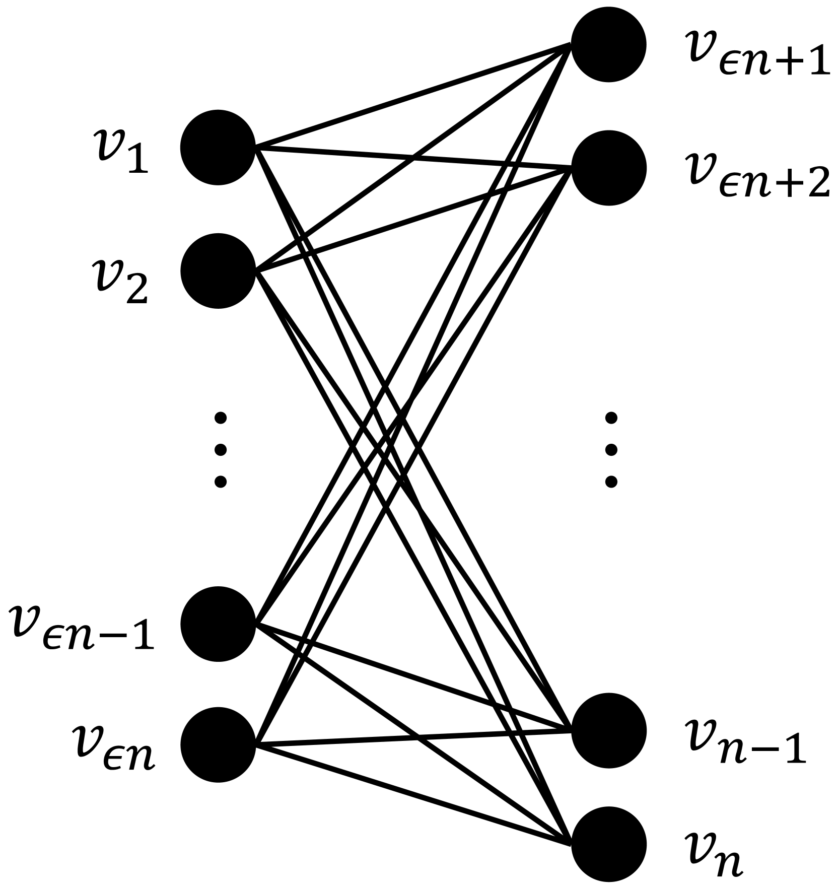
The considered instance of maximum coverage as presented in Example 1 is from Friedrich et al. (2010); Friedrich and Neumann (2015), and can be obtained from the complete bipartite graph in Figure 1(a). The ground set $U$ is given by the set of edges. Each vertex $v_{i}$ corresponds to one subset $S_{i}$ of $U$, which consists of the edges adjacent to the vertex $v_{i}$. The goal is to select at most $k=(1+\delta)n/3$ subsets of $U$ to make the number of contained edges maximal.

Example 1.

The ground set $U$ contains all the edges of the complete bipartite graph in Figure 1(a). Each set $S_{i}$ in $V$ consists of the edges adjacent to the vertex $v_{i}$, i.e., $\forall 1\leq i\leq(1+\delta)n/3$, $S_{i}=\{(v_{i},v_{(1+\delta)n/3+1}),\ldots,(v_{i},v_{n})\}$; $\forall(1+\delta)n/3+1\leq i\leq n$, $S_{i}=\{(v_{i},v_{1}),\ldots,(v_{i},v_{(1+\delta)n/3})\}$, where $(v_{i},v_{j})$ denotes the edge between the vertexes $v_{i}$ and $v_{j}$. The budget $k=(1+\delta)n/3$, and $\delta$ is a small positive constant close to 0.

The two parts of the complete bipartite graph in Figure 1(a) contain $(1+\delta)n/3$ and $(2-\delta)n/3$ vertexes, respectively. As the budget $k=(1+\delta)n/3<(2-\delta)n/3$, the unique optimal solution is $\bm{x}^{*}=1^{(1+\delta)n/3}0^{(2-\delta)n/3}$ (i.e., $\{S_{1},\ldots,S_{(1+\delta)n/3}\}$), which covers all the edges, and has the objective value $f(\bm{x}^{*})=((1+\delta)n/3)\cdot((2-\delta)n/3)=(1+\delta)(2-\delta)n^{2}/9$. We can also observe that if a solution

$$\bm{x}_{\mathrm{local}}\!\in\!\{0^{(1+\delta)n/3}\bm{y}\mid\bm{y}\!\in\!\{0,1\}^{(2-\delta)n/3}\wedge|\bm{y}|\!=\!(1+\delta)n/3\},$$

i.e., contains $(1+\delta)n/3$ sets from $\{S_{(1+\delta)n/3+1},\ldots,S_{n}\}$, it is local optimal, with the objective value $f(\bm{x}_{\mathrm{local}})=((1+\delta)n/3)\cdot((1+\delta)n/3)=(1+\delta)^{2}n^{2}/9$. Adding a set from $\{S_{1},\ldots,S_{(1+\delta)n/3}\}$ into $\bm{x}_{\mathrm{local}}$ will cover $(2-\delta)n/3-(1+\delta)n/3=(1-2\delta)n/3$ more edges. If $i$ sets from $\{S_{1},\ldots,S_{(1+\delta)n/3}\}$ have been added into $\bm{x}_{\mathrm{local}}$, then deleting one set from $\bm{x}_{\mathrm{local}}$ will decrease the number of edges by $(1+\delta)n/3-i$. To make $(1+\delta)n/3-i\leq(1-2\delta)n/3$, $i$ should be at least $\delta n$. Thus, to improve the local optimal solution $\bm{x}_{\mathrm{local}}$, at least $\delta n$ sets from $\{S_{1},\ldots,S_{(1+\delta)n/3}\}$ need to be added into $\bm{x}_{\mathrm{local}}$, and meanwhile at least $\delta n$ sets from $\bm{x}_{\mathrm{local}}$ have to be deleted. The approximation ratio of $\bm{x}_{\mathrm{local}}$ is $f(\bm{x}_{\mathrm{local}})/f(\bm{x}^{*})=(1+\delta)/(2-\delta)$.

(a) $\epsilon=(1+\delta)/3$

(b)

Figure 1: Two complete bipartite graphs.

We prove in Theorem 2 that on the maximum coverage instance in Example 1, $(\mu+1)$-EA requires at least exponential (w.r.t. $n$) expected running time to achieve an approximation ratio larger than $(1+\delta)/(2-\delta)$. The main proof idea is to show that there is some probability that the population of $(\mu+1)$-EA will get trapped in a local optimal solution $\bm{x}_{\mathrm{local}}$, escaping from which requires at least $2\delta n$ bits to be flipped simultaneously.

Theorem 2.

There exists an instance of monotone submodular maximization with a size constraint (more precisely, the maximum coverage instance in Example 1), where the expected running time of $(\mu+1)$-EA with $\mu=n+1$ for achieving an approximation ratio larger than $(1+\delta)/(2-\delta)$ is at least exponential w.r.t. $n$, where $\delta$ is a small positive constant close to 0.

Proof.

In line 1 of Algorithm 2, $(\mu+1)$-EA generates $n+1$ initial solutions randomly, where each solution is sampled from $\{0,1\}^{n}$ uniformly at random. We first consider the event (denoted as $A$) that among the generated $n+1$ initial solutions, one is a local optimal solution $\bm{x}_{\mathrm{local}}$, and the other $n$ solutions do not satisfy the size constraint, i.e., contain more than $k=(1+\delta)n/3$ 1-bits. For a solution $\bm{x}$ randomly sampled from $\{0,1\}^{n}$, the probability of being local optimal is $P(\bm{x}\in\{0^{(1+\delta)n/3}\bm{y}\mid\bm{y}\in\{0,1\}^{(2-\delta)n/3}\wedge|\bm{y}|=(1+\delta)n/3\})=\binom{(2-\delta)n/3}{(1+\delta)n/3}/2^{n}\geq 1/2^{n}$; the probability of having more than $(1+\delta)n/3$ 1-bits is $P(|\bm{x}|>(1+\delta)n/3)=1-P(|\bm{x}|\leq(1+\delta)n/3)=1-P(|\bm{x}|\leq(1-(1-2\delta)/3)\cdot(n/2))\geq 1-e^{-\frac{n}{4}(\frac{1-2\delta}{3})^{2}}$, where the inequality holds by the Chernoff bound. Thus, the event $A$ happens with probability

$$P(A)\geq\frac{n+1}{2^{n}}\cdot\left(1-e^{-\frac{n}{4}(\frac{1-2\delta}{3})^{2}}\right)^{n}=\frac{n+1}{2^{n}}(1-o(1)),$$

where the factor $n+1$ is because $\bm{x}_{\mathrm{local}}$ can be any of the $(n+1)$ initial solutions.

Given the event $A$, we consider that in the first $n$ iterations of $(\mu+1)$-EA, a local optimal solution is always selected from the current population in line 3 of Algorithm 2, and no bits are flipped by the bit-wise mutation operator in line 4. Such an event is denoted as $B$. Because the objective value of a solution which does not satisfy the size constraint is set to $-1$, the copied local optimal solution will replace one solution violating the size constraint in the population after each iteration according to the population updating procedure in lines 5–8 of Algorithm 2. Thus, if the event $B$ happens, the population of $(\mu+1)$-EA will be full of local optimal solutions. Because uniform selection is performed in line 3 of Algorithm 2 and the number of local optimal solutions increases by 1 after each iteration, the event $B$ happens with probability

$$P(B) =\prod^{n}_{i=1}\left(\frac{i}{n+1}\left(1\!-\!\frac{1}{n}\right)^{n}\right)=\frac{n!}{(n\!+\!1)^{n}}\left(1\!-\!\frac{1}{n}\right)^{n^{2}}$$ (8)

$$\geq\sqrt{2\pi n}\left(\frac{n}{e}\right)^{n}\cdot\frac{1}{(n+1)^{n}}\cdot\frac{1}{(2e)^{n}}\geq\frac{\sqrt{2\pi n}}{e(2e^{2})^{n}},$$ (9)

where $i/(n+1)$ is the probability of selecting a local optimal solution from the population in the $i$-th iteration, $(1-1/n)^{n}$ is the probability of keeping all the $n$ bits of the selected solution unchanged in mutation, the first inequality holds by $n!\geq\sqrt{2\pi n}(n/e)^{n}$ due to Stirling’s formula and $(1-1/n)^{n}\geq 1/(2e)$, and the last inequality holds by $(n/(n+1))^{n}=(1-1/(n+1))^{n}\geq 1/e$.

After the events $A$ and $B$ happen, the population consists of $n+1$ local optimal solutions from $\{0^{(1+\delta)n/3}\bm{y}\mid\bm{y}\in\{0,1\}^{(2-\delta)n/3}\wedge|\bm{y}|=(1+\delta)n/3\}$. As we have analyzed before, to improve a local optimal solution $\bm{x}_{\mathrm{local}}$, at least $\delta n$ sets from $\{S_{1},\ldots,S_{(1+\delta)n/3}\}$ need to be added into $\bm{x}_{\mathrm{local}}$, and meanwhile at least $\delta n$ sets from $\bm{x}_{\mathrm{local}}$ have to be deleted. That is, when mutating $\bm{x}_{\mathrm{local}}$, it needs to flip at least $\delta n$ of its $(1+\delta)n/3$ leading 0-bits and at least $\delta n$ of its $(1+\delta)n/3$ 1-bits, the probability of which is at most

$$\binom{(1+\delta)n/3}{\delta n}\cdot\binom{(1+\delta)n/3}{\delta n}\cdot\left(\frac{1}{n}\right)^{2\delta n}$$ (10)

$$\leq\frac{((1+\delta)n/3)^{2\delta n}}{(\delta n)!^{2}}\cdot\!\left(\frac{1}{n}\right)^{2\delta n}\!\!\leq\frac{1}{2\pi\delta n}\cdot\!\left(\frac{e(1+\delta)}{3\delta n}\right)^{2\delta n},$$ (11)

where the last inequality holds by $(\delta n)!\geq\sqrt{2\pi\delta n}(\delta n/e)^{\delta n}$ due to Stirling’s formula. Thus, given the events $A$ and $B$, the expected running time to generate a solution better than $\bm{x}_{\mathrm{local}}$ is at least $2\pi\delta n(3\delta n/(e(1+\delta)))^{2\delta n}$.

Because the approximation ratio of $\bm{x}_{\mathrm{local}}$ is $(1+\delta)/(2-\delta)$, $P(A)\!\geq(n+1)(1-o(1))/2^{n}$ and $P(B)\geq\sqrt{2\pi n}/(e(2e^{2})^{n})$, the expected running time of $(\mu+1)$-EA for achieving an approximation ratio larger than $(1+\delta)/(2-\delta)$ is at least

$$\frac{n+1}{2^{n}}(1-o(1))\cdot\frac{\sqrt{2\pi n}}{e(2e^{2})^{n}}\cdot 2\pi\delta n\left(\frac{3\delta n}{e(1+\delta)}\right)^{2\delta n},$$

which is exponential w.r.t. $n$ because $\delta$ is a small positive constant close to 0. Thus, the theorem holds. ∎

The comparison between Corollary 1 and Theorem 2 clearly shows the advantage of MAP-Elites over $(\mu+1)$-EA. That is, for monotone submodular maximization with a size constraint, MAP-Elites can always achieve the $(1-1/e)$-approximation ratio in expected polynomial time, while there exists an instance where $(\mu+1)$-EA requires at least expected exponential time to achieve an approximation ratio of nearly $1/2$. From the proofs, we can find that MAP-Elites explicitly maintains multiple cells of the behavior space, allowing it to achieve a good solution with $k$ 1-bits by following a path across different cells (i.e., gradually adding the number of 1-bits), while $(\mu+1)$-EA only focuses on the objective value, and may lose diversity in the population and get trapped in local optima (with $k$ 1-bits). This discloses the benefit of simultaneously searching for high-performing solutions at diverse regions in the behavior space, which may provide stepping stones to high-performing solutions in a region that may be difficult to be discovered if searching only in that region.

4 Set Cover

Set cover Feige (1998) as presented in Definition 4 is a well-known NP-hard combinatorial optimization problem. Given a family $V$ of sets (where each set has a corresponding positive weight) that cover a universe $U$ of elements, the goal is to find a subset of $V$ with the minimum weight such that all the elements of $U$ are covered.

Definition 4 (Set Cover).

Given a ground set $U=\{e_{1},e_{2},\ldots,e_{m}\}$, and a collection $V=\{S_{1},S_{2},\ldots,S_{n}\}$ of subsets of $U$ with corresponding weights $w:V\rightarrow\mathbb{R}^{+}$, the goal is to find a subset of $V$ (represented by $\bm{x}\in\{0,1\}^{n}$) such that

$$\mathop{\arg\min}\nolimits_{x\in\{0,1\}^{n}}\;\;\sum\nolimits_{i=1}^{n}w_{i}x_{i}\quad\text{s.t.}\quad\bigcup\nolimits_{i:x_{i}=1}S_{i}=U.$$ (12)

Note that a Boolean vector $\bm{x}\in\{0,1\}^{n}$ represent a subset $X$ of $V$, where the $i$-th bit $x_{i}=1$ if $S_{i}\in X$, and $x_{i}=0$ otherwise. Let $w_{\mathrm{\max}}=\max\{w_{i}\mid 1\leq i\leq n\}$ denote the maximum weight of a single subset $S_{i}$. In the following analysis, we equivalently reformulate the above problem as an unconstrained minimization problem by setting

$$\forall\bm{x}\in\{0,1\}^{n}:f(\bm{x})=w(\bm{x})+\lambda\cdot(m-c(\bm{x})),$$ (13)

where $w(\bm{x})=\sum\nolimits_{i=1}^{n}w_{i}x_{i}$ denotes the weight of $\bm{x}$, $c(\bm{x})=|\bigcup\nolimits_{i:x_{i}=1}S_{i}|$ denotes the number of elements covered by $\bm{x}$, and $\lambda>nw_{\mathrm{\max}}$ is a sufficiently large penalty. That is, a solution covering more elements is better; if covering the same number of elements, a solution with a smaller weight is better.

4.1 Analysis of MAP-Elites

To apply MAP-Elites in Algorithm 1 to solve the set cover problem, we use the number $c(\bm{x})=|\bigcup\nolimits_{i:x_{i}=1}S_{i}|$ of covered elements of a solution $\bm{x}\in\{0,1\}^{n}$ as the behavior descriptor. Thus, the archive $M$ maintained by MAP-Elites contains $m+1$ cells, where for any $0\leq i\leq m$, the $i$-th cell stores the best found solution covering $i$ elements. In each iteration of MAP-Elites, if an offspring solution $\bm{x}^{\prime}$ with $c(\bm{x}^{\prime})=j$ is generated, the $j$-th cell in the archive $M$ will be examined: if the cell is empty or the existing solution in the cell is worse than $\bm{x}^{\prime}$ (i.e., has a larger weight than $\bm{x}^{\prime}$), the $j$-th cell will then be occupied by $\bm{x}^{\prime}$.

We prove in Theorem 3 that after running $O(mn(m+\log n+\log(w_{\max}/w_{\min})))$ expected time, MAP-Elites achieves an approximation ratio of $\ln m+1$, which has been optimal up to a constant factor, unless P$\,=\,$NP Feige (1998). The proof is accomplished by following the behavior of the greedy algorithm Chvatal (1979), inspired from the analysis of GSEMO Friedrich et al. (2010); Qian et al. (2015a). The parameter $I$ of MAP-Elites is set to $m+1$, i.e., it generates $m+1$ initial solutions randomly. As for solving the problem of monotone approximately submodular maximization with a size constraint in the last section, such a setting is for fairness, because the population size $\mu$ of $(\mu+1)$-EA will be set to the number of cells (i.e., $m+1$) contained by the archive $M$.

Theorem 3.

For the set cover problem, the expected running time of MAP-Elites with the parameter $I=m+1$, until finding a solution $\bm{x}$ with $c(\bm{x})=m$ and

$$f(\bm{x})\leq(\ln m+1)\cdot\mathrm{OPT},$$

is $O(mn(m+\log n+\log(w_{\max}/w_{\min})))$, where $m$ is the size of the ground set $U$, $c(\bm{x})=|\bigcup\nolimits_{i:x_{i}=1}S_{i}|$ denotes the number of elements covered by $\bm{x}$, $\mathrm{OPT}$ denotes the optimal function value, and $w_{\max}=\max\{w_{i}\mid 1\leq i\leq n\}$ and $w_{\min}=\min\{w_{i}\mid 1\leq i\leq n\}$ denote the maximum and minimum weights of a single set $S_{i}$, respectively.

Proof.

We divide the optimization process of MAP-Elites into two phases: (1) starts after initialization and finishes after finding the special solution $\bm{0}$ which does not cover any element; (2) starts after phase (1) and finishes after finding a solution with the desired approximation guarantee. Note that the archive $M$ will always contain at most $m+1$ solutions, i.e., $|M|\leq m+1$, because there are $m+1$ cells and the $i$-th cell only stores the best found solution covering $i$ elements.

For phase (1), we consider the minimum weight of solutions in the archive $M$ after running $t$ iterations, denoted as $X_{t}=\min\{w(\bm{x})\mid\bm{x}\in M\}$. Note that $X_{t}=0$ implies that the solution $\bm{0}$ has been found. Then, we are to analyze the expected change of $X_{t}$ after one iteration, denoted as $E(X_{t}-X_{t+1}\mid X_{t})$. Let $\bm{x}$ be a corresponding solution with $w(\bm{x})=X_{t}$. We can observe that $X_{t}$ cannot increase (i.e., $X_{t+1}\leq X_{t}$) because $\bm{x}$ can only be replaced by a solution which covers the same number of elements as $\bm{x}$ (i.e., belongs to the same cell as $\bm{x}$) and has a smaller weight. In the $(t+1)$-th iteration, we consider that $\bm{x}$ is selected in line 7 of Algorithm 1, occurring with probability $1/|M|\geq 1/(m+1)$ due to uniform selection and $|M|\leq m+1$. Then, in line 8, let $\bm{x}^{i}$ denote the solution generated by flipping the $i$-th bit (i.e., $x_{i}$) of $\bm{x}$ and keeping other bits unchanged, which happens with probability $(1/n)(1-1/n)^{n-1}\geq 1/(en)$. If $x_{i}=1$, the generated solution $\bm{x}^{i}$ now has the smallest weight $X_{t}-w_{i}$, and must be included into the archive $M$ (otherwise, the minimum weight of the current solutions has been smaller than $X_{t}$, leading to a contradiction), implying $X_{t+1}=X_{t}-w_{i}$. Thus, we have

$$E(X_{t+1}\mid X_{t})\leq X_{t}-\sum\limits_{i:x_{i}=1}\frac{w_{i}}{en(m+1)}.$$ (14)

Because $X_{t}=w(\bm{x})=\sum\nolimits_{i:x_{i}=1}w_{i}$, we have $E(X_{t}-X_{t+1}\mid X_{t})\geq X_{t}/(en(m+1))$. Furthermore, $X_{0}\leq nw_{\max}$, and the weight of a non-empty solution is at least $w_{\min}=\min\{w_{i}\mid 1\leq i\leq n\}$, i.e., the minimum weight of a single set $S_{i}$. According to the multiplicative drift analysis theorem Doerr et al. (2012), we can derive that the expected running time to make $X_{t}=0$ (i.e., find the solution $\bm{0}$) is at most $en(m+1)(1+\ln(nw_{\max}/w_{\min}))\in O(mn(\log n+\log(w_{\max}/w_{\min})))$.

Let $H_{i}=\sum^{i}_{j=1}1/j$ denote the $i$-th harmonic number, and let $R_{k}=H_{m}-H_{m-k}$. For phase (2), we consider a quantity $K_{\max}$, which is defined as the maximum value of $k$ such that there exists a solution $\bm{x}$ in the archive $M$ with $c(\bm{x})=k$ and $w(\bm{x})\leq R_{k}\cdot\mathrm{OPT}$. Then, we only need to analyze the expected running time until $K_{\max}=m$, implying having found a solution with $c(\bm{x})=m$ (i.e., covering all the elements) and $w(\bm{x})\leq R_{m}\cdot\mathrm{OPT}=H_{m}\cdot\mathrm{OPT}<(\ln m+1)\cdot\mathrm{OPT}$.

After finding the solution $\bm{0}$ with $c(\bm{0})=0$ and $w(\bm{0})=0$, we have $K_{\max}\geq 0$. Assume that currently $K_{\max}=k<m$, and let $\bm{x}$ denote the corresponding solution with $c(\bm{x})=k$ and $w(\bm{x})\leq R_{k}\cdot\mathrm{OPT}$. Because $\bm{x}$ can only be replaced by a solution which covers the same number of elements and has a smaller weight, $K_{\max}$ cannot decrease. Next, we are to show that $K_{\max}$ can increase by flipping a specific 0 bit of $\bm{x}$. Let $\bm{x}^{i}$ denote the solution generated by flipping the $i$-th bit of $\bm{x}$. Let $\delta=\min\{\frac{w_{i}}{c(\bm{x^{i}})-c(\bm{x})}\mid c(\bm{x}^{i})-c(\bm{x})>0\}$, which must satisfy $\delta\leq\mathrm{OPT}/(m-k)$. Otherwise, for any $S_{i}\in\bm{x}^{*}\setminus\bm{x}$, $w_{i}>(c(\bm{x}^{i})-c(\bm{x}))\cdot\mathrm{OPT}/(m-k)$, where $\bm{x}^{*}$ denotes an optimal solution, i.e., $c(\bm{x}^{*})=m$ and $w(\bm{x}^{*})=\mathrm{OPT}$; then, $\sum_{S_{i}\in\bm{x}^{*}\setminus\bm{x}}w_{i}>\big(\sum_{S_{i}\in\bm{x}^{*}\setminus\bm{x}}(c(\bm{x}^{i})-c(\bm{x}))\big)\cdot\mathrm{OPT}/(m-k)$. Because $c(\cdot)$ denotes the number of elements covered by a solution, we have $\sum_{S_{i}\in\bm{x}^{*}\setminus\bm{x}}(c(\bm{x}^{i})-c(\bm{x}))\geq c(\bm{x}^{*})-c(\bm{x})$, and thus $\sum_{S_{i}\in\bm{x}^{*}\setminus\bm{x}}w_{i}>(c(\bm{x}^{*})-c(\bm{x}))\cdot\mathrm{OPT}/(m-k)=\mathrm{OPT}$, where the equality holds by $c(\bm{x}^{*})=m$ and $c(\bm{x})=k$. This contradicts with $\sum_{S_{i}\in\bm{x}^{*}\setminus\bm{x}}w_{i}\leq w(\bm{x}^{*})=\mathrm{OPT}$. Thus, it holds that $\delta\leq\mathrm{OPT}/(m-k)$. By selecting $\bm{x}$ in line 7 of Algorithm 1 and flipping only the 0 bit corresponding to $\delta$ in line 8, MAP-Elites can generate a new offspring solution $\bm{x}^{\prime}$ with $c(\bm{x}^{\prime})=k^{\prime}>k$ and

$$w(\bm{x}^{\prime}) \leq w(\bm{x})+(k^{\prime}-k)\cdot\mathrm{OPT}/(m-k)$$ (15)

$$\leq R_{k}\cdot\mathrm{OPT}+(k^{\prime}-k)\cdot\mathrm{OPT}/(m-k)$$ (16)

$$=\left(\frac{1}{m}+\cdots+\frac{1}{m-k+1}+\frac{k^{\prime}-k}{m-k}\right)\cdot\mathrm{OPT}$$ (17)

$$\leq(1/m+\cdots+1/(m-k^{\prime}+1))\cdot\mathrm{OPT}$$ (18)

$$=(H_{m}-H_{m-k^{\prime}})\cdot\mathrm{OPT}=R_{k^{\prime}}\cdot\mathrm{OPT}.$$ (19)

Once generated, $\bm{x}^{\prime}$ will be included into the archive $M$. Otherwise, there has existed a solution in $M$ which covers $k^{\prime}$ elements and has a weight no larger than $w(\bm{x}^{\prime})$ and thus $R_{k^{\prime}}\cdot\mathrm{OPT}$; this implies that $K_{\max}$ has already been larger than $k$, contradicting with the assumption $K_{\max}=k$. After including $\bm{x}^{\prime}$, $K_{\max}$ increases from $k$ to $k^{\prime}$. Because the probability of selecting $\bm{x}$ and flipping only a specific 0 bit in each iteration of MAP-Elites is at least $(1/|M|)\cdot(1/n)(1-1/n)^{n-1}\geq 1/(en(m+1))$, the expected running time for increasing $K_{\max}$ is at most $en(m+1)$. Since it is sufficient to increase $K_{\max}$ at most $m$ times for making $K_{\max}=m$, the expected running time of phase (2) is $O(m^{2}n)$.

By combining the above two phases, the expected running time of the whole process is $O(mn(\log n+\log(w_{\max}/w_{\min}))+m^{2}n)=O(mn(m+\log n+\log(w_{\max}/w_{\min})))$. Thus, the theorem holds. ∎

4.2 Analysis of $(\mu+1)$-EA

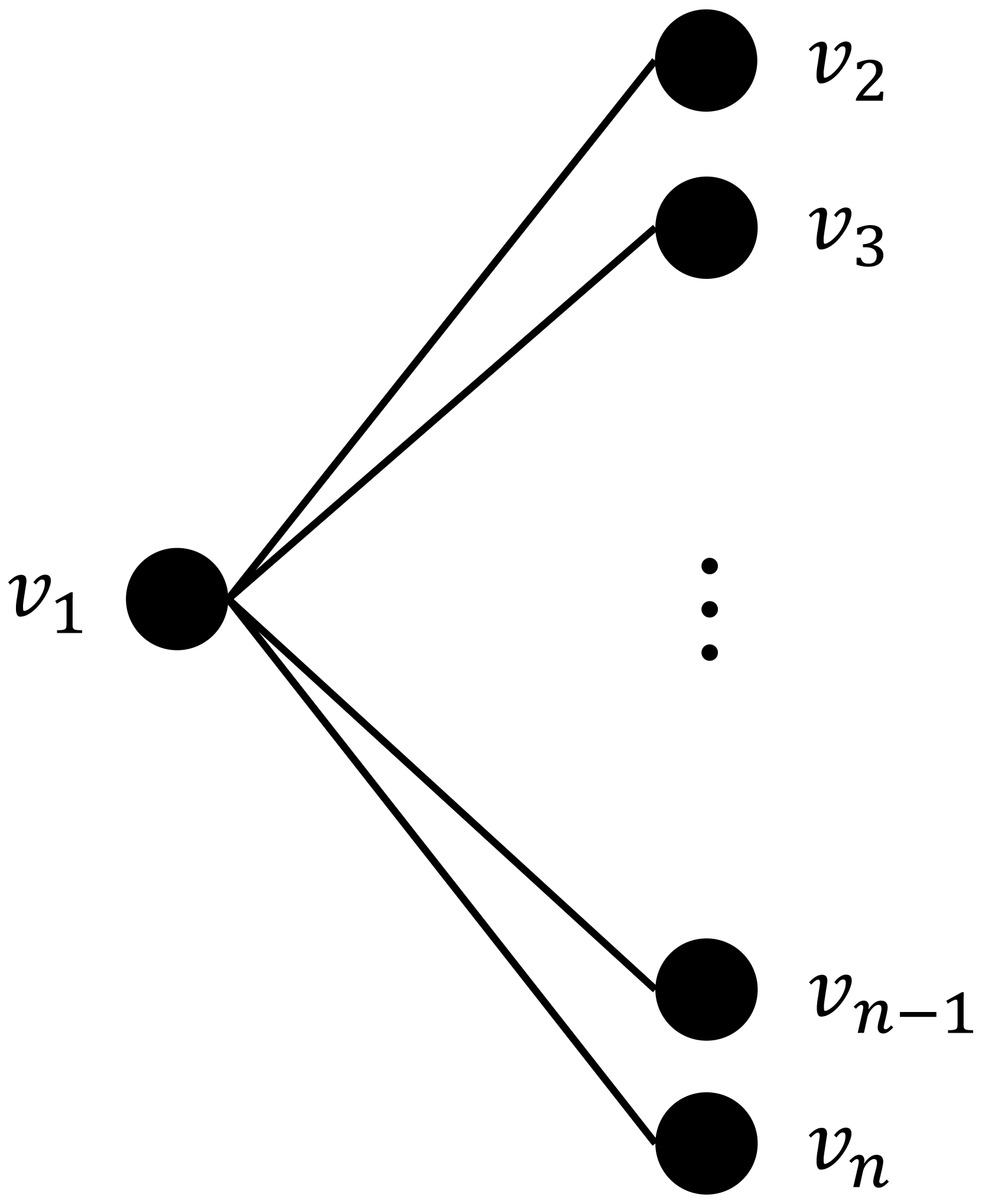
Next, we will give a concrete instance of set cover, where $(\mu+1)$-EA fails to achieve a good approximation ratio in polynomial time. To apply $(\mu+1)$-EA in Algorithm 2 to solve the set cover problem, the population size $\mu$ is set to the number of cells (i.e., $m+1$) contained by the archive $M$ of MAP-Elites for fair comparison. The considered set cover instance is obtained from the complete bipartite graph in Figure 1(b), and presented in Example 2.

Example 2.

The ground set $U$ contains all the $n-1$ edges of the complete bipartite graph in Figure 1(b). Each set $S_{i}$ in $V$ consists of the edges adjacent to the vertex $v_{i}$, i.e., $S_{1}=\{(v_{1},v_{2}),\ldots,(v_{1},v_{n})\}$; $\forall 2\leq i\leq n$, $S_{i}=\{(v_{i},v_{1})\}$, where $(v_{i},v_{j})$ denotes the edge between the vertexes $v_{i}$ and $v_{j}$. Their weights are: $w_{1}=2^{n}$; $\forall 2\leq i\leq n$, $w_{i}=1$.

In this example, the size $m$ of the ground set $U$ is $n-1$, and the maximum and minimum weights of a single set $S_{i}$ are $w_{\max}=2^{n}$, and $w_{\min}=1$, respectively. The unique optimal solution is $\bm{x}^{*}=01^{n-1}$ (i.e., $\{S_{2},\ldots,S_{n}\}$), which covers all the edges, and has the minimum weight $w(\bm{x}^{*})=n-1$. We can also observe that $\bm{x}_{\mathrm{local}}=10^{n-1}$ (i.e., containing only $S_{1}$) is local optimal, with the weight $w(\bm{x}_{\mathrm{local}})=2^{n}$. Furthermore, $\bm{x}_{\mathrm{local}}$ has the smallest weight except $\bm{x}^{*}$, implying that it needs to flip all the $n$ bits to improve $\bm{x}_{\mathrm{local}}$. The approximation ratio of $\bm{x}_{\mathrm{local}}$ is $w(\bm{x}_{\mathrm{local}})/w(\bm{x}^{*})=2^{n}/(n-1)=2^{m+1}/m$. Note that if a solution does not cover all the edges, i.e., does not satisfy the constraint, its objective value will be penalized, as shown by the reformulated equivalent objective function in Eq. (13).

We prove in Theorem 4 that on the set cover instance in Example 2, $(\mu+1)$-EA requires at least exponential (w.r.t. $m$, $n$, and $\log(w_{\max}/w_{\min})$) expected running time to achieve an approximation ratio smaller than $2^{m+1}/m$. The proof idea is similar to that of Theorem 2, i.e., to show that there is some probability that the population of $(\mu+1)$-EA will get trapped in the local optimal solution $\bm{x}_{\mathrm{local}}$, escaping from which requires all the $n$ bits to be flipped simultaneously.

Theorem 4.

There exists an instance of set cover (more precisely, Example 2), where the expected running time of $(\mu+1)$-EA with $\mu=m+1$ for achieving an approximation ratio smaller than $2^{m+1}/m$ is at least exponential w.r.t. $m$, $n$, and $\log(w_{\max}/w_{\min})$.

Proof.

As the population size $\mu=m+1=n$, $(\mu+1)$-EA generates $n$ initial solutions randomly by uniform sampling from $\{0,1\}^{n}$ in line 1 of Algorithm 2. Let $A$ denote the event that one initial solution is the local optimal solution $\bm{x}_{\mathrm{local}}$, and the other $n-1$ initial solutions are all worse than $\bm{x}_{\mathrm{local}}$. Because $\bm{x}_{\mathrm{local}}$ has the best objective value except the optimal solution $\bm{x}^{*}$, the event $A$ happens with probability

$$P(A)=\frac{n}{2^{n}}\cdot\left(1-\frac{2}{2^{n}}\right)^{n-1}=\frac{n}{2^{n}}(1-o(1)),$$

where the factor $n$ is because $\bm{x}_{\mathrm{local}}$ can be any of the $n$ initial solutions. Given the event $A$, we then consider that in the first $n-1$ iterations of $(\mu+1)$-EA, $\bm{x}_{\mathrm{local}}$ is always selected from the current population in line 3 of Algorithm 2, and no bits are flipped by bit-wise mutation in line 4. This event (denoted as $B$) will make the population of $(\mu+1)$-EA consist of $n$ copies of $\bm{x}_{\mathrm{local}}$, because a copy of $\bm{x}_{\mathrm{local}}$ will replace a worse solution in the population after each iteration. The event $B$ happens with probability

$$P(B) =\prod^{n-1}_{i=1}\left(\frac{i}{n}\left(1-\frac{1}{n}\right)^{n}\right)\geq\frac{\sqrt{2\pi(n-1)}}{e(2e^{2})^{n-1}},$$ (20)

where $i/n$ is the probability of selecting $\bm{x}_{\mathrm{local}}$ from the population in the $i$-th iteration (note that the population contains $i$ copies of $\bm{x}_{\mathrm{local}}$ in the $i$-th iteration), $(1-1/n)^{n}$ is the probability of keeping all the $n$ bits of $\bm{x}_{\mathrm{local}}$ unchanged in mutation, and the inequality holds by $(n-1)!\geq\sqrt{2\pi(n-1)}((n-1)/e)^{n-1}$ due to Stirling’s formula, $((n-1)/n)^{n-1}=(1-1/n)^{n-1}\geq 1/e$ and $(1-1/n)^{n}\geq 1/(2e)$.

After the events $A$ and $B$ happen, the population consists of $n$ copies of $\bm{x}_{\mathrm{local}}$. Because $\bm{x}_{\mathrm{local}}=10^{n-1}$ has the best objective value except the optimal solution $\bm{x}^{*}=1^{n-1}0$, it needs to flip all the $n$ bits to make an improvement, the probability of which is $1/n^{n}$. Thus, given the events $A$ and $B$, the expected running time to generate a solution better than $\bm{x}_{\mathrm{local}}$ is $n^{n}$. Because the approximation ratio of $\bm{x}_{\mathrm{local}}$ is $2^{n}/(n-1)$, $P(A)\geq n(1-o(1))/2^{n}$, and $P(B)\geq\sqrt{2\pi(n-1)}/(e(2e^{2})^{n-1})$, the expected running time of $(\mu+1)$-EA for achieving an approximation ratio smaller than $2^{n}/(n-1)$ is at least

$$\frac{n}{2^{n}}(1-o(1))\cdot\frac{\sqrt{2\pi(n-1)}}{e(2e^{2})^{n-1}}\cdot n^{n},$$

which is exponential w.r.t. $n$. In Example 2, we have $m=n-1$ and $\log(w_{\max}/w_{\min})=\log(2^{n}/1)=n$, implying that the theorem holds. ∎

By comparing Theorems 3 and 4, MAP-Elites is clearly superior to $(\mu+1)$-EA for solving the set cover problem. MAP-Elites can always achieve the $(\ln m+1)$-approximation ratio in expected polynomial time, while there exists an instance where $(\mu+1)$-EA requires at least expected exponential time to achieve an approximation ratio smaller than $2^{m+1}/m$. As we have found from the analysis on the problem of monotone submodular maximization with a size constraint in the last section, the simultaneous search for high-performing solutions at diverse regions in the behavior space makes MAP-Elites better. More specifically, MAP-Elites obtains a good solution covering all elements by following a path across different cells of the behavior space (i.e., gradually covering more elements), while $(\mu+1)$-EA may lose diversity in the population and get trapped in local optima in the space of solutions covering all elements.

5 Conclusion and Discussion

This paper continues the line of theoretical studies on QD algorithms which have only just begun. Specifically, it contributes to providing theoretical justification for the benefit of QD algorithms, i.e., bringing better optimization. On the two NP-hard problems, i.e., monotone approximately submodular maximization with a size constraint, and set cover, we prove that MAP-Elites can achieve the (asymptotically) optimal polynomial-time approximation ratio, while $(\mu+1)$-EA requires exponential expected time on some instances. The simultaneous search of QD algorithms for high-performing solutions with diverse behaviors brings better exploration of the search space, helping avoid local optima and find better solutions. In fact, we can find more theoretical evidences by comparing the results from previous separate works on QD and EA’s runtime analysis, though not completely fair. For example, Bossek and Sudholt Bossek and Sudholt (2023) proved that for maximizing any monotone pseudo-Boolean function over $\{0,1\}^{n}$, MAP-Elites that generates one random initial solution and uses the number of 1-bits of a solution as the behavior descriptor can find an optimal solution in $O(n^{2}\log n)$ expected time, while Lengler and Zou Lengler and Zou (2021) proved that $(\mu+1)$-EA with $\mu_{0}\leq\mu\leq n$ (where $\mu_{0}$ is some constant) needs superpolynomial time to optimize some monotone functions. In the future, we will theoretically verify the other benefit of QD algorithms that they can better create a map of high-performing solutions in the behavior space than separately searching for a high-performing solution in each cell of the behavior space, by analyzing the QD-Score metric, i.e., the sum of objective values across all obtained solutions in the archive.

There are many interesting theoretical works to be done, e.g., comparing different QD frameworks (MAP-Elites vs. NSLC), and studying the influence of different components (e.g., parent selection strategies and variation operators) of QD algorithms. The findings may inspire the design of better QD algorithms in practice. Another very interesting work is to study the relationship between MAP-Elites and the corresponding multi-objective EA, GSEMO, as also pointed out in Bossek and Sudholt (2023). By treating the behavior descriptors as the extra objective functions to be optimized, GSEMO behaves somewhat similarly to MAP-Elites. The differences are: 1) MAP-Elites only compares solutions within the same cell (i.e., having the same behavior descriptor values) while GSEMO compares different behavior descriptor values based on the domination relationship; 2) MAP-Elites can control the granularity of the behavior space by setting the number of behavior descriptor values in a cell. The currently known results of MAP-Elites (including Bossek and Sudholt (2023) and ours) match that of GSEMO in Neumann and Wegener (2006); Friedrich et al. (2010); Friedrich and Neumann (2015); Qian et al. (2019). Thus, it would be interesting to show their performance gap on some problems, especially that MAP-Elites may overcome some difficulty of GSEMO due to its good diversity mechanism.

References

- Auger and Doerr [2011] A. Auger and B. Doerr. Theory of Randomized Search Heuristics - Foundations and Recent Developments. World Scientific, Singapore, 2011.
- Bhatt et al. [2022] V. Bhatt, B. Tjanaka, M. C. Fontaine, and S. Nikolaidis. Deep surrogate assisted generation of environments. In Advances in Neural Information Processing Systems 35 (NeurIPS), New Orleans, LA, 2022.
- Bossek and Sudholt [2023] J. Bossek and D. Sudholt. Runtime analysis of quality diversity algorithms. In Proceedings of the 25th ACM Conference on Genetic and Evolutionary Computation (GECCO), pages 1546–1554, Lisbon, Portugal, 2023.
- Chalumeau et al. [2023] F. Chalumeau, R. Boige, B. Lim, V. Macé, M. Allard, A. Flajolet, A. Cully, and T. Pierrot. Neuroevolution is a competitive alternative to reinforcement learning for skill discovery. In Proceedings of the 11th International Conference on Learning Representations (ICLR), Kigali, Rwanda, 2023.
- Chatzilygeroudis et al. [2021] K. Chatzilygeroudis, A. Cully, V. Vassiliades, and J.-B. Mouret. Quality-diversity optimization: A novel branch of stochastic optimization. In Black Box Optimization, Machine Learning, and No-Free Lunch Theorems, pages 109–135. Springer, Cham, Switzerland, 2021.
- Chvatal [1979] V. Chvatal. A greedy heuristic for the set-covering problem. Mathematics of Operations Research, 4(3):233–235, 1979.
- Clune et al. [2013] J. Clune, J.-B. Mouret, and H. Lipson. The evolutionary origins of modularity. Proceedings of the Royal Society B: Biological Sciences, 280(1755):20122863, 2013.
- Colas et al. [2020] C. Colas, V. Madhavan, J. Huizinga, and J. Clune. Scaling MAP-Elites to deep neuroevolution. In Proceedings of the 22th ACM Conference Genetic and Evolutionary Computation (GECCO), pages 67–75, Cancún, Mexico, 2020.
- Conti et al. [2018] E. Conti, V. Madhavan, F. P. Such, J. Lehman, K. O. Stanley, and J. Clune. Improving exploration in evolution strategies for deep reinforcement learning via a population of novelty-seeking agents. In Advances in Neural Information Processing Systems 32 (NeurIPS), pages 5032–5043, Montréal, Canada, 2018.
- Cully and Demiris [2018] A. Cully and Y. Demiris. Quality and diversity optimization: A unifying modular framework. IEEE Transactions on Evolutionary Computation, 22(2):245–259, 2018.
- Cully et al. [2015] A. Cully, J. Clune, D. Tarapore, and J.-B. Mouret. Robots that can adapt like animals. Nature, 521(7553):503–507, 2015.
- Das and Kempe [2011] A. Das and D. Kempe. Submodular meets spectral: Greedy algorithms for subset selection, sparse approximation and dictionary selection. In Proceedings of the 28th International Conference on Machine Learning (ICML), pages 1057–1064, Bellevue, WA, 2011.
- Doerr and Neumann [2020] B. Doerr and F. Neumann. Theory of Evolutionary Computation: Recent Developments in Discrete Optimization. Springer, Cham, Switzerland, 2020.
- Doerr et al. [2012] B. Doerr, D. Johannsen, and C. Winzen. Multiplicative drift analysis. Algorithmica, 64(4):673–697, 2012.
- Doncieux et al. [2019] S. Doncieux, A. Laflaquière, and A. Coninx. Novelty search: A theoretical perspective. In Proceedings of the 21st ACM Conference on Genetic and Evolutionary Computation (GECCO), pages 99–106, Prague, Czech Republic, 2019.
- Ecoffet et al. [2021] A. Ecoffet, J. Huizinga, J. Lehman, K. O. Stanley, and J. Clune. First return, then explore. Nature, 590(7847):580–586, 2021.
- Eysenbach et al. [2018] B. Eysenbach, A. Gupta, J. Ibarz, and S. Levine. Diversity is all you need: Learning skills without a reward function. In Proceedings of the 6th International Conference on Learning Representations (ICLR), Vancouver, Canada, 2018.
- Faldor et al. [2023] M. Faldor, F. Chalumeau, M. Flageat, and A. Cully. MAP-Elites with descriptor-conditioned gradients and archive distillation into a single policy. In Proceedings of the 25th ACM Conference on Genetic and Evolutionary Computation (GECCO), pages 138–146, Lisbon, Portugal, 2023.
- Feige [1998] U. Feige. A threshold of for approximating set cover. Journal of the ACM, 45(4):634–652, 1998.
- Feng et al. [2019] C. Feng, C. Qian, and K. Tang. Unsupervised feature selection by Pareto optimization. In Proceedings of the 33rd AAAI Conference on Artificial Intelligence (AAAI), pages 3534–3541, Honolulu, HI, 2019.
- Fontaine and Nikolaidis [2021] M. C. Fontaine and S. Nikolaidis. Differentiable quality diversity. In Advances in Neural Information Processing Systems 34 (NeurIPS), pages 10040–10052, Virtual, 2021.
- Fontaine et al. [2021] M. C. Fontaine, R. Liu, A. Khalifa, J. Modi, J. Togelius, A. K. Hoover, and S. Nikolaidis. Illuminating Mario scenes in the latent space of a generative adversarial network. In Proceedings of the 35th AAAI Conference on Artificial Intelligence (AAAI), pages 5922–5930, Virtual, 2021.
- Friedrich and Neumann [2015] T. Friedrich and F. Neumann. Maximizing submodular functions under matroid constraints by evolutionary algorithms. Evolutionary Computation, 23(4):543–558, 2015.
- Friedrich et al. [2010] T. Friedrich, J. He, N. Hebbinghaus, F. Neumann, and C. Witt. Approximating covering problems by randomized search heuristics using multi-objective models. Evolutionary Computation, 18(4):617–633, 2010.
- Grillotti and Cully [2022] L. Grillotti and A. Cully. Unsupervised behavior discovery with quality-diversity optimization. IEEE Transactions on Evolutionary Computation, 26(6):1539–1552, 2022.
- Harshaw et al. [2019] C. Harshaw, M. Feldman, J. Ward, and A. Karbasi. Submodular maximization beyond non-negativity: Guarantees, fast algorithms, and applications. In Proceedings of the 36th International Conference on Machine Learning (ICML), pages 2634–2643, Long Beach, CA, 2019.
- Jansen and Wegener [2001] T. Jansen and I. Wegener. On the utility of populations in evolutionary algorithms. In Proceedings of the 3rd ACM Conference on Genetic and Evolutionary Computation (GECCO), pages 1034–1041, San Francisco, CA, 2001.
- Kempe et al. [2003] D. Kempe, J. Kleinberg, and É. Tardos. Maximizing the spread of influence through a social network. In Proceedings of the 9th ACM SIGKDD International Conference on Knowledge Discovery and Data Mining (KDD), pages 137–146, Washington, DC, 2003.
- Krause et al. [2008] A. Krause, A. Singh, and C. Guestrin. Near-optimal sensor placements in Gaussian processes: Theory, efficient algorithms and empirical studies. Journal of Machine Learning Research, 9:235–284, 2008.
- Kumar et al. [2020] S. Kumar, A. Kumar, S. Levine, and C. Finn. One solution is not all you need: Few-shot extrapolation via structured MaxEnt RL. In Advances in Neural Information Processing Systems 34 (NeurIPS), pages 8198–8210, Virtual, 2020.
- Lehman and Stanley [2011a] J. Lehman and K. O. Stanley. Abandoning objectives: Evolution through the search for novelty alone. Evolutionary Computation, 19(2):189–223, 2011.
- Lehman and Stanley [2011b] J. Lehman and K. O. Stanley. Evolving a diversity of virtual creatures through novelty search and local competition. In Proceedings of the 13th ACM Conference on Genetic and Evolutionary Computation (GECCO), pages 211–218, Dublin, Ireland, 2011.
- Lengler and Zou [2021] J. Lengler and X. Zou. Exponential slowdown for larger populations: The (+1)-EA on monotone functions. Theoretical Computer Science, 875:28–51, 2021.
- Lim et al. [2022] B. Lim, M. C. Flageat, and A. Cully. Efficient exploration using model-based quality-diversity with gradients. arXiv:2211.12610, 2022.
- Liu et al. [2023] D.-X. Liu, X. Mu, and C. Qian. Human assisted learning by evolutionary multi-objective optimization. In Proceedings of the 37th AAAI Conference on Artificial Intelligence (AAAI), pages 12453–12461, Washington, DC, 2023.
- Lupu et al. [2021] A. Lupu, H. Hu, and J. Foerster. Trajectory diversity for zero-shot coordination. In Proceedings of the 38th International Conference on Machine Learning (ICML), pages 7204–7213, Virtual, 2021.
- Mouret and Clune [2015] J.-B. Mouret and J. Clune. Illuminating search spaces by mapping elites. arXiv:1504.04909, 2015.
- Nemhauser et al. [1978] G. L. Nemhauser, L. A. Wolsey, and M. L. Fisher. An analysis of approximations for maximizing submodular set functions – I. Mathematical Programming, 14(1):265–294, 1978.
- Neumann and Wegener [2006] F. Neumann and I. Wegener. Minimum spanning trees made easier via multi-objective optimization. Natural Computing, 3(5):305–319, 2006.
- Neumann and Witt [2010] F. Neumann and C. Witt. Bioinspired Computation in Combinatorial Optimization - Algorithms and Their Computational Complexity. Springer, Berlin, Germany, 2010.
- Nikfarjam et al. [2022a] A. Nikfarjam, A. Neumann, and F. Neumann. On the use of quality diversity algorithms for the traveling thief problem. In Proceedings of the 24th ACM Conference on Genetic and Evolutionary Computation (GECCO), pages 260–268, Boston, MA, 2022.
- Nikfarjam et al. [2022b] A. Nikfarjam, A. Viet Do, and F. Neumann. Analysis of quality diversity algorithms for the knapsack problem. In Proceedings of the 17th International Conference on Parallel Problem Solving from Nature (PPSN), pages 413–427, Dortmund, Germany, 2022.
- Nilsson and Cully [2021] O. Nilsson and A. Cully. Policy gradient assisted MAP-Elites. In Proceedings of the 23rd ACM Conference on Genetic and Evolutionary Computation (GECCO), page 866–875, Lille, France, 2021.
- Parker-Holder et al. [2020] J. Parker-Holder, A. Pacchiano, K. M. Choromanski, and S. J. Roberts. Effective diversity in population based reinforcement learning. In Advances in Neural Information Processing Systems 34 (NeurIPS), pages 18050–18062, Virtual, 2020.
- Pierrot et al. [2022] T. Pierrot, V. Macé, F. Chalumeau, A. Flajolet, G. Cideron, K. Beguir, A. Cully, O. Sigaud, and N. Perrin-Gilbert. Diversity policy gradient for sample efficient quality-diversity optimization. In Proceedings of the 24th ACM Conference on Genetic and Evolutionary Computation (GECCO), pages 1075–1083, Boston, MA, 2022.
- Pugh et al. [2016] J. K. Pugh, L. B. Soros, and K. O. Stanley. Quality diversity: A new frontier for evolutionary computation. Frontiers Robotics AI, 3:40, 2016.
- Qian et al. [2015a] C. Qian, Y. Yu, and Z.-H. Zhou. On constrained Boolean Pareto optimization. In Proceedings of the 24th International Joint Conference on Artificial Intelligence (IJCAI), pages 389–395, Buenos Aires, Argentina, 2015.
- Qian et al. [2015b] C. Qian, Y. Yu, and Z.-H. Zhou. Subset selection by Pareto optimization. In Advances in Neural Information Processing Systems 28 (NeurIPS), pages 1765–1773, Montreal, Canada, 2015.
- Qian et al. [2016] C. Qian, J.-C. Shi, Y. Yu, K. Tang, and Z.-H. Zhou. Parallel Pareto optimization for subset selection. In Proceedings of the 25th International Joint Conference on Artificial Intelligence (IJCAI), pages 1939–1945, New York, NY, 2016.
- Qian et al. [2018] C. Qian, Y. Yu, and K. Tang. Approximation guarantees of stochastic greedy algorithms for subset selection. In Proceedings of the 27th International Joint Conference on Artificial Intelligence (IJCAI), pages 1478–1484, Stockholm, Sweden, 2018.
- Qian et al. [2019] C. Qian, Y. Yu, K. Tang, X. Yao, and Z.-H. Zhou. Maximizing submodular or monotone approximately submodular functions by multi-objective evolutionary algorithms. Artificial Intelligence, 275:279–294, 2019.
- Qian et al. [2021] C. Qian, C. Bian, Y. Yu, K. Tang, and X. Yao. Analysis of noisy evolutionary optimization when sampling fails. Algorithmica, 83(4):940–975, 2021.
- Salehi et al. [2022] A. Salehi, A. Coninx, and S. Doncieux. Few-shot quality-diversity optimization. IEEE Robotics and Automation Letters, 7(2):4424–4431, 2022.
- Sfikas et al. [2021] K. Sfikas, A. Liapis, and G. N. Yannakakis. Monte Carlo elites: Quality-diversity selection as a multi-armed bandit problem. In Proceedings of the 23rd ACM Conference on Genetic and Evolutionary Computation (GECCO), pages 180–188, Lille, France, 2021.
- Storch [2008] T. Storch. On the choice of the parent population size. Evolutionary Computation, 16(4):557–578, 2008.
- Strouse et al. [2021] DJ Strouse, K. McKee, M. Botvinick, E. Hughes, and R. Everett. Collaborating with humans without human data. In Advances in Neural Information Processing Systems 34 (NeurIPS), pages 14502–14515, Virtual, 2021.
- Tjanaka et al. [2022] B. Tjanaka, M. C. Fontaine, J. Togelius, and S. Nikolaidis. Approximating gradients for differentiable quality diversity in reinforcement learning. In Proceedings of the 24th ACM Conference on Genetic and Evolutionary Computation (GECCO), page 1102–1111, Boston, MA, 2022.
- Vassiliades et al. [2018] V. Vassiliades, K. I. Chatzilygeroudis, and J.-B. Mouret. Using centroidal voronoi tessellations to scale up the multidimensional archive of phenotypic elites algorithm. IEEE Transactions on Evolutionary Computation, 22(4):623–630, 2018.
- Wang et al. [2022] Y. Wang, K. Xue, and C. Qian. Evolutionary diversity optimization with clustering-based selection for reinforcement learning. In Proceedings of the 10th International Conference on Learning Representations (ICLR), Virtual, 2022.
- Wang et al. [2023] R.-J. Wang, K. Xue, H. Shang, C. Qian, H. Fu, and Q. Fu. Multi-objective optimization-based selection for quality-diversity by non-surrounded-dominated sorting. In Proceedings of the 32nd International Joint Conference on Artificial Intelligence (IJCAI), pages 4335–4343, Macao, SAR, China, 2023.
- Wang et al. [2024] R.-J. Wang, K. Xue, C. Guan, and C. Qian. Quality-diversity with limited resources. In Proceedings of the 41st International Conference on Machine Learning (ICML), Vienna, Austria, 2024.
- Wiegand [2023] R. P. Wiegand. Preliminary analysis of simple novelty search. Evolutionary Computation, pages 1–25, 2023.
- Witt [2006] C. Witt. Runtime analysis of the (+1) EA on simple pseudo-Boolean functions. Evolutionary Computation, 14(1):65–86, 2006.
- Xue et al. [2024] K. Xue, R.-J. Wang, P. Li, D. Li, J. Hao, and C. Qian. Sample-efficient quality-diversity by cooperative coevolution. In Proceedings of the 12th International Conference on Learning Representations (ICLR), Vienna, Austria, 2024.
- Yuan et al. [2023] L. Yuan, Z. Zhang, K. Xue, H. Yin, F. Chen, C. Guan, L. Li, C. Qian, and Y. Yu. Robust multi-agent coordination via evolutionary generation of auxiliary adversarial attackers. In Proceedings of the 37th AAAI Conference on Artificial Intelligence (AAAI), pages 11753–11762, Washington, DC, 2023.
- Zhang et al. [2023] Y. Zhang, M. C. Fontaine, V. Bhatt, S. Nikolaidis, and J. Li. Multi-robot coordination and layout design for automated warehousing. In Proceedings of the 32nd International Joint Conference on Artificial Intelligence (IJCAI), pages 5503–5511, Macao, SAR, China, 2023.
- Zhou et al. [2019] Z.-H. Zhou, Y. Yu, and C. Qian. Evolutionary Learning: Advances in Theories and Algorithms. Springer, Singapore, 2019.