CodeComplex: Dataset for Worst-Case Time Complexity Prediction

Abstract

Reasoning ability of Large Language Models (LLMs) is a crucial ability, especially in complex decision-making tasks. One significant task to show LLMs’ reasoning capability is code time complexity prediction, which involves various intricate factors such as the input range of variables and conditional loops. Current benchmarks fall short of providing a rigorous assessment due to limited data, language constraints, and insufficient labeling. They do not consider time complexity based on input representation and merely evaluate whether predictions fall into the same class, lacking a measure of how close incorrect predictions are to the correct ones. To address these dependencies, we introduce CodeComplex, the first robust and extensive dataset designed to evaluate LLMs’ reasoning abilities in predicting code time complexity. CodeComplex comprises 4,900 Java codes and an equivalent number of Python codes, overcoming language and labeling constraints, carefully annotated with complexity labels based on input characteristics by a panel of algorithmic experts. Additionally, we propose specialized evaluation metrics for the reasoning of complexity prediction tasks, offering a more precise and reliable assessment of LLMs’ reasoning capabilities. We release our dataset and baseline models publicly to encourage the relevant (NLP, SE, and PL) communities to utilize and participate in this research.

1 Introduction

Large Language Models (LLMs) demonstrate significant potential in complex decision-making tasks, with their inference capabilities being particularly valuable in software development Austin et al. (2021); Jain et al. (2021). To further test LLM’s inferencing abilities, we showcase this domain of predicting the code time complexity, which requires the consideration of numerous intricate factors. For example, factors such as algorithmic structure Turing (1936); Bentley et al. (1980), data input size, and resource constraints can all influence the time complexity of code Nogueira (2012); Hutter et al. (2014). Understanding and optimizing these factors is crucial for improving the performance of complex algorithms and generating efficient code Peng et al. (2021); Lu et al. (2021).

Despite the existence of benchmarks for the time complexity analysis, such as CoRCoD Sikka et al. (2020), and TASTY Moudgalya et al. (2023), these benchmarks have limitations on their current state. Notably, CoRCoD is the only publicly available dataset that is small in size, and while TASTY considers both time and space complexity, its dataset remains undisclosed. Consequently, there is a clear need for a comprehensive and publicly accessible benchmark that addresses these shortcomings.

Our work aims to fill this gap by introducing CodeComplex, a dataset designed to be the definitive benchmark for evaluating LLMs’ time complexity inference abilities. CodeComplex offers several distinct advantages over existing benchmarks. Firstly, it provides a larger and more diverse dataset, encompassing a broad range of programming languages beyond the limited scope of CoRCoD, which focuses solely on Java. Secondly, our dataset encompasses a more comprehensive set of labeled complexity classes that cover general-use problem-solving algorithms, enabling a more detailed analysis. Thirdly, CodeComplex considers the representation of input data, distinguishing between numeric values and input size indicators, which is critical for accurate complexity analysis. Lastly, we suggest detailed metrics that allow for a more nuanced assessment of LLMs’ performance, moving beyond simple class-based evaluations.

In summary, our contributions are as follows:

1. Comprehensive Dataset: We present a novel dataset with a comprehensive range of algorithmic problems that includes bilingual programming languages, offering a significant expansion upon existing benchmarks.

2. Detailed Complexity Analysis: We annotate the code complexity through complexity analysis of the representation of input data, distinguishing between numeric interpretations and input size indicators.

3. Robustness of Evaluation Metrics: We implement precise evaluation metrics for a rigorous and nuanced assessment of LLMs’ time complexity inference, facilitating accurate comparisons with state-of-the-art baselines.

Through these contributions, CodeComplex aims to advance the study of LLMs inference capabilities with the task of predicting code time complexity, ultimately fostering the development of optimized software. Our benchmark sets a new standard for the evaluation of LLMs, providing a robust and comprehensive tool for researchers and practitioners alike.

Figure 1: Overview of the CodeComplex dataset creation process.

2 Related Work

The LLMs have led to numerous advances in the field of natural language processing Brown et al. (2020); Chowdhery et al. (2023). Therefore, recent research is ongoing to improve the reasoning ability of LLMs. Numerous prompt engineering techniques emerged, such as zero-shot, few-shot, chain of thought, and prompt changing Wei et al. (2022); Wang et al. (2023); Yao et al. (2023). Specifically, the chain of thought prompting was proposed to encourage them to engage in inferential thinking, with the subsequent application of arithmetic, commonsense, and sentiment reasoning. The methodologies demonstrated that when the LLMs’ reasoning was improved, their capability to perform a range of tasks was enhanced.

Nevertheless, it is evident that LLMs are still constrained in their capacity to reason about complex tasks. The enhancement of LLM’s capacity to reason effectively in complex domains is highly dependent upon the availability of a domain-specific and sophisticated dataset. In the field of code time complexity, some representative complex tasks have been proposed as a method for improving the reasoning ability of LLM models. Recently, Sikka et al. (2020) explored code complexity prediction using machine learning-based methods. They curated the CoRCoD dataset comprising 929 annotated Java codes. These codes were enriched with various hand-engineered features extracted from the code, encompassing counts of loops, methods, variables, jumps, breaks, switches, and the identification of specific data structures or algorithms like priority queues, hash maps, hash sets, and sorting functions. Employing machine learning classification algorithms such as $K$-means, random forest, decision tree, SVM, and more, they made predictions based on these diverse features. Additionally, they explored graph2vec Narayanan et al. (2017), a neural graph embedding framework that operates on a program’s AST and achieves comparable performance results.

Another exploration by Prenner and Robbes (2021) scrutinized the potential of pre-trained programming language understanding models, particularly CodeBERT Feng et al. (2020), for predicting code complexity. Their experiments showcased promising results, suggesting that pre-trained models could serve as a viable solution in this domain. In the most recent development, Moudgalya et al. (2023) tackled the analysis of time and space complexity using language models. They leveraged codes sourced from GeeksForGeeks and CoRCoD, alongside a dataset comprising 3,803 Java codes. Their work showcased the viability of fine-tuning pre-trained language models such as GraphCodeBERT Guo et al. (2021) for predicting both time and space complexity, thereby opening new avenues for exploration in this field.

3 The CodeComplex Dataset

The CodeComplex dataset contains a collection of codes written in two languages, Java and Python, from a competitive programming platform. Our dataset originates from Codeforces and collects data from CodeContests Li et al. (2022), a competitive programming dataset tailored for machine learning applications created by DeepMind. It comprises 9,800 codes, evenly split between Java and Python, with 4,900 codes each. We have categorized these codes into seven distinct complexity classes: constant ($O(1)$), linear ($O(n)$), quadratic ($O(n^{2})$), cubic ($O(n^{3})$), logarithmic ($O(\ln n)$, $O(n\ln n)$), and exponential. Each class contains a minimum of 500 Java and Python codes.

We annotated all 9,800 codes with experts, which include the 317 Java codes in the CoRCoD dataset from Codeforces. It is worth mentioning that the CoRCoD, a previous dataset used for code complexity prediction, categorizes Java codes into five complexity classes: $O(1)$, $O(n)$, $O(n^{2})$, $O(\ln n)$, and $O(n\ln n)$. However, it suffers from imbalanced class distribution, evident in Table 1, with a relatively small size of 929 Java code samples in total. Our expansion significantly enhances the dataset’s value for research, particularly concerning DL-based models outlined in Section 4.

Class	CoRCoD	CodeComplex
	Java	Java	Python
${O(1)}$	143	750 (+ 62)	791
${O(n)}$	382	779 (+ 117)	853
${O(n^{2})}$	200	765 (+ 48)	657
${O(n^{3})}$	0	601	606
${O(\ln n)}$	54	700 (+ 18)	669
${O(n\ln n)}$	150	700 (+ 72)	796
exponential	0	605	528
Total	929	4,900 (+ 317)	4,900

Table 1: Statistical difference between CoRCoD and CodeComplex. Numbers in parentheses imply the number of codes from CoRCoD.

3.1 Data Collection

The original corpus of code is from CodeContests, which collected 128 million codes from Codeforces. The corpus only contained information about the contest ID, problem, username, language, acceptance, and statistics (runtime and memory). We extracted the selected problems from this corpus and identified each code’s complexity.

Code samples were selected within the matching candidates with the following conditions. First, we checked the relevance of the problem. There are many problems within a coding competition, but not all of them fall into the scope of complexities we seek to compromise. Therefore, the problems were first analyzed to check whether or not they were in the complexity class of our dataset. If the problem was determined to be in one of the seven complexity classes, then we marked the problem as a candidate for the dataset. This helps to establish a clear base dataset for the complexity domain. Second, we checked the completeness and correctness of the code. We filtered codes that are available to pass the given problem in the contest, meaning that the code is functional, self-contained, and correct on the given task. One of the reasons for using code competition data is that we can check if the code is correct for the problem. Lastly, we wanted a large pool of code samples for a given problem. We took code samples from problems with abundant submissions. This helped to clarify the problem’s robustness and variation.

Consider the following Python program that solves a problem with $O(1)$ time complexity:

⬇

hand = buf.split()

t = []

for i in range(3):

t.append([])

for j in range(9):

t[i].append(0)

for x in hand:

idx = 0

# Following lines are omitted.

Despite the short length of the code, it is not trivial to understand that the time complexity of the above code is actually constant, which implies that the number of instructions for executing the program does not depend on the input size. In fact, the problem description says that the input always consists of three strings separated by whitespace and, therefore, the size of the list hand is actually constant. Hence, it is impossible to correctly calculate the time complexity of a code only by analyzing the code, as the problem description sometimes has a big hint to determine the time complexity.

3.2 Data Preprocessing

Data preprocessing is an important step in preparing datasets for analysis or machine learning tasks. In this process, we utilize dead code elimination and comment removal. Dead code elimination involves removing any code that does not contribute to the functionality or output of the program, thereby reducing unnecessary clutter. From each code, we marked irrelevant codes and unreachable codes as dead codes. Irrelevant code involves variables, functions, and classes that were never used or never called, and unreachable code involves conditional statements that cannot be satisfied and statements that cannot be reached because of control statements such as continue and return.

On the other hand, comment removal entails stripping out any comments within the codebase, which are meant for human understanding. We removed the comments since the fragments could be exploited by the models to improve the accuracy of predicting the time complexity of models.

3.3 Annotation Process

Our primary objective is to create a solid foundation for accurately classifying time complexities. To achieve this, we have meticulously designed a procedure to generate a robust dataset with minimal noise and high quality. We specifically filter ‘correct’ Java and Python codes, ensuring they pass all test cases, including hidden ones. These codes form the basis of our statistical population. Categorizing problems based on problem-solving strategies involves leveraging annotations from CodeContests. Each problem in the dataset is associated with a plausible problem-solving strategy, such as brute force, dynamic programming, or backtracking, as outlined in CodeContests. Following this initial categorization, a detailed analysis of each problem is conducted. This analysis considers input and output variables, utilized data structures, and the overall workflow of the code. Subsequently, the code for each problem is annotated based on its specific input characteristics. More precisely, we take the largest input variable as the main factor in calculating the overall time complexity. By analyzing the code, we consider each control sequence on the code to determine if the input impacts a control segment or is constant. Note that we assume a unit-cost RAM model that requires the same cost for accessing all memory locations for calculating the time complexity. Our core annotation process adheres to four key rules:

1. Consider the input size and the output size as parameters to determine time complexity, with measurement based on the largest parameter among the input variables.

2. Account the impact of used packages and libraries, such as hashmap, sorting, and string-matching algorithms, on time complexity.

3. Treating each test case within a single input separately for complexity measurement.

4. Classifying cases with fixed constants as having a constant time complexity.

The annotation was held by three annotators who have expertise in the algorithm. In the initial annotation step, each annotator annotated each problem independently. Each reasoned on how we judged the input and annotated the time complexity.

Figure 2: Statistics of CodeComplex dataset. The first and second lines are for Java and Python codes, respectively.

During the agreement process, the annotators collaborated closely to reconcile any discrepancies in their annotations. We engaged in thorough discussions, sharing our reasoning and insights to reach a consensus on the appropriate time complexity classification for each problem. In cases where disagreements arose, the annotators carefully evaluated the evidence and considered alternative perspectives before arriving at a mutually acceptable classification. The involvement of ChatGPT serves as a neutral advisor to validate the annotations and offer additional perspectives on complex cases. Through open communication and collaborative decision-making, the annotators ensure the accuracy and reliability of the final dataset. However, it is essential to note the significant impact of input formats and constraints on the actual time complexity of algorithmic problems. These constraints often lead to deviations from the ideal time complexity. Think of a scenario in which the input exploits the problem constraints in time complexity. Despite the problem of having a quadratic time complexity, the provided input constraints may result in linear running time. Moreover, determining the parameter for complexity measurement becomes crucial when faced with multiple input parameters. Additionally, certain code submissions optimize execution based on problem constraints, thus influencing code complexity assessment.

	TASTY	CODAIT	CoRCoD	CodeComplex
Languages	O	X	X	O
Accessibility	X	X	O	O
Sufficient Labels	O	$\bigtriangleup$	$\bigtriangleup$	O
Input-based Annotation	X	X	X	O

Table 2: Comparison between CodeComplex and other time complexity prediction datasets.

The CodeComplex dataset offers a meticulously curated collection of algorithmic problems and corresponding Java and Python code submissions. It serves as a foundation for accurately classifying time complexities and problem-solving strategies. Figure 2 demonstrates basic statistics of the codes for the number of lines, functions, variables, depth of code (DoC), and depth of iterations (DoI). Moreover, both Java and Python solutions displayed comparable characteristics when considering the depth of iterations, reflecting nested loops. However, a distinctive trait of Python code was its abundance of variables, potentially attributed to Python’s lack of explicit variable declaration requirements. This inherent difference in variable declaration mechanisms might contribute to the observed discrepancy in variable counts between the two languages within our dataset. Table 2 summarizes the strengths of our dataset.

3.4 Dataset Overview

Various Data

We have collected the dataset to include multiple problems upon various algorithm categories. Each complexity class includes problems from dynamic programming, brute force, dynamic programming, divide and conquer, and much more. The dataset provides the problem tags from Codeforces, which the user can use to verify the algorithm categories. Also, we can see in Figure 2, that our dataset is not biased in the number of functions or variables for a given complexity class. The traditional models in Table 3 fail to verify the complexity class from these features, which further shows that the solution codes have an even distribution among the complexity classes.

Balanced Complexity Classes

One of the significant strengths of our dataset is the careful balancing of complexity classes. Balanced classes prevent bias in the reasoning process of LLMs and enable more accurate and generalized model performance by providing a comprehensive learning experience across all possible scenarios. However, in Tables 1, the CoRCoD dataset exhibits imbalances among the classes. In contrast, our dataset provides balanced class data, ensuring an accurate and reliable prediction result of LLM models.

Open Access

In previous research on benchmarking the time complexity of code, it was observed that open data sources for code complexity prediction are notably scarce, with CoRCoD being one of the few available datasets. In contrast, our dataset is an open-source resource, providing an accessible and practical solution for researchers and practitioners in the field.

Fully Human Generated and Annotated Dataset

The Codecomplex dataset is labeled manually by three human annotators and all final decisions and verifications are made by humans. Also, the source codes are collected from the codes before LLMs became present, which makes them free of machine-generated codes.

Thorough Validation

During the process of code complexity annotation, a thorough validation was conducted. Three annotators annotated using structured guidelines and cross-validated each other’s annotations and the reasoning process. Also, we used ChatGPT as a failsafe precaution to validate the labels. If the response from ChatGPT disagrees, the annotators re-evaluated the code through edge case validation.

4 Experiments

As a preliminary study on code complexity prediction using a large-scale dataset, we conduct experiments with well-known machine learning-based solutions and large language models(LLMs). First, we try to replicate the result by Sikka et al. (2020) by employing traditional models such as decision tree (DT), random forest (RF), and support vector machine (SVM). Second, we use pre-trained programming language models (PLMs) such as CodeBERT Feng et al. (2020), GraphCodeBERT Guo et al. (2021), UniXcoder Guo et al. (2022), PLBART Ahmad et al. (2021), CodeT5 Wang et al. (2021), and CodeT5+ Wang et al. (2021). Note that we can further categorize these models into two groups where the first group (CodeBERT, GraphCodeBERT, and UniXcoder) only uses encoder architecture, and the second group (PLBART, CodeT5, and CodeT5+) exploits encoder-decoder architecture. Finally, we test the dataset on closed-source LLMs, ChatGPT3.5, ChatGPT4.0 OpenAI (2024), Gemini Pro Google (2024), and test open source LLMs Llama Touvron et al. (2023), CodeGemma, Gemma1 and Gemma2 Team et al. (2024), Mistral-Nemo Jiang et al. (2023), Qwen2 and Qwen2.5 Yang et al. (2024) from an instruction-tuned and a fine-tuned version of our dataset.

4.1 Experimental Settings

We divide the CodeComplex into training and test datasets by a 9 to 1 ratio for both Java and Python. As a result, the training and test datasets comprise 8,820 and 980 codes, respectively. Hyperparameters and methods to fine-tune each model can be found in section B.

4.2 Evaluation Metric

Hierarchy Complexity Score(HC-Score)

There are multiple approaches for estimating complex reasoning capabilities of LLMs. To maximize the effectiveness of our dataset, we propose a novel evaluation metric, the Hierarchy Complexity Score (HC-Score). Unlike traditional accuracy measures, the HC-Score incorporates considerations of the code-time-complexity hierarchy, penalizing predictions in proportion to their deviation from the correct answer. Our evaluation metric HC-Score is computed as follows:

$$\mathrm{HC\text{-}Score}(P,R)=\frac{\sum_{i=1}^{N}\frac{|p_{i}-r_{i}|}{\text{Number of class}}}{N},$$

where we have $N$ number of $p_{i}\in P$ and $r_{i}\in R$ where $p_{i}$ is a prediction and $r_{i}$ is an answer. Also, we can expand this metric by reducing the scoring window of a single class as follows:

$$\mathrm{HC\text{-}Score}_{w}(P,R)=\frac{\sum_{i=1}^{N}max(1-\frac{|p_{i}-r_{i}|}{w},0)}{N},$$

where $w$ is the size of the window for each class. Predictions that closely approximate the correct result incur minimal penalties, while those with substantial errors are penalized more heavily. This nuanced scoring system aims to provide a more precise assessment of an LLM’s reasoning abilities by accounting for the complexity of the tasks at hand. Our contribution is the introduction of this refined evaluation metric, which offers a discriminative and comprehensive tool for assessing model performance. The HC-Scored metric facilitates a deeper understanding of LLM capabilities, guiding further advancements in the development of sophisticated language models.

5 Results & Analysis

We present some selected interesting experimental results and analysis for various scenarios in the following Section. Full experimental results can be found in the Appendix C due to the lack of space.

5.1 Comparison of Java and Python

Java and Python are both popular programming languages, each with its unique features and characteristics that influence code structures and development practices. One key difference between Java and Python is the syntax typing. Java has to declare variables with their data types beforehand, but Python variables can be assigned without explicit type declarations.

Model	Java			Python
	F1	HC	HC2	F1	HC	HC2
Decision Tree	44.4	82.3	56.1	37.3	79.9	50.9
Random Forest	41.9	80.0	51.9	40.0	80.3	52.6
SVM	24.3	71.9	39.1	17.2	66.8	36.0
CodeBERT	77.3	90.9	80.2	73.3	88.7	76.5
GraphCodeBERT	85.5	94.1	87.4	80.8	92.2	83.5
UniXcoder	86.5	94.6	88.2	85.4	94.0	87.4
PLBART	85.3	94.3	87.1	77.2	91.0	80.7
CodeT5	82.4	93.1	84.8	75.5	89.9	79.1
CodeT5+	85.8	94.6	88.0	78.2	91.0	81.2
Gemini Pro	29.7	80.1	48.6	33.4	80.2	51.8
ChatGPT 3.5	52.9	87.0	66.2	44.2	83.4	59.9
ChatGPT 4.0	60.6	90.0	72.7	52.7	87.2	67.4

Table 3: Performance comparison between Java and Python. Macro F1 score and HC scores are displayed.

UniXcoder was the best of the listed modes, and even the wrong answers lie in a similar class which is hard to distinguish. The HC scoring metric always boosts the score since it grants some score to wrong predictions. However, we can see by the HC score that LLMs are more affected than the traditional and program language models. Since LLMs try to reason parts of the codes and combine those results into a whole answer, LLMs tend to land closer to the correct answer if the parts are analyzed correctly.

5.2 Effect of Code Length

Intuitively, it is natural to assume that the shorter the code is, the easier it is to predict the complexity. To confirm our assumption, we categorize codes into four groups according to the number of tokens of the codes. If a code has less than or equal to 128 tokens, then the code falls into the first group (G1). If a code has more than 128 tokens and less than or equal to 256 tokens, then it falls into the second group (G2). The third group (G3) has codes with more than 256 tokens and less than or equal to 512 tokens. Lastly, group G4 has the longest codes, where each code has more than 512 tokens.

Figure 3 shows the experimental results on the four groups. It is easy to see that the experimental results confirm our assumption as the performance gets worse as the code becomes longer. We can see that the performance is quite similar in tendency except group G4. PLMs tend to have limits to their token size limiting their performance, however, the traditional methods rely on robust features of longer codes leading to better performance.

Figure 3: Classification performance of models for different length groups of codes.

5.3 Experiments with LLMs

To predict the code time complexity, we use OpenAI’s ChatGPT (version 3.5 and 4.0) and Google’s Gemini-Pro for closed-source LLMs and use the instruction-tuned versions of Gemma (9b and 27b), Llama3.1 (8B and 70B), Mistral-Nemo-2407 (12B), and Qwen2 (7B) for open-source LLMs. The prompt used for the experiments is given in Figure 5. The prompt specifies the role, the question on time complexity, the output format, and the answer choices. In summary of experimental results with LLMs, the biggest model, ChatGPT4.0 and Llama3.1 70B excel for both the base and fine-tuned versions. Also, we can see that ChatGPT4.0 has a high score on HC₂, which indicates that ChatGPT4.0 was able to infer the time complexity to a point, but failed in gathering information to conclude the correct complexity.

Figure 4: Wrong LLM response example.

We can see in Fig 4, LLMs sometimes fail on the final step of inference, which our HC scoring metric can capture. This is especially the case between Qwen2 and Qwen2.5, where Qwen2.5 is better on the F1 score but Qwen2 is better on the HC score. Our experiments show that ChatGPT4.0 indeed has the best inference capabilities. One thing to note is that some models, such as Gemma2 27B, are poor at analyzing time complexity. This was due to the instruction-tuned models failing to output a response when if it could not generate the desired output format. Gemma2 9B outputs the response ignoring the output format giving a better result than the 27B model. You can also see more results with smaller models in appendix C.

Method		Acc	F1	HC	HC2	HC3
Gemini Pro		34.0	31.6	80.2	50.2	63.1
ChatGPT 3.5		49.9	48.6	85.2	63.1	72.8
ChatGPT 4.0		56.9	56.7	88.6	70.1	78.4
Inst	CodeGemma-7B	25.7	28.9	56.7	35.6	44.6
	Gemma2-9B	41.1	43.5	71.5	50.3	58.9
	Gemma2-27B	13.2	17.5	19.8	15.1	17.3
	Gemma1.1-7B	25.7	28.7	57.3	34.7	43.8
	Llama3.2-3B	22.9	22.8	60.6	33.1	43.4
	Llama3.1-8B	30.0	28.4	73.8	43.4	56.6
	Llama3.1-70B	44.2	43.8	81.3	56.2	67.1
	Mistral-12B	42.3	44.3	73.2	53.5	61.9
	Qwen2.5-7B	34.2	39.9	57.8	42.9	49.3
	Qwen2.5-14B	4.0	7.2	6.6	4.9	5.5
	Qwen2-7B	33.6	31.9	77.1	48.9	61.0
Fine- tuned	CodeGemma-7B	89.5	91.6	94.0	91.4	92.6
	Gemma2-9B	87.4	89.4	93.5	89.3	91.1
	Gemma2-27B	90.2	92.2	94.3	92.0	93.1
	Gemma1.1-7B	89.6	91.6	94.0	91.5	92.7
	Llama3.2-3B	88.2	89.4	94.9	91.1	92.8
	Llama3.1-8B	89.4	90.7	95.4	92.0	93.6
	Llama3.1-70B	92.9	94.1	96.0	94.2	95.0
	Mistral-12B	88.5	89.7	94.8	90.9	92.7
	Qwen2.5-7B	88.7	90.0	95.0	91.4	93.1
	Qwen2.5-14B	91.9	93.2	96.0	93.6	94.7
	Qwen2-7B	90.2	91.5	95.3	92.5	93.7

Table 4: Complexity prediction with accuracy, macro f1 score, and HC-Score for each LLM models

5.4 Qualitative Error Analysis

After investigating the common errors from extensive experiments with many baseline models, we find that the following problems are the root causes of most error cases.

Unused Boilerplate Codes

Codes can include parts of codes that are irrelevant to the operation of the code. This can be because of coding habits or template codes for handy development. There are cases where the writer puts in ascii art in the comments. These methods add to the overall recognition load of understanding the codebase and can obscure the true flow of execution. Codes that include unused methods introduce noise, making it harder for models to recognize the overall structure.

Logarithmic Loops

The most common errors are from the logarithmic complexity class. Loops with logarithmic sizes, such as those found in binary search algorithms, can significantly affect the prediction of a code’s time complexity. These loops have similar structures to normal linear loops, but inside the loop, they have additional variables or conditions that control the algorithm’s flow. Unlike linear loops, this needs a thorough analysis of all contributing factors, ensuring a comprehensive understanding of the algorithm’s performance characteristics. It seems like deep learning models lack the power to determine the contributing factors and figure out their meaning and impact.

Too Much Conciseness of Python

Despite the famous zen of Python , it offers various ways to implement a loop such as classical for or while loop, list comprehension, and even lambda function. While the usage of list comprehension and lambda function makes Python codes much more concise and leads to statistics as in Figure 2, it also makes the complexity prediction task more challenging. The tendency is clearly seen especially when compared to Java in Table 3.

6 Conclusions

We have presented CodeComplex, the first large-scale bilingual benchmark dataset for predicting the worst-case time complexity of programs, designed to assess the reasoning abilities of LLMs in complex tasks. CodeComplex enhances LLM’s ability for reasoning in complex time complexity prediction tasks by annotating a more extensive and diverse set of complexity labels and considering the input representation. We also provide a new scoring method to analyze the reasoning abilities of LLMs. We have demonstrated the experimental results on several baseline models of classical to SoTA LLMs for benchmarking the complexity prediction performance. The results show that while the current state-of-the-art techniques provide promising baselines in assessing reasoning capabilities, there is still a long way to go to achieve a reliable performance for practical use cases.

7 Limitations

Although this study offers insights into enhancing LLM reasoning abilities in complex tasks such as code time complexity prediction tasks, future research should address the following limitations. First, problem descriptions should be provided as part of the input for the completeness of the specification. As shown in examples in Section 3.1, it is necessary to consider problem specification to determine the intended time complexity of the problem, which will apply to most of the solution codes for the problem. Second, we need to deal with the unintended biases towards problem-specific information rather than implementation details learned due to the characteristics of our dataset. Finally, to fully address the inference capabilities of LLMs, we could use methods such as chain of thought prompting or tree of thought prompting to handle cases such as Fig 4 and give us more robust results.

Appendix A Overview on CodeComplex Dataset

Our dataset construction process owes much to the recently released dataset called the CodeContests, a competitive programming dataset for machine learning by DeepMind. We constructed a dataset with the codes from the CodeContests dataset that are again sourced from the coding competition platform Codeforces. Our dataset contains 4,120 codes in seven complexity classes, where there are new 500 Java source codes annotated with each complexity class. The seven complexity classes are constant ($O(1)$), linear ($O(n)$), quadratic ($O(n^{2})$), cubic ($O(n^{3})$), $O(\ln n)$, $O(n\ln n)$, and exponential. We also re-use 317 Java codes from CoRCoD as we confirmed that they also belong to the CodeContests dataset as the other 3803 codes during the dataset creation process.

For constructing the dataset, we asked twelve human annotators who have more than five years of programming experience and algorithmic expertise to inspect the codes manually and classify them into one of the seven complexity classes. Once each human annotator reported the initial result, we collected the annotation results and inspected them once again by assigning the initial result to two different annotators other than the initial annotator. Finally, we have collected 3803 complexity annotated codes in which there are 500 codes for each complexity class.

First, we selected several problems that are expected to belong to one of the considered complexity classes and submitted codes for the problems from Codeforces. The submitted codes contain both correct and incorrect solutions, and they are implemented in various programming languages such as C, C++, Java, and Python. We sorted out only the correct Java codes for our dataset construction.

In the second step, before delving into the time complexity of problems, we divide the problems by the problem-solving strategy such as sorting, DP (dynamic programming), divide-and-conquer, DFS (depth-first search), BFS (breadth-first search), A*, and so on. This is because it is helpful to know the type of problem-solving strategy used to solve the problem for human annotators to analyze the time complexity, and problems solved by the same strategy tend to have similar time complexity.

Third, we uniformly assign problems and correct codes for the problems to human annotators and let them carefully examine the problem-code pairs to label the time complexity of the codes. Notice that there can be solutions with different time complexities for a problem depending on how to actually implement the solutions. We, therefore, provide a specific guideline that contains instructions and precautions to annotators so that human annotators can assign correct and consistent labels to the assigned codes.

After the initial annotation process, we collect the results and assign them to different annotators to carefully cross-check the correctness of the initial annotation results. Primarily, we instruct the annotators again to carefully verify the results in accordance with the precautions provided in the annotation guideline.

A.1 Further Details on CodeComplex Dataset Construction

We gathered 128,000,000 submissions of Codeforces, where 4,086,507 codes are implemented in Java language. After discarding the incorrect codes (that do not pass all the test cases), there are 2,034,925 codes and 7,843 problems. Then the problems are split with their tags (e.g. sorting, dfs, greedy, etc) and given to the annotators with the guidelines in Section A.2. We were able to gather around 500 problems and 15,000 codes for the seven complexity classes.

As the complexity of codes for the same problem can vary depending on the implemented algorithms, it is obvious that the codes we inspect also have various complexity classes. However, we only target seven complexity classes that are the most frequently used complexity classes for algorithmic problems. Accordingly, there were some codes we inspected which belong to other complexity classes such as $O(n^{5})$ or $O(\ln{\ln{n}})$. We inspected around 800 problems and found out that the complexity classes of approximately 15 of the problems belong outside the chosen complexity classes. Although it is still possible that one might implement codes with complexity class that falls into the seven complexity classes, we simply rule out the problems from our dataset to ease the annotation process.

During this process, we found out that many codes are not optimal for the given problem and some codes are too difficult to analyze due to their complex code structure. Moreover, there are many codes with a number of methods that are never used, mainly because the codes come from a coding competition platform and participants prefer just to include the methods that are frequently used in problem-solving regardless of the actual usage of the methods.

In the section below, we share the detailed guidelines provided to human annotators for a consistent and accurate annotation process.

A.2 Guideline of Production

A.3 Statistics of CodeComplex

Table 5 shows basic statistics in numbers of our CodeComplex dataset. Each property is extracted using the abstract syntax tree of each language.

Property	$O(1)$		$O(n)$		$O(n^{2})$		$O(n^{3})$		$O(\ln{n})$		$O(n\ln{n})$		exponential		Total
	Ja	Py	Ja	Py	Ja	Py	Ja	Py	Ja	Py	Ja	Py	Ja	Py	Ja	Py
#Problems	38	50	94	104	12	16	41	46	10	22	60	63	23	36	269	277
#Lines	31.7	19.7	60.9	29.3	72.7	36.6	82.3	48.3	66.0	22.2	59.4	30.7	85.6	43.6	64.5	31.9
#Functions	2.6	1.3	4.5	1.7	5.9	2.0	6.0	3.4	6.0	1.3	4.7	1.6	6.0	2.6	5.0	1.9
#Variables	5.3	9.7	12.2	15.5	15.2	18.6	19.4	24.3	11.2	12.3	11.6	16.0	19.4	24.5	13.2	16.7
DoC	5.7	1.5	10.2	2.5	12.2	3.4	13.6	4.2	9.4	2.3	8.5	2.6	14.2	3.5	10.4	2.8
DoI	0.6	0.5	2.7	1.0	4.0	1.0	5.5	1.0	1.8	0.8	2.4	0.9	5.6	0.9	3.1	0.9

Table 5: Statistics of codes from CodeComplex dataset. There are two values in each cell where the first value is about the Java codes and the second value is about the Python codes.

Appendix B Experiment Details for each Model

Hyperparameters

For all pre-trained programming language models, we use the AdamW Loshchilov and Hutter (2019) optimizer with a warmup linear scheduler. The learning rate was set to 2e-6, epsilon to 1e-8, and the weight decay to 1e-2. We applied either the AutoTokenizer or the RobertaTokenizer. The models were fine-tuned for 15 epochs before using them for evaluation. For open-source LLMs, we used QLoRA and FSDP to train and test the models. We used a AdamW optimizer with a warmup linear scheduler. The learning rate was set to 2e-5, and used flash attention for training. The LoRA alpha and r values were both set to 16, with a dropout of 0.05. The quantization was set to 4 bits. We applied the basic AutoTokenizer and the basic chat template from the LLM model. Prompting was done in a similar manner to Fig 5, where it includes system messages to give a coding expert role if the LLM supports a system role. Otherwise, it is given as the header of the user message.

Figure 5: LLM prompt examples used in our experiments.

Appendix C Full Experimental Results

Method	${O(1)}$	${O(\ln n)}$	${O(n)}$	${O(n\ln n)}$	${O(n^{2})}$	${O(n^{3})}$	exponential	Micro	Macro
Decision Tree	64.4	55.9	15.2	65.2	68.8	32.9	34.4	48.6	48.1
Random Forest	66.2	57.7	28.2	68.6	60.2	36.0	62.6	43.9	54.2
SVM	49.7	40.0	65.1	42.7	74.6	23.5	18.0	28.1	44.8
CodeBERT	86.1	60.9	68.1	18.8	33.6	73.1	84.8	60.5	59.4
GraphCodeBERT	88.7	53.5	51.9	28.9	38.8	78.1	85.5	60.4	60.0
UniXCoder	83.1	54.8	54.1	15.9	33.9	76.9	88.1	57.7	56.6
PLBART	86.6	52.7	61.9	34.8	36.4	76.2	88.1	52.1	61.9
CodeT5	81.8	43.7	69.4	40.7	33.9	72.0	85.6	60.7	60.3
CodeT5+	90.7	50.8	64.2	14.1	27.0	74.9	86.8	58.0	56.1
ChatGPT 3.5	54.0	55.8	74.1	28.0	67.7	79.8	85.73	43.6	35.6
ChatGPT 4.0	64.2	43.4	70.9	72.8	56.2	67.2	42.2	54.8	45.7
Gemini Pro	33.2	15.4	59.4	7.1	72.4	8.1	19.4	30.1	21.4

Table 6: Complexity prediction accuracy of classification methods for each complexity class on Java.

Method	${O(1)}$	${O(\ln n)}$	${O(n)}$	${O(n\ln n)}$	${O(n^{2})}$	${O(n^{3})}$	exponential	Micro	Macro
Decision Tree	45.0	39.8	37.0	62.4	42.1	65.8	6.6	38.8	42.7
Random Forest	52.9	53.4	44.8	63.4	42.0	69.4	18.5	40.8	49.2
SVM	43.1	25.3	78.6	52.1	14.0	20.7	13.7	23.6	35.4
CodeBERT	68.0	66.1	31.7	46.9	40.6	63.8	25.6	51.2	49.2
GraphCodeBERT	68.5	56.9	61.9	51.4	56.8	68.1	34.8	58.1	57.3
UniXCoder	63.0	59.8	51.7	50.4	51.0	63.8	36.9	55.0	54.4
PLBART	72.1	62.3	51.9	46.3	48.5	59.3	24.2	54.0	52.4
CodeT5	68.9	47.1	44.5	41.4	43.6	51.8	38.3	48.9	48.4
CodeT5+	65.9	54.9	58.9	23.4	40.3	66.3	24.6	49.8	47.7
ChatGPT 3.5	44.4	46.4	83.0	12.3	60.6	29.8	19.6	41.8	35.6
ChatGPT 4.0	54.7	33.0	80.0	39.6	61.4	78.3	34.2	51.7	41.9
Gemini Pro	35.9	19.5	72.0	8.4	61.3	23.2	16.6	35.1	28.5

Table 7: Complexity prediction accuracy of classification methods for each complexity class on Python.

Method		${O(1)}$	${O(\ln n)}$	${O(n)}$	${O(n\ln n)}$	${O(n^{2})}$	${O(n^{3})}$	exponential	Micro	Macro
Inst	CodeGemma-7B	85.9	85.5	76.5	72.6	83.5	86.8	90.2	25.7	24.4
	Gemma2-9B	86.7	91.5	78.5	84.8	81.9	87.0	82.6	41.1	36.1
	Gemma2-27B	81.0	90.7	84.8	84.2	85.8	86.9	90.3	13.2	13.6
	Gemma1.1-2B	79.9	89.2	74.3	84.1	60.1	86.9	61.8	12.8	9.1
	Gemma1.1-7B	83.7	90.6	76.9	76.1	82.1	85.6	80.7	25.7	23.3
	Llama3.1-8B	83.7	90.3	58.5	78.4	79.1	87.9	89.7	30.0	23.4
	Llama3.1-70B	87.3	90.4	69.7	75.5	86.1	90.0	92.2	44.2	36.6
	Llama3.2-1B	79.2	89.4	78.8	82.4	83.6	86.7	75.1	8.2	9.2
	Llama3.2-3B	84.4	89.5	78.4	82.9	56.7	87.0	82.2	22.9	17.8
	Mistral-12B	88.6	91.1	76.1	88.5	78.3	88.6	83.0	42.3	36.6
	Qwen2.5-1.5B	80.0	90.0	82.4	84.1	86.3	86.8	85.3	1.4	2.2
	Qwen2.5-7B	85.3	91.9	79.3	84.6	80.9	87.1	91.5	34.2	34.1
	Qwen2.5-14B	80.2	90.6	82.7	84.4	85.7	86.7	89.2	4.0	6.5
	Qwen2-7B	89.1	91.3	76.0	84.1	51.9	88.2	90.9	33.6	25.7
Fine- tuned	CodeGemma-7B	97.9	97.7	96.2	96.8	97.8	98.4	98.8	89.5	80.1
	Gemma2-9B	97.0	97.7	95.0	96.8	96.5	98.1	98.2	87.4	78.2
	Gemma2-27B	97.8	98.2	96.3	97.1	98.1	98.3	99.1	90.2	80.8
	Gemma1.1-2B	96.9	97.3	94.6	94.5	94.6	97.2	98.4	84.6	75.7
	Gemma1.1-7B	98.3	98.1	96.1	96.9	97.3	98.2	98.8	89.6	80.1
	Llama3.1-8B	98.1	98.4	95.1	96.1	96.8	98.5	98.6	89.4	79.4
	Llama3.1-70B	98.4	99.0	97.6	97.9	97.8	99.0	99.0	92.9	82.4
	Llama3.2-1B	96.4	97.6	91.4	94.5	95.1	97.9	97.9	83.9	74.8
	Llama3.2-3B	97.4	97.9	93.7	95.8	97.3	98.5	98.5	88.2	78.5
	Mistral-12B	97.6	98.3	93.7	96.1	96.9	98.6	98.7	88.5	78.8
	Qwen2.5-1.5B	98.2	97.9	94.8	95.3	96.5	98.6	98.7	88.6	78.7
	Qwen2.5-7B	98.3	98.2	94.8	95.3	96.3	98.9	98.7	88.7	78.9
	Qwen2.5-14B	98.5	98.2	96.6	97.8	97.9	99.1	98.7	91.9	81.5
	Qwen2-7B	98.1	98.0	95.4	96.3	98.1	98.7	98.7	90.2	80.1

Table 8: Complexity prediction accuracy of classification methods for each complexity class on open source LLMs.

C.1 Performance Per Complexity Class

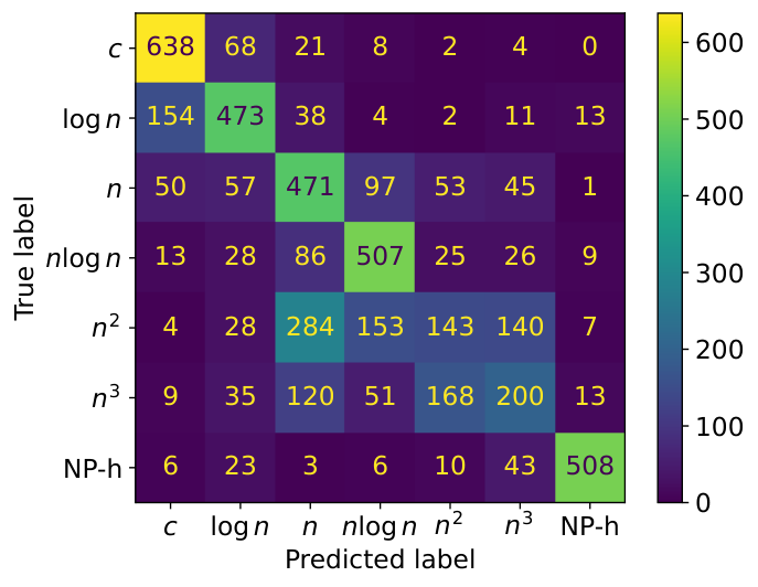
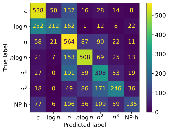
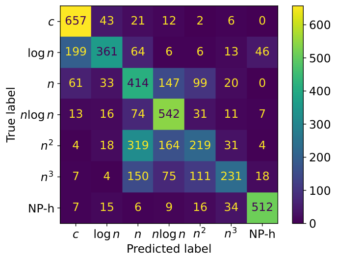
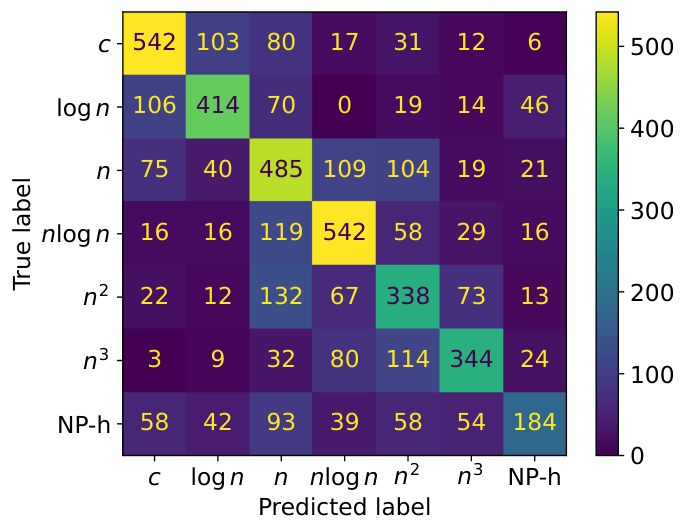
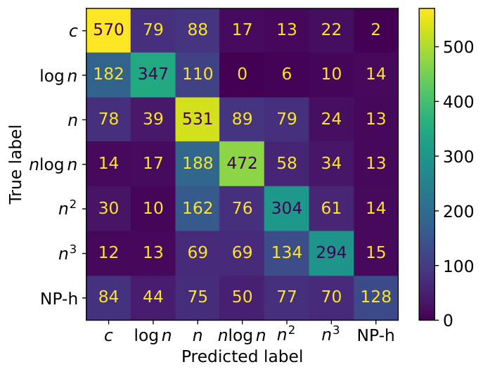
We analyzed the results with responses that could be recognized as one of the seven classes. We can see in Table 6, Table 7 and Table 12, that the constant class and linear class are the most accurate among the classes. The direct correlation between the input size and the number of iterations makes these classes easy to analyze. However, models still face challenges in predicting the complexity of self-referential algorithms and control flows that are not in the main part of the algorithm, such as predicting between the $O(n\log{n})$ class and $O(n^{2})$ class. Failing to analyze loop controls leads to failing to differentiate the $O(n\log n)$ case from $O(n^{2})$. This is well seen in the confusion matrix in Section F, where we can see many wrong predictions are between classes $O(n)$, $O(n\log{n})$, and $O(n^{2})$.

Method	G1	G2	G3	G4	G1	G2	G3	G4
	Java				Python
Decision Tree	57.2	45.6	40.0	38.2	57.2	45.6	40.0	38.2
Random Forest	62.3	46.8	40.6	26.4	62.3	46.8	40.6	26.4
SVM	48.9	18.1	18.1	16.6	48.9	18.1	18.1	16.6
CodeBERT	72.4	62.8	60.7	48.0	56.9	46.9	37.5	22.8
GraphCodeBERT	74.6	61.7	49.8	39.4	60.3	57.8	44.1	30.8
UniXCoder	58.6	54.4	43.2	31.2	58.6	54.4	43.2	31.2
PLBART	74.3	65.1	62.5	52.8	60.6	49.4	39.9	23.2
CodeT5	69.5	56.5	52.4	42.4	53.6	48.1	36.5	19.5
CodeT5+	72.8	63.5	53.0	44.4	56.4	42.4	30.7	29.8

Table 9: Prediction performance on different code length groups.

C.2 Does Problem Description Help?

Model	w/o Desc.		with Desc.
	Ja	Py	Ja	Py
ChatGPT 3.5	43.38	43.14	42.51	36.55
ChatGPT 4.0	55.42	51.57	57.61	54.28

Table 10: Complexity prediction performances of LLMs with and without a problem description in the prompt by the help of information retrieval.

A critical aspect in accurately determining the worst-case time complexity of a given code is the comprehensive understanding of the problem specifications. In certain instances, these specifications may indicate that some inputs are constant, significantly influencing the complexity analysis. The absence of a full and detailed specification can lead to an incomplete or incorrect assessment of the worst-case time complexity. Table 10 shows that problem descriptions actually help LLMs perform better as ChatGPT 4.0 is known to have real-time access to the information on the web. Note that the performance becomes worse for ChatGPT 3.5 when problem IDs are provided, as ChatGPT 3.5 does not utilize the problem descriptions, only from problem IDs.

C.3 Effect of Dead Code Elimination

Model	After		Before
	Ja	Py	Ja	Py
Decision Tree	48.6	38.8	47.6	21.1
Random Forest	43.9	40.8	43.2	23.0
SVM	28.1	23.6	27.1	21.5
CodeBERT	60.5	51.2	59.7	52.0
GraphCodeBERT	60.4	58.1	57.8	60.2
UniXcoder	57.7	55.0	57.2	55.3
PLBART	62.1	54.0	61.2	55.4
CodeT5	60.7	48.9	60.2	49.8
CodeT5+	58.0	49.8	57.4	50.0
ChatGPT 3.5	54.1	45.4	53.8	46.16
ChatGPT 4.0	59.9	53.7	59.7	53.8
Gemini Pro	32.4	35.1	34.0	33.5

Table 11: Performance comparison before and after dead code processing.

Table 11 shows the effect of dead code elimination on prediction performance. Given the nature of codes submitted to competitive programming platforms, there are a lot of redundant variables, methods and even classes in the codes. Due to Java’s complicated IO functions and limited built-in data structures, there are many codes related to the implementation of IO and data structures. Removing such fragments helps the models concentrate on the program structure and results in enhanced prediction accuracy. On the other hand, it appears that the dead code elimination does not help improve the performance on Python as the Python codes are already more concise than the Java codes due to its own language design principle.

Method		Acc	F1	HC	HC2	HC3
Gemini Pro		34.0	31.6	80.2	50.2	63.1
ChatGPT 3.5		49.9	48.6	85.2	63.1	72.8
ChatGPT 4.0		56.9	56.7	88.6	70.1	78.4
Inst	CodeGemma-7B	25.7	28.9	56.7	35.6	44.6
	Gemma2-9B	41.1	43.5	71.5	50.3	58.9
	Gemma2-27B	13.2	17.5	19.8	15.1	17.3
	Gemma1.1-2B	12.8	10.5	53.5	22.6	32.7
	Gemma1.1-7B	25.7	28.7	57.3	34.7	43.8
	Llama3.2-1B	8.2	11.1	24.4	12.0	15.9
	Llama3.2-3B	22.9	22.8	60.6	33.1	43.4
	Llama3.1-8B	30.0	28.4	73.8	43.4	56.6
	Llama3.1-70B	44.2	43.8	81.3	56.2	67.1
	Mistral-12B	42.3	44.3	73.2	53.5	61.9
	Qwen2.5-1.5B	1.4	2.0	4.6	2.2	2.9
	Qwen2.5-7B	34.2	39.9	57.8	42.9	49.3
	Qwen2.5-14B	4.0	7.2	6.6	4.9	5.5
	Qwen2-7B	33.6	31.9	77.1	48.9	61.0
Fine- tuned	CodeGemma-7B	89.5	91.6	94.0	91.4	92.6
	Gemma2-9B	87.4	89.4	93.5	89.3	91.1
	Gemma2-27B	90.2	92.2	94.3	92.0	93.1
	Gemma1.1-2B	84.6	86.5	92.7	88.0	90.0
	Gemma1.1-7B	89.6	91.6	94.0	91.5	92.7
	Llama3.2-1B	83.9	85.2	93.2	87.1	89.8
	Llama3.2-3B	88.2	89.4	94.9	91.1	92.8
	Llama3.1-8B	89.4	90.7	95.4	92.0	93.6
	Llama3.1-70B	92.9	94.1	96.0	94.2	95.0
	Mistral-12B	88.5	89.7	94.8	90.9	92.7
	Qwen2.5-1.5B	88.6	89.8	95.2	91.6	93.3
	Qwen2.5-7B	88.7	90.0	95.0	91.4	93.1
	Qwen2.5-14B	91.9	93.2	96.0	93.6	94.7
	Qwen2-7B	90.2	91.5	95.3	92.5	93.7

Table 12: Complexity prediction with accuracy, macro f1 score, and HC-Score for each LLM models

Appendix D Failure Cases

⬇

public static void main(String[] args) {

Scanner sc = new Scanner(System.in);

int cura = 0, curb = 0;

int ver;

System.out.println("? 0 0");

System.out.flush();

ver = sc.nextInt();

for (int i = 29; i >= 0; i--) {

System.out.println("? " + (cura + (1 << i)) + " " + curb);

System.out.flush();

int temp1 = sc.nextInt();

System.out.println("? " + cura + " " + (curb + (1 << i)));

System.out.flush();

int temp2 = sc.nextInt();

if (temp1 != temp2) {

if (temp2 == 1) {

cura += (1 << i);

curb += (1 << i);

}

} else {

if (ver == 1) cura += (1 << i);

if (ver == -1) curb += (1 << i);

ver = temp1;

}

}

System.out.println("! " + cura + " " + curb);

}

}

The following example exhibits a failure example where our model predicts $O(2^{n})$ for a code with $O(\ln n)$ complexity. We suspect that the primary reason is the usage of bitwise operators. When we filter the codes that use any bitwise operator at least once from our CodeComplex dataset, about 56 of the codes belong to the class $O(2^{n})$. We find that many implementations for exponential problems rely on bitwise operators as they can efficiently manage the backtracking process by manipulating bit-level flags.

The following example demonstrates the case when our model predicts constant time complexity $O(1)$ for a code that runs in $O(n)$ time. We suspect that our model may have ignored the existence of the check method which actually determines the $O(n)$ time complexity or considered the argument of check as constant.

⬇

public static int check(StringBuilder s) {

int countRemove = 0;

if (!s.toString().contains("xxx")) return countRemove;

else {

for (int i = 1; i < s.length() - 1; i++) {

if (s.charAt(i - 1) == ’x’ && s.charAt(i) == ’x’ && s.charAt(i + 1) == ’x’) {

countRemove++;

}

}

return countRemove;

}

}

public static void main(String[] args) {

Scanner sc = new Scanner(System.in);

int n = sc.nextInt();

String s = sc.next();

StringBuilder sb = new StringBuilder("");

sb.append(s);

System.out.println(check(sb));

}

}

The following is the case where our model predicts the quadratic time complexity $O(n^{2})$ when the ground-truth label is $O(n\ln n)$. We guess that our model simply translates the nested for loops into the quadratic time complexity. However, the outer loop is to repeat each test case and therefore should be ignored. Then, the $O(n\ln n)$ complexity can be determined by the sort function used right before the nested loops.

⬇

public static void main(String[] args) {

Scanner sc = new Scanner(System.in);

int n = sc.nextInt();

int[] coins = new int[n];

for (int i = 0; i < n; ++i) coins[i] = sc.nextInt();

Arrays.sort(coins);

int ans = (int) 1e9;

for (int i = 1; i <= n; ++i) {

int sum1 = 0;

int c = 0;

int j = n - 1;

for (j = n - 1; j >= 0 && c < i; --j, ++c) {

sum1 += coins[j];

}

int sum2 = 0;

for (int k = 0; k <= j; ++k) sum2 += coins[k];

if (sum1 > sum2) {

System.out.println(i);

return;

}

}

}

}

The following is the case when our model is confused with exponential complexity $O(2^{n})$ with quadratic complexity $O(n^{2})$. The code actually runs in exponential time in the worst-case but our model simply returns quadratic time complexity as it does not take into account the recursive nature of the method solve.

⬇

static int n, KA, A;

static int[] b;

static int[] l;

static double ans = 0;

public static void main(String[] args) throws IOException {

Scanner in = new Scanner(System.in);

n = in.nextInt();

KA = in.nextInt();

A = in.nextInt();

b = new int[n];

l = new int[n];

for (int i = 0; i < l.length; i++) {

b[i] = in.nextInt();

l[i] = in.nextInt();

}

dp = new double[n + 2][n + 2][n * 9999 + 2];

go(0, KA);

System.out.printf("%.6f\n", ans);

}

public static void go(int at, int k) {

if (at == n) {

ans = Math.max(ans, solve(0, 0, 0));

return;

}

for (int i = 0; i <= k; i++) {

if (l[at] + i * 10 <= 100) {

l[at] += i * 10;

go(at + 1, k - i);

l[at] -= i * 10;

}

}

}

static double dp[][][];

public static double solve(int at, int ok, int B) {

if (at == n) {

if (ok > n / 2) {

return 1;

} else {

return (A * 1.0) / (A * 1.0 + B);

}

}

double ret = ((l[at]) / 100.0) * solve(at + 1, ok + 1, B) + (1.0 - ((l[at]) / 100.0)) * solve(at + 1, ok, B + b[at]);

return ret;

}

}

The following is the case when our model predicts $O(\ln n)$ for a code with $O(n^{2})$ complexity. It is easily seen that the inversions function determines the quadratic time complexity by the nested for loops. We suspect that somehow our model does not take into account the inversions function in the complexity prediction and instead focuses on the modulo () operator to draw the wrong conclusion that the complexity is in $O(\ln n)$.

⬇

public static long inversions(long[] arr) {

long x = 0;

int n = arr.length;

for (int i = n - 2; i >= 0; i--) {

for (int j = i + 1; j < n; j++) {

if (arr[i] > arr[j]) {

x++;

}

}

}

return x;

}

public static void main(String[] args) {

Scanner sc = new Scanner(System.in);

int n = sc.nextInt();

long[] arr = new long[n];

for (int i = 0; i < n; i++) arr[i] = sc.nextLong();

long m = sc.nextLong();

long x = inversions(arr) % 2;

for (int i = 0; i < m; i++) {

int l = sc.nextInt() - 1;

int r = sc.nextInt() - 1;

if ((r - l + 1) % 4 > 1) x = (x + 1) % 2;

if (x == 1) System.out.println("odd");

else System.out.println("even");

}

}

}

Appendix E Further Details on Dead Code Elimination

In a broad sense, the dead code includes redundant code, unreachable code, oxbow code, and so on. We only focus on eliminating unreachable codes, mainly methods and classes that are declared but used nowhere in the code. In order to find such dead codes, we first parse a Java code into an AST and discover methods and classes that do not exist in any method call, class declaration, and arguments of methods. Once we discover such unused methods and classes, we remove the codes corresponding to the declarations of these methods and classes.

The following codes are a running example of the dead code elimination process. From the first code, we can obtain the second code by applying the dead code elimination. It is readily seen that the number of lines decreases from 211 to 101 by the elimination process. In fact, our model predicts $O(\ln n)$ and $O(1)$ for the complexity of the code before and after dead code elimination, respectively, while the actual complexity of the code is $O(1)$.

⬇

static long mod = ((long) 1e9) + 7;

public static int gcd(int a, int b) {

if (b == 0) return a;

else return gcd(b, a % b);

}

public static long pow_mod(long x, long y) {

long res = 1;

x = x % mod;

while (y > 0) {

if ((y & 1) == 1) res = (res * x) % mod;

y = y >> 1;

x = (x * x) % mod;

}

return res;

}

public static int lower_bound(int[] arr, int val) {

int lo = 0;

int hi = arr.length - 1;

while (lo < hi) {

int mid = lo + ((hi - lo + 1) / 2);

if (arr[mid] == val) {

return mid;

} else if (arr[mid] > val) {

hi = mid - 1;

} else lo = mid;

}

if (arr[lo] <= val) return lo;

else return -1;

}

public static int upper_bound(int[] arr, int val) {

int lo = 0;

int hi = arr.length - 1;

while (lo < hi) {

int mid = lo + ((hi - lo) / 2);

if (arr[mid] == val) {

return mid;

} else if (arr[mid] > val) {

hi = mid;

;

} else lo = mid + 1;

}

if (arr[lo] >= val) return lo;

else return -1;

}

public static void main(String[] args) throws java.lang.Exception {

Reader sn = new Reader();

Print p = new Print();

int n = sn.nextInt();

while ((n--) > 0) {

int a = sn.nextInt();

int b = sn.nextInt();

int small = Math.min(a, b);

int large = Math.max(a, b);

long steps = 0;

while (small != 0) {

steps += (long) (large / small);

int large1 = small;

small = large % small;

large = large1;

}

p.printLine(Long.toString(steps));

}

p.close();

}

}

class Pair implements Comparable<Pair> {

int val;

int in;

Pair(int a, int b) {

val = a;

in = b;

}

@Override

public int compareTo(Pair o) {

if (val == o.val) return Integer.compare(in, o.in);

else return Integer.compare(val, o.val);

}

}

class Reader {

final private int BUFFER_SIZE = 1 << 16;

private DataInputStream din;

private byte[] buffer;

private int bufferPointer, bytesRead;

public boolean isSpaceChar(int c) {

return c == ’ ’ || c == ’\n’ || c == ’\r’ || c == ’\t’ || c == -1;

}

public Reader() {

din = new DataInputStream(System.in);

buffer = new byte[BUFFER_SIZE];

bufferPointer = bytesRead = 0;

}

public Reader(String file_name) throws IOException {

din = new DataInputStream(new FileInputStream(file_name));

buffer = new byte[BUFFER_SIZE];

bufferPointer = bytesRead = 0;

}

public String readLine() throws IOException {

byte[] buf = new byte[64];

int cnt = 0, c;

while ((c = read()) != -1) {

if (c == ’\n’) break;

buf[cnt++] = (byte) c;

}

return new String(buf, 0, cnt);

}

public String readWord() throws IOException {

int c = read();

while (isSpaceChar(c)) c = read();

StringBuilder res = new StringBuilder();

do {

res.appendCodePoint(c);

c = read();

} while (!isSpaceChar(c));

return res.toString();

}

public int nextInt() throws IOException {

int ret = 0;

byte c = read();

while (c <= ’ ’) c = read();

boolean neg = (c == ’-’);

if (neg) c = read();

do {

ret = ret * 10 + c - ’0’;

} while ((c = read()) >= ’0’ && c <= ’9’);

if (neg) return -ret;

return ret;

}

public long nextLong() throws IOException {

long ret = 0;

byte c = read();

while (c <= ’ ’) c = read();

boolean neg = (c == ’-’);

if (neg) c = read();

do {

ret = ret * 10 + c - ’0’;

} while ((c = read()) >= ’0’ && c <= ’9’);

if (neg) return -ret;

return ret;

}

public double nextDouble() throws IOException {

double ret = 0, div = 1;

byte c = read();

while (c <= ’ ’) c = read();

boolean neg = (c == ’-’);

if (neg) c = read();

do {

ret = ret * 10 + c - ’0’;

} while ((c = read()) >= ’0’ && c <= ’9’);

if (c == ’.’) {

while ((c = read()) >= ’0’ && c <= ’9’) {

ret += (c - ’0’) / (div *= 10);

}

}

if (neg) return -ret;

return ret;

}

private void fillBuffer() throws IOException {

bytesRead = din.read(buffer, bufferPointer = 0, BUFFER_SIZE);

if (bytesRead == -1) buffer[0] = -1;

}

private byte read() throws IOException {

if (bufferPointer == bytesRead) fillBuffer();

return buffer[bufferPointer++];

}

public void close() throws IOException {

if (din == null) return;

din.close();

}

}

class Print {

private final BufferedWriter bw;

public Print() {

bw = new BufferedWriter(new OutputStreamWriter(System.out));

}

public void print(String str) throws IOException {

bw.append(str);

}

public void printLine(String str) throws IOException {

print(str);

bw.append("\n");

}

public void close() throws IOException {

bw.close();

}

}

Code after Dead Code Elimination:

⬇

public static int gcd(int a, int b) {

if ((b == 0)) return a;

else return gcd(b, (a % b));

}

public static void main(String[] args) throws java.lang.Exception {

Reader sn = new Reader();

Print p = new Print();

int n = sn.nextInt();

while ((n > 0)) {

int a = sn.nextInt();

int b = sn.nextInt();

int small = Math.min(a, b);

int large = Math.max(a, b);

long steps = 0;

while ((small != 0)) {

steps += (long) (large / small);

int large1 = small;

small = (large % small);

large = large1;

}

p.printLine(Long.toString(steps));

}

p.close();

}

class Reader {

final private int BUFFER_SIZE = (1 << 16);

private DataInputStream din;

private byte[] buffer;

private int bufferPointer, bytesRead;

public boolean isSpaceChar(int c) {

return (((((c == ’ ’) || (c == ’\n’)) || (c == ’\r’)) || (c == ’\t’)) || (c == -1));

}

public Reader() {

din = new DataInputStream(System.in);

buffer = new byte[BUFFER_SIZE];

bufferPointer = bytesRead = 0;

}

public Reader(String file_name) throws IOException {

din = new DataInputStream(new FileInputStream(file_name));

buffer = new byte[BUFFER_SIZE];

bufferPointer = bytesRead = 0;

}

public int nextInt() throws IOException {

int ret = 0;

byte c = read();

while ((c <= ’ ’)) c = read();

boolean neg = (c == ’-’);

if (neg) c = read();

do {

ret = (((ret * 10) + c) - ’0’);

} while ((((c = read()) >= ’0’) && (c <= ’9’)));

if (neg) return -ret;

return ret;

}

private void fillBuffer() throws IOException {

bytesRead = din.read(buffer, bufferPointer = 0, BUFFER_SIZE);

if ((bytesRead == -1)) buffer[0] = -1;

}

private byte read() throws IOException {

if ((bufferPointer == bytesRead)) fillBuffer();

return buffer[bufferPointer++];

}

public void close() throws IOException {

if ((din == null)) return;

din.close();

}

}

class Print {

final private BufferedWriter bw;

public Print() {

bw = new BufferedWriter(new OutputStreamWriter(System.out));

}

public void print(String str) throws IOException {

bw.append(str);

}

public void printLine(String str) throws IOException {

print(str);

bw.append("\n");

}

public void close() throws IOException {

bw.close();

}

}

Appendix F Confusion Matrices for Models

Figure 6: Confusion matrices of prediction results by CodeBERT on Java (left) and Python (right) datasets.

Figure 7: Confusion matrices of prediction results by GraphCodeBERT on Java (left) and Python (right) datasets.

Figure 8: Confusion matrices of prediction results by PLBART on Java (left) and Python (right) datasets.

Figure 9: Confusion matrices of prediction results by UniXcoder on Java (left) and Python (right) datasets.

Figure 10: Confusion matrices of prediction results by CodeT5 on Java (left) and Python (right) datasets.

Figure 11: Confusion matrices of prediction results by CodeT5+ on Java (left) and Python (right) datasets.

References

- Ahmad et al. (2021) Wasi Ahmad, Saikat Chakraborty, Baishakhi Ray, and Kai-Wei Chang. 2021. Unified pre-training for program understanding and generation. In Proceedings of the 2021 Conference of the North American Chapter of the Association for Computational Linguistics: Human Language Technologies, pages 2655–2668, Online. Association for Computational Linguistics.
- Austin et al. (2021) Jacob Austin, Augustus Odena, Maxwell I. Nye, Maarten Bosma, Henryk Michalewski, David Dohan, Ellen Jiang, Carrie J. Cai, Michael Terry, Quoc V. Le, and Charles Sutton. 2021. Program synthesis with large language models. CoRR, abs/2108.07732.
- Bentley et al. (1980) Jon Louis Bentley, Dorothea Haken, and James B. Saxe. 1980. A general method for solving divide-and-conquer recurrences. SIGACT News, 12(3):36–44.
- Brown et al. (2020) Tom B. Brown, Benjamin Mann, Nick Ryder, Melanie Subbiah, Jared Kaplan, Prafulla Dhariwal, Arvind Neelakantan, Pranav Shyam, Girish Sastry, Amanda Askell, Sandhini Agarwal, Ariel Herbert-Voss, Gretchen Krueger, Tom Henighan, Rewon Child, Aditya Ramesh, Daniel M. Ziegler, Jeffrey Wu, Clemens Winter, Christopher Hesse, Mark Chen, Eric Sigler, Mateusz Litwin, Scott Gray, Benjamin Chess, Jack Clark, Christopher Berner, Sam McCandlish, Alec Radford, Ilya Sutskever, and Dario Amodei. 2020. Language models are few-shot learners. In Advances in Neural Information Processing Systems 33: Annual Conference on Neural Information Processing Systems, NeurIPS.
- Chowdhery et al. (2023) Aakanksha Chowdhery, Sharan Narang, Jacob Devlin, Maarten Bosma, Gaurav Mishra, Adam Roberts, Paul Barham, Hyung Won Chung, Charles Sutton, Sebastian Gehrmann, Parker Schuh, Kensen Shi, Sasha Tsvyashchenko, Joshua Maynez, Abhishek Rao, Parker Barnes, Yi Tay, Noam Shazeer, Vinodkumar Prabhakaran, Emily Reif, Nan Du, Ben Hutchinson, Reiner Pope, James Bradbury, Jacob Austin, Michael Isard, Guy Gur-Ari, Pengcheng Yin, Toju Duke, Anselm Levskaya, Sanjay Ghemawat, Sunipa Dev, Henryk Michalewski, Xavier Garcia, Vedant Misra, Kevin Robinson, Liam Fedus, Denny Zhou, Daphne Ippolito, David Luan, Hyeontaek Lim, Barret Zoph, Alexander Spiridonov, Ryan Sepassi, David Dohan, Shivani Agrawal, Mark Omernick, Andrew M. Dai, Thanumalayan Sankaranarayana Pillai, Marie Pellat, Aitor Lewkowycz, Erica Moreira, Rewon Child, Oleksandr Polozov, Katherine Lee, Zongwei Zhou, Xuezhi Wang, Brennan Saeta, Mark Diaz, Orhan Firat, Michele Catasta, Jason Wei, Kathy Meier-Hellstern, Douglas Eck, Jeff Dean, Slav Petrov, and Noah Fiedel. 2023. PaLM: Scaling language modeling with pathways. Journal of Machine Learning Research, 24:240:1–240:113.
- Feng et al. (2020) Zhangyin Feng, Daya Guo, Duyu Tang, Nan Duan, Xiaocheng Feng, Ming Gong, Linjun Shou, Bing Qin, Ting Liu, Daxin Jiang, and Ming Zhou. 2020. Codebert: A pre-trained model for programming and natural languages. In Findings of the Association for Computational Linguistics: EMNLP 2020, volume EMNLP 2020 of Findings of ACL, pages 1536–1547. Association for Computational Linguistics.
- Google (2024) Google. 2024. Gemini. https://gemini.google.com/. Accessed: 2023.02.12.
- Guo et al. (2022) Daya Guo, Shuai Lu, Nan Duan, Yanlin Wang, Ming Zhou, and Jian Yin. 2022. UniXcoder: Unified cross-modal pre-training for code representation. In Proceedings of the 60th Annual Meeting of the Association for Computational Linguistics (Volume 1: Long Papers), pages 7212–7225, Dublin, Ireland. Association for Computational Linguistics.
- Guo et al. (2021) Daya Guo, Shuo Ren, Shuai Lu, Zhangyin Feng, Duyu Tang, Shujie Liu, Long Zhou, Nan Duan, Alexey Svyatkovskiy, Shengyu Fu, Michele Tufano, Shao Kun Deng, Colin B. Clement, Dawn Drain, Neel Sundaresan, Jian Yin, Daxin Jiang, and Ming Zhou. 2021. Graphcodebert: Pre-training code representations with data flow. In 9th International Conference on Learning Representations, ICLR 2021, Virtual Event. OpenReview.net.
- Hutter et al. (2014) Frank Hutter, Lin Xu, Holger H. Hoos, and Kevin Leyton-Brown. 2014. Algorithm runtime prediction: Methods & evaluation. Artificial Intelligence, 206:79–111.
- Jain et al. (2021) Naman Jain, Skanda Vaidyanath, Arun Shankar Iyer, Nagarajan Natarajan, Suresh Parthasarathy, Sriram K. Rajamani, and Rahul Sharma. 2021. Jigsaw: Large language models meet program synthesis. CoRR, abs/2112.02969.
- Jiang et al. (2023) Albert Q. Jiang, Alexandre Sablayrolles, Arthur Mensch, Chris Bamford, Devendra Singh Chaplot, Diego de las Casas, Florian Bressand, Gianna Lengyel, Guillaume Lample, Lucile Saulnier, Lélio Renard Lavaud, Marie-Anne Lachaux, Pierre Stock, Teven Le Scao, Thibaut Lavril, Thomas Wang, Timothée Lacroix, and William El Sayed. 2023. Mistral 7b. Preprint, arXiv:2310.06825.
- Li et al. (2022) Yujia Li, David H. Choi, Junyoung Chung, Nate Kushman, Julian Schrittwieser, Rémi Leblond, Tom Eccles, James Keeling, Felix Gimeno, Agustin Dal Lago, Thomas Hubert, Peter Choy, Cyprien de Masson d’Autume, Igor Babuschkin, Xinyun Chen, Po-Sen Huang, Johannes Welbl, Sven Gowal, Alexey Cherepanov, James Molloy, Daniel J. Mankowitz, Esme Sutherland Robson, Pushmeet Kohli, Nando de Freitas, Koray Kavukcuoglu, and Oriol Vinyals. 2022. Competition-level code generation with alphacode. CoRR, abs/2203.07814.
- Loshchilov and Hutter (2019) Ilya Loshchilov and Frank Hutter. 2019. Decoupled Weight Decay Regularization. In 7th International Conference on Learning Representations, ICLR.
- Lu et al. (2021) Shuai Lu, Daya Guo, Shuo Ren, Junjie Huang, Alexey Svyatkovskiy, Ambrosio Blanco, Colin B. Clement, Dawn Drain, Daxin Jiang, Duyu Tang, Ge Li, Lidong Zhou, Linjun Shou, Long Zhou, Michele Tufano, Ming Gong, Ming Zhou, Nan Duan, Neel Sundaresan, Shao Kun Deng, Shengyu Fu, and Shujie Liu. 2021. CodeXGLUE: A machine learning benchmark dataset for code understanding and generation. In Proceedings of the Neural Information Processing Systems Track on Datasets and Benchmarks 1, NeurIPS Datasets and Benchmarks 2021.
- Moudgalya et al. (2023) Kaushik Moudgalya, Ankit Ramakrishnan, Vamsikrishna Chemudupati, and Xing Han Lu. 2023. TASTY: A transformer based approach to space and time complexity. Preprint, arXiv:2305.05379.
- Narayanan et al. (2017) Annamalai Narayanan, Mahinthan Chandramohan, Rajasekar Venkatesan, Lihui Chen, Yang Liu, and Shantanu Jaiswal. 2017. graph2vec: Learning distributed representations of graphs. CoRR, abs/1707.05005.
- Nogueira (2012) Ana Filipa Nogueira. 2012. Predicting software complexity by means of evolutionary testing. In IEEE/ACM International Conference on Automated Software Engineering, ASE’12, pages 402–405. ACM.
- OpenAI (2024) OpenAI. 2024. ChatGPT. https://openai.com/chatgpt/. Accessed: 2024.02.12.
- Peng et al. (2021) Dinglan Peng, Shuxin Zheng, Yatao Li, Guolin Ke, Di He, and Tie-Yan Liu. 2021. How could neural networks understand programs? In Proceedings of the 38th International Conference on Machine Learning, ICML 2021, volume 139 of Proceedings of Machine Learning Research, pages 8476–8486. PMLR.
- Prenner and Robbes (2021) Julian Aron Aron Prenner and Romain Robbes. 2021. Making the most of small software engineering datasets with modern machine learning. IEEE Transactions on Software Engineering, pages 5050–5067.
- Sikka et al. (2020) Jagriti Sikka, Kushal Satya, Yaman Kumar, Shagun Uppal, Rajiv Ratn Shah, and Roger Zimmermann. 2020. Learning based methods for code runtime complexity prediction. In Advances in Information Retrieval - 42nd European Conference on IR Research, ECIR 2020, Proceedings, Part I, volume 12035 of Lecture Notes in Computer Science, pages 313–325. Springer.
- Team et al. (2024) Gemma Team, Thomas Mesnard, Cassidy Hardin, Robert Dadashi, Surya Bhupatiraju, Shreya Pathak, Laurent Sifre, Morgane Rivière, Mihir Sanjay Kale, Juliette Love, Pouya Tafti, Léonard Hussenot, Pier Giuseppe Sessa, Aakanksha Chowdhery, Adam Roberts, Aditya Barua, Alex Botev, Alex Castro-Ros, Ambrose Slone, Amélie Héliou, Andrea Tacchetti, Anna Bulanova, Antonia Paterson, Beth Tsai, Bobak Shahriari, Charline Le Lan, Christopher A. Choquette-Choo, Clément Crepy, Daniel Cer, Daphne Ippolito, David Reid, Elena Buchatskaya, Eric Ni, Eric Noland, Geng Yan, George Tucker, George-Christian Muraru, Grigory Rozhdestvenskiy, Henryk Michalewski, Ian Tenney, Ivan Grishchenko, Jacob Austin, James Keeling, Jane Labanowski, Jean-Baptiste Lespiau, Jeff Stanway, Jenny Brennan, Jeremy Chen, Johan Ferret, Justin Chiu, Justin Mao-Jones, Katherine Lee, Kathy Yu, Katie Millican, Lars Lowe Sjoesund, Lisa Lee, Lucas Dixon, Machel Reid, Maciej Mikuła, Mateo Wirth, Michael Sharman, Nikolai Chinaev, Nithum Thain, Olivier Bachem, Oscar Chang, Oscar Wahltinez, Paige Bailey, Paul Michel, Petko Yotov, Rahma Chaabouni, Ramona Comanescu, Reena Jana, Rohan Anil, Ross McIlroy, Ruibo Liu, Ryan Mullins, Samuel L Smith, Sebastian Borgeaud, Sertan Girgin, Sholto Douglas, Shree Pandya, Siamak Shakeri, Soham De, Ted Klimenko, Tom Hennigan, Vlad Feinberg, Wojciech Stokowiec, Yu hui Chen, Zafarali Ahmed, Zhitao Gong, Tris Warkentin, Ludovic Peran, Minh Giang, Clément Farabet, Oriol Vinyals, Jeff Dean, Koray Kavukcuoglu, Demis Hassabis, Zoubin Ghahramani, Douglas Eck, Joelle Barral, Fernando Pereira, Eli Collins, Armand Joulin, Noah Fiedel, Evan Senter, Alek Andreev, and Kathleen Kenealy. 2024. Gemma: Open models based on gemini research and technology. Preprint, arXiv:2403.08295.
- Touvron et al. (2023) Hugo Touvron, Thibaut Lavril, Gautier Izacard, Xavier Martinet, Marie-Anne Lachaux, Timothée Lacroix, Baptiste Rozière, Naman Goyal, Eric Hambro, Faisal Azhar, Aurelien Rodriguez, Armand Joulin, Edouard Grave, and Guillaume Lample. 2023. Llama: Open and efficient foundation language models. Preprint, arXiv:2302.13971.
- Turing (1936) Alan M. Turing. 1936. On computable numbers, with an application to the Entscheidungsproblem. Proceedings of the London Mathematical Society, 2(42):230–265.
- Wang et al. (2023) Xuezhi Wang, Jason Wei, Dale Schuurmans, Quoc V. Le, Ed H. Chi, Sharan Narang, Aakanksha Chowdhery, and Denny Zhou. 2023. Self-consistency improves chain of thought reasoning in language models. In The Eleventh International Conference on Learning Representations, ICLR.
- Wang et al. (2021) Yue Wang, Weishi Wang, Shafiq Joty, and Steven C.H. Hoi. 2021. CodeT5: Identifier-aware unified pre-trained encoder-decoder models for code understanding and generation. In Proceedings of the 2021 Conference on Empirical Methods in Natural Language Processing, pages 8696–8708, Online and Punta Cana, Dominican Republic. Association for Computational Linguistics.
- Wei et al. (2022) Jason Wei, Xuezhi Wang, Dale Schuurmans, Maarten Bosma, Brian Ichter, Fei Xia, Ed H. Chi, Quoc V. Le, and Denny Zhou. 2022. Chain-of-thought prompting elicits reasoning in large language models. In Advances in Neural Information Processing Systems 35: Annual Conference on Neural Information Processing Systems, NeurIPS.
- Yang et al. (2024) An Yang, Baosong Yang, Binyuan Hui, Bo Zheng, Bowen Yu, Chang Zhou, Chengpeng Li, Chengyuan Li, Dayiheng Liu, Fei Huang, Guanting Dong, Haoran Wei, Huan Lin, Jialong Tang, Jialin Wang, Jian Yang, Jianhong Tu, Jianwei Zhang, Jianxin Ma, Jianxin Yang, Jin Xu, Jingren Zhou, Jinze Bai, Jinzheng He, Junyang Lin, Kai Dang, Keming Lu, Keqin Chen, Kexin Yang, Mei Li, Mingfeng Xue, Na Ni, Pei Zhang, Peng Wang, Ru Peng, Rui Men, Ruize Gao, Runji Lin, Shijie Wang, Shuai Bai, Sinan Tan, Tianhang Zhu, Tianhao Li, Tianyu Liu, Wenbin Ge, Xiaodong Deng, Xiaohuan Zhou, Xingzhang Ren, Xinyu Zhang, Xipin Wei, Xuancheng Ren, Xuejing Liu, Yang Fan, Yang Yao, Yichang Zhang, Yu Wan, Yunfei Chu, Yuqiong Liu, Zeyu Cui, Zhenru Zhang, Zhifang Guo, and Zhihao Fan. 2024. Qwen2 technical report. Preprint, arXiv:2407.10671.
- Yao et al. (2023) Shunyu Yao, Dian Yu, Jeffrey Zhao, Izhak Shafran, Tom Griffiths, Yuan Cao, and Karthik Narasimhan. 2023. Tree of thoughts: Deliberate problem solving with large language models. In Advances in Neural Information Processing Systems, volume 36, pages 11809–11822. Curran Associates, Inc.