An FPGA-Based Accelerator for Graph Embedding using Sequential Training Algorithm

Abstract

A graph embedding is an emerging approach that can represent a graph structure with a fixed-length low-dimensional vector. node2vec is a well-known algorithm to obtain such a graph embedding by sampling neighboring nodes on a given graph with a random walk technique. However, the original node2vec algorithm typically relies on a batch training of graph structures; thus, it is not suited for applications in which the graph structure changes after the deployment. In this paper, we focus on node2vec applications for IoT (Internet of Things) environments. To handle the changes of graph structures after the IoT devices have been deployed in edge environments, in this paper we propose to combine an online sequential training algorithm with node2vec. The proposed sequentially-trainable model is implemented on a resource-limited FPGA (Field-Programmable Gate Array) device to demonstrate the benefits of our approach. The proposed FPGA implementation achieves up to 205.25 times speedup compared to the original model on CPU. Evaluation results using dynamic graphs show that although the original model decreases the accuracy, the proposed sequential model can obtain better graph embedding that can increase the accuracy even when the graph structure is changed.

Keywords node2vec  $\cdot$ OS-ELM  $\cdot$ FPGA

1 Introduction

Graph structures in which nodes are connected by edges can be seen everywhere in our life. For example, friendships of users in social networking services, relationships between users and purchased items in e-commerce sites, paper citation relationships, and chemical representations of atoms and bonds can be represented by such graph structures. Thus, there are high demands for applications that can extract, analyze, and utilize information from these graph structures. Although a graph structure can be represented by an adjacent matrix, the adjacent matrix cannot be directly used in statistical or machine learning based methods especially when the graph structure becomes large and sparse. To overcome this issue, a graph embedding is an emerging representation which can be directly used with statistical or machine learning based methods.

Using the graph embedding, graph structures can be represented with fixed-length low-dimensional vectors. node2vec [1] is a well-known algorithm to obtain the graph embedding by sampling neighboring node information on a given graph with a random walk technique. However, the original node2vec algorithm typically relies on a batch training, not online sequential training; thus, it is not suited for applications where the graph structure changes after the deployment. In this paper, we assume node2vec applications for IoT environments. To handle the changes of graph structures after the IoT devices are deployed in edge environments, in this paper we propose to combine an online sequential training algorithm with node2vec. Since the low-cost and low-power execution is required for such IoT applications, the proposed sequential model is implemented on a resource-limited FPGA device in order to significantly shorten the training time at the deployed environment.

The rest of this paper is organized as follows. Section 2 introduces related works, and Section 3 proposes a sequentially-trainable graph embedding model and its FPGA based accelerator. Section 4 evaluates the model and the accelerator in terms of the execution time, accuracy, model size, and FPGA resource utilization. Section 5 summarizes our contributions.

2 Related Work

2.1 node2vec Algorithm

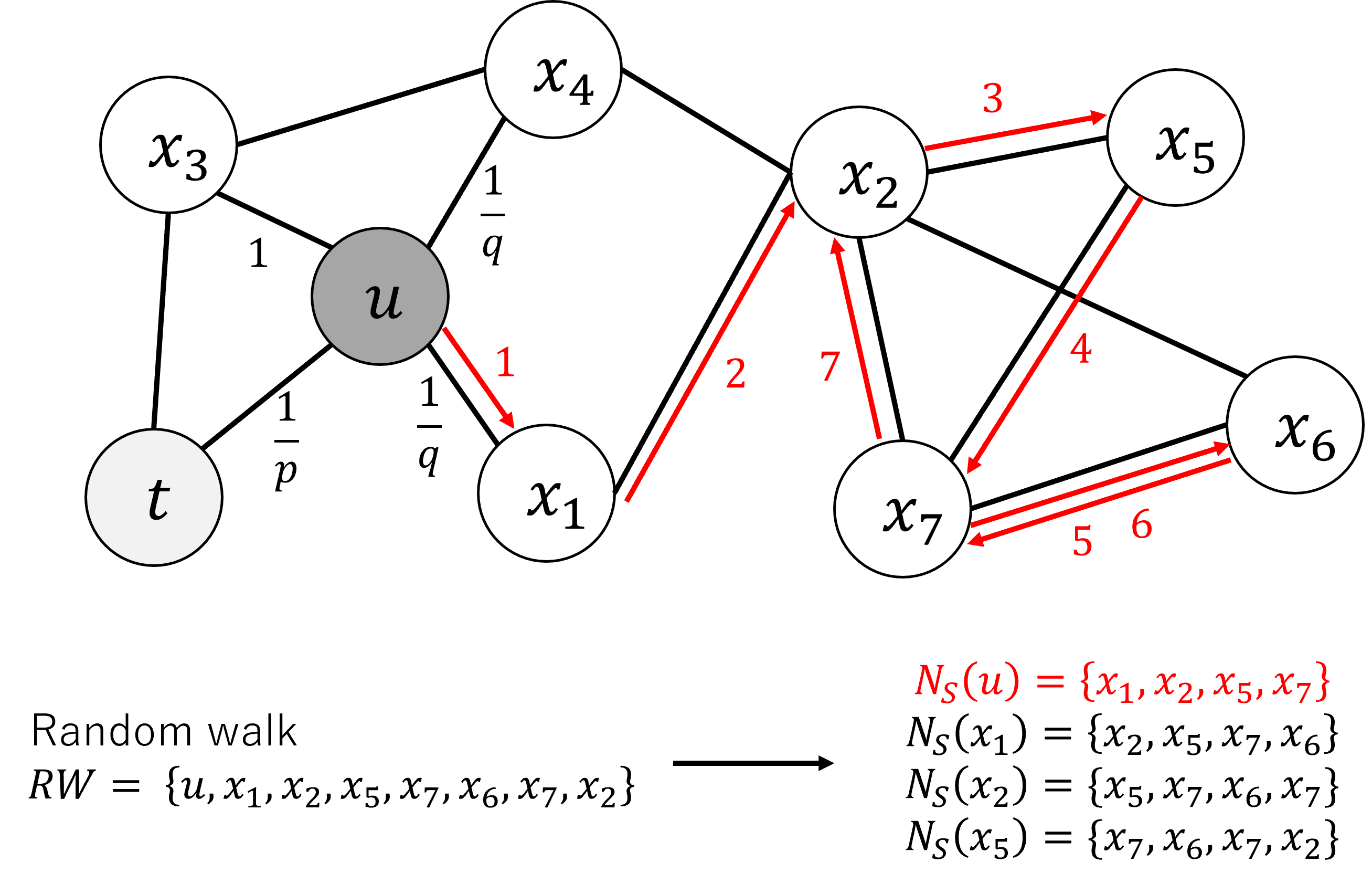
node2vec [1] is a well-known algorithm to obtain a graph embedding. As shown in Figure 1, a random walk is performed from a selected start node (e.g., node-$t$) in the graph in order to collect neighboring nodes information. Assuming that a transition has been performed from node-$t$ to node-$u$, Figure 1 illustrates the next transition probabilities from node-$u$ to one of its adjacent nodes. The transition probabilities to the adjacent nodes are determined as follows.

Figure 1: An example of random walk in node2vec

$$P(c_{i}=x|c_{i-1}=u)=\left\{\begin{aligned} \frac{\alpha_{pq}(t,x)w_{ux}}{Z}\quad\text{if}\quad((u,x)\in E)\\ 0,\qquad\quad\quad\text{if}\quad((u,x)\notin E)\end{aligned}\right.$$ (1)

where $c_{i}$ represents the $i$-th node during a random walk. $(u,x)$ represents an edge between node-$u$ and node-$x$, and $w_{ux}$ represents the weight of this edge. $E$ represents all the edges in a graph. $Z$ is a normalizing constant. $\alpha$ is defined using parameters $p$ and $q$ as follows.

$$\alpha_{pq}(t,x)=\left\{\begin{aligned} 1\>/\>p\quad\text{if}\quad d_{tx}=0\\ 1\quad\quad\text{if}\quad d_{tx}=1\\ 1\>/\>q,\quad\text{if}\quad d_{tx}=2\\ \end{aligned}\right.$$ (2)

where $d_{tx}$ represents a distance between the previous node (i.e., node-$t$) and the next node (i.e., node-$x$). That is, $d_{tx}$ is set to 0 when transitioning back to node-$t$; $d_{tx}$ is set to 1 when transitioning to an adjacent node of node-$t$; otherwise $d_{tx}$ is set to 2. Let $RW$ be the result of a single random walk. The training samples can be efficiently generated by partitioning $RW$ with a given context size (i.e., window size). In Figure 1, $N_{S}(u)$ is an example of the training samples. $N_{S}(u)$ represents neighboring nodes of node-$u$ obtained by a random walk started from node-$u$ based on a random walk strategy $S$. These training samples are trained with the skip-gram model [2] illustrated in Figure 2 (left).

In the skip-gram model, the numbers of input- and output-layer nodes are the same as the number of nodes in the graph. The number of hidden-layer nodes is corresponding to the number of the graph embedding dimensions to be trained. An input data to the skip-gram model is a one-hot vector, where only node-$u$ is 1 and the other nodes are 0. An output of the model is a vector, where each node represents a probability that this node appears as an adjacent of node of node-$u$. From $N_{S}(u)$ we can obtain four different teacher labels, each of which is a one-hot vector, where one of nodes $x_{1}$, $x_{2}$, $x_{5}$, and $x_{7}$ is 1 and the other nodes are 0. Since there are four different teacher labels, the final loss value is calculated by summing up the four loss values computed using the same weights but different one-hot teacher labels.

node2vec is widely used for the graph embedding for various applications including those for IoT environments. For example, node2vec is used to detect malware in IoT environments [3]; it can also be used to predict the usage pattern in IoT environments [4].

2.2 Sequential Training Algorithm

OS-ELM (Online Sequential Extreme Learning Machine) [5] is an online sequential training algorithm for neural networks with a single hidden layer. Figure 3 illustrates the network structure and its training algorithm. In the OS-ELM algorithm, the input-side weights $\alpha$ are fixed at random values at the initialization time, and only the output-side weights $\beta$ are trainable and sequentially updated. Assuming that the $i$-th input data is fed to the neural network, the hidden-layer outputs $H_{i}$ are generated. Then, the output-side weights $\beta_{i}$ are calculated based on previous weights $\beta_{i-1}$ and temporary values $P_{i}$, which are also calculated based on previous values $P_{i-1}$ and $H_{i}$. As shown in the equations in the figure, the OS-ELM algorithm derives an optimal $\beta$ that can minimize a loss between final outputs $G(x_{i}\alpha+b)\beta$ and teacher labels $y_{i}$ analytically. The sequential training is simple and fast since the sequential training is done in a single epoch, which is different from conventional backpropagation based training.

Figure 2: Original skip-gram model (left) and proposed model (right)

Figure 3: OS-ELM algorithm

2.3 node2vec Accelerator

Several FPGA implementations of node2vec have been reported. For example, an FPGA based acceleration of random walk of node2vec is reported [6]. An FPGA based acceleration of word2vec [2] that uses the skip-gram model as well as node2vec is also reported [7]. Please note that the random walk is accelerated in [6] while in this paper we accelerate the training algorithm of node2vec. Although the training algorithm of word2vec is accelerated by FPGA in [7], in this paper we newly propose a sequential training of node2vec for dynamic graphs by combining OS-ELM and the skip-gram so that the on-device training can be efficiently implemented on resource-limited FPGA devices.

3 Sequential Graph Embedding Accelerator

In this section, we propose a sequentially-trainable skip-gram model using OS-ELM for node2vec applications. Then, we illustrate the FPGA implementation of the proposed model.

3.1 Sequentially-Trainable Skip-Gram Model

Figure 2 (right) illustrates the proposed OS-ELM based training model for graph embedding, and Algorithm 1 describes the training algorithm. Since both the skip-gram and OS-ELM assume neural networks with a single hidden layer, the OS-ELM algorithm can be theoretically applied to the skip-gram. In the original OS-ELM, $H_{i}$ in Algorithm 1 are calculated using $x_{i}$; specifically, $H_{i}=G(x_{i}\alpha+b)$. Since the input vector $x_{i}$ is one-hot, $H_{i}$ can be calculated as the row vector corresponding to the center node which is extracted from $\alpha$ assuming that $b$ is zero.

In the skip-gram model, the desired graph embedding is obtained from the weights of the network. Specifically, we may be able to use the following weights for the graph embedding: 1) the input-side weights $\alpha$, 2) the output-side weights $\beta$, and 3) the average of $\alpha$ and $\beta$. Among them, the input-side weights are typically used for graph embedding. However, since the input-side weights of the original OS-ELM are statically fixed at random values, in the proposed model we cannot directly use the input-side weights for the graph embedding. Although the original skip-gram model uses the input-side weights for the graph embedding, in the proposed model we utilize the trainable weights of OS-ELM (i.e., $\beta$) to build the input-side weights as in [8]. Please note that although this method is not suited for word2vec [8], it can be applied for node2vec algorithm. In Figure 2, $\mu$ is a scale factor to transform $\beta$ into the input-side weights. In this case, the input-side weights become a constant multiple of $\beta$; thus, the hidden-layer outputs $H_{i}$ also become a constant multiple of the column vector corresponding to the center node which is extracted from $\beta$. This eliminates the original random weights $\alpha$ from OS-ELM, so we can reduce the model size and memory utilization.

The proposed model adopts the negative sampling [9]. In this case, only a fraction of samples from negative nodes of teacher labels (i.e., nodes with a value of 0 in the one-hot vector) is trained without training all the negative samples. This can significantly reduce the training time by limiting the number of nodes to update, even if the number of nodes in the graph is huge. In general, 5 to 20 negative samples are sufficient for small datasets, while 2 to 5 negative samples are enough for large datasets [9]. In Algorithm 1, the innermost loop starting from line 9 shows the negative sampling. The outermost loop starting from line 1 processes $RW$ obtained from a random walk of node2vec. In the training phase, as described in Section 2.1, $RW$ is partitioned into samples (e.g., $N_{S}(u)$) by a given window size. In the case of $N_{S}(u)$, for example, node-$u$ is the center node, and nodes included in $N_{S}(u)$ are trained as positive nodes. Only a fraction of negative nodes is sampled randomly by the negative sampling method. The sampled frequency as negative nodes depends on the number of appearances of each node in the entire $RW$. This sampling is done by the Walker’s alias, which is a weighted sampling method. In this case, although the time complexity to build a table used in the sampling is proportional to the number of nodes, the sampling can be done in $O(1)$ time complexity. In Algorithm 1, lines 2 to 7 and lines 14 to 15 describe the training algorithm of OS-ELM.

Algorithm 1 Proposed algorithm

1:for each context do

2:     $H_{i}\leftarrow\beta[$ center node $]\times\mu$

3:     Compute $P_{i-1}H_{i}^{T}$ and $H_{i}P_{i-1}$

4:     Compute $P_{i-1}H_{i}^{T}H_{i}P_{i-1}$ and $H_{i}P_{i-1}H_{i}^{T}$

5:     $hpht\_inv\leftarrow\frac{1}{H_{i}P_{i-1}H_{i}^{T}}$

6:     $P_{i}\leftarrow P_{i-1}-P_{i-1}H_{i}^{T}H_{i}P_{i-1}\times hpht\_inv$

7:     Compute $P_{i}H_{i}^{T}$

8:     for each window do

9:         for $itr=1$ to $ns+1$ do

10:              if $itr=1$ :

11:                  $sample\leftarrow$ positive sample

12:              else

13:                  $sample\leftarrow$ negative sample               

14:              Compute $y_{i}-H_{i}\beta_{i-1}[sample]$               

15:     $\beta_{i}\leftarrow\beta_{i-1}+P_{i}H_{i}^{T}(y_{i}-H_{i}\beta_{i-1})$

3.2 FPGA Implementation

In this section, we describe an FPGA implementation of the proposed model. As graphs become larger and the dimensions of graph embedding to be learned increase, it becomes challenging to implement all the weights on resource-limited FPGA devices. In the proposed model, since only a fraction of weights is updated by each training data by the negative sampling, only weights necessary for training are implemented on BRAM cells of the programmable logic part of FPGA. The training process is as follows. First, nodes are sampled from a graph using random walk by the CPU. The obtained result of a single random walk and negative samples necessary for training are pre-sampled by the CPU. These samples are transferred to the programmable logic part via a DMA controller. In the programmable logic part, after receiving the training data and negative samples, weights necessary for training (e.g., $\beta$) are transferred from DRAM to BRAM. Then the model is trained, and weights are updated using these data. Finally, the trained weights are written back to the DRAM. The trained result is also transferred to the DRAM via the DMA controller. By repeating this procedure, a graph embedding can be trained. In our implementation, the same negative samples are used for multiple sets of training data as in [10] to reduce the data transfer between DRAM and BRAM; in this case, training samples obtained by a single random walk are trained using the same negative samples.

To further speedup, a dataflow optimization is applied by modifying the update procedure of $\beta$ in Algorithm 1. Algorithm 2 shows the modified procedure. In Algorithm 1, $P_{i}$ and $\beta_{i}$ are updated sequentially in each iteration (line 1). Since there is a dependency between two successive iterations, a dataflow optimization cannot be applied in our original algorithm. In Algorithm 2, on the other hand, $P$ and $\beta$ are updated outside the outermost loop (lines 19 and 20), and only their accumulated differences (i.e., $\Delta P$ and $\Delta\beta$) are updated sequentially inside the loop. This modification enables the dataflow optimization. Please note that the proposed model is trained with the same output-side weights $\beta$ and the same intermediate data $P$ for the result of a single random walk. It is expected that the proposed model can maintain an accuracy if the number of training data is sufficient, which will be evaluated in the next section.

Algorithm 2 Modified algorithm for dataflow optimization

1:for each context do

2:     $Stage1:$

3:     $\quad\>\>H_{i}\leftarrow\beta[$ center note $]\times\mu$

4:           Compute $P_{i-1}H_{i}^{T}$ and $H_{i}P_{i-1}$

5:     $Stage2:$

6:           Compute $P_{i-1}H_{i}^{T}H_{i}P_{i-1}$ and $H_{i}P_{i-1}H_{i}^{T}$

7:     $Stage3:$      

8:         for each window do

9:              for $itr=1$ to $ns+1$ do

10:                  if $itr=1$ :

11:                       $sample\leftarrow$ positive sample

12:                  else

13:                       $sample\leftarrow$ negative sample                   

14:                  Compute $y_{i}-H_{i}\beta_{i-1}[sample]$                             

15:     $Stage4:$

16:     $\quad\>\>hpht\_inv\leftarrow\frac{1}{H_{i}P_{i-1}H_{i}^{T}}$

17:     $\quad\>\>\Delta P\leftarrow\Delta P-P_{i-1}H_{i}^{T}H_{i}P_{i-1}\times hpht\_inv$

18:     $\quad\>\>\Delta\beta\leftarrow\Delta\beta+P_{i}H_{i}^{T}(y_{i}-H_{i}\beta_{i-1})$

19:$P_{i}\leftarrow P_{i-1}+\Delta P$

20:$\beta_{i}\leftarrow\beta_{i-1}+\Delta\beta$

Table 1: Three datasets used in evaluations

Dataset	# nodes	# edges	# classes
Cora	2708	5429	7
Amazon Photo	7650	143663	8
Amazon Electronics Computers	13752	287209	10

4 Evaluations

In this section, we evaluate the proposed FPGA based accelerator described in Section 3. The proposed accelerator is implemented with Xilinx Vivado v2022.1 and Xilinx Vitis HLS v2022.1. We choose Xilinx Zynq UltraScale+ MPSoC series as a target FPGA platform; specifically, ZCU104 evaluation board (XCZU7EV-2FFVC1156) is used in this paper. As for software counterparts running on CPU, we use C/C++ to implement the models and compile them with gcc 9.4.0. In the performance evaluation, our FPGA implementation is compared with an embedded CPU of the FPGA board (ARM Cortex-A53 @1.2GHz) and a desktop computer (Intel Core i7-11700 @2.5GHz). Ubuntu 20.04.6 LTS in running on the computers.

Table 2: Hyper-parameters of node2vec

p	q	r	l	w	# negative samples
0.5	1.0	10	80	8	10

Table 3: Training time of a single random walk (vs. Cortex-A53 CPU)

	# graph embedding dimensions
	32	64	96
Original model on CPU (ms)	35.357	100.291	202.175
Proposed model on CPU (ms)	18.753	35.941	72.612
Proposed model on FPGA (ms)	0.777	0.878	0.985
Speedup (vs. Original model on CPU)	45.504	114.227	205.254
Speedup (vs. Proposed model on CPU)	24.135	40.935	73.718

4.1 Datasets

Table 1 lists three datasets used in our evaluations. We use Cora [11], Amazon Photo [12], and Amazon Electronics Computers [12]. Cora is a paper citation network in a machine learning research field. Each node represents a paper, and each edge represents a citation relationship. Amazon Photo and Amazon Electronics Computers are subsets of Amazon co-purchase graph dataset [13]. Each node represents a product, and each edge represents that the two products are frequently bought together.

4.2 Execution Time

Here, we evaluate the execution time of the proposed accelerator. The execution time is an elapsed time to train $RW$, which is obtained by a single random walk as mentioned in Section 3. In our evaluation, the length of random walk $l$ and the window size $w$ are set to 80 and 8, respectively. Thus, the training time of a single random walk is measured over 73 iterations of the outermost loop starting from line 1 in Algorithm 2. Table 2 summarizes the other hyper-parameters. The clock frequency of the programmable logic part of the FPGA board is set to 200MHz.

Table 4: Training time of a single random walk (vs. Core i7 CPU)

	# graph embedding dimensions
	32	64	96
Original model on CPU (ms)	1.309	2.293	3.285
Proposed model on CPU (ms)	0.787	1.426	2.396
Proposed model on FPGA (ms)	0.777	0.878	0.985
Speedup (vs. Original model on CPU)	1.687	2.612	3.335
Speedup (vs. Proposed model on CPU)	1.013	1.624	2.432

Table 3 shows the execution times of the proposed accelerator and software implementations on ARM Cortex-A53 CPU. As shown, 1.89 to 2.77 times speedup is achieved by replacing the original skip-gram model with our OS-ELM based sequential model. By implementing the proposed model on the FPGA, the proposed accelerator achieves 24.14 to 73.72 times speedup compared to that on ARM Cortex-A53 CPU. Compared to the CPU implementation of the original skip-gram model, our accelerator achieves 45.50 to 205.25 times speedup. In addition, Table 4 shows the execution times of the proposed accelerator and software implementations on Intel Core i7 11700 CPU. Even when compared to the desktop computer, our small FPGA implementation achieves 1.01 to 3.34 times speedup.

4.3 Accuracy

For the accuracy evaluation, our trained graph embedding is then used for a one-vs-rest logistic regression. The F1 score by the logistic regression is used as an evaluation metric. For the logistic regression, 90% of the data are used as training data, and 10% are used as test data for multiclass classification. SGD (Stochastic Gradient Descent) is used to train the original skip-gram model, and the learning rate is set to 0.01. In this evaluation, a graph embedding is trained three times. An average F1 score over the three trials is reported as the evaluation result.

4.3.1 Impact of Dataflow Optimization

To evaluate the impact of dataflow optimization applied to our FPGA accelerator, the CPU and FPGA implementations of the proposed model are compared in terms of the accuracy. The three datasets described in Section 4.1 are used for this evaluation.

Figure 4 shows the evaluation results, where “ampt” and “amcp” represent Amazon Photo and Amazon Electronics Computers datasets, respectively. While the accuracy of the FPGA implementation decreases by up to 1.09% in Cora dataset, no accuracy degradation is observed in the other two datasets, which have a relatively large number of nodes. In our FPGA implementation, the number of weight updates is decreased due to the dataflow optimization, and this affects the accuracy of Cora, which is a relatively small graph.

(a) CPU vs. FPGA (micro F1 score)

(a) CPU vs. FPGA (micro F1 score)

(b) CPU vs. FPGA (macro F1 score)

Figure 4: Impact of dataflow optimization on accuracy

(a) Cora (micro F1 score)

(b) Amazon Photo (micro F1 score)

(c) Amazon Electronics Computers (micro F1 score)

(d) Cora (macro F1 score)

(e) Amazon Photo (macro F1 score)

(a) Cora (micro F1 score)

(b) Amazon Photo (micro F1 score)

(c) Amazon Electronics Computers (micro F1 score)

(d) Cora (macro F1 score)

(e) Amazon Photo (macro F1 score)

(f) Amazon Electronics Computers (macro F1 score)

Figure 5: Impact of sequential training on accuracy

4.3.2 Impact of Sequential Training

Next, we evaluate the benefit of the sequential training, which is one of the contributions of this paper. Figure 5 shows the evaluation results, where “Original” represents the original skip-gram model and “Proposed” represents the proposed model. In addition, we examine two training scenarios: “all” and “seq”. In the “all” case, an entire graph is trained assuming that all the edges exist from the beginning. In the “seq” case, only a fraction of edges is trained first; then, new edges are sequentially added to the graph, and a sequential training is executed every time a new edge is added. As the initial graph of the “seq” case, we remove edges from an entire graph so that the initial graph becomes a forest without changing the number of connected components to the original entire graph. Subsequently, every time the removed edge is added, the random walk and training of node2vec are executed. In this case, the random walk starts from both the ends of an added edge.

As shown in Figure 5, in the “all” case, the original skip-gram model achieves a higher accuracy compared with the proposed model for all the numbers of graph embedding dimensions (i.e., the numbers of hidden-layer nodes) in all the datasets. In the “seq” case, on the other hand, the accuracy of our OS-ELM based sequentially-trainable model tends to be high compared to the original skip-gram model. In contrast, the accuracy of the original model drops when sequentially training the edges in the “seq” case. This implies that the sequential training using the backpropagation algorithm for the original model causes a catastrophic forgetting. This impact tends to be larger when the number of graph embedding dimensions increases and the graph becomes large. Although in this evaluation only a fraction of weights is updated by the negative sampling, the accuracy of the original model decreases due to the catastrophic forgetting. Please note that the proposed model in the “seq” case achieves a higher accuracy compared to the “all” case. Because in the “seq” case, a random walk and sequential training are executed every time a new edge is added, the number of training samples increases in the “seq” case; thus, the proposed sequential model successfully increases the accuracy. These results demonstrate that the graph embedding can be sequentially trained by using the proposed sequential model even if target graphs are large and dynamically updated.

4.3.3 Impact of Scale Factor $\mu$

As proposed in Section 3.1, in our sequential model, the input-side weights are replaced with a constant multiple of $\beta$. Figure 6 shows the accuracy of the proposed model when the scale factor $\mu$ in Algorithm 2 is varied. Y-axis shows the accuracy, while X-axis shows the scale factor. The number of graph embedding dimensions is 32. In this graph, “alpha” represents an accuracy of a special case, where the input-side weights are fixed with random values as in the original OS-ELM algorithm. The accuracy of this “alpha” case is lower than our proposed model except when the scale factor $\mu$ is very small (i.e., 0.001). Actually, the accuracy of the proposed model when $\mu$ is 0.001 is quite low, indicating that a meaningful graph embedding may not be learned. On the other hand, we can see that the proposed model when $\mu\geq 0.005$ can learn a useful graph embedding. Especially, the accuracy is quite high when $\mu$ is ranging from 0.005 to 0.1, while it is gradually decreased when $\mu>0.1$.

Figure 6: Impact on scale factor $\mu$ on accuracy

Figure 7: Impact of update frequency of sampling table on accuracy

4.3.4 Impact of Update Frequency of Sampling Table

In our proposed model, a table for the negative sampling is updated during the sequential training. Here, we evaluate the impact of the update frequency of the sampling table in terms of the accuracy. For the negative sampling, as mentioned in Section 3.1, the sampling frequency depends on the number of appearances of each node in a given training dataset. Since Walker’s alias is used for the sampling, the time complexity to update the table is proportional to the number of graph nodes. Figure 7 shows the accuracy of the proposed model when the update frequency of the sampling table is varied. Y-axis shows the accuracy, while X-axis shows the number of added edges for each table update (i.e., update frequency of the table). In this graph, “no_change” represents an accuracy of a special case, where the table is not updated once the table is created. The accuracy when the table is updated every 100 edges added is almost the same as that when the table is updated every single edge added. On the other hand, the accuracy is dropped when the table is updated every 10,000 edges added, and that of “no_update” is also low. These negative impacts tend to be large in larger graphs.

Table 5: Model sizes of original model and proposed model (MB)

# graph embedding dimensions	Original model			Proposed model
	cora	ampt	amcp	cora	ampt	amcp
32	1.354	3.823	6.783	0.376	1.088	1.897
64	2.676	7.559	13.589	0.735	2.017	3.600
96	3.999	11.295	20.303	1.105	2.990	5.318

4.4 Model Size

Here, we compare the original skip-gram model and our proposed sequential model for FPGA in terms of the model size. Table 5 shows their model sizes. The results show that the proposed model is up to 3.82 times smaller than the original model, thanks to our simplified OS-ELM based model, where the output-side weights $\beta$ are reused for the input-side weights (thus we do not have to retain $\alpha$). This reduces the memory consumption compared to the original skip-gram model; thus, our proposed model is beneficial for resource-limited IoT devices.

4.5 FPGA Resource Utilization

Here, we evaluate the FPGA resource utilization of the proposed model. We use Zynq UltraScale+ XCZU7EV as a target FPGA device which has 11Mb BRAM and 1,728 DSP slices. Table 6 shows the resource utilizations when the numbers of graph embedding dimensions are 32, 64, and 96.

Table 6: Resource utilizations on XCZU7EV

# graph embedding dimensions	BRAM	DSP	FF	LUT
32	183 (58.65%)	1379 (79.80%)	48609 (10.55%)	53330 (23.15%)
64	271 (86.86%)	1552 (89.81%)	77584 (16.84%)	87901 (38.15%)
96	272 (87.18%)	1573 (91.03%)	86081 (18.68%)	108639 (47.15%)

In our FPGA implementation, the computational parallelism is basically set to 32. However, when the numbers of graph embedding dimensions are 64 and 96, the parallelism is partially set to 48 and 64 so that execution times of pipeline stages are equalized for the dataflow optimization. As shown in the table, when the number of graph embedding dimensions is 32, 79.80% of DSP slices are consumed because fixed-point multiply-add operations are parallelized. When the number of graph embedding dimensions is 64, since the number of BRAM partitions is increased for further speedup, the BRAM and DSP utilizations are 86.86% and 89.81%, respectively. In our implementation, although only the weights which are necessary for the sequential training are implemented on the programmable logic part of the FPGA, the resource utilization is already high. A further speedup by higher parallelism would be possible if more BRAM and DSP resources are available.

5 Summary

In this paper, we proposed an OS-ELM based sequentially-trainable model for graph embedding and implemented it on a resource-limited FPGA device. Compared to the original skip-gram model, the proposed model achieved 1.89 to 2.77 times speedup. Furthermore, the FPGA implementation achieved 45.50 to 205.25 times speedup compared to the original model on CPU. In the proposed model, by replacing the input-side weights with trained output-side weights (i.e., $\beta$), we achieved both the accuracy improvement and the memory size reduction. For the sequential training of dynamic graphs, we showed that although the original model decreases the accuracy, the proposed model can be trained without decreasing the accuracy. Our future plans include comparisons to the original and proposed models on embedded GPU devices to demonstrate the energy efficiency of the proposed FPGA accelerator.

References

- [1] Aditya Grover and Leskovec Jure. Node2vec: Scalable Feature Learning for Networks. In Proceedings of the ACM International Conference on Knowledge Discovery and Data Mining (SIGKDD), pages 855–864, August 2016.
- [2] Tomas Mikolov, Kai Chen, Greg Corrado, and Jeffrey Dean. Efficient Estimation of Word Representations in Vector Space. arXiv Preprint 1301.3781, September 2013.
- [3] Yanchen Qiao, Weizhe Zhang, Xiaojiang Du, and Mohsen Guizani. Malware classification based on multilayer perception and Word2Vec for IoT security. ACM Transactions on Internet Technology (TOIT), 22(1):1–22, 2021.
- [4] Seonghee Kim, Yongyoon Suh, and Hakyeon Lee. What IoT devices and applications should be connected? Predicting user behaviors of IoT services with node2vec embedding. Information Processing and Management, 59(2):102869, 2022.
- [5] Nan-Ying Liang, Guang-Bin Huang, P. Saratchandran, and N. Sundararajan. A Fast and Accurate Online Sequential Learning Algorithm for Feedforward Networks. IEEE Transactions on Neural Networks, 17(6):1411–1423, November 2006.
- [6] Hongshi Tan, Xinyu Chen, Yao Chen, Bingsheng He, and Weng fai Wong. LightRW: FPGA Accelerated Graph Dynamic Random Walks. In Proceedings of the ACM Management of Data, number 1, pages 1–27, 2023.
- [7] Taisuke Ono, Tomoki Shoji, Muthumala Hasitha Waidyasooriya, Masanori Hariyama, Yuichiro Aoki, Yuki Kondoh, and Yaoko Nagasawa. FPGA-Based Acceleration of Word2vec using OpenCL. In Proceedings of the IEEE International Symposium on Circuits and System (ISCAS), pages 1–5, 2019.
- [8] Ofir Press and Lior Wolf. Using the Output Embedding to Improve Language Models. arXiv preprint arXiv:1608.05859, February 2017.
- [9] Tomas Mikolov, Ilya Sutskever, Kai Chen, Greg Corrado, and Jeffrey Dean. Distributed Representations of Words and Phrases and their Compositionality. In Proceedings of the International Conference on Neural Information Processing Systems (NeurIPS), volume 2, pages 3111–3119, December 2013.
- [10] Shihao Ji, Nadathur Satish, Sheng Li, and Pradeep Dubey. Parallelizing word2vec in shared and distributed memory. IEEE Transactions on Parallel and Distributed Systems, 30(9):2090–2100, 2019.
- [11] Andrew Kachites, McCallum Kamal Nigram, Jason Rennie, and Kristie Seymore. Automating the construction of internet portals with machine learning. Information Retrieval, 3:127–163, 2000.
- [12] Oleksandr Shchur, Maximilian Mumme, Aleksandar Bojchevski, and Stephan Günnemman. Pitfalls of graph neural network evaluation. arXiv preprint arXiv:1811.05868, November 2018.
- [13] Julian McAuley, Christopher Targett, Qingfeng Shi, and Anton van den Hengel. Image-based recommendations on styles and substitutes. In Proceedings of the International ACM Conference on Research and Development in Information Retrieval (SIGIR), pages 43–52, 2015.