

Diagnosing and Rectifying Fake OOD Invariance: A Restructured
Causal Approach
Abstract
Invariant representation learning (IRL) encourages the prediction from invariant causal features to labels deconfounded from the environments, advancing the technical roadmap of out-of-distribution (OOD) generalization. Despite spotlights around, recent theoretical result verified that some causal features recovered by IRLs merely pretend domain-invariantly in the training environments but fail in unseen domains. The fake invariance severely endangers OOD generalization since the trustful objective can not be diagnosed and existing causal remedies are invalid to rectify. In this paper, we review a IRL family (InvRat) under the Partially and Fully Informative Invariant Feature Structural Causal Models (PIIF SCM /FIIF SCM) respectively, to certify their weaknesses in representing fake invariant features, then, unify their causal diagrams to propose ReStructured SCM (RS-SCM). RS-SCM can ideally rebuild the spurious and the fake invariant features simultaneously. Given this, we further develop an approach based on conditional mutual information with respect to RS-SCM, then rigorously rectify the spurious and fake invariant effects. It can be easily implemented by a small feature selection subnet introduced in the IRL family, which is alternatively optimized to achieve our goal. Experiments verified the superiority of our approach to fight against the fake invariant issue across a variety of OOD generalization benchmarks.
1Jinan University, 2Sun Yat-sen University, 3Pazhou Lab
c.ziliang@yahoo.com, z.yongsensmile@gmail.com, {laizhr,Gql}@jnu.edu.cn, linliang@ieee.org
Introduction
A fundamental pressumption of machine learning widely believes that models are trained and tested with samples identically and independently (i.i.d.) drawn from a distribution. Whereas in practice, the models are inevitably trained and deployed in ubiquitous scenarios so that they poorly perform than what was expected, due to the violation of the i.i.d. condition inducing distributional shift across various scenarios. The failure could be understood from the view of representation learning, where the i.i.d. condition typically achieves the feature generalizing in a distribution, but unfortunately, at the sacrifice of generalization beyond this observed distribution. It is obviously impossible to obtain the domain universe by collecting data from all scenarios, so how to learn reprsentation with limited observed domains for chasing the invariant performance to unseen domains, have gradually become the promising trend known as invariant representation learning (IRL) for out-of-distribution (OOD) generalization (Shen et al. 2021; Wang et al. 2022a).
The emergence of IRL dates back to approaches for domain adaptation (Ganin et al. 2016; Zhao et al. 2019) where data drawn from a test domain (so-called target domain) can be accessed to quantify the distributional shift, thus, invariant representation is spontaneously obtained while minimizing the domain shift. In the OOD generalization setup, only a few number of domains are available whereas the goal turns to learning the invariant representation to unseen domains. It becomes more challenging since minimizing the observed domain gaps does not imply the model generalization to unseen domains. The recent development of causal inference (Peters, Bühlmann, and Meinshausen 2016; Mahajan, Tople, and Sharma 2021) provided a set of innovative principles, i.e., Invariant Causal Prediction (ICP), of connecting the IRL and OOD generalization. Most IRL frameworks henceforth consider data as an endogenous vairable generated through a Structural Causal Model (SCM) (Pearl 2010), which could be partitioned into different environment factors where each one corresponds to a specific intervention action taken in the SCM. In such regards, IRL aims for the recovery of invariant features via the arbitrary environment interventions for diminishing spurious correlation with the label. Of particular prominent methods are Invariant Risk Minimization (IRM) (Arjovsky et al. 2019), Invariant Rationalization (InvRat) (Chang et al. 2020; Li et al. 2022), REx (Krueger et al. 2021) and some other approaches in the similar spirit (Zhou et al. 2022; Ahuja et al. 2020; Li et al. 2022). Their objectives are optimized to prevent the classifier from overfitting to environment-specific properties (Figure.1.(a)).
Fake OOD Invariant Effect
Despite the potential and popularity of IRL, plentiful follow-up studies unveiled IRLs’ unreliability to learn invariant representation (Kamath et al. 2021; Nagarajan, Andreassen, and Neyshabur 2020; Rosenfeld, Ravikumar, and Risteski 2020), in which the most notorious problem is probably the fake invariant effect . Particularly, given each environment factor to identify a specific spurious feature in a SCM, if the number of latent environment factors less than the capacity of spurious features, latent spurious correlation would pretend as an invarant part of the algorithm-recovered features recovered by IRL (Figure.1.(b)). The problem arouses from the existence of underlying shortcut between invariant causal features and spurious features . It receives the spurious variable to endow with the invariant property across training environments, where the classifier prefers rather than for IRL. While the OOD generalization easily fails since depends on environments that allows arbitrary change during testing.
The fake invariance typically rises from the scarcity of environments that implicitly raises the “degree of freedom” of invariant representation. The uncontrolled “degree of freedom” are observed both in the linear and non-linear cases, where several recent efforts attempted to recover the true invariant features through the lens of causality. However, existing paradigms fail to incorporate as a part of SCM. It endangers OOD generalization since no knowledge of the data assumption on the underlying environments may cause a paradox for IRL (Ahuja et al. 2021).

Contributions
To solve the problem above, our work provides the first rigorous investigation of considering the fake variant shortcut as a latent variable across diverse SCM data assumptions. Specifically, we firstly investigated two famous SCM data assumptions (Partially and Fully Informative Invariant Feature, PIIF SCM and FIIF SCM) commonly employed by existing IRL frameworks (Ahuja et al. 2021). Under the background of a IRL family derived from (Chang et al. 2020; Li et al. 2022), we certify PIIF SCMs impossibly to incorporate whereas the paradigm of FIIF SCM surprisingly suits the information-theoretic properties behind . To obtain the best of both worlds, we propose a novel ReStructured SCM framework combing PIIF SCM and FIIF SCM to simultaneously rebuild and isolate the spurious and the fake invariant charateristics.
Given this, we further proved why the IRL family only recovers the label-dependent spurious features but fails to mitigate the fake invariant features under the RS-SCM framework, and propose a conditional mutual information objective to rectify the negative invariant effect caused by . It can be easily implemented by a subnetwork to select invariant features then merge with the IRL family, which are alternatively trained to prevent invariant representation from the fake invariant effects. Diagnostic experiments and five large-scale real-world benchmarks validates our work.
Related Work
OOD generalization or domain generalization investigate the principles to extend the empirical risk minimization (ERM) to suit the data beyond the training distributions (Wang et al. 2022a; Shen et al. 2021). Before IRL becoming the trend, there have been three famous research lines. Data augmentation increases the diversity of observed domains by taking complex operations to transform training data, i.e., randomization, mixup, altering location, texture and replicating the size of objects (Khirodkar, Yoo, and Kitani 2019; Wang, Li, and Kot 2020; Yu et al. 2023), etc. Meta-learning optimizes a general domain-agnostic model, which turns into a domain-specific version with a few of the domain-specific samples for the test adaptation (Shu et al. 2021; Chen et al. 2023). Ensemble approaches integrated submodels with regards to diverse training domains to generalize unseen distributions (Lee, Kim, and Kwak 2022; Chu et al. 2022).
Massive OOD generalization literatures are deeply related with IRL. The rationale behind aims to minimize the upper bounds of the prediction errors in unseen distributions which used to rely upon the covariate shift presumptions, yet (Chen and Bühlmann 2021; Kuang et al. 2018) implausible when the spurious correlation occurs. Increasing attentions were repayed to causality to tackle the issue. Inspired by ICP (Peters, Bühlmann, and Meinshausen 2016), a plenty of IRLs treat the predictions as invariant factors across different domains, which recovers the causation from feature to label regardless of environment interventions (Arjovsky et al. 2019; Ahuja et al. 2020; Chang et al. 2020; Krueger et al. 2021; Li et al. 2022; Jiang and Veitch 2022). Some causal learning achieve OOD generalization beyond ICP (Jalaldoust and Bareinboim ; Wang et al. 2022b; Lv et al. 2022).
Recent critics are discussed to this roadmap due to the unsatisfied recovery of invariant features. IRMs were denouced since its feasible variant IRMv1 poorly adapts to deep models (Zhou et al. 2022) and lacks the robustness of environment diversity (Huh and Baidya 2022; Lin et al. 2022). (Nagarajan, Andreassen, and Neyshabur 2020) uncovered two failure modes caused by geometric and statistical skews in their nature. (Rosenfeld, Ravikumar, and Risteski 2020) rigorously exhibited the fake invariance in the linear setting and empirically reported the issue over a wide range of IRL methods. Despite Invariant Information Bottleneck (IIB) (Li et al. 2022) claiming their capability to solve this issue, our causal diagnosis inspired by (Ahuja et al. 2021) verified that their solution powerless of the fake invariance.
Our work is closely related with Pearl’s causality, the advanced knowledge (Pearl 2010; Pearl 2009) before reading.

Causal Diagnosis for Fake Invariance
We first review IRL and its fake invariant issue, then propose a new SCM to reflect the fake invariance in causal diagram.
Preliminary
OOD Generalization & IRL setup. Suppose we are given datasets for training, where each one refers to the training environment collected from the environment universe (). For a training set , each sample with its label was i.i.d drawn from the underlying joint distribution . The purpose of OOD generalization is to learn a model with for enabling the label prediction to the samples drawn from arbitrary environments in , thus, minimizing the population risk as follows:
| (1) |
where denotes the loss function with regards to a task; in which denotes the feature extracted from by encoder and receives to predict the label.
Obviously the population risk in Eq.1 is impossible to directly approximate since we have distributions of instead of during training. IRLs resort to training the model over to find the representation with the domain-invariant properties. For instance, InvRat and its derivation IIB (Li et al. 2022) achieve this goal by maximizing the mutual information (MI) in the usage of the invariance contraint:
| (2) |
where the capital letters denote variables and denotes their probabilistic independence. denotes the MI between (label variable) and (feature variable) extracted from (data variable). The invariance contraint equals to minimze the Conditional MI (CMI) between and (environment variable) under the condition . They could be jointly formulated and optimized through their variational upper bounds (Alemi et al. 2016).
Existing work mostly investigates IRL from the IRM perspective, while our paper focuses on the IRL paradigms derived from InvRat or IIB. It helps to avoid many optimization issues that conventionally occur in IRM and its variants.
Causal Rationales behind IRLs. It is known that OOD generalization is possible under practical causal assumptions, representing the data generation process with different types of distributional shifts with regards to different environment interventions (Ahuja et al. 2021). Resembling the similar principles, we provide a latent-variable SCM perspective to observe how InvRat / IIB generates from the latent variable . It is concatenated by the invariant features and the variant counterpart with respect to the environment drawn from . In the regards of latent interaction between and , we may further categorize the SCMs into the types Fully Informative Invariant Features (FIIF) and Partially Informative Invariant Features (PIIF), depending upon whether is fully informed by , i.e., . Formal definitions are provided without additive noise for simplicity:
Assumption 1 (PIIF Structural Causal Model (SCM)).
Assumption 2 (FIIF Structural Causal Model (SCM)).
Figure.2.(a-b) visualize the causal diagrams under the assumptions for InvRat and IIB. Despite representing different classes of distributional shifts, PIIF and FIIF SCMs simultaneously consider as the spurious correlation of the causal routine from data to label , then, seeking to deconfound the spurious factors from . Their common goal is to learn the feature encoder for recovering , then facilitate the invarint causal prediction . It is highlighted that the previous work discussed for InvRat /IIB were almost derived from the PIIF Assumption (Figure.2.(a)). However, the FIIF Assumption (Figure.2.(b)) was seldom investigated because spurious correlations mostly live in the situations where is partially informed by ( ,), e.g., the spurious features refer to visual background information in an image. In contrast, our work prefers to the necessity of incorporating the FIIF SCM Assumption since the fake invariant effects are probably hidden in the FIIF-SCM Assumption.
Fake Invariance from A Causal Lens
To verfiy our claim, we need to overview the concept of fake invarian features. As demonstrated by (Li et al. 2022), they are some spurious features that pretend to be the domain-invariant part of by the shortcut from two viewpoints
- •
, (Fake invariance): Combining and can produce the lower empirical risk than the invariant risk, implying the domain-invariant property.
- •
(Spuriousness): For arbitrary ,, under the SCM Assumptions aforementioned, we discover . Consider the shortcut effect on reduced to
which leads to such property (The derivation details refer to our Appendix).
Given these, we reconsider the environment interventions in the PIIF and FIIF SCM Assumptions, respectively, then discuss whether embedded in their frameworks. Notice that is solely the pathway algorithmic-recovered from the feature encoder . It does not refer to any dependency under SCM assumptions.
PIIF SCM Fail to Identify the Fake Invariance. In the PIIF SCM Assumption, some evidences in Figure.2(b) can be readouted through the -seperation rules (Pearl 2010):
- •
implies the label marginal alters according to the environment interventions (the non i.i.d. property);
- •
demonstrates the independence between the label and the environment intervention provided with . So recovers the invariant features from and may achieve OOD generalization regardless of ;
- •
and , respectively demonstrate that (1). indicates the non-invariant property that we mentioned; (2). If recovers , simultaneously, the independence between and will not hold since works for a collider between and .
The observations explain a broad range of questions of IRLs except for the fake invariant phenomenon. Specifically, such issue is typically caused by the spurious features via the shortcut , whereas can not be reflected by in the PIIF SCM since evidences and , prevent the encoder from recovering features in . But what if indicates a part of ? This conjecture is also impossible in the PIIF SCM setup due to the spuriousness of : obviously conflicted with the domain-invariant property required for the features in .
FIIF SCM Implies the Fake Invariance. Provided with the failure witnessed in the PIIF SCM Assumption, we turn to the FIIF SCM Assumption and verify why the fake invariant features could be distinctly denoted as in Figure.2(b). We analyze the causal independences behind the FIIF SCM Assumption by following the same routine of the PIIF SCM Assumption. Such data distribution satisfies
- •
and both hold as the FIIF SCM does;
- •
indicates ’s the spurious nature;
- •
, demonstrates that combing and leads to the invariant representation, however, should not be included since it implies spurisous correlations.
Observe that the second property suggests being domain-specific for the label prediction, whereas combining and results in the domain-invariant property that intervents the causal prediction over ,, which should have been instead. In this case, the second and the third observations for in the FIIF SCM setup do exactly refer to the fake invariance and the spuriousness behind .
ReStructued SCM. Despite incorporating the fake invariance, in the FIIF SCM Assumption contradicts the PIIF-SCM spurious correlation commonly found in practice. To obtain the best of both worlds, we restructure their SCMs and propose a new data generation regime that unify the PIIF and FIIF spurious correlations:
Assumption 3 (ReStructured SCM (RS-SCM, Figure.2(c))).
The RS-SCM extends the previous PIIF SCM by branching the -based spurious features to embrace the as our fake invariant features i.e., . The independencies between and the other variables keep consistent with the spurious features used in the FIIF SCM Assumption. Notably, the fake invariant effect only happens while the training environments overloaded with all spurious factors, therefore the causal subgraph with respect to in the RS-SCM should be adaptively deactivated beyond this situation. The switchable SCM mechanism is inspired from the heterogeneous causal graph (Watson et al. 2023), where we highlight the switchable parts by purple in Figure.2(c).
Remark 1.
The RS-SCM Assumption concurrently embeds spurious features and fake invariant features.
Methodology
In this section, we elaborate our methodology derived from the restructured causality. We first review the strategies in InvRat and IIB, then, showing how they fail to rectify . Then we formulate our rectification objective to calibrate InvRat and IIB in an invariant learning manner.
InvRat Family Does Not Rectify
In the InvRat family, the vanilla InvRat obviously fails due to no effort paid to rectify by Eq.2. Its derivation IIB advocates the minmal information between and , i.e., . The constraint pernalizes the capacity of invariant feature recovery in , then combined with the invariant constraint . It was deemed to remove hidden in the recovered feature , which is unreliable since their analysis is built upon the PIIP SCM Assumption where can not be reflected by their latent variables. But under our RS-SCM Assumption, whether the constraint enables the fake invariance elimination? Our theoretic result also denies such guess:
Proposition 1.
In the RS-SCM Assumption, given invariant feature and fake invariant features as a feature subset of fake invariant variable : , we can find with that satisfies
| (3) | ||||
The justification elaborates that for each invariant feature recovered by , the FIIP SCM may search the feature in the identical latent space of to bound the invariant contraint of the IIB strategy, however, satisfies wherein the fake invariant features might be included by this reprsentation. IRLs conventionally optimize their models by way of non-convex variational bounds, thus hardly to certify whether training may result in the recovery of or . In terms of Proposition.1 and what we previously discussed, the conlusion is drawn to the InvRat family in RS-SCM:
Remark 2.
Under the RS-SCM Assumption, InvRat and IIB strategies distinguish the spurious features whereas fail to elimiate the fake invariant features .
Remark.2 illustrates the bright side of the InvRat familiy: the ability to debias , from the spurious factors by the invariant independence contraint i.e., . To achieve OOD generalization, we are required to prevent existing InvRat variants from the unexpected recovery of .
Rectification Approach by RS-SCM
We move foward our discussion of how to wipe out from . Under the RS-SCM Assumption, we reconsider the Markov dependency across and then distinguish them according to their different behaviors for the label prediction conditioned with each other and . Specifically, when provided with and , the -seperation principle judges the causal prediction with ,. It implies the causal path activated to maximize the CMI:
| (4) |
which is optimized for recovering from invariant encoder learned by InvRat or IIB.
Similarly, we observe the causal dependency across and , then analyze the label prediction given , as the condition. It refers to , that equivalently minimizes the CMI constraint:
| (5) |
The contraint above helps us to identify from .
Note that when has been well trained by the InvRat or the IIB, their models encourage . The nice property unifies Eq.4 and Eq.5 into the same objective, i.e.,
| (6) | ||||
where indicates the trade-off co-efficient. Maximizing and minimizing CMI are intractable while thanks to the symmetry between Eq.4 and Eq.5, the CMI decomposition holds as
so that we simplify Eq.10 for the recovery from :
| (7) | ||||
where is constant in the optimization. The objective implies that rectification only needs to select features from to improve the causal invariant prediction (the first term) and discourage the fake invariant prediction (the second term). The joint CMI nature behind Eq.7 holds the theoretical ganrantee as
Proposition 2.
Suppose that under the RS-SCM Assumption. If feature recovered from satisfies and , it holds or .
The proposition implies the rectification may lead to the ideal or the trivial result that collapses into . To prevent the trivial solution, we encourage the joint CMI objective optimized along with , where helps to get rid of the collapse (More refers to Appendix.A).
Interplay Invariant Learning
Given the rectification approach by Eq.7, we propose a novel framework for OOD generalization.

Neural Soft-Feature Selector. Eq.7 demands a small network that selects features from to recover . We take a simple two-layer architecture then adjust the scale complexity according to the tasks involved. The sub-network receives the latent layer’s output from to make the soft feature selection on . Specifically, goes through a series of sigmoid activation functions to yield a vector with the same dimension of , where each positive output means that the feature is selected as . So corresponds to the soft-feature selection for and corresponds to the soft-feature selection for ( indicates the entry-wise product). The objective Eq.7 turns into
| (8) | ||||
where we take the task-specific loss to approximate the conditional entropy,i.e., .
Framework. We show how to combine Eq.8 with InvRat to learn invariant representation alternatively. Derived from the variational upper bounds of Eq.2, the InvRat family plays an adversarial game to jointly train three sub-networks, i.e., feature encoder , invariant predictor , domain-aware predictor :
| (9) | ||||
Given subnetworks pre-trained by Eq.9, our invariant learning framework alternatively performs to (1). train the feature selector with respect to Eq.8 in the outer loop; (2). fine-tune the InvRat subnetworks by Eq.9 in the inner loop. It is illustrated in Figure.3.
Experiments
In this section, we firstly conduct the diagnostic experiments on the benchmarks derived from recent studies (Arjovsky et al. 2019; Ahmed et al. 2020) broadly applied in IRL for OOD generalization. It aims to validate whether our IIL can (1). rectify the fake invariant effect as demonstraed by our theoretical analysis; (2). remain the capability of InvRat and IIB to learn invariant representation. Afterwards, we evaluate our IIL framework in five competitive benchmarks for domain generalization in the wild, in order to verify IIL’s feasibility in complex scenarios. Notice that InvRat is originally proposed for rationalization but IIB exactly share the most of its optimization pipelines beyond the MI constraint . In this regards, our experiments consider InvRat as the IIB without this regularization.
Benchmarks. The diagnostic study provides the forensic of IRL baselines under the RS-SCM Assumption. It requires the datasets generated by the same causal mechanism, however, existing diagnostic benchmarks are generated by either FIIF or PIIF SCM, hardly fullfiling our demand (Arjovsky et al. 2019; Ahmed et al. 2020). We observe that RS-SCM consists of FIIF and PIIF SCM Assumptions so that combine their generation recipes to build our diagnostic benchmark to evaluate the invariant learning quality.
| Dataset | Training/Test Samples | |||
|---|---|---|---|---|
| CS-MNIST-CIFAR | Digit | CIFAR | Color |
![[Uncaptioned image]](2312.09758v1/c1.png)
|
| CS-MNIST-COCO | Digit | Object | Color |
![[Uncaptioned image]](2312.09758v1/c2.png)
|
Specifically, we consider the ten-class digit classification mission derived from the CS-MNIST (FIIF) benchmark in (Ahuja et al. 2021). It consists of two environments for training with 20,000 samples each and one environment for evaluation with the same number of data. In this setup, would refer to the shape of digit and ten digit classes would be associated with ten colors respectively, with an environment-specific probability . The color indicates the fake invariant variable and the association indicates the Markov dependency between and , and implies the environment dependences from to latent variables and : indicates their association activated otherwise the digit would randomly associated with the ten colors.
The generated digits can not represent the RS-SCM since the spurious factor has not been included. In this case, we resemble the composition rule in CIFAR-MNIST (Zhou et al. 2022) whereas we classify MNIST instead of CIFAR. So given each colored digit generated by the previous strategy, we combine it with a CIFAR image drawn from the generative process following the PIIF SCM Assumption (Arjovsky et al. 2019). Specifically, given a digit generated by the previous process, we take a random flip with 25% chance to randomly change its label; then we associate this digit-class label with a CIFAR class with environment-dependent probability . So we have the CS-MNIST-CIFAR to represent the RS-SCM Assumption where the spurious vairable is indicated by the CIFAR classes. We replay this process with Color-COCO then get the second RS-SCM benchmark CS-MNIST-COCO (see Table.1). and are set up for two training environments, respectively.
Beyond the diagnostic datasets, we also conduct the experiments on VLCS, PACS, Office-HOME, Terra-Incognita and DomainNet, which refer to DomainBed (Gulrajani and Lopez-Paz 2020) for real-world OOD generalization.
Experimental setup. In terms of the feature encoder, invariant predictor and domain-aware predictor, we employs the architecutres applied in (Li et al. 2022). We take a simple two-layer network for CS-MNIST and a transformer-like subnetwork for DomainBed as our neural feature selectors.
Diagnostic OOD Generalzation
| Methods | ID Acc () | OOD Generalization Acc () | |||
|---|---|---|---|---|---|
| No shift | |||||
| ERM | 93.22 | 11.87 | 13.76 | 10.13 | |
| IRM | 94.49 | 59.58 | 53.43 | 50.06 | |
| IRM+IB | 96.14 | 66.98 | 70.42 | 59.71 | |
| InRav | 89.25 | 63.39 | 65.75 | 60.89 | |
| IIB | 96.76 | 70.98 | 69.42 | 66.23 | |
| InvRav(+ours) | 91.72 | 64.47 | 69.23 | 64.40 | |
| IIB(+ours) | 95.17 | 70.19 | 70.54 | 68.37 | |
| Methods | ID Acc () | OOD Generalization Acc () | |||
|---|---|---|---|---|---|
| No shift | |||||
| ERM | 92.63 | 10.24 | 11.47 | 9.67 | |
| IRM | 94.49 | 49.67 | 54.26 | 47.19 | |
| IRM+IB | 96.14 | 56.91 | 63.92 | 55.27 | |
| InRav | 89.25 | 53.07 | 61.75 | 51.33 | |
| IIB | 92.44 | 61.14 | 66.38 | 57.62 | |
| InvRav(+ours) | 91.72 | 58.86 | 66.42 | 56.16 | |
| IIB(+ours) | 93.17 | 63.72 | 69.59 | 62.35 | |
Baselines. Beyond InvRat and IIB, we take IRM (Arjovsky et al. 2019) and IRM+IB (Ahuja et al. 2021) implemented by IRMv1 variants as our IRL baselines. We also employed ERM as the borderline to judge the IRL performance.
|
VLCS |
PACS |
Office-H |
Incognita |
DomainN |
Average | |
| ERM | 77.2 | 83.0 | 65.7 | 41.4 | 40.6 | 61.6 |
| IRM | 78.5 | 83.5 | 64.3 | 47.6 | 33.9 | 61.6 |
| VREx | 78.3 | 84.9 | 66.4 | 46.4 | 33.6 | 61.9 |
| CausalIRL | 77.6 | 84.0 | 65.7 | 46.3 | 40.3 | 62.8 |
| InRav | 77.3 | 83.5 | 66.2 | 44.6 | 35.1 | 61.3 |
| IIB | 77.2 | 83.9 | 68.6 | 45.8 | 41.5 | 63.4 |
| InvRav(+ours) | 77.3 | 84.6 | 66.3 | 46.1 | 40.1 | 62.9 |
| IIB(+ours) | 77.6 | 85.8 | 68.8 | 47.6 | 42.5 | 64.4 |
Results. 20% training data are split into the validation set for CS-MNIST-CIFAR and CS-MNIST-COCO, where all baselines are evaluated to produce their in-distribution (ID) performances. Our evaluation is interested in OOD generalization across diverse distributional shifts: (1). indicates the test environment with the spurious covariate shift (each test digit was randomly matched with an image drawn from CIFAR or ColorCOCO regardless of the image label); indicates the test environment with the fake invariant distributional shift (each test digit was randomly matched with a color); denotes the test environment containing the spurious and fake invariant distribution shifts concurrently (a test digit takes the both actions simultaneously). The accuracies across all baselines are evidenced in Table.6 (CS-MNIST-CIFAR) and Table.3 (CS-MNIST-COCO).
Our diagnostic experiment was conducted to address two major concerns to our approach. 1.(identification concern): if the fake invariance happens (i.e., has been activated in the RS-SCM), why IRL needs to identify the fake invariant variable ? 2.(rectification concern): whether our approach rectify the negative effect caused by the fake invariant features instead of other spurious covariates?
In view of the diagnosis concern, we investigate the comparison among diverse testbed scenarios. We first note that the ERM almost perform to approximate the random guess in arbitrary OOD situations, implying our diagnostic benchmark with diverse and significant distributional shifts. Beyond this, arouses more severe accuracy drop compared with . It makes sense since the introduced image contains spurious covariates with the higher dimensionality than the colorized pixels. But even so, the accuracies of in the majority of baselines almost underperform their counterparts. It verified that the covariate shift caused by the fake invariant variable could not be conveniently eliminated by addressing the shift caused by . It justifies the superiority of our approach, which identifies the covariate shift caused by to prevent the invariant prediction from the biased representaion .
Given this, we compare our approach with other baselines particularly, InvRat and IIB, to verify its rectification ability to the fake invariant factors . In Table.6, the performances of InvRat and IIB boosted by our IIL are inconspicuous in the ID scenarios and OOD scenario (+2.48 in ID and +1.09 in for InvRat, respectively; and receives negative transfer in ID and for IIB), yet its accuracy boost significantly when comes to and scenarios e.g., +3.48 in and +3.51 in for InvRat. In Table.3, the performance boost has been observed more sigficantly. The ablation evidences demonstrate that our rectification approach mainly works for eliminating the negative covariate shift caused by while thanks to the interplay learning manner, the overall performance get benefited.
Real-world OOD Generalization
Baselines. We follow the evaluation setup and testify all IRL baselines including ERM, IRM, VREx (Krueger et al. 2021), and the recent approach CausalIRL (Chevalley et al. 2022), which all belong to competitive IRL baselines. We also evaluated other 15 baselines apart from IRL approaches in Appendix.C. We employ the model selection strategy by leave-one-domain-out cross validation.
Results. In Table.4, we evaluate our approach by combining it with InvRat and IIB. In general, our approach improved InvRav by +1.6% and IIB by +1.0%. In terms of our theoretical finding and evidences shown in the diagnostic evaluation, we figure the improvement probably due to the fake variant factors eliminated by our approach. It verified that our approach is compatible with the information bottleneck regularization. Whereas we also observe that the increase in VLCS is very limited (+0.0 for InvRat and +0.4 for IIB in VLCS). It is probably due to VLCS composed by 5 classes across 4 datasets, thus, insufficient to capture the domain-specific complexity. Beyond this, our approach significantly outperform the other baselines.
Ablation
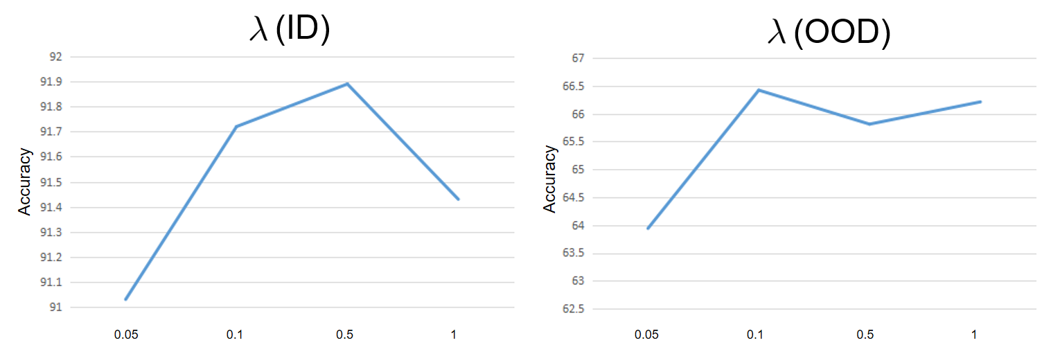
Ablation of .
We ablate in Figure.4(SM). The performances for in-distribution generalization is more robust than OOD generalization as varying .
Ablation of neural feature selector .
We provide the ablation about the role of neural feature selector in the performance boost. We train the IIL model as usual then test the model w/wo neural feature selector, respectively; and we also compare their results with their baseline InvRat. As observed in Table.5, the neural feature selector improve the performance literally based on . We also find that even if the feature selector is deactivated, trained by IIL remains superior than the original InvRat.
| w | wo | InvRat | |
|---|---|---|---|
| Accuracy (ID) | 91.72 | 90.34 | 89.25 |
| Accuracy (OOD, ) | 66.42 | 62.46 | 61.75 |
Ablation of .
We finally provide the ablation of executed by MINE technique. As viewed in Table.6, we find that the performance of IIL drop significantly without the MI maximization contraint. It is probably due to the trivial outcome generated by the joint CMI objective. It emphasizes the importance of preventing the trivial solution.
| Methods | InvRat (ID) | IIB (ID) | InvRat (OOD) | IIB (OOD) |
|---|---|---|---|---|
| wo | 90.15 | 91.74 | 64.26 | 67.89 |
| w | 91.72 | 93.17 | 66.42 | 69.59 |
Conclusion
This paper attempts to resolve the fake invariance problem for IRL, which undermines the OOD generalization performance. We proposes a novel structural causal model, ReStructured SCM (RS-SCM) to reconstruct both spurious and fake invariant features from the data. Our RS-SCM inspires a neural feature selection approach based on conditional mutual information to eliminate the spurious and fake invariant effects. Experiments demonstrates the effectiveness of our method on various OOD generalization benchmarks.
Appendix.A
The Derivation of “Spuriousness”
Here we demonstrate the derivation to induce the spuriousness property of invariant features. The equality in the second line is simply derived from MI’s chain rule and its rearrangement -, i.e.,
As for the inequality
in the third line, it can be achieved when the shortcut is considered as a part of the Markov chain given the Assumptions 1-3. Specifically, we have
Lemma 1.
Given the data generation processes defined by FIIF, PIIF, and RS-SCM Assumptions, the shortcut variable with the Markov dependency holds the inequality
Proof.
Notice that, the left side of the inequality holds
which can be derived from the steps of proving data processing inequality. We may derive the right side of the inequality by following a similar routine:
and with MI’s chain rule, we have
Combining the equations, the right term refers to
So the third-line inequality is equivalent with
We consider the Markov chain recovered by neural nets that reverses the data generation path in SCMs. , are independent given so that =. Then given as addition condition w.r.t. the SCMs that FIIF, PIIF, and RS-SCM Assumptions suit, the variables and are independent so that =. So we only need to justify . It can hold given and , which are both satisfied across the SCMs with the Markov chain (, in the first condition are directly related in the SCMs and for the second condition, since is a collider between and , conditioning blocks the only backdoor path from to , which further leads to the independence). ∎
We can simply obtain the third line from Lemma.1.
Proof of Proposition.1
Proof.
The first property of the fake invariant feature leads to . Given this, we consider the feature composed by and , i.e., , in which represents the variable of feature subset in (); denotes the variable of feature subset in (). Derived from the property of , it leads to due to composed by the invariant and fake invarint parts of . In terms of , it is also observed that
Therefore we have
The proposition has been proved. ∎
Proof of Proposition.2
Proof.
Suppose that and the variable denotes a subset of features recovered from . Given as the variable of feature subset in () and as the variable of feature subset in (), we consider four cases for : (1).;(2).;(3).;(4).. The final case is obviously impossible otherwise we obtain
which violates the condition given. The second case is also impossible since
In terms of and , it leads to
which also violates the condition given.
Here we focus on the third case. It can not assume otherwise
where leads to either
that violates the given condition with or
that violates the second property of with . In terms of and ,
obviously violates the given second condition also. To this, we only have and with
that suits the given condition. Finally, the first case leads to
which violates the given second condition. In terms of , there exists
obivously suiting the given condition also.
As discussed previously, we obtain the candidates and that both fulfill the propostion’s condition implied by the joint CMI objecitve. Whereas the trivial would dominate the objective since
| (10) | ||||
so that we incorporate
| (11) |
into the joint CMI objective that prevents the result from the trivial solution .
The proposition has been proven. ∎
Appendix.B
Our implementation is derived from the code /github.com/ Luodian/IIB/tree/IIB, by simply adding the joint CMI contraint and Eq.11 that jointly train our neural feature selector with feature encoder, invariant predictor and domain-aware predictor in IIB. More specifically, in our diagnostic experiments the architectures of feature encoder, invariant predictor and domain-aware predictor exactly follow the architecture used in their CS-MNIST experiment; similarly, our real-world experiment also follows their architecture setup used in the DomainBed experiments. In terms of our neural feature selector , our diagnostic experiments take a two-layer MLP architecture with a bottleneck (He et al. 2016), which follows the width size consistent to the second last layer of the feature encoder; our real-world experiments take a MAB architecture (Lee et al. 2019) with a single-head attention deployment. We incorporate the mutual information neural estimator (MINE) (Belghazi et al. 2018)(https://github.com/mohith-sakthivel/mine-pytorch) to achieve the MI maximization constraint (Eq.11) between and .
The inner loop training phase of IIL refers to the optimization of InvRat/ IIB based on the code /github.com/Luodian/ IIB/tree/IIB, wherein we follow their hyperparameter setup. In the outer loop, we set up across all experiments and use the same optimizer and hyperparameter in the inner loop. In the alternative phase, we employs the previous optimization setup both for the inner loop and outer loop, then after an outer loop epoch finishes, IIL alters to the inner loop to fine-tune the subnetworks with iterations until the in-distribution performance converges.
References
- Ahmed et al. (2020) Ahmed, F.; Bengio, Y.; Van Seijen, H.; and Courville, A. 2020. Systematic generalisation with group invariant predictions. In International Conference on Learning Representations.
- Ahuja et al. (2021) Ahuja, K.; Caballero, E.; Zhang, D.; Gagnon-Audet, J.-C.; Bengio, Y.; Mitliagkas, I.; and Rish, I. 2021. Invariance principle meets information bottleneck for out-of-distribution generalization. Advances in Neural Information Processing Systems, 34: 3438–3450.
- Ahuja et al. (2020) Ahuja, K.; Shanmugam, K.; Varshney, K.; and Dhurandhar, A. 2020. Invariant risk minimization games. In International Conference on Machine Learning, 145–155. PMLR.
- Alemi et al. (2016) Alemi, A. A.; Fischer, I.; Dillon, J. V.; and Murphy, K. 2016. Deep Variational Information Bottleneck. In International Conference on Learning Representations.
- Arjovsky et al. (2019) Arjovsky, M.; Bottou, L.; Gulrajani, I.; and Lopez-Paz, D. 2019. Invariant risk minimization. arXiv preprint arXiv:1907.02893.
- Belghazi et al. (2018) Belghazi, M. I.; Baratin, A.; Rajeshwar, S.; Ozair, S.; Bengio, Y.; Courville, A.; and Hjelm, D. 2018. Mutual information neural estimation. In International conference on machine learning, 531–540. PMLR.
- Chang et al. (2020) Chang, S.; Zhang, Y.; Yu, M.; and Jaakkola, T. 2020. Invariant rationalization. In International Conference on Machine Learning, 1448–1458. PMLR.
- Chen et al. (2023) Chen, J.; Gao, Z.; Wu, X.; and Luo, J. 2023. Meta-causal Learning for Single Domain Generalization. In Proceedings of the IEEE/CVF Conference on Computer Vision and Pattern Recognition, 7683–7692.
- Chen and Bühlmann (2021) Chen, Y.; and Bühlmann, P. 2021. Domain adaptation under structural causal models. The Journal of Machine Learning Research, 22(1): 11856–11935.
- Chevalley et al. (2022) Chevalley, M.; Bunne, C.; Krause, A.; and Bauer, S. 2022. Invariant causal mechanisms through distribution matching. arXiv preprint arXiv:2206.11646.
- Chu et al. (2022) Chu, X.; Jin, Y.; Zhu, W.; Wang, Y.; Wang, X.; Zhang, S.; and Mei, H. 2022. DNA: Domain generalization with diversified neural averaging. In International Conference on Machine Learning, 4010–4034. PMLR.
- Ganin et al. (2016) Ganin, Y.; Ustinova, E.; Ajakan, H.; Germain, P.; Larochelle, H.; Laviolette, F.; Marchand, M.; and Lempitsky, V. 2016. Domain-adversarial training of neural networks. The journal of machine learning research, 17(1): 2096–2030.
- Gulrajani and Lopez-Paz (2020) Gulrajani, I.; and Lopez-Paz, D. 2020. In search of lost domain generalization. arXiv preprint arXiv:2007.01434.
- He et al. (2016) He, K.; Zhang, X.; Ren, S.; and Sun, J. 2016. Deep residual learning for image recognition. In Proceedings of the IEEE conference on computer vision and pattern recognition, 770–778.
- Huh and Baidya (2022) Huh, D.; and Baidya, A. 2022. The Missing Invariance Principle found–the Reciprocal Twin of Invariant Risk Minimization. Advances in Neural Information Processing Systems, 35: 23023–23035.
- (16) Jalaldoust, K.; and Bareinboim, E. ???? Transportable Representations for Out-of-distribution Generalization.
- Jiang and Veitch (2022) Jiang, Y.; and Veitch, V. 2022. Invariant and transportable representations for anti-causal domain shifts. Advances in Neural Information Processing Systems, 35: 20782–20794.
- Kamath et al. (2021) Kamath, P.; Tangella, A.; Sutherland, D.; and Srebro, N. 2021. Does invariant risk minimization capture invariance? In International Conference on Artificial Intelligence and Statistics, 4069–4077. PMLR.
- Khirodkar, Yoo, and Kitani (2019) Khirodkar, R.; Yoo, D.; and Kitani, K. 2019. Domain randomization for scene-specific car detection and pose estimation. In 2019 IEEE Winter Conference on Applications of Computer Vision (WACV), 1932–1940. IEEE.
- Krueger et al. (2021) Krueger, D.; Caballero, E.; Jacobsen, J.-H.; Zhang, A.; Binas, J.; Zhang, D.; Le Priol, R.; and Courville, A. 2021. Out-of-distribution generalization via risk extrapolation (rex). In International Conference on Machine Learning, 5815–5826. PMLR.
- Kuang et al. (2018) Kuang, K.; Cui, P.; Athey, S.; Xiong, R.; and Li, B. 2018. Stable prediction across unknown environments. In proceedings of the 24th ACM SIGKDD international conference on knowledge discovery & data mining, 1617–1626.
- Lee et al. (2019) Lee, J.; Lee, Y.; Kim, J.; Kosiorek, A.; Choi, S.; and Teh, Y. W. 2019. Set transformer: A framework for attention-based permutation-invariant neural networks. In International conference on machine learning, 3744–3753. PMLR.
- Lee, Kim, and Kwak (2022) Lee, K.; Kim, S.; and Kwak, S. 2022. Cross-domain ensemble distillation for domain generalization. In European Conference on Computer Vision, 1–20. Springer.
- Li et al. (2022) Li, B.; Shen, Y.; Wang, Y.; Zhu, W.; Li, D.; Keutzer, K.; and Zhao, H. 2022. Invariant information bottleneck for domain generalization. In Proceedings of the AAAI Conference on Artificial Intelligence, volume 36, 7399–7407.
- Lin et al. (2022) Lin, Y.; Zhu, S.; Tan, L.; and Cui, P. 2022. ZIN: When and How to Learn Invariance Without Environment Partition? Advances in Neural Information Processing Systems, 35: 24529–24542.
- Lv et al. (2022) Lv, F.; Liang, J.; Li, S.; Zang, B.; Liu, C. H.; Wang, Z.; and Liu, D. 2022. Causality inspired representation learning for domain generalization. In Proceedings of the IEEE/CVF Conference on Computer Vision and Pattern Recognition, 8046–8056.
- Mahajan, Tople, and Sharma (2021) Mahajan, D.; Tople, S.; and Sharma, A. 2021. Domain generalization using causal matching. In International Conference on Machine Learning, 7313–7324. PMLR.
- Nagarajan, Andreassen, and Neyshabur (2020) Nagarajan, V.; Andreassen, A.; and Neyshabur, B. 2020. Understanding the failure modes of out-of-distribution generalization. In International Conference on Learning Representations.
- Pearl (2009) Pearl, J. 2009. Causal inference in statistics: An overview.
- Pearl (2010) Pearl, J. 2010. Causal inference. Causality: objectives and assessment, 39–58.
- Peters, Bühlmann, and Meinshausen (2016) Peters, J.; Bühlmann, P.; and Meinshausen, N. 2016. Causal inference by using invariant prediction: identification and confidence intervals. Journal of the Royal Statistical Society Series B: Statistical Methodology, 78(5): 947–1012.
- Rosenfeld, Ravikumar, and Risteski (2020) Rosenfeld, E.; Ravikumar, P. K.; and Risteski, A. 2020. The Risks of Invariant Risk Minimization. In International Conference on Learning Representations.
- Shen et al. (2021) Shen, Z.; Liu, J.; He, Y.; Zhang, X.; Xu, R.; Yu, H.; and Cui, P. 2021. Towards out-of-distribution generalization: A survey. arXiv preprint arXiv:2108.13624.
- Shu et al. (2021) Shu, Y.; Cao, Z.; Wang, C.; Wang, J.; and Long, M. 2021. Open domain generalization with domain-augmented meta-learning. In Proceedings of the IEEE/CVF conference on computer vision and pattern recognition, 9624–9633.
- Wang et al. (2022a) Wang, J.; Lan, C.; Liu, C.; Ouyang, Y.; Qin, T.; Lu, W.; Chen, Y.; Zeng, W.; and Yu, P. 2022a. Generalizing to unseen domains: A survey on domain generalization. IEEE Transactions on Knowledge and Data Engineering.
- Wang et al. (2022b) Wang, R.; Yi, M.; Chen, Z.; and Zhu, S. 2022b. Out-of-distribution generalization with causal invariant transformations. In Proceedings of the IEEE/CVF Conference on Computer Vision and Pattern Recognition, 375–385.
- Wang, Li, and Kot (2020) Wang, Y.; Li, H.; and Kot, A. C. 2020. Heterogeneous domain generalization via domain mixup. In ICASSP 2020-2020 IEEE International Conference on Acoustics, Speech and Signal Processing (ICASSP), 3622–3626. IEEE.
- Watson et al. (2023) Watson, R. A.; Cai, H.; An, X.; McLean, S.; and Song, R. 2023. On Heterogeneous Treatment Effects in Heterogeneous Causal Graphs. arXiv preprint arXiv:2301.12383.
- Yu et al. (2023) Yu, R.; Liu, S.; Yang, X.; and Wang, X. 2023. Distribution Shift Inversion for Out-of-Distribution Prediction. In Proceedings of the IEEE/CVF Conference on Computer Vision and Pattern Recognition, 3592–3602.
- Zhao et al. (2019) Zhao, H.; Des Combes, R. T.; Zhang, K.; and Gordon, G. 2019. On learning invariant representations for domain adaptation. In International conference on machine learning, 7523–7532. PMLR.
- Zhou et al. (2022) Zhou, X.; Lin, Y.; Zhang, W.; and Zhang, T. 2022. Sparse invariant risk minimization. In International Conference on Machine Learning, 27222–27244. PMLR.