DG-TTA: Out-of-domain medical image segmentation through Domain Generalization and Test-Time Adaptation

Abstract

Applying pre-trained medical segmentation models on out-of-domain images often yields predictions of insufficient quality. Several strategies have been proposed to maintain model performance, such as finetuning or unsupervised- and source-free domain adaptation. These strategies set restrictive requirements for data availability. In this study, we propose to combine domain generalization and test-time adaptation to create a highly effective approach for reusing pre-trained models in unseen target domains. Domain-generalized pre-training on source data is used to obtain the best initial performance in the target domain. We introduce the MIND descriptor previously used in image registration tasks as a further technique to achieve generalization and present superior performance for small-scale datasets compared to existing approaches. At test-time, high-quality segmentation for every single unseen scan is ensured by optimizing the model weights for consistency given different image augmentations. That way, our method enables separate use of source and target data and thus removes current data availability barriers. Moreover, the presented method is highly modular as it does not require specific model architectures or prior knowledge of involved domains and labels. We demonstrate this by integrating it into the nnUNet, which is currently the most popular and accurate framework for medical image segmentation. We employ multiple datasets covering abdominal, cardiac, and lumbar spine scans and compose several out-of-domain scenarios in this study. We demonstrate that our method, combined with pre-trained whole-body CT models, can effectively segment MR images with high accuracy in all of the aforementioned scenarios. Open-source code can be found here: https://github.com/multimodallearning/DG-TTA

Keywords Domain generalization $\cdot$ Domain-invariant descriptors $\cdot$ Test-time adaptation

1 Introduction

Medical image analysis, particularly medical image segmentation, has made a significant leap forward in recent years with deep learning. However, changes in data distribution introduced by different input modalities or devices can lead to errors in the performance of deep learning models [undef]. Since multiple imaging techniques are often required for disease identification and treatment planning, and MRI devices especially offer broad flexibility in adjusting acquisition parameters, access to all imaging domains is usually infeasible. Consequently, trained models may produce inaccurate results when encountering unseen, out-of-domain data (OOD) at test-time [undefa].

Supervised finetuning can be used as a workaround to retrain or finetune networks for the unseen domain. Still, it would, in turn, require curating and labelling data again, which is costly and time-consuming. The most frequently studied approach to overcome this effort is using unsupervised domain adaptation (UDA), which incorporates labeled source and unlabeled target data [undefb, undefc, undefc, undefd, undefe, undeff, undefg]. Accessing the source and target data jointly in UDA imposes a challenge since source data can be unavailable when privacy concerns or other regulations restrict its transfer. For these reasons, source-free domain adaptation (SFDA) accesses source and target data separately in successive steps [undefh, undefi, undefj, undefk, undefh]. Here, methods require retraining on data of the target distribution to adapt models to the target domain. However, the assumption that access to a broad target distribution is available is not always valid, and in addition to that, technical expertise is needed to retrain a model. In practice, a single out-of-domain data sample is usually given for which we want to obtain optimal results immediately. As this is the most realistic and practical scenario, we target it in this study, facing the most challenging data constraints. Two complementary paradigms exist to maximize the performance in such a limited case — domain generalization (DG), which optimizes the model performance for ‘any’ unseen out-of-distribution sample and test-time adaptation (TTA), which optimizes the model performance only for the sample in question. DG methods use source-only data and optimize the training routine to derive a powerful base model that is presumably stable even under input distribution shifts [undefl, undefm, undefn, undefo, undefp, undefq, undefr, undefs, undeft, undefu, undefv, undefw]. For these methods, the challenge arises in foreseeing the possible target domains. DG is an ultimate goal to achieve, but up to now, no universal solution that robustly works has been found. TTA, on the other hand, can be used to recover models that perform poorly while only accessing an unlabeled target image, as shown in many studies [undefx, undefy, undefz, undefaa, undefab, undefac, undefad, undefae, undefaf]. We argue that linking both approaches enables optimal separate use of source and target data where DG maximizes the base performance and TTA can further optimize the result. Numerous DG and TTA methods have been developed, but linking them together requires compatibility with the selected methods. This implies that requirements for specific models, architectural changes and complex training routines are unfavourable. Especially, adaptation approaches often require complex strategies and assumptions such as intertwined adaptation layers [undefad, undefae], indirect supervision tasks [undefag, undefaa, undefac], prior knowledge about label distributions [undefz] or assumptions on the distinctiveness of domains [undefg], which we also summarize in Sec. 2. Moreover, when we aim to generate a universal solution to segment medical images in out-of-domain settings, the flexible applicability of the method is essential. This applicability has been overlooked in previous studies, where methods were mostly applied in complex, scattered and separated frameworks. This is why we propose to employ DG-TTA, a minimally invasive approach integrated into the state-of-the-art nnUNet [undefah] framework in the next section.

1.1 Contribution

In this study, we consider out-of-domain segmentation across domains with minimum constraints on data availability: Given the source data only at training-time and only one target sample of an unknown domain at test-time later, we aim to achieve an optimal segmentation performance. This crucially enables out-of-the-box use of off-the-shelf pre-trained segmentation networks without further training and could be directly employed in clinical practice.

• We propose combining DG pre-training and TTA to achieve optimal performance with minimum data requirements (DG-TTA).

• We introduce using the MIND feature descriptor previously only applied in image registration tasks for DG pre-training and show superiority for small-scale datasets.

• We perform TTA with a lean self-supervision scheme previously seen in UDA/SFDA [undefg, undefai] but new in this context. We further avoid any other auxiliary optimization tasks and the need for prior assumptions.

• We show that high-quality predictions of medical images can be obtained out-of-the-box by combining our methodologies, the state-of-the-art nnUNet segmentation framework [undefah], and pre-trained TotalSegmentator CT models.

2 Related work

2.1 Unsupervised- and source-free domain adaptation

Unsupervised domain adaptation provides the benefit that no labels of the target domain must be available to adapt a model. Methods have been developed to translate input images for optimal fit for the trained model, such as generative adversarial approaches: In CycleGAN [undefc], unpaired image-to-image translation is performed using two mapping functions to map an image to another domain and vice-versa supervised by discriminator-based- and cycle- consistency losses. Later, CUT and FastCUT [undefd] were developed, optimizing an encoder-decoder structure to extract domain-invariant features and add domain-specific information in the decoding step. Adversely, in [undefg], the segmentation network is forced to produce domain-invariant features by reversing the gradients of a domain classifier. At the same time, the decision boundary of class predictions is optimized using a consistency soft Dice loss of augmented input samples. The authors present UDA approaches that work with multiple and even on a single target sample.

To further reduce the need to share source data, UDA was sought to be replaced by SFDA methods [undefj, undefh, undefi]. Here, a common approach is to leverage pseudo-labels generated by the non-adapted base model and refine them to supervise the model adaptation. In [undefi], estimated class centroids were used as a proxy, and pixel-level uncertainties were used to discard inaccuracies of pseudo labels. More complex proxy pseudo-supervision schemes exist, such as in [undefj], where three cascaded base model variants with differing fixed weights were combined. Another versatile approach for SFDA is the mean teacher paradigm [undefk], initially developed for classification scenarios where a moving average of the student model’s weights is used to update a teacher model. In [undefh], a consistency loss between a teacher and student network is used for target data to which flipping and random-noise perturbations were applied. To explicitly update weights related to the domain shift, the distance of the updated weights to the original weights is measured, and a predetermined percentage of the lowest weights, which might not correspond to the domain shift, is not updated. Not constrained to SFDA, mean teacher schemes can also be found in UDA scenarios [undefai]. The mentioned approaches in this section have in common that they set strong assumptions on data availability at the time of application — source data in the case of UDA and a broad spectrum of the target data distribution.

2.2 Domain generalization

DG techniques are applied during training on the source data and enhance the model’s out-of-domain performance. One way to improve generalization is to increase the data manifold, such as in [undefl], where 14 publicly available CT datasets were combined in training. Also, the explicit declaration of domains is possible: Multiple labeled source domains are used during training, incorporating a domain classifier that differentiates between the domains in [undefq]. The training of generalizing models has also been studied with limited, single-source data. This removes the burden of extensive data acquisition. However, model generalization then needs to be enforced otherwise, e.g., through artificially increasing the data by augmentation: Augmentations can comprise simple intensity-based modifications such as the application of random noise [undefaj], partial corruption of image areas such as in [undefm, undefv, undefw], or more sophisticated methods such as convolution-operations with randomly initialized weights [undefn, undefo]. Unlike handcrafted or random augmentations, differentiable augmentation schemes were used in adversarial settings, where the applied augmentation was optimized so that the trained network was encouraged to perform well under optimally difficult conditions [undefp, undefq]. Domain randomization [undefr] leverages a complete virtual simulation of input data to provide broadly varying data, removing the constraints on augmenting captured data samples, and was also successfully applied for medical image segmentation in [undefs]. DG can not only be achieved by increasing the data manifold but also by adapting training strategies: In [undeft, undefu], multiple tasks comprising image restoration, classification, and segmentation were used to form a more general understanding of the model’s underlying data correlations.

2.3 Test-time adaptation

!t

Figure 1: Core ideas of related work for TTA in medical image segmentation.  -colored components are optimized at training-time, belong to the training-routine or knowledge of the training data.  -colored components are optimized in a consecutive step on the training data.  -colored components are optimized at test-time through $\mathcal{L}_{TTA}$ loss terms. Shaded   -components are optimized during training and test-time adaptation. For a complete overview, please refer to the related works described in the text.

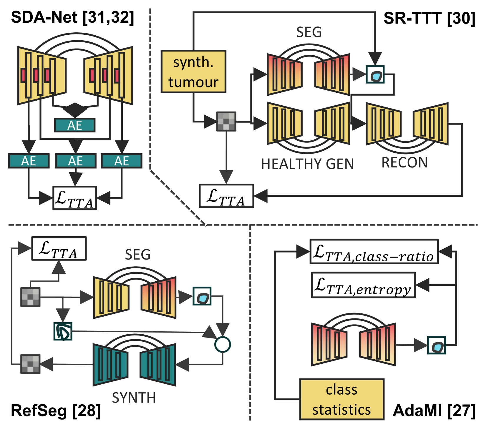
TTA operates in the target data domain and, as opposed to UDA and SFDA methods, only requires one single target sample for adaptation. Model adaptation can be driven by minimizing entropy-based measures [undefx, undefz] and the introduction of auxiliary tasks [undefy, undefab, undefac]. These concepts were applied multifaceted in medical imaging, as depicted in some selected works in Fig. 1.

In AdaMI [undefz], TTA is performed using a class-ratio prior and a mutual information-based entropy minimization of the predicted softmax output maps. More complex supervision schemes can be found in RefSeg [undefaa], where a framework iteratively improves predictions by synthesizing input images from edge-maps and segmentation heatmaps. The synthesized images are supervised using normalized cross-correlation and MI-based loss functions. A denoising autoencoder is used in [undefab] to fix implausible segmentation output by the base segmentation network. An image normalization layer is then adapted to provide correctly normalized input for the segmentation model by supervising it with the denoised pseudo-label. In SR-TTT, a two-task training routine is employed [undefac]: Healthy images are generated from hand-crafted, synthesized liver tumor images. A subsequent segmentation network predicts tumor masks and a third reconstruction network uses masks and healthy images to synthesize tumor images, forming a closed loop for TTA. Instead of entropy-based losses SDA-Net [undefad, undefae] uses several autoencoder-based losses to measure the feature discrepancy of target samples. The architecture consists of a U-Net with specific intertwined layers for adaptation. Apart from the indirect supervision of pseudo-targets, consistency schemes are also successfully applied: In [undefaf], coefficients for a linear combination of fixed shape dictionary items are learned. During TTA, these coefficients are predicted for noise-perturbed input samples, and the consistency of shape coefficients and final segmentations is measured.

3 Methodology

As shown in Fig. 2, we split our method into two parts: Firstly, the model training takes place on the source domain data by minimizing cross-entropy and Dice loss terms [undefah]. We propose doing this with the DG techniques described below to prepare the model for prediction in out-of-domain scenarios. Secondly, our TTA strategy is employed on individual target domain samples after model training.

Figure 2: Left: Model pre-training with source domain data. We propose to use GIN, MIND or their combination GIN+MIND in this step. Right: DG-TTA method applied in the target data domain. Two differently augmented versions of the same input are passed through the pre-trained segmentation network. The network weights are then optimized supervising the predictions with a Dice loss steering the network to produce consistent predictions.

3.1 DG pre-training

Pre-training is performed on the labeled source training dataset $D_{train}=\{\mathbf{x_{s}},\mathbf{y_{s}}\}_{s=1}^{l}$, $l\in\mathbb{N}^{+}$, where $\mathbf{x_{s}}$ and $\mathbf{y_{s}}$ can also be patches. Recently, global intensity non-linear augmentation GIN [undefo] was introduced to improve model generalization during training. In GIN, a shallow convolutional network with LeakyReLU nonlinearities $g$ is re-initialized at each iteration by random parameters $\rho$ and used to augment the input $\mathbf{x}$. The augmented image is then blended with the original image weighted by $\alpha$:

$$\text{GIN}(\mathbf{x})=\alpha\,g_{\rho}(\mathbf{x})+(1-\alpha)\,\mathbf{x}$$ (1)

We propose using MIND descriptors [undefak] as a promising alternative to GIN. In contrast to GIN, it provides handcrafted features from the input to derive a modality- and contrast-independent representation:

$$\text{MIND}(\mathbf{x,p,d})=\text{exp}\left(-\frac{SSD(\mathbf{x},\mathbf{p},\mathbf{d})}{\sigma^{2}_{\mathcal{N}}}\right),\quad\mathbf{p,d}\in\mathcal{N}$$ (2)

For a given image/patch $\mathbf{x}$, sub-blocks (small patches) at location $\mathbf{p}$ are extracted, and their sum of squared distances (SSD) to neighboring blocks at distance $\mathbf{d}$ are evaluated. This difference is weighted by a local variance estimate $\sigma_{\mathcal{N}}$, more specifically, the mean of all block differences according to the method. The neighborhood $\mathcal{N}$ is defined as all diagonally adjacent blocks of the 6-neighborhood around the center block at $p$ resulting in a mapping of $\mathbb{R}^{1\times\lvert\Omega\rvert}\to\mathbb{R}^{12\times\lvert\Omega\rvert}$ for voxel space $\Omega$. Note that for inference or testing, the MIND descriptor is always applied to provide the correct number of input channels to the network. For DG, we also propose using the combination of both methods, where before applying the MIND descriptor, the input is augmented using GIN (MIND+GIN).

3.2 TTA

Our test-time adaptation method can now be applied to pre-trained models: For any given pre-trained model $f_{\theta}$ on the training dataset $D_{train}$, we want to adjust the weights optimally to a single unseen sample of the target test set $D_{test}=\{\mathbf{x_{t}}\}$ during TTA.

Instead of adding additional supervision tasks and complex architectures, we propose to use two augmentations, $A$ and $B$, to obtain differently augmented images. The core idea of the method is to optimize the network to produce consistent predictions given two differently augmented inputs, where $S_{A/B}$ each denote spatial augmentation:

$$\mathbf{x_{A,t}} =A(\mathbf{x_{t}}),\quad A=S_{A} \quad A:\mathbb{R}^{\lvert\Omega\rvert}\rightarrow\mathbb{R}^{\lvert\Omega\rvert}$$ (3)

$$\mathbf{x_{B,t}} =B(\mathbf{x_{t}}),\quad B=S_{B} \quad B:\mathbb{R}^{\lvert\Omega\rvert}\rightarrow\mathbb{R}^{\lvert\Omega\rvert}$$ (4)

Both augmented images are passed through the pre-trained network $f_{\theta}$:

$$\mathbf{\hat{y}_{A/B,t}}=f_{\theta}(\mathbf{x_{A/B,t}})$$ (5)

Prior to calculating the consistency loss, both predictions $\mathbf{\hat{y}_{A/B,t}}$ need to be mapped back to the initial spatial orientation for voxel-wise compatibility by applying the inverse transformation operation $S_{A/B}^{-1}$. In addition, a consistency masking $m_{c}(\cdot)$ is applied to filter inversion artifacts with $\zeta$ indicating voxels that were introduced at the image borders during the inverse spatial transformation but are unrelated to the original image content:

$$m_{c}(\mathbf{\hat{y}_{A}},\mathbf{\hat{y}_{B}}) =\left[\mathbf{\hat{y}_{A}}\neq\zeta\right]\wedge\left[\mathbf{\hat{y}_{B}}\neq\zeta\right]$$ (6)

$$A^{-1} =m_{c}\circ S_{A}^{-1}$$ (7)

$$B^{-1} =m_{c}\circ S_{B}^{-1}$$ (8)

Figure 3: Dice loss landscapes and values for $d=[1,2]$ in Eq. 10. $d=2$ yields zero loss along the diagonal, which is favorable for consistency.

We steer the network to produce consistent outputs by comparing them after inversion and masking:

$$\mathcal{L}_{TTA}=\ell\left(A^{-1}\circ f_{\theta}\left(\mathbf{x_{A,t}}\right),B^{-1}\circ f_{\theta}\left(\mathbf{x_{B,t}}\right)\right)$$ (9)

As loss function $\ell$, we choose a Dice loss with predictions $\mathbf{\hat{y}_{A}}$ and $\mathbf{\hat{y}_{B}}$ given as class probabilities for all voxels in $\Omega$:

$$\ell(\mathbf{\hat{y}_{A}},\mathbf{\hat{y}_{B}})=\frac{1}{\lvert\Omega\rvert}\sum_{\omega}^{\Omega}\frac{2\cdot\hat{y}_{A,\omega}\cdot\hat{y}_{B,\omega}}{{\hat{y}_{A,\omega}}^{d}+{\hat{y}_{B,\omega}}^{d}}$$ (10)

Selecting $d=2$ ensures consistency in the Dice loss landscape instead of $d=1$, which forces the network to additionally maximize the confidence of the prediction (see Fig. 3).

3.3 Spatial augmentation

For spatial augmentation, we use affine image distortions on image/patch coordinates $\mathbf{c_{x}}$:

$$\phi(\mathbf{c_{x}})=\mathbf{Mc_{x}},\quad\mathbf{M}=\begin{pmatrix}r_{11}&r_{12}&r_{13}&t_{14}\\ r_{21}&r_{22}&r_{23}&t_{24}\\ r_{31}&r_{32}&r_{33}&t_{34}\\ 0&0&0&1\end{pmatrix}$$ (11)

The submatrix $\mathbf{R}$ contains only rotational components $r_{11}\dots r_{33}$ such that $\mathbf{R}\mathbf{R^{T}}=\mathbb{1}$. For the inverse transformation $\mathbf{M}^{-1}$ is used. Although we describe only affine spatial augmentation in this section and Fig. 2, we also explored B-spline spatial- and intensity augmentation in various combinations during TTA. However, we found affine spatial augmentation on its own to be most effective.

3.4 Optimization strategy

During TTA, only the classes of interest are optimized, meaning that we omit all other classes of the predictions $\mathbf{\hat{y}_{A}}$ and $\mathbf{\hat{y}_{B}}$ for supervision: e.g. in Experiment III in the abdominal TTA scenario, all abdominal classes are supervised, but we omit cardiac, spine, lung and other irrelevant classes from the TS base model (see Sec. 4.1.5). To increase the robustness of predicted labels, we use an ensemble of three TTA models in the final inference routine of the nnUNet framework [undefah]. All models were optimized with the AdamW optimizer with a learning rate of $\eta=1e{-5}$, weight decay $\beta=0.01$, and no scheduling for twelve epochs. In former experiments, we identified that special caution has to be taken when applying test-time adaptation to models that require patch-based input. Since patch-based inference limits the field of view, the optimizer will adapt the model weights and overfit for consistency of the specific image region. Therefore, we accumulate gradients of $N_{p}=16$ randomly drawn patches during one epoch prior to taking an optimization step to fit GPU memory limits.

4 Experiments

Experiment I: We perform an extensive evaluation of models with and without DG capabilities predicting across the domain gap between CT $\mathrel{\hbox{\rule[2.3pt]{3.0pt}{0.4pt}}\mkern-4.0mu\hbox{\char 41\relax}}$ MR and MR $\mathrel{\hbox{\rule[2.3pt]{3.0pt}{0.4pt}}\mkern-4.0mu\hbox{\char 41\relax}}$ CT and report the associated gaps in accuracy compared to models that have been trained in the target domain. Experiment II: TTA is then applied for CT $\mathrel{\hbox{\rule[2.3pt]{3.0pt}{0.4pt}}\mkern-4.0mu\hbox{\char 41\relax}}$ MR prediction to show the potential of recovering model performance. We compare our method to a subset of related TTA approaches (see Sec. 2). Experiment III: We provide results on various out-of-domain segmentation scenarios to further broaden our study.

4.1 Datasets

4.1.1 BTCV: Multi-Atlas Labeling Beyond the Cranial Vault

The dataset [undefal] contains 30 labeled abdominal CT scans of a colorectal cancer chemotherapy trial with 14 organs: Spleen (SPL), right kidney (RKN), left kidney (LKN), gallbladder (GAL), esophagus (ESO), liver (LIV), stomach (STO), aorta (AO), inferior vena cava (IVC), portal vein and splenic vein (PSV), pancreas (PAN), right adrenal gland (RAG) and left adrenal gland (LAG). Data dimensions reach from $512\text{\,}\mathrm{}$$\times$$512\text{\,}\mathrm{}$$\times$$85\text{\,}\mathrm{vox}$ to $512\text{\,}\mathrm{}$$\times$$512\text{\,}\mathrm{}$$\times$$198\text{\,}\mathrm{vox}$ and fields of view from $280\text{\,}\mathrm{}$$\times$$280\text{\,}\mathrm{}$$\times$$280\text{\,}{\mathrm{mm}}^{3}$ to $500\text{\,}\mathrm{}$$\times$$500\text{\,}\mathrm{}$$\times$$650\text{\,}{\mathrm{mm}}^{3}$. We split the dataset into a 20/10 training/test set for our experiments and use a subset of ten classes that are uniformly labeled in all scans.

4.1.2 AMOS: A Large-Scale Abdominal Multi-Organ Benchmark for Versatile Medical Image Segmentation

The AMOS dataset [undefam] consists of CT and MRI scans from eight scanners with a similar field of view as the BTCV dataset of patients with structural abnormalities in the abdominal region (tumors, etc.). Unlike the BTCV dataset’s organs, AMOS has additional segmentation labels for the duodenum, bladder, and prostate/uterus but not for the PSV class. We used 40 of the labeled images (MR only, axial resolution $0.82\text{\,}\mathrm{}$ up to $3.00\text{\,}\mathrm{mm}$) and split them into 30/10 training/testing samples so that the number of test samples is comparable to the BTCV dataset.

4.1.3 MMWHS: Multi-Modality Whole Heart Segmentation

This dataset [undefan] contains CT and MR images of seven cardiac structures: Left ventricle, right ventricle, left atrium, right atrium, the myocardium of left ventricle, ascending aorta, and pulmonary artery. The CT data resolution is $0.78\text{\,}\mathrm{}$$\times$$0.78\text{\,}\mathrm{}$$\times$$0.78\text{\,}{\mathrm{mm}}^{3}\text{/}\mathrm{vox}$. The cardiac MRI data was obtained from two sites with a 1.5 T scanner and reconstructed to obtain resolutions from $0.80\text{\,}\mathrm{}$$\times$$0.80\text{\,}\mathrm{}$$\times$$1.00\text{\,}{\mathrm{mm}}^{3}\text{/}\mathrm{vox}$ down to $1.00\text{\,}\mathrm{}$$\times$$1.00\text{\,}\mathrm{}$$\times$$1.60\text{\,}{\mathrm{mm}}^{3}\text{/}\mathrm{vox}$. We split the labeled 20 CT and 20 MR images into 16/4 training/testing cases.

4.1.4 SPINE: MyoSegmenTUM spine

This MRI dataset [undefao] contains water, fat, and proton density-weighted lumbal spine scans with manually labeled vertebral bodies L1 — L5. The field of view spans $220\text{\,}\mathrm{}$$\times$$220\text{\,}\mathrm{}$$\times$$80\text{\,}{\mathrm{mm}}^{3}$ with a resolution of $1.8\text{\,}\mathrm{}$$\times$$1.8\text{\,}\mathrm{}$$\times$$4.0\text{\,}{\mathrm{mm}}^{3}\text{/}\mathrm{vox}$.

4.1.5 TS: TotalSegmentator, 104 labels

The large-scale TS dataset contains CT images of 1204 subjects with 104 annotated classes. The annotations were created semi-automated, where a clinician checked every annotation. The data was acquired across eight sites on 16 scanners with varying slice thickness and resolution [undefap]. Differing from the SPINE dataset, the vertebral bodies and the spinous processes are included in the class labels of this dataset, and intermediate model predictions were corrected accordingly in a postprocessing step to obtain reasonable results for evaluation.

4.1.6 Pre-/postprocessing

We resampled all datasets to a uniform voxel size of $1.50\text{\,}\mathrm{}$$\times$$1.50\text{\,}\mathrm{}$$\times$$1.50\text{\,}{\mathrm{mm}}^{3}\text{/}\mathrm{vox}$. For the SPINE task, we cropped the TS ground truth to omit the spinous processes with a mask dilated five voxels around the proposed prediction in the TS $\mathrel{\hbox{\rule[2.3pt]{3.0pt}{0.4pt}}\mkern-4.0mu\hbox{\char 41\relax}}$ SPINE out-of-domain prediction setting to provide comparable annotations (see Sec. 4.2.3).

4.2 Experiment structure

4.2.1 Experiment I: Domain gap evaluation of non-DG and DG pre-trained models

The two abdominal datasets, AMOS (MR) and BTCV (CT), are used in this experiment to evaluate out-of-domain gaps of multiple models. More specifically, we evaluate the performance of eight different segmentation models (one 2D model and seven 3D models), all trained in the unified nnUNet framework [undefah]. Three models were pre-trained without explicit domain generalization techniques: A 2D nnUNet model (NNUNET 2D) to show the difference of 2D and 3D performance, a 3D nnUNet model (NNUNET) and a 3D nnUNet model with Batch Normalization layers (NNUNET BN) instead of Instance Normalization layers. Five models were pre-trained with domain generalization techniques targeting the input data augmentation: A nnUNet model with extensive spatial and intensity augmentation (INSANE DA), checkerboard masked images with a dropout rate of 30% (MIC, [undefw]), GIN intensity augmentation (see Sec. 3 and [undefo, undefn]), the MIND descriptor (see Sec. 3 and [undefak]) and a combination of GIN and MIND (GIN+MIND). All sub-experiments were conducted in two ways: Training on the CT data and testing on the MR data CT $\mathrel{\hbox{\rule[2.3pt]{3.0pt}{0.4pt}}\mkern-4.0mu\hbox{\char 41\relax}}$ MR and vice-versa MR $\mathrel{\hbox{\rule[2.3pt]{3.0pt}{0.4pt}}\mkern-4.0mu\hbox{\char 41\relax}}$ CT.

4.2.2 Experiment II: Performance evaluation of DG-TTA

This experiment aims to show the potential of our TTA approach subsequently applied to pre-trained models. We evaluate the performance of our and two competing TTA approaches AdaMI and SDA-Net (see Sec. 2), selecting the competing approaches that share an essential benefit with our proposed DG-TTA method that no additional complex generative supervision tasks are necessary. For AdaMI, a class ratio prior needs to be provided, which we estimate by averaging class voxel counts of the training dataset while we consider the same field of view of the drawn TTA patch.

4.2.3 Experiment III: High quality predictions on unseen data out-of-the-box: More scenarios

Building upon Experiment II, we show efficacy of our method leveraging the TS dataset with 104 labels as a strong basis in three segmentation tasks (all CT $\mathrel{\hbox{\rule[2.3pt]{3.0pt}{0.4pt}}\mkern-4.0mu\hbox{\char 41\relax}}$ MR): Abdominal organ-(TS $\mathrel{\hbox{\rule[2.3pt]{3.0pt}{0.4pt}}\mkern-4.0mu\hbox{\char 41\relax}}$ AMOS), lumbal spine- (TS $\mathrel{\hbox{\rule[2.3pt]{3.0pt}{0.4pt}}\mkern-4.0mu\hbox{\char 41\relax}}$ SPINE) and whole-heart segmentation (TS $\mathrel{\hbox{\rule[2.3pt]{3.0pt}{0.4pt}}\mkern-4.0mu\hbox{\char 41\relax}}$ MMWHS MR). Furthermore, we present results for whole-heart segmentation using only models pre-trained with as few as 16 CT samples in MMWHS CT $\mathrel{\hbox{\rule[2.3pt]{3.0pt}{0.4pt}}\mkern-4.0mu\hbox{\char 41\relax}}$ MMWHS MR.

5 Results

In the following sections, segmentation quality is evaluated using the Dice score overlap metric. The significance of TTA improvements is determined with the one-sided Wilcoxon Signed Rank test [undefaq].

5.1 Experiment I: Domain gap evaluation of non-DG and DG pre-trained models

Figure 4: Evaluation of non-DG and DG pre-trained models in out-of-domain prediction scenarios. Dice scores reported of the in-domain prediction (upper baseline, - - -) and model performance in either MR $\mathrel{\hbox{\rule[2.3pt]{3.0pt}{0.4pt}}\mkern-4.0mu\hbox{\char 41\relax}}$ CT   or CT $\mathrel{\hbox{\rule[2.3pt]{3.0pt}{0.4pt}}\mkern-4.0mu\hbox{\char 41\relax}}$ MR   out-of-domain scenarios. Detailed gap scores of  -colored bars see Tab. 1

Table 1: Evaluation of models in CT $\mathrel{\hbox{\rule[2.3pt]{3.0pt}{0.4pt}}\mkern-4.0mu\hbox{\char 41\relax}}$ MR out-of-domain prediction for abdominal segmentation tasks (pre-training models on the BTCV dataset and testing on the AMOS dataset). This table shows detailed results  -colored bars of Fig. 4. Full class names can be found in Sec. 4.1.1

	MRI ID	MRI OOD (Dice %)
Pre-trained model	$\mu$		SPL	RKN	LKN	GAL	ESO	LIV	STO	AOR	IVC	PAN	$\mu\pm\sigma$	gap
NNUNET 2D	$78.8$		$14.1$	$3.0$	$2.0$	$2.0$	$4.5$	$15.2$	$0.1$	$10.1$	$2.8$	$0.8$	$5.5$ p m 11.2	$-73.3$
NNUNET	$84.5$		$40.2$	$21.9$	$15.9$	$24.9$	$22.9$	$76.0$	$34.3$	$26.4$	$21.8$	$35.3$	$32.0$ p m 27.6	$-52.6$
NNUNET BN	$84.3$		$0.0$	$0.0$	$0.0$	$0.0$	$0.3$	$43.7$	$0.0$	$2.3$	$0.5$	$1.5$	$4.9$ p m 15.6	$-79.4$
INSANE DA	$84.6$		$45.3$	$64.0$	$49.1$	$20.2$	$27.3$	$71.0$	$43.0$	$44.4$	$22.8$	$40.4$	$42.7$ p m 30.7	$-40.0$
MIC	$84.2$		$0.6$	$0.3$	$1.1$	$2.4$	$3.0$	$23.5$	$0.0$	$9.6$	$6.0$	$3.5$	$5.0$ p m 11.5	$-79.2$
GIN	$84.8$		$81.9$	$90.4$	$91.9$	$63.7$	$47.8$	$92.7$	$73.2$	$80.9$	$72.1$	$68.1$	$76.3$ p m 21.5	$-8.5$
MIND	$85.4$		$83.6$	$92.9$	$93.0$	$60.5$	$39.1$	$93.1$	$74.6$	$81.1$	$69.5$	$73.2$	$76.1$ p m 24.0	$-9.3$
GIN + MIND	$84.1$		$83.0$	93.3	93.3	65.9	50.3	94.1	76.5	83.9	73.7	$71.9$	$78.6$ p m 20.7	$-5.5$

Prediction across the CT $\mathrel{\hbox{\rule[2.3pt]{3.0pt}{0.4pt}}\mkern-4.0mu\hbox{\char 41\relax}}$ MR domain gap in the abdominal task of this experiment reveals that models behave differently depending on the model layer configuration and pre-training strategy (see Fig. 4): As expected, the 2D model achieves lower in-domain scores compared to 3D models. For seven of eight models, the domain gap from CT $\mathrel{\hbox{\rule[2.3pt]{3.0pt}{0.4pt}}\mkern-4.0mu\hbox{\char 41\relax}}$ MR is more challenging to compensate for, resulting in lower scores during out-of-domain testing. We focus on this domain gap in the following subexperiments and discussions. Inference of pre-trained models without generalization techniques results in severe gaps of $-52.6\text{\,}\mathrm{\char 37\relax}$ and $-79.4\text{\,}\mathrm{\char 37\relax}$ Dice when predicting in the MRI target domain (see Fig. 4 and Tab. 1). Increasing the data augmentation strength of the framework (INSANE DA) can reduce the gap to $-40.0\text{\,}\mathrm{\char 37\relax}$ Dice. Using techniques specifically designed for DG proves to be more effective: MIC [undefw] reduces the gap in the MR $\mathrel{\hbox{\rule[2.3pt]{3.0pt}{0.4pt}}\mkern-4.0mu\hbox{\char 41\relax}}$ CT scenario successfully, but we found it to be not as effective for the CT $\mathrel{\hbox{\rule[2.3pt]{3.0pt}{0.4pt}}\mkern-4.0mu\hbox{\char 41\relax}}$ MR scenario. GIN augmentation [undefo] and the MIND descriptor layer [undefak] significantly reduce the gap to ($-8.5\text{\,}\mathrm{}$/$-9.3\text{\,}\mathrm{\char 37\relax}$ Dice). Combining GIN+MIND results is the best strategy diminishing the gap to only $-5.5\text{\,}\mathrm{\char 37\relax}$ Dice. In detail, using the GIN+MIND combination resulted in the highest scores for segmentation in eight of ten abdominal organs (see Tab. 1).

5.2 Experiment II: Performance evaluation of DG-TTA

Figure 5: Test sample statistics before and after applying TTA (three of five models were pre-trained with DG techniques). For the NNUNET BN model, additionally, only the Batch Normalisation layers (nor) or only the encoder (enc) parameters were adapted. Results for three of five SDA-Net runs excluded due to collapsing predictions. Scores for individual classes can be found in Tab. 2 for DG-TTA, AdaMI and SDA-Net. Ordinate shows Dice scores in %. Median (-), mean (+) and the change in mean scores ($\rightarrow$) is depicted for boxes. Significance of improvement is shown above boxes (^*p<0.05; ^**p<0.01; ^***p<0.001).

Table 2: Evaluation of TTA methods for CT $\mathrel{\hbox{\rule[2.3pt]{3.0pt}{0.4pt}}\mkern-4.0mu\hbox{\char 41\relax}}$ MR test-time adaptation for the abdominal segmentation task (see Sec. 4.2.1 and Tab. 1). The class names are in Sec. 4.1.1. Bold scores indicate a per-model increase in scores, taking the scores of the non-adapted models of Tab. 1 into account. Results for three of five SDA-Net runs excluded due to collapsing predictions.

Pre-trained model	TTA method		SPL	RKN	LKN	GAL	ESO	LIV	STO	AOR	IVC	PAN	$\mu\pm\sigma$	gain
NNUNET	Ours		$76.0$	$70.0$	$74.4$	$42.5$	$42.0$	$79.8$	$52.0$	$65.2$	$46.7$	$60.8$	$60.9$ p m 25	$28.9$
	AdaMI		$75.0$	$77.7$	$83.1$	$37.1$	$37.9$	$83.8$	$56.5$	$68.1$	$48.2$	$61.1$	$62.8$ p m 25.3	$30.9$
	SDA-Net		$0.0$	$8.1$	$3.6$	$7.9$	$0.3$	$43.1$	$2.5$	$4.8$	$1.4$	$9.3$	$8.2$ p m 17.1	$-23.8$
NNUNET BN	Ours		$81.6$	$87.2$	$89.2$	$40.1$	$35.9$	$84.7$	$73.4$	$75.1$	$54.1$	$66.8$	$68.8$ p m 26.6	$63.9$
	AdaMI		$88.3$	$88.3$	$90.5$	$34.2$	$30.9$	$94.0$	$72.5$	$68.3$	$45.1$	$63.6$	$67.4$ p m 27.9	$62.4$
GIN	Ours		$81.6$	$90.5$	$92.1$	$72.3$	$48.9$	$93.3$	$74.7$	$79.2$	$70.9$	$70.6$	$77.4$ p m 19.8	$1.1$
	AdaMI		$78.5$	$86.6$	$90.9$	$71.1$	$47.2$	$92.2$	$69.0$	$78.3$	$68.4$	$66.9$	$74.9$ p m 20.0	$-1.4$
	SDA-Net		$70.9$	$86.8$	$86.9$	$60.6$	$41.6$	$89.4$	$69.3$	$74.2$	$65.6$	$54.4$	$70.0$ p m 24.4	$-6.3$
MIND	Ours		$83.4$	$91.2$	$92.9$	$68.1$	$48.6$	$91.4$	$74.4$	$83.3$	$71.3$	$72.2$	$77.7$ p m 21.4	$1.6$
	AdaMI		$81.1$	$92.4$	$92.5$	$69.7$	$41.7$	$92.7$	$72.6$	$80.7$	$69.5$	$72.9$	$76.6$ p m 21.7	$0.5$
GIN+MIND	Ours		$82.2$	$92.7$	$92.7$	$68.4$	$47.1$	$93.4$	$74.5$	$84.8$	$73.5$	$72.5$	$78.2$ p m 20.7	$-0.4$
	AdaMI		$79.4$	$91.5$	$92.6$	$70.5$	$47.9$	$91.9$	$73.5$	$80.7$	$72.3$	$70.8$	$77.1$ p m 20	$-1.5$

In preliminary combinatorial experiments, we found DG-TTA using gradients and backpropagation only in branch A and affine spatial augmentation in branches A and B to be an optimal tradeoff between non-DG- and DG pre-trained models. Note that we do not apply intensity augmentation, which proved counterproductive for DG pre-trained models. These settings will be used in the following experiments.

DG-TTA and AdaMI can recover prediction scores on non-DG pre-trained models by a large margin with significant improvements ($p<0.001$) as it can be seen in Fig. 5, left and Tab. 2: AdaMI reaches a top mean Dice of $62.8\text{\,}\mathrm{\char 37\relax}$ ($+30.9\text{\,}\mathrm{\char 37\relax}$) Dice for the pre-trained NNUNET model. DG-TTA reaches a top mean Dice of $68.8\text{\,}\mathrm{\char 37\relax}$ ($+63.9\text{\,}\mathrm{\char 37\relax}$) for NNUNET BN, which is remarkable comparing the scores to the low out-of-domain performance of the non-adapted model ($4.9\text{\,}\mathrm{\char 37\relax}$). As a further ablation, we report scores when only training the Batch Normalisation layers of NNUNET BN and for only training the encoder and found the best results when training all model parameters during TTA. Evaluating DG pre-trained models, DG-TTA improves GIN ($+1.1\text{\,}\mathrm{\char 37\relax}$) and MIND ($+1.6\text{\,}\mathrm{\char 37\relax}$) model outcomes. Applied to the GIN+MIND model, the Dice score decreases slightly ($-0.4\text{\,}\mathrm{\char 37\relax}$). AdaMI improves outcomes in the case of the MIND pre-trained model ($+0.5\text{\,}\mathrm{\char 37\relax}$) but does not reach the performance of our proposed method. We can show the superiority of our approach over the competing methods for four of five adapted models. The tested TTA methods for DG pre-trained models did not lead to statistically significant improvements, given that outcomes were already quite comparable to the in-domain performance.

Despite thorough finetuning and valid decreasing epoch loss values during TTA, we could not successfully apply SDA-Net in this 3D scenario and found scores to be collapsing by a large margin for most of the pre-trained models.

5.3 Experiment III: High quality predictions on unseen data out-of-the-box: More scenarios

Figure 6: Visual results correspond to statistics of Fig. 8 and 8. Rows show source and target task scenarios; columns indicate the base models used. Ground truth is given in the left column. Positively predicted voxels are shown in colors. The erroneous area of predictions is marked with contours. Class colors for the abdominal task can be found in Tab. 1. Whole-heart class labels comprise right ventricle  , right atrium  , left ventricle  , left atrium   and myocardium  . Best viewed digitally.

Figure 7: Test sample statistics before and after applying DG-TTA. Top: Abdominal organ prediction task of Exp. II. Bottom: Lumbal spine tasks. Symbols and axes description see Fig. 5.

Figure 8: Test sample statistics before and after applying DG-TTA for whole heart segmentation tasks. Top: TS pre-trained models. Bottom: MMWHS CT pre-trained models with only 16 training samples. Symbols and axes description see Fig. 5.

Now, we target prediction with DG-TTA in various tasks using the TS dataset as a basis since it contains 104 classes, making it a versatile starting point. The test prediction statistics are shown in Fig. 8 and Fig. 8. Again, DG pre-trained models perform strongly in the AMOS abdominal target task. The highest mean value of $82.6\text{\,}\mathrm{\char 37\relax}$ Dice can be achieved by applying DG-TTA on the GIN base model (see Fig. 8, top). This diminishes the domain gap to only $-2.2\text{\,}\mathrm{\char 37\relax}$ compared to the MRI in-domain prediction of $84.8\text{\,}\mathrm{\char 37\relax}$ (see Tab. 1). Out-of-domain prediction in the lumbal spine task TS $\mathrel{\hbox{\rule[2.3pt]{3.0pt}{0.4pt}}\mkern-4.0mu\hbox{\char 41\relax}}$ SPINE is challenging. Without TTA, only the pre-trained GIN model can reach a high performance of $73.2\text{\,}\mathrm{\char 37\relax}$. Applying DG-TTA on the GIN+MIND model leads to recovering the model’s capabilities to the highest test score of $73.7\text{\,}\mathrm{\char 37\relax}$ ($+15.8\text{\,}\mathrm{\char 37\relax}$). Out-of-domain prediction in the whole-heart segmentation tasks is performed well by DG pre-trained models on the TS dataset (see Fig. 8, top). The strong GIN model performance can be increased to $82.6\text{\,}\mathrm{\char 37\relax}$ Dice after applying TTA ($+1.2\text{\,}\mathrm{\char 37\relax}$).

With fewer training samples in the MMWHS CT $\mathrel{\hbox{\rule[2.3pt]{3.0pt}{0.4pt}}\mkern-4.0mu\hbox{\char 41\relax}}$ MR whole-heart segmentation tasks, lower scores are reported compared to the TS base model (see Fig. 8, bottom). Applying DG-TTA in such a challenging scenario can improve scores for all DG pre-trained models significantly ($+12.8\text{\,}\mathrm{\char 37\relax}$, $+11.8\text{\,}\mathrm{\char 37\relax}$, $+11.6\text{\,}\mathrm{\char 37\relax}$). Here, GIN+MIND reaches the best mean of 71.5 % Dice. Visual results of this experiment are depicted in Fig. 6.

6 Discussion and outlook

Severe domain shifts in medical imaging currently still prevent the reuse of segmentation models on newly acquired data. It is impossible to estimate a priori whether a pre-trained model with or without DG capabilities functions well out-of-domain. At the time of prediction, the source data might not be available anymore, disclosed due to regulatory limitations, or physically non-transferable. By combining DG and TTA in our proposed DG-TTA approach, we can show that prediction across scanner modalities can be improved significantly. In case DG works already well on the target domain, subsequent TTA gains are smaller but still yield substantial improvements in most cases. Most of the time, there is no control over how publicly available models are trained; thus, focussing on DG pre-training alone is insufficient. In this regard, improvements of up to $+63.8\text{\,}\mathrm{\char 37\relax}$ Dice could be achieved for non-DG pre-trained models (see Sec. 5.2).

Also, if models assumed to have generalization abilities fail, we can reach significant gains and recover high-quality predictions by applying TTA. This can be seen in the cardiac MMWHS CT $\mathrel{\hbox{\rule[2.3pt]{3.0pt}{0.4pt}}\mkern-4.0mu\hbox{\char 41\relax}}$ MR scenario where we report gains from $+11.6\text{\,}\mathrm{\char 37\relax}$ up to $+12.8\text{\,}\mathrm{\char 37\relax}$ Dice and in the TS $\mathrel{\hbox{\rule[2.3pt]{3.0pt}{0.4pt}}\mkern-4.0mu\hbox{\char 41\relax}}$ SPINE scenario ($+15.7\text{\,}\mathrm{\char 37\relax}$ up to $+33.5\text{\,}\mathrm{\char 37\relax}$ Dice). Leveraging the TS dataset [undefap] together with DG-TTA, we provide a powerful tool to obtain high segmentation accuracies on unseen datasets without accessing the source data. Our method works without prior assumptions regarding the domains involved or class statistics. Compared to related works, our method can easily be integrated into existing pipelines. This is proven by the fact that we provide open source code as a plug-in for the widely known nnUNet framework as well as weights for GIN, MIND, and GIN+MIND DG pre-trained TS models ready for out-of-the-box medical image segmentation in demanding scenarios.

References

- [undef] Neerav Karani, Krishna Chaitanya, Christian Baumgartner and Ender Konukoglu “A lifelong learning approach to brain MR segmentation across scanners and protocols” In Medical Image Computing and Computer Assisted Intervention–MICCAI 2018: 21st International Conference, Granada, Spain, September 16-20, 2018, Proceedings, Part I, 2018, pp. 476–484 Springer
- [undefa] Eduardo HP Pooch, Pedro Ballester and Rodrigo C Barros “Can we trust deep learning based diagnosis? the impact of domain shift in chest radiograph classification” In Thoracic Image Analysis: Second International Workshop, TIA 2020, Held in Conjunction with MICCAI 2020, Lima, Peru, October 8, 2020, Proceedings 2, 2020, pp. 74–83 Springer
- [undefb] Hao Guan and Mingxia Liu “Domain adaptation for medical image analysis: a survey” In IEEE Transactions on Biomedical Engineering 69.3 IEEE, 2021, pp. 1173–1185
- [undefc] Jun-Yan Zhu, Taesung Park, Phillip Isola and Alexei A Efros “Unpaired image-to-image translation using cycle-consistent adversarial networks” In Proceedings of the IEEE international conference on computer vision, 2017, pp. 2223–2232
- [undefd] Taesung Park, Alexei A Efros, Richard Zhang and Jun-Yan Zhu “Contrastive learning for unpaired image-to-image translation” In Computer Vision–ECCV 2020: 16th European Conference, Glasgow, UK, August 23–28, 2020, Proceedings, Part IX 16, 2020, pp. 319–345 Springer
- [undefe] Jae Won Choi “Using out-of-the-box frameworks for contrastive unpaired image translation for vestibular schwannoma and cochlea segmentation: An approach for the crossmoda challenge” In International MICCAI Brainlesion Workshop, 2021, pp. 509–517 Springer
- [undeff] Cheng Chen et al. “Unsupervised bidirectional cross-modality adaptation via deeply synergistic image and feature alignment for medical image segmentation” In IEEE transactions on medical imaging 39.7 IEEE, 2020, pp. 2494–2505
- [undefg] Thomas Varsavsky et al. “Test-time unsupervised domain adaptation” In Medical Image Computing and Computer Assisted Intervention–MICCAI 2020: 23rd International Conference, Lima, Peru, October 4–8, 2020, Proceedings, Part I 23, 2020, pp. 428–436 Springer
- [undefh] Ziqi Wen, Xinru Zhang and Chuyang Ye “Source-Free Domain Adaptation for Medical Image Segmentation via Selectively Updated Mean Teacher” In International Conference on Information Processing in Medical Imaging, 2023, pp. 225–236 Springer
- [undefi] Cheng Chen et al. “Source-free domain adaptive fundus image segmentation with denoised pseudo-labeling” In Medical Image Computing and Computer Assisted Intervention–MICCAI 2021: 24th International Conference, Strasbourg, France, September 27–October 1, 2021, Proceedings, Part V 24, 2021, pp. 225–235 Springer
- [undefj] Chen Yang, Xiaoqing Guo, Zhen Chen and Yixuan Yuan “Source free domain adaptation for medical image segmentation with fourier style mining” In Medical Image Analysis 79 Elsevier, 2022, pp. 102457
- [undefk] Antti Tarvainen and Harri Valpola “Mean teachers are better role models: Weight-averaged consistency targets improve semi-supervised deep learning results” In Advances in neural information processing systems 30, 2017
- [undefl] Jie Liu et al. “CLIP-Driven Universal Model for Organ Segmentation and Tumor Detection” In arXiv preprint arXiv:2301.00785, 2023
- [undefm] Terrance DeVries and Graham W Taylor “Improved regularization of convolutional neural networks with cutout” In arXiv preprint arXiv:1708.04552, 2017
- [undefn] Zhenlin Xu et al. “Robust and generalizable visual representation learning via random convolutions” In arXiv preprint arXiv:2007.13003, 2020
- [undefo] Cheng Ouyang et al. “Causality-inspired single-source domain generalization for medical image segmentation” In IEEE Transactions on Medical Imaging 42.4 IEEE, 2022, pp. 1095–1106
- [undefp] Kaiyang Zhou, Yongxin Yang, Timothy Hospedales and Tao Xiang “Deep domain-adversarial image generation for domain generalisation” In Proceedings of the AAAI Conference on Artificial Intelligence 34.07, 2020, pp. 13025–13032
- [undefq] Shishuai Hu, Zehui Liao, Jianpeng Zhang and Yong Xia “Domain and Content Adaptive Convolution Based Multi-Source Domain Generalization for Medical Image Segmentation” In IEEE Transactions on Medical Imaging 42.1 IEEE, 2022, pp. 233–244
- [undefr] Josh Tobin et al. “Domain randomization for transferring deep neural networks from simulation to the real world” In 2017 IEEE/RSJ international conference on intelligent robots and systems (IROS), 2017, pp. 23–30 IEEE
- [undefs] Benjamin Billot et al. “SynthSeg: Segmentation of brain MRI scans of any contrast and resolution without retraining” In Medical image analysis 86 Elsevier, 2023, pp. 102789
- [undeft] Silvia Bucci et al. “Self-supervised learning across domains” In IEEE Transactions on Pattern Analysis and Machine Intelligence 44.9 IEEE, 2021, pp. 5516–5528
- [undefu] Zongwei Zhou et al. “Models genesis” In Medical image analysis 67 Elsevier, 2021, pp. 101840
- [undefv] Kaiming He et al. “Masked autoencoders are scalable vision learners” In Proceedings of the IEEE/CVF conference on computer vision and pattern recognition, 2022, pp. 16000–16009
- [undefw] Lukas Hoyer, Dengxin Dai, Haoran Wang and Luc Van Gool “MIC: Masked image consistency for context-enhanced domain adaptation” In Proceedings of the IEEE/CVF Conference on Computer Vision and Pattern Recognition, 2023, pp. 11721–11732
- [undefx] Dequan Wang et al. “Tent: Fully test-time adaptation by entropy minimization” In arXiv preprint arXiv:2006.10726, 2020
- [undefy] Yu Sun et al. “Test-time training with self-supervision for generalization under distribution shifts” In International conference on machine learning, 2020, pp. 9229–9248 PMLR
- [undefz] Mathilde Bateson et al. “Source-relaxed domain adaptation for image segmentation” In Medical Image Computing and Computer Assisted Intervention–MICCAI 2020: 23rd International Conference, Lima, Peru, October 4–8, 2020, Proceedings, Part I 23, 2020, pp. 490–499 Springer
- [undefaa] Yuhao Huang et al. “Online Reflective Learning for Robust Medical Image Segmentation” In Medical Image Computing and Computer Assisted Intervention–MICCAI 2022: 25th International Conference, Singapore, September 18–22, 2022, Proceedings, Part VIII, 2022, pp. 652–662 Springer
- [undefab] Neerav Karani, Ertunc Erdil, Krishna Chaitanya and Ender Konukoglu “Test-time adaptable neural networks for robust medical image segmentation” In Medical Image Analysis 68 Elsevier, 2021, pp. 101907
- [undefac] Fei Lyu et al. “Learning from synthetic ct images via test-time training for liver tumor segmentation” In IEEE transactions on medical imaging 41.9 IEEE, 2022, pp. 2510–2520
- [undefad] Yufan He et al. “Self domain adapted network” In Medical Image Computing and Computer Assisted Intervention–MICCAI 2020: 23rd International Conference, Lima, Peru, October 4–8, 2020, Proceedings, Part I 23, 2020, pp. 437–446 Springer
- [undefae] Yufan He et al. “Autoencoder based self-supervised test-time adaptation for medical image analysis” In Medical image analysis 72 Elsevier, 2021, pp. 102136
- [undefaf] Quande Liu, Cheng Chen, Qi Dou and Pheng-Ann Heng “Single-domain generalization in medical image segmentation via test-time adaptation from shape dictionary” In Proceedings of the AAAI Conference on Artificial Intelligence 36.2, 2022, pp. 1756–1764
- [undefag] Hao Li et al. “Self-supervised Test-Time Adaptation for Medical Image Segmentation” In Machine Learning in Clinical Neuroimaging: 5th International Workshop, MLCN 2022, Held in Conjunction with MICCAI 2022, Singapore, September 18, 2022, Proceedings, 2022, pp. 32–41 Springer
- [undefah] Fabian Isensee et al. “nnU-Net: a self-configuring method for deep learning-based biomedical image segmentation” In Nature methods 18.2 Nature Publishing Group US New York, 2021, pp. 203–211
- [undefai] Christian S Perone, Pedro Ballester, Rodrigo C Barros and Julien Cohen-Adad “Unsupervised domain adaptation for medical imaging segmentation with self-ensembling” In NeuroImage 194 Elsevier, 2019, pp. 1–11
- [undefaj] Kaiyang Zhou et al. “Domain generalization: A survey” In IEEE Transactions on Pattern Analysis and Machine Intelligence IEEE, 2022
- [undefak] Mattias Paul Heinrich et al. “Towards realtime multimodal fusion for image-guided interventions using self-similarities” In Medical Image Computing and Computer-Assisted Intervention–MICCAI 2013: 16th International Conference, Nagoya, Japan, September 22-26, 2013, Proceedings, Part I 16, 2013, pp. 187–194 Springer
- [undefal] Bennett Landman et al. “Miccai multi-atlas labeling beyond the cranial vault–workshop and challenge” In Proc. MICCAI Multi-Atlas Labeling Beyond Cranial Vault—Workshop Challenge 5, 2015, pp. 12
- [undefam] Yuanfeng Ji et al. “Amos: A large-scale abdominal multi-organ benchmark for versatile medical image segmentation” In Advances in Neural Information Processing Systems 35, 2022, pp. 36722–36732
- [undefan] Xiahai Zhuang et al. “Evaluation of algorithms for multi-modality whole heart segmentation: an open-access grand challenge” In Medical image analysis 58 Elsevier, 2019, pp. 101537
- [undefao] Egon Burian et al. “Lumbar muscle and vertebral bodies segmentation of chemical shift encoding-based water-fat MRI: the reference database MyoSegmenTUM spine” In BMC musculoskeletal disorders 20.1 BioMed Central, 2019, pp. 1–7
- [undefap] Jakob Wasserthal et al. “Totalsegmentator: Robust segmentation of 104 anatomic structures in ct images” In Radiology: Artificial Intelligence 5.5 Radiological Society of North America, 2023
- [undefaq] Frank Wilcoxon “Individual comparisons by ranking methods” In Breakthroughs in Statistics: Methodology and Distribution Springer, 1992, pp. 196–202