Reply

1 First Reviewer

•

I find the analysis and results of the paper interesting - quantifying the first order progress term using arguments from gradient splitting is a good idea. However, I feel the extension from linear $\rightarrow$ neural network function approximation is fairly straightforward from a technical point of view. Straightforward extensions can make for good papers - my main complaint is that the authors need to do a much better job of putting their contributions in perspective of prior results. Some comments:

The three relevant papers are Cai et. al. (2019), Xu and Gu (2020) and Cayci et. al. (2021). The authors reference problems in that analysis - that the projection radius needs to shrink at a rate of $O(m^{-1/2})$ – but don’t specifically compare the results in these papers to their results presented in Theorem 1.

We are happy to give a more detailed comparison and are looking forward to the back-and-forth in this conversation. See below a point-by-point response and please also don’t miss the “big picture” reply at the end.

•

My understanding is that most of these papers also characterize the quality of solutions that Neural TD converges to - for example, see section 4 in Cai et. al. (2019) - the approximation error here may be non-vanishing but there is a characterization of the limit point in terms of the solutions of the projected Bellman equation.

Let us look carefully at Section 4 of Cai et al (2019) brought up by the reviewer. That work begins by defining the set of single-hidden-layer neural networks

\widehat{Q}(x;W)=\frac{1}{\sqrt{m}}\sum_{r=1}^{m}b_{r}\sigma\left(W_{r}^{T}x\right)

but then proceeds by fixing the nonlinearity $\sigma(\cdot)$ to whatever it would evaluate at the initial point:

\widehat{Q}_{0}(x;W)=\frac{1}{\sqrt{m}}\sum_{r=1}^{m}b_{r}{\bf 1}(W_{r}(0)^{T}% x>0)W_{r}^{T}x.

Thus the new function $\widehat{Q}_{0}(x;W)$ is linear in $W$ . In particular, $\widehat{Q}_{0}(x;W)=\phi(x)^{T}W$ , for some nonlinear transformation $\phi(\cdot)$ .

Next comes the definition of an approximate stationary point $W^{*}$ , which is defined as the stationary point of the update on the new linear function $\widehat{Q}_{0}(x;W)$ . Then an assumption is made which essentially says that, under the stationary distribution, the state is approximately uniformly distributed over the unit sphere (this is Assumption 4.3; note that the probability that the state is almost orthogonal to any vector $w$ has to go zero with the measure of orthogonality, so no part of the unit sphere can be “missed”). We note that this is a very strong assumption which one does not expect to be satisfied in practice. Finally, Theorem 4.4 gives a result that says that the output of neural TD is not too far away from $\widehat{Q}_{0}(x;W^{*})$ , i.e., the linear map at its stationary point.

It should be clear from the above discussion that this result is essentially linear. It raises the natural question: why should we do neural TD in the first place? Why not simply linearize around the initial point and then do linear TD? After all, in the final result here, these two possibilities give essentially the same answer.

We hope it is clear why this is not a fully satisfying result: in practice, people use neural networks in RL, and they don’t just use random linear features! We would suggest that whatever assumptions lead to the conclusion that neural TD is not far from linear TD are not the most interesting assumptions to consider. In Cai et al. (2019) what seems to be responsible for this is the combination of random initialization and the uniform randomness of the state under the stationary distribution – indeed, tracing that proof down to Lemma H.1 suggests that, under these conditions, the nonlinearity does not have much of an effect on the average over a bounded domain.)

Our goal, therefore, is to provide an analysis of neural TD which, at the very least, is not immediately reducible to the linear case. We’ll come back to the question of whether we achieve this below.

•

The results in Cayci et. al. (2021) seems stronger. In addition to provide a projection free analysis, they also give guidance about scaling the network width for a given value of target error. It seems that in their results, $\epsilon$ can be arbitrary large and there is now guidance on how to select $\omega$ .

There are a number of ways in which our result improves upon the previous work of Cayci et al (2021):

1.

Cayci et al. consider a single hidden layer. We allow any number of layers.

Cayci et al. make the following representability assumption. They define the function

\phi(x;w)={\bf 1}(w^{T}x\geq 0)x.

They then assume that there exist a function $v(w)$ such that the true value function $V(x)$ satisfies

V(x)=E_{w\sim N(0,I)}\left[v(w)^{T}\phi(x;w)\right].

Further, they assume that $\sup_{w}||v(w)||\leq\overline{\nu}<\infty$ . This is Assumption 2 in their paper, and it goes without saying it is very strong. It is difficult for us to fully grasp what it means – though see the discussion in their paper about how this assumption is not far from assuming to the true value function $V(x)$ belongs to a certain RKHS.

By contrast, we make no assumptions at all on representability of the true value function (note that $\epsilon$ , the approximation quality of the best neural network in approximating the true value function in our paper, can be anything).

3.

Cayci et al assume that the width of the network is proportional to the state-space dimension $d$ . This is clearly limiting in high-dimensional settings. We do not make this assumption.
4.

Similarly, the number of iterations need to achieve the error bound in Cayci et al scales with dimension, whereas ours does not.
5.

To achieve an error of $\epsilon$ , Cayci et al. require a width of $m\geq O(\epsilon^{-4})$ (note that the parameter $\lambda$ in that paper depends on $\epsilon$ , which is where the extra scalings with $\epsilon^{-1}$ come in). By contrast, if we assume that there is a neural-network that represents the true value function, our error of $O(m^{-1/2})$ translates into a much better bound $m\geq O(\epsilon^{-2})$ .
6.

The projected analyses in Cayci et all assumes projection onto a ball of radius $\sim m^{-1/2}$ around the initial condition. This effectively keeps the neural network around initialization, which we do not do.
7.

Most important point: The projection-free method in Cayci et al. assumes a lower bound on width under which the “lazy training” regime applies, i.e., neural TD always stays within $\sim 1/\sqrt{m}$ of its initialization (last line of the statement of Theorem 1). This allows them to avoid a projection but makes the nonlinearity of the analysis once again questionable (when the network stays close to it’s initial condition, it is well-aproximated by the linearization around the initial condition as discussed in Cai et al (2019) above). The most interesting cases of neural TD analysis should allow the network to actually change weights during training to find good features, and not not to constrain it to stay close to where it started.
8.

Maybe an empirical comparison to projection free and max-norm scaling methods of Cayci et. al. (2021) is also useful.

Note that the max-norm method of Cayci et al. just does projection on a range of $1/\sqrt{m}$ around the initial point, which we already compare to our method – and the results show that this projection onto a small ball strongly deteriorates performance relative to a constant projection radius.

Here is an additional simulation to buttress this point. We plot the distance from the initial point over training, divided by the projection radius:

https://anonymous.4open.science/r/images_in_paper-87D6/dist.png

In every single case, both for constant and decaying projection radius, we see neural TD moves to a point on the boundary of the set we are projecting onto. This further substantiates the claim that decaying projection radii are extremely restrictive.

Direct comparison against the projection-free algorithm in Cayci et al. is difficult, since that algorithm requires $m$ to be larger than the values we simulate. When we simulate it for smaller $m$ like the ones we use in our paper, we often encounter divergence. It appears that a projection is necessary to stabilize the algorithm.
9.

I request the authors to provide a more detailed, clear and transparent comparison to past work - highlighting the strengths and weaknesses of their approach as well as results vis-a-vis past work. That would be immensely useful.

We have given this analysis above for the two papers the reviewer requested (and the comparison to the third paper Xu & Gu (2020) is essentially the same). But now let us focus on the “big picture.”

We were motivated to write this paper because we were not with fully satisfied with the state-of-the-art in theory of neural TD: results seem to only work by guaranteeing things stay close to the initialization, in which case the benefit of using neural vs. linear TD is questionable; further, all results seem to have strong representability assumptions that seem unlikely to be satisfied in practice.

What we wanted to obtain was a simple theorem: if there exists a NN that yields an $\epsilon$ -approximation of the true value function, then neural TD finds an approximation whose quality is

$\epsilon+$ something that decays with iteration $T$ $+$ something that decays with width $m$ ,

….and without any representability conditions, and without any assumptions that force the NN to stay close to the initial condition. This is exactly what our main result does. Our simulations further confirm that, on every example we tried, the network does not stay close to the initial condition, in fact moves to the boundary of the projection region, and outperforms networks which are restricted to stay close to where they started. We hope the contribution of our work is clear.

•

While the main paper is well written, I think the Appendix requires some work in clear writing. Instead of saying ’By Lemma A.5 and eq(13)’ can you kindly write out each expression and bound term by term? Can the equations be properly numbered to show how $g(\theta)$ can be can be rewritten as’ .. Similar comments go for the proof of non i.i.d case. I assume most inequalities to be correct (since the resulting bounds make sense), I don’t think these have been properly justified. I think it is really bad to put the onus on reviewers to parse badly written proofs - the burden must be on the authors to write in a clear and easy to follow manner.

Thank you for pointing this out. We have gone through the appendix again and added more details to many points of the proofs. For example, instead of saying ’By Lemma A.5 and eq(13)’, we now give more detailed steps of how the bound was obtained.

2 Second Reviewer

We would like to thank the reviewer for their valuable comments, which have led us to make a number of revisions and clarifications to the paper. Our point-by-point response to the comments is given next.

•

The definition of semi-norm in eq (5) is not defined. Moreover, the definition calligraphic $N$ would not be a norm. It is a semi-norm. Some discussions would be needed.

•

In the result of Theorem 3.1, calligraphic $N$ is not a norm. Therefore, we may not have any useful convergence result using the semi-norm because semi-norm may be zero for nonzero input.

Thank you for pointing this out – this gives us a chance to clarify that the calligraphic $N$ is a norm! We have edited the paper to state this explicitly. More precisely, the calligraphic $N$ is actually the square of a norm. Please see the remarks in red in the paper revision immediately after the definition of $N$ on the top of page four.

Let us use this opportunity to spell out what upper bounds for ${\cal N}(\cdot)$ means in comparison to the previous work. The standard analysis of TD learning provides bounds in $D$ -norm,

||V||_{D}^{2}=\sum_{s}\mu(s)V(s)^{2}.

For example, the first theoretical analysis of TD in [Tsitsiklis, Van Roy, Analysis of temporal-difference learning with function approximation, NeurIPS 96] used the $D$ -norm, and this has been repeated in analyses since. The core reason for this is that, in the linear approximation case, the Bellman operator is non-expansive in the $D$ -norm.

Now we instead use the calligraphic $N$ , defined as

{\cal N}(V)=(1-\gamma)||V||_{D}^{2}+\gamma||V||_{\rm Dir}^{2}.

But clearly,

{\cal N}(V)\geq(1-\gamma)||V||_{D}^{2},

obtained by just ignoring the second term. Therefore any upper bound on ${\cal N}(V)$ is also an upper bound on $||V||_{D}^{2}$ , with the addition of a $(1-\gamma)^{-1}$ multiplicative term. Incidentally, this is why $(1-\gamma)^{-1}$ terms, which appeared in the bounds of all the previous papers, are missing from the right-hand sides of our bounds: they are actually here as well, but moved to the left-hand side as they are included in the definition of ${\cal N}(\cdot)$ .

To summarize, our analysis is in a norm, and moreover our bounds may be re-arranged to give bounds on the “standard” norm used to bound performance of TD. We have edited the paper to point this out – see Sec. 2.3, and the discussion immediately after Theorem 3.1.

•

In the definition of fully connected neural network, is there a bias term? Usually, NN has bias parameter in each layer. It should be clarified.

We have now added a paragraph to discuss this definition. Our NN definition can encompass a bias term. Indeed, if the encoding of states into vectors is such that the last entry of $x^{(0)}$ is $1$ , and if, for every single layer, the matrix $\theta^{(k)}$ has $\begin{pmatrix}0&\cdots&0&1\end{pmatrix}$ as the last row, then this is mathematically equivalent to having a bias term. So nothing is actually lost by using our more compact definition which does not add a bias term explicitly. We also point out that previous works i.e., Xu & Gu 2020) and Liu et al. 2020 used the same more compact definition, which is why we have also adopted it.
•

It is not discussed why the final weight $b$ is fixed.

Likewise, we have followed the previous literature i.e. Cai et al. 2019, Allen-Zhu et al. 2018c, Liu et al. 2020 on this point. The reason is that the approximation results work without training the last layer – and since altering the last layer does not appear to be needed, it is logical not to do it.
•

Assumption 2.4. requires that activation function is l-Lipschitz. However, to my knowledge, most popular activation functions are not globally Lipschitz. Some discussions would be needed.
•

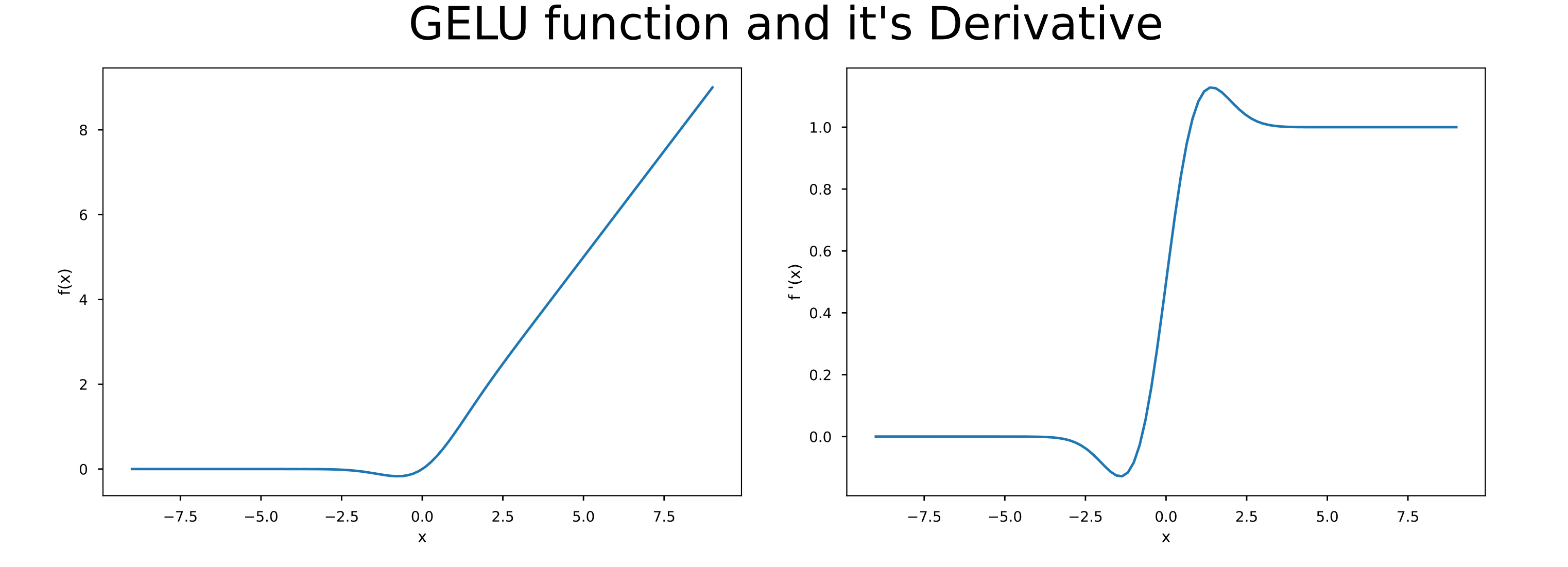
Indeed, this is relevant point, and we have inserted a discussion into the manuscript. From a technical point of view, our arguments require the underlying function to be smooth, which is why we make this assumption (we assume this is what the reviewer meant here – ReLU function is Lipschitz, but not smooth, and we require both). From a practical point of view, if one wants to use this with ReLU activation, a small modification that one can make is use a smooth approximation such as a GeLU instead (https://alaaalatif.github.io/gelu_imgs/gelu_viz-1.png), which is unlikely to make much of a difference to the result.

It is possible to have a result with ReLU activations, but then one needs to assume that the state is approximately random under the stationary distribution so that the update is “smooth on the average” (randomness means states are unlikely to fall near the point where the derivative of the ReLU changes, so that randomness acts as a smoother). This is what was done in the previous work Cai et al. (2019). Since we do not want to assume randomness of the state, we have to stick with smooth activations.
•

Moreover, in the left-hand side, the average cannot go inside the V since it is nonlinear. Then how can we derive a conclusion for $\theta_{t}$ ?

That is correct: the left hand side of the main theorem is not linear with respect to $\theta$ , so as the reviewer points out, we cannot put the average inside. However, it is enough to get that the error corresponding to a random iterate on $1,\ldots,T$ goes to zero – please see the second to last paragraph on page 6 of our paper. So this does lead to an algorithm: run projected TD for $T$ steps, then take a uniformly random iterate among those generated.

We acknowledge the reviewer’s point that this is a lot less nice than a bound on the last iterate $\theta_{T}$ . Unfortunately, this is a common issue in stochastic optimization going beyond RL – in many contexts it is possible to derive a bound on the error corresponding to a random iterate but quite challenging to derive a bound on the final iterate.

Given that we have clarified the main concern raised by the reviewer – namely, whether we are bounding an actual norm – we are wondering if the reviewer might be willing to re-evaluate their score of our paper. Regardless, we would like to thank the reviewer once again for their comments which led us to improve the paper in several significant ways.

3 Third Reviewer

•

Strength: the paper uses new techniques to analyze the convergence of neural TD. In particular, it utilize a combination of D-norm and Dirichlet norm to characterize the distance to the true value function. The reviewer believes that the analysis brings insight to the reinforcement learning community.

Thank you for the positive assessment of our work!

•

Weakness: The theoretical result seems a weak increment. It is not clear why changing the projection radius to constant can help the TD learning in practice. In fact, since the essential models considered are still linear models implied by the neural tangent kernel (NTK), the generalization error will be the same as the settings of previous neural TD works).

This is an interesting remark, and we thank the reviewer for bringing this is up – this gives us a chance to discuss the placement of this paper within NTK theory.

As a first response, though, note that our simulations show a strong improvement from choosing the projection radius to be a constant! Indeed, in Section 4, all the solid lines (constant projection radius) outperform the dashed lines ( $\sim m^{-1/2}$ projection radius) of the same color.

Now typical NTK analysis proceeds by arguing that, when the network is wide, it stays close to the initial condition during trainining, and is consequently approximately linear. The cleanest statement of this is in https://proceedings.neurips.cc/paper/2019/hash/ae614c557843b1df326cb29c57225459-Abstract.html, and previous papers on neural TD and neural Q-learning generally used that approach. But we do not see this in training. In fact, here is an additional set of graphs we generated that show the distance to the initial condition divided by the projection radius:

https://anonymous.4open.science/r/images_in_paper-87D6/dist.png

As can be seen, the iterates move to the boundary of the projection region in every case. In other words, the neural TD iterates move as far from the initial condition as they can.

A partial explanation for this is that the width ( $m=80$ to $m=160$ ) that we are simulating (with depths ranging from $3$ to $7$ ) is likely not large enough to be covered by the NTK-type results that ensure closeness to initial condition. As a further test of this, we plot the error measure

||\nabla V_{\theta_{t}}(s_{t})-\nabla V_{\theta_{0}}(s_{t})||,

which measures the linearity of the network during training: for a linear map, this measure is identically zero because the gradient would be constant. The results are at

https://anonymous.4open.science/r/images_in_paper-87D6/grad.png

Note that we show the graph starting at iteration/ $20=1$ , so that the graphs do not begin at zero. We see that the nonlinearity increases during training and is not close to zero, even for the networks with a small projection radius.

To summarize: choosing a constant projection radius strongly improves performance, results in approximations that are nonlinear and that move as far away as they can from their initial condition. These simulations (coupled with simulations that show improved performance already in the body of the paper) show the value of using a constant projection radius that does not decay with $m$ and also show why the model is not linear.

It is natural to wonder how this can be: indeed, the reviewers comments are supported by a large amount of NTK theory. We believe the answer is that the latest analyses of wide neural networks proceeded by showing that bounds on the nonlinearity decay with $m$ , allowing NTK-type proofs to be applicable to much lower values of the width $m$ , where the network is still sufficiently nonlinear to have low generalization error. The primary paper we rely on for this kind of analysis is https://proceedings.neurips.cc/paper/2020/hash/b7ae8fecf15b8b6c3c69eceae636d203-Abstract.html.

Indeed, one of the main novel things about this paper is that it is fundamentally nonlinear. We compare our result to the best nonlinear neural network and achieve a decaying error in the number of iterations $T$ and the width $m$ . We do this without any kind of representability assumption on the underlying policy. By contrast, previous papers on the subject made assumptions that explicitly forced the network to stay close to the initial condition. We argue that this is a conceptual improvement to the state-of-the-art and wonder if the reviewer might reconsider their characterization of this work as a “weak increment.”

•

From the computation cost perspective, it will be more interesting if the authors can show that the projection step can be totally discarded (just as most NTK works on supervised works do).

We have actually added this to the paper! Please see Section B of the supplementary information for an analysis of the unprojected case, though only for a single-hidden-layer. However, we want to push back a little here: we don’t want to do what most NTK works do, which is reduce the wide-case to something that stays close to initialization and is explicitly linear.

Our theorem says that if the distance between $\theta_{0}$ and $\theta^{*}$ is at most $C\delta\sqrt{m}$ , for some explicitly written out constant $C$ , then with probability $1-\delta$ , the iterates remain bounded, which we call event ${\cal A}$ . We then show that $E[||\theta_{t}-\theta^{*}||^{2}|{\cal A}]\rightarrow 0$ .

We do not believe it is possible to remove the projection entirely, not without assuming $m$ is so large that we stay in the “linear” regime. Indeed, our simulations for values of $m=80$ to $m=160$ with depths ranging from $3$ ro $7$ already show examples of divergence without projection.

4 Forth Reviewer

•

Given the wide usage of neural TD this paper provides a great contribution for the community The paper is well-written overall while being a theoretical paper.

Thank you for the positive assessment of our work! This paper is the culmination of over two years of work on our part trying to understand and clarify the literature of neural TD.
•

More tips around the applicability of the theorems to practitioners would have been great. For example ReLU, a widely used function, does not satisfy the assumption of the theorem.

Indeed, we acknowledge this is a shortcoming of our results, and we have included a discussion of this in the paper. From a technical point of view, our arguments require the underlying function to be smooth, which is why we make this assumption. From a practical point of view, if one wants to use this with ReLU activation, a small modification that one can make is use a smooth approximation such as a GeLU instead (https://alaaalatif.github.io/gelu_imgs/gelu_viz-1.png), which is unlikely to make much of a difference to the result.

It is possible to have a result with ReLU activations, but then one needs to assume that the state is approximately random under the stationary distribution so that the update is “smooth on the average” (randomness means states are unlikely to fall near the point where the derivative of the ReLU changes, so that randomness acts as a smoother). This is what was done in the previous work Cai et al. (2019). Since we do not want to assume randomness of the state, we have to stick with smooth activations.
•

I could not find the constant value of the omega for the results shown.

The constant $\omega$ can be anything! But then it appears in various bounds we obtain, so any choice of $\omega$ allows it to be incorporated into the $O(\cdot)$ notation. What is not allowed – in the sense that it would require modifying the arguments – is to choose $\omega=\sqrt{m}$ or some such.

Reference:

Xu, Pan, and Quanquan Gu. ”A finite-time analysis of Q-learning with neural network function approximation.” International Conference on Machine Learning. PMLR, 2020.

Liu, Chaoyue, Libin Zhu, and Misha Belkin. ”On the linearity of large non-linear models: when and why the tangent kernel is constant.” Advances in Neural Information Processing Systems 33 (2020): 15954-15964.

Cai, Qi, et al. ”Neural temporal-difference learning converges to global optima.” Advances in Neural Information Processing Systems 32 (2019).

Allen-Zhu, Zeyuan, Yuanzhi Li, and Zhao Song. ”A convergence theory for deep learning via over-parameterization.” International Conference on Machine Learning. PMLR, 2019.

Cayci, Semih, et al. ”Sample Complexity and Overparameterization Bounds for Temporal Difference Learning with Neural Network Approximation.” arXiv preprint arXiv:2103.01391 (2021).