

Spatial-Temporal-Decoupled Masked Pre-training for Spatiotemporal Forecasting
Abstract
Spatiotemporal forecasting techniques are significant for various domains such as transportation, energy, and weather. Accurate prediction of spatiotemporal series remains challenging due to the complex spatiotemporal heterogeneity. In particular, current end-to-end models are limited by input length and thus often fall into spatiotemporal mirage, i.e., similar input time series followed by dissimilar future values and vice versa. To address these problems, we propose a novel self-supervised pre-training framework Spatial-Temporal-Decoupled Masked Pre-training (STD-MAE) that employs two decoupled masked autoencoders to reconstruct spatiotemporal series along the spatial and temporal dimensions. Rich-context representations learned through such reconstruction could be seamlessly integrated by downstream predictors with arbitrary architectures to augment their performances. A series of quantitative and qualitative evaluations on six widely used benchmarks (PEMS03, PEMS04, PEMS07, PEMS08, METR-LA, and PEMS-BAY) are conducted to validate the state-of-the-art performance of STD-MAE. Codes are available at https://github.com/Jimmy-7664/STD-MAE.
1 Introduction
Spatiotemporal data collected by sensor networks has become a vital area of research with many real-world applications. It benefits from extra spatial context like sensor locations and road networks that reveal dependencies between sensors. Consequently, a key distinction from typical multivariate time series is that spatiotemporal data exhibits spatiotemporal heterogeneity. Specifically, while time series vary across different locations (urban centers against suburban areas) and day types (weekday versus weekend), they demonstrate consistent, predictable patterns within similar contexts. Hence, accurately predicting spatiotemporal data hinges on effectively capturing such heterogeneity.


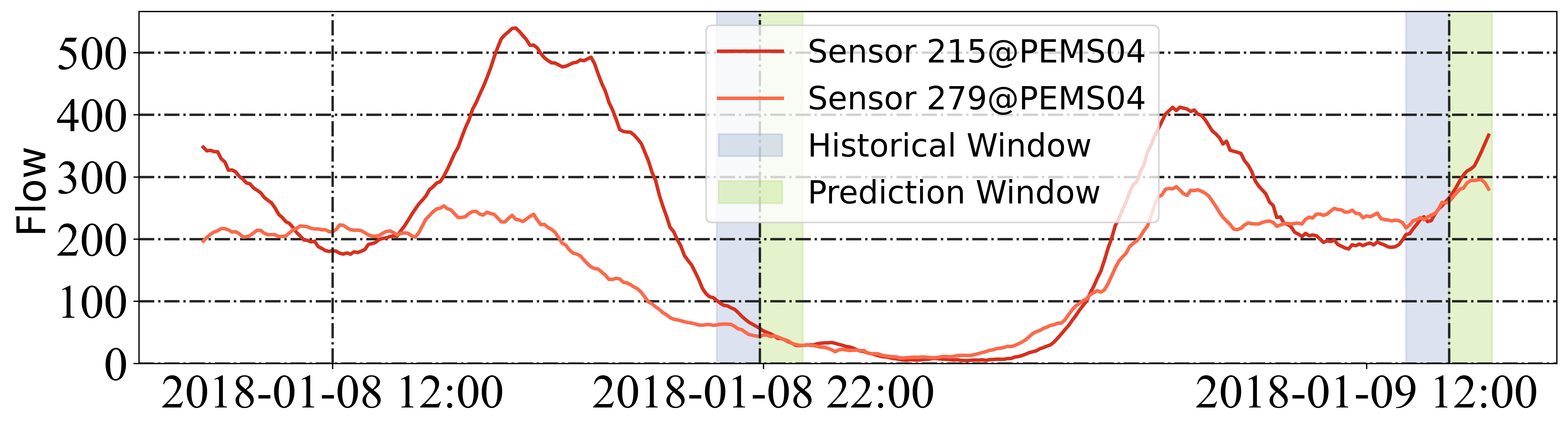
Figure 1(a) shows the traffic flow of sensor 7 in a spatiotemporal dataset PEMS04, revealing distinct weekday and weekend patterns especially during peak hours. Weekdays experience a morning rush hour peak, whereas weekend is more evenly distributed without significant peaks, illustrating temporal heterogeneity in weekly patterns. Additionally, Figure 1(b) displays the traffic flow of sensor 5, 86, 155, and 177 during the same period. Sensor 5 and 177 exhibit distinct peaks and troughs, while sensor 86 and 155 remain relatively stable throughout the day, demonstrating spatial heterogeneity. When the data scale is small, the heterogeneity is distinctly visible as shown above. However, when months of data from hundreds of sensors are given, the spatial and temporal heterogeneity becomes highly mixed. Previous researchers have done various attempts for spatiotemporal forecasting: embedding GCN into TCN Yu et al. (2018); Wu et al. (2019) or RNN Li et al. (2018); Bai et al. (2020), or applying transformer Jiang et al. (2023a); Liu et al. (2023) along spatiotemporal axes. But these models often have difficulty in distinguishing the spatial and temporal heterogeneity in a clear way. So learning clear heterogeneity is still the primary challenge for spatiotemporal forecasting.
Moreover, most of the existing models are trained in an end-to-end manner. Due to their high model complexity, their input horizons are often restricted to a short value (usually 12 steps) Yu et al. (2018); Wu et al. (2019); Song et al. (2020). This limitation will make the models suffer from an issue denoted as spatiotemporal mirage: i) dissimilar input time series followed by similar future values; ii) similar input time series followed by dissimilar future values. We illustrate this phenomenon by taking traffic flow of sensor 215 and 279 as an example in Figure 1(c). In the late evening, the two sensors show divergent historical data trends but similar future flow. Conversely, in the afternoon, their historical data trends align closely, yet their future data differ dramatically. Essentially, the reason behind this is that existing models can only capture the fragmented heterogeneity instead of the complete one. Therefore, how to make these models robust on such spatiotemporal mirage issue is the second challenge.
In this study, we focus our approach on learning clear and complete spatiotemporal heterogeneity through pre-training. In particular, masked pre-training has shown tremendous effectiveness in natural language processing Kenton and Toutanova (2019) and computer vision Bao et al. (2021). The core idea is to mask parts of the input sequence during pre-training, requiring the model to reconstruct the missing contents. In this way, the model learns context-rich representations which can augment various downstream tasks. Motivated by these benefits, we propose a novel spatial-temporal-decoupled masked pre-training framework called STD-MAE. It offers an effective and efficient solution for learning clear and complete spatiotemporal heterogeneity through pre-training. Such learned heterogeneity can be flawlessly integrated into downstream baselines to see through spatiotemporal mirages. In summary, our key contributions are as follows:
- •
We devise a pre-training framework on spatiotemporal data that can largely enhance downstream spatiotemporal predictors of arbitrary architectures without modifying their original structures.
- •
We propose a novel spatial-temporal-decoupled masking strategy to effectively learn spatial and temporal heterogeneity by capturing long-range context across spatial and temporal dimensions.
- •
We validate STD-MAE on six benchmarks (PEMS03, PEMS04, PEMS07, PEMS08, METR-LA, and PEMS-BAY) with typical backbones. Quantitative enhancement on baselines highlights the exceptional performance of STD-MAE. Qualitative analyses demonstrate its power to capture meaningful long-range spatiotemporal patterns.
2 Related Work
2.1 Spatiotemporal Forecasting
Spatiotemporal forecasting Jiang et al. (2021) aims to predict future spatiotemporal series by analyzing historical data. Early work mainly relied on traditional time series models Pan et al. (2012); Stock and Watson (2001). To capture the complex temporal dependencies, RNNs Hochreiter and Schmidhuber (1997); Chung et al. (2014) and CNNs Oord et al. (2016) have gained popularity for better modeling spatiotemporal data and achieving improved predictions.
Nevertheless, these models overlook crucial spatial correlations, limiting predictive performance on networked road systems. To further capture spatiotemporal features jointly, some studies integrate Graph Convolutional Networks (GCNs) with temporal models Yu et al. (2018); Li et al. (2018). Following this line of research, several novel spatiotemporal models have been proposed in recent years Wu et al. (2019); Xu et al. (2020); Bai et al. (2020); Cao et al. (2020); Wu et al. (2020); Guo et al. (2021a); Deng et al. (2022); Han et al. (2021); Jiang et al. (2023b); Deng et al. (2024). Attention mechanisms Vaswani et al. (2017) have also profoundly influenced spatiotemporal forecasting. A series of transformers Xu et al. (2020); Jiang et al. (2023a); Liu et al. (2023) are proposed and exhibit superior performance, highlighting their effectiveness in capturing the spatiotemporal relations. However, these end-to-end models only focus on short-term input that limits them to capture complete spatiotemporal dependencies.
2.2 Masked Pre-training
Masked pre-training has emerged as a highly effective technique for self-supervised representation learning in both natural language processing (NLP) and computer vision (CV). The key idea is to train models to predict masked-out parts of the input based on visible context. In NLP, approaches like BERT Kenton and Toutanova (2019) use masked language modeling to predict randomly masked tokens with bidirectional context. Subsequent models Liu et al. (2019); Lan et al. (2019) introduced more efficient masking techniques and demonstrated performance gains from longer pre-training. In CV, similar masking strategies have been adopted. Methods like BEiT Bao et al. (2021) and Masked AutoEncoder (MAE) He et al. (2022) mask out random patches of input images and do reconstruction based on unmasked patches. In both domains, masked pre-training produces substantial improvements on various downstream tasks.
Recently, many researchers have attempted to employ pre-training techniques on time series data to obtain superior hidden representations Nie et al. (2022); Shao et al. (2022b); Li et al. (2023). However, these methods are either channel-independent or neglect pre-training in the spatial dimension. Our proposed STD-MAE introduces a novel spatial-temporal-decoupled masking strategy during pre-training. By masking separately on spatial and temporal dimensions, the learned representations can effectively capture the intricate long-range heterogeneity in spatiotemporal data.
3 Problem Definition
Spatiotemporal forecasting is a specialized multivariate time series forecasting problem. Given multivariate time series in the past time steps, our goal is to predict the future time steps as: , where for the -th time step, is the number of spatial nodes, and is the number of the information channel. Here C=1 in our datasets.

4 Methodology
This section delves into the technical specifics of our proposed spatial-temporal-decoupled masked pre-training framework (STD-MAE) as delineated in Figure 2.
4.1 Spatial-Temporal Masked Pre-training
Spatial-Temporal-Decoupled Masking. In the standard spatiotemporal forecasting task, the input length for is usually equal to 12 (each step corresponds to 5-minute interval) Yu et al. (2018); Wu et al. (2019); Song et al. (2020), thus end-to-end models often fall into mirages outlined in Figure 1(c). So we intend to introduce a masked pre-training phase involving long-range input. Since spatiotemporal data has an additional temporal dimension compared to image data and an extra spatial dimension over language data, a straightforward idea is to apply the original masked pre-training Kenton and Toutanova (2019); He et al. (2022) directly by mixing the temporal and spatial dimension as one. However, this is unfeasible due to the square-level time and space complexity. Therefore, we propose a novel method called spatial-temporal-decoupled masking during masked pre-training. This approach separately executes mask-reconstruction tasks along temporal and spatial dimension. Such decoupled masking mechanism allows the model to learn representation that can capture clearer heterogeneity. With this wider and clearer view, downstream predictors can see through spatiotemporal mirages. Consequently, our method presents an efficient and effective solution for pre-training on spatiotemporal data, enhancing model robustness against the challenges posed by complex spatiotemporal heterogeneity and mirage.
Specifically, given an input spatiotemporal time series , we propose the following masking strategies: (1) Spatial Masking (S-Mask) randomly masks the time series of sensors, where is the masking ratio between 0 and 1. This results in a spatially masked input . (2) Temporal Masking (T-Mask) randomly masks the time series of time steps. This yields a temporally masked input . Both masking strategies can be viewed as random sampling from a Bernoulli distribution with expectation in the corresponding dimensions:
| (1) | ||||
Intuitively, S-Mask forces the model to reconstruct the data of masked sensors solely from the other visible sensors, thus capturing long-range spatial heterogeneity. Similarly, temporal heterogeneity can be learned by utilizing the intrinsic visible series to reconstruct the entire time series with T-Mask.
Spatial-Temporal-Decoupled Masked AutoEncoder. Building upon the spatial-temporal-decoupled masking technique, we further propose the spatial-temporal-decoupled masked autoencoder. It consists of a temporal autoencoder (T-MAE) and a spatial autoencoder (S-MAE), both having a similar architecture. S-MAE applies self-attention along spatial dimension, while T-MAE performs self-attention along temporal dimension. Specifically, we consider long input with length , typically spanning several days. However, directly utilizing such long sequences leads to computational and memory challenges. To address this, we apply a patch embedding technique Nie et al. (2022). The long input is divided into non-overlapping patches of length using a patch window . This yields a patched input . We then project through a fully connected layer to obtain the patch embedding , where is the embedding dimension. Moreover, to simultaneously encode spatial and temporal positional information, we implement a two-dimensional positional encoding Wang and Liu (2021). Given the patch embedding , the spatiotemporal positional encoding can be calculated as follows:
| (2) |
We choose sinusoidal positional encoding instead of learned positional encoding because it can handle inputs of arbitrary length. The patch embedding and positional encoding are summed to obtain the final input embedding .
This input embedding is subsequently masked by S-Mask and T-Mask strategies to obtain the visible spatial patch embedding and the visible temporal patch embedding . S-MAE and T-MAE generate spatial representations and temporal representations through a series of transformer layers, respectively. We denote as the number of masked sensors and as count of masked patches. By focusing only on visible parts, such design could reduce time and memory complexity.
A lightweight decoder is then applied to S-MAE and T-MAE to reconstruct the masked input. The spatial and temporal decoders each consists of a padding layer, a standard transformer layer, and a regression layer. Such asymmetrical design could dramatically reduce the pre-training time He et al. (2022). In the padding layer, we use a shared learnable mask token to indicate missing patches. Given spatial representation and temporal representation , spatial padding expands to spatial mask tokens while temporal padding expands to temporal mask tokens . The same spatiotemporal positional encoding as the encoders is added to and . Then we perform concatenation operations respectively as and to get the full set of patches . Subsequently, they are passed to the transformer layer. Finally, a regression layer is used to reconstruct the time series at the patch level. Formally, the reconstruction and for the spatially and temporally masked inputs can be derived by:
| (3) | |||
where is the spatial masked index and is the temporal masked index.
Following other masked pre-training architectures He et al. (2022); Tong et al. (2022), we compute the loss on the masked part only. Our loss function is computed by calculating the mean absolute error (MAE) between the ground truth and the reconstruction result. Given reconstruction and , the corresponding ground truth are and . The two loss functions in spatial and temporal can be calculated as:
| (4) | ||||
In summary, through the above spatial-temporal-decoupled masked pre-training, STD-MAE can capture clear and complete spatial and temporal heterogeneity.
4.2 Downstream Spatiotemporal Forecasting
STD-MAE can be seamlessly integrated into existing predictor structures. This operation is done by adding the spatial and temporal representations generated by STD-MAE to the hidden representation of the predictor. Concretely, we first feed long-range input with time steps into pre-trained spatial and temporal encoders to generate the corresponding spatial representation and temporal representation . Then, we apply a downstream spatiotemporal predictor with parameter to obtain the hidden representation of the widely-used short input through the following:
| (5) |
where is the hidden representation dimension of the predictor. To align with , we truncate the representation and of the last patches, and reshape these two representations to and . Next, we project these two representations into dimension through a two-layer MLP. Finally, the augmented representation could be derived by adding these representations together:
| (6) |
By far, includes representations generated by the predictor itself as well as the long-range spatial and temporal representations from STD-MAE, which can largely enhance the performance of the downstream spatiotemporal predictor.
Specifically, in our work, we choose GWNet Wu et al. (2019) as our predictor due to its superior performance. We obtain the final representation by aggregating the hidden states from the skip connections across the multiple spatiotemporal layers of GWNet, along with the corresponding spatial and temporal representations generated by the STD-MAE. The augmented representation is then fed into GWNet’s regression layers for prediction. Furthermore, we also test other classical spatiotemporal predictors with a variety of structures, i.e., DCRNN Li et al. (2018), MTGNN Wu et al. (2020), STID Shao et al. (2022a) and STAEformer Liu et al. (2023). These experiments demonstrate the generality of STD-MAE. Details could be found in our ablation study.
5 Experiment
5.1 Experimental Setup
Datasets. To thoroughly evaluate the proposed STD-MAE model, we conduct extensive experiments on six real-world spatiotemporal benchmark datasets as listed in Table 1: PEMS03, PEMS04, PEMS07, PEMS08 Song et al. (2020), METR-LA, and PEMS-BAY Li et al. (2018). The raw data has a fine-grained time resolution of 5 minutes between consecutive time steps. For data preprocessing, we perform Z-score normalization on the raw inputs.
| Datasets | #Sensors | #Time Steps | Time Interval |
|---|---|---|---|
| PEMS03 | 358 | 5min | 26208 |
| PEMS04 | 307 | 5min | 16992 |
| PEMS07 | 883 | 5min | 28224 |
| PEMS08 | 170 | 5min | 17856 |
| METR-LA | 207 | 5min | 34272 |
| PEMS-BAY | 325 | 5min | 52116 |
| Model | PEMS03 | PEMS04 | PEMS07 | PEMS08 | ||||||||
|---|---|---|---|---|---|---|---|---|---|---|---|---|
| MAE | RMSE | MAPE | MAE | RMSE | MAPE | MAE | RMSE | MAPE | MAE | RMSE | MAPE | |
| ARIMA Fang et al. (2021) | 35.31 | 47.59 | 33.78 | 33.73 | 48.80 | 24.18 | 38.17 | 59.27 | 19.46 | 31.09 | 44.32 | 22.73 |
| VAR Song et al. (2020) | 23.65 | 38.26 | 24.51 | 23.75 | 36.66 | 18.09 | 75.63 | 115.24 | 32.22 | 23.46 | 36.33 | 15.42 |
| SVR Song et al. (2020) | 21.97 | 35.29 | 21.51 | 28.70 | 44.56 | 19.20 | 32.49 | 50.22 | 14.26 | 23.25 | 36.16 | 14.64 |
| LSTM Song et al. (2020) | 21.33 | 35.11 | 23.33 | 27.14 | 41.59 | 18.20 | 29.98 | 45.84 | 13.20 | 22.20 | 34.06 | 14.20 |
| TCN Lan et al. (2022) | 19.31 | 33.24 | 19.86 | 31.11 | 37.25 | 15.48 | 32.68 | 42.23 | 14.22 | 22.69 | 35.79 | 14.04 |
| Transformer Vaswani et al. (2017) | 17.50 | 30.24 | 16.80 | 23.83 | 37.19 | 15.57 | 26.80 | 42.95 | 12.11 | 18.52 | 28.68 | 13.66 |
| DCRNN Li et al. (2018) | 18.18 | 30.31 | 18.91 | 24.70 | 38.12 | 17.12 | 25.30 | 38.58 | 11.66 | 17.86 | 27.83 | 11.45 |
| STGCN Yu et al. (2018) | 17.49 | 30.12 | 17.15 | 22.70 | 35.55 | 14.59 | 25.38 | 38.78 | 11.08 | 18.02 | 27.83 | 11.40 |
| ASTGCN Guo et al. (2019) | 17.69 | 29.66 | 19.40 | 22.93 | 35.22 | 16.56 | 28.05 | 42.57 | 13.92 | 18.61 | 28.16 | 13.08 |
| GWNet Wu et al. (2019) | 19.85 | 32.94 | 19.31 | 25.45 | 39.70 | 17.29 | 26.85 | 42.78 | 12.12 | 19.13 | 31.05 | 12.68 |
| STSGCN Song et al. (2020) | 17.48 | 29.21 | 16.78 | 21.19 | 33.65 | 13.90 | 24.26 | 39.03 | 10.21 | 17.13 | 26.80 | 10.96 |
| STFGNN Li and Zhu (2021) | 16.77 | 28.34 | 16.30 | 19.83 | 31.88 | 13.02 | 22.07 | 35.80 | 9.21 | 16.64 | 26.22 | 10.60 |
| STGODE Fang et al. (2021) | 16.50 | 27.84 | 16.69 | 20.84 | 32.82 | 13.77 | 22.99 | 37.54 | 10.14 | 16.81 | 25.97 | 10.62 |
| DSTAGNN Lan et al. (2022) | 15.57 | 27.21 | 14.68 | 19.30 | 31.46 | 12.70 | 21.42 | 34.51 | 9.01 | 15.67 | 24.77 | 9.94 |
| ST-WA Cirstea et al. (2022) | 15.17 | 26.63 | 15.83 | 19.06 | 31.02 | 12.52 | 20.74 | 34.05 | 8.77 | 15.41 | 24.62 | 9.94 |
| ASTGNN Guo et al. (2021b) | 15.07 | 26.88 | 15.80 | 19.26 | 31.16 | 12.65 | 22.23 | 35.95 | 9.25 | 15.98 | 25.67 | 9.97 |
| EnhanceNet Cirstea et al. (2021) | 16.05 | 28.33 | 15.83 | 20.44 | 32.37 | 13.58 | 21.87 | 35.57 | 9.13 | 16.33 | 25.46 | 10.39 |
| AGCRN Bai et al. (2020) | 16.06 | 28.49 | 15.85 | 19.83 | 32.26 | 12.97 | 21.29 | 35.12 | 8.97 | 15.95 | 25.22 | 10.09 |
| Z-GCNETs Chen et al. (2021) | 16.64 | 28.15 | 16.39 | 19.50 | 31.61 | 12.78 | 21.77 | 35.17 | 9.25 | 15.76 | 25.11 | 10.01 |
| STNorm Deng et al. (2021) | 15.32 | 25.93 | 14.37 | 19.21 | 32.30 | 13.05 | 20.59 | 34.86 | 8.61 | 15.39 | 24.80 | 9.91 |
| STEP Shao et al. (2022b) | 14.22 | 24.55 | 14.42 | 18.20 | 29.71 | 12.48 | 19.32 | 32.19 | 8.12 | 14.00 | 23.41 | 9.50 |
| PDFormer Jiang et al. (2023a) | 14.94 | 25.39 | 15.82 | 18.32 | 29.97 | 12.10 | 19.83 | 32.87 | 8.53 | 13.58 | 23.51 | 9.05 |
| STAEformer Liu et al. (2023) | 15.35 | 27.55 | 15.18 | 18.22 | 30.18 | 11.98 | 19.14 | 32.60 | 8.01 | 13.46 | 23.25 | 8.88 |
| STD-MAE (Ours) | 13.80 | 24.43 | 13.96 | 17.80 | 29.25 | 11.97 | 18.65 | 31.44 | 7.84 | 13.44 | 22.47 | 8.76 |
Baselines. We compare STD-MAE with the following baseline methods. ARIMA Fang et al. (2021), VAR Song et al. (2020), SVR Song et al. (2020), LSTM Song et al. (2020), TCN Lan et al. (2022), and Transformer Vaswani et al. (2017) are time series models. For spatiotemporal models, we select several typical methods including DCRNN Li et al. (2018), STGCN Yu et al. (2018), ASTGCN Guo et al. (2019), GWNet Wu et al. (2019), STSGCN Song et al. (2020), STFGNN Li and Zhu (2021), STGODE Fang et al. (2021), DSTAGNN Lan et al. (2022), ST-WA Cirstea et al. (2022), ASTGNN Guo et al. (2021b), EnhanceNet Cirstea et al. (2021), AGCRN Bai et al. (2020), Z-GCNETs Chen et al. (2021), STEP Shao et al. (2022b), PDFormer Jiang et al. (2023a) and STAEformer Liu et al. (2023).
Settings. Following previous work Song et al. (2020); Li and Zhu (2021); Fang et al. (2021); Jiang et al. (2023a); Guo et al. (2021b), we divide the PEMS03, PEMS04, PEMS07, and PEMS08 datasets into training, validation, and test sets according to a 6:2:2 ratio. For METR-LA and PEMS-BAY datasets, the training, validation, and test ratio is set to 7:1:2. During pre-training, the long input of the six datasets are set to 864, 864, 864, 2016, 864, and 864 time steps, respectively. For prediction, we set the length of both input and output to 12 steps. The embedding dimension is 96. The encoder has 4 transformer layers while the decoder has 1 transformer layer. The number of multi-attention heads in transformer layer is set to 4. We use a patch size of 12 to align with the forecasting input. is equal to 1, which means we truncate and keep the last one patch of and . The masking ratio is set to 0.25. Optimization is performed with Adam optimizer using an initial learning rate of 0.001 and mean absolute error (MAE) loss. For evaluation, we use MAE, root mean squared error (RMSE), and mean absolute percentage error (MAPE(%)). Performance in Table 2 is assessed by averaging over all 12 prediction steps. Experiments are mainly conducted on a Linux server with four NVIDIA GeForce RTX 3090 GPUs. To make fair and consistent comparison, they are all performed on BasicTS Shao et al. (2023) platform.
| GWNet | STEP | PDFormer | STD-MAE | |
|---|---|---|---|---|
| Horizon@3 MAE | 1.30 | 1.26 | 1.32 | 1.23 |
| Horizon@3 RMSE | 2.73 | 2.73 | 2.83 | 2.62 |
| Horizon@3 MAPE | 2.71 | 2.59 | 2.78 | 2.56 |
| Horizon@6 MAE | 1.63 | 1.55 | 1.64 | 1.53 |
| Horizon@6 RMSE | 3.73 | 3.58 | 3.79 | 3.53 |
| Horizon@6 MAPE | 3.73 | 3.43 | 3.71 | 3.42 |
| Horizon@12 MAE | 1.99 | 1.79 | 1.91 | 1.77 |
| Horizon@12 RMSE | 4.60 | 4.20 | 4.43 | 4.20 |
| Horizon@12 MAPE | 4.71 | 4.18 | 4.51 | 4.17 |
| GWNet | STEP | PDFormer | STD-MAE | |
|---|---|---|---|---|
| Horizon@3 MAE | 2.69 | 2.61 | 2.83 | 2.62 |
| Horizon@3 RMSE | 5.15 | 4.98 | 5.45 | 5.02 |
| Horizon@3 MAPE | 6.99 | 6.60 | 7.77 | 6.70 |
| Horizon@6 MAE | 3.08 | 2.96 | 3.20 | 2.99 |
| Horizon@6 RMSE | 6.20 | 5.97 | 6.46 | 6.07 |
| Horizon@6 MAPE | 8.47 | 7.96 | 9.19 | 8.04 |
| Horizon@12 MAE | 3.51 | 3.37 | 3.62 | 3.40 |
| Horizon@12 RMSE | 7.28 | 6.99 | 7.47 | 7.07 |
| Horizon@12 MAPE | 9.96 | 9.61 | 10.91 | 9.59 |
5.2 Overall Performance
The performance of models is listed in Table 2, Table 3, and Table 4. For a fair comparison, the reported results of the baseline models are taken from the original literature, which have been widely cited and validated in spatiotemporal forecasting. Across all datasets, our STD-MAE achieves superior performance over the baselines by a significant margin on all evaluation metrics. For other baselines, the spatiotemporal models clearly outperform the time series models due to their ability to capture spatiotemporal dependencies. In summary, the proposed STD-MAE framework significantly advances the state-of-the-art in spatiotemporal forecasting, demonstrating its ability to augment downstream predictors.
5.3 Ablation Study
Masking Ablation. We design four variants to validate the effectiveness of our spatial-temporal masking mechanism:
- •
S-MAE: Only masking on the spatial dimension.
- •
T-MAE: Only masking on the temporal dimension.
- •
STM-MAE: Using spatial-temporal-mixed masking.
- •
w/o Mask: Without applying any masked pre-training.

We report the experimental results on the PEMS03 and PEMS07 datasets. As illustrated in Figure 3, STD-MAE with spatial-temporal-decoupled masking significantly outperforms the ablated versions. T-MAE and S-MAE still improve over the original model although they can only partly capture the heterogeneity. For STM-MAE, we mix the spatial and temporal dimensions before randomly masking operation. The task of mixed masking is trivial which would lead to learn representation with less rich semantics. Overall, the results highlight the value of our proposed spatial-temporal-decoupled masked pre-training design for spatiotemporal forecasting.
Predictor Ablation. To evaluate the generality of STD-MAE, we test five downstream predictors with different backbones including GCN+RNN, GCN+TCN, Linear and Transformer:
- •
STD-MAE-DCRNN: Using DCRNN as the predictor.
- •
STD-MAE-MTGNN: Using MTGNN as the predictor.
- •
STD-MAE-STID: Using STID as the predictor.
- •
STD-MAE-STAE: Using STAEformer as the predictor.
- •
STD-MAE: Using GWNet as the predictor.
The experiments are conducted on the PEMS04 and PEMS08 datasets. Table 5 illustrates consistent and substantial performance gains across all five downstream spatiotemporal predictors when augmented with STD-MAE. This demonstrates the robustness of the representations generated by STD-MAE, which can benefit all kinds of downstream predictors regardless of architectures.
In conclusion, these ablation studies validate the effectiveness of STD-MAE’s decoupled design and the generality for enhancing downstream baselines.
| Model | PEMS04 | PEMS08 |
|---|---|---|
| MAE/RMSE/MAPE | MAE/RMSE/MAPE | |
| DCRNN | 19.63/31.24/13.52 | 15.21/24.11/10.04 |
| STD-MAE-DCRNN | 18.65/30.09/13.07 | 14.50/23.38/9.36 |
| MTGNN | 19.17/31.70/13.37 | 15.18/24.14/10.20 |
| STD-MAE-MTGNN | 18.72/31.03/12.72 | 14.84/23.58/9.58 |
| STID | 18.35/29.86/12.50 | 14.21/23.35/9.32 |
| STD-MAE-STID | 17.93/29.43/12.11 | 13.53/22.60/8.97 |
| STAEformer | 18.22/30.18/11.98 | 13.46/23.25/8.88 |
| STD-MAE-STAE | 17.92/29.37/12.11 | 13.30/22.51/8.82 |
| GWNet | 18.74/30.32/13.10 | 14.55/23.53/9.31 |
| STD-MAE (Ours) | 17.80/29.25/12.97 | 13.44/22.47/8.76 |
5.4 Hyper-parameter Study
Masking Ratio. We first conduct hyperparameter study by varying the masking ratio in , where the value is applied equally to S-MAE and T-MAE. As shown by Figure 4, a masking ratio of 0.25 yields the lowest error across all datasets, indicating optimal value. Prior work on masked language modeling with BERT Kenton and Toutanova (2019) utilizes a relatively low masking ratio of only 15% during pre-training. In contrast, masked autoencoders for image reconstruction He et al. (2022) and video modeling Tong et al. (2022) have found much higher optimal ratio of 75% and 90%, respectively. However, we find a somewhat lower optimal ratio of 25% for spatiotemporal time series modeling due to the fact that the long input time series required to provide extensive temporal context. This presents a challenge for reconstructing masked inputs, especially with spatial masking patterns that obstruct large contiguous blocks. Furthermore, our study demonstrates the importance of tuning masking specifically for spatiotemporal data. While an exact optimal is dataset-dependent, our results nonetheless show that relatively lower masking ratio is preferable for spatiotemporal time series.
Pre-training Length. We also study the effects of , which is the input length used in pre-training. Here we test different pre-training lengths of one day, three days, and a week on all four datasets. The results are shown in Table 6. In two out of the four datasets, a pre-training length of 3 days yields the best performance. Remarkably, compared to previous pre-training methodology, our approach demonstrates an enhanced capability to achieve superior performance with comparatively shorter pre-training lengths. These findings not only show the dynamic impact of pre-training length on the performance but also guide that the optimal pre-training length changes according to datasets.
| 288 | 864 | 2016 | |
|---|---|---|---|
| MAE / RMSE | MAE / RMSE | MAE / RMSE | |
| PEMS03 | 13.82/24.97 | 13.80/24.43 | 14.07/25.01 |
| PEMS04 | 17.94/29.26 | 17.80/29.26 | 17.84/29.27 |
| PEMS07 | 19.01/31.85 | 18.65/31.44 | 18.31/31.07 |
| PEMS08 | 13.74/22.71 | 13.66/22.68 | 13.44/22.47 |
5.5 Efficiency Test
Since STD-MAE introduce two decoupled autoencoders to encode spatial and temporal representation, efficiency might be a concern. However, due to the decoupled design of STD-MAE, it still outperforms in efficiency compare to other pretrained model especially for datasets with a large amount of sensors. Specifically, compared to non-decoupled pre-training methods, our decoupled time complexity is . We report the total training time for pre-training and forecasting per sample of four datasets as Table 7.
| # Sensors | STEP | STD-MAE | Improvement | |
|---|---|---|---|---|
| PEMS03 | 358 | 108ms | 50ms | 53.7% |
| PEMS04 | 307 | 73ms | 34ms | 53.9% |
| PEMS07 | 883 | 516ms | 142ms | 72.5% |
| PEMS08 | 170 | 62ms | 48ms | 22.6% |
5.6 Case Study
Reconstruction Accuracy in Pre-training. STD-MAE exhibits a robust capacity for reconstructing long time series by relying solely on the partially observed sensor recordings, as shown in Figures 5(a) and 5(b). The shaded area indicates the masked region. Temporal reconstruction closely matches the ground truth in terms of periodicity and trends. This suggests STD-MAE successfully acquires generalized knowledge of temporal patterns. Similarly, STD-MAE could restore entirely masked sensors based on contextual data from spatially related sensors, indicating it also gains meaningful spatial correlations. Overall, STD-MAE appears to learn rich spatiotemporal representations through pre-training.


Robustness on Spatiotemporal Mirage. In Figure 6, we present a comparative analysis of the prediction results from GWNet and STD-MAE for two spatiotemporal mirages in Figure 1(c). The input and prediction windows are denoted by purple and green backgrounds, respectively. A pivotal finding is that GWNet exhibits a limitation in distinguishing spatiotemporal mirages in Figures 6(a) and 6(c). In contrast, STD-MAE performs a significant accuracy in these situations as shown in Figures 6(b) and 6(d). The pre-trained component in STD-MAE remarkably enhances GWNet’s ability to distinguish spatiotemporal mirages arising from heterogeneity.
6 Conclusion
In this study, we propose STD-MAE, a novel spatial-temporal-decoupled masked pre-training framework for spatiotemporal forecasting. In the pre-training phase, a novel spatial-temporal-decoupled masking approach is utilized to effectively model the heterogeneity of spatiotemporal data. For forecasting phase, the hidden representations generated by STD-MAE are leveraged to boost the performance of downstream spatiotemporal predictors. Comprehensive experiments and in-depth analyses conducted on six benchmark datasets demonstrate the superiority of STD-MAE.
Acknowledgment
This work was supported by JST CREST Grant Number JPMJCR21M2 including AIP challenge program and JSPS KAKENHI Grant Number JP24K02996.
References
- Bai et al. [2020] Lei Bai, Lina Yao, Can Li, Xianzhi Wang, and Can Wang. Adaptive graph convolutional recurrent network for traffic forecasting. Advances in Neural Information Processing Systems, 33:17804–17815, 2020.
- Bao et al. [2021] Hangbo Bao, Li Dong, Songhao Piao, and Furu Wei. Beit: Bert pre-training of image transformers. In International Conference on Learning Representations, 2021.
- Cao et al. [2020] Defu Cao, Yujing Wang, Juanyong Duan, Ce Zhang, Xia Zhu, Congrui Huang, Yunhai Tong, Bixiong Xu, Jing Bai, Jie Tong, et al. Spectral temporal graph neural network for multivariate time-series forecasting. Advances in Neural Information Processing Systems, 33:17766–17778, 2020.
- Chen et al. [2021] Yuzhou Chen, Ignacio Segovia, and Yulia R Gel. Z-gcnets: Time zigzags at graph convolutional networks for time series forecasting. In International Conference on Machine Learning, pages 1684–1694. PMLR, 2021.
- Chung et al. [2014] Junyoung Chung, Caglar Gulcehre, KyungHyun Cho, and Yoshua Bengio. Empirical evaluation of gated recurrent neural networks on sequence modeling. arXiv preprint arXiv:1412.3555, 2014.
- Cirstea et al. [2021] Razvan-Gabriel Cirstea, Tung Kieu, Chenjuan Guo, Bin Yang, and Sinno Jialin Pan. Enhancenet: Plugin neural networks for enhancing correlated time series forecasting. In 2021 IEEE 37th International Conference on Data Engineering (ICDE), pages 1739–1750. IEEE, 2021.
- Cirstea et al. [2022] Razvan-Gabriel Cirstea, Bin Yang, Chenjuan Guo, Tung Kieu, and Shirui Pan. Towards spatio-temporal aware traffic time series forecasting. In 2022 IEEE 38th International Conference on Data Engineering (ICDE), pages 2900–2913. IEEE, 2022.
- Deng et al. [2021] Jinliang Deng, Xiusi Chen, Renhe Jiang, Xuan Song, and Ivor W Tsang. St-norm: Spatial and temporal normalization for multi-variate time series forecasting. In Proceedings of the 27th ACM SIGKDD Conference on Knowledge Discovery & Data Mining, pages 269–278, 2021.
- Deng et al. [2022] Jinliang Deng, Xiusi Chen, Renhe Jiang, Xuan Song, and Ivor W Tsang. A multi-view multi-task learning framework for multi-variate time series forecasting. IEEE Transactions on Knowledge and Data Engineering, 2022.
- Deng et al. [2024] Jinliang Deng, Xiusi Chen, Renhe Jiang, Du Yin, Yi Yang, Xuan Song, and Ivor W Tsang. Disentangling structured components: Towards adaptive, interpretable and scalable time series forecasting. IEEE Transactions on Knowledge and Data Engineering, 2024.
- Fang et al. [2021] Zheng Fang, Qingqing Long, Guojie Song, and Kunqing Xie. Spatial-temporal graph ode networks for traffic flow forecasting. In Proceedings of the 27th ACM SIGKDD Conference on Knowledge Discovery & Data Mining, pages 364–373, 2021.
- Guo et al. [2019] Shengnan Guo, Youfang Lin, Ning Feng, Chao Song, and Huaiyu Wan. Attention based spatial-temporal graph convolutional networks for traffic flow forecasting. In Proceedings of the AAAI conference on artificial intelligence, volume 33, pages 922–929, 2019.
- Guo et al. [2021a] Kan Guo, Yongli Hu, Yanfeng Sun, Sean Qian, Junbin Gao, and Baocai Yin. Hierarchical graph convolution networks for traffic forecasting. In Proceedings of the AAAI Conference on Artificial Intelligence, volume 35, pages 151–159, 2021.
- Guo et al. [2021b] Shengnan Guo, Youfang Lin, Huaiyu Wan, Xiucheng Li, and Gao Cong. Learning dynamics and heterogeneity of spatial-temporal graph data for traffic forecasting. IEEE Transactions on Knowledge and Data Engineering, 2021.
- Han et al. [2021] Liangzhe Han, Bowen Du, Leilei Sun, Yanjie Fu, Yisheng Lv, and Hui Xiong. Dynamic and multi-faceted spatio-temporal deep learning for traffic speed forecasting. In Proceedings of the 27th ACM SIGKDD Conference on Knowledge Discovery & Data Mining, pages 547–555, 2021.
- He et al. [2022] Kaiming He, Xinlei Chen, Saining Xie, Yanghao Li, Piotr Dollár, and Ross Girshick. Masked autoencoders are scalable vision learners. In Proceedings of the IEEE/CVF conference on computer vision and pattern recognition, pages 16000–16009, 2022.
- Hochreiter and Schmidhuber [1997] Sepp Hochreiter and Jürgen Schmidhuber. Long short-term memory. Neural computation, 9(8):1735–1780, 1997.
- Jiang et al. [2021] Renhe Jiang, Du Yin, Zhaonan Wang, Yizhuo Wang, Jiewen Deng, Hangchen Liu, Zekun Cai, Jinliang Deng, Xuan Song, and Ryosuke Shibasaki. Dl-traff: Survey and benchmark of deep learning models for urban traffic prediction. In Proceedings of the 30th ACM International Conference on Information & Knowledge Management, pages 4515–4525, 2021.
- Jiang et al. [2023a] Jiawei Jiang, Chengkai Han, Wayne Xin Zhao, and Jingyuan Wang. Pdformer: Propagation delay-aware dynamic long-range transformer for traffic flow prediction. In AAAI. AAAI Press, 2023.
- Jiang et al. [2023b] Renhe Jiang, Zhaonan Wang, Jiawei Yong, Puneet Jeph, Quanjun Chen, Yasumasa Kobayashi, Xuan Song, Shintaro Fukushima, and Toyotaro Suzumura. Spatio-temporal meta-graph learning for traffic forecasting. In Proceedings of the AAAI Conference on Artificial Intelligence, volume 37, pages 8078–8086, 2023.
- Kenton and Toutanova [2019] Jacob Devlin Ming-Wei Chang Kenton and Lee Kristina Toutanova. Bert: Pre-training of deep bidirectional transformers for language understanding. In Proceedings of NAACL-HLT, pages 4171–4186, 2019.
- Lan et al. [2019] Zhenzhong Lan, Mingda Chen, Sebastian Goodman, Kevin Gimpel, Piyush Sharma, and Radu Soricut. Albert: A lite bert for self-supervised learning of language representations. arXiv preprint arXiv:1909.11942, 2019.
- Lan et al. [2022] Shiyong Lan, Yitong Ma, Weikang Huang, Wenwu Wang, Hongyu Yang, and Pyang Li. Dstagnn: Dynamic spatial-temporal aware graph neural network for traffic flow forecasting. In International conference on machine learning, pages 11906–11917. PMLR, 2022.
- Li and Zhu [2021] Mengzhang Li and Zhanxing Zhu. Spatial-temporal fusion graph neural networks for traffic flow forecasting. In Proceedings of the AAAI Conference on Artificial Intelligence, volume 35, pages 4189–4196, 2021.
- Li et al. [2018] Yaguang Li, Rose Yu, Cyrus Shahabi, and Yan Liu. Diffusion convolutional recurrent neural network: Data-driven traffic forecasting. In International Conference on Learning Representations, 2018.
- Li et al. [2023] Zhe Li, Zhongwen Rao, Lujia Pan, Pengyun Wang, and Zenglin Xu. Ti-mae: Self-supervised masked time series autoencoders. arXiv preprint arXiv:2301.08871, 2023.
- Liu et al. [2019] Yinhan Liu, Myle Ott, Naman Goyal, Jingfei Du, Mandar Joshi, Danqi Chen, Omer Levy, Mike Lewis, Luke Zettlemoyer, and Veselin Stoyanov. Roberta: A robustly optimized bert pretraining approach. arXiv preprint arXiv:1907.11692, 2019.
- Liu et al. [2023] Hangchen Liu, Zheng Dong, Renhe Jiang, Jiewen Deng, Jinliang Deng, Quanjun Chen, and Xuan Song. Spatio-temporal adaptive embedding makes vanilla transformer sota for traffic forecasting. In Proceedings of the 32nd ACM International Conference on Information and Knowledge Management, pages 4125–4129, 2023.
- Nie et al. [2022] Yuqi Nie, Nam H Nguyen, Phanwadee Sinthong, and Jayant Kalagnanam. A time series is worth 64 words: Long-term forecasting with transformers. In The Eleventh International Conference on Learning Representations, 2022.
- Oord et al. [2016] Aaron van den Oord, Sander Dieleman, Heiga Zen, Karen Simonyan, Oriol Vinyals, Alex Graves, Nal Kalchbrenner, Andrew Senior, and Koray Kavukcuoglu. Wavenet: A generative model for raw audio. arXiv preprint arXiv:1609.03499, 2016.
- Pan et al. [2012] Bei Pan, Ugur Demiryurek, and Cyrus Shahabi. Utilizing real-world transportation data for accurate traffic prediction. In 2012 ieee 12th international conference on data mining, pages 595–604. IEEE, 2012.
- Shao et al. [2022a] Zezhi Shao, Zhao Zhang, Fei Wang, Wei Wei, and Yongjun Xu. Spatial-temporal identity: A simple yet effective baseline for multivariate time series forecasting. In Proceedings of the 31st ACM International Conference on Information & Knowledge Management, pages 4454–4458, 2022.
- Shao et al. [2022b] Zezhi Shao, Zhao Zhang, Fei Wang, and Yongjun Xu. Pre-training enhanced spatial-temporal graph neural network for multivariate time series forecasting. In Proceedings of the 28th ACM SIGKDD Conference on Knowledge Discovery and Data Mining, pages 1567–1577, 2022.
- Shao et al. [2023] Zezhi Shao, Fei Wang, Yongjun Xu, Wei Wei, Chengqing Yu, Zhao Zhang, Di Yao, Guangyin Jin, Xin Cao, Gao Cong, et al. Exploring progress in multivariate time series forecasting: Comprehensive benchmarking and heterogeneity analysis. arXiv preprint arXiv:2310.06119, 2023.
- Song et al. [2020] Chao Song, Youfang Lin, Shengnan Guo, and Huaiyu Wan. Spatial-temporal synchronous graph convolutional networks: A new framework for spatial-temporal network data forecasting. In Proceedings of the AAAI Conference on Artificial Intelligence, volume 34, pages 914–921, 2020.
- Stock and Watson [2001] James H Stock and Mark W Watson. Vector autoregressions. Journal of Economic perspectives, 15(4):101–115, 2001.
- Tong et al. [2022] Zhan Tong, Yibing Song, Jue Wang, and Limin Wang. Videomae: Masked autoencoders are data-efficient learners for self-supervised video pre-training. Advances in neural information processing systems, 35:10078–10093, 2022.
- Vaswani et al. [2017] Ashish Vaswani, Noam Shazeer, Niki Parmar, Jakob Uszkoreit, Llion Jones, Aidan N Gomez, Łukasz Kaiser, and Illia Polosukhin. Attention is all you need. Advances in neural information processing systems, 30, 2017.
- Wang and Liu [2021] Zelun Wang and Jyh-Charn Liu. Translating math formula images to latex sequences using deep neural networks with sequence-level training. International Journal on Document Analysis and Recognition (IJDAR), 24(1-2):63–75, 2021.
- Wu et al. [2019] Zonghan Wu, Shirui Pan, Guodong Long, Jing Jiang, and Chengqi Zhang. Graph wavenet for deep spatial-temporal graph modeling. In IJCAI, 2019.
- Wu et al. [2020] Zonghan Wu, Shirui Pan, Guodong Long, Jing Jiang, Xiaojun Chang, and Chengqi Zhang. Connecting the dots: Multivariate time series forecasting with graph neural networks. In Proceedings of the 26th ACM SIGKDD International Conference on Knowledge Discovery & Data Mining, pages 753–763, 2020.
- Xu et al. [2020] Mingxing Xu, Wenrui Dai, Chunmiao Liu, Xing Gao, Weiyao Lin, Guo-Jun Qi, and Hongkai Xiong. Spatial-temporal transformer networks for traffic flow forecasting. arXiv preprint arXiv:2001.02908, 2020.
- Yu et al. [2018] Bing Yu, Haoteng Yin, and Zhanxing Zhu. Spatio-temporal graph convolutional networks: a deep learning framework for traffic forecasting. In Proceedings of the 27th International Joint Conference on Artificial Intelligence, pages 3634–3640, 2018.