The ${\rm SL}(2,\mathbb{C})$-character variety of an arborescent knot

Abstract

We describe a procedure for computing the ${\rm SL}(2,\mathbb{C})$-character variety of an arborescent knot. Along the way, we clarify several facts about representations of arborescent tangles. Then we study a family of hyperbolic knots whose exteriors contain closed essential surfaces, showing that each of these knots has $1$-dimensional character variety. This provides infinitely many positive answers to a question of Boyer and Zhang posed in 1998.

Keywords: arborescent knot; ${\rm SL}(2,\mathbb{C})$-character variety; irreducible representation; rational tangle
MSC2020: 57K10, 57K31

1 Introduction

Fix $G={\rm SL}(2,\mathbb{C})$ throughout. Given a finitely presented group $\Gamma$, a homomorphism $\rho:\Gamma\to G$ is called a $G$-representation of $\Gamma$. Call $\rho$ reducible if the elements of ${\rm Im}(\rho)$ have a common eigenvector, and irreducible otherwise. Call $\mathcal{R}(\Gamma):=\hom(\Gamma,G)$ the $G$-representation variety of $\Gamma$. For each $\rho\in\mathcal{R}(\Gamma)$, its character is defined as the function $\chi_{\rho}:\Gamma\to\mathbb{C}$ sending $x$ to ${\rm tr}(\rho(x))$. It is known that two irreducible representations $\rho,\rho^{\prime}$ have the same character if and only if they are conjugate, meaning that there exists $\mathbf{a}\in G$ such that $\rho^{\prime}(x)=\mathbf{a}\rho(x)\mathbf{a}^{-1}$ for all $x\in\Gamma$. The set $\mathcal{X}(\Gamma)=\{\chi_{\rho}\colon\rho\in\mathcal{R}(\Gamma)\}$ turns out to be an algebraic set, and is called the $G$-character variety of $\Gamma$. The subset $\mathcal{X}^{\rm irr}(\Gamma)$ of $\mathcal{X}(\Gamma)$ consisting of characters of irreducible representations is Zariski open, and is called the irreducible character variety.

For a $3$-manifold $M$, abbreviate $\mathcal{X}(\pi_{1}(M))$ to $\mathcal{X}(M)$. For a link $L\subset S^{3}$, let $\pi(L)=\pi_{1}(E_{L})$, where $E_{L}$ denotes the exterior of $L$, abbreviate $\mathcal{R}(\pi(L))$ to $\mathcal{R}(L)$ and call it the $G$-representation variety of $L$, and so forth.

Nowadays, character varieties play a significant role in low-dimensional topology, but are still considered notoriously difficult to compute. Very little is known about character varieties of general links. So it is worthwhile to describe $\mathcal{X}(L)$ for as many links $L$ as possible. On the other hand, we believe it hopeful to reveal structural properties for certain families of knots.

In [4] the author proposed a method for determining $\mathcal{X}^{\rm irr}(K)$ for each Montesinos knot $K$, and showed a decomposition $\mathcal{X}^{\rm irr}(K)=\mathcal{X}_{0}\sqcup\mathcal{X}_{1}\sqcup\mathcal{X}_{2}\sqcup\mathcal{X}^{\prime}$, such that each part has a distinguished feature. In this paper, we aim to extend the scope to arborescent knots. These knots form an interesting class, and had been studied extensively by Bonahon and Siebenmann [1], and are abundant among those with small number of crossings. In particular, among the $84$ knots with at most $9$ crossings in Rolfsen’s table, only $8_{18},9_{34},9_{39},9_{40},9_{41},9_{47},9_{49}$ are non-arborescent. As another important fact, almost all arborescent knots are hyperbolic [17].

It can be expected that new phenomena will be uncovered by studying knots other than “small” knots such as torus knots, 2-bridge knots and 3-strand pretzel knots, as usually treated in the literature.

Here by studying a family of arborescent knots, we positively answer the following question of Boyer and Zhang, posed as [2, Question 10.3].

Question 1.1.

Is there a hyperbolic knot whose exterior contains a closed essential surface but the ${\rm PSL}(2,\mathbb{C})$-character variety is 1-dimensional?

This is the first time to find infinitely many hyperbolic knots whose exteriors contain essential surfaces not detected by ideal points of character varieties. See Section 4.6 for detailed discussions.

The content is organized as follows. In Section 2, we present some preliminaries on $2\times 2$ matrices and tangles, as well as representations of tangles. In Section 3, we describe a procedure of computing $\mathcal{X}^{\rm irr}(K)$ for arborescent knots $K$. Most of the work is concerned with representations of arborescent tangles, about which several important facts are clarified. In Section 4, we study a family of hyperbolic arborescent knots, showing that $\dim\mathcal{X}(K)=1$ for each $K$ in that family. It is known that $E_{K}$ contains closed essential surfaces, thus $K$ fulfills the required conditions in Question 1.1.

2 Preparations

2.1 Algebraic aspects

We always use bold letters to denote elements of $G$.

Let $\mathsf{T}_{+},\mathsf{T}_{-},\mathsf{T}_{0}$ respectively denote the subset of $G$ consisting of upper-triangular, lower-triangular, diagonal matrices.

Let $\mathbf{e}$ denote the $2\times 2$ identity matrix. Let

$$\mathbf{p} =\left(\begin{array}[]{cc}1&1\\ 0&1\end{array}\right),\qquad \mathbf{d}(\kappa) =\left(\begin{array}[]{cc}\kappa&0\\ 0&\kappa^{-1}\end{array}\right),$$

$$\mathbf{u}_{\kappa}(\xi) =\left(\begin{array}[]{cc}\kappa&\xi\\ 0&\kappa^{-1}\end{array}\right),\qquad \mathbf{l}_{\kappa}(\xi) =\left(\begin{array}[]{cc}\kappa&0\\ \xi&\kappa^{-1}\end{array}\right).$$

For $t\in\mathbb{C}$, let $G(t)=\{\mathbf{x}\in G\setminus\{\pm\mathbf{e}\}\colon{\rm tr}(\mathbf{x})=t\}$.

For $\mathbf{a},\mathbf{b}\in G$, let $\mathbf{a}\lrcorner\mathbf{b}=\mathbf{a}\mathbf{b}\mathbf{a}^{-1}$.

Call a tuple $(\mathbf{a}_{1},\ldots,\mathbf{a}_{k})\in G^{k}$ reducible if $\mathbf{a}_{1},\ldots,\mathbf{a}_{k}$ share an eigenvector, and irreducible otherwise. Say that $(\mathbf{a}^{\prime}_{1},\ldots,\mathbf{a}^{\prime}_{k})$ is conjugate to $(\mathbf{a}_{1},\ldots,\mathbf{a}_{k})$ if there exists $\mathbf{c}\in G$ with $\mathbf{c}\lrcorner\mathbf{a}_{i}=\mathbf{a}^{\prime}_{i}$ for $1\leq i\leq k$. Call a reducible pair $(\mathbf{a}_{1},\mathbf{a}_{2})$ nonabelian reducible (NR for short) if $\mathbf{a}_{1}\mathbf{a}_{2}\neq\mathbf{a}_{2}\mathbf{a}_{1}$.

For $\lambda\neq-1$ and $\mu\neq 0$, put

$$\mathbf{h}_{t}^{\lambda}(\mu)=\frac{1}{\lambda+1}\left(\begin{array}[]{cc}\lambda t&\mu\\ (t^{2}-\lambda-\lambda^{-1}-2)\lambda\mu^{-1}&t\end{array}\right).$$

For $t\neq 0$, put

$$\mathbf{k}_{t}(\alpha)=\left(\begin{array}[]{cc}\alpha+t/2&(t^{2}/4-1-\alpha^{2})/(2t)\\ 2t&-\alpha+t/2\end{array}\right).$$

By direct computation,

$${\rm tr}\big(\mathbf{h}_{t}^{\lambda}(\mu)^{-1}\mathbf{h}_{t}^{\lambda}(\nu)\big)=\frac{2t^{2}+(\lambda+\lambda^{-1}+2-t^{2})(\mu\nu^{-1}+\mu^{-1}\nu)}{\lambda+\lambda^{-1}+2}.$$ (1)

For the following lemma, refer to [4, Lemma 2.2]:

Lemma 2.1.

Let $\mathbf{a}_{1},\mathbf{a}_{2}\in G(t)$.

1. If $\mathbf{a}_{1}\mathbf{a}_{2}=\mathbf{d}(\lambda)$ with $\lambda+\lambda^{-1}\neq\pm 2,t^{2}-2$, then $\mathbf{a}_{1}=\mathbf{h}_{t}^{\lambda}(-\lambda\mu)$, $\mathbf{a}_{2}=\mathbf{h}_{t}^{\lambda}(\mu)$ for some $\mu\neq 0$.

2. If $\mathbf{a}_{1}\mathbf{a}_{2}=\mathbf{p}$, then $\mathbf{a}_{1},\mathbf{a}_{2}\in\mathsf{T}_{+}$; more precisely, $\mathbf{a}_{1}=\mathbf{u}_{\kappa^{-1}}(\xi)$, $\mathbf{a}_{2}=\mathbf{u}_{\kappa}(\kappa-\xi)$ for some $\xi$ and $\kappa$ with $\kappa+\kappa^{-1}=t$.

3. If $\mathbf{a}_{1}\mathbf{a}_{2}=-\mathbf{p}$ and $t\neq 0$, then $\mathbf{a}_{1}=\mathbf{k}_{t}(\alpha+t)$, $\mathbf{a}_{2}=\mathbf{k}_{t}(\alpha)$ for some $\alpha$.

4. If $\mathbf{a}_{1}\mathbf{a}_{2}=\mathbf{d}(\kappa^{2})$ with $\kappa+\kappa^{-1}=t\neq 0,\pm 2$, then one of the following cases occurs: (i) $\mathbf{a}_{1}=\mathbf{a}_{2}=\mathbf{d}(\kappa)$; (ii) $\mathbf{a}_{1}=\mathbf{u}_{\kappa}(\kappa^{2}\xi)$, $\mathbf{a}_{2}=\mathbf{u}_{\kappa}(-\xi)$ for some $\xi\neq 0$; (iii) $\mathbf{a}_{1}=\mathbf{l}_{\kappa}(-\xi)$, $\mathbf{a}_{2}=\mathbf{l}_{\kappa}(\kappa^{2}\xi)$ for some $\xi\neq 0$.

5. The pair $(\mathbf{a}_{1},\mathbf{a}_{2})$ is reducible if and only if ${\rm tr}(\mathbf{a}_{1}\mathbf{a}_{2})\in\{2,t^{2}-2\}$.

In the case $\mathbf{a}_{1}\mathbf{a}_{2}=\mathbf{p}$, the original statement in [4] is refined here.

Whenever ${\rm tr}(\mathbf{a}_{1}\mathbf{a}_{2})=\lambda+\lambda^{-1}\neq\pm 2,t^{2}-2$, up to conjugacy we may assume $\mathbf{a}_{1}\mathbf{a}_{2}=\mathbf{d}(\lambda)$, so that $\mathbf{a}_{1}=\mathbf{h}_{t}^{\lambda}(-\lambda\mu)$ and $\mathbf{a}_{2}=\mathbf{h}_{t}^{\lambda}(\mu)$ for some $\mu\neq 0$. This will often simplify computations.

To illustrate the convenience, we establish a useful lemma:

Lemma 2.2.

Suppose $\mathbf{a}_{1},\mathbf{a}_{2},\mathbf{a}_{3},\mathbf{a}_{4}\in G(t)$ satisfy $\mathbf{a}_{1}\mathbf{a}_{2}=\mathbf{a}_{3}\mathbf{a}_{4}=\mathbf{c}$, with ${\rm tr}(\mathbf{c})\neq 2,t^{2}-2$.

1. If ${\rm tr}(\mathbf{a}_{1}\mathbf{a}_{3}^{-1})=2$, then $\mathbf{a}_{1}=\mathbf{a}_{3}$ and $\mathbf{a}_{2}=\mathbf{a}_{4}$.

2. If $t\neq 0$, then $\mathbf{c}\neq-\mathbf{e}$, $\mathbf{a}_{1}\neq\mathbf{a}_{3}^{-1}$ and $\mathbf{a}_{2}\neq\mathbf{a}_{4}^{-1}$.

Proof.

(i) Suppose ${\rm tr}(\mathbf{a}_{1}\mathbf{a}_{3}^{-1})=2$. Assume $\mathbf{a}_{3}^{-1}\mathbf{a}_{1}\neq\mathbf{e}$. Then up to conjugacy we may assume $\mathbf{a}_{3}^{-1}\mathbf{a}_{1}=\mathbf{p}$, so that also $\mathbf{a}_{4}\mathbf{a}_{2}^{-1}=\mathbf{p}$. By Lemma 2.1 (b), $\mathbf{a}_{3},\mathbf{a}_{1}\in\mathsf{T}_{+}$, and $\mathbf{a}_{4},\mathbf{a}_{2}\in\mathsf{T}_{+}$. This would imply ${\rm tr}(\mathbf{c})\in\{2,t^{2}-2\}$, contradicting the assumption. Thus, $\mathbf{a}_{1}=\mathbf{a}_{3}$, and $\mathbf{a}_{2}=\mathbf{a}_{4}$.

(ii) When ${\rm tr}(\mathbf{c})\neq-2$, up to conjugacy we may assume $\mathbf{c}=\mathbf{d}(\lambda)$ with $\lambda+\lambda^{-1}\neq\pm 2,t^{2}-2$. By Lemma 2.1 (a), $\mathbf{a}_{2}=\mathbf{h}^{\lambda}_{t}(\mu)$, $\mathbf{a}_{4}=\mathbf{h}^{\lambda}_{t}(\nu)$ for some $\mu,\nu$. Comparing the $(1,1)$-entries we see $\mathbf{a}_{2}\neq\mathbf{a}_{4}^{-1}$. So $\mathbf{a}_{1}\neq\mathbf{a}_{3}^{-1}$.

Now suppose ${\rm tr}(\mathbf{c})=-2$. If $\mathbf{c}=-\mathbf{e}$, then $\mathbf{a}_{1}=-\mathbf{a}_{2}^{-1}$, which would imply $t={\rm tr}(\mathbf{a}_{1})=-{\rm tr}(\mathbf{a}_{2}^{-1})=-t$, contradicting the assumption $t\neq 0$. Hence $\mathbf{c}\neq-\mathbf{e}$. Up to conjugacy we may assume $\mathbf{c}=-\mathbf{p}$. By Lemma 2.1 (c), there exist $\alpha,\beta$ such that $\mathbf{a}_{1}=\mathbf{k}_{t}(\alpha)$, $\mathbf{a}_{3}=\mathbf{k}_{t}(\beta)$. Comparing the $(2,1)$-entries we immediately see $\mathbf{a}_{1}\neq\mathbf{a}_{3}^{-1}$, so that $\mathbf{a}_{2}\neq\mathbf{a}_{4}^{-1}$. ∎

Let

$$f_{t}(r_{1},r_{2},r_{3};r)=r^{2}+t\left(t^{2}-\sum_{i=1}^{3}r_{i}\right)r+t^{2}\left(3-\sum_{i=1}^{3}r_{i}\right)+\sum_{i=1}^{3}r_{i}^{2}+r_{1}r_{2}r_{3}-4.$$

Lemma 2.3.

Fix $t\in\mathbb{C}$.

1. Given $t_{12}\neq 2,t^{2}-2$, up to conjugacy there exists a unique $(\mathbf{a}_{1},\mathbf{a}_{2})\in G(t)^{2}$ with ${\rm tr}(\mathbf{a}_{1}\mathbf{a}_{2})=t_{12}$.

   Given further $t_{13},t_{23},t_{123}$ with $f_{t}(t_{12},t_{13},t_{23};t_{123})=0$, there exists a unique $\mathbf{a}_{3}\in G(t)$ with

   $${\rm tr}(\mathbf{a}_{1}\mathbf{a}_{3})=t_{13},\qquad{\rm tr}(\mathbf{a}_{2}\mathbf{a}_{3})=t_{23},\qquad{\rm tr}(\mathbf{a}_{1}\mathbf{a}_{2}\mathbf{a}_{3})=t_{123}.$$

2. Given any $t_{12},t_{13},t_{23},t_{123}$ with $f_{t}(t_{12},t_{13},t_{23};t_{123})=0$, there exists $(\mathbf{a}_{1},\mathbf{a}_{2},\mathbf{a}_{3})\in G(t)^{3}$ such that

   $${\rm tr}(\mathbf{a}_{i_{1}}\cdots\mathbf{a}_{i_{r}})=t_{i_{1}\cdots i_{r}},\qquad 1\leq i_{1}<\cdots<i_{r}\leq 3;$$

   when $(\mathbf{a}_{1},\mathbf{a}_{2},\mathbf{a}_{3})$ is irreducible, it is unique up to conjugacy.

For a proof, see [10]; in particular, Section 2 and Section 5.

2.2 Combinatorial aspects

By a tangle $T$ we simultaneously mean a tangle diagram and an embedded $1$-submanifold of a closed $3$-ball $B$ in $\mathbb{R}^{3}$ such that $\partial B\cap T=\partial T$.

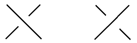
Given a tangle $T$, let $\mathcal{D}(T)$ denote the set of directed arcs. For $\mathsf{a}\in\mathcal{D}(T)$, let $\mathsf{a}^{-1}$ denote the direct arc obtained from $\mathsf{a}$ by reversing the direction. A map $\rho:\mathcal{D}(T)\to G$ is called a representation of $T$ if $\rho(\mathsf{a}^{-1})=\rho(\mathsf{a})^{-1}$ for all $\mathsf{a}$ and $\rho(\mathsf{c})=\rho(\mathsf{a})\lrcorner\rho(\mathsf{b})$ for any $\mathsf{a},\mathsf{b},\mathsf{c}$ forming a crossing as

To present such $\rho$, it suffices to choose a direction for each arc and label the arc with an element of $G$. In view of Wirtinger presentation, $\rho$ can be identified with a genuine representation $\tilde{\rho}:\pi_{1}(B\setminus T)\to G$.

Call $\rho$ reducible, irreducible, abelian, etc, if respectively $\tilde{\rho}$ is. In particular, call $\rho$ NR if it is nonabelian and reducible.

Let $\mathcal{R}(T)$ denote the set of all representations of $T$. Given $\rho\in\mathcal{R}(T)$ and $\mathbf{c}\in G$, let $\mathbf{c}\lrcorner\rho\in\mathcal{R}(T)$ send $\mathsf{a}$ to $\mathbf{c}\lrcorner\rho(\mathsf{a})$. Call $\rho,\rho^{\prime}\in\mathcal{R}(T)$ conjugate and denote $\rho\sim\rho^{\prime}$ if $\rho^{\prime}=\mathbf{c}\lrcorner\rho$ for some $\mathbf{c}$. Let $\mathcal{X}(T)=\mathcal{R}(T)/\sim$, the set of conjugacy classes of representations of $T$; let $\mathcal{X}^{\rm red}(T)$, $\mathcal{X}^{\rm irr}(T)$ respectively denote the set of conjugacy classes of reducible and irreducible representations.

If $S$ is a subtangle of $T$, and $\rho\in\mathcal{R}(T)$, then the composite map $\mathcal{D}(S)\to\mathcal{D}(T)\stackrel{{\scriptstyle\rho}}{{\to}}G$ is a representation of $S$, which is denoted by $\rho|_{S}$.

Figure 1: From left to right: a tangle $T$ in $\mathcal{T}_{2}^{2}$; $N(T)$; $D(T)$; $T_{1}\ast T_{2}$; $T_{1}+T_{2}$.

Let $\mathcal{T}_{2}^{2}$ denote the set of four-end tangles of the form shown at leftmost in Figure 1. To each $T\in\mathcal{T}_{2}^{2}$ are associated two links, called the numerator $N(T)$ and the denominator $D(T)$. Defined on $\mathcal{T}_{2}^{2}$ are the vertical composition $\ast$ and the horizontal composition $+$.

Figure 2: Left: the tangle $[1]$. Right: $[-1]$.

A tangle $T\in\mathcal{T}_{2}^{2}$ is called arborescent if it can be constructed from copies of $[\pm 1]$ (see Figure 2) via repeatedly applying $\ast$ and $+$. Let $\mathcal{T}_{\rm ar}$ denote the set of arborescent tangles. An arborescent knot is a knot of the form $N(T)$ or $D(T)$ for some $T\in\mathcal{T}_{\rm ar}$.

For $k\neq 0$, the horizontal composite of $|k|$ copies of $[1]$ (resp. $[-1]$) is denoted by $[k]$ if $k>0$ (resp. $k<0$), and the vertical composite of $|k|$ copies of $[1]$ (resp. $[-1]$) is denoted by $[1/k]$ if $k>0$ (resp. $k<0$). Given $p/q\in\mathbb{Q}$, if a continued fraction of $p/q$ is

$$k_{s}+1/(k_{s-1}+\cdots+1/k_{1})\cdots),$$

then the associated rational tangle is defined as

$$[p/q]=[[k_{1}],\ldots,[k_{m}]]=\begin{cases}(\cdots([k_{1}]\ast[1/k_{2}])+\cdots)+[k_{m}],&2\nmid m\\ (\cdots([1/k_{1}]+[k_{2}])\ast\cdots)+[k_{m}],&2\mid m\end{cases}.$$

When speaking of $T\in\mathcal{T}_{\rm ar}$, we usually assume that an order of repeated horizontal/vertical compositions of rational tangles has been chosen. Call the arborescent subtangles appearing in the compositions subsequent to $T$. For example, if $R_{1},\ldots,R_{6}$ are rational tangles, then

$$T=((R_{1}+R_{2})+(R_{3}\ast R_{4}))\ast(R_{5}+R_{6})\in\mathcal{T}_{\rm ar},$$

and $R_{3}$, $R_{3}\ast R_{4}$, $(R_{1}+R_{2})+(R_{3}\ast R_{4})$, $R_{5}$, etc. are subsequent to $T$.

3 Methodology

Suppose $T\in\mathcal{T}_{\rm ar}$. Let $T^{{\rm nw}}$, $T^{{\rm ne}}$, $T^{{\rm sw}}$, $T^{{\rm se}}$ respectively denote the arcs at the northwest, northeast, southwest, southeast end of $T$, all directed outward.

For $t\in\mathbb{C}$, let

$$\mathcal{R}_{t}(T)=\{\rho\in\mathcal{R}(T)\colon\rho(\mathsf{a})\in G(t)\ \text{for\ all\ }\mathsf{a}\in\mathcal{D}(T)\}.$$

Given $\rho\in\mathcal{R}_{t}(T)$ and $\o \in\{{\rm nw},{\rm ne},{\rm sw},{\rm se}\}$, let $\mathbf{x}^{\o }=\mathbf{x}^{\o }_{\rho}=\rho(T^{\o })$. Put

$$\mathbf{z}_{\rho}=\mathbf{x}^{{\rm nw}}\mathbf{x}^{{\rm ne}},\qquad\dot{\mathbf{z}}_{\rho}=\mathbf{x}^{{\rm ne}}\mathbf{x}^{{\rm se}},\qquad\grave{\mathbf{z}}_{\rho}=\mathbf{x}^{{\rm nw}}\mathbf{x}^{{\rm se}},\qquad\acute{\mathbf{z}}_{\rho} =\mathbf{x}^{{\rm sw}}\mathbf{x}^{{\rm ne}}.$$

Furthermore, we associate

$$u =u(\rho)={\rm tr}(\mathbf{z}_{\rho}),\qquad\dot{u}=\dot{u}(\rho)={\rm tr}(\dot{\mathbf{z}}_{\rho}),$$

$$\grave{u} =\grave{u}(\rho)={\rm tr}(\grave{\mathbf{z}}_{\rho}),\qquad\acute{u}=\acute{u}(\rho)={\rm tr}(\acute{\mathbf{z}}_{\rho}),$$

$$\hskip 51.21495pt\check{u}=\check{u}(\rho)=\grave{u}-\acute{u}.$$

We mainly consider $\rho\in\mathcal{R}_{t}(T)$ for a fixed $t$. The trace-free case, i.e. the one with $t=0$, had been thoroughly investigated in [3].

3.1 Representations of rational tangles revisited

It is worth clarifying some facts about representations of rational tangles.

Figure 3: The rational tangle $[[k_{1}],\ldots,[k_{m}]]$; the case $m$ is odd (resp. even) is shown at left (resp. right). The $x^{(j)}$’s, $y^{(j)}$’s are directed arcs.

In this subsection, suppose $T$ is a rational tangle, and let $x^{(j)},y^{(j)}\in\mathcal{D}(T)$ denote the directed arcs as shown in Figure 3.

Given $\rho\in\mathcal{R}_{t}(T)$, let $\mathbf{x}^{(j)}=\rho(x^{(j)})$, $\mathbf{y}^{(j)}=\rho(y^{(j)})$; let $\mathbf{x}=\mathbf{x}^{(0)}$, $\mathbf{y}=\mathbf{y}^{(0)}$, and $r={\rm tr}(\mathbf{x}\mathbf{y})$. As explained in [4, Section 3.1], each of $\mathbf{x}^{(j)}$ and $\mathbf{y}^{(j)}$ can be written as a $\mathbb{Z}[t,r]$-linear combination of $\mathbf{e}$, $\mathbf{x}$, $\mathbf{y}$, $\mathbf{x}\mathbf{y}$. Hence $\rho$ is determined by $\mathbf{x}$, $\mathbf{y}$; denote $\rho$ as $\rho^{\mathbf{x}}_{\mathbf{y}}$. Clearly, $u(\rho),\dot{u}(\rho),\acute{u}(\rho),\grave{u}(\rho)$ are all determined by $t,r$. Let $u(t,r)=u_{T}(t,r)=u(\rho)\in\mathbb{Z}[t,r]$, etc.

Remark 3.1.

Recall [4, Lemma 3.1] that $\mathbf{y}$ can be written as a word in $\mathbf{x}^{\rm nw},\mathbf{x}^{\rm ne},\mathbf{x}^{\rm sw},\mathbf{x}^{\rm se}$. Remembering $\mathbf{x}^{\rm nw}\in\{\mathbf{x}^{\pm 1}\}$ and $\mathbf{x}^{\rm se}=(\mathbf{x}^{\rm sw}\mathbf{x}^{\rm nw}\mathbf{x}^{\rm ne})^{-1}$, we see that $\rho$ is reducible if and only if $(\mathbf{x}^{\rm nw},\mathbf{x}^{\rm ne},\mathbf{x}^{\rm sw})$ is.

Lemma 3.2.

Suppose $r\neq 2,t^{2}-2$. Given $\mathbf{a}^{\rm nw},\mathbf{a}^{\rm ne},\mathbf{a}^{\rm sw}\in G(t)$ with

$${\rm tr}(\mathbf{a}^{\rm nw}\mathbf{a}^{\rm ne}) =u(t,r),\qquad {\rm tr}(\mathbf{a}^{\rm nw}\mathbf{a}^{\rm sw})=\dot{u}(t,r),$$

$${\rm tr}(\mathbf{a}^{\rm sw}\mathbf{a}^{\rm ne}) =\acute{u}(t,r),\qquad {\rm tr}(\mathbf{a}^{\rm sw}\mathbf{a}^{\rm nw}\mathbf{a}^{\rm ne})=t,$$

there exists a unique pair $(\mathbf{x},\mathbf{y})\in G(t)^{2}$ such that ${\rm tr}(\mathbf{x}\mathbf{y})=r$ and $\rho^{\mathbf{x}}_{\mathbf{y}}(T^{\o })=\mathbf{a}^{\o }$ for all $\o \in\{{\rm nw},{\rm ne},{\rm sw}\}$.

Proof.

By Lemma 2.3 (a), there exists an irreducible pair $(\mathbf{u},\mathbf{v})\in G(t)^{2}$ with ${\rm tr}(\mathbf{u}\mathbf{v})=r$. By Remark 3.1, $(\rho^{\mathbf{u}}_{\mathbf{v}}(T^{\rm nw}),\rho^{\mathbf{u}}_{\mathbf{v}}(T^{\rm ne}),\rho^{\mathbf{u}}_{\mathbf{v}}(T^{\rm sw}))$ is irreducible. Due to the equalities on traces, there exists $\mathbf{c}\in G$ such that $\mathbf{c}\lrcorner\rho^{\mathbf{u}}_{\mathbf{v}}(T^{\o })=\mathbf{a}^{\o }$ for $\o \in\{{\rm nw},{\rm ne},{\rm sw}\}.$ Then $(\mathbf{x},\mathbf{y})=(\mathbf{c}\lrcorner\mathbf{u},\mathbf{c}\lrcorner\mathbf{v})$ fulfills the required conditions.

The uniqueness has been explained in Remark 3.1. ∎

3.2 Representations of arborescent tangles

The basic step is, for $T=T_{1}\ast T_{2}$ or $T=T_{1}+T_{2}$, to carefully analyze the relationship between $\mathcal{R}(T)$ and $\mathcal{R}(T_{1}),\mathcal{R}(T_{2})$, in all possible cases. The composition formulas in Lemma 3.6 will be important.

By Lemma 2.2 (ii), $\mathbf{z}=-\mathbf{e}$ is impossible, unless $t=0$.

When $t\neq 0$, in principle we can deal with the following cases separately: (i) $u\neq 2,t^{2}-2$; (ii) $\mathbf{z}=\mathbf{e}$; (iii) $u=2$ but $\mathbf{z}\neq\mathbf{e}$, in which case, up to conjugacy we may assume $\mathbf{z}=\mathbf{p}$; (iv) $u=t^{2}-2\neq\pm 2$. In practice, each of the cases (ii)–(iv) has diverse possibilities and needs further investigation.

We focus on (i), the generic case, and allow $t=0$.

When $u=\lambda+\lambda^{-1}\neq\pm 2,t^{2}-2$, up to conjugacy we may assume $\mathbf{z}=\mathbf{d}(\lambda)$, then by Lemma 2.1 (a), there exist $\mu,\nu$ such that

$$\mathbf{x}^{\rm nw} =\mathbf{h}^{\lambda}_{t}(-\lambda\nu),\qquad \mathbf{x}^{\rm ne} =\mathbf{h}^{\lambda}_{t}(\nu),$$

$$(\mathbf{x}^{\rm sw})^{-1} =\mathbf{h}^{\lambda}_{t}(-\lambda\mu),\qquad (\mathbf{x}^{\rm se})^{-1} =\mathbf{h}^{\lambda}_{t}(\mu).$$

An application of (1) leads to

$$(u+2)\dot{u} =2t^{2}+(u+2-t^{2})(\nu\mu^{-1}+\nu^{-1}\mu),$$ (2)

$$(u+2)\grave{u} =2t^{2}-(u+2-t^{2})(\lambda\nu\mu^{-1}+\lambda^{-1}\nu^{-1}\mu),$$ (3)

$$(u+2)\acute{u} =2t^{2}-(u+2-t^{2})(\lambda^{-1}\nu\mu^{-1}+\lambda\nu^{-1}\mu),$$ (4)

$$(u+2)\check{u} =(u+2-t^{2})(\lambda-\lambda^{-1})(\nu^{-1}\mu-\nu\mu^{-1}).$$ (5)

The first three equations imply

$$\grave{u}+\acute{u}+u\dot{u}=2t^{2};$$ (6)

it follows from (2), (5) that

$$\frac{\mu}{\nu} =\frac{(u+2)(\dot{u}+\check{u}/(\lambda-\lambda^{-1}))-2t^{2}}{2(u+2-t^{2})},$$ (7)

$$\frac{\nu}{\mu} =\frac{(u+2)(\dot{u}-\check{u}/(\lambda-\lambda^{-1}))-2t^{2}}{2(u+2-t^{2})}.$$ (8)

The trivial identity $(\mu/\nu)\cdot(\nu/\mu)=1$ gives rise to

$$\check{u}^{2}=(u-2)(\dot{u}-2)\big((u+2)(\dot{u}+2)-4t^{2}\big).$$ (9)

Remark 3.3.

The equation (6) implies that $u,\dot{u},\check{u}$ determine $\grave{u},\acute{u}$, so as to determine $(\mathbf{x}^{\rm nw},\mathbf{x}^{\rm ne},\mathbf{x}^{\rm sw},\mathbf{x}^{\rm se})$ up to conjugacy.

Being polynomial identities, (6), (9) actually hold without the assumption $u\neq\pm 2,t^{2}-2$.

Define an equivalence relation $\sim$ on $\mathbb{C}^{\ast}\times\mathbb{C}^{\ast}$ by $(\mu,\nu)\sim(\mu^{-1},\nu^{-1})$. Let

$$\mathcal{E}=\{(\mu,\nu)\in\mathbb{C}^{\ast}\times\mathbb{C}^{\ast}\colon\mu\neq\pm 1\ \text{or\ }\nu\neq\pm 1\}/\sim.$$

Partially defined on $\mathcal{E}$ are two operations:

$$(\mu,\nu)\circ_{h}(\mu,\nu^{\prime}) =(\mu,\nu\nu^{\prime}),\qquad \mu\neq\pm 1;$$

$$(\mu,\nu)\circ_{v}(\mu^{\prime},\nu) =(\mu\mu^{\prime},\nu),\qquad \nu\neq\pm 1.$$

When $u\neq\pm 2,t^{2}-2$, define $\mathfrak{v}(\rho)=(\mu,\lambda)\in\mathcal{E}$ by taking $\lambda$ with $\lambda+\lambda^{-1}=u$ and putting

$$\mu=\frac{(u+2)(\dot{u}+\check{u}/(\lambda-\lambda^{-1}))-2t^{2}}{2(u+2-t^{2})}\stackrel{{\scriptstyle(\ref{eq:identity-3})}}{{=}}\Big(\frac{(u+2)(\dot{u}-\check{u}/(\lambda-\lambda^{-1}))-2t^{2}}{2(u+2-t^{2})}\Big)^{-1}.$$ (10)

Alternatively, up to conjugacy we may assume $\mathbf{z}=\mathbf{d}(\lambda)$, then by Lemma 2.1 (a),

$$\mathbf{x}^{\rm nw} =\mathbf{h}^{\lambda}_{t}(-\lambda\gamma),\qquad \mathbf{x}^{\rm ne} =\mathbf{h}^{\lambda}_{t}(\gamma),$$

$$(\mathbf{x}^{\rm sw})^{-1} =\mathbf{h}^{\lambda}_{t}(-\lambda\gamma^{\prime}),\qquad (\mathbf{x}^{\rm se})^{-1} =\mathbf{h}^{\lambda}_{t}(\gamma^{\prime})$$

for some $\gamma,\gamma^{\prime}$; we put $\mu=\gamma^{\prime}/\gamma$. It follows from (10) that

$$\dot{u} =\frac{2t^{2}+(u+2-t^{2})(\mu+\mu^{-1})}{u+2},$$ (11)

$$\check{u} =\frac{(u+2-t^{2})(\lambda-\lambda^{-1})(\mu-\mu^{-1})}{u+2}.$$ (12)

When $\dot{u}\neq\pm 2,t^{2}-2$, define $\mathfrak{h}(\rho)=(\eta,\nu)\in\mathcal{E}$ by taking $\eta$ with $\eta+\eta^{-1}=\dot{u}$ and putting

$$\nu=\frac{(\dot{u}+2)(u+\check{u}/(\eta-\eta^{-1}))-2t^{2}}{2(\dot{u}+2-t^{2})}\stackrel{{\scriptstyle(\ref{eq:identity-3})}}{{=}}\Big(\frac{(\dot{u}+2)(u-\check{u}/(\eta-\eta^{-1}))-2t^{2}}{2(\dot{u}+2-t^{2})}\Big)^{-1}.$$ (13)

Alternatively, up to conjugacy we may assume $\dot{\mathbf{z}}=\mathbf{d}(\eta)$, then by Lemma 2.1 (a),

$$\mathbf{x}^{\rm ne} =\mathbf{h}^{\eta}_{t}(-\eta\gamma),\qquad \mathbf{x}^{\rm se} =\mathbf{h}^{\eta}_{t}(\gamma),$$

$$(\mathbf{x}^{\rm nw})^{-1} =\mathbf{h}^{\eta}_{t}(-\eta\gamma^{\prime}),\qquad (\mathbf{x}^{\rm sw})^{-1} =\mathbf{h}^{\eta}_{t}(\gamma^{\prime})$$

for some $\gamma,\gamma^{\prime}$; we put $\nu=\gamma/\gamma^{\prime}$. It follows from (13) that

$$u =\frac{2t^{2}+(\dot{u}+2-t^{2})(\nu+\nu^{-1})}{\dot{u}+2},$$ (14)

$$\check{u} =\frac{(\dot{u}+2-t^{2})(\eta-\eta^{-1})(\nu-\nu^{-1})}{\dot{u}+2}.$$ (15)

By definition, the following properties are immediate:

$$\mathfrak{h}(\rho_{1}+\rho_{2}) =\mathfrak{h}(\rho_{1})\circ_{h}\mathfrak{h}(\rho_{2}),$$ (16)

$$\mathfrak{v}(\rho_{1}\ast\rho_{2}) =\mathfrak{v}(\rho_{1})\circ_{v}\mathfrak{v}(\rho_{2}).$$ (17)

Example 3.4.

Let $T$ be a rational tangle, and $\rho\in\mathcal{R}_{t}^{\rm irr}(T)$. Write $\dot{u}=\eta+\eta^{-1}$, $u=\mu+\mu^{-1}$.

When $T=[1]$, up to conjugacy we may assume $(\mathbf{x}^{\rm nw})^{-1}=\mathbf{h}_{t}^{\eta}(-\eta)$, $(\mathbf{x}^{\rm sw})^{-1}=\mathbf{h}_{t}^{\eta}(1)$, then $\mathbf{x}^{\rm se}=\mathbf{h}_{t}^{\eta}(-\eta)$, and it is easy to see $\mathfrak{h}(\rho)=(\eta,-\eta)$. Alternatively, up to conjugacy we may also assume $(\mathbf{x}^{\rm sw})^{-1}=\mathbf{h}_{t}^{\mu}(-\mu)$, $(\mathbf{x}^{\rm se})^{-1}=\mathbf{h}_{t}^{\mu}(1)$, then $\mathbf{x}^{\rm nw}=\mathbf{h}_{t}^{\mu}(1)$, and it is easy to see $\mathfrak{v}(\rho)=(-\mu,\mu)$.

For $r=\zeta+\zeta^{-1}$ and $n\in\mathbb{Z}$, put $\theta_{n}(r)=\zeta^{n}+\zeta^{-n}$,

$$\omega_{n}(r) =\begin{cases}(\zeta^{n}-\zeta^{-n})/(\zeta-\zeta^{-1}),&\zeta\neq\pm 1\\ n\zeta^{n-1},&\zeta\in\{\pm 1\}\end{cases},$$

$$\alpha_{n}(r) =\frac{2t^{2}+(-1)^{n}(r+2-t^{2})\theta_{n}(r)}{r+2}.$$

In particular,

$$\alpha_{\pm 2}(r) =r^{2}-2+t^{2}(2-r)=2+(r-2)(r+2-t^{2}),$$

$$\alpha_{\pm 3}(r) =3r-r^{3}+t^{2}(r-1)^{2}=2-(r+2-t^{2})(r-1)^{2}.$$

When $T=[k]$, repeatedly applying (16), we obtain $\mathfrak{h}(\rho)=(\eta,(-\eta)^{k})$, so

$$u=\alpha_{k}(\dot{u}),\qquad\check{u}=(-1)^{k}(\dot{u}-2)(\dot{u}+2-t^{2})\omega_{k}(\dot{u}).$$ (18)

When $T=[1/k]$, repeatedly applying (17), we obtain $\mathfrak{v}(\rho)=((-\mu)^{k},\mu)$, so

$$\dot{u}=\alpha_{k}(u),\qquad\check{u}=(-1)^{k}(u-2)(u+2-t^{2})\omega_{k}(u).$$ (19)

In general case, one may refer to the formulas given in [4, Section 3.1], which were expressed in terms of the polynomials $\psi_{j}(n)$.

Remark 3.5.

In the case $t=0$, things can be dramatically simplified. It is easy to see that $\mathfrak{h}(\rho)=\mathfrak{v}(\rho)=(\mu,\nu)$, with

$$\dot{u}=\mu+\mu^{-1},\qquad u=\nu+\nu^{-1},\qquad\check{u}=(\mu-\mu^{-1})(\nu-\nu^{-1}).$$

When $T=[p/q]=[[k_{1}],\ldots,[k_{m}]]$, as shown in [3, Example 4.4], up to conjugacy, each $\rho\in\mathcal{R}_{0}^{\rm irr}([p/q])$ is determined by $\mathfrak{v}(\rho)=\mathfrak{h}(\rho)=(\alpha,\beta)$ with

$$(-\alpha)^{p}+(-\beta)^{q}=0,$$

through $r=\alpha^{-\tilde{q}}\beta^{\tilde{p}}+\alpha^{\tilde{q}}\beta^{-\tilde{p}}$, where $\tilde{p}/\tilde{q}=[[k_{2},\ldots,k_{m}]]^{(-1)^{m-1}}$.

Given $b_{1},c_{1},b_{2},c_{2}\in\mathbb{C}$ and $a\neq 2,t^{2}-2$, put

$$g_{a}(b_{1},c_{1};b_{2},c_{2}) =\frac{(a+2)b_{1}b_{2}+2t^{2}(2-b_{1}-b_{2})+c_{1}c_{2}/(a-2)}{2(a+2-t^{2})},$$ (20)

$$h_{a}(b_{1},c_{1};b_{2},c_{2}) =\frac{(a+2)(b_{1}c_{2}+b_{2}c_{1})-2t^{2}(c_{1}+c_{2})}{2(a+2-t^{2})}.$$ (21)

Lemma 3.6.

Suppose $T=T_{1}\ast T_{2}$ or $T=T_{1}+T_{2}$. Given $\rho\in\mathcal{R}_{t}(T)$, let $u=u(\rho)$, $\dot{u}=\dot{u}(\rho)$, and let $u_{i}=u(\rho|_{T_{i}})$, $\dot{u}_{i}=\dot{u}(\rho|_{T_{i}})$, $\check{u}_{i}=\check{u}(\rho|_{T_{i}})$, $i=1,2$.

1. If $T=T_{1}\ast T_{2}$ and $u\neq 2,t^{2}-2$, then

   $$\dot{u}(\rho)=g_{u}(\dot{u}_{1},\check{u}_{1};\dot{u}_{2},\check{u}_{2}),\qquad\check{u}(\rho)=h_{u}(\dot{u}_{1},\check{u}_{1};\dot{u}_{2},\check{u}_{2}).$$

2. If $T=T_{1}+T_{2}$ and $\dot{u}\neq 2,t^{2}-2$, then

   $$u(\rho)=g_{\dot{u}}(u_{1},\check{u}_{1};u_{2},\check{u}_{2}),\qquad\check{u}(\rho)=h_{\dot{u}}(u_{1},\check{u}_{1};u_{2},\check{u}_{2}).$$

Proof.

We only prove (i); the proof for (ii) is similar.

Suppose $u\neq-2$. Suppose $\mathfrak{v}(\rho|_{T_{i}})=(\mu_{i},\lambda)$, $i=1,2$, with $\lambda+\lambda^{-1}=u$. Then by (10),

$$\mu_{i}^{\pm 1}=\frac{1}{2(u+2-t^{2})}\left((u+2)\left(\dot{u}_{i}\pm\frac{\check{u}_{i}}{\lambda-\lambda^{-1}}\right)-2t^{2}\right),$$

and by (17), $\mathfrak{v}(\rho)=(\mu_{1}\mu_{2},\lambda)$. By direct computation,

$$\dot{u} =\frac{2t^{2}+(u+2-t^{2})(\mu_{1}\mu_{2}+\mu_{1}^{-1}\mu_{2}^{-1})}{u+2}=g_{u}(\dot{u}_{1},\check{u}_{1};\dot{u}_{2},\check{u}_{2}),$$

$$\check{u} =\frac{(u+2-t^{2})(\lambda-\lambda^{-1})(\mu_{1}^{-1}\mu_{2}^{-1}-\mu_{1}\mu_{2})}{u+2}=h_{u}(\dot{u}_{1},\check{u}_{1};\dot{u}_{2},\check{u}_{2}).$$

By continuity, the assertion also holds when $u=-2$ (in which case $t\neq 0$, due to $u\neq t^{2}-2$). ∎

For $a,b,c\in\mathbb{C}$, let $\mathcal{X}_{t;a,b}^{c}(T)$ denote the set of conjugacy classes of representations $\rho\in\mathcal{R}_{t}(T)$ with $u(\rho)=a$, $\dot{u}(\rho)=b$, $\check{u}(\rho)=c$.

Corollary 3.7.

Suppose $a,b,c\in\mathbb{C}$.

1. When $a\neq 2,t^{2}-2$, the map $\rho\mapsto(\rho|_{T_{1}},\rho|_{T_{2}})$ induces a bijection

   $$\mathcal{X}_{t;a,b}^{c}(T_{1}\ast T_{2})\cong{\bigcup}_{(b_{1},c_{1};b_{2},c_{2})\in g_{a}^{-1}(b)\cap h_{a}^{-1}(c)}\mathcal{X}_{t;a,b_{1}}^{c_{1}}(T_{1})\times\mathcal{X}_{t;a,b_{2}}^{c_{2}}(T_{2}).$$

2. When $b\neq 2,t^{2}-2$, the map $\rho\mapsto(\rho|_{T_{1}},\rho|_{T_{2}})$ induces a bijection

   $$\mathcal{X}_{t;a,b}^{c}(T_{1}+T_{2})\cong{\bigcup}_{(a_{1},c_{1};a_{2},c_{2})\in g_{b}^{-1}(a)\cap h_{b}^{-1}(c)}\mathcal{X}_{t;a_{1},b}^{c_{1}}(T_{1})\times\mathcal{X}_{t;a_{2},b}^{c_{2}}(T_{2}).$$

Proof.

We only prove (i); the proof for (ii) is similar.

Given $\rho_{i}\in\mathcal{R}_{t}(T_{i})$ with $u(\rho_{i})=a$, $\dot{u}(\rho_{i})=b_{i}$, $\check{u}(\rho_{i})=c_{i}$, $i=1,2$, due to

$${\rm tr}(\rho_{1}(T_{1}^{\rm sw})\rho_{1}(T_{1}^{\rm se}))={\rm tr}(\rho_{2}(T_{2}^{\rm nw})^{-1}\rho_{2}(T_{2}^{\rm ne})^{-1})=a\neq 2,t^{2}-2,$$

by Lemma 2.3 (i), there exists $\mathbf{c}\in G$ such that $\mathbf{c}\lrcorner\rho_{1}(T_{1}^{\rm sw})=\rho_{2}(T_{2}^{\rm nw})^{-1}$ and $\mathbf{c}\lrcorner\rho_{1}(T_{1}^{\rm se})=\rho_{2}(T_{2}^{\rm ne})^{-1}.$ We can glue $\mathbf{c}\lrcorner\rho_{1}$ and $\rho_{2}$ into $\rho\in\mathcal{R}_{t}(T)$. By Lemma 3.6 (i), $\dot{u}(\rho)=g_{a}(b_{1},c_{1};b_{2},c_{2})$, $\check{u}(\rho)=h_{a}(b_{1},c_{1};b_{2},c_{2})$.

In this way, we construct the inverse to the map

$$\mathcal{X}_{t;a,b}^{c}(T_{1}\ast T_{2})\to{\bigcup}_{(b_{1},c_{1};b_{2},c_{2})\in g_{a}^{-1}(b)\cap h_{a}^{-1}(c)}\mathcal{X}_{t;a,b_{1}}^{c_{1}}(T_{1})\times\mathcal{X}_{t;a,b_{2}}^{c_{2}}(T_{2})$$

induced by $\rho\mapsto(\rho|_{T_{1}},\rho|_{T_{2}})$. ∎

3.3 Reducible representations

When $S=S_{1}+S_{2}$ or $S=S_{1}\ast S_{2}$, possibly $\rho|_{S_{1}}$ or $\rho|_{S_{2}}$ is reducible for some $\rho\in\mathcal{R}^{\rm irr}(S)$. So it is worth taking $\mathcal{R}^{\rm red}(T)$ into account for $T\in\mathcal{T}_{\rm ar}$.

Suppose $\rho\in\mathcal{R}_{t}(T)$ is NR, so that $t\neq\pm 2$. Fix $\kappa\neq\pm 1$ with $\kappa+\kappa^{-1}=t$. Up to conjugacy we may assume ${\rm Im}(\rho)\subset\mathsf{T}_{+}$. Assume that for $\mathsf{a}\in\mathcal{D}(T)$,

$$\rho(\mathsf{a})=\mathbf{u}_{\kappa}(\xi_{\mathsf{a}})^{\epsilon_{\mathsf{a}}}=\mathbf{u}_{\kappa^{\epsilon_{\mathsf{a}}}}(\epsilon_{\mathsf{a}}\xi_{\mathsf{a}}),\qquad\xi_{\mathsf{a}}\in\mathbb{C},\quad\epsilon_{\mathsf{a}}\in\{\pm 1\}.$$

Figure 4:

When $\mathsf{a},\mathsf{b},\mathsf{c}$ form a positive crossing (as shown in Figure 4, left), $\rho(\mathsf{c})=\rho(\mathsf{a})\lrcorner\rho(\mathsf{b})$, i.e. $\mathbf{u}_{\kappa}(\xi_{\mathsf{c}})^{\epsilon_{\mathsf{c}}}=\mathbf{u}_{\kappa}(\xi_{\mathsf{a}})^{\epsilon_{\mathsf{a}}}\lrcorner(\mathbf{u}_{\kappa}(\xi_{\mathsf{b}})^{\epsilon_{\mathsf{b}}})$. Comparing the $(1,1)$- and $(1,2)$-entries, we obtain

$$\kappa^{\epsilon_{\mathsf{c}}}=\kappa^{\epsilon_{\mathsf{b}}},\qquad\epsilon_{\mathsf{c}}\xi_{\mathsf{c}}=\kappa^{2\epsilon_{\mathsf{a}}}\epsilon_{\mathsf{b}}\xi_{\mathsf{b}}+\kappa^{\epsilon_{\mathsf{a}}}(\kappa^{-\epsilon_{\mathsf{b}}}-\kappa^{\epsilon_{\mathsf{b}}})\epsilon_{\mathsf{a}}\xi_{\mathsf{a}},$$

which imply

$$\xi_{\mathsf{c}}=\big(1-\kappa^{2\epsilon_{\mathsf{a}}}\big)\xi_{\mathsf{a}}+\kappa^{2\epsilon_{\mathsf{a}}}\xi_{\mathsf{b}}.$$ (22)

Similarly, when $\mathsf{a},\mathsf{b},\mathsf{c}$ form a negative crossing, one has

$$\xi_{\mathsf{c}}=\big(1-\kappa^{-2\epsilon_{\mathsf{a}}}\big)\xi_{\mathsf{a}}+\kappa^{-2\epsilon_{\mathsf{a}}}\xi_{\mathsf{b}}.$$ (23)

Orient the components of $T$ (as a $1$-submanifold of a $3$-ball), so that a direction is chosen for each of its arcs. Numerate the crossings of $T$ as $\mathfrak{c}_{1},\ldots,\mathfrak{c}_{n}$, and the directed arcs as $x_{1},\ldots,x_{n+2}$. Construct $Q_{T}=(q_{ij})_{n\times(n+2)}$ as follows: for each $i$, if $\mathfrak{c}_{i}$ is formed by $\mathsf{a}=x_{k_{1}}$, $\mathsf{b}=x_{k_{2}}$, $\mathsf{c}=x_{k_{3}}$, then let

$$q_{i,k_{1}}=1-\kappa^{2\varepsilon_{i}},\qquad q_{i,k_{2}}=\kappa^{2\varepsilon_{i}},\qquad q_{i,k_{3}}=-1,$$

where $\varepsilon_{i}=\epsilon_{\mathsf{a}}$ (resp. $\varepsilon_{i}=-\epsilon_{\mathsf{a}}$) if $\mathfrak{c}_{i}$ is positive (resp. negative); let $q_{i,j}=0$ for $j\notin\{k_{1},k_{2},k_{3}\}$. By (22), (23), we have $Q_{T}(\xi_{x_{1}},\ldots,\xi_{x_{n+2}})=0.$

Remark 3.8.

The matrix $Q_{T}$ identifies with the $Q_{T}$ defined in [5, Section 4.2], under which $\kappa^{2\varepsilon_{i}}$ corresponds to $\tau_{\overline{i}}^{\epsilon}$.

For $S\in\mathcal{T}_{\rm ar}$, define its fraction $f(S)\in\mathbb{Q}\cup\{\infty\}$ by setting $f(S)=p/q$ if $S=[p/q]$, and recursively,

$$f(S_{1}+S_{2})=f(S_{1})+f(S_{2}),\qquad\frac{1}{f(S_{1}\ast S_{2})}=\frac{1}{f(S_{1})}+\frac{1}{f(S_{2})},$$

with the convention $\infty+\infty=\infty$, $1/0=\infty$, $1/\infty=0$.

Let $\xi^{\rm nw}=\xi_{T^{\rm nw}}$, etc. As elucidated in [5, Section 4], if $T$ is generic, in the sense that $f(S)\neq 0,\infty$ for all tangles subsequent to $T$, then for each arc $x$, there exists $b^{x},c^{x}\in\mathbb{Q}(\kappa)$ such that

$$\xi_{x}=(1-b^{x})\xi^{\rm nw}+b^{x}\xi^{\rm ne}=(1-c^{x})\xi^{\rm nw}+c^{x}\xi^{\rm sw}.$$

In particular, there exist $b^{\rm sw},b^{\rm se},c^{\rm ne},c^{\rm se}\in\mathbb{Q}(\kappa)$ determined by $T$ such that

$$\left(\begin{array}[]{cc}\xi^{\rm sw}\\ \xi^{\rm se}\end{array}\right) =F_{v}^{T}\left(\begin{array}[]{cc}\xi^{\rm nw}\\ \xi^{\rm ne}\end{array}\right),\qquad \text{with}\quad F_{v}^{T}=\left(\begin{array}[]{cc}1-b^{\rm sw}&b^{\rm sw}\\ 1-b^{\rm se}&b^{\rm se}\end{array}\right),$$ (30)

$$\left(\begin{array}[]{cc}\xi^{\rm ne}\\ \xi^{\rm se}\end{array}\right) =F_{h}^{T}\left(\begin{array}[]{cc}\xi^{\rm nw}\\ \xi^{\rm sw}\end{array}\right),\qquad \text{with}\quad F_{h}^{T}=\left(\begin{array}[]{cc}1-c^{\rm ne}&c^{\rm ne}\\ 1-c^{\rm se}&c^{\rm se}\end{array}\right).$$ (37)

When $T$ is not generic, the situation is obscure, and more efforts are required.

When $\kappa^{2}=-1$, i.e. $t=0$, we can recursively show $b^{\rm sw}=-1/f(T)$, $c^{\rm ne}=-f(T)$. The equations (30), (37) are consistent with the following result presented in [3, Page 110 and 112]: If $\rho\in\mathcal{R}_{0}^{\rm red}(T)$, so that $\dot{u}=2\alpha$, $u=2\beta$ with $\alpha,\beta\in\{\pm 1\}$, then

$$(\mathbf{x}^{\rm ne},\mathbf{x}^{\rm se}) =-\beta(\mathbf{x}^{\rm nw},\mathbf{x}^{\rm sw})C_{\alpha}(f(T)),$$ (38)

$$(\mathbf{x}^{\rm sw},\mathbf{x}^{\rm se}) =-\alpha(\mathbf{x}^{\rm nw},\mathbf{x}^{\rm ne})C_{\beta}(1/f(T)),$$ (39)

where for $\gamma\in\{\pm 1\}$ and $c\in\mathbb{C}$, we put

$$C_{\gamma}(c)=\left(\begin{array}[]{cc}1+c&-\gamma c\\ \gamma c&1-c\end{array}\right).$$

3.4 On representations of arborescent knots

The link $N(T)$ is equivalent to $D(T^{\prime})$, where $T^{\prime}$ is obtained from rotating $T$ by $\pi/2$. Thus, we may just pay attention to knots of the form $K=D(T)$. Evidently, representations of $K$ identify with $\rho\in\mathcal{R}(T)$ such that $\dot{\mathbf{z}}_{\rho}=\mathbf{e}$.

When $S=S_{1}+S_{2}$ (resp. $S=S_{1}\ast S_{2}$), call $\rho\in\mathcal{R}_{t}(S)$ non-degenerate if $\dot{u}(\rho)\neq 2,t^{2}-2$ (resp. $u(\rho)\neq 2,t^{2}-2$). Call $\rho\in\mathcal{R}_{t}(T)$ regular if $\rho|_{S}$ is non-degenerate for each $S$ subsequent to $T$.

Let $\mathcal{X}^{\rm reg}(K)\subset\mathcal{X}(K)$ denote the subset consisting of characters of regular representations. Characters in $\mathcal{X}(K)\setminus\mathcal{X}^{\rm reg}(K)$ are relatively easy to determine, but the process may be tedious.

For $K=D(T)$ with $T=T_{1}\ast T_{2}$, we have a useful technique:

Lemma 3.9.

Suppose $T=T_{1}\ast T_{2}$, and $\rho\in\mathcal{R}_{t}(T)$ with $u(\rho)\neq 2,t^{2}-2$. Then $\dot{\mathbf{z}}_{\rho}=\mathbf{e}$ is equivalent to $\dot{u}(\rho|_{T_{1}})=\dot{u}(\rho|_{T_{2}})$ and $\check{u}(\rho|_{T_{1}})+\check{u}(\rho|_{T_{2}})=0$.

Proof.

If $\dot{\mathbf{z}}_{\rho}=\mathbf{e}$, then clearly, $\dot{u}(\rho|_{T_{1}})=\dot{u}(\rho|_{T_{2}})$, $\acute{u}(\rho|_{T_{1}})=\grave{u}(\rho|_{T_{2}})$, and $\grave{u}(\rho|_{T_{1}})=\acute{u}(\rho|_{T_{2}});$ the latter two imply $\check{u}(\rho|_{T_{1}})+\check{u}(\rho|_{T_{2}})=0$.

Conversely, suppose $\dot{u}(\rho|_{T_{1}})=\dot{u}(\rho|_{T_{2}})$ and $\check{u}(\rho|_{T_{1}})+\check{u}(\rho|_{T_{2}})=0$. Let $a=u(\rho)=u(\rho|_{1})=u(\rho|_{2})$, $b=\dot{u}(\rho|_{T_{1}})$, $c=\check{u}(\rho|_{T_{1}})$. By Lemma 3.6 (i),

$$\dot{u}(\rho)=\ g_{a}(b,c;b,-c)=\frac{(a+2)b^{2}+2t^{2}(2-2b)-c^{2}/(a-2)}{2(u+2-t^{2})}$$

$$\stackrel{{\scriptstyle(\ref{eq:identity-3})}}{{=}} \frac{(a+2)b^{2}+2t^{2}(2-2b)-(b-2)((a+2)(b+2)-4t^{2})}{2(u+2-t^{2})}=2.$$

By Lemma 2.2 (i), $\dot{\mathbf{z}}_{\rho}=\mathbf{e}$. ∎

Remark 3.10.

As the proof shows, $\dot{\mathbf{z}}_{\rho}=\mathbf{e}$ is equivalent to the single condition $\dot{u}(\rho)=2$. So actually there is redundance in $\dot{u}(\rho|_{T_{1}})=\dot{u}(\rho|_{T_{2}})$ and $\check{u}(\rho|_{T_{1}})+\check{u}(\rho|_{T_{2}})=0$. But the expression of $\dot{u}(\rho)$ is more complicated.

Example 3.11.

Figure 5: Left: the Conway knot $C$ (the figure is taken from [11]). Right: the tangle $T=(T_{1}+T_{2})\ast T_{3}\ast(T_{4}+T_{5})$, with $T_{1}=[1/3]$, $T_{2}=[-1/2]$, $T_{3}=[2]$, $T_{4}=[1/2]$, $T_{5}=[-1/3]$.

Let $C$ denote the famous Conway knot, shown in Figure 5. It can be presented as $D(T)$ for $T=(T_{1}+T_{2})\ast T_{3}\ast(T_{4}+T_{5}),$ with $T_{1}=[1/3]$, $T_{2}=[-1/2]$, $T_{3}=[2]$, $T_{4}=[1/2]$, $T_{5}=[-1/3].$

We shall determine $\mathcal{X}^{\rm reg}(C)$. The formulas (18), (19) will be used repeatedly, without more explanation.

Consider a general regular $\rho\in\mathcal{R}_{t}(T)$. Let $u_{i}=u(\rho|_{T_{i}})$, $\check{u}_{12}=\check{u}(\rho|_{T_{1}+T_{2}})$, etc. Let $z={\rm tr}(\mathbf{z}_{\rho})\neq 2,t^{2}-2$.

For the tangle $T_{12}:=T_{1}+T_{2}=[1/3]+[-1/2]$, let $x=\dot{u}_{1}=\dot{u}_{2}$, i.e.

$$x=3u_{1}-u_{1}^{3}+t^{2}(u_{1}-1)^{2}=u_{2}^{2}-2+t^{2}(2-u_{2}).$$

Note that

$$\check{u}_{1} =(2-u_{1})(u_{1}+2-t^{2})(u_{1}^{2}-1)=2u_{1}^{2}+(x-2t^{2})u_{1}+2t^{2}-4,$$

$$\check{u}_{2} =(2-u_{2})(u_{2}+2-t^{2})u_{2}=(2-x)u_{2}.$$

When $x\neq 2,t^{2}-2$, applying Lemma 3.6 to $T_{1}+T_{2}$, we can compute

$$z=u_{12} =\frac{-u_{1}^{2}u_{2}+(t^{2}+1)u_{1}u_{2}-t^{2}u_{1}+(2-2t^{2})u_{2}+2t^{2}}{x+2-t^{2}},$$

$$\check{u}_{12} =2u_{1}u_{2}-(x+2)z+2t^{2}(1-w),$$

with

$$w=\frac{u_{1}^{2}-u_{1}u_{2}+(x+1-t^{2})u_{1}+2u_{2}-2}{x+2-t^{2}}.$$

Consider $T_{123}:=T_{12}\ast T_{3}=T_{12}\ast[2]$. Let $v=\dot{u}([2])$. We have

$$z=u([2]) =v^{2}-2+t^{2}(2-v),$$

$$\check{u}([2]) =(v-2)(v+2-t^{2})v=(z-2)v.$$

Applying Lemma 3.6 to $T_{12}\ast T_{3}$, we can compute

$$\dot{u}_{123} =\frac{v(u_{1}u_{2}+x-z-t^{2}w)+t^{2}(2-x)}{z+2-t^{2}},$$

$$\check{u}_{123} =\frac{(z+2)v(u_{1}u_{2}-x-z-t^{2}w)-t^{2}(2u_{1}u_{2}-(x+2)z+2t^{2}(1-w)-4v)}{z+2-t^{2}}.$$

For the tangle $T_{45}:=T_{4}+T_{5}=[1/2]+[-1/3]$, let $y=\dot{u}_{4}=\dot{u}_{5}$, i.e.

$$y=u_{4}^{2}-2+t^{2}(2-u_{4})=3u_{5}-u_{5}^{3}+t^{2}(u_{5}-1)^{2}.$$

Note that

$$\check{u}_{4} =(u_{4}-2)(u_{4}+2-t^{2})u_{4}=(y-2)u_{4},$$

$$\check{u}_{5} =(u_{5}-2)(u_{5}+2-t^{2})(u_{5}^{2}-1)=(2t^{2}-y)u_{5}-2u_{5}^{2}+4-2t^{2}.$$

When $y\neq 2,t^{2}-2$, applying Lemma 3.6 to $T_{4}+T_{5}$, we can compute

$$z=u_{45} =\frac{-u_{4}u_{5}^{2}+(t^{2}+1)u_{4}u_{5}+(2-2t^{2})u_{4}-t^{2}u_{5}+2t^{2}}{y+2-t^{2}},$$

$$\check{u}_{45} =(y+2)z-2u_{4}u_{5}-2t^{2}+\frac{2t^{2}(u_{5}^{2}-u_{4}u_{5}+2u_{4}+(y+1-t^{2})u_{5}-2)}{y+2-t^{2}}.$$

Applying Lemma 3.9 to $T_{123}\ast T_{45}$, we obtain the equations defining $\mathcal{X}^{\rm reg}(C)$ (with $x,y,z\neq 2,t^{2}-2$):

$$3u_{1}-u_{1}^{3}+t^{2}(u_{1}-1)^{2}=x,$$

$$u_{2}^{2}-2+t^{2}(2-u_{2})=x,$$

$$-u_{1}^{2}u_{2}+(t^{2}+1)u_{1}u_{2}-t^{2}u_{1}+(2-2t^{2})u_{2}+2t^{2}=(x+2-t^{2})z,$$

$$u_{4}^{2}-2+t^{2}(2-u_{4})=y,$$

$$3u_{5}-u_{5}^{3}+t^{2}(u_{5}-1)^{2}=y,$$

$$-u_{4}u_{5}^{2}+(t^{2}+1)u_{4}u_{5}+(2-2t^{2})u_{4}-t^{2}u_{5}+2t^{2}=(y+2-t^{2})z,$$

$$v^{2}-2+t^{2}(2-v)=z,$$

$$u_{1}^{2}-u_{1}u_{2}+(x+1-t^{2})u_{1}+2u_{2}-2=(x+2-t^{2})w,$$

$$v(u_{1}u_{2}+x-z-t^{2}w)+t^{2}(2-x)=(z+2-t^{2})y,$$

$$\frac{(z+2)v(u_{1}u_{2}-x-z-t^{2}w)-t^{2}(2u_{1}u_{2}-(x+2)z+2t^{2}(1-w)-4v)}{z+2-t^{2}}\ \ \ \ \$$

$$+(y+2)z-2u_{4}u_{5}-2t^{2}+\frac{2t^{2}(u_{5}^{2}-u_{4}u_{5}+2u_{4}+(y+1-t^{2})u_{5}-2)}{y+2-t^{2}}=0.$$

4 A family of non-Montesinos knots

Figure 6: A non-Montesinos $3$-bridge knot.

By [12, Theorem 1.1], each non-Montesinos 3-bridge link falls into 3 families, one of which has the form $K=D(T)$, with $T=T_{1}\ast T_{2}\ast(T_{3}+T_{4})$, where

$$T_{1}=[p_{1}/q_{1}],\qquad T_{2}=[p_{2}/q_{2}],\qquad T_{3}=[-q_{3}/p_{3}],\qquad T_{4}=[-q_{4}/p_{4}],$$

as depicted in the left part of Figure 6.

From the right part of Figure 6 we see that $K$ is equivalent to $D(T^{\prime})$, with $T^{\prime}=T^{\prime}_{3}\ast T^{\prime}_{4}\ast(T^{\prime}_{1}+T^{\prime}_{2})$, where

$$T^{\prime}_{1}=[-q_{1}/p_{1}],\qquad T^{\prime}_{2}=[-q_{2}/p_{2}],\qquad T^{\prime}_{3}=[p_{3}/q_{3}],\qquad T^{\prime}_{4}=[p_{4}/q_{4}].$$

It will be helpful to bear in the mind such a “structural symmetry”.

To ensure $K$ to be a knot, we assume

$$2\nmid p_{1}p_{2}p_{3}p_{4}\ \ \ \text{or\ \ \ }2\nmid(p_{1}-p_{2})(p_{3}-p_{4}).$$ (40)

We further assume the following generic conditions:

$$p_{1},p_{2},p_{3},p_{4}\geq 3,\qquad(p_{1},p_{2})=(p_{3},p_{4})=1;$$ (41)

$$\frac{p_{1}}{q_{1}}+\frac{p_{2}}{q_{2}}\neq 0,\quad\frac{p_{3}}{q_{3}}+\frac{p_{4}}{q_{4}}\neq 0,\qquad\left(\frac{q_{1}}{p_{1}}+\frac{q_{2}}{p_{2}}\right)\left(\frac{q_{3}}{p_{3}}+\frac{q_{4}}{p_{4}}\right)\neq-1.$$ (42)

The main goal of this section is to show

Theorem 4.1.

Under the assumptions (40)–(42), $\dim\mathcal{X}(K)=1$.

We shall outline the steps of computing $\mathcal{X}^{\rm irr}(K)$, but do not present full details, to keep the paper reasonably short.

Consider a general element of $\mathcal{R}_{t}^{\rm irr}(K)$, which is the same as $\rho\in\mathcal{R}_{t}^{\rm irr}(T)$ with $\dot{\mathbf{z}}_{\rho}=\mathbf{e}$. Let $\mathbf{z}=\mathbf{z}_{\rho}$, $z={\rm tr}(\mathbf{z})$, and let $\rho_{1}=\rho|_{T_{1}}$, $\rho_{34}=\rho|_{T_{3}+T_{4}}$, $\dot{\mathbf{z}}_{12}=\dot{\mathbf{z}}_{\rho_{12}}$, etc. Always remember $\mathbf{w}:=\dot{\mathbf{z}}_{34}=(\dot{\mathbf{z}}_{12})^{-1}$, so that $\dot{u}_{12}=\dot{u}_{34}=:w$.

Trace-free characters can be handled by the method developed in [3].

When $t\neq 0$, up to conjugacy, we may assume one of the following holds: $z\neq 2,t^{2}-2$; $\mathbf{z}=\mathbf{e}$; $\mathbf{z}=\mathbf{p}$; $\mathbf{z}=\mathbf{d}(\kappa^{2})$ with $\kappa+\kappa^{-1}=t\neq\pm 2$. Accordingly, $\mathcal{X}^{\rm irr}(K)\setminus\mathcal{X}_{0}^{\rm irr}(K)$ is decomposed into $4$ parts.

Due to $p_{1}/q_{1}+p_{2}/q_{2}\neq 0$, by [8, Proposition 3.1], $L_{12}:=D(T_{1}\ast T_{2})$ is a rational link (rather than an unlink). Similarly, $p_{3}/q_{3}+p_{4}/q_{4}\neq 0$ ensures $L_{34}:=N(T_{3}+T_{4})$ to be rational link. By [14, Section 7], if $L$ is a $n$-component rational link, $n\in\{1,2\}$, then $\dim\mathcal{X}(L)=n$; actually, $\mathcal{X}(L)$ is locally parameterized by the value(s) taken at the meridian(s). Thus, for each $t$, both of $\mathcal{X}_{t}(L_{12})$, $\mathcal{X}_{t}(L_{34})$ are finite sets.

Convention 4.2.

Recall the notations introduced in Section 3.1. Abbreviate $u_{T_{i}}(t,r_{i})$, $\dot{u}_{T_{i}}(t,r_{i})$, $\check{u}_{T_{i}}(t,r_{i})$ respectively to $u_{i}(r_{i})$, $\dot{u}_{i}(r_{i})$, $\check{u}_{i}(r_{i})$, omitting $t$, although they are polynomials in $t$ and $r_{i}$.

By Lemma 3.2, to determine $\tau\in\mathcal{R}^{\rm irr}(T_{i})$, it is sufficient to give $\tau(T_{i}^{\rm nw})$, $\tau(T_{i}^{\rm ne})$, $\tau(T_{i}^{\rm sw})$ satisfying certain conditions.

We shall use the structural symmetry of $K$ to simplify the discussion.

In Section 4.2–4.5, we assume $t\neq 0$. Then by Lemma 2.2 (ii), $\mathbf{z},\mathbf{w}\neq-\mathbf{e}$.

4.1 Trace-free representations

Recall Remark 3.5 that up to conjugacy each $\tau\in\mathcal{R}_{0}^{\rm irr}([p/q])$ is determined by $\mathfrak{v}(\tau)=\mathfrak{h}(\tau)=(\alpha,\beta)$ with $(-\alpha)^{p}+(-\beta)^{q}=0$.

Throughout this subsection, suppose $\rho\in\mathcal{R}_{0}^{\rm irr}(K)$.

Lemma 4.3.

There are exactly three cases: (i) $z,w\neq\pm 2$; (ii) $z\neq\pm 2$ and $\mathbf{w}\in\{\pm\mathbf{e}\}$; (iii) $\mathbf{z}\in\{\pm\mathbf{e}\}$ and $w\neq\pm 2$.

Proof.

It suffices to show that $\mathbf{z},\mathbf{w}\notin\{\pm\mathbf{p}\}$ and $\{\mathbf{z},\mathbf{w}\}\not\subseteq\{\pm\mathbf{e}\}$.

Assume $\mathbf{z}=\varepsilon\mathbf{p}$ with $\varepsilon\in\{\pm 1\}$. Then for $i=1,2$, one has $\mathbf{x}_{i}^{\rm nw}(\mathbf{x}_{i}^{\rm ne})^{\varepsilon}=\mathbf{p}$, so $\mathbf{x}_{i}^{\rm nw},\mathbf{x}_{i}^{\rm ne}\in\mathsf{T}_{+}$ and $\mathbf{x}_{i}^{\rm nw}\mathbf{x}_{i}^{\rm ne}\neq\mathbf{x}_{i}^{\rm ne}\mathbf{x}_{i}^{\rm nw}$; by Lemma 2.1 (b), ${\rm Im}(\rho_{i})\subset\mathsf{T}_{+}$. Consequently, $w={\rm tr}(\mathbf{x}_{1}^{\rm nw}\mathbf{x}_{2}^{\rm sw})\in\{\pm 2\}$. There are two possibilities:

1. If $\mathbf{w}\in\{\pm\mathbf{e}\}$, then there exist $\alpha,\beta,\gamma\in\{\pm 1\}$ such that

   $$\alpha(\mathbf{x}_{1}^{\rm nw},\mathbf{x}_{1}^{\rm ne})=(\mathbf{x}_{2}^{\rm sw},\mathbf{x}_{2}^{\rm se})=-\beta(\mathbf{x}_{1}^{\rm nw},\mathbf{x}_{1}^{\rm ne})C_{\gamma}(q_{1}/p_{1}+q_{2}/p_{2});$$

   since $q_{1}/p_{1}+q_{2}/p_{2}\neq 0$, this implies that $\mathbf{x}_{1}^{\rm nw},\mathbf{x}_{1}^{\rm ne}$ are linearly dependent, contradicting $\mathbf{x}_{1}^{\rm nw}\mathbf{x}_{1}^{\rm ne}=\mathbf{z}=\varepsilon\mathbf{p}$.

2. If $(\mathbf{x}_{3}^{\rm nw},\mathbf{x}_{3}^{\rm sw})$ is NR, then $(\nu\mathbf{d}(\eta))\lrcorner\mathbf{w}=\mathbf{p}$ for some $\nu\in\{\pm 1\}$ and $\eta\neq 0$. Hence ${\rm Im}(\rho_{3}),{\rm Im}(\rho_{4})\subset\mathsf{T}_{+}$. This contradicts the irreducibility of $\rho$.

By symmetry, $\mathbf{w}\in\{\pm\mathbf{p}\}$ is neither possible.

Finally, we rule out $\{\mathbf{z},\mathbf{w}\}\subseteq\{\pm\mathbf{e}\}$. Assume on the contrary that $\mathbf{z}=\alpha\mathbf{e}$, $\mathbf{w}=\beta\mathbf{e}$ with $\alpha,\beta\in\{\pm 1\}$. Then $\dot{u}_{1}=\beta\dot{u}_{2}$. If $\rho_{1}$ is NR, then by (38),

$$(\mathbf{x}_{1}^{\rm ne},\mathbf{x}_{1}^{\rm se})=-\alpha(\mathbf{x}_{1}^{\rm nw},\mathbf{x}_{1}^{\rm sw})C_{\gamma}(p_{1})=(\mathbf{x}_{1}^{\rm ne},\mathbf{x}_{1}^{\rm se})C_{\gamma}(p_{1}),$$

which is impossible. Similarly, $\rho_{2}$ is not NR. It follows that $\mathfrak{v}(\rho_{1})=(\gamma,\alpha)$ and $\mathfrak{v}(\rho_{2})=(\beta/\gamma,\alpha)$ for some $\gamma$ with $\gamma+\gamma^{-1}=\dot{u}_{1}$. We have

$$(-\gamma)^{p_{1}}+(-\alpha)^{q_{1}}=(-\beta/\gamma)^{p_{2}}+(-\alpha)^{q_{2}}=0.$$

Since $(p_{1},p_{2})=1$, we deduce $\gamma\in\{\pm 1\}$. So $\rho_{1}$, $\rho_{2}$ are abelian. By symmetry, $\rho_{3},\rho_{4}$ are also abelian. But this contradicts the irreducibility of $\rho$.

∎

To investigate Case (i) in detail, suppose $z=\lambda+\lambda^{-1}$ and $w=\eta+\eta^{-1}$, with $\lambda,\eta\neq\pm 1$. For $i=1,2$, let $\mathfrak{v}(\rho_{i})=(\alpha_{i},\lambda)$, so that $\alpha_{i}+\alpha_{i}^{-1}=\dot{u}_{i}$; for $i=3,4$, let $\mathfrak{h}(\rho_{i})=(\eta,\beta_{i})$, so that $\beta_{i}+\beta_{i}^{-1}=u_{i}$. Then $\lambda,\eta,\alpha_{1},\alpha_{2},\beta_{3},\beta_{4}$ determine a representation if and only if

$$\alpha_{1}\alpha_{2} =\eta,\qquad (-\alpha_{1})^{p_{1}}+(-\lambda)^{q_{1}} =0,\qquad (-\alpha_{2})^{p_{2}}+(-\lambda)^{q_{2}} =0,$$ (43)

$$\beta_{3}\beta_{4} =\lambda,\qquad (-\eta)^{-q_{3}}+(-\beta_{3})^{p_{3}} =0,\qquad (-\eta)^{-q_{4}}+(-\beta_{4})^{p_{4}} =0.$$ (44)

Write $-\lambda=re^{i\phi}$ with $r>0$ and $0\leq\phi<2\pi$. The last two equations in (43) become

$$\alpha_{1}=-r^{\frac{q_{1}}{p_{1}}}e^{i\theta_{1}},\qquad\alpha_{2}=-r^{\frac{q_{2}}{p_{2}}}e^{i\theta_{2}},\qquad\text{with\ \ \ }\theta_{j}=\frac{q_{j}\phi+(2k_{j}+1)\pi}{p_{j}},$$

for some $k_{1},k_{2}\in\mathbb{Z}$ with $0\leq k_{i}<p_{i}$. Consequently,

$$\eta=\alpha_{1}\alpha_{2}=r^{\frac{q_{1}}{p_{1}}+\frac{q_{2}}{p_{2}}}e^{i(\theta_{1}+\theta_{2})}.$$ (45)

Then (44) can be converted into

$$r =r^{-(\frac{q_{3}}{p_{3}}+\frac{q_{4}}{p_{4}})(\frac{q_{1}}{p_{1}}+\frac{q_{2}}{p_{2}})},$$

$$\phi \equiv-\left(\frac{q_{3}}{p_{3}}+\frac{q_{4}}{p_{4}}\right)(\theta_{1}+\theta_{2}+\pi)+\left(\frac{2k_{3}+1}{p_{3}}+\frac{2k_{4}+1}{p_{4}}-1\right)\pi\pmod{2\pi},$$

for some $k_{3},k_{4}\in\mathbb{Z}$ with $0\leq k_{i}<p_{i}$. From (42) we see that $r=1$, and $\phi$ has finitely many choices.

For Case (ii), require $\eta\in\{\pm 1\}$ and replace (44) by

$$(-\eta)^{-q_{3}}+(-\beta_{3})^{p_{3}}=0,\qquad(-\eta)^{-q_{4}}+(-\beta_{4})^{p_{4}}=0.$$ (46)

Then $\beta_{3},\beta_{4}$ has finitely many solutions. By (45), $r=1$, and there exists $k\in\mathbb{Z}$ such that

$$\phi=\left(\frac{q_{1}}{p_{1}}+\frac{q_{2}}{p_{2}}\right)^{-1}\left(2k+\frac{1-\eta}{2}-\frac{2k_{1}+1}{p_{1}}-\frac{2k_{2}+1}{p_{2}}\right)\pi,$$

which determines $\alpha_{1},\alpha_{2}$. Up to conjugacy, we may fix $\mathbf{x}_{i}^{\rm nw}$ for $i=1,2,3$ and $\mathbf{x}_{i}^{\rm ne}$ for $i=1,2,4$. Furthermore, by Lemma 2.3 (a), $\mathbf{x}_{3}^{\rm ne}$ is determined by $u_{3},u_{4}$ and $r:={\rm tr}(\mathbf{x}_{3}^{\rm ne}\mathbf{x}_{3}^{\rm nw}\mathbf{x}_{4}^{\rm ne})$, subject to $f_{0}(u_{3},u_{4},z;r)=0$.

4.2 $z\neq 2,t^{2}-2$

Recall the functions introduced in (20), (21).

The condition $z\neq 2,t^{2}-2$ ensures $\rho_{1},\rho_{2}$ to be irreducible. We have

$$u_{1}(r_{1})=z,\qquad u_{2}(r_{2})=z,\qquad\dot{u}_{3}(r_{3})=w,\qquad\dot{u}_{4}(r_{4})=w,$$ (47)

$$g_{z}(\dot{u}_{1}(r_{1}),\check{u}_{1}(r_{1});\dot{u}_{2}(r_{2}),\check{u}_{2}(r_{2}))=w.$$ (48)

Given $t,z$, up to conjugacy, we may fix $\mathbf{x}_{1}^{\rm nw}=(\mathbf{x}_{3}^{\rm sw})^{-1}$, $\mathbf{x}_{1}^{\rm ne}$, $\mathbf{x}_{1}^{\rm sw}=(\mathbf{x}_{2}^{\rm nw})^{-1}$, $\mathbf{x}_{1}^{\rm se}=(\mathbf{x}_{2}^{\rm ne})^{-1}$, and then determine $\mathbf{x}_{2}^{\rm sw}=(\mathbf{x}_{3}^{\rm nw})^{-1}\in G(t)$ via

$${\rm tr}(\mathbf{x}_{2}^{\rm sw}\mathbf{x}_{2}^{\rm nw})=\dot{u}_{2}(r_{2}),\qquad{\rm tr}(\mathbf{x}_{2}^{\rm sw}\mathbf{x}_{2}^{\rm ne})=\acute{u}_{2}(r_{2}),\qquad{\rm tr}(\mathbf{x}_{2}^{\rm sw}\mathbf{x}_{2}^{\rm nw}\mathbf{x}_{2}^{\rm ne})=t,$$

so as to determine $\mathbf{x}_{2}^{\rm se}=(\mathbf{x}_{4}^{\rm ne})^{-1}$.

1. If $w\neq 2,t^{2}-2$, then $\rho_{3},\rho_{4}$ are irreducible, and

   $$h_{z}(\dot{u}_{1}(r_{1}),\check{u}_{1}(r_{1});\dot{u}_{2}(r_{2}),\check{u}_{2}(r_{2}))+h_{w}(u_{3}(r_{3}),\check{u}_{3}(r_{3});u_{4}(r_{4}),\check{u}_{4}(r_{4}))=0.$$ (49)

   We can convert (48), (49) into polynomial equations, which together with (47) form a system of polynomial equations in $r_{1},\ldots,r_{4},w$; let $R(t,z)$ denote the resultant. A necessary condition for (47)–(49) to have a solution is $R(t,z)=0$.

   Although we assume $t\neq 0$, the equations (47)–(49) are also valid when $t=0$, in which case they are equivalent to (43), (44). From the result of Case (i) in Section 4.1 we see $R(0,z)\not\equiv 0$. Hence

   $$\mathcal{V}:=\{(t,z)\in\mathbb{C}^{2}\colon R(t,z)=0\}$$

   is an algebraic curve. For each $(t,z)\in\mathcal{V}$, there exist finitely many pairs $(r_{1},r_{2})$ with $u_{1}(r_{1})=u_{2}(r_{2})=z$, and then $w$ is given by (48). Finally, there are finitely many pairs $(r_{3},r_{4})$ with $\dot{u}_{3}(r_{3})=\dot{u}_{4}(r_{4})=w$. Now $\rho$ is determined by $\mathbf{x}_{3}^{\rm ne}$, which is in turn determined by

   $${\rm tr}(\mathbf{x}_{3}^{\rm ne}\mathbf{x}_{3}^{\rm nw})=u_{3}(r_{3}),\qquad{\rm tr}(\mathbf{x}_{3}^{\rm ne}\mathbf{x}_{3}^{\rm sw})=\acute{u}_{3}(r_{3}),\qquad{\rm tr}(\mathbf{x}_{3}^{\rm ne}\mathbf{x}_{3}^{\rm sw}\mathbf{x}_{3}^{\rm nw})=t.$$

2. When $w\in\{2,t^{2}-2\}$, let $R^{\prime}(t,z)$ denote the resultant of the equations (47), (48), which also hold for $t=0$. From the result of Case (ii) in Section 4.1 we see $R^{\prime}(t,z)\not\equiv 0$, so

   $$\mathcal{V}^{\prime}:=\{(t,z)\in\mathbb{C}^{2}\colon R^{\prime}(t,z)=0\}$$

   is an algebraic curve. For each $(t,z)\in\mathcal{V}^{\prime}$, up to finite ambiguity $r_{1},r_{2},r_{3},r_{4}$ are determined via (47). Then $\rho$ is determined by $\mathbf{x}_{3}^{\rm ne}$ via ${\rm tr}(\mathbf{x}_{3}^{\rm ne}\mathbf{x}_{3}^{\rm nw})=u_{3}(r_{3})$, ${\rm tr}(\mathbf{x}_{3}^{\rm ne}\mathbf{x}_{4}^{\rm ne})=t^{2}-u_{4}(r_{4})$ and $r_{5}:={\rm tr}(\mathbf{x}_{3}^{\rm nw}\mathbf{x}_{4}^{\rm ne}\mathbf{x}_{3}^{\rm ne})$, subject to

   $$f_{t}\big(u_{3}(r_{3}),t^{2}-u_{4}(r_{4}),z;r_{5}\big)=0.$$

   Observe that when $w=2$, by Lemma 2.2 (i), actually $\mathbf{w}=\mathbf{e}$.

Therefore, the part of $\mathcal{X}^{\rm irr}(K)$ with $z\neq 2,t^{2}-2$ has dimension $1$.

4.3 $\mathbf{z}=\mathbf{e}$

In this case, $\mathbf{x}_{1}^{\rm ne}=(\mathbf{x}_{1}^{\rm nw})^{-1}$, $\mathbf{x}_{2}^{\rm ne}=(\mathbf{x}_{2}^{\rm nw})^{-1}$, $\mathbf{x}_{4}^{\rm ne}=(\mathbf{x}_{3}^{\rm nw})^{-1}$.

For each $t$, there are finitely many pairs $(r_{1},r_{2})$ with $u_{1}(r_{1})=u_{2}(r_{2})=2$.

If $w\neq 2,t^{2}-2$, then the situation is symmetric to the subcase of Case 2 with $w=2$ in Section 4.2.

Suppose $w\in\{2,t^{2}-2\}$. Let $\epsilon=1$ if $w=2$, and $\epsilon=-1$ if $w=t^{2}-2$.

1. Suppose $\mathbf{x}_{1}^{\rm nw}\mathbf{x}_{3}^{\rm nw}=\mathbf{x}_{3}^{\rm nw}\mathbf{x}_{1}^{\rm nw}$, i.e. $\mathbf{x}_{3}^{\rm nw}=(\mathbf{x}_{1}^{\rm nw})^{\epsilon}$.

   If $\rho_{1},\rho_{2}$ are both abelian, then $\rho$ is determined by $\rho_{34}$, which identifies with a representation of $L_{34}$.

   Assume $\rho_{1}$ or $\rho_{2}$ is nonabelian. Consider the equations

   $$u_{1}(r_{1})=u_{2}(r_{2})=2,\qquad\dot{u}_{1}(r_{1})=w+\epsilon(\dot{u}_{2}(r_{2})-2),$$ (50)

   which are also valid when $t=0$. Let $R^{\ast}(t)$ denote the resultant of (50) with the constraint $r_{1},r_{2}\notin\{2,t^{2}-2\}$. Precisely, let $x_{1},\ldots,x_{m}$ be the roots of $u_{1}(r_{1})-2$ other than $2,t^{2}-2$ in the algebraic closure of $\mathbb{Q}(t)$, and let $y_{1},\ldots,y_{n}$ be those of $u_{2}(r_{2})-2$; put

   $$R^{\ast}(t)=\prod_{i=1}^{m}\prod_{j=1}^{n}\big(\dot{u}_{1}(x_{i})-w-\epsilon(\dot{u}_{2}(y_{j})-2)\big).$$

   The proof of Lemma 4.3 shows that $z,w\in\{\pm 2\}$ is impossible if $t=0$. Thus $R^{\ast}(0)\neq 0$. Only when $R^{\ast}(t)=0$, there exist $r_{1},r_{2}\notin\{2,t^{2}-2\}$ satisfying (50), so that $\rho_{1},\rho_{2}$ are irreducible. Then $\rho$ is determined by $(\mathbf{x}_{1}^{\rm nw},\mathbf{x}_{2}^{\rm nw},\mathbf{x}_{3}^{\rm ne})$, which up to conjugacy is determined by

   $${\rm tr}(\mathbf{x}_{1}^{\rm nw}\mathbf{x}_{2}^{\rm nw}) =t^{2}-\dot{u}_{1}(r_{1}),\qquad {\rm tr}(\mathbf{x}_{1}^{\rm nw}\mathbf{x}_{3}^{\rm ne}) =w+\epsilon(u_{3}(r_{3})-2),$$

   $${\rm tr}(\mathbf{x}_{2}^{\rm nw}\mathbf{x}_{3}^{\rm ne}) =r,\qquad {\rm tr}(\mathbf{x}_{1}^{\rm nw}\mathbf{x}_{2}^{\rm nw}\mathbf{x}_{3}^{\rm ne}) =s,$$

   subject to $f_{t}\big(t^{2}-\dot{u}_{1}(r_{1}),w+\epsilon(u_{3}(r_{3})-2),r;s\big)=0$.

2. If $\mathbf{x}_{1}^{\rm nw}\mathbf{x}_{3}^{\rm nw}\neq\mathbf{x}_{3}^{\rm nw}\mathbf{x}_{1}^{\rm nw}$, then up to conjugacy we may assume $\mathbf{x}_{1}^{\rm nw}=\mathbf{d}(\kappa^{\epsilon})$, $\mathbf{x}_{3}^{\rm nw}=\mathbf{u}_{\kappa}(1)$. For $\mathbf{x}_{3}^{\rm ne}$, there are two possibilities:

   • If $\rho_{3}$ is irreducible, then $\mathbf{x}_{3}^{\rm ne}$ is determined by

     $${\rm tr}(\mathbf{x}_{3}^{\rm ne}\mathbf{x}_{3}^{\rm nw})=u_{3}(r_{3}),\quad{\rm tr}(\mathbf{x}_{3}^{\rm ne}\mathbf{x}_{3}^{\rm sw})=\acute{u}_{3}(r_{3}),\quad{\rm tr}(\mathbf{x}_{3}^{\rm ne}\mathbf{x}_{3}^{\rm sw}\mathbf{x}_{3}^{\rm nw})=t.$$

   • If $\rho_{3}$ is NR, then $\mathbf{x}_{3}^{\rm ne}$ is determined by $\mathbf{x}_{3}^{\rm nw}$ and $\mathbf{x}_{3}^{\rm sw}=(\mathbf{x}_{1}^{\rm nw})^{-1}$ through $F_{h}^{T_{3}}$ as in (37).

   For $\mathbf{x}_{2}^{\rm nw}$, there are three possibilities:

   • If $\rho_{1}$ or $\rho_{2}$ is irreducible, then $\mathbf{x}_{2}^{\rm nw}$ is determined by $\dot{u}_{1}(r_{1})$, $\dot{u}_{2}(r_{2})$, $w$ and $v:={\rm tr}(\mathbf{x}_{1}^{\rm nw}\mathbf{x}_{2}^{\rm nw}\mathbf{x}_{3}^{\rm nw})$, subject to $f_{t}(\dot{u}_{1}(r_{1}),\dot{u}_{2}(r_{2}),w;v)=0.$

   • If $\rho_{1}$ or $\rho_{2}$ is abelian, then respectively $\mathbf{x}_{2}^{\rm nw}\in\{(\mathbf{x}_{1}^{\rm nw})^{\pm 1}\}$ or $\mathbf{x}_{2}^{\rm nw}\in(\mathbf{x}_{3}^{\rm nw})^{\pm 1}\}$.

   • If $\rho_{1},\rho_{2}$ are both NR, then $t$ is determined by $t=\kappa+\kappa^{-1}$ with $\Delta_{N(T_{1})}(\kappa^{2})=\Delta_{N(T_{2})}(\kappa^{2})=0$, and $\mathbf{x}_{2}^{\rm nw}=\mathbf{u}_{\kappa}(\eta)^{\nu}$, where $\nu\in\{\pm 1\}$, and $\eta\neq 0,1$ can be arbitrary.

In summary, the part of $\mathcal{X}^{\rm irr}(K)$ with $\mathbf{z}=\mathbf{e}$ has dimension $1$.

4.4 $\mathbf{z}=\mathbf{p}$

By Lemma 2.1 (b), $\mathbf{x}_{i}^{\rm nw}\in\mathsf{T}_{+}$, $i=1,2,3$, and $\mathbf{x}_{i}^{\rm ne}\in\mathsf{T}_{+}$, $i=1,2,4$. This forces $w\in\{2,t^{2}-2\}$. Up to finite ambiguity $r_{3},r_{4}$ are determined by $t$ through $\dot{u}_{3}(r_{3})=\dot{u}_{4}(r_{4})=w$.

Up to conjugacy we may assume $\mathbf{x}_{1}^{\rm nw}=\mathbf{d}(\kappa^{-1})$, $\mathbf{x}_{1}^{\rm ne}=\mathbf{u}_{\kappa}(1)$. Then we can determine $\mathbf{x}_{2}^{\rm nw}$, $\mathbf{x}_{2}^{\rm ne}$ via $F_{v}^{T_{1}}$ as in (30), and further determine $\mathbf{x}_{3}^{\rm nw}$, $\mathbf{x}_{4}^{\rm ne}$ via $F_{v}^{T_{2}}$.

Similarly as Case 2 in Section 4.2, $\rho$ is determined by $\mathbf{x}_{3}^{\rm ne}$ via ${\rm tr}(\mathbf{x}_{3}^{\rm ne}\mathbf{x}_{3}^{\rm nw})=u_{3}(r_{3})$, ${\rm tr}(\mathbf{x}_{3}^{\rm ne}\mathbf{x}_{4}^{\rm ne})=t^{2}-u_{4}(r_{4})$ and $r_{5}:={\rm tr}(\mathbf{x}_{3}^{\rm nw}\mathbf{x}_{4}^{\rm ne}\mathbf{x}_{3}^{\rm ne})$, subject to

$$f_{t}\big(u_{3}(r_{3}),t^{2}-u_{4}(r_{4}),2;r_{5}\big)=0.$$

The irreducibility of $\rho$ is equivalent to $\mathbf{x}_{3}^{\rm ne}\notin\mathsf{T}_{+}$, which is equivalent to $\{u_{3}(r_{3}),u_{4}(r_{4})\}\not\subseteq\{2,t^{2}-2\}$.

Thus, the part of $\mathcal{X}^{\rm irr}(K)$ contributed by $\mathbf{z}=\mathbf{p}$ has dimension $1$.

4.5 $\mathbf{z}=\mathbf{d}(\kappa^{2})$ with $\kappa+\kappa^{-1}=t\neq\pm 2$

Each of the cases $w\notin\{2,t^{2}-2\}$, $\mathbf{w}=\mathbf{e}$, $\mathbf{w}=\mathbf{p}$ is symmetric to one of the previous cases. It remains to discuss the case $w=t^{2}-2$.

By Lemma 2.1 (d), for $i=1,2,3$, there exists $\xi_{i}$ such that $\mathbf{x}_{i}^{\rm nw}$ equals $\mathbf{u}_{\kappa}(\xi_{i})$ or $\mathbf{l}_{\kappa}(\xi_{i})$. Conjugating by

$$\left(\begin{array}[]{cc}0&1\\ -1&0\end{array}\right)$$

and/or replacing $\kappa$ by $\kappa^{-1}$ if necessary, up to conjugacy we may just assume $\mathbf{x}_{1}^{\rm nw}=\mathbf{u}_{\kappa}(1)$, so that $\mathbf{x}_{1}^{\rm ne}=\mathbf{u}_{\kappa}(-\kappa^{-2})$.

The possibility $\mathbf{x}_{3}^{\rm nw}=\mathbf{u}_{\kappa}(\xi)$ is ruled out by ${\rm tr}(\mathbf{x}_{1}^{\rm nw}\mathbf{x}_{3}^{\rm nw})=t^{2}-w=2$, hence $\mathbf{x}_{3}^{\rm nw}=\mathbf{l}_{\kappa}(\zeta)$ for some $\zeta$, which is determined by

$$t^{2}-2=w={\rm tr}\big((\mathbf{x}_{1}^{\rm nw})^{-1}\mathbf{x}_{3}^{\rm nw}\big)={\rm tr}\big(\mathbf{u}_{\kappa}(1)^{-1}\mathbf{l}_{\kappa}(\zeta)\big)=2-\zeta.$$

Up to finite ambiguity $r_{1},r_{2},r_{3},r_{4}$ are determined by $t$, so are $\dot{u}_{1}(r_{1})$, $\dot{u}_{2}(r_{2})$, $u_{3}(r_{3})$, $u_{4}(r_{4})$.

If $\mathbf{x}_{2}^{\rm nw}=\mathbf{u}_{\kappa}(\eta)$, then $\dot{u}_{1}=2$, and $\eta$ is determined by

$$\dot{u}_{2}(r_{2})={\rm tr}\big((\mathbf{x}_{3}^{\rm nw})^{-1}\mathbf{x}_{2}^{\rm nw}\big)={\rm tr}\big(\mathbf{l}_{\kappa}(\zeta)^{-1}\mathbf{u}_{\kappa}(\eta)\big)=2-(4-t^{2})\eta.$$

If $\mathbf{x}_{2}^{\rm nw}=\mathbf{l}_{\kappa}(\eta)$, then $\dot{u}_{2}=2$, and $\eta$ is determined by

$$\dot{u}_{1}(r_{1})={\rm tr}\big((\mathbf{x}_{1}^{\rm nw})^{-1}\mathbf{x}_{2}^{\rm nw}\big)={\rm tr}\big(\mathbf{u}_{\kappa}(1)^{-1}\mathbf{l}_{\kappa}(\eta)\big)=2-\eta.$$

Similarly, $\mathbf{x}_{3}^{\rm ne}$ has two possibilities.

In summary, the part of $\mathcal{X}^{\rm irr}(K)$ contributed by $\mathbf{z}=\mathbf{d}(\kappa^{2})$ with $\kappa\neq\pm 1$ has dimension $1$.

4.6 Conclusion and discussion

Combining the results in Section 4.1–4.5 yields $\dim\mathcal{X}^{\rm irr}(K)=1$. The proof of Theorem 4.1 is finished by recalling that $\mathcal{X}^{\rm irr}(K)$ is Zariski open in $\mathcal{X}(K)$.

It is known that each ${\rm PSL}(2,\mathbb{C})$-representation of $K$ can be lifted to a ${\rm SL}(2,\mathbb{C})$-representation (see [2, Page 756]). Thus, we have shown

Corollary 4.4.

Under the assumptions (40)–(42), the ${\rm PSL}(2,\mathbb{C})$-character variety of $K$ is $1$-dimensional.

Recall the assumption $p_{1},p_{2},p_{3},p_{4}\geq 3$. By [16, Theorem 3.3], $E_{K}$ contains a closed essential surface $\Sigma$ of genus $2$, and as claimed on [17, Page 1], $K$ is hyperbolic. Thus, $K$ is a positive answer to Question 1.1.

By [6, Proposition 2.4], if $K^{\prime}$ is a knot with $\dim\mathcal{X}(K^{\prime})>1$, then a closed incompressible surface in $E_{K^{\prime}}$ is detected by ideal points by Culler-Shalen theory. Consequently, the surface $\Sigma\subset E_{K}$ is not detected by ideal points.

Remark 4.5.

Based on highly nontrivial computations, it was shown in [7] that in the exterior of each of the large hyperbolic knots $10_{152},10_{153},10_{154}$, no closed essential surface is detected by an ideal point of the character variety. As a consequence, $\dim\mathcal{X}(L)=1$ for $L\in\{10_{152},10_{153},10_{154}\}$ (this can be verified by consulting [9, Page 2], where it is claimed that knots with $10$ crossings do not have high-dimensional character varieties, except for $10_{98},10_{99},10_{123}$). Therefore, although the authors did not claim, they actually found answers to Question 1.1.

By [16, Theorem 3.6], the Dehn filling $K(p/q)$ is Haken for any nontrivial slope $p/q\in\mathbb{Q}$. This produces a lot of closed hyperbolic 3-manifolds containing an incompressible surface not detected by Culler-Shalen theory (the first family of such manifolds was given in [2, Section 10]), because by [15, Theorem 5.8.2], $K(p/q)$ is hyperbolic except for finitely many $p/q$, and furthermore, $\dim\mathcal{X}(K(p/q))=0$ except for finitely many $p/q$.

To see the latter point, choose a meridian-longitude pair $(\mathfrak{m},\mathfrak{l})$ of $K$. Let

$$\mathcal{R}^{\ast}(K)=\{\rho\in\mathcal{R}(K)\colon\rho(\mathfrak{m})=\mathbf{u}_{\kappa}(1)\ \text{for\ some\ }\kappa\neq 0\},$$

which is $1$-dimensional. For each $\rho\in\mathcal{R}^{\ast}(K)$, note that $\rho(\mathfrak{l})\in\mathsf{T}_{+}$, as $\rho(\mathfrak{l})\rho(\mathfrak{m})=\rho(\mathfrak{m})\rho(\mathfrak{l})$; let $\kappa_{\rho},\mu_{\rho}$ denote the upper-left entries of $\rho(\mathfrak{m}),\rho(\mathfrak{l})$, respectively. Then $\rho\mapsto\kappa_{\rho}$ and $\rho\mapsto\mu_{\rho}$ are regular functions on $\mathcal{R}^{\ast}(K)$. According to the knowledge on the A-polynomial (see [6, Section 2], and also [13, Page 303]), except for finitely many $p/q$, the condition $\kappa^{p}\mu^{q}=1$ cuts out a finite set. So $\dim\mathcal{X}(K(p/q))=0$.

Haimiao Chen (orcid: 0000-0001-8194-1264) chenhm@math.pku.edu.cn
Department of Mathematics, Beijing Technology and Business University,
Liangxiang Higher Education Park, Fangshan District, Beijing, China.

References

- [1] F. Bonahon and L. Siebenmann, New geometric splittings of classical knots and the classification and symmetries of arborescent knots, unpublished manuscript (2016).
- [2] S. Boyer, X. Zhang, On Culler-Shalen seminorms and Dehn filling, Ann. of Math. (2) 148 (1998), no. 3, 737–801.
- [3] H.-M. Chen, Trace-free -representations of arborescent links, Period. Math. Hung. 79 (2019), 106–119.
- [4] H.-M. Chen, The -character variety of a Montesinos knot, Stud. Sci. Math. Hung. 59 (2022), no. 1, 75–91.
- [5] H.-M. Chen, Computing Alexander polynomials for arborescent links, arXiv: 2604.00539.
- [6] D. Cooper, M. Culler, H. Gillet, D.D. Long, P.B. Shalen, Plane curves associated to character varieties of 3-manifolds, Invent. Math. 118 (1994), no. 1, 47–84.
- [7] A. Casella, C. Katerba, S. Tillmann, Ideal points of character varieties, algebraic non-integral representations, and undetected closed essential surfaces in 3-manifolds, Proc. Amer. Math. Soc. 148 (2020), no. 5, 2257–2271.
- [8] A. Champanerkar, P. Ording, A note on quasi-alternating Montesinos links, J. Knot Theory Ramifications 24 (2015), no. 9, 1550048.
- [9] P. Choi, J. Porti, S. Yoon, Knots with large character varieties, arXiv: 2602.00976.
- [10] W.M. Goldman, Trace coordinates on Fricke spaces of some simple hyperbolic surfaces, in: Handbook of Teichmüller theory, Vol. II, 611–684, IRMA Lect. Math. Theor. Phys., 13, Eur. Math. Soc., Zürich, 2009.
- [11] J. Hom, Getting a handle on the Conway knot, Bull. Amer. Math. Soc. (N.S.) 59 (2022), no. 1, 19–29.
- [12] Y. Jang, Classification of 3-bridge arborescent links, Hiroshima Math. J. 41 (2011), 89–136.
- [13] D.D. Long, A.W. Reid, Integral points on character varieties, Math. Ann. 325 (2003), 299–321.
- [14] T. Ohtsuki, R. Riley, and M. Sakuma, Epimorphisms between 2-bridge link groups. In: The Zieschang Gedenkschrift, 417–450. Geom. Topol. Monogr., 14, Geometry & Topology Publications, Coventry, 2008.
-
[15]
W.P. Thurston,
The geometry and topology of three-manifolds.
Notes, Princeton University, Princeton, 1980;
available at: http://msri.org/publications/books/gt3m - [16] Y.Q. Wu, Dehn surgery on arborescent knots, J. Diff. Geom. 43 (1996), no. 1, 171–197.
- [17] Y.Q. Wu, Exceptional Dehn surgery on large arborescent knots, Pac. J. Math. 252 (2011), no. 1, 219–243.