Symmetric integration of the 1+1 Teukolsky equation on hyperboloidal foliations of Kerr spacetimes

Abstract

This work outlines a fast, high-precision time-domain solver for scalar, electromagnetic and gravitational perturbations on hyperboloidal foliations of Kerr spacetimes. Time-domain Teukolsky equation solvers have typically used explicit methods, which numerically violate Noether symmetries and are Courant-limited. These restrictions can limit the performance of explicit schemes when simulating long-time extreme mass ratio inspirals, expected to appear in LISA band for 2-5 years. We thus explore symmetric (exponential, Padé or Hermite) integrators, which are unconditionally stable and known to preserve certain Noether symmetries and phase-space volume. For linear hyperbolic equations, these implicit integrators can be cast in explicit form, making them well-suited for long-time evolution of black hole perturbations. The $1+1$ modal Teukolsky equation is discretized in space using polynomial collocation methods and reduced to a linear system of ordinary differential equations, coupled via mode-coupling arrays and discretized (matrix) differential operators. We use a matricization technique to cast the mode-coupled system in a form amenable to a method-of-lines framework, which simplifies numerical implementation and enables efficient parallelization on CPU and GPU architectures. We test our numerical code by studying late-time tails of Kerr spacetime perturbations in the sub-extremal and extremal cases.

1 Introduction

The computational cost of binary black hole inspiral simulations increases proportionally to the square of the mass ratio $\mu=M/\mathfrak{m}\geq 1$, because one has to simulate for longer timescales with smaller time-steps as $\mu$ increases. Specifically, one factor of $\mu$ is due to the fact that the number of orbital cycles (and the total time a signal is in the gravitational wave detector band) is proportional to $\mu$. A further factor of $\mu$ is due to the fact that, to resolve the disparate length scales one needs to use a finer spatial grid, which limits the maximum time-step allowed, due to the Courant-Friedrich-Lewy condition. This scaling makes traditional numerical relativity simulations computationally intractable for very large mass ratios $\mu$. Most accurate simulations are typically restricted to $\mu\lesssim 10$ (with a few recent simulations of a dozen orbital cycles prior to merger achieved for binary systems with $\mu\sim 100$).

For intermediate ($10\lesssim\mu\lesssim 10^{4}$) mass ratio inspirals, observable by LIGO, or extreme ($\mu\gtrsim 10^{4}$) mass ratio inspirals, observable by LISA, the use of black hole perturbation theory becomes favorable. The Einstein field equations are expanded in powers of a small quantity $q=1/\mu$, and the orbital dynamics are described by a point-particle, represented by a distributional (Dirac $\delta$-function) source in the field equations. If the Dirac $\delta$-function is approximated, for instance, by a smooth Gaussian distribution, the fine spatial resolution requirement remains [20], but discontinuous collocation methods [36], discontinuous Galerkin methods [15], and effective source approaches [52, 51] reduce the disparity in scales and the need for a finer spatial grid, but a Courant limit is still present if conditionally stable methods, such as explicit Runge-Kutta methods, are used. The presence of a Courant limit is especially restrictive for long-time simulations.

In a suitable radiation gauge [24, 46, 47, 38, 34], the linearized Einstein field equations can take the form of the Teukolsky wave equation. Thus, in the context of black hole perturbation theory, gravitational self-force and LIGO and LISA waveform modelling, one often numerically computes waveforms from numerical solutions to the Teukolsky equation evaluated at null infinity. This arises, for instance, when evolving perturbations of a vacuum Kerr spacetime (simulating quasi-normal ringing and late-time tails after a binary black hole merger), or perturbations from a test-particle on a geodesic orbit around a Kerr black hole, that is, simulating EMRIs to $0^{\rm{th}}$ order in the mass ratio. In these contexts, it has been shown that explicit Runge-Kutta methods fail to preserve energy, U(1) gauge charge, angular momentum, and phase-space volume when used to evolve black-hole perturbations in the time domain [36]. In an Extreme Mass Ratio Inspiral (EMRI), energy, angular momentum and unitarity will then be lost or gained artificially, to poor numerics, rather than lost purely to gravitational radiation. It has been further demonstrated [36] that the error in these quasi-conserved quantities grows monotonically in time, affecting the evolution not only quantitatively but also qualitatively. Using an explicit Runge-Kutta method to solve a time-domain Teukolsky for the perturbed Weyl scalar $\psi_{4}$ can thus result in phase and amplitude error in waveforms, to $0^{\rm{th}}$ order in the mass ratio. Moreover, if these explicit Teukolsky solvers are used to compute the Hertz potential $\Phi$ and the gravitational self-force in a self-consistent orbital evolution, the numerically simulated inspiral will be driven faster or slower than what gravitational-wave emission would account for. If the resulting self-forced particle orbit is used as a source to the Teukolsky equation for $\psi_{4}$, the resulting waveform can then suffer from phase and amplitude error accumulating secularly to $1^{\rm{st}}$ order in the mass ratio.

In earlier work, it was also shown (cf. [32, 36]) that time-symmetric integration methods are unconditionally stable and preserve energy and the U(1) gauge charge when used to evolve linear perturbations of Schwarzschild black holes. Using such methods to compute the gravitational self-force or radiation reaction from extreme mass ratio inspiral ensures that energy and angular momentum is lost only to true radiation, rather than numerical error, and yields the correct physical observables. This can be seen, for instance, by evolving a particle on a circular orbit and measuring the gravitational-wave phase and amplitude at null infinity: symmetric methods lead to constant amplitude for constant orbital radius, while Runge-Kutta methods do not. Incorporating the perturbative radiation reaction fields, computed with time-symmetric methods, in a self-consistent orbital evolution scheme will then lead to correct orbital characteristics, while Runge-Kutta methods lead to unphysically faster or slower inspiral. This further affects gravitational waveforms at higher perturbative orders. Given the important conservation and stability properties of time-symmetric integration schemes, this work focuses on generalizing earlier results to the most astrophysically relevant case of Kerr spacetime [25]. This work focuses on solving the homogeneous Teukolsky equation with symmetric methods, which serves as a necessary step towards incorporating distributional sources and simulating long-time EMRIs in the future.

This work uses geometric units $G=c=1$.

2 1+1D Hyperboloidal Teukolsky Equation

2.1 Background

Linear perturbations in Kerr spacetime can be described by a set of functions $\psi^{(s)}\in\mathbb{C}$ related to the spin-weight $s$ components of the Weyl tensor [35]. Bardeen and Press have shown that such quantities obey a master wave equation in Schwarzschild spacetime [39, 6]. This work was generalized to Kerr spacetime by Press and Teukolsky [48, 49]. Bini et al. showed that the Teukolsky equation can be written in the 4D covariant form:

$$g^{\mu\nu}(\nabla_{\mu}+s\Gamma_{\mu})(\nabla_{\nu}+s\Gamma_{\nu})\psi^{(s)}-4s^{2}\Psi_{2}\psi^{(s)}=0$$ (2.1)

where $\nabla_{\mu}$ is the covariant derivative compatible with the spacetime 4-metric $g_{\mu\nu}$, $\Gamma^{\mu}$ is a connection vector and $\Psi_{2}$ is the non-vanishing Weyl scalar for the unperturbed Type-D black hole spacetime (cf. [7, 50] for explicit expressions). Setting $s=0$ recovers the Klein-Gordon equation for a complex scalar field and $s=\pm 1$ recovers the Maxwell equations for electromagnetic test fields. Gravitational perturbations, corresponding to the linearized Einstein equations, are described by $s=\pm 2$. In Boyer-Lindquist coordinates $(t,r,\theta,\phi)\in\{\mathbb{R}\times[M,\infty]\times\mathbb{S}^{2}\}$, the Teukolsky equation reads

$$\begin{gathered}\left({\frac{{{{({r^{2}}+{a^{2}})}^{2}}}}{\Delta}-{a^{2}}{{\sin}^{2}}\theta}\right)\partial_{t}^{2}{\psi^{(s)}}+\frac{{4Mar}}{\Delta}{\partial_{t}}{\partial_{\phi}}{\psi^{(s)}}+\left({\frac{{{a^{2}}}}{\Delta}-\frac{1}{{{{\sin}^{2}}\theta}}}\right)\partial_{\phi}^{2}{\psi^{(s)}}\hfill\\ -{\Delta^{-s}}{\partial_{r}}({\Delta^{s+1}}{\partial_{r}}{\psi^{(s)}})-\frac{1}{{\sin\theta}}{\partial_{\theta}}(\sin\theta{\partial_{\theta}}{\psi^{(s)}})+({s^{2}}{\cot^{2}}\theta-s){\psi^{(s)}}\hfill\\ -2s\left({\frac{{M({r^{2}}-{a^{2}})}}{\Delta}-r-{\rm{i\,}}a\cos\theta}\right){\partial_{t}}{\psi^{(s)}}-2s\left({\frac{{a(r-M)}}{\Delta}+\frac{{{\rm{i}}\cos\theta}}{{{{\sin}^{2}}\theta}}}\right){\partial_{\phi}}{\psi^{(s)}}=0\hfill\end{gathered}$$ (2.2)

with ${\psi^{(-s)}}$ satisfying the above equation with $s\rightarrow-s$. Here, $a\in[-M,M]$ is the Kerr spin parameter, $\Delta=(r-r_{+})(r-r_{-})$, and

$${r_{\pm}}=M\pm{({M^{2}}-{a^{2}})^{1/2}}$$ (2.3)

denotes the radial positions of the inner $(r_{-})$ and outer $(r_{+})$ horizon.

With numerical computation in mind, we will first perform a multipole expansion to separate the angular dependence into distinct modes and then express the Teukolsky equation as a coupled system of 1+1D partial differential equations in suitable time and radial coordinates. To this end, we follow Barack et al. [4, 5] and expand the field $\psi^{(s)}$ in spin-weighted spherical harmonics ${}_{s}Y_{\ell m}$ (cf. [16]):

$$\psi^{(s)}(t,r,\theta,\phi)=(r\Delta)^{s}\sum_{\ell=0}^{\infty}\sum_{m=-\ell}^{\ell}\varphi_{\ell m}^{(s)}(t,r){}_{s}Y_{\ell m}(\theta,\phi_{\star}),$$ (2.4)

where

$$\phi_{\star}=\phi+\int dr\frac{a}{\Delta}=\phi+\frac{a}{{{r_{+}}-{r_{-}}}}\ln\left({\frac{{r-{r_{+}}}}{{r-{r_{-}}}}}\right)$$ (2.5)

is a horizon-regularized azimuthal coordinate [14, 5]. The Kerr metric and the Teukolsky equation, when written in Boyer-Lindquist coordinates, have coordinate singularities at $r=r_{\pm}$. A tortoise radial coordinate $x$ can be defined by

$$x=\int dr\frac{{{r^{2}}+{a^{2}}}}{\Delta}=r-{r_{+}}+\frac{{2M}}{{{r_{+}}}}\ln\frac{{r-{r_{+}}}}{{{r_{+}}-{r_{-}}}}-\frac{{2M}}{{{r_{-}}}}\ln\frac{{r-{r_{-}}}}{{{r_{+}}-{r_{-}}}}$$ (2.6)

Inserting Eq. (2.4) into the master equation (2.2) and using Clebsch-Gordan coefficients to re-expand the angular functions ${}_{s}Y_{\ell m}\cos\theta$ and ${}_{s}Y_{\ell m}\sin^{2}\theta$ in spin-weighted spherical harmonics yields a 1+1D modal Teukolsky equation [4, 14, 5, 28]. In tortoise coordinates, this takes the form of a system of coupled 1+1 partial differential equations:

$$\begin{gathered}({\partial_{t}^{2}}-{\partial_{x}^{2}})\varphi_{\ell m}^{(s)}+T(r){\partial_{t}}\varphi_{\ell m}^{(s)}+X(r){\partial_{x}}\varphi_{\ell m}^{(s)}+W(r)\varphi_{\ell m}^{(s)}\hfill\\ -K(r)[{a^{2}}\partial_{t}^{2}(C_{++}^{\ell}\varphi_{\ell+2,m}^{(s)}+C_{+}^{\ell}\varphi_{\ell+1,m}^{(s)}+C_{0}^{\ell m}\varphi_{\ell m}^{(s)}+C_{-}^{\ell}\varphi_{\ell-1,m}^{(s)}+C_{--}^{\ell}\varphi_{\ell-2,m}^{(s)})\hfill\\ -8{\rm{\,i\,}}as{\partial_{t}}(c_{+}^{\ell}\varphi_{\ell+1,m}^{(s)}+c_{0}^{\ell}\varphi_{\ell,m}^{(s)}+c_{-}^{\ell}\varphi_{\ell-1,m}^{(s)})]=0\hfill\end{gathered}$$ (2.7)

where $\partial_{t}$ and $\partial_{x}$ are taken with fixed $x$ and $t$ respectively. Due to the axisymmetry of Kerr spacetime, the $m$–modes are decoupled. Unlike the Schwarzschild spacetime, however, due to the lack of spherical symmetry, the spherical harmonic $\ell$–modes in Kerr are coupled. Nevertheless, each mode $\ell$ is coupled only to its nearest and next-to-nearest neighbours. The coupling coefficients are given by

$$c_{-}^{\ell} =\sqrt{\frac{{({\ell^{2}}-{s^{2}})({\ell^{2}}-{m^{2}})}}{{{\ell^{2}}(4{\ell^{2}}-1)}}}$$ (2.8)

$$c_{0}^{\ell} =-\frac{{ms}}{{\ell(\ell+1)}}$$

$$c_{+}^{\ell} =c_{-}^{\ell+1}$$

and

$$C_{\pm\pm}^{\ell} =-4c_{\pm}^{\ell\pm 1}c_{\pm}^{\ell}$$ (2.9)

$$C_{\pm}^{\ell} =-4c_{\pm}^{\ell}(c_{0}^{\ell\pm 1}+c_{0}^{\ell})$$

$$C_{0}^{\ell} =4[1-{(c_{-}^{\ell})^{2}}-{(c_{+}^{\ell})^{2}}-{(c_{0}^{\ell})^{2}}]$$

where we dropped the dependence of the coefficients on $m,s$ for brevity. Note that $c_{-}^{\ell}=0$ if $\ell=0$; $c_{0}^{\ell}=0$ if $\ell ms=0$; $C_{--}^{\ell}=0$ if $|m|\leq\ell\leq|m|+1$ or $|s|\leq\ell\leq|s|+1$; $C_{-}^{\ell}=0$ if $\ell=0$ and $C_{0}^{\ell}=0$ if $\ell<|s|$ or $\ell<|m|$. The radial functions in the above equation read

$$K(r) =\frac{\Delta}{{4{{({r^{2}}+{a^{2}})}^{2}}}}$$ (2.10)

$$T(r) =16K(r)\{s(r+M)+{\rm{\,i\,}}{\mkern 1.0mu}asc_{0}^{\ell}-2Mr[s(r-M)-{\text{i}}{\mkern 1.0mu}am]/\Delta\}\$$

$$X(r) =16K(r)\{[s(r-M)-{\rm{\,i\,}}{\mkern 1.0mu}am)](1+2Mr/\Delta)+{a^{2}}/r\}\$$

$$W(r) =4K(r)[(\ell-s)(\ell+s+1)+2(s+1)M/r+2{\rm{\,i\,}}am/2-2{a^{2}}/r^{2}]$$

These expressions may be obtained by transforming the 1+1D Teukolsky equation of Barack et al. [4, 5] from null to tortoise coordinates.

2.2 Teukolsky equation in hyperboloidal coordinates

For numerical computation purposes, it is beneficial to work with quantities of $\mathcal{O}(1)$, which can be accomplished by making the master equation dimensionless. Introducing rescaled tortoise coordinates,

$$t_{\star}=\frac{t}{4M},\quad r_{\star}=\frac{x}{4M},$$ (2.11)

and expressing the radial functions (2.10) in terms of the compactified coordinate (2.13), makes the modal equation (2.7) dimensionless and, in particular, independent of the mass $M$.

We use hyperboloidal slicing [53, 55] to handle the boundary conditions conveniently and accurately. The main computational advantages of hyperboloidal slicing are that (i) outflow boundary conditions are automatically satisfied on the future horizon $\mathscr{H}^{+}$and future null infinity $\mathscr{I}^{+}$, (ii) the finite computational domain includes $\mathscr{H}^{+}$ and $\mathscr{I}^{+}$, and, consequently, (iii) outgoing waveforms can be well-resolved throughout the domain and extracted at $\mathscr{I}^{+}$ without extrapolation. As shown in Ref.[36], a transformation from tortoise coordinates $(t_{\star},r_{\star},\theta,\phi_{\star})\in\{\mathbb{R}^{2}\times\mathbb{S}^{2}\}$ to hyperboloidal coordinates $(\tau,\sigma,\theta,\phi_{\star})\in\{\mathbb{R}\times[0,\sigma_{+}]\times\mathbb{S}^{2}\}$ can be made using a height function $h$ and compactification function $g$ as follows:

$$t_{\star}{\mkern-10.0mu} = {\mkern-10.0mu}\tau-h(\sigma),$$ (2.12a)

$$r_{\star}{\mkern-10.0mu} = \mkern-10.0mug(\sigma).$$ (2.12b)

Here, following Ref. [44, 30, 36, 43], we introduce a radial coordinate

$$\sigma=\frac{2M}{r}$$ (2.13)

in a compactified radial domain $\sigma\in[0,\sigma_{+}]$, with future null infinity $\mathscr{I}^{+}$ located at $\sigma_{\mathscr{I}^{+}}=0$ and the future horizon $\mathscr{H}^{+}$ (cf. Eq. (2.3)) located at

$${\sigma_{{\mathcal{H}^{+}}}}=\sigma_{+}:=\frac{{2M}}{{{r_{+}}}}=\frac{2}{{1+\sqrt{1-4{\chi^{2}}}}}$$ (2.14)

Then, inserting Eqs. (2.13) and (2.11) into Eq. (2.6) determines the compactification function (2.12b):

$$g(\sigma)\mkern-10.0mu = \mkern-10.0mu\int\frac{{1+{\sigma^{2}}{\chi^{2}}}}{{2{\sigma^{2}}(\sigma(1-\sigma{\chi^{2}})-1)}}$$ (2.15)

$$= \mkern-10.0mu\frac{1}{2}\left[{\frac{1}{\sigma}+\frac{1}{{1-{\kappa^{2}}}}\log\left({\frac{{1+{\kappa^{2}}}}{\sigma}-1}\right)-\frac{{{\kappa^{2}}}}{{1-{\kappa^{2}}}}\log\left({\frac{{1+{\kappa^{2}}}}{\sigma}-{\kappa^{2}}}\right)}\right]\quad\quad$$

where we defined dimensionless spin parameters $\kappa\in[-1,1]$ and $\chi\in\big[-\frac{1}{2},\frac{1}{2}\big]$ given by

$$\kappa\mkern-10.0mu := \mkern-10.0mu\frac{a/M}{{1+\sqrt{1-{(a/M)^{2}}}}}$$ (2.16)

$$\chi\mkern-10.0mu := \mkern-10.0mu\frac{a}{2M}$$ (2.17)

Eq. (2.15) may appear to be more complicated than other common choices of compactification function. However, most choices typically lead to a final form of the Teukolsky equation in hyperboloidal slicing which is several pages long [56, 42, 19, 11, 15]. Because the compactification function (2.15) has a simple derivative, and follows from the very simple compactification (2.13) in conjunction with the tortoise coordinate (2.6) (and the latter is known to simplify Kerr perturbation equations), it is expected to simplify the final form of the Teukolsky equation. The height function in Eq. (2.12a) can be determined by integrating outgoing null geodesics [45, 44, 43] asymptotically and requiring that level sets $\Sigma_{\tau}$ of the time coordinate $\tau$ become null hypersurfaces near future null infinity $r\rightarrow\infty\Leftrightarrow\sigma\rightarrow 0$. Keeping the first three terms in this asymptotic expansion yields

$$h(\sigma)=g(\sigma)-\frac{1}{\sigma}+\log\sigma+\sigma+\mathcal{O}(\sigma^{2}).$$ (2.18)

Dropping terms of $\mathcal{O}(\sigma)$ and higher amounts to the so-called minimal gauge [31, 30]. This gauge retains the minimal structure in the coordinate transformation needed to construct hyperboloidal slices. Consequently, the corresponding equations of black-hole perturbation theory assume their simplest form. Another way to obtain the height function is as follows. Given the tortoise coordinates (2.11), the radially in- and outgoing characteristics are $t_{\star}\pm r_{\star}$. With the compactification (2.15), the leading singular behavior near future null infinity is

$$g_{\mathscr{I}^{+}}(\sigma)\approx\frac{1}{2}\left(\frac{1}{\sigma}-\log\sigma-\sigma\right).$$

Terms of $\mathcal{O}(\sigma)$ and higher are regular at $\sigma=0$ and may be omitted. We seek a time coordinate $\tau=t+h(\sigma)$ that is ingoing near the future horizon, $h_{\mathscr{H}^{+}}(\sigma)\approx r_{\star}=g(\sigma)$, and outgoing near future null infinity, $h_{\mathscr{I}^{+}}(\sigma)\approx-r_{\star}=-g(\sigma)$. There is an infinite dimensional space of choices that satisfy these asymptotic conditions. The minimal gauge sets the ingoing behavior as $\tau\approx t+g(\sigma)$. Then it corrects the behavior at infinity by subtracting twice the leading infinity terms:

$$h(\sigma)=g(\sigma)-2g_{\mathscr{I}^{+}}(\sigma)=g(\sigma)-\frac{1}{\sigma}+\log\sigma+\sigma+\mathcal{O}(\sigma^{2}).$$

Then, to leading singular order near infinity, we obtain the desired behavior

$$h_{\mathscr{I}^{+}}(\sigma)\approx-g_{\mathscr{I}^{+}}(\sigma).$$

Figure 1: Carter-Penrose diagram for the black hole exterior in the Schwarzschild limit. The solid black curves depict hyperboloidal $\tau=$constant surfaces extending between the future horizon $\mathscr{H}^{+}$ at $\sigma=\sigma_{+}$ and future null infinity $\mathscr{I}^{+}$ at $\sigma=0$. The hyperboloidal coordinates $(\tau,\sigma)\in\{\mathbb{R}\times[0,\sigma_{+}]\}$ smoothly foliate the entire black hole exterior so that both $\mathscr{H}^{+}$ and $\mathscr{I}^{+}$ are part of the finite computational domain. As light cones tip over at these boundaries, outflow boundary conditions are naturally satisfied automatically in these coordinates.

When we perform the coordinate transformation (2.12) on Eq. (2.7) and impose minimal gauge, we obtain a remarkably simple hyperboloidal 1+1D Teukolsky equation:

$$\begin{gathered}(1+\sigma)(1-{\chi^{2}}\sigma)\partial_{\tau}^{2}\varphi_{\ell}^{(s)}+(s(\sigma-1)-{\chi^{2}}\sigma(1+3\sigma)+2\sigma+{\text{i}}m\chi(1+2\sigma)){\partial_{\tau}}\varphi_{\ell}^{(s)}\hfill\\ -(1-{\sigma^{2}}(2-{\chi^{2}}(1+2\sigma))){\partial_{\tau}}{\partial_{\sigma}}\varphi_{\ell}^{(s)}+\sigma(s(\sigma-2)-2+\sigma(3+2{\text{i}}m\chi-4{\chi^{2}}\sigma)){\partial_{\sigma}}\varphi_{\ell}^{(s)}\hfill\\ -{\sigma^{2}}(1-\sigma+{\chi^{2}}{\sigma^{2}})\partial_{\sigma}^{2}\varphi_{\ell}^{(s)}+[\ell(\ell-s)(\ell+1+s)+(1+s+2{\text{i}}m\chi)\sigma-2{\chi^{2}}{\sigma^{2}}]\varphi_{\ell}^{(s)}\hfill\\ -{\chi^{2}}\partial_{\tau}^{2}({\text{C}}_{--}^{\ell}\varphi_{\ell-2}^{(s)}+{\text{C}}_{-}^{\ell}\varphi_{\ell-1}^{(s)}+{\text{C}}_{0}^{\ell}\varphi_{l}^{(s)}+{\text{C}}_{+}^{\ell}\varphi_{\ell+1}^{(s)}+{\text{C}}_{++}^{l}\varphi_{l+2}^{(s)})\hfill\\ +{\text{i}}s\chi{\partial_{\tau}}(c_{-}^{\ell}\varphi_{\ell-1}^{(s)}+c_{0}^{\varphi}{{}_{\ell}}^{(s)}+c_{+}^{\ell}\varphi_{\ell+1}^{(s)})=0\hfill\\ \end{gathered}$$ (2.19)

where the dependence of the field $\varphi_{\ell m}^{(s)}$ on the index $m$ has been suppressed for brevity. Eq. (2.19) is polynomial in the radial coordinate $\sigma$ and, to our knowledge, is the simplest form of the hyperboloidal Teukolsky equation. Eq. (2.19) generalizes the Bardeen-Press-Teukolsky equation in minimal gauge to Kerr spacetime. The Schwarzschild limit $\chi\rightarrow 0$ of the above equation is in agreement with Ref.[23, 36]. Eq. (2.19) satisfies outflow boundary conditions at $\mathscr{H}^{+}$ and $\mathscr{I}^{+}$. For instance, if we set $\sigma=0$ in Eq. (2.19) and consider the terms with the highest derivatives, we obtain an operator with the structure $(1-\chi^{2}C_{0}^{\ell})\partial_{\tau}^{2}-\partial_{\tau}\partial_{\sigma}$ for the $s,\ell$ term. In particular, all $\partial_{\sigma}$ and $\partial_{\sigma}^{2}$ terms vanish at $\sigma=0$. This implies that there are no incoming boundary conditions, and the outgoing characteristic speed is positive. We will return to the topic of boundary conditions after computing the principal symbol below.

To address the $\ell$–mode coupling, let us write Eq. (2.19) in matrix form as follows

$$\sum_{k=|s|}^{\ell_{\max}}\left({{{\rm A}_{\ell k}}\partial_{\tau}^{2}-{{\rm B}_{\ell k}}{\partial_{\tau}}-{\Gamma_{\ell k}}{\partial_{\sigma}}{\partial_{\tau}}-{\Delta_{\ell k}}{\partial_{\sigma}}-{{\rm E}_{\ell k}}\partial_{\sigma}^{2}-{{\rm Z}_{\ell k}}}\right){\varphi_{k}^{(s)}}=0$$ (2.20)

where ${\ell_{\max}}>|s|$ is the maximum $\ell$–multipole one wishes to keep in the spherical harmonic expansion. The terms ${{\rm A}_{\ell k}},{\rm B}_{\ell k},{\Gamma_{\ell k}},\Delta_{\ell k},{\rm E}_{\ell k},{\rm Z}_{\ell k}$ are given by

$$\begin{gathered}{{\rm A}_{\ell k}}(\sigma)=\left({(1+\sigma)(1-{\chi^{2}}\sigma)-{\chi^{2}}{C_{0}^{\ell}}}\right)\delta_{k\ell}\hfill\\ \hfill-{\chi^{2}}({\delta_{k,\ell-2}}{C_{--}^{\ell}}+{}{\delta_{k,\ell-1}}{C_{-}^{\ell}}+{\delta_{k,\ell+1}}{C_{+}^{\ell}}+{\delta_{k,\ell+2}}{C_{++}^{\ell}})\\ {\rm B}_{\ell k}(\sigma)=\left(s(1-\sigma)-2\sigma+\chi^{2}\sigma(1+3\sigma)-{\rm{i}}m\chi(1+2\sigma)-{\rm{i}}s\chi c_{0}^{\ell}\right)\delta_{k\ell}\\ \hfill-{\rm{i}}s\chi(\delta_{k,\ell-1}c_{-}^{\ell}+\delta_{k,\ell+1}c_{+}^{\ell})\\ \Gamma_{\ell k}(\sigma)=\left({1-{\sigma^{2}}\left({2-\left({1+2\sigma}\right){\chi^{2}}}\right)}\right){\delta_{k\ell}}\hfill\\ \Delta_{\ell k}(\sigma)=\sigma\left({2+s\left({2-\sigma}\right)-\sigma\left({3-4{\chi^{2}}\sigma+2{\rm{i}}m\chi}\right)}\right){\delta_{k\ell}}\hfill\\ {\rm E}_{\ell k}(\sigma)={\sigma^{2}}\left({1-\sigma\left({1-{\chi^{2}}\sigma}\right)}\right){\delta_{k\ell}}\hfill\\ {\rm Z}_{\ell k}(\sigma)=\left((s-\ell)(\ell+1+s)-(1+s+2{\text{i}}m\chi)\sigma+2{\chi^{2}}{\sigma^{2}}\right){\delta_{k\ell}}\hfill\end{gathered}$$ (2.21)

where $\delta_{k\ell}$ denotes the Kronecker delta.

By introducing the auxiliary variable $\pi_{\ell}^{(s)}:=\partial_{\tau}\varphi_{\ell}^{(s)}$, Eq. (2.20) takes the first-order in time, second-order in space form:

$${\Bigg(\mkern-8.0mu{\begin{array}[]{*{20}{c}}{{\delta_{\ell k}}}&0\\ 0&{{{\rm A}_{\ell k}}}\end{array}}\mkern-8.0mu\Bigg){\partial_{\tau}}\Bigg(\mkern-8.0mu{\begin{array}[]{*{20}{c}}{\varphi_{k}^{(s)}}\\ {\pi_{k}^{(s)}}\end{array}}\mkern-8.0mu\Bigg)}={\Bigg(\mkern-8.0mu{\begin{array}[]{*{20}{c}}0&{{\delta_{\ell k}}}\\ {{\Delta_{\ell k}}{\partial_{\sigma}}+{{\rm E}_{\ell k}}\partial_{\sigma}^{2}+{{\rm Z}_{\ell k}}}&{{{\rm B}_{\ell k}}+{\Gamma_{\ell k}}{\partial_{\sigma}}}\end{array}}\mkern-8.0mu\Bigg)\Bigg(\mkern-8.0mu{\begin{array}[]{*{20}{c}}{\varphi_{k}^{(s)}}\\ {\pi_{k}^{(s)}}\end{array}}\mkern-8.0mu\Bigg)}\qquad$$ (2.22)

where summation over $k=|s|,\dots,\ell_{\max}$ is implied on both sides of this equation.

A first-order in space reduction may be obtained by defining a second auxiliary variable $p_{\ell}^{(s)}:=\partial_{\sigma}\varphi_{\ell}^{(s)}$, which brings Eq. (2.20) to the fully first-order form:

$$\begin{gathered}\left({\begin{array}[]{*{20}{c}}{{\delta_{\ell k}}}&0&0\\ 0&{{{\text{A}}_{\ell k}}}&0\\ 0&0&{{\delta_{\ell k}}}\end{array}}\right){\partial_{\tau}}\left({\begin{array}[]{*{20}{c}}{\varphi_{k}^{(s)}}\\ {\pi_{k}^{(s)}}\\ {p_{k}^{(s)}}\end{array}}\right)+\left({\begin{array}[]{*{20}{c}}0&0&0\\ 0&{-{\Gamma_{\ell k}}}&{{{\text{E}}_{\ell k}}}\\ 0&{{\delta_{\ell k}}}&0\end{array}}\right){\partial_{\sigma}}\left({\begin{array}[]{*{20}{c}}{\varphi_{k}^{(s)}}\\ {\pi_{k}^{(s)}}\\ {p_{k}^{(s)}}\end{array}}\right)\\ \hfill+\left({\begin{array}[]{*{20}{c}}0&{{\delta_{\ell k}}}&0\\ {{{\text{Z}}_{\ell k}}}&{-{{\text{B}}_{\ell k}}}&{{\Delta_{\ell k}}}\\ 0&0&0\end{array}}\right)\left({\begin{array}[]{*{20}{c}}{\varphi_{k}^{(s)}}\\ {\pi_{k}^{(s)}}\\ {p_{k}^{(s)}}\end{array}}\right)=0\\ \end{gathered}$$ (2.23)

A disadvantage of the system (2.23) is that the constraint $p_{\ell}^{(s)}-\partial_{\sigma}\varphi_{\ell}^{(s)}=0$ is numerically violated during time evolution, so constraint damping is typically required [13]. For this reason, our numerical scheme will be based on the second-order in space system (2.22). The system (2.23) is nevertheless useful for computing the principal symbol and the characteristic speeds in order to study hyperbolicity and boundary conditions. The ingoing speeds $\lambda_{\rm in}^{|s|},\lambda_{\rm in}^{{|s|}+1},\dots,\lambda_{\rm in}^{\ell_{\max}}$ and the outgoing speeds $\lambda_{\rm out}^{|s|},\lambda_{\rm out}^{|s|+1},\dots,\lambda_{\rm out}^{\ell_{\max}}$ are the eigenvalues of the $2(\ell_{\max}-|s|)\times 2(\ell_{\max}-|s|)$ matrix

$${\left({\begin{array}[]{*{20}{c}}{-{\text{A}}_{\ell k}^{-1}{\Gamma_{\ell k}}}&{{\text{A}}_{\ell k}^{-1}{{\text{E}}_{\ell k}}}\\ {{\delta_{\ell k}}}&0\end{array}}\right)},\quad k,\ell=|s|,\dots,\ell_{\max}$$ (2.24)

and satisfy the characteristic determinant equation:

$$\left|{\left({\begin{array}[]{*{20}{c}}{-{\Gamma_{\ell k}}}&{{{\text{E}}_{\ell k}}}\\ {{\delta_{\ell k}}}&0\end{array}}\right)-\lambda\left({\begin{array}[]{*{20}{c}}{{{\text{A}}_{\ell k}}}&0\\ 0&{{\delta_{\ell k}}}\end{array}}\right)}\right|=0.$$ (2.25)

Due to the $\ell$–mode coupling, the matrix ${\text{A}}_{\ell k}(\sigma)$ is not diagonal and a simple closed form expression for the speeds $\lambda(\sigma)$ is not available (except for a small number of modes $\ell_{\max}$ or in the Schwarzschild limit $\chi=0$). Nevertheless, it is possible to obtain series approximations to $\lambda(\sigma)$ near the horizon $\sigma={\sigma_{{+}}}$ or future null infinity $\sigma=0$. It is also possible to obtain the eigenvalues numerically at each point on a discrete grid $\{\sigma_{\imath}\}$. Both of these analytical and numerical approximations can be used to confirm that the eigenvalues are distinct throughout the domain $\sigma\in(0,\sigma_{+})$, hence the system is strongly hyperbolic and, equivalently, well-posed [21]. Additionally, both methods lead to the result:

$$\begin{gathered}\lambda_{{\text{out}}}^{|s|}=\lambda_{{\text{out}}}^{|s|+1}=\ldots=\lambda_{{\text{out}}}^{{\ell_{\max}}}=0,\quad\lambda_{{\text{in}}}^{|s|},\lambda_{{\text{in}}}^{|s|+1},\ldots,\lambda_{{\text{in}}}^{{\ell_{\max}}}<0\quad{\text{at}}\quad\sigma={\sigma_{{+}}}\\ \lambda_{{\text{in}}}^{|s|}=\lambda_{{\text{in}}}^{|s|+1}=\ldots=\lambda_{{\text{in}}}^{{\ell_{\max}}}=0,\quad\lambda_{{\text{out}}}^{|s|},\lambda_{{\text{out}}}^{|s|+1},\ldots,\lambda_{{\text{out}}}^{{\ell_{\max}}}>0\quad{\text{at}}\quad\sigma=0\\ \end{gathered}$$ (2.26)

Thus, on the hyperboloidal slices defined by Eq. (2.12), there can be no outgoing waves emanating from the horizon or ingoing waves coming from future null infinity. That is, the correct outflow boundary conditions are automatically satisfied and no spurious waves can enter the computational domain $\sigma\in[0,{\sigma_{{+}}}]$.

3 Numerical Scheme

3.1 Method of lines

For uncoupled hyperbolic partial differential equations typically encountered in black-hole perturbation theory, the method of lines [26] can be used to evolve the system. More precisely for a hyperbolic system of partial differential equations

$$\partial_{t}u(t,x)=\hat{L}(u(t,x))$$ (3.1)

where $\hat{L}$ is a (possibly nonlinear) spatial differential operator, one proceeds by approximating the field $u(t,x)$ on a discrete spatial grid $\{x_{\imath}\}_{\imath=0}^{N}$ so that $u(t,x)\rightarrow\mathbf{u}(t)$. The components $u(t,x_{\imath}):=u_{\imath}(t)$ of the vector $\mathbf{u}(t)$ are the values of the field evaluated at the gridpoints. Heuristically, this converts the problem from a partial differential equation in spacetime variables $(t,x)$ to a system of coupled ordinary differential equations in one time variable $t$,

$$\frac{d\mathbf{u}}{dt}=\mathbf{L}(\mathbf{u}).$$ (3.2)

where the matrix operator $\mathbf{L}$ couples the ordinary differential equations.

If we specify that the differential operator $\hat{L}$ in Eq. (3.1) is in fact linear, then its spatial discretization is also linear:

$$\hat{L}u(t,x)\rightarrow(\hat{L}u(t,x))_{\imath}=\sum_{\jmath}{L}_{\imath\jmath}u_{\jmath}(t).$$ (3.3)

That is, the differential operator $\hat{L}$, upon discretization, amounts to a matrix $\mathbf{L}$ which then multiplies a vector $\mathbf{u}(t)$ representing the discrete approximation to the field $u(t,x)$. In matrix product notation, the differential equation (3.2) becomes

$$\frac{d\mathbf{u}}{dt}=\mathbf{L}\,\mathbf{u}.$$ (3.4)

Written in the form of Eq. (3.4), high accuracy solutions to the original partial differential equation can then be obtained using time-symmetric numerical techniques explored in earlier work [33, 36].

Our goal is thus to be able to apply the method of lines to Eq. (2.22) and write it in the form of Eq. (3.4). The main complication with applying the method of lines to Eq. (2.22) is the coupling between $\ell$–modes. This coupling means that we need to simultaneously keep track of the value of all $\ell$–modes (or a sufficient number to ensure accuracy of the solution) of the field during evolution. One possibility is to invert the matrix on the left-hand side of Eq. (2.22). As this matrix is dependent on position $\sigma$, upon spatial discretization, the inversion must be performed at each grid-point $\sigma_{i}$. An efficient implementation of this approach, using the Thomas algorithm to solve for the modes of the scalar wave equation, is described in Ref.[14]. Even though this point-by-point inversion is an option for explicit time-stepping schemes, such as Runge-Kutta, it is not an efficient option for implicit schemes, as it does not bring the system into the form of Eq. (3.4).

To achieve our goal, we discretize the black-hole exterior, defined by the compactified radial domain $\sigma\in[0,\sigma_{+}]$, on a set of gridpoints $\{\sigma_{\imath}\}_{\imath=0}^{N}$. The value of the fields $\varphi$ and $\pi$ for mode $\ell$ at spatial node $\sigma_{\jmath}$ will be denoted by $\varphi_{\ell}^{\imath}(\tau):=\varphi_{\ell}(\tau,\sigma_{\imath})$ and $\pi_{\ell}^{\imath}(\tau):=\pi_{\ell}(\tau,\sigma_{\imath})$ respectively (with the spin index $(s)$ dropped for clarity). Discretization implies that the spatial derivative operators $\partial_{\sigma}$ and $\partial_{\sigma}^{2}$ in Eq. (2.22) will amount to matrices, which can be computed using polynomial collocation (finite-difference or pseudo-spectral) methods[32, 36]. We use $D_{\imath\jmath}$ and $D^{(2)}_{\imath\jmath}$ to denote the first and second order differentiation matrices respectively:

$$\partial_{\sigma}u\big|_{\sigma=\sigma_{\imath}}\simeq~\sum_{\jmath=0}^{N}{D}_{\imath\jmath}u_{\jmath},\quad\partial^{2}_{\sigma}u\big|_{\sigma=\sigma_{\imath}}\simeq~\sum_{\jmath=0}^{N}{D}^{(2)}_{\imath\jmath}u_{\jmath}$$

For instance, a Chebyschev pseudo-spectral method in an interval $\sigma\in[a,b]$, the Chebyschev-Gauss-Lobatto nodes are given by

$$\sigma_{\imath}=\frac{{{b+a}}}{2}+\frac{{{b}-{a}}}{2}z_{\imath},\quad z_{\imath}=\sin\bigg(\frac{2\imath-N}{2N}\pi\bigg),\quad\imath=0,1,\dots,N$$ (3.5)

The above formula for $z_{\imath}$ has been preferred over $z_{\imath}=-\cos(\imath\pi/N)$ because the former yields points $\{z_{\imath}\}$ with reflection symmetry about the origin $z=0$ in floating point arithmetic. The first derivative operator on this grid is

$${D}_{\imath\jmath}=\frac{2}{b-a}\begin{cases}\frac{c_{\imath}(-1)^{\imath+\jmath}}{c_{\jmath}(z_{\imath}-z_{\jmath})}&\imath\neq\jmath\\ -\frac{z_{\jmath}}{2(1-z_{\jmath}^{2})}&\imath=\jmath\neq 0,N\\ -\frac{2N^{2}+1}{6}&\imath=\jmath=0\\ \frac{2N^{2}+1}{6}&\imath=\jmath=N\end{cases}$$ (3.6)

where $c_{0}=c_{N}=2$ and $c_{1},\dotsc,c_{N-1}=1$.

The second derivative operator can be evaluated by $\mathbf{D}^{(2)}=\mathbf{D}^{2}$ or, equivalently [8],

$$D_{\imath\jmath}^{(2)}={\left({\frac{2}{{b-a}}}\right)^{2}}\left\{{\begin{array}[]{*{20}{l}}{\frac{{{{(-1)}^{\imath+\jmath}}}}{{{c_{\jmath}}}}\frac{{z_{\imath}^{2}+{z_{\imath}}{z_{\jmath}}-2}}{{(1-z_{\imath}^{2}){{({z_{\imath}}-{z_{j}})}^{2}}}}}&{\imath\neq\jmath,{\;\;\;}\imath\neq 0,\,{\;\;\;}\imath\neq N}\\ {\frac{2}{3}\frac{{{{(-1)}^{\jmath}}}}{{{c_{j}}}}\frac{{(2{N^{2}}+1)(1+{z_{j}})-6}}{{{{(1+{z_{j}})}^{2}}}}}&{i\neq j,{\;\;\;}\imath=0}\\ {\frac{2}{3}\frac{{{{(-1)}^{\jmath+N}}}}{{{c_{\jmath}}}}\frac{{(2{N^{2}}+1)(1-{z_{\jmath}})-6}}{{{{(1-{z_{\jmath}})}^{2}}}}}&{\imath\neq\jmath,{\;\;\;}\imath=N}\\ {-\frac{{({N^{2}}-1)(1-z_{\jmath}^{2})+3}}{{3{{(1-z_{\jmath}^{2})}^{2}}}}}&{\imath=\jmath,\,{\;\;\;}\imath\neq 0,{\;\;\;}\imath\neq N}\\ {\frac{{{N^{4}}-1}}{{15}}}&{\imath=\jmath=0{\;\;\;\rm{or}\;\;\;}N}\end{array}}\right.$$ (3.7)

The Chebyshev differentiation matrices can be constructed automatically via the Wolfram Language commands:

D1=NDSolve‘FiniteDifferenceDerivative[Derivative[1],X,
"DifferenceOrder"->"Pseudospectral"]@"DifferentiationMatrix"

D2=NDSolve‘FiniteDifferenceDerivative[Derivative[2],X,
"DifferenceOrder"->"Pseudospectral"]@"DifferentiationMatrix"

which respectively return the matrices $\mathbf{D},\mathbf{D}^{(2)}$ for a list X of nodes given by Eq. (3.5). One can switch from pseudo-spectral to $n^{\rm th}$-order finite-difference methods by simply replacing the nodes (3.5) with equidistant grid-points and specifying the option
"DifferenceOrder"->n
for some $n\in\mathbb{N}$ in the commands above.

For any collocation method, Eq. (2.22) takes the form of a coupled system of linear ordinary differential equations

$$\sum\limits_{k=|s|}^{{\ell_{\max}}}{\sum\limits_{\jmath=0}^{N}{\left({\begin{array}[]{*{20}{c}}{\delta_{\ell k}^{\imath\jmath}}&0\\ 0&{{\text{A}}_{\ell k}^{\imath\jmath}}\end{array}}\right)\frac{d}{{d\tau}}\left({\begin{array}[]{*{20}{c}}{\varphi_{k}^{\jmath}}\\ {\pi_{k}^{\jmath}}\end{array}}\right)}}=\sum\limits_{k=|s|}^{{\ell_{\max}}}{\sum\limits_{\jmath=0}^{N}{\left({\begin{array}[]{*{20}{c}}0&{\delta_{\ell k}^{\imath\jmath}}\\ {{\rm M}_{\ell k}^{\imath\jmath}}&{{\rm N}_{\ell k}^{\imath\jmath}}\end{array}}\right)\left({\begin{array}[]{*{20}{c}}{\varphi_{k}^{\jmath}}\\ {\pi_{k}^{\jmath}}\end{array}}\right)}}$$ (3.8)

that can be evolved in time $\tau$. Here, the indices $\imath,\jmath=0,1,\dots,N$ label different gridpoints and the indices $k,\ell=|s|,\dots,\ell_{\max}$ label different $\ell$–modes. The rank-4 array ${\delta_{\ell k}^{\imath\jmath}}:={\delta_{\ell k}\delta^{\imath\jmath}}$ is the generalized Kronecker delta and

$${\displaystyle\text{A}}_{\ell k}^{\imath\jmath}:={\delta_{\imath\jmath}}{{\rm A}_{\ell k}}({\sigma_{\imath}})$$ (3.9)

$$\rm{\displaystyle M}_{\ell k}^{\imath\jmath}:={\Delta_{\ell k}}({\sigma_{\imath}}){D_{\imath\jmath}}+{{\rm E}_{\ell k}}({\sigma_{\imath}})D_{\imath\jmath}^{(2)}+{\delta_{\imath\jmath}}{{\rm Z}_{\ell k}}({\sigma_{\imath}})$$

$$\rm{\displaystyle N}_{\ell k}^{\imath\jmath}:={{\rm B}_{\ell k}}({\sigma_{\imath}}){\delta_{\imath\jmath}}+{\Gamma_{\ell k}}({\sigma_{\imath}}){D_{\imath\jmath}}$$

are rank-4 arrays defined by evaluating Eqs. (2.21) on the spatial grid $\{\sigma_{\imath}\}$. No summation over repeated indices is implied in the above expressions. The array products above are a combination of Hadamard products (also known as element-wise or Schur products) and Kronecker products, and can thus be performed efficiently using Intel Math Kernel Libraries (MKL). In Wolfram language, the commands
A*B
or
KroneckerProduct[A,B]
respectively compute the Hadamard or Kronecker products of the matrices A and B via suitable Intel MKL function calls, and the arrays (3.9) are stored in memory.

3.2 Matricization

With the above spatial discretization, the vector of state variables

$$u_{\ell}(\tau,\sigma)=\left({\begin{array}[]{*{20}{c}}{\varphi_{\ell}(\tau,\sigma)}\\ {\pi_{\ell}(\tau,\sigma)}\end{array}}\right),\quad\ell=|s|,\dots,\ell_{\max}$$ (3.10)

which appears in Eq. (2.22) will amount to a rectangular matrix $\mathbf{U}(\tau)$ of dimensions $(2N+2)\times(\ell_{\max}-|s|)$ with elements

$$U_{i\ell}(\tau):=u_{\ell}(\tau,\sigma_{i})=\left({\begin{array}[]{*{20}{c}}{\varphi_{\ell}(\tau,\sigma_{i})}\\ {\pi_{\ell}(\tau,\sigma_{i-N+1})}\end{array}}\right)=\left({\begin{array}[]{*{20}{c}}{\varphi_{\ell}^{i}(\tau)}\\ {\pi_{\ell}^{i-N+1}(\tau)}\end{array}}\right),\quad i=0,1,\dots,2N+2$$ (3.11)

So, for $i=0,\dots N$, $U_{i\ell}=\varphi_{\ell}^{i}$ will be the value of the field $\varphi$ for mode $\ell$ at spatial node $\sigma_{i}$ and, for $i=N+1,\dots,2N+2$, $U_{i\ell}=\pi_{\ell}^{i-N+1}$ will be the value of the variable $\pi$ for mode $\ell$ at spatial node $\sigma_{i-N+1}$. To bring the system to the desired form (3.4), we use vectorisation (or flattening) [27], which is a linear transformation of a $m\times n$ matrix to a $mn$ column vector, to write the rectangular matrix $\mathbf{U}$ as a column vector $\mathbf{u}={\rm{vec}}\;\mathbf{U}$. For instance, if $|s|=0$, $N=2$ and $\ell_{\max}=1$, the below example shows how a $(\ell_{\max}-|s|+1)\times(N+1)=2\times 3$ matrix is flattened to a column vector of length $(\ell_{\max}-|s|+1)(N+1)=6$:

$$\mathbf{U}=\left({\begin{array}[]{*{20}{c}}{{U_{00}}}&{{U_{10}}}\\ {{U_{01}}}&{{U_{11}}}\\ {{U_{02}}}&{{U_{12}}}\end{array}}\right)\rightarrow\mathbf{u}=\left({\begin{array}[]{*{20}{c}}{{U_{00}}}\\ {{U_{01}}}\\ {{U_{02}}}\\ {{U_{10}}}\\ {{U_{11}}}\\ {{U_{12}}}\end{array}}\right).$$ (3.12)

Furthermore, the rank-4 arrays $\mathbf{A},\mathbf{M},\mathbf{N}$ defined in Eq. (3.9) are matricized (or flattened) to square matrices $\mathbb{A},\mathbb{M},\mathbb{N}$ [27]. For instance, if $|s|=0$, $N=2$ and $\ell_{\max}=1$, the array $\mathbf{A}$, with components ${{A}}^{\imath\jmath}_{\ell k}$, is flattened to a square matrix $\mathbb{A}$ as follows:

$$\begin{split}\mathbf{A}=\left({\begin{array}[]{*{20}{c}}{\left({\begin{array}[]{*{20}{c}}{A_{00}^{00}}&{A_{01}^{00}}\\ {A_{10}^{00}}&{A_{11}^{00}}\end{array}}\right)}&{\left({\begin{array}[]{*{20}{c}}{A_{00}^{01}}&{A_{01}^{01}}\\ {A_{10}^{01}}&{A_{11}^{01}}\end{array}}\right)}&{\left({\begin{array}[]{*{20}{c}}{A_{00}^{02}}&{A_{01}^{02}}\\ {A_{10}^{02}}&{A_{11}^{02}}\end{array}}\right)}\\ {\left({\begin{array}[]{*{20}{c}}{A_{00}^{10}}&{A_{01}^{10}}\\ {A_{10}^{10}}&{A_{11}^{10}}\end{array}}\right)}&{\left({\begin{array}[]{*{20}{c}}{A_{00}^{11}}&{A_{01}^{11}}\\ {A_{10}^{11}}&{A_{11}^{11}}\end{array}}\right)}&{\left({\begin{array}[]{*{20}{c}}{A_{00}^{12}}&{A_{01}^{12}}\\ {A_{10}^{12}}&{A_{11}^{12}}\end{array}}\right)}\\ {\left({\begin{array}[]{*{20}{c}}{A_{00}^{20}}&{A_{01}^{20}}\\ {A_{10}^{20}}&{A_{11}^{20}}\end{array}}\right)}&{\left({\begin{array}[]{*{20}{c}}{A_{00}^{21}}&{A_{01}^{21}}\\ {A_{10}^{21}}&{A_{11}^{21}}\end{array}}\right)}&{\left({\begin{array}[]{*{20}{c}}{A_{00}^{22}}&{A_{01}^{22}}\\ {A_{10}^{22}}&{A_{11}^{22}}\end{array}}\right)}\end{array}}\right)\rightarrow\\ \mathbb{A}=\left({\begin{array}[]{*{20}{c}}{A_{00}^{00}}&{A_{01}^{00}}&{A_{00}^{01}}&{A_{01}^{01}}&{A_{00}^{02}}&{A_{01}^{02}}\\ {A_{10}^{00}}&{A_{11}^{00}}&{A_{10}^{01}}&{A_{11}^{01}}&{A_{10}^{02}}&{A_{11}^{02}}\\ {A_{00}^{10}}&{A_{01}^{10}}&{A_{00}^{11}}&{A_{01}^{11}}&{A_{00}^{12}}&{A_{01}^{12}}\\ {A_{10}^{10}}&{A_{11}^{10}}&{A_{10}^{11}}&{A_{11}^{11}}&{A_{10}^{12}}&{A_{11}^{12}}\\ {A_{00}^{20}}&{A_{01}^{20}}&{A_{00}^{21}}&{A_{01}^{21}}&{A_{00}^{22}}&{A_{01}^{22}}\\ {A_{10}^{20}}&{A_{11}^{20}}&{A_{10}^{21}}&{A_{11}^{21}}&{A_{10}^{22}}&{A_{11}^{22}}\end{array}}\right)\end{split}$$ (3.13)

and similarly for the the arrays $\mathbf{M}\rightarrow\mathbb{M}$ and $\mathbf{N}\rightarrow\mathbb{N}$. After this matricization, the coupled system (3.8) takes the form

$$\left({\begin{array}[]{*{20}{c}}\mathbb{I}&0\\ 0&\mathbb{A}\end{array}}\right)\frac{{d{\mathbf{u}}}}{{d\tau}}=\left({\begin{array}[]{*{20}{c}}0&\mathbb{I}\\ \mathbb{M}&\mathbb{N}\end{array}}\right){\mathbf{u}}$$ (3.14)

where $\mathbb{I}$ is a $[(N+1)({\ell_{\max}-|s|+1})]\times[(N+1)({\ell_{\max}-|s|+1})]$ unit matrix and 0 is the null matrix of the same dimensions. As the matrix $\mathbb{A}$ is square and well-conditioned, we can typically compute its matrix inverse $\mathbb{A}^{-1}$. Moreover, since this matrix is time-independent, its inverse can be computed in advance for a given grid and stored in memory. This allows us to finally write the coupled system (3.8) in the form (3.4), that is,

$$\frac{{d{\mathbf{u}}}}{{d\tau}}=\mathbf{L}\,{\mathbf{u}}$$ (3.15)

where

$$\mathbf{L}=\left({\begin{array}[]{*{20}{c}}0&\mathbb{I}\\ \mathbb{A}^{-1}\mathbb{M}&\mathbb{A}^{-1}\mathbb{N}\end{array}}\right)$$ (3.16)

is a square matrix of size $[(2N+2)({\ell_{\max}-|s|+1})]\times[(2N+2)({\ell_{\max}-|s|+1})]$ which is constant for a given grid.

3.3 Time-symmetric evolution

The matricization approach drastically simplifies numerical evolution. Once the matrix $\mathbf{L}$ is constructed by means of Eqs. (3.16) and (3.9) and stored in memory, evolution amounts to a simple matrix multiplication. In fact, due to the linearity of Eq. (3.15), an analytical solution in time can be written using the matrix exponential:

$${\mathbf{u}}(\tau)=e^{\mathbf{L}\,\tau}{\mathbf{u}(0)}$$ (3.17)

which can be evaluated using exponential integrators [22] for any time $\tau$. This side-steps the need for numerical integration in time, which has typically been performed via explicit methods in the literature.

In the absence of efficient numerical matrix exponential libraries, it can be faster and more accurate to apply a time-symmetric integration method, such as Hermite integration, to evaluate the integral

$$\mathbf{u}_{\nu+1}=\mathbf{u}_{\nu}+\mathbf{L}\int_{\tau_{\nu}}^{\tau_{\nu+1}}\mathbf{u}(\tau)~d\tau,$$ (3.18)

where $\mathbf{u}(\tau_{\nu}):=\mathbf{u}_{\nu}$ and $\mathbf{u}(\tau_{\nu+1}):=\mathbf{u}_{\nu+1}$, for small time-steps $\Delta\tau=\tau_{\nu+1}-\tau_{\nu}$. Equivalently, one may write Eq. (3.17) as

$$\mathbf{u}_{\nu+1}=e^{\mathbf{L}\,\Delta\tau}\mathbf{u}_{\nu}=\mathbf{u}_{\nu}+(e^{\mathbf{L}\,\Delta\tau}-\mathbf{I})\mathbf{u}_{\nu},$$ (3.19)

where $\mathbf{I}$ is the unit matrix of the same size as $\mathbf{L}$, and use a series expansion to approximate the matrix exponential.

For a linear system, applying a Hermite integration method of order $p$ to evolve Eq. (3.15) is equivalent to applying a symmetric 2-point Taylor expansion around $\tau_{\nu}$ and $\tau_{\nu+1}$ to integrate Eq. (3.18) or applying a symmetric Padé expansion to approximate the matrix exponential in Eq. (3.19). The symmetric Padé approximant of order $p$ is

$$e^{\Delta t\,\mathbf{L}}\simeq\bigg[\sum_{q=0}^{p}c_{pq}~(-\mathbf{L}\,\Delta\tau)^{q}\bigg]^{-1}{\sum_{p=0}^{p}c_{pq}~(\mathbf{L}\,\Delta\tau)^{q}}\,+\frac{(p!)^{2}}{(2p+1)!(2p)!}\mathcal{O}(\Delta\tau^{2p+1}),$$ (3.20)

where

$$c_{pq}=\frac{p!(2p-q)!}{q!(2p)!(p-q)!}$$ (3.21)

The advantages of time-symmetric integration have been detailed in earlier work [33, 36]. The symmetry of Eq. (3.18) under the exchange $\tau_{\nu}\leftrightarrow\tau_{\nu+1}$ is preserved by the approximant (3.20) and, for linear PDEs arising from Hamiltonian systems, has been shown to preserve energy and phase-space volume. Moreover, by construction, the spectral radius of the matrix (3.20) is $\rho=1$ for any spatial discretization that satisfies appropriate boundary conditions, regardless of the time-step $\Delta\tau$. (This can be confirmed by computing the maximum absolute eigenvalue of the matrix (3.20) for a given collocation method.) This class of time-symmetric schemes is therefore unconditionally stable and there is no time-step restriction [10]).

In contrast, for a linear system, applying a Runge-Kutta method of order $p$ to evolve Eq. (3.15) would be equivalent to applying a 1-point Taylor expansion around $\tau_{n}$ to integrate Eq. (3.18) or to expand the matrix exponential in Eq. (3.19):

$$e^{\Delta\tau\,\mathbf{L}}\simeq\sum_{q=0}^{p}\frac{(\mathbf{L}\,\Delta\tau)^{q}}{q!}+\frac{{{1{}}}}{{(p+1){{!}}}}\mathcal{O}(\Delta{\tau^{p+1}}).$$ (3.22)

Such approximants are not symmetric under the exchange $\tau_{\nu}\leftrightarrow\tau_{\nu+1}$. Explicit schemes that violate time-symmetry, such as Runge-Kutta, are conditionally stable. That is, the spectral radius of the matrix (3.22) exceeds unity if the time-step $\Delta\tau$ exceeds the Courant limit [10]). (This can be confirmed by computing the maximum absolute eigenvalue of the matrix (3.22) for a given collocation method.) Thus, one must use more/smaller time-steps, making a simulation more expensive computationally. In addition, such schemes typically fail to numerically conserve constants of the system. Finally, the error term in Eq. (3.20) falls off much faster than the error term in (3.22) for increasing order $p$. Hence, for long-time integration, as required e.g. by the applications outlined in the introduction, time-symmetric schemes such as Eq. (3.20) are preferable.

For $p=2$, Eq. (3.20) yields a scheme which amounts to applying the trapezium rule to Eq. (3.18) (and is equivalent to the Crank-Nicolson scheme if accompanied by second order finite-differencing in space):

$${\mathbf{u}}{{}_{\nu+1}}\mkern-10.0mu = \mkern-12.0mu{\bigg({\mathbf{I}}-\frac{{\mathbf{L}\Delta\tau}}{2}{}\bigg)^{-1}}\bigg({\mathbf{I}}+\frac{{\mathbf{L}\Delta\tau}}{2}{\mathbf{}}\bigg){\mathbf{u}}{{}_{\nu}}$$ (3.23a)

$$= \mkern-12.0mu\mathbf{u}_{\nu}+\bigg(\mathbf{I}-\frac{\mathbf{L}\Delta\tau}{2}\mathbf{}\bigg)^{-1}\mathbf{L}\,\Delta\tau\;\mathbf{u}_{\nu}.$$ (3.23b)

Similarly, for $p=4$, Eq. (3.20) yields a scheme equivalent to applying the Hermite integration rule to Eq. (3.18):

$${\mathbf{u}}{{}_{\nu+1}}\mkern-10.0mu = \mkern-10.0mu{\left[{{\mathbf{I}}-\frac{{\mathbf{L}\Delta\tau}}{2}{\mathbf{}}\left({{\mathbf{I}}-\frac{{\mathbf{L}\Delta\tau}}{6}{\mathbf{}}}\right)}\right]^{-1}}\left[{{\mathbf{I}}+\frac{{\mathbf{L}\Delta\tau}}{2}{\mathbf{}}\left({{\mathbf{I}}+\frac{{\mathbf{L}\Delta\tau}}{6}{\mathbf{}}}\right)}\right]{\mathbf{u}}{{}_{\nu}}\quad\quad\quad$$ (3.24a)

$$= \mkern-12.0mu\mathbf{u}_{\nu}+\bigg[\mathbf{I}-\frac{\mathbf{L}\Delta\tau}{2}\mathbf{}\bigg(\mathbf{I}-\frac{\mathbf{L}\Delta\tau}{6}\mathbf{}\bigg)\bigg]^{-1}\mathbf{L}\,\Delta\tau\;\mathbf{u}_{\nu}$$ (3.24b)

For $p=6$, Eq. (3.20) yields a scheme equivalent to applying Lotkin’s integration rule to Eq. (3.18):

$${\mathbf{u}}{{}_{\nu+1}}\mkern-10.0mu = \mkern-10.0mu{\left[{{\mathbf{I}}-\frac{{\mathbf{L}\Delta\tau}}{2}\left({{\mathbf{I}}-\frac{{\mathbf{L}\Delta\tau}}{5}\left({{\mathbf{I}}-\frac{{{\mathbf{L}}\Delta\tau}}{{{\text{12}}}}}\right)}\right)}\right]^{-1}}{\left[{{\mathbf{I}}+\frac{{\mathbf{L}\Delta\tau}}{2}\left({{\mathbf{I}}+\frac{{\mathbf{L}\Delta\tau}}{5}\left({{\mathbf{I}}+\frac{{{\mathbf{L}}\Delta\tau}}{{{\text{12}}}}}\right)}\right)}\right]}{\mathbf{u}}{{}_{\nu}}\quad$$ (3.25a)

$$= \mkern-10.0mu\mathbf{u}_{\nu}+{\left[{{\mathbf{I}}-\frac{{\mathbf{L}\Delta\tau}}{2}\mkern-5.0mu\left({{\mathbf{I}}-\frac{{\mathbf{L}\Delta\tau}}{5}\mkern-5.0mu\left({{\mathbf{I}}-\frac{{{\mathbf{L}}\Delta\tau}}{{{\text{12}}}}}\right)}\right)}\right]^{-1}}{\mathbf{L}}\Delta\tau\left({{\mathbf{I}}+\frac{{\mathbf{L}\Delta\tau}}{{60}}}\right)\mathbf{u}(\tau_{\nu})\quad$$

In the above examples, terms polynomial in $\Delta\tau$ have been factored in Horner form to improve arithmetic precision. Crucially, instead of the matrix multiplications 3.23a, 3.24a and 3.25a which entail high round-off error accumulation (due to non-compensated summations in each matrix multiplication) we have separated each time-step into a matrix multiplication and addition, as dictated by Eqs. 3.23b, 3.24b and 3.25a. Prior work [33, 36] has shown that separating the additive term substantially reduces the round-off error accumulated in each time-step and is essential for conserving energy and phase-space volume numerically. Such errors could be further reduced by matrix multiplication libraries that implement compensated summation. Because generalized matrix multiply and addition operations are parallelized and heavily optimized by modern CPU and GPU libraries, this scheme can be implemented efficiently without heavy programming effort. Due to their conservation properties, low truncation and round-off errors, and linear algebraic library support, the above time-symmetric schemes are ideal for long time numerical evolution in black hole perturbation theory.

4 Numerical Evolution

4.1 Late-time Tails

Price’s law [40, 41] may be heuristically stated as follows: any radiatable inhomogeneities in the spacetime geometry outside a black hole will be radiated away. Such inhomogeneities can be quantified as nonzero higher ($\ell\geq|s|$) multipole modes of Schwarzschild spacetime perturbations. A consequence of Price’s theorem is that higher order modes will decay polynomially in time

$$\varphi_{\ell}\propto\tau^{-\Gamma_{\ell}}$$ (4.1)

where the effective local power index $\Gamma_{\ell}$ can be calculated for late times $\tau$ from

$$\Gamma_{\ell}=\tau\;\frac{\Re(\varphi_{\ell})\;\Re(\pi_{\ell})+\Im(\varphi_{\ell})\;\Im(\pi_{\ell})}{\Re(\varphi_{\ell})^{2}+\Im(\varphi_{\ell})^{2}}.$$ (4.2)

where $\Re$ and $\Im$ denote the real and imaginary part of the field respectively. Price’s law has been generalized and rigorously proven for Kerr black holes by Angelopoulos et al. [1].

Computing late-time tails numerically requires high accuracy. Using our methodology to compute tails and confirm that our results align with previously computed tails [42, 55, 11] serves as a stringent test to confirm our code and methodology works as intended. Here, we compute late-time tails for three different spin weights: $s=0$, $s=1$ and $s=2$. To produce initial data of compact support away from the horizon, we perturb the lowest mode $\ell=|s|$ of the field using a Gaussian pulse

$$f(\sigma)=e^{-256(\sigma-1)^{2}}$$ (4.3)

as initial perturbation and set $\varphi_{\ell}(\tau,\sigma)|_{\tau=0}=f(\sigma)$ and $\pi_{\ell}(\tau,\sigma)|_{\tau=0}=0$. The initial data and subsequent evolution is shown in Fig. 2. As the lowest mode of the field will be set by the spin of the field, for $s=0$ we perturbed the mode $\ell=0$, similarly for $s=1$ we perturbed the $\ell=1$ mode and for $s=2$ we perturbed the $\ell=2$ mode.

Figure 2: Initial profile of perturbation $\varphi_{\ell}(\tau,\sigma)$ at $\tau=0$ followed by snapshots of the evolution up until time $\tau=350$ for multipole mode $\ell=|s|$ and spins $s=0,1,2$.

In our sub-extremal computations we set the Kerr parameter to $\chi=\frac{1}{4}$ or $\frac{a}{M}=\frac{1}{2}$. Additionally, because late-time tails decay very rapidly to values below machine $\epsilon$, we truncate the multipole expansion at $\ell_{\max}=4$ and have focused on axially symmetric modes, $m=0$, in this section. Increasing $\ell_{\max}$ affects the early quasi-normal ringdown phase, where many $\ell$-multipole modes contribute, but not the late-time tail phase. (Non-axisymmetric modes are examined in the next section, mainly in the extremal Kerr limit.) We have varied between using pseudo-spectral and finite-difference methods for discretising the spatial grid. We prefer to use a pseudo-spectral grid when possible because it allows us to calculate accurate solutions with a smaller grid so is faster to run. However there are scenarios (when we try to compute tails away from $\mathscr{I}^{+}$ for $s=1$ and $s=2$) where we do not have sufficient accuracy with a pseudo-spectral grid at late times, as we cannot make the pseudo-spectral grid large enough to resolve sharp features. As shown in Fig. 2, because of the slower decay rate at $\mathscr{I}^{+}$, the solution looks more and more like a step function at late times. As demonstrated in Ref. [54], resolving this steep gradient requires more grid points near $\mathscr{I}^{+}$. If this important, one can use analytical mesh refinement, via a coordinate transformation that stretches the region near $\mathscr{I}^{+}$, to resolve this issue. But this is beyond the scope of this paper and may not generalize straightforwardly to discontinuous collocation methods[32], which is a natural next step towards including a point particle source. Instead, for these scenarios, we use a finite-difference grid with more points to gain the accuracy needed. One of the advantages of formulating numerical schemes and numerical code in terms of matrices is that the type of discretisation used is effectively a code parameter inputted into a function. This automates any desired switching between a pseudo-spectral and a finite-difference grid, as this requires just changing the nodes and the differentiation matrices, while the remaining code remains unaltered. Our results for $s=0,1,2$ can be seen below in figures 3, 4, 5.

All results presented here use standard machine arithmetic (FP64 precision) and simulations take only a few minutes on a 28 Core Intel Xeon Platinum 8173M CPU, as Intel Math Kernel Libraries utilize all available cores. This is another reason why a matricization is computationally beneficial. As mentioned earlier, because each time-step of the scheme (3.19) amounts to a simple matrix multiplication and addition, our code can also run on GPUs with FP64 support with minimal changes. In Wolfram Language, this amounts to simply changing the command Dot[ ] (which uses Intel MKL) to CUDADot[ ] (which uses CuBLAS), transferring arrays from host memory to device memory to accelerate matrix multiply and addition operations, and returning the result to the host in the end of a simulation. On a NVidia GV100 or a Titan V GPU this results in a speedup by a factor of $\sim 5$. We estimate the speedup to be $\sim 12.5$ on a Nvidia A100 and $\sim 50$ on a NVidia H100 GPU. However, we find that large matrix multiplications on the GPU performed in FP64 (or double) precision using CuBLAS entail a loss of accuracy of about 2 digits compared to multiplications on the CPU, which are internally performed in FP80 (or long double) precision using Intel MKL, and these errors may accumulate over a long time evolution. Because of this, accelerating computations on GPUs is more useful when using a very large number of grid-points with sparse finite-differencing arrays. Similar implementations in other languages such as Julia or Python are straighforward. In Python, one can use external libraries such as NumPy or PyTorch to perform the matrix multiplications on CPUs or GPUs without needing to alter the rest of the code. For spins $s=-1$ or $s=-2$, tails decay too rapidly and reach machine $\epsilon$ before they can be extracted. Thus, FP128 or higher precision is typically required for these spins, which is emulated in software in most CPU architectures. As software arithmetic is orders of magnitude slower, these cases will be revisited in future work. Nevertheless, such precision would only be needed for the purpose of computing late-time tails. For the purpose of computing EMRI waveforms, FP80 or FP64 precision is adequate.

(a) Tails for $(m,s)=(0,0)$ at future null infinity $\mathscr{I}^{+}$, extracted at $\sigma=0$.

(b) Tails for $(m,s)=(0,0)$ in the computational domain $\sigma\in(0,\sigma_{+})$.

(c) Tails for $(m,s)=(0,0)$ on the future horizon $\mathscr{H}^{+}$, $\sigma=\sigma_{+}$.

Figure 3: Late-time tails of axisymmetric ($m=0$) scalar ($s=0$) perturbations on Kerr background, computed using a Chebyschev pseudo-spectral spatial grid of $96$ points. For $s=0$, coupling only impacts every second mode; thus, as we perturbed the $\ell=0$ mode, we only have tails for even modes. The Kerr spin parameter is $\frac{a}{M}=\frac{1}{2}$.

(a) Tails for $(m,s)=(0,1)$ at future null infinity $\mathscr{I}^{+}$, extracted at $\sigma=0$.

(b) Tails for $(m,s)=(0,1)$ in the computational domain $\sigma\in(0,\sigma_{+})$.

(c) Tails for $(m,s)=(0,1)$ on the future horizon $\mathscr{H}^{+}$, $\sigma=\sigma_{+}$.

Figure 4: Late-time tails from axisymmetric ($m=0$) perturbations of a $s=1$ field on a Kerr background, extracted using two different collocation methods. A Chebyschev pseudo-spectral spatial grid of $96$ points yields better results when extracting tails on future null infinity $\mathscr{I}^{+}$. For extracting tails within the domain and on the future horizon $\mathscr{H}^{+}$, a finite-difference grid of $656$ points was used. The Kerr spin parameter is $\frac{a}{M}=\frac{1}{2}$.

(a) Tails for $(m,s)=(0,2)$ at future null infinity $\mathscr{I}^{+}$, extracted at $\sigma=0$.

(b) Tails for $(m,s)=(0,2)$ inside the domain $\sigma\in(0,\sigma_{+})$.

(c) Tails for $(m,s)=(0,2)$ on the horizon $\mathscr{H}^{+}$, at $\sigma=\sigma_{+}$.

Figure 5: Late-time tails from axisymmetric ($m=0$) perturbations on Kerr background, for $s=2$ field. Computed using a pseudo-spectral spatial grid of $316$ points for tails on future null infinity $\mathscr{I}^{+}$, while within the domain and on the future horizon $\mathscr{H}^{+}$ a finite difference grid of 2,256 points was used. The Kerr spin parameter is $\frac{a}{M}=\frac{1}{2}$.

4.2 Aretakis Instability

Extremal Kerr $|a|=M$ black holes are subject to an instability discovered by Aretakis [2, 3]. Aretakis’ theorem states that, for generic solutions of the wave equation on an extremal Kerr background, the first derivatives fail to decay along the event horizon as advanced time tends to infinity, and moreover, the second derivatives blow up at a polynomial rate. This is in sharp contrast to subextremal $|a|<M$ Kerr black holes, where it has been shown [12] that arbitrary derivatives of solutions to the scalar wave equation decay polynomially.

Key to Aretakis’s instability proof is a series of conservation laws for the wave equation along the event horizon of general axisymmetric extremal black holes, and in particular extremal Kerr. The Aretakis instability has been further generalised by Reall and Lucietti [29] to non-axisymmetric perturbations and the Teukolsky equation. This leads to the remarkable conclusion that all extremal black holes are unstable to gravitational perturbations along their event horizon. The long-time ramifications of this in the full non-linear theory of general relativity is an open problem.

Figure 6: Initial data and subsequent snapshots of the $(\ell,m,s)=(0,0,0)$ perturbation profile $\varphi_{\ell}(\tau,\sigma)$ for the extremal Kerr case $|a|=M$. The sharp gradients forming near the horizon on the right boundary are manifestations of the Aretakis instability.

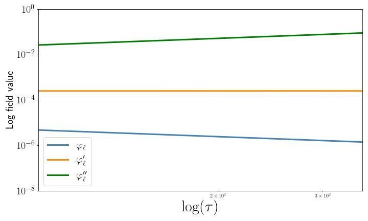
In this section, we have confirmed that our approach conserves the Aretakis charge on the horizon and can correctly reproduce the related instability [2, 3] for axisymmetric and non-axisymmetric perturbations of extremal Kerr spacetime. Our results in Fig. 7 show that the $\ell=0$ mode of the field decays as $\varphi_{\ell}(\tau,\sigma_{+})\sim\tau^{-1}$ with time $\tau$, the first spatial derivative $\partial_{\sigma}\varphi_{\ell}(\tau,\sigma)|_{\sigma=\sigma_{+}}$ (which amounts to the conserved Aretakis charge) is constant in time, and the second spatial derivative grows as $\partial_{\sigma}^{2}\varphi_{\ell}(\tau,\sigma)|_{\sigma=\sigma_{+}}\sim\tau$, in accordance with Aretakis’ theorem.

To compute the results in Fig. 7 we used a similar set up to that used for computing the late-time tails outlined in the previous section. The main differences between the two setups is that we are computing the Aretakis instability for extremal Kerr, so the spin parameter is set to $\chi=\frac{1}{2}$, that is $|a|=M$. Additionally, the initial data of the field used for the Aretakis instability was a constant function, as shown in Fig. 6. Aside from these differences, the setup used for the Aretakis instability is the same as for Price tails.

For the extremal Kerr case, Fig. 8 shows that late-time tails for axisymmetric modes $(l,m,s)$ $=(0,0,0)$ and $(0,1,0)$ decay as $\varphi_{\ell}(\tau,\sigma_{+})\sim\tau^{-2\ell-1}$ and that the Aretakis charge e $(\varphi_{\ell})^{\prime}=\partial_{\sigma}\varphi_{\ell}(\tau,\sigma)|_{\sigma=\sigma_{+}}$ is conserved on the future horizon $\mathcal{H^{+}}$, in accordance with Aretakis’ theorem. In the non-axisymmetric case, superradiance leads to an enhanced growth rate of the Aretakis instability. Fig. 8 shows that tails for non-axisymmetric modes $(l,m,s)=$ $(0,2,0)$ and $(1,2,0)$ decay as $\varphi_{\ell}(\tau,\sigma_{+})\sim\tau^{-1/2}$ on the horizon. Fig. 9 shows that the Aretakis charge $(\varphi^{2}_{\ell})^{\prime}=\partial_{\sigma}\varphi^{2}_{\ell}(\tau,\sigma)|_{\sigma=\sigma_{+}}$ for a non-axisymmetric mode $(l,m,s)=$ $(2,2,0)$ is conserved on $\mathcal{H^{+}}$. This is in accordance with predictions made by Casals, Gralla and Zimmerman [17, 9, 18] using Laplace transform techniques.

Figure 7: Decay for solutions of the wave equation on extremal Kerr spacetimes $|a|=M$, for the fundamental axisymmetric mode $(l,m,s)=(0,0,0)$, exhibiting the Aretakis instability. The left plot shows that the field on the horizon decreases with time as $\varphi_{\ell}(\tau,\sigma_{+})\sim\tau^{-1}$, the first spatial derivative of the field is constant in time, $\varphi^{\prime}_{\ell}=\partial_{\sigma}\varphi_{\ell}(\tau,\sigma)|_{\sigma=\sigma_{+}}\sim\tau^{0}$, and the second spatial derivative of the field increases with time as $\varphi^{\prime\prime}_{\ell}=\partial_{\sigma}^{2}\varphi_{0}(\tau,\sigma)|_{\sigma=\sigma_{+}}\sim\tau$. The results were calculated using a pseudo-spectral grid of 96 points. The right plot shows the error in the conserved first derivative of the field.

Figure 8: Late-time tails for the extremal Kerr case for spin $s=0$ fields. The left plot for axisymmetric mode $m=0$ shows that the field decays as $\varphi_{\ell}(\tau,\sigma_{+})\sim\tau^{\ell-2l-1}$ on the horizon, in accordance with Aretakis’ theorem. The right plot for non-axisymmetric mode $m=2$ shows that the field decays as $\varphi_{\ell}(\tau,\sigma_{+})\sim\tau^{-1/2}$, in accordance with predictions made by Casals, Gralla and Zimmerman [17, 9, 18].

Figure 9: Consevation of a non-axisymmetric Aretakis charge for solutions of the wave equation on extremal Kerr spacetimes $|a|=M$. The plot shows the error in the real and imaginary part of the charge $(\varphi^{2}_{\ell})^{\prime}=\partial_{\sigma}\varphi^{2}_{\ell}(\tau,\sigma)|_{\sigma=\sigma_{+}}\sim\tau^{0}$ for a non-axisymmetric mode $(l,m,s)=(2,2,0)$, which is conserved on the future horizon $\mathscr{H}^{+}$ as predicted by Gralla et al. [17, 9, 18]. The results were calculated using a pseudo-spectral grid of 96 points.

References

- [1] Y. Angelopoulos, S. Aretakis, and D. Gajic. Late-time tails and mode coupling of linear waves on Kerr spacetimes. arXiv:2102.11884 [gr-qc], Feb. 2021.
- [2] S. Aretakis. Horizon Instability of Extremal Black Holes, Mar. 2013.
- [3] S. Aretakis. Dynamics of Extremal Black Holes, volume 33 of SpringerBriefs in Mathematical Physics. Springer International Publishing, Cham, 2018.
- [4] L. Barack. Late time decay of scalar, electromagnetic, and gravitational perturbations outside rotating black holes. Physical Review D, 61(2):024026, Dec. 1999.
- [5] L. Barack and P. Giudice. Time-domain metric reconstruction for self-force applications. Physical Review D, 95(10):104033, May 2017.
- [6] J. M. Bardeen and W. H. Press. Radiation fields in the Schwarzschild background. Journal of Mathematical Physics, 14(1):7–19, 1973.
- [7] D. Bini, C. Cherubini, R. T. Jantzen, and R. J. Ruffini. Teukolsky Master Equation: De Rham wave equation for the gravitational and electromagnetic fields in vacuum. Progress of Theoretical Physics, 107(5):967–992, May 2002.
- [8] C. Canuto, M. Hussaini, A. Quarteroni, and T. Zang. Spectral methods. Jan. 2006.
- [9] M. Casals, S. E. Gralla, and P. Zimmerman. Horizon Instability of Extremal Kerr Black Holes: Nonaxisymmetric Modes and Enhanced Growth Rate. Physical Review D, 94(6):064003, Sept. 2016.
- [10] R. Courant, K. Friedrichs, and H. Lewy. On the Partial Difference Equations of Mathematical Physics. IBM Journal of Research and Development, 11(2):215–234, Mar. 1967.
- [11] K. Csukás, I. Rácz, and G. Z. Tóth. Numerical investigation of the dynamics of linear spin s fields on Kerr background I. Late time tails of spin $s = \pm 1, \pm 2$ fields. Physical Review D, 100(10):104025, Nov. 2019.
- [12] M. Dafermos, I. Rodnianski, and Y. Shlapentokh-Rothman. Decay for solutions of the wave equation on Kerr exterior spacetimes III: The full subextremal case |a| M. 2016, 183(3):787–913, Dec. 2014.
- [13] N. Deppe, L. E. Kidder, M. A. Scheel, and S. A. Teukolsky. Critical behavior in 3-d gravitational collapse of massless scalar fields. Physical Review D, 99(2):024018, Jan. 2019.
- [14] S. R. Dolan. Superradiant instabilities of rotating black holes in the time domain. Physical Review D, 87(12), June 2013.
- [15] S. E. Field, S. Gottlieb, Z. J. Grant, L. F. Isherwood, and G. Khanna. A GPU-Accelerated Mixed-Precision WENO Method for Extremal Black Hole and Gravitational Wave Physics Computations. Communications on Applied Mathematics and Computation, May 2021.
- [16] J. N. Goldberg, A. J. Macfarlane, E. T. Newman, F. Rohrlich, and E. C. G. Sudarshan. Spin-s Spherical Harmonics and ð. Journal of Mathematical Physics, 8(11):2155–2161, Nov. 1967.
- [17] S. E. Gralla, A. Zimmerman, and P. Zimmerman. Transient Instability of Rapidly Rotating Black Holes. Physical Review D, 94(8):084017, Oct. 2016.
- [18] S. E. Gralla and P. Zimmerman. Critical Exponents of Extremal Kerr Perturbations. Classical and Quantum Gravity, 35(9):095002, May 2018.
- [19] E. Harms, S. Bernuzzi, and B. Bruegmann. Numerical solution of the 2+1 Teukolsky equation on a hyperboloidal and horizon penetrating foliation of Kerr and application to late-time decays. Classical and Quantum Gravity, 30(11):115013, June 2013.
- [20] E. Harms, S. Bernuzzi, A. Nagar, and A. Zenginoğlu. A new gravitational wave generation algorithm for particle perturbations of the Kerr spacetime. Classical and Quantum Gravity, 31(24):245004, Nov. 2014.
- [21] D. Hilditch. An Introduction to Well-posedness and Free-evolution. International Journal of Modern Physics A, 28(22n23):1340015, Sept. 2013.
- [22] M. Hochbruck and A. Ostermann. Exponential integrators. Acta Numerica, 19:209–286, May 2010.
- [23] J. L. Jaramillo, R. P. Macedo, and L. A. Sheikh. Pseudospectrum and black hole quasi-normal mode (in)stability. arXiv:2004.06434 [gr-qc, physics:hep-th, physics:math-ph], Jan. 2021.
- [24] T. S. Keidl, A. G. Shah, J. L. Friedman, D.-H. Kim, and L. R. Price. Gravitational Self-force in a Radiation Gauge. Physical Review D, 82(12):124012, Dec. 2010.
- [25] R. P. Kerr. Gravitational Field of a Spinning Mass as an Example of Algebraically Special Metrics. Physical Review Letters, 11(5):237–238, Sept. 1963.
- [26] H.-O. Kreiss and G. Scherer. Method of Lines for Hyperbolic Differential Equations. SIAM Journal on Numerical Analysis, 29(3):640–646, 1992.
- [27] J. M. Landsberg. Tensors: Geometry and Applications. Number 128 in Graduate Studies in Mathematics. 2012.
- [28] O. Long and L. Barack. Time-domain metric reconstruction for hyperbolic scattering. Physical Review D, 104(2):024014, July 2021.
- [29] J. Lucietti and H. S. Reall. Gravitational instability of an extreme Kerr black hole. Physical Review D: Particles and Fields, 86(10):104030, Nov. 2012.
- [30] R. P. Macedo. Hyperboloidal framework for the Kerr spacetime. Classical and Quantum Gravity, 37(6):065019, Mar. 2020.
- [31] R. P. Macedo and M. Ansorg. Axisymmetric fully spectral code for hyperbolic equations. Journal of Computational Physics, 276:357–379, Nov. 2014.
- [32] C. Markakis, M. F. O’Boyle, P. D. Brubeck, and L. Barack. Discontinuous collocation methods and gravitational self-force applications. Classical and Quantum Gravity, 38(7):075031, Apr. 2021.
- [33] C. M. Markakis, M. F. O’Boyle, D. Glennon, K. Tran, P. Brubeck, R. Haas, H.-Y. Schive, and K. Uryū. Time-symmetry, symplecticity and stability of Euler-Maclaurin and Lanczos-Dyche integration. arXiv:1901.09967 [math-ph, physics:physics], Jan. 2019.
- [34] C. Merlin, A. Ori, L. Barack, A. Pound, and M. van de Meent. Completion of metric reconstruction for a particle orbiting a Kerr black hole. Physical Review D, 94(10):104066, Nov. 2016.
- [35] E. Newman and R. Penrose. An Approach to Gravitational Radiation by a Method of Spin Coefficients. Journal of Mathematical Physics, 3(3):566–578, May 1962.
- [36] M. F. O’Boyle, C. Markakis, L. J. G. Da Silva, R. P. Macedo, and J. A. V. Kroon. Conservative Evolution of Black Hole Perturbations with Time-Symmetric Numerical Methods, Oct. 2022.
- [37] P. Papadopoulos and J. A. Font. Relativistic hydrodynamics on spacelike and null surfaces: Formalism and computations of spherically symmetric spacetimes. Physical Review D, 61(2):024015, Dec. 1999.
- [38] A. Pound, C. Merlin, and L. Barack. Gravitational self-force from radiation-gauge metric perturbations. Physical Review D, 89(2):024009, Jan. 2014.
- [39] W. H. Press and S. A. Teukolsky. Perturbations of a Rotating Black Hole. II. Dynamical Stability of the Kerr Metric. The Astrophysical Journal, 185:649, Oct. 1973.
- [40] R. H. Price. Nonspherical Perturbations of Relativistic Gravitational Collapse. I. Scalar and Gravitational Perturbations. Physical Review D, 5(10):2419–2438, May 1972.
- [41] R. H. Price. Nonspherical Perturbations of Relativistic Gravitational Collapse. II. Integer-Spin, Zero-Rest-Mass Fields. Physical Review D, 5(10):2439–2454, May 1972.
- [42] I. Racz and G. Z. Toth. Numerical investigation of the late-time Kerr tails. Classical and Quantum Gravity, 28(19):195003, Oct. 2011.
- [43] J. L. Ripley. Computing the quasinormal modes and eigenfunctions for the Teukolsky equation using horizon penetrating, hyperboloidally compactified coordinates. Classical and Quantum Gravity, 39(14):145009, July 2022.
- [44] D. Schinkel, M. Ansorg, and R. P. Macedo. Initial data for perturbed Kerr black holes on hyperboloidal slices. Classical and Quantum Gravity, 31(16):165001, Aug. 2014.
- [45] D. Schinkel, R. Panosso Macedo, and M. Ansorg. Axisymmetric constant mean curvature slices in the Kerr space-time. 31:075017, 2014.
- [46] A. Shah, T. Keidl, J. Friedman, D.-H. Kim, and L. Price. Conservative, gravitational self-force for a particle in circular orbit around a Schwarzschild black hole in a Radiation Gauge. Physical Review D, 83(6):064018, Mar. 2011.
- [47] A. G. Shah, J. L. Friedman, and B. F. Whiting. Finding high-order analytic post-Newtonian parameters from a high-precision numerical self-force calculation. Physical Review D, 89(6):064042, Mar. 2014.
- [48] S. A. Teukolsky. Perturbations of a Rotating Black Hole. I. Fundamental Equations for Gravitational, Electromagnetic, and Neutrino-Field Perturbations. The Astrophysical Journal, 185:635, Oct. 1973.
- [49] S. A. Teukolsky and W. H. Press. Perturbations of a rotating black hole. III - Interaction of the hole with gravitational and electromagnetic radiation. The Astrophysical Journal, 193:443, Oct. 1974.
- [50] G. Z. Toth. Noether currents for the Teukolsky Master Equation. Class. Quantum Grav., 35(18):185009, Sept. 2018.
- [51] S. D. Upton and A. Pound. Second-order gravitational self-force in a highly regular gauge. Physical Review D, 103(12):124016, June 2021.
- [52] I. Vega, B. Wardell, and P. Diener. Effective source approach to self-force calculations. Classical and Quantum Gravity, 28(13):134010, June 2011.
- [53] A. Zenginoglu. A Hyperboloidal study of tail decay rates for scalar and Yang-Mills fields. 25(AEI-2008-015):175013, 2008.
- [54] A. Zenginoğlu. A hyperboloidal study of tail decay rates for scalar and Yang-Mills fields. Classical and Quantum Gravity, 25(17):175013, Sept. 2008.
- [55] A. Zenginoğlu, G. Khanna, and L. M. Burko. Intermediate behavior of Kerr tails. General Relativity and Gravitation, 46(3):1672, Mar. 2014.
- [56] A. Zenginoglu and M. Tiglio. Spacelike matching to null infinity. Physical Review D, 80(2):024044, July 2009.