Coupling Enhancement and Symmetrization in Dissipative Optomechanical Systems

Abstract

Observing few-photon optomechanical effects remains a significant challenge in optomechanical systems. To investigate intrinsic radiation-pressure-induced nonlinear effects in the few-photon regime, it is essential to strengthen the interaction between few photons and a finite number of phonons. In this work, we enhance the radiation-pressure nonlinearity by introducing a two-laser coherent driving scheme together with an enhanced cross-Kerr nonlinearity, resulting in a setup that can be effectively described within a circuit QED platform. By properly tuning the two driving laser fields and the cross-Kerr interaction so that the effective optomechanical coupling becomes real, we theoretically establish a symmetric optomechanical model in which the photon and phonon modes exhibit analogous fluctuation dynamics. Within this framework, we analyze the optimal reciprocal transport of the input laser field and identify the critical boundary associated with the onset of different coupling regimes. We also compare the optical signal scattering behavior in both dissipative equilibrium and nonequilibrium symmetric optomechanical systems, with and without non-rotating-wave contributions. Our work provides a controllable route to enhance optomechanical coupling, extending into the ultrastrong-coupling regime, and opens opportunities for exploring few-photon optomechanical effects.

I Introduction

Cavity optomechanics is a rapidly developing research field involving quantum optics and nanoscience ref-1 ; ref-2 ; ref-3 . Work in this field focuses on studying the radiation-pressure (RP) coupling between electromagnetic and mechanical degrees of freedom ref-4 ; ref-5 ; ref-6 . Recently, particular interest has been devoted to exploring optomechanical effects in the few-photon regime ref-7 ; ref-8 ; ref-9 , as exploiting the intrinsic nonlinear RP interaction (note that, as the dominant contribution to optomechanical nonlinearity, it is commonly referred to as the optomechanical coupling) of the cavity optomechanics would open the doors to a much vaster realm of possibilities in the quantum regime. Many unusual phenomena appear in this regime, such as the appearance of phonon sidebands in the cavity emission spectrum ref-10 , the photon blockade effect due to a weakly driving laser ref-11 ; ref-12 ; ref-13 ; ref-14 , and the generation of macroscopic quantum superposition ref-15 ; ref-16 .

However, optomechanical effects in the few-photon regime, especially at the single-photon level, have not yet been observed under existing experimental techniques ref-2 . This difficulty arises because the radiation-pressure coupling involving only a few photons is typically too weak to be resolved from environmental noise in the standard optomechanical systems ref-17 . Consequently, enhancing the optomechanical coupling to reach the strong- or even ultrastrong-coupling regime in cavity optomechanics involving few photons remains a nontrivial task. To date, many schemes have been proposed to enhance the optomechanical coupling in the few-photon regime. These schemes include the generation of collective density excitation of the Bose-Einstein condensate ref-18 , the construction of an array of mechanical resonators ref-19 , the usage of the squeezing cavity mode ref-20 ; ref-21 , the exploitation of mechanical amplification ref-22 , the application of delayed quantum feedback ref-23 , and the utilization of the critical property of the lower-branch polariton cavity coupling ref-24 . In addition, recently, an all-optical system based on a Fredkin-type interaction has been proposed to simulate the ultrastrong optomechanical coupling ref-25 . Yet, there are two common issues in these schemes ref-26 . One is how to guarantee that the system operates in the few-photon regime. The other is how to ensure that radiation-pressure-induced nonlinear effects can be observed in an optomechanical system if additional sources of nonlinearity are introduced.

Motivated to resolve these issues, in this paper, we focus on a novel strategy to enhance the nonlinear effects, enabling access to the strong and even ultrastrong coupling regime with few photons in a circuit quantum electrodynamics (QED) platform. First, we propose a method to achieve controllable enhancement of the optomechanical coupling in the few-photon regime, which can be simulated on a circuit QED platform. In contrast to the hybrid cavity optomechanics or optomechanical-like systems, we stress that our scheme is realized by considering only two points. One contribution stems from the enhanced second-order nonlinearity of the cavity resonance frequency beyond the radiation-pressure interaction, known as the cross-Kerr (CK) interaction ref-27 ; ref-28 , which is an inherent nonlinear interaction accompanying optomechanical coupling ref-29 ; ref-30 ; ref-31 . The other is to make sure that the mechanical resonator and the optical cavity are coherently driven by an appropriate high-power laser ref-32 ; ref-33 and a low-power one ref-34 , respectively. Second, by adjusting the parameters of the two driving lasers and the CK interaction so that the effective optomechanical coupling may become a real number, we theoretically propose effective symmetric optomechanical dynamics in the few-photon regime, in which the quantum fluctuation dynamics of the photon and phonon modes exhibit analogous forms. Third, we control the optomechanical coupling strength involving a few photons and a finite number of phonons via dual coherent laser driving and the enhanced cross-Kerr nonlinearity, achieving sequential transitions from the weak-coupling to the ultrastrong-coupling regime ref-35 ; ref-36 . By observing the critical behavior of the optimal transmission of the laser field, we identify the boundary point of the optomechanical strong coupling. In addition, we study the optimal reciprocal transport in symmetric optomechanical dynamics ref-37 ; ref-38 ; ref-39 . We also compare the scattering behavior of the laser field when the decay rate of the cavity field matches the damping rate of the mechanical oscillator or not before and after the rotating-wave approximation (RWA).

The remainder of this paper is organized as follows. In Sec. II, we introduce the physical model and derive the dynamical equations governing the system. In Sec. III, an effective symmetric optomechanical Hamiltonian is developed in the few-photon regime, and the corresponding optical and mechanical driving powers are estimated. In Sec. IV, we analyze the transmission behavior of the laser field in the symmetric optomechanical system, both with and without the rotating-wave approximation. Finally, in Sec. V, we present our conclusions and outlook.

II Coupling control of optomechanical systems

II.1 Derivation of controllable coupling setup

Figure 1: $\left(\rm{a}\right)$ A flowchart for obtaining an enhanced Hamiltonian ${H_{\rm{T}}}$. Initially, we consider an original (i.e., at single-photon level) optomechanical Hamiltonian, denoted by ${H_{\rm{O}}}$. The first step is to introduce two laser beams ${H_{\rm{d}}}\left(t\right)$ to drive the initial system. Next, we extend the above closed system $H_{\rm{S}}^{\rm{O}}$ to an open quantum system $H_{\rm{T}}^{\rm{O}}$ by adding an environmental Hamiltonian $H_{\rm{B}}^{\rm{O}}$. Then, we perform a steady-state coherent displacement transformation on it. As the last step, we safely neglect the originally enhanced CK interaction term to obtain an enhanced optomechanical Hamiltonian ${H_{\rm{T}}}$ in the few-photon regime. $\left(\rm{b}\right)$ Schematic illustration of an open optomechanical setup $H_{\rm{T}}^{\rm{O}}$ [left side of $\left(\rm{a}\right)$], which is composed of a single-mode optical field $a$ (lower side) and a mechanical mode $b$ (upper side). The optical mode is coupled to the mechanical mode via both the radiation-pressure (RP) interaction ${g_{\rm{0}}}$ $\left(\leftrightarrow\right)$ and the enhanced CK interaction $\chi$ $\left(\sim\right)$. The optical mode is coherently driven by a low-power laser $\Omega_{a}$, thereby operating in the few-photon regime, while the mechanical mode is coherently driven by a high-power laser $\Omega_{b}$, leading to the excitation of a finite number of phonons. As a result of the dual coherent laser driving, the single-photon optomechanical coupling $g_{0}$ is enhanced to an effective optomechanical coupling $g_{s}$ in the few-photon regime. Additionally, the near-resonant condition between the system modes and the corresponding reservoir modes is also considered in this open quantum system.

Figure 2: The CK enhanced setup based on a circuit quantum electrodynamics platform, which provides an effective description of the enhanced optomechanical coupling. This setup is made of superconducting qubits (orange) coupled to an on-chip cavity (green) and a nano-mechanical resonator (blue).

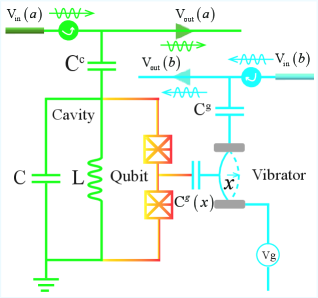
For the standard optomechanical setup, the strength of the single-photon radiation-pressure (RP) nonlinear interaction (RP nonlinearity as the dominant optomechanical nonlinearity, it is commonly referred to as the optomechanical coupling) ${g_{\rm{0}}}$ is far less than the decay rate of the optical cavity ${\kappa_{a}}$. Figure 1(a) presents the procedure for driving an optomechanical system, effectively described by a circuit quantum electrodynamics (QED), into the ultrastrong coupling regime characterized by the coupling strength $g_{\rm{s}}$ through laser control in an open quantum system. Here, ultrastrong coupling denotes the regime in which the enhanced optomechanical interaction $g_{\rm{s}}$ becomes a considerable fraction of the detuning of the mechanical resonance frequency ${{\Delta_{\rm{m}}}}$ ref-40 .

We first initialize the system by introducing a standard optomechanical Hamiltonian describing a single-mode optical cavity field coupled to a single-mode mechanical oscillator [see Fig. 1(b)]. In particular, we consider the lowest-order correction to the optomechanical interaction beyond the radiation-pressure (RP) term and neglect the rapidly oscillating terms, $\hbar\chi{a^{\dagger}}a{b^{\dagger}}{b^{\dagger}}$ and $\hbar\chi{a^{\dagger}}abb$, see Appendix A for details ref-41 ; ref-42 ; ref-43 ; ref-44 ; ref-79 ; ref-80 . Then, the Hamiltonian of the standard optomechanical model reads

$$H_{\rm{O}}=\hbar{\omega_{\rm{c}}}{a^{\dagger}}a\!+\!\hbar{\omega_{\rm{m}}}{b^{\dagger}}b\!-\!\hbar{g_{\rm{0}}}{a^{\dagger}}a\left({{b^{\dagger}}+b}\right){\rm{\!+}}\hbar\chi^{\prime}{a^{\dagger}}a{b^{\dagger}}b,$$ (1)

where ${a^{\dagger}}$ $\left(a\right)$ and ${b^{\dagger}}$ $\left(b\right)$ are the creation (annihilation) operators of the optical mode and the mechanical mode with the corresponding resonance frequencies ${\omega_{\rm{c}}}$ and ${\omega_{\rm{m}}}$, respectively. Here, the first and second terms in Eq. (1) represent the free parts of the optical and mechanical modes, respectively. The third term in Eq. (1) describes the original RP coupling between the two modes, where $g_{0}$ denotes the optomechanical coupling strength at the single-photon level, quantifying the interaction between a single photon and a single phonon. The fourth quadratic term in Eq. (1) represents the original CK interaction between the two modes, with coupling strength ${\chi^{\prime}}$.

Although the RP coupling is typically the leading interaction in optomechanical systems, the second-order nonlinear term can be substantially enhanced via Josephson junctions ref-45 or superconducting qubits ref-46 in optical implementations, a fact that has been experimentally verified ref-88 ; ref-89 ; ref-90 ; ref-91 . In our study, we focus on a CK-enhanced setup in which the CK nonlinear interaction becomes much stronger than the original RP nonlinearity ref-47 ; ref-48 ; ref-49 . Under this experimentally accessible setting within a circuit QED platform as shown in Fig. 2, the third term in Eq. (1) becomes negligible compared to the enhanced CK term, allowing us to safely adopt the approximate Hamiltonian $H_{{\rm{O}}}^{{\rm{app}}}=\hbar{\omega_{\rm{c}}}{a^{\dagger}}a+\hbar{\omega_{\rm{m}}}{b^{\dagger}}b+\hbar\chi{a^{\dagger}}a{b^{\dagger}}b$. This Hamiltonian conserves the photon number due to the commutation relation $[{{a^{\dagger}}a,H_{\rm{{O}}}}]=0$ ref-Lu053703 . In the following, based on the CK-enhanced circuit QED setup that effectively describes the enhanced optomechanical Hamiltonian ref-50 ; ref-52 , we present four steps to obtain a controllable optomechanical coupling model.

The first step. In order to enhance the optomechanical coupling, we introduce dual-laser coherent driving to the system described by the approximate Hamiltonian $H_{{\rm{O}}}^{{\rm{app}}}$. The driving Hamiltonian is given by

$${H_{\rm{d}}}\left(t\right)=\hbar\left({\Omega_{a}^{*}a{e^{i{\omega_{{L_{a}}}}t}}+\Omega_{b}^{*}b{e^{i{\omega_{{L_{b}}}}t}}}\right)+{\rm{H.c.}},$$ (2)

where the optical mode is coherently driven by a weak monochromatic field (thereby operating in the few-photon regime) with ${{\omega_{{L_{a}}}}}$ and ${\Omega_{a}}$ being the driving frequency and complex amplitude, respectively. The mechanical mode, on the other hand, is coherently driven by a strong monochromatic field (leading to the excitation of a finite number of phonons), where ${{\omega_{{L_{b}}}}}$ and ${\Omega_{b}}$ are the driving frequency and complex amplitude, respectively. The total Hamiltonian of the closed system is now given by $H_{\rm{S}}^{\rm{O}}\left(t\right)=H_{{\rm{O}}}^{{\rm{app}}}+{H_{\rm{d}}}\left(t\right)$. To make the Hamiltonian independent of time, we then move to the rotating frame of the frequency, which makes the Hamiltonian of the closed system as follows:

$${H_{\rm{S}}^{\rm{O}}} = +U\left(t\right)H_{\rm{S}}^{\rm{O}}\left(t\right){U^{\dagger}}\left(t\right)-iU\left(t\right){{\dot{U}}^{\dagger}}\left(t\right)$$ (3)

$$= +\hbar{\Delta_{\rm{c}}}{a^{\dagger}}a+\hbar{\Delta_{\rm{m}}}{b^{\dagger}}b{\rm{+}}\hbar\chi{a^{\dagger}}a{b^{\dagger}}b$$

$$+\hbar\left({\Omega_{a}^{*}a+\Omega_{b}^{*}b+{\rm{H.c.}}}\right),$$

where we used the unitary transformation of the form $U\left(t\right)=\exp[{i({{\omega_{{L_{a}}}}{a^{\dagger}}a+{\omega_{{L_{b}}}}{b^{\dagger}}b})t}]$. The parameter ${\Delta_{\rm{c}}}={\omega_{\rm{c}}}-{\omega_{{L_{a}}}}$ is the detuning of the resonant frequency ${\omega_{\rm{c}}}$ of the optical cavity $a$ from the driving frequency ${{\omega_{{L_{a}}}}}$, while ${\Delta_{\rm{m}}}={\omega_{\rm{m}}}-{\omega_{{L_{b}}}}$ is the detuning of ${\omega_{\rm{m}}}$ of the mechanical oscillator $b$ from the driving frequency ${{\omega_{{L_{b}}}}}$.

The second step. In order to extend the system to an open quantum one, we further add a system-reservoir interaction using a quantum operator approach ref-53 . The total Hamiltonian of this field-reservoir system is now written as $H_{\rm{T}}^{\rm{O}}=H_{\rm{S}}^{\rm{O}}+H_{\rm{B}}^{\rm{O}}$ with

$$H_{\rm{B}}^{\rm{O}}\!\! =\!\! +\sum\limits_{\rm{k}}{\hbar\left[{{\omega_{a{\rm{k}}}}\Gamma_{a{\rm{k}}}^{\dagger}{\Gamma_{a{\rm{k}}}}+{g_{a{\rm{k}}}}\left({{a^{\dagger}}{\Gamma_{a{\rm{k}}}}+a\Gamma_{a{\rm{k}}}^{\dagger}}\right)}\right]}$$ (4)

$$+\!\sum\limits_{\rm{k}}{\hbar\left[{{\omega_{b{\rm{k}}}}\Gamma_{b{\rm{k}}}^{\dagger}{\Gamma_{b{\rm{k}}}}+{g_{b{\rm{k}}}}\left({{b^{\dagger}}{\Gamma_{b{\rm{k}}}}+b\Gamma_{b{\rm{k}}}^{\dagger}}\right)}\right]},$$

where ${\Gamma_{a{\rm{k}}}^{\dagger}}$ $\left({{\Gamma_{a{\rm{k}}}}}\right)$ and ${\Gamma_{b{\rm{k}}}^{\dagger}}$ $\left({{\Gamma_{b{\rm{k}}}}}\right)$ are, respectively, the creation (annihilation) operators of the reservoirs for the optical mode and the mechanical mode. The present reservoir consists of many harmonic oscillators with closely spaced frequencies ${{\omega_{a{\rm{k}}}}}$ $\left({{\omega_{b{\rm{k}}}}}\right)$. The ${{g_{a{\rm{k}}}}}$ and ${{g_{b{\rm{k}}}}}$ terms represent the corresponding system-reservoir interactions.

The third step. To achieve steady-state optomechanical coupling enhancement in an open optomechanical system, we modulate the detuning of the resonant frequency of the optical cavity ${\Delta_{c}}$ by driving the mechanical oscillator $b$ (the movable mirror) with appropriate high-power laser ${{\Omega_{b}}}$, thereby enhancing the optomechanical coupling into the ultrastrong-coupling regime; that is, when the mechanical oscillator is coherently driven by a specific intense monochromatic laser ${\Omega_{b}}$ that satisfies $\left|{{\Omega_{b}}}\right|\gg\left|{{\Omega_{a}}}\right|$, the excitation number in the mechanical mode $b$ is large, and then $b$ contains a steady-state coherent part $\beta_{s}$. In other words, we employ the coherent-displacement transformation ref-54 ; ref-55 of the mechanical mode of the form $D\left(\beta\right)b{D^{\dagger}}\left(\beta\right)=b-\beta$ and ${D\left(\beta\right){b^{\dagger}}{D^{\dagger}}\left(\beta\right)=b^{\dagger}-{\beta^{*}}}$, where the unitary displacement operator is given by ${D_{b}}\left(\beta\right)=\exp\left({\beta{b^{\dagger}}-{\beta^{*}}b}\right)$ in the coherent-state representation. Since our purpose here is to obtain an optomechanical coupling enhancement at a steady state, in the following, we focus on the steady-state displacement solution ${\beta_{s}}$; we assume that the timescale of the system approaching its steady state is much shorter than other evolution timescales ref-56 . The specific form of ${\beta_{s}}$ will be given by the dynamics equation later. The total Hamiltonian $H_{\rm{T}}^{\rm{O}}$ after the transformation can be written as $H_{\rm{T}}^{{\rm{tra}}}=H_{\rm{S}}+{H_{\rm{B}}}$ with

$$H_{\rm{S}} = \!\hbar\Delta_{\rm{c}}^{0}{a^{\dagger}}a\!+\!\hbar\left({{\Delta_{\rm{m}}}\!+\!\chi{a^{\dagger}}a}\right){b^{\dagger}}b\!-\!\hbar\chi{a^{\dagger}}a\left({{\beta_{\rm{s}}}{b^{\dagger}}\!+\!\beta_{\rm{s}}^{*}b}\right)$$ (5)

$$+\hbar\left({\Omega_{a}^{*}a+\Omega_{b}^{*}b-\beta_{\rm{s}}^{*}{\Delta_{\rm{m}}}b+{\rm{H}}.{\rm{c}}.}\right)$$

$$+\hbar\Delta_{\rm{m}}\beta_{\rm{s}}^{*}{\beta_{\rm{s}}}-\hbar\Omega_{b}^{*}{\beta_{\rm{s}}}-\hbar{\Omega_{b}}\beta_{\rm{s}}^{*},$$

$${H_{\rm{B}}} = H_{\rm{B}}^{\rm{O}}-\hbar\sum\limits_{\rm{k}}{{g_{b{\rm{k}}}}}\left({\beta_{\rm{s}}^{*}{\Gamma_{b{\rm{k}}}}+{\beta_{\rm{s}}}\Gamma_{b{\rm{k}}}^{\dagger}}\right),$$ (6)

where $\Delta_{\rm{c}}^{0}={\Delta_{\rm{c}}}+\chi\beta_{\rm{s}}^{*}{\beta_{\rm{s}}}$ is the normalized optical cavity detuning including the frequency shift caused by the high-power laser coherent driving.

The fourth step. Since ${\beta_{s}}$ is controlled by the mechanical laser coherent driving, the RP optomechanical coupling can be enhanced to an effective strength $\chi{\beta_{\rm{s}}}$. After performing the coherent-displacement transformation at the steady state, the optomechanical interaction takes the form $\hbar{a^{\dagger}}a\left({{g_{s}}{b^{\dagger}}+g_{s}^{*}b}\right)$, where ${g_{\rm{s}}}=\chi{\beta_{\rm{s}}}$. Under experimentally accessible conditions in a circuit QED platform in the few-photon regime, the parameters of interest satisfy the condition $\chi{\beta_{s}}\sim{\Delta_{\rm{m}}}\gg\chi$ with ${\chi\mathord{\left/{\vphantom{\chi{{\Delta_{\rm{m}}}}}}\right.\kern-1.2pt}{{\Delta_{\rm{m}}}}}\approx{10^{-3}}$ ref-56 . Under this condition, the enhanced cross-Kerr interaction term $\chi{a^{\dagger}}a{b^{\dagger}}b$ can be negligible compared with both the mechanical detuning term ${\Delta_{\rm{m}}}{b^{\dagger}}b$ and the enhanced optomechanical interaction term $\chi{a^{\dagger}}a\left({{\beta_{s}}{b^{\dagger}}+\beta_{s}^{*}b}\right)$. Therefore, the enhanced cross-Kerr interaction term $\chi{a^{\dagger}}a{b^{\dagger}}b$ in Eq. (5) can be safely neglected ref-56 , yielding the final enhanced optomechanical Hamiltonian ${H_{\rm{T}}}$ (after shifting the origin of the energy) as follows:

$${H_{\rm{T}}} = +\hbar\Delta_{\rm{c}}^{0}{a^{\dagger}}a+\hbar{\Delta_{\rm{m}}}{b^{\dagger}}b-\hbar{a^{\dagger}}a\left({{g_{\rm{s}}}{b^{\dagger}}+g_{\rm{s}}^{*}b}\right)$$ (7)

$$+\hbar\left({\Omega_{a}^{*}a+\Omega_{b}^{*}b-\beta_{\rm{s}}^{*}{\Delta_{\rm{m}}}b+{\rm{H}}.{\rm{c}}.}\right)+{H_{\rm{B}}}.$$

Thus, the effective optomechanical coupling is enhanced from $g_{0}$, which describes the coupling between a single photon and a single phonon in Eq. (1), to $g_{s}$, corresponding to the coupling involving a few photons and a finite number of phonons in Eq. (7).

II.2 Nonlinear quantum Langevin equations

To introduce quantum damping and noise in Eq. (7) and to give the specific form of ${\beta_{s}}$, we now describe the coupling between the system and the reservoir in terms of input-output formalism ref-57 . This formalism provides us with equations of motion for the amplitude of the optical cavity field $a$ and analogously for the mechanical amplitude $b$. Substituting the final enhanced optomechanical Hamiltonian ${H_{\rm{T}}}$ into the Heisenberg equation and taking the dissipation terms with ${\kappa_{a}}$ and ${\gamma_{b}}$, as well as the corresponding noise terms with ${a_{{\rm{in}}}}$ and ${b_{{\rm{in}}}}$ into account, we find a set of closed integro-differential equations for the operators of the optical mode and mechanical mode as follows

$$\!\!\!\!\dot{a}\! = \!\!-\left[{i\Delta_{\rm{c}}^{0}+\frac{{{\kappa_{a}}}}{2}-i\left({{g_{\rm{s}}}{b^{\dagger}}+g_{\rm{s}}^{*}b}\right)}\right]a-i{\Omega_{a}}+\sqrt{{\kappa_{a}}}{a_{{\rm{in}}}},$$ (8)

$$\!\!\!\!\dot{b}\! = \!\!-\left({i{\Delta_{\rm{m}}}+\frac{{{\gamma_{b}}}}{2}}\right)b+i{g_{\rm{s}}}{a^{\dagger}}a+\sqrt{{\gamma_{b}}}{b_{{\rm{in}}}}+{{\dot{\beta}}_{\rm{s}}},$$ (9)

where ${{\kappa_{a}}}$ is the decay rate of the optical cavity field, ${{\gamma_{b}}}$ is the mechanical damping rate.

The time derivative of the steady-state displacement amplitude ${{\dot{\beta}}_{\rm{s}}}$ is equal to zero. See Appendix B for a detailed derivation of the Heisenberg-Langevin equation ref-58 ; ref-59 . From the results in Appendix B, we can see that the condition for the Heisenberg-Langevin equation to remain unchanged after the coherent displacement transformation is $\dot{\beta}\left(t\right)+\left({i{\Delta_{\rm{m}}}+0.5{\gamma_{b}}}\right)\beta\left(t\right)-i{\Omega_{b}}=0$. The solution gives the transient displacement amplitude $\beta\left(t\right)$ depending on the mechanical laser drive ${\Omega_{b}}$ in the form $\beta\left(t\right)={{{\Omega_{b}}}\mathord{\left/{\vphantom{{{\Omega_{b}}}{\left({{\Delta_{\rm{m}}}-i0.5{\gamma_{b}}}\right)}}}\right.\kern-1.2pt}{\left({{\Delta_{\rm{m}}}-i0.5{\gamma_{b}}}\right)}}+C\left({{t_{0}}}\right)\exp\left[{-\left({i{\Delta_{\rm{m}}}+0.5{\gamma_{b}}}\right)t}\right]$. In the long-time limit, the second term on the right-hand side converges to zero, and we find the steady-state coherent displacement amplitude ${\beta_{\rm{s}}}={{{\Omega_{b}}}\mathord{\left/{\vphantom{{{\Omega_{b}}}{\left({{\Delta_{\rm{m}}}-i0.5{\gamma_{b}}}\right)}}}\right.\kern-1.2pt}{\left({{\Delta_{\rm{m}}}-i0.5{\gamma_{b}}}\right)}}$. An alternative viewpoint, namely the Gorini-Kossakowski-Sudarshan-Lindblad (GKSL) master equation ref-60 ; ref-Lu180401 ; ref-Li250313731 ; ref-61 on the evaluation of the steady-state displacement amplitude ${\beta_{\rm{s}}}$ can be found in Appendix C ref-56 .

Within the Born-Markov approximation ref-62 , the incoming vacuum noise ${{a_{\rm{{in}}}}}$ of the optical cavity field in Eq. (8) and the thermal noise ${{b_{\rm{{in}}}}}$ of the mechanical oscillator in Eq. (9) are fully characterized by the following correlation functions:

$$\langle{a_{{\rm{in}}}}\rangle=0,\ \langle a_{{\rm{in}}}^{\dagger}\left(t\right){a_{{\rm{in}}}}\left({t^{\prime}}\right)\rangle=0,$$

$$\langle{a_{{\rm{in}}}}\left(t\right)a_{{\rm{in}}}^{\dagger}\left({t^{\prime}}\right)\rangle=\delta\left({t-t^{\prime}}\right),$$ (10)

$$\langle{b_{{\rm{in}}}}\rangle=0,\ \langle b_{{\rm{in}}}^{\dagger}\left(t\right){b_{{\rm{in}}}}\left({t^{\prime}}\right)\rangle={{\bar{n}}_{\rm{m}}}\delta\left({t-t^{\prime}}\right),$$

$$\langle{b_{{\rm{in}}}}\left(t\right)b_{{\rm{in}}}^{\dagger}\left({t^{\prime}}\right)\rangle=\left({{{\bar{n}}_{\rm{m}}}+1}\right)\delta\left({t-t^{\prime}}\right).$$ (11)

Here, ${{\bar{n}}_{\rm{m}}}$ is the mean thermal excitation number of the mechanical reservoir under thermal equilibrium. Equations (8) and (9) have the form of the nonlinear QLEs since both the light amplitude and the mechanical motion are driven by noise terms that comprise the vacuum noise and the thermal noise entering the system. Together with Eqs. (10) and (11), the nonlinear QLEs describe the evolution of the optical cavity field and the mechanical oscillator, including dissipations $\left({{\kappa_{a}},{\gamma_{b}}}\right)$ and incoming noises $\left({{a_{\rm{{in}}}},{b_{\rm{{in}}}}}\right)$.

To find the standard form of the nonlinear QLEs, we consider the particular case in which the steady-state displacement amplitude ${{\beta_{\rm{s}}}}$ satisfies the following condition:

$${\beta_{\rm{s}}}=\beta_{\rm{s}}^{*}=\left|{{\beta_{\rm{s}}}}\right|=\beta_{\rm{s}}^{R}>0.$$ (12)

In other words, the steady-state displacement amplitude ${\beta_{\rm{s}}}$ is real and positive, which is specifically denoted by $\beta_{\rm{s}}^{R}$. By assuming the laser amplitude ${\Omega_{b}}=i{\varepsilon_{b}}\exp\left({i{\varphi_{b}}}\right)$, where ${\varepsilon_{b}}$ denotes the laser power and ${\varphi_{b}}$ denotes the phase of the laser field coupling to the mechanical mode, we obtain the steady-state solution satisfying Eq. (12) as

$$\beta_{\rm{s}}^{R}=-\frac{{2{\varepsilon_{b}}\cos\left({{\varphi_{b}}}\right)}}{{{\gamma_{b}}}}\geq 0,\quad\tan\left({{\varphi_{b}}}\right)=\frac{{2{\Delta_{\rm{m}}}}}{{{\gamma_{b}}}}\geq 0$$ (13)

with ${\varphi_{b}}\in[{\pi,1.5\pi})$. Meeting the above conditions, we arrive at the standard nonlinear QLEs as follows:

$$\dot{a}\!\! = \!\!\!-\left({i\Delta_{\rm{c}}^{0}+\frac{{{\kappa_{a}}}}{2}}\right)a\!+\!i{g}\left({{b^{\dagger}}+b}\right)a\!+\!\sqrt{{\kappa_{a}}}{a_{\rm{in}}}\!-\!i{\Omega_{a}},$$ (14)

$$\dot{b}\!\! = \!\!\!-\left({i{\Delta_{\rm{m}}}+\frac{{{\gamma_{b}}}}{2}}\right)b+i{g}{a^{\dagger}}a+\sqrt{{\gamma_{b}}}{b_{\rm{in}}},$$ (15)

where ${g_{\rm{s}}}=g_{\rm{s}}^{*}=g=\chi\beta_{\rm{s}}^{R}$ is the controllable optomechanical coupling strength in the few-photon regime.

III Symmetrical optomechanical dynamics at single-photon level

Before presenting the dynamical analysis, we first emphasize that the construction of a symmetric optomechanical system serves as a framework and provides a baseline for analyzing multimode asymmetric optomechanical systems. Within this symmetric optomechanical framework, we show that the photon and phonon modes exhibit fluctuation dynamics of analogous forms. We then analyze the optimal reciprocal transport of the input laser field and identify the critical boundary associated with the onset of different coupling regimes. Furthermore, we compare the optical scattering behavior in dissipative equilibrium and nonequilibrium symmetric systems, both with and without non-rotating-wave contributions. Notably, we generalize the scattering-probability expression of Ref. ref-81 to a broadly applicable form that is valid not only in the weak-coupling regime but also accurately captures the strong- and ultrastrong-coupling regimes.

III.1 Real optomechanical coupling

The nonlinear QLEs. (14) and (15) are inherently nonlinear, as they contain products of photon (i.e., optical cavity mode $a$) and phonon (i.e., mechanical mode $b$) operators, ${ab}$ and ${a{b^{\dagger}}}$, as well as a quadratic term in the photon operators, $a^{\dagger}a$. To proceed, we apply the linearization procedure to Eqs. (14) and (15). To this end, we decompose the photon and phonon operators into their classical mean values [i.e., average coherent amplitudes $\langle a\rangle\approx\alpha$ ($\langle{{a^{\dagger}}}\rangle\approx{\alpha^{*}}$) and $\langle b\rangle\approx\beta$ ($\langle{{b^{\dagger}}}\rangle\approx{\beta^{*}}$)] and quantum fluctuation operators [i.e., $\delta a$ ($\delta{a^{\dagger}}$) and $\delta b$ ($\delta{b^{\dagger}}$)], namely, $a=\alpha+\delta a$ ($a^{\dagger}=\alpha^{*}+\delta a^{\dagger}$) and $b=\eta+\delta b$ ($b^{\dagger}=\eta^{*}+\delta b^{\dagger}$) ref-2 . Following this approach, the solution of the complex mean values for the classical steady state satisfies

$$\dot{\alpha} = -\left({i\Delta_{c}^{0}+\frac{{{\kappa_{a}}}}{2}}\right)\alpha+i{g}\left({{\eta^{*}}+\eta}\right)\alpha-i{\Omega_{a}},$$ (16)

$$\dot{\eta} = -\left({i{\Delta_{\rm{m}}}+\frac{{{\gamma_{b}}}}{2}}\right)\eta+i{g}{\left|\alpha\right|^{2}}.$$ (17)

By solving Eqs. (16) and (17), we obtain the solution of the complex mean values $\alpha$ and $\eta$ for the classical steady state as follows:

$$\alpha = \frac{{-i{\Omega_{a}}\left[{{{\left({\frac{{{\gamma_{b}}}}{2}}\right)}^{2}}+{{\left({{\Delta_{\rm{m}}}}\right)}^{2}}}\right]}}{{\left({i\Delta_{\rm{c}}^{0}+\frac{{{\kappa_{a}}}}{2}}\right)\left[{{{\left({\frac{{{\gamma_{b}}}}{2}}\right)}^{2}}+{{\left({{\Delta_{\rm{m}}}}\right)}^{2}}}\right]-2i{g^{2}}{\Delta_{\rm{m}}}{{\left|\alpha\right|}^{2}}}},$$

$$\eta = \frac{{ig{{\left|\alpha\right|}^{2}}}}{{i{\Delta_{\rm{m}}}+\frac{{{\gamma_{b}}}}{2}}}.$$ (18)

On the other hand, the quantum fluctuation operators $\delta a$ and $\delta b$ satisfy the following nonlinear equations of motion:

$$\delta\dot{a} = -\left({i{\Delta^{\prime}_{\rm{c}}}+\frac{{{\kappa_{a}}}}{2}}\right)\delta a+i{g}\alpha\left({\delta{b^{\dagger}}+\delta b}\right)$$ (19)

$$+i{g}\delta a\left({\delta{b^{\dagger}}+\delta b}\right)+\sqrt{{\kappa_{a}}}\delta{a_{\rm{in}}},$$

$$\delta\dot{b} = -\left({i{\Delta_{\rm{m}}}+\frac{{{\gamma_{b}}}}{2}}\right)\delta b+i{g}\left(\alpha\delta{a^{\dagger}}+{{\alpha^{*}}\delta a}\right)$$ (20)

$$+i{g}\delta{a^{\dagger}}\delta a+\sqrt{{\gamma_{b}}}\delta{b_{\rm{in}}},$$

where the detuning frequency of the optical cavity field is renormalized as ${{\Delta^{\prime}_{\rm{c}}}}=\Delta_{\rm{c}}^{0}-g\left({\eta+{\eta^{*}}}\right)$.

Since the optical mode is weakly driven by a coherent laser field, while the mechanical mode is strongly coherently driven, as shown in Fig. 3(a), a coherent background generated by dual laser driving and involving a few photons and a finite number of phonons is established (details are provided in Sec. II). Given this physical scenario, the linearized description is valid provided that the number fluctuations of the photon and phonon modes remain sufficiently small (in the ultrastrong optomechanical coupling regime under few-photon conditions, they differ by about an order of magnitude or more; see Sec. III.2 for a detailed analysis) compared to their corresponding average populations, i.e., $\langle\delta a^{\dagger}\delta a\rangle\ll\langle a^{\dagger}a\rangle\approx|\alpha|^{2}$ and $\langle\delta b^{\dagger}\delta b\rangle\ll\langle b^{\dagger}b\rangle\approx|\eta|^{2}$. Thus, the dominant contributions in Eqs. (19) and (20) arise from the first-order linear terms $i{g}\alpha\left({\delta{b^{\dagger}}+\delta b}\right)$ and $i{g}\left(\alpha\delta{a^{\dagger}}+{{\alpha^{*}}\delta a}\right)$. By neglecting the second-order nonlinear terms $ig\,\delta a(\delta b^{\dagger}+\delta b)$ and $ig\,\delta a^{\dagger}\delta a$, Eqs. (19) and (20) can be linearized, yielding the linearized QLEs for $\delta a$ and $\delta b$:

$$\!\delta\dot{a}\!\! = \!\!\!-\!\left({i{\Delta^{\prime}_{\rm{c}}}\!+\!\frac{{{\kappa_{a}}}}{2}}\right)\delta a\!+\!i{g}\alpha\left({\delta{b^{\dagger}}\!+\!\delta b}\right)\!+\!\!\sqrt{{\kappa_{a}}}\delta{a_{\rm{in}}},$$ (21)

$$\!\delta\dot{b}\!\! = \!\!\!-\!\left({i{\Delta_{\rm{m}}}\!+\!\frac{{{\gamma_{b}}}}{2}}\right)\delta b\!+\!i{g}\left(\alpha\delta{a^{\dagger}}\!+\!{{\alpha^{*}}\delta a}\right)\!+\!\!\sqrt{{\gamma_{b}}}\delta{b_{\rm{in}}},$$ (22)

which are easy to solve analytically in the frequency domain after Fourier transformation. Furthermore, by observing the form of Eqs. (21) and (22), we find that Eq. (21), which describes the dynamical evolution of the photon fluctuation operator, and Eq. (22), which depicts the dynamical behavior of the phonon fluctuation operator, are completely symmetrized when we meet the following two conditions simultaneously in this open quantum system.

The first condition is to set the average value $\alpha$ of the photons in the classical steady state to a real number ${\alpha_{R}}$. With this restriction, we can determine the real mean value of the classical steady state of the photons ${\alpha_{R}}$ and ${\eta_{{\alpha_{R}}}}$ (the value of $\eta$ for a fixed value ${\alpha_{R}}$) from Eqs. (16) and (17) as follows:

$${\varepsilon_{a}}\cos\left({{\varphi_{a}}}\right)-\frac{{{\kappa_{a}}}}{2}{\alpha_{R}} = 0,$$ (23)

$$i{g}{\left({{\alpha_{R}}}\right)^{2}}-\left({i{\Delta_{\rm{m}}}+\frac{{{\gamma_{b}}}}{2}}\right){\eta_{{\alpha_{R}}}} = 0,$$ (24)

$${\varepsilon_{a}}\sin\left({{\varphi_{a}}}\right)-{\alpha_{R}}{\Delta^{\prime\prime}_{\rm{c}}} = 0,$$ (25)

where we set the laser amplitude ${\Omega_{a}}$ to $i{\varepsilon_{a}}\exp\left({i{\varphi_{a}}}\right)$ with ${\varepsilon_{a}}$ denoting the laser power and ${{\varphi_{a}}}$ the phase of the laser field coupling to the optical mode. We also defined ${\Delta^{\prime\prime}_{\rm{c}}}=\Delta_{\rm{c}}^{0}-g\left({{\eta_{{\alpha_{R}}}}+\eta_{{\alpha_{R}}}^{*}}\right)$ as a modified detuning frequency of the optical cavity field. We transform Eqs. (23)-(25) as follows:

$${\alpha_{R}} = \frac{{2{\varepsilon_{a}}\cos\left({{\varphi_{a}}}\right)}}{{{\kappa_{a}}}},\ \ {\eta_{{\alpha_{R}}}}=\frac{{2ig{\left({{\alpha_{R}}}\right)^{2}}}}{{2i{\Delta_{\rm{m}}}+{\gamma_{b}}}},$$ (26)

$$\tan\left({{\varphi_{a}}}\right) = \frac{{2{\Delta^{\prime\prime}_{\rm{c}}}}}{{{\kappa_{a}}}}=\frac{2}{{{\kappa_{a}}}}\left[{\Delta_{\rm{c}}^{0}-g\left({{\eta_{{\alpha_{R}}}}+\eta_{{\alpha_{R}}}^{*}}\right)}\right].$$ (27)

Substituting Eq. (26) into Eq. (27), we obtain a nonlinear equation for ${{\varphi_{a}}}$ in the form

$$\!\!\tan\left({{\varphi_{a}}}\right)\!=\!\!\frac{2}{{{\kappa_{a}}}}\!\!\left\{{\Delta_{\rm{c}}^{0}\!\!-\!\!\frac{{8{\Delta_{\rm{m}}}}}{{4{{\left({{\Delta_{\rm{m}}}}\right)}^{2}}\!\!+\!\!{{\left({{\gamma_{b}}}\right)}^{2}}}}{{\left[{\frac{{2g{\varepsilon_{a}}\cos\left({{\varphi_{a}}}\right)}}{{{\kappa_{a}}}}}\right]}^{2}}}\right\}\!.$$ (28)

Since ${\alpha_{R}}>0$, we find the solution of Eq. (28) in the range: ${\varphi_{a}}\in\left[{0,0.5\pi}\right)\cup\left({1.5\pi,2\pi}\right]$. We note that, when $\alpha$ is taken as a complex mean value satisfying the classical steady-state solution, its phase may break the symmetry of the dynamics and induce nonreciprocal transmission in general. Although this mechanism is not operative in a two-mode case (since the physical phase angle can be eliminated by a suitable transformation of the reference frame), it can become relevant in more general multimode configurations ref-65 ; ref-Yang2505.10255 ; ref-Yi2503.23169 ; ref-Luan2503.18647 .

Now, substituting the expressions (26) into Eqs. (21) and (22), we can reduce them to the following forms:

$$\delta\dot{a}\!\! = \!\!\!-\!\left({i{{\Delta^{\prime\prime}_{\rm{c}}}}+\frac{{{\kappa_{a}}}}{2}}\right)\delta a\!+\!i{G_{R}}\left({\delta{b^{\dagger}}+\delta b}\right)\!+\!\!\sqrt{{\kappa_{a}}}\delta{a_{\rm{in}}},$$ (29)

$$\delta\dot{b}\!\! = \!\!\!-\!\left({i{\Delta_{\rm{m}}}+\frac{{{\gamma_{b}}}}{2}}\right)\delta b\!+\!i{G_{R}}\left({\delta{a^{\dagger}}+\delta a}\right)\!+\!\!\sqrt{{\gamma_{b}}}\delta{b_{\rm{in}}},$$ (30)

where ${G_{R}}={g}{\alpha_{R}}$ is an effective optomechanical coupling in the linearized regime. It is enhanced compared to ${g}$ by the real amplitude ${\alpha_{R}}$ of the photon field.

Equations (29) and (30) show the formal equivalence of the quantum fluctuation dynamics of photons and phonons. The corresponding effective Hamiltonian of the system under the Heisenberg picture (time-dependent operator) is given by ${H_{{\rm{eff}}}}=\hbar{\Delta^{\prime\prime}_{\rm{c}}}{a^{\dagger}}a+\hbar{\Delta_{\rm{m}}}{b^{\dagger}}b-\hbar{G_{R}}\left({{a^{\dagger}}+a}\right)\left({{b^{\dagger}}+b}\right)$. Hereafter, we refer to ${H_{{\rm{eff}}}}$ as the effective Hamiltonian of the symmetric optomechanical system, in which the interaction form describes a general linear coupling between two bosonic modes in quantum optics. Moreover, we know that the Hamiltonian of the Jaynes-Cummings model describing the atom-field interaction has a similar interaction form $\hbar g({a^{\dagger}}+a)({\sigma_{+}}+{\sigma_{-}})$, where the operator ${{\sigma_{+}}}$ takes an atom in the lower state into the upper state whereas ${{\sigma_{-}}}$ has the opposite effect. Thus, the effective symmetric Hamiltonian ${H_{{\rm{eff}}}}$ provides a general formalism for linear light-matter interactions in quantum optics, and the resulting conclusions are of broad applicability.

Another condition for achieving the equivalence of the quantum fluctuation dynamics of the photon and phonon modes is to set the corresponding parameters in Eqs. (29) and (30) equal to each other. To be specific, we equalize the modified detuning frequency ${{\Delta^{\prime\prime}_{c}}}$ of the optical cavity field to the detuning of the mechanical resonance frequency ${{\Delta_{\rm{m}}}}$ by adjusting the two driving lasers ${\Omega_{a}}$ and ${\Omega_{b}}$. We also equalize the decay ${{\kappa_{a}}}$ of the optical cavity field to the damping ${{\gamma_{b}}}$ of the mechanical oscillator by modulating the corresponding system-reservoir interaction ${g_{a{\rm{k}}}}$ and ${g_{b{\rm{k}}}}$. To implement this scenario, we carefully analyze and compare representative works in the theoretical proposal and experimental results concerning the optomechanical systems with the enhanced CK interaction; see Table 1. We see that circuit quantum electrodynamic systems provide a practical platform for realizing the above scenario, where the parameter conditions ${\Delta^{\prime\prime}_{\rm{c}}}={\Delta_{\rm{m}}}$ and ${\kappa_{a}}={\gamma_{b}}$ are experimentally achievable. In circuit QED, the cavity decay rate ${\kappa_{a}}$ can be tuned via the external coupling between the resonator and transmission lines, while the effective mechanical damping rate ${\gamma_{b}}$ with parametric mechanical driving can be independently engineered through dissipative coupling or reservoir engineering, allowing the condition ${\kappa_{a}}={\gamma_{b}}$ to be experimentally achieved ref-exp-1 ; ref-exp-2 . Additionally, the condition ${\Delta^{\prime\prime}_{\rm{c}}}={\Delta_{\rm{m}}}$ can be achieved experimentally by adjusting the driving fields of the optical and mechanical modes so that the resonance parameters are matched.

Table 1: Representative works in theoretical proposals and experimental results for various optomechanical systems with the CK interaction. Note that the parameters listed in the table represent typical ranges extracted from different experiments and are compatible. Typical parameters of the standard cavity optomechanical system satisfy ${\Delta^{\prime\prime}_{\rm{c}}}={\Delta_{\rm{c}}}$. The first line shows the maximum parameter values achieved by the system (5)-(6) simulated by the QED circuit after laser adjustment.

References	Type $\left({\rm{{Hz}}}\right)$	${{{{\Delta^{\prime\prime}_{\rm{c}}}}}\mathord{\left/{\vphantom{{{{\Delta^{\prime\prime}}_{\rm{c}}}}{2\pi}}}\right.\kern-1.2pt}{2\pi}}$	${{{\Delta_{\rm{m}}}}\mathord{\left/{\vphantom{{{\Delta_{\rm{m}}}}{2\pi}}}\right.\kern-1.2pt}{2\pi}}$	${{{\kappa_{a}}}\mathord{\left/{\vphantom{{{\kappa_{a}}}{2\pi}}}\right.\kern-1.2pt}{2\pi}}$	${{{\gamma_{b}}}\mathord{\left/{\vphantom{{{\gamma_{b}}}{2\pi}}}\right.\kern-1.2pt}{2\pi}}$	${\chi\mathord{\left/{\vphantom{\chi{2\pi}}}\right.\kern-1.2pt}{2\pi}}$
ref-49 ; ref-56	Circuit-QED	$5.2\times{10^{9}}$	$5.2\times{10^{9}}$	$3.3\times{10^{7}}$ ref-52	$3.3\times{10^{7}}$ ref-52	$2.5\times{10^{6}}$ ref-50
ref-66 ; ref-67	Cavity-QED	$4.8\times{10^{9}}$	$7.2\times{10^{7}}$	$4.2\times{10^{7}}$	$2.6\times{10^{6}}$	${10^{4}}\sim{10^{5}}$
ref-68 ; ref-69	Cavity-optom	$1.1\times{10^{7}}$	$7.8\times{10^{7}}$	$7.1\times{10^{6}}$	$3.4\times{10^{3}}$	$\approx 0$
ref-70 ; ref-71	Quadratic-optom	$2.8\times{10^{14}}$	$1.3\times{10^{6}}$	$5.9\times{10^{5}}$	$1.2\times{10^{-1}}$	$3.95\times{10^{-2}}$

When the two conditions mentioned above are satisfied, the quantum fluctuation dynamics of photons and phonons are completely symmetrized. Equations (29) and (30) now read

$$\delta\dot{a}\!\! = \!\!-\left({i\Delta+\frac{\xi}{2}}\right)\delta a+i{G_{R}}\left({\delta{b^{\dagger}}+\delta b}\right)\!+\!\sqrt{\xi}\delta{a_{\rm{in}}},$$ (31)

$$\delta\dot{b}\!\! = \!\!-\left({i\Delta+\frac{\xi}{2}}\right)\delta b+i{G_{R}}\left({\delta{a^{\dagger}}+\delta a}\right)\!+\!\sqrt{\xi}\delta{b_{\rm{in}}},$$ (32)

where $\Delta={\Delta^{\prime\prime}_{\rm{c}}}={\Delta_{\rm{m}}}$ and $\xi={\kappa_{a}}={\gamma_{b}}$. Equations (31) and (32) describe the quantum fluctuation dynamics of the completely symmetric optomechanics in open quantum systems. The symmetrization of the quantum fluctuation dynamics of photons and phonons reveals a more profound connection under quantum mechanics; namely, both are bosons.

III.2 Implementation of optomechanical ultrastrong coupling in the coherent-state representation

Figure 3: $\left({\rm{a}}\right)$ Schematic diagram of a symmetric optomechanical system with dual laser drives. $\left({\rm{b}}\right)$ The number of excited phonons in the system after the coherent displacement transformation at the steady state and the standard mean-field operation.

In the symmetric optomechanical Eqs. (31) and (32), as shown in Fig. 3, we adopt the form of the dual coherent laser driving in order to achieve an optomechanical ultrastrong coupling in the coherent-state representation (a detailed physical interpretation is presented in Appendix C). On the one hand, a lower-power monochromatic laser ${\Omega_{a}}$ drives the optical cavity $a$ to excite a small number of photons ${\bar{N}_{a}}$ in the optical cavity. On the other hand, a high-power monochromatic laser ${\Omega_{b}}$ drives the mechanical oscillator $b$ so that steady-state displacement amplitude ${\beta_{\rm{s}}}$ may be large enough to achieve ultrastrong optomechanical coupling. In this work, we access the ultrastrong optomechanical coupling regime with a small number of photons and a finite number of phonons by dual coherent laser driving. For practical implementation, two requirements need to be appropriately considered. First, the power of the laser field driving the optical cavity should be properly chosen such that the intracavity photon number remains small, ensuring operation in the few-photon regime. The second requirement is to determine the relationship between the laser power driving the mechanical oscillator and its steady-state displacement amplitude, in order to achieve ultrastrong optomechanical coupling.

First, we evaluate the relationship between the number of photons in the system and the low-power driving laser. We know from Eq. (26) that the average photon number acting on the symmetrical optomechanical system is given by

$${{\bar{N}}_{a}}={\alpha_{R}}^{2}=2{\left({\frac{{{\varepsilon_{a}}}}{{{\kappa_{a}}}}}\right)^{2}}\left[{\cos\left({2{\varphi_{a}}}\right)+1}\right],$$ (33)

in which ${\varepsilon_{a}}$ is related to the driving laser power ${P_{a}}$ by ${\varepsilon_{a}}=\left|{{\Omega_{a}}}\right|=\sqrt{{{2{P_{a}}{\kappa_{a}}}\mathord{\left/{\vphantom{{2{P_{a}}{\kappa_{a}}}{\hbar{\omega_{{L_{a}}}}}}}\right.\kern-1.2pt}{\hbar{\omega_{{L_{a}}}}}}}$. Equation (33) can therefore be rewritten as

$$0\leq{{\bar{N}}_{a}}=\frac{{4{P_{a}}\left[{\cos\left({2{\varphi_{a}}}\right)+1}\right]}}{{\hbar{\omega_{{L_{a}}}}{\kappa_{a}}}}\leq\frac{{8{P_{a}}}}{{\hbar{\omega_{{L_{a}}}}{\kappa_{a}}}}.$$ (34)

For simplicity, we assume that the driving laser frequency $\omega_{L_{a}}$ of the optical cavity field is resonant with the modified cavity detuning $\Delta^{\prime\prime}_{\rm c}$. In Fig. 4, we show the dependence of the average intracavity photon number $\bar{N}_{a}$ on the driving laser power $P_{a}$ and the phase $\varphi_{a}$ of the optical drive $\Omega_{a}$. As shown in Fig. 4, by tuning the phase $\varphi_{a}$ within the range $[0,\,0.5\pi]$ and choosing the driving power $P_{a}$ at the fW level, the optical cavity can be operated in the few-photon regime, where the intracavity photon number remains small. The average intracavity photon number $\bar{N}_{a}$ is proportional to the driving power $P_{a}$, except at phases $\varphi_{a}=\pi/2+n\pi$ ($n\in\mathbb{Z}$), where the optical drive does not couple into the cavity. For instance, at $\varphi_{a}=0$, one has ${\bar{N}_{a}}={{8{P_{a}}}\mathord{\left/{\vphantom{{8{P_{a}}}{\hbar{\omega_{{L_{a}}}}{\kappa_{a}}}}}\right.\kern-1.2pt}{\hbar{\omega_{{L_{a}}}}{\kappa_{a}}}}$. Below, the intracavity photon number is chosen as ${\bar{N}_{a}}\sim 10$ (${\alpha_{R}}\approx 3.16$).

Table 2: Regimes of optomechanical interaction ref-76 and corresponding ${\beta_{\rm{s}}^{R}}$, ${P_{b}}\left({{\varphi_{b}}=\pi}\right)$, and ${{\bar{N}}_{b}}$ for ${{\bar{N}}_{a}}\sim 10$.

${G_{R}}$	${g_{0}}$	$0.5{\kappa_{a}}$	$0.1{\Delta_{\rm{m}}}$	${\Delta_{\rm{m}}}$	$>{\Delta_{\rm{m}}}$	$\beta_{\rm{s}}^{R}$	${{P_{b}}}$	${{\bar{N}}_{b}}$
Weak	$\bullet$	$\circ$				$\left[{0,2.1}\right)$	$\left[{0,0.39{\rm{fW}}}\right)$	$\left({0,4}\right]$
Strong		$\bullet$	$\circ$			$\left[{2.1,65.8}\right)$	$\left[{0.39{\rm{fW}},0.385{\rm{pW}}}\right)$	$\left[{5,4.32\times{10^{3}}}\right)$
Ultrastrong			$\bullet$	$\bullet$		$\left[{65.8,657.8}\right)$	$\left[{0.385{\rm{pW}},38.5{\rm{pW}}}\right)$	$\left[{4330,4.33\times{{10}^{5}}}\right)$
Deep strong					$*$	$>658$	$>38.5{\rm{pW}}$	$>4.33\times{10^{5}}$

Figure 4: Average photon number $\bar{N}_{a}$ in the optical cavity as a function of the coherent driving laser power $P_{a}\in[0,\,1\,\mathrm{fW}]$ and the phase $\varphi_{a}\in[0,\,0.5\pi)$ of the optical drive $\Omega_{a}$. The parameters are taken from the circuit-QED setup listed in Table 1: $\Delta_{\rm m}=\omega_{L_{a}}=\omega_{L_{b}}=1.04\pi\times 10^{10}\,\mathrm{Hz}$, $\kappa_{a}=\gamma_{b}=6.6\pi\times 10^{7}\,\mathrm{Hz}$, $\chi=5\pi\times 10^{6}\,\mathrm{Hz}$, and $\hbar=1.05\times 10^{-34}\,\mathrm{J\cdot s}$.

Furthermore, we determine the required laser power $P_{b}$ to achieve optomechanical ultrastrong coupling characterized by the effective coupling strength $G_{R}$. Experimentally, optomechanical interactions are commonly classified into four coupling regimes, namely the weak ref-72 , strong ref-73 , ultrastrong ref-74 , and deep strong ref-75 regimes. Accordingly, we calculate the range of the driving power $P_{b}$ corresponding to each of these four regimes. Here, the effective optomechanical coupling has the form ${G_{R}}=g{\alpha_{R}}$ with $g=\chi{\beta_{\rm{s}}^{R}}$. From Eq. (13), we know that ${\beta_{\rm{s}}^{R}}$ is proportional to the laser power by ${\varepsilon_{b}}=\left|{{\Omega_{b}}}\right|=\sqrt{{{2{P_{b}}{\gamma_{b}}}\mathord{\left/{\vphantom{{2{P_{b}}{\gamma_{b}}}{\hbar{\omega_{{L_{b}}}}}}}\right.\kern-1.2pt}{\hbar{\omega_{{L_{b}}}}}}}$. The expression (13) is therefore written as

$${\beta_{\rm{s}}^{R}}=-\frac{{2{\varepsilon_{b}}\cos\left({{\varphi_{b}}}\right)}}{{{\gamma_{b}}}}=-\frac{{2\cos\left({{\varphi_{b}}}\right)}}{{{\gamma_{b}}}}\sqrt{\frac{{2{P_{b}}{\gamma_{b}}}}{{\hbar{\omega_{{L_{b}}}}}}}$$ (35)

with ${\varphi_{\rm{b}}}\in[{\pi,1.5\pi})$. Similarly, we assume that the driving laser frequency ${{\omega_{{L_{b}}}}}$ of the mechanical mode is resonant with the detuning of mechanical resonance frequency ${\Delta_{\rm{m}}}$. Let us use the data of the circuit-QED in Table 1: ${\kappa_{a}}={\gamma_{b}}=6.6\pi\times{10^{7}}{\rm{Hz}},{\omega_{{L_{b}}}}={\Delta_{\rm{m}}}=1.04\pi\times{10^{10}}{\rm{Hz}},\chi=5\pi\times{10^{6}}{\rm{Hz}}$, and $\hbar{\rm{=1}}{\rm{.05}}\times{\rm{1}}{{\rm{0}}^{-34}}J\cdot s$. As shown in Table 2, for $\bar{N}_{a}\sim 10$ (${\alpha_{R}}\approx 3.16$) and ${\varphi_{b}}=\pi$, achieving the ultrastrong optomechanical coupling regime ${G_{R}}\sim 0.1{\Delta_{\rm{m}}}$ requires a laser power $P_{b}$ exceeding $384.97\,\mathrm{fW}$, corresponding to $\beta_{\rm s}^{R}\approx 65.8$. The analysis shows that achieving ultrastrong coupling in the few-photon regime requires weak optical driving and strong mechanical driving.

Finally, let us find the number of phonons ${{\bar{N}}_{b}}$ for each regime of ${P_{b}}$. From Eqs. (26) and (35) we know that the average phonon number working on the symmetric optomechanics is given by

$${{\bar{N}}_{b}} = {\left|{\beta_{\rm{s}}^{R}}\right|^{2}}+{\left|{{\eta_{{\alpha_{R}}}}}\right|^{2}}={\left|{\beta_{\rm{s}}^{R}}\right|^{2}}+\frac{{{{\left({{G_{R}}}\right)}^{2}}}}{{{{\left({\frac{{{\gamma_{b}}}}{2}}\right)}^{2}}+{{\left({{\Delta_{\rm{m}}}}\right)}^{2}}}}$$ (36)

$$= \frac{{8{P_{b}}{{\left[{\cos\left({{\varphi_{b}}}\right)}\right]}^{2}}}}{{\hbar{\omega_{{L_{b}}}}{\gamma_{b}}}}\left[{1+\frac{{{\left|{{\alpha_{R}}}\right|^{2}}{\chi^{2}}}}{{{{\left({\frac{{{\gamma_{b}}}}{2}}\right)}^{2}}+{{\left({{\Delta_{\rm{m}}}}\right)}^{2}}}}}\right].$$

From Table 2 and Eq. (36), we find the number of phonons in the four regimes: in the weak coupling regime ${{\bar{N}}_{b}}\!\in\left({0,4}\right]$; in the strong coupling regime ${{\bar{N}}_{b}}\!\in\left[{5,4329}\right)$; in the ultrastrong coupling regime ${{\bar{N}}_{b}}\!\in\left[{4330,4.33\times{{10}^{5}}}\right)$; in the deep coupling regime ${{\bar{N}}_{b}}$ more than ${4.33\times{{10}^{5}}}$. These results demonstrate that, within the few-photon regime, the ultrastrong optomechanical coupling can be achieved through interactions between a few photons and a finite number of thermally excited phonons.

To summarize, ultrastrong optomechanical coupling in the few-photon regime can be achieved in a circuit-QED platform with a weak coherent optical drive at the fW level ($P_{a}\sim\mathrm{fW}$) and a comparatively stronger coherent mechanical drive at the pW level ($P_{b}\sim\mathrm{pW}$), for $\varphi_{a}=\pi$ and $\varphi_{b}=\pi$. This operating condition is fully consistent with the working assumption of strong coherent mechanical driving and weak coherent optical driving ($P_{b}\gg P_{a}$), which enables ultrastrong optomechanical coupling.

IV Input-Output theory under strong and ultrastrong coupling regimes

Figure 5: Schematic diagram of a symmetric optomechanical system with dual coherent laser drives operating in the few-photon regime with a finite number of phonons. The wavy line with $a\to b$ represents the transmission process of the photon signal from the optical cavity field to the mechanical oscillator, while the one with $b\to a$ describes the opposite process of the phonon signal.

In the preceding section, we obtain the Heisenberg-Langevin equation for a symmetric optomechanical system with a controllable optomechanical coupling operating in the few-photon regime. In this section, considering the input laser field shown in Fig. 5, we further derive the input-output formula of the incident laser field and study its scattering characteristics in the open quantum system. First, we numerically verify the conditions under which the rotating-wave approximation (RWA) holds in this system. Secondly, we give the conditions of the optimal reciprocal transmission of the incoming laser field in the system. We then compare the scattering behavior of the incident laser field in the dissipative balanced and unbalanced symmetric optomechanics before and after the RWA.

IV.1 Applicability Conditions for Numerical Evaluation under RWA

In this part, we give the scattering matrix theory and evaluate the applicability of RWA by numerical calculation.

In the case without RWA, for convenience, we concisely express the linearized QLEs. (29)-(30) as

$$\dot{V}=-{\rm K}V+{\mu}{V_{\rm{{in}}}},$$ (37)

where the component of each matrix is as follows: the quantum fluctuation operator is written as $V={({\delta a,\delta b,\delta{a^{\dagger}},\delta{b^{\dagger}}})^{T}}$; the noise field operator is denoted by ${V_{{\rm{in}}}}={(\delta{a_{{\rm{in}}}},\delta{b_{{\rm{in}}}},\delta a_{{\rm{in}}}^{\dagger},\delta b_{{\rm{in}}}^{\dagger})^{T}}$; the damping operators read ${\mu}={\rm{diag}}({\sqrt{{\kappa_{a}}},\sqrt{{\gamma_{b}}}\sqrt{{\kappa_{a}}},\sqrt{{\gamma_{b}}}})$; the coefficient matrix ${\rm K}$ in terms of system parameters takes the form

$$\!\!{\rm K}{\ \rm{=}}\left[{\begin{array}[]{*{20}{c}}{\!i{\Delta^{\prime\prime}_{c}}+\frac{{{\kappa_{a}}}}{2}}&\!{-i{G_{R}}}&\!0&\!{-i{G_{R}}}\\ {\!-i{G_{R}}}&\!{i{\Delta_{\rm{m}}}+\frac{{{\gamma_{b}}}}{2}}&\!{-i{G_{R}}}&\!0\\ \!0&\!{i{G_{R}}}&\!{-i{\Delta^{\prime\prime}_{c}}+\frac{{{\kappa_{a}}}}{2}}&\!{i{G_{R}}}\\ \!{i{G_{R}}}&\!0&\!{i{G_{R}}}&\!{-i{\Delta_{\rm{m}}}+\frac{{{\gamma_{b}}}}{2}}\end{array}}\right]\!\!\!.$$ (42)

The necessary and sufficient condition for the stability of the dynamical system it describes is that the real parts of all the eigenvalues of the coefficient matrix ${\rm K}$ are positive. Physically, this condition implies that any small deviation from the steady state decays exponentially in time, indicating that all eigenmodes of the linearized dynamics are stable and that the system can relax back to the steady state ref-add-RH . Mathematically, this condition is equivalent given by the Routh-Hurwitz stability criterion ref-77 . Specifically, for the eigenvalue equation det$|{\rm{K}}-\lambda{{\rm{I}}_{4}}|=0$, where ${{\rm{I}}_{4}}$ denotes the four-dimensional identity matrix, which can be reduced to the fourth-order equation ${C_{0}}{\lambda^{4}}+{C_{1}}{\lambda^{3}}+{C_{2}}{\lambda^{2}}+{C_{3}}\lambda+{C_{4}}{\rm{=}}0$, the Routh–Hurwitz criterion indicates that the system is stable only if all of the following conditions are satisfied: ${C_{1}}>0,{C_{1}}{C_{2}}-{C_{0}}{C_{3}}>0,\left({{C_{1}}{C_{2}}-{C_{0}}{C_{3}}}\right){C_{3}}-C_{1}^{2}{C_{4}}>0,{C_{4}}>0$ ref-77 . In other words, if any of the sub-conditions (such as ${C_{4}}<0$) above is is violated, the system enters an unstable regime. Physically, violation of any of these conditions leads to the exponential amplification of the corresponding fluctuation effects, resulting in the divergence of their amplitudes or the emergence of parametric instability regions. In our work, the parameters are carefully chosen to ensure that the system satisfies the stability conditions. However, we point out that unstable regions exist in parameter space ref-77 . In detail, in our work, det$|{\rm{K}}-\lambda{{\rm{I}}_{4}}|=0$ can be explicitly written as

$$\left[{{{\left({\frac{{{\kappa_{a}}}}{2}-\lambda}\right)}^{2}}+{{\left({{\Delta^{\prime\prime}_{\rm{c}}}}\right)}^{2}}}\right]\left[{{{\left({\frac{{{\gamma_{b}}}}{2}-\lambda}\right)}^{2}}+{{\left({{\Delta_{\rm{m}}}}\right)}^{2}}}\right]-4{\Delta_{\rm{m}}}{\Delta^{\prime\prime}_{\rm{c}}}{\left({{G_{R}}}\right)^{2}}=0.$$ (43)

By expanding Eq. 43, we obtain ${C_{0}}{\lambda^{4}}+{C_{1}}{\lambda^{3}}+{C_{2}}{\lambda^{2}}+{C_{3}}\lambda+{C_{4}}=0$, where

$${C_{0}} = 1,{C_{1}}=-\left({{\kappa_{a}}+{\gamma_{b}}}\right),{C_{2}}={\left({\frac{{{\kappa_{a}}}}{2}}\right)^{2}}+{\left({\frac{{{\gamma_{b}}}}{2}}\right)^{2}}+{\kappa_{a}}{\gamma_{b}}+{\left({{\Delta_{\rm{m}}}}\right)^{2}}+{\left({{\Delta^{\prime\prime}_{\rm{c}}}}\right)^{2}},$$

$${C_{3}} = -\left\{{\left[{\frac{1}{4}{{\left({{\kappa_{a}}}\right)}^{2}}+{{\left({{\Delta^{\prime\prime}_{\rm{c}}}}\right)}^{2}}}\right]{\gamma_{b}}+\left[{\frac{1}{4}{{\left({{\gamma_{b}}}\right)}^{2}}+{{\left({{\Delta_{\rm{m}}}}\right)}^{2}}}\right]{\kappa_{a}}}\right\},$$ (44)

$${C_{4}} = \frac{1}{4}{\left({{\kappa_{a}}}\right)^{2}}{\left({{\Delta_{\rm{m}}}}\right)^{2}}+\frac{1}{4}{\left({{\gamma_{b}}}\right)^{2}}{\left({{\Delta^{\prime\prime}_{\rm{c}}}}\right)^{2}}+\frac{1}{{16}}{\left({{\kappa_{a}}}\right)^{2}}{\left({{\gamma_{b}}}\right)^{2}}+{\left({{\Delta^{\prime\prime}_{\rm{c}}}}\right)^{2}}{\left({{\Delta_{\rm{m}}}}\right)^{2}}-4{\Delta_{\rm{m}}}{\Delta^{\prime\prime}_{\rm{c}}}{\left({{G_{R}}}\right)^{2}}.$$

It is straightforward to verify that, in the ultrastrong-coupling regime, for parameters chosen as ${G_{R}}>0.5{\Delta_{\rm{m}}}\approx 0.5{{\Delta^{\prime\prime}}_{\rm{c}}}\gg{\rm{Max}}\left({{\kappa_{a}},{\gamma_{b}}}\right)$, we obtain ${C_{4}}<0$, thereby showing an unstable region in parameter space. In the following, our numerical calculations ensure that the stability conditions are satisfied for the parameters used.

By introducing the Fourier transform for an operator $\Lambda\left(t\right)$ as

$$\Lambda\left(\omega\right)=\mathscr{F}\left[{\Lambda\left(t\right)}\right]=\frac{1}{{\sqrt{2\pi}}}\int_{-\infty}^{+\infty}{\Lambda\left(t\right)}{e^{i\omega t}}dt$$ (45)

and using its derivative property $\mathscr{F}[{\dot{\Lambda}\left(t\right)}]=-i\omega\mathscr{F}\left[{\Lambda\left(t\right)}\right]$, we find the solution to the linearized QLEs. (29)-(30) in the frequency domain in form

$$V\left(\omega\right)={\left[{{\rm{K}}-i\omega{{\rm{I}}_{4}}}\right]^{-1}}\mu{V_{{\rm{in}}}}\left(\omega\right),$$ (46)

Under boundary conditions, the relation among the input, internal, and output fields can be given by the input-output theory ref-78 . Substituting Eq. (46) into the input-output relation ${V_{{\rm{out}}}}\left(\omega\right)+{V_{{\rm{in}}}}\left(\omega\right)={\mu}V\left(\omega\right)$, we obtain

$${V_{{\rm{out}}}}\left(\omega\right)={\rm{O}}\left(\omega\right){V_{{\rm{in}}}}\left(\omega\right),$$ (47)

in which the output field matrix ${V_{{\rm{out}}}}\left(\omega\right)$ is the Fourier transform of ${V_{{\rm{out}}}}={(\delta{a_{{\rm{out}}}},\delta{b_{{\rm{out}}}},\delta a_{{\rm{out}}}^{\dagger},\delta b_{{\rm{out}}}^{\dagger})^{T}}$. The scattering matrix for the symmetric optomechanical system can be written as

$${\rm{O}}\left(\omega\right)={\mu^{T}}{\left[{{\rm{K}}-i\omega{{\rm{I}}_{4}}}\right]^{-1}}\mu-{{\rm{I}}_{4}}.$$ (48)

The spectrum of the output field is defined by

$${S_{{\rm{out}}}}\left(\omega\right)=\int{d\omega^{\prime}}\langle V_{{\rm{out}}}^{\dagger}\left({\omega^{\prime}}\right){V_{{\rm{out}}}}\left(\omega\right)\rangle.$$ (49)

By substituting Eq. (47) into Eq. (49), we have

$${S_{{\rm{out}}}}\left(\omega\right)={\rm{P}}\left(\omega\right){S_{{\rm{in}}}}\left(\omega\right)+\Theta_{\rm{vac}}\left(\omega\right),$$ (50)

where the term ${\rm P}\left(\omega\right)$ denotes the scattering probability that corresponds to the contribution arising from the input laser field. The term $\Theta_{\rm{vac}}\left(\omega\right)$ is a contribution of the input vacuum field to the output spectrum (see Ref. ref-79 for the explicit definition of the term), which is an effect of the anti-RWA terms ref-80 . Let us modify the results of Ref. ref-81 . The modified scattering probability has broad applicability, which is not only applicable to weak coupling but also suitable to strong coupling and even ultrastrong coupling [see Appendix D for details]. The functions ${\rm P}\left(\omega\right)$ and $\Theta_{\rm{vac}}\left(\omega\right)$ have the form

$$a\to b:\ {\rm P}_{a}^{b}\left(\omega\right) = {\left|{{\rm O}_{a}^{b}\left(\omega\right)}\right|^{2}};$$

$$\Theta_{{\rm{vac}}}^{a}\left(\omega\right) = |{\rm{O}}_{a}^{{a^{\dagger}}}\left(\omega\right){|^{2}}+|{\rm{O}}_{a}^{{b^{\dagger}}}\left(\omega\right){|^{2}},$$ (51)

$$a\leftarrow b:\ {\rm P}_{b}^{a}\left(\omega\right) = {\left|{{\rm O}_{b}^{a}\left(\omega\right)}\right|^{2}};$$

$$\Theta_{{\rm{vac}}}^{b}\left(\omega\right) = |{\rm{O}}_{b}^{{a^{\dagger}}}\left(\omega\right){|^{2}}+|{\rm{O}}_{b}^{{b^{\dagger}}}\left(\omega\right){|^{2}},$$ (52)

where $a\!\!\to\!\!b$ represents the transmission of the laser signal from the optical mode $a$ to the mechanical mode $b$, while $a\!\leftarrow\!b$ denotes effects in the reverse process, and ${\rm O}_{a}^{b}\left(\omega\right)$ represents the corresponding element at the first $\delta a$ row and the second $\delta b$ column of the scattering matrix ${\rm O}\left(\omega\right)$ given in Eq. (48).

To calculate the scattering behavior of the incoming laser field in the symmetric optomechanics, we use the scattering matrix theory. For simplicity, taking the parameter values for the QED circuit in Table 1, we have ${\Delta^{\prime\prime}_{\rm{c}}}={\Delta_{\rm{m}}}\approx 158{\kappa_{a}}=158{\gamma_{b}}$. These parameters satisfy the validity conditions of the rotating-wave approximation (RWA), that is, both the red detuned regime ${\Delta^{\prime\prime}_{c}}={\Delta_{\rm{m}}}$ (i.e., the detuning frequencies of the mechanical and cavity modes are close to resonance) and the sideband resolved regime $\rm{Max}\left({{\kappa_{a}},{\gamma_{b}}}\right)\ll{\Delta_{\rm{m}}}$ (i.e., the maximum dissipation rate is much smaller than the mechanical detuning) should hold simultaneously ref-2 ; ref-82 ; ref-83 . Under these validity conditions, we can safely apply the RWA to omit the anti-RWA terms $\delta a\delta b$ and $\delta{a^{\dagger}}\delta{b^{\dagger}}$, since they are strongly non-resonant; applying these terms to a state changes the total energy by an amount much larger than the coupling. Later, we verify numerically the rationality of the RWA applied here.

We now move to the RWA case. Keeping only the resonant terms $\delta a\delta{b^{\dagger}}$ and $\delta{a^{\dagger}}\delta b$ of the linearized QLEs. (29)-(30), we have

$$\dot{\nu}=-{\rm M}\upsilon+L{\upsilon_{{\rm{in}}}},$$ (53)

where the quantum fluctuation vector is written as $\upsilon={\left({\delta a,\delta b}\right)^{T}}$. The noise operator is written in a matrix form ${\upsilon_{{\rm{in}}}}={\left({\delta{a_{{\rm{in}}}},\delta{b_{{\rm{in}}}}}\right)^{T}}$. The damping operators in a matrix form read $L={\rm{diag}}\left({\sqrt{{\kappa_{a}}},\sqrt{{\gamma_{b}}}}\right)$. The coefficient matrix ${\rm M}$ in terms of system parameters takes the form

$${\rm M}=\left[{\begin{array}[]{*{20}{c}}{i{\Delta^{\prime\prime}_{\rm{c}}}+\frac{{{\kappa_{a}}}}{2}}&{-i{G_{R}}}\\ {-i{G_{R}}}&{i{\Delta_{\rm{m}}}+\frac{{{\gamma_{b}}}}{2}}\end{array}}\right],$$ (56)

The stability of the system requires that the real parts of all eigenvalues of the coefficient matrix ${\rm M}$ be positive, which can be analyzed using the Routh–Hurwitz criterion. Using the circuit QED parameters listed in Table 1, we set ${\Delta^{\prime\prime}_{\rm{c}}}={\Delta_{\rm{m}}}=\Delta$ and ${\kappa_{a}}={\gamma_{b}}=\xi$. Solving the eigenvalue equation det$\left|{{\rm{M}}-\varepsilon{{\rm{I}}_{2}}}\right|=0$, where ${{{\rm{I}}_{2}}}$ denotes the $2\times 2$ identity matrix, we obtain two eigenvalues, ${\varepsilon_{1}}=i\left({\Delta-{G_{R}}}\right)+{\xi\mathord{\left/{\vphantom{\xi 2}}\right.\kern-1.2pt}2}$ and ${\varepsilon_{2}}=i\left({\Delta+{G_{R}}}\right)+{\xi\mathord{\left/{\vphantom{\xi 2}}\right.\kern-1.2pt}2}$. Their real parts satisfy ${\rm{Re}}\left[{{\varepsilon_{1}}}\right]={\rm{Re}}\left[{{\varepsilon_{2}}}\right]={\xi\mathord{\left/{\vphantom{\xi 2}}\right.\kern-1.2pt}2}>0$, demonstrating that the steady-state stability condition is fulfilled for the parameters given in Table 1.

Similarly to the case without RWA, we find the solution to the linearized QLEs. (29)-(30) in the frequency domain as

$$\upsilon\left(\omega\right)={\left[{{\rm{M}}-i\omega{{\rm{I}}_{2}}}\right]^{-1}}L{\upsilon_{{\rm{in}}}}\left(\omega\right).$$ (57)

Substituting Eq. (57) into the input-output relation ${\upsilon_{{\rm{out}}}}\left(\omega\right)+{\upsilon_{{\rm{in}}}}\left(\omega\right)={L}\upsilon\left(\omega\right)$, we obtain

$${\upsilon_{{\rm{out}}}}\left(\omega\right)={\rm{X}}\left(\omega\right){\upsilon_{{\rm{in}}}}\left(\omega\right),$$ (58)

where the output field matrix ${\upsilon_{{\rm{out}}}}\left(\omega\right)$ is the Fourier transform of ${\upsilon_{{\rm{out}}}}={(\delta{a_{{\rm{out}}}},\delta{b_{{\rm{out}}}})^{T}}$. The scattering matrix for the symmetric optomechanical system can be written as

$${\rm{X}}\left(\omega\right)={L^{T}}{\left[{{\rm{M}}-i\omega{{\rm{I}}_{2}}}\right]^{-1}}L-{{\rm{I}}_{2}}.$$ (59)

The spectrum of the output field is defined as

$${s_{{\rm{out}}}}\left(\omega\right)=\int{d\omega^{\prime}}\langle\upsilon_{{\rm{out}}}^{\dagger}\left({\omega^{\prime}}\right){\upsilon_{{\rm{out}}}}\left(\omega\right)\rangle.$$ (60)

Substituting Eq. (58) into Eq. (60), we find

$${s_{{\rm{out}}}}\left(\omega\right)=T\left(\omega\right){s_{{\rm{in}}}}\left(\omega\right),$$ (61)

where $T\left(\omega\right)$ is the contribution arising from the input laser field. The specific forms of the scattering probability can be expressed as

$$a\!\to\!b:T_{a}^{b}\left(\omega\right)={\left|{{\rm X}_{a}^{b}\left(\omega\right)}\right|^{2}};a\!\leftarrow\!b:T_{b}^{a}\left(\omega\right)={\left|{{\rm X}_{b}^{a}\left(\omega\right)}\right|^{2}}\!\!.$$ (62)

In Sec. IV-B, we use the parameter values for the QED circuit in the Table 1 to carry out a numerical calculation to explore the conditions for the optimal reciprocal transmission of the incoming laser field. The QED circuit in Table 1 produces ${\Delta^{\prime\prime}_{\rm{c}}}={\Delta_{\rm{m}}}\approx 158{\kappa_{a}}=158{\gamma_{b}}$. Here, we numerically verify the applicability of the RWA in this case. We here compare the scattering probability of a symmetric optomechanical system ${\rm{P}}_{a}^{b}={\rm{P}}_{b}^{a}$ without RWA in Eqs. (51)-(52) and the one $T_{a}^{b}=T_{b}^{a}$ after RWA in Eq. (62).

Figure 6: $\left(\rm{a}\right)$ Scattering probabilities $T_{a}^{b}$ after RWA (solid blue line) and ${\rm P}_{a}^{b}$ without RWA (orange dashed line) as functions of the effective optomechanical coupling ${G_{R}}\in\left[{0,{\Delta_{\rm{m}}}}\right]$. $\left(\rm{b}\right)$ Output spectral contribution from the incoming optical vacuum field $\Theta_{{\rm{vac}}}^{a}$ as a function of the effective optomechanical coupling ${G_{R}}\in\left[{0,{\Delta_{\rm{m}}}}\right]$. The other parameters for $\left(\rm{a}\right)$ and $\left(\rm{b}\right)$ are chosen as $\omega={\Delta^{\prime\prime}_{\rm{c}}}={\Delta_{\rm{m}}}=158{\kappa_{a}}=158{\gamma_{b}}$.

In Fig. 6$\left({\rm{a}}\right)$, we confirm that when the frequency of the input laser field satisfies the resonance condition $\omega={\Delta^{\prime\prime}_{\rm{c}}}={\Delta_{\rm{m}}}$ and sideband resolved regime $\rm{Max}\left({{\kappa_{a}},{\gamma_{b}}}\right)\ll{\Delta_{m}}$ for any effective optomechanical coupling we have ${\rm{P}}_{a}^{b}\approx T_{a}^{b}$, that is, we can ignore the output spectrum resulting from the incoming optical vacuum field $\Theta_{{\rm{vac}}}^{a}$. Therefore, in Sec. IV-B, we can safely omit the non-resonant terms $\delta a\delta b$ and $\delta{a^{\dagger}}\delta{b^{\dagger}}$ using the RWA. In addition, Fig. 6$\left(\rm{b}\right)$ shows that with the enhancement of the effective optomechanical coupling ${{G_{R}}}$, the function $\Theta_{{\rm{vac}}}^{a}$ becomes more and more obvious, eventually approaching ${10^{-5}}$. After that, it exhibits robustness to ${{G_{R}}}$.

Figure 7: The relation between the optimal reciprocal transmission of the incoming laser field and the effective optomechanical coupling ${{G_{R}}}$. $\left(\rm{a}\right)$ Scattering probability $T_{a}^{b}\left(\omega\right)$ from the optical mode $a$ to the mechanical mode $b$ as a functions of frequency of the incoming singal $\omega$ (in units of ${{\kappa_{a}}}$) for different values of effective optomechanical coupling: ${G_{R}}=0.1{\kappa_{a}}$ (purple dotted line), ${G_{R}}=0.3{\kappa_{a}}$ (orange dashed line), ${G_{R}}=0.5{\kappa_{a}}$ (solid blue line), ${G_{R}}=0.7{\kappa_{a}}$ (orange dotted line), ${G_{R}}=2{\kappa_{a}}$ (purple dashed line). $\left(\rm{b}\right)$ Scattering probability $T_{a}^{b}$ as a function of $\omega$ (in units of ${{\kappa_{a}}}$) and ${G_{R}}$ (in units of ${\kappa_{a}}$). The other parameters for $\left(\rm{a}\right)$ and $\left(\rm{b}\right)$ are set to ${\Delta^{\prime\prime}_{\rm{c}}}={\Delta_{\rm{m}}}=158{\kappa_{a}}=158{\gamma_{b}}$.

IV.2 Critical points and optimal transmission condition

In this part, to ensure that the maximum scattering probability of the input laser field is unity under the parameter values for the QED circuit in Table 1, we numerically calculate the scattering probability $T_{a}^{b}\left(\omega\right)$ from the optical mode $a$ to the mechanical mode $b$ after RWA to show the optimal reciprocal transmission in the symmetric optomechanics, which can be widely applied to the optical antenna and lossless isotropic materials ref-84 . Here, the symmetric optomechanics demands that the effective optomechanical coupling ${{G_{R}}}$ is a real number. Although the symmetric optomechanical system provides the framework and serves as a baseline for the dynamical analysis in this work. It is worth mentioning that for $G$ to be a complex number, in particular, as demonstrated in our previous work ref-85 , in a three-mode optomechanical circulatory system the relative phase differences among distinct optomechanical couplings cannot be gauged away. These complex phase differences break time-reversal symmetry, leading to nonreciprocal transmission of an incident laser field when the phase difference satisfies $\pm 0.5\pi+2n\pi$ for $n=Z$. This mechanism is not operative in a two-mode system—since the corresponding physical phase can be eliminated by an appropriate transformation of the reference frame—but it may become relevant in more general multimode optomechanical setting.

Now, we focus on the numerical evaluation of the scattering probability $T_{a}^{b}\left(\omega\right)$ to show the optimal reciprocal transmission. The numerical results show the critical points and optimal condition for the observation of the optimal reciprocal transmission.

First, in Fig. 7, for ${\kappa_{a}}={\gamma_{b}}\ll{\Delta_{\rm{m}}}$, the scattering probability $T_{a}^{b}$ is investigated as a function of the incoming laser frequency $\omega$ and the effective optomechanical coupling ${{G_{R}}}$. Figure 7 shows that the maximum value of $T_{a}^{b}\left(\omega\right)$ increases with ${G_{R}}$ in a weakly coupled region ${G_{R}}<0.5{\kappa_{a}}$. In particular, the optimal reciprocal transmission $T_{a}^{b}\left(\omega\right)=1$ occurs for the first time at the strong-coupling critical point ${G_{R}}=0.5{\kappa_{a}}$ when $\omega={\Delta^{\prime\prime}_{\rm{c}}}={\Delta_{\rm{m}}}$, that is, the incoming laser frequency resonates with both the modified detuning frequency of the optical cavity field ${\Delta^{\prime\prime}_{\rm{c}}}$ and the mechanical detuning frequency ${\Delta_{\rm{m}}}$. In the strong coupling region ${G_{R}}>0.5{\kappa_{a}}$, on the other hand, with enhancement of ${G_{R}}$, the single peak splits into two peaks, and the distance between the two symmetrical peaks become wider as ${{G_{R}}}$ further increases. As ${{G_{R}}}$ is further strengthened, two symmetrical peaks for the optimal reciprocal transmission always appear with the resonant frequency $\omega={\Delta^{\prime\prime}_{\rm{c}}}={\Delta_{\rm{m}}}$ being the axis of symmetry.

Figure 8: The relation between the optimal reciprocal transmission of the incoming laser field and the mechanical damping rate ${{\gamma_{b}}}$. $\left(\rm{a}\right)$ The scattering probability $T_{a}^{b}\left(\omega\right)$ as functions of the frequency of the incoming signal $\omega$ (in units of ${{\kappa_{a}}}$) for different mechanical damping rates: ${\gamma_{b}}=0$ (blue solid line), ${\gamma_{b}}=0.02{\kappa_{a}}$ (orange solid line), ${\gamma_{b}}=0.2{\kappa_{a}}$ (black solid line), ${\gamma_{b}}=0.4{\kappa_{a}}$ (purple solid line), ${\gamma_{b}}={\kappa_{a}}$ (orange dotted line), ${\gamma_{b}}=1.4{\kappa_{a}}$ (blue dashed line), ${\gamma_{b}}=1.8{\kappa_{a}}$ (black dashed line), ${\gamma_{b}}=4{\kappa_{a}}$ (orange dashed line), ${\gamma_{b}}=10{\kappa_{a}}$ (purple dashed line). The other parameters are set to ${\Delta^{\prime\prime}_{\rm{c}}}={\Delta_{\rm{m}}}=158{\kappa_{a}}$ and ${{G_{R}}=0.5{\kappa_{a}}}$. $\left(\rm{b}\right)$ Scattering probability $T_{a}^{b}$ as a function of $\omega$ (in units of ${{\kappa_{a}}}$) and ${\gamma_{b}}$ (in units of ${{\kappa_{a}}}$) with the other parameters are set to ${\Delta^{\prime\prime}_{\rm{c}}}={\Delta_{\rm{m}}}=158{\kappa_{a}}$ and ${{G_{R}}=0.5{\kappa_{a}}}$.

Figure 9: Scattering probability $T_{a}^{b}$ as a function of the effective optomechanical coupling ${{G_{R}}}$ and the mechanical damping rate ${{\gamma_{b}}}$ with the other parameters are set to $\omega={\Delta^{\prime\prime}_{\rm{c}}}={\Delta_{\rm{m}}}\gg{\kappa_{a}}={\gamma_{b}}$ and ${G_{R}}=0.5{\kappa_{a}}$. $\left(\rm{a}\right)$ Case of weak dissipation: ${\gamma_{b}}$ approaches ${10^{-4}}{\Delta_{\rm{m}}}$. $\left(\rm{b}\right)$ Case of strong dissipation: ${\gamma_{b}}$ approaches ${10^{-2}}{\Delta_{\rm{m}}}$.

Figure 10: Output spectral contribution from the incoming optical vacuum field $\Theta_{{\rm{vac}}}^{a}$ as a function of the damping ${\gamma_{b}}$ of the mechanical oscillator and the effective optomechanical coupling ${G_{R}}$. $\left(\rm{a}\right)$ Case of dissipative equilibrium: ${\kappa_{a}}={\gamma_{b}}\in\left({0,{\Delta_{\rm{m}}}}\right)$. The other parameters are chosen as $\omega={\Delta^{\prime\prime}_{\rm{c}}}={\Delta_{\rm{m}}}$ and ${G_{R}}\in\left({0,{\Delta_{\rm{m}}}}\right)$. $\left(\rm{b}\right)$ Case of dissipative non-equilibrium: ${\kappa_{a}}\neq{\gamma_{b}}\in\left({0,{\Delta_{\rm{m}}}}\right)$ with ${\kappa_{a}}=1$. The other parameters are set to $\omega={\Delta^{\prime\prime}_{\rm{c}}}={\Delta_{\rm{m}}}=158{\kappa_{a}}$ and ${G_{R}}\in\left({0,{\Delta_{\rm{m}}}}\right)$.

Figure 11: Case of dissipative equilibrium: ${\kappa_{a}}={\gamma_{b}}\in\left({0,{\Delta_{\rm{m}}}}\right)$. $\left({\rm{a}}\right)$-$\left(\rm{c}\right)$: We compare the scattering probabilities ${\rm{P}}_{a}^{b}$ before RWA and $T_{a}^{b}$ after it as functions of the mechanical damping ${{\gamma_{b}}}$ for different effective optomechanical coupling ${G_{R}}$: $\left(\rm{a}\right)$ ${G_{R}}={\kappa_{a}}$, $\left(\rm{b}\right)$ ${G_{R}}=0.2{\Delta_{\rm{m}}}$, $\left(\rm{c}\right)$ ${G_{R}}=0.5{\Delta_{\rm{m}}}$. $\left({\rm{d}}\right)$-$\left({\rm{f}}\right)$: Scattering probabilities ${\rm{P}}_{a}^{b}$, $T_{a}^{b}$, and ${\rm{P}}_{a}^{b}-\Theta_{{\rm{vac}}}^{a}$ as functions of ${{\gamma_{b}}}$ and different values of ${G_{R}}$. The other parameters are set to $\omega={\Delta^{\prime\prime}_{\rm{c}}}={\Delta_{\rm{m}}}$ in $\left({\rm{a}}\right)$-$\left(f\right)$.

Figure 12: Case of dissipative non-equilibrium: ${\kappa_{a}}\neq{\gamma_{b}}\in\left({0,{\Delta_{\rm{m}}}}\right)$ with ${\kappa_{a}}=1$. $\left({\rm{a}}\right)$-$\left(c\right)$: We compare the scattering probabilities ${\rm P}_{a}^{b}\left({{\gamma_{b}}}\right)$ before RWA and $T_{a}^{b}\left({{\gamma_{b}}}\right)$ after it as functions of ${{\gamma_{b}}}$ for different values of ${G_{R}}$: $\left(a\right)$ ${G_{R}}={\kappa_{a}}$, $\left(b\right)$ ${G_{R}}=7{\kappa_{a}}$, $\left(c\right)$ ${G_{R}}=0.2{\Delta_{\rm{m}}}$. $\left({\rm{d}}\right)$-$\left({\rm{f}}\right)$: Scattering probabilities ${\rm{P}}_{a}^{b}$, $T_{a}^{b}$, and ${\rm{P}}_{a}^{b}-\Theta_{{\rm{vac}}}^{a}$ as functions of ${{\gamma_{b}}}$ and different values of ${G_{R}}$. The other parameters are set to $\omega={\Delta^{\prime\prime}_{\rm{c}}}={\Delta_{\rm{m}}}=158{\kappa_{a}}$ in $\left({\rm{a}}\right)$-$\left(f\right)$.

Table 3: Summary of the results of our study on optimal reciprocal transmission: $\left(a\right)$ optomechanical classification according to coupling type. $\left(b\right)$ The relation between the optimal reciprocal transmission of the incoming laser field and the effective optomechanical coupling ${{G_{R}}}$. The other parameters are set to $\omega={\Delta^{\prime\prime}_{\rm{c}}}={\Delta_{\rm{m}}}\gg{\kappa_{a}}={\gamma_{b}}$. $\left(c\right)$ The relation between the optimal reciprocal transmission of the incoming laser field and the mechanical damping rate ${{\gamma_{b}}}$. The other parameters are set to ${\Delta^{\prime\prime}_{\rm{c}}}={\Delta_{\rm{m}}}\gg{\kappa_{a}}$ and ${G_{R}}=0.5{\kappa_{a}}$.

$\left(a\right)$ Optomechanical type	Coupling	Dissipation	Frequency	Transmission Behavior
Multimode circulatory optomechanics	$G\in C$; $\left|G\right|=0.5{\kappa_{a}}$	${\gamma_{b}}={\kappa_{a}}$	${\Delta^{\prime\prime}_{\rm{c}}}={\Delta_{\rm{m}}}$	Non-reciprocity ref-85 ; ref-86 ; ref-87
Symmetrical optomechanics	${G_{R}}\in R$; ${G_{R}}=0.5{\kappa_{a}}$	${\gamma_{b}}={\kappa_{a}}$	${\Delta^{\prime\prime}_{\rm{c}}}={\Delta_{\rm{m}}}$	Reciprocity
$\left(b\right)$ Real coupling	$\rm{Max}\ T_{a}^{b}\left({{G_{R}}}\right)$	Peak Number	Energy gap	$T_{a}^{b}\left({{G_{R}}}\right)=1$ points
${G_{R}}<0.5{\kappa_{a}}$	${G_{R}}\uparrow T_{a}^{b}\left({{G_{R}}}\right)\uparrow$	Single	N/A	Zero
${G_{R}}=0.5{\kappa_{a}}$	$T_{a}^{b}\left({{G_{R}}}\right)\equiv 1$	Single	N/A	One
${G_{R}}>0.5{\kappa_{a}}$	$T_{a}^{b}\left({{G_{R}}}\right)=1$	Double	${G_{R}}\uparrow\rm{Gap}\uparrow$	Two
$\left(c\right)$ Dissipation	$\rm{Max}\ T_{a}^{b}\left({{\gamma_{b}}}\right)$	Peak Number	Energy gap	$T_{a}^{b}\left({{\gamma_{b}}}\right)=1$ points
${\gamma_{b}}<{\kappa_{a}}$	${\gamma_{b}}\uparrow T_{a}^{b}\left({{\gamma_{b}}}\right)\uparrow$	Double	${\gamma_{b}}\uparrow\rm{Gap}\uparrow$	Zero
${\gamma_{b}}={\kappa_{a}}$	$T_{a}^{b}\left({{\gamma_{b}}}\right)\equiv 1$	Single	N/A	One
${\gamma_{b}}>{\kappa_{a}}$	${\gamma_{b}}\uparrow T_{a}^{b}\left({{\gamma_{b}}}\right)\downarrow$	Single	N/A	Zero

Then, we explore the influence of the environment on the optimal reciprocal transmission. In Fig. 8, we plot the scattering probability $T_{a}^{b}$ as a function of the incoming laser frequency $\omega$ and the mechanical damping rate ${{\gamma_{b}}}$ with the other parameters are set to ${\Delta^{\prime\prime}_{\rm{c}}}={\Delta_{\rm{m}}}=158{\kappa_{a}}$ and ${{G_{R}}=0.5{\kappa_{a}}}$. It is shown that for ${\gamma_{b}}<{\kappa_{a}}$, the maximum value of $T_{a}^{b}\left(\omega\right)$ increases as ${\gamma_{b}}$ increases. In particular, we achieve the optimal reciprocal transmission when the dissipative balanced condition ${\gamma_{b}}={\kappa_{a}}$ is satisfied. For ${\gamma_{b}}>{\kappa_{a}}$, as ${{\gamma_{b}}}$ further increases, the maximum value of $T_{a}^{b}\left(\omega\right)$ gradually decreases, too. In addition, we observe that for ${\gamma_{b}}<{\kappa_{a}}$, the scattering probability $T_{a}^{b}\left(\omega\right)$ always presents a double peak with the resonant frequency $\omega={\Delta^{\prime\prime}_{\rm{c}}}={\Delta_{\rm{m}}}$ being the axis of symmetry. With the further increase of ${\gamma_{b}}$, the scattering probability $T_{a}^{b}\left(\omega\right)$ presents a single peak at the resonant frequency $\omega={\Delta^{\prime\prime}_{\rm{c}}}={\Delta_{\rm{m}}}$. Here, in contrast to Fig. 7, where $T_{a}^{b}$ varies with ${{G_{R}}}$, we can see that $T_{a}^{b}$ varies with ${{\gamma_{b}}}$ in the opposite process. In short, the effective optomechanical coupling ${G_{R}}$ promotes the splitting of the energy levels whereas the mechanical damping rate ${\gamma_{b}}$ suppresses it.

Considering all these factors, in Fig. 9, we plot the scattering probability $T_{a}^{b}$ as a function of ${{G_{R}}}$ and ${{\gamma_{b}}}$ with the other parameters set to $\omega={\Delta^{\prime\prime}_{\rm{c}}}={\Delta_{\rm{m}}}\gg{\kappa_{a}}={\gamma_{b}}$. We are surprised to find that as long as the condition ${G_{R}}=0.5{\kappa_{a}}$ is satisfied, the optimal reciprocal transmission always exists from an undamped optomechanical system to a strongly damped optomechanical system. Now, we analytically verify our numerical observation. In our case, if the parameters satisfy $\omega={\Delta^{\prime\prime}_{\rm{c}}}={\Delta_{\rm{m}}}=\Delta\gg{\kappa_{a}}={\gamma_{b}}=\xi$, the scattering matrix (59) can be cast into the following form:

$${\rm X}\left({{G_{R}},\xi}\right)=\left[{\begin{array}[]{*{20}{c}}{\frac{{0.5{\xi^{2}}}}{{0.25{\xi^{2}}+G_{R}^{2}}}-1}&{I\frac{{\xi{G_{R}}}}{{0.25{\xi^{2}}+G_{R}^{2}}}}\\ {I\frac{{\xi{G_{R}}}}{{0.25{\xi^{2}}+G_{R}^{2}}}}&{\frac{{0.5{\xi^{2}}}}{{0.25{\xi^{2}}+G_{R}^{2}}}-1}\end{array}}\right].$$ (65)

The scattering probability $T\left(\omega\right)$ is given by $T\left(\omega\right)={\left|{{\rm X}\left({{G_{R}},\xi}\right)}\right|^{2}}$. For ${G_{R}}=0.5\xi$, the scattering matrix (65) reduces to ${\rm X}\left({{G_{R}}=0.5\xi}\right)=\left[{\left\{{0,I}\right\},\{I,0\}}\right]$, and thus we find $T_{a}^{b}\left({{G_{R}}=0.5\xi}\right)=T_{b}^{a}\left({{G_{R}}=0.5\xi}\right)=1$.

Finally, we summarize the results of our study on the optimal reciprocal transmission as follows; see Table 3. The optimal reciprocal transmission needs to satisfy both of the following conditions: the incoming laser frequency $\omega$ resonates with both the modified detuning frequency of the optical cavity field ${\Delta^{\prime\prime}_{\rm{c}}}$ and the mechanical detuning frequency ${\Delta_{\rm{m}}}$; the decay of the optical cavity ${\kappa_{a}}$ is equal to the mechanical damping rate ${\gamma_{b}}$; the optomechanical coupling ${{G_{R}}}$ is equal to ${0.5{\kappa_{a}}}$. In addition, it is worth mentioning that for ${G_{R}}>0.5{\kappa_{a}}$ and ${\gamma_{b}}={\kappa_{a}}$, two symmetrical peaks for optimal reciprocal transmission always appear with the resonant frequency $\omega={\Delta^{\prime\prime}_{\rm{c}}}={\Delta_{\rm{m}}}$ being the axis of symmetry. When ${G_{R}}>3{\kappa_{a}}$ and ${\gamma_{b}}={\kappa_{a}}$, the photon blocking effect is exhibited at the frequency resonance $\omega={\Delta^{\prime\prime}_{\rm{c}}}={\Delta_{\rm{m}}}$, as we observe $T_{a}^{b}\left({{\Delta_{\rm{m}}}}\right)\approx 0$.

IV.3 Non-RWA for dissipative equilibrium and non-equilibrium symmetric optomechanics

In this part, we consider the case of strong dissipation and ultrastrong coupling, in which the sideband resolved regime ${\rm{max}}\left({{\kappa_{\rm{a}}},{\gamma_{\rm{b}}}}\right)\ll{\Delta_{\rm{m}}}$ is no longer met. Setting $\omega={\Delta^{\prime\prime}_{\rm{c}}}={\Delta_{\rm{m}}}$ and ${\rm{max}}\left({{\kappa_{\rm{a}}},{\gamma_{\rm{b}}}}\right)\in\left({0,{\Delta_{\rm{m}}}}\right)$, we point out the contribution of the incoming optical vacuum field to the output spectrum $\Theta_{{\rm{vac}}}^{a}$, which is an effect of the anti-RWA terms, cannot always be neglected.

In Fig. 10, we plot $\Theta_{{\rm{vac}}}^{a}$ as a function of the damping of the mechanical oscillator ${\gamma_{b}}$ and the effective optomechanical coupling ${G_{R}}$. Figure 10$\left(\rm{a}\right)$ shows a case of dissipative equilibrium. We find that in the case of strong dissipation ${\gamma_{b}}$ approaching ${\Delta_{\rm{m}}}$, the quantity $\Theta_{{\rm{vac}}}^{a}$ continues to increase as ${G_{R}}$ grows. In contrast to this, we give a case of dissipative non-equilibrium in Fig. 10$\left(\rm{b}\right)$, in which there is a crossover region. When ${\gamma_{b}}$ approaches ${\Delta_{\rm{m}}}$, with the increase of ${{G_{R}}}$, the quantity $\Theta_{{\rm{vac}}}^{a}$ first increases, and then decreases.

In the dissipative equilibrium case ${\kappa_{a}}={\gamma_{b}}\in\left({0,{\Delta_{\rm{m}}}}\right)$, in Fig. 11$\left({\rm{a}}\right)$-$\left({\rm{c}}\right)$, we compare the scattering probabilities ${\rm{P}}_{a}^{b}$ before RWA and $T_{a}^{b}$ after it as functions of ${{\gamma_{b}}}$ for different values of ${G_{R}}$. To be specific, when ${G_{R}}={\kappa_{a}}$, we can see that ${\rm{P}}_{a}^{b}\approx T_{a}^{b}$. It is also shown that for ${G_{R}}={\kappa_{a}}$ as the increase of ${\gamma_{b}}$, the scattering probabilities initially increases and then decreases. When ${G_{R}}=0.2{\Delta_{\rm{m}}}$ and ${G_{R}}=0.5{\Delta_{\rm{m}}}$, we have ${\rm{P}}_{a}^{b}>T_{a}^{b}$. We numerically find that the approximate relation ${\rm{P}}_{a}^{b}-\Theta_{{\rm{vac}}}^{a}\approx T_{a}^{b}$ always hold, which means that the difference between the non-RWA and the RWA cases is due to the contribution of the input vacuum field, $\Theta_{{\rm{vac}}}^{a}$. We also find that for ${G_{R}}=0.5{\Delta_{\rm{m}}}$ with the increase of ${\gamma_{b}}$, the scattering probabilities continues to increase. In Fig. 11$\left(\rm{d}\right)$-$\left(\rm{f}\right)$, we plot the scattering probabilities ${\rm{P}}_{a}^{b}$, $T_{a}^{b}$, and ${\rm{P}}_{a}^{b}-\Theta_{{\rm{vac}}}^{a}$ as functions of ${{\gamma_{b}}}$ and different values of ${G_{R}}$ with parameters $\omega={\Delta^{\prime\prime}_{\rm{c}}}={\Delta_{\rm{m}}}$ and ${\kappa_{a}}={\gamma_{b}}\in\left({0,{\Delta_{\rm{m}}}}\right)$. We find that the result in Fig. 11$\left({\rm{a}}\right)$-$\left({\rm{f}}\right)$ is consistent with that in Fig. 10$\left(\rm{a}\right)$.

Similarly, in the dissipative non-equilibrium case: ${\kappa_{a}}\neq{\gamma_{b}}\in\left({0,{\Delta_{\rm{m}}}}\right)$ with ${\kappa_{a}}=1$, we also numerically find that the approximate relation ${\rm{P}}_{a}^{b}-\Theta_{{\rm{vac}}}^{a}\approx T_{a}^{b}$ always hold. We show that the result in Fig. 12 is consistent with that in Fig. 10$\left(b\right)$. The significant difference between Fig. 11$\left({\rm{b}}\right)$ and Fig. 12$\left({\rm{c}}\right)$ in the ultrastrong region is that in the case of dissipative equilibrium, the scattering probabilities first increases rapidly and then decreases with the increase of ${\gamma_{b}}$, while in the case of dissipative non-equilibrium, the scattering probabilities continues to grow very slowly with the increase of ${\gamma_{b}}$.

In summary, we have discussed the effect of dissipation on laser signal transmission in a symmetrical optomechanical system. More importantly, we modify the expression of scattering probability under the non-RWA. Further, we numerically find that the approximate relation ${\rm{P}}_{a}^{b}-\Theta_{{\rm{vac}}}^{a}\approx T_{a}^{b}$ always hold.

V Summary and prospect

In summary, based on an enhanced cross-Kerr circuit-QED platform, we have proposed a reliable scheme to achieve controllable enhancement of optomechanical coupling in the few-photon regime via dual coherent laser driving. Moreover, we introduced an effective symmetric optomechanical system, in which the quantum fluctuation dynamics of photons and phonons take analogous forms. Within this symmetric framework, we demonstrated optimal reciprocal transport and identified the boundary of the optomechanical strong-coupling regime by analyzing the critical behavior of the optimal laser-field transmission. Furthermore, we compared the scattering properties of the laser field in dissipative equilibrium and nonequilibrium symmetric optomechanical systems, both before and after applying the rotating-wave approximation. Our results provide a theoretical foundation for exploring a broad class of strongly coupled optomechanical quantum devices.

This work also reveals how the form of optomechanical coupling and the type of dissipation affect the scattering characteristics of the input laser signal in an open quantum system. Further, we can explore the influence of optomechanical coupling and dissipation on optomechanical-induced transparency ref-92 ; ref-93 ; ref-94 , negative entanglement ref-95 ; ref-96 ; ref-97 ; ref-Shang044048 , as well as non-Markovian ref-Sun2504.09695 ; ref-Shen2503.21739 and non-Hermitian ref-Zhang063702 ; ref-Ning250400617 dynamics in the future.

Conflict of Interest

The authors declare no conflict of interest.

Data Availability Statement

The data that support the findings of this study are available from the corresponding authors C. Shang and H. Z. Shen upon reasonable request.

Keywords

few-photon regime, cross-Kerr nonlinearity, controllable optomechanical coupling, symmetric optomechanics, dissipative dynamics

Appendix A Details of the derivation of Eq. (1)

Here, we show the origin of an original optomechanical setup $H_{\rm{O}}$ from a decoupled cavity optomechanics ref-41 ; ref-42 ; ref-43 ; ref-44 . To begin with, let us consider an optomechanical system without interactions. Considering the limitation of optomechanical experiments, we set the Hamiltonian for an uncoupled optomechanical system in the simple form

$${H_{\rm A}}=\hbar{\omega_{\rm{c}}}{a^{\dagger}}a+\hbar{\omega_{\rm{m}}}{b^{\dagger}}b,$$ (66)

where ${a^{\dagger}}$ $\left(a\right)$ and ${b^{\dagger}}$ $\left(b\right)$ are the creation (annihilation) operators of the optical and mechanical modes with the corresponding resonance frequencies ${\omega_{\rm{c}}}$ and ${\omega_{\rm{m}}}$, respectively.

Then we assume that the movable mirror works with a slight mechanical motion. Thus, the resonance frequency of the optical cavity is modulated by the mechanical amplitude. In the present paper, we keep only the contributions of the linear and first nonlinear terms in the Taylor expansion:

$${\omega_{\rm{c}}}\left(x\right)={\omega_{\rm{c}}}+x\frac{{\partial{\omega_{\rm{c}}}\left(x\right)}}{{\partial x}}+\frac{1}{2}{x^{2}}\frac{{{\partial^{2}}{\omega_{\rm{c}}}\left(x\right)}}{{\partial{x^{2}}}}+\cdots\cdots.$$ (67)

Here, $x={x_{{\rm{ZPF}}}}\left({{b^{\dagger}}+b}\right)$, where ${x_{{\rm{ZPF}}}}$ is the amplitude of the zero-point fluctuation of the mechanical oscillator, while ${{-\partial{\omega_{c}}\left(x\right)}\mathord{\left/{\vphantom{{-\partial{\omega_{c}}\left(x\right)}{\partial x}}}\right.\kern-1.2pt}{\partial x}}$ is the shift of the optical frequency per displacement. Now, we define ${g_{0}}$ and $\chi^{\prime}$ as follows:

$${g_{\rm{0}}}=-{x_{{\rm{ZPF}}}}\frac{{\partial{\omega_{\rm{c}}}\left(x\right)}}{{\partial x}},\quad{\chi^{\prime}}=x_{{\rm{ZPF}}}^{2}\frac{{{\partial^{2}}{\omega_{\rm{c}}}\left(x\right)}}{{\partial{x^{2}}}},$$ (68)

where ${g_{0}}$ and $\chi^{\prime}$ are often known as the single-photon optomechanical coupling and the original cross-Kerr coupling, respectively. Hence, Eq. (67) can be rewritten as

$${\omega_{\rm{c}}}\left(x\right)={\omega_{\rm{c}}}-{g_{\rm{0}}}\left({{b^{\dagger}}+b}\right)+\frac{1}{2}\chi{\left({{b^{\dagger}}+b}\right)^{2}}+{\rm O}\left({{x^{3}}}\right).$$ (69)

We further simplify Eq. (69) by invoking the rotating-wave approximation (RWA), in which we omit the non-resonant terms ${b^{\dagger}}{b^{\dagger}}$ and $bb$ in the sideband resolved and red detuned regimes ref-79 ; ref-80 . Substituting the above result into Eq. (66), we obtain Eq. (1) in the main text, namely, $H_{{\rm{O}}}=\hbar{\omega_{\rm{c}}}{a^{\dagger}}a+\hbar{\omega_{\rm{m}}}{b^{\dagger}}b-\hbar{g_{\rm{0}}}{a^{\dagger}}a({{b^{\dagger}}+b}){\rm{+}}\hbar\chi^{\prime}{a^{\dagger}}a{b^{\dagger}}b$.

Physically, the radiation-pressure interaction ${g_{0}}$ represents the frequency shift of the optical cavity field, which depends on the displacement of the mechanical resonator from the equilibrium position. The original cross-Kerr interaction $\chi^{\prime}$ is interpreted as a change in the reflective index of the optical cavity field, which depends on the number of mechanical phonons.

Appendix B Details of the derivation of Eq. (9) and ${\beta_{\rm{s}}}$

In this Appendix, we derive the nonlinear quantum Langevin equations that the final enhanced Hamiltonian ${H_{\rm{T}}}$ satisfies ref-57 . Let us focus on the mechanical mode as an example; Eq. (8) for the optical cavity mode is derived similarly. The Heisenberg equations of motion for the system operator $b$ and its corresponding reservoir operators ${\Gamma_{b{\rm{k}}}}$ are given by

$$\!\!\!\!\!\dot{b}\!\!\! = \!\!\!-i{\Delta_{\rm{m}}}b\!+\!i{g_{\rm{s}}}{a^{\dagger}}a\!-\!i\left({{\Omega_{b}}\!-\!{\beta_{\rm{s}}}{\Delta_{\rm{m}}}}\right)\!-\!i\sum\limits_{\rm{k}}{{g_{{\rm{bk}}}}{\Gamma_{{\rm{bk}}}}},$$ (70)

$$\!\!\!\!\!{{\dot{\Gamma}}_{b{\rm{k}}}}\!\!\! = \!\!\!-i{\omega_{b{\rm{k}}}}{\Gamma_{b{\rm{k}}}}-i{g_{b{\rm{k}}}}\left({b-\beta_{\rm{s}}}\right).$$ (71)

We are interested in a closed equation for the system operator $b$. Equation (71) for the reservoir operator ${\Gamma_{b{\rm{k}}}}$ can be formally integrated to yield

$${\Gamma_{b{\rm{k}}}}\left(t\right) = +{\Gamma_{b{\rm{k}}}}\left({{t_{0}}}\right){e^{-i{\omega_{b{\rm{k}}}}\left({t-{t_{0}}}\right)}}$$ (72)

$$-i{g_{b{\rm{k}}}}\int_{{t_{0}}}^{t}{d\tau}\left[{b\left(\tau\right)-{\beta_{\rm{s}}}}\right]{e^{-i{\omega_{b{\rm{k}}}}\left({t-\tau}\right)}}.$$

Here the first term describes the free evolution of the reservoir modes, whereas the second term arises from their interaction with the mechanical mode. We eliminate the reservoir operators ${\Gamma_{b{\rm{k}}}}$ by substituting Eq. (72) into Eq. (70), finding

$$\dot{b} = -i{\Delta_{\rm{m}}}b+ig_{\rm{s}}{a^{\dagger}}a-i\left({{\Omega_{b}}-\beta_{\rm{s}}{\Delta_{\rm{m}}}}\right)$$ (73)

$$-\sum\limits_{\rm{k}}{g_{b{\rm{k}}}^{2}}\int_{{t_{0}}}^{t}d\tau\left[b\left(\tau\right)-\beta_{\rm{s}}\right]{e^{-i{\omega_{b{\rm{k}}}}\left({t-\tau}\right)}}$$

$$-i\sum\limits_{\rm{k}}{{g_{b{\rm{k}}}}}{\Gamma_{b{\rm{k}}}}\left({{t_{0}}}\right){e^{-i{\omega_{b{\rm{k}}}}\left({t-{t_{0}}}\right)}}.$$

In Eq. (73), we can see that the evolution of the system operator depends on the fluctuations in the reservoir. Next, we make some approximations. As in the Weisskopf-Wigner approximation ref-58 , we consider the spectrum to be given by the normal modes of a large scale, and these modes are very close in frequency. We then approximate this spectrum by a continuous spectrum. Thus, the summation in Eq. (73) can be written as

$$\dot{b} = -i{\Delta_{\rm{m}}}+i{g_{\rm{s}}}{a^{\dagger}}a-i\left({{\Omega_{b}}-{\beta_{\rm{s}}}{\Delta_{\rm{m}}}}\right)$$

$$-i\int_{0}^{+\infty}\!\!\!\!\!\!\!{{g_{b}}}\left({{\omega_{b}}}\right)\frac{{d{\rm{k}}\left({{\omega_{b}}}\right)}}{{d{\omega_{b}}}}{\Gamma_{b}}\left({{\omega_{b}},{t_{0}}}\right){e^{-i{\omega_{b}}\left({t-{t_{0}}}\right)}}d{\omega_{b}}$$

$$-\int_{{t_{0}}}^{t}\!{\int_{0}^{+\infty}\!\!\!\!\!\!\!\!{g_{b}^{2}}}\left({{\omega_{b}}}\right)\frac{{d{\rm{k}}\left({{\omega_{b}}}\right)}}{{d{\omega_{b}}}}\left[{b\left(\tau\right)-{\beta_{\rm{s}}}}\right]{e^{-i{\omega_{b}}\left({t-{\tau}}\right)}}d{\omega_{b}}d\tau.$$

Considering an ideal situation, we assume for simplicity that ${{{{\left[{{g_{b}}\left({{\omega_{b}}}\right)}\right]}^{2}}d{\rm{k}}\left({{\omega_{b}}}\right)}\mathord{/{\vphantom{{{{\left[{{g_{b}}\left({{\omega_{b}}}\right)}\right]}^{2}}d{\rm{k}}\left({{\omega_{b}}}\right)}d}}\kern-1.2pt}d}{\omega_{b}}\!\!=\!{{{\gamma_{b}}}\mathord{\left/{\vphantom{{{\gamma_{b}}}{2\pi}}}\right.\kern-1.2pt}{2\pi}}\!>\!\!0$ is constant, so that Eq. (B) is reduced to a simple first-order differential equation ref-59 :

$$\dot{b} = -i{\Delta_{\rm{m}}}+i{g_{\rm{s}}}{a^{\dagger}}a-i\left({{\Omega_{b}}-{\beta_{\rm{s}}}{\Delta_{\rm{m}}}}\right)$$ (75)

$$-i\sqrt{\frac{{{\gamma_{b}}}}{{2\pi}}}\int_{0}^{+\infty}{{\Gamma_{b}}\left({{\omega_{b}},{t_{0}}}\right){e^{-i{\omega_{b}}\left({t-{t_{0}}}\right)}}d{\omega_{b}}}$$

$$-\frac{{{\gamma_{b}}}}{{2\pi}}\int_{{t_{0}}}^{t}{\int_{0}^{+\infty}{\left[{b\left(\tau\right)-{\beta_{\rm{s}}}}\right]{e^{-i{\omega_{b}}\left({t-{t_{0}}}\right)}}}}d{\omega_{b}}d\tau.$$

Using the relation

$$\int_{0}^{+\infty}{d{\omega_{b}}}{e^{-i{\omega_{b}}\left({t-\tau}\right)}}=\pi\delta\left({t-\tau}\right),$$ (76)

we arrive at Eq. (8) in the main text:

$$\dot{b}=-\left({i{\Delta_{\rm{m}}}+\frac{{{\gamma_{b}}}}{2}}\right)b+ig{a^{\dagger}}a+\sqrt{{\gamma_{b}}}{b_{{\rm{in}}}}+\dot{\beta}_{\rm{s}}$$ (77)

with

$${b_{{\rm{in}}}}\left(t\right) = -\frac{i}{{\sqrt{2\pi}}}\int_{0}^{+\infty}{{\Gamma_{b}}\left({{\omega_{b}},{t_{0}}}\right){e^{-i{\omega_{b}}\left({t-{t_{0}}}\right)}}d{\omega_{b}}},$$

$$\dot{\beta}_{\rm{s}} = \frac{{{\gamma_{b}}}}{2}\beta_{\rm{s}}-i\left({{\Omega_{b}}-\beta_{\rm{s}}{\Delta_{\rm{m}}}}\right)=0,$$ (78)

where ${b_{{\rm{in}}}}$ is a noise operator which depends upon the initial-time environment operators ${\Gamma_{b}}\left({{\omega_{b}},{t_{0}}}\right)$, while ${\gamma_{b}}$ is the mechanical damping rate which depends on the coupling strength $g_{b{\rm{k}}}$ of the system and the reservoir. This produces Eq. (9) in the main text. The same holds true for Eq. (8).

Appendix C An alternative viewpoint on the selection of ${\beta_{\rm{s}}}$

In this Appendix, we present the physical meaning of the coherent displacement amplitude $\beta$ at a steady state from the point of view of the Gorini-Kossakowski-Sudarshan-Lindblad (GKSL) equation ref-57 ; ref-58 . The derivation here is based on a recent related work ref-56 . To begin with, let us consider an optical mode $a$ and a mechanical mode $b$ which are coupled to two individual Markovian heat baths consisting of assemblies of the oscillators. When the reservoir modes ${\Gamma_{a{\rm{k}}}}$ and ${\Gamma_{b{\rm{k}}}}$ are initially in the thermal equilibrium, in the presence of dissipations, the evolution of the field system ${\rho_{\rm{S}}}$ is governed by the GKSL master equation as follows:

$${{\dot{\rho}}_{\rm{S}}} = \frac{i}{\hbar}\left[{{\rho_{\rm{S}}},H_{\rm{S}}^{\rm{O}}}\right]{\rm{+}}{\kappa_{a}}\left({{{\bar{n}}_{a}}+1}\right)L\left[a\right]{\rho_{\rm{S}}}+{\kappa_{a}}{{\bar{n}}_{a}}L\left[{{a^{\dagger}}}\right]{\rho_{\rm{S}}}$$ (79)

$$+{\gamma_{b}}\left({{{\bar{n}}_{b}}+1}\right)L\left[b\right]{\rho_{\rm{S}}}+{\gamma_{b}}{{\bar{n}}_{b}}L\left[{{b^{\dagger}}}\right]{\rho_{\rm{S}}},$$

where the standard Lindblad superoperator for the optical mode damping can be written as $L\left[a\right]{\rho_{\rm{S}}}=a{\rho_{\rm{S}}}a-({{a^{\dagger}}a{\rho_{\rm{S}}}+{\rho_{\rm{S}}}{a^{\dagger}}a})$, and the same goes for the mechanical mode damping. Here, ${\rho_{\rm{S}}}$ denotes the reduced density operator for the open system (3), ${\bar{n}_{a}}$ and ${\bar{n}_{b}}$ denote the number operators of the reservoirs corresponding to the optical mode $a$ and mechanical mode $b$, respectively, ${\kappa_{a}}$ denotes the decay rate of the optical cavity and ${{\gamma_{b}}}$ denotes the mechanical damping rate.

When a high-power laser drives the mechanical mode, we can make the following displacement transformation in the coherent-state representation:

$${\rho^{\prime}_{\rm{S}}}=D\left(\beta\right){\rho_{\rm{S}}}{D^{\dagger}}\left(\beta\right),$$ (80)

where ${\rho^{\prime}_{\rm{S}}}$ is the reduced density operator for the closed system ${H_{\rm{S}}^{\rm{P}}}$ in the displacement representation. In the displacement operator $D\left(\beta\right)=\exp\left({\beta{b^{\dagger}}-{\beta^{*}}b}\right)$, $\beta$ is the amplitude of the coherent displacement, which needs to be determined in the transformed master equation.

We now try to find the GKSL master equation for ${\rho^{\prime}_{\rm{S}}}$. The time derivative of Eq. (80) reads

$$\!\!{{\dot{\rho}^{\prime}}_{\rm{S}}}\!=\!\dot{D}\left(\beta\right)\!{\rho_{\rm{S}}}{D^{\dagger}}\left(\beta\right)\!+\!D\left(\beta\right)\!{{\dot{\rho}}_{\rm{S}}}{D^{\dagger}}\left(\beta\right)\!+\!D\left(\beta\right)\!{\rho_{\rm{S}}}{{\dot{D}}^{\dagger}}\!\!\left(\beta\right)\!.$$ (81)

Using the relations $D\left(\beta\right){D^{\dagger}}\left(\beta\right)={D^{\dagger}}\left(\beta\right)D\left(\beta\right)=\mathbb{I}$ and $D\left(\beta\right)=\exp\left({{{\beta{\beta^{*}}}\mathord{\left/{\vphantom{{\beta{\beta^{*}}}2}}\right.\kern-1.2pt}2}}\right)\exp\left({-b{\beta^{*}}}\right)\exp\left({{b^{\dagger}}\beta}\right)$, we find ​$\dot{D}\left(\beta\right)$ and ${{\dot{D}}^{\dagger}}\!\!\left(\beta\right)$ as in

$$\dot{D}\left(\beta\right)\!\! = \!\!\frac{1}{2}\left({\dot{\beta}{\beta^{*}}-\beta{{\dot{\beta}}^{*}}}\right)\!D\left(\beta\right)\!+\!D\!\left(\beta\right)\left({\dot{\beta}{b^{\dagger}}-{{\dot{\beta}}^{*}}b}\right)\!\!,$$ (82)

$${{\dot{D}}^{\dagger}}\left(\beta\right)\!\! = \!\!-\frac{1}{2}\left({\dot{\beta}{\beta^{*}}-\beta{{\dot{\beta}}^{*}}}\right)\!{D^{\dagger}}\left(\beta\right)\!+\!\left({{{\dot{\beta}}^{*}}b-\dot{\beta}{b^{\dagger}}}\right)\!{D^{\dagger}}\left(\beta\right).$$

We can thereby reduce Eq. (81) to

$$\!\!{{\dot{\rho}^{\prime}}_{\rm{S}}}=D\left(\beta\right){{\dot{\rho}}_{\rm{S}}}{D^{\dagger}}\left(\beta\right)\!-\!D\!\left(\beta\right)\!\left[{{\rho_{\rm{S}}},\left({\dot{\beta}{b^{\dagger}}-{{\dot{\beta}}^{*}}b}\right)}\right]\!{D^{\dagger}}\!\!\left(\beta\right)\!\!.$$ (83)

Then, by using the expressions $D\left(\beta\right)b{D^{\dagger}}\left(\beta\right)=b-\beta$ and $D\left(\beta\right){b^{\dagger}}{D^{\dagger}}\left(\beta\right)\!=\!{b^{\dagger}}-{\beta^{*}}$ and inserting Eq. (79) into Eq. (83), we find the transformed GKSL master equation in the form

$${\dot{\rho}^{\prime}_{\rm{S}}} = \frac{i}{\hbar}\left[{{\rho^{\prime}_{\rm{S}}},H_{\rm{S}}^{{\rm{O^{\prime}}}}}\right]{\rm{+}}{\kappa_{a}}\left({{{\bar{n}}_{a}}+1}\right)L\left[a\right]{\rho^{\prime}_{\rm{S}}}+{\kappa_{a}}{{\bar{n}}_{a}}L\left[{{a^{\dagger}}}\right]{\rho^{\prime}_{\rm{S}}}$$

$$+{\gamma_{b}}\left({{{\bar{n}}_{\rm{m}}}+1}\right)L\left[b\right]{\rho^{\prime}_{\rm{S}}}+{\gamma_{b}}{{\bar{n}}_{\rm{m}}}L\left[{{b^{\dagger}}}\right]{\rho^{\prime}_{\rm{S}}}$$

$$+\left[{\dot{\beta}+\left({i{\Delta_{\rm{m}}}+\frac{{{\gamma_{b}}}}{2}}\right)\beta-i{\Omega_{b}}}\right]\left[{{b^{\dagger}},{\rho^{\prime}_{\rm{S}}}}\right]$$

$$-\left[{{{\dot{\beta}}^{*}}+\left({-i{\Delta_{\rm{m}}}+\frac{{{\gamma_{b}}}}{2}}\right){\beta^{*}}+i\Omega_{b}^{*}}\right]\left[{b,{\rho^{\prime}_{\rm{S}}}}\right],$$

where

$$H_{\rm{S}}^{{\rm{O^{\prime}}}} = +\hbar\left[{{\Delta_{\rm{c}}}+\chi{{\left|\beta\right|}^{2}}+2{g_{0}}{\mathop{\rm Re}\nolimits}\left(\beta\right)}\right]{a^{\dagger}}a$$ (85)

$$+\hbar\left({{\Delta_{\rm{m}}}+\chi{a^{\dagger}}a}\right){b^{\dagger}}b-\hbar\chi{a^{\dagger}}a\left({\beta{b^{\dagger}}+{\beta^{*}}b}\right)$$

$$-\hbar{g_{0}}{a^{\dagger}}a\left({{b^{\dagger}}+b}\right)+\hbar\Omega_{a}^{*}a+\hbar{\Omega_{a}}{a^{\dagger}}.$$

We can see that the condition for the GKSL master equation to remain unchanged after the coherent displacement transformation is

$$\dot{\beta}\left(t\right)+\left({i{\Delta_{\rm{m}}}+\frac{{{\gamma_{b}}}}{2}}\right)\beta\left(t\right)-i{\Omega_{b}}=0.$$ (86)

By solving Eq. (86), we obtain the solution of the amplitude of the transient displacement as follows:

$$\beta\left(t\right)=\frac{{{\Omega_{b}}}}{{{\Delta_{\rm{m}}}-i0.5{\gamma_{b}}}}+C\left({{t_{0}}}\right){e^{-\left({i{\Delta_{\rm{m}}}+0.5{\gamma_{b}}}\right)t}},$$ (87)

In the limit $t\to+\infty$, the amplitude is reduced to the steady-state solution

$${\beta_{\rm{s}}}=\frac{{{\Omega_{b}}}}{{{\Delta_{\rm{m}}}-i0.5{\gamma_{b}}}}.$$ (88)

We can see from Eq. (88) that the amplitude of steady-state coherent displacement ${\beta_{\rm{s}}}$ is tunable by choosing proper parameters ${{\Omega_{b}}}$ and ${{\Delta_{\rm{m}}}}$. Next, taking ${\beta_{\rm{s}}}$, we obtain the GKSL master equation in the displacement representation as in

$${{\dot{\rho}^{\prime}}_{\rm{S}}} = \frac{i}{\hbar}\left[{{\rho^{\prime}_{\rm{S}}},H_{\rm{S}}^{{\rm{O^{\prime\prime}}}}}\right]{\rm{+}}{\kappa_{a}}\left({{{\bar{n}}_{a}}+1}\right)L\left[a\right]{\rho^{\prime}_{\rm{S}}}+{\kappa_{a}}{{\bar{n}}_{a}}L\left[{{a^{\dagger}}}\right]{\rho^{\prime}_{\rm{S}}}$$ (89)

$$+{\gamma_{b}}\left({{{\bar{n}}_{\rm{m}}}+1}\right)L\left[b\right]{\rho^{\prime}_{\rm{S}}}+{\gamma_{b}}{{\bar{n}}_{\rm{m}}}L\left[{{b^{\dagger}}}\right]{\rho^{\prime}_{\rm{S}}},$$

for which the steady-state transformed Hamiltonian in the displacement representation becomes

$$H_{\rm{S}}^{{\rm{O^{\prime\prime}}}} = +\hbar\Delta_{\rm{c}}^{0}{a^{\dagger}}a+\hbar\left({{\Delta_{\rm{m}}}+\chi{a^{\dagger}}a}\right){b^{\dagger}}b$$ (90)

$$-\hbar{a^{\dagger}}a\left({{g_{\rm{s}}}{b^{\dagger}}+g_{\rm{s}}^{*}b}\right)+\hbar\Omega_{a}^{*}a+\hbar{\Omega_{a}}{a^{\dagger}}$$

with $\Delta_{\rm{c}}^{0}={\Delta_{\rm{c}}}+\chi{\left|{{\beta_{\rm{s}}}}\right|^{2}}$ being the normalized optical cavity detuning including the frequency shift caused by the high-power laser driving and ${g_{\rm{s}}}=\chi{\beta_{\rm{s}}}$. Since our motivation is to study the few-photon physics in strong optomechanical system, we demand the constraint condition $\chi\approx{10^{-3}}{\Delta_{\rm{m}}}$ in circuit-QED ref-50 ; ref-52 ; ref-56 . Thus, we neglect the enhanced CK interaction term in Eq. (90) to obtain the approximate Hamiltonian, $H_{\rm{S}}^{{\rm{app}}}$ as shown in the main text.

Appendix D Scattering Probability modification for non-RWA case with ultratrong coupling

In this Appendix, we prove numerically that Eq. (51) is more universal than the results in Ref. ref-81 for non-RWA cases after a slight modification. The expression of the scattering probability in Ref. ref-81 is only successful in the cases of weak coupling and strong coupling. However, in the case of ultrastrong coupling, it needs to be modified to Eq. (51).

The numerical validation process is as follows. In the non-RWA case, the scattering probability from $a$ to $b$ described in Ref. ref-81 is

$$\sigma_{a}^{b}\left(\omega\right)=|{\rm{O}}_{a}^{b}\left(\omega\right){|^{2}}+|{\rm{O}}_{a}^{{b^{\dagger}}}\left(\omega\right){|^{2}}.$$ (91)

Using the same values of parameters as in Fig. 11$\left({\rm{a}}\right)$-$\left({\rm{c}}\right)$, we use Eq. (91) to numerically calculate the scattering probability of input signal from weak coupling to ultrastrong coupling cases in Fig. 13$\left({\rm{a}}\right)$-$\left({\rm{c}}\right)$. When ${G_{R}}={\kappa_{a}}$, the equality $\sigma_{a}^{b}-\Theta_{{\rm{vac}}}^{a}=T_{a}^{b}$ is always true, which is consistent with the cases of weak coupling and strong coupling discussed in Ref. ref-81 . However, in the ultrastrong coupling case, when ${G_{R}}=0.2{\Delta_{\rm{m}}}$ and ${G_{R}}=0.5{\Delta_{\rm{m}}}$, under strong dissipation, ${\rm{max}}\left({\sigma_{a}^{b}-\Theta_{{\rm{vac}}}^{a}}\right)>{\rm{max}}\left({T_{a}^{b}}\right)=1$, which violates the law of conservation of energy ref-98 ; ref-99 . Compared with it, Eq. (51) satisfies ${\rm{P}}_{a}^{b}-\Theta_{{\rm{vac}}}^{a}=T_{a}^{b}$ under any coupling strength; see Fig. 11.

Figure 13: We compare the scattering probabilities $\sigma_{a}^{b}$ before the RWA in Eq. (91) and $T_{a}^{b}$ after it as functions of the mechanical damping ${{\gamma_{b}}}$ for different effective optomechanical coupling ${G_{R}}$: $\left(\rm{a}\right)$ ${G_{R}}={\kappa_{a}}$, $\left(\rm{b}\right)$ ${G_{R}}=0.2{\Delta_{\rm{m}}}$, $\left(\rm{c}\right)$ ${G_{R}}=0.5{\Delta_{\rm{m}}}$. We show the scattering probability $\sigma_{a}^{b}-\Theta_{{\rm{vac}}}^{a}$ as a function of ${G_{R}}$ and ${\gamma_{b}}$ in $\left({\rm{d}}\right)$. The other parameters are set to ${\kappa_{a}}={\gamma_{b}}\in\left({0,{\Delta_{\rm{m}}}}\right)$ and $\omega={\Delta^{\prime\prime}_{c}}={\Delta_{\rm{m}}}$.

References

- (1) M. Aspelmeyer, T. J. Kippenberg, and F. Marquardt, Cavity Optomechanics: Nano- and Micromechanical Resonators Interacting with Light (Springer, Germany, 2014).
- (2) M. Aspelmeyer, T. J. Kippenberg, and F. Marquardt, Cavity optomechanics, Rev. Mod. Phys. 86, 1391 (2014).
- (3) W. P. Bowen and G. J. Milburn, Quantum optomechanics (CRC, USA, 2016).
- (4) T. J. Kippenberg and K. J. Vahala, Cavity optomechanics: Back-action at the mesoscale, Science 321, 1172 (2008).
- (5) F. Marquardt and S. M. Girvin, Optomechanics, Physics 2, 40 (2009).
- (6) M. Aspelmeyer, P. Meystre, and K. Schwab, Quantum optomechanics, Phys. Today 65(7), 29 (2012).
- (7) A. Nunnenkamp, K. Børkje, and S. M. Girvin, Single-Photon Optomechanics, Phys. Rev. Lett. 107, 063602 (2011).
- (8) T. Hong, H. Miao, and Y. Chen, Open quantum dynamics of single-photon optomechanical devices, Phys. Rev. A 88, 023812 (2013).
- (9) H. X. Tang and D. Vitali, Prospect of detecting single-photon-force effects in cavity optomechanics, Phys. Rev. A 89, 063821 (2014).
- (10) J.-Q. Liao, H. K. Cheung, and C. K. Law, Spectrum of single-photon emission and scattering in cavity optomechanics, Phys. Rev. A 85, 025803 (2012).
- (11) P. Rabl, Photon Blockade Effect in Optomechanical Systems, Phys. Rev. Lett. 107, 063601 (2011).
- (12) J.-Q. Liao and F. Nori, Photon blockade in quadratically coupled optomechanical devices, Phys. Rev. A 88, 023853 (2013).
- (13) H. Z. Shen, Cheng Shang, Y. H. Zhou, and X. X. Yi, Unconventional single-photon blockade in non-Markovian systems, Phys. Rev. A 98, 023856 (2018).
- (14) H. Y. Sun, Cheng Shang, X. X. Luo, Y. H. Zhou, and H. Z. Shen, Optical-assisted Photon Blockade in a Cavity System via Parametric Interactions, Int. J. Theor. Phys 58, 3640 (2019).
- (15) J.-Q. Liao and L. Tian, Macroscopic Quantum Superposition in Cavity Optomechanics, Phys. Rev. Lett. 116, 163602 (2016).
- (16) W. Marshall, C. Simon, R. Penrose, and D. Bouwmeester, Towards Quantum Superpositions of a Mirror, Phys. Rev. Lett. 91, 130401 (2003).
- (17) Max Ludwig, B. Kubala, and F. Marquardt, The optomechanical instability in the quantum regime, New J. Phys. 10, 095013 (2008).
- (18) F. Brennecke, S. Ritter, T. Donner, and T. Esslinger, Cavity Optomechanics with a Bose-Einstein Condensate, Science 322, 235 (2008).
- (19) A. Xuereb, C. Genes, and A. Dantan, Strong Coupling and Long-Range Collective Interactions in Optomechanical Arrays, Phys. Rev. Lett. 109, 223601 (2012).
- (20) T. P. Purdy, P.-L. Yu, R. W. Peterson, N. S. KaMPEL, and C. A. Regal, Strong Optomechanical Squeezing of Light, Phys. Rev. X 3, 031012 (2013).
- (21) X.-Y Lü, Y. Wu, J. R. Johansson, H. Jing, J. Zhang, and F. Nori, Squeezed Optomechanics with Phase-Matched Amplification and Dissipation, Phys. Rev. Lett. 114, 093602 (2015).
- (22) M.-A. Lemonde, N. Didier, and A. A. Clerk, Enhanced non-linear interactions in quantum optomechanics via mechanical amplification, Nat. Commun. 7, 11338 (2016).
- (23) Z. Y. Wang and A. H. S.-Naeini, Enhancing a slow and weak optomechanical nonlinearity with delayed quantum feedback, Nat. Commun. 8, 15886 (2017).
- (24) W. Xiong, J. J. Chen, B. L. Fang, M. F. Wang, L. Ye, and J. Q. You, Strong tunable spin-spin interaction in a weakly coupled nitrogen vacancy spin-cavity electromechanical system, Phys. Rev. B 103, 174106 (2021).
- (25) X.-L. Yin, Y.-H. Zhou, and J.-Q. Liao, All-optical quantum simulation of ultrastrong optomechanics, Phys. Rev. A 105, 013504 (2022).
- (26) I. Söllner, L. Midolo, and P. Lodahl, Deterministic Single-Phonon Source Tiggered by a Single Photon, Phys. Rev. Lett. 116, 234301 (2016).
- (27) R. Khan, F. Massel, T. T. Heikkilä, Cross-Kerr nonlinearity in optomechanical systems, Phys. Rev. A 91, 043822 (2015).
- (28) S. Ding, G. Maslennikov, R. Hablütze, and D. Matsukevich, Cross-Kerr Nonlinearity for Phonon Counting, Phys. Rev. Lett. 119, 193602 (2017).
- (29) C. K. Law, Effective Hamiltonian for the radiation in a cavity with a moving mirror and a time-varying dielectric medium, Phys. Rev. A 49, 433 (1994).
- (30) R. Sarala, F. Massel, Cross-Kerr nonlinearity: a stability analysis, Nanoscale Systems: Mathematical Modeling, Theory and Application, 4(1), 2299 (2015).
- (31) F. Zhou, L. B. Fan, J.-F. Huang, and J.-Q. Liao, Enhancement of few-photon optomechanical effects with cross-Kerr nonlinearity, Phys. Rev. A 99, 043837 (2019).
- (32) M. A. Lemonde, N. Didier, and A. A. Clerk, Nonlinear Interaction Effects in a Strongly Driven Optomechanical Cavity, Phys. Rev. Lett. 111, 053602 (2013).
- (33) J.-S. Zhang, M.-C. Li, and A.-X. Chen, Enhancing quadratic optomechanical coupling via a nonlinear medium and lasers, Phys. Rev. A 99, 013843 (2019).
- (34) S. Chakraborty and A. K. Sarma, Enhancing quantum correlations in an optomechanical system via cross-Kerr nonlinearity, J. Opt. Soc. Am. B 34, 1503 (2017).
- (35) P. F.-Díaz, L. Lammata, E. Rico, and E. Solano, Ultrastrong coupling regimes of light-matter interaction, Rev. Mod. Phys. 91, 025005 (2019).
- (36) A. F. Kockum, A. Miranowicz, S. D. Liberato, S. Savasta, and F. Nori, Ultrastrong coupling between light and matter, Nature Reviews Physics 1, 19 (2019).
- (37) J. R. Carson, A generalization of reciprocal theorem, Bell Sys. Tech. J. 3, 393 (1924).
- (38) R. Carminati, J. J. Sáenz, J.-J. Greffet, and M. N.-Vesperinas, Reciprocity, unitarity, and time-reversal symmetry of the S matrix of fields containing evanescent components, Phys. Rev. A 62, 012712 (2000).
- (39) M. N.-Vesperinas, Scattering and Diffraction in Physical Optics (Word Scientific, Singapore, 2006).
- (40) A. A. Anappara, S. D. Liberato, Alessandro Tredicucci, Cristiano Ciuti, Giorgio Biasiol, Lucia Sorba, and Fabio Beltram, Signatures of the ultrastrong light-matter coupling regime. Phys. Rev. B 79, 201303 (2009).
- (41) C. K. Law, Interaction between a movinng mirror and radition pressure: A Hamiltonian formulation, Phys. Rev. A 51, 2537 (1995).
- (42) A. Schliesser, R. Rivière, G. Anetsberger, O. Arcizet, and T. J. Kippenberg, Resolved-sideband cooling of a micromechanical oscillator, Nature Physics 4, 415 (2008).
- (43) K. Koshino, Semiclassical evaluation of the two-photon cross-Kerr effect, Phys. Rev. A 74, 053818 (2006).
- (44) L. Mandel and E. Wolf, Optical Coherence and Quantum Optics (Cambridge University, UK, 1995).
- (45) G. S. Agarwal, and S. Huang, Optomechanical systems as single-photon routers, Phys. Rev. A 85, 021801 (R) (2012).
- (46) Darrick E. Chang, Anders S. Sørensen, Eugene A. Demler, and Mikhail D. Lukin, A single-photon transistor using nanoscale surface plasmons, Nature Physics 3, 807-812 (2007).
- (47) T. T. Heikkilä, F. Massel, J. Tuorila, R. Khan, and M. A. Sillanpää, Enhancing Optomechanical Coupling via the Josephson Effect, Phys. Rev. Lett. 112, 203603 (2014).
- (48) W. Xiong, D.-Y. Jin, Y. Qiu, C.-H. Lam, and J. Q. You, Cross-Kerr effect on an optomechanical system, Phys. Rev. A 93, 023844 (2016).
- (49) Z. L. Xiang, S. Ashhab, J. Q. You, and F. Nori, Hybrid quantum circuits: Superconducting circuits interacting with other quantum systems, Rev. Mod. Phys. 85, 623 (2013).
- (50) J. Q. You and F. Nori, Atomic physics and quantum optics using superconducting circuits, Nature(London) 474, 589 (2011).
- (51) J. M. Pirkkalainen, S. U. Cho, F. Massel, J. Tuorila, T. T. Heikkilä, P . J. Hakonen, Cavity optomechanics mediated by a quantum two-level system, Nat. Commun. 6, 6981 (2015).
- (52) M. A. Sillanpää, Leif Roschier, and P. J. Hakonen, Inductive single-electron transistor (L-SET). Phys. Rev. Lett. 93, 066805 (2004).
- (53) Dustin Kleckner, William Marshall, Michiel J. A. de Dood, Khodadad Nima Dinyari, Bart-Jan Pors, William T. M. Irvine, and Dirk Bouwmeester, High Finesse Opto-Mechanical Cavity with a Movable Thirty-Micron-Size Mirror, Phys. Rev. Lett. 96, 173901 (2006).
- (54) D. Vitali, S. Gigan, A. Ferreira, H. R. Böhm, P. Tombesi, A. Guerreiro, V. Vedral, A. Zeilinger, and M. Aspelmyer, Optomechanical Entanglement between a Movable Mirror and a Cavity Field, Phys. Rev. Lett. 98, 030405 (2007).
- (55) Y. Hu, G.-Q. Ge, S. Chen, X.-F. Yang, and Y.-L. Chen, Cross-Kerr-effect induced by coupled Josephson qubits in circuit quantum electrodynamics, Phys. Rev. A 84, 012329 (2011).
- (56) Zhi-Guang Lu, Cheng Shang, Ying Wu, and Xin-You Lü, Analytical approach to higher-order correlation functions in U(1) symmetric systems, Phys. Rev. A 108, 053703 (2023).
- (57) E. T. Holland, B. Vlastakis, R. W. Heeres, M. J. Reagor, U. Vool, Z. Leghtas, L. Frunzio, G. Kirchmair, M. H. Devoret, M. Mirrahimi, and R. J. Schoelkopf, Single-Photon-Resolved Cross-Kerr Interaction for Autonomous Stabilization of Photon-Number States, Phys. Rev. Lett. 115, 180501 (2015).
- (58) J. Majer, J. M. Chow, J. M. Gambetta, Jens Koch, B. R. Johnson, J. A. Schreier, L. Frunzio, D. I. Schuster, A. A. Houck, A. Wallraff, A. Blais, M. H. Devoret, S. M. Girvin, and R. J. Schoelkopf, Coupling superconducting qubits via a cavity bus, Nature (London) 449, 443 (2007).
- (59) D. F. Walls and G. J. Milbrum, Quantum Optics (Springer, Germany, 2008).
- (60) S. M. Barnett and P. M. Radmore, Methods in Theoretical Quantum Optics (Clarendon Press, Oxford, 1997).
- (61) S. Gröblacher, K. Hammerer, M. R. Vanner, and M. Aspelmeyer, Observation of strong coupling between a micromechanical resonator and an optical cavity field, Nature (London) 460, 724 (2009).
- (62) J.-Q. Liao, J.-F. Huang, L. Tian, L.-M. Kuang, and C. P. Sun, Generalized ultrastrong optomechanical-like coupling, Phys. Rev. A 101, 063802 (2020).
- (63) A. A. Clerk, M. H. Devoret, S. M. Girvin, F. Marquardt, and R. J. Schoelkopf, Introduction to quantum noise, measurement, and amplification, Rev. Mod. Phys. 82, 1155 (2010).
- (64) M. O. Scully and M. S. Zubairy, Quantum Optics (Cambridge University, UK, 2011).
- (65) C. W. Gardiner and P. Zoller, Quantum noise, Germany (2000).
- (66) Daniel Manzano, A short introduction to the Lindblad master equation, AIP Advances 10, 025106 (2020).
- (67) Zhi-Guang Lu, Guoqing Tian, Xin-You Lü, and Cheng Shang, Topological Quantum Batteries, Phys. Rev. Lett. 134, 180401 (2025).
- (68) Hongchao Li, Cheng Shang, Tomotaka Kuwahara, and Tan Van Vu, Macroscopic Particle Transport in Dissipative Long-Range Bosonic Systems, arXiv: 2503.13731 (2025).
- (69) V. Gorini, A. Kossakowski, and E. C. Sudarsahan, Completely positive semigroups of n-level systems, J. Math. Phys. 17, 821 (1976).
- (70) G. M. Moy, J. J. Hope, and C. M. Savage, Born and Markov approximations for atom lasers, Phys. Rev. A 59, 667 (1999).
- (71) E. Knill, R. Laflamme, and G. J. Milburn, A scheme for efficient quantum computation with linear optics, Nature (London) 409, 46 (2001).
- (72) S. Rips, M. Kiffner, W.-Rae, and M. J. Hartmann, Steady-state negative Wigner functions of nonlinear nanomechanical oscillators, New J. Phys. 14, 023042 (2012).
- (73) Mohammad Hafezi and Peter Rabl, Optomechanically induced non-reciprocity in microring resonators, Opt. Express 20, 7672-7684 (2012).
- (74) J. X. Yang, Cheng Shang, Yan-Hui Zhou, and H. Z. Shen, Simultaneous nonreciprocal unconventional photon blockade via two degenerate optical parametric amplifiers in spinning resonators, arXiv: 2505.10255 (2025).
- (75) H. Yi, T. Z. Luan, W. Y. Hu, Cheng Shang, Yan-Hui Zhou, Zhi-Cheng Shi, and H. Z. Shen, Nonreciprocity and unidirectional invisibility in three optical modes with non-Markovian effects, arXiv: 2503.23169 (2025).
- (76) T. Z. Luan, Cheng Shang, H. Yi, J. L. Li, Yan-Hui Zhou, Shuang Xu, and H. Z. Shen, Nonreciprocal quantum router with non-Markovian environments, arXiv: 2503.18647 (2025).
- (77) H. J. Kimble, Strong interactions of single atoms and photons in cavity QED, Phys. Scr. 1998, 127 (1998).
- (78) J.-M. Pirkkalainen, S. U. Cho, Jian Li, G. S. Paraoanu, P. J. Hakonen, and M. A. Sillanpää, Hybrid circuit cavity quantum electrodynamics with a mechanical resonator, Nature (London) 494, 211 (2013).
- (79) E. Verhagen, S. Deléglise, S. Weis, A. Schliesser, and T. J. Kippenberg, Quantum-coherent coupling of a mechanical oscillator to an optical cavity mode, Nature 482, 63 (2012).
- (80) J. D. Teufel, T. Donner, D. Li, J. W. Harlow, M. S. Allman, K. Cicak, A. J. Sirois, J. D. Whittaker, K. W. Lehnert, R. W. Simmonds, Sideband cooling of micromechanical motion to the quantum ground state, Nature (London) 475, 359 (2011).
- (81) J. C. Sankey, C. Yang, B. M. Zwickl, A. M. Jayich, and J. G. E. Harris, Strong and tunable nonlinear optomechanical coupling in a low-loss system, Nat. Phys. 6, 707 (2010).
- (82) J.-Q. Liao and F. Nori, Single-photon quadratic optomechanics, Scientific Reports 4, 6302 (2014).
- (83) A. Nunnenkamp, V. Sudhir, A. K. Feofanov, A. Roulet, and T. J. Kippenberg, Quantum-Limited Amplification and Parametric Instability in the Reversed Dissipation Regime of Cavity Optomechanics, Phys. Rev. Lett. 113, 023604 (2014).
- (84) D. Bothner, S. Yanai, A. Iniguez-Rabago, M. Yuan, Ya. M. Blanter, and G. A. Steele, Cavity electromechanics with parametric mechanical driving, Nat Commun 11, 1589 (2020).
- (85) E. M. Purcell, Spontaneous emission probabilities at radio frequencies, Phys. Rev. 69, 681 (1946).
- (86) J. M. Raimond, Brune, M. Haroche, S. Manipulating quantum entanglement with atoms and photons in a cavity, Rev. Mod. Phys. 73, 565 (2001).
- (87) T. Niemczyk, F. Deppe, H. Huebl, E. P. Menzel, F. Hocke, M. J. Schwarz, J. J. Garcia-Ripoll, D. Zueco, T. Hümmer, E. Solano, A. Marx, R. Gross, Circuit quantum electrodynamics in the ultrastrong-coupling regime, Nature Physics 6, 772 (2010).
- (88) Andreas Bayer, Marcel Pozimski, Simon Schambeck, Dieter Schuh, Rupert Huber, Dominique Bougeard, and Christoph Lange, Terahertz light-matter interaction beyond unity coupling strength, Nano Lett. 17, 6340 (2017).
- (89) Anton Frisk Kockum, Adam Miranowicz, Simone De Liberato, Salvatore Savasta, and Franco Nori, Ultrastrong coupling between light and matter, Nature Reviews Physics 1, 19-40 (2019).
- (90) Sh. Barzanjeh, M. H. Naderi, and M. Soltanolkotabi, Back-action ground-state cooling of a micromechanical membrane via intensity-dependent interaction, Phys. Rev. A 84, 023803 (2011).
- (91) E. X. DeJesus and C. Kaufman, Routh-Hurwitz criterion in the examination of eigenvalues of a system of nonlinear ordinary differential equations, Phys. Rev. A 35, 5288 (1987).
- (92) C. W. Gardiner and M. J. Collett, Input and output in damped quantum systems: Quantum stochastic differential equations and master equation, Phys. Rev. A 31, 3761 (1985).
- (93) X. W. Xu and Y. Li, Optical nonreciprocity and optomechanical circulator in three-mode optomechanical systems, Phys. Rev. A 91, 053854 (2015).
- (94) H. Mäkelä and M. Möttönen, Effects of the rotating-wave and secular approximations on non-Markovianity, Phys. Rev. A 88, 052111 (2013).
- (95) Daniel Malz and Andreas Nunnenkamp, Optomechanical dual-beam backaction-evading measurement beyond the rotating-wave approximation, Phys. Rev. A 94, 053820 (2016).
- (96) L. Novotny and B. Hecht, Principles of Nano-Optics (Cambridge University, UK, 2012).
- (97) Cheng Shang, H. Z. Shen, and X. X. Yi, Nonreciprocity in a strong coupled three-mode optomechanical circulatory system, Optics Express 27, 18 (2019).
- (98) Mohammad-Ali Miri, Freek Ruesink, Ewold Verhagen, and Andrea Alù, Optical Nonreciprocity Based on Optomechanical Coupling, Phys. Rev. Applied 7, 064014 (2017).
- (99) Yi-Bing Qian, Deng-Gao Lai, Mei-Ran Chen, and Bang-Pin Hou, Nonreciprocal photon transmission with quantum noise reduction via cross-Kerr nonlinearity, Phys. Rev. A 104, 033705 (2021).
- (100) G. S. Agrwal and S. Huang, Electromagnetically induced transparency in mechanical effects of light, Phys. Rev. A 81, 041803(R) (2010).
- (101) S. Weis, R. Rivière, S. Deléglise, E. Gavartin, O. Arcizet, A. Schliesser, and T. J. Kippenberg, Optomechanically induced transparency, Science 330, 1520 (2010).
- (102) A. H. Safavinaeini, T. P. M. Alegre, J. Chan, M. Eichenfield, W. Winger, Q. Lin, J. T. Hill, D. E. Chang, and O. Painter, Electromagnetically induced transparency and slow light with optomechanics, Nature(London) 472, 69 (2011).
- (103) D. Vitali, S. Gigan, A. Ferreira, H. R. Böhm, P. Tombesi, A. Guerreiro, V. Vedral, A. Zeilinger, and M. Aspelmeyer, Optomechanical Entanglement between a Movable Mirror and a Cavity Field, Phys. Rev. Lett. 98, 030405 (2007)
- (104) Y.-F. Jiao, S.-D. Zhang, Y.-L. Zhang, A. Miranowicz, L.-M. Kuang, and H. Jing, Nonreciprocal Optomechanical Entanglement against Backscattering Losses, Phys. Rev. Lett. 125, 143605 (2020).
- (105) S. Barzanjeh, A. Xuereb, S. Gröblacher, M. Paternostro, C. A. Regalet, and Eva M. Weig, Optomechanics for quantum technologies, Nature Physics, 18, 15-24 (2022).
- (106) Cheng Shang and Hongchao Li, Resonance-dominant optomechanical entanglement in open quantum systems, Phys. Rev. Applied 21, 044048 (2024).
- (107) J. Y. Sun, C. Cui, Y. F. Li, Shuang Xu, Cheng Shang, Yan-Hui Zhou, and H. Z. Shen, Dressed bound states and non-Markovian dynamics with a whispering-gallery-mode microcavity coupled to a two-level atom and a semi-infinite photonic waveguide, arXiv: 2504.09695 (2025).
- (108) H. Z. Shen, Cheng Shang, Yan-Hui Zhou, and X. X. Yi, Emergent Non-Markovian Gain in Open Quantum Systems, arXiv: 2503.21739 (2025).
- (109) Bo-Wang Zhang, Cheng Shang, J. Y. Sun, Zhuo-Cheng Gu, and X. X. Yi, Manipulating spectral transitions and photonic transmission in a non-Hermitian optical system through nanoparticle perturbations, Phys. Rev. A 111, 063702 (2025).
- (110) L. Y. Ning, Zhi-Guang Lu, Cheng Shang, and H. Z. Shen, Higher-order Exceptional Points Induced by Non-Markovian Environments, arXiv: 2504.00617 (2025).
- (111) M.-A. Miri, Freek Ruesink, Ewold Verhagen, and Andrea Alù, Optical nonreciprocity based on optomechanical coupling, Phys. Rev. Applied 7, 064014 (2017).
- (112) F. Ruesink, M.-A. Miri, Andrea Alù, Ewold Verhagen, Nonreciprocity and magnetic-free isolation based on optomechanical interactions, Nature communications 7, 1-8 (2016).