Secret Sharing on Superconcentrator

Abstract

We study the arithmetic circuit complexity of threshold secret sharing schemes by characterizing the graph-theoretic properties of arithmetic circuits that compute the shares. Using information inequalities, we prove that any unrestricted arithmetic circuit (with arbitrary gates and unbounded fan-in) computing the shares must satisfy superconcentrator-like connectivity properties. Specifically, when the inputs consist of the secret and $t-1$ random elements, and the outputs are the $n$ shares of a $(t,n)$-threshold secret sharing scheme, the circuit graph must be a $(t,n)$-concentrator; moreover, after removing the secret input, the remaining graph is a $(t-1,n)$-concentrator. Conversely, we show that any graph satisfying these properties can be transformed into a linear arithmetic circuit computing the shares of a threshold secret sharing scheme, assuming a sufficiently large field. As a consequence, we derive upper and lower bounds on the arithmetic circuit complexity of computing the shares in threshold secret sharing schemes.

Keywords— secret sharing, superconcentrator, arithmetic circuit complexity, information inequality

1 Introduction

Understanding the arithmetic complexity of secret sharing (hereafter referred to as “SS”) is an important problem in theoretical computer science.

For a general access structure, the complexity of a secret-sharing scheme is typically measured by the ratio of the total share size to the secret size. Csirmaz [13] established the best known lower bound of $\Omega(n^{2}/\log n)$ using information-theoretic inequalities. On the upper bound side, Liu and Vaikuntanathan [21] constructed a scheme with share size $2^{0.994n}$ for arbitrary access structures, while the current best bound is $2^{0.585n}$, due to Applebaum et al. [2, 3].

Benaloh and Leichter [8] presented a general secret sharing construction that transforms any monotone access structure into a monotone Boolean function and then builds a perfect secret sharing scheme realizing that access structure.

Exploiting the equivalence between linear secret-sharing schemes and monotone span programs, as established by Beimel [6], Babai, Gál, and Wigderson [5] proved the first super-polynomial lower bound. Robere, Pitassi, Rossman, and Cook [27] obtained an exponential lower bound on the size of monotone span programs for an explicit monotone function, which in turn implies a corresponding lower bound on the total share size of any linear secret-sharing scheme realizing that access structure.

In contrast to general access structure secret-sharing schemes, threshold schemes are relatively well understood. Shamir [29] introduced a threshold scheme based on polynomial evaluation and interpolation, which can be implemented in time $O(n\cdot\mathrm{polylog}(n))$ when the secret has length $O(\log n)$. Asmuth and Bloom [4] later proposed a threshold scheme based on the Chinese Remainder Theorem.

Bogdanov, Guo and Komargodski proved that for any $t<n$, a $(t,n)$-threshold SS scheme for one-bit secrets requires share size $\log(t+1)$ [10]. As a consequence, the total share sizes must be $\Omega(n\log n)$ when $t=\Omega(n)$ for one-bit $(t,n)$-threshold SS.

One variant is the near-threshold secret-sharing scheme, in which a $(\sigma,\rho)$-threshold scheme guarantees that any set of at most $\sigma n$ parties learns nothing about the secret, while any set of at least $\rho n$ parties can fully reconstruct it. Druk and Ishai [16] showed that for such schemes the shares can be computed by linear-size, logarithmic-depth circuits, building on the hash-function-based construction of Ishai et al. [18]. Cramer et al. [12] gave a construction supporting both linear-time sharing and reconstruction.

1.1 Our results

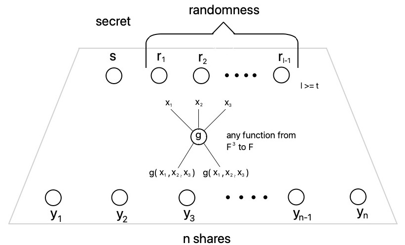
Circuit model. The computation model is that of unrestricted arithmetic circuits over a finite field $\mathbb{F}$, as illustrated in Figure 1. We assume the secret is represented by an element of $\mathbb{F}$, and each share is also an element of $\mathbb{F}$. To realize the distribution of $n$ shares in a $(t,n)$-threshold SS scheme, the circuit has $t$ inputs and $n$ outputs, where one input corresponds to the secret and the remaining $t-1$ inputs are independent random elements of $\mathbb{F}$. The circuit is unrestricted in the sense that each gate can compute any function and has unbounded fan-in. Accordingly, we measure circuit size by the number of wires rather than the number of gates.

Our first result gives a graph-theoretic condition that must be satisfied by any unrestricted arithmetic circuit computing the $n$ shares of a $(t,n)$-threshold SS scheme.

Theorem 1.

An $(t,n)$-concentrator, where $t\leq n$, is a directed acyclic graph with $t$ inputs and $n$ outputs in which every set of $t$ outputs is connected to distinct $t$ inputs by vertex-disjoint paths.

Let $C$ be an unrestricted arithmetic circuit (arbitrary gates, unbounded fan-in) computing the $n$ shares of a $(t,n)$-threshold SS scheme. Assume $C$ has $t$ inputs, consisting of the secret $s$ and $t-1$ random field elements. Then:

• $C$ is a $(t,n)$-concentrator.

• Removing $s$ yields a $(t-1,n)$-concentrator.

Theorem 1 is proved using Shannon-type information inequalities, which is later used to derive circuit lower bounds (see Theorem 3 below). To the best of our knowledge, the use of Shannon-type information inequalities to prove circuit lower bounds is new. Our strategy is to use the well-known entropy characterization of threshold secret sharing (namely, (3) and (4) below) to derive new information inequalities—specifically, Theorem 5 and Theorem 6—via Shannon-type information inequalities, and to relate these inequalities to the connectivity properties of the circuit graph.

In contrast, Newman, Ragde, and Wigderson used graph entropy to prove superlinear lower bounds on the formula size of certain Boolean functions. Beyond this, we are not aware of other techniques that use Shannon-type or non-Shannon-type information inequalities to establish circuit lower bounds.

Our second result establishes a reverse direction that complements Theorem 1. We show that any graph satisfying the conditions of Theorem 1 can be transformed into an arithmetic circuit computing the shares of a threshold SS scheme. Together, Theorem 1 and Theorem 2 give a graph-theoretic characterization of unrestricted arithmetic circuits computing the shares of a threshold SS scheme.

Theorem 2.

Let $G$ be a directed acyclic graph with $t$ inputs and $n$ outputs satisfying the conditions of Theorem 1. We convert $G$ into an arithmetic circuit by replacing each non-input vertex with a weighted addition gate, where the coefficients are chosen independently and uniformly at random from $\mathbb{F}_{q}$. If $q$ is sufficiently large, then with high probability the resulting circuit computes the $n$ shares of a $(t,n)$-threshold SS scheme.

The proof technique originates from network coding [20] and has been applied in several other places. For example, Cheung, Kwok, and Lau used this idea to design fast algorithms for computing the rank of a matrix [11], and Drucker and Li used related ideas to construct circuits encoding error-correcting codes [15]. In [15], Drucker and Li introduced superconcentrator-induced codes whose generator matrices are totally invertible, meaning that every square submatrix is invertible. Such codes can be used to realize threshold secret sharing schemes; in fact, as shown in Theorem 2, a weaker condition already suffices.

The connection between threshold secret sharing and MDS codes was known [19, 9]. We can therefore reformulate our main results in terms of the arithmetic circuit complexity of MDS codes.

Shah, Rashmi, and Ramchandran [28] studied the communication complexity of threshold secret sharing by establishing a necessary condition and a distinct sufficient condition, both expressed in graph-theoretic terms. Their necessary condition coincides with the first condition in Theorem 1; their sufficient condition differs from ours.

As a consequence of the graph-theoretic characterization, we derive asymptotically tight lower bounds on the size of bounded-depth circuits that compute the shares of a threshold SS scheme.

Theorem 3.

Let $\mathbb{F}_{q}$ be a field and let $c\in(0,1)$ be a constant. Let $C:\mathbb{F}_{q}^{t}\to\mathbb{F}_{q}^{n}$, with $t=cn$, be an unrestricted arithmetic circuit of depth $d$ (allowing arbitrary gates and unbounded fan-in) that computes the shares of a $(t,n)$-threshold secret sharing scheme. The inputs consist of the secret together with $t-1$ random elements, and the outputs are the $n$ shares. Then the number of wires in $C$ is at least $\Omega_{d,c}\!\left(\lambda_{d}(n)\cdot n\right)$.

Theorem 3 is proved by combining Theorem 1, the connectivity requirement satisfied by circuits encoding good error-correcting codes as shown by Gál et al. [17] (straightforwardly extended from $\mathbb{F}_{2}$ to a large finite field), and the size bounds for densely regular graphs due to Pudlák [24].

Our next result is a non-explicit construction of unbalanced superconcentrators. The construction follows classical techniques for balanced superconcentrators, such as those in [22, 30, 14].

Theorem 4.

For any $m\geq n$, there exists an $(m,n)$-superconcentrator with $O(m)$ edges and with depth $\alpha(m,n)+O(1)$, where $\alpha(m,n)$ is a version of the two-parameter inverse Ackermann function.

Combining Theorems 2 and 4, we conclude that a $(t,n)$-threshold secret sharing scheme can be implemented by a linear-size circuit of depth $O(\alpha(t,n))$. For instance, depth 2 suffices when $n>t^{2.5}$, and depth 3 suffices when $n>t\log^{1.5}t$.

2 Preliminaries

2.1 Entropy and information inequalities

Let $X$ be a random variable taking values in a finite set, and let $p(x)=\Pr[X=x]$. The entropy of $X$ is

$$H(X)=-\sum_{x}p(x)\log p(x).$$

For random variables $X$ and $Y$, the conditional entropy of $Y$ given $X$ is

$$H(Y\mid X)=-\sum_{x,y}p(x,y)\log p(y\mid x),$$

where $p(y\mid x)=\Pr[Y=y\mid X=x]$. It is well known that

$$H(Y\mid X)=H(X,Y)-H(X)\quad\text{and}\quad H(Y\mid X)=\sum_{x}p(x)H(Y\mid X=x).$$

The mutual information between $X$ and $Y$ is

$$I(X;Y)=\sum_{x,y}p(x,y)\log\frac{p(x,y)}{p(x)p(y)},$$

and satisfies $I(X;Y)=I(Y;X)$ and

$$I(X;Y)=H(X)-H(X\mid Y)\geq 0.$$ (1)

The conditional mutual information of $X$ and $Y$ given $Z$ is

$$I(X;Y\mid Z)=\sum_{x,y,z}p(x,y,z)\log\frac{p(x,y\mid z)}{p(x\mid z)p(y\mid z)},$$

and satisfies

$$I(X;Y\mid Z)=H(X\mid Z)-H(X\mid Y,Z)\geq 0.$$ (2)

A linear information inequality is called Shannon-type if it can be obtained as a nonnegative linear combination of the basic Shannon inequalities, namely the nonnegativity of conditional entropy $H(X\mid Y)\geq 0$ and conditional mutual information $I(X;Y\mid Z)\geq 0$.

We refer to [31] for background on entropy functions and information inequalities.

2.2 Secret sharing scheme

A secret sharing (SS) scheme allows a dealer to distribute a secret among a group of participants such that

• (Correctness) any authorized subset of participants can fully recover the secret, and

• (Privacy) any unauthorized subset of participants learns nothing about the secret.

One widely studied type of SS scheme is the $(t,n)$-threshold SS scheme, in which any subset of $t$ participants (out of $n$ participants) can recover the secret, while any subset of at most $t-1$ participants learns nothing about it.

Fix a finite field $\mathbb{F}$. We represent the secret $s$ as an element of $\mathbb{F}$. (If the secret size is larger than the field size, the secret can be divided into smaller pieces, and the SS scheme can be applied to each piece separately.) Let $r_{1},r_{2},\dots$ be random elements of $\mathbb{F}$ used by the SS scheme, and let $R=\{r_{1},r_{2},\ldots\}$. A scheme is called a linear SS scheme if each share is a linear combination of the secret $s$ and $r_{1},r_{2},\ldots$ over the field $\mathbb{F}$.

It is well known that the requirements of a secret sharing scheme can be characterized using entropy functions [7]. Let the secret be represented by a random variable $S$, and let the $n$ shares be represented by random variables $Y_{1},Y_{2},\ldots,Y_{n}$. The scheme is a $(t,n)$-threshold SS scheme if and only if the following conditions hold:

• (Correctness) For every $T=\{i_{1},\ldots,i_{t}\}\subseteq[n]$ of size $t$,

  $$H(S|Y_{T})=0,$$ (3)

  where $Y_{T}$ denotes the vector $(Y_{i_{1}},\ldots,Y_{i_{t}})$.

• (Privacy) For every $T\subseteq[n]$ of size $t-1$,

  $$H(S|Y_{T})=H(S).$$ (4)

2.3 Arithmetic circuit model

In the arithmetic circuit model, we assume

• The secret is an element of a finite field $\mathbb{F}$.

• During the distribution phase, at most $\ell-1$ random field elements are used, denoted by $r_{1},\ldots,r_{\ell-1}$. Let $R={r_{1},\ldots,r_{\ell-1}}$. (As shown later, any $(t,n)$-threshold SS scheme requires at least $t-1$ random elements.)

• The $n$ shares are computed by an arithmetic circuit over $\mathbb{F}$ with $n$ outputs, denoted by $y_{1},y_{2},\ldots,y_{n}$.

• Gates have unbounded fan-in. The size of the circuit is measured by the number of wires.

• For the lower bounds proved in this work, we assume the arithmetic circuit is unrestricted: a gate with fan-in $d$ may compute an arbitrary function from $\mathbb{F}^{d}$ to $\mathbb{F}$, where $d$ is unbounded.

• For the upper bounds in this work, we assume that each gate is a weighted addition gate. That is, a gate $g(x_{1},\ldots,x_{m})$ with inputs $x_{1},\ldots,x_{m}$ computes

  $$g(x_{1},\ldots,x_{m})=\sum_{i=1}^{m}c_{i}x_{i},$$

  where $c_{1},\ldots,c_{m}\in\mathbb{F}$ are fixed coefficients. Note that a weighted addition gate with $m$ inputs can be realized by first applying $m$ multiplication gates (one per input) followed by a bounded fan-in addition gate, resulting in total size $O(m)$ and depth $2$.

• In a linear SS scheme, the circuit computes a linear transformation $X\mapsto MX$, where $X\in\mathbb{F}^{\ell}$ and $M$ is an $n\times\ell$ matrix. (However, internal gates need not be linear.)

• An arithmetic circuit is called linear if every gate computes a linear function over $\mathbb{F}$. In particular, a linear arithmetic circuit computes a linear transformation.

Figure 1: unrestricted arithmetic circuit computing $n$ shares

2.4 Inverse Ackermann-type function

Following Raz and Shpilka [26], we define slowly-growing functions $\lambda_{d}(n)$. These are inverse Ackermann-type functions that are tailored for superconcentrators.

Definition 1.

For a function $f$, define $f^{(i)}$ to be the composition of $f$ with itself $i$ times, i.e., $f^{(i)}=\underbrace{f\circ f\circ\ldots\circ f}_{i\text{ times}}$. Thus, $f^{(1)}=f$.

For a function $f:\mathbb{N}\to\mathbb{N}$ such that $f(n)<n$ for all $n>1$, define

$$f^{*}(n)=\min\{i:f^{(i)}(n)\leq 1\}.$$

Proposition 1.

Let $f:\mathbb{N}\to\mathbb{N}$ be any function such that $f(n)<n$ for all $n>1$. Then we have

$$f^{*}(n)\leq f(n)-1.$$

Proof.

Consider

$$f^{(1)}(n),\ldots,f^{(i)}(n)=1,$$

where $i=f^{*}(n)$. Since $n>f(n)>f^{(1)}(n)>\ldots>f^{(i)}(n)=1$, we have $i\leq f(n)-1$. ∎

Definition 2.

[26] Let

$$\lambda_{1}(n) = \lfloor\sqrt{n}\rfloor,$$

$$\lambda_{2}(n) = \lceil\log(n)\rceil,$$

$$\lambda_{d}(n) = \lambda_{d-2}^{*}(n),\text{ for }d\geq 3$$

As $d$ increases, the functions $\lambda_{d}(n)$ grow extremely slowly. One can verify the following:

$$\lambda_{2}(n)=\Theta(\log n),\qquad\lambda_{3}(n)=\Theta(\log\log n),\qquad\lambda_{4}(n)=\Theta(\log^{*}n),\qquad\lambda_{5}(n)=\Theta(\log^{*}n).$$

To analyze the size bounds of unbalanced superconcentrators, we require a two-parameter version of the inverse Ackermann function. The constants in the following definition are not optimized.

Definition 3.

[Inverse Ackermann function] For any $m\geq n$, define

$$\alpha(m,n)=\begin{cases}\min\{d:\frac{m}{n}\geq\lambda_{d}(n)\},&\text{if}\ m\geq 128n,\\ \min\{d:\lambda_{d}(n)\leq 4\},&\text{otherwise.}\end{cases}$$ (5)

We denote $\alpha(n,n)$ simply by $\alpha(n)$, which recovers the standard one-parameter inverse Ackermann function.

There exist multiple variants of the Ackermann function in the literature. To the best of our knowledge, all reasonable definitions of the inverse Ackermann function differ only by a multiplicative constant factor.

To show that $\alpha(m,n)$ is well-defined and to facilitate its use in the construction of unbalanced superconcentrators, we require the following properties. Proofs are deferred to Appendix A.

Proposition 2.

1. For any $n\geq 1$,

$$\lambda_{3}(n)\leq\log\log n+2.$$

2. For any $n\geq 1$,

$$\lambda_{4}(n)\leq 2\log^{*}n.$$

3. For any $d\geq 1$, for all $n\geq 4$,

$$\lambda_{d}(n)\leq n-2.$$

Proposition 3.

1. For any $d\geq 1$,

$$\lambda_{d}(d)\leq 4.$$

2. For any $d\geq 1$, if $\lambda_{d}(n)\leq C$, where $C\geq 128$, then

$$\lambda_{d+2}(n)^{2}\leq C.$$

2.5 Superconcentrators and concentrators

An $(m,n)$-network is a directed acyclic graph with $m$ inputs and $n$ outputs.

Definition 4 ($(m,n)$-superconcentrator [30]).

An $(m,n)$-network is an $(m,n)$-superconcentrator if for any subsets $X\subseteq I$ and $Y\subseteq O$ of equal size, there exist $|X|$ vertex-disjoint paths connecting $X$ to $Y$.

In this definition, $m$ and $n$ need not be equal. When $m=n$, tight bounds on the size of bounded-depth superconcentrator are known, achieved in a series of papers.

Depth	Size
2	$\Theta(n\log^{2}n/\log\log n)$ [1, 25]
3	$\Theta(n\log\log n)$ [1]
$d\geq 4$	$\Theta(n\lambda_{d}(n))$ [14, 24]
$\Theta(\alpha(n))$	$\Theta(n)$ [14]

Table 1: Superconcentrator size bounds.

Another relevant concept is concentrators, which are critical building blocks for constructing superconcentrators.

Definition 5 (Concentrator).

An $(m,n,c)$-concentrator is an $(m,n)$-network with the following property: for any $c$ vertices chosen from the smaller of the input and output sets, there exist $c$ vertex-disjoint paths connecting them to $c$ distinct vertices in the other set.

In particular:

• If $m\geq n$, then for any subset of $c$ inputs, there exist $c$ vertex-disjoint paths connecting them to $c$ distinct outputs.

• If $m<n$, then for any subset of $c$ outputs, there exist $c$ vertex-disjoint paths connecting them to $c$ distinct inputs.

An $(m,n,n)$-concentrator or $(m,n,m)$-concentrator is called a full-capacity concentrator, and is simply denoted as an $(m,n)$-concentrator.

Every $(m,n)$-superconcentrator is an $(m,n)$-concentrator. Concentrators serve as building blocks in the construction of superconcentrators.

Using a standard probabilistic argument, one can prove

Lemma 1.

[23, 14] For any integers $m,n,k$ satisfying $n\geq m$, $n\geq 1.1\,k$, and $m\geq k+1$, there exists a depth-1 $(m,n,k)$-concentrator of size

$$O\Bigl(n\cdot\frac{\log(n/k)}{\log(m/k)}\Bigr).$$

3 Characterization via graph-theoretic properties

3.1 Necessity

In this section, we use Shannon’s information measures to show that the connectivity properties must hold for all circuits computing threshold secret-sharing schemes, linear or nonlinear.

The computation model is, again, an unrestricted arithmetic circuit as illustrated by Figure 1, which computes the shares of some $(t,n)$-threshold SS scheme. The inputs are $s$ and $R=\{r_{1},r_{2},\ldots,r_{\ell-1}\}$, where $s\in\mathbb{F}$ is the secret, and $r_{1},\ldots,r_{\ell-1}\in\mathbb{F}$ are independently and uniformly distributed over $\mathbb{F}$; the outputs are $y_{1},\ldots,y_{n}$, representing $n$ shares.

Our goal is to prove that any circuit computing the shares of some $(t,n)$-threshold SS scheme must satisfy

• For any subset of outputs $T\subseteq[n]$ of size $t-1$, there are $t-1$ vertex-disjoint paths connecting $R$ and $T$.

• For any subset of outputs $T\subseteq[n]$ of size $t$, there are $t$ vertex-disjoint paths connecting inputs (i.e., $R\cup\{s\}$) and $T$.

Our strategy is to formulate the connectivity requirements as information inequalities. We rely on two key observations: each gate carries at most $\log|\mathbb{F}|$ units of information; if random variables $Y$ can be written as a function of random variables $X$, then $H(Y)\leq H(X)$. So, it suffices to prove

• For any subset of outputs $T\subseteq[n]$ of size $t-1$,

  $$H(Y_{T}|S)\geq(t-1)H(S).$$ (6)

• For any subset of outputs $T\subseteq[n]$ of size $t$,

  $$H(Y_{T})\geq tH(S).$$ (7)

Given (3) and (4), it turns out inequalities (6) and (7) can be proved using Shannon-type inequalities.

Before proving the information inequalities (6) and (7), we first prove the following lemma.

Lemma 2.

Let $Y_{1},Y_{2},\ldots,Y_{n}$ be random variables. Then

$$\sum_{j\in[n]}H(Y_{[n]\setminus\{j\}})-(n-1)H(Y_{1},\ldots,Y_{n})\geq 0.$$

Proof.

Write

$$\sum_{j\in[n]}H(Y_{[n]\setminus\{j\}})-(n-1)H(Y_{1},\ldots,Y_{n})$$

$$= \sum_{j\in[n]}\left(H(Y_{[n]\setminus\{j\}})-H(Y_{1},\ldots,Y_{n})\right)+H(Y_{1},\ldots,Y_{n}).$$ (8)

By the chain rule

$$H(Y_{1},Y_{2},\ldots,Y_{n})$$

$$= H(Y_{1})+H(Y_{2}|Y_{1})+H(Y_{3}|Y_{1},Y_{2})+\ldots+H(Y_{n}|Y_{1},Y_{2},\ldots,Y_{n-1})$$

$$\geq H(Y_{1}|Y_{[n]\setminus\{1\}})+H(Y_{2}|Y_{[n]\setminus\{2\}})+\ldots+H(Y_{n}|Y_{[n]\setminus\{n\}}),$$

since conditioning reduces entropy. Plugging it into (8), we have

$$\sum_{j\in[n]}H(Y_{[n]\setminus\{j\}})-(n-1)H(Y_{1},\ldots,Y_{n})$$

$$\geq \sum_{j\in[n]}\left(H(Y_{[n]\setminus\{j\}})-H(Y_{1},\ldots,Y_{n})\right)+\sum_{j\in[n]}H(Y_{j}|Y_{[n]\setminus\{j\}})$$

$$= \sum_{j\in[n]}\left(H(Y_{[n]\setminus\{j\}})-H(Y_{1},\ldots,Y_{n})+H(Y_{j}|Y_{[n]\setminus\{j\}})\right)$$

$$= 0.$$

This proves the lemma. ∎

Theorem 5.

Let $S,Y_{1},Y_{2},\ldots,Y_{n}$ be random variables satisfying

• $H(S|Y_{T})=H(S)$ for any $T\subseteq[n]$ of size $t-1$, and

• $H(S|Y_{T})=0$ for any $T\subseteq[n]$ of size $t$.

Then, we have

$$H(Y_{T})\geq tH(S)$$

for any $T\subseteq[n]$ of size $t$.

Proof.

Since the assumptions hold for every subset $T$ of size $t$, it suffices to prove the claim for $T=\{1,...,t\}$, that is, $H(Y_{1},\ldots,Y_{t})\geq tH(S)$.

We decompose $H(Y_{1},\ldots,Y_{t})-tH(S)$ into three nonnegative terms:

$$H(Y_{1},\ldots,Y_{t})-tH(S)$$

$$= \sum_{j\in[t]}\left(H(S,Y_{[t]\setminus\{j\}})-H(Y_{[t]\setminus\{j\}})-H(S)\right)-t\left(H(S,Y_{[t]})-H(Y_{[t]})\right)$$

$$+\sum_{j\in[t]}\left(H(S,Y_{[t]})-H(S,Y_{[t]\setminus\{j\}})\right)+\sum_{j\in[t]}H(Y_{[t]\setminus\{j\}})-(t-1)H(Y_{[t]})$$

$$= \sum_{j\in[t]}\left(H(S|Y_{[t]\setminus\{j\}})-H(S)\right)-tH(S|Y_{[t]})$$ (9)

$$+\sum_{j\in[t]}H(Y_{j}|S,Y_{[t]\setminus\{j\}})$$ (10)

$$+\sum_{j\in[t]}H(Y_{[t]\setminus\{j\}})-(t-1)H(Y_{[t]}).$$ (11)

The first term (9) is zero by our conditions; the second term (10) is nonnegative; the third term (11) is nonnegative by Lemma 2. Thus, we have $H(Y_{1},\ldots,Y_{t})-tH(S)\geq 0$, as desired. ∎

Theorem 6.

Let $S,Y_{1},Y_{2},\ldots,Y_{n}$ be random variables satisfying

• $H(S|Y_{T})=H(S)$ for any $T\subseteq[n]$ of size $t-1$, and

• $H(S|Y_{T})=0$ for any $T\subseteq[n]$ of size $t$.

Then, we have

$$H(Y_{T}|S)\geq(t-1)H(S)$$

for any $T\subseteq[n]$ of size $t-1$.

Proof.

Since the assumptions and the claim are invariant under relabeling, we assume $T=\{1,2,\ldots,t-1\}$ without loss of generality. Write $H(Y_{T}|S)-(t-1)H(S)$ as

$$H(Y_{[t-1]}|S)-(t-1)H(S)$$

$$= H(S,Y_{[t-1]})-tH(S)$$

$$= \sum_{j\in[t-1]}\left(H(S,Y_{[t]})-H(S,Y_{[t]\setminus\{j\}})\right)+\sum_{j\in[t]}\left(H(S,Y_{[t]\setminus\{j\}})-H(Y_{[t]\setminus\{j\}})-H(S)\right)$$

$$-(t-1)\left(H(S,Y_{[t]})-H(Y_{[t]})\right)+\sum_{j\in[t]}H(Y_{[t]\setminus\{j\}})-(t-1)H(Y_{[t]})$$

$$= \sum_{j\in[t-1]}H(Y_{j}|S,Y_{[t]\setminus\{j\}})$$ (12)

$$+\sum_{j\in[t]}\left(H(S|Y_{[t]\setminus\{j\}})-H(S)\right)$$ (13)

$$-(t-1)H(S|Y_{[t]})$$ (14)

$$+\sum_{j\in[t]}H(Y_{[t]\setminus\{j\}})-(t-1)H(Y_{[t]}),$$ (15)

where the term (12) is clearly nonnegative; terms (13) and (14) are zero due to our conditions; term (15) is nonnegative by Lemma 2. Thus, we have $H(Y_{[t-1]}|S)-(t-1)H(S)\geq 0$, as desired. ∎

Theorem 7 (Menger’s Theorem).

Let $G=(V,E)$ be an undirected graph and let $s,t\in V$ be distinct non-adjacent vertices. The size of a minimum $s$–$t$ vertex cut equals the maximum number of pairwise internally vertex-disjoint $s$–$t$ paths.

Now we are ready to prove our first theorem.

Theorem 8 (Theorem 1 restated).

In the above model as illustrated by Figure 1, if the circuit computes the shares of some $(t,n)$-threshold SS scheme, the following conditions are satisfied:

• for any $T\subseteq[n]$ of size $t-1$, there are $t-1$ vertex-disjoint paths connecting $R$ and $T$;

• for any $T\subseteq[n]$ of size $t$, there are $t$ vertex-disjoint paths connecting inputs and $T$.

Proof.

Assume for contradiction that the first condition does not hold. That is, there exists a set $T\subseteq[n]$ of size $t-1$ such that there are at most $t-2$ vertex-disjoint paths from $R$ to $T$. By Menger’s theorem, there exists a vertex set $U$ of size at most $t-2$ whose removal disconnects $R$ from $T$.

By the definition of the cut set $U$, we know that after setting $S$ to a constant, the outputs $Y_{T}$ can be written as functions in the gates in $U$. Since each gate value lies in $\mathbb{F}$ and hence carries at most $\log|\mathbb{F}|$ bits of entropy, we have

$$H(Y_{T}|S=s)\leq|U|\log|\mathbb{F}|\leq(t-2)\log|\mathbb{F}|.$$

Thus,

$$H(Y_{T}|S)= \sum_{s}\Pr[S=s]H(Y_{T}|S=s)$$

$$\leq \sum_{s}\Pr[S=s](t-2)\log|\mathbb{F}|$$

$$= (t-2)\log|\mathbb{F}|.$$

On the other hand, by Theorem 6, we have

$$H(Y_{T}\mid S)\geq(t-1)H(S)=(t-1)\log|\mathbb{F}|,$$

since $S$ is uniformly distributed over $\mathbb{F}$. This is a contradiction.

The second condition can be proved similarly using Theorem 5. ∎

In other words, the circuit, viewed as a graph, is an $(|R|+1,n,t)$-concentrator; moreover, after removing the input $s$ (along with its incident edges), the remaining graph is an $(|R|,n,t-1)$-concentrator.

3.2 Sufficiency

Given any $(t,n)$-superconcentrator $G$, or more generally any $(t,n)$-network satisfying the conditions of Theorem 1, we construct a $(t,n)$-threshold secret-sharing scheme. The scheme is linear over a sufficiently large finite field $\mathbb{F}$, chosen such that $|\mathbb{F}|\gg d\binom{n}{t},$ where $d$ denotes the depth of the superconcentrator.

Figure 2: linear arithmetic circuit realizing SS distribution

The SS scheme has the following 3 phases:

Setup: Convert $G$ into an arithmetic circuit $C$ over field $\mathbb{F}$ by

• replacing each vertex with an addition gate, and

• for every edge $e$, choosing a coefficient $c_{e}\in\mathbb{F}$ uniformly at random.

One can easily check this linear arithmetic circuit computes a linear transformation $x\mapsto Mx$, where $M=(m_{ij})$ is a $n\times t$ matrix. Here

$$m_{i,j}=\sum_{v_{1}=x_{j},v_{2},\ldots,v_{\ell}=y_{i}}\prod_{k=1}^{\ell-1}c_{(v_{k},v_{k+1})}$$

where the sum ranges over all paths from input $x_{j}$ to output $y_{i}$.

Sharing: Assign the secret $s$ to input $x_{1}$, and choose $x_{2},\ldots,x_{t}$ uniformly at random. For every $i\in[n]$, send the $i$th output of the circuit to participant $P_{i}$. In other words,

$$\begin{pmatrix}y_{1}\\ y_{2}\\ \vdots\\ y_{n}\end{pmatrix}=M\begin{pmatrix}s\\ r_{2}\\ \vdots\\ r_{t}\end{pmatrix},$$

where $s\in\mathbb{F}$ is the secret, and $r_{2},\ldots,r_{t}$ are uniformly random elements over $\mathbb{F}$.

Reconstruction: Consider any coalition of $t$ participants $T\subseteq[n]$ with shares denoted by

$$Y_{T}=M_{T}X=M_{T}\begin{pmatrix}s\\ r_{2}\\ \vdots\\ r_{t}\end{pmatrix},$$

where $X=(s,r_{2},\ldots,r_{t})^{T}$, and $M_{T}$ is the $t\times t$ submatrix of $M$ formed by rows indexed by $T$ and all columns. Assuming $M_{T}$ is invertible (which will be proved), we have $X=M_{T}^{-1}Y_{T}$. The secret $s$ is then recovered as the first coordinate of $M_{T}^{-1}Y_{T}$.

Lemma 3.

With probability at least $1-\frac{d\binom{n}{t}}{|\mathbb{F}|}$, the secret can be recovered by any set of $t$ participants.

Proof.

It suffices to show that, with probability at least $1-\frac{d\binom{n}{t}}{|\mathbb{F}|}$, for all $T\subseteq[n]$ of size $t$, $\det(M_{T})\neq 0$. Because if $M_{T}$ is invertible, we can recover the secret by computing $X=M_{T}^{-1}Y_{T}$, where $Y_{T}$ denotes the shares received by the $t$ participants.

Claim 1.

For any $T\subseteq[n]$ of size $t$, we have

$$\Pr[\det(M_{T})=0]\leq\frac{d}{|\mathbb{F}|}.$$

Proof.

(of the Claim) Viewing the coefficients $c_{e}$ as the indeterminates, $\det(M_{T})$ is a polynomial in $\mathbb{F}[\{c_{e}:e\in E(G)\}]$.

Note that there are $t$ vertex-disjoint paths from inputs to $T$. Setting the coefficients along these $t$ vertex-disjoint paths to $1$, and all other coefficients to $0$, the determinant evaluates to $\pm 1$. Hence, $\det(M_{T})$ is a nonzero polynomial.

Observe that the polynomial $\det(M_{T})$ has total degree $\leq d$, where $d$ is the depth of the circuit. By Schwartz-Zippel Lemma, we have

$$\Pr[\det(M_{T})=0]\leq\frac{\deg(\det(M_{T}))}{|\mathbb{F}|}\leq\frac{d}{|\mathbb{F}|}.$$

∎

By the union bound over all $\binom{n}{t}$ choices of $T$, the probability that $\det(M_{T})\neq 0$ for all $T$ is at least $1-\frac{d\binom{n}{t}}{|\mathbb{F}|}$, as claimed. ∎

Lemma 4.

With probability at least $1-\frac{d\binom{n}{t-1}}{|\mathbb{F}|}$, any set of $t-1$ participants receives no information about the secret.

Proof.

Let $M_{T,\{2,3,\ldots,t\}}$ denote the $|T|\times(t-1)$ matrix indexed by rows $T$ and columns $2,3,\ldots,t$, where $T\subseteq[n]$. For any $T\subseteq[n]$ of size $t-1$, we claim

$$\Pr[\det M_{T,\{2,3,\ldots,t\}}=0]\leq\frac{d}{|\mathbb{F}|}.$$

Viewing the coefficients $c_{e}$ as indeterminates over $\mathbb{F}$, $\det M_{T,\{2,3,\ldots,t\}}$ is a polynomial in $\{c_{e}:e\in E(G)\}$ of degree at most $d$. Since the circuit graph satisfies the second condition in Theorem 1, there exist $t-1$ vertex-disjoint paths connecting the inputs $x_{2},\ldots,x_{t}$ to the outputs in $T$. Setting the coefficients $c_{e}$ along these $t-1$ vertex-disjoint paths to $1$, and all other coefficients to $0$, the determinant evaluates to $\pm 1$, so $\det M_{T,\{2,3,\ldots,t\}}$ is a nonzero polynomial. The claim follows from Schwartz-Zippel Lemma.

Taking a union bound over all $T\subseteq[n]$ of size $t-1$, we know with probability at least $1-\frac{d{n\choose t-1}}{|\mathbb{F}|}$, $\det M_{T,\{2,3,\ldots,t\}}\not=0$ for all $T$.

Consider any $t-1$ participants indexed by $T$, who receive the following vector in the reconstruction phase

$$y_{T} = M_{T,[t]}\begin{pmatrix}s\\ r_{2}\\ \vdots\\ r_{t}\end{pmatrix}$$

$$= \begin{pmatrix}M_{T,1}&M_{T,\{2,\ldots,t\}}\end{pmatrix}\begin{pmatrix}s\\ R\end{pmatrix}$$

$$= M_{T,1}s+M_{T,\{2,\ldots,t\}}R,$$

where $R=\begin{pmatrix}r_{2}\\ \vdots\\ r_{t}\end{pmatrix}$.

Since $M_{T,\{2,\ldots,t\}}$ is of full rank, we know $M_{T,\{2,\ldots,t\}}R$ is uniformly distributed in $\mathbb{F}^{t-1}$ when $R\in\mathbb{F}^{t-1}$ is uniformly distributed. Thus $M_{T,1}s+M_{T,\{2,\ldots,t\}}R$ is uniformly distributed over $\mathbb{F}^{t-1}$, independent of $s$. Hence, any $t-1$ participants indexed by $T$ obtain zero information about the secret. ∎

Theorem 2 immediately follows from Lemmas 3 and 4.

The graph-theoretic condition required is slightly weaker than that of a superconcentrator; in fact, a concentrator suffices. For instance, consider a $(t-1,n)$-concentrator, add an additional input node $s$, and connect $s$ directly to all $n$ outputs. With this modification, the two connectivity conditions described above are satisfied.

4 Consequences

4.1 Size lower bounds

Definition 6.

(Densely regular graph [24]) Let $G$ be a directed acyclic graph with $n$ inputs and $n$ outputs. Let $0<\epsilon,\delta$ and $0\leq\mu\leq 1$. We say $G$ is $(\epsilon,\delta,\mu)$-densely regular if for every $k\in[\mu n,n]$, there are probability distributions $\mathcal{X}$ and $\mathcal{Y}$ on $k$-element subsets of inputs and outputs respectively, such that for every $i\in[n]$,

$$\Pr_{X\in\mathcal{X}}[i\in X]\leq\frac{k}{\delta n}\text{ and }\Pr_{Y\in\mathcal{Y}}[i\in Y]\leq\frac{k}{\delta n}$$

and the expected number of vertex-disjoint paths from $X$ to $Y$ is at least $\epsilon k$ for randomly chosen $X\in\mathcal{X}$ and $Y\in\mathcal{Y}$.

Denote by $D(n,d,\epsilon,\delta,\eta)$ the minimal size of a $(\epsilon,\delta,\mu)$-densely regular layered directed acyclic graph with $n$ inputs and $n$ outputs and depth $d$.

The following result was proved for the case $\mathbb{F}_{2}$ (Lemma 3 in [17]); extending it to any finite field $\mathbb{F}_{q}$ is straightforward.

Lemma 5.

Let $\mathbb{F}_{q}$ be the finite field of size $q$. Let $\delta>0$ be a constant. Let $C:\mathbb{F}_{q}^{m}\to\mathbb{F}_{q}^{n}$ be a code with minimum distance $\delta n$ and $G$ be an unrestricted arithmetic circuit (with arbitrary gates and unbounded fan-in computing $C$. For any $k\in\{1,\ldots,m\}$, and for any $k$-element subset $X$ of inputs of $G$, if we take uniformly at random a $k$-element subset $Y$ of outputs of $G$, then the expected number of vertex-disjoint paths from $X$ to $Y$ in $G$ is at least $\delta k$.

Corollary 1.

(Corollary 15 in [17]) Let $0<\rho,\delta<1$ be constants and let $C:\mathbb{F}_{q}^{\rho n}\to\mathbb{F}_{q}^{n}$ be a circuit computing a code with relative distance $\delta$. If we extend the circuit by $(1-\rho)n$ dummy inputs, then its underlying graph is $(\rho\delta,\rho,\tfrac{1}{n})$-densely regular.

Corollary 1 directly follows from Lemma 5.

Lemma 6.

Let $G$ be a $(cn,n,cn)$-concentrator, where $c\in(0,1)$ is a constant. Then, after adding $(1-c)n$ dummy inputs, the graph is $(c(1-c),c,\tfrac{1}{n})$-densely regular.

Proof.

The proof proceeds in three steps.

1. First, over a sufficiently large field, we transform the graph into a linear arithmetic circuit that computes a code of relative distance $1-c$.

2. Second, by Lemma 5, we know that any arithmetic circuit computing a code with relative distance $1-c$ satisfies the connectivity requirement of Lemma 5.

3. Third, by applying Corollary 1, we conclude that the graph is densely regular.

Let $\mathbb{F}_{q}$ be a finite field, where $q$ is sufficiently large. We convert the $(cn,n,cn)$-concentrator graph $G$ into a linear arithmetic circuit, where each vertex replaced a weighted addition gate with random coefficients. Let $C:\mathbb{F}_{q}^{cn}\to\mathbb{F}_{q}^{n}$ be the linear mapping computed by the circuit, which computes a linear transformation $C(x)=Hx$, where $H$ is an $n\times cn$ matrix, and $x\in\mathbb{F}_{q}^{cn}$.

We claim that there exists a circuit $C(x)=Hx$ such that, for every subset $S\subseteq[n]$ with $|S|=cn$, the row submatrix $H_{S}$ has full rank. Indeed, for any fixed $S$, the determinant $\det(H_{S})$ is a nonzero polynomial of degree at most the depth of the graph $G$. By the definition of a $(cn,n,cn)$-concentrator, there exist $cn$ vertex-disjoint paths connecting the $cn$ inputs to the vertices in $S$, which guarantees that $\det(H_{S})$ is not identically zero. Therefore, by the Schwartz–Zippel lemma,

$$\Pr[\det(H_{S})=0]\leq\frac{d}{q},$$

where $d$ denotes the depth of the graph $G$.

Fix such a code $C$. We claim that $C$ has relative distance at least $1-c$. Let $x\in\mathbb{F}_{q}^{cn}$ be any nonzero vector. For any subset $S\subseteq[n]$ with $|S|=cn$, the submatrix $C_{S}$ has full rank, and hence $C(x)_{S}=xC_{S}\neq\vec{0}$. Therefore, no nonzero codeword can be zero on more than $cn-1$ coordinates, which implies that the Hamming weight of $C(x)$ is at least $n-cn+1$.

The second step follows from Lemma 5, and the third step follows from Corollary 1.

∎

Theorem 9.

[24] Let $\epsilon,\delta>0$ be constants. Then for every $n$, $\mu\in[1/n,1]$, and $d\geq 3$, we have

$$D(n,d,\epsilon,\delta,\mu)\geq\Omega_{d,\epsilon,\delta}(n\cdot\lambda_{d}(1/\mu)).$$

Theorem 10 (Theorem 3).

Let $\mathbb{F}_{q}$ be a field and let $c\in(0,1)$ be a constant. Let $C:\mathbb{F}_{q}^{t}\to\mathbb{F}_{q}^{n}$, with $t=cn$, be an unrestricted arithmetic circuit of depth $d$ (allowing arbitrary gates and unbounded fan-in) that computes the shares of a $(t,n)$-threshold secret sharing scheme. The inputs consist of the secret together with $t-1$ random elements, and the outputs are the $n$ shares. Then the number of wires in $C$ is at least $\Omega_{d,c}\!\left(\lambda_{d}(n)\cdot n\right)$.

Proof.

By Theorem 1, the circuit $C$, viewed as a graph $G$, is a $(cn,n,cn)$-concentrator. By Lemma 6, the graph $G$ is $(c(1-c),\,c,\,1/n)$-densely regular. Finally, Theorem 9 implies that $G$ has size $\Omega_{d,c}\!\left(\lambda_{d}(n)\cdot n\right)$. ∎

4.2 Size upper bounds

Let $\mathrm{SC}_{d}(m,n)$ denote the minimum size of a depth-$d$ superconcentrator with $m$ inputs and $n$ outputs, where $m$ and $n$ need not be equal ($m$ may be larger or smaller than $n$).

For computing SS schemes, we need unbalanced superconcentrators, where the number of inputs is the threshold value $t$, and the number of outputs is the number of participants $n$.

From Table 1, we know there exists a linear-size $(n,n)$-superconcentrator of depth $O(\alpha(n))$. By removing some inputs (and the incident edges), we obtain an $O(n)$-size $(m,n)$-superconcentrator depth $O(\alpha(n))$, for any $m\leq n$. Size $O(n)$ is clearly optimal (up to a multiplicative constant), since at least $n$ edges are required to connect the $n$ outputs. The question is, given $m,n$, can we achieve a depth smaller than $O(\alpha(n))$ for an $(m,n)$-superconcentrator?

Definition 7 (Partial superconcentrator [14]).

An $(m,n)$-network is a $(p,q)$-partial superconcentrator if for any $S\subseteq[m]$ and $T\subseteq[n]$ with $|S|=|T|$ and $|S|\in[q,p]$, there exist $|S|-q$ vertex-disjoint paths connecting $S$ and $T$.

Let $\mathrm{SC}_{d}(m,n,p,q)$ denote the minimal size of an $(m,n)$-network of depth at most $d$ which is a $(p,q)$-partial superconcentrator.

4.3 Depth 2

In this subsection, we construct unbalanced superconcentrators of depth 2, which are used as building blocks for higher depth.

Lemma 7.

For any $r$, we have

$$\mathrm{SC}_{2}(n,m,n/r,2n/(3r))=O(m\log m).$$

Proof.

As illustrated in Figure 3, we construct a depth-2 network with $n$ inputs, $m$ outputs, and a middle layer containing $4n/(3r)$ vertices. The construction consists of two layers:

• Top layer: $(n,4n/(3r),n/r)$-concentrator;

• Bottom layer: $(m,4n/(3r),n/r)$-concentrator.

Figure 3: Construction of depth-2 superconcentrator

Consider $S\subseteq[n]$ and $T\subseteq[m]$ of size $2n/(3r)+\Delta$, where $0\leq\Delta\leq n/(3r)$. By the definition of the top-layer $(n,4n/(3r),n/r)$-concentrator, $S$ is connected to $|S|$ vertices in the middle layer, denoted by $S^{\prime}$. Similarly, $T$ is connected to $|T|$ vertices in the middle layer, denoted by $T^{\prime}$. Then

$$|S^{\prime}\cap T^{\prime}|\geq|S^{\prime}|+|T^{\prime}|-4n/(3r)=2\Delta.$$

Thus, $S$ and $T$ are connected by $2\Delta$ vertex-disjoint paths (in fact, $\Delta$ paths suffice to satisfy the partial superconcentrator condition). Therefore, the $(n,m)$-network is a $(n/r,2n/(3r))$-partial superconcentrator. ∎

By taking the union of $O(\log n)$ partial superconcentrators, we obtain the following upper bound on depth-2 superconcentrators.

Lemma 8.

For any $n\leq m$, we have

$$\mathrm{SC}_{2}(n,m)=O(m\log m\cdot\log n).$$

Proof.

Let

$$r=\left(\frac{3}{2}\right)^{0},\left(\frac{3}{2}\right)^{1},\ldots,\left(\frac{3}{2}\right)^{\ell},\quad\text{where }\ell=\log_{3/2}n-1.$$

This gives a sequence of partial superconcentrators

$$\left(n,\frac{2n}{3}\right),\left(\frac{2n}{3},\frac{4n}{9}\right),\ldots,\left(\frac{n}{(3/2)^{\ell-1}},\frac{n}{(3/2)^{\ell}}\right),$$

each of size $O(m\log m)$ by Lemma 7.

By combining these $\ell=O(\log n)$ partial superconcentrators and merging their inputs and outputs, we obtain an $(n,m)$-superconcentrator of size $O(m\log m\cdot\log n)$. ∎

When $m\geq n^{2+\Omega(1)}$, we prove there exists a depth-2 $(m,n)$-superconcentrator of linear size.

Lemma 9.

For any $\epsilon>0$, if $m\geq n^{2+\epsilon}$,

$$\mathrm{SC}_{2}(m,n)=O\left(\frac{m}{\epsilon}\right).$$

Proof.

Construct a depth-2 $(m,n)$-network as illustrated in Figure 4. Let the middle layer contain $\frac{m}{r}$ vertices, where

$$r=\left(\frac{m}{n}\right)^{\frac{1}{1+\epsilon}}.$$

• The top layer is a complete bipartite graph connecting all $n$ inputs to the middle layer vertices.

• The bottom layer is a $(m,\frac{m}{r},n)$-concentrator.

Figure 4: Construction of linear-size depth-2 superconcentrator

Correctness: For any subset of outputs $Y$ with $|Y|\leq n$, the bottom-layer $(m,\frac{m}{r},n)$-concentrator connects $Y$ to $|Y|$ middle-layer vertices. These middle-layer vertices are connected to any chosen $|Y|$ inputs via the complete bipartite top layer. Hence the network is indeed an $(m,n)$-superconcentrator.

Size estimation: The top-layer complete bipartite graph has size

$$n\cdot\frac{m}{r}=n\cdot m\cdot\left(\frac{n}{m}\right)^{\frac{1}{1+\epsilon}}=m\cdot\left(\frac{n^{2+\epsilon}}{m}\right)^{\frac{1}{1+\epsilon}}\leq m,$$

since $m\geq n^{2+\epsilon}$.

By Lemma 1, the bottom-layer $(m,\frac{m}{r},n)$-concentrator has size

$$O\left(m\frac{\log(r^{1+\epsilon})}{\log(r^{\epsilon})}\right)=O\left(\frac{m}{\epsilon}\right).$$

Thus the total size is $O(m)+O\left(\frac{m}{\epsilon}\right)=O\left(\frac{m}{\epsilon}\right).$ ∎

4.4 Depth 3

When $m\geq n(\log n)^{2+\Omega(1)}$, we prove there exists a depth-3 $(m,n)$-superconcentrator of linear size.

Lemma 10.

For any $\epsilon>0$, if $m\geq n(\log n)^{2+\epsilon}$,

$$\mathrm{SC}_{3}(m,n)=O\left(\frac{m}{\epsilon}\right).$$

Proof.

If $m\geq n^{3}$, by Lemma 9, we have

$$\mathrm{SC}_{3}(m,n)\leq\mathrm{SC}_{2}(m,n)=O(m).$$

Assume $m<n^{3}$ from now on.

Figure 5: Construction of linear-size depth-3 superconcentrator

We construct an $(n,m)$-network consisting of two parts (Figure 5):

• The top part is a depth-2 $(n,m/r)$-superconcentrator.

• The bottom part is a $(m,m/r,n)$-concentrator, where

  $$r=\left(\frac{m}{n}\right)^{\frac{1}{1+\epsilon/2}}.$$

Correctness: Consider any subsets $X\subseteq[n]$ and $Y\subseteq[m]$ with $|X|=|Y|$. The bottom-layer $(m,m/r,n)$-concentrator connects $Y$ to $|Y|$ middle-layer vertices $Z$. The top-layer $(n,m/r)$-superconcentrator provides $|X|$ vertex-disjoint paths from $X$ to $Z$. Thus there are $|X|$ vertex-disjoint paths connecting $X$ and $Y$.

Size estimation: By Lemma 8, the top-layer depth-2 $(n,m/r)$-superconcentrator has size

$$O\left(\frac{m}{r}\cdot\log\frac{m}{r}\cdot\log n\right)\leq O\left(\frac{m}{r}(\log n)^{2}\right)=O(m),$$

since $\frac{m}{n}\geq(\log n)^{2+\epsilon}$ implies $(m/n)^{1/(1+\epsilon/2)}\geq(\log n)^{2}$.

By Lemma 1, the bottom-layer $(m,m/r,n)$-concentrator has size

$$O\left(m\frac{\log(r^{1+\epsilon/2})}{\log(r^{\epsilon/2})}\right)=O\left(\frac{m}{\epsilon}\right).$$

Hence the total size is $O(m)+O\left(\frac{m}{\epsilon}\right)=O\left(\frac{m}{\epsilon}\right)$. ∎

4.5 Higher depth

As we have shown, when $m\geq n^{2+\epsilon}$ for some constant $\epsilon>0$, depth 2 suffices to achieve linear size; when $m\geq n(\log n)^{2+\epsilon}$, depth 3 suffices; and when $m$ is only “slightly larger” than $n$, higher depth is required.

In this subsection, we prove that for any $m\geq n$, depth $\alpha(m,n)+O(1)$ suffices, where $\alpha(m,n)$ denotes the two-parameter inverse Ackermann function (Definition 3).

Lemma 11.

For any depth $d\geq 3$, the size of a depth-$d$ $(m,n)$-superconcentrator satisfies

$$\mathrm{SC}_{d}(m,n)=O(m\,\lambda_{d}(n)).$$

Proof.

We consider two cases for $m$.

Case 1: $m\geq n^{2.5}$.

By Lemma 9, depth 2 suffices to construct an $(m,n)$-superconcentrator of size $O(m)$. Since increasing depth cannot increase size, for any $d\geq 2$ we have

$$\mathrm{SC}_{d}(m,n)\leq\mathrm{SC}_{2}(m,n)=O(m)=O(m\,\lambda_{d}(n)).$$

Case 2: $m\leq n^{2.5}$.

Observe that, by monotonicity of $\lambda_{d}$,

$$\lambda_{d}(m)\leq\lambda_{d}(n^{2.5}).$$

If $d=3$, $\lambda_{3}(n^{2.5})=O(\log\log n^{2.5})=O(\log\log n)=O(\lambda_{3}(n))$. If $d\geq 4$, by the definition of $\lambda_{d}$ (iterated $\lambda_{d-2}$):

$$\lambda_{d}(n^{2.5})=\min\{i:\lambda_{d-2}^{(i)}(n^{2.5})\leq 1\}=\lambda_{d}(\lambda_{d-2}(n^{2.5}))+1\leq\lambda_{d}(\lceil 2.5\log n\rceil)+1\leq\lambda_{d}(n)+1=O(\lambda_{d}(n)),$$

where we used $\lambda_{2}(n)=\log n$ and the monotonicity of $\lambda_{d}$ in the last step.

Hence, in all cases we have

$$\lambda_{d}(m)\leq O(\lambda_{d}(n)).$$

Finally, from Table 1, there exists a depth-$d$ superconcentrator with $m$ inputs and $m$ outputs of size $O(m\,\lambda_{d}(m))$. By removing $m-n$ outputs and their incident edges, we obtain an $(m,n)$-superconcentrator. Thus,

$$\mathrm{SC}_{d}(m,n)\leq\mathrm{SC}_{d}(m,m)=O(m\,\lambda_{d}(m))\leq O(m\,\lambda_{d}(n)),$$

as desired. ∎

Theorem 11.

For depth $d\geq 3$, if

$$m\geq n\,(\lambda_{d}(n))^{1+\epsilon}$$

for some $\epsilon>0$, then the minimal size of a depth-$(d+1)$ $(n,m)$-superconcentrator satisfies

$$S_{d+1}(m,n)=O\left(\frac{m}{\epsilon}\right).$$

Proof.

We construct a depth-$(d+1)$ $(n,m)$-superconcentrator as follows.

Construction:

• Let $r=\left(\frac{m}{n}\right)^{\frac{1}{1+\epsilon}}$, so that $\frac{m}{r^{1+\epsilon}}=n$.

• Place $\frac{m}{r}$ vertices on the second-to-last layer.

• The first $d$ layers form an $(n,\frac{m}{r})$-superconcentrator.

• The last layer is a $(m,\frac{m}{r},n)$-concentrator connecting the second-to-last layer to the outputs.

Verification: Consider any subset of inputs $X\subseteq[n]$ and outputs $Y\subseteq[m]$ of equal size $|X|=|Y|$. By the definition of the $(m,\frac{m}{r},n)$-concentrator, each output in $Y$ can be connected to a distinct vertex in the second-to-last layer via vertex-disjoint edges; denote these vertices by $Z$. By the definition of the $(n,\frac{m}{r})$-superconcentrator, each input in $X$ can be connected to a distinct vertex in $Z$ via vertex-disjoint paths in the first $d$ layers.

Combining these two sets of vertex-disjoint paths, we obtain $|X|=|Y|$ vertex-disjoint paths connecting $X$ to $Y$. Hence, the constructed network is indeed an $(n,m)$-superconcentrator.

Size estimate: By Lemma 11, the first $d$ layers (depth-$d$ $(n,\frac{m}{r})$-superconcentrator) have size

$$O\Big(\frac{m}{r}\cdot\lambda_{d}(n)\Big)=O\Big(m\cdot\frac{\lambda_{d}(n)}{(\frac{m}{n})^{1/(1+\epsilon)}}\Big).$$

Using the assumption $m\geq n(\lambda_{d}(n))^{1+\epsilon}$, we have

$$\frac{\lambda_{d}(n)}{(\frac{m}{n})^{1/(1+\epsilon)}}\leq 1,$$

so the first $d$ layers contribute $O(m)$ to the total size.

By Lemma 1, the last layer ($(m,\frac{m}{r},n)$-concentrator) has size

$$O\left(m\cdot\frac{\log(r^{1+\epsilon})}{\log(r^{\epsilon})}\right)=O\left(\frac{m}{\epsilon}\right).$$

Total size: Adding the contributions from all layers gives $S_{d+1}(m,n)=O\left(m+\frac{m}{\epsilon}\right)=O\left(\frac{m}{\epsilon}\right),$ absorbing the $O(m)$ term into $O(m/\epsilon)$ since $\epsilon<1$. ∎

Theorem 12 (4).

For any $m\geq n$, if the depth satisfies $d\geq\alpha(m,n)+3,$ then the minimal size of a depth-$d$ $(m,n)$-superconcentrator is linear in $m$, that is, $\mathrm{SC}_{d}(m,n)=O(m),$ where $\alpha(m,n)$ is the two-parameter inverse Ackermann function (Definition 3).

Proof.

Case 1: $m\geq 128\,n$.

By the definition of $\alpha(m,n)$, we have $\frac{m}{n}\geq\lambda_{\alpha(m,n)}(n),$ and by Proposition 3, this implies $\frac{m}{n}\geq\lambda_{\alpha(m,n)+2}^{2}(n).$ Then, applying Theorem 11 with depth $d=\alpha(m,n)+3$, we conclude $\mathrm{SC}_{\alpha(m,n)+3}(m,n)=O(m).$

Case 2: $n\leq m<128\,n$. If $\alpha(m,n)=1$, we have $m\geq n\lfloor\sqrt{n}\rfloor$. By Lemma 10, we know $\mathrm{SC}_{4}(m,n)\leq\mathrm{SC}_{3}(m,n)=O(m)$. If $\alpha(m,n)=2$, we have $m\geq n\log n\geq n(2\log^{*}n)^{2}$. By Theorem 11, $\mathrm{SC}_{5}(m,n)=O(m)$.

From now on, we assume $\alpha(m,n)\geq 3$. By the definition of $\alpha(m,n)$, we have $\lambda_{\alpha(m,n)}(n)\leq 4$. By Lemma 11, we have

$$\mathrm{SC}_{\alpha(m,n)}(m,n)=O(m\lambda_{\alpha(m,n)}(n))=O(m).$$

∎

5 Conclusion

In this paper, we study the arithmetic circuit complexity of threshold secret sharing. We prove a graph-theoretic characterization of unrestricted arithmetic circuits that compute the shares of a threshold secret sharing scheme, when the underlying field is sufficiently large. As a result, we derive both lower and upper bounds.

Appendix A Properties of inverse Ackermann function

We include here the proofs of Proposition 2 and 3.

Proof.

(of Proposition 2) 1. Recall that $\lambda_{1}(n)=\lfloor\sqrt{n}\rfloor$. We have

$$\lambda_{3}(n) \leq \min\{d:n^{2^{-d}}\leq 3\}+1$$

$$= \lceil\log\left(\log n-\log 3\right)\rceil+1$$

$$\leq \log\left(\log n-\log 3\right)+2$$

$$\leq \log\log n+2.$$

2. Recall that $\lambda_{2}(n)=\lceil\log n\rceil<\log n+1$. Let $g(n)=\log n+1$. Observe that $g(g(n))\leq\log n$ for all $n\geq 8$. So we have

$$\lambda_{4}(n) \leq \min\{d:g^{(d)}(n)\leq 8\}+3$$

$$\leq \min\{d:\log^{(\lfloor d/2\rfloor)}(n)\leq 8\}+3.$$

If $\log^{(\lfloor d/2\rfloor)}(n)\leq 8$, then $\log^{(\lfloor d/2\rfloor+2)}(n)\leq\log 3\approx 1.58$. So, $\lfloor\frac{d}{2}\rfloor+2\leq\log^{*}n$, which implies that $d\leq 2(\log^{*}n-2)+1$. Thus $\lambda_{4}(n)\leq 2((\log^{*}n)-2)+1+3=2\log^{*}n$, which holds when $n\geq 8$. When $n\in\{3,4,\ldots,7\}$, $\lambda_{4}(n)\leq 2\log^{*}n$ can be verified by direct computation.

3. We do induction on $d$.

When $d=1$, $\lambda_{d}(n)=\lambda_{1}(n)=\lfloor\sqrt{n}\rfloor\leq n-2$ for all $n\geq 4$.

When $d=2$, $\lambda_{d}(n)=\lambda_{2}(n)=\lceil\log n\rceil\leq n-2$ for all $n\geq 4$.

When $d\geq 3$, $\lambda_{d}(n)=\lambda^{*}_{d-2}(n)\leq\lambda_{d-2}(n)\leq n-2$, where $\lambda^{*}_{d-2}(n)\leq\lambda_{d-2}(n)$ is by induction hypothesis. ∎

Proof.

(of Proposition 3) 1. When $d=1$, $\lambda_{1}(1)=1$; When $d=2$, $\lambda_{2}(2)=1$; When $d=3$, $\lambda_{3}(3)=\lambda_{1}^{*}(3)=1$.

We do induction on $d$, where $d\geq 2$. Assuming the conclusion is true for $d$, we prove it for $d+2$.

$$\lambda_{d+2}(d+2) = \lambda_{d}^{*}(d+2)$$

$$\leq \lambda_{d}^{*}(\lambda_{d}(d+2))+1$$

$$\leq \lambda_{d}^{*}(d)+1,$$

where $\lambda_{d}(d+2)\leq d$ is by Proposition 2. So, $\lambda_{d+2}(d+2)\leq\lambda_{d}^{*}(d)+1\leq\lambda_{d}^{*}(\lambda_{d}(d))+2\leq\lambda^{*}_{d}(4)+2\leq\max\{\lambda_{2}^{*}(4),\lambda_{3}^{*}(4)\}+2=4$.

2. By the definition of $\lambda_{d+2}(n)$, we have $\lambda_{d+2}(n)=\lambda_{d}^{*}(n)\leq\lambda_{d}^{*}(\lambda_{d}(n))+1\leq\lambda_{d}^{*}(C)+1$.

When $d$ is odd, $\lambda_{d}^{*}(C)\leq\lambda_{1}^{*}(C)\leq\log\log C+2$ by Proposition 2. When $C\geq 128$, we have $(\log\log C+2)^{2}\leq C$.

When $d$ is even, $\lambda_{d}^{*}(C)\leq\lambda_{2}^{*}(C)\leq 2\log^{*}C$ by Proposition 2. When $C\geq 128$, we have $(2\log^{*}C+1)^{2}\leq C$. ∎

References

- [1] (1994) Superconcentrators of depths 2 and 3; odd levels help (rarely). J. Comput. Syst. Sci. 48 (1), pp. 194–202. Cited by: Table 1, Table 1.
- [2] (2019) Secret-sharing schemes for general and uniform access structures. In Advances in Cryptology–EUROCRYPT 2019: 38th Annual International Conference on the Theory and Applications of Cryptographic Techniques, Darmstadt, Germany, May 19–23, 2019, Proceedings, Part III, pp. 441–471. Cited by: §1.
- [3] (2020) Better secret sharing via robust conditional disclosure of secrets. In Proceedings of the 52nd Annual ACM SIGACT Symposium on Theory of Computing, pp. 280–293. Cited by: §1.
- [4] (1983) A modular approach to key safeguarding. IEEE transactions on information theory 29 (2), pp. 208–210. Cited by: §1.
- [5] (1999) Superpolynomial lower bounds for monotone span programs. Combinatorica 19 (3), pp. 301–319. Cited by: §1.
- [6] (1996) Secure schemes for secret sharing and key distribution. Cited by: §1.
- [7] (2011) Secret-sharing schemes: a survey. In International conference on coding and cryptology, pp. 11–46. Cited by: §2.2.
- [8] (1988) Generalized secret sharing and monotone functions. In Conference on the Theory and Application of Cryptography, pp. 27–35. Cited by: §1.
- [9] (1995) Ideal perfect threshold schemes and mds codes. In Proceedings of 1995 IEEE International Symposium on Information Theory, pp. 488. Cited by: §1.1.
- [10] (2016) Threshold secret sharing requires a linear size alphabet. In Theory of Cryptography Conference, pp. 471–484. Cited by: §1.
- [11] (2017) Near-optimal secret sharing and error correcting codes in acˆ 0 ac 0. In Theory of Cryptography: 15th International Conference, TCC 2017, Baltimore, MD, USA, November 12-15, 2017, Proceedings, Part II 15, pp. 424–458. Cited by: §1.1.
- [12] (2015) Linear secret sharing schemes from error correcting codes and universal hash functions. In Advances in Cryptology-EUROCRYPT 2015: 34th Annual International Conference on the Theory and Applications of Cryptographic Techniques, Sofia, Bulgaria, April 26-30, 2015, Proceedings, Part II, pp. 313–336. Cited by: §1.
- [13] (1997) The size of a share must be large. Journal of cryptology 10 (4), pp. 223–231. Cited by: §1.
- [14] (1983) Superconcentrators, generalizers and generalized connectors with limited depth. See DBLP:conf/stoc/STOC15, pp. 42–51. Cited by: §1.1, Table 1, Table 1, Definition 7, Lemma 1.
- [15] (2023) On the minimum depth of circuits with linear number of wires encoding good codes. In International Computing and Combinatorics Conference, pp. 392–403. Cited by: §1.1.
- [16] (2014) Linear-time encodable codes meeting the gilbert-varshamov bound and their cryptographic applications. In Proceedings of the 5th conference on Innovations in theoretical computer science, pp. 169–182. Cited by: §1.
- [17] (2013) Tight bounds on computing error-correcting codes by bounded-depth circuits with arbitrary gates. IEEE Transactions on Information Theory 59 (10), pp. 6611–6627. Cited by: §1.1, §4.1, Corollary 1.
- [18] (2008) Cryptography with constant computational overhead. In Proceedings of the fortieth annual ACM symposium on Theory of computing, pp. 433–442. Cited by: §1.
- [19] (1983) On secret sharing systems. IEEE Transactions on Information Theory 29 (1), pp. 35–41. Cited by: §1.1.
- [20] (2003) Linear network coding. IEEE transactions on information theory 49 (2), pp. 371–381. Cited by: §1.1.
- [21] (2018) Breaking the circuit-size barrier in secret sharing. In Proceedings of the 50th Annual ACM SIGACT Symposium on Theory of Computing, pp. 699–708. Cited by: §1.
- [22] (1973) On the complexity of a concentrator. In Proc. 7th Internat. Teletraffic Conf., Cited by: §1.1.
- [23] (1973) On the complexity of a concentrator. In 7th International Telegraffic Conference, Vol. 4, pp. 1–318. Cited by: Lemma 1.
- [24] (1994) Communication in bounded depth circuits. Combinatorica 14 (2), pp. 203–216. External Links: Link, Document Cited by: §1.1, Table 1, Definition 6, Theorem 9.
- [25] (2000) Bounds for dispersers, extractors, and depth-two superconcentrators. SIAM J. Discrete Math. 13 (1), pp. 2–24. External Links: Link, Document Cited by: Table 1.
- [26] (2001) Lower bounds for matrix product, in bounded depth circuits with arbitrary gates. In Proceedings of the thirty-third annual ACM symposium on Theory of computing, pp. 409–418. Cited by: §2.4, Definition 2.
- [27] (2016) Exponential lower bounds for monotone span programs. In 2016 IEEE 57th Annual Symposium on Foundations of Computer Science (FOCS), pp. 406–415. Cited by: §1.
- [28] (2013) Secure network coding for distributed secret sharing with low communication cost. In 2013 IEEE International Symposium on Information Theory, pp. 2404–2408. Cited by: §1.1.
- [29] (1979) How to share a secret. Communications of the ACM 22 (11), pp. 612–613. Cited by: §1.
- [30] (1977) Graph-theoretic arguments in low-level complexity. In Mathematical Foundations of Computer Science 1977, 6th Symposium, Tatranska Lomnica, Czechoslovakia, September 5-9, 1977, Proceedings, pp. 162–176. Cited by: §1.1, Definition 4.
- [31] (2002) A first course in information theory. Springer Science & Business Media. Cited by: §2.1.