Skew-Normal Diffusions

Abstract

 

We construct a class of stochastic differential equations driven by White Gaussian noise sources whose solutions can be drawn from skewed Gaussian probability laws, here referred as skew-Normal diffusion (SKN) processes. The non-Gaussian character results from implementing a nonlinear and time-inhomogneous drift constructed via ad-hoc changes of probability measure (i.e. Doob’s $h$-transform). The SKN processes can be alternatively constructed as dynamic censoring models. While explicitly non-Gaussian, the SKN processes share several properties of Gaussian processes, in particular the invariance under linear transformations. This result allows us to discuss analytically the characteristics of this class of stochastic dynamics. As an illustration, we show how linear noisy monitoring of SKN processes yields a solvable finite dimensional and non-linear stochastic filtering which naturally extends the Kalman-Bucy Gaussian case.

Keywords: Stochastic differential equations, nonlinear diffusion processes, skew-Normal distribution, $h$-transform ; dynamic censoring ; nonlinear stochastic filtering

1 Introduction

The Skew-Normal probability law $SK(\eta;x)$ extends the Gaussian one by regulating the third moment by means of an extra parameter $\eta$, namely the skewness. The general definition of this law is

$$\left\{\begin{array}[]{l}SK(\eta;x)dx:=2\phi(x)\Phi(\eta x)dx,\\ \\ \phi(x)dx:=\frac{e^{-\frac{x^{2}}{2}}}{\sqrt{2\pi}}dx\quad{\rm and}\quad{\rm Erf}(x):=\frac{2}{\sqrt{\pi}}\int_{0}^{x}e^{-s^{2}}ds,\\ \\ \Phi(\eta x):=\frac{1}{\sqrt{2\pi}}\left[\int_{-\infty}^{\eta x}e^{-\frac{s^{2}}{2}}ds\right]=\frac{1}{2}\left[1+{\rm Erf}(\frac{\eta x}{\sqrt{2}})\right].\par\par\par\end{array}\right.$$ (1)

This distribution has been introduced in a seminal paper by Azzalini [1] and subsequently vastly expanded [2]. One generalisation is known as the extended skew-Normal distribution (ESK) [3] and reads:

$$ESK(\eta,x_{0};x)dx:=\phi(x-x_{0})\frac{\Phi(\frac{\eta}{\sqrt{2}}x)}{\left[\Phi\left(\frac{\eta x_{0}}{\sqrt{2(1+\eta^{2})}}\right)\right]}dx.$$ (2)

In Eq.(2), the extra $x_{0}$ parameter offer flexibility in modelling both moments and tails. From Eqs.(1) and (2), we straightforwardly have $ESK(\eta,0;x)=SK(\eta,x)$. The skew-Normal distribution and its extensions find fruitful applications in statistical theory [4], environmental sciences [5], econometrics [6], time series [7], finance [8] and many more. Yet, in the context of diffusion processes and Langevin equations, (i.e. stochastic differential equations - SDE - driven by white Gaussian noise), skew-Normal probability laws remain, to the best of our knowledge, barely explored. We address this aspect by unveiling a class of Markovian diffusion processes for which the transition probability densities (TPD) exhibit skew-Normal laws. In the sequel, we call this class of processes skew-Normal diffusions (SKN).

The SKN are constructed via an ad-hoc change of probability measure. This is achieved by a logarithmic transformation of the SDE drift which is known as the $h$-transform. This property has been studied first by Doob [9] in the context of the harmonic functions theory [10, 11, 12]. Among the numerous application, this approach plays a key role to force diffusion processes to reach a given final state [13, 14, 15, 16]. The SKN processes in this paper solve SDEs with nonlinear and time-inhomogeneous drifts. We emphasise that they substantially differ from skew Brownian motions (SBM) which also attracted a sustained attention [17, 18]. The SBM processes result from a reflection at the origin of the standard BM. Specifically, the SBM processes solve SDEs with drifts involving a local time component [19, 20, 21], with applications in financial and physical contexts [22, 23, 24].

The paper is organised as follows. In Section 2, we briefly review $h$-transforms of SDE’s. This approach is then used in section 2 to present a general result on skewed diffusions and to construct the class of SKN Markov diffusions. In sections 3, we present alternative constructions based on marginal truncations of 2D diffusion processes and dynamic censoring 3.2 of Brownian motions. In section 4, we explore some of the exceptional properties enjoyed by the SKN diffusions, in particular their invariance under linear transformations. Finally, in Section 5, we show how the SKN diffusions enable to construct exactly solvable finite dimensional nonlinear filters which naturally extend the well-known Kalman-Bucy case.

2 H-transforms and skewed diffusive Markov processes

Recall briefly some known properties of diffusion processes (see Chapter II of [25]) to be used in the sequel. Consider the Markov diffusion process in the time interval $[0,T]$ in the filtered probability space $(\mathbb{R},\mathcal{F},P)$ defined by the SDE [26]:

$$dX_{t}=f(X_{t},t)dt+\sigma(X_{t},t)dW_{t},\qquad X_{0}=x_{0}.$$ (3)

where $W_{t}$ is a standard Brownian motion (BM) . Hence $dW_{t}$ stands for the standard White Gaussian noise (WGN) process. As $X_{t}$ is a Markov process, it is entirely characterised by its transition probability density $P(x,t|x_{0},0)\in\mathbb{R}^{+}$ which itself solves the Fokker-Planck equation (FPE)

$$\left\{\begin{array}[]{l}\partial_{t}P(x,t|x_{0},0)={\cal L}\left\{P(x,t|x_{0},0)\right\},\\ \\ {\cal L}\left\{[\cdot]\right\}:=-\partial_{x}\left\{f(x,t)[\cdot]\right\}+\frac{1}{2}\partial_{xx}\left[\sigma^{2}(x,t)[\cdot]\right],\\ \\ P(x,0|x_{0},0)=\delta(x-x_{0})\end{array}\right.$$ (4)

with $\delta(x-x_{0})$ being the Dirac probability mass centred at $x_{0}$.

The $h$-transform [25]. For $H(x,t):\mathbb{R}\times[0,T]\rightarrow\mathbb{R}^{+}$ such that:

$$\left\{\begin{array}[]{l}\partial_{t}H(x,t)+{\cal L}^{\dagger}\left\{H(x,t)\right\}=0,\\ \\ {\cal L}^{\dagger}\left\{\cdot\right\}:=f(x,t)\partial_{x}[\cdot]+\frac{1}{2}\sigma^{2}(x,t)\partial_{xx}[\cdot].\end{array}\right.$$ (5)

Based on Eqs.(3) and (5), consider the process $\tilde{X}_{t}$ which solves the SDE given by

$$d\tilde{X}_{t}=\big[f(\tilde{X}_{t},t)+\sigma^{2}(\tilde{X}_{t},t)\nabla\log H(\tilde{X}_{t},t)\big]dt+\sigma(\tilde{X}_{t},t)dW_{t},\qquad\tilde{X}_{0}=x_{0}.$$ (6)

The transformed process $\tilde{X}_{t}$ is again Markovian with TPD $Q(x,t|x_{0},0)$ and the TPDs characterising $\tilde{X}_{t}$ and $X_{t}$ are related as

$$\left\{\begin{array}[]{l}Q(x,t|x_{0},0)=P(x,t|x_{0},0)\frac{H(x,t)}{H(x_{0},0)},\\ \\ \int_{\mathbb{R}}Q(x,t|x_{0},0)dx=\int_{\mathbb{R}}P(x,t|x_{0},0)\frac{H(x,t)}{H(x_{0},0)}dx=1.\end{array}\right.$$ (7)

Eq.(7) shows that the process $H(X_{t},t)/H(x_{0},0)$ itself is a positive definite martingale, and the processes $X_{t}$ and $\tilde{X}_{t}$ are related by the following change of probability measure:

$$dx\mapsto d\mu(x):=\frac{H(X_{t},t)}{H(x_{0},0)}dx.$$ (8)

2.1 A particular class of measure changes

The previous general framework is now implemented for our purposes with the help of the backward Fokker-Planck equation (BFPE). To Eq.(4), we may associate the BFPE which for $t\in[0,T]$ reads [26]:

$$\begin{array}[]{l}\partial_{t}P[x_{0},T|x,(T-t)]+{\cal L}^{\dagger}\left\{P[x_{0},T|x,(T-t)]\right\}=0.\end{array}$$ (9)

Define the cumulative probability distribution:

$${\cal H}[x,(T-t)|x_{0}]:=\int_{-\infty}^{x}P[x_{0},T|\xi,(T-t)]d\xi=\int_{\mathbb{R}}P[x_{0},T|\xi,(T-t)]\mathbbm{1}[\xi\leq x]d\xi\in\mathbb{R}^{+},$$ (10)

where $\mathbbm{1}[\xi\leq x]$ stands for the Heaviside step function. By linearity of Eq.(9), ${\cal H}[x,(T-t)|x_{0}]$ itself solves the BFPE $\partial_{t}{\cal H}[x,(T-t)|x_{0}]={\cal L}^{\dagger}\left\{{\cal H}[x,(T-t)|x_{0}]\right\}$. Therefore ${\cal H}[x,(T-t)|x_{0}]$ satisfies all the necessary conditions to implement a probability change of measures. In this case Eq.(7) reads:

$$\left\{\begin{array}[]{l}Q(x,t|x_{0},0)=P(x,t|x_{0},0)\frac{{\cal H}[x,(T-t)|x_{0}]}{{\cal H}[x_{0},T|x_{0}]},\qquad t\in[0,T],\\ \\ \displaystyle\lim_{t\rightarrow T}Q(x,T|x_{0},0)=P(x,T|x_{0},0)\frac{\mathbbm{1}[x\geq x_{0}]}{{\cal H}[x_{0},T|x_{0}]}\in[x_{0},\infty],\end{array}\right.$$ (11)

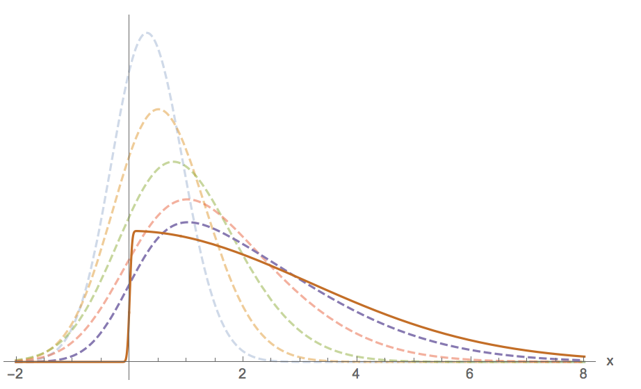
which shows how the $h$-transform constructed in Eq. (11) skews the measure $P$ to the right, and at the final time $T$ limits the achievable states of the diffusion to the state space $x\geq x_{0}$.

2.1.1 Skew-Normal Diffusions

Consider now the BM case, namely $f(x,t)=0$ in Eq.(3), (without loss of generality, we from now on restrict to unit variance):

$$\begin{array}[]{l}dX_{t}=dW_{t},\qquad X_{0}=x_{0},\quad\Rightarrow\quad p_{{\rm BM}}(x,t|x_{0},0)=\frac{e^{-\frac{(x-x_{0})^{2}}{2t}}}{\sqrt{2\pi t}}=\phi\left(\frac{x-x_{0}}{\sqrt{t}}\right),\end{array}$$ (12)

and here the solution of the BFPE and its distribution read:

$$\left\{\begin{array}[]{l}p_{{\rm BM}}[y,T|x,(T-t)]=\frac{e^{-\frac{(x-y)^{2}}{2(T-t)}}}{\sqrt{2\pi(T-t)}},\\ \\ {\cal H}[x,(T-t)|y,T]=\int_{-\infty}^{x}\frac{e^{-\frac{(\xi-y)^{2}}{2(T-t)}}}{\sqrt{2\pi(T-t)}}d\xi=\frac{1}{\sqrt{\pi}}\int_{-\infty}^{\frac{x-y}{\sqrt{2(T-t)}}}e^{z^{2}}dz=\frac{1}{2}\left[1+{\rm Erf}\left(\frac{x-y}{\sqrt{2(T-t)}}\right)\right].\end{array}\right.$$ (13)

From Eqs.(12) and (13), we can establish:

Proposition 1.

For $t\in[0,T]$, the couple of dual Markov diffusion processes solving the SDE:

$$\begin{array}[]{l}dX_{t}=f_{\pm}(X_{t},t)dt+dW_{t},\qquad X_{0}=x_{0},\qquad t\in[0,T],\\ \\ f_{\pm}(x,t):=\partial_{x}\ln{\cal H}_{\pm}(x,T-t)=\partial_{x}\ln\left[\Phi\left(\frac{\pm x}{\sqrt{(T-t)}}\right)\right],\end{array}$$ (14)

are fully characterised by the dual skew-Normal TPDs $p_{\pm}(x,t|x_{0},0)$ given by

$$p_{\pm}(x,t|x_{0},0)=\phi\left(\frac{x-x_{0}}{\sqrt{t}}\right)\left[\frac{\Phi\left(\frac{\pm x}{\sqrt{(T-t)}}\right)}{\Phi\left(\frac{\pm x_{0}}{\sqrt{T}}\right)}\right]=ESK\left(\sqrt{\frac{t}{T-t}},\pm\frac{x_{0}}{\sqrt{t}};\pm\frac{x}{\sqrt{t}}\right),\quad t\in[0,T].$$ (15)

Proof of Proposition 1.

The proposition follows directly from the previous results, Eq. (7) and the definition Eq.(2). Alternatively, the proof can be obtained by direct substitution of Eq.(15) into the FPE:

$$\left\{\begin{array}[]{l}\partial_{t}p_{\pm}(x,t|x_{0},0)={\cal L}[p_{\pm}(x,t|x_{0},0)],\\ \\ {\cal L}[\cdot]:=-\partial_{x}\left\{f_{\pm}(x,t)[\cdot]\right\}+\frac{1}{2}\partial_{xx}[\cdot].\end{array}\right.$$ (16)

$\Box$

Figure 1: Transient of the right-skewed TPD $p_{\pm}(x,t|0,0)$ as given by Eq.(15) for the time horizon $T=10$ and increasing time $t$ from $0.5$ to $T$ (thick red curve). By definition of the the Heaviside step function $\mathbbm{1}(x)$, we have $\lim_{t\rightarrow T}\Phi\left(\frac{\sqrt{2}}{\sqrt{T-t}}\right):=\mathbbm{1}(x)$ thus leading to the half-Normal law (red curve).

Remark 1. For $x_{0}=0$ implying $\Phi(0)=\frac{1}{2}$, the TPD $p_{\pm}(x,t|0,0)$ take the standard SKN form Eq.(1).

$$p_{\pm}(x,t|0,0)=SK\left(\frac{t}{\sqrt{T-t}};\frac{\pm x}{\sqrt{t}}\right),\qquad t\in[0,T].$$ (17)

Note that we have $p_{{\rm BM}}(x,t|x_{0},0)=p_{{\rm BM}}(x-x_{0}),t|0,0)=\phi\left(\frac{x-x_{0}}{\sqrt{t}}\right)$. This translation property does however not hold for the SKN process:

$$ESK\left(\sqrt{\frac{t}{T-t}},\pm\frac{x_{0}}{\sqrt{t}};\pm\frac{x}{\sqrt{t}}\right)\neq SK\left(\frac{t}{\sqrt{T-t}};\frac{\pm(x-x_{0})}{\sqrt{t}}\right).$$ (18)

From Eq.(14), we note that $\left[{\cal H}_{-}(x,T-t)+{\cal H}_{+}(x,T-t)\right]=1$.

Remark 2. The TPD Eq.(15) is defined only for finite time horizon $t\in[0,T]$. One may wonder whether one could construct a SKN process for unrestricted time horizon $t\in\mathbb{R}^{+}$. In Appendix B, this question is briefly addressed using the as $h$-transform involving imaginary error function ${\rm Erfi}(x)$. There one shows that such process exists only on positive state space.

3 Alternative constructions of skew-Normal diffusions

Section 2 shows that SKN diffusion processes result directly from a change of probability of the BM. Here we present a set of alternative interpretations.

3.1 The SKN as a truncated marginal of bi-dimensional Gaussian process

The centred binormal probability law is defined as:

$$\begin{array}[]{l}{\cal N}(x,y)dx\,dy=\frac{1}{2\pi\sigma_{1}\sigma_{2}\sqrt{1-\rho^{2}}}\exp\left\{-\frac{(x/\sigma_{1})^{2}+2\rho(x/\sigma_{1})(y/\sigma_{2})-(y/\sigma_{2})^{2}}{2(1-\rho^{2})}\lx@nobreakspace\right\}dx\,dy,\par\end{array}$$ (19)

with variances $\sigma_{1}^{2}$ and $\sigma_{2}^{2}$ and correlations $\rho\in[-1,+1]$. Define a couple of dual truncated marginals as: $\Pi^{\pm}(x)$ as :

$$\left\{\begin{array}[]{l}\Pi^{\pm}(x)dx:=\left[\int_{\mathbb{R}^{\pm}}{\cal N}(x,y)dy\right]dx=\frac{e^{-(x/\sqrt{2}\sigma_{1})^{2}}}{\sqrt{2\pi\sigma_{1}^{2}}}d\mu_{\pm}(x)=\phi(\frac{x}{\sigma_{1}})d\mu_{\pm}(x)\\ \\ d\mu_{\pm}(x):=\frac{1}{2}\left[1\pm{\rm Erf}\left(\frac{\rho x}{\sqrt{2\sigma_{1}^{2}(1-\rho^{2})}}\right)\right]dx,\end{array}\right.$$ (20)

with $\Pi^{-}(x)+\Pi^{+}(x)=\phi(\frac{x}{\sigma_{1}})$. Focusing on SKN diffusion processes, let us introduce a natural dynamic extension of Eqs.(19) and (20) by writing a bi-dimensional diffusion process $(X_{t},Y_{t})\in\mathbb{R}^{2}$, $t\in\mathbb{R}^{+}$ and

$$X_{t}=W_{1,t}\quad{\rm and}\quad Y_{t}=\sqrt{a(t)}W_{1,t}+\sqrt{b(t)}W_{2,t},\qquad a(t)\geq 0\,\,{\rm and}\,\,b(t)\geq 0,$$ (21)

where $W_{1,t}$ and $W_{2,t}$ are independent standard BM’s and $a(t),b(t)$ time-dependent functions. By definition of the BM, we have:

$$\sigma^{2}_{1}(t)=t\quad\sigma^{2}_{2}(t)=t[a(t)+b(t)]\quad{\rm and}\quad\rho^{2}(t)=a(t)t.$$ (22)

Observe at this point that $a(t)$ cannot be chosen arbitrarily since we must have $\rho^{2}(t)\in[-1,+1]$. From Eqs.(19) and (22), the resulting stochastic process $(X_{t},Y_{t})$ is a Gaussian Markov diffusion on $\mathbb{R}^{2}$ with TOD:

$$\begin{array}[]{l}p(x,y,t|x_{0},y_{0},0)=\frac{1}{2\pi t\sigma_{2}(t)\sqrt{1-\rho^{2}(t)}}\exp\left\{-\frac{[(x-x_{0})^{2}/2t]+2\rho(t)[x-x_{0}/\sqrt{t}][(y-y_{0})/\sigma_{2}(t))]-[(y-y_{0})^{2}/\sigma^{2}_{2}(t))]}{2(1-\rho^{2}(t))}\lx@nobreakspace\right\}dx\,dy,\end{array}$$ (23)

Fix now $x_{0}=y_{0}=0$ and as in Eq.(20), define:

$$\left\{\begin{array}[]{l}\int_{\mathbb{R}}p(x,y,t|0,0,0)dy:=\Pi^{\pm}(x,t)=\frac{e^{-\frac{x^{2}}{2t}}}{2\sqrt{2\pi t}}\left\{1\pm{\rm Erf}\left[Z(t)x\right]\right\}dx=\frac{1}{2}SK\left(\pm\sqrt{2t}Z(t);\frac{x}{\sqrt{t}}\right)dx,\\ \\ Z(t):=\frac{\rho(t)\,}{\sqrt{2t[1-\rho^{2}(t)]}}\quad{\rm with}\quad\rho(t)\in[-1,+1].\end{array}\right.$$ (24)

Let us now study the time evolution of $\Pi^{\pm}(x,t)$.

Proposition 2. Given the correlations $\rho(t)\in[-1,+1]$, the SKN law $\Pi^{\pm}(x,t)$ Eq.(24) solves the parabolic pde:

$$\left\{\begin{array}[]{l}\partial_{t}\Pi^{\pm}(x,t)=-\partial_{x}\left[f^{\pm}_{\psi}(x,t)\Pi^{\pm}(x,t)\right]+\frac{1}{2}\partial_{xx}[\Pi^{\pm}(x,t)],\\ \\ f^{\pm}_{\psi}(x,t):=\psi(t)\partial_{x}\ln\left\{1\pm{\rm Erf}[Z(t)x]\right\}.\end{array}\right.$$ (25)

where $\psi(t)$ is given by:

$$\begin{array}[]{l}\psi(t)=\frac{1}{2}+t\partial_{t}\left[\ln\rho(t)\right].\par\end{array}$$ (26)

Proof of Proposition 2: By direct verification, as detailed in Appendix A.

$\Box$

Remark 3.

The density $\Pi^{\pm}(x,t)=\int_{\mathbb{R}}p(x,y,t|0,0,0)dy$ is a projection (truncation mechanism) of a bi-normal Markov diffusion for the special initial condition $x_{0}=y_{0}=0$. Such a projection mechanism destroys information and so the Markov property of the nominal 2D diffusion process is generally not be preserved for arbitrary $\psi(t)$. In Corollary 2 below, it is shown that the information loss can be exactly balanced by an information gain obtained by an ad-hoc correlation increase between the components of the 2D diffusion Eq.(23).

Corollary 2

For finite time horizon $t\in[0,T]$ and correlations $\rho^{2}(t)=t/T$, Eq.(25) and Eq.(14) are identical. For arbitrary $x_{0}\in\mathbb{R}$, both are solved by $ESK\left(\sqrt{\frac{t}{T-t}},\pm\frac{x_{0}}{\sqrt{t}};\pm\frac{x}{\sqrt{t}}\right)$ which is the TPD characterising a Markov diffusion process.

Proof of Corollary 2: For correlations $\rho^{2}(t)=t/T$, Eq.(26) implies that $\psi(t)=1$. Accordingly the drift component in the pde Eq.(25) coincides with the one in Eq.(14) of Proposition 1. Accordingly, the solution of the corresponding FPE Eq.(16) is given by $ESK\left(\sqrt{\frac{t}{T-t}},\pm\frac{x_{0}}{\sqrt{t}};\pm\frac{x}{\sqrt{t}}\right)$ which fully characterises a Markov diffusion process.

$\Box$

Note that setting $\rho_{t}=\rho\in[0,1)$ (constant correlations, implying $a(t)=\rho,b(t)=\sqrt{1-\rho^{2}},\psi(t)=1/2$), yields a skew-Normal diffusion $X_{t}^{\pm}$ with skewness proportional to $\pm 1/\sqrt{t}$. This specific time-dependence is a suitable feature for stochastic volatility models in finance: for example, multiple empirical studies of the equity skew [27, 28] observe how the S&P 500 short-time skew exhibits the same property as the SKN.

3.2 SKN and dynamic censoring

Assuming $x$ as a centered Gaussian random variable with unit variance and law $\phi(x)$ given in Eq.(1), one defines a couple of one-sided truncated (also referred as censored) probability laws $T_{[a]}(x)$ and $T^{[b]}(x)$ as:

$$\left\{\begin{array}[]{l}T_{[a_{\downarrow}]}(x):={\rm Prob}\left\{x|x>a_{\downarrow}\right\}=\int_{a_{\downarrow}}^{\infty}\phi(x)dx=+\frac{2\phi(x)}{1-{\rm Erf}\left(\frac{a_{\downarrow}}{\sqrt{2}}\right)},\\ \\ T_{[a_{\uparrow}]}(x):={\rm Prob}\left\{x|x<a_{\uparrow}\right\}=\,\int_{-\infty}^{a_{\uparrow}}\phi(x)dx=-\frac{2\phi(x)}{1-{\rm Erf}\left(\frac{a_{\uparrow}}{\sqrt{2}}\right)},\end{array}\right.$$ (27)

Writing $a_{\downarrow}=-(x+\epsilon)$ and $a_{\uparrow}=+(x+\epsilon)$ in Eq.(27) and recalling that ${\rm Erf}\left[-\frac{x}{\sqrt{2}}\right]=-{\rm Erf}\left[\frac{x}{\sqrt{2}}\right]$, we have:

$$\left\{\begin{array}[]{l}\displaystyle\lim_{\epsilon\rightarrow 0}T_{[-(x+\epsilon)]}(x)=+\lim_{\epsilon\rightarrow 0}\left[\frac{2\phi(x)}{1-{\rm Erf}\left(-\frac{x+\epsilon}{\sqrt{2}}\right)}\right]=\sqrt{2}\partial_{x}\ln\left[1+{\rm Erf}\left(\frac{x}{\sqrt{2}}\right)\right],\par\\ \\ \displaystyle\lim_{\epsilon\rightarrow 0}T_{[+(x+\epsilon)]}(x)=-\lim_{\epsilon\rightarrow 0}\left[\frac{2\phi(x)}{1-{\rm Erf}\left(+\frac{x+\epsilon}{\sqrt{2}}\right)}\right]=\sqrt{2}\partial_{x}\ln\left[1-{\rm Erf}\left(\frac{x}{\sqrt{2}}\right)\right].\end{array}\right.$$ (28)

The manifest similarity of Eq.(28) with the drifts terms in Eq.(25) suggests that SKN processes can be understood as an ad-hoc dynamic truncation of a Brownian motion. Indeed, by drawing the increments of a BM from a truncated Gaussian law we can directly generate the SKN drifts. By choosing $a_{\uparrow,(\downarrow)}=\mp Z(t)X_{t}$ in Eq.(28) we directly generate the drifts appearing in Eq.(25). Summarising we have:

Proposition 3: The SKN biases induced by the dual drifts in Eq.(25) are generated by the dynamic censoring of a BM:

$$\left\{\begin{array}[]{l}f_{-}(X_{t},t)=\psi(t)T_{\left[-Z(t)X_{t}\right]}(X_{t}),\\ \\ f_{+}(X_{t},t)=\psi(t)T_{\left[+Z(t)X_{t}\right]}(X_{t}).\end{array}\right.$$ (29)

Proof of Proposition 3 .

The assertion follows directly from Eqs.(25), (27) and (28).

$\Box$

Remark 4:

The characteristic $\frac{\phi(x)}{\Phi(\pm x)}$ structure of the drifts Eq.(25) is typical in reliability theory known as the hazard rate function and in statistics known as the inverse Mills ratio. It naturally arises in the context of the censoring of random variables well known in econometrics [29]. In particular, the relevance of the skew-Normal laws in a static censoring mechanism is well known [30, 31]. Here we have instead a dynamic extension of this mechanism. For all $t\in[0,T]$, the skewness $Z(t)$ increasingly expands the censored part of the domain of $X_{t}$, ultimately leading to a censoring on the half-line $X^{+}_{T}\geq x_{0}$ (respectively $X_{T}^{-}\leq x_{0}$).

4 Properties of the SKN diffusion process

Since the SKN diffusion processes can be derived from a Brownian motion via a change of probability measure, they retain several remarkable properties of the Brownian motion itself.

4.1 Moments of the SKN diffusion process

Corollary 3

The generating function for the moments of the SKN process Eq.(15) reads:

$$G_{\pm}(k,t):=\int_{\mathbb{R}}e^{k(x-x_{0})}ESK\left(\sqrt{\frac{t}{T-t}},\pm\frac{x_{0}}{\sqrt{t}};\pm\frac{x}{\sqrt{t}}\right)dx=\frac{\left[e^{\frac{k^{2}t}{2}}\pm{\rm Erf}\left(\frac{x_{0}-kt}{\sqrt{2T}}\right)\right]}{\left[1\pm{\rm Erf}\left(\frac{x_{0}}{\sqrt{2T}}\right)\right]}.$$ (30)

Proof of Corollary 3

By direct integration, see Appendix C.

$\Box$

The first two moments follow easily by using Eq.(30):

$$\left\{\begin{array}[]{l}\mathbb{E}\left\{(x-x_{0})\right\}=\frac{d}{dk}G_{\pm}(k,t)\mid_{k=0}=tf_{\mp}(x_{0}),\\ \\ \mathbb{E}\left\{(x-x_{0})^{2}\right\}=\frac{d^{2}}{dk^{2}}G_{\pm}(k,t)\mid_{k=0}=t\left[1-\frac{t}{T}x_{0}f_{\mp}(x_{0})\right],\par\end{array}\right.$$ (31)

the latter result showing how SKN processes behave diffusively for $x_{0}=0$ (the variance of the process increases linearly in time), and sub-diffusively [32, 33] as $x_{0}$ increases (for $f_{+}(x_{0})$, viceversa for $f_{-}(x_{0}))$.

4.2 Linear transformations of the ESKN processes

A fundamental property of the Gaussian law is its invariance under linear transformations. This exceptional property is preserved in SKN processes. Let us show this by considering the degenerate 2-D diffusion process n $\mathbb{R}^{2}$:

$$\left\{\begin{array}[]{l}dX_{t}=-\lambda X_{t}dt+dU_{t},\qquad X_{0}=x_{0},\\ \\ dU_{t}=\partial_{u}\ln\left\{1+{\rm Erf}\left[\frac{u}{\sqrt{2(T-t)}}\right]\right\}_{u=U_{t}}dt+dW_{t},\,\,\,U_{0}=0\,\,\,{\rm for}\,\,\,t\in[0,T].\end{array}\right.$$ (32)

Eq.(Appendix D: Invariance under linear transformations) is a linear transformation of the Markov SKN process $U_{t}$. Physically speaking, the process $X_{t}$ Eq.(Appendix D: Invariance under linear transformations) can be seen as a (linear) Ornstein-Uhlenbeck process driven by a SKN noise source $dU_{t}$. The bi-variate Markov process $(X_{t},U_{t})$ is thus completely characterised by its TPD $p(x,u,t|x_{0},0)$ and we have:

Corollary 4

The $X_{t}$-marginal density of the 2D degenerate diffusion process Eq.(Appendix D: Invariance under linear transformations) belongs to the ESKN family and reads:

$$P_{M}(x,t|x_{0},0):=\int_{\mathbb{R}}p(x,u,t|x_{0},0)du=\frac{e^{-\frac{\left(x-x_{0}e^{-\lambda t}\right)^{2}}{2r(t)}}}{\sqrt{2\pi r(t)}}\left\{1+{\rm Erf}\left[\frac{s(t)\left[x-x_{0}e^{-\lambda t}\right]}{\sqrt{2\left[r^{2}(t)T-r(t)s^{2}(t)e^{-4\lambda t}\right]}}\right]\right\},$$ (33)

with $r(t)=\frac{1-e^{-2\lambda t}}{2\lambda}\quad{\rm and}\quad s(t)=\frac{1-e^{-\lambda t}}{\lambda}$.

Proof of Corollary 4

The full calculation is displayed in Appendix D.

$\Box$

From Eq.(33), we straightforwardly have $\displaystyle\lim_{\lambda\rightarrow 0}r(t)=\lim_{\lambda\rightarrow 0}s(t)=t$. So it is immediate to see that in the $\lambda=0$ limit, Eq.(33), reduces to:

$$\lim_{\lambda\rightarrow 0}P_{M}(x,t|x_{0},0)=\frac{e^{-\frac{(x-x_{0})^{2}}{2t}}}{\sqrt{2\pi t}}\left\{1+{\rm Erf}\left[\frac{x-x_{0}}{\sqrt{2(T-t)}}\right]\right\}.$$ (34)

4.3 The BM as the superposition of SKN diffusions

From Proposition 1 and in particular Eq.(15), we can write:

$$\Phi\left[\frac{-x_{0}}{\sqrt{T}}\right]p_{-}(x,t|x_{0})+\Phi\left[\frac{+x_{0}}{\sqrt{T}}\right]p_{-}(x,t|x_{0})=\frac{e^{-\frac{(x-x_{0})^{2}}{2t}}}{\sqrt{2\pi t}}.$$ (35)

Intuitively, Eq.(35) indicates that the BM’s TPD with initial position $x_{0}$ can be represented as a weighted superposition of left- and right skewed extended SKN processes with opposite chiralities. This is an explicit illustration of Markov functions as introduced in the seminal work of L. C. Rogers and J. Pitman [34]. Directly inspired by their Example 2, define a state space ${\cal S}:=\left\{-1,+1\right\}\times\mathbb{R}$ on which evolves a continuous time Markov stochastic process: $\Xi_{t}=({\cal B},X_{t})$ characterised as follows:

• i)   Consider a Bernoulli process ${\cal B}_{t}$ with realisations $\left\{-1,+1\right\}$. At initial time $t=0$, ${\cal B}_{0}$ delivers either the outcome $b_{0}=\left\{-1,+1\right\}$ with respective probabilites $\Phi\left[\frac{\pm x_{0}}{\sqrt{T}}\right]\in[0,1]$.

• ii) For $t>0$, the diffusive component of the process $\Xi_{t}$ is given by :

  $$\left\{\begin{array}[]{l}dX_{t}=[f_{b_{0}}(X_{t},t)]dt+dW_{t},\qquad X_{0}=x_{0},\\ \\ f_{b_{0}}(x,t)=\partial_{x}\ln\left\{1+b_{0}{\rm Erf}\left[\frac{x}{\sqrt{2(T-t)}}\right]\right\},\qquad b_{0}\in\left\{-1+1\right\},\\ \\ \partial_{t}p_{b_{0}}(x_{0},0|x,t)=-\partial_{x}\left[f_{b_{0}}(x,t)p_{b_{0}}(x_{0},0|x,t)\right]+\frac{1}{2}\partial_{xx}p_{b_{0}}(x_{0},0|x,t).\end{array}\right.$$ (36)

  where $f_{b_{0}}(x,t)$ and $p_{b_{0}}(x_{0},0|x,t)=p_{\pm}(x,t|x_{0},0)$ are the drifts respectively the TPDs given in Eq.(15). This shows that the scalar BM initiated at $x_{0}$ results itself from the superposition of a couple of SKN’s with opposite biases. In other words, the BM itself is a lumped version on of the Markov process $\Xi_{t}$ itself evolving on the enlarged probability state ${\cal S}$.

5 Illustration - finite dimensional nonlinear stochastic filtering

In section 4.2 we saw that the SKN are invariant under linear transformations. This offers the exceptional opportunity to derive an exact and explicit solution for a non-linear filtering problem.

Let us briefly recall first the basic problematic of stochastic filtering. The position $X_{t}$ of a stochastic process is monitored by a measurement device itself corrupted by WGN. The objective of stochastic filtering is to construct a real time and optimal (in the mean square sense) estimate $\hat{X}_{t}$ of the actual position $X_{t}$. The utmost engineering relevance of this general problematic still is the source of an abundant literature. Basics references of direct use in the sequel are [35, 36]. The special situation where the system’s dynamic and the monitoring process both are linear is known as the Kalman-Bucy filtering problem (KFP). The KFP can be solved explicitly, since linearity preserves the Gaussian character of the driving noise sources. Accordingly, for the KFP a finite number of estimate moments of are sufficient to fully solve the filtering problem. The SKN invariance under linear transformations discussed in section 4.2, suggests that observing a SKN process via a linear monitoring platform also offers the possibility to solve exactly a 3-parameters non-Gaussian filtering problem ; this is discussed in this section. Start with the general filtering problem (FIP):

$$\left\{\begin{array}[]{l}dX_{t}=f(X_{t},t)dt+dW_{1,t},\quad\,X_{0}=x_{0},\qquad{\rm(system\,\,evolution)},\\ \\ d{\cal Z}_{t}=\omega X_{t}dt+\sigma dW_{2,t},\qquad{\cal Z}_{0}=x_{0},\,\,\qquad{\rm(monitoring\,\,process)},\par\end{array}\right.$$ (37)

where $dW_{1,t}$ and $dW_{2,t}$ stand for independent WGN’s and $\sigma$ is a positive constant noise amplitude. Eq.(37) synthesises a $\sigma dW_{2,t}$ noisy linear observation $\omega X_{t},\,\,\omega>0$ of the system $X_{t}$.The filtering problem (FIP) consists in constructing a probability measure $\varphi(x,t|{\cal Z}_{\tau})$ to estimate $X_{t}$. As it is clear from the notation, the estimate will be based on the full observation history ${\cal Z}_{\tau}$ for $\tau\in[0,t]$. Accordingly, $\varphi(x,t|{\cal Z}_{\tau})$ is itself a random probability measure which characterises $\hat{X}_{t}$ and it is steadily adapted in real time. Numerous distinct estimators are obviously possible and here one focuses on the optimal one. Hence $\varphi(x,t|{\cal Z}_{\tau})$ which minimises the quadric errors:

$$|\hat{e}|^{2}(t):=\int_{\mathbb{R}}|x-\hat{x}|^{2}\varphi(x,t|{\cal Z}_{\tau})dx,$$ (38)

For the FIP defined by Eq.(37), general stochastic filtering theory establishes that $\varphi(x,t|{\cal Z}_{\tau})$ obeys the Kushner-Stratonovich (KS) stochastic pde:

$$\left\{\begin{array}[]{l}d\varphi(x,t|{\cal Z}_{\tau})={\cal L}[\varphi(x,t|{\cal Z}_{\tau})]dt+\frac{\omega}{\sigma^{2}}\left\{x-\mathbb{E}\left[\hat{X}(t)\right]\right\}\left\{d{\cal Z}_{t}-\mathbb{E}\left[\hat{X}(t)\right])\right\}\varphi(x,t|{\cal Z}_{\tau}),\\ \\ {\cal L}[\cdot]=-\partial_{x}\left[f(x)[\cdot]\right]+\frac{1}{2}\partial_{xx}[\cdot],\\ \\ \mathbb{E}\left[\hat{X}(t)\right]:=\int_{\mathbb{R}}x\varphi(x,t|{\cal Z}_{\tau})dx.\end{array}\right.$$ (39)

The KS stochastic pde is intrinsically non-linear since it involves the real time expectation $\hat{x}(t)$. It is remarkable that the un-normalised function $\phi(x,t|Z_{t})$ defined as:

$$\varphi(x,t|{\cal Z}_{\tau}):=\frac{\psi(x,t|{\cal Z}_{t})}{\int_{\mathbb{R}}\psi(x,t|{\cal Z}_{t})dx}.$$ (40)

follows a linear evolution known as the Zakai equation which reads [36]:

$$\left\{\begin{array}[]{l}d\psi(x,t|{\cal Z}_{\tau})={\cal L}[\psi(x,t|{\cal Z}_{\tau})]dt+\frac{\omega x}{\sigma^{2}}[\psi(x,t|{\cal Z}_{\tau})]d{\cal Z}_{t}\qquad\qquad\qquad({\rm Statonovich\,\,interpretation}),\\ \\ d\psi(x,t|{\cal Z}_{\tau})={\cal L}[\psi(x,t|{\cal Z}_{\tau})]dt-\frac{\omega^{2}x^{2}}{2\sigma^{2}}[\psi(x,t|{\cal Z}_{\tau})]dt+\frac{\omega x}{\sigma^{2}}[\psi(x,t|{\cal Z}_{\tau})]d{\cal Z}_{t}\quad({\rm Ito\,\,interpretation}).\end{array}\right.$$ (41)

Apply these FIP concepts for systems $X_{t}$ and $\tilde{X}_{t}$ related via an $h$-transformation. In relation with Eq.(37), consider the FIP with dynamics:

$$\left\{\begin{array}[]{l}d\hat{X}_{t}=\left[f(\hat{X}_{t},t)+\left\{\partial_{x}\ln[H(x,t)]\right\}_{x=\hat{X_{t}}}\right]dt+dW_{1,t},\quad\hat{X}_{0}=x_{0},\\ \\ d{\cal Z}_{t}=\omega\hat{X}_{t}dt+\sigma dW_{2,t},\qquad{\cal Z}_{0}=x_{0}\end{array}\right.$$ (42)

where $\partial_{t}H(x,t)+{\cal L}[H(x,t)]=0$ as introduced in section 2. The modified evolution Eq.(42) leads to the modified Zakai dynamics:

$$\left\{\begin{array}[]{l}d\hat{\psi}(x,t|{\cal Z}_{\tau})=\hat{{\cal L}}[\hat{\psi}(x,t|{\cal Z}_{\tau})]dt+\frac{\omega x}{\sigma^{2}}[\hat{\psi}(x,t|{\cal Z}_{\tau})]d{\cal Z}_{t},\qquad({\rm Statonovich\,\,interpretation}),\\ \\ \hat{{\cal L}}[\cdot]=-\partial_{x}\left\{[f(x,t)+\partial_{x}\ln[H(x,t)][\cdot]\right\}+\frac{1}{2}\partial^{2}_{xx}[\cdot]\end{array}\right.$$ (43)

5.1 SKN and finite-dimensional nonlinear filters

The Kalman-Bucy FIP results when $f(x,t)$ is linear in $x$. In this case the FIP involves a 2D Gaussian diffusion process and $\varphi(x,t|{\cal Z}_{\tau})$ is itself Gaussian and its moments can be explicitly calculated. This is a finite dimensional FIP since the first two moments fully characterised the filter. This situation can be generalised for certain classes of dynamics, an illustration is now exhibited.

Proposition 4. For the BM (i.e. $f(x,t)=0$), the un-normalised Zakai filters $\psi(x,t|{\cal Z}_{\tau})$ and $\hat{\psi}(x,t|{\cal Z}_{\tau})$ in Eqs.(41) and (43) are related as:

$$\hat{\psi}(x,t|{\cal Z}_{\tau})=H(x,t)\psi(x,t|{\cal Z}_{\tau}).$$ (44)

Proof of Proposition 4:

Take $f(x,t)=0$ implying ${\cal L}[\cdot]=\frac{1}{2}\partial_{xx}[\cdot]$ with initial condition $x_{0}=0$ and $\omega=\sigma=1$ in Eqs.(41) and (42) and we obtain:

$$\left\{\begin{array}[]{l}\partial_{t}H(x,t)+\frac{1}{2}\partial_{xx}H(x,t)=0,\\ \\ d\hat{\psi}(x,t|{\cal Z}_{\tau})=-\partial_{x}\left\{\left[\partial_{x}\ln H(x,t)\right]\hat{\psi}(x,t|{\cal Z}_{\tau})\right\}dt+\frac{1}{2}\partial_{xx}[\hat{\psi}(x,t|{\cal Z}_{\tau})]dt+\frac{\omega x}{\sigma^{2}}[\hat{\psi}(x,t|{\cal Z}_{\tau})]d{\cal Z}_{t},\end{array}\right.$$ (45)

Omitting the arguments, write $\hat{\phi}=H\phi$ verify that it solves Eq.(45), namely:

$$\psi\left(dH+\frac{1}{2}\partial_{xx}H\right)-H\left(d\psi-\frac{1}{2}\partial_{xx}\psi-\frac{\omega x}{\sigma^{2}}\psi d{\cal Z}_{t},\right)=0.$$ (46)

$\Box$

When $f(x,t)=0$, Zakai’s Eq.(41) is solved by a Gaussian, (see Example 6.2.10 in [35] and section 3.6 in [36]) and we have:

$$\left\{\begin{array}[]{l}\psi(x,t|{\cal Z}_{\tau})=e^{-\frac{(x-\hat{X}_{t})^{2}}{2S(t)}}\quad{\rm and}\quad\varphi(x,t|{\cal Z}_{\tau})=\frac{e^{-\frac{(x-\hat{X}_{t})^{2}}{2S(t)}}}{\sqrt{2\pi S(t)}}\\ \\ S(t)=\tanh(t)\quad{\rm and}\quad\hat{X}_{t}=\frac{\int_{0}^{t}\sinh(s)d{\cal Z}_{t}}{\cosh(t)}.\par\end{array}\right.$$ (47)

In Eq.(44), identify $H(x,t)={\cal H}(x,T-t)=\Phi\left(\frac{\pm x}{\sqrt{(T-t)}}\right)$ as given by Eq.(14) and the resulting FIP Eq.(42) is finite dimensional. Hence using Eq.(44), we have immediately a couple of FIPs:

$$\left\{\begin{array}[]{l}\hat{\psi}_{\pm}(x,t|{\cal Z}_{\tau})=\psi(x,t|{\cal Z}_{\tau})\Phi\left(\frac{\pm x}{\sqrt{(T-t)}}\right),\qquad\qquad t\in[0,T],\\ \\ \hat{\varphi}_{\pm}(x,t|{\cal Z}_{\tau})=\varphi(x,t|{\cal Z}_{\tau})\frac{\Phi\left(\frac{\pm x}{\sqrt{(T-t)}}\right)}{\Phi\left(\frac{\pm\hat{X}_{t}\sqrt{\tanh(t)}}{\sqrt{\tanh(t)+(T-t)}}\right)},\par\end{array}\right.$$ (48)

where the normalisation factor of $\hat{\varphi}_{\pm}(x,t|{\cal Z}_{\tau})$ follows by using entry 2.7.1-6 of [37]. Eq.(48) is an illustration belonging to the class of finite dimensional filters first discussed by V. E. Benes [38].

Appendix A: Proof of Proposition 2

Adopt the notations:

$$\begin{array}[]{l}\Pi^{\pm}[x,t]=G[1\pm E],\\ \\ G:=\frac{e^{-\frac{x^{2}}{2t}}}{\sqrt{2\pi t}}\quad{\rm and}\quad E:={\rm Erf}[Z(t)x]=\frac{2}{\sqrt{\pi}}\int_{0}^{Z(t)x}e^{-s^{2}}ds,\\ \\ e=\frac{2}{\sqrt{\pi}}e^{-Z^{2}(t)x^{2}}.\end{array}$$ (49)

Writing for short $Z:=Z(t)$, we have:

$$\begin{array}[]{l}\partial_{t}G=\frac{1}{2}\partial_{xx}G,\quad\partial_{x}G=-\frac{x}{t}G\quad\partial_{x}e=-2Z^{2}xe\\ \\ \partial_{t}E=\dot{Z}xe,\quad\partial_{x}E=Ze,\quad\partial_{xx}E=Z\partial_{x}e=-2Z^{3}xe,\\ \\ \end{array}$$ (50)

The pde Eq.(25) is rewritten, (omitting the arguments):

$$\partial_{t}\Pi^{\pm}=-\psi\partial_{x}\left[\frac{\pm Ze}{1\pm E}\Pi^{\pm}\right]+\frac{1}{2}\partial_{xx}\Pi^{\pm}.$$ (51)

Using Eqs.(49) and (50), Eq.(51) reads:

$$\begin{array}[]{l}{\color[rgb]{1,0,0}[\partial_{t}G][1\pm E]}+[\dot{Z}xe]G=-\psi\partial_{x}\left[\pm ZeG\right]+{\color[rgb]{1,0,0}\frac{1}{2}[1\pm E]\partial_{xx}G}\pm Ze\partial_{x}G\mp(Z^{3}xe)G.\end{array}$$ (52)

Since $\partial_{t}G=\frac{1}{2}\partial_{xx}G$, Eq.(52) can finally be rewritten as:

$$\begin{array}[]{l}\dot{Z}=Z\frac{[\psi-1]}{t}+\left[2\psi-1\right]Z^{3}.\end{array}$$ (53)

Introducing $Z^{2}=\frac{\rho^{2}}{2t(1-\rho^{2})}$ into Eq.(53), the assertion Eq.(26) follows.

$\Box$

Appendix B: The ${\rm Erfi}(x)$ change of measure

One may wonder whether it exists a diffusion similar to Eq.(14) but defined for $t\in\mathbb{R}^{+}$. To address this issue, one notes that the imaginary error function ${\rm Erfi}(x)$ might be used, since we have:

$$\left\{\begin{array}[]{l}{\rm Erfi}\left[\frac{x}{\sqrt{2(T+t)}}\right]:=\frac{2}{\sqrt{\pi}}\int_{0}^{\frac{x}{\sqrt{2(T+t)}}}e^{s^{2}}ds=-i{\rm Erf}\left[\frac{ix}{\sqrt{2(T+t)}}\right],\quad i=\sqrt{-1},\\ \\ \partial_{t}\left\{{\rm Erfi}\left[\frac{x}{\sqrt{2(T+t)}}\right]\right\}+\frac{1}{2}\partial_{xx}\left\{{\rm Erfi}\left[\frac{x}{\sqrt{2(T+t)}}\right]\right\}=0.\end{array}\right.$$ (54)

At this stage, let us recall the confluent hypergeometric function identity:

$${\rm Erfi}(x)=\frac{2x}{\sqrt{\pi}}M\left[\frac{1}{2},\frac{3}{2},x^{2}\right]:=\frac{2x}{\sqrt{\pi}}\sum_{n=0}^{\infty}\frac{\Gamma(a+n)\Gamma(b)}{\Gamma(b+n)\Gamma(a)}\frac{x^{2n}}{2n!}\geq 0\,\,\,\,{\rm for}\,\,x\in\mathbb{R}^{+}\$$ (55)

Accordingly for a positive definite, scalar diffusion process $X_{t}\in\mathbb{R}^{+}$ the function ${\rm Erfi}\left[\frac{x}{\sqrt{2(T+t)}}\right]$ can be used as an $h$-transform. Hence instead of Eq.(15), one may tentatively write:

$$\left\{\begin{array}[]{l}\tilde{p}(x_{0},0|x,t):=\frac{e^{-\frac{(x-x_{0})^{2}}{2t}}}{\sqrt{2\pi t}}\left\{\frac{1+{\rm Erfi}\left[\frac{x}{\sqrt{2(t+T)}}\right]}{{1+\rm Erfi}\left[\frac{x_{0}}{\sqrt{2T}}\right]}\right\},\qquad x,t\in\mathbb{R}^{+},\\ \\ \displaystyle\lim_{t\rightarrow 0}\tilde{p}(x_{0},0|x,t)=\delta(x-x_{0}),\qquad T>0.\end{array}\right.$$ (56)

Note that $\tilde{p}(x_{0},0|x,t)$ is well defined only for $T>0$, (since $\displaystyle\lim_{T\rightarrow 0}{\rm Erfi}\left[\frac{x_{0}}{\sqrt{2T}}\right]=\infty$). The Fokker-Planck equation being a continuity equation, $\tilde{p}(x_{0},0|x,t)$ remains normalised for all $t\in\mathbb{R}^{+}$. Accordingly $\tilde{p}(x_{0},0|x,t)$ is a regular TPD of an underlying diffusion process. Recalling that we have:

$${\rm Erfi}(x)\approx e^{x}\frac{1}{2x}\left[1+{\rm const}\frac{1}{x}+...\right]\quad{\rm for}\quad x\rightarrow\infty,$$ (57)

the asymptotic behaviour of $\tilde{p}(x_{0},0|x,t)$ is given by:

$$\tilde{p}_{T}(x_{0},0|x,t)\approx\frac{\sqrt{2(T+t)}}{x}e^{-\frac{Tx^{2}}{2t(t+T)}}\quad{\rm for}\quad x\rightarrow\infty.$$ (58)

Eq.(58) shows that $T>0$ is indeed mandatory to ensure that $\tilde{p}(x_{0},0|x,t)$ is normalisable.

Appendix C: The moments generating function

By direct integration, we have:

$$\begin{array}[]{l}G_{\pm}(k,t):=\int_{\mathbb{R}}e^{k(x-x_{0})}\frac{e^{-\frac{(x-x_{0})^{2}}{2t}}\left[1\pm{\rm Erf}\left(\frac{x}{\sqrt{2(T-t)}}\right)\right]}{\sqrt{2\pi t}\left[1\pm{\rm Erf}\left(\frac{x_{0}}{\sqrt{2T}}\right)\right]}dx=_{z:=\frac{(x-x_{0})}{\sqrt{2t}}}\\ \\ \frac{1}{\sqrt{\pi}\left[1\pm{\rm Erf}\left(\frac{x_{0}}{\sqrt{2T}}\right)\right]}\int_{\mathbb{R}}e^{-z^{2}+k\sqrt{2t}z}\left[1\pm{\rm Erf}\left(\frac{\sqrt{2t}z+x_{0}}{\sqrt{2(T-t)}}\right)\right]dz=_{\omega:=z-\frac{k\sqrt{t}}{\sqrt{2}}}\\ \\ \qquad\qquad\qquad\frac{e^{\frac{k^{2}t}{2}}}{\sqrt{\pi}\left[1\pm{\rm Erf}\left(\frac{x_{0}}{\sqrt{2T}}\right)\right]}\int_{\mathbb{R}}e^{-\omega^{2}}\left[1\pm{\rm Erf}\left(\frac{\sqrt{2t}\omega+x_{0}-kt}{\sqrt{2(T-t)}}\right)\right]d\omega=\\ \\ \qquad\qquad\qquad\qquad\qquad\qquad\qquad\qquad\qquad\qquad\frac{\left[e^{\frac{k^{2}t}{2}}\pm{\rm Erf}\left(\frac{x_{0}-kt}{\sqrt{2T}}\right)\right]}{\left[1\pm{\rm Erf}\left(\frac{x_{0}}{\sqrt{2T}}\right)\right]},\end{array}$$

where the last equality follows from entry 2.7.1-6 (pp. 63) of [37]. Note that we have $G_{\pm}(0,t)=1$ as normalisation requires.

Appendix D: Invariance under linear transformations

Eq.(32) can be rewritten as:

$$\left\{\begin{array}[]{l}dX_{t}=-\lambda X_{t}dt+\partial_{u}\ln\left\{\Phi(u)\right\}_{u=U_{t}}dt+dW_{t}\qquad X_{0}=x_{0},\\ \\ dU_{t}=\partial_{u}\ln\left\{\Phi(u\right\}_{u=U_{t}}dt+dW_{t},\,\,\,U_{0}=0\,\,\,{\rm for}\,\,\,t\in[0,T].\end{array}\right.$$

with $\Phi(u)=1+{\rm Erf}\left[\frac{u}{\sqrt{2(T-t)}}\right]$ and the corresponding FPE reads:

$$\partial_{t}P=\partial_{x}\left\{\left[\lambda x-\frac{\Phi_{u}}{\Phi}\right]P\right\}-\partial_{u}\left\{\left[\frac{\Phi_{u}}{\Phi}\right]P\right\}+\frac{1}{2}\partial_{xx}P+\partial_{xu}P+\frac{1}{2}\partial_{u}P$$ (59)

with the notation $\Phi_{u}:=\partial_{u}\Phi_{u}$ Write $P=\Phi Q$ and Eq.(59) reads:

$$\begin{array}[]{l}Q\Phi_{t}+\Phi Q_{t}=\Phi\partial_{x}\left\{\lambda xQ\right\}-\Phi_{u}Q_{x}-\partial_{u}\left\{\Phi_{u}Q\right\}+\\ \\ \qquad\qquad\qquad\par\frac{1}{2}\Phi Q_{xx}+\Phi_{u}Q_{x}+\Phi Q_{xu}+\frac{\Phi}{2}Q_{uu}+\frac{Q}{2}\Phi_{uu}+\Phi_{u}Q_{u}.\end{array}$$ (60)

After cancelling out $\Phi_{u}Q_{x}$ and developing the term $\partial_{u}\left\{\Phi_{u}Q\right\}$ we have:

$$\begin{array}[]{l}Q\Phi_{t}+\Phi Q_{t}=\phi\partial_{x}\left\{\lambda xQ\right\}-Q\partial_{uu}\phi-\partial_{u}Q\partial_{u}\phi+\\ \\ \qquad\qquad\qquad\par\frac{1}{2}\Phi\partial_{xx}Q+\Phi\partial_{xu}Q+\frac{\Phi}{2}Q_{uu}+\frac{Q}{2}\Phi_{uu}+\Phi_{u}Q_{u}.\end{array}$$ (61)

Cancelling out the term $\Phi_{u}Q_{u}$, factoring by $Q$ the terms $Q\Phi_{t}$, $Q\partial_{uu}\phi$, $\frac{Q}{2}\Phi_{uu}$ and the remaining terms by $\phi$, we get:

$$\begin{array}[]{l}Q\left\{\Phi_{t}+\frac{1}{2}\phi_{uu}\right\}=\Phi\left\{-Q_{t}+\partial_{x}\left\{\lambda xQ\right\}+\frac{1}{2}Q_{xx}+\partial_{xu}Q_{xu}+\frac{1}{2}Q_{uu}.\right\}.\par\end{array}$$ (62)

The left hand side of Eq.(62) cancels out since $\Phi$ solve the backward heat equation. In the right hand side of Eq.(62), the drift term being linear in $x$, $Q$ is necessarily solved by a bi-variate Gaussian probability density and it can be calculated $Q$ explicitly. To this aim, introduce the change of variables:

$$x\mapsto ye^{\lambda t}\Rightarrow\left\{\begin{array}[]{l}\partial_{t}[\cdot]\mapsto\partial_{t}[\cdot]+\lambda e^{\lambda t}\partial_{y}[\cdot],\\ \\ \partial_{x}[\cdot]\mapsto e^{\lambda t}\partial_{y}[\cdot],\\ \\ \partial_{u}[\cdot]\mapsto\partial_{u}[\cdot],\\ \\ Qdx\mapsto Qe^{\lambda t}dy\par\par\end{array}\right.$$ (63)

Introducing Eq.(63) into Eq.(62), we obtain:

$$\partial_{t}Q(y,u,t|y_{0},0,0):=\partial_{t}Q=\frac{e^{2\lambda t}}{2}\phi\partial_{yy}Q+e^{\lambda t}\partial_{yu}Q+\frac{1}{2}\partial_{uu}Q$$ (64)

According to Chandrasekhar [39], (use Eq.(295) in [39] with the identification $\mu_{1}=0$ and $\mu_{2}=-\lambda$ ), we have:

$$\left\{\begin{array}[]{l}Q=\frac{\exp\left\{-\frac{a(t)(y-y_{0})^{2}+2h(t)(y-y_{0})u+b(t)u^{2}}{2\Delta(t)}\right\}}{2\pi\sqrt{\Delta(t)}},\\ \\ a(t):=t,\qquad h(t):=\frac{\left[1-e^{\lambda t}\right]}{\lambda},\qquad b(t):=-\frac{\left[1-e^{2\lambda t}\right]}{2\lambda},\qquad\Delta(t):=ab-h^{2}.\end{array}\right.$$ (65)

Hence we end with:

$$P(y,u,t|y_{0},0,0)=Q\phi=Q\left[1+{\rm Erf}\left(\frac{u}{\sqrt{2(T-t)}}\right)\right]dy$$ (66)

Calculate finally the marginal density $P_{M}(y,t|y_{0},0)$ using entry 2.6.1-6 of [37] to get:

$$P_{M}(y,t|y_{0},0,0)=\int_{\mathbb{R}}P(y,u,t|y_{0},0,0)du=\frac{e^{-\frac{(y-y_{0})^{2}}{2b(t)}}}{\sqrt{2\pi b(t)}}\left\{1+{\rm Erf}\left[\frac{-h(t)(y-y_{0})}{\sqrt{2[b(t)^{2}(T-t)+b(t)\Delta(t)]}}\right]\right\}.$$ (67)

Returning to the nominal variables for $P_{M}(x,t|x_{0},0)$ we obtain Eq.(33).

References

• [1] A. Azzalini (1985) A class of distributions which includes the normal ones. Scandinavian journal of statistics, pp. 171–178. Cited by: §1.
• [2] A. Azzalini (2013) The skew-normal and related families. Vol. 3, Cambridge University Press. Cited by: §1.
• [3] A. Azzalini (2005) The skew-normal distribution and related multivariate families. Scandinavian journal of statistics 32 (2), pp. 159–188. Cited by: §1.
• [4] A. Capitanio, A. Azzalini, and E. Stanghellini (2003) Graphical models for skew-normal variates. Scandinavian Journal of Statistics 30 (1), pp. 129–144. Cited by: §1.
• [5] N. Loperfido and P. Guttorp (2008) Network bias in air quality monitoring design. Environmetrics 19 (7), pp. 661–671. Cited by: §1.
• [6] Y. V. Marchenko and M. G. Genton (2012) A Heckman selection-t model. Journal of the American Statistical Association 107 (497), pp. 304–317. Cited by: §1.
• [7] S. K. Jha and N. V. Singh (2023) A skew-normal spatial simultaneous autoregressive model and its implementation. Sankhya A 85 (1), pp. 306–323. Cited by: §1.
• [8] C. R. Harvey, J. C. Liechty, M. W. Liechty, and P. Müller (2010) Portfolio selection with higher moments. Quantitative Finance 10 (5), pp. 469–485. Cited by: §1.
• [9] J. L. Doob (1957) Conditional brownian motion and the boundary limits of harmonic functions. Bulletin de la Société Mathématique de France 85, pp. 431–458. Cited by: §1.
• [10] H. Kunita (1969) Absolute continuity of markov processes and generators. Nagoya Mathematical Journal 36, pp. 1–26. Cited by: §1.
• [11] K. Ito and S. Watanabe (1965) Transformation of markov processes by multiplicative functionals. Annales de l’institut Fourier 15 (1), pp. 13–30. Cited by: §1.
• [12] W. H. Fleming and S. Sheu (1997) Asymptotics for the principal eigenvalue and eigenfunction of a nearly first-order operator with large potential. The Annals of Probability 25 (4), pp. 1953–1994. Cited by: §1.
• [13] W. H. Fleming (1977) Exit probabilities and optimal stochastic control. Applied Mathematics and Optimization 4, pp. 329–346. Cited by: §1.
• [14] P. Dai Pra (1991) A stochastic control approach to reciprocal diffusion processes. Applied mathematics and Optimization 23 (1), pp. 313–329. Cited by: §1.
• [15] L. C. G. Rogers and D. Williams (2000) Diffusions, markov processes and martingales: volume 2, itô calculus. Vol. 2, Cambridge university press. Cited by: §1.
• [16] R. Chetrite and H. Touchette (2015) Nonequilibrium markov processes conditioned on large deviations. Annales Henri Poincaré 16 (9), pp. 2005–2057. Cited by: §1.
• [17] K. Itô and H. McKean (1963) Brownian motions on a half line. Illinois journal of mathematics 7 (2), pp. 181–231. Cited by: §1.
• [18] J. M. Harrison and L. A. Shepp (1981) On skew brownian motion. The Annals of probability, pp. 309–313. Cited by: §1.
• [19] Y. Ouknine (1991) “Skew-brownian motion” and derived processes. Theory of Probability & Its Applications 35 (1), pp. 163–169. Cited by: §1.
• [20] A. Lejay (2006) On the constructions of the skew brownian motion. Probability Surveys 3, pp. 413–466. Cited by: §1.
• [21] T. Appuhamillage, V. Bokil, E. Thomann, E. Waymire, and B. Wood (2011) Occupation and local times for skew brownian motion with applications to dispersion across an interface. The Annals of Applied Probability 21 (1), pp. 183–214. Cited by: §1.
• [22] M. Decamps, A. De Schepper, and M. Goovaerts (2004) Applications of δ\delta-function perturbation to the pricing of derivative securities. Physica A: Statistical Mechanics and its Applications 342 (3-4), pp. 677–692. Cited by: §1.
• [23] A. Gairat and V. Shcherbakov (2017) Density of skew brownian motion and its functionals with application in finance. Mathematical Finance 27 (4), pp. 1069–1088. Cited by: §1.
• [24] P. C. Bressloff (2022) A probabilistic model of diffusion through a semi-permeable barrier. Proceedings of the Royal Society A 478 (2268), pp. 20220615. Cited by: §1.
• [25] A. Borodin and P. Salminen (2002) Handbook of brownian motion - facts and formulae. Birkhäuser. Cited by: §2, §2.
• [26] C. Gardiner (2010) Stochastic methods-a handbook for the natural and social sciences. Springer. Cited by: §2.1, §2.
• [27] P. Carr and L. Wu (2003) The finite moment log stable process and option pricing. The journal of finance 58 (2), pp. 753–777. Cited by: §3.1.
• [28] M. Azzone and R. Baviera (2022) Additive normal tempered stable processes for equity derivatives and power-law scaling. Quantitative Finance 22 (3), pp. 501–518. Cited by: §3.1.
• [29] F. Hayashi (2011) Econometrics. Princeton University Press. Cited by: §3.2.
• [30] J. J. Heckman (1979) Sample selection bias as a specification error. Econometrica, pp. 153–161. Cited by: §3.2.
• [31] A. Azzalini, H. Kim, and H. Kim (2019) Sample selection models for discrete and other non-gaussian response variables. Statistical Methods & Applications 28 (1), pp. 27–56. Cited by: §3.2.
• [32] S. B. Alves, G. F. de Oliveira Jr, L. C. de Oliveira, T. P. de Silans, M. Chevrollier, M. Oriá, and H. L. d. S. Cavalcante (2016) Characterization of diffusion processes: normal and anomalous regimes. Physica A: Statistical Mechanics and its Applications 447, pp. 392–401. Cited by: §4.1.
• [33] P. Massignan, C. Manzo, J. A. Torreno-Pina, M. F. García-Parajo, M. Lewenstein, and G. J. Lapeyre Jr (2014) Nonergodic subdiffusion from brownian motion in an inhomogeneous medium. Physical review letters 112 (15), pp. 150603. Cited by: §4.1.
• [34] L. C. Rogers and J. Pitman (1981) Markov functions. The Annals of Probability, pp. 573–582. Cited by: §4.3.
• [35] B. Oksendal (1998) Stochastic differential equations - an introduction with applications. Springer. Cited by: §5.1, §5.
• [36] Z. Schuss (2012) Nonlinear filtering and optimal phase tracking. Springer. Cited by: §5.1, §5, §5.
• [37] N. E. Korotkov and A. N. Korotkov (2020) Integrals related to the error function. CRC Press. Cited by: §5.1, Appendix C: The moments generating function, Appendix D: Invariance under linear transformations.
• [38] V. Benes (1981) Exact finite dimensional filters for certain diffusions with nonlinear drift. Stochastics 5 (1-2), pp. 65–92. Cited by: §5.1.
• [39] S. Chandrasekhar (1943) Stochastic problems in physics and astronomy. Review of Modern Physics 15 (1), pp. 1–88. Cited by: Appendix D: Invariance under linear transformations.