Perpetual maintenance of machines with different urgency requirements Thanks: L. Gąsieniec and J. Min’s work was partially supported by Network Sciences and Technologies (NeST) at University of Liverpool. This study has been carried out in the frame of “the Investments for the future” Programme IdEx Bordeaux – SysNum (ANR-10-IDEX-03-02). R. Klasing’s research was partially supported by the ANR project TEMPOGRAL (ANR-22-CE48-0001). C. Levcopoulos and A. Lingas work were supported by the Swedish Research Council grants 621-2017-03750 and 2018-04001. T. Radzik’s work was supported in part by EPSRC grant EP/M005038/1, “Randomized algorithms for computer networks.” Part of this work was done while T. Radzik was visiting the LaBRI as a guest professor of the University of Bordeaux. T. Jurdzinski’s work was supported by the Polish National Science Centre project no. 2020/39/B/ST6/03288. Preliminary versions of some of the results presented in this paper appeared in Proc. 43rd International Conference on Current Trends in Theory and Practice of Computer Science (SOFSEM 2017), LNCS 10139, pp. 229–240, Springer (2017) [25].

Abstract

A garden $G$ is populated by $n\geq 1$ bamboos $b_{1},b_{2},...,b_{n}$ with the respective daily growth rates $h_{1}\geq h_{2}\geq\dots\geq h_{n}$. It is assumed that the initial heights of bamboos are zero. The robotic gardener maintaining the garden regularly attends bamboos and trims them to height zero according to some schedule. The Bamboo Garden Trimming Problem (BGT) is to design a perpetual schedule of cuts to maintain the elevation of the bamboo garden as low as possible. The bamboo garden is a metaphor for a collection of machines which have to be serviced, with different frequencies, by a robot which can service only one machine at a time. The objective is to design a perpetual schedule of servicing which minimizes the maximum (weighted) waiting time for servicing.

We consider two variants of BGT. In discrete BGT the robot trims only one bamboo at the end of each day. In continuous BGT the bamboos can be cut at any time, however, the robot needs time to move from one bamboo to the next.

For discrete BGT, we show tighter approximation algorithms for the case when the growth rates are balanced and for the general case. The former algorithm settles one of the conjectures about the Pinwheel problem. The general approximation algorithm improves on the previous best approximation ratio. For continuous BGT, we propose approximation algorithms which achieve approximation ratios $O(\log\lceil h_{1}/h_{n}\rceil)$ and $O(\log n)$.

Key Words: Bamboo Garden Trimming problem, BGT problem, Perpetual scheduling, Periodic maintenance, Pinwheel scheduling, Approximation algorithms, Patrolling

1 Introduction

We consider a perpetual scheduling problem in which $n\geq 2$ (possibly virtual) machines need to be attended (serviced) with known but possibly different frequencies, i.e. some machines need to be attended more often than others. The frequencies of attending individual machines are specified as positive weights $h_{1},h_{2},\dots,h_{n}$ and the objective is to design a perpetual schedule of attending the machines which minimizes the maximum weighted time any individual machine waits for the next service. Since a higher weight $h_{i}$ (comparing with other weights) means that machine $i$ should be attended relatively more frequently, we refer to the weights also as urgency factors. The same optimization problem arises when a data stream keeps filling a collection of $n$ buffers according to a known distribution: buffer $i$ receives $h_{i}$ units of data in each unit of time. The objective is to design a perpetual schedule of emptying the buffers which minimizes the maximum occupancy of any individual buffer.

We model such perpetual scheduling problems using the following metaphor of the Bamboo Garden Trimming (BGT) Problem. A collection (garden) of $n\geq 2$ bamboos $b_{1},b_{2},\ldots,b_{n}$ with known respective daily growth rates $h_{1},h_{2},\dots,h_{n}$. We assume that these growth rates are already arranged into a non-increasing sequence: $h_{1}\geq h_{2}\geq\dots\geq h_{n}>0$. Initially the height of each bamboo is set to zero. The robotic gardener maintaining the garden trims bamboos to height zero according to some schedule. The height of a bamboo $b_{i}$ at time $t\geq 0$ is equal to $(t-t^{\prime})h_{i}$, where $t^{\prime}$ is the last time when this bamboo was trimmed, or $t^{\prime}=0$, if it has never been trimmed by time $t$. The main task of the BGT problem is to design a perpetual schedule of cuts to keep the highest bamboo in the garden as low as possible, while complying with some specified constraints on the timing of cutting. The basic constraints considered in this paper are that the gardener can cut only one (arbitrary) bamboo at the end of each day and is not allowed to attend the garden at any other times. Once the gardener has decided which bamboo to trim in the current round (at the end of the current day), then the action of actual trimming is instantaneous.

Referring back to the two scheduling problems mentioned earlier, the heights of the growing bamboos would represent the weighted times the machines wait for the next service, or the current occupancy of the data buffers. The action of cutting a bamboo $b_{i}$ at the end of the current day represents attending machine $i$ or emptying buffer $i$ in the current time slot. Other problems which can be modeled by BGT include the perpetual testing of virtual machines in cloud systems [1]. In such systems frequency in which virtual machines are tested for undesirable symptoms vary depending on the importance of dedicated cloud operational mechanisms.

We consider two variants of the BGT problem. The constraint that only one bamboo is cut at the end of each day (round) defines discrete BGT. The gardener has equal access to all bamboos, so can select in each round any bamboo for cutting. In the second variant, continuous BGT, we assume that for any two bamboos $b_{i}$ and $b_{j}$, we know the time $t_{i,j}>0$ (which may be fractional) that the robot needs to relocate from $b_{i}$ to $b_{j}$. In this variant the time when the next bamboo is trimmed depends on how far that bamboo is from the bamboo which has just been trimmed. As in discrete BGT, when the robot arrives at the bamboo to trim it, the actual action of trimming is instantaneous. In this paper we consider symmetric travel times (that is, $t_{i,j}=t_{j,i}$) and assume that the robot travels always along the fastest route, so the travel times satisfy the triangle inequality. We also assume that the robot is initially at the location of $b_{1}$. Discrete BGT is the special case of continuous BGT when all travel times $t_{i,j}$, for $i\neq j$, are the same, while metric TSP is the special case of continuous BGT when all growth rates $h_{i}$ are the same.

In both discrete and continuous cases, we consider algorithms ${\cal{A}}$ which for an input instance $I$ of the form $(h_{i}:\>1\leq i\leq n)$ in the discrete case and $[(h_{i}:\>1\leq i\leq n)$, $(t_{i,j}:\>1\leq i,j\leq n)]$ in the continuous case, produce a perpetual (trimming) schedule ${\cal{A}}(I)$ as a sequence of indices of bamboos $(i_{1},i_{2},\ldots)$ which defines the order in which the bamboos are trimmed. We are mainly interested in the approximation ratios of such algorithms, which are defined in the usual way. For an input instance $I$ and a trimming schedule ${\cal{S}}$ for $I$, let ${\mbox{\it MH}}({\cal{S}})$ denote the supremum of the heights of bamboos over all times $t\geq 0$ when the trimming proceeds according to schedule ${\cal{S}}$, and let ${\mbox{\it OPT}}(I)$ denote the infimum of ${\mbox{\it MH}}({\cal{S}})$ over all schedules ${\cal{S}}$ for $I$. The approximation ratio of a schedule ${\cal{S}}$ is defined as ${\mbox{\it MH}}({\cal{S}})/{\mbox{\it OPT}}(I)$ and the approximation ratio of an algorithm ${\cal{A}}$ is the supremum of ${\mbox{\it MH}}({\cal{A}}(I))/{\mbox{\it OPT}}(I)$ over all input instances $I$.

Regarding the time complexity of BGT algorithms, we aim at polynomial preprocessing time followed by computation of the consecutive indices of the schedule in poly-logarithmic time per one index. We will call algorithms with such performance simply polynomial-time (BGT) algorithms. The computational complexity of continuous BGT is related to the complexity of TSP, as the latter is a special case of the former. To discuss computational complexity of discrete BGT, we introduce first a lower bound on the height of schedules.

For each instance $I$ of discrete BGT with the sum of the growth rates $H=H(I)=h_{1}+h_{2}+\dots+h_{n}$, a simple and natural lower bound on the maximum height of a bamboo in any schedule is ${\mbox{\it OPT}}(I)\geq H$. Indeed, while the heights of all bamboos are at most $H^{\prime}<H$, then during each day the total height of all bamboos, that is, the sum of the current heights of all bamboos, increases at least by $H-H^{\prime}>0$ (the total growth over all bamboos is $H$ but only one bamboo, of height at most $H^{\prime}$, is cut). Thus on some day within the first $\lfloor nH^{\prime}/(H-H^{\prime})\rfloor+1$ days the total height of the bamboos must exceed $nH^{\prime}$, so the height of one of the bamboos must exceed $H^{\prime}$. Observe also that it cannot happen that the maximum height of a bamboo approaches $H$ but never reaches $H$, because there are only finitely many possible heights of bamboos which are less than $H$.

There are instances with ${\mbox{\it OPT}}(I)=H$. The obvious one is the uniform instance $h_{i}\equiv H/n$. A non-uniform example is the input instance $I=(1/2,1/4,1/4)$, where all bamboos are kept within the $H=1$ height by the schedule with period $(b_{1},b_{2},b_{1},b_{3})$. An example of an input instance with ${\mbox{\it OPT}}(I)>H$ is $I=(7/15,1/3,1/5)$, for which $H=1$ but ${\mbox{\it OPT}}(I)=4/3$. For this instance, the schedule with period $(b_{1},b_{2},b_{1},b_{2},b_{1},b_{3})$ does not let any bamboo grow above the height $4/3$. On the other hand, a schedule which keeps the heights of $b_{1}$ and $b_{2}$ strictly lower than $4/3$ must cut $b_{1}$ every other day, implying that $b_{2}$ must also be cut every other day (after the initial couple of days). Thus, after the initial couple of days, there are no further days available to cut $b_{3}$, so its height grows to infinity. If we have only two bamboos and their growth rates are $h_{1}=1-\varepsilon$, and $h_{2}=\varepsilon$, for any $0<\varepsilon\leq 1/2$, then ${\mbox{\it OPT}}(I)=2(1-\varepsilon)$, so can be arbitrarily close to $2$. We note here that for any instance $I$, ${\mbox{\it OPT}}(I)\leq 2H(I)$ (this is explained in Section 4.1).

The context and previous related research

Our paper focuses on perpetual maintenance of a given environment where each vital element has its own, possibly unique urgency factor. This makes it related to periodic scheduling [38], a series of papers on the Pinwheel problems [13, 14, 26] including the periodic Pinwheel problem [27, 35] and the Pinwheel scheduling problem [37], as well as the concept of P-fairness in sharing multiple copies of some resource among various tasks [5, 6].

The Pinwheel problem introduced in [26] can be viewed as a special case of discrete BGT. The complexity results for the Pinwheel problem presented in [26] imply that for a given $K\geq H$, if there is a schedule with height at most $K$, then there is a cyclic schedule with height at most $K$, but the shortest such schedule can have exponential length. This implies that the decision version of discrete BGT can be solved by considering all cyclic schedules of up to exponential length, and this can be implemented in PSPACE. Further from [26], while the cyclic schedules of height $H$ can also have exponential length, they have concise polynomial-size representations, and there is a polynomial-time algorithm for checking if a given concise representation of a cyclic schedule of height $H$ is valid. This implies that the restricted decision version of discrete BGT which asks if there is a schedule of height $H$ is in NP. Jacobs and Longo [28] show that there is no pseudopolynomial time algorithm solving the Pinwheel problem unless SAT has an exact algorithm running in expected time $n^{O(\log n\log\log n)}$ and consider the complexity of related problems. However, the exact complexity of the Pinwheel problem remains a long-standing open question.

In related research on minimizing the maximum occupancy of a buffer in a system of $n$ buffers, the usual setting is a game between the player and the adversary [8, 11, 16]. The adversary decides how the fixed total increase of data in each round is distributed among the buffers and tries to maximize the maximum occupancy of a buffer. The player decides which buffer (or buffers, depending on the variant of the problem) should be emptied next and tries to minimize the maximum buffer size. The upper bounds developed in this more general context can be translated into upper bounds for our BGT problems, but our aim is to derive tighter bounds for the case when the rates of growth of the occupancy of buffers, or the rates of growth of bamboos in our terminology, are fixed and known. Similar models, under the name of “cup (emptying) games”, have been considered, with recent papers including [7, 9, 32, 33, 34].

The continuous BGT problem is a natural extension of several classical algorithmic problems with the focus on monitoring and mobility, including the Art Gallery Problem [15] and its dynamic extension called the $k$-Watchmen Problem [39]. In a more recent work on fence patrolling [18, 19, 30] the studies focus on monitoring vital (possibly disconnected) parts of a linear environment where each point is expected to be attended with the same frequency. Czyzowicz et al. [20] study monitoring linear environments by robots prone to faults. Problems similar to continuous BGT are considered also by Baller et al. [4], who focus on special cases (special metric spaces) to investigate the boundary between easy (that is, polynomial) and hard cases, and by Bosman et al. [12], who minimize the travel cost subject to the feasibility requirement of maintaining the specified minimum frequencies of visiting bamboos.

Probably the most natural strategy to keep the elevation of the bamboo garden low is the greedy approach of always moving next to the currently highest bamboo and cutting it. This approach, called Reduce-Max, is particularly appealing in the context of discrete BGT, where there are no travel times to be accounted for. Reduce-Max was considered recently in the context of periodic testing of virtual machines in cloud systems [1], and was also studied in the adversarial setting of the buffer minimization problems mentioned above. The results presented in [11] imply a tight upper bound of $H\cdot(H_{n-1}+1)=\Theta(H\log n)$ on ${\mbox{\it MH}}({\cal{S}})$ for schedules ${\cal{S}}$ produced by Reduce-Max for a variant of the discrete BGT with the adversary which in each round arbitrarily distributes the total daily growth of $H$ among the bamboos. Here $H_{k}=\sum_{i=1}^{k}\frac{1}{k}=\Theta(\log k)$ is the $k$-th harmonic number. While this $O(H\log n)$ upper bound applies obviously also to our non-adversarial discrete BGT, when the growth rates are fixed, it was a long standing open question whether there were instances for which Reduce-Max lets some bamboos grow to heights $\Omega(H\log n)$, or even to heights $\omega(H)$. The experimental work presented in [1] pointed towards a conjecture that Reduce-Max keeps the maximum bamboo height within $O(H)$, and the question has been finally recently answered in Bilò et al. [10], where a bound of $9H$ on the maximum bamboo height under the Reduce-Max algorithm was proven. Kuszmaul [31] has recently shown that the maximum height of a bamboo under the Reduce-Max cutting strategy is at most $4H$.

As mentioned above, there are instances for which the optimal maximum height can be arbitrarily close to $2H$ (see also Bilò et al. [10] and Kuszmaul [31]). This, however, does not imply a lower bound greater than $1$ on the approximation ratio of any algorithm (which is defined with respect to the optimum rather than the lower bound $H$). We note that the input instance $I=(3/8-\varepsilon,1/4,1/4)$, where $0<\varepsilon<1/24$ can be arbitrarily small, shows that the approximation ratio of Reduce-Max cannot be less than $9/8$. For this instance, ${\mbox{\it OPT}}(I)=1$ (for $\varepsilon<1/24$) with the optimal schedule repeating $(b_{1},b_{2},b_{1},b_{3})$, but the Reduce-Max schedule is $(b_{1},b_{2},b_{3},b_{1},\ldots)$, with the first bamboo reaching the height $9/8-3\varepsilon$. In Section 2 we show that the approximation ratio of Reduce-Max is not less than $12/7$.

In [25], which included preliminary versions of some of the results presented in this paper, we introduced a modification of Reduce-Max, which we called Reduce-Fastest, to show the first simple greedy algorithm achieving constant approximation ratio. $\mbox{Reduce-Fastest}(x)$, where $x>0$ is a parameter of the algorithm, works in the following way. Keep track of the “tall” bamboos, defined as having the current height at least $x\cdot H$, and cut in each step the tall bamboo with the highest growth rate (no cutting, if there is no tall bamboo). In [25], we presented a detailed proof that the approximation ratio of $\mbox{Reduce-Fastest}(2)$ is at most $4$. D’Emidio et al. [23] conducted an extensive experimental evaluation of various BGT strategies, which led them to conjecture that Reduce-Max, $\mbox{Reduce-Fastest}(2)$, and $\mbox{Reduce-Fastest}(1)$ keep the maximum height of a bamboo within $2H$, $3H$, and $2H$, respectively. Subsequently, Bilò et al. [10] proved that for $x=1+1/\sqrt{5}\approx 1.45$, the maximum bamboo height under the $\mbox{Reduce-Fastest}(x)$ strategy is not greater than an approximation ratio of $(3+\sqrt{5})/2\approx 2.62$. They also presented efficient implementations of Reduce-Fastest and Reduce-Max.

Kuszmaul [31] has recently shown that for any $x\geq 2$, the strategy $\mbox{Reduce-Fastest}(x)$ keeps all bamboos strictly below $(x+1)\cdot H$, proving this way the conjecture from [23] that $\mbox{Reduce-Fastest}(2)$ keeps the bamboos below $3H$. For a lower bound, Kuszmaul [31] has shown that whatever the value of parameter $x$ is, $\mbox{Reduce-Fastest}(x)$ does not give a bound better than $(2.01)\cdot H$, disproving the conjecture from [23] that $\mbox{Reduce-Fastest}(1)$ keeps bamboos below $2H$. The lower bound of $(2.01)\cdot H$ together with the bound ${\mbox{\it OPT}}(I)\leq 2H(I)$ imply that the approximation ratio of Reduce-Fastest is at least $2.01/2=1.005$. In Section 2, we give examples showing better lower bounds on the approximation ratio of Reduce-Fastest. Bilò et al. [10] and Kuszmaul [31] consider algorithms which guarantee the $2H$ bound on the maximum bamboo height (the best possible bound with respect to $H$), the former focusing on resource-efficient algorithms and the latter on simplicity of computation. These algorithms therefore have approximation ratios at most $2$, but it is not known if those ratios are strictly less than $2$.

We refer informally to BGT algorithms like Reduce-Max and Reduce-Fastest as online scheduling. These algorithms are based on simple greedy strategies, the trimming schedule is revealed while the cutting progresses, and the whole cutting process would naturally adapt to changing growth rates. An alternative offline scheduling pre-computes the whole (cyclic) schedule. This approach would sacrifice the flexibility offered by simple greedy strategies but hopefully would give better approximation ratios. Indeed, using the Pinwheel results given in [26], one can easily obtain an offline algorithm ${\cal{A}}$ which guarantees ${\mbox{\it MH}}({\cal{A}}(I))\leq 2H(I)$ for each input $I$, so a $2$-approximation algorithm for discrete BGT. An efficient implementation of this algorithm was developed in [10]. Recently, [40] has shown an offline scheduling algorithm, also based on Pinwheel results, which guarantees $12/7$-approximation – the best approximation ratio for the general problem shown prior to our paper. We emphasise that our online/offline categorisation of scheduling algorithms is informal, and does not refer to the availability of input (in both cases the whole input is known in advance) but only indicates the general nature of algorithms. Similarly, to distinguish algorithms like Reduce-Max and Reduce-Fastest from more complex approaches, Kuszmaul [31] refers informally to this type of algorithms as simple algorithms.

The optimisation objective in our work, and in the related work discussed above, is minimizing the maximum (weighted) waiting time (the maximum height of a bamboo). Anily et al. [2, 3] consider perpetual scheduling of servicing machines with the objective of minimizing the average (weighted) time of waiting for maintenance (using different but equivalent terminology of ’linearly increasing operational costs’). They show that there is always an optimal schedule which is cyclic and propose and evaluate various strategies of computing schedules for the general case of $n$ machines [2] and for the special case of $3$ machines [3].

Structure of the paper and our contributions

In Sections 2 to 5, we consider the discrete BGT. In Section 2, we derive some lower bounds on the approximation ratios of the simple strategies Reduce-Max and Reduce-Fastest. In Section 3, we elaborate on the Pinwheel problem and its relation to discrete BGT, laying foundations for our main results. In Section 4, we present our main approximation algorithm for discrete BGT, which is an offline algorithm derived by further exploration of the relation between discrete BGT and the Pinwheel problem and has approximation ratio $(1+O(\sqrt{h_{1}/H}))$. The benefits of the relation between the discrete BGT and Pinwheel problems extend both ways. On the one hand, our approximation algorithm uses properties of the Pinwheel problem. On the other hand, the approximation ratio which we achieve settles one of the conjectures about the Pinwheel problem as explained in Section 3.

In Section 5, we turn our attention to general approximation bounds. As mentioned earlier, the best previous general bound is $12/7$ given in [40]. We show an algorithm with approximation ratio $8/5+o(1)<12/7$. This improvement is based on a new approach of splitting the growth rates into two groups of large and small rates, computing good schedules separately for each group, and then merging these two schedules into one schedule for all rates. The algorithm uses the $(1+O(\sqrt{h_{1}/H}))$-approximation algorithm to compute a schedule for the group of small rates.

In Section 6, we show algorithms for continuous BGT with approximation ratios $O(\log\lceil{h_{1}}/{h_{n}}\rceil)$ and $O(\log n)$. We also discuss how tight these approximation ratios are. We show instances of continuous BGT such that for any schedule the maximum bamboo height is greater by a $\Theta(\log n)$ factor than the lower bounds which we use in the analysis of approximation ratios. Thus for these input instances our $O(\log n)$-approximation algorithm computes in fact schedules with constant approximation ratios. We also show instances for which this algorithm computes $\Theta(\log n)$-approximate schedules.

2 Approximation ratio of simple strategies

In Section 1, we presented the previous work on the simple strategies Reduce-Max and Reduce-Fastest, which focused on analysing the maximum height of any bamboo in relation to the sum of the growth rates $H$. The value $H$ is, however, only a lower bound on the optimum, so the bounds in relation to $H$ do not necessarily give good bounds on the approximation ratios, which refer to the optimal values. Recall that there are BGT instances for which the optimal (minimal) height is arbitrarily close to $2H$. In this section, we show some lower bounds on the approximation ratios of these two strategies.

Approximation ratio of Reduce-Max.

 

We show that the approximation ratio of Reduce-Max is not less than $12/7$ by considering the following BGT instances. Let $i=7k+3$, for any integer $k\geq 1$. We have a sequence of $i+1=7k+4$ growth rates partitioned into two groups. In group 1, we have only the largest growth rate $h_{1}=\frac{3k}{i}=3/7-\frac{9}{7i}$, while the remaining $i$ growth rates belong to group 2 and are all equal to $\frac{1}{2i}\/.$ It is easy to see that the optimal (minimal) height for these instances is at most $1$: schedule $b_{1}$ every other time slot and the other bamboos in the remaining slots in the round-robin manner.

We now look at the computation of Reduce-Max on this sequence of growths and consider three initial stages defined as follows.

• Stage 1: all bamboos in group 2 are smaller than $h_{1},$ so $b_{1}$ is cut during each round.

• Stage 2: all bamboos in group 2 are smaller than $2h_{1}$, but some of them are taller than $h_{1}$, implying that $b_{1}$ is cut in every other round, whenever it reaches height $2h_{1}$.

• Stage 3: all bamboos in group 2 are smaller than $3h_{1}$, but some of them are taller than $2h_{1}$, implying that $b_{1}$ is cut in every third round, whenever it reaches height $3h_{1}$.

The main idea is to show not only that Stage 3 is not empty, but also that at the end of Stage 3, there are still 3 bamboos in group 2 which have never been cut. Such bamboos are taller than $3h_{1}$, so $b_{1}$ is not cut for 3 consecutive rounds, growing to the height $4h_{1}$.

In Stage 1 no bamboos from group 2 are cut, and they all grow to height $h_{1},$ at the end of Stage 2, some bamboos from group 2 grow to height $2h_{1}$, and at the end of Stage 3 some bamboos from group 2 grow to height $3h_{1}.$ As in Stage 2 and Stage 3 some bamboos from group 2 are cut, we need to show that we have enough bamboos in this group for some of them not to be cut in either of the three stages.

For each Stage $j$, $j=1,2,3$, there is a bamboo in group 2 which adds $h_{1}$ to its height (growing from $(j-1)h_{1}$ to $jh_{1}$), so there are ${h_{1}}/{\frac{1}{2i}}=h_{1}\cdot 2i=6k$ rounds in every stage. Thus $3k$ bamboos from group 2 are cut in Stage 2 (one group-2 bamboo cut in every other round in this stage), and $4k$ bamboos from group 2 are cut in Stage 3 (two of them are cut in each sequence of 3 consecutive rounds in this stage). Thus, after all three stages, at most $7k$ different bamboos from group 2 will be cut altogether. Hence, at least 3 bamboos from group 2 will not be cut in either of the three stages. 3 of these bamboos will be cut in the next 3 rounds. Therefore, bamboo $b_{1}$ will grow to height $4h_{1}=12/7-o(1)$.

While Reduce-Max pushes the maximum bamboo height close to $12/7$ for our BGT instances, this may be happening only in the initial period of the schedule. However, it is easy to see that in these instances $b_{1}$ will have to keep growing to the height of $3h_{1}$, even in the long run. Otherwise, after some round $t$, the height of each bamboo would never go above $2h_{1}+o(1)<H$, which is not sustainable. Thus, denoting by $m_{t}$ the maximum height of any bamboo at any round after round $t$, our input instances show that we can get $m_{t}\geq 9/7-\varepsilon$, for arbitrarily small $\varepsilon>0$.

Approximation ratio of Reduce-Fastest.

 

For $0<x<1$, the input instance $I=(x,\varepsilon)$, where $0<\varepsilon<\min\{x,1-x\}$, shows that the approximation ratio of $\mbox{Reduce-Fastest}(x)$ is unbounded, as noted in Kuszmaul [31]. For this instance, ${\mbox{\it OPT}}(I)=2x$ with the optimal schedule repeating $(b_{1},b_{2})$, but the $\mbox{Reduce-Fastest}(x)$ schedule never cuts bamboo $b_{2}$, hence the height of bamboo $b_{2}$ grows to infinity.

For $1\leq x<2$, the input instance $I=(x/2-\varepsilon,\varepsilon)$, where $0<\varepsilon<x/2$, shows that the approximation ratio of $\mbox{Reduce-Fastest}(x)$ cannot be less than $3/2$. For this instance, ${\mbox{\it OPT}}(I)=x-2\varepsilon$ with the optimal schedule repeating $(b_{1},b_{2})$, but the $\mbox{Reduce-Fastest}(x)$ schedule only cuts bamboo $b_{1}$ every 3 rounds, hence bamboo $b_{1}$ reaches the height $3x/2-3\varepsilon$.

For the parameter $x\geq 2$, the input instance $I=(1-\varepsilon,\varepsilon)$, where $0<\varepsilon<1/2$, shows that the approximation ratio of $\mbox{Reduce-Fastest}(x)$ cannot be less than $3/2$. For this instance, ${\mbox{\it OPT}}(I)=2-2\varepsilon$ with the optimal schedule repeating $(b_{1},b_{2})$, but the $\mbox{Reduce-Fastest}(x)$ schedule only cuts bamboo $b_{1}$ at most every 3 rounds, hence bamboo $b_{1}$ reaches at least the height $3-3\varepsilon$.

3 Discrete BGT problem and Pinwheel

The input of the Pinwheel problem is a sequence $V=\langle f_{1},f_{2},\ldots,f_{n}\rangle$ of integers $2\leq f_{1}\leq f_{2}\leq\ldots\leq f_{n}$ called (pinwheel) frequencies. The objective is to specify an infinite sequence $S$ of indices drawn from the set ${1,2,\ldots,n}$ such that for each index $i$, any sub-sequence of $f_{i}$ consecutive elements in $S$ includes at least one index $i$, or to establish that such a sequence does not exists. A sequence $S$ with this property is called a schedule of $V$, and if such a sequence does not exist, then we say that the sequence of frequencies $V$ is not feasible or that it cannot be scheduled. The Pinwheel problem is a special case of discrete BGT: an input instance $\langle f_{1},f_{2},\ldots,f_{n}\rangle$ of Pinwheel is feasible if, and only if, the optimal (minimum) height for the input instance $(1/f_{1},1/f_{2},\ldots,1/f_{n})$ of discrete BGT is at most $1$.

The Pinwheel problem was introduced in [26], where some complexity results were presented and some classes of feasible sequences of frequencies were established. It is easy to see that it is not possible to schedule any instance $V$ whose density $D(V)\equiv\sum_{i=1}^{n}{1}/{f_{i}}$ is greater than $1$, since in any feasible schedule each frequency $f_{i}$ takes at least ${1}/{f_{i}}$ fraction of the slots. (This upper bound of $1$ on the density of a feasible instance of the Pinwheel problem is a special case of the lower bound of $H$ on the maximum height for an instance of discrete BGT.) The sequence of frequencies $(2,4,4)$ is an example of a feasible instance of the Pinwheel problem with density $1$. On the other hand, the input instances $(2,3,M)$, where $M$ is an arbitrarily large integer, show that there are instances with densities arbitrarily close to $5/6$ which are not feasible. One of the conjectures for the Pinwheel problem, which remains open, is that $5/6$ is the universal threshold guaranteeing feasibility of input instances. That is, it has been conjectured (ever since the pinwheel problem was introduced) that any instance with density at most $5/6$ can be scheduled. The current best proven bound is $3/4$ [24].

Our work is related to another conjecture for the Pinwheel problem, made by Chan and Chin [13], that when the first frequency $f_{1}$ keeps increasing, then the density threshold guaranteeing feasibility keeps increasing to $1$. To be more precise, let ${\cal{V}}$, ${\cal{V}}_{yes}\subseteq{\cal{V}}$ and ${\cal{V}}(f,\Delta)\subseteq{\cal{V}}$ denote the set of all instances $V$ of the Pinwheel problem with density $D(V)\leq 1$, the set of all feasible instances and the set of instances with $f_{1}=f$ and density $D(V)\leq\Delta$, respectively. Define $d(f)\equiv\sup\{\Delta:\;{\cal{V}}(f,\Delta)\subseteq{\cal{V}}_{yes}\}$ as the density threshold guaranteeing feasibility of instances with the first frequency equal to $f$. That is, each input instance $(f_{1}=f,f_{2},f_{3},\ldots)$ with density less than $d(f)$ is feasible, while for each $\epsilon>0$, there is an infeasible instance with density less than $d(f)+\epsilon$. Chan and Chin [13, 14] conjecture that $\lim_{f\rightarrow\infty}d(f)=1$, consider a number of heuristics for the Pinwheel problem (referred to as schedulers) and analyze the guarantee density threshold

$$d_{\cal{A}}(f)\equiv\sup\{D:\;\mbox{heuristic ${\cal{A}}$ schedules each instance in ${\cal{V}}(f,D)$}\}$$

for each considered heuristic ${\cal{A}}$. They derive lower bounds $\ell_{\cal{A}}(f)$ on the values $d_{\cal{A}}(f)$, but for each of their lower bounds, $\lim_{f\rightarrow\infty}\ell_{\cal{A}}(f)$ is strictly less than $1$, which leaves possibility that $\lim_{f\rightarrow\infty}d_{\cal{A}}(f)$ is also strictly less than $1$. Thus [13, 14] left open the question of designing an algorithm ${\cal{A}}$ for which $\lim_{f\rightarrow\infty}d_{\cal{A}}(f)=1$, and there have not been other results in this direction prior to our work. Such an algorithm would immediately imply that $\lim_{f\rightarrow\infty}d(f)=1$.

Our $(1+O(\sqrt{h_{1}/H}))$-approximate polynomial-time algorithm for discrete BGT applied to input instances $(1/f_{1},1/f_{2},\ldots,1/f_{n})$ is a polynomial-time scheduler for Pinwheel input instances $\langle f_{1},f_{2},\ldots,f_{n}\rangle$ with the guarantee density threshold $1-O(\sqrt{1/f_{1}})$. This threshold tends to $1$ with increasing $f_{1}$, proving the conjecture that $\lim_{f\rightarrow\infty}d(f)=1$. To see that this Pinwheel scheduler has indeed the guarantee density threshold $1-O(\sqrt{1/f_{1}})$, let $c>0$ be a constant such that the approximation ratio of our algorithm for discrete BGT is at most $1+c\sqrt{h_{1}/H}$. If the density $D(V)$ of a Pinwheel instance $V=\langle f_{1},f_{2},\ldots,f_{n}\rangle$ is at most $1-c/\sqrt{f_{1}}$, then the BGT schedule computed for the input $(1/f_{1},1/f_{2},\ldots,1/f_{n})$ does not let the height of any bamboo go above (note that here $H=D(V)<1$):

$$D(V)\left((1+c\sqrt{(1/f_{1})/D(V)}\right) = D(V)+c\sqrt{D(V)/f_{1}}$$

$$\leq 1-c/\sqrt{f_{1}}+c\sqrt{D(V)/f_{1}}\;\leq\>1.$$

Thus the computed schedule is a feasible schedule for the Pinwheel instance.

4 Discrete BGT by offline scheduling

In this section we focus on offline scheduling which permits tighter approximation than the approximation of online algorithms discussed in Section 2. These results are achieved by exploring the relationship between BGT and the Pinwheel scheduling problem. Some known facts about Pinwheel scheduling give immediately a 2-approximation BGT algorithm. Our main result in this section is a $(1+O(\sqrt{h_{1}/H}))$-approximation algorithm. One of the consequences of this approximation algorithm is that it settles the conjecture made for the Pinwheel problem that if the first (smallest) frequency keeps increasing, the density threshold which guarantees feasibility increases to $1$ (cf. Section 3).

4.1 Reducing discrete BGT to Pinwheel scheduling

We use the notation for the Pinwheel problem introduced in Section 3. Each feasible input sequence of frequencies $f_{1}\leq f_{2}\leq\cdots\leq f_{n}$ has the density $D=\sum_{i=1}^{n}1/f_{i}$ at most one. We also know that any instance with density at most $3/4$ is feasible [24], and it is conjectured that any instance with density at most $5/6$ is feasible. To see the relationship between the BGT and the Pinwheel problem, define for a BGT input instance $I=(h_{1}\geq h_{2}\geq\dots\geq h_{n}>0)$ the sequence of frequencies $f^{\prime}_{i}=H/h_{i}$, $i=1,2,\ldots,n$. This sequence is a pseudo-instance $\langle f^{\prime}_{1},f^{\prime}_{2},\ldots,f^{\prime}_{n}\rangle$ of Pinwheel (pseudo, since these frequencies are rational numbers rather than integers) with density:

$$D^{\prime}={\displaystyle\sum_{i=1}^{n}}\frac{1}{f^{\prime}_{i}}={\displaystyle\sum_{i=1}^{n}}\frac{h_{i}}{H}=1.$$

We multiply the frequencies $f^{\prime}_{i}$ by $1+\delta$ to obtain another pseudo-instance $f^{\prime\prime}_{i}=f^{\prime}_{i}(1+\delta)$, $i=1,2,\ldots,n$, with the density reduced to $1/(1+\delta)<1$, where $\delta>0$ is a suitable parameter. Finally, we obtain a (proper) instance $V(I,\delta)=\langle f_{1},f_{2},\ldots,f_{n}\rangle$ of the Pinwheel problem by reducing each frequency $f^{\prime\prime}_{i}$ to an integer $f_{i}\leq f^{\prime\prime}_{i}$. We require that the integer frequencies $f_{i}$ are not greater than the rational frequencies $f^{\prime\prime}_{i}$, but we do not specify at this point their exact values, leaving this to concrete algorithms. Reducing frequencies $f^{\prime\prime}_{i}$ to $f_{i}$ increases the density of the sequence. The room for this increase of the density was made by the initial decrease of the density to $1/(1+\delta)$.

Lemma 1

If $I$ is an instance of BGT, $\delta>0$ and an instance $V(I,\delta)$ of the Pinwheel problem is feasible, then a feasible schedule for this Pinwheel instance $V(I,\delta)$ is a $(1+\delta)$-approximation schedule for the BGT instance $I$.

Proof

In a feasible schedule for $V(I,\delta)$, two consecutive occurrences of an index $i$ are at most $f_{i}\leq{H(1+\delta)}/{h_{i}}$ slots apart. This means that if this schedule is used for the BGT instance $I$, then the height of $b_{i}$ is never greater than $h_{i}\cdot f_{i}\leq H(1+\delta)$. $\Box$

In view of Lemma 1, the goal is to get a feasible instance $V(I,\delta)$ of Pinwheel for as small value of $\delta$ as possible. We also want to be able to compute efficiently a feasible schedule for $V(I,\delta)$, if one exists. By decreasing the rational frequencies $f^{\prime\prime}_{i}$ to integer frequencies $f_{i}$, we increase the density of the Pinwheel instance, making it possibly harder to schedule. Thus we should aim at decreasing the frequencies $f^{\prime\prime}_{i}$ only as much as necessary. However, simply rounding down the frequencies $f^{\prime\prime}_{i}$ to the nearest integers might not be the best way since the integer frequencies obtained that way might not be sufficiently “regular” to imply a feasible schedule.

A 2-approximation algorithm.

To give a simple illustration how Lemma 1 can be used, we refer to the result from [26] which says that any instance of Pinwheel with frequencies being powers of 2 and the density at most 1 can be scheduled and a feasible schedule can be easily computed. For an instance $I$ of BGT, we take the instance $V(I,1)$ where the frequencies $f^{\prime\prime}_{i}$ are rounded down to the powers of $2$. Multiplying first the frequencies by $2$ decreases the density to $1/2$. The subsequent rounding down to the powers of $2$ decreases each frequency less than by half, so the density of the instance increases less than twice. Thus the final instance $V(I,1)$ of Pinwheel has the density less than $1$ and all frequencies are powers of $2$, so it can be scheduled and, by Lemma 1, its feasible schedule is a $2$-approximate schedule for the original BGT instance $I$. In fact, this approach shows that ${\mbox{\it OPT}}(I)\leq 2H(I)$ for any BGT instance $I$.

It was shown in [24] that every instance of Pinwheel with density not greater than $3/4$ is feasible and, tracing the proof given in [24], one can obtain an efficient scheduling algorithm for such instances. For a BTG instance $I$, the Pinwheel instance $V(I,\delta)=\langle f_{1},f_{2},\ldots,f_{n}\rangle$, where $\delta=1/3+h_{1}/H$ and $f_{i}=\lfloor(1+\delta)H/h_{i}\rfloor$ has density less than $3/4$ since

$$\frac{1}{f_{i}}\><\>\frac{1}{(1+\delta)H/h_{i}-1}\>=\>\frac{h_{i}}{H}\cdot\frac{1}{1+\delta-h_{i}/H}\>\leq\>\frac{h_{i}}{H}\cdot\frac{1}{1+\delta-h_{1}/H}\>=\>\frac{3}{4}\cdot\frac{h_{i}}{H}.$$

Thus Lemma 1 and Pinwheel schedules for instances with density at most $3/4$ give the following lemma.

Lemma 2

There is a polynomial-time $(4/3+h_{1}/H)$-approximate scheduling algorithm for the BGT problem.

When $h_{1}/H$ decreases to $0$, then this approach gives approximation ratios decreasing to $4/3$, improving on the $2$-approximation. We are, however, looking for an algorithm which would compute BGT schedules with approximation ratio decreasing to $1$ when $h_{1}/H$ decreases to $0$.

4.2 A $(1+O(\sqrt{h_{1}/H}))$-approximation algorithm

Our approach to a better BGT approximation is again through powers-of-two Pinwheel instances, as in the 2-approximation algorithm, but now we derive an appropriate powers-of-two instance through a process of gradual transformations. We start with greater granularity of frequencies than powers of two by reducing the rational frequencies $f^{\prime\prime}_{i}=H(1+\delta)/h_{i}$ to the closest values of the form $2^{k}(1+{j}/{C})$, where $k$ is an integer, $C=2^{q}$ for some integer $q\geq 0$, and $j$ is an integer in $[0,C-1]$. We set the parameter $q$ in such a way that we always have $q\leq k$, so the frequencies $2^{k}(1+{j}/{C})$ are integral, forming a proper instance of Pinwheel. The values of $q$ and $C$ are not fixed constants as they depend on the input. To show that the obtained instance $V(I,\delta)$ of Pinwheel is feasible, for a suitable choice of $\delta$, and to construct a schedule for this instance, we use the following two observations.

Observation 1. Let $V$ be an instance of Pinwheel which has two equal even frequencies $f_{i}=f_{j}=2f$. If the instance $V^{\prime}$ obtained from $V$ by replacing these two frequencies with one frequency $f$ is feasible, then so is instance $V$. Note that such updates of a sequence of frequencies do not change its density. We obtain a schedule for $V$ from a schedule for $V^{\prime}$ by replacing the occurrences of the frequency $f$ alternatingly with the frequencies $f_{i}$ and $f_{j}$. In our algorithm we will be replacing pairs of equal frequencies $2^{k}(1+{j}/{C})$ with one frequency $2^{k-1}(1+{j}/{C})$.

Observation 2. Generalizing the previous observation, let $V$ be an instance of Pinwheel which has $m$ equal frequencies $f_{i_{1}}=f_{i_{2}}=\cdots=f_{i_{m}}=mf$, where $f$ is an integer. If the instance $V^{\prime}$ obtained from $V$ by replacing these $m$ frequencies with one frequency $f$ is feasible, then so is instance $V$ and a schedule for $V$ can be easily obtained from a schedule for $V^{\prime}$ (in the schedule for $V^{\prime}$, for each $i\geq 0$ and $1\leq q\leq m$, replace the $(im+q)$-th occurrence of $f$ with $f_{i_{q}}$). As before, such updates of a sequence of frequencies do not change its density. In our algorithm we will be combining $m_{j}=C+j$ frequencies $2^{k}(1+\frac{j}{C})$ into one frequency ${2^{k}(1+{j}/{C})}/{m_{j}}={2^{k}}/{C}$, which will be a power of 2.

We are now ready to describe our algorithm. Step 1 of the algorithm initializes the Pinwheel context by changing the BGT input instance of the rates of growth $(h_{1},h_{2},\ldots,h_{n})$ into a Pinwheel pseudo-instance $\langle f^{\prime\prime}_{1},f^{\prime\prime}_{2},\ldots,f^{\prime\prime}_{n}\rangle$ of rational frequencies. Step 2 converts this pseudo-instance into a proper Pinwheel instance $\langle f_{1},f_{2},\ldots,f_{n}\rangle$ of integer frequencies. Steps 3–5 transform this Pinwheel instance into a powers-of-$2$ instance $\langle g_{1},g_{2},\ldots,g_{r}\rangle$, $r\leq n$. Steps 2–5 are illustrated in Figure 1. The final step 6 computes first a schedule for the powers-of-2 instance $\langle g_{1},g_{2},\ldots,g_{r}\rangle$ and then expands it to a schedule for the Pinwheel instance $\langle f_{1},f_{2},\ldots,f_{n}\rangle$, which is returned as the computed schedule for the BGT input instance.

Figure 1: Illustration of the execution of the Main Algorithm. The top half: transformation of frequencies in layers other than the $min$ layer. The bottom half: transformation in the $min$ layer and the final powers-of-2 frequencies.

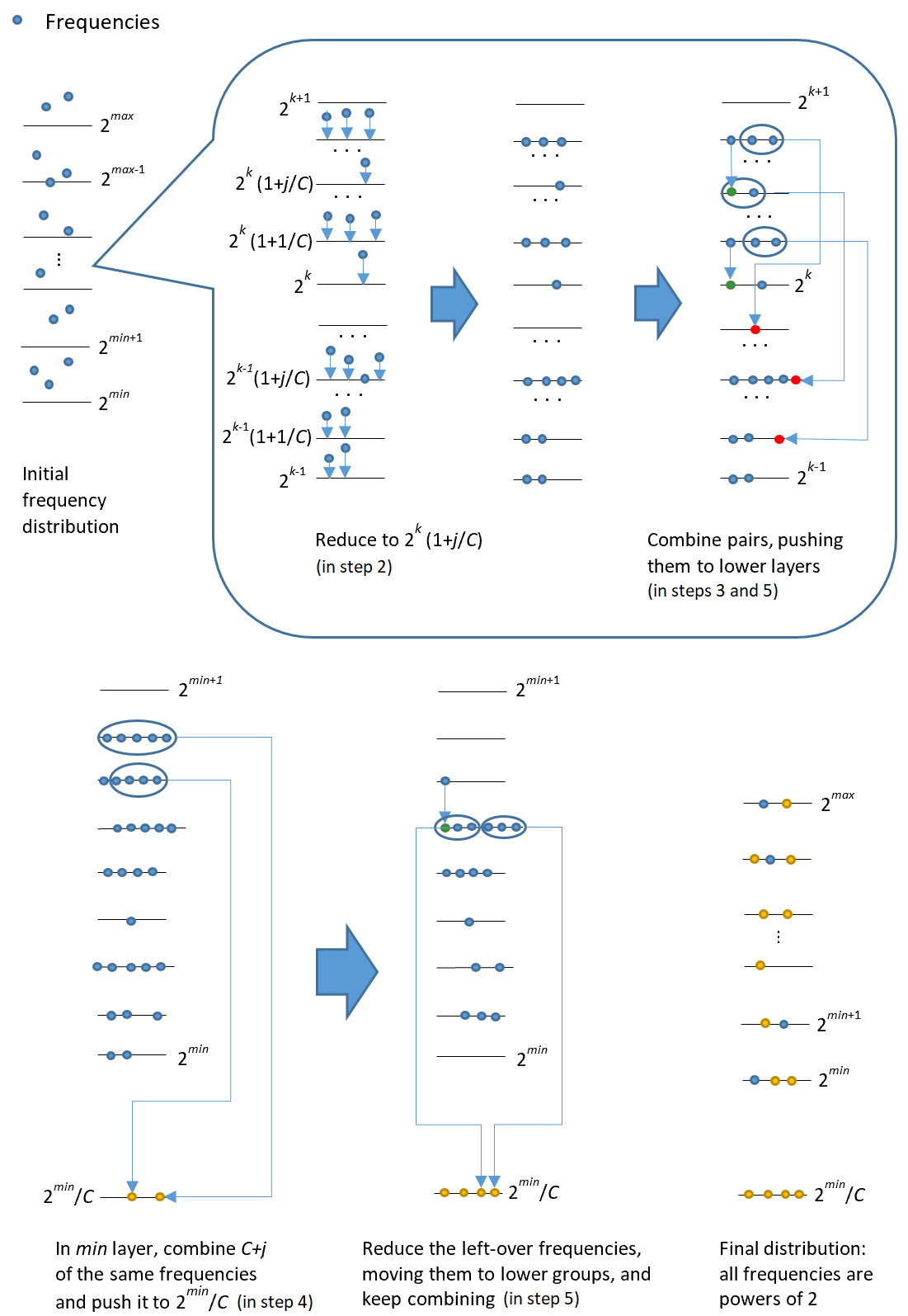
The Main Algorithm
Input: BGT instance $I=(h_{1}\geq h_{2}\geq\dots\geq h_{n})$.
Output: A (cyclic) perpetual schedule of $I$ specified by pairs $(p_{i},q_{i})$, for $1\leq i\leq n$. Item $b_{i}$ occurs in the schedule at positions $p_{i}+kq_{i}$, for $k\geq 0$.

1. Set the parameter $\delta=3\sqrt{h_{1}/H}\leq 3$.

   Form a pseudo-instance $\langle f^{\prime\prime}_{1}\leq f^{\prime\prime}_{2}\leq\ldots\leq f^{\prime\prime}_{n}\rangle$ of Pinwheel, by setting $f^{\prime\prime}_{i}=(1+\delta)H/h_{i}$. The density of this pseudo-instance is $\sum_{i}1/f_{i}^{\prime\prime}={1}/(1+\delta)$, and the setting of the parameter $\delta$ implies that $f^{\prime\prime}_{1}\geq 4$, regardless of the value of $h_{1}$. Let ${min}\geq 2$ be the largest integer such that $2^{min}\leq f^{\prime\prime}_{1}$ and let $max\geq min$ be the smallest integer such that $2^{max+1}>f^{\prime\prime}_{n}$.

2. Reduce each frequency $f^{\prime\prime}_{i}$ to the closest value $f_{i}$ of the form $2^{k}\left(1+\frac{j}{C}\right)$, where $k$, $C$ and $j$ are integers such that $k\geq min$, $C=2^{q}\geq 2$ for $q=\lfloor min/2\rfloor\geq 1$, and $0\leq j\leq C-1$. These conditions imply that the new frequencies $f_{i}$ are integral. Since the reduction of $f^{\prime\prime}_{i}$ to $f_{i}=2^{k}\left(1+\frac{j}{C}\right)$ is by a factor less than $1+\frac{1}{C}$, the density of the whole sequence of frequencies increases at most by a factor of $1+\frac{1}{C}$, to at most ${\left(1+\frac{1}{C}\right)}/{(1+\delta)}$.

   The sequence $\langle f_{1},f_{2},\ldots,f_{n}\rangle$ is our (proper) instance $V(I,\delta)$ of the Pinwheel problem. The remaining steps compute a schedule of this sequence. Steps 3-5 use Observations 1 and 2, and further reductions of the frequencies if needed, to transform the sequence $\langle f_{1},f_{2},\ldots,f_{n}\rangle$ to a sequence $\langle g_{1},g_{2},\ldots,g_{r}\rangle$, $r\leq n$ where all frequencies $g_{i}$ are powers of $2$.

3. We refer to the range $[2^{k},2^{k+1})$ of frequencies as layer $k$, and to the set of frequencies of the same value $2^{k}\left(1+\frac{j}{C}\right)$ as the group $j$ in layer $k$.

   For $k=max,max-1,\ldots,min+1$, apply Observation 1 in layer $[2^{k},2^{k+1})$ as many times as possible to combine pairs of the same frequencies $2^{k}\left(1+\frac{j}{C}\right)$, $1\leq j\leq C-1$, pushing them down to the lower layer by replacing each such pair with one frequency $2^{k-1}\left(1+\frac{j}{C}\right)$ (see the top half of Figure 1).

   On the conclusion of this step, there is at most one frequency $2^{k}\left(1+\frac{j}{C}\right)$, for each combination of $k\in[min+1,max]$ and $j\in[1,C-1].$

4. Apply Observation 2 in the layer $[2^{min},2^{min+1})$ until there are at most $C+j-1$ frequencies $2^{min}\left(1+\frac{j}{C}\right)$ left, for any $j\in[1,C-1]$ (see the first part of the bottom half of Figure 1).

5. For $k=max,max-1,\ldots,min$, reduce all remaining frequencies in range $[2^{k},2^{k+1})$ which are not powers of $2$, group by group starting from the top group defined by $j=C-1$, and pushing each frequency down to the next lower group. While progressing down through the groups, keep applying Observation 1 whenever possible, if in a layer $k\geq min+1$, and Observation 2 in the lowest layer for $k=min$.

   On the conclusion of this step, we have a sequence of frequencies $\langle g_{1},g_{2},\ldots,g_{r}\rangle$, $r\leq n$, which are powers of $2$, but the density further increases by some value $\Delta D\geq 0$. Thus the density of this final powers-of-$2$ instance $\langle g_{i}\rangle$ of the Pinwheel problem is at most ${\left(1+\frac{1}{C}\right)}/{(1+\delta)}+\Delta D$. We will show that the setting of the parameters $\delta$ and $C$ imply that this bound is at most $1$, so the Pinwheel sequence $\langle g_{i}\rangle$ is feasible.

6. Compute a cyclic schedule for the sequence of frequencies $\langle g_{1},g_{2},\ldots,g_{r}\rangle$ using the algorithm for powers-of-2 Pinwheel instances from [26]. Such a schedule is specified by pairs $(p_{i},q_{i})$, for $1\leq i\leq r$, which mean that the frequency $g_{i}$ is placed in the perpetual schedule of $\langle g_{1},g_{2},\ldots,g_{r}\rangle$ at positions $p_{i}+kq_{i}$, for $k\geq 0$.

   Expand the schedule of $\langle g_{1},g_{2},\ldots,g_{r}\rangle$ to a schedule of $\langle f_{1},f_{2},\ldots,f_{n}\rangle$ by tracing back the applications of Observations 1 and 2. The schedule of $\langle f_{1},f_{2},\ldots,f_{n}\rangle$ is returned as the computed schedule of the BGT input instance $(h_{1},h_{2},\ldots,h_{n})$.

Figure 2: Illustration of combining frequencies in the Main Algorithm. In steps 3–5 of the algorithm, frequency $f_{j}$ is paired twice with other frequencies by applications of Observation 1, creating a frequency $f_{j}/4$ (node $a$). The resulting frequency is then put into a group of $10$ frequencies $f_{j}/4$ and this group is replaced with one new frequency $g_{i}=f_{j}/40$ by an application of Observation 2.

The final step 6 of the algorithm is illustrated by an example given in Figure 2. In this example, a frequency $f_{j}$ (computed in step 2) was subsequently (in steps 3–5) paired twice with other frequencies by applications of Observation 1 (contributing first to a new frequency $f_{j}/2$ and then to a new frequency $f_{j}/4$) and ended up in a group of $10$ equal frequencies $f_{j}/4$. These $10$ frequencies were replaced with one new frequency $g_{i}=f_{j}/40$ by an application of Observation 2. Let the pair $(p_{i},q_{i})$ represent the positions of $g_{i}$ in the computed cyclic schedule of $\langle g_{1},g_{2},\ldots,g_{r}\rangle$: frequency $g_{i}$ is placed at positions $p_{i}+kq_{i}$, for $k\geq 0$.

Expanding the schedule of $\langle g_{1},g_{2},\ldots,g_{r}\rangle$ to the schedule of $\langle f_{1},f_{2},\ldots,f_{n}\rangle$, every $40$-th occurrence of frequency $g_{i}$ is replaced by frequency $f_{j}$. More precisely, we first replace every $10$-th occurrence of $g_{i}$ with the frequency $a=f_{j}/4$, starting from the $4$-th occurrence of $g_{i}$. Then every second occurrence of $a$ is replaced with $y=f_{j}/2$, starting from the $2$-nd occurrence of $a$, and finally every other occurrence of $y$ is replaced with $v=f_{j}$. Thus frequency $f_{j}$ is placed in the schedule at positions $(p_{i}+13q_{i})+k(40q_{i})$.

Theorem 4.1

For each BGT input instance, the Main Algorithm computes a $(1+3\sqrt{h_{1}/H})$-approximation schedule.

Proof

We show that the density of the sequence of frequencies $\langle g_{1},g_{2},\ldots,g_{r}\rangle$ computed in step 5 of the algorithm is at most $1$. Since these frequencies are powers of $2$, the sequence $\langle g_{1},g_{2},\ldots,g_{r}\rangle$ is feasible and gives a $(1+\delta)$-approximation schedule for the initial BGT input instance (Lemma 1).

The density of the Pinwheel pseudo-instance $\langle f^{\prime\prime}_{1},f^{\prime\prime}_{2},\ldots,f^{\prime\prime}_{n}\rangle$ is $D^{\prime\prime}=1/(1+\delta)$. To bound the density $D$ of the Pinwheel instance $\langle f_{1},f_{2},\ldots,f_{n}\rangle$, observe that if $f_{i}=2^{k}\left(1+{j}/{C}\right)$, then $f_{i}$ has been obtained from the rational frequency $f_{i}^{\prime\prime}$ such that

$$2^{k}\left(1+\frac{j}{C}\right)\leq f^{\prime\prime}_{i}<2^{k}\left(1+\frac{j+1}{C}\right).$$

This means that

$$f_{i}=2^{k}\left(1+\frac{j}{C}\right)>f^{\prime\prime}_{i}\left(1+\frac{j}{C}\right)/\left(1+\frac{j+1}{C}\right)=f^{\prime\prime}_{i}\frac{C+j}{C+j+1}\geq f^{\prime\prime}_{i}\frac{C}{C+1},$$

so

$$D<(1+1/C)D^{\prime\prime}=(1+1/C)/(1+\delta).$$

Steps 3 and 4 of the algorithm transform the Pinwheel instance $\langle f_{1},f_{2},\ldots,f_{n}\rangle$ using Observations 1 and 2, but without changing its density.

Step 5 further transforms the sequence of frequencies, increasing the density of the sequence whenever individual frequencies are reduced. We bound separately the increase $\Delta D_{above}$ of the density when we modify the frequencies in layers $max,max-1,\ldots,min+1$, and the increase $\Delta D_{min}$ of the density when we modify the frequencies in layer $min$.

$$\Delta D_{above} \leq \sum_{k=min+1}^{max}\sum_{j=1}^{C-1}\frac{1}{2^{k}}\left(\frac{1}{1+(j-1)/C}-\frac{1}{1+j/C}\right)$$

$$= \sum_{k=min+1}^{max}\frac{1}{2^{k}}\left(1-\frac{1}{1+(C-1)/C}\right)\leq\frac{1}{2^{min}}\cdot\frac{C-1}{2C-1}\,.$$

$$\Delta D_{min} \leq \sum_{j=1}^{C-1}(C+j-1)\frac{1}{2^{min}}\left(\frac{1}{1+(j-1)/C}-\frac{1}{1+j/C}\right)$$

$$= \frac{C}{2^{min}}\cdot\sum_{j=1}^{C-1}\frac{1}{C+j}\,.$$

Let $K=2^{min}/C^{2}\in\{1,2\}$. Then the density of the final powers-of-two Pinwheel instance $\langle g_{1},g_{2},\ldots,g_{r}\rangle$ is at most

$$\hskip-11.38109ptD+\Delta D_{above}+\Delta D_{min}$$ (1)

$$\leq \frac{1+1/C}{1+\delta}+\frac{1}{2^{min}}\cdot\frac{C-1}{2C-1}+\frac{C}{2^{min}}\cdot\sum_{j=1}^{C-1}\frac{1}{C+j}$$

$$= \frac{1+1/C}{1+\delta}+\frac{1}{KC}\cdot\left(\frac{C-1}{C\cdot(2C-1)}+\sum_{j=1}^{C-1}\frac{1}{C+j}\right)$$

$$= \frac{1+1/C}{1+\delta}+\frac{1}{KC}\cdot\left(\frac{1}{C}-\frac{1}{2C-1}+\sum_{j=1}^{C-1}\frac{1}{C+j}\right)$$

$$= \frac{1+1/C}{1+\delta}+\frac{1}{KC}\cdot\sum_{j=C}^{2C-2}\frac{1}{j}$$

$$\leq \frac{1+1/C}{1+\delta}+\frac{1}{KC}\cdot\ln 2$$ (2)

$$= \frac{1}{1+\delta}+\frac{1}{C}\cdot\left(\frac{1}{1+\delta}+\frac{\ln 2}{K}\right)$$

$$\leq \frac{1}{1+\delta}+\frac{\sqrt{2K}}{3}\cdot\frac{\delta}{\sqrt{1+\delta}}\cdot\left(\frac{1}{1+\delta}+\frac{\ln 2}{K}\right)$$ (3)

$$\leq 1.$$ (4)

To get Equality (1), use $2^{min}=KC^{2}$. To get Inequality (2), use the known fact that for the harmonic numbers $H_{k}=1+1/2+1/3+1/4+...+1/k$, we have $H_{k}=\ln k+\delta_{k}$, where $(\delta_{k})$ is a sequence of positive numbers strictly monotonically decreasing. Hence, we have $H_{2k}-H_{k}=\ln 2+\delta_{2k}-\delta_{k}<\ln 2$. To get Inequality (3), use

$$C\cdot\sqrt{2K}=\sqrt{2^{min+1}}>\sqrt{f^{\prime\prime}_{1}}=\sqrt{(1+\delta)\frac{H}{h_{1}}}=\frac{3\sqrt{1+\delta}}{\delta}\,.$$

Inequality (4) follows from the fact that for $0\leq\delta\leq 3$ and $K\in\{1,2\}$, the function $f_{K}(\delta)$ in line (3) is maximized for $\delta=0$. To see this, substitute $\gamma\equiv\sqrt{\delta+1}$ (so for $\delta$ increasing from $0$ to $3$, $\gamma$ increases from $1$ to $2$) to obtain

$$f_{K}(\delta)-1=f_{K}(\gamma^{2}-1)-1 = \frac{1}{\gamma^{2}}+\frac{\sqrt{2K}}{3}\cdot\frac{(\gamma^{2}-1)}{\gamma}\cdot\left(\frac{1}{\gamma^{2}}+\frac{\ln 2}{K}\right)-1$$ (5)

$$= \frac{\gamma^{2}-1}{3\gamma^{3}}\left(\frac{\sqrt{2}\ln 2}{\sqrt{K}}\gamma^{2}-3\gamma+{\sqrt{2K}}\right).$$

The quadratic in the parentheses in (5) has two distinct real roots

$$\frac{3\pm\sqrt{9-8\ln 2}}{2\sqrt{2}\ln 2/\sqrt{K}}.$$

For both $K\in\{1,2\}$, the smaller root $r_{K,1}$ is less than $1$ ($r_{1,1}<r_{2,1}=0.823...$) and the larger root $r_{K,2}$ is greater than $2$ ($r_{2,2}>r_{1,2}=2.478...$). This means that (5) is equal to $0$ for $\gamma=1$ and negative for $\gamma\in(1,2]$, or equivalently, $f_{K}(\delta)-1$ is equal to $0$ for $\delta=0$ and negative for $\delta\in(0,3]$. $\Box$

The discussion in Section 3 and Theorem 4.1 imply the following corollary.

Corollary 1

For Pinwheel instances $2\leq f_{1}\leq f_{2}\leq\ldots\leq f_{n}$, the Main Algorithm applied to sequences $(1/f_{1},1/f_{2},\ldots,1/f_{n})$ is a Pinwheel scheduler with the guarantee density threshold $1-3/\sqrt{f_{1}}$. Thus each Pinwheel instance with density at most $1-3/\sqrt{f_{1}}$ is feasible.

Theorem 4.2

The Main Algorithm can be implemented so that its running time is $O(n\log n)$, assuming constant-time operations on real numbers, including the logarithm operation and rounding.

Proof

Steps 1 and 2 take linear time (or $O(n\log n)$, if the input sequence is not provided in the sorted order). In steps 3–5, the non-empty groups are maintained in a dictionary data structure, which can be created in $O(n\log n)$ time.

In steps 3 and 4, the groups are considered in the decreasing order (from the highest group in the highest layer). In step 3, if two frequencies are paired by Observation 1, then the group to which the new frequency should be added can be found (or created, if empty) in $O(\log n)$ time. This can happen only $O(n)$ times, since each pairing reduces the number of frequencies, so step 3 takes $O(n\log n)$ time. In step 4, if $m$ frequencies are combined by Observation 2 into one new frequency $2^{min}/C$, then the required computation takes $O(m)$ time (in this case, no need to look for the group with frequencies $2^{min}/C$). Thus step 4 takes $O(n)$ time.

In step 5, the groups are again considered in the decreasing order. For each group, frequencies are paired by Observation 1 or combined by Observation 2 (as above, all this computation takes $O(n\log n)$ time) and the remaining frequencies are appended to the next non-empty group in constant time. Thus step 5 takes $O(n\log n)$ time.

Step 6, the computation of a cyclic schedule of the feasible powers-of-2 frequencies $\langle g_{1},g_{2},\ldots,g_{r}\rangle$, is done by the following algorithm from [26], which can be implemented to run in linear time, assuming that the input sequence is sorted. Take two largest frequency values $g_{r-1}$ and $g_{r}$, replace them with a new frequency $g^{\prime}=2g_{r-1}$ and compute a cyclic schedule for the new $(r-1)$-element sequence. To get a schedule for the original sequence $\langle g_{1},g_{2},\ldots,g_{r}\rangle$, replace the occurrences of $g^{\prime}$ with alternating occurrences of $g_{r-1}$ and $g_{r}$. That is, if $g^{\prime}$ occurs at positions $p+kq$, for $k\geq 0$, then $g_{r-1}$ occurs at positions $p+2kq$ and $g_{r}$ occurs at positions $p+(2k+1)q$, for $k\geq 0$.

During the computation in steps 3–5, the pairing and combining of frequencies is recorded in ordered trees as illustrated in Figure 2. The additional time required to create one such tree is linear in the size of the tree, so $O(n)$ time for creating all trees. By traversing these trees, we can expand in $O(n)$ time the cyclic schedule of $\langle g_{1},g_{2},\ldots,g_{r}\rangle$ to a cyclic schedule of $\langle f_{1},f_{2},\ldots,f_{n}\rangle$.

The Main Algorithm computes the representation of a cyclic schedule in the form of pairs $(p_{i},q_{i})$, which enables constant-time answers to queries: given the current step $T$, when will be the next step when a given element $b_{i}$ is serviced? To generate the schedule step by step, taking $O(\log n)$ time per step, maintain a priority queue (e.g. as the heap data structure) with the pairs $(i,t_{i})$, where $i=1,2,\ldots,n$ and $t_{i}$ is the next step when element $b_{i}$ will be serviced. Initially the priority queue contains pairs $(i,p_{i})$. For the current step of the schedule, remove from the priority queue the pair $(i,t_{i})$ with the smallest $t_{i}$, schedule the element $b_{i}$, and insert to the priority queue the pair $(i,t_{i}+q_{i})$. $\Box$

5 Improved approximation for the general case

In this section, we consider general approximation (upper) bounds of polynomial BGT algorithms, that is, bounds on the approximation ratios which hold for any BGT input, irrespectively of its characteristics. Comparing with the best previous general bound of $12/7$ given in [40], we show a BGT algorithm with approximation ratio not greater than $8/5+o(1)<12/7$. We assume throughout this section that the growth rates are normalized to $H=1$.

Our algorithm uses the approximation algorithm from Section 4.2, which computes $(1+o(1))$-approximation schedules, if the highest growth rate $h_{1}$ is $o(1)$. The algorithm first partitions the input set $I$ into two groups $S$ and $L$, separating bamboos with small growth rates of values $o(1)$ from bamboos with large growth rates. Then schedules ${\cal S}$ for $S$ and ${\cal L}$ for $L$ are computed separately, and finally these two schedules are merged into the final schedule ${\cal I}$ for the whole input $I$. The schedule ${\cal S}$ for the small rates is computed using the approximation algorithm from Section 4.2, so ${\mbox{\it MH}}({\cal S})\leq H(S)+o(1)$. The schedule ${\cal L}$ for the large rates is either an optimal schedule, computed using exhaustive search, or an approximation schedule computed by the 2-approximation algorithm which we mentioned in Section 4.1. The choice depends on the parameters of $L$ and $S$. In the former case, we use the bound ${\mbox{\it MH}}({\cal L})={\mbox{\it OPT}}(L)\leq{\mbox{\it OPT}}(I)$ in the analysis of the approximation ratio, while in the latter case, we use the bound ${\mbox{\it MH}}({\cal L})\leq 2\cdot H(L)$.

We summarise this result in the theorem stated below and the remaining part of this section is the proof of this theorem. In our case analysis, for some cases we need to separate the fastest growing bamboo $b_{1}$ from the set $L$, getting a partition of $I$ into three sets $B=\{b_{1}\}$, $L$ and $S$, and computing schedules ${\cal S}$ and ${\cal L}$ for $S$ and $L$ as above. The final schedule ${\cal I}$ for the whole input $I$ is defined by a pattern in which the schedules ${\cal S}$ and ${\cal L}$, and cutting $b_{1}$ (if $b_{1}$ is separated from $L$) are interleaved. For example, if ${\cal I}$ is defined by the pattern $(L,B,L,S)$, then the schedule ${\cal L}$ is put in ${\cal I}$ in every other position starting from position $1$, the schedule ${\cal S}$ is in every fourth position starting from position $4$, and $b_{1}$ occupies the remaining positions.

Theorem 5.1

There is a polynomial-time algorithm which for any instance $I$ of the BGT problem, computes a $(8/5+o(1))$-approximation schedule.

The basic split of the input sequence.

We partition $I$ into two groups of large growth rates $L=\{b_{i}:h_{i}\geq 1/m\}$ and small growth rates $S=\{b_{i}:h_{i}<1/m\}$. We set the threshold value $m=\log n/(4\log\log n)$, where $\log x$ stands here for $\log_{2}(x)$, if $x>1$, or for $1$, if $x\leq 1$ (so $m$ is well-defined and positive for all integers $n\geq 2$). Observe that $m<n$, so $S$ is never empty, but $L$ can be empty, if there are no large growth rates. We define $\bar{L}=H(L)=\sum_{b_{i}\in L}h_{i}$ and $\bar{S}=H(S)$, so $\bar{L}+\bar{S}=1$. Generally, if $A$ is a subset of bamboos, then $\bar{A}$ denotes the sum of the rates of bamboos in $A$. Let ${\cal S}$ be a schedule for $S$ computed by the approximation algorithm from Section 4.2. If $\bar{S}=\Omega(1)$, then ${\mbox{\it MH}}({\cal S})=\bar{S}(1+o(1))$, and if $\bar{S}=o(1),$ then ${\mbox{\it MH}}({\cal S})\leq 2\bar{S}=o(1)$, so in both cases ${\mbox{\it MH}}({\cal S})=\bar{S}+o(1)$.

Fact 1

An optimal schedule for the growth rates $L$ can be computed in $o(n)$ time.

Proof

The lower bound of $1/m$ on the growth rates in $L$ imply that $|L|\leq m$. Since ${\mbox{\it OPT}}(L)\leq 2\bar{L}\leq 2$, then in an optimal schedule for $L$, every bamboo can have at most $2m$ different heights. This means that the number of configurations to consider is at most $(2m)^{m}$, where a configuration is an $|L|$-tuple of possible heights of the bamboos in $L$, as observed just before the next cutting. Each (infinite) schedule $\ell=(i_{1},i_{2},\ldots)$ can be represented as a sequence of configurations $(C_{1},C_{2},\ldots)$. If this sequence is $(C_{1},C_{2},\ldots,C_{k},C_{k+1},\ldots,C_{k+p},\ldots)$, where $C_{k+1}=C_{k+p}$ is the first repeat of the same configuration, then for the periodic schedule $\ell^{*}$ formed as $(i_{1},i_{2},\ldots,i_{k})$ followed by repetitions of $(i_{k+1},\ldots,i_{k+p})$, we have ${\mbox{\it MH}}(\ell)^{*}\leq{\mbox{\it MH}}(\ell)$. Hence, there is an optimal schedule which is periodic, where $k$ (the length of the initial sequence of distinct configurations) and $p$ (the length of the period) are both at most $(2m)^{m}$. Such a periodic optimal schedule can be found by an exhaustive search, or any better search strategy which guarantees taking into account all periodic schedules.

This type of argument – a configuration space of finite size and finitely many feasible structures – has been used previously in analyses of processes of similar nature. For example, in the context of computing a perpetual schedule of maintaining machines, such an argument was used by Anily et al. [2].

We provide further details to justify our choice of $m$. We have set the value of $m$ appropriately small in terms of $n$, so that the following algorithm finds an optimal schedule for $L$ in $o(n)$ time. Let $G$ be the directed graph of the configurations space: the vertices are the configurations with height at most $2|L|$ (that is, with the maximum height of bamboo at most $2|L|$), and each edge is a possible one-round change from the current configuration to another one, defined by cutting a given bamboo. This graph has at most $(2m)^{m}$ vertices and each vertex has at most $|L|\leq m$ outgoing edges (at each configuration, there are $|L|$ choices of a bamboo for cutting, but some choices may take the maximum height of a bamboo above the $2|L|$ threshold). For any positive number $M$, ${\mbox{\it OPT}}(L)\leq M$, if and only if, the subgraph of $G$ induced by all configurations with height at most $M$ has a cycle reachable from the initial configuration $(h_{j}:j\in L)$ (the configuration just before the first cutting). Thus we can find ${\mbox{\it OPT}}(L)$, and an optimal schedule for $L$, by binary search over the $O(m^{2})$ possible heights of configurations (each bamboo has at most $2m$ possible heights). In this binary search, one iteration takes time linear in the size of graph $G$, so the total running time is $O((2m)^{m}m\log m)=O(n^{1/2})$. $\Box$

Fact 2

For the set $S$, if $\bar{S}=\Omega(1),$ then the algorithm of Section 4.2 computes a $(1+o(1))$-approximation schedule $\cal S$ for $S$ in $O(n\log n)$ time.

Proof

A direct consequence of Theorems 4.1 and 4.2. $\Box$

If $L=\emptyset$, then we have a $(1+o(1))$-approximation for the whole instance $I$ from Fact 2, so from now on we assume that $L\not=\emptyset$. We consider separately the cases specified below. The $(8/5+o(1))$-approximation factor follows because for each case and each $b\in I$, we either establish that the maximum height of $b$ in ${\cal I}$ is at most $8/5+o(1)$, or we establish that it is at most ${\mbox{\it OPT}}(I)(8/5+o(1))$.

Case 1:

$|L|\geq 2,\;$ $0<\bar{S}\leq 2/5,$

Case 2:

$|L|\geq 2,\;$ $2/5<\bar{S}\leq 8/15,\;$ $h_{1}\leq 8/25$,

Case 3:

$|L|\geq 2,\;$ $2/5<\bar{S}\leq 8/15,\;$ $h_{1}>8/25$,

Case 4:

$|L|\geq 2,\;$ $8/15<\bar{S}\leq 3/5,$

Case 5:

$|L|\geq 1,\;$ $3/5<\bar{S}<1$,

Case 6:

$|L|=1,\;$ $0<\bar{S}\leq 3/5$.

Case 1: $|L|\geq 2,$ $0<\bar{S}\leq 2/5$. We use an optimal schedule ${\cal L}$ for $L$ and the pattern $(L,L,L,S)$. We obtain a schedule ${\cal I}$ where the bamboos in $S$ stay within the height $4\cdot(\bar{S}+o(1))\leq 8/5+o(1)$. For any $b\in L$, if $f$ denotes the frequency of $b$ in ${\cal L}$, that is, the longest time, in rounds, between two consecutive cuts of $b$ in ${\cal L}$, then the frequency of $b$ in ${\cal I}$ is at most $f+\lceil f/3\rceil$ (for two consecutive cuts of $b$ in $\cal L$, we are adding between them in ${\cal I}$ at most $\lceil f/3\rceil$ cuts from sequence ${\cal S}$). Thus the height of $b$ in ${\cal I}$ is never greater than

$$(f+\lceil f/3\rceil)h_{b} = fh_{b}\left(1+\frac{\lceil f/3\rceil}{f}\right)\leq{\mbox{\it OPT}}(L)\left(1+\frac{\lceil f/3\rceil}{f}\right)$$ (6)

$$\leq {\mbox{\it OPT}}(I)\left(1+\frac{\lceil f/3\rceil}{f}\right)\leq\frac{3}{2}{\mbox{\it OPT}}(I).$$

The last inequality holds because for $f\geq 2$, $\lceil f/3\rceil\leq f/2$.

Case 2: $|L|\geq 2,$ $2/5<\bar{S}\leq 8/15,$ $h_{1}\leq 8/25$. We use an optimal schedule ${\cal L}$ for $L$ and the pattern $(L,L,S)$. For any $b\in S$, its height in ${\cal I}$ is at most $3\cdot(\bar{S}+o(1))\leq 8/5+o(1)$. For any $b\in L$, its frequency $f$ in ${\cal L}$ increases to at most $f+\lceil f/2\rceil$ in ${\cal I}$, since now for two consecutive cuts of $b$ in $\cal L$, we are adding in ${\cal I}$ at most $\lceil f/2\rceil$ cuts from sequence ${\cal S}$. Thus, following a similar argument as in (6), the height of $b$ in ${\cal I}$ is at most ${\mbox{\it OPT}}(I)(1+\lceil f/2\rceil/f)$. The factor $1+\lceil f/2\rceil/f$ is at most $8/5$ for each $f\geq 2$ except $f=3$ (we have $\lceil f/2\rceil\leq(3/5)f$ for each integer $f\geq 2$ except $f=3$). If $f=3$, then the height of $b$ in ${\cal I}$ is at most $(f+\lceil f/2\rceil)h_{1}=5h_{1}\leq 8/5$.

Case 3: $|L|\geq 2,$ $2/5<\bar{S}\leq 8/15,$ $h_{1}>8/25$. We remove $b_{1}$ from $L$ and put it in a separate singleton set $B$, and we move some bamboos from $S$ to $L$, to obtain a partition of $I$ into three sets $B=\{b_{1}\}$, $S^{\prime}$ and $L^{\prime}$ such that $\bar{S^{\prime}}=2/5+o(1)$ and $\bar{L^{\prime}}\leq 3/5-h_{1}$. This is feasible, because all growth rates in $S$ are $o(1)$. The set $L^{\prime}$ may now be large, with size up to linear in $n$, but from this case on, we do not compute an optimal schedule for $L^{\prime}$, using instead a schedule ${\cal L^{\prime}}$ computed by the 2-approximation algorithm mentioned in Section 4.1, which runs in $O(n\log n)$ time. For set $S^{\prime}$, we use a schedule ${\cal S^{\prime}}$ computed by the approximation algorithm from Section 4.2.

The final schedule ${\cal I}$ is defined by the pattern $(L^{\prime},B,L^{\prime},S^{\prime})$, if $8/25<h_{1}\leq 2/5$, or the pattern $(B,L^{\prime},B,S^{\prime})$, if $h_{1}>2/5$. In both cases, the height of any $b\in S^{\prime}$ in ${\cal I}$ is at most $4(2/5+o(1))=8/5+o(1)$. In the former case, for any $b\in L^{\prime}$, the height of $b$ in ${\cal L^{\prime}}$ is at most $2\bar{L^{\prime}}$, so at most $4\bar{L^{\prime}}\leq 4(3/5-h_{1})\leq 28/25<8/5$ in ${\cal I}$, and the height of $b_{1}$ is at most $4h_{1}\leq 8/5$. In the latter case, for any $b\in L^{\prime}$, the height of $b$ in ${\cal L^{\prime}}$ is at most $2\bar{L^{\prime}}$, so at most $8\bar{L^{\prime}}\leq 8(3/5-h_{1})\leq 8/5$ in ${\cal I}$, and the height of $b_{1}$ is at most $2h_{1}\leq{\mbox{\it OPT}}(I)$.

Case 4: $|L|\geq 2,$ $8/15<\bar{S}\leq 3/5$. We move some bamboos from $S$ to $L$, to obtain a partition of $I$ into two sets $S^{\prime}$ and $L^{\prime}$ such that $\bar{S^{\prime}}=8/15+o(1)$, and $\bar{L^{\prime}}\leq 7/15$, and we compute schedules ${\cal S^{\prime}}$ and ${\cal L^{\prime}}$ as in the previous case. The final schedule ${\cal I}$ is defined by the pattern $(L^{\prime},L^{\prime},S^{\prime})$. The height of any $b\in S^{\prime}$ in ${\cal I}$ is at most $3(8/15+o(1))=8/5+o(1)$. As in Case 2, the frequency of any $b\in L^{\prime}$ increases from $f$ in ${\cal L}$ to at most $f+\lceil f/2\rceil$ in ${\cal I}$, so the maximum height of $b$ increases from $fh_{b}\leq 2\bar{L^{\prime}}\leq 14/15$ in ${\cal L}$ to at most $(f+\lceil f/2\rceil)h_{b}\leq(14/15)(1+\lceil f/2\rceil/f)\leq 8/5$ in ${\cal I}$. For the last inequality, recall from Case 2 that $\lceil f/2\rceil\leq(3/5)f$ for all $f\geq 2$ except $f=3$, and verify the $f=3$ case separately.

Case 5: $|L|\geq 1,$ $3/5<\bar{S}<1$. Move some bamboos from $S$ to $L$, to obtain a partition of $I$ into two sets $S^{\prime}$ and $L^{\prime}$ such that $\bar{S^{\prime}}=3/5+o(1)$ and $\bar{L^{\prime}}\leq 2/5$, compute schedules ${\cal S^{\prime}}$ and ${\cal L^{\prime}}$ as in the previous two cases, and define the final schedule ${\cal I}$ by the pattern $(L^{\prime},S^{\prime})$. The height of any $b\in S^{\prime}$ in ${\cal I}$ is at most $2(3/5+o(1))<8/5$, and the height of any $b\in L^{\prime}$ in ${\cal I}$ is at most $4\bar{L^{\prime}}\leq 8/5$.

Case 6: $|L|=1,$ $0<\bar{S}<3/5$. The set $I$ is partitioned into $B=\{b_{1}\}$ and $S=I-B$, and the final schedule ${\cal I}$ is defined by $(B,S)$. The height of $b\in S$ in ${\cal I}$ is at most $2(3/5+o(1))<8/5$, and the height of $b_{1}$ is at most $2h_{1}\leq OPT(I)$.

The running time of this approximation algorithm is dominated by the $O(n\log n)$ time of the approximation algorithm from Section 4.2.

6 Continuous BGT

We consider now the continuous variant of the BGT problem. Since this variant models scenarios when bamboos are spread over some geographical area, we will now refer not only to bamboos $b_{1},b_{2},\ldots,b_{n}$ but also to the points $v_{1},v_{2},\ldots,v_{n}$ (in the implicit underlying space) where these bamboos are located. We will denote by $V$ the set of these points.

Recall that input $I$ for the continuous BGT problem consists of the growth rates $(h_{i}:\>1\leq i\leq n)$ and the travel times between bamboos $(t_{i,j}:\>1\leq i,j\leq n)$. We assume that $h_{1}\geq h_{2}\geq\ldots\geq h_{n}$, as before, and normalize these rates, for convenience, so that $h_{1}+h_{2}+\ldots+h_{n}=H=1$ (this normalization is done without loss of generality, since only the relative heights of bamboos are relevant). We assume that the travel distances form a metric on $V$.

For any $V^{\prime}\subseteq V$, the minimum growth rate among all points in $V^{\prime}$ is denoted by $h_{\min}(V^{\prime})$, and the maximum growth rate among all points in $V^{\prime}$ is denoted by $h_{\max}(V^{\prime})$. Let $h_{\min}=h_{\min}(V)=h_{n}$, and $h_{\max}=h_{\max}(V)=h_{1}$. Recall that we assume $n\geq 2$ (to avoid the trivial case), and now we additionally assume that $h_{\max}>h_{\min}$ (the uniform case, when $h_{\max}=h_{\min}$, is TSP).

The diameter of the set $V$ is denoted by $D=D(V)=\max\{t_{i,j}:\>1\leq i,j\leq n\}$. For any $V^{\prime}\subseteq V$, ${\mbox{\it MST}}(V^{\prime})$ denotes the minimum weight of a spanning tree on $V^{\prime}$ (the travel times are the weights of the edges). Recall that for an algorithm ${\cal{A}}$ and input $I$, ${\mbox{\it MH}}({\cal{A}}(I))$ denotes the maximum height that any bamboo ever reaches, if trimming is done according to the schedule computed by ${\cal{A}}$, and ${\mbox{\it OPT}}(I)$ is the optimal (minimal) maximum height of a bamboo over all schedules.

6.1 Lower bounds and simple approximation based on discrete BGT

We first show some simple lower bounds on the maximum height of a bamboo. For notational brevity, we omit the explicit reference to the input $I$. For example, the inequality ${\mbox{\it MH}}({\cal{A}})\geq Dh_{\max}$ in the lemma below is to be understood as ${\mbox{\it MH}}({\cal{A}}(I))\geq D(V(I))\cdot h_{\max}(V(I))$, for each input instance $I$.

Lemma 3

${\mbox{\it MH}}({\cal{A}})\geq Dh_{\max}$, for any algorithm ${\cal{A}}$.

Proof

The robot must visit another point $x$ in $V$ at distance at least $D/2$ from $v_{1}$. When the robot comes back to $v_{1}$ after visiting $x$ (possibly via a number of other points in $V$), the bamboo at $v_{1}$ has grown at least to the height of $Dh_{1}=Dh_{\max}$. $\Box$

Lemma 4

${\mbox{\it MH}}({\cal{A}})\geq h_{\min}(V^{\prime})\cdot{\mbox{\it MST}}(V^{\prime}),$ for any algorithm ${\cal{A}}$ and $V^{\prime}\subseteq V$.

Proof

Let $v$ be the point in $V^{\prime}$ visited last: all points in $V^{\prime}\setminus\{v\}$ have been visited at least once before the first visit to $v$. The distance traveled until the first visit to $v$ is at least ${\mbox{\it MST}}(V^{\prime})$, so the bamboo at $v$ has grown to the height at least $h_{v}\cdot{\mbox{\it MST}}(V^{\prime})\geq h_{\min}(V^{\prime})\cdot{\mbox{\it MST}}(V^{\prime})$. $\Box$

One may ask how good are the schedules for continuous BGT which are computed taking into account only the growth rates, ignoring the travel times. If we use, for example, the schedules computed by the 2-approximation algorithm from Section 4, which guarantee that the maximum height of a bamboo does not grow above $2$ (recall that we normalize the growth rates, so $H=1$), then there are at most $\lfloor 2/h_{i}\rfloor-1$ cutting actions between two consecutive cuttings of bamboo $b_{i}$. Otherwise bamboo $b_{i}$ would grow in discrete BGT to the height at least $h_{i}(\lfloor 2/h_{i}\rfloor+1)>2=2H$. Thus in continuous BGT the time between two consecutive cuttings of bamboo $b_{i}$ is at most $D\lfloor 2/h_{i}\rfloor$, so the height of this bamboo is never greater than $h_{i}D\lfloor 2/h_{i}\rfloor\leq 2D$. Combining this with Lemma 3, we conclude that the 2-approximation algorithm for discrete BGT is a $(2/h_{\max})$-approximation algorithm for continuous BGT. In particular, this approach gives $\Theta(1)$-approximate algorithm for continuous BGT for inputs with $h_{1}=\Theta(1)$. To derive good approximation algorithms for other types of input, we will use the lower bound from Lemma 4.

6.2 Approximation algorithms

We present in this section three approximation algorithms for continuous BGT which are based on computing spanning trees. Algorithm 1 computes only one spanning tree of all points and the schedule for the robot is to traverse repeatedly an Euler tour of this tree. This simple algorithm ignores the growth rates of bamboos and computes a schedule of cutting taking into account only the travel times between points.

Algorithms 2 and 3 group the bamboos according to the similarity of their growth rates and compute a separate spanning tree for each group. The robot moves from one tree to the next in the Round-Robin fashion. At each spanning tree $T$, the robot walks along the Euler-tour of this tree for time $D$ before moving to the next tree. When the robot eventually comes back to tree $T$, it resumes traversing the Euler tour of $T$ from the point when it last left this tree. The growth rates of bamboos in the same spanning tree are within a factor of 2. Algorithm 3 differs from Algorithm 2 by using spanning trees only for the first $\Theta(\log n)$ groups, which include bamboos with growth rates greater than $1/n^{2}$. The remaining bamboos, which all have low growth rates, are dealt with individually.

We describe our Algorithms 1, 2 and 3 in pseudocode and give their approximation ratio in the theorems below. The description of each algorithm consists of two parts: pre-processing and walking. We do not explicitly mention the actions of cutting/attending bamboos, assuming that whenever the robot passes a point in $V$​, it cuts the bamboo growing at this point.

 

Algorithm 1: An $O({h_{\max}}/{h_{\min}})$-approximation algorithm for continuous BGT.

1. [Pre-processing] Calculate a minimum spanning tree $T$ of the point set $V$.

2. [Walking] Repeatedly perform an Euler-tour traversal of $T$.

 

Theorem 6.1

Algorithm 1 is an $O({h_{\max}}/{h_{\min}})$-approximation algorithm for the continuous BGT problem.

Proof

Let ${\cal{A}}_{1}$ denote Algorithm 1. Every point $v_{i}\in V$ is visited by ${\cal{A}}_{1}$ at least every $2\cdot{\mbox{\it MST}}(V)$ time units. Hence,

$${\mbox{\it MH}}({\cal{A}}_{1})=O(h_{\max}(V)\cdot{\mbox{\it MST}}(V)).$$ (7)

According to Lemma 4,

$${\mbox{\it OPT}}=\Omega(h_{\min}(V)\cdot{\mbox{\it MST}}(V)).$$ (8)

Combining the two bounds (7) and (8), it follows that Algorithm 1 is an $O({h_{\max}}/{h_{\min}})$-approximation algorithm for BGT. $\Box$

 

Algorithm 2: An $O(\log\lceil{h_{\max}}/{h_{\min}}\rceil)$-approximation algorithm for continuous BGT.

1. [Pre-processing]

2. Let $s=\lfloor\log_{2}({h_{\max}}/{h_{\min}})\rfloor+1$.

3. For $i\in\{1,2\ldots,s\}$, let $V_{i}=\{v_{j}\in V\mid 2^{i-1}\cdot h_{\min}\leq h_{j}<2^{i}\cdot h_{\min}\}$.

4. for $i=1$ to $s$ such that $V_{i}\neq\emptyset$ do

5. Let $T_{i}$ be a minimum spanning tree on $V_{i}$.

6. Let $C_{i}$ be a directed Euler-tour traversal of $T_{i}$.

7. Set an arbitrary point on $C_{i}$ as the last visited point on $C_{i}$.

8. [Walking]

9. repeat forever

10. for $i=1$ to $s$ such that $V_{i}\neq\emptyset$ do

11. Walk to the last visited point on $C_{i}$.

12. If $V_{i}$ has at least $2$ points, then walk along $C_{i}$ in the direction of the tour,
         stopping as soon when the distance covered is at least $D$.

 

Theorem 6.2

Algorithm 2 is an $O(\log{\lceil h_{\max}}/{h_{\min}\rceil})$-approximation algorithm for the continuous BGT problem.

Proof

For any $i\in\{1,2,\ldots,s\}$, consider any point $v\in V_{i}$. The robot walks along one tree for at most distance $2D$ and then covers at most distance $D$ to move to the next tree. After a visit to point $v$, the robot comes back to tree $T_{i}$ at most $\left\lceil{2\cdot{\mbox{\it MST}}(V_{i})}/{D}\right\rceil$ times before visiting $v$ again. Therefore, recalling from the algorithm that there are at most $s=\lfloor\log_{2}({h_{\max}}/{h_{\min}})\rfloor+1$ trees, the distance traveled between two consecutive visits to point $v$ is at most

$$3Ds\left\lceil\frac{2\cdot{\mbox{\it MST}}(V_{i})}{D}\right\rceil \leq 3s(D+2\cdot{\mbox{\it MST}}(V_{i})).$$

Hence, the height of the bamboo at $v$ is always

$$O\left(h_{\max}(V_{i})\cdot\log\left\lceil\frac{h_{\max}}{h_{\min}}\right\rceil\cdot\max\{D,{\mbox{\it MST}}(V_{i})\}\right).$$ (9)

On the other hand, using Lemmas 3 and 4, we obtain

$${\mbox{\it OPT}}\;\geq\;h_{\min}(V_{i})\cdot\max\{D,{\mbox{\it MST}}(V_{i})\}.$$ (10)

Combining the two bounds (9) and (10), and observing that $h_{\max}(V_{i})\leq 2\cdot h_{\min}(V_{i})$, we obtain that the height of the bamboo at $v$ is always $O({\mbox{\it OPT}}\cdot\log\lceil{h_{\max}}/{h_{\min}}\rceil)$, so Algorithm 2 is an $O(\log\lceil{h_{\max}}/{h_{\min}}\rceil)$-approximation algorithm for BGT. $\Box$

 

Algorithm 3: An $O(\log n)$-approximation algorithm for continuous BGT.

1. [Pre-processing]

2. Let $s=\lceil 2\cdot\log_{2}n\rceil$.

3. Let $V_{0}=\{v_{i}\in V\mid h_{i}\leq n^{-2}\}$.  Let $V_{0}=\{v^{\prime}_{0},v^{\prime}_{1},\ldots,v^{\prime}_{\ell-1}\}.$

4. For $i\in\{1,2,\ldots,s\}$, let $V_{i}=\{v_{j}\in V\mid 2^{i-1}\cdot n^{-2}<h_{j}\leq 2^{i}\cdot n^{-2}\}$.

5. for $i=1$ to $s$ such that $V_{i}\neq\emptyset$ do

6. Let $T_{i}$ be a minimum spanning tree on $V_{i}$.

7. Let $C_{i}$ be a directed Euler-tour traversal of $T_{i}$.

8. Set an arbitrary point on $C_{i}$ as the last visited point on $C_{i}$.

9. [Walking]

10. $j=0$.

11. repeat forever

12. for $i=1$ to $s$ such that $V_{i}\neq\emptyset$ do

13. Walk to the last visited point on $C_{i}$.

14. If $V_{i}$ has at least $2$ points, then walk along $C_{i}$ in the direction of the tour,
         stopping as soon when the distance covered is at least $D$.

15. If $V_{0}\neq\emptyset$, then walk to $v^{\prime}_{j}$ and let $j=j+1\pmod{\ell}$.

 

Theorem 6.3

Algorithm 3 is an $O(\log n)$-approximation algorithm for the continuous BGT problem.

Proof

Each round of Algorithm 3, that is, each iteration of the repeat loop, is a cycle over all $s=\Theta(\log n)$ trees and a visit to one point in the set $V_{0}$. Consider any point $v\in V_{i}$, for any $i\in\{1,2,\ldots,s\}$. The distance traveled between two consecutive visits of $v$ is at most

$$(3Ds+D)\left\lceil\frac{2\cdot{\mbox{\it MST}}(V_{i})}{D}\right\rceil \leq (3s+1)(D+2\cdot{\mbox{\it MST}}(V_{i}))$$

$$= O(\log n\cdot\max\{D,{\mbox{\it MST}}(V_{i})\}).$$

Hence, the height of the bamboo at $v$ is always

$$O(h_{\max}(V_{i})\cdot\log n\cdot\max\{D,{\mbox{\it MST}}(V_{i})\}).$$

Using the lower bound (10) on OPT and the fact that $h_{\max}(V_{i})\leq 2\cdot h_{\min}(V_{i})$, we conclude that the height of the bamboo at $v$ is always $O({\mbox{\it OPT}}\cdot\log n)$.

Consider now a point $v\in V_{0}$. The distance traveled between two consecutive visits of $v$ is at most

$$(3Ds+D)|V_{0}|\;=\;O(n\cdot D\cdot\log n).$$

Hence, the height of the bamboo at $v$ is always

$$O(h_{\max}(V_{0})\cdot n\cdot D\cdot\log n)=O(n^{-2}\cdot n\cdot D\cdot\log n)=O(h_{\max}\cdot D\cdot\log n).$$

This and Lemma 3 imply that the height of the bamboo at $v$ is always $O({\mbox{\it OPT}}\cdot\log n)$. Thus Algorithm 3 is an $O(\log n)$-approximation algorithm for BGT. $\Box$

Note that the pre-processing in all Algorithms 1, 2 and 3 is dominated by the minimum-spanning tree computation, which can be implemented in $O(n^{2})$ time (e.g. by using Prim’s algorithm [36]). Then the running time to produce the schedule (the consecutive steps of the schedule) is constant per one step of the schedule.

6.3 How tight are the upper and lower bounds?

Our $O(\log n)$-approximation algorithm for the continuous BGT (Algorithm 3) can return schedules which are worse than the optimal schedules by a factor of $\Theta(\log n)$. For example, consider the input which consists of two sets $V^{\prime}$ and $V^{\prime\prime}$ of $n/2$ points each such that in each set the points are very close to each other (with the total distance to visit all points in this set less than $D$), but the sets are at distance greater than $D/2$ from each other. The rates of growth in set $V^{\prime}$ include the $\Theta(\log n)$ values $1/4,1/8,\ldots,1/2^{i},\ldots,1/n$, and the same rates are in set $V^{\prime\prime}$. For this input instance the value of the optimal schedule is $\Theta(D)$: visit all points in $V^{\prime}$, then all points in $V^{\prime\prime}$ (for the total distance $\Theta(D)$), and repeat. The schedule computed by Algorithm 3 uses $\Theta(\log n)$ trees and makes the robot traverse each tree for a distance at least $D$ before returning to the bamboo with the highest rate of growth of $1/4$. Thus this bamboo grows to the height $\Theta(D\log n)$, which is a factor of $\Theta(\log n)$ worse than the optimum.

The approximation bounds which we presented in Section 6.2 are derived by comparing the upper bounds on the maximum bamboo heights guaranteed by the algorithms with the lower bounds shown in Section 6.1. We show now a class of instances, for which any schedule leads to bamboo heights greater than our lower bounds by a $\Theta(\log n)$ factor. Thus for these input instances our general lower bounds turn out to be weak, while our $O(\log n)$-approximation algorithm computes in fact constant approximation schedules. To improve the approximation ratio of algorithms for the continuous BGT to $o(\log n)$, one will therefore require both: new algorithmic techniques as well as stronger lower bounds.

We consider the following input $V^{*}$ for the continuous BGT problem. The $n$ points in $V^{*}$ are placed on the Euclidean plane within a unit-radius circle. The points lie evenly spaced along the spiral inside this circle, which starts at a point $A$ at distance $1/2$ from the center of the circle and swirls outward creating rings separated by distance $d_{2}=n^{-1/3}$; see Figure 3, but note that the drawing is not to scale. We view the points in $V^{*}$ as ordered along the spiral, with the first point at $A$ and the Euclidean distance between two consecutive points equal to $d_{1}=n^{-2/3}$. Thus the length of the spiral between two consecutive points in $V^{*}$ is equal to $n^{-2/3}(1+o(1))$, so the length of the part of the spiral which is occupied by the points in $V^{*}$ is equal to $n^{1/3}(1+o(1))$. As the length of the spiral within the circle is at least $(1/2)\pi n^{1/3}$ (since $(1/2)/d_{2}=n^{1/3}/2$ rings, each of them of length at least $\pi$), for any sufficiently large $n$, all points in $V^{*}$ are indeed inside the circle. On the other hand, for a sufficiently large $n$, there are two points in $V^{*}$ at distance at least $1$ from each other, so the diameter $D$ of $V^{*}$ satisfies $1\leq D\leq 2$.

Figure 3: Example of a spiral input.

The points in $V^{*}$ are grouped into subsets $G_{1},G_{2},\ldots,G_{(\log n)/3}$ and $G^{\prime}$ of consecutive points along the spiral, starting from position $A$. Here $\log n=\log_{2}(n)$, and for convenience we assume that $(\log n)/3$ is an integer. The first two groups $G_{1}$ and $G_{2}$ are indicated in Figure 3. For $i=1,2,\ldots,(\log n)/3$, the size of group $G_{i}$ is $n/2^{i}$ and each point in $G_{i}$ has the same growth rate $h_{i}=(3-\epsilon)2^{i}/(n\log n)$, where $0<\epsilon=o(1)$. The last group $G^{\prime}$ contains the remaining $o(n)$ points in $V^{*}$ and the growth rate of each point in $G^{\prime}$ is equal to $h^{\prime}=1/n^{4/3}=h_{\min}(V^{*})$. The exact value of $\epsilon=o(1)$ is such that all growth rates sum up to $1$.

Since $h_{\max}(V^{*})=h_{(\log n)/3}=\Theta(1/(n^{2/3}\log n))$, Lemma 3 gives the lower bound of $\Omega(1/(n^{2/3}\log n))$ on the optimal solution. We check now what lower bounds we can get from Lemma 4. The MST of this set of points $V^{*}$ is obtained by following the spiral and the weight of this MST is equal to $nd_{1}=n^{1/3}$, giving the lower bound of $h_{\min}(V^{*})\cdot{\mbox{\it MST}}(V^{*})=1/n$. For each $i=1,2,\ldots,(\log n)/3$, the weight of the MST of the set of points $V^{(i)}=\bigcup_{j=i}^{(\log n)/3}G_{j}$, which is the subset of all points in $V^{*}$ with growth rates at least $h_{i}$, is equal to $d_{1}\left|\bigcup_{j=i}^{(\log n)/3}G_{j}\right|=\Theta(d_{1}|G_{i}|)=\Theta(n^{1/3}/2^{i})$. This gives the lower bound of $h_{i}\cdot{\mbox{\it MST}}(V^{(i)})=\Omega(1/(n^{2/3}\log n))$. This is the best lower bound which we can obtain from Lemma 4, since $h_{\min}(V^{\prime})\cdot{\mbox{\it MST}}(V^{\prime})$ is maximized by including in $V^{\prime}$ all points in $V^{*}$ with growth rates at least $h_{\min}(V^{\prime})$. Thus Lemmas 3 and 4 give for this input instance the lower bound $\Omega(1/(n^{2/3}\log n))$.

The $O(\log n)$-approximation Algorithm 3 gives the schedule for $V^{*}$ with the maximum bamboo height $\Theta(1/n^{2/3})$, which is a $\log n$ factor above our lower bounds. Indeed, observe that for some $j\geq 0$, each set $G_{i}$, $1\leq i\geq(\log n)/3$, is the sets $V_{j+i}$ in Algorithm 3. Thus, to service all points in $G_{i}$, the algorithm needs $\Theta({\mbox{\it MST}}(G_{i})/D)$ iterations of the walking loop (the “repeat forever” loop). The walking in each iteration takes $\Theta(D)$ time per each set $G_{x}$, so $\Theta(D\log n)$ time in total. This means that a bamboo in set $G_{i}$ grows up to the height of $\Theta(h_{i}(D\log n)({\mbox{\it MST}}(G_{i})/D))=\Theta(1/n^{2/3})$. We show next that for this input any possible schedule produces bamboos of height $\Omega(1/n^{2/3})$.

Lemma 5

For each schedule for the input $V^{*}$, there must be a bamboo which grows to the height $d_{1}/2=\Omega(1/n^{2/3})$.

Proof

Assume that there is a schedule such that the height of each bamboo in $\bigcup_{i=1}^{(\log n)/3}G_{i}$ is always at most $d_{1}/2$. In such a schedule, each point in each set $G_{i}$ is serviced after at most distance $(d_{1}/2)\cdot(n\log n)/((3-\epsilon)2^{i})\leq d_{1}\cdot(n\log n)/2^{i+2}$. Since the distance between each two points in $V^{*}$ is at least $d_{1}$, the growth rate of each point in $G_{i}$ in this schedule must be at least $2^{i+2}/(n\log n)$. Thus the sum of the growth rates of all points in $\bigcup G_{i}$ in this schedule is at least

$$\sum_{i=1}^{(\log n)/3}\frac{2^{i+2}}{n\log n}\cdot\frac{n}{2^{i}}=4/3,$$

which is a contradiction since the growth rates of the points in any valid schedule must sum up to at most $1$. This contradiction implies that in each valid schedule there is a bamboo which grows higher than $d_{1}/2$. $\Box$

7 Conclusions and open questions

There are several interesting open questions about approximation algorithms for the BGT problems. For discrete BGT and simple strategies such as Reduce-Max and Reduce-Fastest, we still do not know the exact upper bounds on the maximum heights of the bamboos, in relation to $H$, or the exact worst-case approximation ratios (these two parameters are related but not the same).

Assuming the growth rates are normalized to $H=1$, the best known upper bound on the maximum height of a bamboo under the Reduce-Fastest strategy is $2.62$ (Bilò et al. [10]) and the best known lower bound is $2.01$ (Kuszmaul [31]). The first constant bound on the maximum height under the Reduce-Max strategy, shown in [10], was $9$, and the current best bound, shown in [31], is $4$, while a simple example shows that bamboos can reach heights arbitrarily close to $2$. Can we decrease the upper bounds on the maximum height of bamboos in Reduce-Max or Reduce-Fastest, or find examples to increase the lower bounds? Similarly, there are gaps between the upper and lower bounds on the approximation ratios of Reduce-Max and Reduce-Fastest, where the upper bounds, so far, come only as straight consequences of the upper bounds on the maximum heights mentioned above, and the lower bounds are as discussed in Section 2.

Other sets of questions are about general bounds on approximation ratios for the BGT problem. We showed in Section 5 a $8/5+o(1)$-approximation algorithm, improving on the previous-best $12/7$-approximation by Van Ee [40]. Can this bound be further improved, ideally achieving a PTAS algorithm? Another question is whether the $1+O(\sqrt{h_{1}/H})$ approximation ratio of our algorithm for discrete BGT presented in Section 4 can be improved. Can we achieve an approximation ratio of $1+O({h_{1}/H})$, or even just $1+o({\sqrt{h_{1}/H}})$?

For continuous BGT, we do not know whether our Algorithm 3, or any other algorithm, achieves an approximation ratio of $o(\log n)$. The two special cases of continuous BGT – discrete BGT and the metric TSP – have both constant-ratio polynomial-time approximation algorithms, not giving any indication why we should not expect the same for the more general problem. Note that a constant approximation for the path was given by Chuangpishit et al. [17], and a PTAS was presented by Damaschke [21].

In this paper we considered only the case of one robot. Damaschke [21, 22] studies the case with two robots patrolling on a line. The work of Bender et al. [7] and Kuszmaul [31] on cup emptying games includes a methodology of transferring results from single- to multi-processor scenarios. Generally, however, the studies of perpetual scheduling for multi-robot scenarios have been so far rather limited, but we expect that this will change.

References

- [1] Sultan S. Alshamrani, Dariusz Kowalski, and Leszek Gąsieniec. Efficient discovery of malicious symptoms in clouds via monitoring virtual machines. In 2015 IEEE International Conference on Computer and Information Technology; Ubiquitous Computing and Communications; Dependable, Autonomic and Secure Computing; Pervasive Intelligence and Computing, pages 1703–1710, Oct 2015.
- [2] Shoshana Anily, Celia A. Glass, and Refael Hassin. The scheduling of maintenance service. Discret. Appl. Math., 82(1-3):27–42, 1998.
- [3] Shoshana Anily, Celia A. Glass, and Refael Hassin. Scheduling maintenance services to three machines. Ann. Oper. Res., 86:375–391, 1999.
- [4] Annelieke C. Baller, Martijn van Ee, Maaike Hoogeboom, and Leen Stougie. Complexity of inventory routing problems when routing is easy. Networks, 75(2):113–123, 2020.
- [5] Sanjoy K. Baruah, N. K. Cohen, C. Greg Plaxton, and Donald A. Varvel. Proportionate progress: A notion of fairness in resource allocation. Algorithmica, 15(6):600–625, Jun 1996.
- [6] Sanjoy K. Baruah and Shun-Shii Lin. Pfair scheduling of generalized pinwheel task systems. IEEE Transactions on Computers, 47(7):812–816, July 1998.
- [7] Michael A. Bender, Martin Farach-Colton, and William Kuszmaul. Achieving optimal backlog in multi-processor cup games. In Moses Charikar and Edith Cohen, editors, Proceedings of the 51st Annual ACM SIGACT Symposium on Theory of Computing, STOC 2019, Phoenix, AZ, USA, June 23-26, 2019, pages 1148–1157. ACM, 2019.
- [8] Michael A. Bender, Sándor P. Fekete, Alexander Kröller, Vincenzo Liberatore, Joseph S. B. Mitchell, Valentin Polishchuk, and Jukka Suomela. The minimum backlog problem. Theoretical Computer Science, 605:51–61, 2015.
- [9] Michael A. Bender and William Kuszmaul. Randomized cup game algorithms against strong adversaries. In Dániel Marx, editor, Proceedings of the 2021 ACM-SIAM Symposium on Discrete Algorithms, SODA 2021, Virtual Conference, January 10 - 13, 2021, pages 2059–2077. SIAM, 2021.
- [10] Davide Bilò, Luciano Gualà, Stefano Leucci, Guido Proietti, and Giacomo Scornavacca. Cutting bamboo down to size. Theoretical Computer Science, 909:54–67, 2022.
- [11] Marijke H. L. Bodlaender, Cor A. J. Hurkens, Vincent J. J. Kusters, Frank Staals, Gerhard J. Woeginger, and Hans Zantema. Cinderella versus the wicked stepmother. In Jos C. M. Baeten, Thomas Ball, and Frank S. de Boer, editors, Theoretical Computer Science - 7th IFIP TC 1/WG 2.2 International Conference, TCS 2012, Amsterdam, The Netherlands, September 26-28, 2012. Proceedings, volume 7604 of Lecture Notes in Computer Science, pages 57–71. Springer, 2012.
- [12] Thomas Bosman, Martijn van Ee, Yang Jiao, Alberto Marchetti-Spaccamela, R. Ravi, and Leen Stougie. Approximation algorithms for replenishment problems with fixed turnover times. Algorithmica, 84(9):2597–2621, 2022.
- [13] Mee Yee Chan and Francis Y. L. Chin. General schedulers for the pinwheel problem based on double-integer reduction. IEEE Transactions on Computers, 41(6):755–768, June 1992.
- [14] Mee Yee Chan and Francis Y. L. Chin. Schedulers for larger classes of pinwheel instances. Algorithmica, 9(5):425–462, May 1993.
- [15] Wei-pang Chin and Simeon C. Ntafos. Optimum watchman routes. Information Processing Letters, 28(1):39–44, 1988.
- [16] Marek Chrobak, János Csirik, Csanád Imreh, John Noga, Jirí Sgall, and Gerhard J. Woeginger. The buffer minimization problem for multiprocessor scheduling with conflicts. In Fernando Orejas, Paul G. Spirakis, and Jan van Leeuwen, editors, Automata, Languages and Programming, 28th International Colloquium, ICALP 2001, Crete, Greece, July 8-12, 2001, Proceedings, volume 2076 of Lecture Notes in Computer Science, pages 862–874. Springer, 2001.
- [17] Huda Chuangpishit, Jurek Czyzowicz, Leszek Gąsieniec, Konstantinos Georgiou, Tomasz Jurdzinski, and Evangelos Kranakis. Patrolling a path connecting a set of points with unbalanced frequencies of visits. In A Min Tjoa, Ladjel Bellatreche, Stefan Biffl, Jan van Leeuwen, and Jirí Wiedermann, editors, SOFSEM 2018: Theory and Practice of Computer Science - 44th International Conference on Current Trends in Theory and Practice of Computer Science, Krems, Austria, January 29 - February 2, 2018, Proceedings, volume 10706 of Lecture Notes in Computer Science, pages 367–380. Springer, 2018.
- [18] Andrew Collins, Jurek Czyzowicz, Leszek Gąsieniec, Adrian Kosowski, Evangelos Kranakis, Danny Krizanc, Russell Martin, and Oscar Morales Ponce. Optimal patrolling of fragmented boundaries. In Proceedings of the Twenty-fifth Annual ACM Symposium on Parallelism in Algorithms and Architectures, SPAA 2013, pages 241–250, New York, NY, USA, 2013. ACM.
- [19] Jurek Czyzowicz, Leszek Gąsieniec, Adrian Kosowski, and Evangelos Kranakis. Boundary patrolling by mobile agents with distinct maximal speeds. In Camil Demetrescu and Magnús M. Halldórsson, editors, Algorithms - ESA 2011 - 19th Annual European Symposium, Saarbrücken, Germany, September 5-9, 2011. Proceedings, volume 6942 of Lecture Notes in Computer Science, pages 701–712. Springer, 2011.
- [20] Jurek Czyzowicz, Leszek Gąsieniec, Adrian Kosowski, Evangelos Kranakis, Danny Krizanc, and Najmeh Taleb. When patrolmen become corrupted: Monitoring a graph using faulty mobile robots. Algorithmica, 79(3):925–940, 2017.
- [21] Peter Damaschke. Two robots patrolling on a line: Integer version and approximability. In Leszek Gąsieniec, Ralf Klasing, and Tomasz Radzik, editors, Combinatorial Algorithms - 31st International Workshop, IWOCA 2020, Bordeaux, France, June 8-10, 2020, Proceedings, volume 12126 of Lecture Notes in Computer Science, pages 211–223. Springer, 2020.
- [22] Peter Damaschke. Distance-based solution of patrolling problems with individual waiting times. In Matthias Müller-Hannemann and Federico Perea, editors, 21st Symposium on Algorithmic Approaches for Transportation Modelling, Optimization, and Systems, ATMOS 2021, September 9-10, 2021, Lisbon, Portugal (Virtual Conference), volume 96 of OASIcs, pages 14:1–14:14. Schloss Dagstuhl - Leibniz-Zentrum für Informatik, 2021.
- [23] Mattia D’Emidio, Gabriele Di Stefano, and Alfredo Navarra. Bamboo garden trimming problem: Priority schedulings. Algorithms, 12(4):74, 2019.
- [24] Peter C. Fishburn and J. C. Lagarias. Pinwheel scheduling: Achievable densities. Algorithmica, 34(1):14–38, Sep 2002.
- [25] Leszek Gąsieniec, Ralf Klasing, Christos Levcopoulos, Andrzej Lingas, Jie Min, and Tomasz Radzik. Bamboo garden trimming problem (perpetual maintenance of machines with different attendance urgency factors). In SOFSEM 2017: Theory and Practice of Computer Science - 43rd Int. Conf. on Current Trends in Theory and Practice of Computer Science, Proceedings, volume 10139 of Lecture Notes in Computer Science, pages 229–240. Springer, 2017.
- [26] Robert Holte, Al Mok, Louis Rosier, Igor Tulchinsky, and Donald Varvel. The pinwheel: a real-time scheduling problem. In Proceedings of the Twenty-Second Annual Hawaii International Conference on System Sciences. Volume II: Software Track, pages 693–702, Jan 1989.
- [27] Robert Holte, Louis Rosier, Igor Tulchinsky, and Donald Varvel. Pinwheel scheduling with two distinct numbers. Theoretical Computer Science, 100(1):105–135, 1992.
- [28] Tobias Jacobs and Salvatore Longo. A new perspective on the windows scheduling problem. CoRR, abs/1410.7237, 2014.
- [29] Marek Karpinski, Michael Lampis, and Richard Schmied. New inapproximability bounds for TSP. Journal of Computer and System Sciences, 81(8):1665–1677, 2015.
- [30] Akitoshi Kawamura and Yusuke Kobayashi. Fence patrolling by mobile agents with distinct speeds. Distributed Computing, 28(2):147–154, April 2015.
- [31] John Kuszmaul. Bamboo trimming revisited: Simple algorithms can do well too. In Kunal Agrawal and I-Ting Angelina Lee, editors, SPAA ’22: 34th ACM Symposium on Parallelism in Algorithms and Architectures, Philadelphia, PA, USA, July 11 - 14, 2022, pages 411–417. ACM, 2022.
- [32] William Kuszmaul. Achieving optimal backlog in the vanilla multi-processor cup game. In Shuchi Chawla, editor, Proceedings of the 2020 ACM-SIAM Symposium on Discrete Algorithms, SODA 2020, Salt Lake City, UT, USA, January 5-8, 2020, pages 1558–1577. SIAM, 2020.
- [33] William Kuszmaul. How asymmetry helps buffer management: achieving optimal tail size in cup games. In Samir Khuller and Virginia Vassilevska Williams, editors, STOC ’21: 53rd Annual ACM SIGACT Symposium on Theory of Computing, Virtual Event, Italy, June 21-25, 2021, pages 1248–1261. ACM, 2021.
- [34] William Kuszmaul and Shyam Narayanan. Optimal time-backlog tradeoffs for the variable-processor cup game. In Mikolaj Bojanczyk, Emanuela Merelli, and David P. Woodruff, editors, 49th International Colloquium on Automata, Languages, and Programming, ICALP 2022, July 4-8, 2022, Paris, France, volume 229 of LIPIcs, pages 85:1–85:20. Schloss Dagstuhl - Leibniz-Zentrum für Informatik, 2022.
- [35] Shun-Shii Lin and Kwei-Jay Lin. A pinwheel scheduler for three distinct numbers with a tight schedulability bound. Algorithmica, 19(4):411–426, Dec 1997.
- [36] Robert C. Prim. Shortest connection networks and some generalizations. The Bell System Technical Journal, 36(6):1389–1401, Nov. 1957.
- [37] Theodore H. Romer and Louis E. Rosier. An algorithm reminiscent of Euclidean-gcd computing a function related to pinwheel scheduling. Algorithmica, 17(1):1–10, Jan 1997.
- [38] Paolo Serafini and Walter Ukovich. A mathematical model for periodic scheduling problems. SIAM Journal on Discrete Mathematics, 2(4):550–581, 1989.
- [39] Jorge Urrutia. Chapter 22 - art gallery and illumination problems. In J.-R. Sack and J. Urrutia, editors, Handbook of Computational Geometry, pages 973–1027. North-Holland, Amsterdam, 2000.
- [40] Martijn van Ee. A 12/7-approximation algorithm for the discrete bamboo garden trimming problem. Operations Research Letters, 49(5):645–649, 2021.