A phase-space discontinuous Galerkin approximation for the radiative transfer equation in slab geometry

Abstract

We derive and analyze a symmetric interior penalty discontinuous Galerkin scheme for the approximation of the second-order form of the radiative transfer equation in slab geometry. Using appropriate trace lemmas, the analysis can be carried out as for more standard elliptic problems. Supporting examples show the accuracy and stability of the method also numerically. For discretization, we employ quadtree-like grids, which allow for local refinement in phase-space, and we show exemplary that adaptive methods can efficiently approximate discontinuous solutions.

1 Introduction

We consider the numerical solution of the radiative transfer equation in slab geometry, which has several applications such as atmospheric science [19], oceanography [4], pharmaceutical powders [6] or solid state lightning [26]. Let us refer to [7] for a recent introduction. In view of available well-posedness results [2], it is natural to assume that the total cross section $\sigma_{t}$, which is the sum of the scattering cross section $\sigma_{s}$ and the absorption cross section $\sigma_{a}$, is strictly positive. In this situation, the radiative transfer equation is equivalent to the following second-order form of radiative transfer equation with Robin boundary conditions [12, 27],

$$-\partial_{z}(\frac{\mu^{2}}{\sigma_{t}}\partial_{z}u)+\sigma_{t}u =\sigma_{s}\int_{0}^{1}u(\cdot,\mu^{\prime})\,d\mu^{\prime}+f\quad\text{in }\Omega,$$ (1)

$$u+\frac{\mu}{\sigma_{t}}\partial_{n}u =g\quad\text{on }\Gamma.$$ (2)

Here, $u(z,\mu)$ corresponds to the even part of the solution of the radiative transfer equation for $(z,\mu)\in\Omega=(0,L)\times(0,1)$. Furthermore, $\partial_{n}u(0,\mu)=-\partial_{z}u(0,\mu)$ and $\partial_{n}u(L,\mu)=\partial_{z}u(L,\mu)$ are the normal derivatives of $u$ on the boundary of the slab, defined as $\Gamma=\Gamma_{0}\cup\Gamma_{L}$, where $\Gamma_{z}=\{z\}\times(0,1)$. The functions $f$ and $g$ model volume and boundary sources, respectively.

Due to the product structure of $\Omega$, it seems natural to use separate discretization techniques for the spatial variable $z$ and the angular variable $\mu$. This is for instance done in the spherical harmonics method, in which a truncated Legendre polynomial expansion is employed to discretize $\mu$ [11]. The resulting coupled system of Legendre moments, which still depend on $z$, is then discretized for instance by finite differences or finite elements [11]. Another class of approximations consists of discrete ordinate methods which perform a collocation in $\mu$ and the integral eq. 1 is approximated by a quadrature rule [11]. The resulting system of transport equations is then discretized for instance by finite differences [11] or discontinuous Galerkin methods [18, 16], and also spatially adaptive schemes have been used [28].

A major drawback of the independent discretization of the two variables $z$ and $\mu$ is that a local refinement in phase-space is not possible. Such local refinement is generally necessary to achieve optimal schemes. For instance, in slab geometry, the solution can be non-smooth in the two points $(z,\mu)=(0,0)$ and $(z,\mu)=(L,0)$, which are exactly the two points separating the inflow from the outflow boundary. Although certain tensor-product grids can resolve this geometric singularity for the slab geometry, such as double Legendre expansions [11], they fail to do so for generic multi-dimensional situations. Moreover, local singularities of the solution due to the optical parameters or the source terms can in general not be resolved with optimal complexity.

Phase-space discretizations have been used successfully for radiative transfer in several applications, see, e.g., [9, 23, 24, 25] for slab geometry, [21] for geometries with spherical symmetries, or [13, 22] for more general geometries. Let us also refer to [20] for a phase-space discontinuous Galerkin method for the nonlinear Boltzmann equation. A non-tensor product discretization that combines ideas of discrete ordinates to discretize the angular variable with a discontinuous Petrov-Galerkin method to discretize the spatial variable has been developed in [8].

In this work, we aim to develop a numerical method for eq. 1–eq. 2 that allows for local mesh refinement in phase-space and that allows for a relatively simple analysis and implementation. To accomplish this, we base our discretization on a partition of $\Omega$ such that each element in that partition is the Cartesian product of two intervals. Local approximations are then constructed from products of polynomials defined on the respective intervals. Since such partitions generically contain hanging nodes, global approximations are generally discontinuous. Therefore, we employ a symmetric interior penalty discontinuous Galerkin formulation. Besides the proper treatment of traces, which requires the inclusion of a weight function in our case, the analysis of the overall scheme is along the standard steps for the analysis of discontinuous Galerkin methods [10]. As a result, we obtain a scheme that enjoys an abstract quasi-best approximation property in a mesh-dependent energy norm. Our choice of meshes also allows to explicitly estimate the constants in auxiliary tools, such as inverse estimates and discrete trace inequalities. As a result, we can give an explicit lower bound on the penalty parameter required for discrete stability. Our theoretical results about accuracy and stability of the method are confirmed by numerical examples. Moreover, we show that adaptively refined grids are able to construct approximations to non-smooth solutions in optimal complexity.

The outline of the rest of the manuscript is as follows. In Section 2 we introduce notation and collect technical tools, such as trace theorems. In Section 3 we derive and analyze the discontinuous Galerkin scheme. Section 4 presents numerical examples confirming the theoretical results of Section 3. Section 5 shows that our scheme works well with adaptively refined grids. The paper closes with some conclusions in Section 6.

2 Preliminaries

We denote by $L^{2}(\Omega)$ the usual Hilbert space of square integrable functions and denote the corresponding inner product by

$$(u,v)=\int_{\Omega}u(z,\mu)v(z,\mu)\,d(z,\mu).$$

Furthermore, we introduce the Hilbert space

$$V=\{v\in L^{2}(\Omega):\ \mu\partial_{z}v\in L^{2}(\Omega)\},$$

which consists of square integrable functions for which the weighted derivative is also square integrable; see [2, Section 2.2]. We endow the space $V$ with the graph norm

$$\|v\|_{V}^{2}=\|v\|_{L^{2}(\Omega)}^{2}+\|\mu\partial_{z}v\|_{L^{2}{(\Omega)}}^{2},\qquad v\in V.$$

To treat the boundary condition eq. 2, let us introduce the following inner product

$$\langle{u},{v}\rangle=\int_{\Gamma}uv\,\mu\,d\mu=\int_{0}^{1}\big(u(L,\mu)v(L,\mu)+u(0,\mu)v(0,\mu)\big)\mu\,d\mu,$$

and the corresponding space $L^{2}(\Gamma;\mu)$ of all measurable functions $v$ such that

$$\|v\|_{L^{2}(\Gamma;\mu)}^{2}=\langle{v},{v}\rangle<\infty.$$

According to [2, Theorem 2.8], functions in $V$ have a trace on $\Gamma$ and

$$\|v\|_{L^{2}(\Gamma;\mu)}\leq\frac{2}{\sqrt{1-\exp(-L)}}\|v\|_{V}.$$ (3)

For the analysis of the numerical scheme, we provide a slightly different trace lemma.

Lemma 1.

Let $K=(z^{l},z^{r})\times(\mu^{b},\mu^{t})\subset\Omega$ for $0\leq z^{l}<z^{r}\leq L$ and $0\leq\mu^{b}<\mu^{t}\leq 1$. Let $F=\{z_{F}\}\times(\mu^{b},\mu^{t})$ with $z_{F}\in\{z^{l},z^{r}\}$ be a vertical face of $K$. Then, for every $v\in V$ it holds that

$$\int_{F}|v|^{2}\mu\,d\mu\leq\left(\frac{\mu^{t}}{z^{r}-z^{l}}\|v\|_{L^{2}(K)}+2\|\mu\partial_{z}v\|_{L^{2}(K)}\right)\|v\|_{L^{2}(K)}.$$

Proof.

Without loss of generality, we assume that $z^{l}=z_{F}=0$ and $z^{r}=h_{z}$. From the fundamental theorem of calculus, we obtain that

$$w(0,\mu)=w(z,\mu)-\int_{0}^{z}\partial_{z}w(y,\mu)dy.$$

Multiplication by $\mu$ and integration over $K$ yields the inequality

$$h_{z}\int_{F}|w|\mu d\mu\leq\int_{K}|w|\mu d(z,\mu)+\int_{K}\int_{0}^{z}\mu|\partial_{z}w(y,\mu)|dyd(z,\mu).$$

Setting $w=v^{2}$ in the previous inequality, observing that $|\mu\partial_{z}w|\leq 2|(\mu\partial_{z}v)v|$ and applying the Cauchy-Schwarz inequality shows that

$$\int_{F}|v|^{2}\mu d\mu\leq\int_{K}|v|^{2}\frac{\mu}{h_{z}}d(z,\mu)+2\|\mu\partial_{z}v\|_{L^{2}(K)}\|v\|_{L^{2}(K)},$$

which concludes the proof.

2.1 Weak formulation and solvability

Performing the usual integration-by-parts, see also [27], the weak formulation of eq. 1–eq. 2 is as follows.

Find $u\in V$ such that

$$a^{e}(u,v)=(f,v)+\langle{g},{v}\rangle\quad\forall v\in V,$$ (4)

with bilinear form $a^{e}:V\times V\to\mathbb{R}$,

$$a^{e}(u,v)=(\frac{1}{\sigma_{t}}\mu\partial_{z}u,\mu\partial_{z}v)+(\sigma_{t}u,v)-(\sigma_{s}Pu,v)+\langle{u},{v}\rangle.$$ (5)

Here, for ease of notation, we use the scattering operator $P:L^{2}(\Omega)\to L^{2}(\Omega)$,

$$(Pu)(z,\mu)=\int_{0}^{1}u(z,\mu^{\prime})\,d\mu^{\prime}.$$

Under the assumptions $0\leq\sigma_{s},\sigma_{t}\in L^{\infty}(0,L)$, $\sigma_{t}-\sigma_{s}\geq c>0$, $f\in L^{2}(\Omega)$ and $g\in L^{2}(\Gamma;\mu)$, the weak solution $u\in V$ of eq. 4 exists, by the Lax-Milgram lemma, cf., e.g., [10, Lemma 1.4]. For $\mu>0$ fixed, problem eq. 1-eq. 2 reduces to an elliptic problem for $u(\cdot,\mu)$ and smoothness of $z\mapsto u(z,\mu)$ is governed by the smoothness of the data and the coefficients [15]. Therefore, since $f\in L^{2}(\Omega)$, we have that the flux ${\frac{\mu}{\sigma_{t}}\partial_{z}u}\in V$. In particular, for a.e. fixed $\mu>0$, the flux ${\frac{\mu}{\sigma_{t}}\partial_{z}u}$ is continuous as a function of $z\in(0,L)$. We denote by

$$V_{*}=\{u\in V:{\frac{\mu}{\sigma_{t}}\partial_{z}u}\in V\}$$ (6)

the space of regular solutions $u$.

3 Discontinuous Galerkin scheme

In the following we will derive the numerical scheme to approximation solutions to eq. 4. After introducing a suitable partition of $\Omega$ using quadtree grids and corresponding broken polynomial spaces, we can essentially follow the standard procedure for elliptic problems, cf. [10]. One notable difference is that we need to incorporate the weight function $\mu$ on the faces.

3.1 Mesh and broken polynomial spaces

Discontinuous Galerkin methods can be formulated for rather general meshes. In order to simplify the presentation, and subsequently the implementation, we consider quadtree meshes [14] as follows. Let $\mathcal{T}$ be a partition of $\Omega$ such that

$$K=(z_{K}^{l},z_{K}^{r})\times(\mu_{K}^{l},\mu_{K}^{r})\quad\forall\,K\in\mathcal{T},$$

for illustration see Figure 1. We denote the local mesh size by $h_{K}=z_{K}^{r}-z_{K}^{l}$.

Figure 1: Left: Uniform mesh with $16$ elements. Right: Non-uniform mesh with hanging nodes.

Next, let us introduce some standard notation. Denote $\mathbb{P}_{k}$ the space of polynomials of one real variable of degree $k\geq 0$, and let the broken polynomial space $V_{h}$ be denoted by

$$V_{h}=\{v\in L^{2}(\Omega):\,v_{\mid K}\in\mathbb{P}_{k+1}\otimes\mathbb{P}_{k}\,\forall K\in\mathcal{T}\}.$$ (7)

Moreover, let $V(h)=V+V_{h}$. By ${\mathcal{F}_{h}^{v}}^{i}$ we denote the set of interior vertical faces, that is for any $F\in{\mathcal{F}_{h}^{v}}^{i}$ there exist two disjoint elements

$$K_{1}=(z_{1}^{l},z_{1}^{r})\times(\mu^{l}_{1},\mu^{r}_{1})\text{ and }K_{2}=(z^{l}_{2},z_{2}^{r})\times(\mu^{l}_{2},\mu^{r}_{2})$$

such that $z_{F}=z_{1}^{r}=z^{l}_{2}$ and $F=\{z_{F}\}\times\big((\mu^{l}_{1},\mu^{r}_{1})\cap(\mu^{l}_{2},\mu^{r}_{2})\big)$. For $F\in{\mathcal{F}_{h}^{v}}^{i}$ we define the jump and the average of $v\in V_{h}$ by

$$\llbracket v\rrbracket=v_{\mid K_{1}}(z_{F},\mu)-v_{\mid K_{2}}(z_{F},\mu),\qquad\{\mskip-6.0mu\{v\}\mskip-6.0mu\}=\frac{1}{2}(v_{\mid K_{1}}(z_{F},\mu)+v_{\mid K_{2}}(z_{F},\mu)).$$

Using the local mesh size $h_{K_{i}}$, $i\in\{1,2\}$, of the element $K_{i}$ in $z$-direction, we define the averaged mesh-size $H_{F}=\left(1/h_{K_{1}}+1/h_{K_{2}}\right)^{-1}$, which should not be confused with the length of the face $F$. For an interior face $F\in{\mathcal{F}_{h}^{v}}^{i}$ with $F=\{z_{F}\}\times(\mu_{F}^{b},\mu_{F}^{t})$, which is shared by two elements $K_{F}^{i}\in\mathcal{T}$, $i=1,2$, as above, let us introduce the sub-elements

$$E_{F}^{i}=(z^{l}_{i},z_{i}^{r})\times(\mu_{F}^{b},\mu_{F}^{t})\subset K_{F}^{i}.$$ (8)

We note that the inclusion in eq. 8 can be strict in the case of hanging nodes, see for instance Figure 1.

Combining Lemma 1 with common inverse inequalities, cf. [5, Sect. 4.5], i.e., for any $k\geq 0$ there exists a constant $C_{ie}(k)$ such that

$$\left(\int_{z^{l}}^{z^{r}}|v^{\prime}|^{2}dz\right)^{1/2}\leq\frac{\sqrt{C_{ie}}}{z^{r}-z^{l}}\left(\int_{z^{l}}^{z^{r}}|v|^{2}dz\right)^{1/2}\quad\forall v\in\mathbb{P}_{k},$$ (9)

we obtain the following discrete trace lemma.

Lemma 2 (Discrete trace inequality).

Let $K=(z_{K}^{l},z_{K}^{r})\times(\mu_{K}^{l},\mu_{K}^{r})\in\mathcal{T}$ and let $F=\{z_{F}\}\times(\mu_{F}^{b},\mu_{F}^{t})\in\mathcal{F}_{h}^{v}$ be such that $F\subset\partial K$. Then, for any $k\geq 0$ there holds

$$\|v\|_{L^{2}(F;\mu)}^{2}\leq\frac{C_{dt}}{h_{K}}\|v\|_{L^{2}((z_{K}^{l},z_{K}^{r})\times(\mu_{F}^{b},\mu_{F}^{t}))}^{2}\quad\forall v\in\mathbb{P}_{k},$$

where $C_{dt}(k)=1+\sqrt{C_{ie}(k)}$, and $C_{ie}$ is the constant in eq. 9.

3.2 Derivation of the DG scheme

In order to extend the bilinear form defined in eq. 5 to the broken space $V_{h}$, we denote with $\partial_{z}^{h}$ the broken derivative operator such that

$$(\frac{\mu^{2}}{\sigma_{t}}\partial_{z}^{h}u_{h},\partial_{z}^{h}v_{h})=\sum_{K\in\mathcal{T}}\int_{K}\frac{\mu^{2}}{\sigma_{t}}\partial_{z}u_{h}\partial_{z}v_{h}d(z,\mu)$$

for $u_{h},v_{h}\in V_{h}$. In view of eq. 4, let us then introduce the bilinear form

$$a^{e}_{h}(u,v)=(\frac{\mu^{2}}{\sigma_{t}}\partial_{z}^{h}u,\partial_{z}^{h}v)+(\sigma_{t}u,v)-(\sigma_{s}Pu,v)+\langle{u},{v}\rangle,$$

which is defined on $V(h)$. Note that $a^{e}$ and $a^{e}_{h}$ coincide on $V$. A routine calculation, cf. [10, Chapter 4], yields for any solution $u\in V_{*}$ to eq. 1–eq. 2 and $v\in V_{h}$ that

$$a_{h}^{e}(u,v)=(f,v)+\langle{g},{v}\rangle+\sum_{F\in{\mathcal{F}_{h}^{v}}^{i}}\int_{F}\Big(\{\mskip-6.0mu\{\frac{\mu}{\sigma_{t}}\partial_{z}^{h}u\}\mskip-6.0mu\}\llbracket v\rrbracket+\llbracket\frac{\mu}{\sigma_{t}}\partial_{z}^{h}u\rrbracket\{\mskip-6.0mu\{v\}\mskip-6.0mu\}\Big)\mu\,d\mu.$$

Since $\llbracket\frac{\mu}{\sigma_{t}}\partial_{z}^{h}u\rrbracket=0$ for all $F\in{\mathcal{F}_{h}^{v}}^{i}$ by $z$-continuity of the flux of $u\in V_{*}$, we arrive at the identity

$$a_{h}^{e}(u,v)=(f,v)+\langle{g},{v}\rangle+\sum_{F\in{\mathcal{F}_{h}^{v}}^{i}}\int_{F}\{\mskip-6.0mu\{\frac{\mu}{\sigma_{t}}\partial_{z}^{h}u\}\mskip-6.0mu\}\llbracket v\rrbracket\mu\,d\mu.$$

Hence, a consistent bilinear form is given by

$$a^{c}_{h}(u,v)=a^{e}_{h}(u,v)-\sum_{F\in{\mathcal{F}_{h}^{v}}^{i}}\int_{F}\{\mskip-6.0mu\{\frac{\mu}{\sigma_{t}}\partial_{z}^{h}u\}\mskip-6.0mu\}\llbracket v\rrbracket\mu\,d\mu,$$

which, for $V_{*h}=V_{*}+V_{h}$, is well-defined on $V_{*h}\times V_{h}$. Using that $\llbracket u\rrbracket=0$ for any $u\in V$, we arrive at the following symmetric and consistent bilinear form

$$a^{cs}_{h}(u,v)=a^{e}_{h}(u,v)-\sum_{F\in{\mathcal{F}_{h}^{v}}^{i}}\int_{F}\big(\{\mskip-6.0mu\{\frac{\mu}{\sigma_{t}}\partial_{z}^{h}u\}\mskip-6.0mu\}\llbracket v\rrbracket+\{\mskip-6.0mu\{\frac{\mu}{\sigma_{t}}\partial_{z}^{h}v\}\mskip-6.0mu\}\llbracket u\rrbracket\big)\mu\,d\mu,$$

which is again well-defined on $V_{*h}\times V_{h}$. We note that the summation over the vertical faces on the boundary $\Gamma$ is included in the term $\langle{u},{v}\rangle$ in $a^{e}_{h}$.

The stabilized bilinear form is then defined on $V_{*h}\times V_{h}$ by

$$a_{h}(u,v)=a_{h}^{cs}(u,v)+\sum_{F\in{\mathcal{F}_{h}^{v}}^{i}}\frac{\alpha_{F}}{H_{F}}\int_{F}\llbracket u\rrbracket\llbracket v\rrbracket\mu d\mu,$$

with positive penalty parameter $\alpha_{F}>0$, which will be specified below. Since $\llbracket u\rrbracket=0$ on any $F\in{\mathcal{F}_{h}^{v}}^{i}$ and $u\in V$, it follows that $a_{h}$ is consistent, i.e., for $u\in V_{*}$ it holds

$$a_{h}(u,v_{h})=a^{e}(u,v_{h})\qquad\forall v\in V_{h}.$$ (10)

The discrete variational problem is formulated as follows:

Find $u_{h}\in V_{h}$ such that

$$a_{h}(u_{h},v_{h})=(f,v_{h})+\langle{g},{v_{h}}\rangle\quad\forall v_{h}\in V_{h}.$$ (11)

3.3 Analysis

For the analysis of eq. 11, let us introduce mesh-dependent norms

$$\|v\|_{V_{h}}^{2} =a_{h}^{e}(v,v)+\sum_{F\in{\mathcal{F}_{h}^{v}}^{i}}H_{F}^{-1}\|\llbracket v\rrbracket\|_{L^{2}(F;\mu)}^{2},\quad v\in V(h),$$

$$\|v\|_{*}^{2} =\|v\|_{V_{h}}^{2}+\sum_{F\in{\mathcal{F}_{h}^{v}}^{i}}\frac{H_{F}}{C_{dt}}\|\{\mskip-6.0mu\{\frac{\mu}{\sigma_{t}}\partial_{z}^{h}v\}\mskip-6.0mu\}\|_{L^{2}(F;\mu)}^{2},\quad v\in V_{*h}.$$

In order to show discrete stability and boundedness of $a_{h}$, we will use the following auxiliary lemma.

Lemma 3 (Auxiliary lemma).

Let $F\in{\mathcal{F}_{h}^{v}}^{i}$ be shared by the elements $K_{F}^{1},K_{F}^{2}\in\mathcal{T}$. Then, for $w\in V_{h}$ and $v\in V(h)$ it holds that

$$\int_{F}\{\mskip-6.0mu\{\frac{\mu}{\sigma_{t}}\partial_{z}^{h}w\}\mskip-6.0mu\}\llbracket v\rrbracket\mu d\mu\leq\frac{\sqrt{C_{dt}}}{2\sqrt{H_{F}}}\left(\|\frac{\mu}{\sigma_{t}}\partial_{z}w\|_{L^{2}(E_{F}^{1})}^{2}+\|\frac{\mu}{\sigma_{t}}\partial_{z}w\|_{L^{2}(E_{F}^{2})}^{2}\right)^{1/2}\|\llbracket v\rrbracket\|_{L^{2}(F;\mu)},$$

with $C_{dt}$ from Lemma 2 and sub-elements $E_{F}^{i}$, $i=1,2$, defined in eq. 8.

Proof.

By definition of the average, we have that

$$\int_{F}\{\mskip-6.0mu\{\frac{\mu}{\sigma_{t}}\partial_{z}^{h}w\}\mskip-6.0mu\}\llbracket v\rrbracket\mu d\mu=\frac{1}{2}\int_{F}{\frac{\mu}{\sigma_{t}}\partial_{z}w_{1}}\llbracket v\rrbracket\mu d\mu+\frac{1}{2}\int_{F}{\frac{\mu}{\sigma_{t}}\partial_{z}w_{2}}\llbracket v\rrbracket\mu d\mu,$$

where $w_{1},w_{2}$ denote the restrictions of $w$ to $K_{F}^{1}$ and $K_{F}^{2}$, respectively. To estimate the first integral on the right-hand side, we employ the Cauchy-Schwarz inequality and Lemma 2 to obtain

$$\int_{F}{\frac{\mu}{\sigma_{t}}\partial_{z}w_{1}}\llbracket v\rrbracket\mu d\mu \leq\|\frac{\mu}{\sigma_{t}}\partial_{z}w_{1}\|_{L^{2}(F;\mu)}\|\llbracket v\rrbracket\|_{L^{2}(F;\mu)}$$

$$\leq\frac{\sqrt{C_{dt}}}{\sqrt{h_{K_{F}^{1}}}}\|\frac{\mu}{\sigma_{t}}\partial_{z}w_{1}\|_{L^{2}(E_{F}^{1})}\|\llbracket v\rrbracket\|_{L^{2}(F;\mu)}.$$

A similar estimate holds for the second integral. Hence, we can estimate

$$\int_{F}\{\mskip-6.0mu\{\frac{\mu}{\sigma_{t}}\partial_{z}w\}\mskip-6.0mu\}\llbracket v\rrbracket\mu d\mu \leq\frac{\sqrt{C_{dt}}}{2}\big(\|\frac{\mu}{\sigma_{t}}\partial_{z}w\|_{L^{2}(E_{F}^{1})}^{2}+\|\frac{\mu}{\sigma_{t}}\partial_{z}w\|_{L^{2}(E_{F}^{2})}^{2}\big)^{1/2}$$

$$\sqrt{\frac{1}{h_{K_{F}^{1}}}+\frac{1}{h_{K_{F}^{2}}}}\|\llbracket v\rrbracket\|_{L^{2}(F;\mu)},$$

which concludes the proof.

The auxiliary lemma allows to bound the consistency terms in $a_{h}$, which gives discrete stability of $a_{h}$.

Lemma 4 (Discrete stability).

For any $v\in V_{h}$ it holds that

$$a_{h}(v,v)\geq\frac{1}{2}\|v\|_{V_{h}}^{2}$$

provided that $\alpha_{F}\geq 1/2+C_{dt}$ with constant $C_{dt}$ given in Lemma 2.

Proof.

Let $v_{h}\in V_{h}$, and consider

$$a_{h}(v_{h},v_{h})=a^{e}_{h}(v_{h},v_{h})-2\sum_{F\in{\mathcal{F}_{h}^{v}}^{i}}\int_{F}\{\mskip-6.0mu\{\frac{\mu}{\sigma_{t}}\partial_{z}v_{h}\}\mskip-6.0mu\}\llbracket v_{h}\rrbracket\mu d\mu+\sum_{F\in{\mathcal{F}_{h}^{v}}^{i}}\frac{\alpha_{F}}{H_{F}}\int_{F}\llbracket v_{h}\rrbracket^{2}\mu d\mu.$$

Using Lemma 3, and the fact that each sub-element $E_{F}^{i}$ touches at most two interior faces, an application of the Cauchy-Schwarz yields for any $\epsilon>0$,

$$2\sum_{F\in{\mathcal{F}_{h}^{v}}^{i}}\int_{F}\{\mskip-6.0mu\{\frac{\mu}{\sigma_{t}}\partial_{z}v_{h}\}\mskip-6.0mu\}\llbracket v_{h}\rrbracket\mu d\mu\leq\epsilon\|\frac{\mu}{\sigma_{t}}\partial_{z}^{h}v_{h}\|^{2}_{L^{2}(\Omega)}+\sum_{F\in{\mathcal{F}_{h}^{v}}^{i}}\frac{C_{dt}}{2\epsilon H_{F}}\int_{F}\llbracket v_{h}\rrbracket^{2}\mu d\mu.$$

Hence, by choosing $\epsilon=1/2$,

$$a_{h}(v_{h},v_{h})\geq\frac{1}{2}a^{e}_{h}(v_{h},v_{h})+\sum_{F\in{\mathcal{F}_{h}^{v}}^{i}}\frac{\alpha_{F}-C_{dt}}{H_{F}}\int_{F}\llbracket v_{h}\rrbracket^{2}\mu d\mu,$$

from which we obtain the assertion.

Discrete stability implies that the scheme eq. 11 is well-posed, cf. [10, Lemma 1.30].

Theorem 5 (Discrete well-posedness).

Let $\alpha_{F}\geq 1/2+C_{dt}$ with constant $C_{dt}$ given in Lemma 2. Then for any $f\in L^{2}(\Omega)$ and $g\in L^{2}(\Gamma;\mu)$ there exists a unique solution $u_{h}\in V_{h}$ of the discrete variational problem eq. 11.

Proof.

The space $V_{h}$ is finite-dimensional. Hence, Lemma 4 implies the assertion.

To proceed with an abstract error estimate, we need the following boundedness result, which relies on the auxiliary Lemma 3.

Lemma 6 (Boundedness).

For any $u\in V_{*h}$ and $v\in V_{h}$ it holds that

$$a_{h}(u,v)\leq(C_{dt}+\alpha_{F})\|u\|_{*}\|v\|_{V_{h}},$$

where $\alpha_{F}$ is as in Lemma 4.

Proof.

We have that

$$a_{h}(u,v) =a^{e}_{h}(u,v)-\sum_{F\in{\mathcal{F}_{h}^{v}}^{i}}\int_{F}\{\mskip-6.0mu\{\frac{\mu}{\sigma_{t}}\partial_{z}^{h}u\}\mskip-6.0mu\}\llbracket v\rrbracket\mu d\mu-\sum_{F\in{\mathcal{F}_{h}^{v}}^{i}}\int_{F}\{\mskip-6.0mu\{\frac{\mu}{\sigma_{t}}\partial_{z}^{h}v\}\mskip-6.0mu\}\llbracket u\rrbracket\mu\,d\mu$$

$$+\sum_{F\in{\mathcal{F}_{h}^{v}}^{i}}\frac{\alpha_{F}}{H_{F}}\int_{F}\llbracket u\rrbracket\llbracket v\rrbracket\mu d\mu.$$

The first two terms can be estimated using the Cauchy-Schwarz inequality as

$$a^{e}_{h}(u,v) \leq a^{e}_{h}(u,u)^{1/2}a^{e}_{h}(v,v)^{1/2},$$

$$\sum_{F\in{\mathcal{F}_{h}^{v}}^{i}}\int_{F}\{\mskip-6.0mu\{\frac{\mu}{\sigma_{t}}\partial_{z}^{h}u\}\mskip-6.0mu\}\llbracket v\rrbracket\mu d\mu \leq\sum_{F\in{\mathcal{F}_{h}^{v}}^{i}}\|\{\mskip-6.0mu\{\frac{\mu}{\sigma_{t}}\partial_{z}^{h}u\}\mskip-6.0mu\}\|_{L^{2}(F;\mu)}\|\llbracket v\rrbracket\|_{L^{2}(F;\mu)}.$$

For the third term, we use Lemma 3 to obtain

$$\sum_{F\in{\mathcal{F}_{h}^{v}}^{i}}\int_{F}\{\mskip-6.0mu\{\frac{\mu}{\sigma_{t}}\partial_{z}^{h}v\}\mskip-6.0mu\}\llbracket u\rrbracket\mu d\mu$$

$$\leq \sum_{F\in{\mathcal{F}_{h}^{v}}^{i}}\frac{\sqrt{C_{dt}}}{2\sqrt{H_{F}}}\left(\|\frac{\mu}{\sigma_{t}}\partial_{z}v\|_{L^{2}(E_{F}^{1})}^{2}+\|\frac{\mu}{\sigma_{t}}\partial_{z}v\|_{L^{2}(E_{F}^{2})}^{2}\right)^{1/2}\|\llbracket u\rrbracket\|_{L^{2}(F;\mu)}.$$

To separate the terms that include $u$ and $v$, respectively, we apply the Cauchy-Schwarz inequality once more and use again that each sub-element $E_{F}^{i}$ touches at most two interior faces, to arrive at

$$a_{h}(u,v)\leq\Big(a_{h}^{e}(u,u)+\sum_{F\in{\mathcal{F}_{h}^{v}}^{i}}\frac{H_{F}}{C_{dt}}\|\{\mskip-6.0mu\{\frac{\mu}{\sigma_{t}}\partial_{z}^{h}u\}\mskip-6.0mu\}\|_{L^{2}(F;\mu)}^{2}+\frac{{C_{dt}+\alpha_{F}}}{H_{F}}\|\llbracket u\rrbracket\|_{L^{2}(F;\mu)}^{2}\Big)^{1/2}$$

$$\Big(a_{h}^{e}(v,v)+\frac{1}{2}\|\frac{\mu}{\sigma_{t}}\partial_{z}^{h}v\|^{2}_{L^{2}(\Omega)}+\sum_{F\in{\mathcal{F}_{h}^{v}}^{i}}\frac{{C_{dt}+\alpha_{F}}}{H_{F}}\|\llbracket v\rrbracket\|_{L^{2}(F;\mu)}^{2}\Big)^{1/2},$$

which concludes the proof as $C_{dt}+\alpha_{F}\geq 3/2$.

Combining, consistency, stability and boundedness ensures that the discrete solution $u_{h}$ to eq. 11 yields a quasi-best approximation to $u$, cf. [10, Theorem 1.35].

Theorem 7 (Error estimate).

Let $f\in L^{2}(\Omega)$ and $g\in L^{2}(\Gamma;\mu)$, and denote $u\in V_{*}$ the solution to eq. 1–eq. 2 and $u_{h}\in V_{h}$ the solution to eq. 11. Then the following error estimate holds true

$$\|u-u_{h}\|_{V_{h}}\leq\big(1+2(C_{dt}+\alpha_{F})\big)\inf_{v_{h}\in V_{h}}\|u-v_{h}\|_{*},$$

provided that $\alpha_{F}\geq 1/2+C_{dt}$.

4 Numerical examples

In the following we confirm the theoretical statements about stability and convergence of Section 3 numerically. Let $\sigma_{s}=1/2$ and $\sigma_{t}=1$ and the width of the slab be $L=1$. We then define the source terms $f$ and $g$ in eq. 1–eq. 2 such that the exact solution is given by the following function

$$u(z,\mu)=\big(1+\exp(-\mu)\big)\chi_{\{\mu>1/2\}}(\mu)\exp(-z^{2}).$$ (12)

Here, $\chi_{\{\mu>1/2\}}(\mu)$ denotes the indicator function of the interval $(1/2,1)$, i.e., $u$ is discontinuous in $\mu=1/2$, but note that $u\in V_{*}$. We compute the DG solution $u_{h}$ of eq. 11 on a sequence of uniformly refined meshes such that the initial mesh consists of $16$ elements, see Figure 1. Hence, the discontinuity in $u$ is resolved by the mesh. For our computations we use the lowest order space $V_{h}$ with $k=0$ in eq. 7, that is piecewise constant functions in $\mu$ and piecewise linear functions in $z$. Using shifted Legendre polynomials, one can show that then $C_{ie}=3$ in eq. 9. In view of lemma 4, we choose $\alpha_{F}=3/2+\sqrt{3}$.

For the numerical solution of the resulting linear systems, we employ the usual source iteration [1]. Introducing the auxiliary bilinear form $b_{h}(u,v)=a_{h}(u,v)-(\sigma_{s}Pu,v)$, the source iteration performs the iteration $u_{h}^{n}\mapsto u_{h}^{n+1}$ by solving

$$b_{h}(u_{h}^{n+1},v)=(\sigma_{s}Pu_{h}^{n},v)+(f,v)+\langle{g},{v}\rangle\quad\forall v\in V_{h}.$$ (13)

The source iteration converges linearly with a rate $\sigma_{s}/\sigma_{t}$ [1], which is bounded by $1/2$ in this example. For acceleration of the source iteration see also [1, 27]. The matrix representation of $b_{h}$ has a block structure for the uniformly refined meshes considered in this example, and its inverse can be applied efficiently via LU factorization.

Table 1 shows the $V_{h}$-norm of the error $u-u_{h}$ between the exact and the numerical solution. As expected from of the polynomial degrees used for approximation, we observe linear convergence of the error in terms of the mesh size.

Table 1: Error $\|u-u_{h}\|_{V_{h}}$ for uniformly refined mesh with $N$ elements and solution $u$ defined in eq. 12.

$N$	16	64	256	1 014	4 096	16 384	65 536
$\|u-u_{h}\|_{V_{h}}$	0.0705	0.0352	0.0176	0.0088	0.0044	0.0022	0.0011

For this example, we note that we found numerically a boundedness constant for the $V_{h}$-norm around $3.5\leq C_{dt}+\alpha_{F}(\approx 4.23)$ and a coercivity constant larger than $0.75\geq 1/2$, see Lemma 6 and Lemma 4.

5 Towards adaptive mesh refinement

In this section, we demonstrate that adaptive mesh refinement is beneficial if the non-smoothness of the solution is not resolved by the mesh. Different to the previous section, we assume for simplicity $\sigma_{s}=0$ and

$$u(z,\mu)=\big(\mu^{2}+\exp(-\mu)\chi_{\{\mu>1/\sqrt{2}\}}(\mu)\big)\exp(-z^{2}).$$ (14)

The choice of $1/\sqrt{2}$ in the indicator function ensures that the corresponding discontinuity in $u$ is never resolved exactly by our mesh. Note that again $u\in V_{*}$.

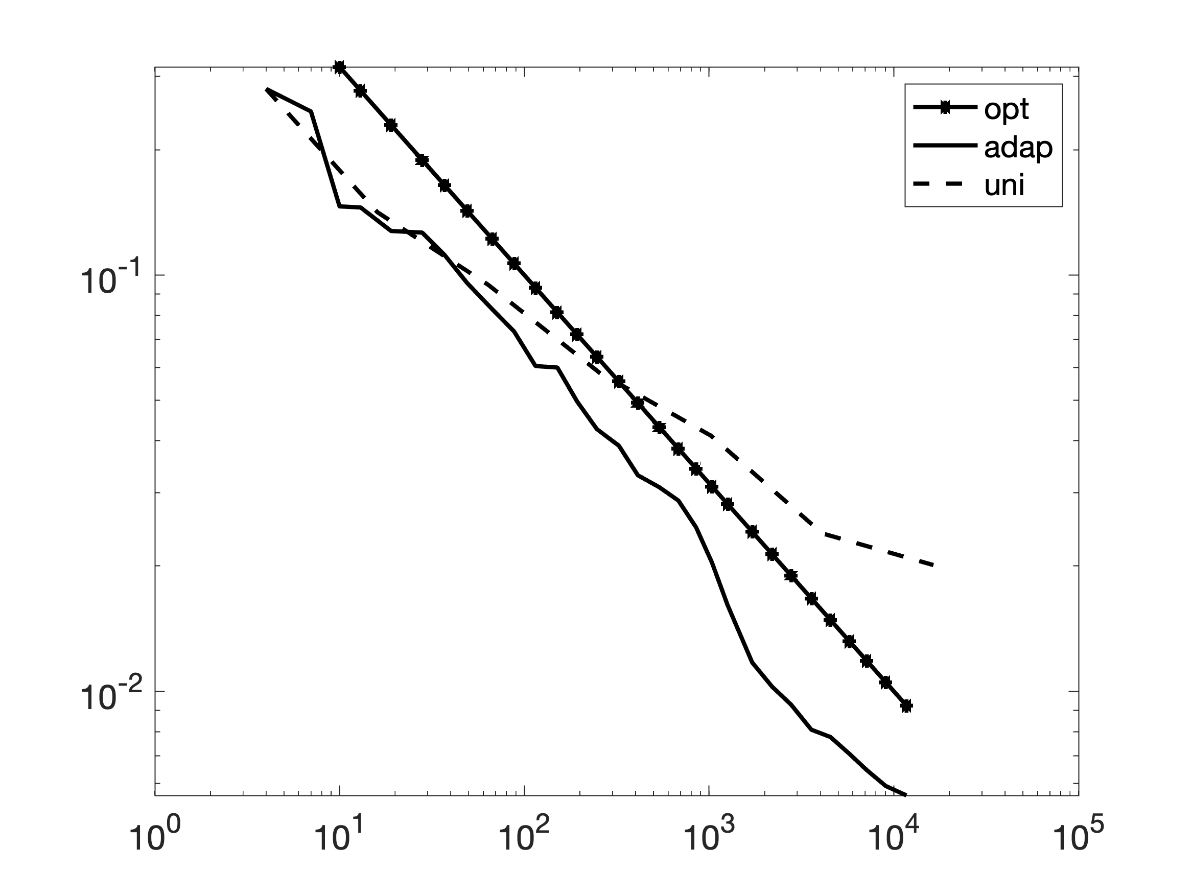
Figure 2 shows the convergence rate for uniformly refined meshes, adaptively refined meshes, and for comparison, the optimal rate $1/\sqrt{N}$ with $N$ denoting the number of elements. We observe that the error for the uniformly refined grids behaves suboptimal, while the error for the adaptively refined grid is nearly parallel to the optimal curve. Here, we adapted the grid by using the local $L^{2}$-error between the numerical solution and the exact solution, i.e., for each $K\in\mathcal{T}$ we use

$$\eta_{K}^{2}=\|u-u_{h}\|_{L^{2}(K)}^{2},$$

which is computed using numerical quadrature; see Figure 2 for an illustration. The mesh is then refined by a Dörfler marking strategy [29], that is all elements in the set $\mathcal{K}\subset\mathcal{T}$ are refined, where $\mathcal{K}\subset\mathcal{T}$ is the set of smallest cardinality such that

$$\sum_{K\in\mathcal{K}}\eta_{K}^{2}>0.3\sum_{K\in\mathcal{T}}\eta_{K}^{2}.$$

An intermediate mesh with $N=151$ elements obtained in this way is shown in Figure 2. We clearly see the local refinement towards the discontinuity of $u$ for $\mu=1/\sqrt{2}$.

Figure 2: Non-smooth test case eq. 14. Top left: Locally refined mesh with local mesh sizes varying from $1/2^{2}$ to $1/2^{6}$ for $N=151$ elements. Top right: Local $L^{2}$-error times the size of an element for the grid shown left. Bottom: Convergence for uniformly refined grids (dotted), adaptively refined grids (connected), and, for comparison, the rate $1/\sqrt{N}$ (connected with stars) for different number of elements $N$ in a double logarithmic scale.

6 Conclusions

We developed and analyzed a discontinuous Galerkin approximation for the radiative transfer equation in slab geometry. The use of quadtree-like grids allowed for a relatively simple analysis with similar arguments as for more standard elliptic problems. While such grids allow for local mesh refinement in phase-space, the implementation of the numerical scheme is straightforward. For sufficiently regular solutions, we showed optimal rates of convergence.

We showed by example that non-smooth solutions can be approximated well by adaptively refined grids. In order to automate the mesh adaptation procedure, an a posteriori error estimator is required. Since the solution to eq. 1–eq. 2 is not in $H^{1}(\Omega)$ and is even allowed to be discontinuous, it seems difficult to generalize residual error estimators for elliptic problems, see, e.g., [10, Section 5.6] or [3, 29]. Upper bounds for the error can be derived for consistent approximations using duality theory [17]. Rigorous a posteriori error estimation has also been done using discontinuous Petrov-Galerkin discretizations [8]. We leave it to future research to investigate the construction of reliable and efficient local error estimators for the DG scheme considered here.

References

- [1] M. L. Adams and E. W. Larsen. Fast iterative methods for discrete-ordinates particle transport calculations. Progress in Nuclear Energy, 40(1):3–159, 2002.
- [2] V. Agoshkov. Boundary Value Problems for Transport Equations. Modeling and Simulation in Science, Engineering and Technology. Birkhäuser, Boston, 1998.
- [3] Mark Ainsworth and J. Tinsley Oden. A posteriori error estimation in finite element analysis. Pure and Applied Mathematics (New York). Wiley-Interscience [John Wiley & Sons], New York, 2000.
- [4] D. Arnush. Underwater light-beam propagation in the small-angle-scattering approximation. Journal of the Optical Society of America, 62(9):1109, sep 1972.
- [5] Susanne C. Brenner and L. Ridgway Scott. The mathematical theory of finite element methods. Springer, 3 edition, 2008.
- [6] T. Burger, J. Kuhn, R. Caps, and J. Fricke. Quantitative determination of the scattering and absorption coefficients from diffuse reflectance and transmittance measurements: Application to pharmaceutical powders. Appl. Spectrosc., 51(3):309–317, Mar 1997.
- [7] Rémi Carminati and John C. Schotland. Principles of Scattering and Transport of Light. Cambridge University Press, jun 2021.
- [8] Wolfgang Dahmen, Felix Gruber, and Olga Mula. An adaptive nested source term iteration for radiative transfer equations. Mathematics of Computation, 89(324):1605–1646, 2020.
- [9] Valmor F De Almeida. An iterative phase-space explicit discontinuous Galerkin method for stellar radiative transfer in extended atmospheres. Journal of Quantitative Spectroscopy and Radiative Transfer, 196:254–269, 2017.
- [10] Daniele Antonio Di Pietro and Alexandre Ern. Mathematical aspects of discontinuous Galerkin methods, volume 69 of Mathématiques & Applications (Berlin) [Mathematics & Applications]. Springer, Heidelberg, 2012.
- [11] J. J. Duderstadt and W. R. Martin. Transport Theory. John Wiley & Sons, Inc., New York, 1979.
- [12] H. Egger and M. Schlottbom. A mixed variational framework for the radiative transfer equation. Math. Mod. Meth. Appl. Sci., 22:1150014, 2012.
- [13] Y Favennec, T Mathew, MA Badri, Pierre Jolivet, Benoit Rousseau, D Lemonnier, and PJ Coelho. Ad hoc angular discretization of the radiative transfer equation. Journal of Quantitative Spectroscopy and Radiative Transfer, 225:301–318, 2019.
- [14] Pascal Jean Frey and Paul-Louis George. Mesh Generation - Applications to Finite Elements. John Wiley & Sons Inc., 2nd edition, 2008.
- [15] David Gilbarg and Neil S. Trudinger. Elliptic partial differential equations of second order. Classics in Mathematics. Springer-Verlag, Berlin, 2001. Reprint of the 1998 edition.
- [16] Jean-Luc Guermond, Guido Kanschat, and Jean C Ragusa. Discontinuous Galerkin for the radiative transport equation. In Recent developments in discontinuous Galerkin finite element methods for partial differential equations, pages 181–193. Springer, 2014.
- [17] Weimin Han. A posteriori error analysis in radiative transfer. Applicable Analysis, 94(12):2517–2534, dec 2014.
- [18] Weimin Han, Jianguo Huang, and Joseph A. Eichholz. Discrete-ordinate discontinuous galerkin methods for solving the radiative transfer equation. SIAM Journal on Scientific Computing, 32(2):477–497, 2010.
- [19] James E. Hansen and Larry D. Travis. Light scattering in planetary atmospheres. Space Science Reviews, 16(4):527–610, oct 1974.
- [20] Gerhard Kitzler and Joachim Schöberl. A high order space–momentum discontinuous Galerkin method for the boltzmann equation. Computers & Mathematics with Applications, 70(7):1539–1554, 2015.
- [21] Daniel Kitzmann, Jan Bolte, and A Beate C Patzer. Discontinuous Galerkin finite element methods for radiative transfer in spherical symmetry. Astronomy & Astrophysics, 595:A90, 2016.
- [22] József Kópházi and Danny Lathouwers. A space–angle DGFEM approach for the Boltzmann radiation transport equation with local angular refinement. Journal of Computational Physics, 297:637–668, 2015.
- [23] LH Liu. Finite element solution of radiative transfer across a slab with variable spatial refractive index. International journal of heat and mass transfer, 48(11):2260–2265, 2005.
- [24] William R Martin and James J Duderstadt. Finite element solutions of the neutron transport equation with applications to strong heterogeneities. Nuclear Science and Engineering, 62(3):371–390, 1977.
- [25] William R Martin, Carl E Yehnert, Leonard Lorence, and James J Duderstadt. Phase-space finite element methods applied to the first-order form of the transport equation. Annals of Nuclear Energy, 8(11-12):633–646, 1981.
- [26] Rustamzhon Melikov, Daniel Aaron Press, Baskaran Ganesh Kumar, Sadra Sadeghi, and Sedat Nizamoglu. Unravelling radiative energy transfer in solid-state lighting. Journal of Applied Physics, 123(2):023103, jan 2018.
- [27] Olena Palii and Matthias Schlottbom. On a convergent DSA preconditioned source iteration for a DGFEM method for radiative transfer. Computers and Mathematics with Applications, 79(12):3366–3377, 2020.
- [28] Jean C Ragusa and Yaqi Wang. A two-mesh adaptive mesh refinement technique for SN neutral-particle transport using a higher-order DGFEM. Journal of computational and applied mathematics, 233(12):3178–3188, 2010.
- [29] Rüdiger Verfürth. A Posteriori Error Estimation Techniques for Finite Element Methods. Oxford University Press, apr 2013.