Rapid generation of all-optical ³⁹K Bose-Einstein condensates using a low-field Feshbach resonance

Abstract

Ultracold potassium is a promising candidate for quantum technology applications and fundamental research as it allows controlling intra-atomic interactions via low-field magnetic Feshbach resonances. However, the realization of high-flux sources of Bose-Einstein condensates remains challenging due to the necessity of optical trapping to use magnetic fields as external degree of freedom. We investigate the production of all-optical ³⁹K Bose-Einstein condensates with different scattering lengths using a Feshbach resonance near $33\text{\,}\mathrm{G}$. By tuning the scattering length in a range between $75\text{\,}\mathrm{a}_{\mathrm{0}}$ and $300\text{\,}\mathrm{a}_{\mathrm{0}}$ we demonstrate a trade off between evaporation speed and final atom number and decrease our evaporation time by a factor of 5 while approximately doubling the evaporation flux. To this end, we are able to produce fully condensed ensembles with $5\text{\times}{10}^{4}\text{\,}\mathrm{a}$toms within $850\text{\,}\mathrm{m}\mathrm{s}$ evaporation time at a scattering length of $232\text{\,}\mathrm{a}_{\mathrm{0}}$ and $1.6\text{\times}{10}^{5}\text{\,}\mathrm{a}$toms within $4\text{\,}\mathrm{s}$ at $158\text{\,}\mathrm{a}_{\mathrm{0}}$, respectively. We deploy a numerical model to analyse the flux and atom number scaling with respect to scattering length, identify current limitations and simulate the optimal performance of our setup. Based on our findings we describe routes towards high-flux sources of ultra-cold potassium for inertial sensing.

I Introduction

Decades after their first experimental realization [1, 2], Bose-Einstein condensates (BEC) have become a central tool in research ranging from many-body physics [3] to quantum technology applications such as computation [4], simulation [5], and sensing and metrology [6]. High-flux sources of Bose-Einstein condensates have always been of particular interest, especially with respect to signal-to-noise ratios and quantum projection noise.

To this end, the state-of-the-art has been established by sources based on atom chips [7, 8] as demonstrated in the scope of compact apparatuses for microgravity experiments [9, 10, 11, 12] and as chosen for current and planned experiments in orbit on the ISS [13, 14]. Here, forming traps near the current-conducting structures allows generating strongly confining traps and hence rapid and efficient evaporation. Likewise, the nearby surface of the atom chip may sometimes be considered unfavorable, e.g., with respect to clipping of atom optics light fields or, in presence of notable temperature gradients, due to black-body radiation [15]. In an alternative approach, Bose-Einstein condensation has been demonstrated in all-optical setups [16, 17, 18, 19] capable of trapping any magnetic substate. With the ability to focus optical dipole trap beams into the center of the experimental apparatus, generally this leaves a larger clear aperture for optical access as compared to atom chip solutions [20, 21]. Moreover, recent studies have shown a variety of tools to counteract the typical scaling laws when evaporatively cooling in optical traps [22], e.g., by movable lens systems [23] or dynamically shaped time-averaged potentials [24, 25, 26]. Finally, while trapping any substate irrespective of whether high or low magnetic field seeking, with the external magnetic field as a free parameter optical traps offer ideal conditions for studying and utilizing Feshbach resonances [27, 28]. As a versatile means of tailoring interactions, Feshbach resonances have for instance enabled the production of cold molecules from a Fermi gas [29, 30], molecular BECs [31, 32, 33], sympathetic cooling [34, 35], ground-state molecules [36] and studies of interaction dynamics [37, 38]. Finally, for cooling fermionic species, Feshbach-induced collisions have been proposed and demonstrated as a evaporation knife [39, 40].

In this work, we demonstrate rapid evaporation of ³⁹K gases to quantum degeneracy from a time-averaged optical trap. By using low-field Feshbach resonances [41, 18, 42] we are able to directly tune the rethermalization rate and show a linear dependence between evaporation flux in the BEC and the scattering length when sufficiently distant from the resonance. Accordingly, compared to the largest prepared BEC we are able to decrease our evaporation time by a factor of 5 while approximately doubling the evaporation flux when tuning the scattering length. We describe our apparatus and the detailed experimental sequence including direct loading of the optical trap and a multi-stage magnetic state preparation. We finally discuss the prospects of using our result in compact quantum inertial sensors using tunable interactions.

II Experimental setup

Figure 1: a) Layout of the laser system for D₁-cooling: The external cavity laser (ECDL) is stabilized via modulation transfer spectroscopy to the $\ket{F=1/2}\rightarrow\ket{F^{\prime}=1/2}$ crossover transition. The double-pass AOM (AOM2) shifts the laser’s frequency to match the D₁ cooling transition before passing the amplifier (TA). Optical isolators (OI) are used to prevent potential back-reflections into TA and ECDL. The free space EOM creates the repump light. The subsequent AOM (AOM3) allows for fast amplitude switching. b) Optical dipole trap layout: The laser beam is focused, re-collimated, redirected and focused again through the vacuum chamber by three lenses (L) with a focal length of $150\text{\,}\mathrm{mm}$. To suppress heating effects the linear polarization of the laser is $90\text{\,}\mathrm{\SIUnitSymbolDegree}$ rotated by $\lambda/2$ retardation plates (HWP) and cleaned up by two laser polarizers (Pol.), which are oriented orthogonal to each other. A Yagi-Uda micro-wave antenna (MWA) is used for coherent manipulation of the atoms. Quantization coil pairs are aligned with the depicted coordinate system, while the Feshbach fields are generated by another Helmholtz pair along the y-axis. The detection (purple arrow) is performed under an angle of $14°$ in respect to the y-axis.

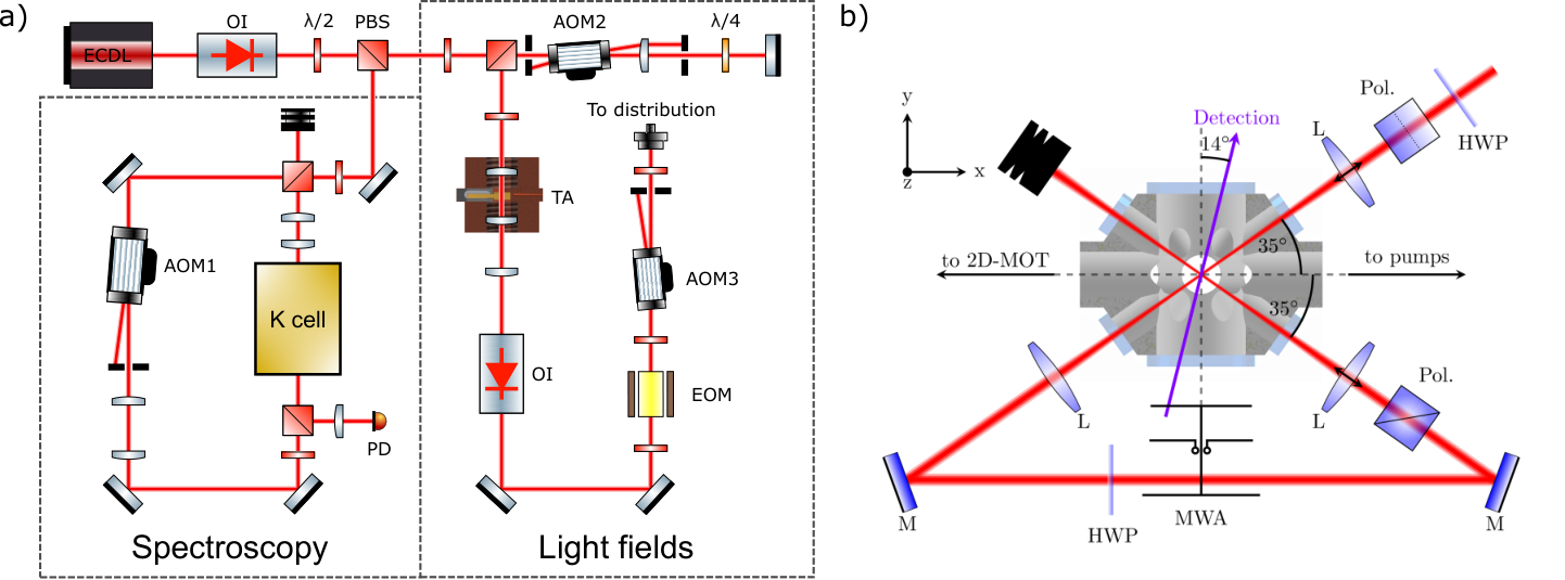
II.1 Laser system

Trapping and cooling of potassium is performed using transitions on both the D₁- and D₂-line. The D₂-laser system and its performance have been described previously [43, 44]. In this work we additionally operate a laser system on the D₁-line (Fig. 1a). To this end, $5\text{\,}\mathrm{m}\mathrm{W}$ of an external cavity diode laser’s [45, 46] output are used for frequency stabilization to the potassium D₁-crossover line $\ket{F=1/2}\rightarrow\ket{F^{\prime}=1/2}$ in a vapour cell by means of modulation transfer spectroscopy [47]. The remaining $30\text{\,}\mathrm{m}\mathrm{W}$ are frequency shifted by a double-pass AOM to match the D₁ cooling transition $\ket{F=2}\rightarrow\ket{F^{\prime}=2}$ which has an offset of $152.3\text{\,}\mathrm{MHz}$ with respect to the crossover transition. Subsequently, the light is amplified by a tapered amplifier [Eagleyard EYP-TPA-0765-01500-3006-CMT03-0000] yielding a total output power of $1000\text{\,}\mathrm{mW}$. The repump transition $\ket{F=1}\rightarrow\ket{F^{\prime}=1}$ is addressed using a side band generated by a resonant free-space EOM [Qubig PM-K39+41] driven with a maximum input power of $31.7\text{\,}\mathrm{d}\mathrm{B}\mathrm{m}$, allowing one to freely tune the power ratio between carrier and side band in a range from $0$ to $1$. The cooling and repumping fields are then transported via a polarization-maintaining fiber [S&K PMC-E-630-4.1-NA012-3-APC.EC-1000-P] with $60\text{\,}\%$ coupling efficiency yielding $500\text{\,}\mathrm{m}\mathrm{W}$ in total at the fiber output. Finally, the fiber output is superimposed with the D₂-light using a narrow-line interference filter and launched downstream towards the power distribution module.

II.2 Optical dipole trap

Our optical dipole trap is based on a $1960\text{\,}\mathrm{nm}$ fiber laser [IPG, TLR-50-1960-LP] operated at $38\text{\,}\mathrm{W}$ output power. The lasers intensity is stabilized by a FPGA feedback loop controlling and linearizing a Pockels cell and analyzer setup. We focus an elliptical beam in the vacuum chamber with a beam waist of 30(45) $\mathrm{\SIUnitSymbolMicro m}$ in horizontal (vertical) direction and realize a recycled cross under an angle of $70\text{\,}\mathrm{\SIUnitSymbolDegree}$ (Fig. 1b) with a maximum power of $8\text{\,}\mathrm{W}$ in the primary and $6\text{\,}\mathrm{W}$ in the secondary beam. By modulating the center-position of the laser beams we generate time-averaged potentials in the horizontal plane using an acousto-optical modulator [24, 26, 48]. With this we can reach trap depths from $U_{0}=$ $130\text{\,}\mathrm{nK}$ to $530\text{\,}\mathrm{\SIUnitSymbolMicro K}$, corresponding to trapping frequencies of $\omega/2\pi=\{4;6;50\}$ $\mathrm{Hz}$ to $\{1.3;1.9;2.2\}$ $\mathrm{kHz}$ in $\{x;y;z\}$-direction.

II.3 Magnetic field control

The coil setup creating the magnetic fields consists of three Helmholtz pairs oriented along the coordinate system in figure 1b and the main coil pair along the y-axis. The former are used to define the quantization axes during state preparation and imaging as well as for compensating stray magnetic fields ($\left|B_{x,y,z}\right|\leq$$1\text{\,}\mathrm{G}$) during cooling and trapping. The stabilization electronics allow for two different operation modes. In presence of the MOT- and Feshbach magnetic fields the system is stabilizing the current, utilizing current transducers [LEM CASR 15-NP]. During the state preparation the magnetic fields are directly stabilized using a three-axis fluxgate sensor [Bartington MAG-03IE1000] mounted close to the vacuum chamber giving us a relative short-term stability of $\sigma=\left\{15;\,16;\,6.6\right\}\cdot 10^{-4}$ in $\left\{\text{x; y; z}\right\}$-direction at $\tau=$$10\text{\,}\mathrm{ms}$.

The main coils can be operated in Helmholtz and anti-Helmholtz configuration providing the homogeneous magnetic field for tuning the interaction strength during evaporation and the gradient magnetic fields (characterization see [49]) in the laser cooling stages. To switch between these configurations a home build H-bridge, based on mosfets [IXYS 747-IXFN170N65X2] with a low drain-source on-resistance of $13\text{\,}\mathrm{m\SIUnitSymbolOhm}$ is used. The coils are driven in series by one power supply [EA-PSI 9200-25] with a maximum voltage of $200\text{\,}\mathrm{V}$ limiting the current to $11.1\text{\,}\mathrm{A}$ due to the coils internal resistance ($18\text{\,}\mathrm{\SIUnitSymbolOhm}$). For current stabilization the internal stabilization loop is used allowing for a current stability of $<0.15\text{\,}\%$. For characterizing the applied magnetic field at the position of the atoms we determine the positions of several known Feshbach resonances with respect to coil current by observing the enhancement of atom losses close to the resonance [50, 51]. We find the six resonances expected [41, 52] (table 1) for a mixture of $\ket{F=1,m_{F}=-1}$ and $\ket{F=1,m_{F}=0}$ at $15\text{\,}\mathrm{\SIUnitSymbolMicro K}$ below $200\text{\,}\mathrm{G}$. Applying a Biot-Savart model of our setup yields $41.2\text{\,}\mathrm{G}$ with a maximum magnetic field strength of $450\text{\,}\mathrm{G}$ and an accuracy of $0.2\text{\,}\mathrm{G}$.

Table 1: Identified Feshbach resonances, used to calibrate the magnetic fields. The magnetic field values are taken from [52].

			Measured	Literature
Atom pair ($F,m_{F}$)			current (A)	magnetic field (G)
$(1,-1)$	$+$	$(1,-1)$	$0.795\pm 0.002$	$32.6\pm 1.5$
$(1,0)$	$+$	$(1,0)$	$1.450\pm 0.003$	$59.3\pm 0.6$
$(1,0)$	$+$	$(1,0)$	$1.600\pm 0.003$	$66.0\pm 0.9$
$(1,0)$	$+$	$(1,-1)$	$2.762\pm 0.006$	$113.76\pm 0.1$
$(1,-1)$	$+$	$(1,-1)$	$3.968\pm 0.008$	$162.8\pm 0.9$

III Quantum gas production

In the following we detail the dipole trap loading sequence (Fig. 2a), the magnetic substate preparation (Fig. 2b), and the evaporative cooling procedure.

III.1 Loading sequence

Figure 2: a) Loading scheme of the optical dipole trap: We initially load a MOT on the D₂ line from a 2D-MOT. Afterwards we use a Hybrid D₁-D₂ compressed MOT to increase the peak density while cooling the ensemble simultaneously. Subsequently sub-Doppler temperatures of $12\text{\,}\mu\mathrm{K}$ are achieved by D₁ gray molasses cooling. This scheme allows to directly load the ODT, without the need for magnetic trapping as intermediate step. b) State preparation loop within the optical dipole trap: A combination of coherent microwave transfers and optical pumping is used to shift the population towards $m_{F}=-1$, starting from a equally populated mixture in $F=1$. A blow-away sequence is added at the end to increase the purity of the ensemble. After 4 loops, each $70\text{\,}\mathrm{ms}$ long, we reach an almost pure ensemble ($>$98%) with a temperature increase of $~0.3\text{\,}\mathrm{\SIUnitSymbolMicro K}$ per loop.

Initially, we load $1\text{\times}{10}^{9}$ atoms in a 3D magneto-optical trap (MOT) within $4\text{\,}\mathrm{s}$ from a beam formed by a 2D-MOT. Afterwards we switch off the D₂ cooling light and simultaneously turn on the D₁ cooling light field, thus enabling a D₁ gray molasses dipole trap loading scheme [53]: By ramping up the magnetic field gradient from $4\text{\,}\mathrm{G}\mathrm{/}\mathrm{c}\mathrm{m}$ to $15\text{\,}\mathrm{G}\mathrm{/}\mathrm{c}\mathrm{m}$ and the D₂ repumping light down to 0.25 I${}_{\text{sat}}$ we perform a hybrid D₁-D₂ compressed MOT, to increase the density and simultaneously cool the ensemble to below $200\text{\,}\mathrm{\SIUnitSymbolMicro K}$ within $16\text{\,}\mathrm{ms}$. We then switch off the remaining D₂ repumping light and the magnetic field gradient to perform gray molasses cooling, resulting in a final temperature of $12\text{\,}\mathrm{\SIUnitSymbolMicro K}$ after $40\text{\,}\mathrm{ms}$. With the optical dipole trap already turned on at the maximum available power and a center-position modulation amplitude of $160\text{\,}\mathrm{\SIUnitSymbolMicro m}$ during the MOT loading and cooling sequence we load a total of $12\text{\times}{10}^{6}$ atoms into the trap, corresponding to a transfer efficiency of $2\text{\,}\%$, with $3\text{\times}{10}^{6}$ atoms positioned in the beams’ crossing region.

III.2 State preparation

Upon loading the dipole trap we depump the atomic ensemble into $\ket{F=1}$ by shining in $1\text{\,}\mathrm{mW}$ of D₁ cooling light with a detuning of $-1\text{\,}\Gamma$ via the detection optics, thus creating an equidistributed $m_{F}$-mixture. To generate a spin-polarized ensemble in $\ket{F=1,m_{F}=-1}$, we then utilize a multi-loop state preparation scheme [54] combining optical pumping on the D₁-line with microwave adiabatic rapid passages driven by a Yagi-Uda-type directed antenna. We initially apply a quantization field of $0.7\text{\,}\mathrm{G}$ at an angle of $45\text{\,}\mathrm{\SIUnitSymbolDegree}$ to the antenna’s Poynting vector oriented in the horizontal plane. This allows us to transfer the population of $\ket{F=1,m_{F}=0}$ to $\ket{F=2,m_{F}=0}$ by driving a $\pi$-transition sweeping the microwave from $461.710\text{\,}\mathrm{MHz}$ to $461.730\text{\,}\mathrm{MHz}$ within $4\text{\,}\mathrm{ms}$. We subsequently apply $\sigma^{-}$-polarized D₁ cooling light via the detection optics with a detuning of $-5\text{\,}\Gamma$ for $2\text{\,}\mathrm{ms}$ in order to depump the atoms into $\ket{F=1}$ via spontaneous emission, hence populating $\ket{F=1,m_{F}=0}$ and $\ket{F=1,m_{F}=-1}$. Due to the mismatch of quantization field axis and detection beam orientation by $14\text{\,}\mathrm{\SIUnitSymbolDegree}$ we also drive the $\ket{F=2,m_{F}=-2}\rightarrow\ket{F^{\prime}=2,m_{F}=-2}$ transition, thus preventing accumulation in $\ket{F=2,m_{F}=-2}$. We then rotate the magnetic field axis to be parallel to the antenna’s Poynting vector by tuning the vertical field component to zero, effectively resulting in an quantization field in the horizontal plane of $0.5\text{\,}\mathrm{G}$. In this configuration we are able to drive a $\sigma$-polarized microwave adiabatic rapid passage. Sweeping from $462.062\text{\,}\mathrm{MHz}$ to $462.080\text{\,}\mathrm{MHz}$ in $12\text{\,}\mathrm{ms}$ we transfer atoms from $\ket{F=1,m_{F}=+1}$ to $\ket{F=2,m_{F}=0}$. Due to the symmetry of the level structure the same microwave pulse also drives the unwanted transition from $\ket{F=1,m_{F}=0}$ to $\ket{F=2,m_{F}=-1}$. However, since $\ket{F=1,m_{F}=0}$ has already been addressed with the first pulse fewer atoms are available for undesired transitions. We afterwards apply the same optical depumping pulse as before, thus transferring the atoms back into $\ket{F=1}$. While this sequence does not yield a pure magnetic substate, it shifts the $m_{F}$-distribution towards $m_{F}=-1$. Repeating the sequence multiple times allows us to accumulate atoms in $\ket{F=1,m_{F}=-1}$. As a final step, we purify the ensemble by a blowaway sequence: We apply the same microwave pulses as before but tune the D₁ cooling laser closer to resonance ($-1\text{\,}\Gamma$) to purposely heat atoms out of the trap during optical pumping.

By performing four loops as described we reach an almost pure ensemble ($>98\text{\,}\%$ in $\ket{F=1,m_{F}=-1}$) with $70\text{\,}\%$ of the initial atoms remaining in the trap. Since the D₁-line does not feature closed transitions, with $~0.3\text{\,}\mathrm{\SIUnitSymbolMicro K}$ per loop the observed heating due to the state preparation sequence is minimal and yields a final temperature of $9.6\text{\,}\mathrm{\SIUnitSymbolMicro K}$.

III.3 Feshbach resonances & evaporation

To address Feshbach resonances we generate homogeneous magnetic fields by switching the MOT magnetic field coils from anti-Helmholtz to Helmholtz configuration. We then ramp up the magnetic field to the desired value in $100\text{\,}\mathrm{ms}$. The corresponding scattering length close to the resonances can be calculated using the background scattering length $a_{\text{bg}}$, the resonance widths $\Delta_{i}$ and its center $B_{0i}$ [55, 41]:

$$a(B)=a_{\text{bg}}\left(1-\sum_{i}\frac{\Delta_{i}}{B-B_{0i}}\right)$$ (1)

Once a stable final magnetic field and thus atomic scattering length is established we use the dipole trap’s intensity stabilization in combination with the AOM to piecewise decrease the trap power in five linear ramps. In parallel, the center-position modulation (CPM) is rampd down and reaches zero with the final ramp at the end of the evaporation sequence. The initial center-position modulation amplitude is determined by the optimal mode match for trap loading. We optimize each step with respect to the final atom number in the BEC by tuning the intensity reduction, the CPM amplitude reduction, and the ramp lengths as free parameters.

IV Experimental results

Figure 3: a) BEC size and time dependency with respect to scattering length: The largest fully condensed BEC is realized at a scattering length of $158\text{\,}\mathrm{a}_{\mathrm{0}}$ (blue square). For lower and higher scattering lengths the final atom number is reduced. The inlay shows the time needed for evaporating. For higher scattering lengths the higher elastic collision rates allow for faster evaporation resulting in a smaller time constant. The fastest BEC is realized at a scattering length of $232\text{\,}\mathrm{a}_{\mathrm{0}}$ (red diamond) with a total evaporation time of $850\text{\,}\mathrm{ms}$. b) Flux of the evaporative cooling against scattering length: For the fully optimized ramps we find the flux to scale linearly with the scattering length. The highest flux is achieved at a scattering length of $232\text{\,}\mathrm{a}_{\mathrm{0}}$. c) Phase space density trajectory for largest BEC and highest flux: For the evaporation efficiency $\gamma$ only the data points on the ramp and not the starting point are taken into account. We find equal efficiency for both cases but deteriorated initial conditions at $232\text{\,}\mathrm{a}_{\mathrm{0}}$, resulting in a lower final atom number.

We systematically optimize BEC production for different scattering lengths (Fig. 3a). Initially, we optimize the ramp itself. In accordance with [24] we find our evaporation sequence to be most efficient using an exponential reduction for the trap power jointly with a linear reduction slope for the center-position modulation amplitude. We achieve a fully condensed BEC of $1.3\text{\times}{10}^{5}$ atoms at a scattering length of $158\text{\,}\mathrm{a}_{\mathrm{0}}$ after evaporating over the course of $3.9\text{\,}\mathrm{s}$. While our setup allows to dynamically tune to different scattering lengths during each of the five ramps, we did not observe significant beneficial effects on the final atom number in the BEC. To analyse the scaling behaviour with respect to scattering length, we additionally optimize the BEC size at lower and higher scattering length (Fig. 3, orange circles), by re-scaling the overall length of evaporation ramp while maintaining its shape. At a lower scattering length the final atom number is reduced while the time needed for evaporation is increased, due to the reduced elastic collision rate stretching the length of the overall sequence. At scattering lengths $\leq 75\text{\,}\mathrm{a}_{\mathrm{0}}$ we are unable to reach condensation as we are limited by the lifetime of our optical dipole trap, which we measured to be $15\text{\,}\mathrm{s}$. For scattering lengths $>158\text{\,}\mathrm{a}_{\mathrm{0}}$ we find a reduced final atom number, as well. However, the higher elastic collision rate now allows one to significantly reduce the time needed for evaporation. We experimentally find a limit for this trade off at $>300\text{\,}\mathrm{a}_{\mathrm{0}}$ were we are unable to reach condensation. Based on the initial findings we individually alter the relative length of the five linear ramps towards the globally largest BEC size and the largest BEC size at the shortest evaporation time possible. Globally, we find a maximum atom number of $1.6\text{\times}{10}^{5}$ in the BEC at $158\text{\,}\mathrm{a}_{\mathrm{0}}$, close to the initial configuration and with the same total ramp length (Fig. 3, blue square). Our fastest evaporation is performed within $850\text{\,}\mathrm{ms}$ at a scattering length of $232\text{\,}\mathrm{a}_{\mathrm{0}}$ yielding a fully condensed BEC of $5\text{\times}{10}^{4}$ atoms (Fig. 3, red diamond). Compared to the trajectory at $158\text{\,}\mathrm{a}_{\mathrm{0}}$ this corresponds to a reduction in evaporation time by a factor of 5 while approximately doubling the evaporation flux, which we define as final atom number in the condensate over evaporation time  (Fig. 3b). For scattering lengths in the range of $75\dots\,232\text{\,}\mathrm{a}_{\mathrm{0}}$ and optimized ramps we observe a linear relation between scattering length and evaporation flux.

We perform a detailed analysis of both trajectories, measuring atom number and temperature after each linear ramp and adapting a simulation to them as described in the appendix. For the phase space density $\rho$ we find the evaporation efficiency $\gamma=-\frac{d\ln(\rho)}{d\ln(N)}$ to be the same for both cases due to the individual optimization (Fig. 3c) but with worse initial conditions at $232\text{\,}\mathrm{a}_{\mathrm{0}}$. Losses from evaporation increase by an order of magnitude at $232\text{\,}\mathrm{a}_{\mathrm{0}}$ (Fig. 4a), from which a factor of two is explained by the higher scattering length due to the corresponding $a^{2}$-scaling [56]. Based on equation (7) the remaining factor of five is linked to the reduction of the truncation factor $\eta$ (Fig. 4b), corresponding to an initial reduction in energy removal per scattering event by a factor of 2. At $232\text{\,}\mathrm{a}_{\mathrm{0}}$ we additionally expect an increase in three body losses by a factor of five compared to $158\text{\,}\mathrm{a}_{\mathrm{0}}$, due to the underlying $a^{4}$-scaling [50]. However, this effect is compensated by the lower peak density along the trajectory (Fig. 4c). Therefore, a more favorable ratio of good to bad collisions is realized at $232\text{\,}\mathrm{a}_{\mathrm{0}}$, allowing to speed up the evaporation, without reducing the evaporation efficiency. To this end the final atom number is limited by the initial conditions and the corresponding low $\eta$ at the beginning of the evaporation. This behaviour is already apparent in the phase space diagram (Fig. 3c) were the initial phase space density does not match the fitted efficiency curve. Indeed, using the initial conditions from the trajectory at $158\text{\,}\mathrm{a}_{\mathrm{0}}$ our simulation yields a final atom number of $>1\text{\times}{10}^{5}$ for the $232\text{\,}\mathrm{a}_{\mathrm{0}}$-trajectory with losses as expected from their respective scaling behaviour.

Figure 4: Underlying mechanisms of the evaporation trajectories at $158\text{\,}\mathrm{a}_{\mathrm{0}}$ (bounded by solid blue lines) and $232\text{\,}\mathrm{a}_{\mathrm{0}}$ (bounded by dashed red lines) resulting from the simulation as described in the appendix; The bands represent the outcome for all possible three-body loss scaling factors $C(a)$ as defined in [24, 50]. a) Loss rates from evaporative cooling: At $232\text{\,}\mathrm{a}_{\mathrm{0}}$ the evaporation rate is enhanced by an order of magnitude, with a factor of two originating from the higher scattering length and a factor of 5 due to the lower $\eta$. b) Truncation factor $\eta$: Along similar ramps, the dynamic evolution is entirely determined by the initial conditions. Due to the lower initial density at $232\text{\,}\mathrm{a}_{\mathrm{0}}$, $\eta$ is initially reduced by a factor of approximately 2. c) Loss rates from three-body collisions: While the increase in scattering length in principle corresponds to a five times higher loss rate at $232\text{\,}\mathrm{a}_{\mathrm{0}}$, this effect is compensated by the smaller peak density.

V Conclusion & outlook

V.1 Further enhancement of atomic flux

State-of-the-art atomic sources generate an evaporation flux of $\geq$2\text{\times}{10}^{5}\text{\,}{\mathrm{s}}^{-1}$$ with experimental repetition rates of $\sim$$1\text{\,}\mathrm{Hz}$ for atom interferometry applications utilizing ⁸⁷Rb [7]. Using ³⁹K an evaporation flux of $2.4\text{\times}{10}^{5}\text{\,}{\mathrm{s}}^{-1}$ has been demonstrated in a hybrid setup with a magnetic trap as intermediate step, requiring a magnetic field gradient of $270\text{\,}\mathrm{G}$ and an extended experimental cycle time of $15\text{\,}\mathrm{s}$ [18]. All-optical cooling allows for shorter cycle times and a simplified apparatus with respect to the generation of magnetic fields. In our setup, the current density necessary for generating $1\text{\,}\mathrm{G}\mathrm{/}\mathrm{c}\mathrm{m}$ gradient in anti-Helmholtz configuration generates $\sim$$20\text{\,}\mathrm{G}$ when switched to Helmholtz configuration, thus putting the low-field Feshbach resonances in ³⁹K readily in reach with standard quadrupole field coils as used for laser cooling. For ³⁹K an experimental cycle time of $7\text{\,}\mathrm{s}$ has previously been reported [42] yielding an evaporation flux of $\sim$$1\text{\times}{10}^{4}\text{\,}{\mathrm{s}}^{-1}$ with a final atom number of $2\text{\times}{10}^{4}$ in the pure condensate. At $232\text{\,}\mathrm{a}_{\mathrm{0}}$ ($158\text{\,}\mathrm{a}_{\mathrm{0}}$) we improve on this result by a factor of $\sim$$7$ ($\sim$$4$) in evaporation flux and $\sim$$3$ ($\sim$$8$) in atom number with a cycle time of $6\text{\,}\mathrm{s}$ ($9\text{\,}\mathrm{s}$). As discussed in the previous section, our results can be further improved by means of mode-match optimization yielding a higher initial phase space density.

Finally, to extrapolate the theoretical limit of our setup we perform additional simulations neglecting experimental imperfections, such as thermal lensing effects. The optical potential is generated by two identical beams with initial power $P_{0}=$ $8\text{\,}\mathrm{W}$, a vertical waist of $50\text{\,}\mathrm{\SIUnitSymbolMicro m}$, a horizontal waist of $28\text{\,}\mathrm{\SIUnitSymbolMicro m}$ and ideally overlapping foci, trapping $3\text{\times}{10}^{6}$ atoms with a temperature of $10\text{\,}\mathrm{\SIUnitSymbolMicro K}$ in the crossing region. Evaporation trajectories are defined by an exponential power and linear CPM amplitude reduction and simulated for a given scattering length on a two dimensional grid given by evaporation time $t_{f}$ and final beam power $P(t_{f})=P_{f}$. The simulation is aborted once a BEC fraction $>90\text{\,}\mathrm{\%}$ is estimated via the relation

$$\frac{N_{c}}{N}=1-\left(\frac{T}{T_{c}}\right)^{3}$$ (2)

and atom number and evaporation time are adjusted accordingly. Similar to the experiment we analyse the results with the highest evaporation efficiency. By scaling linearly with the scattering length (Fig. 6), the model predicts the same behaviour as observed experimentally. A peak atom number of $3.5\text{\times}{10}^{5}$ is reached at $125\text{\,}\mathrm{a}_{\mathrm{0}}$ after $3.5\text{\,}\mathrm{s}$ of cooling. Towards higher scattering lengths the final atom number declines due to the reduced ratio of good to bad losses, necessitating additional evaporative cooling. A peak flux of $2.31\text{\times}{10}^{5}\text{\,}{\mathrm{s}}^{-1}$ is reached at $325\text{\,}\mathrm{a}_{\mathrm{0}}$, allowing for a final atom number of $1.5\text{\times}{10}^{5}$ after $640\text{\,}\mathrm{ms}$. Under optimal conditions we thus find the extrapolated flux to be competitive with results achieved in hybrid traps [18]. Notably, when taking more inefficient trajectories with lower final atom number into account even higher fluxes are accessible.

In our setup, the overall cycle time is limited by the MOT loading. By using more sophisticated techniques such as a 2D⁺-MOT design [57, 18] or even cryogenic buffer-gas beam sources [58], we expect to improve our repetition rates towards $\geq$$1\text{\,}\mathrm{Hz}$, enabling a new generation of ³⁹K optical dipole traps on par with the current performance of ⁸⁷Rb chip traps.

Figure 5: Extrapolated performance, simulated for ideal experimental conditions: For each data point 2000 evaporation trajectories are evaluated. Similar to the experimental optimization, the results for the trajectory yielding the highest final atom number are depicted. Qualitatively, we find the same behaviour as observed in the experiment with improved numbers.

Figure 6: Modelling of the scattering length with respect to magnetic field: Low-field Feshbach resonances with parameters from [52] for $\ket{1,-1}+\ket{1,-1}$ (solid line) and $\ket{1,0}+\ket{1,0}$ (dashed line), according to equation (1). At $54.3\text{\,}\mathrm{G}$ both resonances share the same scattering length (dot), allowing to easily transfer a BEC via radio frequency adiabatic rapid passages between both states.

Since the increase of evaporation flux in the BEC only depends on the accessibility of sufficiently broad Feshbach resonances this scheme could also be utilized for different elements. Potentially useful Feshbach resonances are found for ⁸⁷Rb (at $\sim$1007\text{\,}\mathrm{G}$$ with $\Delta=$0.17\text{\,}\mathrm{G}$$) [59], ⁸⁵Rb (at $\sim$155\text{\,}\mathrm{G}$$ with $\Delta=$11.6\text{\,}\mathrm{G}$$) [60] and ²³Na (at $\sim$90\text{\,}\mathrm{G}$$ with $\Delta=$1\text{\,}\mathrm{G}$$) [61], but are subject to individual challenges regarding their width and absolute field magnitude.

V.2 Application to atom interferometry

To apply our methods to atom interferometry a magnetically insensitive population in $m_{F}=0$ is desired. This can be accomplished by transferring atoms into $m_{F}=0$ prior to evaporation which can then be performed in the vicinity of the low-field resonance at $59.3\text{\,}\mathrm{G}$ (Fig. 6). However, the more narrow shape of the resonance requires to operate at a magnetic field of $58.56\text{\,}\mathrm{G}$ with an instability below $20\text{\,}\mathrm{mG}$. This corresponds to an improvement by a factor of $5$ in order to achieve the same scattering length stability as in the present experiment. Alternatively, the atoms can be transferred from $m_{F}=-1$ to $m_{F}=0$ via a radio frequency adiabatic rapid passage. After producing the BEC in $m_{F}=-1$ we propose to sweep the magnetic field to $54.3\text{\,}\mathrm{G}$ where both $m_{F}$-states share the same scattering length (Fig 6), allowing to transfer the atoms with an radio frequency sweep over the resonance at $\sim$$39\text{\,}\mathrm{MHz}$.

We envisage applications in trapped atom interferometry for inertial sensing under exploitation of tunable interactions [62] to enhance coherence times [63]. Moreover, using time-averaged potentials for entanglement via one-axis twisting dynamics [64] or delta-kick squeezing techniques [65] adapted to trapped interferometry, magnetically insensitive spinor BECs close to a Feshbach resonance pave the way for overcoming the standard quantum limit.

Figure 7: a)/b) Trap frequency characterization: Measurements are taken by means of parametric heating for variable beam power without center position modulation and for variable center position modulation at $12\text{\,}\mathrm{W}$ primary beam power. The data points are grouped by their respective magnitude (circle $>$ square $>$ diamond) corresponding to the trap frequencies along the three eigenvectors of the system. The trap model is adapted such that the simulated frequencies (solid $>$ dashed $>$ dotted) match the measured ones in both cases simultaneously. c) Corrected trap frequency and depth for the ramp at $158\text{\,}\mathrm{a}_{\mathrm{0}}$: During evaporation the power reduction causes a focus shift due to thermal lensing which is not covered by the static characterization. To simulate the evaporation trajectories the model is corrected accordingly, using an additional time-dependent exponential factor

Figure 8: Simulated evaporation trajectories for $158\text{\,}\mathrm{a}_{\mathrm{0}}$ (a) and $232\text{\,}\mathrm{a}_{\mathrm{0}}$ (b): Measured points are depicted in black, while the bands span all possible outcomes of the simulation for $C(a)$ in the range $16.84$…$67.12$ according to equation (8).

Appendix A Theoretical modelling

To analyse the scaling behaviour of final atom number and flux we use a theoretical model capable of reproducing our experimental performance. Initially, we determine our trap depth and frequency by modelling our optical dipole trap. The results are used to simulate time evolution of atom number and temperature during evaporation.

A.1 Trap depth & frequencies

Modelling the evaporation depends on the knowledge of trap depth and frequencies along the evaporation trajectory. Here we adapt a numerical model to the initial characterization of our trap to simulate these parameters for arbitrary trap configurations with potentials as derived in detail in Refs. [66, 48, 24]. The potential of a single beam pointing in x-direction is

$$U_{\text{beam}}(x,y,z)=U_{\text{beam},0}\frac{\omega_{0,y}\omega_{0,z}}{\omega_{y}(x)\omega_{z}(x)}I(x,y,z)\,,$$ (3)

taking the beam’s ellipticity as well as corresponding focus point shifts via the beam waists $\omega_{i}(x)$ into account. Horizontal center-position modulation is described with the intensity distribution:

$$\begin{gathered}I(x,y,z)=\frac{2P}{\pi\omega_{y}(x)\omega_{z}(x)}\frac{1}{\sum_{i}g(y_{i})}\\ \times\sum_{i}g(y_{i})\exp\left({\frac{-2(y-y_{i})^{2}}{\omega_{y}(z)^{2}}}\right)\exp\left({\frac{-2z^{2}}{\omega_{z}(x)^{2}}}\right)\,,\end{gathered}$$ (4)

realizing an envelop defined by the harmonic potential $g(y_{i})=1-(y_{i}/h)^{2}$ with width $2h$. The spacing of $y_{i}$ is chosen such that the simulation time is minimized without affecting the resulting shape. The full potential is build by rotating and shifting the coordinate system of two beams into our lab frame and adding the gravitational potential $U_{trap}(x,y,z)=U_{beam1}(x_{1},y_{1},z_{1})+U_{beam2}(x_{2},y_{2},z_{2})+mgz$. By changing the individual coordinate transformation, experimental imperfections regarding the angle between both beams, focus position and possible tilts are taken into account. The trap minimum is determined numerically as the local minimum of the potential in the crossing region. In this point we simulate the trap frequencies along the principle axes by determining the eigenvalues of the hessian matrix and the trap depth by taking the difference in potential between local minimum and maximum in z-direction. The free parameters of the model are adjusted by matching the simulated to measured trap frequencies. Measurements are taken for variable power without center-position modulation (Fig. 7a) and for variable CPM amplitude with constant power. (Fig. 7b) For each measurement we statically load the dipole trap from the molasses in the desired configuration. Afterwards we measure the trap frequencies along the principle axes by parametric heating. The resulting model is used to simulate the trap behaviour on a grid spanning all possible power and painting stroke configurations. In between points missing values are interpolated using a cubic approximation algorithm, allowing to quickly access arbitrary evaporation trajectories. In contrast to the static case we observe an additional dynamic focus drift due to thermal lensing during evaporation. To model these drifts we correct the simulated trap depth $U_{0}$ with an time-dependent exponential factor. The trap frequencies are corrected accordingly to satisfy the $\omega\propto\sqrt{U_{0}}$ relation (Fig. 7c).

A.2 Evaporative cooling

Our model follows the one provided in Ref. [24] and is extended to account for variable scattering lengths. During evaporative cooling the evolution of temperature and atom number is given by

$$\frac{dN}{dt}=-\left(\Gamma_{\text{ev}}+\Gamma_{\text{3b}}+\Gamma_{\text{bg}}\right)N$$ (5)

$$\frac{dT}{dt}=-\left(\frac{\Gamma_{\text{ev}}}{3}(\eta+\alpha-3)-\frac{\Gamma_{\text{3B}}}{3}-\frac{\dot{\bar{\omega}}}{\bar{\omega}}\right)T+\frac{\Gamma_{\text{sc}}E_{r}}{3k_{b}}\,,$$ (6)

with $\eta=U_{0}/k_{B}T$ describing the average excess energy removed per collision and $\alpha=(\eta-5/\eta-4)$. The rate of evaporation depends on the average thermal velocity of the atoms $\bar{\nu}$, and the peak density $n_{0}$ [56]

$$\Gamma_{\text{ev}}=4\pi a^{2}n_{0}\bar{\nu}\eta e^{-\eta}$$ (7)

with the $a^{2}$ dependence originating from the scattering cross section. The treatment of three-body losses is extended by replacing the constant $K_{3}$ with its scattering length dependent form [24, 50]:

$$\Gamma_{\text{3b}}=\frac{K_{3}}{N}\int n^{3}d^{3}r\quad\text{with}\quad K_{3}=n_{l}C(a)\frac{\hbar}{m}a^{4}\,.$$ (8)

For $a>0$ the analytical form of $C(a)$ is well known and depends on the shape of the Efimov spectrum [67, 68]. Since it shows a periodicity with bounds $16.84$ and $67.12$ and logarithmic dependence in $a$, but is otherwise inaccessible in our measurements we restrict ourselves to the case $C(a)=const$ and $n_{l}=3$. Background gas collisions are determined via the trap’s lifetime. Heating from changes in the potential energy due to laser intensity reduction is modeled via its dependence on the geometric mean of the trap frequencies $\dot{\bar{\omega}}/\bar{\omega}$ in the harmonic approximation [69]. Finally, $\Gamma_{\text{sc}}$ describes heating from spontaneous off-resonant scattering, with the correspond recoil energy being $E_{r}$. By allowing small deviations from the measured initial conditions we find a good agreement between the model and our data (Fig. 8), indicating its suitability for further analysis and performance extrapolation.