

See Treatise4.jpg

Treatise on Hearing:
The Temporal Auditory Imaging Theory
Inspired by Optics and Communication
-
All photographs and illustrations are by Adam Weisser,
unless credited otherwise.Contact the author at weisser@f-m.fm
©2021 Adam Weisser
Haifa, Israel
All rights reserved.
Abstract
A new theory of mammalian hearing is presented, which accounts for the auditory image in the midbrain (inferior colliculus) of objects in the acoustical environment of the listener. It is shown that the ear is a temporal imaging system that comprises three transformations of the envelope functions: cochlear group-delay dispersion, cochlear time lensing, and neural group-delay dispersion. These elements are analogous to the familiar transformations from the visual system of diffraction between the object and the eye, spatial lensing by the crystalline lens, and second diffraction between the lens and the retina. However, unlike the eye, it is established that the human auditory system is naturally defocused, so that coherent stimuli do not react to the defocus, whereas completely incoherent stimuli are impacted by the defocus and may be blurred by design. It is argued that the auditory system can use this differential focusing to enhance or degrade the images of real-world acoustical objects that are partially coherent, predominantly.
The theory is founded on coherence and temporal imaging theories that were adopted from optics. In addition to the imaging transformations, the corresponding inverse-domain modulation transfer functions are derived and interpreted with consideration to the nonuniform neural sampling operation of the auditory nerve. These ideas are used to rigorously initiate the concepts of sharpness and blur in auditory imaging, auditory aberrations, and auditory depth of field.
In parallel, ideas from communication theory are used to show that the organ of Corti functions as a multichannel phase-locked loop (PLL) that constitutes the point of entry for auditory phase locking. It provides an anchor for a dual coherent and noncoherent auditory detection further downstream in the auditory brain. Phase locking enables conservation of coherence between the mechanical and neural domains.
Combining the logic of both imaging and phase locking, it is speculated that the auditory system should be able to dynamically adjust the proportion of coherent and noncoherent processing that comprises the final image or detected product. This can be the basis for auditory accommodation, in analogy to the accommodation of the eye. Such a function may be achieved primarily through the olivocochlear efferent bundle, although additional accommodative brainstem circuits are considered as well.
The hypothetical effect of dispersion and synchronization anomalies in hearing impairments is considered. While much evidence is still lacking to make it less speculative, it is concluded that impairments as a result of accommodation dysfunction and excessive higher-order aberrations may have a role in known hearing-impairment effects.
-
“With the four-dimensional space curved, any section that we make in it also has to be curved, because in general we cannot give a meaning to a flat section in a curved space.”
“Information is physical.”
Contents
List of acronyms
| A1 | Primary auditory cortex |
| A2 | Secondary auditory cortex |
| A3 | Tertiary auditory cortex |
| ABR | Auditory brainstem response |
| AC | Alternating current |
| AM | Amplitude modulation |
| ATF | Amplitude transfer function |
| AVCN | Anteroventral cochlear nucleus |
| BM | Basilar membrane |
| CCD | Charge-coupled device |
| CF | Characteristic frequency |
| CN | Cochlear nucleus |
| CMR | Comodulation masking release |
| cPSF | coherent Point spread function |
| DC | Direct current |
| DCN | Dorsal cochlear nucleus |
| DNLL | Dorsal nucleus of the lateral lemniscus |
| DPOAE | Distortion-product otoacoustic emission |
| EEOAE | Electrically evoked otoacoustic emission |
| EOAE | Evoked otoacoustic emission |
| ERB | Equivalent rectangular bandwidth |
| FEM | Finite-element method |
| FFR | Frequency-following response |
| FM | Frequency modulation |
| FWHM | Full-width half maximum |
| GDD | Group-delay dispersion |
| GVD | Group-velocity dispersion |
| IACC | Interaural acoustic cross-correlation |
| IC | Inferior colliculus |
| ICC | Central nucleus of the inferior colliculus |
| ICD | Dorsal cortex of the inferior colliculus |
| ICX | External nucleus of the inferior colliculus |
| IHC | Inner hair cell |
| INLL | Intermediate nucleus of the lateral lemniscus |
| iPSF | incoherent Point spread function |
| LCT | Linear canonical transform |
| LED | Light-emitting diode |
| LGB | Lateral geniculate body |
| LL | Lateral lemniscus |
| LOC | Lateral olivocochlear |
| LSO | Lateral superior olive |
| MDI | Modulation discrimination interference |
| MEG | Magnetoencephalography |
| MET | Mechanoelectrical transduction |
| MGB | Medial geniculate body |
| MNTB | Medial nucleus of the trapezoid body |
| MOC | Medial olivocochlear |
| MOCR | Medial olivocochlear reflex |
| MSO | Medial superior olive |
| MTF | Modulation transfer function |
| NLL | Nuclei of the lateral lemniscus |
| NPLL | Neural phase-locked loop |
| OAE | Otoacoustic emission |
| OHC | Outer hair cell |
| OTF | Optical transfer function |
| PLL | Phase-locked loop |
| PSF | Point spread function |
| PTF | Phase transfer function |
| PVCN | Posteroventral cochlear nucleus |
| QM | Quadrature modulation |
| RC | Resistance capacitance |
| RIR | Room impulse response |
| RMS | Root mean square |
| SC | Superior colliculus |
| SFM | Sinusoidal frequency modulation |
| SFOAE | Stimulus-frequency otoacoustic emissions |
| SHC | Short hair cell |
| SNR | Signal-to-noise ratio |
| SOAE | Spontaneous otoacoustic emission |
| SOC | Superior olivary complex |
| SON | Superior olivary nucleus |
| SPL | Sound pressure level |
| SPN | Superior paraolivary nucleus |
| TOAE | Transient otoacoustic emission |
| TFS | Temporal fine structure |
| THC | Tall hair cell |
| TM | Tectorial membrane |
| TMTF | Temporal modulation transfer function |
| UWB | Ultra-wideband |
| V1 | Primary visual cortex |
| VCN | Ventral cochlear nucleus |
| VCO | Voltage controlled oscillator |
| VNLL | Ventral nucleus of the lateral lemniscus |
List of symbols
| Constants in polynomial (appendix E) | |
| Coefficients of power law of ABR or OAE (§ 11.7.3, § 17.3.1) | |
| Linear canonical transform (LCT) coefficients (appendix C) | |
| Complex temporal envelope | |
| Arbitrary signal (§ 14) | |
| Complex envelope spectrum | |
| Ideal geometrical image of envelope (§ 13.2.1) | |
| Complex temporal envelope in neural domain (§ 12.2) | |
| Sampled signal (§ 14) | |
| Sampled spectrum (§ 14) | |
| Random eigenfunction coefficient (§ 8.2.6) | |
| Bandwidth | |
| Noise-equivalent bandwidth (§ 9.4) | |
| Wave speed; Speed of light; Speed of sound | |
| Circle of confusion (§ 4) | |
| Channel capacity (§ 5.2.1) | |
| Schroeder phase curvature (§ 12.4.1, § 17.3.1) | |
| Real part of Fresnel integral () | |
| Linear canonical transform (LCT) kernel for operator (appendix C) | |
| Temporal acuity; Detectable gap (§ 13.4.4, § 15.6, appendix E) | |
| Group-delay dispersion impulse response (§ 12, § 13.2) | |
| Aperture size (§ 4) | |
| Group-delay dispersion transfer function (§ 12, § 13.2) | |
| Pulse sequence duration (appendix D) | |
| Pulse sequence duration minus the last pulse duration (appendix D) | |
| Acoustic dipole strength (Table 3.1) | |
| Electromagnetic dipole strength (Table 3.1) | |
| Electric field (vector) (Table 3.1) | |
| Electric field (scalar) (§ 4) | |
| Equivalent rectangular bandwidth of auditory filter | |
| Frequency | |
| Focal length (§ 4) | |
| Arbitrary function (§ 3.2.1) | |
| Fourier transform of arbitrary function (§ 3.2.1) | |
| Arbitrary wave field (Table 3.1) | |
| Doppler-shifted frequency (§ 3.3.3) | |
| Remapped imaged frequency under binaural diplacusis (§ 17.4.2) | |
| F-number (§ 4.2.1) | |
| Fundamental frequency | |
| Carrier frequency | |
| Modulation frequency | |
| Cutoff frequency (Figure 9.3) | |
| Focal time | |
| Sampling rate | |
| Temporal imaging f-number (§ 15.11.1) | |
| Fourier transform | |
| Inverse Fourier transform | |
| Arbitrary function (§ 3.2.1) | |
| Complex envelope / Mapping function (§ 5.3.1) | |
| Fresnel integral variables () | |
| Linear canonical transformed (LCT) function (appendix C) | |
| Impulse response function | |
| Impulse response function with reduced coordinate; Point spread function (§ 13.2.1) | |
| Defocused impulse response function for Gaussian pupil (§ 13.2.2) | |
| Defocused impulse response function for rectangular pupil () | |
| Time-lens impulse response function (§ 10.3, § 13.2) | |
| Magnetic field (vector) (Table 3.1) | |
| (Shannon’s) entropy (§ 5.2.1) | |
| Transfer function | |
| Amplitude transfer function (ATF) of generalized Gaussian pupil (§ 13) | |
| Amplitude transfer function (ATF) of generalized rectangular pupil (§ 13) | |
| Time lens transfer function (§ 10.3) | |
| Hilbert transform (§ 6) | |
| Inverse Hilbert transform (§ 6) | |
| Optical transfer function (§ 13) | |
| Defocused optical transfer function with Gaussian pupil (§ 13) | |
| Defocused optical transfer function with rectangular pupil (§ 13) | |
| Intensity | |
| Frequency interval (§ 15.10.1) | |
| Coherent part of intensity (§ 8.2.1) | |
| Incoherent part of intensity (§ 8.2.1) | |
| Maximum intensity (interference) | |
| Maximum intensity (interference) | |
| Total intensity (§ 8.2.1) | |
| Object intensity (§ 4) | |
| Image intensity (§ 4) | |
| Intensity (radial) (Table 3.1) | |
| Intensity (azimuth) (Table 3.1) | |
| Intensity (elevation) (Table 3.1) | |
| Bessel function of the first kind of order | |
| Wavenumber; Spatial frequency | |
| Horizontal component of spatial frequency (Table 1.1) | |
| Vertical component of spatial frequency (Table 1.1) | |
| Wavenumber vector | |
| Wavenumber at carrier frequency | |
| Imaginary-part of wavenumber function (absorption) (§ 3.4.2) | |
| Real-part of wavenumber function (dispersion) (§ 3.4.2) | |
| Gain (§ 5.3.1) | |
| Stiffness (§ 11.6.1) | |
| Loop gain (§ 9.3) | |
| Passive basilar membrane stiffness (§ 11.6.1) | |
| Filter DC gain (§ 9.3) | |
| Phase detector sensitivity (§ 9.3) | |
| Voltage controller oscillator gain (§ 9.3) | |
| Integer | |
| Linear canonical transform (LCT) for kernel operator (appendix C) | |
| Integer | |
| Message (baseband) function (§ 5.3.1) | |
| Modulation depth (audibility, contrast) | |
| Frequency slope (chirpiness) (§ B.3) | |
| Magnification | |
| Complex magnification (defocused system) (§ 12.2.2) | |
| Distorted magnification under binaural diplacusis (§ 17.4.2) | |
| Chirp slope of object (§ 12.4.1) | |
| Magnification | |
| Chirp slope of image (§ 12.4.1) | |
| Rectangular pulse chirp slope (§ B.3) | |
| Index of refraction | |
| Noise time-signal (§ 5.3.1) | |
| Harmonic number | |
| Integer | |
| Neural group velocity dispersion coefficient (§ 11.7.3) | |
| Noise power (§ 5.2.1) | |
| Number of samples | |
| Schroeder phase number of harmonics (§ 12.4.1) | |
| Number of pulses in sequence (appendix D) | |
| Nonstationarity index (§ A.4) | |
| Pressure | |
| Probability (§ 5.2.1) | |
| Pressure (frequency domain) | |
| Pupil function | |
| Cauchy principle value (§ 6) | |
| Generalized pupil function (§ 13.2.2) | |
| Entrance pupil (§ 14.4.2) | |
| Gaussian pupil function (§ 13.2.2) | |
| Rectangular pupil function (eq. 13.32, ) | |
| Linear canonical transform (LCT) variables (appendix C) | |
| Q-factor of bandpass filter | |
| Q-factor of bandpass filter at -10 dB points (§ 11.6.4) | |
| Q-factor of bandpass filter at the ERB bandwidth (§ 11.6.4) | |
| Displacement | |
| Received signal time-signal (§ 5.3.1) | |
| Correlation coefficient (Pearson’s r) | |
| Position vector | |
| Critical distance (§ 8.4.2) | |
| Fixed distance (§ 8.5) | |
| Synchronization strength/index (footnote 78) | |
| Autocorrelation function of (§ 8.2.2) | |
| Time lens curvature | |
| Time signal | |
| Laplace-transform complex frequency (§ 9.4) | |
| Sampler delta function array (comb function) (§ 14) | |
| Estimate of time signal (§ 3.3.3) | |
| Poynting vector (Table 3.1) | |
| Intensity/power spectrum | |
| Signal power (§ 5.2.1) | |
| Power spectral density / Spectrum (§ 8) | |
| Surface area of room (§ 8.4.2) | |
| Imaginary part of Fresnel integral () | |
| Amplitude spectrum (§ 13.3.3) | |
| Time-lens curvature in humans (§ 11.6.4) | |
| Acoustic point source strength (Table 3.1) | |
| Time | |
| Gaussian pulse width parameter of the object; Entrance pupil | |
| Gaussian pulse width parameter of the image; Exit pupil | |
| Complex Gaussian pulse width parameter | |
| Period | |
| Integration time constant | |
| Complex tone standard (§ 15.11.1) | |
| Linear canonical transform (LCT) matrix operator (appendix C) | |
| Integration variable (§ 13.2.1) | |
| Reverberation time | |
| Aperture time | |
| Carrier period | |
| Sampling rate period | |
| Velocity (§ 3.3.3) | |
| Distance between lens and screen (§ 4) | |
| Neural group-delay dispersion | |
| Visibility (§ 7.2.1, § 8) | |
| Volume (§ 8.4.2) | |
| Voltage (§ 11.6.1) | |
| Group velocity | |
| Output voltage from loop filter (§ 9.4) | |
| Output voltage from phase detector (§ 9.4) | |
| Input voltage to phase detector (§ 9.4) | |
| Output voltage from voltage controller oscillator (§ 9.4) | |
| Phase velocity | |
| Neural group-delay dispersion for the segment between wave I and wave V (§ 11.7.3) | |
| Acoustic velocity (Table 3.1) | |
| Distance between object and lens (§ 4) | |
| Auditory input (cochlear) group-delay dispersion | |
| Sound velocity (Table 3.1) | |
| External environment group-delay dispersion (§ 11) | |
| Outer-ear group-delay dispersion (§ 11) | |
| Middle-ear group-delay dispersion (§ 11) | |
| Cochlear group-delay dispersion (§ 11) | |
| Wave energy density (Table 3.1) | |
| Cross-spectral density (§ 8) | |
| Reciprocal defocus parameter (§ 13, appendix E) | |
| Single pulse duration (appendix D) | |
| x-axis coordinate | |
| In-phase modulation (§ 5.3.1) | |
| Real part of analytic signal; arbitrary time signal (§ 6) | |
| Defocus parameter (§ 12.4.1, § 17.3.1) | |
| Fourier transform of real part of analytic signal (§ 6) | |
| Arbitrary spatial position (§ 3.2.2) | |
| y-axis coordinate | |
| Quadrature modulation (§ 5.3.1) | |
| Imaginary part of analytic signal (§ 6) | |
| Distance along the z-axis (the optical axis) | |
| Analytic signal (§ 6) | |
| Fourier transform of analytic signal (§ 6) | |
| Characteristic impedance (Table 3.1) | |
| Direction cosines of wavenumber vector (§ 4.2.2) | |
| Instantaneous phase of complex degree of coherence (§ 8) | |
| Total absorption () (§ 10, appendix B) | |
| Gaussian shape factor (§ 12.5.3) | |
| Phase-velocity absorption (appendix B) | |
| Group-velocity absorption (§ 10, appendix B) | |
| Absorption coefficient (§ 8.4.2) | |
| Total dispersion () (§ 10, appendix B) | |
| Phase-velocity absorption (§ 10, appendix B) | |
| Group-velocity dispersion (§ 10, § 11, § 12, appendix B) | |
| Frequency deviation (§ 6.5.3) | |
| Mutual coherence function (§ 8) | |
| Self-coherence function of input signal (§ 9.5) | |
| Self-coherence function of output signal (§ 9.5) | |
| Coherence function between input and output signals (§ 9.5) | |
| Complex degree of coherence (§ 8, § 9.5) | |
| Dirac delta function | |
| Linear phase of coherence function (§ 8) | |
| Kronecker delta | |
| Spectral bandwidth of narrowband signal | |
| Frequency spacing between beating tones (appendix E) | |
| Octave stretch in cents (§ 15.10.1, appendix E) | |
| Iterated octave stretch in cents (§ 15.10.1) | |
| Bandwidth of the time-lens phase modulation in humans (§ 11.6.4) | |
| Wavenumber difference between beating components (§ 3.2.1) | |
| Coherence length (§ 8.2.4) | |
| Path change in index of refraction (§ 11.6.1) | |
| Deviation from complex tone standard (§ 15.11.1) | |
| Optimal ratio between geometrical and dispersive blurs (Table 12.2, § 13.2.2) | |
| Coherence time | |
| Frequency difference between beating components (§ 3.2.1) | |
| Bandwidth of narrowband signal | |
| Phase ramp (§ 6.3) | |
| Phase ramp (§ 6.3) | |
| Frequency velocity (§ 6.3) | |
| Frequency acceleration (§ 6.3) | |
| Dielectric constant (permittivity) (Table 3.1) | |
| Dielectric constant in vacuum (permittivity) (Table 3.1) | |
| z-axis coordinate in the traveling pulse coordinate system (§ 10,§ 11, § 12.2) | |
| Damping factor (Figure 9.3) | |
| Displacement function (§ 3.3.1) | |
| Mask coordinate (§ 4.2.2) | |
| Azimuth (Table 3.1) | |
| Angle from optical axis (§ 4) | |
| Angular resolution (§ 4.2.2) | |
| Adiabatic compressibility (Table 3.1) | |
| Wavelength | |
| Triangle function | |
| Eigenvalue (§ 8.2.6) | |
| Magnetic permeability (Table 3.1) | |
| Spectral degree of coherence (§ 8) | |
| Magnetic permeability in vacuum (Table 3.1) | |
| Mask coordinate (§ 4.2.2) | |
| Fluid density (Table 3.1) | |
| Basilar membrane density per unit length (§ 11.6.1) | |
| Multiplicative factor (§ 12.4.2, appendix E) | |
| Time lag | |
| Time coordinate in the traveling pulse coordinate system, group delay | |
| Reduced coordinate of the object time (§ 13.2.1) | |
| Initial time of pulse in the traveling pulse coordinate system | |
| Time constants (Figure 9.3) | |
| Effective duration (§ 8.3.2, appendix A) | |
| Group delay | |
| Phase delay | |
| Phase function (time domain) | |
| Phase function (frequency domain) | |
| Elevation (Table 3.1) | |
| Phase error (§ 9.3) | |
| Schroeder phase for component (§ 12.4.1) | |
| Time-lens phase at the cutoff frequencies of (§ 11.6.4) | |
| Field function (§ 3.2.1) | |
| Eigenfunction (§ 3.3.1, § 8.2.6) | |
| Angular frequency; Modulation frequency | |
| First moment of frequency (§ 8) | |
| Integration domain including radiating source and receivers (§ 8.2.6) | |
| Carrier angular frequency | |
| Coherent amplitude transfer function cutoff frequency (Gaussian pupil) (§ 13) | |
| Coherent amplitude transfer function cutoff frequency (rectangular pupil) (§ 13) | |
| Hold-in range (§ 9.3) | |
| Incoherent modulation transfer function cutoff frequency (Gaussian pupil) (§ 13) | |
| Lock range (§ 9.3) | |
| Modulation angular frequency | |
| Pull-out range (§ 9.3) | |
| Pull-in range (§ 9.3) |
Mathematical conventions
In this work, a forward-propagating wave is implicitly taken to be the real part of a signal of the form:
| (1) |
This matches the convention that is typically used in signal processing, where the argument that contains the angular frequency is positive. It is also the convention in most of the optics and communication texts cited here, as well as several others that include, notably, Haus (1984); Siegman (1986); Kolner (1994a); Cohen (1995); Fletcher and Rossing (1998); Kinsler et al. (1999); Blinchikoff and Zverev (2001); New (2011); Couch II (2013) and Kuttruff (2017). Therefore, formulas that were taken from Morse and Ingard (1968); Jackson (1999); Whitman (1999); Born et al. (2003) and Goodman (2017) sometimes had to be adopted by changing the sign as they originally appeared in the form .
The Fourier transform that is used in the text conforms to
| (2) |
whereas the inverse Fourier transform is
| (3) |
Thus, throughout this work, lowercase signal functions are time domain and their spectral domain counterparts are capitalized.
Preface
This was never intended to be a book-long piece. My original wish upon starting to write it was to introduce into hearing the “paraxial” dispersion equation—perhaps in an article format. Naively, I was convinced that the beauty of the equation—or rather, the beauty in the analogy to vision—would be self-evident and immediately applicable. But as I was trying to come up with a way to introduce these ideas, it had quickly become clear that there is no straightforward way to motivate them at the present state of hearing science. At least, not without taking many steps back and venture into several scientific corners that have somehow escaped rigorous treatment. Wherever I looked, it had seemed as if some aspects of the science froze in time and have left me with an intuition about acoustic waves that would have been excellent at the turn of the previous century. It has taken considerably more research to be able to assort all the pieces that would be required to motivate the need for a dispersion equation in hearing. Some of these pieces were in plain sight, while some are in vogue in contemporary research, and yet others have been long forgotten. The price for picking up these pieces may be considered steep, though: let go of static frequencies and stationary signals, embrace coherence as a fundamental descriptor of sound, and learn to accept that the auditory system must know what it is doing much better than what we would like to think it should want to do.
Therefore, this is an invitation for the daring reader. I expect that a fair share of the topics that are touched upon will elicit resistance in some of the readers. Nevertheless, some of the topics—mainly in the introductory chapters—may appear timely and not nearly as controversial as the more advanced chapters. In more than one occasion I have resorted to indirect and unconfirmed methods that can associate the new ideas with an unwelcome, yet unavoidable, air of speculation. Also, the very broad scope of the present theory may simply be overwhelming, as there should be numerous points of contention that may be deemed worthy of rebuttal. This is all well, as far as I am concerned, as long as the ideas will be seriously considered and stir a long-needed discussion in the community.
My quest for a hearing theory has been initially triggered by a simmering dissatisfaction with the traditional presentation of auditory science. It had struck me as a bewildering collection of facts, which had to be learned by rote instead of through internalization of deeper concepts. Many results had to be empirically measured rather than derived based on higher-level principles. There did not seem to be a theory that is general enough to offer the necessary predictive power that may spare a direct experiment. Quite the contrary—predictions often seem to be proven wrong by experiment, which had made it difficult to develop an intuition for the inner workings of the ear and its inherent logic.
This is why stumbling across the temporal imaging theory in optics seemed like a possible key to my unrest. This theory is based on the space-time duality principle as formulated by 18 and Akhmanov et al. (1969) and was later developed into a temporal imaging theory by 707, and greatly elaborated by Kolner (1994a) and his subsequent work. Here was an elegant theory that is completely analogous to the classical single-lens imaging theory from optics, only with the dimensions reversed, as the temporal envelope is used instead of spatial envelope (expressing the distribution of light of the optical object and image). Knowing that vision rests on spatial imaging that is neatly formulated using the paraxial equation and a double Fourier transform, there was an immediate allure of having a paraxial equation and a double Fourier transform expressed in time and frequency coordinates that can, rather organically, represent hearing.
Alas, the basic elements in the temporal imaging theory are group-velocity dispersion, time-lens curvature, and aperture time. What do these concepts have to do with hearing? Everything, it seems. But the reasoning behind it, which is the main subject of this treatise, has taken me the better part of the last four years to arrive at. Apart from my own time-consuming ignorance of many of the associated disciplines—some of them are routinely alluded to in auditory research—there appeared to be several gaps in the fundamentals of acoustics and hearing science, which had to be retraced and patched up in order to be able to tackle the idea of imaging with a degree of rigor that I thought the topic deserves.
There were two principal “culprits” that underpin the gaps in auditory science. The first one is the over-reliance on pure tones—a mathematically degenerate signal with no curvature, which carries little information and is not encountered in nature. This deficiency is addressed in several chapters that adopt the complex envelope and constant carrier formulation as the most general representation of waves, signals, objects, images, and communication functions. In turn, it opens the door for unifying the auditory concepts of temporal envelope and temporal fine structure with mathematically related concepts in acoustics, optics, and communication.
The second “culprit” is acoustic coherence theory, or the lack thereof. As a scalar wave theory, linear acoustics of plane waves is completely compatible with scalar wave theory in optics, which is also where classical coherence theory was developed. The main developments in coherence theory gathered momentum in the 1950s, at a point in which acoustics and optics may have been practiced by different scholars. Acoustics, and hearing too, imported a mélange of coherence-related concepts from several disciplines—each with its own jargon—that hardly coalesce into a consistent understanding. The two chapters about hearing-relevant coherence theory, while not adding anything new to the science, are a first attempt to unify and revive these ideas in a manner that is consistent with wave physics, room acoustics, hearing (phase locking), communication engineering, and neuroscience. Optical coherence theory provides a bridge that can be applied in sound, using Fourier optics, alongside some of the most insightful tools from imaging. The proposed amalgamation of the different coherence theories attempt to connect concepts of coherence with synchronization that manifest both in the mechanical and in the neural parts of the auditory system, and is thought to generally characterize perception throughout the brain.
With the availability of these introductory chapters, the motivation for the temporal imaging theory should be in place. I have put substantial effort in exploring some of the potential implications of temporal imaging—temporal modulation transfer functions, aberrations, accommodation, and dispersive hearing impairments. Thus, it is my hope that interested readers will be able to follow the wildly different approach to hearing that is presented in the advanced chapters of this work, despite the effort that it may require. While I cannot foresee the correctness of some of the hypotheses put forth, I will feel greatly rewarded to know that these ideas will have influenced future researchers in solving some of the more persistent challenges in our understanding of hearing and hearing impairments.
Acknowledgments
The kernel of this work emerged from a long-standing interest I have had in exploring analogies that exist between psychoacoustics and imaging and Fourier optics to improve my intuitive understanding of hearing. Early during my PhD studies I had realized that such analogies tend to be fragmentary, where they appear in print, or altogether nonexistent. Fortunately, I had the chance to delve into this question in the context of a journal club presentation titled “Optical Hearing”, on 5 October, 2017 at Macquarie University. Thus, I am indebted to the large group of participants in my talk and for this group for sharing their own presentations that undoubtedly provided me with background knowledge and motivation that have helped me to crystallize my own ideas.
I would like to thank Jörg Buchholz, for giving me the necessary freedom to explore these uncharted territories while working on my PhD during that period in 2017–2018, and for providing the opportunity to be immersed in this research in the first place.
A big thanks goes to Nicholas Haywood for his insightful suggestion to explore aliasing as a proxy for discrete processing. While he was unavailable for direct cooperation, the results garnered from this original suggestion have gone a long way.
I am also thankful to David McAlpine for hearing out the idea in its initial and very raw form (along with Jörg Buchholz), and for getting me to pay attention early on to the inferior colliculus rather than to the auditory cortex as the main auditory hub.
Special thanks to Fabrice Bardy and Macarena Paz Bowen for audiological help in two measurements and for their general encouragement in these early stages.
Thanks also to Jody Ghani for her remarkable patience with transforming some abstract ideas into original technical drawings.
An early source of inspiration was a presentation given by James B. Lee, who provocatively tied together several ideas in optics, nuclear physics, and concert hall acoustics. He held quite unlikely talks in the 2016 meeting of the Acoustical Society of America in Honolulu (Lee, 2016a; Lee, 2016b), which attempted to conceptually link optics and acoustics in a way that was both fresh and insightful.
Sometimes people say things that resonate and can be later recognized in a completely different context in life. Such was something that my friend Ofer Meir said, who has also taken it upon himself to ensure that this work would see the light of day much sooner than it would have been without him. Thus, I am deeply grateful for his friendship and support.
The presence of close and loving friends throughout the process has been indispensable. Kelly Miles, who provided early inspiration and ongoing enthusiasm, Ophir Ilzetzki for invigorating discussions and sincere curiosity along the discovery process, Dotan Perlstein for his unyielding encouragement and for making sure that my feet remain on firm scientific ground, Jan Tomáš Matys for his unflinching confidence and moral support of this work, Augusto Bravo for his endless openness for radical thinking and many fascinating conversations about science, Michael Yang for his firm friendship and taking this project seriously all along, and for Diogo Flores, who drove me with his excitement during the early parts of the work.
For their valuable advice at key moments along the way I am indebted to Timothy Beechey, Andrew Bell, Yaniv Ganor, Ami Goren, Barak Mann, Yehuda Spira, and Eduardo Vistisen.
For keeping things close at different points throughout the writing process and for their sincere support and friendship, I am grateful to Fadwa AlNafjan, Camilla Althoehn, Emily Arday, Jerome Barkhan, Isabelle Boisvert, Ammalia Duvall, Jack Garzonio, Gady Goldsobel, Julia Gutz and Paul Springthorpe, Sharon Israel, Brent Kirkwood, Emilija Klovaitė, Rèmi Marchand, Jason Mikiel-Hunter, Juan Carlos Negrete, Gojko Obradovic, Allie O’Connor, Anders Pedersen, Heivet Hernandez Perez, Claudiu Pop, Matthieu Recugnat, Mariana Reis, Mariana Roslyng-Jensen, Ana Ruediger, Jeremy Rutman, Greg Stewart, Kramer Thompson, Lindsey Van Yper, Sarah Verhulst, Jay and Jane Woo, Jaime Undurraga, Gil Zilberstein and Stèphanie Èthier, and the late Liviu Sigler.
I am grateful to my sister, Oriyan Miller, and my brother-in-law, Roee Miller, for their continuous engagement, constructive questions, and much encouragement at numerous points throughout the discovery process.
And, finally, a huge thanks to my mother, Vivian Savitri, whose involvement and trust in this work have been essential from the early development of the ideas, which could have not been nearly as peaceful and resolute without her ongoing dedication to this project.
This work is standing on the shoulders of numerous scholars in hearing, acoustics, optics, communication engineering, information theory, signal processing, physics, neuroscience, and biology, without whom this treatise could have not been written. The comprehensive bibliography of this treatise is a testimony of my deep appreciation for their work that is frequently studded with unmistakable ingenuity. Of special help were the textbooks by 910 about psychological acoustics and by 1050 about the physiology of hearing, as well as the entire Springer series of handbooks on auditory sciences, edited by Richard R. Fay and Arthur N. Popper, which has been an indispensable source of knowledge of all things auditory. Two additional texts that provided an exceptionally useful overview of the historical and current state of hearing science from original perspectives were by 95 and 818. A book by 1130 provided a unique point of view that related perception (mainly vision) to information theory and served as early inspiration. Finally, non-hearing texts that were used extensively were books about communication theory by 245 and Fourier optics by 468. I was fortunate enough to attend a semester of Stephen G. Lipson’s optical physics class in the Technion back in 1998, which evidently stuck for longer than I had realized at the time. The textbook of that course has thus remained an important reference throughout my writing (Lipson et al., 2010).
I could not have carried out this research without access to the Macquarie University Library, and to a lesser extent the Technion and Haifa University libraries. My gratitude goes to all the librarians that have worked behind the scenes.
About the text
This treatise is not intended to be an introduction to hearing science. It assumes that the reader is well-versed in basic hearing phenomena and has at least some acquaintance with wave physics, Fourier analysis, and linear signal processing. Readers that are already familiar with Fourier and geometrical imaging optics, as well as photography, astronomy, or microscopy enthusiasts, are likely to find certain optics-inspired passages relatively easy to follow—bordering on trivial. The same goes for readers with background in communication and radar engineering, who are going to find some sections relatively straightforward. While several chapters contain mathematical derivations that can be outside the comfort zone of less mathematically-inclined readers, they are encouraged to gloss over them and focus on the qualitative descriptions that may be sufficient to develop the necessary insight. Nevertheless, a few topics should undoubtedly benefit from mathematical understanding—mostly those that introduce the basic space-time duality equations, the analytic signal, modulation and demodulation, coherence, and the various modulation transfer functions.
Some specific conclusions and derivations may raise interest among non-specialists as well. The derivation of the modulation transfer functions from the temporal imaging equations has not appeared in the optics literature previously, which has focused primarily on time-domain solutions.
There are several implications of the ideas expressed in this work that may also be of interest to perception, vision, and neuroscience specialists. If proven correct, then auditory imaging as presented here suggests that certain imaging principles are biologically common to both hearing and vision. This begs the question of whether additional sensory inputs are processed in a similar fashion, only with less obvious dimensional substitutions.
For the neuroscientist, the idea that the brainstem performs neural processing in hearing in part to achieve a function that is performed analogically in the eye may be curious as well. This suggests that biological computation is both analog and digital and that the segregation between the mechanical and neural domains may be at least somewhat contrived. It also underlines the significance of sampling considerations, which are usually taken for granted in the discussion of neural coding.
The scope of this work has been limited on purpose and largely excludes an in-depth treatment of some topics that have already received much attention in hearing science. Major topics that are only mentioned in passing are binaural processing, intensity and dynamic range compression, and lateral inhibition, as well as across-channel frequency weighting that is achieved by different segments of the auditory processing chain, which possibly contains the spectrotemporal modulated class of signals. The theory also formally deals with the auditory system up to the inferior colliculus, so higher-level effects (like attention or speech perception) are mostly avoided. Finally, in order to limit the scope of the literature reviewed, I tended to ignore most of the mathematical models of the associated ear parts, such as the cochlea, the auditory nerve, or of the complete system. These omissions notwithstanding, there was still much left to be explored in this work.
In the text, I have striven to remain agnostic about the particular cochlear mechanics that transduces the signal, as numerous publications and models have been exclusively dedicated to this problem and, for all I can tell, the jury is still out as for which one is (the most) correct. Experimental data is still being reported regarding the cochlear mechanics and it is not unusual that they contradict predictions made based on different cochlear models or on classical observations done with outdated methods. However, I have posited two new functions of the organ of Corti (of a phase-locked loop and a time lens), which has made it almost impossible to retain this agnostic approach all throughout.
Chapter overview
The heart of this work—the temporal imaging theory—is contained in chapters §§ 10 to 14. Confident readers are encouraged to skim them before committing to the various introductory chapters. Results and implications are presented in the final chapters §§ 15 to 18, which are more qualitative in nature and likely have relevance to a wider audience within the auditory research community.
The introductory chapters survey a range of topics that are not necessarily new, but they attempt to tackle several acoustical issues in a fresh manner that is especially pertinent to hearing as a communication system that is embedded in a realistic world of arbitrary stimuli. Notable among them are chapters § 6 about physical signals, and § 7 and § 8 about synchronization and coherence. Chapter § 9 may be considered a standalone text that is introductory in spirit, but presents a novel hypothesis regarding the auditory phase-locked loop (PLL). This chapter was required for the assumption of coherence conservation between the external world and the auditory brain, but I believe that it may have far-reaching consequences beyond it, which are only superficially explored in the present work.
Appendices appendix A, appendix D, and appendix E feature results of small-scale measurements, which were necessary to corroborate some of the claims in the text and may be interesting in their own right, although only the first two may be understood without reference to the main text.
Some of the sections refer to audio demos, which can be found in the supplementary directories and are printed in small caps. They are found in https://zenodo.org/record/5656125.
Below is an overview of the individual chapters.
Chapter § 1 motivates the treatise and provides a brief review of current and historical hearing theories with emphasis on visual analogies. It dwells on existing attempts to define the acoustic object, the auditory image and object, and the inconsistencies and shortcomings they bring about. Using various physiological, functional, and physical considerations, it makes the case that a correct analogy between the ear and the eye has it that the cochlea of the inner ear is at an analogous level to the lens, whereas the inferior colliculus of the auditory midbrain is at an analogous level to the retina. A temporal imaging theory is then motivated using four additional perspectives: the prominence of direct versus reflected sound in hearing (unlike light in vision), imaging mathematics analogies between spatial and temporal equations, insights from communication about the physical transfer of information, and signal coherence propagation from the acoustic environment into the listener’s brain.
Chapter § 2 reviews the anatomical structure and physiology of the mammalian ear, with emphasis on humans, from the external ear to the auditory cortex. The review is deliberately high level in that it tends to neglect low-level details (e.g., cellular, biochemical) in order to crystallize a systemic perspective, where attainable. It is intended mainly for reference and for highlighting possible roles that have been attributed to the different components of the auditory system. The chapter concludes with a comparative section about some of the major differences between the auditory systems of humans and other mammals.
Chapter § 3 presents a novel point of view on known aspects of real acoustic sources and environments. The idea behind this chapter is to highlight how the acoustics of realistic sounds and environments diverge from classical linear descriptions. For this purpose, a general formalism is adopted for the representation of waves, which allows for straightforward incorporation of the concepts of dispersion, instantaneous envelope and phase, and group delay. The overarching difference can be boiled down to that between constant Fourier frequency representation and time-dependent complex envelope representation, which facilitates amplitude and frequency modulation. The effects of dispersion and other realistic acoustic signal degradations in realistic environments—both outdoors and indoors—are emphasized.
A very short introduction to physical optics is provided in Chapter § 4, which revolves around spatial imaging. Several basic concepts in geometrical, wave, and Fourier optics are presented, as they provide the basis for the analogy with hearing in later chapters. The optics of the eye and the main elements in its peripheral physiology are presented. Finally, notable links and differences between imaging and Fourier analysis in acoustics and optics are mentioned.
Chapter § 5 introduces a few basic information- and communication-theoretic concepts in a qualitative manner. Information theory is not applied directly in the work, but the physical propagation of information is taken to be the unifying element across the different stages of auditory processing. Several historical connections between information and hearing are briefly mentioned and it is argued that conservation of information—over the various signal transformations—has been taken as an implicit assumption of hearing theory. Actual communication systems can be described using generalized receivers and transmitters that deal with modulated signals. It is argued that hearing can be viewed as a communication system by assigning the appropriate roles of transmitter, channel, and receiver to the acoustic source, environment, and ear, respectively, and by recognizing that the intentional transfer of information is optional. The communication approach to information transfer is very similar to that used in simple spatial imaging, but there are some important differences between them that are highlighted as well.
Chapter § 6 deals with the mathematical basis of physical and communication signals, which are used in all the theories that are relevant to this work. It begins from the analytic signal and the narrowband approximation, which gives rise to the important concept of instantaneous frequency. It then explores the roles of the temporal envelope and amplitude modulation in hearing and briefly reviews the role of phase in hearing, with emphasis on linear frequency modulation. Auditory phase perception has been a contentious topic, which gave rise to the concept of temporal fine structure as a proxy of auditory phase locking. However, several authors have indicated that the common way of applying these concepts in hearing has been inconsistent with the mathematics of broadband signals and with certain psychoacoustic observations. It is shown that the emphasis that has been put on the (mathematically) real envelope has led to auditory theory that treats hearing as a baseband rather than a bandpass system (i.e., as though the system is capable of detecting sound down to 0 Hz). It is argued that a correct treatment of the system as bandpass is critical for embracing modulation and demodulation phenomena in hearing as a reality, rather than a metaphor. The existence of auditory demodulation along with a two-dimensional (carrier and modulation) spectrum are considered.
Chapter § 7 is an exposition of the concepts of coherence and synchronization that are found in six different scientific fields that have some bearing on hearing: acoustics, optics, communication, neuroscience, auditory neuroscience and physiology, and psychoacoustics. While the essence of coherence as a concept may be shared between all six fields, it is obfuscated by the use of different jargons, sometimes for narrowly defined purposes. A standardized jargon is then proposed, which is used throughout the work. It largely adheres to the jargon used in optics of coherent and incoherent illumination and imaging, which overlaps with coherent and noncoherent detection in communication.
Chapter § 8 draws heavily on optical coherence theory and summarizes its most important concepts that include intereference, the mutual coherence function, partial coherence, temporal and spatial coherence, coherence time, coherence propagation according to the wave function, spectral coherence, the effect of narrowband filtering, and nonstationary coherence. These ideas are then linked to data gathered about known sound sources and to the theory of room acoustics, which has used coherence rather sporadically. Other topics in hearing that relate to coherence are briefly mentioned as well, such as binaural hearing and coincidence detection. It is argued that partial coherence and coherence time have central roles in auditory perception. Appendix appendix A provides several quantitative figures from typical acoustical sources to substantiate some of the main claims of the chapter.
Chapter § 9 introduces the concept of synchronization from nonlinear dynamical system point of view. It focuses on the phase-locked loop (PLL)—one of the most important circuits in communication engineering, control theory, and general electronics. It is shown how a PLL can conserve the degree of coherence of an input signal at the output. It is then hypothesized and demonstrated how the phase locking that characterizes the mammalian low-frequency hearing can be the result of an auditory PLL, which may be assembled from known functions of the organ of Corti and the outer hair cells: a phase detector from the distorting mechanoelectrical transduction channels, a loop filter from the outer-hair cell membrane, and the self-oscillating hair bundle as the voltage controlled oscillator. This hypothetical feedback process may be additionally amplified by the somatic motility of the outer hair cells and feed into the inner hair cell transduction path. Available evidence that supports this idea, as well as known gaps in the model, are discussed at length. The usefulness and likelihood of having dual coherent and noncoherent detection within hearing are discussed as well.
Chapter § 10 derives the paratonal (originally, the “paraxial”) dispersion equation that was first introduced in nonlinear optics and has been applied to scalar electromagnetic plane waves, but can just as well apply to pressure waves. This equation employs the space-time duality principle, which analogizes the spatial envelope to the temporal envelope of the wave field. The general solution of the wave equation requires the narrowband approximation—the decomposition of the wave into a fast moving carrier and a slow-moving complex envelope. Only the complex envelope is considered in the solution that has a fixed carrier. The solution requires the group-delay dispersion (or group-velocity dispersion), which is a fundamental property of the medium. It is expressed using the derivative of the standard (phase-velocity) dispersion and has not appeared in this name in acoustics before. The reciprocal operation to the group-velocity dispersion of the medium—that of a time lens, or a phase modulator—is also presented. Both group-delay dispersion and time lensing rely on quadratic phase transformations that can produce linear frequency modulation.
Chapter § 11 goes through the signal transmission chain of the human ear and attempts to estimate its frequency-dependent dispersion parameters. The passive cochlea is known to be group-delay dispersive, and the magnitude of this dispersion is estimated to be much larger than that of the outer and middle ears. The group-delay dispersion associated with the neural pathways between the inner hair cells and the inferior colliculus—a quantity that has been considered to be negligible before—is estimated as well. It is speculated that the organ of Corti functions also as a time lens, and a physical principle of phase modulation is hypothesized, which has to do with the active change of stiffness that is caused by the outer hair cell electromotility. The time-lens curvature values for humans are roughly estimated based on animal data. The uncertainty in these estimates is very large and we derive approximate lower and upper bounds that may pertain to humans. Appendix appendix E offers an alternative derivation of the dispersion parameters using strictly psychoacoustic data instead of physiological data. The results are only partially consistent with the physiological estimates, because they introduce group-delay absorption to the parameters, which is largely ignored in this work and in optics, although it may be physically justifiable. Alternative explanations for the discrepancy are discussed.
Chapter § 12 introduces the imaging equations, which require the three dispersive components to be in cascade—cochlear group-delay dispersion, time-lens curvature, and neural group-delay dispersion. The image of a pulse is computed and it is shown that it is inherently defocused in humans, based on the estimated parameters from Chapter § 11. The same parameters are used to model available psychoacoustic data of the cochlear curvature in humans and high correspondence is found above 1 kHz. At lower frequencies, additional constraints of modulation bandwidth had to be introduced in order to obtain better estimates, although some uncertainty remains. The results also reveal the existence and the durations of the temporal aperture—a short sampling window that is associated with the different auditory channels. The estimates show close correspondence to additional human and animal data. It suggests that at high frequencies the aperture stop is determined by the auditory nerve, but at low frequencies it is determined by the cochlear filters.
Chapter § 13 begins from the derivation of the impulse response of the defocused temporal imaging system for a single channel. The equations are then used to further derive the modulation domain transfer functions, which have not been previously introduced in optical temporal imaging, but are completely analogous to the spatial modulation and optical transfer functions from Fourier optics. Predictions are compared to available observations of the auditory temporal modulation transfer function. Interesting predictions and discrepancies are highlighted, where the dependence of the results on the degree of coherence of the stimulus is argued to be key.
The effect of sampling of continuous signals by the neural system is explored in Chapter § 14. While sampling has been invoked several times in hearing models, the consequences of discretization have not been fully considered before. The significance of nonuniform sampling is discussed with respect to the modulation transfer functions, which are thought to degrade (lose modulation bandwidth) upon repeated resampling that occurs downstream, within the auditory pathways. The tradeoff between nonuniform sampling noise and aliasing from undersampling, as is known to take place on the retina, is hypothesized in the context of hearing. A psychoacoustic experiment that is interpreted as demonstrating the existence of auditory sampling is presented in Appendix appendix D, with emphasis on the effects of aliasing.
Chapter § 15 explores in greater depth the idea of an auditory image based on all the previous findings and the principle of space-time duality. The concepts of sharpness, blur, focus, defocus, and depth of field are discussed, and a simple computation of the system temporal acuity is presented, based on its impulse response or the modulation frequency discrimination. A formal presentation of polychromatic images is made and pitch is discussed as a special case in auditory imaging that manifests in different ways. A subset of image aberrations from optics that can be relevant to hearing are discussed with speculations about the most significant auditory aberrations in humans. Ideas from masking theory are extrapolated to examine how supra-threshold stimuli sound in the presence of other sounds. Furthermore, nonsimultaneous masking is analogized to the auditory depth of field that applies temporally and is exaggerated by the signal processing of the auditory system. Most of the imaging effects considered are well-known auditory phenomena that are reinterpreted in light of the concepts of temporal imaging. Seven rules of thumb for auditory imaging are proposed that epitomize some of the analyses in the chapter.
Chapter § 16 takes these ideas a step further and hypothesizes what an auditory accommodation function that is roughly analogous to accommodation in vision could be like. Different mechanisms are proposed for parameters that can be shifted within the system. The operation of the olivocochlear efferent bundle appears to be key in accommodating the PLL gain and/or the time-lens curvature. The plausibility of other mechanisms of accommodation is discussed. The coherence of the stimulus is a recurrent key parameter in the analysis that the system is hypothesized to react to. The idea that the system may be combining coherent and incoherent imaging products in different amounts is considered and complements the earlier discussion made in the context of coherent and noncoherent communication detection in Chapter § 9.
Chapter § 17 brings together the ideas of auditory imaging and coherence and sets to find out if they can be used to shed light on known hearing impairments. Evidence for dispersive shifts in hearing-impaired individuals is examined and their effects are considered. Additionally, the possibility of aberration and accommodation impairments is explored, also with analogy to eye disorders. Out of the different impairments considered, accommodation disorders and excessive higher-order aberrations appear to have the highest likelihood to be detrimental, but more conclusive relations to known hearing disorders cannot be made before the entire temporal imaging theory is elucidated and more relevant data become available.
The treatise closes in Chapter § 18, where a functional model of the hearing system is presented that encompasses all of its standard parts, as well as the imaging components and the PLL, which are roughly mapped to the different auditory organs. The chapter concludes with a general discussion that highlights open questions, limitations, weaknesses, and merits of the ideas presented in this treatise. It also highlights several topics that can benefit from future experimentation. Finally, certain novel ideas and issues that appear in this work are mentioned, which may find interest outside of hearing research alone.
Chapter 1 Background
Several fundamental aspects of hearing come in pairs: place coding and temporal coding of pitch, localization using interaural time difference cues or interaural level difference cues, signal identification using temporal-envelope cues or temporal-fine-structure cues, and discrete signal sampling in time or continuous temporal integration. When one mechanism is unavailable, the other seems to cover for it, within certain ranges of signal parameters that are particular for these cues. Present auditory models largely consider a single signal path that functionally combines a predetermined weighting of one or two types of signal processing. This is the case even though the auditory signal splits into three parallel pathways (two in non-mammalian vertebrates) in the auditory brainstem that converge only at the inferior colliculus. Can it be that our sense of hearing is set to do everything twice, so that two signal processing outputs are combined to obtain a superior output to either of the two on their own?
The theory put forth in this treatise portrays hearing as both a communication system and an imaging system. Both imaging and communication theories provide a built-in duality that distinguishes between coherent and incoherent (or noncoherent) imaging or detection. While most engineered systems tend to stick to either coherence or incoherence, we shall argue that hearing makes the most of both, which also matches the acoustic environment best, as it tends to be partially coherent. Therefore, this work will employ the notion of degree of coherence in a manner that is germane to hearing with emphasis on analogies to vision, since they are numerous and they can provide novel intuition for the development of alternative concepts in hearing. Namely, the theory highlights some parallels with vision that are simpler to grasp if the spatial and temporal envelope dimensions are swapped. However, unlike vision, whose image can be visually seen on the retina before being demodulated by the photoreceptors11 1 Christoph Scheiner was the first to directly observe the retinal image in 1619 (Le Grand and El Hage, 1980, p. 57)., the auditory image resides deep inside the brain and cannot be listened to—at least not without sophisticated instrumentation and signal processing. Moreover, auditory processing includes various phase and across-channel interactions that give rise to auditory phenomena, such as harmony, that do not have analogs in vision.
This introductory chapter surveys some of the overarching historical themes in hearing theory. Then, it examines more closely the various comparisons that have been made between hearing and vision, in attempt to garner insight about hearing that is more readily found in vision. This background is used to motivate the main themes that have driven this work—temporal imaging being the foremost one.
A historical review of hearing theory is found in Boring (1942, pp. 399–436) including some interesting notes about discoveries and ideas about the physiology of hearing, which anticipated Helmholtz’s work and provided the context for its development. An even more comprehensive review of historical theories was given by Wever (1949, pp. 3–94), where he delineated the so-called “place theories” and “frequency theories”, which are now referred to as temporal theories. A vivid account of several hearing theories has been presented in Lyon (2018, Chapter 2 and throughout). A recent report on how the understanding of tonotopy has developed is found in Ruben (2020), where the origin of the frequency analysis and tonotopy is traced back to Guichard Joseph Du Verney in 1683, who mistakenly switched the frequency mapping between the cochlear base and apex. A more detailed (but still brief) overview of the anatomy and physiology of the ear is provided in § 2.
1.1 The scope and state of hearing theory
Although most scholars did not attempt to formally define the scope of hearing theory, it seems to have meant different things for those who did. For example, Fletcher (1930) delineated several aspects that such a theory should be able to account for: the auditory bandwidth and dynamic range, the just-noticeable differences in pitch and intensity, distortion products, masking phenomena, loudness, binaural effects, frequency selectivity of complex tones, effects of pitch and loudness and their relations to the physical signal. Two decades later, Licklider (1951a, p. 1034) suggested a more general scope: “The principal tasks of auditory theory are (1) to explain the psychophysics of hearing in terms of aural mechanics and neurophysiology, (2) to give audition its proper setting in a general theory of communication, and (3) to provide a calculus of response to auditory stimulation.” Although the role of the brain in hearing was recognized from anatomical data and was being crudely incorporated in early theories (Fletcher, 1930; Wever and Bray, 1930b, e.g,), hearing theory was regularly considered about equivalent to a mechanical explanation of how the cochlea transduces the acoustical waves to neural spiking patterns as late as 1975 (Békésy, 1956; Schroeder, 1975). More recently, Cariani and Micheyl (2012) proposed a more cautious scope: “A full theory of audition thus should explain the relations between sounds, neuronal responses, auditory functions, and auditory experience.” This definition seems to be general enough to be inclusive of just about anything auditory.
Ideally, a complete theory of hearing should be able to explain what hearing does and how it is facilitated by the ears, for a given listener, acoustic environment, stimulus, and situation. Furthermore, it should enable derivation of particular auditory effects, motivate observed behaviors and responses, and help resolve ostensible contradictions in the empirical science. In other words, the ideal hearing theory should be able to reduce the complexity of observations that had seemed disparate before the theory was introduced. At present, no such theory exists22 2 Acknowledgment that hearing theory does not exist has been seldom made. See for example, Nordmark (1970, p. 57) and Bialek and Schweitzer (1985). A passage that may be interpreted as saying essentially that was provided by Reinier Plomp—one of the most prominent psychoacousticians of the second half of the 20th century. In his book, “The Intelligent Ear”, he candidly admitted (Plomp, 2002, p. 9): “Many investigators have assumed that full knowledge of how sinusoidal tones are heard will be sufficient to explain the perception of everyday sounds. A long time ago, a well-known Dutch composer visited me, presuming that current laboratory knowledge of tone perception could help him to a better understanding of how musical sounds are perceived. I had to disappoint him.” Plomp then went on to suggest that the reason for this lack of knowledge is the discrepancy between the perfect laboratory-based stimuli and sounds encountered in the real world. In the context of comparing visual and auditory processing models, Schönwiesner and Zatorre (2009) stated: “In auditory neuroscience there is no consensus yet about the suitable set of low-level features.” In the narrow context of masking phenomena, Durlach (2006) pointed at a “conceptual chaos” and that: “Not only is there no overarching conceptual structure available to organize the area and provide it with scientific elegance, but there are few definitions that evidence even a modest degree of scientific stability (varying across both individuals and time).” As a final example, in the context of a theory of the auditory thalamus and cortex, Winer (2011b, p. 679) stated: “There is no global theory of auditory forebrain function since the facts available cannot support such an edifice.” . Instead, various ‘part-theories’ (an expression coined by Licklider, 1959) are available, which attempt to account for local phenomena within hearing, such as the cochlear function, pitch perception, sound localization, auditory scene analysis, auditory attention, speech perception, music perception, etc.
All the part-theories notwithstanding, it is not a given that once they reach maturity, they will coalesce into a grand unified theory of hearing. Hearing is a complex biological system, and biology is presently best understood through evolution theory (Dobzhansky, 1973), as Lettvin et al. (1959) noted with regards to vision: “…since the purpose of a frog’s vision is to get him food and allow him to evade predators no matter how bright or dim it is about him, it is not enough to know the reaction of his visual system to points of light.” Therefore, any account of hearing phenomena beyond evolution that results in a more compact and less complex theory than the present state of knowledge may be seen as a boon.
1.2 Elements of hearing theory
Hearing theory has made a slow progress over about two and a half millennia from the external to the internal hearing organs—from the outer ear to the brain (Boring, 1942, pp. 399–400). With the monumental work of Hermann von Helmholtz, it became abundantly clear that the most critical sensory transformation of sound occurs in the cochlea, where it is transduced to neural information (Helmholtz, 1948, first published in 1863). Helmholtz hypothesized that the capability of the ear to analyze complex tones is due to the radial fibers that make up the basilar membrane of the cochlea, which locally resonate in sympathetic vibration with incoming tones, just like tuning forks. Almost a century later, the collected works of 87 were published, where what may have been the most influential model of cochlear mechanics since Helmholtz’s was laid out. Békésy showed that the unique spectral analytical property of the cochlea corresponds to a traveling wave that propagates along the basilar membrane. The traveling wave peaks at a place along the cochlea that is mapped to a specific frequency, as a result of the elastic properties and geometry of the basilar membrane.
By the mid-20th century, the maturation of electronic engineering and signal processing precipitated the transformation of empirical science as a whole, including acoustics and neurophysiology. Using a mixture of synthesized pure tones and white noise maskers, it was found that the frequency range of the ear is internally covered by a bank of bandpass filters (also referred to as channels) with overlapping flanks. The response of these filters provides a robust explanation for simultaneous masking phenomena (Fletcher, 1940), loudness summation (Zwicker et al., 1957) and other important effects.
The significance of the sound information transfer to neural signals was hypothesized by Rutherford (1886) in his telephone theory where he noted: “that simple and complex vibrations of nerve energy arrive in the sensory cells of the brain, and there produce, not sound again of course, but the sensations of sound…” Direct physiological recordings of auditory nerve fibers of cats showed that the spiking patterns are spectrally tuned (Galambos and Davis, 1943; Kiang et al., 1965), in a way that corresponds to the incoming sound, if amplified and played back (Wever and Bray, 1930a). The spiking pattern was hypothesized to follow the volley principle. This principle predicts that the auditory nerve fiber bundle, which innervates a given hair cell in the cochlea, tracks the incoming stimulus together, so that they spike in tandem at a certain phase of the stimulus (Wever and Bray, 1930b). This principle can account for how low-intensity stimuli can be heard even though each individual fiber experiences refractory periods and fires stochastically (see also Wever, 1949, pp. 166–441). Indeed, once the neural and mechanical recording techniques became sufficiently precise, it became possible to establish a close correspondence between the cochlear mechanical response of the traveling wave and the auditory nerve fibers (Sellick et al., 1982; Khanna and Leonard, 1982).
Things became more complicated as it had gradually become evident that the cochlea is unmistakably nonlinear, since the dynamic range of the mechanical traveling wave response is compressed relatively to the acoustic input (Rhode, 1971). Dispelling any doubt that the cochlea must contain an active mechanism needed the discovery of otoacoustic emissions from the ear by Kemp (1978), which had soon after received the name the cochlear amplifier by Davis (1983). This idea resurrected a much earlier model of active hearing that was proposed by Gold (1948) but was rejected at the time. The discovery of electromotility of the outer hair cells by Brownell et al. (1985), along with converging physiological evidence using various methods and models, has led to the conclusion that the outer hair cells are the main cause of nonlinearity in the cochlea. However, as the complexity of the organ of Corti is very high, and as handling it requires delicate methods and tools if it is to remain intact during experimentation, much work has been carried out through modeling and indirect measurements of cochlear mechanics. Thus, the exact mechanism of amplification (as well as other cochlear effects and the very function of various cochlear features) are still being debated (Ashmore et al., 2010). Importantly, the same organ appears to be the main cause for a host of other nonlinear phenomena, including the generation of audible distortion products in the cochlea (Avan et al., 2013).
The above observations that follow the auditory signal in the auditory nerve channels can partially account for most phenomena on Fletcher’s list (§ 1.1) that underscore the significance of the cochlea in hearing sensation. Binaural effects such as localization, however, are strictly dependent on neural structures in the auditory brain to work, as was hypothesized by 1109 and has been largely confirmed since (Grothe et al., 2010). But binaural effects are not the only phenomena that extend beyond the auditory nerve. Another important case is the detection of periodicity across the cochlear bandpass channels, which gives rise to the effects of the missing fundamental and periodicity pitch (Schouten, 1940). The highly influential duplex pitch model by Licklider (1951b) maintained that the auditory system carries out an autocorrelation, centrally, using delay lines and coincidence detectors on top of the cochlear bandpass filtering. The latter can give rise to the standard tonal pitch, whereas the former can give rise to periodicity pitch. Other notable phenomena that require central processing are the processing of amplitude and frequency modulation, broadband sound processing, various adaptations that improve detection of specific sounds in noise and reverberation, forward masking, and also disorders such as tinnitus. Therefore, it is clear that peripheral theories of sound only cover a restricted range of auditory phenomena.
Probably the most influential higher-level theory of hearing in the last years is that of auditory scene analysis, which was synthesized by 144. The main idea behind it is that the auditory system utilizes different acoustic cues in a given stimulus, which enables the mental organization of different sound elements into auditory streams—the auditory counterpart to visual objects—that are mentally localized in space. Different cues may be available to the listener that enable auditory streaming, such as grouping based on common onset time of sounds, common fundamental frequency (harmonic content), cues based on spectral range, location in space, and others. Importantly, this theory provides a framework for an intermediate stepping stone in the auditory information processing of meaningful sounds such as speech, vocalizations, or music. Scene analysis is also related to other cognitive factors such as memory, attention, and decision-making, and it generally opens a much broader perspective for hearing theory. However, while auditory scene analysis provides a powerful framework for understanding sound processing and demystify several auditory illusions, it was originally framed without a clear physiological substrate that can realize the necessary signal processing. Thus, scene analysis does not readily connect with the peripheral auditory output mentioned above, which was traditionally considered the essence of hearing theory. Auditory scene analysis is thought to take place at the level of the cortex (Christison-Lagay et al., 2015), although there are indications that basic processing of relevant cues begins in the brainstem (Masterton, 1992; Pressnitzer et al., 2008; Felix II et al., 2018).
Harnessing auditory scene analysis to its core, Cariani and Micheyl (2012) outlined the scope for an auditory theory that should take basic auditory (and cognitive) attributes as multidimensional variables of auditory information. The basic auditory attributes are loudness, duration, location, pitch, and timbre, which are processed in the auditory cortex, go through scene analysis, and culminate in conscious perception. Such a theory should draw on the three levels for understanding information processing in the visual cortex that were laid out by David Marr and could be readily generalized to other sensory modalities: 1. “Computational theory—What is the goal of the computation, why is it appropriate, and what is the logic of the strategy by which it can be carried out.” 2. “Representation and algorithm—How can this computational theory be implemented? In particular, what is the representation for the input and output, and what is the algorithm for the transformation?” 3. “Hardware implementation—How can the representation and algorithm be realized physically?” (Marr, 2010, p. 10). In the theoretical framework outlined by Cariani and Micheyl (2012), there is emphasis on elucidating the different neural codes that represent the auditory stimulus, which can then be processed in a broad range of perceptual operations using different neurocomputational architectures that lead toward decision making, which sometimes leads also to action.
The above high-level theoretical frameworks leave a substantial gap in the understanding of the subcortical processing between the auditory nerve and the cortex. It is known that important processing takes place, probably gradually, in the brainstem and midbrain, which reflects the animal’s specific needs and ecology (Casseday and Covey, 1996; Felix II et al., 2018, e.g.,; see § 2.4). Such processing is likely directed by the auditory cortex via the descending efferent pathways (Cariani and Micheyl, 2012). But relevant theories tend to be too general, probably due to the complexity of the involved circuitry (a complexity that relates both to their apparent algorithms and hardware, re Marr), as well as the large number and variety of processes (apparent computational goals) implicated by them. This was implied by Winer (2011a, p. 67), who stressed that the auditory system is an artificial construct made up of streams, although in reality it is integrated with many other sensory modalities and processes. Moreover, he underscored that even with the auditory scene analysis theoretical framework, when it is applied to the physiological circuitry, a significant number of auditory nuclei in the midbrain and forebrain are excluded from the processing chain, and their functions within the complete auditory process are poorly understood.
At present, it remains unknown whether the different auditory brain functions can be explained using a compact theory from which lower-level effects may be unambiguously derived, or whether each auditory phenomenon has to be accounted for using its own part-theory. In this sense, the combined part-theories of hearing—covering the entire cascade of periphery, brainstem, and perception—are incomplete.
1.3 Hearing theoretical development and vision
One approach that has been repeatedly invoked to produce insights about hearing is comparison to vision, which is by far the most studied sense in humans. Vision is also touted as the most dominant of all our senses and humans are often said to be “visual creatures”. The analogy between the two senses is natural, given that hearing and vision are intuitively juxtaposed—both organs are placed on the same level of the face, both come in pairs, both are based on wave physics, both sensory experiences are ubiquitous and elemental in the human experience, and both can give rise to rich aesthetics and culture.
The cross-inspiration between hearing and vision can be traced back at least to ancient Greece, when various analogies between hearing and vision were conceived (Darrigol, 2010a; Darrigol, 2010b). At that time, light was thought to emanate from the eyes (originally due to Empedocles) and there was generally no distinction between sensation and perception (Hamlyn, 1961). A more fertile correspondence between the nature of light and sound began only around 1000 A.D., when it was proposed by Ibn al-Haitham—widely considered as the father of modern optics—that light is an entity that is independent of the beholder. Many of the most prominent scholars that studied acoustics and hearing from the Renaissance until the end of the 19th century contributed significantly to both sound and light theories. Notable figures such as Isaac Newton, Thomas Young, Hermann von Helmholtz, and Lord Rayleigh critically advanced both fields. Interestingly, Helmholtz, who is best known in hearing for his influential place-theory of pitch perception (Helmholtz, 1948), is also credited with laying the foundations to the optics and the physiology of the eye (Helmholtz, 1909)—still relevant today as well (e.g., Le Grand and El Hage, 1980; Charman, 2008).
Perhaps the most epigrammatic of all the hearing-vision analogies is captured best by the aphorism “architecture is frozen music33 3 Attributed to both Johann Wolfgang von Goethe and Friedrich Wilhelm Joseph von Schelling..” It relates to the fact that visual perception unfolds in space, whereas hearing unfolds in time (Hirsh, 1952; Massaro, 1972; Jones, 1976; Welch and Warren, 1980; Kubovy, 1988; Näätänen and Winkler, 1999, e.g.,). Hirsh (1952) maintained that the perceived visual dimensions are determined by objects, which are not meaningful auditory entities, since hearing is concerned with events. Using these dimensions for comparison, visual acuity—“a measure of the interval of space between two visual stimuli that are perceived as two”—becomes the fundamental descriptor of visual capacity, whereas temporal acuity is the analogous one for hearing. This point was elaborated in Julesz and Hirsh (1972), where it was stressed that visual events do exist—making the comparison asymmetrical between the two senses. They further emphasized the transient nature of the auditory environment compared to the stable one of vision, but they implied that two senses can be ultimately seen as complementary, as they both detect both space and time of the animal’s environment. Handel (1988) pushed back against the adage that visual space and auditory time are analogous, as neither sensory object can exist in space or in time only. Nevertheless, the observation that vision is largely spatial and hearing is largely temporal has been robust. For reasons that will become clearer later, we shall borrow from optics and refer to it as the space-time duality.
Other comparisons between hearing and vision were usually made by emphasizing specific dimensions. For example, a popular analogy that appeared early is between pitch and color. Marin Mersenne wrote in 1632 that the lowest notes are akin to black, the highest notes to white, and the colors are anything in between (Darrigol, 2010b). An influential analogy between color and pitch was drawn circa 1665 by Isaac Newton, who tried to impose the natural musical intervals of the seven diatonic notes on the seven primary colors that constitute white light (Pesic, 2006) (Figure 1.1). A similar analogy was independently proposed by Robert Hooke in 1672. Leonhard Euler was the first to relate colors to the frequency of light waves—drawing from sound wave theory instead of the other way round (Pedersen, 2008). Helmholtz too continued this line of thinking, having recognized that both pitch and color relate to the wave frequency, but he eventually abandoned the analogy with musical intervals, seeing that the spectra of light and sound cannot be made to match (Pesic, 2013).

Helmholtz made additional comparisons between the ear and the eye throughout his book from which two points stand out. First, the eye is much slower than the ear in its ability to resolve changes (Helmholtz, 1948, p. 173). Second, the ear has an analytic ability to decompose complex tones to their harmonics, which the eye does not possess. He additionally compared vibrations in the spatial-frequency domain (he used water waves as an object) to the audio frequency domain (Helmholtz, 1948, pp. 29 and 128). As will be seen later in this work, this is confusing the carrier and modulation domains of the two systems—not an uncommon mistake in hearing and vision that is still occasionally encountered in literature.
General commonalities between the two senses were contrasted by Harris (1948), who compared certain aspects in the psychophysical and neural coding in both hearing and vision. He found some that were directly comparable and differ in value (e.g., sensitivity, internal noise, neural adaptation, integration time, dynamic range, lateral inhibition), but others that were not directly comparable (e.g., frequency required for tonal modulation to sound continuous, binaural/binocular summation, quantum-effect threshold). While most comparisons are dated, they are valuable in showing the general properties that both the ear and eye have as physical detectors, whose outputs manifest neurally. This is also the underlying thinking behind the work of Jacobson (1950); Jacobson (1951a), who was the first to attempt to quantify the informational channel capacity (in bits per second) of the eye and the ear. More narrowly, Stevens (1957) focused his comparison on psychophysical characteristics of the two senses and on the similarity of the power laws that describe them. He contrasted loudness in hearing and brightness in vision as the psychophysical counterparts of intensity, and are comparable with respect to their growth-rate dependence on frequency (wavelength), the effect of masking (glare), the degree of adaptation to baseline signal level, and their pathologies—loudness recruitment in hearing and a rare genetic disorder of congenital stationary night blindness in vision. Stevens also mentioned loudness dependence on bandwidth as an auditory phenomenon with no analog in vision.
The scope of comparison was further broadened by Julesz and Hirsh (1972), who noted the omnidirectionality of hearing, its high alertness, and the fact that it does not cease (as vision does when the eyes are closed). Their discussion is driven by perception-general logic, where hearing is dominated by events and less so by objects, which are not as spatially well-defined as in vision. They began developing the figure-ground concept from Gestalt psychology relevant to hearing, which Bregman greatly elaborated and brought to maturity in his theory of auditory scene analysis that in itself was largely inspired by the analogy to vision. Bregman (1990, p. 6) wrote: “In vision, you can describe the problem of scene analysis in terms of the correct grouping of regions. Most people know that the retina of the eye acts something like a sensitive photographic film and that it records, in the form of neural impulses, the “image” that has been written onto it by the light. This image has regions. Therefore, it is possible to imagine some process that groups them. But what about the sense of hearing? What are the basic parts that must be grouped to make a sound?” Bregman preferred the term auditory stream—“the perceptual unit that represents a single happening”—to auditory event (Ibid., pp. 10–11), which is the physical occurrence that can be composed of smaller subunits (e.g., footsteps, notes in a melody).
Auditory objects have entered the jargon of auditory scene analysis notwithstanding, as subunits of the auditory stream. For example, Shinn-Cunningham (2008) defined the auditory object to be “a perceptual entity that, correctly or not, is perceived as coming from one physical source.” As such, it is taken to be the basic unit of auditory attention. Just as in vision, the listener can attend to only one auditory object at a time, and the different objects effectively compete for attention in a process that combines bottom-up feature extraction with top-down enhancement and control. These high-level similarities probably have physiological correlates, and significant similarities indeed exist between the visual and auditory cortices, which suggest that on an advanced processing level the sensory information may become modality-invariant (Rauschecker, 2015). Projections from both the visual and auditory cortices split into the “what” and the “where” processing paths, which relate to the perceived object attributes that are processed in each path (see § 2.3). In a similar vein, it was shown that the human auditory cortex strongly responds to modulated stimuli, which are mathematically analogous to patterns that evoke similar response in vision (Schönwiesner and Zatorre, 2009). Such high-level processing similarities have been revisited several times (Massaro, 1972; Shamma, 2001; Kubovy and Van Valkenburg, 2001, e.g.,), as, for example, in the case of scene analysis processing similarities (Handel, 2006), or in the context of units that are tuned to spatiotemporal modulation in vision and spectrotemporal modulation in hearing (Shamma, 2001; Schönwiesner and Zatorre, 2009).
It can be seen that several authors have put vision and hearing on equal footing once perceptual analysis begins. However, vision (or visual perception and the analysis thereof) enjoys the existence of a well-defined optical image on the retina that is amenable for processing in the central nervous system, whereas hearing does not. Hearing has its cochlear frequency map (tonotopy) represented throughout the auditory brain (§ 2.3), but it constitutes a spectral representation and not an image in any intuitive way, as is the retinotopic map of from eye to the visual cortex. Therefore, several attempts have been made to model the auditory image, which can feed into higher-order processing such as required by scene analysis.
1.4 Objects and images in hearing research
The roles of the object and the image are well-defined in optical imaging—the underlying physical basis of visual sensation and perception. They can be expressed mathematically in unambiguous terms using the laws of optics and projective geometry, which enable complete prediction of the real optical image on the retina, prior to transduction (Le Grand and El Hage, 1980, e.g.,). However, a precise definition of a visual object that applies to the perceptual experience that corresponds to the optical object is not as straightforward (Feldman, 2003). Similarly, the concept of an object that applies equally intuitively to hearing has been elusive and controversial. Most hearing theories overlook this discussion, or rather dodge it by referring to the acoustical source as the de-facto object of hearing. Some hearing models relate to the auditory image without accounting for the object that produced it in the first place. Yet other higher-level hearing models posit the existence of a perceptual auditory object that may or may not follow an auditory image and may not have a definitive physical object it corresponds to. Different models of these three imaging stages (object, image, mental object) are reviewed below.
1.4.1 The acoustic object
A few accounts of the acoustical object—distinct from the auditory one—are described below. Unfortunately, these two concepts are often conflated in a way that is counterproductive for the understanding of hearing as a physical process. The main complication in arriving at a definition of an acoustic object is that because, unlike optical objects, acoustic objects continuously change in time. Also, one-dimensional time signals arriving at the ears do not map to two-dimensional spatial images as in vision. Auditory objects are coupled to auditory events, which modulate the active duration of the acoustic sources. Does a spoken word constitute an object? Or is the object the mouth or the person that utters the word? What happens to the object when the source ceases to emit sound? Possible answers are inconsistent between the visual and auditory domains: in optics and vision we will never refer to the reflected light pattern from the object as the object itself, whereas in hearing the object is sometimes taken to be the actual transient sound—e.g., the word—and not the vocal cords, mouth, or person that produces it.
Acoustic sources are routinely presented naively within physical acoustics, which sidesteps any philosophical challenges regarding objecthood. An acoustic source is anything that creates pressure vibrations, which can acoustically radiate through the medium that surrounds it. For example, it can be a rigid body like a string, a plate, a larynx, a loudspeaker, or a locus in a fluid that undergoes disturbance. Vibration and radiation require an investment of energy, so the source has to be forced in order to vibrate. The acoustic source vibrations have the potential to become the object of sensation if they vibrate at frequencies that are within the animal’s hearing range, and arrive to the hearing organ at a level that is above their hearing threshold. A passive acoustic object may be subjected to echolocation—targeted radiation by echolocating animals—whose reflection from the object contains information about its geometry and position.
Another practical way to sidestep the problem of objecthood is to consider auditory stimuli, acoustic signals, or simply “sounds”, as the entities that are to be sensed by the ear. This terminology dissociates the radiated vibrations from their particular source, assuming that an arbitrary method can be devised to produce the same vibrational pattern, such as a mechanical instrument, a person, a loudspeaker, an array of loudspeakers, or even a direct electrical stimulation of the cochlea. This useful approach runs the risk of losing touch with the geometrical and mechanical acoustics of real sources, which the animal may have adapted to associate with the sounds, possibly using various imperfections in the signals and multimodal cues.
1.4.2 The auditory image
Despite the substantial commonalities between hearing and vision, there is an ostensible asymmetry between them at the level of the cortex, due to the different peripheral extent associated with each sense. While the visual periphery produces an optical image, the cochlea does not produce an obvious image, but rather a multiband filtered version of the sound stimulus—often compared to a spectrogram or to the output of a Fourier analysis. Several models have attempted to make up for the missing link by hypothesizing an auditory image, which may have some analogous properties to the visual image and may therefore provide a gateway for further processing.
The simplest conceptualization of an auditory image is due to Kemp (2002), who suggested that the traveling wave in the cochlea is itself an image of the acoustic object. This image represents a size mapping of larger objects---dominated by low frequencies to the apical cochlear region, and smaller objects to the basal region of the cochlea. This is the only auditory image model that relates to the concept of image sharpness. According to Kemp, cochlear filters that are actively sharpened by the outer hair cells produce sharper images of the intensity envelopes. Therefore, it is also one of few auditory-image models that relates the image to the physical properties of the object44 4 This model may be a distant relative of a historical theory by J. R. Ewald, who posited that the basilar membrane vibrates with standing waves (rather than traveling waves), which give rise to an “acoustic image” that faithfully represents the sound and some of its characteristic effects (Wever, 1949, pp. 45–52)..
There have been two prominent attempts to define auditory images that are not strictly spatial as in vision, but are instead composed of some combination of the temporal and spectral dimensions of the acoustic stimulus. Early incarnations of the model can be found in Lyon (1984), who highlighted the parallel two-dimensional laminae that are found along the auditory neural pathways as a likely target area for an image. The laminae are particularly attractive for imaging because they are tonotopically organized along one dimension found throughout the auditory brain, including the primary auditory cortex (§ 2.4). Related to Lyon’s is the auditory image model by Patterson and colleagues (Patterson et al., 1992; Patterson et al., 1995; Patterson and Holdsworth, 1996; Patterson, 2001), who proposed that sustained auditory images exist following cochlear and auditory brainstem processing, which includes multichannel compression, half-wave rectification, suppression, phase-alignment, and adaptation. Lyon (2018) further elaborated these ideas and called his model the stabilized auditory image. These two models consider the second laminar dimension to correspond to periodicity. They consider sound information to be coded in the temporal patterns of the neural spiking, through synchronization. Such processing readily produces correlational responses that are in line with Licklider’s autocorrelation pitch and Jeffress’s binaural localization models (Licklider, 1951b; Jeffress, 1948). The stabilization of the image is related to its “movie-like” property of being anchored with zero lag-time, which can be readily obtained using autocorrelation of the neural activity pattern of each auditory channel.
The resultant image from Lyon’s and Patterson’s models can be visualized by plotting the time series of the neural activity on the x-axis with all the parallel auditory channels on the y-axis. Pure tones and other periodic stimuli tend to appear as stable patterns on these plots (using a long integration time constant of 200 ms), whereas transient sounds and random noise decay much more rapidly and do not form stable images. Fine details are tracked through faster temporal integration (time constant in the order of 10 ms). This may be achieved by generating short pulses (pulselets) from the stimulus through ‘‘strobing’’55 5 Patterson and Holdsworth (1996) also used the term “quantization”, which in information theory is reserved for amplitude steps in the dynamic range, whereas “discretization” is used for generating samples, or symbols, from a continuous sequence. (The symbols are anyway quantized, assuming a finite dynamic range). The concept of strobing was used with no mechanism to explain it (Patterson et al., 1995; Patterson, 2001), in what can be thought of as a rough “sample-and-hold” processing (§ 14.4.3) through the various temporal integration stages.. These models were criticized by Carlyon and Shamma (2003) as they fail to account for across-channel information (produced by the relative delay between channels) that is sometimes used by listeners and has to be extracted using a summary measure of the spectrogram (or image).
A similar idea to the image was presented by Carney (2018), who referred to auditory “fluctuation profiles” that appear in the inferior colliculus, which correspond to the dynamic changes in the low-frequency temporal envelopes of the coded signals across all channels. Here, the system optimizes the cochlear gain through its efferent system, in order to maintain an adequate level for coding in the auditory nerve that would otherwise be limited in dynamic range. While ocular focus, blur, and accommodation were invoked as motivation, none of these terms was employed in a more rigorous analogy, where acoustical and optical factors were compared.
A more ecologically motivated auditory imaging model was proposed by Simmons and colleagues, specifically for echolocating bats (Simmons and Stein, 1980; Simmons, 1989; Saillant et al., 1993; Simmons et al., 1996; Simmons et al., 2014). These bat species produce periodic frequency-modulated vocalizations during flight, which are reflected from objects in their environments and are neurally processed to obtain information about the distance, shape, and movement of a remote target. This intricate biosonar process is usually compared to man-made sonar and radar systems66 6 In radar (RAdio Detection And Ranging), electromagnetic radiation is mainly used to detect and evaluate the distance and sometimes shape of targets of interest (Levanon and Mozeson, 2004). Sonar (SOund NAvigation Ranging) systems achieve the same using sound waves in underwater environments., but here the returning echoes are used to construct an image of the remote target. In contrast to the above-mentioned general-purpose auditory imaging models, bats (and probably other echolocating animals) appear to be able to use the stored knowledge of the probing signal in order to obtain an image of the reflecting object and perform exceptionally fast and precise information processing on it. The bat echolocation system extracts information in at least two time scales: individual echoes merge if they are received with less than 0.3–0.5 ms separation. Thus, target (object) features are detected through direct comparison between transmitted and received reflected frequency chirps, which are on the order of 10 ns (!) or longer. The target and image in this case are much more similar to those that are familiar from visual imaging, as reflected waves are used to produce a spatial image of the target, which endows the animal with a superior three-dimensional model of the remote object than passive hearing does.
It is common in the audio jargon to talk about a sound image, especially in the spatial sense, but without defining it precisely. Typically, it relates to where vibrating objects are localized within the listener’s mental geometrical space (including inside the listener’s head) and how large they are (e.g., Sayers, 1964; Heyser, 1974; Altman and Viskov, 1977; Toole, 2009; Moore, 2013, pp. 245–282). This is the context in which stereo or phantom images are discussed in audio engineering. However, this terminology is sometimes used loosely with respect to the object-image pair. For example, Moore (2013, p. 2) implies that the image is formed in space before it arrives to the ear: “The sound wave generally weakens as it moves away from the source, and also may be subject to reflections and refractions caused by walls or objects in its path. Thus, the sound “image” reaching the ear differs somewhat from that initially generated.” This careful wording is not unique, as another classic example can illustrate: “The sonic image, if one could speak of such, is smeared in space behind the physical loudspeaker” (Heyser, 1971). Heyser (1974) explained later: “The subjective sound image, or illusion of sonic presence, is the final form of this figure when we want to study subjective properties.” These examples show a conflation between objects and images that hint that all sound images are purely mental or subjective (Whitworth and Jeffress, 1961, e.g.,)—something that is not the case in vision, where a real optical image appears on the retina.
An early theory considered the preperceptual auditory image—a sustained version of the sensory information about the stimulus that can serve as the input for perception, in tasks such as pattern recognition, detection, and short-term memorization (Massaro, 1970; Massaro, 1972). Accessing the preperceptual image is likened to a sequential readout process, which is dependent on the complexity of the stimulus. Conceptually proximate, for McAdams (1984), the auditory image is a metaphor of the internal form of sound objects that are automatically perceived as though they belong together and can be taken as fundamental units in music, for example. He defined (p. 11): “the auditory image is a psychological representation of a sound entity exhibiting an internal coherence in its acoustic behavior.” He added: “…there is an identity relation between a percept and its image, where the image notion serves as a kind of bridge between the percept and its interpretation (the concept or schema).’’ McAdams retained a relatively loose usage of the concept of coherence (a coherent stimulus can be a complex tone whose harmonics are modulated in phase, for example), which nevertheless affords the auditory system with the ability to stabilize and organize its image using a variety of cues and principles, in the spirit of auditory scene analysis77 7 Note that McAdams sometimes used the term “behavioral coherence” instead. See § 7 for a breakdown of the different definitions of coherence found in literature relating to hearing..
McAdams (1982) noted different mechanisms for separation and grouping of sounds, which result in contiguous images that are also invariant to transformations (such as retaining the voice identity, despite vibrato). Yost (1991) drew a stronger parallel between the auditory image and the acoustic source. Following various segregation and grouping processes, listeners can easily identify different simultaneous sources in a mix of sounds, which may seem inseparable just by looking at their neural patterns. It should be noted that Bregman (1990) himself generally reserved the word “image” for vision and only rarely used it to designate sound percepts that are distinctly separate, when they do not fuse with other sounds in the same stream.
1.4.3 The perceived auditory object
In the hearing research literature, the basic perceptual unit that is extracted from the auditory scene is often taken to be the “auditory object” (e.g., Kubovy and Van Valkenburg, 2001; Shinn-Cunningham, 2008; Bizley and Cohen, 2013; Nelken et al., 2014). As such, it is dependent on attention, context, familiarity and other higher-level cognitive factors, which may help to segregate it from other objects and from its background. Griffiths and Warren (2004) suggested that the time scale over which the auditory object is formed need not be fixed and it can be drawn from patterns in the frequency-time plane at different time scales, which can also facilitate the separation of the object from its background.
Discussions about the auditory object do not usually state whether it arises after an auditory imaging step, or what the relation is between the putative image and object. For example, in Yost et al. (1989) the authors suggested that the auditory system uses binding of comodulated bandpass-filtered stimuli to form auditory objects, with no mention of intermediate images. In contrast, Griffiths and Warren (2004) drew on the auditory image model of Patterson et al. (1995) and employed a building block of a “two-dimensional frequency-time object image in the auditory nerve” that ”…might correspond to a sound source or an event.”. Other auditory object references are almost indistinguishable from those of auditory images. So, according to Bizley and Cohen (2013), auditory objects are fundamental, stable, perceptual units of hearing, which have neural correlates in the auditory pathways, starting from the cochlear nucleus but more prominent in the cortex—very similar properties to the auditory image models by Patterson and Lyon. In another parallel definition, Griffiths and Warren (2004) emphasized the role of memory and familiarity with the objects that is likely required in forming them—elements that overlap with the image models of Massaro and McAdams.
Treating the acoustic source as an object creates several difficulties, especially if compared to the more familiar visual object. Hirsh (1952) and Julesz and Hirsh (1972) downplayed the importance of auditory objects and preferred to relate to events instead. Brgeman, who preferred to use the term “auditory stream” instead of “auditory object”, observed that auditory objects are transparent and add up in loudness, whereas visual objects can block each other and generally have little effect on each other’s brightness (Bregman, 1990, p. 121).
Another difficulty in the comparison between auditory and visual objects is that vision is mostly concerned with reflected light from surfaces, whereas hearing is concerned with the source itself—not with its reflections (Kubovy and Van Valkenburg, 2001). This neat distinction has been disrupted due to technological shifts over the last century that allowed for light sources to convey information directly (e.g., using traffic lights, or electronic displays) and for sounds to be reproduced using loudspeakers without a clear relationship to natural acoustic sources. These advances weakened the obvious differences between optical and acoustical objects, as there was little left in the acoustic source dimensions, shape, or other visible properties that could be described by listening, which for some authors undermines the very notion of acoustic object. Without a doubt, these difficulties have created some confusion in the field, which tends to focus on mental objects that are elusive and do not exactly correspond to the acoustic sources.
1.4.4 discussion
From the overviews above about the acoustic object, its auditory image, and the resultant auditory object, it can be seen that definitions are both inconsistent among one another and are in many cases rather vague.
Perhaps the most problematic aspect of these concepts is that, much like the word “sound” itself, the term “auditory object” is used to refer both to the acoustical entity that evokes the auditory sensation, as well as its mental representation at the level of perception. The following quotation from Griffiths and Warren (2004, p. 891) illustrates the confusion between image and object aptly: “Operationally, an auditory object might be defined as an acoustic experience that produces a two-dimensional image with frequency and time dimensions.” According to this definition, the “acoustic experience” assumes the role of the reflecting surface (the object) in vision. Is the auditory object equivalent to the auditory image? Moreover, is the resultant auditory object external or internal to the perceiver? According to many perception models it is both, giving a hint of the dreaded homunculus fallacy88 8 The homunculus (“a little man”, in Latin) fallacy suggests that a recursive chain of images is formed in the brain—each one is the object of a successive observer, ad absurdum (Attneave, 1960; Dennet, 1980; Nizami, 2018).,99 9 A remnant of the homunculus fallacy may be inferred from the very choice of terminology that associates a mentally perceived entity—the visual or auditory object—with the word “object”. We generally assign objecthood and objectivity to elements in the reality that is external to us and do not depend on our knowledge, whereas “subjective” are exactly these mental entities that are perceived or thought within the mind. Evidently, this oxymoronic reversal of the meanings of objective/subjective has already happened around the mid-18th century, whereupon they had received the meanings that are in modern use (Daston, 1994).. But this is clearly an unhelpful conclusion if we aim at constructing a physical understanding of hearing with tractable cause and effect.
The problem of associating the acoustic source with objecthood is that an object is defined from the answer to the question—What do we perceive as an auditory whole (i.e., a single and coherent percept) (Nudds, 2010, e.g.,)? This is akin to reverse-engineering auditory perception in an all-inclusive manner, where phantom perception from within the system (e.g., tinnitus) produces messy answers. These approaches prescribe that perception becomes intermingled with physics and that objects cannot exist independently of the perceiver’s brain. It is not the same as asking—What kind of acoustic radiation can be sensed by the auditory system?—which was answered in § 1.4.1 based on the physical system only. The difference between these two questions may have been a critical motivation for studying auditory scene analysis, wherein a scene is a collection of sound sources that are nevertheless perceived as separate entities by the listener. The inability to disentangle the two—the external sounds from the perceptual experience that they evoke—is a common thread in the early development of acoustics as a science, whose only method of observing (and thus measuring) sound was through listening (Hunt, 1992). It is also a source for a centuries-long debate in the philosophy of perception between the so-called naive realistic view, which states that we directly perceive sensory inputs, and indirect realism, which states that perception is forever indirect and therefore we can never directly access the world through our senses (Searle, 2015, e.g.).
The auditory image is also riddled with problems. First, all auditory image models appear to have been developed without a direct anatomical correspondence to the eye’s image or its mathematical and physical imaging principles as are known in optics (see § 4). This also means that the acoustical object that is imaged in each model is not always well-defined (with the exception of the echolocation imaging model, § 1.4.2). Second, and arguably a consequence of the first, some of the most critical concepts in optical imaging—e.g., focus, sharpness, blur, depth of field, aberrations—do not have meaningful correlates with these putative auditory images. These fundamental and intuitive concepts in optics, which have major implications in vision (e.g., focus accommodation, refractive errors of vision), remain completely foreign to hearing science and remain inaccessible even with the available auditory image models.
While it is arguable whether vision theory is doing significantly better than auditory theory, it is undeniably better with respect to the visual periphery—the eye—its function, its optics, and its mechanics. Roughly, the eye produces an optical image of an object at a distance. The image that appears on the retina can automatically be made sharp by focusing the lens using accommodation, as well as by appropriately controlling the level of light by closing and opening the pupil. Hearing models that drew parallels to vision sometimes hypothesized the existence of an auditory image and/or an auditory object, but ignored all the other elements of visual imaging: the lens, its focus, the degree of image sharpness, accommodation, and the pupil—none of which have obvious analogs in hearing.
The common invocation in hearing of Marr’s highly influential three levels of analysis (§ 1.2) is telling, because his theory takes for granted the sharp optical image that is formed on the retina, which serves as an input to post-retinal central information processing in vision. While nowhere stated explicitly, it is implied that the optics of the eye does not process information and does not execute any algorithm. This mistake is relatively inconsequential in vision1010 10 Marr’s theory can be quite easily extended to include analog computation performed by the periphery. However, this would demonopolize the brain (and neurons in general) from being the sole information processor of the animal—something that is not currently discussed in biology and neuroscience, to the best knowledge of the author., but it can be misleading in hearing, because if an auditory image exists anywhere, then it is most likely concealed within the auditory pathways in the brain and not in the periphery (§ 1.5). Alternatively, the eye can be recast as an analog computer, whose goal is to create an image, which can be understood as a solution to the imaging equations for light waves, using the mechano-optical periphery of the eye1111 11 The following passage about analog computation captures this idea almost fully (MacLennan, 2007, p. 27): “…we may define computation as a physical process the purpose of which is the abstract manipulation of abstract objects (i.e., information processing); this definition applies to analog, digital, and hybrid computation… Therefore, to determine if a natural system is computational we need to look to its purpose or function within the context of the living system of which it is a part. One test of whether its function is the abstract manipulation of abstract objects is to ask whether it could still fulfill its function if realized by different physical processes…”.
In vision, “object” is an overloaded term. It refers to the optical object that is positioned in front of the lens and is projected as an upside-down image on the retina. It also refers to the visual object that is experienced in perception as a result of the image sensation. According to the philosopher Thomas Reid (Duggan, 1960, quoted in): “Sensation is a name given by philosophers to an act of the mind which may be distinguished from all others by this, that it hath no object distinct from the act itself.’’ For Reid, it is necessary to attend to the sensation in order for its output to turn into an object1212 12 Other common definitions for sensation and perception tend to be somewhat circular. For example, in Goldstein (2014, p. 415), sensations are defined as: “Elementary elements that, according to the structuralists, combine to create perceptions,” whereas perception is “conscious sensory experience” (p. 412). Definitions in Mather (2011, pp. 140–141) are slightly more helpful—sensation is “An elementary experience evoked by stimulation of a sense organ, such as brightness, loudness, or saltiness,”, whereas perception is “A complex, meaningful experience of an external event or object, created from a combination of many different sensations.” According to Merriam-Webster dictionary, sensation is “a mental process (such as seeing, hearing, or smelling) resulting from the immediate external stimulation of a sense organ often as distinguished from a conscious awareness of the sensory process.” And perception is “awareness of the elements of environment through physical sensation.” Perhaps it is not a coincidence that the two terms are often used interchangeably in literature.. But optics does not really care about attention or intent—the image exists by virtue of the illuminated optical object, the lens, and the screen. Thus, the image of the eye is primarily a product of sensation. Why should the auditory image be any different from vision? Why should the auditory object be dependent on the intent of the listener? We would like to break the circular logic of indirect perception theory by physically relating to the acoustic object and the auditory image as components of sensation, even if they are formed neurally, deep inside the brainstem. This is the key for the following analysis.
Given the above, a note about the terminology that is going to be used in this work would be in place. In the literature, different concepts are encountered that variably relate to objects and images such as acoustic source, acoustic object, sound source, sound object, auditory object, auditory image, and sound image. Sometimes the object is material, whereas in other cases it is strictly visual and does not apply to hearing, and in modern usage it is often perceptual. It is a similar case with the image, which is sometimes taken to exist outside of the listener, or inside as a neural or mental representation. In this work, unless referring to specific jargon of another work, the adjective auditory is reserved for signals, stimuli, or entities that are observable within the animal’s hearing system, especially within its neural pathways. External sources and objects are invariably considered acoustic. Similarly, in reference to vision, external objects and the retinal image are optical and all internal representations are visual. Although the word “physical” is often useful in this context too—to describe the acoustic or optical objects—perceptual images or objects are physical in the sense that all information has to be manifested physically, even if in neurally encoded form. Thus, the term material object is preferred to describe the physical object that is sensed by the animal.
1.5 Rigorous analogies between hearing and vision
In the previous sections, two weak aspects of auditory theory were highlighted. One aspect was the relative opaque role of some of the main auditory areas in the brain—mainly the brainstem. While it is known to be critical in extracting all sorts of low-level auditory cues such as used for localization, it does not have a well-defined function that can be communicated in simple terms, as part of a modular system. The second aspect was the unsatisfactory importation of the object and image concepts into hearing. The main concern in this work is the latter aspect, but through the development of the idea of hearing as an imaging system, several ideas will be explored concerning new hypothesized roles of the auditory brainstem and midbrain as well.
There are at least five different perspectives that motivate the temporal imaging theory that is at the heart of this work: the prominence of direct versus reflected radiation, anatomy and physiology, imaging mathematics, information and communication, and coherence. These perspectives overlap and complement one another and should not be taken as independent. Except for the anatomical perspective that is argued for in more depth, the other perspectives are presented qualitatively and briefly, and more rigorous derivations will be left for their respective chapters.
1.5.1 The prominence of direct versus reflected radiation
Among the senses, vision, hearing, and touch are specifically geared to deal with wave stimuli. In the case of touch, low-frequency vibrations ( 500 Hz) from an object require direct contact with the skin (at least at typical amplitudes) (Bolanowski Jr et al., 1988), which suggests conduction rather than radiation. Hearing and vision are unique in that the radiated waves propagate in the three-dimensional space around the animal, where reflections tend to be rampant—mainly from large objects and boundaries (which are also objects). Perceptually, however, the two senses treat the direct and reflected energy of the radiation source in completely different manners. The visual image is largely based on reflections of the light source, which is not particularly interesting as an object in its own right. In contradistinction, hearing is primarily interested in the source itself and much less in the reflections. And yet, just as the visual image reveals something about the source of light, which was not imaged directly (e.g., the location of the source, its color temperature and identity, its uniformity, its power), so does the auditory image contains some information about the reflecting enclosure that is not directly imaged (e.g., indoor or outdoor environment, room volume, the boundary materials, proximity to walls). In both hearing and vision, the supplementary information might be useful for the animal, but is considerably less accessible in perception than the primary object of interest. Why is this the case?
To illustrate the difference between vision and hearing with respect to their preferential treatment to reflected or emitted radiation, it can be telling to compare these situations to the Köhler illumination system, which is the most prevalent illumination technique used in microscopy and other optical systems (Köhler, 1893; Goodman, 1988). The problem that this technique solves is how to use an external source of light to illuminate an object and produce its image on a screen or in an eyepiece, but without getting the features of the lamp geometry (the shadow of its filament) and light distribution mixed with the features of the object itself (see Figure 1.2). The way in which Köhler solved it was to defocus the lamp’s filament, so that the light that illuminates the object arrives to it as a uniform beam. Effectively, this amounts to producing a very blurry image of the lamp, which does not reveal any of its undesirable features1313 13 In modern implementations, the first lens is usually supplemented with a diffuser that further decoheres the beam.. Then, the uniform light is used to illuminate the object that is imaged in sharp focus by a second lens, which in turn projects the image on a screen (or inside the eyepiece). Now, if we compare this system to daylight vision, we see that the normally diffuse sunlight anyway does not disclose any easily observable features of the surface of the sun, nor its exact shape. Therefore, in daylight vision, the first lens of Köhler illumination is superfluous, whereas the lens of the eye assumes the role of the second lens in this system, which produces the sharp image of the object, but not of the sun.

Contrast this with hearing an object inside a room. For the sake of this presentation, we can assume that a source that is clearly heard may be considered to be in sharp focus. But the reflections from the surrounding surfaces, while they go on simultaneously with the source radiation, are generally blurry. Even if we want to discern them, we generally cannot, as numerous reflections mix together and lose their individual character. Not being able to hear these reflections means that we do not directly “hear the walls”, although information about them is contained in the acoustic field. Why is it so different from the visual objects? How does hearing achieve this?
Part of the explanation lies in the different wavelength and frequency ranges that are associated with light and sound. Audible frequencies are low enough to be amenable to direct neural processing that has small time constants, which are suitable for analysis of the acoustic signal phase. As will turn out in this work, the phase functions that are associated with the acoustic source and reflections are qualitatively different, in a way that will be quantified later using coherence theory (§ 8). The auditory system can take advantage of this difference and accentuate it using transformations that are analogous to the optical ones from imaging theory. Effectively, the ear further defocuses partially coherent reflections so they do not come at the expense of the coherent object itself (§ 15). The combined partially coherent image contains information about both the source and its environment. Once again, this is in contradistinction to vision, which is based exclusively on incoherent imaging, as natural light sources and most artificial lighting are incoherent sources too.
1.5.2 Anatomy and physiology
A fair comparison between hearing and vision should be anchored to anatomically or physiologically homologous structures of both sense organs. Let us try to identify what these structures are.
In the cochlea, each IHC is innervated by about 10 nerve fibers (in humans), which then project to the cochlear nucleus (CN) and on to the superior olivary complex (SOC), lateral lemniscus (LL), inferior colliculus (IC), medial geniculate body (MGB), and the primary auditory cortex (A1). Different signal pathways downstream from the CN are possible, including via subnuclei that are not mentioned here, although nearly all of them synapse at the IC (see Figure 2.3).
In contrast to the ear, the cones and the rods in the retina are innervated by a network of neurons both vertically (leading to the retinal ganglion cells) and horizontally with interneurons (Sterling, 2003). Depending on lighting conditions, photoreceptor type, and place on the retina, there are usually 1–3 neurons in the direct path between the photoreceptor and the ganglion cells (a combination of horizontal interneuron cells, bipolar cells, and amacrine interneuron cells; see Figure 1.3). The ganglion cells project primarily to the lateral geniculate body (LGB), and from there to the primary visual cortex (V1). In low-light conditions, rod photodetection is dominant, where many rods (120 on average) converge to a single ganglion cell. Considerably less cones (6 on average) converge to each ganglion cell in daylight conditions, with the least convergence around the fovea at the center of the retinal field.


Four possible comparisons are considered, which are illustrated in Figure 1.4 and are explained below.

1.5.2.1 Equal-level receptors
The naive way to compare the two systems is by setting the sensory receptors of the ear—the inner hair cells (IHCs)—and the photoreceptors of the eye—cones or rods—on comparable levels (Alignment 1A in Figure 1.4).
According to this comparison, the auditory brainstem should be at a comparable processing level to the retinal neurons (Sitko and Goodrich, 2021, e.g.,). However, the brainstem contains more synapses and has a completely different architecture than the different neural networks possible in the retina. One interpretation for this disparity is that the auditory signal has gone through more processing than the visual one by the time they reach their respective cortices (Nelken et al., 2003; King and Nelken, 2009). This account is unattractive from a system-design perspective, because cortical theory would be more parsimonious if the functions of the cortex and thalamus are relatively consistent regardless of modality, unlike what is suggested by this comparison. For example, it has become increasingly clear that the cortex is highly plastic and areas that were once thought to be dedicated to one function can be repurposed by another, given the right circumstances. So, the areas associated with the auditory cortex in deaf people (and animals) may be used for visual processing (Kral, 2007). Therefore, on some level of processing abstraction, different modalities may be processed as equals, either due to the stimuli or due to the circuitries that process them (Handel, 2006; Sievers et al., 2021, e.g.,), which makes the disparity implied by this comparison unconvincing.
Another variation to this comparison (Alignment 1B in Figure 1.4) is that the retina and auditory brainstem contain a comparable number of synapses, which is just enough to have A1 and V1 on analogous processing levels (Rauschecker, 2015). However, the architectural differences between the retina and the brainstem are vast and their functions and complexity do not obviously overlap. Probably the most damning difference between the two networks is that the photoreceptors converge to fewer ganglion cells, whereas the IHCs diverge to many more auditory nerve fibers than there are IHCs. It suggests that the retina is constructed so to reduce the amount of information that reaches the eye before relaying it to the brain1414 14 In low-light conditions, the convergence of rod inputs optimizes for low signal-to-noise ratio conditions, so that photon-activated rods are enhanced, while the noise from adjacent rods is inhibited. In daylight conditions, the cones are configured to avoid saturation, which also entails information overload (Sterling, 2003)., while the auditory periphery is designed to conserve as much information as possible before central processing commences.
Therefore, comparing the hearing and vision by setting their receptors at equal levels seems misguided.
1.5.2.2 Equal-level ganglion cells
Another variation of the previous comparison is that the peripheral nerve cells of the ear (the spiral ganglion cells) and of the eye (the retinal ganglion cells) are set on comparable levels (Alignment 2 in Figure 1.4). This alignment suffers from unequal processing levels of A1 and V1 and it cannot deal with the convergence/divergence asymmetry, as it places the auditory and optic nerves on equal levels. The former is still composed of many more fibers than IHCs that feed into the auditory brainstem. The optic nerve contains less fibers than photoreceptors and projects primarily to the LGB of the thalamus. It is usually noted that although both are counted as cranial nerves, the optic nerve is, in fact, part of the central nervous system, whereas the auditory nerve is part of the peripheral nervous system. Thus, this comparison suggests that by the time that the two signals reach the cortex, considerably more neural processing of the auditory signal has taken place than of the visual one, which once again implies a processing disparity. Therefore, this comparison seems misguided as well.
1.5.2.3 Equal-level cortex and thalamus
The last possible comparison aligns A1 and V1 of the cortex and the LGB and MGB of the thalamus (Alignment 3 in Figure 1.4). Aligning A1 and V1 makes sense due to the many perceptual analogies that were found between hearing and vision. This, in turn, automatically aligns the auditory and visual thalamic levels as well. The photoreceptors and the retinal neurons should be then aligned against the IHCs, the auditory nerve, and the auditory brainstem nuclei. The major point of connection to the auditory thalamus in the MGB is the IC, which should then be comparable to the retinal ganglion cells1515 15 A anatomical equivalence between the IC and the retina was noted by Carney (2018). A functional equivalence was indirectly implied as well, although instead of an optical image, the IC deals with “fluctuation profiles”.. However, to avoid the convergence/divergence asymmetry, rather than comparing individual neuron layers, it is more sensible to place the retina as a whole against the IC, which is the only auditory nucleus with considerable and unmistakable convergence (Figure 2.3).
This solution sets the most peripheral parts of the eye—the lens and the vitreous humor (between the lens and the retina; Figure 4.7)—on an equal level to the auditory periphery and brainstem. It suggests that part of the early hearing function is better achieved in the neural domain than in the analog domain. But once processing moves to the neural domain, it is subjected to the same neural reality that other parts of the brain are subjected to, as various auditory circuits can be excited, inhibited, or neuromodulated by other circuits. These diverse functions may be contrasted with visual accommodation, which provides a neuro-mechanical modulation of the peripheral visual function—a kind of preprocessing that is applied before the optical signal reaches the retina.
This anatomical comparison between the eye and the ear blurs the traditional distinction between peripheral and central processing. Or rather, if hearing requires neural processing to achieve a function that is achieved in the “analog” visual domain, then the border between auditory sensation and perception arguably becomes less obvious. A cartoon comparison of the anatomical levels of the auditory and visual systems up to the image level is given in Figure 1.5.
1.5.3 Imaging theory
The eye is an optical imaging system. As imaging theory in optics has been thoroughly studied at different levels of abstraction and given that it has several parallels in hearing, it can aid us in refining the concept of auditory imaging.
A perfect optical image is a linearly scaled light pattern of (the projection of) an object (§ 4.2). When the object is illuminated and placed in front of a lens and a screen is placed behind it, its image is obtained from a simple geometrical law that relates the curvature of the lens to the distances between the lens and the object and the screen. A critical condition for the image to remain linearly scaled (i.e., uniformly magnified or demagnified) is that the object should subtend only small angles from the axis that connects the object and the lens centers.
Applying more rigorous wave physics, spatial imaging can be also shown to be a combination of three processes—a diffraction, a lens curvature operation, and another diffraction. Mathematically, the three can be expressed as quadratic phase transformations, which cancel out when the imaging system is in sharp focus. The image itself is then understood as an intensity pattern of a spatially modulated light source of a much higher carrier frequency. Typically in the optical analysis, light is taken to be monochromatic—a constant frequency, effectively like a pure tone in acoustics, or a fixed carrier in communication—so the changes in intensity relate only to brightness, but not to color, perceptually. In human color vision, three narrowband channels of the cone photoreceptors are typically available, which can be mapped to three monochromatic images. Each image is a demodulated version of the light intensity pattern, in which the high-frequency carrier is discarded. A polychromatic (color) image may then be expressed as the combination (i.e., an incoherent sum) of different monochromatic images within its frequency range.
The mathematical analogy here requires us to use the space-time duality, which was the perceptual analogy found between the spatial dimensions of vision and the temporal dimension of hearing (§ 1.3). Originally, the mathematical space-time duality was discovered in nonlinear optics by Akhmanov (Akhmanov et al., 1968; Akhmanov et al., 1969), who obtained a formulation to the wave equation that is in every way analogous to the wave equation used in imaging optics, only with interchanged time and space coordinates. To use this analogy, we retain the monochromatic carrier, but apply the modulations in the time domain as instantaneous frequency variations around the carrier, instead of spatial frequency modulations as in standard optics. Mathematically, we lose the two spatial dimensions of the image, which were previously applied to the spatial frequency, leaving intact only the propagation coordinate of the plane wave. Thus, the quadratic phase transformations no longer describe changes in the spatial object, but rather temporal changes to a pulse, which correspond to amplitude and frequency modulation and to the effect of group-velocity dispersion1616 16 When the velocity of the wave depends on frequency, then the medium is considered dispersive (§ 3.2). If the group velocity is also dependent on frequency, then the effect is of group-velocity dispersion (§ 10.2). It is also equivalent to talk about group-delay dispersion instead, which relates to the same physics., such as exists in the cochlea itself.
In temporal imaging we also resort to narrowband channels that are associated with a monochromatic carrier, which is itself not used directly in the imaging calculation. The temporal object is the envelope of a pulse input, which relates to the finite range of spectral and temporal variations that can be captured by each narrowband filter. Using the auditory filters of the cochlea as narrowband channels, each one can linearly handle small temporal modulations relatively to the pulse center, which is analogous to the small-angle condition in spatial imaging. The existence of a lens in the auditory system will be explored in depth in § 11.6. The image of the pulse is obtained after additional processing beyond the lens, where demodulation may take place as well. It should be mentioned that unlike the eye, which produces a demagnified image, we know of no scaling that takes place in the auditory system. It suggests that the system magnification may be very close to unity. An illustration of the auditory and the visual system analogous parts and functions is given in Figure 1.5.
Dealing with sound pulses as images means that the input is composed of short samples that have to be integrated to be perceived continuously. This is in analogy to the photoreceptors that spatially sample the entire area of the retina, whose exact distribution sets the limits on the maximum spatial frequency that can be detected by the eye.
The analogy between spatial modulation in optics and temporal modulation in psychological acoustics motivated Houtgast and Steeneken (1973) to adopt the modulation transfer function in acoustics, which directly impacts speech reception in reverberation (Houtgast and Steeneken, 1985). More directly related to hearing, Joris et al. (2004, pp. 544 and 565) suggested, in passing, that the spectral contents of the temporal envelope of sound may be analogous to the spatial frequencies in vision.
While the mathematical space-time duality is very robust, fully motivating it may seem far-fetched without additional theory that establishes the concepts of group-delay dispersion, time lens, aperture, and coherence, in a way that is applicable to acoustics and hearing. The relevant theory will be developed over the next chapters and the components of the auditory imaging system itself will be explored from § 10 onwards.
1.5.4 Information and communication
It is common to ascribe information processing to the brain function, especially with respect to perception of information-bearing signals and stimuli that are detected through sensory channels (Sterling and Laughlin, 2015, e.g.,). Such analyses tend to examine the receiver’s side of the communication chain (comprising of a source, a channel, and a receiver), which neglects the physical transfer of information from the source, through the environment, and into the sensory receptors of the animal. However, actual transmission of information depends on engineering a communication system that is shared between the source and receiver over a physical channel1717 17 This communication framework is found in Claude Shannon’s seminal work that was originally named “A mathematical theory of communication” (Shannon, 1948), but presents a system that is completely abstracted from the nitty-gritty mechanics of generating the communication signals in reality. The universal principles of his theory, which is now referred to as information theory, are integrated into the somewhat more mundane communication engineering, which deals with the mathematical principles that are embedded in the electronic system designs that actually deliver the information. Both sciences are tightly related and both contain universal principles that are not limited to a specific implementation in hardware, software, or the choice of physical medium and transmission energy. See § 5 for further details..
Any kind of communication depends on the ability to physically transmit and receive waves of an arbitrary type that are manipulated to carry messages. Communication signals can be formulated, without loss of generality, as a product of a high-frequency carrier and a slow-varying complex envelope, which modulates the carrier. The message is generally taken to be contained in the complex envelope of the signal rather than in the carrier itself, and is then referred to as baseband signal. In communication, the goal of the receiver is to recover the message from the received signal with minimum loss of information or distortion. This process is done by demodulation, which entails the separation of the envelope and discarding of the carrier. All long-range communication is physically realized by modulating well-defined channels with known frequency bandwidth. If the channels are narrowband (their bandwidth is much smaller than the carrier frequency), then it is possible to unambiguously recover the message1818 18 It should be understood that modulation and demodulation happen below the coding level that is familiar from information theory, even though some complex digital modulation techniques appear like codes in and of themselves. Therefore, possible message encoding can only take place before modulation, while decoding must take place after demodulation (see § 5)..
There are cases in which the amount of information in the message requires a large bandwidth that cannot be fitted in the narrowband channel without breaching it, which would result in distortion and loss of information. The simplest solution is to employ a higher-frequency carrier and use a channel that has a relatively narrow but absolutely wide bandwidth. In practice, this is not always possible, if such high frequencies are not available for different reasons, such as prohibitive energetic cost of generating the carrier, interference from other communication or background radiation that occupies the same bandwidth, high absorption by the medium, strong interaction with objects in the environment, etc. If this solution is ruled out, communication cannot be considered narrowband. The main difficulty arises because wideband signals cannot be expressed in a mathematically unique form, so the concept of slowly-varying envelope cannot be well-defined for them. Therefore, receiving wideband signals may give rise to ambiguity in the demodulation and message recovery, unless a system is devised to disambiguate the received signals and, hence, the messages. Technically, it means that the received message may suffer some distortion. Hearing overcomes this problem in part by dividing its bandwidth to narrowband channels, which overlap to such an extent that there can easily be some redundancy in their detection that may be used to minimize ambiguity. While the broadband signal that is recovered from such a configuration may not be a faithful reconstruction of the original input (should this be its goal), it is possible that its informational content may remain largely intact.
There are two general categories of signal modulation detection. In noncoherent detection, only amplitude information is demodulated and the phase is ignored. In coherent detection, both the phase and the amplitude of the complex envelope are demodulated, which is essential in frequency- and phase-modulation techniques. In order to coherently detect the modulation phase, it is necessary to track the signal phase, since its carrier frequency tends to drift in transmission. The most common electronic circuit used to facilitate coherent detection in various engineering applications is the electronic phase-locked loop (PLL), whose output is literally locked on to the carrier phase, so that no information is lost. In general, modulation detection is a well-studied feature of hearing, which behaves as if both coherent and noncoherent detections may be employed in different situations, as will be discussed throughout this work. Interestingly, phase locking is a robust feature of the auditory system, which is nevertheless limited to low-frequency carriers.
Evolutionarily, the hearing system long preceded auditory communication, at least in its verbal, human form. How did the hearing and communication functions converge? Acoustic objects and the cavities they are often coupled to are characterized by resonance frequencies that depend on their geometrical and physical properties. When objects oscillate, it is a result of them being forced into motion, using internal or external sources of energy. The forcing pattern itself can be thought of as modulation that shapes the vibration patterns of the object. For example, listening to a plucked guitar string, the pitch of the string is determined by its resonant frequencies, whereas the plucking is determined by the modulation, which has onset and offset temporal patterns, as well as input power. If, in addition to plucking, the guitar player also bends the string, it results in frequency modulation—a time-dependent change in pitch around its natural tuning. Both plucking and bending may be expressed as slow changes to the complex envelope of the string resonant frequencies. The constant-level frequency resonance is mathematically no different from a carrier. Each frequency may relate to its own channel, as long as it is analyzed independently of other resonant frequencies. Therefore, the mathematical basis for communication and acoustic source hearing has natural commonalities. Treating the guitar sound as a communication signal gives the listener the access to information both about the string itself, as well as to how it was forced into vibration. The two constitute two separate dimensions of information, which nevertheless tend to overlap in frequency and to interact in complex ways.
While the present work has been written with optical imaging theory as its main source of inspiration, communication theory became an indispensable element in many of its chapters. The most pertinent aspects to hearing of communication, information, and imaging theories are presented and contrasted in § 5. The analytic signal and the envelope domain in the context of hearing are reviewed in § 6. The auditory phase locked loop is in § 9. Realistic acoustic sources are reviewed in § 3. Aspects relating to the balance between noncoherent and coherent detection are discussed throughout Chapters §§ 16 to 18.
1.5.5 Coherence
The concept of coherence was used above in three different contexts: as a feature of communication detection that preserves the signal phase, as a necessary quality of the complex auditory stimulus that endows it with objecthood, and as a property of the wave field that determines how certain information about the source propagates. These definitions and additional ones that are relevant to hearing are reviewed in depth in § 7, where a unifying definition is sought, and in § 8 where the relevant coherence theory from physical optics is introduced in consistent manner. Source coherence and its acoustic and then physiological propagation are shown to be key to understanding acoustic imaging. However, coherence goes beyond that, because the key to conserve coherence is in phase locking (§ 9), which is a feature of synchronization in the brain that seems to have correlates that are more universally important than just in hearing. Brain synchronization to a stimulus is an indicator for attention and thus for the engagement of the animal with certain input channels and actions. While it is perhaps a speculation of a sort, on a high level of abstraction, coherence seems to be the currency of important signals in the brain, regardless of their modality. This is speculated to be the key to auditory accommodation in § 16 and an overarching processing design motivation in the auditory system as a whole § 18.
1.6 Conclusion
We began the chapter with an overview of some of the milestones of hearing science that have attracted the most attention in research, but also emphasized some gaps in what appears to be a rather loose and fragmented theory. Then, we dwelt on how some commonalities and differences of hearing and vision have repeatedly attracted scholars to formulate hearing models using visual concepts. These ideas have also been used to elucidate how each modality is specialized within perception as a whole, with the recurrent observation that hearing is predominantly temporal whereas vision is predominantly spatial. Perhaps the most common of all visual concepts that have found its way to hearing is that of the object and the image. However, these terms have been inconsistently applied in hearing and have failed to retain the insight that they carry for vision. Subsequently, we presented five different perspectives that can be developed to obtain more insight into hearing theory, using concepts from vision, optics, communication, and wave physics.
Table 1.1 compares some basic parameters of hearing and vision in humans, which also relate to conclusions from the five specific comparisons above. Some parameters are well-known from literature, whereas others are based on the present work and are explained throughout. A similar (and shorter) parametric comparison is found in (Handel, 2006, p. 24, Table 1.1).
The complete auditory system that will be explored in this work in parts is displayed in Figure 1.6 for reference, but will be explained in detail only in § 18.2.
| Hearing | Vision | |
| Carrier | ||
| Energy | Acoustic (pressure) | Light (electromagnetic) |
| Typical speed | 343 m/s (in air at C) | 299,792 km/s (vacuum) |
| Frequency range | 20–20000 Hz | 400–750 THz (nominal); 360–830 THz (maximum range) |
| Wavelengths in air | 17.15 m–1.71 cm | 400–700 nm (nominal); 360–830 nm (maximum range) |
| Period | 50 ms–50 s | s |
| System bandwidth | 10 octaves | 0.9 octave |
| Channel bandwidth1 | 5–30% | 15–20% |
| Modulation bandwidth | 2000 Hz (broadband noise) | 90 cycles / degree |
| Dynamic range | 120 dB | cd/m2 (140 dB) |
| Physical image | ||
| Type | Temporal | Spatial |
| Governing equation | Paratonal (dispersion) | Paraxial (diffraction) |
| Image field | Complex temporal amplitude envelope, | Spatial intensity envelope, |
| Inverse domain | Complex spectral modulation envelope, | Spatial frequency intensity envelope, |
| Main assumption | Paratonal—slowly varying envelope, narrowband | Paraxial—small angles, monochromatic |
| Spatial assumption | Plane waves | Paraxial / Gaussian beams |
| Typical invariance (still image) | Spatial | Temporal |
| Linearity | Complex amplitude (within channel), Intensity (across channel) | Intensity |
| Typical mode of imaging | Partially coherent | Incoherent |
| Primary objects imaged | Direct acoustic sources | Light reflecting objects |
| Sensory sampling rate | 50–2500 Hz | 25–75 Hz |
| Detector | ||
| Number of detectors | 2 | 2 |
| Channel frequencies | 3000–3500 | 3 colors (cones) + 1 intensity (rods) |
| Ability to move | No | Yes |
| Lensing | Cochlear time lens | Crystalline lens and cornea of the eye |
| Type of aperture stop | Temporal (neural, cochlear at low frequencies) | Spatial (pupil) |
| Image information medium | Neural | Optical |
| Image locus | Inferior colliculus | Retina |
| Sensitivity | quantum-limited (basilar membrane motion of the order of – m) | quantum-limited – photons |
| Near point | N/A | 25 cm |
| Far point | N/A | 6 m |
| Means of accommodation | Lens curvature; phase locked loop gain; coherent to incoherent weighting (likely); level gain | Lens curvature (and pupil size and vergence) |
| Accommodation time | ? | Minimum reaction time 0.4 s and response time 0.6 s (Charman, 2010) |
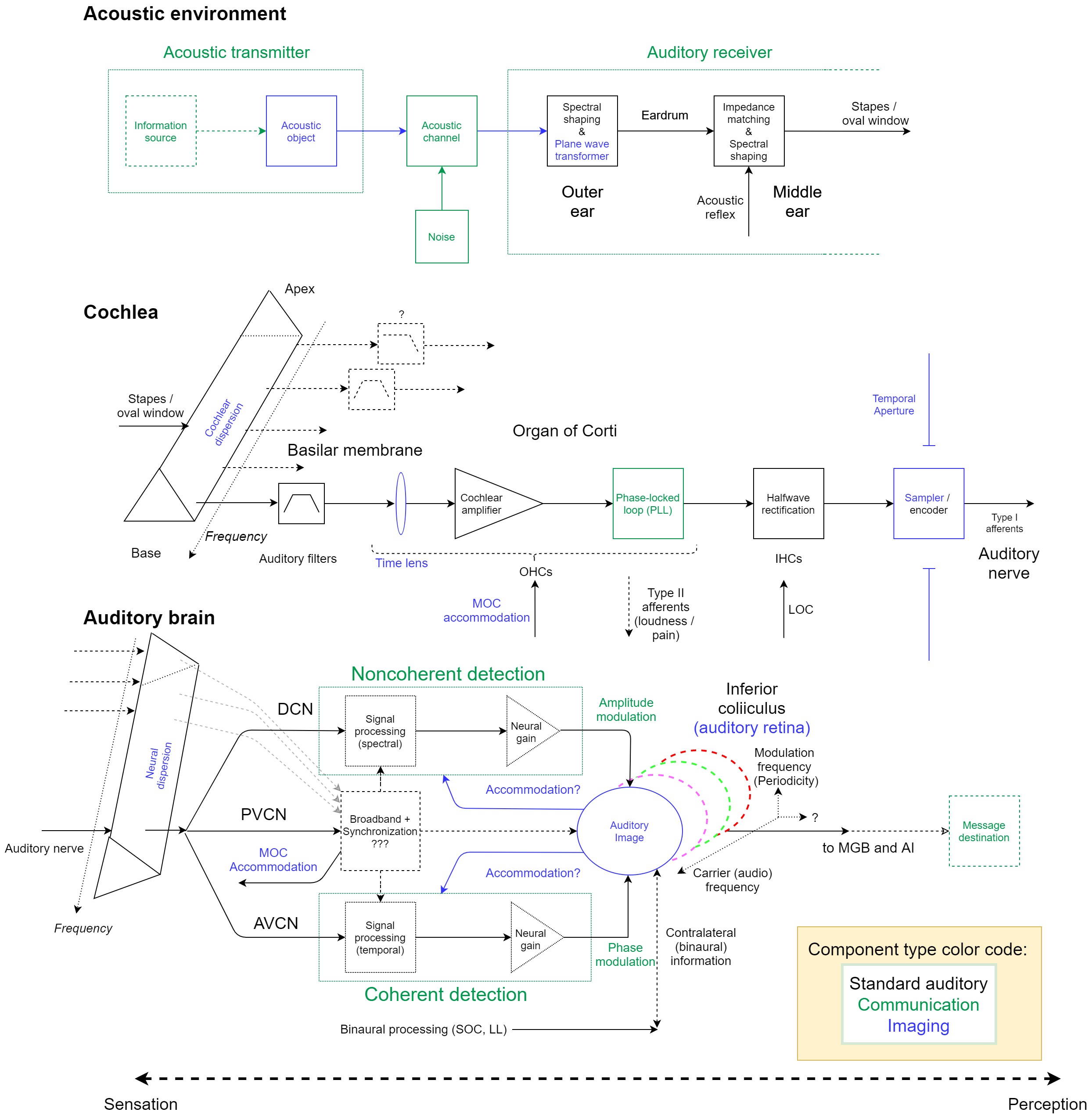
Chapter 2 The anatomy and physiology of the mammalian ear
2.1 Introduction
The ear structure is similar across all mammals and interspecies differences appear to be primarily morphological, relating to the size, shape, and layout of the different parts. The mammalian auditory periphery is subdivided into outer (or external) ear, middle ear, and inner (or internal) ear, which includes both the cochlea and the auditory nerve. Subsequently, the auditory nerve projects to the central nervous system, which comprises a number of auditory nuclei in the brainstem, midbrain, thalamus, and cortex.
Much of the experimental and theoretical work in physiological hearing research has revolved around the cochlea, where the most significant signal transformations take place. Whatever kind of transformation or processing occurs in the cochlea, its effects can usually be measured downstream, in the auditory brain. However, since the cochlea is remarkably complex, concealed, and vulnerable, its exact function and micromechanics are not well understood. Other elements of the central part of the auditory system are even less well understood.
As the anatomy and physiology of the ear has been covered in numerous texts in great detail, it will not be covered here in depth. Instead, the emphasis in the following is on coarse-grained components and functions of the human auditory system that are relatively uncontroversial, up-to-date, and informative for a high-level analysis. Therefore, the typical description of the micromechanics of the cochlea or the cell types in the brain with their specific responses is usually avoided. Unless referenced otherwise, the review in § 2.2 and § 2.4 is largely based on Pickles (2012). Additional presentations of the human ear’s structure are found also in Fuchs (2010) and Rees and Palmer (2010) and shorter introductions in Møller (2012) and Gelfand (2018).
When discussing the neurophysiology of the auditory brain, the lack of a coherent theory for it, and for hearing in general, becomes a stumbling block for the understanding of what this complex system does. Therefore, before reviewing the central auditory system, a discussion is provided in § 2.3 that provides a few general guiding principles and theoretical ideas that have been commonly employed in auditory neuroscience research, as well as some of their critical shortcomings. The few theories about specific auditory nuclei are then briefly mentioned, where available, throughout the review in § 2.4.
Since much of the knowledge about the human ear’s anatomy has been gathered from animal data, it is essential to know how the auditory systems of these animal species differ. The final section (§ 2.5) deals specifically with the comparative anatomy between mammals. It too is a selective and coarse-grained review of some of the notable differences between animals, given the commonalities covered in § 2.2 and § 2.4. Therefore, it is somewhat unlike typical comparative hearing texts that tend to focus on specific organs within a subset of animals and to review their similarities as well. This part of the review is based primarily on Rosowski (1994) for the outer and middle ears, Echteler et al. (1994) for the cochlea, and Glendenning and Masterton (1998) for the central pathways. In-depth reviews of various topics in comparative hearing of mammals (and other vertebrates) can be found in volumes edited by Popper and Fay (1980); Popper and Fay (1994); Manley et al. (2000) and Köppl et al. (2014).
2.2 The peripheral ear
Many parts of the peripheral ear have at least two anatomical terms that are in regular use. Where available, we present both terms with the lesser used term in the present text given in parentheses.
2.2.1 The outer ear
Acoustic waves in the environment propagate from their source through a medium—either air or water—before entering the external ear, whereupon they begin a sequence of transformations. Sound is diffracted by the pinna (or auricle)—the cartilaginous external part of the ear, which is connected to the concha that is shaped like an irregular horn. The pinna and concha collect the impinging sound to efficiently radiate it into the ear.
The sound then passes through a hard-walled ear canal (or auditory meatus) that terminates with the eardrum (tympanic membrane), which is a thin membrane that vibrates with the sound pressure. The ear canal has a few resonances that emphasize certain frequencies (most prominently at around 2.5–4 kHz for humans), which are determined mainly by its length (Wiener and Ross, 1946; Shaw, 1974; Mehrgardt and Mellert, 1977). The sound field that reaches the eardrum is one-dimensional, in very good approximation, especially at low and midrange frequencies, since the ear-canal diameter is much smaller than the wavelength at this range (Rabbitt and Holmes, 1988). The pinna spectrally shapes the sound as well, but in a direction-dependent manner that has a role in localizing the elevation angle of the sound source. This feature, along with its efficient sound power delivery, are thought to be the two main acoustic functions of the outer ear (Rosowski, 1994).
2.2.2 The middle ear
On the internal side of the eardrum, the vibrations in the air or water medium push a mechanical system made of three small bones, the ossicles—the malleus (hammer), the incus (anvil), and the stapes (stirrup)—which constitute together the ossicular chain of the middle ear. The ossicles are positioned within an air cavity, whose pressure is regulated through the eustachian tube, which is connected to the pharynx at the back of the mouth. This anatomy was already described in great detail by 543 pp. 129–135 along with a hypothetical model of operation that has been partially confirmed since. The malleus is attached to the stretched eardrum in the umbo at its center, whereas the stapes is attached via the annular ligament to another membrane—the oval window, which is part of the cochlear wall. The eardrum, umbo, and ossicles are coupled rigidly at low frequencies, but higher modes of vibration (e.g., bending of the ossicles) and other degrees of freedom in their movement (compression of the ossicular joint or the ligaments between the ossicles, or multimodal motion of the ear drum) may diminish the effectiveness of the coupling at higher frequencies.
The outer and middle ears work together as a non-ideal (frequency-dependent) transformer between the acoustic impedance (the ratio between the pressure and volume velocity) of the air and that of the incompressible fluid of the cochlea. The middle ear also functions as a mechanical lever, which transforms the power exerted on the eardrum to much larger power on the oval window, which is of a smaller area than the eardrum. In humans, the gain it provides has a bandpass filter characteristic with a maximum at 1200 Hz and approximately -6 and -7 dB per octave below and above, respectively (Aibara et al., 2001). However, the impedance is not necessarily resistive and complex relations between the pressure and velocity may exist. The vibration of the middle ear is linear with input level below 96 dB SPL and has negligible nonlinear distortion up to 130 dB SPL—well above the ecological sound range (Guinan and Peake, 1967; Aerts and Dirckx, 2010). Its output is the movement of the stapes that is coupled to the cochlea, which moves one-dimensionally like a piston below 6.7 kHz, but has more complex rocking motion at higher frequencies (Aibara et al., 2001).
Two muscles are connected to the ossicles that control the acoustic reflex—the tensor tympani is connected to the malleus and the stapedius is connected to the stapes. Both appear to regulate the transmission gain of the middle ear, particularly below 1 kHz, by stiffening the ossicular movement, which causes an increase of acoustic impedance. The result may provide some protection against loud sounds and act as automatic gain control. It is also thought to reduce self-generated sounds by the listeners and to selectively reduce low frequency sounds that can cause undesirable masking. However the function of these reflexes is not well understood.
The middle ear is a critical stage in hearing that provides necessary amplification in hearing. An impaired middle ear can lead to a conductive hearing loss.
2.2.3 The inner ear
2.2.3.1 The cochlea
The cochlea is a spirally shaped structure that is located inside the anterior portion of the petrous region of the temporal bone, along with the semicircular canals of the vestibular system that occupy its posterior region (Echteler et al., 1994). The coiled tube is longitudinally divided into three fluid-filled compartments, whose cross section is illustrated in Figure 2.1. The first compartment, the scala vestibuli, is where the oval window is located. The motion of the stapes presses the elastic oval window and thus the cochlear fluid, the perilymph, which is largely incompressible (with approximate fluid properties of water and composition similar to extracellular fluid). Scala vestibuli terminates in an opening called the helicotrema, where the compartment connects to scala tympani, which is another compartment that leads back through the entire length of the cochlea. The oval window displacement causes a corresponding displacement of the round window, at the other end of scala tympani.
The two scalae are separated by elastic membranes, which tightly enclose on the scala media (or cochlear duct)—another compartment that is not directly connected to the other two and is filled with endolymph, or endocochlear fluid (see Figure 2.2). The endolymph is similar in properties to intracellular fluid that is rich with potassium and low in sodium ions that make the scala positively charged in reference to the perilymph by about about 80–100 mV. The supply of ions originates in the stria vascularis, on the wall of scala media, which has a capillary supply. The membrane below scala vestibuli is called Reissner’s membrane and it does not have a direct role in the sound transduction chain, although it has been proposed that it takes part in the reverse transmission the otoacoustic response from the ear (Reichenbach et al., 2012). The fibrous membrane above scala tympani is called the basilar membrane (BM) and it is attached to the organ of Corti—a complex structure of cells that transduces the mechanical movement to electric discharges in the auditory nerve. The elastic BM moves in response to a pressure gradient between the scala vestibuli and scala tympani. This movement manifests as a slow traveling wave that propagates from the oval window in the base of the cochlea toward the helicotrema in its apex.

The cochlea has unique frequency analysis properties, whose mechanics was largely elucidated by Békésy (1960). High frequencies conducted through the stapes vibrations cause the BM to vibrate at the base, while low frequencies vibrate at the apex, in terms of the traveling wave peak response. For a given stimulus frequency, the wavelength and phase of the traveling wave change quickly and slows down just before the frequency-dependent peak, whereupon it dies out almost immediately after the peak with little to no energy reflected back to the base. The peak sharpness is reduced at high intensities. The frequency analysis property is achieved by the particular geometry and mechanics of the cochlea, which is tapered in two opposite directions: the ducts are wide at the base and narrow at the apex, whereas the BM is wide at the apex (about 0.5 mm) and narrow at the base (0.1 mm). Critically, the forward direction of the movement is largely determined by the stiffness of the BM that is high at the base and gradually diminishes towards the apex, where the BM movement is mass-controlled.
The organ of Corti is attached to the BM by supporting cells that embed the inner hair cells (IHCs) and outer hair cells (OHCs). Both hair-cell types comprise of a soma (cell body) and a hair bundle, or stereocilia. These stiff hair-like structures protrude from the apex of the cell, which is flushed with the reticular lamina—a thin membrane inside the organ of Corti, which chemically isolates the perilymph from the endolymph. The IHCs are organized in a single row and the OHCs in three or more rows along the cochlea. The hair bundle is graduated in height and it forms straight (IHCs) or V-shaped (OHCs) patterns that are apparent on the reticular lamina. The stereocilia within one hair cell are connected to one another via small horizontal top connectors and tip links, so that the entire hair bundle rigidly deflects upon mechanical force and it bends around its base. The side links of the OHCs provide mechanical reinforcement against loud sounds (Han et al., 2020).

The traveling wave in the BM causes a shearing movement of the organ of Corti, which leads to deflection of the stereocilia of the hair cells. In turn, this deflection of the IHCs causes the tiny tip links between the hairs to open and close mechanotransducer channels in the apical end of the stereocilia, close to the tip links. This leads to ionic current flow from the positively-charged endolymph to the negatively-charged cell and then to neurotransmitter release (likely, glutamate, although not exclusively; Eybalin, 1993) to the synapse of the auditory nerve. The opening of the channel is asymmetrical with respect to the direction of deflection of the hairs, which results in a mixed AC and DC response potential. The hair cell response reflects the mechanical response of the BM around its peak, whose corresponding frequency is referred to as the characteristic frequency (CF).
The tectorial membrane (TM) is an elastic gelatinous membrane that is flapped over the hair bundle rows and the reticular lamina. Unlike the BM, the TM is found in all tetrapods, but its role in the cochlear micromechanics remains uncertain. The tallest OHC sterocilia are connected to one another and to the TM by TM-attachment crown, which are essential for the normal OHC function (Han et al., 2020). It has been found very recently in guinea pigs that both the IHCs and OHCs are deeply embedded inside the TM (Hakizimana and Fridberger, 2021). It was also found that all hair cells are connected to the TM with filamentous tubes called Ca2+ ducts, which directly supply calcium ions to the hair cells that are required for the OHC motility. In the same study it was shown that the TM rests on the RL with no gap between them in quiet, and that their movement remains tight also at large amplitudes, only with momentary gaps when the system returns to quiet. During stimulation, the OHCs and the IHCs appear to be phase locked. These results contradict past findings that were done using coarser methods that only found that the only Ca2+ supply to the bundle is from the endolymph, that the tallest OHC tips are embedded in the TM, and that the IHCs are not directly connected to it, although their tips fit into a groove on the bottom of the TM (Hensen’s stripe).
It was demonstrated in human cadavers and in mice that the TM sustains a traveling wave as well, which in comparison with the BM has sharper tuning, apically shifted frequency mapping, and larger dynamic range (Lee et al., 2015; Farrahi et al., 2016). Shearing motion of the RL translates to TM motion that can move the IHC hair bundle through fluid forces (Zwislocki, 1980; Cheatham and Dallos, 1999; Robles and Ruggero, 2001). Other recent findings in mice suggest that the role of the TM may be in stabilizing the cochlear mechanical amplification (see below), as detached TMs result in high incidence of spontaneous otoacoustic emissions (Cheatham et al., 2016).
The passive system in the cochlea cannot achieve on its own the tuning sharpness of the BM that is observed empirically, so there is little doubt today that the OHCs provide the compressive amplification necessary for the healthy cochlea to hear sounds at adequate level (Robles and Ruggero, 2001). The OHCs possess two candidate mechanisms that can drive this amplification (Kennedy et al., 2006). Both mechanisms are induced by the shear forces on the organ of Corti, which moves with the vibrations of the traveling wave in the BM. The cochlear motion causes deflection of the stereocilia, which gates mechanotransducer ion channels that set the current flow into the cells. The most prominent active mechanism is the somatic motility, or electromotility, of the hair cells. It involves length changes of the hairs when intracellular electric current passes through the cells and causes somatic lengthening with hyperpolarization and shortening with depolarization (Brownell et al., 1985). In vitro, this movement can take place at ultrasonic frequencies (shown at least up to 79 kHz, Frank et al., 1999). The exact dynamics of this mechanism—how it actually delivers power that impacts the signal picked up by the IHCs—is not entirely clear. One influential class of amplification models requires that the motile changes happen in phase with the traveling wave, on a cycle-by-cycle basis (Dallos et al., 2008; Guinan Jr, 2020). However, this view is challenged because electromotility may be limited to much lower frequencies by the capacitive cell membrane in-vivo and more realistic in-vitro conditions (Dallos and Evans, 1995; Ashmore, 2008; Vavakou et al., 2019; Santos-Sacchi, 2019; Santos-Sacchi and Tan, 2019). Electromotility is associated with the protein prestin (Zheng et al., 2000), and in mutated mice that lack prestin, there is no amplification or compression (Liberman et al., 2002). Counterexamples exist for the presence of prestin with no amplification in birds (e.g., in chickens, Xia et al., 2016), and electromotility on its own does not guarantee amplification also in mammals (gerbil in Strimbu et al., 2020). Alternative models to amplification work by locally modifying the impedance of the basilar membrane, thereby creating a sharper resonance with less dampening (Kolston, 2000; Vavakou et al., 2019, e.g.,). These length changes, as well as other biophysical changes in the cell, can result in substantial OHC stiffness modulation (Ashmore, 2008). The other active mechanism of the OHC is the motion of the hair bundle (the stereocilia), or bundle motility, that protrudes from the apex of every hair cell, at the reticular lamina, and is most likely mechanically connected to the TM. It seems that whichever mechanism is responsible for the cochlear amplification, it requires a certain feedback between the BM, the OHC soma, the hair bundle, and perhaps other elements such as the TM (see § 9.8.2 for feedback model references). It was also hypothesized that the two motile effects may be both necessary to achieve the OHC amplification in mammals (Peng and Ricci, 2011).
The OHCs are implicated in a host of nonlinear phenomena in the cochlea. First and foremost, they provide amplification around the characteristic frequency for low-level inputs, which results in effective lowering of the hearing threshold. Consequently, it also sharpens and shapes the filter response around the CF. Most models that account for amplification require some kind of feedback between the energy that is delivered back to the BM from the organ of Corti. Additionally, the OHCs cause compression of the dynamic range of the input at medium levels (approximately 30–90 dB SPL), they are implicated in intermodulation distortion generation, in two-tone suppression, and in otoacoustic emissions. The OHCs require metabolic supply of energy, which means that their associated functions cease to work after death. Recent evidence has suggested that, the amplification and the other active effects take place inside the organ of Corti, so they are measurable on the reticular lamina, but not necessarily in the BM (Ren et al., 2016a; Cooper et al., 2018; Nuttall et al., 2018; He and Ren, 2021, e.g.,).
2.2.3.2 The auditory nerve
The vestibulocochlear nerve, which is the eighth cranial nerve, is shared between the vestibular and auditory (cochlear) nerves (Rea, 2014, pp. 81–93). The human cochlea is innervated by approximately 30000 afferents of the spiral ganglion neuron type and about 1400 efferents, which form the auditory nerve. Most fibers are Type I, which are fast (both fibers and soma are myelinated) bipolar cells, whose dendrites synapse to IHCs and axons synapse to the auditory brainstem nuclei. Each IHC is connected to 10–30 Type I fibers with a single ribbon synapse per fiber, which are characterized by their reliable, temporally precise, and sustained responses. Type II fibers are slow (unmyelinated) unipolar cells that innervate up to 50 OHCs each. The OHCs are synapsed to multiple Type II fibers. Both types project to the cochlear nucleus in the brainstem, which is the first nucleus in the central auditory pathway.
It is common to refer to the discharge patterns in the auditory nerve as the earliest part of an auditory neural code. It has been extensively studied in single-unit recordings in many species, mostly for relatively simple signals (Eggermont, 2001; Rutherford et al., 2021, e.g.,). The code varies in its rate and inter-spike patterns, with respect to the input stimulus level, temporal, and spectral characteristics. Fibers (Type I) are characterized by their spontaneous discharge rate, which reflects their inherent noise level and may be low, medium, or high. High-spontaneous-rate fibers are most sensitive to low-level inputs and are the most prevalent (90% of all fibers), but have a relatively limited dynamic range of about 20–30 dB. The low-spontaneous-rate fibers are sensitive to high levels and have wider dynamic range of up to 60 dB. The frequency tuning of the fibers reflects the bandpass characteristics of the cochlea, which is often illustrated using tuning curves of the effective filtered response. At the CF, the spiking rate is maximal (for a given input level). Another important feature of the auditory nerve spiking is phase locking—a precise temporal correspondence between the (tonal) stimulus wave phase and the neural spiking pattern in the auditory nerve and most other nuclei. Phase locking is limited to low frequencies (estimated to be below 4 kHz for humans). The auditory nerve can also track the low-frequency stimulus envelope for all carrier frequencies (also above 4 kHz). The function of Type II fibers has been recently elucidated in experiments on mice in vivo, where a non-acoustic nociceptive (pain) reaction to very loud sounds (120 dB SPL) has been established, which leads to avoidance behavior (Flores et al., 2015). In-vitro tests found that these fibers react to OHC damage, as the kind that occurs with the traumatic exposure to loud sounds and is irreparable in mammals (Liu et al., 2015).
Descending efferent innervation to the hair cells exists in the cochlea as well, which is called the olivocochlear bundle. It arises in the superior olivary complex (SOC) of the brainstem and has two divisions. The medial olivocochlear (MOC) efferents, are myelinated and they project both to the contralateral and ipsilateral OHCs with cholinergic synaptic contacts to the cell body. The lateral olivocochlear (LOC) fibers are unmyelinated and they project mainly to the ipsilateral afferent dendrites of the IHCs, but not directly to the hair cell body. The MOC receives afferent input from the auditory nerve via the poteroventral cochlear nucleus (PVCN), which projects to the contralateral SOC. Activation of the MOC causes a bilateral change of threshold through the the medial olivocochlear reflex, which has two pathways—an ipsilateral reflex and a contralateral reflex. Fibers that respond to monaural sounds are the majority and both ipsilateral and contralateral synapse to the OHCs in the same way, although there are about double the number of ipsilateral as there are contralateral fibers, as well as a much smaller number of binaural fibers that respond to stimulation from both ears (Liberman and Brown, 1986; Brown, 1989). Accordingly, the ipsilateral reflex effect (gain magnitude) has been consistently stronger than the contralateral effect in humans (Salloom and Strickland, 2021). The MOC efferents are tuned to the same frequencies as the OHCs they innervate, although their activation is proportional to the bandwidth of the stimulus, where broadband noise is typically used. While uncertain, it has been proposed that the olivocochlear bundle may provide some protection against acoustic trauma including own voice attenuation, regulate the operating point of the amplification, optimize detection of signal in noise (i.e., reduce masked tone threshold), and reduce the sensitivity to unattended stimuli (see also § 16.4.2).
2.3 Organizing principles and common threads in the
central auditory system
Unlike many parts of the peripheral ear, the functions of the different auditory nuclei have so far eluded a plain explanation. The auditory neuroanatomy has been thoroughly charted, but the complexity of the parts forming the system as a whole are prohibitive in the formation of a simple functional account. In order to facilitate the description of the system, several general and particular aspects of the auditory brain are discussed in brief. Some of these principles are not unique to hearing.
The central auditory system comprises several nuclei and multiple pathways for the signal to travel downstream to the cortex (the major pathways are illustrated in Figure 2.3). Each nucleus has several neuron types, which can be characterized by different morphologies and typical responses to different stimuli, usually using single-unit (e.g, one neuron) measurements. The auditory nuclei further project to other auditory and occasionally non-auditory nuclei, which may be either excitatory or inhibitory. The connections and responses of the different neuron types have been studied in depth over the last decades, and functions of the respective areas were sometimes inferred from these responses. However, the complexity and diversity of the complete system makes it very challenging to attribute a “closed-form” function to most, if not all, of the auditory nuclei.
2.3.1 Tonotopy
Perhaps the most characteristic organizing feature of the auditory system is that the cochlear frequency axis, its tonotopy, is conserved throughout the auditory brain. Thus, the same monotonic arrangement of frequencies from high to low is found in all of the main auditory nuclei. For example, in the cat, tonotopy was recorded in the cochlear nucleus, lateral lemniscus, inferior colliculus (IC), medial geniculate body (MGB), and auditory cortex (Bourk et al., 1981; Aitkin et al., 1970; Merzenich and Reid, 1974; Aitkin and Webster, 1972; Reale and Imig, 1980). Importantly, even though the early brainstem nuclei have their own tonotopic maps, they all converge to a single map in the inferior colliculus (Casseday and Covey, 1996). Additionally, in the human primary auditory cortex, tonotopy may be different from the more peripheral nuclei, as it maps to pitch rather than to frequency, as can be measured in the magnetoencephalogram (MEG) response to the missing fundamental (Pantev et al., 1989). However, this finding was inconsistent with single-unit recordings in cortices of other animals and appears to be confined to relatively small cortical areas (see references in Gander et al., 2019, Section 4.5).
Starting from the IC and extending to the MGB and auditory cortex, a useful classification of the different auditory stations is into lemniscal pathways that are more sharply tuned and are organized tonotopically. They are the primary ascending conduit of auditory sound information from the periphery (Carbajal and Malmierca, 2018). In contrast, non-lemniscal pathways constitute the “belt” areas that are less responsive to auditory stimuli, are not organized tonotopically, send ascending pathways to the next nucleus, and receive descending connections from the cortex. However, it has been recently suggested that the non-lemniscal corticocortical circuits may be involved in complex processing of speech that is parallel to that of the core and its associated lemniscal pathway (Hamilton et al., 2021). We will mostly consider the lemniscal nuclei in the review below.
2.3.2 Synchronized responses
Another important property that is used to characterize different neuron types is their degree of phase locking, or synchronization—how well they track the acoustic waveform of the stimulus (see § 9.7.2). Some nuciei and particular cell types seem to excel in synchronizing either to the carrier or to the envelope. The degree of synchronization to the stimulus can be enhanced through an increase in the number of dendrites that synapse the synchronizing cell. This is the case since multipolar cells generally have high threshold for firing, which means that several input fibers have to fire simultaneously in order for the cell to fire. When all the inputs are excitatory, such a configuration is sometimes referred to as a coincidence detector—a useful circuit in the enhancement of the temporal response of the neuron (see § 8.5). Another aspect in which cells vary is whether they synchronize to stimulus onsets or to sustained stimuli, as some cells synchronize to one feature and not to the other. Either way, the response usually shows spiking adaptation over time—a reduction in the average spiking rate—in response to an unvarying stimulus.
2.3.3 Generalizations from single unit recordings
Because of the complexity of the auditory system, as well as neural systems in general, it is difficult to attribute specific functions for the brainstem circuitry. Hence, the understanding of the roles of many auditory nuclei remains relatively vague. Pickles (2012, pp. 155–157) categorizes the central auditory system research findings into overarching themes, all of which are also encountered in non-auditory sensory research1919 19 Pickles (2012) presented three themes, but we merged the first two into a single theme, as they are difficult to distinguish in the original text.:
- 1.
Feature detection and extraction—Relevant auditory features from the stimulus (e.g, spectrum, temporal fluctuations, sound location) may be observable through recordings of a single unit. It may also be associated with a population of neurons that is localized in a certain brain area and has a modular role in the complete signal processing chain.
- 2.
Hierarchical analysis—It is sometimes possible to demonstrate progression in complex auditory processing that emerges in one auditory area and culminates in another, usually more central in the ascending pathways (e.g., the auditory cortex as the destination area of auditory scene analysis). This theme introduces continuity and causality into the information-processing logic of different auditory areas in the brain.
These themes are interdependent and find wide use in auditory research. However, they require external theories to direct the experimental explorations and inspire plausible interpretations. A lack of theory makes the interpretation much more challenging due to the complexity of the system. This was illustrated in a critical paper called “Could a neuroscientist understand a microprocessor?’’2020 20 It was inspired by an earlier paper called “Can a biologist fix a radio?—Or, what I learned while studying apoptosis” (Lazebnik, 2002), which may have some relevance to complex structures in the peripheral ear, such as the organ of Corti. (Jonas and Kording, 2017). The premise of the paper is that reverse engineering of even a relatively simple computational circuit may be downright impossible using many of the standard methods in neuroscience. Their example was a (simulation of a) popular microprocessor from 1975 that contains 3510 transistors in total, which in today’s standards would be considered primitive. It was made to run a number of simple video games as known “behaviors”. Transistors in the circuit were taken as rough analogs of neurons. Employing classical neuroscientific methods produced a wealth of data and many distinct patterns, which were nevertheless useless in explaining what the microprocessor actually does on a level that can be generalized beyond the specific game being played.
While these conclusions from Jonas and Kording (2017) may appear dispiriting (and perhaps controversial), they are invoked to highlight the nontrivial implications of a lack of a coherent theory of the auditory brain pathways. Local simplicity of brain functions, including low-level ones as observed using simple stimuli in single unit recordings, might be misleading, especially if tested with a narrow range of stimuli. As illustration, a recent comparison of several phenomenological and biologically-inspired auditory signal processing models demonstrated that the simplest model has the highest correspondence to single-unit recordings from the ferret primary auditory cortex, using several simple stimuli (clicks, pure tones, white noise, speech snippets; Rahman et al., 2020). The authors suggested that this surprising result can entail that the total effect of the auditory system is much simpler than its complexity may imply. However, their interpretation entails (with some exaggeration, admittedly) that for the tested stimuli the brainstem processing may as well be replaced with direct connections to the cortex, as long as the necessary frequency weighting and nonlinear compression is reproduced. While not unique to this model or study, such oversimplification leads to tagging entire networks with the infamous “relay neuron” role (often designated to the thalamus). To this Winer and Schreiner (2005b, p. 46) commented: “The concept of a relay nucleus requires critical scrutiny as all central nuclei transform and modify the information that passes through them…” Another problem with this interpretation is that it implies that the single-unit primary auditory cortical response is tantamount to a perceptual and behavioral output. It was recently argued that spiking patterns cannot be simply replaced in analysis with more informative signals or inputs, as these patterns do not generalize to real-world stimuli with arbitrary context (Brette, 2019).
Another point of view to consider continues the microprocessor analogy, where the auditory brain is thought to perform some computational task. Hypothetically, any computation requires not only the transmission of the data, but also the transmission of various control signals to modulate its processing, according to the situation. The auditory system processes signals that are on the same temporal scale as the neural processing speed limit. Thus, neuron spiking patterns may correlate to acoustic signals with relatively few transformations throughout the brain, which reduce its complexity and maintains clear correspondence between stimulus and response. However, internal control signals that may be internally used for computational purposes may be correlated with the stimulus as well. This may result in a cacophony of control and sensory signals in the brain that are correlated on a population level, but have fundamentally different roles in the system as a whole.
In summary, getting a handle on the brain function requires a theory for guidance, which is especially pertinent in the auditory system due to its high complexity. Developing a theory from the reduced low-level components may be hypothetically possible, but it will require a way about compressing the amount of low-level details to a compact description, which can be formulated using high-level concepts. There is no guarantee that this is the case, though. Quoting Winer and Schreiner (2005b, p. 45) again: “It may not be possible or even appropriate to delegate functions to nuclei, as functions are global constructs, while neurons and nuclei and circuits are restricted to local operations.”
2.3.4 Dual-stream models
We shall mention one organizational theory that has been influential in recent hearing research that may apply to the entire auditory system—the dual stream model. It was originally proposed for vision by Trevarthen (1968) and Schneider (1969) and has been revised several times since. According to this model, the processing of visual objects bifurcates in the cortex. The ventral stream, or the what stream, processes the pattern (shape) and the identity of the object, whereas the dorsal stream, or the where stream, processes its position in space (Mishkin et al., 1983; Wilson et al., 1993). Analogous functions were identified in two distinct anatomical streams going out of the auditory cortex that pertain to identification and localization (Rauschecker, 1998; Kaas and Hackett, 1999; Romanski et al., 1999).
The neat labor-division offered by the dual-stream model turned out to be more complex both in vision and in hearing. In vision, object localization processing is tied to motor control functions that may be required for actions based on the visual input (Goodale and Milner, 1992). Thus, a revised dual-stream model in vision distinguishes vision-for-perception (ventral) and vision-for-action (dorsal) streams (Goodale, 2011). A more recent version of the model identifies a third visual processing stream that specializes in motion or socially relevant objects (e.g., faces, body movements) (Pitcher and Ungerleider, 2020). A similar refinement has been applied in hearing, as it became clear that the dorsal stream does not process localization exclusively, but also has some roles in speech and even music processing that require tracking acoustic changes over time (Belin and Zatorre, 2000; Hickok and Poeppel, 2004; Hickok and Poeppel, 2007). The ventral stream in speech may be suitable for recognition of words, which are sometimes classified as auditory objects. Thus, a unified model is emerging that posits that language may require processing that relies on both streams, which include sensorimotor connections with articulators that may be used to produce speech (Rauschecker, 2017; Rauschecker, 2018). This interpretation would be a special feature of the human cortex, with unknown applicability to other mammals.
The dual-stream model has also influenced the interpretation of subcortical processing that is known to bifurcate early in processing (in the cochlear nucleus) into several parallel streams that converge again only in the midbrain (inferior colliculus; Pickles, 2012, Chapter 6). The early ventral stream does seem to be dedicated mostly to binaural localization, but the roles of the other two streams are not obvious. Another version of the dual-stream model for speech suggested that the brainstem may be separately processing the fundamental frequency of speech and spectral changes in time—at least as early as the lateral lemniscus and inferior colliculus (Kraus and Nicol, 2005). However, as has turned out in the cortical stream modeling, the subcortical streams do not readily lend themselves to neat classification as the original what/where model suggested, or to other obvious signal processing, so their explicit functions are not necessarily clarified by this model.
2.4 Central auditory neuroanatomy
This section provides a simplified overview of the complex circuitry in the auditory brainstem. Only high-level details that may have greater functional significance for the system are mentioned, while most of the fine-grained details are omitted.

2.4.1 Medulla and pons
Auditory nerve fibers innervate the cochlear nucleus, where they branch to three cochlear nucleus (CN) areas. The axons from these nuclei run in three different tracts, or acoustic strias, which lead to further nuclei (Cant and Benson, 2003). The rostral branch begins from the anteroventral cochlear nucleus (AVCN), which is one of the two divisions of the ventral cochlear nucleus (VCN)—the other being the posteroventral cochlear nucleus (PVCN). The AVCN receives its input from the endbulbs of Held — giant synaptic terminals with multiple synapses. The endbulbs of Held are characterized by reliable spiking in response to auditory nerve spikes, as well as very short delays as the synapses are positioned on the soma itself. The AVCN appears to have little or no inhibitory inputs, so its response largely reflects that of the auditory nerve.
The AVCN projects contralaterally to the medial superior olivary (MSO) and ipsilaterally to the lateral superior olivary (LSO)—both are nuclei of the superior olivary complex (SOC). The LSO also receives inhibitory input from the contralateral VCN via the medial nucleus of the trapezoid body (MNTB), which contains the largest synaptic terminals in the brain—the calyx of Held—that enable temporally precise spiking. The SOC is critical in binaural functions, where the LSO primarily extracts interaural loudness difference (ILD) cues at high frequencies, while the medial superior olive (MSO) primarily extracts interaural time difference (ITD) cues at low frequencies. The MSO has additional capabilities in extracting fine temporal cues that are monaural (e.g., echo suppression), at least in small mammals that do not exploit interaural localization cues, such as bats and rats (Grothe, 2000). The SOC is also where the olivocochlear bundle arises, which projects contralaterally to the OHCs (the MOC), ipsilaterally to the IHCs (the LOC), as well as collaterally to the CN.
The caudal branch of the CN innervates the PVCN and the dorsal cochlear nucleus (DCN). The PVCN contains four different cell types with unique responses. Among them are onset detection by octopus cells of broadband sound (e.g., clicks), which are temporally precise. Another interesting cell type is the chopper (T-stellate) multipolar neuron, which is sharply tuned in frequency and fires with a sustained period that is independent of the input frequency but closely tracks its envelope. The T-stellate cells project to the MOC cells in the SOC, among others. The PVCN cells project ipsilaterally and contralaterally to most neighboring nuclei, including the VCN, the ventral nucleus of the lateral lemniscus (VNLL), and the inferior colliculus (IC). Additionally, they project to the superior paraolivary nucleus (SPN), which is a part of the SOC, but has a monaural function in precise offset and (much less in) onset detection in complex sounds (Felix II et al., 2017; Kopp-Scheinpflug et al., 2018). Therefore the PVCN plays a role in all auditory functions, yet a single specific role cannot be easily pinned down.
The DCN is composed of a complex network of cells with diverse responses and numerous connections to other nuclei. In addition to auditory inputs, it receives and projects to somatosensory cells around the pinna. This is thought to reflexively affect localization optimization in animals that can move their external ears, which can have a role in detecting elevation localization cues. It may also have a role in suppression of the input of own vocalizations. Like other areas in the CN, the DCN receives excitatory and inhibitory inputs from most other auditory nuclei, which can change the tuning curve bandwidth of the different cells, or modify their dynamic range by shifting the threshold for firing. Its main projections are to the inferior colliculi on both sides. The DCN is also implicated in sound offset detection and as such it may constitute a part of a specialized “offset pathway” along with the SPN, the IC and the medial geniculate body, which appears to be distinct from an “onset pathway” in the auditory brain (Kopp-Scheinpflug et al., 2018).
The CN receives centrifugal (descending) efferent innervation from the IC and from the auditory cortex, which is implicated in modulation of the critical bandwidth of the auditory filters and changing of the masked threshold for tone in noise. The centrifugal inputs may also affect the time constants associated with masking, as well as spike timing modulation by somatosensory inputs to DCN neurons.
The next stage after the CN and SOC is the lateral lemniscus tract, which has three nuclei—the ventral, intermediate, and dorsal nuclei of the lateral lemniscus (VNLL, INLL, and DNLL, respectively). The DNLL is part of the localization stream as it receives inputs from the LSO, MSO and CN and projects to the IC on both sides. It has been suggested that the DNLL is key in inhibiting the reflection (the lag) in the (binaural) precedence effect, which then gives precedence to the direct (the lead) sound at the level of the IC (Brown et al., 2015).
The VNLL receives projections from the ipsilateral MNTB and the contralateral VCN, but is completely bypassed by projections from the DCN and SOC. The VNLL projects mainly to the ipsilateral central nucleus of the IC (ICC). As it receives its input mainly from the octopus cells, it exhibits temporally precise but complex responses, which do not disclose an obvious function. An unusual feature of the VNLL is that its tonotopic axis is folded in a three-dimensional helicoidal topology, so that its peripheral laminae are mapped to low frequencies of the IC and the central laminae are mapped to high frequencies (Merchán and Berbel, 1996). This structure was compared with the musical pitch helix and associated with auditory sensitivity to periodicity, and hence, was implicated with the basis for harmonicity detection (Langner, 2015; but see Regev et al., 2019).
The function of the INLL is even less clear than the VNLL and DNLL. The INLL primarily projects to the ipsilateral IC and receives its major projections from the ipsilateral MNTB (inhibitory) and the contralateral AVCN and PVCN (excitatory), but with lighter projections from other ipsilateral CN and SOC nuclei (Kelly et al., 2009; Yavuzoglu et al., 2010). It was shown in bats that high-frequency INLL units can be inhibited by low-frequency non-tonotopic sounds—spectral shaping that most likely carries over to the IC and maybe to the auditory cortex (Yavuzoglu et al., 2010).
There is no generally accepted theory for the function of the lower brainstem nuclei, except perhaps for the localization done by the SOC (Glendenning and Masterton, 1998, e.g.,). The early bifurcation in the auditory pathways at the CN suggests that its different subnuclei have different functions in processing the stimulus. Studies in the avian analogs of the CN, which are simpler than the mammalian CN2121 21 The avian auditory brainstem pathway splits to two well-separated streams, instead of three. In the barn owl, this separation is retained also in the processing of interaural time and level differences until they converge at the inferior colliculus (Takahashi et al., 1984)., suggest a simpler role division in the barn owl (Sullivan and Konishi, 1984) and chicken (Warchol and Dallos, 1990). The cochlear magnocellularis (the avian homolog to the AVCN) is particularly sensitive to temporal changes, judging by its enhanced phase locking to stimuli. At the same time, it is relatively insensitive to intensity changes and has a small dynamic range. The opposite is the case in the cochlear angularis (the avian homolog to the PVCN and the DCN), which is sensitive to intensity changes, but shows negligible phase locking. Somewhat similar role division in the brainstem was hypothesized to be separately processing envelope and temporal fine-structure cues that may underlie the “where” and “what” streams, respectively (Smith et al., 2002). Such streams would be analogous to intensity and phase cues from the avian brainstem. However, this dual stream interpretation has been challenged (Zeng et al., 2004), and the separation to these two domains turned out to be nearly impossible to accomplish in practice (see § 6.5), so if this functional framing has merit, it has to be refined.
A recent review of subcortical auditory processes by Felix II et al. (2018) makes a case for the hierarchical processing scheme mentioned in § 2.3.3. According to their model, several features that are useful in auditory scene analysis—the segregation and grouping of sound streams in complex acoustic environments—emerge in the brainstem and become more salient in pathways downstream. These processes include fundamental frequency extraction and harmonicity detection, gap detection, forward masking, improvement of signal in noise and reverberation, spatial segregation, as well as early selectivity to species-specific vocalizations. Brainstem involvement in speech processing goes counter to the traditional approach that associates it with the cortex alone and attributes only general-purpose processing to subcortical areas (Scott and Johnsrude, 2003). Findings that consider speech specialization in humans generally begin in the IC rather than in the CN nuclei, although they may be constrained by methods that do not allow for recordings in humans further upstream (Krishnan and Gandour, 2009). In general, the brainstem appears to be involved in early extraction of features that are meaningful in the description of sound sources, or acoustic objects, rather than in the extraction of mathematical features per se (Masterton, 1992). It has been noted that the brainstem is where the auditory system stabilizes the signal in face of level fluctuations and noise and generally provides the fidelity that is needed to temporally resolve complex sequences of sound (Young and Oertel, 2018).
2.4.2 Midbrain
The inferior colliculus (IC) is the primary auditory nucleus in the midbrain and is considered an “obligatory” pathway, as nearly all major and secondary pathways cross it between the CN and the cortex (Aitkin and Phillips, 1984) (see Figure 2.3). In the IC, the different streams that split at the CN converge in the IC while retaining their tonotopy. The topographic layout of the central nucleus of the IC (ICC) achieves this with thin layers of neurons that form isofrequency laminae, which are sharply tuned (they cover about 0.3 octaves, on average), also at high input levels2222 22 Isofrequency laminae are sometimes ascribed to the CN topography as well (Young and Oertel, 2018).. Each lamina maps to a discrete CF, which is thought to mirror the critical-band concept from psychoacoustics (Schreiner and Langner, 1997; Malmierca et al., 2008). However, there are “fine structure” changes in the frequency tuning around the CF along the extent of the two dimensions of the lamina.
Various cells in the IC were found to have specialized responses that are tuned to features such as the direction of sound, the range of amplitude modulation frequencies, or frequency modulated sweeps (in rats and bats). The two-dimensional shape of the isofrequency laminae suggests that they map additional features of sound that are orthogonal to frequency. One influential observation (in the cat) is that periodicity is one such mapped feature, as cells tuned to different modulation frequency ranges were found to be distributed on the lamina, on an axis orthogonal to frequency (Langner and Schreiner, 1988; Schreiner and Langner, 1988). A spatial map for monaural front-back localization was found in the external nucleus of the inferior colliculus (ICX) of the guinea pig and a homologous region in the barn owl’s brain. The ICX and the dorsal cortex of the inferior colliculus (ICD) also receive projections from somatosensory and trigeminal inputs and show broadly tuned responses that are not necessarily auditory in function. The IC receives centrifugal efferent projections from the auditory cortex and projects to the CN. These projections can have a localized effect on tuning and sensitivity to specific stimuli. It has been suggested that in these peripheral nuclei of the IC, the auditory system begins its engagement with predictive coding (stimulus deviance detection), which becomes more extensive in the thalamus and cortex (Carbajal and Malmierca, 2018).
The unique structure of the IC has led to relatively mature research efforts to pin down its strategic involvement in different hearing functions (Winer and Schreiner, 2005a). A theory about the function of the IC was proposed by Casseday and Covey (1996) (see also Casseday et al., 2002), which was inspired by bat echolocation, but is generalizable to mammals and other vertebrates. The theory has two main hypotheses: “(1) Tuning processes in the IC are related to the biological importance of sounds. (2) The change in timing properties at the IC, from rapid input to slowed output, is related to the timing of specific behavioral responses” (Casseday and Covey, 1996, p. 312). The authors used five lines of evidence to substantiate these hypotheses: the IC has homologs in all vertebrates, it receives inputs from all auditory brainstem nuclei, it has rife connections to the motor system, it has many neurons that are tuned to highly specific sounds that are behaviorally relevant (like parts of species-specific vocalizations or echolocation, such as frequency sweeps), and there is a change to a much slower neural coding. The role of the slowing down at the IC was suggested to be necessary to match the motor responses (e.g., speech production) and to set a slow pace for the cortex to act upon. Alternatively, it was suggested that the slower processing introduces the necessary delay into the system to allow for adequate processing of sound. Overall, this theory implicates the IC with rather general-purpose roles that are neither completely automatic and low level, nor are they particularly complex or in anyway conscious.
2.4.3 Thalamus and cortex
From the IC, the auditory signal continues to the medial geniculate body (MGB) in the thalamus. The MGB receives projections from different modalities and is also implicated in fear response to auditory stimuli due to direct projections to the amygdala. The responses that have been recorded in the MGB are complex and diverse and, somewhat like the IC, are relevant to all auditory signal processing aspects. Although it has traditionally been considered to be an auditory relay layer before the cortex (see § 2.3), this view is gradually shifting as it has been revealed that the MGB is tightly integrated with the auditory cortex through multiple diverging and converging (thalamocortical) pathways of great diversity in terms of their functions and connections (Winer, 2011a). Aside from providing the main link between the IC and the cortex, information that passes through the MGB can be shaped and optimized using feedback loops from the cortex (corticothalamic projections). Additionally, after the auditory signal convergence in the IC, the MGB diverges, so that several parallel streams project to different places in the auditory cortex. For example, the MGB features significant convergence of receptive fields2323 23 The receptive field refers to the range of input parameters that triggers a response in a neuron. For example, in a central auditory neuron, this may relate to the range of frequencies and interaural timing differences. In general, the more central the neuron is, its receptive field tends to be more specialized to a particular combination of input parameters. that are more acoustically complex than in the brainstem and IC and culminate in spectrotemporal maps in the auditory cortex (Miller et al., 2001).
The auditory cortex is found in the upper surface of the temporal lobe and is subdivided to core, belt, and parabelt areas that are also called the primary, secondary, and tertiary auditory cortex (A1, A2, and A3), respectively. The core projects to the obligatory belt area. The parabelt is connected to the frontal lobe and eye movement control areas. All three areas receive inputs from different areas of the MGB and from one another. Tonotopy occurs independently in several fields of the core and belt where iso-frequencies are organized in strips. Yet other peripheral areas do not show tonotopy, or rather, they exhibit fragmented frequency maps. This may be indicative of parallel processing that is going on in the auditory cortex. Tonotopic areas have centrifugal projections to other tonotopic areas in the MGB, which potentially gives rise to feedback loops. Other features that have corresponding organized areas in A1 include spatial distribution of monaural or binaural stimuli, areas that show narrow or broad tuning, and cell groups that respond to frequency modulation. Single units also vary in tuning characteristics (narrow or broad), may have multiple peaks, and be influenced by inhibitory or excitatory inputs from other areas. Cortical cells sometimes respond to very specific types of stimuli of growing complexity in areas farther away from A1. Both A1 and A2 also contain cells that are tuned to simultaneous temporal and spectral (spectrotemporal) envelope modulations of low frequencies (Schönwiesner and Zatorre, 2009), which may first appear at the level of the IC, at least in some animals (Poon and Yu, 2000; Qiu et al., 2003, e.g.,).
In general, compared to the core areas, the belt seems to have more complex processing that may be related to meaningful signals, such as communication, and is likely engaged in parallel processing of complex signals like speech, along with other cortical areas (Hamilton et al., 2021). Although the auditory system is quite capable without an auditory cortex, it is required for sound localization, sound detection and frequency discrimination tasks—sometimes in a manner that depends on the input to one ear only. Being part of the cortex, the auditory areas seem to exhibit a considerable degree of plasticity, which is predicated on the animal’s individual developmental experience and conditions found related to other sensory pathways. Information from the auditory cortex may be used for further decision making and action.
Two complementary approaches for the role of the auditory cortex are that it is either the culmination of hierarchical processing in preceding auditory pathways, or that it serves as a control center that modulates and controls the lower-level input processing via the descending efferent network (Cariani and Micheyl, 2012). The auditory cortex is hypothesized to be where auditory objects are formed and localized in space and are brought closer to conscious awareness, which itself may be distributed and not confined to one area within the auditory cortex (Dykstra et al., 2017).
Several hypotheses for the lateralization of the human cortex have been made over the years. For example, that the left hemisphere excels in fast temporal processing (Schwartz and Tallal, 1980), that the left hemisphere of the auditory cortical areas specializes in temporal processing such as speech, whereas the right hemisphere excels in spectral processing, such as music (Zatorre et al., 2002), or that the left hemisphere specializes in temporal modulations and the right hemisphere in spectral modulation processing (Flinker et al., 2019). However, the auditory cortex response has not lent itself to straightforward interpretation as the visual cortex, due to highly specialized and plastic effects, as well as complex subcortical preprocessed input, which is dynamically controlled by the descending centrifugal network (King and Nelken, 2009).
Although the concept of auditory objects is of prime theoretical interest in this work (§ 1.4), we will not be dealing directly with the auditory thalamic or the cortical areas. We rather dwell on the concepts of the acoustic object and its corresponding auditory image at the level of the IC, which will likely have some implications on the ideas behind auditory objects.
Formulating a theoretical account of the functions of the auditory cortex is the intersection of a complete hearing theory and a theory of the sensory cortex in general. These theories are in flux and are nowhere near consensual in the community. A complete review beyond the above sections and the relevant sections in § 1 is outside the scope of this treatise. See Cariani and Micheyl (2012) and Heilbron and Chait (2018) for relevant models and further literature.
2.5 Hearing in humans and other mammals
An overarching goal in much of the auditory research is to better understand human hearing. Detailed knowledge about the biology that underlies the hearing system owes much to various animal species, whose auditory systems are remarkably similar to that of humans. In the case of mammals, there is a great similarity between animals, but also differences in morphological details, which may have effects on physiology that are not always well understood. The most popular species used as animal models are cats, followed (in no particular order) by mice, rats, Mongolian gerbils, chinchillas, guinea pigs, squirrel monkeys (New World monkeys), rhesus macaque monkeys (Old World monkeys), ferrets, marmosets, rabbits, and bats. The latter are often studied as an entirely different specialty within bioacoustics and hearing. The auditory systems of other vertebrates also have significant similarities to humans, so they have been occasionally studied for the same purpose with focus on birds, lizards, and frogs. In this work, notable bird data are brought from the European starling, barn owl, budgerigar, and chicken, as well as bullfrog, tree frog, and bobtail skink lizard data. However, it is useful to remember that the earliest ancestors to the mammalia lineage split from the amniotes (the egg-laying tetrapods that adapted to terrestrial life) before the other vertebrate taxa did—like birds, lizards, or amphibians—so their auditory evolution has been independent of one another throughout the last 320 million years (Manley, 2017). See Figure 2.4 for a coarse time-line of the ear evolution in amniotes.

Invasive research on the living human hearing organ is out of the question, except for very rare cases in which other medical procedures call for surgical intervention in the ear’s area. Thus, invasive experimentation on humans is restricted mainly to studies of cadavers, which allow for anatomical examinations, but only limited physiological and no behavioral observations to be collected. All other data about human hearing are gathered using indirect methods that may be either objective (e.g., electrophysiology, brain imaging), or psychophysical, which is the only method that can benefit from verbal accounts of the perceptual experience by the listeners. Ideally, invasive and noninvasive methods should all converge to the same results as predicted by theory, should one exist.
On the whole, the auditory systems of all mammals are qualitatively similar but they quantitatively differ: in dimensions, geometries, and sensitivities. However, there are neither extra nor missing auditory organs in any known mammalian order. The differences tend to be striking in the external ears and become more nuanced in the central pathways. One interesting difference is between hearing generalists and hearing specialists, which appears to relate to their cochlear structure—its geometry and organ of Corti configuration. The main focus of the review below is on the differences in auditory systems between mammals, whereas commonalities should be taken from the general description of the hearing organs in § 2.2 and § 2.4.
The subsection about the external and middle ears is heavily based on Rosowski (1994) and that about the inner ear is based on Echteler et al. (1994), in the same volume.
2.5.1 Outer and middle ear differences
The most prominent auditory differences between mammalian species are visible in their peripheral ears, which to a large extent determine their audible frequency range. Generally, the dimensions, shapes, and structural complexity of all ear parts vary between mammals, often to a great extent. This applies to the shapes of the pinna and the concha, the ear canal length, the diameter (cross section), the canal bends, the eardrum shape, the middle ear air cavity, and the ossicles. The maximum audible frequencies are inversely proportional to the body and head sizes of the animal. As a rule of thumb, small and stiff ears are most effective for high frequencies, whereas large and compliant ears are better for low-frequency hearing. Where a species is able to hear both low and high frequencies well (e.g., cats, gerbils), it is indicative that its middle ear had specialized by evolving its geometry to overcome the conductive limitations imposed by its size. The degree of coupling and type of movement between the eardrum and the ossicles also vary between species. The eardrum and stapes footplate size are approximately scaled like the fourth root of the entire animal body mass, and are linearly correlated with one another. Finally, the effectiveness of the acoustic reflex muscles varies—it is most effective in humans and cats below 1 kHz, and in species with stiff middle ear like bats it is effective over a much broader bandwidth, up to 80 kHz. In several mammalian orders either one of the middle-ear muscles was either lost or degenerate (Mason, 2013). For example, the stapedius is the only active reflex muscle in the guinea pig (and perhaps in the chinchilla), but appears to be degenerate and have little to no effect. Several subterranean species have independently lost their tensor tympani muscles, although the advantage in that remains unclear.
The morphological variations have a significant effect on the impedance matching and hence on the power transmission efficiency between the external, middle, and inner ears. External ears collect acoustic power in a frequency-dependent manner, whose efficiency peaks between 10 and 100% somewhere above 1.5 kHz, depending on the external ear impedance of the animal. Narrow ear canals contribute more to losses, which add a resistive component to the external ear impedance and loss of efficiency. The impedance matching between the outer and the middle ears is generally poor below 1 kHz and its most effective frequency is usually around 2 kHz, depending on the species. The larger the area of the eardrum and the air cavity in the middle ear, the smaller is the total middle ear stiffness, which dominates its impedance. However, the interdependence of the various parts of the middle ear may be too complex to follow simple laws and the individual anatomy of the ear may be required to determine its sound conduction properties. So, in some cases the stiffness of the eardrum dominates, whereas in other cases the air cavity stiffness dominates. The total transfer of power from the diffuse acoustic field to the oval window, which has the cochlear impedance as its load, is far from ideal and it peaks only at high frequencies, depending on the species. For example, for the cat it is highest at 2–10 kHz and for humans it is much lower and peaks at 1–4 kHz. In the case of gerbils, they excel in low-frequency (1 kHz) sound collection (which tends to be poor for most animals) that is attributed to their hypertrophied eardrum and middle ear cavity.
The geometry of the pinna and the relative positioning of the ears also affects the directional dependence of incoming sound. For example, the human ears have small pinnae relative to the head size and they are located at its sides, whereas the cat pinnae protrude above it while the ears are still at the sides. Other animals have much larger ear flange sizes relative to their body size, such as the wallaby that has an exceptionally large pinna size to its body. Some mammals can move their external ears and further optimize them for directional localization. In cats, the asymmetrical pinna movement was shown to be coordinated with their eye movements, and the dynamic pinna movement was suggested to improve sound processing (Populin and Yin, 1998). Scattering of low frequencies is affected by the body shape as well, which in the case of human is caused by the torso below about 600–800 Hz. The external ear resonance frequency also varies between species, and is generally higher with shorter canals, but depends on incoming sound direction and on additional geometrical features of the ear. In general, large ears collect higher sound power at all frequencies and are more directional at low frequencies than small ears.
Marine mammals evolved independently from terrestrial mammalian orders serveral times, so specializations for underwater hearing in the different marine taxa do not necessarily have much in common. However, the challenges of hearing in water had to be overcome by all marine mammals, which evolutionarily converged to similar phenotypic solutions, arising from similar genomic expression (Foote et al., 2015). Theoretically, the aqueous medium has almost identical impedance to the cochlear perilymph, so the impedance matching function may no longer be as necessary underwater as it is overground, but at least in cetaceans the middle ear cavity is filled with air, which allows for pressure gradient separation of the oval and round windows (Ketten, 1998). Thus, the middle ear function is more ambiguous in these animals. Some of them are active terrestrially as well (primarily pinnipeds—seals, sea lions, and walrus), so their ears still have to function both in air and in water, which makes the middle ear necessary. To this effect, pinnipeds are able to regulate the contact with the acoustic medium, as they are equipped with an epithelial layer, which is controlled by vascular activity, that can open and close the ear canal. In general, marine mammals do not have pinnae, apart from sea lions and otters, although some vestigial remnants may be present. In contrast, the ear canal openings of cetaceans is either filled with wax, or is altogether absent. Both cetaceans and pinnipeds have special lining (cavernous mucosa) inside their middle ears to regulate its pressure while diving. Due to the large external pressures, cetaceans evolved massive ossicles in comparison with terrestrial animals. Underwater, it is likely that sound arriving to the inner ear has a dual pathway both through the bones and the tissue. In odontocetes (toothed whales, dolphins, and porpoises), one pathway (through the jaw) may be more suitable for ultrasonic echolocation, whereas the other (through the blocked ear canal) for low-frequency communication (Ketten, 1992; Popov et al., 2008).
2.5.2 Cochlear and auditory nerve differences
Mammals are unique among vertebrates in their high frequency ( 10 kHz) hearing capabilities (but see Nothwang, 2016, for counterexamples). The specific frequency map between the CF to the relative position of the BM can be described using a power law (Greenwood, 1990). This power law is common to many mammals, for which it only differs in the parameters that scale the specific audio bandwidth they respond to according to the BM length. It entails a logarithmic frequency map, as more BM length is dedicated per unit frequency to low frequencies than to high frequencies. The resonance itself is most conveniently described as a bandpass filtering operation on the incoming sound. The human BM length is taken to be 35 mm on average, although a recent meta-analysis determined it is mm for the highly variable population average (Atalay et al., 2020). However. studies contributing to this figure may have not taken into account the difference between the BM and the cochlear duct lengths due to the helicotrema, which is 1.6 mm on average (Helpard et al., 2020). Furthermore, it was found that the interindividual morphological differences in the spiral shape of the human cochlea are substantial (Pietsch et al., 2017).
Mammals can be roughly categorized in two groups, in terms of their hearing. Hearing generalists are those whose hearing threshold is smooth and they do not concentrate on particular spectral regions. Humans, cats, mice, and guinea pigs belong to this category. In contrast, hearing specialists have spectral regions of greater fidelity that stand out with respect to their entire audible spectrum. Hearing specialists include bats, rats, dolphins, and gerbils. These preferential spectral regions appear to be behaviorally motivated at least in some of these species. When they exist, these regions are characterized by a relatively constant stiffness in the BM (achieved by unvarying width and thickness gradient of the BM), along with a discontinuous geometry where the stiffness changes quickly over the cochlear length. Therefore, in hearing specialists, relatively narrow spectral regions occupy large portions of the cochlear length. In bats, these narrowband regions correspond to the second harmonic of their constant-frequency echolocation, where this region is referred to as the auditory fovea and it is tonotopically conserved also in the auditory pathways (Covey, 2005). As a result, cochlear power-law scaling applies much better to the generalists than to the specialists.
The cochlea of different mammalian species can be visually distinguished by the geometry of the bony structure—the number of turns in the spiral (2–4), and in the length, width, and thickness of the basilar membrane. None of these parameters, however, correlates well with the basic hearing variables, such as the audible range, or its limits, if the specialists and generalists are mixed, or if large terrestrial animals are included. If only the generalists are included, then longer BMs tend to correlate with lower high- and low-frequency cutoffs. There are indications, though, that the low-frequency cutoff is determined by the size of the opening of the helicotrema that connects the vestibular and tympanic scalae—the larger it is, the higher the cutoff is. High frequency in ten primates (including humans) was robustly shown to be inversely correlated with cochlear volume, independently of body mass, which is itself highly correlated with the BM length (Kirk and Gosselin-Ildari, 2009).
Another difference between mammals that has been recently highlighted is the area of the cochlear partition that supports the traveling wave. Traditionally, it has been considered to be only the BM, but it turns out that the structures that connect the BM to the cochlear wall—a soft bridge that connects the BM to the hard plate-like osseous spiral lamina (see Figure 2.2)—also vibrate and may even occupy a larger relative surface vibrating area than the BM (Raufer et al., 2019). In humans, the resonant peak of the transverse movement is located underneath the inner pillar cells—in the interface between the bridge and BM. In other mammals, the relative proportion of the vibrating parts and the location of the bridge and the peak relatively to the hair cells can be dramatically different than in humans (Raufer et al., 2019, Supplementary information). The effect of these differences on cochlear models is unknown, but may be significant2424 24 In this work we shall refer to the BM as the substrate of the traveling wave. As we will not be concerned with detailed mechanical modeling, this should be understood more generally, as the BM and any connecting structure that vibrate with the traveling wave..
In various cetaceans, the BM is supported by the osseous spiral lamina in the basal turn of the cochlea, which (along with other morphological differences) gives rise to ultrasonic hearing range that violates the generalists’ scaling law as well (Ketten, 1992; Ketten, 1998). The basal stiffness itself seems to be correlated with the high-frequency limit of the animals, whereas the apical stiffness is not correlated with the low-frequency limit. Correlations were observed between the thickness of the TM and the pronounced frequency regions in bats and rats.
The length and the quantity of the hair cell bodies and stereocilia vary between different animals. The length of hair cells of all types increases toward the apex. The variation is larger in OHCs (compared to IHCs), whose maximum length in the apex is correlated with the low-frequency limit of the animal. There are on average 3000–3500 IHCs in humans, 2600 in cats, 960 in rats, and about 1100 in gerbils (Úlehlová et al., 1987; Nadol Jr, 1988; Hutson et al., 2021). Another prominent variation between animals is in the number of OHC rows, which is at least three (as in humans), but can be up to six in some rat species in certain cochlear regions. While there may be 11000–16000 OHCs in total in humans, there are less than 10000 in the cat, about 4600 in the gerbil, 3500 in the rat, and 2400 in the guinea pig (Hutson et al., 2021; Nadol Jr, 1988). The number of cilia in each cell is also widely different and is highest for humans and monkeys (up to 150 in the base and 46 in the apex) and less in rats and cats. In the guinea pig, there is almost no variation in cilia count between the base and apex. Several additional morphological differences were found inside hearing specialists’ organ of Corti in the form of hypertrophied supporting cells, different TM shapes, a second spiral lamina in some species, and other finer differences (Echteler et al., 1994, pp. 158–162). It is interesting to note that while all vertebrates appear to have some types of hair cells with bundle motility, electromotility is uniquely found in mammalian OHCs (Peng and Ricci, 2011). Another interesting point that has been recently found is that the OHCs and their bundle motility in mice, and perhaps in other small mammals, is required for hearing ultrasound above 16 kHz (Li et al., 2021).
The innervation of the IHCs is determined by the morphology of the spiral ganglion cells and their synaptic terminals. In humans, each IHC is innervated by about half the number of fibers (9–11) than in the cat (20–26), but each human nerve terminal has multiple synapses (15–16) and only one synapse in the cat (Nadol Jr, 1988). The differences in the numbers are reflected also in the total number of spiral ganglion cells in the cochlea, which is 25000–30000 in humans, 45000–58000 in cats, and 15800 in rats. Furthermore, the number of fibers is about 31000 in humans and rhesus monkeys, 52000 in cats, but only 24000 in guinea pigs. It is probably the highest in dolphins, whose exceptional hearing may be superior to humans, where the bottlenose dolphins have approximately 105000 ganglion cells in their cochlea (Ketten, 1992, Table 35.1). The last factoid we shall mention is that only 5% of the cell bodies in humans are myelinated, whereas in cats it is about 95% (Nadol Jr, 1988, Table VI). See Nayagam et al. (2011) for additional species-specific data.
2.5.3 Central differences
Few studies systematically compared the central auditory pathways between mammals. Because of the relative obscure function of most auditory nuclei, it is not obvious what the most informative level of comparison may be, once we factor out the differences in the various receptive fields of the different cells types that may be learned and determined by the animal’s environment. Glendenning and Masterton (1998) compared the absolute and relative sizes of the ten most prominent ascending auditory nuclei in a sample of 53 mammalian species2525 25 This set does not constitute an unbiased sample of all mammals. For example, the marsupial class is over-represented compared to placentals, while monotremes are altogether absent. Within the placentals, the orders of rodents and chiroptera (bats) are under-represented, while primates are over-represented. However, this sample covers many of commonly used animal models and reveals unmistakable patterns among them, which are more than satisfactory in the present context.. This study proposed that, in first approximation, the size is indicative of the relative importance of the particular nuclei for the animal. Perhaps the most striking example is that the MSO appeared absent in both mice and hedgehogs, although at least in the case of mice it probably has to do with the method, since the MSO does exist (Fischl et al., 2016). Due to their small head size, ITD cues are unavailable to mice (and other small mammals), and they have to rely on high-frequency ILD cues for localization. The relative size of other nuclei follows a relatively robust mean, in which the IC is by far the largest nucleus and the MGB is the second largest. In some species this is reversed, as the MGB is slightly larger or similar in size to the IC. It is interesting to note that both in the albino rat and the rhesus monkey, it was found that the IC has the highest glucose consumption of all auditory system nuclei, followed by the auditory cortex, and then the MGB (Sokoloff et al., 1977; Kennedy et al., 1978). Most animals have uniform CN size relative to the entire auditory system, with the feathertailed glider (a small marsupial) having an unusually large DCN and bats having a large AVCN—measured relative to the total CN, or total auditory system size. However, the interspecies variations of the DCN, PVCN, and AVCN seem to be large. The AVCN and PVCN division itself is not as well-distinguished in humans as it is in other mammals (Moore and Osen, 1979). The MSO of cats, llamas, and foxes is untypically larger than the LSO, which in most species is larger than the MSO.
Although echolocation has been documented in several animal species that evolutionarily converged to a similar orientation principle—notably, bats and toothed-whales, but also some types of rodents and birds (Shen et al., 2012; Parker et al., 2013; He et al., 2021)—it has been studied most intensively in bats. Echolocating bats have highly specialized hearing that makes use of the same auditory nuclei, but sometimes in a different way than all other mammals (Covey, 2005). Some of their auditory organs are hypertrophied—much larger than would be suggested by their brain size—like the cochlea, the IC, the auditory cortex, the VNLL, and the INLL. Notably, the bat’s MSO seems to be used for monaural tasks that require temporal precision, rather than for interaural time difference detection, as is the case in other mammals that can hear low frequencies. In some bat species, the VNLL features cells that respond only to particular patterns of modulated sound, with high temporal precision. The IC in echolocating bats is thought to relate their emitted frequency-modulated pulse to the delayed echo from the environment using specialized delay-tuned (or “FM-FM”) neurons (that are also found in the INLL, VNLL, MGB, and A1; Wenstrup and Portfors, 2011). This information is then used to derive the distance to the target that is passed on to the thalamus and to the auditory cortex, where pulse-echo maps are formed (organized by the delay time and the FM harmonic that is analyzed) that can inform decision making. Furthermore, dense projections from the IC to premotor areas (pretectal and pontine nuclei) can rapidly stir motor action in flight and dynamically adjust subsequent vocalizations with respect to the target.
A more detailed comparison of the human and cat brainstem nuclei revealed local morphological differences in dimensions (larger in human) and several underdeveloped auditory nuclei in humans—the LSO, the MNTB, and the VNLL (Moore, 1987). The latter is by far the most poorly developed nucleus in humans, in line with other primates and new-world monkeys, and in opposition to bats and porpoises that have highly-developed VNLL. Nevertheless, a double helical structure of the VNLL was identified in humans too that has 7–8 turns—each turn is thought to correspond to one octave (Langner, 2015, pp. 174–176). The human MNTB is also notoriously difficult to identify, but it was argued to positively exist in Grothe et al. (2010, Appendix A). The implications of these differences and others on the morphogenic and cytoarchitectural levels are unknown.
At the level of the auditory cortex there is great morphological variability with different tonotopic maps abound, whose frequency axes are similar down to a scaling factor, despite different boundary shapes (Goldstein and Knight, 1980; Merzenich and Schreiner, 1992). The exception is, yet again, echolocating bats, whose auditory fovea gives rise to tonotopic maps with magnified areas of the foveal narrowband range. Even mammals with relatively primitive cortex like hedgehogs and possums have an auditory cortex with similar responses to more developed and fully laminated cortices (Gates and Aitkin, 1982; Batzri-Izraeli et al., 1990). More generally, it is probably relevant to note that the corpus callosum, which connects the left and right hemispheres, is found only in placental mammals, but not in marsupials and monotremes, or in other vertebrates (Kaas, 2013)—something that undoubtedly has to have some effect on auditory perception and processing as well.
Finally, the scaling of the auditory system relative to the size of the brain is also compressed, as its absolute size is largest in humans, while its relative size to the brain is smallest. It is the opposite in bats that have the largest auditory system relative to their brain size.
Chapter 3 The acoustic source and environment
3.1 Introduction
Our sense of hearing is concerned much more with acoustic sources than with their reflections from the environment. This is in stark contrast to vision that primarily relies on optical images that are formed using reflected light from objects. Therefore, understanding the acoustics of typical sources in our living environment can potentially inform us about the type of signals that hearing has to deal with. However, much of hearing science was established using observations and insight obtained from a number of mathematically idealized and primitive stimuli that rarely (or never) occur in nature: pure tones, clicks, white noise, complex (harmonic) tones, and to a lesser extent, amplitude- and frequency-modulated tones. Judging from the prevalence of these stimuli in experiments in mammals (perhaps except for bats), it may be naively concluded that pure tones and harmonicity are common, that modulation is a relatively special feature in natural sounds, and that white noise is a common type of noise. The reality is not so clear-cut, though. Of course, nobody has made explicit claims that these stimuli are literally representative of realistic acoustics, and in fact, there has been a greater push in recent years for employing more complex stimuli and creating heightened realism in the laboratory. But the legacy of the mathematically simple stimuli still dominates the field.
The potential misrepresentation of the acoustic world in auditory experimentation is not the most problematic implication that these stimuli have on our understanding of the hearing system. Rather, it is the idea that signals can contain no modulation information. Real sounds have a beginning and an end, which means that they are modulated, even if the modulation appears extremely slow or aperiodic. Furthermore, in many signals, amplitude modulation and frequency modulation happen concurrently. Therefore, an acoustic source can become an object of hearing only through modulation—only by forcing it into vibration. Acoustic objects can become meaningful only if we consider these two necessary constituents of sound: carriers and modulators. Information transfer as sound requires both domains to be present.
The goal of this chapter is to provide a counter-narrative to the classical textbook approach of the ideal acoustic stimuli. At least a subset of the facts that are included in this overview are going to be familiar to readers with background in acoustics—only not in the way that they are brought together here. We will generally attempt to show that frequency is seldom constant, harmonicity and periodicity are rare, dispersion is common, and modulation of all kinds is ubiquitous. This will be illustrated using available examples from literature. After a short introduction that provides universally applicable tools to mathematically represent waves, the chapter proceeds to cover aspects of the acoustical sources themselves, as well as their acoustical environment. The conclusion is that the most general representation of a broadband acoustical sound is also the most suitable one: carrier waves modulated by complex envelopes. The changes incurred by the environment are most generally understood as changes to the complex envelope, but they may also lead to the stochastic broadening of the carrier.
3.2 Physical waves
Intuition into many fundamental problems in acoustics and hearing comes from linear wave theory and with it, Fourier analysis. Due to the equivalence between the spectral and the temporal domain representations, the linear perspective tends to be heavily reliant on the spectral nature of the solutions, which is most suitable for stationary signals. In reality, though, hearing deals with nonstationary signals. Using Fourier analysis, signals such as frequency-modulated tones that elicit pitch change over time, require broadband representations that do not correspond well to perceptual insight, even if they are mathematically correct (e.g., (Blinchikoff and Zverev, 2001, pp. 383–395); see Figures 15.2 and 15.8 for examples of the Fourier spectra of frequency-modulated signals). This divide has required analytical tools that allow the spectrum to change over time, which were sometimes imported from time-frequency analysis or communication signal processing, and have been gradually incorporated and standardized in hearing theory. While this development enabled more freedom in accounting for the sensation of signals that vary both in frequency and in time, it has widened the gulf between classical acoustical theory, where much of the intuition lies, and the physical and perceptual reality.
This section relies heavily on an approach that was crystallized by Whitman (1999), but has antecedents in Havelock (1914) and Lighthill and Whitham (1955). We will use this approach to create a firm link between the signal representation that is more appropriate for temporal analysis and the acoustic waves in the physical world.
3.2.1 Linear analysis
Waves describe a very broad class of physical phenomena, which include acoustic, elastic, and electromagnetic fields, among many others. Incidentally, the simplest problems of these three fields are also described by the same hyperbolic differential equation—the homogeneous wave equation, which in three dimensions is
| (3.1) |
where is the Laplacian operator, which in three dimensions is . Then, is some field function—e.g., pressure and velocity potential in acoustic waves, displacement in elastic waves, and electric and magnetic fields in electromagnetic waves. is the propagation speed of the wave in the medium. A simple change of variables leads to the general solution of the wave equation
| (3.2) |
we use the scalar one-dimensional equation for simplicity, but the results are easily generalized to three dimensions. The solution is therefore a superposition of two waves going in opposite directions. In fact, these two waves are the solutions to simpler differential equations that can be obtained by factoring Eq. 3.1 into
| (3.3) |
The forward-propagating wave is therefore represented by the second of these two first-order differential equations
| (3.4) |
A solution for this linear equation is
| (3.5) |
where the angular frequency and the wavenumber are real constants and the complex amplitude are all determined by the initial and boundary conditions. It is implied that only the real part of the solution is used in physical problems. From the solution, we have the speed of sound, or the phase velocity, which is defined as the ratio between the temporal (radial) and the spatial frequencies
| (3.6) |
However, since the realistic physical medium in which the wave propagates is generally nonuniform, the phase velocity depends on the frequency. Then, as the spatial and temporal frequencies are interdependent, their relation can be expressed using either one of the two complementary forms of the dispersion relations:
| (3.7) |
General solutions to the linear wave equation and related problems can then be obtained in the frequency domain using the Fourier integral, so that
| (3.8) |
where is a function that can be determined from the boundary and initial conditions. This approach often results in series of solutions, or modes, each of which is associated with a specific combination of and . The superposition of all the modes gives rise to the (full-spectrum) wave shape in the time-domain. Many of the famous problems in acoustics have been solved using this and related methods, which result in series of modes—sometimes with harmonic dependence.
When the propagation is composed of several waves of different frequency pairs , it becomes meaningful to divide it into a fast-moving carrier and a slowly-varying envelope (or modulation). The simplest illustration of this procedure is given by the superposition of two waves of equal amplitudes and proximate frequencies, so that , , , and . The two frequencies beat as (Rayleigh, 1945, §191)
| (3.9) |
The high-frequency part of the wave, the carrier , moves at phase velocity, , whereas the low-frequency envelope moves at a velocity
| (3.10) |
where is called the group velocity. In the limit of small frequency and wavenumber differences, can be replaced with derivative
| (3.11) |
As it turns out, this definition holds in general and can be derived in a number of different ways and not necessarily through beating (Brillouin, 1960; Lighthill, 1965; Whitman, 1999).
In uniform, isotropic and linear systems, and the system is dispersionless. More generally, though, all physical media are dispersive, so . As the shape of the wave propagation is determined by its envelope, it becomes distorted through propagation in dispersive media, as the different phases that give rise to the envelope shape become misaligned far away from the source of oscillation. Dispersive spatial and temporal effects are illustrated in Figures 3.1 and 3.2 for dispersion relations of the form and that characterize vibrations in thin plates.
Dispersion and nonlinearities of the field give rise to more complex wave equations even in the simplest problems. For example, Eq. 3.4 becomes quasilinear as the velocity is indirectly dependent on the field itself:
| (3.12) |
This equation applies to a wide range of wave problems that are not necessarily linear (or even directly relevant in acoustics). However, the concept of dispersion holds for all wave problems, including those that are represented by other differential equations. It can be shown that the dispersion relation of a problem contains the same information as in the differential equation itself.

3.2.2 Dispersive analysis
While Fourier analysis is limited to linear systems, the concepts of dispersion and group velocity are applicable in nonlinear problems as well. A universal solution form, which is suitable for dispersion problems and for general nonlinear systems, allows both and to locally vary in space and time. Consider a wave that has a well-defined amplitude and phase that can be expressed using:
| (3.13) |
We consider solutions with a constant amplitude and a phase function that varies in time and space:
| (3.14) |
Differentiating the phase, we have
| (3.15) |
Differentiating these expressions again yields
| (3.16) |
Summing the two equations then results in
| (3.17) |
Using the first dispersion relation in 3.7 with Eq. 3.17 gives
| (3.18) |
where the dependence on of the group velocity is now made explicit in . We can also use the second dispersion relation in Eq. 3.7 to get a similar equation to 3.18 using instead of :
| (3.19) |
where the second term is the frequency velocity or the frequency slope, which is introduced in Eq. 6.31 and is characteristic of frequency modulation. Equations 3.18 and 3.19 have the same form of the first-order hyperbolic equation as 3.12, although they were obtained in a different way. These equations take the universal form of conservation laws, which in this case was referred to as wave conservation by Whitman (1999). In analogy to other conservation laws, can be thought of as the flow of the wave and as its flux.
In dispersionless systems, the wave propagation is uniform and both and are space-invariant and time-invariant, so their partial derivatives in Eqs. 3.18 and 3.19 are zero and the equations become trivial. However, in dispersive media and nonlinear systems they convey information about the time dependence of the waves in the system, which may not be accessible using constant frequencies.
As the ears work largely as point receivers that detect acoustic waves that are one-dimensional throughout most of the audio range (see § 11.2), signal processing of sound can factor the wavenumber as a constant phase term, at a point . In dispersionless systems, this phase is linear in frequency and produces a delay . Drawing from filter theory (Blinchikoff and Zverev, 2001, pp. 66–67), we refer to this phase as phase delay, which is generally given by
| (3.20) |
for phase of the general form of Eq. 3.14 that excludes the usual term. In signal processing of time signals, the wavenumber is not considered directly—only the frequency. In the present treatment, considering the spatial dependence too, results in for a linear dispersionless system.
Similarly, it is also useful to quantify the deviation between the linear phase delay and any higher-order phase dependence on , which can be indicative of dispersion. Most generally, we define the group delay with respect to the phase as2626 26 For different derivations of this important formula, see Ville (1948) and Boashash (1992).
| (3.21) |
Using the same general phase and the dispersion relation of we get
| (3.22) |
which can provide more insight if written as
| (3.23) |
Therefore, in the dispersionless case where , the group delay is equal to the phase delay, which is another way to say that the modulation that is being carried with the wave retains its shape—it is invariant to spatial and temporal shifts. In all other cases, the group delay quantifies the amount of dispersion, which grows the farther away the wave is from the origin and when the two velocities are markedly different. In normal dispersion (as opposed to anomalous dispersion) the group velocity is lower than the phase velocity, and we obtain a positive group delay (Brillouin, 1960).
The group delay is especially useful in a narrowband range of frequencies, for which the carrier and modulation frequencies are well-separated. With sufficiently narrow bandwidth, we are able to treat the group delay as approximately constant, even in dispersive systems. In broadband, dispersive media, and nonlinear systems, the group delay generally varies with frequency and becomes less linear the farther away it is from the carrier. This reasoning can be inverted and provide a useful operational definition for the rather vague “narrowband condition” that we highlight throughout § 6: a narrowband range of frequencies is taken such that the group delay changes only a little from its mean value at the center frequency of the band (the carrier).
Note that if we let the phase be complex, this general wave analysis can be expanded to encompass the variable amplitude as well, which can be insightful in absorptive systems (Vakman, 1997). However, as most of this work is concerned with phase and dispersion, this will not be dealt with here in any depth.
3.2.3 Conclusion
This very brief introduction presents a universal approach to the representation of almost any wave, using a generalized phase function. Essentially, we have two approaches that hinge on the fundamentally different definitions for frequency that are discussed in § 6.5.3—the Fourier frequency and the instantaneous frequency. The two are the same only in the simplest of cases, which can be considered approximately linear. Even if they yield mathematically identical solutions, each carries a different insight with it that may be incongruent with the other. When the acoustic system is nonlinear, but is still spectrally analyzed using Fourier analysis, we risk not only losing insight of the physics of the problem, but also downright misrepresenting its nature. Usually, the acoustic conditions are close enough to linear that we can retain a certain flexibility in switching back and forth between the Fourier and the instantaneous representations, depending on the problem. This will enable us to reexamine some of the familiar acoustic problems that are most relevant to our hearing world.
3.3 Acoustic sources
Three general mechanisms can cause acoustic wave generation in a closed region of fluid: solid body forces that create pressure gradients in the fluid, injection or removal of material from the region, and flow within the fluid that creates turbulence (Kinsler et al., 1999, pp. 140–142). Complex acoustical sources such as human speech may contain elements of all three. The few examples that are mentioned below are taken from the simplest and best studied sources, which illustrate that even simple acoustics is susceptible to “ill-behaved” phenomena that may be naively associated only with much more complex acoustics.
3.3.1 Primitive sound sources
Harmonic intervals are characterized by integer ratios of their constituent fundamental frequencies2727 27 Note that the word “harmonic” is used in two related meanings in the wave physical literature. Harmonic dependence entails that the temporal dependence of the solution goes as . Harmonic intervals or sounds assumes that a few such solutions have natural frequencies that are related by integer ratios. In the present work, unless we refer specifically to a harmonic solution, harmonic should always be understood in the second meaning.. The acoustic source itself may be considered harmonic if it produces an overtone series that is inherently harmonic (and hence periodic)—something that is captured in the popular complex tone stimulus. Such are the overtone series of the ideal string and the resonance series of the air column (pipe). However, arbitrarily shaped structures do not generally produce harmonic overtones when they vibrate. As harmony is a pillar of music that underlies consonance, it had to be progressively engineered into musical instrument design over generations. Therefore, the comprehensive analysis of acoustic sources in musical acoustics may be ideally-suited to identify “well-behaved” sources that have mathematically convenient properties such as harmonicity.
This section is heavily based on Fletcher and Rossing (1998), who systematically reviewed the physical acoustics of musical instruments. Many of the basic problems have been compiled by 1104, but modern observations and modeling have considerably supplemented the classical (and sometimes idealized) solutions with a degree of realism.
3.3.1.1 Solid objects
Vibrating objects that are positioned in a fluid medium generate an acoustic field, which is determined by the object structure and its mechanical properties. The vibrations of solid objects can be shown to consist of normal modes of oscillation (also called eigenmodes), which are mathematically orthogonal (independent). Each mode is spectrally characterized by a natural frequency (also eigenfrequency) and spatially by a geometrical pattern of vibration (eigenfunction). Temporal characterization is divided into transient response (in terms of damping constant and decay time), and a steady-state time dependence that is generally taken to be sinusoidal. Depending on how and where the object is excited, combinations of the normal modes with different weights can be observed. Therefore, without loss of generality, the vibration of the object in the coordinate system of the object itself can be represented by
| (3.24) |
where the displacement from equilibrium varies in time and space, here in Cartesian coordinates. The most general case is given, which is three-dimensional with no special symmetry. Three degrees of freedom correspond to the three dimensions (e.g., of a thick plate), where each one is associated with an integer , , and . The eigenfunction is given by with its respective eigenfrequency , which is factored into the steady-state harmonic dependence. The weight of each mode in the sum is given by the complex amplitude .
Only systems with very simple geometries can be studied in closed-form—strings, bars, membranes, and plates are the primary ones among them. Typically, the normal modes of acoustic sources are studied spectrally—by noting prominent peaks in their spectrum—and mapping them to corresponding eigenfunctions. Most research characterizes the sources based on their steady-state response. Some instruments, such as the grand piano, have an idiosyncratic transient response that has been studied in depth, which showed the temporal envelope of each mode, as well as a distinct attack (onset) noise from the hammer action (Fletcher and Rossing, 1998, pp. 390–396).
The simplest vibrating solid object is the string. The ideal string is one-dimensional and its normal modes of vibration are exactly those studied by Pythagoras and found in the Fourier series solution of the string equation (Ibid, 39–44). This string requires perfectly rigid support at its ends and zero bending stiffness. If these requirements are relaxed, the string overtones tend to deviate from harmonicity, as they are no longer integer multiples of the fundamental. So, if the end supports of the string can move, then the overtone series ratios become more compressed compared to the ideal integer case (Ibid, pp. 52–53). Or, when the bending stiffness of the string (its two-dimensional cross-sectional elasticity) is taken into account, the overtone ratios become stretched (Ibid. 64–66).
The string can be mathematically extended into a two-dimensional thin bar or membrane. Like strings, bars vibrate harmonically in their longitudinal modes (Ibid., pp. 56-57), yet they vibrate inharmonically in their much more important transverse modes (Ibid., pp. 58–63). The ideal rectangular thin membrane also contains harmonic overtones, but they co-occur with inharmonic ones as well. If air loading, bending stiffness, or stiffness to shear is introduced to the membrane, or if the geometry is non-square (e.g., circular membranes) the overtone series can become completely inharmonic. Other shapes that have been modeled such as plates (thick membranes) and shells generally have inharmonic modes, even when their geometry is relatively symmetrical.
3.3.1.2 Modal dispersion
The dispersion of the normal modes is well-studied in many vibrating objects, which entails that the speed of vibrations in the different modes within the object depends on their respective eigenfrequency. Simple dispersive sources are the stiff string, the plate (Figure 3.1), and transverse waves in bars (Fletcher and Rossing, 1998, pp. 59–60, 65–66 and 77). Therefore, an envelope traveling within the vibrating object does not retain its shape in the object area and over time. The simplest case study for envelope dispersion is a single pulse, as its shape is dependent on the relative timing of the superimposed modes. This means that when an object is impacted---forced by an impulse somewhere on its surface, rubbed, broken, deformed---its response is not only affected by its unique vibrational behavior, but also by how and where it was impacted. As an impulse excites all modes in the structure, the transient pulse shape will necessarily depend on where it is measured in the field surrounding the object in the medium2828 28 Interestingly, as noted by Brillouin (1960), dispersion in bars was analyzed first by Lord Rayleigh, which led him to formally talk about group velocity (Rayleigh, 1945, §191), although the concept was originally introduced by 498 without calling it by name..
3.3.1.3 Resonators
Complex vibrating objects are often systems that consist of simple solid components, which are coupled to additional structures that vibrate and resonate. This coupling may accentuate and sometimes shift the modes of the standalone oscillator (Fletcher and Rossing, 1998, pp. 102–132). Many musical instruments employ resonant tubes and cavities, which are also commonly found in animal vocalization systems, and are of particular importance for modeling the vocal tracts of mammals and birds.
Pipes, like strings, are in good approximation one-dimensional at low frequencies where plane waves are the only normal mode that can propagate and carry sound in the pipe. An ideal pipe has a nearly harmonic series of resonances that depend on its length and termination (open or closed). The resonance frequencies tend to be slightly stretched due to reflections from the pipe ends that increase with diameter (Ibid., pp. 196–205). Other realistic deviations from harmonicity can take place when the walls of the pipe are not hard but yielding, which means that they have a finite (reactive) impedance (Ibid., pp. 202–205). Additionally, air has a finite viscosity near the walls, which causes thermal losses that affect the modes as well (Ibid., pp. 193–196). Pipes shaped as conical horns can also exhibit nearly harmonic modes—in particular conical and compound (Bessel) shaped horns (Ibid., pp. 216–218 and 461–464). At high frequencies, additional propagation modes can exist in the resonators (Morse and Ingard, 1968, pp. 492–498). Each mode has a cutoff frequency below which energy cannot propagate in the mode, as well as a characteristic spatial distribution and phase velocity associated with it, making the pipe dispersive.
Pipes have been mostly analyzed in the spectral domain, which provides steady-state solutions for harmonic inputs. The computation and measurement of transient signals is much more challenging and reports have been scarce. For example, a model of the attack transient of a flute (simple air column with holes) showed that it takes the instantaneous frequency about 5 ms to settle to a steady-state value to produce notes at 1000–1500 Hz (Keefe, 1990).
3.3.1.4 Mode-Locking
Despite the inherent inharmonicity of many of the vibrational systems mentioned, inharmonic modes can sometimes phase-lock to produce precise harmonic oscillations (Fletcher, 1978). There are several conditions that have to be met for this to take place. The modes have to be nearly harmonically related with simple ratios of small integers (for ). Additionally, the modes should be strongly coupled and driven in large amplitudes by a nonlinear force. These conditions are relatively restrictive and the prevalence of mode-locking in natural acoustic sources is unknown. Outside of the realm of musical instruments, mode-locking was measured in parts of the zebra-finch song, which suggests that the dynamics of their syrinx can be directly responsible for mode-locking (Fee et al., 1998).
3.3.1.5 Airflow generators
There are two primary airflow sound generation mechanisms that are employed in various musical instruments. The first is buzzing a valve (such as a reed or lips), as in saxophone, harmonica, and trumpet, as well as in the human vocal folds and the bird syrinx. As these generators are often coupled to an air column in a pipe, the combined system can give rise to harmonic sounds, which are excited by the nonlinear dynamics of the reed that modulates the airflow in the pipe (Fletcher and Rossing, 1998, pp. 418–424). The second mechanism generates jet airflow over a sharp edge as in whistles, flutes, and organs (Ibid., pp. 418–424). This mechanism is also nonlinear and is responsible for creating broadband noise when the jet flow is strong enough to cause turbulence, which is then shaped (filtered) by the resonances of the pipe (Ibid., pp. 528–529).
3.3.1.6 Stochastic sources
Completely fluid sound sources (e.g., water waves, waterfall, wind blowing) or those generated by large ensembles of similar units (e.g., walking on gravel, audience hum, rain) are very common and may also generate unique sounds (Schafer, 1994, pp. 158–160). These sounds are broadband and stochastic and do not have any stable vibrational modes that are associated with specific objects. Therefore, the analysis of turbulent and other complex sounds is generally done using stochastic tools (Morse and Ingard, 1968, pp. 768–772). A qualitative taxonomy of everyday acoustic sources, based on their physical state and the type of force or function that excites them can be found in Gaver (1993).
3.3.2 Speech and other animal sounds
Human speech and animal vocalizations constitute complex acoustic sources that can be modeled as several basic components coupled together to generate sound. Two influential theories were developed with relation to human speech (vowel production, in particular). The most influential speech model is the source-filter theory (originally introduced by Chiba and Kajiyama, 1958/1942, according to Arai, 2004; Fant, 1970). It states that the harmonically-rich vocal-cord oscillations are independently shaped by the vocal tract resonances, which act as filters that endow the various vowels with their characteristic timbre. According to the myoelastic-aerodynamic theory, which complements the source-filter theory, sound is generated by aerodynamic energy that produces a jet airflow from the lungs and through the larynx, where it is converted to acoustic oscillations by the vibrating vocal cords (van den Berg, 1958).
Detailed mechanical and acoustical models have been further introduced to describe speech production acoustics. Stevens (1998, pp. 55–126) listed four specific mechanisms for sound production in speech—two of them were mentioned with respect to musical instruments—vocal-cord periodic modulations (similar to musical reeds), turbulence generation variations close to constrictions, sudden release of air from a pressurized cavity to the vocal tract (a short transient that is part of stop consonant production), and inward air suction using the tongue for constriction. The vocal cavities themselves are typically modeled as one-dimensional pipes with hard walls, where only plane waves can propagate. The associated filtering by the cavities is modeled as time-invariant linear functions, effective per specific articulation configuration. This configuration is determined by the size of the compartments (e.g, pharynx and the mouth cavity) and how they are connected among each other and to the nasal cavities. The specific resonances of the vocal cavities (formants) shape the rich harmonic spectrum coming from the larynx. The acoustic coupling between the different cavities, the effect of end-corrections, realistic wall properties, and perturbations to the cross-section of the pipes—all shift the resonances away from the natural harmonic series, although often not dramatically (Stevens, 1998, pp. 127–202).
Vocalizations of most mammals and birds are largely based on organs similar to humans, to the extent that the myoelastic-aerodynamic and source-filter theories can be applied just as well as they are for humans (Fitch and Suthers, 2016). There are also many exceptions, such as songbirds and toothed whales, which have a dual noise generation capability in their larynx/syrinx, and other animals that use highly nonlinear and even chaotic generation of sounds using the same mechanics (Fitch and Suthers, 2016; Herbst, 2016). Simpler animals like some anthropods can mechanically rub body parts to produce sounds (stridulation), whereas others like certain species of fish may not even be capable of producing sound.
The standard source-filter theoretical view of speech production has been challenged over the last decades, with the growing understanding that the transient nature of real speech signals cannot be satisfactorily accounted for by time-invariant linear filters (Teager and Teager, 1990). Nonlinear jet airflow speeds that were measured in the vocal tract suggested that vortices (turbulence) significantly contribute to the total speech energy, which entails a mechanism that is governed by the fluid-mechanics and not only by the acoustical dynamics (Teager and Teager, 1990; Barney et al., 1999; Shadle et al., 1999; Sharma et al., 2017).
3.3.3 Complex source modulation
The understanding of how the sound produced by acoustic sources is shaped would be incomplete without considering the role of modulation, which is known to be rife in natural sound sources, both as amplitude and as frequency modulations (Attias and Schreiner, 1997; Singh and Theunissen, 2003).
An important example of these effects has come to recent attention in speech modeling. In practical modeling of recorded speech signals, the inherent transience of real-world vocalizations is not adequately captured by any of the models mentioned in § 3.3.2 (Sharma et al., 2017). From the signal perspective, animal (including human) vocalizations can be reduced to fundamental building blocks that vary dynamically: amplitude modulation, downward or upward glides (frequency modulation), broadband noise, constant (periodic) frequencies, and (near) pure tones (Klug and Grothe, 2010). Moody and Stebbins (1989) noted that when animals frequency-modulate their calls, it is always done gradually as a sweep and never in discrete steps. Species-specific vocalization systems have been shown to be matched by auditory systems that can be specifically tuned to receive the acoustic building blocks relevant to this particular vocalization, and thereby achieve processing efficiency (Casseday and Covey, 1996; Klug and Grothe, 2010; Theunissen and Elie, 2014). These sonic elements, at least in speech, are most effectively analyzed using time-domain methods that can extract the instantaneous envelope and frequency of the signals and avoid smearing effects that are involved in strictly frequency-domain methods (Huang et al., 2009; Sharma et al., 2017). Therefore, practical analysis of realistic speech applies somewhat generic solutions of time-frequency techniques, which decompose broadband signals to different modes that change in time—modes that are dynamically amplitude- and frequency-modulated (AM-FM). The superposition of all modes yields a representation of the complete broadband signal (Sharma et al., 2017):
| (3.25) |
Here the speech signal is estimated as a multi-component signal of modes, each of which has its own time-varying envelope and frequency and initial phase . Ideally, the modes correspond to the harmonics and the formants of speech that are seen also in the static models (e.g., source-filter). In reality, determining the center frequencies is the biggest challenge and different algorithms have been proposed to achieve it in the time-domain without resorting to Fourier analysis. Depending on the precise algorithm and signal, there may be a residual signal that is not fully captured by the finite number of modes. However, in theory, the decomposition in Eq. 3.25 overcomes the situation caused by harmonic analysis that generates an infinite series of frequencies for every abrupt discontinuity in the signal.
We recognize Eq. 3.25 as a summation of waves of the form of Eq. 3.13, which have time- and space- dependent amplitude and phase functions. While we did not deal directly with time-dependent amplitude in the discussion about dispersion above, it can be included into the same framework if necessary by allowing the wavenumber to be complex. A case will be made later (§ 6.6.1) for employing a complex envelope as a catch-all modulation domain part of an arbitrary narrowband signal. This is a convenience that bundles the slowly varying AM and FM together along with a high-frequency and constant carrier. It is clear that the AM-FM modeling of speech can be applied using complex envelopes for the modes. In fact, the same procedure can be made to correspond to the generic sum of normal modes of Eq. 3.24, as long as the amplitude is made time-dependent in addition to being complex, . Of course, at the signal level, the factors that include spatial dependencies in Eq. 3.24 can be replaced by constants. The same goes for Eq. 3.25, which can be expressed using a complex envelope that includes both AM and FM.
There are several mechanisms that can constitute complex modulation in acoustic systems. The inclusion of these mechanisms in the complex envelope is a mathematical convenience, which does not change the physical signal. Three general categories of complex modulation are considered below. Note that in the hearing literature the category of spectral modulation is often invoked as one-half of the important spectrotemporal modulation. Spectral modulations can be the result of reflections that cause interference between the incident and reflected sounds. They are only mentioned in passing in § 3.4.3.
3.3.3.1 Explicit forced modulation
The most obvious modulation is also unequivocally presented as such in literature. It is caused by setting the oscillator into vibration using a periodic external force. For example, according to the source-filter theory, the vocal folds modulate the airflow from the lungs at the fundamental frequency (Stevens, 1998). At much lower frequencies, the speech modulation spectrum is widely used in research, mostly referring to the natural amplitude modulation it has, which peaks at around 3–4 Hz (Steeneken and Houtgast, 1983) and is considerably diminished above 64 Hz (Drullman et al., 1994a; Drullman et al., 1994b; Singh and Theunissen, 2003). A vibrato (frequency modulation) effect in singing is caused by a periodic modulation of the fundamental frequency (Sundberg, 1995), similarly to vibrato in string instruments (Fletcher and Rossing, 1998, pp. 317–318). Also, string instruments (especially the viola and cello) are susceptible to the dreaded “wolf tone”, which is amplitude modulation caused by periodic low-impedance coupling between the string note and the normal mode of the instrument body (Fletcher and Rossing, 1998, pp. 312–313 and Chaigne and Kergomard, 2016, p. 629). Vibraphone notes can be amplitude-modulated (tremolo) upon periodically opening and closing its resonators using an electric motor (Fletcher and Rossing, 1998, pp. 638–639). As modulation that is not necessarily periodic, siren and guitar string pitch bending were given as realistic examples for frequency modulation in Schnupp et al. (2011, pp. 22 and 31). Finally, echolocating bats use frequency-modulated chirps as their main targeting signal.
3.3.3.2 Implicit modulation
Several types of signals that are sometimes seen as stationary are amenable to reformulation as modulated sounds.
The case of mode beating—the interference between two normal modes that are close in frequency—is somewhat problematic. Beating unmistakably behaves as amplitude modulation, but it lacks a physical carrier (Fletcher and Rossing, 1998, pp. 10 and 105). The standard mathematical solution is to set the carrier at the average frequency of the two mode frequencies with the difference frequency as the modulator (Eq. 3.9), although this description may not correspond to how the wave is generated at the source.
Constant tones are another common case. By making the carrier constant and assigning all the amplitude changes to the envelope, we obtain a very broad category of implicit modulations. They are typically overlooked or implicitly attributed to the carrier, despite the inherent ambiguity in this, as they can just as well belong to the envelope (see § 6.6.1). A pure carrier is a pure tone—it has no beginning and no end—a precondition for keeping its frequency fixed. Therefore, sound onset and offset should count as a segment of a slow and long amplitude-modulated envelope, which includes the particular ramps associated with the onset and offset.
Nonperiodic changes in amplitude or frequency are also modulations, but with more complex envelope spectra that are not strictly sinusoidal or linear. In his landmark book about the source-filter theory, Fant (1970, p. 18) commented (emphasis in original): “The terms harmonic or periodic are not adequate, from a strictly physical standpoint. Because of the variations always present it would be more appropriate to speak of voiced sound as quasi-periodic.”
By including phase and frequency modulation effects, this category can be further expanded to all forces that cause some change to the otherwise static sound. For example, realistic vowel sounds contain fundamental frequency modulations (glides) that affect its formants before the vowel becomes static (Hillenbrand, 2013).
3.3.3.3 Transient response
Oscillators require a source of energy in order to vibrate. Sometimes it is provided from outside by a distinctly separate object, and sometimes from within—in complex sources that have additional moving parts or internal sources of energy (e.g., a pendulum clock, a vocalizing animal, a fizzing chemical reaction). The mass, momentum, and material, as well as the area and duration of coupling between the force and the sounding mechanism affect the timbre of sound, often dramatically. Specifically when animal vocalizations (and human speech) are produced, they require coordinated muscle action, which may be periodic, impulsive, gradual, etc. and can instantaneously depend on numerous mechanical and aerodynamic factors in the system.
The solution to the inhomogeneous wave equation, which describes the forced source motion, contains two parts—a transient solution and a steady-state solution. The transient solution exhibits the normal modes of the oscillator, which inevitably decay. Each mode can be mathematically expressed as the product of a constant carrier and a decaying exponential envelope. The steady-state solution is caused by the external force. An external impulse reveals only the transient response, but all other forces produce more complex responses, which may involve dynamic frequency changes that can be incorporated into the complex envelope.
Another indirect modulation can take place if the source moves while producing sound, which can create subtle frequency shifts through the Doppler effect (Morse and Ingard, 1968, pp. 699–700):
| (3.26) |
where is the Doppler-shifted frequency for an object moving at speed producing sound with wavelength . Therefore, relative acceleration of the source or receiver can cause effective frequency modulation to a listener at rest. For example, an observer at rest, listening to a vocalization centered at 1000 Hz of an animal moving at an instantaneous velocity of 5 km/h will experience a maximum frequency shift of about 4 Hz.
3.4 The acoustic environment
The acoustic environment contains the medium for the radiated waves from the source. Given an arbitrary acoustic source, we would like to know how its sound is transformed by the time it reaches to a listener at a distance. As in the previous section, this review is highly selective and emphasizes acoustical effects that have received less attention in the context of hearing. The main focus is transient effects and how they distort the acoustic envelope through propagation in air, reflections, and various room acoustic effects2929 29 A few audio demos are provided in /Section 3.4 - Radiation, dispersion, reflection, and reverberation/ that demonstrate the aggregate effect of some of the phenomena that are discussed in this section. The demos bring five complex scenes that were recorded in-situ from a far distance (10–1400 m), and thus demonstrate the effects of dispersion and reflections in complex environments and how they interact with the source type. The recordings were all made using a mobile phone and are therefore of poor quality and in two far-field recordings of relatively low signal-to-noise ratio. The low-frequency content below 100-300 Hz was low-pass filtered to eliminate wind, vehicle, and handling noises. Nevertheless, the recordings may still serve as examples for how sound becomes distorted and decohered over distance—something listeners are all familiar with, but is rarely dealt with directly as stimuli in hearing research..
3.4.1 Radiation patterns
Vibrating objects of arbitrary geometrical shapes can produce complex radiation patterns in the medium, which determine the spatial distribution of the acoustic field (both pressure and velocity) away from the object (Morse and Ingard, 1968, pp. 306–394). In near-field, the radiation pattern may vary significantly as a function of position, especially if the source shape is not simple (i.e., if it does not possess any symmetry). Solid sources produce normal modes that vibrate with different amplitudes in different parts of the object geometry. Additionally, if the object is modulated by an external force, then their point of contact generally causes some normal modes to vibrate more than others. As most sources are inherently dispersive (§ 3.3.1), different elements of their external surface area tend to vibrate with slightly different phase, which varies as a function of frequency. Therefore, sources with multiple oscillating modes tend to sound different from different positions around them.
In far-field, the complexity of the acoustical radiation pattern may be reduced by approximating the sources to point size, or to other theoretically useful types of sources (e.g., dipole, spherical, line). This approximation dispenses with the precise object shape and replaces it with simpler and more symmetrical radiation patterns, compared to arbitrary three-dimensional objects that may be radiating asymmetrically in reality. There is a practical limit to the usefulness of such approximations, as they tend to get too complex to derive much intuition from when higher-order terms are introduced (i.e., quadrapoles and higher-order terms than dipole). When this happens, the power spectrum of the source can be used alongside statistical tools to model the source radiation (Morse and Ingard, 1968, pp. 329–332).
Regardless of the specific geometry and modeling approach, many complex sound fields exhibit approximate plane wave behavior far from the source (when ; see Table 3.1).
| Sound | Light | |
| Field variables | pressure , velocity | electric field , magnetic field |
| Wave speed | ||
| Characteristic impedance | (air) | (vacuum) |
| Scalar wave equation† (homogenous) | , | |
| Plane waves with solutions of the form | ||
| Scalar field relations | ||
| Wave energy density | ||
| Intensity (energy flux) | ||
| Far-field monopole (point source) | ||
| Scalar field | N/A | |
| Intensity (energy flux) | N/A | |
| Far-field dipole | ||
| Scalar field | ||
| Intensity (energy flux) | ||
3.4.2 Acoustic information propagation in air
All material media exhibit acoustic dispersion and absorption, which affect the radiated waves in the medium and accumulates over distance (Brillouin, 1960). Absorption is responsible for dissipating acoustic energy through three primary mechanisms: viscosity, thermal conduction, and relaxation phenomena (causing molecular vibrations, rotations, ionization, or short-range ordering; Kinsler et al., 1999, pp. 210–241). At low frequencies, most mechanisms produce absorption that is quadratic in frequency, but this dependence can change as a function of the relaxation frequency of the gas, which in turn depends on temperature (and humidity, in the case of air). Absorption is associated with broadening of pulses on top of the spherical divergence attenuation of the wave (i.e., the drop in intensity as ; see Table 3.1). In realistic conditions, though, the exact power-law of the frequency dependence may have to be determined empirically, as it can be a fractional power that is smaller than two (Treeby and Cox, 2010).
Absorption is always accompanied by dispersion, which causes pulse broadening as well as phase distortion that can lead to chirping. Unlike absorption, dispersion does not result in energy loss. The combined effect of dispersion and absorption is modeled using a complex wavenumber (Markham et al., 1951, e.g.,)
| (3.27) |
where the real part corresponds to dispersion and the imaginary part to absorption. Importantly, as is a causal function, the absorption and dispersion are not independent and the two form a Hilbert-transform pair. This is a result of the Kramers-Kronig relations, which connect the real and imaginary parts of functions in causal systems (Kramers, 1927; Kronig, 1926; Toll, 1956; Nussenzveig, 1972)3030 30 The Kramers-Kronig relations were validated for a range of problems in acoustics (Ginzberg, 1955; O’Donnell et al., 1978; Waters et al., 2005; Álvarez and Kuc, 2008, e.g.,). In their polar representation formulation, these relations can be shown to be analogous to the concept of minimum-phase filters in signal processing. Any linear, time-invariant filter that is stable and causal is minimum-phase, which entails the minimization of its group delay. It also means that its phase response is uniquely determined by its magnitude response and vice-versa (Manolakis et al., 2005, pp. 54–61; Hartmann and Candy, 2014, p. 533; Toll, 1956). Both responses can be derived from one another using the Hilbert transform. Non-minimum-phase filters can be expressed as the combination of a minimum-phase and an all-pass filter—a filter that affects only the phase. Thus, the effect of absorption is roughly analogous to the magnitude response and dispersion to the phase response in filter theory. In audio filters, however, signals and operations are generally expressed as time and frequency functions, while keeping the spatial dependency implicit, whereas the response wave functions involve both spatial and temporal coordinates in physical systems..
The magnitude of the associated absorption and dispersion in normal atmospheric conditions is small and is typically neglected in laboratory settings, except for large spaces or distances and high frequencies (Vigran, 2009, pp. 122–124). The most common analyses examine the effects of propagation of pure tones or broadband noise. Both types are stationary signals that do not provide much insight about the possible effects of the atmosphere on temporal modulation, which is a necessary element in acoustic communication3131 31 It can be seen in Figures 3.1 and 3.2 how pure tones are not affected by dispersion directly.. A more informative signal for this purpose is the pulse, which is transient and can be designed as narrowband (long duration) or broadband (short duration). A narrowband pulse moves in group velocity centered around its carrier frequency, whereas a broadband pulse (like a delta function) reflects more clearly the uniformity of the group velocity function in the medium, or the lack thereof. In any case, pulse propagation depends on the extent of the variations in the group velocity function, which are encapsulated in the dispersive properties of the medium. As the pulse shape is determined by the alignment of the phases of its spectral components, dispersion generally causes pulse deformation in propagation, to a degree that is proportional to the distance traversed (Vaĭnshteĭn, 1976 and § 3.2.2).
Natural weather conditions entail fluctuations in temperature, density, medium velocity and scattering properties that make the atmosphere inhomogeneous and further affects the sound propagation. For example, it has been long known that sound propagation in fog causes attenuation in the outdoors (Tyndall, 1874; Cole III and Dobbins, 1970)3232 32 The earliest published observations about this topic were by R. Derham in 1708, according to Tyndall (1874). and also faster decay in closed rooms filled with smoke (Knudsen et al., 1948). Another important example is turbulent atmosphere that can be formed in windy conditions, which causes both pulse (temporal) and spectral broadening (Havelock et al., 1998). It is possible to get a handle on the magnitude of absorptive effects by evaluating the excess attenuation of the atmospheric absorption, which is estimated after subtracting the effect of spherical divergence loss for the signal (Wiener and Keast, 1959; Morton, 1975; Lengagne and Slater, 2002). The extent of this effect can vary significantly, as can be gathered from measurements of frog calls in a forest after rain (Penna et al., 2012), which revealed significant excess attenuation, while penguin calls in the dry and cold plains of Antarctica followed spherical divergence with no excess attenuation (Robisson, 1991) .
In this work we will be primarily interested in the quadratic frequency dependence (the curvature) of the dispersion (the group-velocity dispersion; see § 10), whose small values are shown in Figure 3.3 for different distances in normal atmospheric conditions. Absorption effects are not studied directly in this work, but their potential role will be hypothesized at some points.
3.4.3 Reflections
Apart from birds and bats in flight far from the ground, or animals in the depth of the ocean far from the ocean floor and water surface, all animal communication sounds are inevitably reflected from nearby surfaces—soil, rock, vegetation, or water. Theoretical reflection analysis ranges from simple to highly complex, depending on the amount of assumptions made about the reflecting boundary. As in propagation problems, much of the literature is concerned with pure tones and broadband noise, which model the effects of reflection on static amplitude or intensity, phase, and reflected angle. However, we continue to emphasize the effect of reflections on pulses and other transient signals that are more relevant for communication.
Several theoretical treatments of the reflection effects on sound pulses are found in literature. Pulses of arbitrary shape can be computed by convolving the impulse response function with a pulse of arbitrary shape (Morse and Ingard, 1968, pp. 259–270). The total field is a superposition of the incident pulse and a reflected pulse, which forms a wake of negative pressure. Depending on the delay between the incident and reflected waves, the two may interfere at the point in space and time of measurement and produce a deformed pulse. Another treatment of acoustic pulse reflection (and transmission) between two homogenous media was provided in (Brekhovskikh and Godin, 1990, pp. 113-125), where the reflected pulse is shown to be composed of a superposition of the incident pulse of and another pulse that is proportional to its Hilbert transform. In general, the reflection of a pulse by a realistic surface (of a finite acoustic impedance) causes deformation of the pulse shape. Hence, reflection can distort both spectral and temporal envelope, in a similar manner to dispersion (Brekhovskikh and Godin, 1990, p. 123). Most environments also contain objects of dimensions of the same order of magnitude as the sound wavelength that causes wave scattering, which is even more complex than simple reflection from large surfaces (Morse and Ingard, 1968, pp. 400–466). For a geometrical acoustical treatment of sound pulse reflection, see also Friedlander (1958).
Pulse deformation has been demonstrated in several measurements in-situ. For soil reflection, most measurements and applications rely on steady-state signals to evaluate the reflection properties, but in some cases pulses were used instead, which revealed severe pulse shape deformations following reflection (Don and Cramond, 1985; Cramond and Don, 1984). Reflection characteristics are sometimes known to be affected by surface waves at low heights over the ground (Daigle et al., 1996). In outdoor sound propagation, the acoustic impedance, porosity, and multilayeredness of different soils (e.g, grassland, sand, forest floor, porous asphalt) have been evaluated in several studies, and results were reproduced using different models of varying complexity (Attenborough et al., 2011). In underwater measurements, Cron and Nuttall (1965) showed that Gaussian and rectangular pulse-modulated pure tones become deformed as a result of reflections at angles greater than the critical angle (defined by the ratio of speeds of sound in the two media, water and ocean floor), when the pulse was relatively broad.
3.4.4 Room acoustics
An acoustic source radiating in a closed space produces numerous reflections between its boundaries. Other objects in the enclosure give rise to additional scattering that can be substantial. Also, in very large spaces, the atmospheric effects on propagation may be observable, especially as such effects accumulate with successive reflections. Therefore, depending on the complexity of the space, its dimensions, and its materials, we can expect that reflected pulses and other temporally modulated sounds may become severely deformed the farther they are in time and space from the sound at the source. Taking the sound field as a whole, it becomes gradually more diffuse the farther it propagates from the source and the longer it takes it to die out due to absorption.
3.4.4.1 Steady-state response
Two prominent approaches for the analysis of sound propagation in rooms exist in the literature—explicit wave equation solution for particular boundary conditions in one extreme, and a geometrical statistical approach in the other.
The first approach involves obtaining a closed-form solution of the wave equation with the boundary conditions of the enclosure, which yields a series of normal modes in three-dimensions (Morse and Ingard, 1968, pp. 554–576). The energy of any acoustic wave that propagates in the room has to be carried by its normal modes. This approach is insightful for large wavelengths (low frequencies) that are comparable with the dimensions of the enclosure. Solutions are generally interpreted in the frequency domain and relate to steady-state resonances, where each mode has its characteristic time constant for delay. At high frequencies, the increasingly high number of modes per unit frequency accounts for the erratic frequency response that rooms typically have (Lubman, 1968).
Geometrical acoustics, the second approach, employs idealized “sound rays” of negligible wavelength compared to the surrounding enclosure dimensions (Morse and Ingard, 1968, pp. 576–599; Kuttruff, 2017, pp. 81–102). A necessary condition for this to work is that the normal-mode density3333 33 Normal-mode density is a statistical measure that quantifies the number of normal modes in a structure per unit frequency. In rooms, the lowest normal mode is determined by its largest dimension. With higher frequencies, there are increasingly more modes per unit frequency, so at very high frequencies, there are no “holes” left as arbitrary frequencies are carried by numerous modes. is sufficiently high, so that an arbitrary frequency component can be carried by several normal modes simultaneously. This condition is generally fulfilled for sufficiently high frequencies (see § 8.4.2).
The ability to use statistical methods opens the door for a practical definition of reverberation—the sound made by the ensemble of all the reflections. It is quantified by the reverberation time, which is defined as the duration it takes for a steady-state sound source that is switched off to decay by 60 dB (see § 8.4.2). Its value depends on the room volume, the surface area of its boundaries, and their corresponding frequency-dependent absorption. While reverberation time is a temporal measure, it does not give sufficient information to infer the transient properties of ongoing nonstationary sounds.
It is often more practical to measure the room impulse response and extract different parameters from it, without having to make too many assumptions about the analytical problem (Kuttruff, 2017, pp. 193–218). This facilitates the separation of the direct and reverberant regions of the sound field. In the direct field region (measured by its distance from the source), the signal from the source is relatively intact and suffers the least deformation, as its level is higher than the field generated by the reflections—the reverberant field. The reverberant portion of the impulse response is typically separated to early reflections that may be individually distinguishable as echoes and to late reflections, which asymptotically behave as a statistical ensemble that is diffuse—it has a random phase function (Kuttruff, 2017, pp. 86–90).
3.4.4.2 Transient response
There are relatively few clear examples of temporal effects in room acoustics, beyond the obvious reverberant decay or distinct echoes in large spaces. Flutter echo may be the most familiar example—periodic reflections between parallel walls of long structures (like corridors) that are slow enough (longer period than about 25 ms) to be heard as temporal modulations—usually of low-frequency sounds (Kuttruff, 2017, pp. 90 and 167). More obscure effects include the chirping echo caused by diffraction from the stairs of the Mayan pyramid at Chichén Itzá in Mexico (Lubman, 1998; Declercq et al., 2004), or the sweeping echo following an impulse in some rectangular rooms (Kiyohara et al., 2002).
Note that shorter reflection periods than 20–25 ms can produce sound coloration (Atal et al., 1962), which is perceived spectrally rather than temporally (Rubak, 2004, e.g.,). In general, the interference between incident and delayed (reflected) wavefronts gives rise to spectral modulation, which can be measured with broadband sounds, and was demonstrated in a handful of natural sources in unspecified acoustic conditions (Singh and Theunissen, 2003). The resultant interference, however, is never completely destructive in realistic conditions, due to the partial coherence between the incident and reflected waves (§ 8). Sinusoidal spectral modulation of the broadband sound are usually referred to as ripples in the auditory literature.
More mundane transient room acoustic effects exist as well. At low frequencies, the normal-mode density in rooms is relatively small, which can make specific modes stand out. For example, Knudsen (1932) demonstrated that even with a pure tone source in a small lightly-damped rectangular room of about 17 m3, low-frequency tones (around 100 Hz) changed their frequency during the decay, when they did not coincide with the frequencies of the normal modes of the room. Additionally, if the tone frequency fell between two modes, it exhibited noticeable beating, as its energy was shared between the modes. Similar phase and amplitude modulations obtained in tone decay with two, three, and four-wall structures (Berman, 1975).
In general, exact solutions of the room boundary condition problem lose their appeal at high frequencies, where numerous normal modes exist. Morse (1948, p. 393) suggested that for a pulse transmitted in a room to retain its shape, a large number of modes (10) has to overlap with a pulse carrier. In contrast, an overlap of three modes only is considered sufficient to ensure a smooth response of steady-state sounds (Schroeder, 1996). As signals are generally not steady-state and can be highly variable, the realistic effect of reflections and reverberation can be more complex when it comes to transient signals.
In the reverberant field, the phase response of the room appears to be inconsequential, since listeners are able to detect phase differences only very close to the source and where the fundamental frequency is low, as measured with various broadband steady-state signals (Kuttruff, 1991; see also Traer and McDermott, 2016). Nevertheless, as is seen in § 3.3.2, phase information is also necessary to appropriately reconstruct speech and other sound sources. Reverberation by its nature randomizes the signal phase when it is sufficiently far away from the source in time and space. The effect it has on transient sound may be appreciated from the modeling of the response to short Gabor pulses in two room geometries, which was found to be significantly closer to measurement when the complex acoustic impedance of the walls was included in the model (Suh and Nelson, 1999). While the basis of that model was geometrical, the complex impedance could propagate the (non-geometrical) effect of interference in successive reflections. In another study, it was demonstrated that the instantaneous frequency and amplitude of linear and sinusoidal FM signals become distorted in the room, when the involved modulation is fast relative to the inverse of the reverberation time (Rutkowski and Ozimek, 1997) .
With increasing reverberation, the sound envelope decays more slowly and can energetically mask subsequent sounds, if new sounds from the source are emitted before the decaying sound subsides. This effect is captured by the modulation transfer function (MTF) concept, which was imported into acoustics from optics, and has been used as a proxy to estimate envelope smearing effects (Houtgast and Steeneken, 1973; Houtgast and Steeneken, 1985). It is measured by applying sinusoidal amplitude modulation to bandlimited continuous noise bursts. The relative difference between the smeared output and the clean input can be averaged over all center frequencies for each modulation frequency band, typically of the range 0.25–16 Hz. In general, longer reverberation times decrease the received modulation depth (Schroeder, 1981), which entails a decrease in audible contrast between the high and low points of the envelope (§ 6.4.1).
An analogous measurement to the MTF in the transmission of sinusoidally frequency-modulated narrow noise bands (i.e., the center frequency of the noise band was frequency-modulated) was demonstrated by Rutkowski (1996). It was found that the frequency deviation of the modulation—analogous to modulation depth in AM—tends to decrease with higher modulation frequency and reverberation time, just like the MTF. However, in some carrier bands, the FM MTF was not monotonically decreasing and showed enhanced transmission.
It should be mentioned that the MTF, reverberation, and other room-acoustic principles do not apply only to closed spaces. For instance, sound propagation in a flat deciduous forest introduced significant amplitude modulation, attenuation, and reverberation in both pure and amplitude modulated tones (Richards and Wiley, 1980; see also, Padgham, 2004). It was hypothesized to have an impact on animal communication in these habitats, as vocalizations may have to be adapted to spectral windows where the information-distorting acoustics is minimal.
3.5 Transitioning from waves to stimuli
The previous sections made the case for high complexity of realistic acoustic sources and the various transformations that can befall them on the way to the receiver. In terms of analysis, it paints a somewhat bleak picture of acoustic waves that are not only complex right at their origin, but may also become hopelessly deformed in propagation. Such sources are a far cry from the mathematically convenient pure and complex tones, and their environments are nothing like the safe acoustic spaces offered by the anechoic chamber or the audiometric booth. However, it is also evident that the direct sound path from the source to the receiver suffers the least deformation compared to longer acoustic paths due to large distances or multiple reflections. In closed spaces, where the direct and reflected fields are superimposed, there are additional issues of interference and signal-to-reverberation ratio, which make the direct field even more precarious than in the outdoors, where there are fewer reflections.
As was argued in § 1.3, hearing is primarily temporal, whereas many of the complications of realistic sources and fields manifest spatially. This means that the spatial dependence between two points can be generally reduced to a transfer function, while leaving any temporal effects explicit, as is customary in auditory signal processing3434 34 In this sense, an oscillator with a single degree of freedom is a more suitable physical model for the acoustic (or audio) signal than the acoustic wave, which is continuous and comprises multiple degrees of freedom. The former is generally modeled using ordinary differential equations (e.g., the harmonic oscillator), whereas the latter with partial differential equations. However, the generic solutions of these equations are almost the same, except for the specific physical constants that enter the phase terms in both cases and exclude the wavenumber in the oscillator case.. The difference is that we advocate for using instantaneous quantities (phase, frequency, and amplitude) throughout the signal representation, in order to be able to factor in all kinds of modulations, either inherent to the sound or as a result of its propagation.
We saw that a practical method—maybe the most practical method—to represent a complex signal like speech is by decomposing it to a sum of carriers with slowly-varying envelopes, which account for instantaneous changes both in amplitude and in frequency (if the envelope is allowed to be complex). We also know that the room acoustics and reverberation interact with the modulation domain, which should entail modulation deformation of some sort as well (usually a low-pass filtering of modulation frequencies). At the same time, the carrier domain becomes broader with accumulating dispersion and reflections, which leads to an overall loss of phase structure of the signal. However, even after transmission, the signal may still be representable as a component of a sum with slowly-varying complex envelope. In the direct field, the phase function and the exact frequency matter. In the reverberant field, the phase does not matter, and the sinusoidal carrier may have to be replaced with a stochastic carrier. In reality, neither the direct nor the reverberant fields accurately describe the acoustic field, which may be better understood as a mixture of both field types.
The distinction between the direct and reverberant fields has far-reaching implications for sound detection as is performed by hearing. Generally, depending on the source, the direct field has a deterministic phase function. To be able to make full use of the phase information, communication theory requires precise determination of the carrier frequency before demodulation (§ 5.3.1). Typically, it is achieved using phase-locking that synchronizes to the carrier. In reverberant fields and in the direct fields of random sources, the phase is random and demodulation can be applied much more simply to the intensity envelope only—no longer requiring phase-locking (which is anyway impossible when the phase is truly random). Both detection methods are useful for somewhat different purposes. We will later refer to the direct field as coherent, the reverberant as incoherent, and their corresponding detections as coherent and noncoherent. The process in which the phase of the direct field becomes randomized through reflections and reverberation will be called decoherence. These concepts are central in this work and will be explored from different perspectives along the subsequent chapters.
Chapter 4 Optical imaging
4.1 Introduction
Visual sensation critically depends on the optics of the eye that constitutes an imaging system. This connection implies that different concepts pertaining to the optics of image formation and its quality are deeply ingrained within our visual perception. In turn, it suggests that the study of imaging can be both intuitive and palpable. It was argued in § 1.4 that the various auditory image models in literature provide an incomplete analogy to the visual image. These models are mute with respect to some of the most powerful concepts of the optical image such as focus, sharpness, blur, depth of field, and aberrations. In most cases, it is not even clear what the object of the putative auditory image is. This chapter provides a general and selective overview of optical imaging theory, in order to be able to establish a rigorous analogy to the auditory image later in this work. The proposed auditory image will be amenable to the derivation of mathematically and conceptually analogous candidates for almost every aspect of imaging that vision has3535 35 The exception are three-dimensional aberrations such as astigmatism and curvature of field, which will not have an obvious analog in hearing.. Ideally, some of the intuition from the optical image formation theory can then be translated to hearing as well.
A very brief introduction to spatial optics is given in the next section, where different but complementary analytic frameworks to understand the imaging process are highlighted based on geometrical, wave, and Fourier optics. Then, a simple account of the eye as an optical imaging system is presented. Finally, some links between imaging optics and acoustics and noted.
Readers who are well-versed in imaging optics may comfortably skip this chapter, which is mainly intended for acoustics and hearing specialists with no background in optics. There are numerous introductory texts that cover the topics mentioned below in great depth. The overview is primarily based on general introductory texts on physical optics by Lipson et al. (2010) and Hecht (2017), Fourier optics by Goodman (2017), lasers by Siegman (1986), geometrical optics by Ray (1988) and Katz (2002), and on the comprehensive text by Born et al. (2003).
4.2 Optical imaging theory
Light is the narrow portion of the electromagnetic spectrum that can be detected by human vision in the wavelength range of 400–700 nm and frequency range of 430–750 (THz). This spectral range constitutes a significant portion of the electromagnetic radiation from the sun. It is exploited by many animals as it is biologically stable and detecting it does not suffer from high internal physiological noise (Soffer and Lynch, 1999). Optics is the physical science that deals with light and visible phenomena, but many of its methods are applicable to electromagnetic and scalar wave fields in general.
In daylight, broadband light from the sun is reflected in all directions by objects in the environment. In every point in space, we can place an optical imaging system and obtain an image of a part of the environment, by manipulating the reflected light waves that impinge on it. However, without meeting certain necessary conditions, all that is obtained of other objects are patterns of shadows and light: no image of a tree will spontaneously appear on an adjacent wall—only its shadow.
Let us first define the ideal image , which appears on a plane at a certain distance away from the object , as measured along the z-axis, which is referred to as the optical axis. The object and image are referenced to their own parallel rectangular axes and , respectively. We examine a three-dimensional object that is positioned perpendicular to the optical axis and is described as a light intensity pattern in the X-Y plane with depth along , . The ideal image is then (Goodman, 2017, pp. 43–73):
| (4.1) |
where is a constant scaling factor, which entails magnification for and demagnification for . Thus, an image is a linearly-scaled version of the object in space, also measured as a light intensity pattern. In other words, the image is geometrically similar to the object (see also Born et al., 2003, pp. 152–157). Often, the projection of the object is all that we care about, so both object and image are treated as two-dimensional and perpendicular to the optical axis.
Different theoretical frameworks exist that can account for image formation. We introduce below the two that will be most relevant to the temporal auditory imaging theory.
4.2.1 Geometrical optics
Geometrical optics provides a relatively intuitive framework for analyzing optical systems. It is valid in the limit of infinitesimally small wavelengths, which may be adequate to fully account for the behavior of many important optical instruments (Born et al., 2003, pp. 116–285).
In geometrical optics, light propagates in “rays”, which are normal to the geometrical wavefront of the light arriving from the object. Normally, both spherical and plane waves are considered in the analysis, although local propagation is approximated as plane waves. The space is completely described by the refractive index , which encapsulates the speed of light at the medium of , where in vacuum and air and is the speed of light. Most geometrical systems of interest describe isotropic and homogenous regions of the medium, in which is constant, except for abrupt boundaries where the ray changes direction due to refraction. Critically, we are interested in Gaussian optics, which considers only small angles subtended by the system—the angles that the rays form with respect to the optical axis. This is the paraxial approximation, which leads to simplifying conditions of and .
The simplest system that can produce an image is called a pinhole camera (Hecht, 2017, p. 229), or a camera obscura—referring to its original incarnation as a light-tight room with a small hole in one of its walls that allows for sunlight to enter (Renner, 2009). It comprises three elements that are common in all imaging systems: a pinhole aperture, a darkened compartment, and a screen (see Figure 4.1). The role of the pinhole aperture is to limit the angular extent of light that arrives directly from the object. For an infinitesimally small aperture, every point of the object is mapped to a point-sized sharp region on the screen, which is positioned on the imaged plane. But a very small aperture may reduce the amount of energy too much, so that the image brightness suffers. A large aperture produces brighter images, but allows multiple paths between object points to the screen. The effect is to (geometrically) blur the resultant image, so that fine details of the object cannot be discerned. The darkened compartment is necessary to block all ambient light that can wash out the image. The image that is formed on the screen is scaled by a magnification factor that is determined by the ratio of the distances from the object to the aperture and from there to the screen.


An improved design over the pinhole camera is the single-lens camera, which places a thin lens in front of the aperture (Katz, 2002, pp. 223–228) (Figure 4.2). The lens is made from a dense optical material, which has a higher refractive index than the surrounding medium. An ideal thin spherical lens is defined by its radii of curvature, and , and its refractive index, according to the lens-makers’ formula (assuming air to be the surrounding medium):
| (4.2) |
where is the focal length of the lens, measured along the z-axis. The main property of the lens is its ability to transform a beam of light that is parallel to the axis (a plane-wave front that corresponds to an infinitely distant object) to a spherical wavefront that converges at the focus of the lens. Also, parallel rays that are oblique with respect to the optical axis converge to the same point in the focal plane of the lens. The converging property of the lens (for positive lenses with ) makes it suitable to use with larger apertures than are admissible in the pinhole camera, by correcting for the geometrical blur that would have been formed without it. This is expressed through the imaging condition, which ties the object and lens distance and the lens and image distance to the focal length:
| (4.3) |
The ratio between the object size (or height) and the image is the magnification, which is given by the distance ratio (when the distances are both positive), as in the pinhole camera. A negative value of implies that the image is inverted.
This simple imaging description breaks down under several conditions. First, real lenses are thick, which means that they have a non-negligible width, which has to be taken into account in the analysis (Born et al., 2003, pp. 171–175). Second, light rays at large angles that violate the paraxial approximation would not converge in the same point as is predicted by the spherical thin lens (Born et al., 2003, pp. 178–180). This deviation from paraxial conditions can increase the likelihood of different distortions and blur in the image, which are variably referred to as aberrations. For example, if a lens has a spherical aberration, then parallel rays arriving from different regions of the lens do not all meet in one focus, but are distributed around it on the optical axis, which makes the image appear blurry. However, the aberrations may be tolerable for the resolution or degree of spatial detail that is required by the system. When using more complex systems with several lenses, it is possible to optimize the image by compensating for some of the aberrations, or trading them off with one another (Mahajan, 2011).
In some cases, the broadband nature of light can become noticeable due to the dispersion of light in different media. Dispersion is dependence of the phase velocity on frequency (see § 3.2), which amounts to measurable differences in the refractive index in the entire spectrum covered. If left uncorrected, it may lead to noticeable chromatic aberration, whereby images of different wavelengths (colors) appear at somewhat different distances from the lens (Born et al., 2003, pp. 186–189). In the extreme, a glass prism introduces enough dispersion to spectrally decompose white (or any broadband) light into all of its constituent wavelengths, so that each one refracts in a slightly different direction.
The smallest constriction in the system is called the aperture stop and it controls the amount of light power that is available for imaging. Together with the focal length of the lens, the aperture stop determines the light power per unit area on the imaging plane. This is expressed with the f-number of the system, which is defined as:
| (4.4) |
Where is the aperture size (i.e., its diameter). The f-number is the reciprocal of the relative aperture, which expresses the available light power as a unitless number, which enables comparison across different lenses and optical systems with more complex designs.
It is sometimes useful to define a range of object distances for which the image obtained can be considered sharp. This range is called the depth of field of the system (see Figure 4.3) (Ray, 1988, pp. 180–193). For a system set to sharp focus, the depth of field can be approximated geometrically with:
| (4.5) |
which is measured in units of length, and is called the circle of confusion—a limit to the size of the finest detail that is of practical interest in the image. As can be seen, the depth of field is strongly dominated by the distance of the object from the lens and the focal length . The farther the object is and the smaller the focal length is, the larger the depth of field will be. The depth of field also increases with smaller aperture sizes. The effect of the aperture size can be explained rather intuitively. A system with a large , where implies that the angular extent of light rays that are let into the lens is kept relatively small. This means that there is less light power forming the image, but also that the image is sharper, as information limited to small angles produces less aberrations. If we fix the other parameters in Eq. 4.6, then a high corresponds to larger depth of field (e.g., Figure 4.3, left). In contrast, when the image is formed by rays arriving at larger angles that make the image blurry quickly away from the focal plane. Images here are much brighter, but they suffer from a shallow depth of field (e.g., Figure 4.3, right). For the effect of the focal length see Figure 15.12.
A complementary concept is the depth of focus, which expresses the tolerance in positioning the screen, on which the image of an object at a given distance would appear sharp. It is approximated as
| (4.6) |
where the second approximation is valid for small magnification systems. Thus, the depth of focus is determined almost exclusively by the relative aperture, with larger aperture causing a reduction in depth of focus.
When an object distance violates the imaging condition (Eq. 4.3) and is well outside of the depth of field of the system, its image suffers a form of blur that is called defocus, which is considered a kind of aberration as well.

In reality, the spatial resolution of the image is finite due to diffraction, so that even an infinitesimally small light point on the object would map to a finite disc of light of the image. When the aperture size is very small, the wavelength of the light is no longer negligible as the assumptions of geometrical optics require, in which case the image has to be analyzed using wave theory.
4.2.2 Diffraction and Fourier optics
According to geometrical optics, the pinhole camera should have given an ideal image for an infinitesimally small aperture pinhole size, as long as the illuminating light is bright enough. In reality, the small aperture causes image blur due to diffraction (Young, 1971). In diffraction, wavefronts of different paths sum in amplitude rather than in intensity, as is assumed in geometrical optics. This leads to local constructive and destructive interference patterns that are visible on the image and can severely reduce its quality. Diffraction may be noticeable especially along the edges of the image, which may not appear as sharp as predicted by geometrical optics, but appear as dark and bright fringes (oscillations). In effect, diffraction sets a bound on the achievable image resolution.
Diffraction theory is also based on scalar wave fields, just like geometrical optics, where polarization and electromagnetic effects are neglected3636 36 A rigorous analysis that takes into account electromagnetic effects requires much more complex analysis, which yields measurable differences to the scalar theory only close to the edges of the aperture (Born et al., 2003, pp. 633–673). (Goodman, 2017, pp. 31–61; Born et al., 2003, pp. 412–516). The solution is based on the Huygens-Fresnel principle. It is an extension to Huygens’ theorem, which states that3737 37 Quoted in Born et al. (2003, p. 141), from Christiaan Huygens’ “Treatise on light” (1690), as translated by S. P. Thompson (1912). “Each element of a wave-front may be regarded as the centre of a secondary disturbance which gives rise to spherical wavelets.” Also, “that the position of the wave-front at any later time is the envelope of all such wavelets.” Augustin-Jean Fresnel extended this principle by adding that the secondary wavelets interfere with one another, which he used in his solution for the diffraction problem.
A full solution for the diffraction problem was obtained by Gustav Kirchhoff, who continued from Fresnel, based the homogenous (source-free) Helmholtz wave equation
| (4.7) |
where is the complex amplitude of the field variable and is its wavenumber. Harmonic time dependence is assumed and factored out. The Kirchhoff-Helmholtz integral is then utilized, which gives a closed expression for the field at an arbitrary point inside a closed boundary on which the field is known. The derivation of the diffraction formula is obtained by summing the amplitudes of all the different optical paths between two points, which have an aperture positioned somewhere between them (Born et al., 2003, pp. 412–430).
The resultant Fresnel-Kirchhoff diffraction formula requires further approximations in order to be usable. We specifically consider the paraxial approximation (Goodman, 2017, pp. 75–114). It coincides with the Fresnel approximation that neglects higher-order terms than quadratic, which nevertheless yields precise results for small angles. A planar mask is illuminated by a plane wave field, whose distribution in front of the mask is known. The mask—essentially a geometrical pattern of transparent openings that in imaging can refer to the aperture—is perpendicular to the optical axis (see Figure 4.4). Two solution regimes are obtained—Fresnel diffraction (near-field) and Fraunhofer diffraction (far-field). There are different formulations to the Fresnel diffraction integral, but we refer to the one from Goodman (2017, p. 79), which highlights the resemblance between the two regimes.
| (4.8) |
where is the complex amplitude of the field on the mask plane, is the wavelength of the monochromatic wave and is the distance between the mask and the observer. The double integral sums all the contributions from the mask plane that have optical paths reaching the observer at . The diffraction is observed as an intensity pattern , which means that the initial quadratic phase factor in Eq. 4.8 cancels out. The presence of the quadratic phase term in the integrand of the Fresnel diffraction integral entails that a closed solution can only be obtained for relatively few problems.

.
In the limit of an infinitely far source and observer , so the quadratic phase term in the Fresnel diffraction integral is approximately unity and it simplifies to a special case—Fraunhofer diffraction:
| (4.9) |
This integral assumes the form of a scaled two-dimensional Fourier transform of the field . This opens the door for Fourier analysis and linear system theory, in which the inverse domain corresponds to spatial frequencies that can be used to decompose the field functions3838 38 Fourier optics was pioneered in the 1940s by Pierre-Michel Duffieux, but took a couple of decades to properly catch on (Duffieux, 1983).. The spatial frequencies are derived from the propagation vector of the field , where , , and are the direction cosines of , so that and are component spatial frequencies. This means that the Fourier decomposition in this case is into component wavefronts that propagate in specific directions with respect to the optical axis. As the wavefront propagates, so does the corresponding angular spectrum, which accumulates a component-dependent phase.
The scope of Fresnel diffraction can be generalized for light beam propagation even when no aperture or mask are involved. This is particularly useful in the analysis of lasers beams, which have a Gaussian amplitude profile that can be propagated in closed form. This analysis expresses the field as a traveling wave along the optical axis , so that is its slowly changing spatial envelope, or essentially, it is the transverse amplitude and phase variation of the beam. This field can be applied to the homogenous Helmholtz equation by assuming that the change in the beam profile is slow in comparison to the wavelength. The resultant equation is the paraxial Helmholtz equation (Siegman, 1986, pp. 276–279; Goodman, 2017, p. 74)
| (4.10) |
The solution to this equation is a Fresnel integral, which for a Gaussian beam input results in a Gaussian profile as well. This underlines the generality of the concept of diffraction, which was defined by Sommerfeld (quoted in Goodman, 2017, p. 44) as “any deviation of light rays from rectilinear paths which cannot be interpreted as reflection or refraction.”
The thin lens can be analyzed in a manner similar to diffraction as well, if the relative phase delay of the field is computed in different paths (Goodman, 2017, pp. 155-167). The ideal lens converges a parallel wavefront to the a single point in the focal plane. Mathematically, each such wavefront may be mapped to a single spatial component (angle). The thin lens is a phase transformation of the form:
| (4.11) |
for an input field , whose angular extent is smaller than the extent of the lens, so no additional aperture is required. If the lens is smaller than the angular extent of the field, it is necessary to constrain it using a pupil function, which is the aperture associated with the finite extent of the lens. In small angles, the transformation approximately converts plane waves to spherical waves. The spherical wavefront is converging for a positive focus and diverging if it is negative.
In the paraxial approximation of the wave equation, the lens transformation is the dual operation of Fresnel diffraction. The single-lens imaging system can be analyzed by placing a lens between two propagation/diffraction sections. When the imaging condition (Eq. 4.3) is satisfied, all the quadratic phase terms in the integration cancel out, and we are left with a double Fourier transform, which produces the ideal image as in Eq. 4.1 (Goodman, 2017, pp. 168–174). Unlike geometrical optics, the effects of diffraction can now be accounted for when the aperture is small. When it is large, wave theory asymptotically produces the same results as geometrical optics3939 39 It should be emphasized that the results of geometrical optics can be rigorously derived from Maxwell’s equations and also directly from the scalar wave equation, either for the electric or for the magnetic field, assuming there are no currents or charges in the region. Additionally, this derivation as many others in optics, assume harmonic time dependence of the carrier wave—a monochromatic field whose explicit time dependence is usually factored out. Obtaining results for a broader spectrum requires summation or integration of the intensity, as interactions between components are assumed to not take place..
The significance of the aperture in imaging cannot be overestimated. Perhaps the most revealing result from Fourier optics relates the ideal image to the aperture (Goodman, 2017, pp. 185–189). The classical way to think of this problem goes back to Ernst Abbe and later to Lord Rayleigh, who introduced the concepts of entrance pupil and exit pupil—the images of the aperture, as seen from the object and image points of view, respectively (Figure 4.5). Using this approach, the image amplitude can be shown to be the convolution between the ideal image (of geometrical optics, Eq. 4.1) and the point-spread function (the optical term for the two-dimensional impulse response) of the aperture, which is the Fraunhofer diffraction pattern of the exit pupil. For a simple pinhole aperture, the pupil effect can be thought of as a filter that removes high spatial-frequency components that subtend the largest angles to the axis and are more likely to contribute to image aberrations (see Figure 4.6). Therefore, designs based on Fourier optics can harness the aperture to process the image in the inverse domain.


.
The Fourier representation of imaging as in Figure 4.6 is important in illustrating how every spatial frequency component—one that corresponds to a particular direction of light from the object—is mapped to a particular spatial frequency in the image. This one-to-one mapping takes place at the focal plane when the image is sharp. A blurry image as is caused by a defocus or other aberrations is composed by spatial frequencies that are not mapped uniquely to one frequency each, but spread some of their energy to other frequencies at their vicinity. This effectively distorts the spatial representation by not exactly retaining the same spatial pattern, as contours, edges, and other fine details become less well-defined. This is the basis for blur in spatial imaging.
An important example of how the point spread function can be used is to compute the finest details that can be resolved in a diffraction-limited image—an image that does not suffer from any blurring aberrations. For a circular aperture of diameter , an object point appears in the image as concentric rings with a fuzzy disc in the image called Airy disc. The Rayleigh criterion sets the minimum resolvable angular detail at the first zero of the Airy disc, where a second disc of a second point may be placed to be distinct, and hence resolvable (Lipson et al., 2010, pp. 413–414):
| (4.12) |
4.3 The human eye
Explaining the function of the visual periphery, the eye, becomes trivial, once the basic optical theory of imaging is understood—much unlike the ear. Although the eye does not strictly follow the paraxial approximation, its function is analyzed most regularly using geometrical optics, while allowing for aberrations to account for the realistic image imperfections (Le Grand and El Hage, 1980). The human eye (Figure 4.7) is a wide-angle single-lens imaging system and is similar to a simple camera (Born et al., 2003, pp. 261–263). Objects in front of the eye emit light that is focused by the cornea and the crystalline lens of the eye, both of which have a refractive index larger than unity. The lens itself is convergent and aspheric—it has graduated refractive index between its center and its periphery—which counteracts some of the natural aberrations of the eye. From there, the light refracts through the pupil, which serves as an aperture stop, and into the vitreous humor that has refractive index similar to water. At the focal plane, on the back of the retina, a real upside-down image is formed4040 40 Images may be classified as real or virtual. Real images appear on the screen behind the lens, whereas virtual images appear to be in front of the lens to a viewer observing from the behind the lens (Ray, 1988, p. 32). The magnifying glass is the simplest example for a virtual imaging system.. Additional light scattering from the boundaries between the ocular elements within the eye adds relatively little blur to the image (Williams and Hofer, 2003). In daylight conditions and in young healthy eyes, a pupil of about 3 mm in diameter can achieve nearly diffraction-limited imaging, which is almost free of aberrations (Charman, 2010). Refractive errors that cause the focal plane to appear in front (myopia) or behind (hyperopia) the retina are prevalent in the population, but can be optically corrected in many cases using glasses, contact lenses, or a corrective surgery.


The retina itself is spherical and is studded with photoreceptors that are directed to the exit pupil and sample the image plane (Charman, 2010). The cones detect narrowband light at moderate and high intensity, which give sensation to color. The rods are broadband and become dominant only at low light levels. A high density of cone photoreceptors is found at the center of the retina4141 41 The visual axis of the eye does not overlap with the nominal optical axis, which means that the fovea is not located exactly in front of the lens (Charman, 2010)., in an area called the fovea, which is responsible for the central vision. In the peripheral regions of the retina, the photoreceptors become sparser and more dominated by rods. A network of neurons processes the information from the cones and rods in a convergent fashion (see Figure 1.3), which delivers the neurally coded response to the brain via the optic nerve (Sterling, 2003).
The simple design of the eye is complemented by adaptive mechanisms that are critical for image quality. Three mechanisms enable the eye to control the image quality, which work as a triad, or a reflex—sometimes called the accommodation reflex (Charman, 2008). The first mechanism controls the aperture of the eye, which is the pupil. Its size is controlled by the iris that closes and opens the pupil using annual sphincter and dilator muscles, respectively. In bright illumination conditions, pupil contraction cuts off the high spatial frequencies and increases the apparent depth of field. The second mechanism directly relates to the image sharpness. Ciliary muscles that connect to the lens through tiny ligaments (the zonules of Zinn) control the shape of the eye itself, which modifies its focus and improves the image of objects at different distances in a complex process called accommodation (Toates, 1972; Charman, 2008). The third mechanism is called vergence and is responsible to rotate the eyes inwards and outwards according to the distance of the object. This mechanisms is important for the unified binocular perception of the two eyes. The triad usually work involuntarily, in concert.
Another reflexive feature of the eyes has to do with their movement, which can be either voluntary or involuntary. The eye movement inside its orbit is accomplished by three pairs of muscles. The rapid muscular movements, saccades, scan the scene and are necessary to center the required image on the fovea. During the saccades, vision is suppressed and is activated when the eye is at rest. Further miniature eye movements or microsaccades are continuously present in the eye and, although their role is not entirely clear (Collewijn and Kowler, 2008), visual perception of the image may disappear completely in their absence (Charman, 2010).
The main measure to quantify the visual image quality is called visual acuity and it relates to sharpness—the finest detectable spatial details that can be sensed by the observer (Westheimer, 2010). It is a psychophysical measure, which, to a large degree, is constrained by the periphery. It is maximal in small pupil openings (smaller than 3 mm), which eliminate most aberrations that blur the image and is dictated by the diffraction limit. The best performance that is optically possible in the spatial domain has a spread of 1.5 arcmin or 90 cycles/degree in the spatial frequency domain. These numbers are further constrained by the limited spatial sampling of the cones in the retina, whose average spacing is 0.6 arcmin in the fovea, where they are densest and provide the best resolution.
4.4 Some links between imaging optics and acoustics
The fact that much of the theory in optics relates to scalar effects, where the electromagnetic nature of the wave field is irrelevant, makes many of the results from optics attractive in other wave theories as well. Almost every basic concept from optics was at some point adopted in acoustics, where the scalar pressure field is of highest relevance. Geometrical acoustics applies the concepts of sound rays and bases its calculations on intensity only, as phase effects are neglected (Morse and Bolt, 1944; Kinsler et al., 1999, pp. 135–140). Imaging theory is used in ultrasound technologies, as are commonly encountered in medicine (Azhari, 2010). The Kirchhoff-Helmholtz integral that was mentioned as a stepping stone for the diffraction problem solution has found use in wavefield synthesis technology for spatial sound reproduction (Berkhout et al., 1993). Diffraction problems, however, are relatively uncommon in acoustics, which tends to emphasize scattering problems, in which the boundary condition objects are not significantly larger than the wavelength (Morse and Ingard, 1968, pp. 449–463). The results tend to be very complex and are not nearly as influential as those in optics, where the simple effective equivalence between the Fraunhofer diffraction and Fourier transform led to numerous applications.
While both Fourier optics and Fourier acoustics (as applied to auditory signals) are founded on linear system theory and harmonic analysis, they are different in one important respect, which will become clearer over the next two chapters. Acoustic theory generally applies the various transforms as baseband signals, which are real and are calculated from 0 Hz. In contrast, Fourier optics treats its images as bandpass signals. As the signals are represented as phasors with slow spatial envelopes carried on a fast traveling wave, the exact carrier frequency is often inconsequential. Thus, the modulation domain in Fourier optics is always complex. Spatial envelopes in auditory signals are of relatively little interest, but temporal envelopes are key. However, they are considered to be real, rather than complex, and are rarely processed using Fourier transforms. We will challenge this convention in acoustics in the chapters to come.
Chapter 5 Three approaches to information transfer
5.1 Introduction
Information theory, communication theory, and imaging optics all deal with information transfer using different but complementary paradigms. Information theory deals with abstract and probability-based information transfer between a source and a receiver through a noisy communication channel, and how coding can be used to optimize the communication. Communication theory offers mathematical tools that prescribe how information transfer can be achieved in practice, by considering real physical signals, which can be applied in hardware and in software. Optical imaging specifically deals with the transfer of the information contained in spatial objects, most conventionally by means of quadratic transformations that represent how light waves propagate in space. All three theories complement one another in different ways, and while they are occasionally packaged into common applications, they are usually studied separately.
While by no means foreign to hearing science, the three theories had arguably little direct influence on its progress and are nowhere considered “staple” disciplines for hearing. However, several concepts from each field were imported into hearing and are occasionally used without disclosing their parent discipline, which runs the risk of losing the grounding and intuition that can be garnered by having the full context.
The goal of this chapter is to show how some of the basic paradigms of information, communication, and imaging theories overlap. Some of the most useful concepts in information theory are presented in a short overview and several historical connections with auditory research are highlighted. Then, the general communication system is presented as a practical realization of the ideal one described in information theory. It will be argued in broad strokes that hearing can be readily fitted into a communication system paradigm. We also discuss the various similarities and differences between the general communication system and a generic single-lens imaging system. The perspectives offered in the following sections are intended to bolster our confidence in borrowing from the rich methods that have been developed in communication and imaging theories. Still, the knowledge about these theories that will be required later in this work is relatively limited. Hence, the review of these theories is brief and qualitative and is mainly geared to familiarize the reader with basic concepts. Showing that hearing can be also recast as an imaging system will be the subject of later chapters in this work.
As in other introductory chapters, the material presented in the following sections may appear trivial to communication or electronic engineers and to people with similar backgrounds. However, the connections to hearing and the interrelationship between the three approaches to information transfer have not been previously presented in the context of hearing or acoustics.

5.2 Information
The term information is used differently in lay language and in the branch of mathematics known as information theory. In common usage, it is typical to attribute information to facts and data that convey meaning to people, whereas in information theory it is none of these things. Even when used in other branches of science, the term is often applied quite intuitively and non-technically, which tends to make the initial encounter with the formal and abstract nature of information within information theory quite overwhelming for newcomers. Nevertheless, the impact of information theory on modern science and technology cannot be overstated. Still, there have been several ongoing important controversies that are more philosophical in nature, regarding the true nature of information, such as its applicability to systems that are not probabilistically and symbolically closed, and to its complete disallowance of meaning to have anything to do with the theory.
While several theories of information have been proposed over the past century, Claude Shannon’s information theory rules supreme (Shannon, 1948). His seminal article, originally targeting the problem of communication, is self-contained and provides most of the insight needed for familiarization with the basic concepts. Despite its highly mathematical nature, information theory has several general results that are qualitatively useful for this work, although usually indirectly, so the overview below is very concise. Interested readers can find out more from Shannon’s original paper (also in the edition with Weaver’s introduction, Shannon and Weaver, 1949) and many introductory texts at different levels of abstraction and rigor (e.g., Pierce, 1980; Cover and Thomas, 2006; Ben-Naim, 2008).
5.2.1 Information theory in a nutshell
5.2.1.1 Discrete communication
Shannon analyzed the transfer of information within a communication system that consists of an information source that sends a message through a transmitter, a channel, and a receiver, to the information destination (top diagram in Figure 5.1). The content of the message is immaterial for the analysis—only the relative probability in which it appears out of the ensemble of all possible messages that can be sent over the channel. Thus, the messages are defined with respect to a closed-set of symbols that are commonly shared by the transmitter and receiver (sometimes called an alphabet). Each symbol can appear in communication at a certain probability and be part of a sequence of symbols that forms the message. The lower the likelihood of a symbol to appear, the more information it carries. In contrast, the more predictable a symbol is, the less information it carries. Therefore, according to this definition the amount of information relates to the ability of a given message to remove uncertainty from the communication.
The simplest communication system consists of only two symbols, such as “yes” and “no”, or 0 and 1. More complex messages can always be expressed as sequences of 0s and 1s (or answers to yes/no questions), without the loss of generality. By stating a few very basic requirements, Shannon was able to arrive at a unique measure of information, which he called entropy (borrowing from statistical mechanics, see § 5.2.2):
| (5.1) |
where is the entropy (or Shannon’s entropy) that is computed over the probability mass function , which is defined over a set of symbols (symbols with probability 0 are defined to have a corresponding zero entropy). For a two-symbol communication, if the two symbols appear with equal probability, then their entropy is , so that each message is said to carry on average one bit of information4242 42 The requirements for a unique entropy function are: 1. The measure should be continuous with respect to probability. 2. When all symbols appear with equal probability, the amount of information carried by each symbol is inversely proportional to the number of symbols in the set. 3. The total information expressed by a certain choice (represented by a symbol) should remain invariant to branching to several sub-choices—each of which contains a smaller amount of information. In other words, if the symbol is replaced with a number of symbols, they would together carry the same amount of information as that one symbol. 4. The measure should be normalized to yield 1 bit of information when there are two symbols with equal probabilities. Implicit to these requirements is that probability theory—itself can be derived from three axioms—is valid. It is, however, possible to invert the logic and assume that information is the more primitive concept and derive probability theory from it instead (Ingarden and Urbanik, 1962). This unusual approach is important to attest to the primacy of the information as was defined by Shannon..
It should be underlined that because messages are modeled as if drawn from a specific probability distribution, the entropy carried by a single message can only be understood as an element of an ensemble. Therefore, it is not meaningful to think of a standalone message that is being communicated if it is not embedded in a statistical relationship that exists within the full communication system.
The channel in information theory is also defined probabilistically. In noise-free communication, the message that is transmitted is received unchanged. In the presence of noise, the likelihood for communication errors increases, which means that the wrong symbol can be received compared to what was sent. Errors create overall ambiguity in the message reception. Because of noise, channels are physically limited in their channel capacity, which is the maximum amount of information (or number of symbols) that can be transmitted in the channel per unit time and cannot exceed the information rate of the source4343 43 Strictly speaking, the channel is taken to be “memoryless”, which means that the present output is determined by the present input and independent of past inputs. The various bounds on channel capacity are unaffected by the presence of feedback in the channel (but see Massey, 1990).. If a higher rate than the channel capacity is transmitted, then it is certain that there will be errors in reception. However, it is theoretically possible to communicate information with an arbitrarily low error rate within the channel capacity. Achieving a low error rate requires coding of the messages.
It is possible to reframe the coupling between any two physical systems as a channel, if we retain the abstract mathematical point of view. Hence, channels are not realized only in the form of cables or wireless transmission. Accordingly, the start and end points of communication may be somewhat arbitrary and can depend on the desired analysis. However, according to the data-processing inequality, information that passes through a cascade of channels can remain at most equal to the original message, or get gradually lost between channels—a gain of information down the communication chain is impossible (Cover and Thomas, 2006, pp. 34–35).
Coding entails a transformation to the message representation that does not change its contents and its source entropy, but impacts its length. If the coded message contains predictable elements—for example, when a symbol identity can be confidently guessed by the identity of the previous two symbols—then it is said to have a redundancy. For example, in the statement “the integer between 1 and 3 is 2”, the “is 2” can be considered redundant. There is flexibility in designing codes that serve different purposes—either to enhance redundancies, or eliminate them using (lossless) compression. Adding redundancies serves to optimize the communication robustness to errors (noise), as they can facilitate error correction, whereby the redundant information can be used to ensure the veracity of the message. In contrast, compression increases the transmission economy by employing a minimal number of symbols to communicate a particular message. In practice, a minimal error rate has to be tolerated, which means that some of the information from the source becomes lost in transmission. Alternatively, limitations on the maximum rate may exist, which force the designer to exclude some information from the coded messages through lossy compression.
5.2.1.2 Continuous communication
The description above applies to discrete messaging systems, in which the symbols are fixed. Information theory can be applied to continuous systems as well, which introduces additional challenges to communication and to its mathematical representation. The same relations apply using probability density functions and integrals instead of probability mass functions and sums. Strictly speaking, continuous signals contain an infinite amount of information because it is always possible to represent a real continuous quantity with increased precision that requires more bits of information (e.g., to represent a real number with more digits after the decimal point). Thus, continuous entropy is defined as a relative measure and requires a reference level to enable its calculation.
In practice, continuous information is often manipulated by discretization—by sampling the signal in time and by quantizing its level. The number of bits allocated to each quantized sample depends on the available dynamic range in the system. The larger the dynamic range, the higher is the attainable fidelity of the quantized signal, which can be measured in number of bits per sample. The channel capacity is a function of the signal-to-noise ratio (SNR)
| (5.2) |
in which is the bandwidth, is the power in the signal and is the power of the noise. Higher channel capacity, measured in bits per second, can be obtained with higher SNR.
A complete equivalence can be drawn between discrete and continuous communication through sampling the analog signal. The sampling process transforms a bandlimited signal of bandwidth to a sequence of discrete samples. These samples can be used to mathematically reconstruct the original signal perfectly, as long as the signal is sampled with at least twice the frequency of the highest frequency component in the bandlimited signal, according to the sampling theorem (Nyquist, 1928; Shannon, 1948):
| (5.3) |
where is the sampling rate or sampling frequency, which is called the Nyquist rate (or Nyquist frequency) when . When a signal is regularly sampled below the Nyquist rate, the reconstructed signal may be distorted due to aliasing. This is caused when frequency components in the passband are wrongly reproduced as folded components within the new passband range (e.g., at ) (see also § 14.3 and Figure D.3).
The source entropy is maximal when all symbols can appear with equal probability. This is equivalent to saying that the message symbols are completely random and no additional information is available that can reduce the length of the message that has to be communicated. The continuous analog distribution that maximizes the entropy of the channel is the Gaussian distribution, or white noise
5.2.2 The physicality of information
The abstract nature of information as was defined by Shannon—a mathematical entity that depends on the probability distributions of arbitrary symbols—should not be interpreted as though information can exist without a physical substrate. Regardless of how the information bits manifest physically in transmission, the physical parts of the communication system should be able to resolve the differences between different levels or different combinations of bits. The manifested difference between symbols may be mapped to any measurable quantity that is being transmitted in the channel such as power, frequency, or periodicity pattern, whereas higher-level symbolic representations may relate to shape, color, pitch, duration, etc. The simplest symbol set contains only two distinct states, 1 and 0, so a physical system that can represent them must have at least two stable states, which can be mapped to the two symbols (Landauer, 1961). It should be possible to change the output of the transmitter, at will, to either one of these two states. Similarly, the receiver must be capable of resolving the two states of its input stage, so they can be mapped to two different symbols.
Integrating information into theoretical physics has been fraught with controversy ever since Shannon’s work and possibly even before (Szilard, 1929). One major point of contention has been Shannon’s choice to name the information measure “entropy” after a quantity from statistical mechanics that has the same mathematical form. As the two quantities are derived from probability distributions, some scholars have argued that they are in fact the same, whereas others have argued that the overlap is a mere coincidence that produces incoherent interpretation. However, sidestepping the controversy, a unified concept of entropy and information has been successfully treated as a de-facto physical quantity that plays a key role in modern scientific fields such as astrophysics and quantum computing. The most embracing take was probably the one expressed by the physicist John Archibald Wheeler, who has argued that information is a fundamental property of the universe (Wheeler, 1990). Others have proven that information may be defined axiomatically, so probability can be derived from information instead of the other way round (Ingarden and Urbanik, 1962; Jumarie, 2000).
While the notion that “information is physical” (Landauer, 1996) has been one of the inspirations for the present work, the intricacies of this topic are not directly relevant to its main thread. The interested reader may consult Ben-Naim (2008) for an engrossing treatment of the relation between physics and information theory.
5.2.3 Information theory and hearing
Because of its highly general formulation, information theory seems to have been applied in almost every domain of science, but at varying degrees of rigor. Information theory has indirectly had the most impact on hearing science through its significant role in digital signal processing (by bridging analog and digital signal representations) and in audio compression technology (combining perceptual coding and data compression). Additionally, various effects in hearing were modeled with reference to information theory, but with different degrees of adherence to the mathematical theory of information. Undoubtedly, cognitive psychology and neuroscience are where it has resonated the most as it seems that “information processing” is a given in brain circuits that relate to cognition.
An early and influential adoption of key concepts such as information bit and channel capacity can be seen in early cognitive psychology (along with computation theory), which tended to apply it in a more metaphorical way that did not always cite Shannon’s work directly (Miller, 1956; Chomsky, 1956; Broadbent, 1958/1966; Kahneman, 1973, e.g.,). Side by side, information theory conceptually inspired several seminal psychoacoustical papers that introduced ideas such as the redundancy in speech (Miller and Licklider, 1950), confusion matrices in speech reception (Miller and Nicely, 1955), the cocktail party effect representing limited attentional and auditory channel capacity (Cherry, 1953), and lipreading as a parallel information channel to acoustic speech (Sumby and Pollack, 1954). Typically, these studies selected the parts of speech that should be treated as the information to be quantified, which is convenient symbolically, but cannot be easily generalized to other signals. An early estimate of a general auditory channel capacity in bits per second was attempted by Jacobson (1950); Jacobson (1951b).
In neuroscience, Edgar Adrian used terminology that borrowed from early communication theory that predated information theory (Garson, 2015). Even much later, neuroscience still held on to a conceptualization of neural coding and information processing that is independent of the information theoretical concepts that bear the same names (Perkel and Bullock, 1968). However, some ideas about neural coding have clearly been influenced by information theory. Perhaps the most famous example is the efficient coding hypothesis, which states that as sensory information is processed in more central areas, the brain gradually eliminates redundant information that is a characteristic of natural signals (Attneave, 1954; Barlow, 1961). More rigorous usage of information theory has become more prevalent in neuroscience in the last decades (Rieke et al., 1999) and, gradually, in auditory neuroscience (Chechik et al., 2006; Nelken and Chechik, 2007, e.g.,).
There has been an ongoing controversy about the usefulness and validity of implementing information theoretic concepts both in cognitive psychology and in neuroscience, as well as in other sciences, which Shannon himself warned against (Shannon, 1956). For example, to Neisser (2014, pp. 7–8), information processing was the essential variable of cognitive psychology—“Information is what is transformed, and the structured pattern of its transformations is what we want to understand”—yet he considered the quantitative measures of information theory overall unfruitful in psychology (unlike computation theory that has led to more insights). Another criticism about the use of information theory in psychology is the indiscriminate reliance on statistics, which suggests that sequences of events (e.g., sensory inputs) exist only as probabilistic entities, whereas in reality they are rarely random and can be significant to the person (Luce, 2003). Similarly, in neuroscience, Brette (2019) contended that the popular concept of neural coding contains the conditions and context that are specific to the experimental setting. He argued that coding should be instead taken only metaphorically, if neural patterns are to be modeled with information theoretical tools. Information theory itself may be deficient in explanatory power, as it does not provide meaning to the coded sequences, which have to be sought externally. Another recent critique has pointed to that the neuroscientific literature often neglects to identify the different parts of the communication system, like source, channel, and receiver within the brain or the external environment, which results in incoherent modeling (Nizami, 2019).
5.2.4 Auditory information
In the context of the present work, it is the acoustically transmitted information that is being tracked from the object to the brain. It is explicitly assumed that however the information is physically expressed in the signal domain, it is largely conserved throughout the various transformations that the signal undergoes: from acoustical waves in air or water, through to the outer ear waveguide, elastic vibrations of the eardrum, mechanical motion of the stapes, compression waves in the cochlea, elastic traveling wave of the basilar membrane, hair-cell deflection, mechanoelectric transduction, and neural spikes. The most critical stage is the final transduction between the fluid motion in the inner ear and the neural domain, in which the carrier energy and form are markedly changed from the mechanical waves, and where information processing conventionally begins (i.e., according to neuroscience and cognitive psychology). An implicit information conservation assumption has been repeatedly made in numerous other models of the auditory system, which apply a continuous signal processing, energetic, or phenomenological analysis between the cochlear and neural parts of the auditory system. Arguably, such an assumption is necessary to meaningfully interpret the function of any sensory systems—hearing being no exception. A reinterpretation of various auditory mechanisms was presented in Weisser (2019, pp. 123–162); Weisser (2018, pp. 123–162), where it was contended that cumulative information loss is a unifying principle of auditory perception, which is necessary to avoid perceptual and cognitive overload.
As will be seen below, communication theory introduces additional layers of signal processing that bring Shannon’s stripped-down communication system a few steps closer to physical realization. In visual and auditory sensation, the communication system parts are relatively unambiguous, which either obviates or defers the discussion about meaning and coding and pushes it further downstream in the brain processing. In a sense, we will be taking Luce (2003) up on his (somewhat overstated) observation: “The elements of choice in information theory are absolutely neutral and lack any internal structure; the probabilities are on a pure, unstructured set whose elements are functionally interchangeable. That is fine for a communication engineer who is totally unconcerned with the signals communicated over a transmission link; interchanging the encoding matters not at all.” Therefore, we shall shift our attention to communication theory in the following discussion.
5.3 Communication
Communication theory and engineering historically preceded information theory, but are a logical and technical elaboration of its principles. Here, the communication process is physical and no longer abstract. The reach of communication theory within hearing science is found in the methods and jargon that have entered the field. Any mention of amplitude-, phase-, or frequency-modulation, envelope, carrier, and instantaneous amplitude, phase, and frequency owes something to communication theory. Half-wave rectification that is commonly attributed to the inner hair cell transduction operation is also a common building block that is used in communication demodulation. While these terms are routinely found in other disciplines as well, they are most instrumental in communication technology.
There is a wealth of literature on communication theory. The brief overview below is mostly based on Couch II (2013) with some input from Middleton (1996), Proakis and Salehi (2014), and Ling (2017).
5.3.1 Communication theory basics
All communication systems consist of a transmitter, a channel, and a receiver (middle diagram in Figure 5.1). The system is capable of transmitting low-frequency messages from an information source to a remote destination. The information may be either analog or digital, in which case several steps of encoding are included in the process. The information is fed into the transmitter, which processes the messages and up-converts the resultant signal to a suitable frequency for transmission (always as an analog signal). Mathematically, it is done by modulating the low-frequency baseband signal (that corresponds to the information) onto a high-frequency carrier, which forms the signal for bandpass communication4444 44 While uncommon over large distances, it is also possible to communicate the message directly in baseband, without a carrier.. The modulated carrier is amplified and transmitted into a channel—a physical medium—where the signal generally becomes attenuated and corrupted by noise through propagation. A remote receiver then down-converts the signal through demodulation to low frequency and usually performs additional signal processing to extract the baseband message, which can be read or further processed by the operator.
A plethora of signaling techniques have been developed that are widely applied in modern electronic hardware and in software. However, the basic analysis leading up to these techniques is done without considering the electronic or computational implementation, and is therefore relevant to any technology that can assume the same mathematics.
A general bandpass signal can take either one of three canonical forms. The first one is
| (5.4) |
where and are the real, time-dependent, non-negative envelope and phase functions, respectively. Both modulate a sinusoid carrier of frequency . The signal is sometimes more conveniently expressed as a sum of two orthogonal channels of the same carrier, but shifted:
| (5.5) |
with the two real functions being , the in-phase modulation, and , the quadrature modulation associated with . Another equivalent representation of the bandpass signal uses the real part of the complex signal
| (5.6) |
where is the complex envelope that is related to the previous expressions through and also . The three expressions are completely general for any time signals (see § 6.3 and Couch II, 2013, pp. 238–241). In the context of communication, the complex envelope is also referred to as a mapping operation of the message , so that .
Modulation can be applied to any of the real functions that are used in the canonical signal representations. The simplest type is amplitude modulation (AM) on , but the term is also used to specifically refer to modulation of the form . Another basic type is angle modulation, which can refer directly to the phase in phase modulation (PM), or to its derivative in frequency modulation (FM). If and are modulated, then it is called quadrature modulation (QM).
According to the modulation type produced by the transmitter, the receiver has to perform an inverse demodulation operation in order to recover the baseband message. This constrains the possible modulation to relatively simple mathematical operations that are one-to-one in the frequency range of interest. There are two types of generalized transmitters, which can produce any type of signal modulation. One type is capable of producing AM and PM (top diagram of Figure 5.2) that is ideal for Eqs. 5.4 and 5.6. The second type (not shown) produces QM, which is particularly handy to use with Eq. 5.5. In this work we will focus on the complex canonical signal form (Eq. 5.6), and hence adopt the generalized transmitter of the first type.

The modulated carrier is transmitted into a communication channel—a physical medium that connects the transmitter and the receiver. In wireless communication it is usually the atmosphere, and in wired communication it is a cable or an optical fiber. When propagating in the atmosphere, the signal is attenuated and is subject to distortion from dispersion and variable atmospheric conditions. Moreover, the received signal may be the sum of several reflections (a multipath channel) that cause pulse broadening at the receiver. Additional detrimental effects of the channel are interference from other transmissions and noise (usually thermal). In general, for a linear and time-invariant channel with impulse response and noise , the received signal is of the form:
| (5.7) |
where designates the convolution operation. The ideal communication system provides immunity to the forms of degradation encompassed by , so that the receiver is able to recover the message without any errors caused by the transmission. This means that the ideal channel can provide the receiver with a distortionless signal that is as close to the output of the transmitter as possible and differs from it only by a constant gain factor and a constant delay. Using the third canonical signal of Eq. 5.6, the received distortionless signal becomes
| (5.8) |
where the complex envelope is attenuated by a constant factor , delayed by group delay , and suffers a carrier-dependent phase shift . Ideally, these changes are negligible and/or are compensated for by the receiver.
A central design consideration in communication engineering is choosing the type of signaling, which entails a specific kind of modulation at the transmitter and a corresponding demodulation at the receiver. The particular choice may have different advantages in terms of the attainable signal-to-noise ratio for a given bandwidth (which is proportional to the maximum information rate in the channel), robustness to noise and distortion, and ease and cost of technical implementation. In turn, these considerations may be constrained by the available channels in the electromagnetic spectrum (at least in wireless communication). The choice of channel depends on the power that is required and available for transmission, the absorption characteristics of the medium in the particular frequency range, dispersion profile with respect to bandwidth, the distance that the signal should travel, interference from other communication in overlapping channels, susceptibility to eavesdropping and jamming, effects of finite wavelength on transmission, and more.
At the receiver, two different kinds of detection methods are distinguished. Noncoherent detection uses the signal alone for demodulation with no additional inputs. Commonly, it allows for neglecting the carrier phase, which makes it attractive for AM reception. However, it is possible to demodulate FM and PM noncoherently as well. Coherent detection involves an additional input from a local oscillator that is used to eliminate the carrier through destructive interference, and therefore retain the phase information. Coherent detection is generally (but not universally) able to achieve better signal-to-noise ratio, remove phase distortion, and follow potential carrier frequency drift. However, it tends to be more complicated and costly to implement. Some modulation types, like QM, for example, can only be demodulated using coherent detection. Others, like FM, can be demodulated in both ways, but tend to benefit significantly from coherent detection.
A generalized receiver that can demodulate an arbitrary signal is shown in Figure 5.2 (bottom diagram). The receiver has a local oscillator that can constitutes the coherent source, if necessary. In some receivers, before fully modulating the signal to obtain the baseband, a modulated intermediate frequency is obtained, which can be advantageous for removing interference and for filtering in the carrier band. This stage is also optional.
In modern communication technology that transmits digitally coded information, coherent detection has another critical feature—it enables the receiver to fully synchronize with the transmitter. This can have different advantages, depending on the application. For example, the clock of a synchronized receiver can be synchronized to the transmitter, so that signal processing can be made much more precise and flexible, without additional layers of sampling and resampling that can exacerbate potential phase distortion and errors.
Advanced communication techniques sometimes incorporate multiple carriers or a wideband spectrum as carrier. By increasing the bandwidth, they can have advantages in achieving better signal-to-noise ratio and lower error rate, or even reduce the likelihood of eavesdropping or interference. Such techniques may be more complex and expensive to implement. However, the same general building blocks and principles guide the design of wideband systems as narrowband and single-carrier communication.
5.3.2 Acoustic and auditory communication
The analysis of the auditory system and its acoustic environment poses an inverse problem to what is paradigmatically solved in communication engineering. Instead of designing a signaling system based on general requirements, we would like to see how communication can arise from naturally occurring acoustic signals and from the auditory system existing design. As is discussed in § 3.5, the majority of acoustic signals can be represented most generally in the form of a sum of AM-FM narrowband modes (Eq. 3.25). This representation can be justified based on the physical acoustics of typical sources, on the realistic necessity to represent their transient properties, and on the effects of the environment. Thus, the general broadband acoustic signal is a superposition of narrowband signals that are suitable for communication, as in Eq. 5.6. This matches a canonical transmitter design in communication, only with the option for multiple carriers. Therefore, the acoustic source is a natural candidate for being a communication transmitter of acoustic signals.
Acoustic signals that propagate in the environment are susceptible to various distortions such as dispersion, reflections, and effects of variable weather conditions, as is seen in § 3.4. As a rule, the first wavefront to arrive to the ear is the least distorted one and has the highest likelihood to retain a form—and in particular a phase function—that is closest to the original source. Additionally, the acoustic receiver picks up noise from the environment and interference from competing sources that occupy the audio range, which is also considered to be noise.
It is worth dwelling on the concept of noise, which has several related meanings that have been used somewhat interchangeably in traditional hearing research. One meaning is “unwanted sound” (e.g., Schafer, 1994, p. 273), which in research can be any out-of-context sound source, according to how it is defined by the experimenter who has also designed the hearing task. In signal processing and much of classical psychoacoustics, noise has been modeled as white noise, or a spectrally weighted version of it. In communication theory, white Gaussian noise is appropriate, because it exactly models random thermal noise, which is indeed the most conspicuous noise type in electronic circuitry. However, other types of unwanted signals according to the communication jargon would be considered interference, but not noise. The acoustic equivalent would be competing speech and other non-random sources from the environment. As will be seen in § 9.9.2, there is an aspect of noise that is relative and is determined by the ability of a system to track the incoming signal. When the signal is too fast and too unpredictable to track, it can be considered noise. Therefore, constraining the range in which the “noise-signal” can vary, e.g., by a filter, removes some of the unpredictability and makes it somewhat less noise-like, as would be in the unfiltered version. Because the audio range has such low frequencies involved compared to electromagnetic communication, this has some implications on low-frequency auditory processing.
These challenges are qualitatively identical to those experienced in communication across electromagnetic channels. Whether the transmission is in radio, microwave, or light frequencies, it is susceptible to atmospheric dispersion and absorption effects, to reflections, and to variable weather conditions4545 45 The electromagnetic signal may be also susceptible to effects that are strictly electromagnetic arising from conducting surfaces, charged objects, magnetization, polarization, etc.. Multipath propagation is the analogous concept in communication engineering to reverberation in acoustics, but is more general. Its effects may be detrimental to reception (Saleh and Valenzuela, 1987, e.g.,). Both phenomena are characterized by pulse broadening.
As a receiver, the auditory system has mechanisms that are suitable for both coherent and noncoherent detection. The auditory sensitivity to both AM and FM is reviewed in § 6.4. In demodulating AM, noncoherent detection is the most straightforward detection as it requires envelope extraction and it discards the carrier phase through squaring. One of the simplest envelope detector designs is a half-wave rectifier, which coincides with the mechanoelectric transduction input-output response, as no spiking occurs during the hyperpolarizing phase of the inner hair cell receptor potential (Brugge et al., 1969; Russell and Sellick, 1978; Joris and Yin, 1992). Depending on the particular low-pass filtering that exists in the transduction stage, some of the phase information is retained after rectification (Heil et al., 2013; Sanderson et al., 2003). At the same time, the auditory system exhibits neural phase locking (estimated to be effective below about 4 kHz in humans), which means that the phase of the incoming signals can be conserved in transduction from mechanical signals. This is a necessary condition for coherent detection, which is ideally suited for FM, but can also improve the performance of most other demodulation types.
All in all, the auditory system has the same features as a generic communication system, as long as the acoustic object is treated as a transmitter. Then, the mathematical form of the signal, the effect of the channel, and the basic operations performed at the auditory receiver, are all standard parts of the communication signal processing. The only missing component is the messaging intent from the side of the transmitter, which is anyway not modeled mathematically. In communication, it is assumed that there is an agent behind the transmitter that tries to send an informative message to the receiver. Behind the receiver there is also an agent who accepts the recovered message. Modulation of acoustic sounds, however, is not always intentional and can be caused by the oscillator itself (e.g., by beating modes or nonlinear transients), or by transformations imposed in propagation through the medium (§ 3.3.3). This means that not all modulation in sound necessarily stand for intentionally sent information. Putting it all together, we can reframe the acoustic-auditory signal processing chain as a potential communication system, which can become de-facto communication if the roles of information source and destination are engaged. Given that the potential and the de-facto communications are mathematically indistinguishable, they are both amenable to the same analytical concepts and tools of communication theory. Conceptually, this logic transforms the acoustic wave to an acoustic signal.
That hearing can be formally recast as a communication system is hardly a surprising conclusion, since its role in communication is ingrained in much of human and other animal life. Thus, robust “coupling” between active cortical brain areas of talker and listener is to be expected and has indeed been demonstrated, representing the message origin and destination (Stephens et al., 2010). Still, while the communication engineering jargon and background has been in some use in auditory research, the analogy has not been pursued to a great length (e.g., Truax, 2001, p. 11; Brumm and Slabbekoorn, 2005, Blauert, 2005) and it has never been formally integrated into the auditory theory.
The novelty in the present approach, then, is that the link between communication and hearing is made openly and is based on more intricate mathematical and functional similarities. Borrowing from communication here is not done in a metaphorical way, but rather as a well-justified analytical step. Nevertheless, we shall use a rather limited set of qualitative results from communication, namely, the classification to detection types, and the theory of phase-locked loops for coherent detection (§ 9). While this leaves much room for borrowing more ideas from communication, it will be sufficient in combination with our main concern of the imaging nature of the system. With this in mind, let us turn to optical imaging as see how it relates to communication.
5.4 Imaging and communication
The basic principles of imaging systems were presented briefly in § 4. Imaging and communication are in many respects complementary (Rhodes, 1953), but present different ways of thinking, which occasionally overlap in optical communication applications. However, there are several parallels and differences between the imaging and communication perspectives, which limit the extent of the analogy and have to be clarified first. In this section we will show how an imaging system can be interpreted as a communication system and highlight some of the similarities and differences between the two disciplines.
It is going to take much more work to prove that the auditory system can be rigorously interpreted as an imaging system than it has taken us to prove that it is a communication system, so it will be deferred to §§ 10 to 12.
5.4.1 Imaging as communication
A block diagram of the most basic single-lens imaging system is given in the bottom of Figure 5.1. Unlike the general communication system, message transmission is optional. Furthermore, the modulation is two-dimensional spatial rather than one-dimensional temporal. Instead of a transmitter, we have an object that modulates a light source carrier. Thus, the order of the carrier and modulation operations is inverted compared to a standard transmitter, but the resultant signal is mathematically identical and can take the canonical communication signal form of Eq. 5.6, as long as the modulation and carrier domains are separated. However, a random carrier is a better model for sunlight and most artificial light sources than a sinusoidal (monochromatic) carrier, as was considered in § 5.3.1.
The light propagation in the medium is a form of diffraction—a quadratic phase transformation that varies along the cross-section of the wavefront, normal to the optical axis (see § 4.2.2). Over long distances, absorption, dispersion, and atmospheric disturbance may have a significant effect on the image quality and visibility, just like in other radiation types. Noise is something that is less of an issue in normal daylight conditions, but can become significant in low-light imaging. For example, stargazing is highly sensitive to light pollution, and it is impossible in daylight with the naked eye and difficult even with a telescope.
The light signal enters the lens and its extent is limited by the aperture (which is sometimes the lens itself). The lens is optional when the aperture is very small (a pinhole camera imaging system). The light propagates further to the screen, where an image is formed that can be demodulated by a suitable detector and further processed from there. The detection that is applied in vision is noncoherent—the carrier phase plays no role in the image formation on the retina, which results in incoherent intensity imaging.
If we recast the lens, aperture, and internal diffraction as a signal-processing stage, then the analogy to the generic communication receiver becomes clearer. Hence, the transmitter is a combination of the object information source, while the light source generates the carrier. Then, the optical medium is the channel, and the receiver is the imaging system elements—the lens, aperture, second diffraction, screen, and detector.
While imaging is clearly similar to a generic communication system, there is no mandatory messaging intent that is associated with the transmission, just as was the case in the auditory-communication analysis above. But functionally there is no difference, as the modulation and subsequent transmission and demodulation take place anyway. Nevertheless, sending information is once again true in potential using the imaging system, which is mathematically set up as a spatial communication system. It conceptually transforms the optical wave into a signal.
5.4.2 Similarities and differences between imaging and
communication
Despite the clear high-level similarities between imaging and communication, it is worth drawing a more nuanced comparison that can sharpen the uniqueness and strength of each approach.
The standard goal of imaging is expressed as an ideal image—a geometrical replica of the original spatial pattern that only differs by a constant factor (Eq. 4.1). This is somewhat analogous to the ideal transmission through a distortionless channel, which only differs by a constant gain factor and a constant delay (Eq. 5.8). The temporal delay of communication is factored in the different coordinate systems of the spatial object and image, which are separated by their distance. Imaging allows for magnification on the temporal domain, whereas gain is scaling of level only, so for the two ideals to be the same, the magnification must be set to unity.
The most obvious difference between imaging and communication is the number of dimensions that are actively involved. Imaging is spatial and is usually taken as two-dimensional, but can be also one- or three-dimensional, or even four-dimensional when motion is considered. The signal processing of the image is spatial and not temporal, so it is a function of the position. The temporal factor is implicit in the high-frequency carrier (often omitted due to harmonic time dependence). However, it may be explicitly included in the imaging by temporally modulating the object features, or through relative motion of the object and the imaging system. Communication is primarily temporal and its spatial extent is irrelevant for most signal processing. Spatial considerations in communication enter the design only in the antenna, or when the channel or electronic components have to be modeled as transmission lines, for relatively short carrier wavelengths compared to the dimensions of the electronics.
The basic components in the signal processing of the image are based on all-pass quadratic phase transformations, which do not have counterparts in communication. Additionally, single-lens imaging is modeled as a double Fourier transform in the modulation domain as a result of the lens curvature and the diffraction. But this highlights a deeper difference in the approaches of the two perspectives. The signal processing of imaging, including the Fourier transforms, is calculated in the modulation domain, which is taken as independent from the carrier. In communication, it is done primarily in the carrier domain, even if the ultimate concern is the baseband (demodulated) domain. However, convenient transformations exist between bandpass to low-pass filter transfer functions, which essentially relate to the modulation domain as well and can be used to draw additional parallels (Couch II, 2013, pp. 248–250).
In communication, the type of modulation has to be designed or programmed in the transmitter and receiver. In standard imaging theory as applied in vision, complex modulation fully describes the object and is demodulated as (spatial) AM, although spatial FM effects can be visually observed as well (Stromeyer III and Klein, 1975). Therefore, an intensity image is obtained based on the spatial modulation pattern. With coherent imaging that is limited to a monochromatic light source, it is possible to conserve the phase and obtain an amplitude image. However, such an image would typically appear only as an intermediate stage, as the eye and standard optical equipment cannot detect the fast amplitude variations and require conversion to intensity images as the final format.
Communication emphasizes the minimization of errors in the recovered message that are caused by distortion and noise. Imaging attempts to minimize aberrations of any kind, which are well-defined forms of distortion in one, two, or three dimensions. Aberrations are not usually presented as imaging errors per se, but optical designs usually try to correct them just as well (Mahajan, 2011). Aberrations are determined by the imaging system and the object properties, which make them deterministic. Communication errors are random, whereas distortion may be random if it arises in the channel, or deterministic if it arises in the receiver signal processing. In the latter case, carefully designed systems try to minimize these distortions.
In addition to aberrations, imaging has several conceptual tools that are intuitive and do not have clear analogs in communication. First and foremost, the image can be focused or blurry. The focused image relates to the condition in which the different quadratic phase transformations exactly cancel out. It is somewhat analogous to the receiver signal processing that should precisely invert the signal processing done by the transmitter. However, a markedly blurry communication would be deemed distorted and possibly ridden with errors, with no special value for the receiving agent. In contrast, in vision, the blurry image provides information about the relationship between foreground and background, and sometimes about the distance from the object, the available light, the object colors, or the state of the optical system (in cameras). Therefore, there are more degrees of freedom in image interpretation than there are in standard communication, which is tailored to more specific requirements.
Finally, unless it is also temporally modulated, the spatial image exists “in parallel”, or simultaneously, whereas the received communication is obtained sequentially. Image processing, however, can still be sequential (e.g., by scanning the image), although the spatial order of processing needs not be linear.
Chapter 6 Physical signals
“In time, I came to the conclusion that the dehydrated cats and the application of Fourier analysis to hearing problems became more and more a handicap for research in hearing.” (Békésy, 1974).
6.1 Introduction
Sound propagation is most generally represented as a wave that is distributed in space and time. But in all common audio applications, it is customary to work with signals rather than waves, which are expressed using a single dimension of time. The spatial dependence is then factored into a frequency-dependent phase and amplitude terms that are fixed as long as the source and receiver are stationary. Mathematically, it simplifies all calculations a great deal. Using the term “signal”, although sometimes synonymous with wave, also confers some intentionality that may be lacking in the normal acoustic wave and implies that it carries information. Typically, signals within the auditory system too are strictly explained in the time domain, which matches the perception of hearing as a temporal sense (§ 1.3). Nevertheless, we would like to keep sight of the auditory signal and be cognizant that its source is a physical acoustic wave, which may not always be as mathematically idealized as the temporal signal representation implies.
The analytic signal is a powerful signal analytic tool that goes a long way to simplify the treatment of physical signals. It was introduced by Dennis Gabor4646 46 The term “analytic signal” was coined by 1414., when he tried to identify the minimal unit of sound in hearing—the logon—using the uncertainty principle dictated by the Fourier transform (Gabor, 1946). This technique has been widely employed in different fields including hearing research, primarily to decompose signals to their real envelope and temporal fine structure. Unlike the bulk of hearing research, we shall make use of another variation of the analytic signal with a fixed carrier and a complex envelope, which includes all sources of modulation. The complex envelope is commonly used in optics and coherent communication theories, which also provide the theoretical foundation for the present work—in coherence, phase-locked loop, and temporal imaging theories. In these theories, the complex envelope is particularly handy, because it exactly coincides with mathematical solutions to the physical wave problems, which are based on complex amplitudes, or phasors. Therefore, the introduction of the complex envelope will allow us to align the physical solutions in acoustics and optics with the intuition obtained from communication theory regarding modulation.
In this chapter, the analytic signal is derived along with the complex envelope. Emphasis is placed on the narrowband channel condition that is required for the analytic signal to make sense. Then, we take a detour and present an overview of the auditory perception of envelope and phase, or temporal fine structure, as it is commonly referred to. Challenges to the classical and contemporary views are highlighted and a formalism using the complex envelope is contrasted with the standard usage of real envelope. Finally, the status and the implications of the idea that the auditory system performs real demodulation is discussed in light of all of the above, where sound is understood to be best represented by a dual spectrum of carrier and modulation domains.
6.2 The analytic signal
The following overview of the analytic signal compiles a few standard results and draws on derivations from Cohen (1995, pp. 27–43), Mandel and Wolf (1995, pp. 92–102), and Born et al. (2003, pp. 557–562).
We are generally interested in real-valued signals, which are measurable over time regardless of the specific physical system that is being analyzed. Let us consider a time signal that has finite energy in the range , which implies that it is square-integrable:
| (6.1) |
Thus, the Fourier transform of this signal exists
| (6.2) |
where is the angular frequency. The inverse Fourier transform is similarly defined as
| (6.3) |
Real signals have the convenient property that their Fourier transform is a Hermitian symmetrical function,
| (6.4) |
where the ∗ is the complex conjugate operation. This property indicates that all the information in is contained in half the complex plane (including ). Intuitively, positive frequencies are more physically meaningful. As is generally a complex function, we can redefine the time signal as the real part of a complex function , which is the inverse Fourier transform of the complex function
| (6.5) |
so the spectrum is non-zero only for non-negative frequencies, as physical intuition would have. The corresponding time signal is then
| (6.6) |
where the last equality used Eq. 6.4 and introduced a factor of 2 to balance the energy of and . We can reintroduce the definition of from Eq. 6.2 into 6.6:
| (6.7) |
This integral can be solved by using the known transform of the complex exponential:
| (6.8) |
which then yields
| (6.9) |
The final integral is the Hilbert transform of , so:
| (6.10) |
in which at the integral is evaluated using the Cauchy principle value denoted by (see Mandel and Wolf, 1995, pp. 92–97, for a more rigorous derivation). Similarly, the real part of can be obtained from its imaginary part using the inverse Hilbert transform:
| (6.11) |
and therefore make a Hilbert-transform pair. is called the analytic signal of and it can be expressed as:
| (6.12) |
Using this definition, the following equalities follow from Eqs. 6.3 and 6.6, and from Plancharel theorem of the equality of energy in the time and frequency representations of the signal:
| (6.13) |
Additionally, the real and imaginary parts of the analytic signal satisfy
| (6.14) |
This property is used in communication theory to obtain two locally-independent components in the same channel: the real part is referred to as the in-phase component and the imaginary part is the quadrature-phase component (§ 5.3.1).
6.3 The narrowband approximation and the
complex envelope
The analytic function is most useful for narrowband or quasi-monochromatic signals—different terms that imply that the spectrum is concentrated in a relatively narrow frequency band around its center frequency :
| (6.15) |
Throughout this work, we shall refer to this inequality as the narrowband condition and to its corollaries as resulting from the narrowband approximation. In practice, values as large as may sometime count as narrowband4747 47 Another definition was proposed in § 3.2.2 based on dispersion, which may be more intuitive when frequency-dependent group delay is taken into consideration: A narrowband range of frequencies is taken such that the group delay changes only a little from its mean value at the center frequency of the band (the carrier).. For these signals it is implied that all the energy is contained in the range
| (6.16) |
and outside this range the spectrum is zero, . More relaxed bounds may be implied by the terms bandpass or bandlimited signals, which are not necessarily narrowband.
The analytic signal is a complex function and as such, it can be represented in polar form:
| (6.17) |
with and the amplitude and phase functions, respectively. In the limiting case of a pure tone or strictly monochromatic signal, only a single component exists in the spectrum of at , as the bandwidth is infinitesimally small, . In this case, , is a complex constant, and the real signal can be written as,
| (6.18) |
where .
This procedure may be extended for narrowband signals that are quasi-monochromatic, in which both amplitude and phase functions vary in time,
| (6.19) |
The choice of and , however, is not unique for (Voelcker, 1966). It is made unique by using the corresponding analytic signal definition when is known:
| (6.20) |
where both and are real functions, and . From , the quadrature component can be readily computed
| (6.21) |
See Figure 6.1. If we dissociate the analytic signal from its linear carrier phase ,
| (6.22) |
This expression is referred to as the complex envelope of the real quasi-monochromatic signal . It is manipulated just like a phasor or a general complex amplitude, which have the same functional forms (Wheeler, 1941). This important concept allows us to examine the envelope independently of the specific carrier frequency, as long as the narrowband approximation holds. The narrowband range of Eq. 6.16 means that with the frequency shift of Eq. 6.22, the complex envelope is non-zero for , which is well-separated from the carrier at . This requirement effectively entails that the envelope functions vary much more slowly than the carrier, as , where is the period of the envelope and is the period of the carrier. When the separation between the envelope and carrier bands is incomplete, the signal is no longer narrowband, and the complex envelope (or any modulation function for that matter) no longer has a useful interpretation, even though the equations still hold (Rihaczek and Bedrosian, 1966).
In fact, the complex envelope leads to a very general result in communication theory, which shows that any bandpass waveform may be expressed as the real part of the product of the complex envelope and a carrier:
| (6.23) |
following Eq. 6.22 (we referred to this result as the third canonical signal form in § 5.3.1 and Eq. 5.6). It may be drawn directly from the analytic signal definition, and can also be proven relatively straightforwardly in an alternative way, by expanding the bandpass signal to its Fourier series (Couch II, 2013, pp. 239–240):
| (6.24) |
For a general non-periodic signal, we examine the series in the limit of . Once again, we require that the signal is real, so the negative frequency coefficients are Hermitian symmetric to the positive ones: . Therefore, we can rewrite the series as a combination of positive frequencies only:
| (6.25) |
where the DC constant was taken out of the summation, which was multiplied by a factor of two to compensate for the energy in the negative frequencies. Now, a bandpass signal does not have a DC component, by definition, and it is in fact concentrated around the center frequency of the band . This can be expressed by rewriting the summation:
| (6.26) |
By comparing this expression to Eq. 6.22, we immediately see that the complex envelope is equal to the shifted Fourier series
| (6.27) |
which means that its spectrum is distributed around and it has the bandwidth of the bandpass signal.
As was mentioned in the introduction, the complex envelope is not standard in the interpretation of the analytic signal, which is normally decomposed to a real low-frequency envelope and a fluctuating, high-frequency carrier (Dugundji, 1958). This definition works well only when the frequency ranges of the envelope and carrier do not breach one another (Bedrosian, 1963), although it results in some ambiguity and practical challenges notwithstanding. It appears that a formulation of the analytic signal that accepts the complex envelope may solve some of the challenges that riddle it, as is progressively being concluded in a few recent studies and will be discussed in § 6.5. The complex envelope formulation, which effectively treats the carrier frequency as a constant, has been used independently of the concepts of envelope and analytic signal throughout the development of modern optics theory (e.g., Born et al., 2003; Goodman, 2017). In coherence theory, it appears to have been formally connected to the ideas of analytic signal and envelope only in hindsight (Mandel, 1967). Practically the same formulation—of a slowly varying complex amplitude—also arose in the derivation of the paraxial dispersion equation by Akhmanov et al. (1968); Akhmanov et al. (1969), which is used in the latter half of this work (§ 10).
The flexibility in constructing real signals by distinguishing the complex envelope and carrier domains enables us to construct high-frequency signals that carry low-frequency information using modulation4848 48 Of course, modulated signals can be formed by real envelopes and fluctuating carriers, as there is ambiguity in the definition. But we shall usually refer to the complex envelope formulations.. The information is assumed to vary much more slowly than the carrier and can be fully contained in a low-frequency complex envelope. The low-frequency information is then referred to as the baseband or the modulating signal, and its transformed high-frequency version is the bandpass or the modulated signal (Couch II, 2013, p. 238). It can be made to modulate either —amplitude modulation (AM) (see Figure 6.2), —phase modulation, or a combination of both (AM-FM, see Figure 6.5). In this context, is called the instantaneous amplitude, and is the instantaneous phase. Its derivative is the instantaneous frequency (Carson, 1922; Carson and Fry, 1937):
| (6.28) |
which can be made to carry the information using frequency modulation (FM).
Therefore, without loss of generality, physical communication takes place when a modulated signal of carrier frequency and bandwidth is transmitted to a receiver over a channel. The convenient properties of the bandpass system make it particularly attractive for communication, whereas wideband or even ultra-wideband may raise many technical difficulties in practice (see § 5.3.1), partly because of their more ambiguous mathematical and physical nature (see § 6.5).
The instantaneous quantities are readily computed from the analytic signal, as these following relations hold:
| (6.29) |
| (6.30) |
It will be useful to generically expand the instantaneous phase function to different terms of a power series around with4949 49 This useful nomenclature was presented by Mark Wickert in http://ece.uccs.edu/~mwickert/ece5675/ without reference, but these terms occasionally appear in literature.
| (6.31) |
We refer to the terms from left to right as phase, frequency (also, phase ramp or phase velocity), frequency velocity, frequency ramp, or phase acceleration, and the last term is frequency acceleration or phase jerk—borrowing from the naming convention in mechanics (Thompson, 2011).
6.4 Auditory envelope and phase
If the physical time signal is allowed to be completely arbitrary, then it can change equally likely in its instantaneous envelope and phase functions. Nevertheless, auditory effects of phase and envelope have been traditionally studied in isolation (e.g., measuring either AM or FM stimuli). An overarching framework for the two functions has been more prevalent over the last three decades (Rosen, 1992), although they are still largely viewed as separate entities. However, the separability of phase and envelope is not obvious if we employ the complex envelope, which requires a combination of both. In the remainder of this chapter, some of the milestones in auditory research of envelope and phase sensation are reviewed with emphasis on current trends and challenges, which will help bolster the case for using a complex envelope in hearing.
6.4.1 Auditory sensitivity to temporal envelope
The following is a brief review of a few key findings in the study of amplitude-modulated sound perception. Historical studies of envelope perception are reviewed in Kay (1982) and a modern synthesis is found in Joris et al. (2004) with emphasis on physiological findings.
While AM has been long been used as a musical effect—tremolo (tremble, in Italian)—at least since 1617 (Carter, 1991), AM as a test stimulus had been tested very sporadically until relatively recently. The first report appears to be by 864, who used a perforated disc in front of a vibrating tuning fork to test at what frequency of interruptions the sound would be perceived as continuous (Figure 6.3). However, with more careful methods, it turned out that the interrupted tone never quite appears continuous, even at high modulation frequencies (Wever, 1949, pp. 408–412).

Perhaps the most interesting early AM research related the significance of the speech envelope to intelligibility. AM was used in a simple apparatus for speech synthesis, the vocoder, which partially modeled the speech signal by using the level information from a bank of bandpass filters to modulate narrowband noise generators (Dudley, 1939), a principle that was simplified later and was shown to produce intelligible speech (Shannon et al., 1995). A similar principle of bandpass filter bank analysis was also used in the design of the speech spectrograph, which displayed the running level fluctuations in the speech signals in different bands (Potter, 1945; Koenig et al., 1946; Potter and Steinberg, 1950). The importance of hearing the speech envelope properly was demonstrated with the aid of the modulation transfer function (MTF). Initially introduced into acoustics as a tool to measure the interaction between the temporal envelope and the room acoustics, it showed how reverberation tends to reduce the modulation depth of received speech, which corresponds to a loss of intelligibility (Houtgast and Steeneken, 1973; Houtgast and Steeneken, 1985; see also § 3.4.4). Using the analytic signal, it was later found that severe loss of intelligibility can be the result of low-pass and high-pass modulation frequency filtering of running speech signals—especially when frequencies in the range of 4–16 Hz are removed (Drullman et al., 1994b; Drullman et al., 1994a).
Modern psychoacoustic research of the perception of electronically-controlled AM may have begun with Riesz (1928). In this experiment, the audibility of beating between two sinusoidal tones was manipulated by varying the amplitudes of one of the tones, which resulted in maximum sensitivity among listeners for beating frequency of 3–4 Hz. Much of the subsequent AM research focused on the most common stimulus type, sinusoidal AM, which has been the standard throughout the literature:
| (6.32) |
The carrier frequency is set by and the real envelope is defined by two parameters: the modulation frequency and the modulation depth, . It can be shown that the modulation depth can be also expressed by the minimum and maximum fluctuating intensity, and , respectively:
| (6.33) |
this expression describes the audible contrast of the modulated sound. The perceptual sensitivity to AM was formalized with the introduction of the temporal modulation transfer function (TMTF) that directly quantifies the minimum audible modulation depth at a given modulation frequency (Viemeister, 1973; Viemeister, 1979). The sinusoidal carrier is sometimes replaced with broadband or narrowband noise, which yield different responses. The effect of the auditory filter bandwidth is clearly noticeable in sinusoidal and narrowband-noise modulation, which is not the case in broadband stimuli. The AM signal can be “resolved” to its sinusoidal components (e.g., bottom plots in Figure 6.2) when it is detected using spectral cues. It takes place when the signal is analyzed using adjacent narrow bandpass filters that are separated by less than the AM bandwidth, which results in a much improved threshold. These results will be discussed in depth in § 13.4.
As may be expected from the psychoacoustic observations, envelope processing can also be traced along all the main auditory nuclei with different specificity in different cell types. Functionally, the nonlinearity in the transduction of sound to neural discharges provides the necessary mechanism for demodulation (Khanna and Teich, 1989a; Nuttall et al., 2018). However, instead of varying the modulation depth as was done in the earliest studies (Nelson et al., 1966, from), modern animal experiments often test the synchronization to a fully modulated () stimulus instead (beginning in Palmer, 1982), as it decreases with lower modulation depths (Joris et al., 2004).
The neurally encoded envelope is qualitatively different centrally, as a rate code—spiking patterns at the average AM frequency where instantaneous changes are no longer informative—becomes much more prevalent downstream after the inferior colliculus (IC) (Joris et al., 2004)5050 50 The distinction between temporal and rate encoding is discussed in Theunissen and Miller (1995). Note that even if rate coding is more prevalent downstream, variations of spiking patterns around the mean can still carry information (Qasim et al., 2021).. Additionally, the maximum modulation frequency that can be gradually encoded decreases downstream from the auditory nerve, by up to an order of magnitude. It is found that some cells in the brainstem are tuned in the modulation domain and can have either a low-pass or a bandpass frequency response. While some areas are not highly specified as they synchronize to both carrier and envelope (e.g., the auditory nerve), others seem to be exceptionally geared to track the envelope information and sometimes even improve on the auditory nerve (e.g., by sharpening the response, or improving the signal-to-noise ratio).
The AM stimulus is often treated as magnitude only, without specifically considering the relative phase of the modulation. However, listeners are known to be sensitive also to modulation phase across different channels (Bregman et al., 1985; Yost and Sheft, 1989; Strickland et al., 1989; Moore et al., 1990; Lentz and Valentine, 2015, e.g.,), an effect that was also recorded in the auditory cortex of awake marmoset monkeys (Barbour and Wang, 2002). It appears that not all tasks are as sensitive to modulation phase changes (Lentz and Valentine, 2015), though, and not all experiments establish phase effects (Moore et al., 1991; Furukawa and Moore, 1997; Moore and Sek, 2000).
An influential theory suggests that not only is the IC organized tonotopically according to characteristic frequencies, but also according to modulation frequency, which may explain the salience of periodicity pitch (Schreiner and Langner, 1988; Langner, 1997) (see § 2.4). Another influential psychoacoustic signal processing model suggests a modulation filter bank that leads to modulation channels, for which periodicity would be only a special case (Kay, 1982; Dau et al., 1997a; Jepsen et al., 2008).
6.4.2 Auditory sensitivity to phase
6.4.2.1 “Phase deafness” and its discontents
The role of phase in hearing has been much more contentious than that of the envelope. Especially, models that considered it to be immaterial for the ear seemed to have had considerable influence on the course of research and the general understanding of the ear.
In his monumental work about hearing, Helmholtz concluded the following (Helmholtz, 1948, p. 127): “…differences in musical quality of tone depend solely upon the presence and strength of partial tones, and in no respect on the differences in phase under which these partials enter into combination.” With this conclusion he had vindicated the theory of 994, whose original proposal that the ear performs Fourier-series analysis on incoming complex tones was heavily criticized at the time by August Seebeck (Turner, 1977). Helmholtz spelled out Ohm’s law (Helmholtz, 1948, p. 33): “Every motion of the air, then, which corresponds to a composite mass of musical tones, is, according to Ohm’s law, capable of being analysed into a sum of simple pendular vibrations, and to each such single simple vibration corresponds a simple tone, sensible to the ear, and having a pitch determined by the periodic time of the corresponding motion of the air.” This is usually summarized by the idea that the ear is “phase deaf”. However, Helmholtz was almost exclusively concerned with compound “musical tones”, which lend themselves to neat interpretation as the sum of “simple tones”, limited only by the frequency resolution of the ear. All other nonperiodic and transient sounds (e.g., “jarring, scratching, soughing, whizzing, hissing”) were classified as “noise” (Helmholtz, 1948, pp. 119 and 127). Incidentally, Ohm himself never discussed the role of phase in his original paper, which makes Ohm’s law a misnomer (Goldstein, 1967b, Appendix A). Helmholtz had planted the seeds of doubt notwithstanding, by carefully avoiding to make his conclusion about phase too sweeping. Referring to transient noisy sounds, he added (Helmholtz, 1948, p. 127): “we must leave it for the present doubtful whether in such dissonating tones difference of phase is an element of importance.”
Nevertheless, Helmholtz’s experimental results could not be replicated and evidence for the audibility of phase had accumulated over the twentieth century (for historical reviews and results see Craig and Jeffress, 1962; Goldstein, 1967b; Plomp and Steeneken, 1969; Patterson, 1987; Moore, 2002; Laitinen et al., 2013). Typically, phase-detection experiments compared signals that have identical magnitude but different phase spectrum and documented noticeable shifts in timbre of complex tones or in masking threshold, as a consequence of their different phase spectrum. In his pulse ribbon model for phase detection, Patterson (1987) distinguished local phase effects, which stem from phase differences between adjacent unresolved frequency components that pass through the same auditory filter, from global phase effects, which correspond to timing differences across different filters (but see Laitinen et al., 2013). As all of these studies concluded, the sensitivity to local phase changes may be attributed to changes to the within-channel signal envelope rather than to the broadband spectrum associated with a pure place model. Therefore, accounting for phase effects requires temporal processing—likely based on phase locking.
Despite its incorrectness, the “phase deafness” adage has effectively transmigrated into various formulations of the power spectrum model of hearing—the necessary conclusion out of a strict place model of the cochlea, as Helmholtz theorized. In its simplest version, the power spectrum model is based on the critical-band concept discovered by Fletcher (1940), who demonstrated psychoacoustically that sound is analyzed in the ear by a bank of bandpass filters that together cover the entire audio range. Different subjective correlates have been found that correspond to the amount of energy that goes into each filter. Important applications include the pure tone audiogram (Fletcher and Wegel, 1922), the speech spectrogram (Potter, 1945; Koenig et al., 1946; Potter and Steinberg, 1950), the articulation index of speech (French and Steinberg, 1947), loudness models (Zwicker et al., 1957; Moore and Glasberg, 1987), masking models (Moore, 2013, e.g.,), reverberation time and other room-impulse-response indices (Kuttruff, 2017), and the modulation transfer function (Houtgast and Steeneken, 1985). Except for the speech spectrogram that is based on short-term samples, these applications rely on long-term averages of narrowband spectra of the full broadband signals, which eliminate any contribution of phase terms (see also Fant, 1970, p. 20). Perhaps it may seem surprising, then, that it is possible to reconstruct speech signals from their phase spectrum without its corresponding magnitude information, as long as some relatively general conditions hold (Oppenheim and Lim, 1981).
6.4.2.2 Frequency modulation
A much more obvious type of phase change that listeners can detect is frequency modulation (FM), which entails the modulation of the phase derivative. Perhaps the most common FM stimulus in hearing research is sinusoidal modulation (sinusoidal FM) of the phase around the carrier:
| (6.34) |
where the modulation term is defined by the modulation index and the modulation frequency . The peak frequency deviation from the carrier is . While periodic, this signal has a rather complicated harmonic series, whose relative amplitudes are determined by Bessel functions of the first kind, for harmonic (Carson and Fry, 1937). The larger the modulation index is, the more harmonics there are with non-negligible amplitudes.
Sinusoidal FM has been used in different paradigms in hearing and only a handful are mentioned here. The musical counterpart to it is called vibrato (in analogy to tremolo for AM) and its associated perceived pitch approximately corresponds to the carrier frequency (Tiffin, 1931; Iwamiya et al., 1984). If the frequency deviation is very small, then the pitch of the carrier may sound like a pure tone, which was used to estimate the frequency discrimination associated with pure tones (Shower and Biddulph, 1931).
Different psychoacoustic results of FM recognition that depend on the modulation frequency, modulation index, duration, and occasionally on its AM envelope, suggest that different auditory signal processing may be dominant at low and high modulation frequencies. For example, some sensitivity to FM may be explainable by conversion from FM to AM, as the spiking rate in the channel that analyzes the stimulus depends on its instantaneous frequency, which corresponds to a level change that is indistinguishable from that caused by an AM signal in some conditions (Zwicker, 1952; Saberi and Haftert, 1995)5151 51 The opposite conversion—between AM and PM—has been recently demonstrated in humans, where the level-dependent phase response of amplitude-modulated otoacoustic emissions was shown to correlate with the sensitivity to AM, at frequencies where phase locking was available (Otsuka and Furukawa, 2021).. The span of FM signals affects several filters simultaneously, whose outputs are thought to combine to an excitation pattern that is only dependent on cochlear place—in the spirit of Helmholtz and Ohm’s law (Zwicker, 1956; Moore and Sek, 1994a; Moore and Sek, 1994b). However, this view has been challenged, as the responses to some low carrier-frequency ( kHz) and low modulation-frequency ( Hz) stimuli appear to rely on temporal (phase) information as well (Edwards and Viemeister, 1994; Moore and Sek, 1995; Moore and Sek, 1996; Moore and Skrodzka, 2002; He et al., 2007, but see King et al., 2019).
Physiological measurements of the auditory nerve of the cat also suggest that the instantaneous frequency of sinusoidal FM is phase-locked to the signal, but is converted to AM (Khanna and Teich, 1989b). Different cell types of the ventral cochlear nucleus (VCN) of the guinea-pig were shown to either phase lock to the FM or to synchronize to its envelope, in a manner that depends on the characteristic frequency (CF) and the bandwidth of the cell’s receptive field (Paraouty et al., 2018). In general, low-frequency VCN cells of larger bandwidth tend to phase lock to the carrier with little effect of intensity, whereas above 4 kHz, where cells also tend to be narrowband, they are synchronized primarily to the envelope. However, chopper and onset cells excel in envelope coding and do poorly in phase locking to the carrier even at low frequencies. In the different subnuclei of the cochlear nucleus of the bat, single units synchronize to maximum modulation frequency of 400–800 Hz of sinusoidal FM (Vater, 1982). In general, the degree of specialization of neurons to FM patterns increases the closer the auditory signal is to the IC (Koch and Grothe, 1998; Yue et al., 2007). Despite these findings, the low-level physiological availability of phase cues may not necessarily translate to high-level perception (Kale et al., 2014).
Linear FM is a mathematically simpler signal, but has not been studied as much as sinusoidal FM. It is defined by a single parameter—the frequency slope (or velocity) :
| (6.35) |
where the carrier frequency is better understood as a center frequency of a chirped pulse around , whose frequency slope is , where is the bandwidth, and is the pulse width. It can be seen that this stimulus requires band-limitation in order to contain its spectral range, which means that a specific envelope must be implemented. Thus, linear FM stimuli must involve some AM as well.
One of the most interesting features of these stimuli is that sensitivity to them is direction-dependent, as listeners exhibit lower masking thresholds to upward ramps than to downward ramps, which emphasizes the role of their phase spectrum (Nábělek, 1978; Collins and Cullen Jr, 1978). Moreover, it has been found in mammals (beginning in Whitfield, 1957 and Whitfield and Evans, 1965) that some cells in the IC and the auditory cortex are specialized in detecting particular patterns of FM (e.g., tuned to a certain bandwidth and to the direction of sweep—up or down). While these results are particularly telling about echolocating bats, they are found in different species and are thought to reflect the important role that linear FM has in vocalizations (Casseday and Covey, 1992; Klug and Grothe, 2010, e.g.). Only one study appears to have tested the linear FM response at the auditory nerve level. In the auditory nerve of the cat, phase locking to the instantaneous frequency was demonstrated—both in upward and downward linear chirps (Sinex and Geisler, 1981).
Linear FM is of particular importance in this work, because of its relation to group-delay dispersion, its simplicity as a mathematical basis for arbitrary chirps, and the fact that it often leads to tractable expressions. The jargon associated with it includes many nearly-synonymous terms from different fields, which may seem obfuscating for the unacquainted reader. These terms are summarized in Table 6.1 with clarifying, informal definitions, along with near synonyms that do not necessarily imply linearity.
| Term | Definition |
| Frequency | |
| Linear frequency modulation (FM) | Refers to the mathematical signal or modulation technique (Eq. 6.35) that entails a linear change in the instantaneous frequency. |
| Glide | The term used most often in the hearing and speech/phonological literature for signals that rise or fall in frequency. It does not necessarily imply linearity, although often it is linear. |
| (Frequency) ramp | A linear FM signal, but with an emphasis the upward or downward direction of the instantaneous frequency. |
| (Linear) sweep | Similar to a ramp, but emphasizes the coverage of a range of frequencies, as is often required in measurements. |
| (Linear) chirp | Similar to a glide, but used more often in technical literature such as signal processing and radar communication, and in the context of bat echolocation and birdsong. |
| Frequency velocity | The coefficient of the instantaneous frequency, or of the quadratic term of the phase. |
| (Instantaneous) frequency slope | Similar to frequency velocity, but linearity is implied, at least locally. |
| Phase | |
| Phase curvature | The same as frequency slope, with emphasis on the quadratic (or higher-order) term in the phase function. The term may also relate to the second-order frequency dependence of the (arbitrary) phase spectrum. |
| Quadratic phase | The general phase function that contains a quadratic term in frequency or time. This term is most common in Fourier optics, where the linear phase term is either omitted or treated separately. |
| Phase acceleration | The quadratic coefficient of the time-dependent phase function. |
| Group delay | |
| Frequency-dependent group delay | The negative derivative of the phase function with respect to frequency is the group delay of the system, which is non-zero if the system is dispersive. If the second-derivative is non-zero, then the group delay is frequency dependent, which implies frequency modulation for signals that go through the system. |
| Group-delay dispersion (GDD) | When the group delay is frequency dependent, then it is itself dispersive. The group-delay dispersion represents this characteristic of a medium or a structure in which the wave propagates. |
| Group-velocity dispersion (GVD) | The group velocity and group-delay dispersions contain the same information, but GVD refers to the group velocity effect instead. |
| Oscillators | |
| (Long-term) frequency drift | A term that indicates a slow change in frequency that is sometimes used in oscillator modeling. A functional form is not implied, as it can affected by random processes. |
| Music | |
| Glissando | Discrete and usually rapid playing of the intermediate notes contained in the interval between two notes. |
| Portamento | The continuous changing (or bending) of pitch of the interval between two notes. |
| Vibrato | The periodic changing of the pitch around its tuning. |
6.4.3 The envelope and the temporal fine structure
Despite the evident link between the temporal envelope and the phase spectrum, until recently they have been framed in research as largely separate entities. Using the unified framework of the analytic signal, a more recent trend in research has started juxtaposing the slow-varying envelope and the rapid phase changes—the temporal fine structure (TFS). Rosen (1992) defined the TFS as “…variations of wave shape within single periods of periodic sounds, or over short time intervals of aperiodic ones as fine-structure information.” The envelope was defined there as: ‘‘fluctuations in overall amplitude at rates between about 2 and 50 Hz as envelope information’’5252 52 In a footnote (p. 74), Rosen noted that this definition is not the same as the envelope of the analytic signal, although the two are related. This assertion is attributed to findings by Seggie (1986), but it is not clear why this is the case. At present, the community appears to treat the envelope as in the analytic signal (Moore, 2008, e.g.).. This approach is consistent with hearing research that has not adopted the idea of complex envelope, but instead has applied the standard analytic-function real envelope with positive frequencies5353 53 It is curious to note that the conceptual origins of the analytic signal and the temporal fine structure are both rooted in quantum mechanics. The analytic signal was introduced by Gabor (1946), who used the complex quantum wave function formalism to try and establish the uncertainty relations in hearing, similarly to the ones from quantum mechanics (Heisenberg, 1927). The “fine-structure constant” was introduced in quantum mechanics by Arnold Sommerfeld in 1915–1916, who used it to account for the spectral line splitting of the hydrogen atom, due to relativistic and spin effects (Kragh, 2003). It was probably imported to hearing science by Licklider (1952), who was also trained as a physicist. Many of the famous results in quantum mechanics are based on stationary wavefunctions that are time-independent, as harmonic solutions to Schrödinger’s equation are assumed. In these cases, the power spectrum is the only measurable property, and the phase cancels out. Gabor too suggested (in a footnote) that Ohm’s law for hearing holds, yet his analytic signal accounted for the phase notwithstanding and therefore became a much more general tool than what it was originally developed for..
The analytic signal hypothetically enables the separation of the envelope and the TFS from an arbitrary signal. This idea has been applied several times to illustrate how different aspects of the auditory signal processing may be dominated by one or the other. For example, speech intelligibility appears to be dominated by the temporal envelope (Drullman et al., 1994a; Drullman et al., 1994b), even when the TFS is removed (Shannon et al., 1995; Smith et al., 2002; Zeng et al., 2005). In contrast, the TFS appears to be important in sound localization and pitch (melody and tonal vowels) perception (Smith et al., 2002; Xu and Pfingst, 2003), voice identification and intelligibility with competing speech (Zeng et al., 2005), and listening in the dips (Lorenzi et al., 2006). However, the underlying methods have been challenged for being mathematically unsound (see § 6.5), as the information the in the discarded part (the envelope or the TFS) is in fact preserved in the remaining part. Indeed, speech intelligibility in quiet is also rich with TFS-only cues (Lorenzi et al., 2006).
6.4.4 A final remark
The partial reviews above reveal a complex interplay between the envelope and phase functions with respect to the auditory perceptual roles they realize. However, it is not intuitively obvious why some situations and stimuli can be processed, ostensibly, with no phase information, whereas in other cases the phase either contains either an equal amount or most of the information. In order to be able to answer this question, a coherence theory is required that is suitable for auditory processing, which makes a distinction between coherent, partially coherent, and incoherent signals. This distinction delineates the signals for which processing the phase matters and those that do not. Essentially, these provide the basic conditions for phase locking (processing of TFS) to be altogether possible and, beyond that, useful. The foundations of such a theory are presented in § 7, § 8, and § 9.
6.5 Challenges to the analytic signal formulation
Even though the analytic signal decomposition is unique, applying it universally to arbitrary signals is not without complications. This section reviews some of these challenges from different interrelated perspectives: mathematical, auditory, and conceptual. While the importance of the challenges to the interpretation of various results is yet unclear, they reflect a real engineering problem that the hearing system has to routinely solve: to construct unambiguous perceptual representations of broadband signals that are not mathematically unique.
6.5.1 Auditory challenges
6.5.1.1 Empirical methods
As was noted in § 6.4.3, the standard analytic signal is often employed to obtain an estimate of the real envelope and TFS. So, for example, one common method has been to resynthesize signals using decompositions to envelope and TFS, which can be manipulated independently (Drullman et al., 1994b; Drullman et al., 1994a; Smith et al., 2002; Zeng et al., 2005; Lorenzi et al., 2006, e.g.,). However, this procedure has been criticized on several grounds. Ghitza (2001) demonstrated how the envelope information is regenerated from a Hilbert-transformed signal, which was supposed to retain only TFS information. These results were confirmed physiologically from auditory nerve measurements in the chinchilla (Heinz and Swaminathan, 2009). Schimmel and Atlas (2005) showed how the sub-band (i.e., narrowband filter bank) decomposition of arbitrary signals to a carrier and a real envelope is both contrived and incomplete, as it requires the modulated signals to be symmetrical around the filter center frequency---an unrealistic assumption5454 54 Another way to frame it is to say that the carrier frequency must be precisely estimated at all times. This requires some kind of phase locking mechanism (Clark, 2012).. Instead, they suggested a two-dimensional bi-frequency decomposition (carrier and modulation frequencies) which includes complex envelope modulation (see also Atlas and Shamma, 2003 for a discussion about the bi-frequency decomposition relevant to audio signals). Apoux et al. (2011) built on these findings and emphasized how envelope and TFS manipulation that is suitable for synthetically produced analytic signals cannot be generalized to arbitrary signals, such as natural speech. The authors demonstrated how when the assumption of real non-negative envelope is used to decompose signals with a negative envelope, wideband TFS-only signals that span several critical bands become contaminated with envelope information in multiple sub-bands. Importantly, these findings were not specific for Hilbert decomposition and were shown for another envelope extraction technique (squared, low-pass filtered, half-wave rectification)5555 55 It is interesting to note that a similar discussion is ongoing in neuroscience, where cortical synchrony may be quantified purely temporally (by measuring phase locking), or both temporally and amplitudinally (using coherence) (Lachaux et al., 1999). However, in order for this separation to be meaningful, the frequency range has to be narrowband and even then it is not obvious that the two measures are truly independent (Srinath and Ray, 2014; Lepage and Vijayan, 2017). These concepts will be discussed with relation to hearing in § 7, § 8, and § 9..
According to the definition of the analytic signal, the low-frequency amplitude and phase—the components of the complex envelope—are not meant to be independent. Rather, it is the real and imaginary parts of the signal that are separable and even they constrain one another (at least long term). The polar representation of complex functions is neither unique nor separable and both amplitude and phase are dependent on the real and imaginary values of the function, as is seen from Eqs. 6.29 and 6.30 (see also Boashash, 1992 and Picinbono, 1997). While it casts a doubt on some past claims in studies that found high speech intelligibility after removing the envelope or TFS information (Smith et al., 2002; Lorenzi et al., 2006, e.g.,), it is noteworthy that they produced meaningful results that appear to be relatively robust to variations and consistent with research based on other methods (Gilbert and Lorenzi, 2006; Sheft et al., 2008; Moore, 2008; Moore, 2019).
6.5.1.2 Bandwidth
As was emphasized throughout this chapter, the analytic signal relies on the narrowband approximation, as are the majority of communication systems. But, while individual auditory channels are narrowband, the overall audio bandwidth is ultra-wideband (see § 6.6 below). Additionally, due to the low frequencies involved, there is a large overlap between the overall low-frequency audio and modulation spectra (see Table 1.1 and Figure 2 in Joris et al., 2004)5656 56 Depending on the spectral resolution, noise, and complexity of the signals and detector involved, the modulation can appear as sidebands in the spectrum around the main lobe, or broaden the spectral bandwidth of the center frequency. Modulation frequencies, though, constitute an additional dimension to the signal and are sometimes thought of as hidden, as they cannot be straightforwardly detected using normal spectral analysis. Instead, detecting them requires so-called cyclostationary techniques, such as autocorrelation (Gardner, 1988; Gardner, 1991; Antoni, 2009). Demodulation can be seen as a rather specific cyclostationary application that targets a specific channel and does not necessarily aims to measure the specific spectral modulation content at its output.. When signals are modulated within individual filters, the two spectra are independent and they are perceived in qualitatively different manner, so they are unambiguous. However, if the modulation frequency (in AM) or maximum frequency deviation (in sinusoidal FM) are large enough to be resolved by adjacent filters, then the modulation components disappear from the perceived modulation spectrum and appear in the audio spectrum. Conversely, when spectral components are too close to be resolved, they may beat—appear as modulation instead of two individual pitches. Therefore, this interdependence between the two domains is dictated by the auditory filter bandwidths throughout the spectrum. It means that the physical information that produces the acoustic vibrations is conserved either in the audio or in the modulation domain, but may not necessarily correspond to the physical mechanism that produced it, which may be either a mode of vibration or modulation, but not both (see § 3). It also means that if signals are dramatically scaled either spectrally or temporally, they may undergo qualitative perceptual changes that render the message they carry less recognizable, as different components move between the two spectra.
This challenge is not unique to the analytic signal framework, but it is made especially pertinent because of its predication on narrowband signals.
6.5.2 Mathematical challenges
As was noted earlier, the analytic signal prescribes a unique combination of real and imaginary signals, which do not necessarily translate to unique amplitude and phase, once converted to polar representation. As the amplitude function entails the degree of AM and the phase sets the FM, complex AM-FM signals may not be uniquely decomposable, which makes their decomposition an ill-posed problem. Loughlin and Tacer (1996) suggested a method to uniquely determine the AM-FM while satisfying these four conditions (cf. Vakman, 1996): signal level boundedness must stem from the AM part, bandwidth limitation must apply to the FM, pure tone entails constant AM and FM, and level scaling applies to AM but not to FM. These conditions are very reasonable, as long as the system is linear. The solution Loughlin and Tacer proposed is based on the complex envelope, effectively (see also Atlas et al., 2004). The carrier is obtained from the time-frequency distribution, which can be used to coherently demodulate the signal (e.g., by subtracting its carrier; see § 5.3.1). Cohen et al. (1999) further explored the problem and proposed that it may be resolved either with non-negative amplitude and occasionally discontinuous phase, or by forcing continuous phase and accepting the existence of negative amplitudes. The latter solution can be made to work as a complex envelope. However, their conclusion that the analytic signal produced ambiguous instantaneous quantities was criticized by Hahn (2003), who showed that by using complex phase and frequency functions the ambiguity disappears. While mathematically correct, it requires us to embrace these complex functions that are not particularly intuitive. Additionally, it does not solve the auditory challenges (§ 6.5.1) that were observed after the analytic signal was applied to separate the TFS and envelope.
Broadband signals pose an even more challenging problem than narrowband signals, as they do not have a unique representation that is based on specific decomposition (Boashash, 1992, e.g.,). The perceived signal must be the end-result of a combination of outputs from all the active auditory filters, which gives rise to the auditory experience. This has led to the development of different time-frequency analysis methods that are capable of extracting the narrowband frequencies from broadband signals—often still resorting to the analytic signal along the process (Huang et al., 2009).
An additional challenge for analytic signals has to do with nonstationarity and is briefly mentioned in § 8.2.9.
6.5.3 Frequency and instantaneous frequency
The concept of instantaneous frequency was presented earlier, in passing, where it was defined as the derivative of the phase with respect to time. For a pure tone that has a linear phase function, the frequency is a constant and is exactly equal to the instantaneous frequency. However, standard frequency, as is obtained from Fourier analysis of time signals, measures repeating patterns over the entire duration of the signal from minus to plus infinity, but is not time dependent in itself. For example, an arbitrary FM signal can be expressed in the form
| (6.36) |
the instantaneous frequency being , which describes the frequency deviation from the fixed carrier frequency. For any that is non-constant, is probably not going to be periodic.
How is one to understand the meaning of an instantaneous frequency function that describes a fluctuation that need not be periodic? The conceptual discrepancy between the two frequency definitions was noted already by Carson (1922) in his early work on FM and has been debated ever since (Boashash, 1992; Cohen, 1995, pp. 39–41). Gabor (1946) echoed this question when he introduced the analytic signal and noted that our auditory perceptual intuition does not necessarily coincide with the traditional Fourier view of frequency, which is much more rigid than the common perceptual experience of time-varying frequencies. Rather, he noted, our hearing experience lies somewhere in between the steady-state Fourier frequency and the instantaneous one. An ad-hoc solution in numerous auditory models and other acoustic applications has been to use some variation of the short-term Fourier transform, which is integrated over short (overlapping) time windows. This retains short periods of constant spectrum, which can be merged together into a continuous signal, when the time windows are partially overlapping.
As long as the narrowband approximation is carefully maintained, the instantaneous frequency appears to have a plausible physical meaning as the deviation from the carrier (plus the carrier) (Boashash, 1992). Other useful definitions exist, then, which may provide further intuition. For example, the instantaneous frequency is the first frequency moment of the time-frequency distribution of the signal, such as the Wigner-Ville distribution. Or, for a monotonic instantaneous frequency and large time-bandwidth product, it also determines the group delay of the signal as a function of frequency (also defined locally for a narrowband signal; see § 3.2).
Importantly, the instantaneous frequency loses any coherent meaning for broadband and multicomponent signals. This situation is particularly delicate, because multicomponent signals do not have a unique representation in terms of variable components, if they intersect on the time-frequency plane. This is the reason why, in general, broadband signals do not have a unique representation. An example from Boashash (1992) that illustrates this situation for two components is reproduced in Figure 6.4. Nevertheless, long and broad sweeps, for example, do not sound ambiguous, so the instantaneous frequency has a role there that extends beyond a single narrowband filter. The instantaneous frequency is also indispensable in nonlinear and nonstationary systems, where the Fourier transform is generally invalid (Huang et al., 1998; Huang et al., 2009; see also § 3.2).
6.6 Hearing, modulation, and demodulation
6.6.1 Real and complex envelopes
The difference between real (standard auditory interpretation) and complex (nonstandard) envelopes is in the phase term. The complex envelope includes the frequency deviation around the carrier, which is treated as a constant that is subtracted from the total frequency. Thus, the spectrum of the complex envelope is double-sided and generally includes negative frequencies. A real envelope function is obtained only when the spectrum is Hermitian-symmetrical, which requires precise subtraction of the carrier. So, when the real envelope representation is employed, the carrier is taken to be part of the TFS, which leaves the phase modulation in the bandpass domain. Mathematically, this difference can be thought of as two different ways to associate the signal components. Using the complex envelope, the signal is , whereas the real-envelope signal is (see Figure 6.5 for an illustration). In other words, according to this standard view of hearing science, the auditory system does not necessarily demodulate the incoming signal phase. To the extent that any demodulation takes place, it occurs only in amplitude, which can theoretically happen noncoherently (without the phase information, or precise knowledge of the carrier; see § 5.3.1).
There is another important difference that the complex envelope and the demodulation process emphasize, which the real envelope approach tends to overlook. Modulation is about changes from the mean—the mean being the static carrier amplitude and frequency. Thus, expressing the changes from the mean is a much more efficient with low modulation frequencies rather than high frequencies, as it requires a smaller transfer of information between the transmitter and the receiver. The low-frequency deviation of FM, which the complex envelope isolates from the carrier along with AM frequencies, may be sampled at a low rate, effectively achieving lossless compression. This economy cannot be taken advantage of when the fast high-frequency changes in the TFS are those that are being communicated.
Whether the TFS is demodulated or not, a complex envelope representation is more general, as it retains the option for noncoherent detection. Indeed, some hearing research trends suggest that a conceptual transition from real to complex envelope may be timely. The significance of the TFS information (as currently defined) in normal hearing is gradually understood to be critical to many of its functions (Moore, 2008; Moore, 2014; Moore, 2019). At the same time, there may be a warming up to the idea of auditory demodulation, especially when the baseband components can be directly identified in the system (Khanna and Teich, 1989a; Khanna and Teich, 1989b; Feth, 1992; Khanna and Hao, 2001; Khanna, 2002; Cooper, 2006; Nuttall et al., 2018, e.g.,). The hypothesis that AM and FM may be centrally coded in the same channel, which depends only on the modulation frequency of either AM or in FM, is also notionally closer to the demodulation idea (Moore et al., 1991). In animals such as bats, whose audible bandwidth can reach up to 100 kHz, modulation of very high-frequency carriers is standard so that synchronization can only happen in baseband—effectively after the signal has been noncoherently demodulated (Vater, 1982; Bodenhamer and Pollak, 1983, e.g.,). As was implied in § 6.5, the analysis of these cases may benefit from the intuitive appeal of the complex envelope, which appears to have the potential to solve at least some of the mathematical difficulties associated with real envelopes. A complex envelope (even when this term is not used explicitly) seems to better represent practical problems in hearing, such as estimating the fundamental frequency of speech through frequency-following response (FFR; Aiken and Picton, 2006), or accounting for the effects on speech intelligibility of differential envelope delay or time reversal, which are applied to different bands of the broadband speech spectrum (Greenberg et al., 1998; Greenberg and Arai, 2001). Importantly, the complex envelope as a mathematical tool also coincides with the common complex amplitude or phasor formalism that is used throughout wave physics, including most of those that are used later in this work. This may enable a more intuitive interpretation of some solutions, which are readily understood to be separable to carrier and modulation domain information.
It must be remembered that this discussion merely relates to different ways to represent signals mathematically, which ultimately all map the very same real physical signal. However, different representations may better correspond to different perceptual counterparts produced by the hearing system.
6.6.2 Two spectra
Aside from phase deafness, Helmholtz’s legacy reflects an additional important cause that may be implicated in the predominance of a real envelope interpretation that is divorced from true demodulation—as is the norm in hearing science. Ever since ancient Greece, knowledge in acoustics was intertwined with musical understanding—of intervals, tuning, instruments, consonance, dissonance, etc. (Hunt, 1992). The scientific and mathematical advents of the 19th century—mainly Fourier’s theory—provided appealing solutions to simple vibrating systems and, as Ohm proposed, had a high explanatory power for a more general range of problems. However, without fail, the emphasis throughout has been tones, both simple and complex—how they interact, or how musical they sound. Pitch, according to this view, is the ultimate acoustical percept. Because pure-tone pitch (rather than periodicity, residue, or binaural pitches) is determined primarily by frequency, it is perhaps reasonable that precise spectrum analysis, as implied by the pure place model, is the most important aspect of hearing. It is natural then that frequency resolution becomes key to understand auditory perception and design. For example, Zweig et al. (1976) discussed the “cochlear compromise” of the cochlear mechanical design, which entails a trade-off between minimal reflection of sound and maximal spectral resolution. Extrapolating from this perspective, envelope detection becomes a secondary feature of the system, which can use it to extract additional information from the signal that relates the varying level of specific spectral components. Furthermore, if the signal information is mainly in its magnitude spectrum, then modulating it is an extra layer of information that is optional. This logic entails that the signal does not have to be demodulated, because there may be no underlying message to be received, aside from the spectrum itself. However, if the modulation spectrum is equally important as the audio spectrum, then it is not at all obvious that a very sharp frequency resolution is the correct design goal for the system.
Let us compare the auditory filter design problem with that of generic communication and optical imaging systems. In standard communication (of a single carrier), it is the low-frequency information that is of the ultimate importance (e.g., the message). It modulates a somewhat arbitrary carrier, which is selected according to its physical properties and can address different requirements of information transmission: What is the required channel bandwidth? How much energy is required to generate the carrier? How far can it travel? How noisy does it become? How much interference is it subjected to by competing transmissions? How much error does it typically accumulate? How complicated is it to modulate and demodulate these frequencies? And so forth. However, once the carrier is received and demodulated, its role is over and it does not hold any additional information but its very own channel identity5757 57 Incidentally, a general and modality-independent neural model suggested that communication between neurons in the thalamus and cortex does exactly what we would expect it to do according to the communication theory: it rate-codes only the channel identity, while it temporally-codes the actual message (Hoppensteadt and Izhikevich, 1998)..
In optical imaging, as in the eye, the image is the modulation pattern—the complex envelope that is manifest in colors, which are analogous to pitch. Light energy is carried at frequencies that cannot be biologically tracked and are immediately demodulated in the retina. The color—really, the visual channel—obviously carries some information (similar to cochlear place information). But a colorless (black and white) image still contains much of the optical information. Either way, just as in other communication systems, the message is contained in the (complex) envelope patterns, which modulate the light. Therefore, visual imaging can be understood as a form of communication, as was argued in § 5.4.
Given the limited bandwidth of the auditory system—its very low ( Hz) and not very high ( kHz) cutoff frequencies—its inputs and outputs are often treated as baseband signals that can be directly sampled without demodulation, e.g., at a sampling rate of 44.1 kHz, which samples all frequencies from 0 Hz. For example, Fastl and Zwicker (2007, p. 158) conveniently assume that the lowest critical band runs from 0 Hz, or Oppenheim and Lim (1981) directly compares processing the speech audio phase spectrum to a visual image modulation phase spectrum. This switch from bandpass to baseband signaling can only be done because of the relatively low frequencies involved in hearing, but it would be out of the question if they were much higher. Informationally speaking, however, it is wrong, since hearing is a true bandpass system.
One may ask, then, why hearing is any different from standard communication systems? After all, it is certainly used for communication, so is there any particular reason why it should not be configured as a communication system? One answer may have to do with the fact that the ear contains many more channels than the eye, or most typical radio receivers. It allows for very rich spectral coding, for which the modulation information is relatively secondary. However, even as a classical spectrum analyzer or pitch interpreter, it still has to acquire the onsets and offsets of the different tones, as well as their varying levels. These can all be thought of as AM envelope functions, without any loss of generality (Kay, 1982, e.g.,).
A related argument for why hearing is different from other communication systems is that it clearly violates the narrowband approximation, if all the channels are considered en masse rather than individually. Thus, the human ear may be more usefully classified as an ultra-wideband (UWB) system, which can be defined somewhat differently according to the application. In radar systems, for example, an UBW system is said to have a relative bandwidth that satisfies (Taylor, 1995, p. 2), which for human hearing is close to unity(!). In communication systems, UBW systems are defined by having bandwidth larger than 20% of the center frequency (Arslan et al., 2006, p. 11)—a limit that is breached in hearing no matter how the center frequency is defined. Similarly engineered systems to hearing may exist in impulse radio or multiband UBW communication systems—two UBW techniques which distribute the large bandwidth in pulse trains, or divide the signal into several carriers, respectively (Arslan et al., 2006, pp. 11-12). The same bandwidth criteria for UWB systems are also applied in optical communication (Yao et al., 2007). Thus, as a communication system, hearing appears to have a peculiar design that may well qualify as UBW.
Because the carrier-centered and envelope-centered perspectives on hearing are complementary points of view, deciding which one is more faithful to the system’s internal logic may seem like a moot exercise. Nevertheless, the envelope-centered perspective—that of true modulation—would imply that the specific identity of the carrier—the exact pitch—is of secondary importance. If the same message can modulate different carrier(s) and it can be decoded equally well, then it would strongly support an envelope-centered perspective. This “spectrum-invariance” is indeed the case often—within some constraints—as a verbal message can be equally well received if spoken by two different voices of different fundamental and formant frequencies, or a musical piece can be similarly well-received if it is played for different arrangements and in different keys. This does not diminish from the importance of spectral range and across-channel periodicity effects that are uniquely auditory. And indeed, music and speech can be equally well perceived also at different tempi, which entails scaling of the low-frequency envelope, but not of the carrier spectrum. Therefore, there is a broad category of messages that appears to be relatively invariant to both spectral and temporal changes, which suggests that the auditory system simultaneously extracts information from at least two dimensions. It also suggests that the system may not be constrained to the spectrum nor to the complex envelope, as long as the acoustic information can be extracted from one of them, or from the combination of both.
Chapter 7 Toward a unified view of coherence
”It seems however that the best way to reach a conclusion in the near or far future is to try and apply to optics the central problem of communication theory. In order to do this one should not indulge too much in dealing with coherent or semi-coherent illumination, frequency analysis and all straightforward translations of well-known radio communication results into optical terminology. Such topics have been perhaps a little overstressed in optics. The eye is not the ear and any interpretation of vision in terms of frequencies is really too far-fetched.” (1367)
7.1 Introduction
Hearing science is manifestly interdisciplinary and as such it has absorbed ideas and methods from numerous fields in science and engineering. As every hearing researcher brings their own expertise and perspective into the science, the collective knowledge about hearing has a distinct richness to it. This has meant that the different inputs from all these fields have often been introduced independently of one another, so they do not always readily coalesce into a coherent whole. A key example is the concept of coherence in hearing (no pun intended), which has been imported to auditory science from several different disciplines—optics, communication, and neuroscience are the primary ones—each at a different period, and often without consideration of one another. Therefore, coherence has become an ambiguous term that is not well-defined within hearing, despite its widespread use.
On an intuitive level, coherence quantifies how closely related two (or more) signals are. This can be applied to observations of the same signal at different coordinates, which correspond to different signal evolution or processing. It can also apply to different signals that originate from the same source, or to different signals that are subjected to common modulation. Essentially, coherence provides information about the identity of different signals or measurements—an identify that may be difficult to ascertain using other measures. Coherence theory has been developed mainly with respect to optics and is critical in imaging theory, as images are usually classified as either coherent or incoherent. It has also been used in a more ad-hoc way in communication engineering with the design of receivers that employ either coherent or noncoherent detection, which depend on whether they contain a local oscillator that can be made to track the carrier phase. In acoustics and hearing, coherence theory has been adopted in a rather sporadic manner in physical and room acoustics, signal processing, and hearing.
Synchronization is the effect of binding together the outputs of independent oscillating systems, in a way that confers the temporal pattern of one oscillator to the other. Synchronization effects have been used extensively in engineering, including in coherent detection in communication systems. Just like coherence, synchronization has also become more prominent in neuroscience as a likely universal feature of the brain operation. In parallel, synchronization effects have been identified throughout the auditory pathways as a hallmark of hearing and are gradually being recognized for their significance. From the definition of coherence above, we can see that when an output is synchronized to the input, then the two are effectively coherent. Indeed, when referring to neural transmission it is nearly synonymous to talk about it as being coherent or synchronized.
In order to track the coherence properties of the acoustic source all the way to the brain, it is necessary to have a unified view of what it is exactly that is being tracked. However, none of the available coherence theories can continuously map the entire auditory processing chain. Classical coherence theory in optics, for example, deals mostly with stochastic and stationary processes that do not represent very well the dynamic nature of the kind of signals that are regularly encountered in acoustics and hearing. Acoustic theory has a few tools that are useful in room acoustics and reverberation, but not elsewhere. Communication engineering methods may provide an adequate classification for the detection and signal processing that is desirable, at least at the interface of the auditory system with its environment, but requires committing to a specific modulation and detection method. Finally, synchronized brain activity models (auditory and others) have been completely divorced from these disciplines and they tend to remain confined to the neural domain, which makes their connection with realistic acoustic environments weak.
| Optics | Acoustics |
|---|---|
| Temporal coherence | Temporal correlation |
| Spatial coherence | Spatial correlation |
| Cross-spectral density / Mutual spectral density | Coherence |
| Coherence length | Correlation length |
| Coherence time | Correlation time |
The following contains short quasi-historical and conceptual reviews of coherence in the different domains that are relevant to hearing, which have also guided this work, to a large degree. The reviews enable the synthesis of the various perspectives, which can then form a basis for a unified understanding of the topic in general. In § 8 and § 9 we will provide more detailed accounts of coherence theory and synchronization, with the phase-locked loop as a primary component that is at the heart of the mammalian auditory system.
7.2 Perspectives on coherence
Because the concept of coherence has been used in somewhat different contexts within communication, optics, physical acoustics, hearing, and neuroscience, it is instructive to trace back a few of the milestones in its development in these disciplines. The short introductions below are not intended to be thorough reviews, but rather provide vignettes on different needs and systems that motivated the development of this important concept. It will turn out that hearing theory requires a hybrid approach, with elements borrowed from all the particular coherence theories. The development of optical coherence theory is reviewed in Born et al. (2003, pp. 554–557), but no such historical accounts were found for any of the other fields.
The first technical use of the term coherence appeared in one of the earliest inventions of the radio days—the coherer. It was invented by Edouard Branly in 1890, and was perfected by Oliver Lodge who patented it in 1898 (Dilhac, 2009). Lodge called it “Branly’s coherer” (from Latin: cohaere—to stick). The coherer was capable of remotely detecting a spark discharge by a change in resistance of a tube filled with granules of oxide metal, as a result of an electric charge, which made metal surfaces in the vicinity of the charge momentarily “fuse together” (Garratt, 2006, p. 64). This device was widely used by Guglielmo Marconi in his early attempts for radio transmission, until more suitable inventions became available that enabled continuous wave transmission and reception at practical power levels.
7.2.1 Optics
Interference of waves was widely known since Thomas Young’s famous slit experiments, and the observation of a limited region of coherence with polarized light modes has been recognized already by Verdet (1865). But coherence as a dedicated term describing waves that possess the ability to interfere may have appeared much later (Schuster, 1909, p. 60): “Two centres of radiation emitting vibrations which are related in phase owing to their having originated at the same ultimate source are said to be “coherent”.” Schuster also defined the contrary, which he did not name, but was later referred to as incoherent: “Independent sources of light even when emitting quasi-homogeneous light do not give rise to interference effects.” The coherence between two point sources that belong to an extended light source at a distance was explored by Pieter Hendrik van Cittert using statistical correlation and ideal imaging conditions, which yielded a theorem that has been used extensively in astronomy (van Cittert, 1934; van Cittert, 1939). The most formal introduction of coherence into optics was done by 1537, who tied it to a quantity introduced by 881 earlier to analyze interference patterns, using the intensities of two beams of light---visibility5858 58 This expression is identical to the definition of modulation depth in amplitude modulation that is often used in auditory stimuli, Eq. 6.33.:
| (7.1) |
where and refer to the maximum and minimum intensity of the fringes in the interference pattern measurement (see example in Figures 7.1 and 7.2). Zernike referred to visibility as the degree of coherence, or partial coherence, which is the important condition between complete coherence and complete incoherence. He then generalized the theory and defined the complex degree of coherence and mutual intensity, and showed how they propagate to point images from a common distant source, validating earlier results by van Cittert. The theory was further simplified and was formulated using more deterministic (less statistical) principles by 329 and independently by 565, who introduced very useful connections between the degree of coherence and image formation theory. Importantly, they showed how an amplitude image is obtained with fully coherent objects, whereas in incoherent imaging, it is an intensity image that is independent of the phase. Finally, over several publications, Emil Wolf further generalized these tools to polychromatic waves and introduced more rigor to the theory, amongst other contributions (Wolf, 1954; Wolf, 1955). An alternative version of the theory based on the cross-spectral density instead of the cross-correlation function was also developed by Wolf (1982); Wolf (1986) and provided tools to express partially coherent fields as incoherent sums of coherent modes.


As the optical applications were primarily concerned with static spatial images and interference patterns, and given that light frequency is very high, coherence theory was safely formulated using stationary signals and corresponding statistical tools5959 59 These conditions entail that at light frequencies (of the order of Hz) the electromagnetic wave would require umpteen periods to lose its degree of coherence.. This renders the theory ideal for time-invariant signals and systems, but is inadequate to deal with non-stationary signals and dynamic systems. A rigorous adaptation of optical coherence theory to non-stationary signals was introduced much more recently (Bertolotti et al., 1995; Sereda et al., 1998; Lajunen et al., 2005).
7.2.2 Communication
From the communication engineering side, a fundamental distinction is made between coherent and noncoherent modulation detection methods, which influences the complexity of the design and many of its characteristics (§ 5.3.1). The principles were discussed in some depth in Lawson and Uhlenbeck (1950), but this terminology appears to have been introduced earlier—perhaps by A. G. Emslie in 1944 (Lawson and Uhlenbeck, 1950, p. 331). This distinction exists because there are inevitable fluctuations in the carrier frequency and phase when it is generated using equipment that can drift around the channel frequency, and is transmitted over long distances in variable atmospheric conditions, and likely undergoes multipath propagation. These fluctuations amount to noise on the receiver’s end, whose impact should be minimized, ideally.
In noncoherent detection, the modulation band is recovered without using the carrier phase, which is assumed to be random and uniformly distributed between and (Viterbi and Omura, 1979, pp. 103–107, Couch II, 2013, p. 277). Noncoherent detection implies that the envelope is squared to remove all phase effects, and its most basic implementation is completely passive. The simplest example is an envelope detector that tracks the real envelope of the an amplitude-modulated carrier.
In contrast, coherent detection always requires harnessing a local oscillator in the detector that ensures that the carrier phase is tracked on a cycle-by-cycle basis, so that any phase errors are minimal. Different schemes have been devised to detect the phase, depending on the modulation method used, which often implies the use of a phase-locked loop (see § 9.3).
In general, not all modulation techniques are suitable for both types of detection. The choice between coherent and noncoherent detection technique is not trivial and it depends on the specifications of the system being designed, such as the type of signaling (modulation technique) applied and the target error rate of the demodulated message.

7.2.3 Acoustics
Despite being applicable to all wave phenomena, application of coherence theory has been somewhat sporadic in acoustics and hearing research. Moreover, the terminology used in acoustics usually draws on that used in stochastic processes instead of wave theory. This is inconsistent with the optical and communication terminology and may have created some confusion (Table 7.1).
The first usage of the term coherence for sound waves may have been in the context of room acoustics. Morse and Bolt (1944) analyzed the steady-state response of point sources in rooms and drew the distinction between coherent and incoherent waves. Coherence here relates to the direct sound from the source and (and sometimes to the first reflection), which has a deterministic direction. Incoherence is the residual sound that is reflected from the walls. It does not have a deterministic direction and has to be analyzed in terms of its power—neglecting the phase. This distinction underlies the treatment of wave acoustics (coherent) versus statistical and geometrical acoustics (incoherent), which is often not clear-cut. Typically, in the statistical approximation rooms are taken to be large, highly reflective, and irregular in shape.
Several additional studies about coherence appeared somewhat later. Cook et al. (1955) investigated the effect of a reverberation chamber acoustics on random sound fields using cross-correlation6060 60 Cook et al. (1955) cited S. G. Hershman, Zhur. Tekh. Fiz. 21, 1492 (1951), who originated the idea to use cross-correlation measures in acoustics.. The authors defined a random sound field as one that has uniform probability to propagate in any direction and with any phase around a frequency band over sufficiently long time. They derived the theoretical correlation coefficients as a function of distance for fields in two and three dimensions. These expressions were then compared to measurements of a broadband source in a reverberation chamber, which had to be averaged over a duration of 12 s in order to match the theoretical prediction. Save from the finite integration time, the correlation coefficient of Cook et al. (1955, Eq. 1) is identical to the real part of the degree of coherence in optics (e.g., Born et al., 2003, Eq. 10.3.10, and Eq. 8.9). Similarly, Schroeder (1962) obtained an expression for the autocorrelation of the frequency response functions of large rooms (with high modal density), as a function of spectral distance. Morse and Ingard (1968, pp. 329–323) introduced expressions for acoustic sources that fluctuate too randomly to be modeled using anything but their autocorrelation function. They provided an estimate for the source correlation length and correlation time—quantities that indicate how far and long the spatial and temporal correlations remain high, respectively. While these definitions convey the same information as the coherence length and time in optics (e.g., Born et al., 2003, p. 554), they have considerably fewer applications. Coherence of acoustic fields, however, finds a greater role in the analysis of propagation and scattering in random media (e.g., turbulence), where acoustic and electromagnetic waves have been often treated together (Tatarskii, 1971; Ishimaru, 1978a; Ishimaru, 1978b).
The standard definition of coherence adopted in acoustics is taken from signal processing theory. It follows Norbert Wiener’s coherency matrix theory, which was defined using the linear combination of the cross term between a set of complex time signals (Wiener, 1928; Wiener, 1930, pp. 182–195). When the functions do not interfere, the coherency matrix is diagonal, which can then represent incoherent waves that do not interact. If the functions are not independent, their coherency matrix can be diagonalized. Similarly, the squared coherency function is defined in the context of spectral analysis methods in order to deal with stochastic signals and linear systems (Jenkins and Watts, 1968). The coherency function gives a dimensionless measure of the correspondence between the output and the input (between 0 and 1, for completely uncorrelated and completely correlated, respectively). Along with the phase spectrum, coherency gives a complete description of the system. Coherency, which is also referred to as the normalized cross-spectral density function, is related to the standard coherence measure in acoustics today simply by squaring (e.g., Shin and Hammond, 2008, pp. 284–287). For systems with additional inputs, partial coherence designates the contribution of each input to the total coherence function of the output (Shin and Hammond, 2008, pp. 364–370), which is unrelated to the definition of partial coherence in optics. See also Paez (2006) for a historical review of stochastic signal processing concepts.
Notably, Derode and Fink (1994) suggested a correction to the standard optical definition of coherence that makes it suitable to be adopted in acoustics, by generalizing it to nonstationary signals (e.g., pulses). This correction mainly targets applications in ultrasound.
7.2.4 Hearing: Psychoacoustics
In hearing, the coherence terminology has been used in two somewhat different contexts. Initially, it was applied to binaural processing, which is thought to cross-correlate between the left- and the right-ear signals, corresponding to the interaural phase difference (Licklider, 1948). Listeners are remarkably sensitive to changes in the interaural coherence, which also affects the perceived source size (the apparent source width) (Jeffress et al., 1962).
The second context in which coherence is used in hearing emphasizes the simultaneity of sound components or events, regardless of whether they are monaural or binaural. The term “coherence” was used by Cherry and Sayers (1956) for discussing dichotic signals that were played with variable delay between the two ears. The stimulus coherence (perceptual fusion or integration) was determined according to how its perceptual location moved on the horizontal plane (instead of being perceived as separated). Temporal coherence was later defined as “the perceived relation between successive tones of a sequence, characterized by the fact that the observer has the impression that the sequence in question forms a whole which is ordered in time” (van Noorden, 1975). McAdams (1984, p .181) further defined, “It is possible to focus one’s attention on a given stream and follow it through time; this means that a stream, by definition, exhibits temporal coherence.”
Unlike optics and communication, coherent events in the psychoacoustic parlance entail that different frequency components of a broadband sound have exactly the same envelope—that they are comodulated (Figure 7.3)—even if the carrier phases are unrelated (inharmonic). This definition of temporal coherence found extensive use in auditory scene analysis (Bregman, 1990) and is conceptually closer to the modern use of the term in auditory research, which is itself influenced by similar ideas in neuroscience6161 61 Handel (2006) dedicated an entire book to “perceptual coherence” in visual and auditory phenomena, where commonalities in the processing of the two are contrasted. Unfortunately, the term is not explicitly defined in that work and seems to be used in more than one meaning throughout the book, which makes it difficult to exactly state what it means. It appears to measure how clearly mental objects are perceived—how sharp, differentiated from their surroundings, or stable they are..
7.2.5 Neuroscience
An influential brain function theory, the temporal correlation hypothesis, argues that synchronized activity in networks of neurons (cell assemblies) can explain how the brain recognizes and attends to visual objects, by enhancing their features using neural networks with feedback (Milner, 1974). In his independent formulation of this theory, Malsburg (1981) generalized the hypothesis to arbitrary modalities and included processes between perception and thought. According to his theory, the dynamics of the network activity is determined by the synaptic conductivity that may be modulated on very short time scales ( s). Such dynamics may also be suitable for forming mental objects and separating them from the background. The main motivation was to explain how the brain produces specific responses to a nearly infinite set of possible objects in the external world. Initially, Malsburg used the term “correlation”, which was not well-defined, but later became more concrete with the requirement that cross-correlated cortical neural activity should be synchronized on a millisecond time scale (Singer and Gray, 1995). The temporal correlation hypothesis has been developed mainly with respect to cortical processing and to the binding problem6262 62 The binding problem refers to the computational task of producing unified perceptual objects from various features that are recognized using different circuits (e.g., color, shape, location). The task often takes place in several modalities simultaneously—each with its own characteristic processing time. Binding is generally attributed to the cortex. of different features within one modality that are thought to be processed in localized areas of the visual cortex. These ideas were further generalized to account for binding of multisensory features (Senkowski et al., 2008). In quantifying neural synchrony between different cortical assemblies, a distinction has been made between phase-locking or temporal synchronization and amplitude correlation (Lachaux et al., 1999). According to Lachaux et al, coherence captures both phase and amplitude similarities, but temporal synchrony is a much more sensitive and critical quantity in the brain.
7.2.6 Hearing: Neurophysiology
The amalgamation of the second coherence meaning in psychoacoustics and ideas from neuroscience have heralded a refined usage of the term in auditory neurophysiology. Here, the perspective of the neural temporal correlation has been applied to auditory object-formation models as well, which, incidentally, may have started with an early attempt to account for the cocktail party problem (Malsburg and Schneider, 1986). What may be unique in auditory temporal coherence, unlike spatial images in vision (and most other modalities), is the highly dynamic nature of sound streams that allows direct correlation at the scale of temporal unfolding of stimuli and their corresponding synchronized brain response. Synchronized cortical processing is thought to manifest through selective attention to specific sound events, which exhibit synchronization across different channels following tonotopy (Elhilali et al., 2009). This is expected to be representative of many spectrally-rich natural stimuli, whose spectral components are comodulated (Nelken et al., 1999) and are preferentially processed together in the auditory cortex (Barbour and Wang, 2002). This was referred to, yet again, as “temporal coherence”, which was redefined—“temporal coherence between two channels … denotes the average similarity or coincidence of their responses measured over a given time-window” (Shamma et al., 2011). The latter definition specifically refers to cortical (i.e., slow) neural synchronicity between common features of acoustic events, which is perceived on scales of 50–500 ms ( 20 Hz) and can be made more coherent through attention. It is distinguished from incoherent responses that may be part of the same auditory stream, but are not attended to. Although the cited research mainly discussed processing in the cortex or thalamus, we will be more interested in the upstream temporal activity that precedes these high-level effects. See Elhilali (2017, pp. 115–122) for a recent review of auditory temporal coherence and alternative object formation models.
7.3 Synthesis
The quote by Toraldo di Francia (1955) that was cited in the preamble provides an ironic historical vignette that is triply wrong. The author suggested to not dwell on the question of coherence and frequencies in optics as would be more relevant for communication and for the ear. Since then, Fourier optics has been vindicated and become much more mainstream, so that the question regarding the relevance of coherence to imaging is no longer in doubt6363 63 This point was made by the unnamed translator in the “Translator’s Preface” of Duffieux (1983).. But the reader of this quote may also get the false impression that acoustics and hearing science had been invested in the study of coherence back in the 1950s, which was barely the case, save for a handful of studies that were cited above. Moreover, the author compared the spatial frequencies of optics to the audio frequencies of hearing, which are two separate domains that should not be compared (although they often are). However, the reviews above should enable us to pick up from the point where di Francia left us, and motivate us to strengthen some of the connections between optics, acoustics and communication.
The six perspectives on coherence that were outlined above are at least partially incongruent. The definitions in optics and acoustics are easily merged, as long as we are careful to use a common terminology. In most (but not all) texts in acoustics, acoustical correlation is the same as optical coherence, whereas acoustic coherence is the cross-spectral density in optics (see Table 7.1). Similarly, the interaural cross-correlation is functionally identical to spatial coherence in optics (§ 8.5). In this work, we shall adhere to the optical terminology, which will be elaborated in § 8 with emphasis on points of intersection with acoustic theory.
In communication, the concept of coherence has a narrower scope, even though the wave theoretical coherence from optics applies just as well. Coherent detection implies that there is a local oscillator that is capable of synchronizing (phase locking) to an external carrier. Once the internal and external oscillations are synchronized, they are effectively coherent as well, just as in optical coherence theory. We shall retain the communication jargon of “noncoherent” only in the context of communication reception and modulation detection, but refer to “incoherent” signals in other, more general contexts.
The psychoacoustic and neurophysiological definitions of coherence are looser, but appear to be synonymous with comodulation of the envelope domain of different bands of a broadband input. In order for it to coincide with the optical theory, the stimulus has to be demodulated first as a multi-carrier signal, so that each channel is demodulated independently, and the outputs from the different channels are used as inputs to the coherence function. In the brain, the latter operation is thought to be accomplished using coincidence detectors, which perform an instantaneous cross-correlation operation in neurons with multiple inputs (see § 8.5). In this text, we generally refrain from using the term “coherence” if it refers to the envelope domain, unless it is made explicit.
Similarly, neural synchrony can be recorded in different time scales. Synchronization (phase locking) to carrier frequencies takes place at low frequencies (estimated to be 4–5 kHz in humans, § 9.7.2). In higher-frequency channels, only slow-varying modulation information can be synchronized to. Low-frequency channels can be tracked both in the carrier and in the modulation domains. However, in the strict communication theory usage of the term, only the carrier tracking is real synchronization. We will nevertheless resort to talking about “envelope synchronization”, if only to to distinguish it from carrier phase locking.
What the brain theory and its auditory variations give us, which the wave theories do not, is the insight that synchronization can be linked to object formation and to selective attention. In other words, if these theories are correct, then synchronization to the stimulus on different levels in the brain may imply that it is being actively perceived, or is in attentional focus.
Cascading all these coherences into a continuous chain of processes, we see how coherence may propagate from the physical source of waves, through the medium, into the auditory system, and culminating in the conscious brain. As the brain processing speed is limited to low frequencies, it may not be able to fully synchronize to arbitrary stimuli, but there can still be low-frequency components that are tracked in the brain. Some of these points will be revisited in the chapter about the auditory phase locked loop (§ 9).
Chapter 8 Acoustic coherence theory suitable for hearing
8.1 Introduction
In the previous chapter several perspectives on coherence were reviewed that have found their way into acoustics and auditory research in one way or another. In synthesizing the different perspectives, we aim to be able to track the coherence of a sound signal all the way from the source to the brain. For this purpose, the scalar coherence theory from optics seems to be almost ready-made to import into acoustics. The only adaptations that have to be made are in emphases and in the connections to existing research in acoustics, which have often employed a different jargon (see Table 7.1). The optical theory provides a rigorous basis, upon which it will be easier to introduce the topic of synchronization. This should then enable us to apply it to the coherence perspectives of communication theory and to a large extent—to the auditory brain. This chapter is therefore dedicated to the presentation of the scalar-wave coherence theory along with examples that are relevant to hearing. As experimental data about the coherence properties of acoustical sources are relatively scarce, the chapter is supplemented also by data presented in appendix A, which demonstrate some of the concepts using realistic sources.
It should be emphasized that this chapter does not present any new science, as most ideas from coherence theory have appeared in acoustics at one point or another. However, to the best knowledge of the author, there has been no systematic effort to formally integrate coherence and acoustic theories in a consistent and rigorous way. Nor has there been an effort to intuitively integrate the fundamental concepts of coherence into hearing theory, even though some interpretations of it have found wide use. Therefore, the presentations in this chapter and in the appendix (appendix A) attempt to bridge this gap. The intuition and concepts that are obtained here will be useful throughout the remainder of this work.
In adopting the scalar coherence theory, we are knowingly going to neglect the velocity field, which has been often analyzed in the context of acoustic coherence (e.g., in sound intensity, Jacobsen, 1979; Jacobsen, 1989, or in modeling of microphone array responses, Kuster, 2008). Because the ear is sensitive only to acoustic pressure, coherence expressions involving velocity are of relatively little appeal. Therefore, we shall limit our attention to plane waves only, where the pressure and velocity are in phase and the intensity can be expressed using the pressure alone. Where it applies to source functions that are non-planar, the far-field approximation to plane waves should be assumed (see Table 3.1). Alternatively, secondary sources can be used (§ 4.2.2).
The terminology used throughout this chapter adheres to the physical optics theory of coherence, rather than to the acoustical one. The main reason for this is that it is more consistent and is embedded more deeply in wave physics, whereas acoustical correlation has not been equally elaborated and integrated in standard acoustical theory and practice. Additionally, by using the term coherence rather than correlation, we distinguish between wave physical similarity, as can be manifested in interference phenomena, and the mathematical and statistical operation that represents it in theory, which is largely based on the correlation function. Refer to Table 7.1 for coherence related terms in optics and acoustics.
Unless otherwise noted, the presentation of coherence theory is based on the texts by Mandel and Wolf (1995), Born et al. (2003, pp. 554–632), Wolf (2007), and to a lesser extent on Goodman (2015).
8.2 Coherence and interference
The standard way of introducing coherence in wave optics is by analyzing the interference pattern that is observed from a source of light that radiates through two pinholes (see Figure 8.1). According to Huygens principle (§ 4.2.2), when the pinhole diameter is small with respect to the wavelength of the light, it can be taken as a (secondary) point source. As the theory deals with a high-frequency electromagnetic field, it is assumed that only average intensity patterns are measurable and, importantly, that the interference pattern is static, due to stationarity. The latter assumption stems from the statistical regularity of the source, which goes through the order of cycles per second for light in the visible spectrum. None of these assumptions is particularly relevant to the acoustic signals sensed by the auditory system, but it will be easier to develop insight for the basic coherence concepts through this standard theory, and then modify it as necessary. The basic theory deals with classical scalar electromagnetic fields, which means that polarization effects that stem from differences in the electric and magnetic components are neglected6464 64 More advanced theory deals with polarization effects as well, which are of no relevance in acoustics. The classical domain is sufficient to explain most imaging effects, but an extensive quantum coherence theory has also been developed. See Mandel and Wolf (1995).. This means that this theory can hold for the scalar acoustic pressure field as well. While there has been much work done on the acoustic velocity-pressure field coherence in acoustics (Jacobsen, 1989, e.g.,), this topic seems to be of little direct relevance to the pressure-based hearing and will not be explored here. Hence, sound intensity is used here in its scalar form, which is proportional to sound power and the pressure squared only in the plane wave approximation (Table 3.1). Thus, intensity will be treated as a scalar and its directionality will be neglected.
8.2.1 The coherence function
Let and be the sound pressures at time and points and , respectively (Figure 8.1). The measurement is set up in a way that the pressure field at point is completely determined by the contributions arriving from and . This is a given in a free-field measurement where the sound pressures represent point sources. It can also be ensured far from the source by encircling the points with pinholes, which approximate the pressure arriving from them to point receivers that become secondary point sources, according to Huygens principle. We would like to calculate the total intensity that is measured at point , as a function of the contributions from and . We consider the intensity to be a random process6565 65 A random or stochastic process relates to a variable or variables that are drawn from a certain probability distribution. Without getting into any mathematical formalities, whenever we discuss arbitrary signals or waves, they can be modeled as a random process, which facilitates certain types of analyses. Stochastic processes are distinguished from deterministic processes. See the cited literature in § 8.1 for more formal short introductions. For an extensive introduction, see, for example, Bendat and Piersol (2011). For a shorter introduction, see Middleton (1996)., which has to be averaged over time and sampled multiple times in order to be estimated properly. The intensity in is given by the ensemble average of the pressure square in :
| (8.1) |
The angle brackets represent the ensemble averaging operation with respect to samples in time, which are indicated by the subscript . The asterisk denotes the conjugate value operation. We further assume that the pressure field is stationary6666 66 Two general types of stationary processes are distinguished. A strict-sense stationary process is defined to be independent of time. Thus, such a process can be sampled at any time point without affecting the average. White noise is the simplest such process. A wide- or weak-sense stationary process has a constant average, and a time-invariant cross-correlation function, which depends only on the time difference and not on the absolute time points of the process. Wide-sense stationarity requires that the second moments of the process exist. In the text, whenever stationarity is invoked, it is meant in the wide sense., so the intensity is therefore independent of time, by definition:
| (8.2) |
In general, the expectation value (i.e., the average) for a function is defined as:
| (8.3) |
If represents a stationary process which is also ergodic, then its long-term average value as defined by this integral is equal to the ensemble average, as any sample from its probability distribution at any particular moment is representative of the entire ensemble.

For a pressure wave propagating from and to , the associated propagation time delays to the screen are
| (8.4) |
where is the speed of sound in the medium. For a small source (or pinhole) size, the pressure amplitude in is inversely proportional to the distance. We can introduce complex amplitudes and to designate the respective complex amplitudes in , which include also the effect of the distance. The intensity in is therefore the ensemble average of the superposition of the pressure contributions arriving from and , according to Eq. 8.1:
| (8.5) |
Using the stationarity property again, we define the mutual coherence function from the last term of Eq. 8.5:
| (8.6) |
with a time difference variable , which can be measured from any time because of stationarity. This is the cross-correlation function of the two pressure functions. Additionally, the average intensities right at the two pinholes are given by
| (8.7) |
where it is implied that they are shifted to due to stationarity. Therefore, Eq. 8.5 can be rewritten as
| (8.8) |
The first two terms represent the intensity contribution of each pinhole when the other one is blocked. We can now define the complex degree of coherence:
| (8.9) |
whose absolute value is bounded between 0 and 1 because of the normalization. Using all of these, we can write the law of interference for stationary pressure fields (of plane waves), which is naturally identical to the one for scalar optical fields,
| (8.10) |
In the narrowband approximation, the pressure wave is monochromatic and can be meaningfully expressed using a complex envelope and the following identity instead:
| (8.11) |
with being the average angular frequency and
| (8.12) |
The angle changes very slowly relatively to the period of the mean frequency, . We define
| (8.13) |
where is the mean wavelength. Thus, the interference law of Eq. 8.10 can be rewritten
| (8.14) |
In case that the two pressure source contributions at have equal levels, , then Eq. 8.14 simplifies to
| (8.15) |
which describes the intensity fringes that form as a result of interference (for example, see Figures 7.1 and 7.2). When , the two waves are said to be completely coherent and the fringes exhibit maximum contrast with areas of no light between the peaks. When , no interference takes place and the two waves are completely incoherent, yielding a constant intensity pattern with no fringes. Everything in between, , is partially coherent, which entails reduced fringe contrast with decreasing degree of coherence, until they are no longer visible (see Figure 8.2). It is possible to quantify the fringe contrast using the maximum and minimum intensities obtained when the cosine is maximum
| (8.16) |
and minimum
| (8.17) |
Accordingly, the visibility of the interference pattern is defined as
| (8.18) |
which is when . In this view, the argument of determines the relative positioning of the fringes6767 67 When applied to pressure waves, the term audibility will be more appropriate than visibility, or the more neutral term contrast, as audibility is often used in hearing to designate that a stimulus or a manipulation thereof is above the individual’s threshold. However, visibility is the more standard term in optics and we will used it below.. For arbitrary intensities, , the visibility can be computed in general from Eqs. 8.15 and 8.18,
| (8.19) |
The interference law of Eq. 8.14 can be rewritten in yet another way, which provides additional insight into partial coherence,
| (8.20) |
This formulation splits the interference pattern to a coherent part with intensities proportional to and relative phase difference of , and an incoherent part with intensities proportional to . Thus the total intensity is a sum of coherent and incoherent contributions,
| (8.21) |
Following Eq. 8.20 and neglecting the cosine term
| (8.22) |
and therefore
| (8.23) |
This insightful formulation indicates that any partially coherent intensity pattern can be decomposed into completely coherent and completely incoherent intensity contributions.
Examples of coherent, partially coherent, and incoherent illumination are given in Figure 8.3. The partially coherent objects are obtained by combining a coherent source and an incoherent source in different amounts, according to Eq. 8.21.

8.2.2 Temporal coherence and spatial coherence
Two idealized types of coherence are distinguished based on the expressions above. The first one is spatial coherence, , which is estimated at two different points in space, but employs a fixed time difference , usually , for convenience. The second type is temporal coherence, , which is determined solely by the time difference assuming that the measurement positions of the two disturbances are the same, . In real fields, the temporal and spatial coherence are not necessarily independent. Cartoon illustrations of temporal and spatial coherence are given in Figure 7.3.
For stationary acoustic signals, the temporal coherence is, in fact, the normalized autocorrelation function of :
| (8.24) |
using Eq. 8.9. The notation is standard for autocorrelation in signal processing, but will not be used here.
The distinction between temporal and spatial coherence provides an informative tool for analysis on different levels. It is also regularly employed in acoustics and hearing, only not by this name. For example, one may think of interaural acoustic cross-correlation (IACC) as a spatial coherence function for the two fixed locations of the left and right ears (§ 8.5). Temporal coherence, in contrast, is used in some models that probe monaural hearing, which is sensitive to the time course of signals and specifically to periodicity, which appears as peaks in the autocorrelation function. However, the input in these models is often broadband, which violates the narrowband assumption and therefore behaves somewhat differently.
8.2.3 The cross-spectral density and spectrum
According to the Wiener-Khintchin theorem, the power spectral density of a wide-sense stationary random process with zero mean is the Fourier transform of its autocorrelation function. In our case, it can be applied to the mutual coherence function, so
| (8.25) |
with being the power spectral density of the process. The inverse transform applies as well
| (8.26) |
Only positive frequencies are used in the integral with the assumption that the signal is taken to be analytic (see § 6.2).
Similarly, according to the generalized Wiener-Khintchin theorem, the mutual coherence function itself—a cross-correlation function—is the Fourier transform pair of the cross-spectral density :
| (8.27) |
and the inverse applies again,
| (8.28) |
It is important to emphasize that the cross-spectral density function spectrally depends on alone only in the case of stationary signals, but it is not true in the more general case of nonstationary signals that are broadband. It can be seen by inspecting the correlation function of the pressure field in spectral-spatial coordinates, assuming that the pressure function has a Fourier transform (Mandel and Wolf, 1976):
| (8.29) |
The ensemble average in the integrand is simply the mutual coherence function, which is independent of for stationary signals. Therefore, the first transform gives a delta function with the frequency difference in the argument, whereas the Fourier transform of the mutual coherence is simply the cross-spectral density:
| (8.30) |
Hence, for , the cross-spectral density is 0, due to stationarity, which means that waves in different frequencies are completely incoherent to one another (see also Bendat and Piersol, 2011, pp. 442–448). This is not true for nonstationary processes and coherence, as will be discussed in § 8.2.9.
The spectral density expressions are known in acoustics simply as “coherence”, adopted from random processes signal processing (Shin and Hammond, 2008, e.g.,). They are much more commonly used in acoustics than the coherence representation (using temporal coordinates), which is sometimes referred to as (cross-)correlation and sometimes as coherence6868 68 Jacobsen and Nielsen (1987) made the distinction that the acoustic correlation function is bandlimited, whereas the coherence is defined in the frequency domain.. A complete coherence theory using spectral coherence was derived by Wolf (1982); Wolf (1986) and will be reviewed in § 8.2.6.
8.2.4 Coherence time and coherence length
It has long been known that interference effects in light cannot be empirically observed if the disturbances are too far from the (secondary) source (e.g., obtaining visible interference fringes with sunlight is limited to very short distances from the pinholes; Verdet, 1869, pp. 72–124). This is true for sound waves too—when the pressure disturbances propagate they gradually acquire phase distortion, which eventually makes them too dissimilar to be capable of interfering. It manifests as spectral broadening of the original source output, and misalignment of the phases in the superposed field functions. Two quantities are particularly handy in quantifying the reach of coherence, inasmuch as interference effects can be measured (i.e., the fringes are visible, or in Eq. 8.18). The first one is coherence time, which is the relative delay that can be applied in the autocorrelation function before the fringes of the interference pattern disappear, so it can be considered effectively incoherent. The coherence time is inversely proportional to the spectral bandwidth of the source , so that
| (8.31) |
There are different ways to prove this expression, such as by considering an ideal detector with finite integration time that would measure a different level if the input interferes with itself during integration (Born et al., 2003, pp. 352–359). A more rigorous way to define the coherence time is based on the self-coherence of the source:
| (8.32) |
which is essentially its autocorrelation function. The coherence time can then be defined using the second moment of the squared modulus of the self-coherence function (the first moment is zero due to stationarity) (Mandel and Wolf, 1995, pp. 176–177) :
| (8.33) |
Similarly, the effective spectral width of the source can be defined as the second moment of the spectral density function, centered around the mean frequency .
| (8.34) |
where the mean frequency is the first moment:
| (8.35) |
which, for narrowband modulated sources, we normally equate with the carrier . With some effort, it may be shown that and are related by the inequality (Mandel and Wolf, 1995, pp. 176–180):
| (8.36) |
This expression is reminiscent of the uncertainty principle for time signals and their frequency representation. The similarity is perhaps unsurprising, given the Fourier-transform pair that the autocorrelation and the spectral density form (although in this case it was established for wide-sense stationary random processes according to the Wiener-Khintchin theorem, unlike regular time signals). Just as for time signals, the inequality 8.36 becomes an equality only for a Gaussian source distribution—both its spectrum and its autocorrelation (Gabor, 1946; Goodman, 2015, pp. 158–162).
Even with the new definition of the coherence time of Eq. 8.33, it is somewhat arbitrary and may be used primarily as an approximate measure. In reality, the visibility may oscillate around , depending on the exact distribution of the spectrum around the mean frequency. Furthermore, obtaining a meaningful interpretation of the coherence time when the source is not monochromatic or narrowband is not straightforward, as both spectrum and self-coherence functions have multiple peaks. This is the case in most realistic acoustic sources, which requires more ad-hoc estimates, as is demonstrated in appendix A.
Given a finite coherence time for the source, it is also possible to define a corresponding coherence length :
| (8.37) |
The coherence length is more intuitive in spatial coherence propagation problems and may therefore be handier in binaural hearing. In contrast, the coherence time is more immediately relevant in monaural listening, as will be explored below and throughout this work.
It will be useful to refer to the coherence time (or length) as a figure of merit for the degree of coherence of a source or a signal. So a signal with relatively high coherence time and length has a high degree of coherence and vice versa.
8.2.5 The wave equation for the coherence functions
A profound property of the mutual coherence function is that it satisfies the wave equation (Wolf, 1955). This can be established relatively easily. Starting from the scalar wave equation for the pressure field:
| (8.38) |
We can take the complex conjugate of on both sides of the equation, switch to a local coordinate system with and , and multiply both sides of the equation by :
| (8.39) |
where is the Laplacian in local coordinates. Now if we take the ensemble average of both sides and interchange the order of integration and differentiation:
| (8.40) |
Applying the wide-sense stationarity property, we can use the fact that and and replace the ensemble average with the mutual coherence function:
| (8.41) |
Similarly,
| (8.42) |
Therefore, the homogenous wave equation is satisfied for , which indicates that the coherence function, while being an average quantity, propagates in space deterministically and is an inherent property of the scalar pressure field. Coherence propagation according to the wave equation is derived for different types of fields, including inhomogeneous ones with a primary radiating source (Mandel and Wolf, 1995, pp. 181–196). To the best knowledge of the author, the above equations have not been discussed with respect to acoustic fields, except in specific underwater acoustic problems (McCoy and Beran, 1976; Berman and McCoy, 1986).
Finally, it is possible to Fourier-transform both sides of Eqs. 8.41 and 8.42 using the Wiener-Khintchin theorem (Eq. 8.27) and obtain the corresponding Helmholtz wave equations for the cross-spectral density :
| (8.43) |
| (8.44) |
where we changed the order of differentiation and Fourier-transform integration in the two equations and used the wavenumber definition .
8.2.6 Spectral coherence
A relatively late development in optical coherence theory has been the introduction of a rigorous derivation of coherence in the spatial-spectral domain (Wolf, 1982; Wolf, 1986). It bridges the gap with the coherence functions used in signal processing and acoustics. One important insight this theory is able to provide is in accounting for the effect of passive narrowband filters on coherence. Importantly, this theory is the basis for what appears to be the most rigorous extension to date of optical coherence theory to nonstationary processes (Lajunen et al., 2005), which is most relevant to acoustics and hearing. Dispersive propagation also requires nonstationary coherence theory (Lancis et al., 2005), as does non-periodic frequency modulation in general.
The following is a non-rigorous sketch of the main steps of derivation of the spectral coherence expressions, primarily based on Wolf (2007, pp. 60–69). The initial steps are particularly technical, but they lead to familiar and intuitive results. The full derivation is found in Wolf (1982); Wolf (1986) and Mandel and Wolf (1995, pp. 213–223), which is more rigorously approached than an initial derivation of the theory that appeared in Mandel and Wolf (1976). An alternative way of derive spectral coherence was outlined by Bastiaans (1977), but is not reviewed here.
The main obstacle in formulating a spectral-coherence theory in the first place is that stationary random processes do not have a valid Fourier representation of the time signal 6969 69 We have dispensed with the formal discussion of harmonizable random processes due to Loève that is usually invoked here and may be relevant to the discussion of the analytic signal (§ 6). In general, it deals with nonstationary random processes with infinite energy that may also be discontinuous, for which the standard Fourier transform does not exist—only the power spectrum via the autocorrelation function (see § 8.2.3). Instead, it then applies the Riemann-Stieltjes integral for the spectral density, . For further details, see Clark (2012, pp. 173–178) for a friendly and brief introduction, or for a more complete treatment Napolitano (2012).. Thus,
| (8.45) |
does not exist for stationary random processes, because is not integrable as it does not converge to zero when . This means that the spectrum in its ordinary definition as a function of the ensemble average of the squared modulus of the Fourier transform of does not formally exist either. The solution to this problem harnesses the existence of a more general definition of the spectrum found in generalized harmonic analysis (Wiener, 1930), which is based on the autocorrelation function of . In order to apply it, Wolf (1982) used very general assumptions about the source field—that is absolutely integrable with respect to and that it is continuous and bounded in the domain that contains the source and the relevant points, for all . He showed that these assumptions can lead to certain basic conditions on the cross-spectral density that can make it suitable to be a kernel of the Fredholm integral equation7070 70 The conditions are that the cross-spectral matrix is non-negative definite and Hermitian. These conditions make it suitable for expansion into eigenfunctions (Eq. 8.47) according to Mercer’s theorem. In this case, the modes satisfy the Fredholm equation (8.46) for which is the kernel.
| (8.46) |
where is a matrix of the cross-spectral density, are eigenfunctions with corresponding positive eigenvalues , which are solutions to Fredholm integral equation. A complete solution for the equation can be expressed as a sum of all the eigenfunctions that solve the equation
| (8.47) |
This sum is called the coherent-mode representation of the cross-spectral density function, as each mode can be shown to be completely spatially coherent. It is a linear combination of orthonormal coherent modes at frequency , whose orthonormality condition is given by
| (8.48) |
where is Kronecker delta that is 1 when and 0 otherwise. Using this condition it can be readily shown that each individual mode also satisfies the wave equations 8.43 and 8.44.
Let us now continue to construct functions that can form an ensemble from which a correlation function of the cross-spectral density function can be derived. We construct a pressure-field function using a superposition of the modes
| (8.49) |
where the random finite coefficients are related to the eigenvalues through
| (8.50) |
Then, we can solve for the corresponding cross-correlation function
| (8.51) |
where the order of ensemble-averaging and summation was interchanged in the first equality, Eq. 8.50 was used in the second equality, and Eq. 8.47 in the last equality that established equivalence with the cross-spectral density. With these relations at hand it is now possible to derive a corresponding expression for the spectrum:
| (8.52) |
This formula is intuitively appealing because it has the same form of the naive interpretation of the spectrum as the squared modulus of the Fourier transform components of the field function. Instead, it is the ensemble average of its monochromatic eigenfunction representation, rather than of the direct (forbidden) Fourier transform of the stationary field.
Now, since is a linear combination of the eigenfunctions (Eq. 8.49), each of which satisfies the wave equation, then itself satisfies it too,
| (8.53) |
The interpretation of this version of the wave equation is that is the spatial part of the pressure field that has a simple harmonic (monochromatic) dependence . It emphasizes the fact that all eigenfunctions in are at the same frequency and each one may be coherent in its own right. However, if the sum of (Eq. 8.49) contains more than a single mode, then the ensemble may be only partially coherent.
8.2.7 Broadband interference with spectral coherence
It is now possible to derive analogous expressions for the interference setup described in § 8.2.1 and Figure 8.1, but in terms of the cross-spectral density rather than intensity. The derivation follows Wolf (2007, pp. 63–66). For an alternative proof, see also Born et al. (2003, pp. 585–588).
The frequency-dependent pressure field at point is the sum of the contributions of the pressure from points and ,
| (8.54) |
with and being the complex amplitudes of the waves traveling from and to , respectively. Using the expression for in Eq. 8.52, let us write the spectral density in :
| (8.55) |
where is once again the phase associated with the path difference, is the wavelength, and the interference is now expressed by the cross-spectral density . The first two terms in Eq. 8.55 are the contribution to the spectral density in when one of the sources is switched off, so
| (8.56) |
The spectral degree of coherence is defined as
| (8.57) |
We also set
| (8.58) |
with . Hence, we can rewrite Eq. 8.55 as
| (8.59) |
This is the spectral interference law. Just as with the complex degree of coherence in the temporal-spatial coherence treatment earlier, it can be shown that the spectral degree of coherence is bounded , where 1 indicates complete coherence, and 0 complete incoherence (Born et al., 2003, p. 911). Unlike the temporal degree of coherence, the spectral degree of coherence is defined for a single frequency component. In general, this quantity is suitable for broadband measurements and can reveal spectral effects that have relatively small intensity changes per frequency. In contrast, temporal-spatial coherence is applicable for narrowband signals, where intensity effects are visible, with few spectral effects.
Interestingly, is none other that the coherence function that is commonly used in acoustics and signal processing (e.g., Shin and Hammond, 2008, pp. 284–285), only backed by physical conditions that correspond to the familiar interference experiment.
When the power contributions from the two points are equal, , the spectral interference law simplifies to
| (8.60) |
which assumes the form of sinusoidal modulation envelope as a function of position when two sources interfere. It also implies that, in general, the superposed spectrum of the two contributions to the field is different than the spectrum of a single one. Unlike the interference with narrowband sounds that was analyzed using temporal coherence, spectral modulation is not sensitive to the distance from the source in the same way, and fluctuations in the spectrum may be observed well beyond the coherence time and length of the source. In some conditions, this can potentially give rise to one-half of spectrotemporal modulation that has been studied with broadband acoustic stimuli (Aertsen et al., 1980b; Aertsen et al., 1980a; Aertsen and Johannesma, 1981), primarily with respect to their cortical responses (see also § 2.4.3 and § 3.4.4).
8.2.8 Narrowband filtering and coherence
Before leaving the realm of stationary coherence, let us also explore the effect of linear narrowband filtering on the broadband spectral coherence function (Wolf, 1983, Wolf, 2007, pp. 73–76 and Mandel and Wolf, 1995, pp. 174–176). This problem is particularly relevant in hearing, because of the cochlear bandpass filtering property, albeit nonlinear in its transient response, which affects the received coherence of the auditory signal.
The output cross-spectral density function of the input pressure field , which passes through a bandpass filter that has a transfer function , is
| (8.61) |
where is the cross-spectral density function before the filter, at the input. In the second equality, was taken out of the ensemble average because it is deterministic. It results in the familiar input-output relation of the linear filter, with the cross-spectral density function assuming the role of the signal. It is then straightforward to show that the spectral degree of coherence is unaffected by the filter. At the input it is
| (8.62) |
And at the output
| (8.63) |
Moving now to the spatial-temporal complex degree of coherence , we repeat Eq. 8.9 using the self-coherence functions in the denominator:
| (8.64) |
We would like to find out whether is affected by the filter, unlike . It is possible to use the Wiener-Khintchin theorem and express the cross-correlations as the inverse Fourier transform of the cross-spectral density (Eq. 8.28), so at the input to the filter we get
| (8.65) |
whereas at the output it is
| (8.66) |
where the final approximation used was done by assuming that the cross-spectral density is about constant across the narrow filter bandwidth, so it could be taken out of the integral. Generalizing across the two positions of
| (8.67) |
Therefore, the complex degree of coherence is
| (8.68) |
where we used Eqs. 8.64, 8.66, and 8.67. The integral of Eq. 8.68 can be simplified by inspecting the value of around . The quotient is the normalized Fourier transform of —essentially the normalized impulse response function of the filter, measured for intensity, and assuming that the filter is linear. This gives us a maximum at , for a causal filter, so that
| (8.69) |
This result mirrors the narrowband nature of the coherence function . It predicts that the temporal degree of coherence is not guaranteed to remain the same given the narrowband filtering. Even for very narrow bandwidths it may well be less than unity. But we can obtain further insight than that, by testing the effect of the bandwidth of an ideal rectangular bandpass filter on the coherence function. If we set
| (8.70) |
for a filter with bandwidth . Then we can directly compute Eq. 8.68, which gives
| (8.71) |
where has the dimensions of spectral density, so it cancels out the scaling by . The main lobe of the sinc function becomes narrower with increasing filter bandwidth. We remember that the coherence time of a narrowband source is inversely proportional to its bandwidth (Eq. 8.31). Here we showed how the narrowband filtering can effectively turn a broadband source into a narrowband one when the bandwidth is narrow enough, which results in an increase of the coherence time. This would make a broadband source appear more coherent than it is at the origin. This is an important result that we will revisit throughout this work. See also Jacobsen and Nielsen (1987) for an alternative derivation.
8.2.9 Nonstationary coherence
Coherence theory as has been formulated until recently is largely based on the theory of random stationary processes. Even though it has proven to have a tremendous explanatory power in optics and is just as applicable in other scalar wave phenomena, it is inadequate to deal with realistic acoustic signals that are, by and large, nonstationary. The importance of nonstationarity was expressed by Antoni (2009) in the context of cyclostationary acoustic signal analysis, which reveals hidden periodicities (modulations) in the standard power spectrum: “Let us insist on the assertion that nonstationarity—as evidenced by the presence of transients—is intimately related to the concept of information. This is completely analogous to speech or music signals that can carry a message or a melody only because they consist of a succession of nonstationarities.”
Formal work on nonstationary optical coherence theory started only relatively recently with Bertolotti et al. (1995). We shall adopt a similar but more rigorous theory by Lajunen et al. (2005), which is a close variation on the spectral coherence theory presented in § 8.2.6. Therefore, it is not going to be necessary to consider all the steps in the derivation, but rather to discuss the main differences and implications.
Nonstationary coherence theory is defined for a pulse train, in which the pulses are well-separated in time from one another, so they do not mix. Pulses here should be seen as a very general way to express a finite wave that has a beginning and an ending, although its duration is not constrained by the analysis. The pulses can be different from one another in level, spectrum, position, and duration, which means that the ensemble is certainly not ergodic. Hence, nonstationary ensemble averages that are employed here are not time averages as before, but have to be computed on a pulse-by-pulse basis, where every pulse is defined with its own time reference—independently of the other pulses. Therefore, the expression for the mutual coherence function takes the form
| (8.72) |
where the pressure field of each pulse is marked with a subscript . Because of the nonstationarity of the pulse train, the cross-correlation is not time-invariant, in general, which is underscored by the ensemble averaging operation not carrying the subscript this time. The nonstationary complex degree of coherence is (Bertolotti et al., 1995)
| (8.73) |
Similarly, the nonstationary cross-spectral density is
| (8.74) |
Here the most striking feature of the nonstationary theory is revealed, as disturbances of different frequencies can interact—unlike in the stationary case where different frequencies are completely incoherent. The nonstationary spectral degree of coherence is then
| (8.75) |
All steps and expressions in the derivation are completely analogous to the stationary case as described in 8.2.6, but with the frequency variables differentiated everywhere where cross-correlation is applied. Notably, the nonstationary mutual coherence and cross-spectral density both satisfy the wave equation, just like Eqs. 8.41, 8.42, 8.43, and 8.44.
The option of using time-dependent ensemble averages instead of mutual coherence was mentioned in Mandel and Wolf (1965), where it was referred to as the ensemble correlation function. It was not further pursued there, because of the greater usefulness of stationarity. Derode and Fink (1994) suggested, independently, to use this alternative averaging in acoustical nonstationary signals, anticipating the nonstationary optical theory. However, their acoustic coherence theory did not consider frequency interaction in its spectral coherence functions. Nonstationary acoustic signal theory was also derived by Mark (1970), but without considering an interaction between frequencies either, so , just as in stationary processes. The coherence between of two frequencies that propagate in turbulent conditions was investigated by Havelock et al. (1998), but the analysis referred to an envelope-like fluctuation term that is common to the two frequencies and becomes gradually decohered with increasing turbulence strength and range, for fixed points in time and space. This usage is more similar to the definition of coherence in hearing science (§ 7.2.4).
In general, nonstationary processes are much more complicated to work with than stationary processes. As a rule, since the frequency components are not independent in nonstationary processes, it is possible that the usual self-coherence function does not fully capture its second-order statistical properties as in stationary processes (e.g., the spectrum and the coherence time). This can result in analytic signals that are not “proper”, which means that their real and imaginary parts are not independent and their cross-correlation does not cancel out as Eq. 6.14 predicts (Neeser and Massey, 1993; Picinbono, 1994). It has been suggested that realistic signals such as speech are improper, which may require different applied tools to deal with them (Picinbono and Bondon, 1997; Schreier and Scharf, 2003; Clark, 2012). It was recently suggested by Clark (2012) that phase-locked coherent tracking (using the complex envelope formalism) may go a long way to accurately demodulate improper signals (i.e., obtain accurate audio and modulation spectra), which coincides with what the ear appears to be doing, at least in part (§ 9). While this topic has some clear relevance to the present theory, as both deal with the borderline between constant and instantaneous quantities, this approach is outside the scope of this work.
8.2.9.1 Beating
An early example for nonstationary interference has been the demonstration of beating of two laser sources of nearly identical line frequencies (Magyar and Mandel, 1963). This would have not been considered a particularly interesting achievement in acoustics, but the analysis provides a useful formulation to beating using coherence theory. In this case, the ensemble average was not employed, because it would have effectively randomized the initial phase, which in the long run eliminates the contrast of any measurable beating. The spatial coordinate is assumed constant in all expressions, so it is incorporated into the phase:
| (8.76) |
with the initial phase terms and . In general, there is a different initial phase, as well as a possible path difference between the wavefronts that corresponds to a delay . We can write the interference law for the fields and using all the phase contributions:
| (8.77) |
The intensity will vary in time as long as . This beating can be thought of as temporal fringes given that mathematically there is no difference to spatial interference except for the changed space-time coordinate. Assuming a detector that has a rectangular input window , we can integrate the intensity and obtain the detected beating
| (8.78) |
Based on Eq. 8.19 we obtain the visibility pattern, which is stationary in comparison with the time-dependent cosine term:
| (8.79) |
for spacing between the frequencies of . By exchanging audibility for visibility, this equation provides a condition for beating detection. However, the rectangular integration window causes the audibility to fluctuate with the due to the side lobes of the sinc function, which is psychoacoustically not the case. Rather, the beating audibility should diminish monotonically with . Therefore, the rectangular window may be replaced with a Gaussian window that has the same equivalent rectangular bandwidth (see § B.3)
| (8.80) |
with the respective visibility/audibility:
| (8.81) |
For a given of the detector and for , the audibility with the Gaussian window will drop to half for , whereas with the rectangular window, it is (the first zero of the sinc function). We shall revisit this solution in § 12.5.5, once the values of the auditory will be estimated.
The phase of the degree of coherence depends on the values of , and , which are not necessarily controlled. It means that had we taken the ensemble average, the temporal interference pattern—the beating—may no longer be audible, as the relative position of the temporal fringes would move with the phase. Therefore, in order to measure beating, we have to look at the specific instance in time, as nonstationarity requires.
8.2.10 Discussion
The classical theory of coherence was reviewed with emphasis on the most relevant aspects to auditory processing of acoustic signals. Although many of the theoretical results have been undoubtedly known and used by acousticians, there is an obvious lack of systematic treatments or reviews of this important topic within the field. It is appreciated that some of the results are imprecise in the near-field approximation, where the sound intensity is directional and evanescent modes can be dominant. Nevertheless, the squared pressure is the most useful proxy for acoustic intensity and power in the majority of practical cases. It is also the most immediate measurement when using pressure detectors such as the ears and standard pressure microphones. This makes the classical coherence theory highly relevant for hearing research as well.
The remainder of this chapter is therefore dedicated to the exploration of how coherence theory has been applied in hearing-relevant acoustics, sometimes using different terminology than in optics. In turn, the insight garnered in these sections will provide the necessary basis for understanding the coherent-incoherent distinction that is key to the imaging auditory system.
8.3 Coherence of typical acoustic sources
8.3.1 Mathematical sounds and realistic light sources
It can be easy to forget that natural acoustic signals are not pure in the mathematical sense. In the context of coherence, the infinitesimal spectral width of the pure tone entails that, asymptotically, it has infinite coherence time and length. From the coherence time definitions (Eq. 8.31), the coherence time for a mathematical pure tone is
| (8.82) |
whereas for white noise—the other mathematically idealized sound stimulus—it is
| (8.83) |
While somewhat trivial, these extreme cases are important because they map to many of the experiments done in both acoustic and auditory research since the advent of electronics. In the present work, these extreme coherence properties inform the interpretation of published results that were obtained using such signals. Unlike signals of finite bandwidth, broadening of pure tones (i.e., through absorption, dispersion, reflections, and the Doppler effect) accumulates very slowly, to the point of being negligible in normal settings (see Figures 3.1 and 3.2 for illustrations using dispersion). This means that effects that have to do with partial coherence may not be readily encountered in laboratory-based experiments and calculations based on pure tones.
In contrast to both pure tones and white noise, realistic optical sources have finite bandwidths, so they exhibit a broader range of coherence phenomena. Only with the invention of the laser (and maser, both in the 1950s) did experimental optics obtain stable quasi-monochromatic sources, which have much narrower spectral bandwidths than natural sources (yet still finite)7171 71 Before the advent of laser technology, the alternative in optics has been to use a monochromator, which produces a narrowband spectrum from a broadband light source. This is usually achieved by spatially selecting the diffracted or dispersed product of the broadband light. This technology is still widely used in applied optics.. For example, Wolf (2007, p. 5) compared the coherence time and length of a gas discharge lamp of and m to a stabilized laser of and km(!). Note however, that these sources still have finite bandwidths of Hz for the lamp and Hz for the laser. While the exact center frequency was not provided by Wolf, we can roughly assume it to be Hz in both cases, which would make the relative bandwidth of the two sources and , respectively. While in optics these sources are still not considered pure tones—their phase cannot be controlled as in sound generation—equivalent precision in audio would be very impressive. For a tone at 1000 Hz, it would entail approximate precision of 0.001 Hz and 0.0000001 Hz, respectively—well below the resolution of any standard acoustic instrumentation.
In the following, we will try to understand what kind of coherence properties may be expected from realistic acoustic sources. Due to the relative scarcity of data in literature, this question can only be answered in part.
8.3.2 Effective duration of realistic acoustic sources
The coherence time of acoustic sources may be estimated directly from the autocorrelation function of the radiated output in free field (Eq. 8.33). There is relatively little information available in literature about the coherence properties of typical acoustic sources and most work has focused on (broadband) music and the interaction it has with room acoustics (Ando, 1985, e.g.,). As most natural acoustic sources are nonstationary, some kind of running autocorrelation is required to be able to estimate their temporal coherence. In general, these sources are not at all as well-behaved as the optical sources used in stationary coherence theory, and their coherence time can only be estimated approximately. If the stationary autocorrelation function is computed using the limit
| (8.84) |
Then, in the nonstationary case, the integration constant is finite and its value affects the measurement. A longer can be used to detect slower periodicities and features in the coherence function. Examples of the effect of the choices of on the autocorrelation function of several musical pieces are shown in Figures 3.4–3.6 in Ando (1998, pp. 14–18) and for other sounds in Figure A.2. These figures demonstrate how signals differ in their sensitivity to , which may or may not capture their characteristic coherence time. Therefore, has to be selected with consideration to the degree of coherence of the sound that is being analyzed.
In several acoustic studies that estimated the running autocorrelation, a measure similar to coherence time—the effective duration (usually denoted with )—was defined as the -10 dB drop from the autocorrelation peak at (i.e., when ), but extrapolated from the initial 5 dB drop in the response peak. This definition produces an exaggerated effect compared to the coherence time in the optical definition that entails only a 3 dB drop (half-width maximum power). As the procedure to obtain the 10 dB point normally involves a linear fit to the autocorrelation function of the A-weighted pressure (e.g., Ando, 1998, pp. 12–13), the conversion entails that , if the autocorrelation function is well-behaved. Different methods exist to estimate the running autocorrelation and the slope of its main peak, so the estimates of the effective durations of acoustic sources tend to be somewhat inconsistent between reports and should be taken only as approximate ranges (D’Orazio et al., 2011). This is also apparent from the supplementary analyses presented in appendix A.
While the criterion for the effective duration definition seems to have been arbitrarily set, it has been associated with some behavioral measures. Notably, identification of monosyllables by moderately hearing-impaired elderly listeners was highly correlated () with the effective duration of the syllables, but not with the broadband coherence time analog7272 72 In the paper the coherence time is referred to simply as the width of the autocorrelation peak and is notated with . () (Shimokura et al., 2017, Figure 5d–5e). In another study, Ando (1998, pp. 88–119) found several correlations between the preference of ideal reverberation time for specific music types and the effective duration of the music. A “temporal factor” was also defined that is equivalent to coherence time of the broadband autocorrelation, set at half the power of the main lobe, and was found to correlate with the timbre perception of spectral tilt of distortion guitar (Ando and Cariani, 2009, pp. 11 and 120–124).
The effective duration—and more generally, the degree of coherence—of speech signals has not been systematically surveyed in the literature, even though autocorrelation is frequently used in signal processing of speech (e.g., for extracting the instantaneous fundamental frequency; Kawahara et al., 1999 and De Cheveigné and Kawahara, 2002). While speech contains periodic or quasi-periodic components—especially in vowels (see § 3.3.2)—it is highly nonstationary and dynamic, and therefore cannot be expected to have very long effective duration on average, especially when it is calculated for the broadband signal. According to D’Orazio and Garai (2017), speech has an effective duration of somewhere between 8 and 16 ms. This estimate was probably based on Ando (1998, Figure 4.2), who found a range of effective durations with an average of 12 ms (measured with a Japanese poem spoken by a female reader). That even speech vowels are not completely periodic can be seen in the autocorrelation curves in Hillenbrand (1988, Figure 2), which reveal large, but nowhere near infinite effective duration for a sustained /a/ vowel—about 10–20 pitch periods for both real and synthesized male and female voices. Converted to time units, it can correspond to a range of 50–200 ms for a male with fundamental frequency of Hz at the low end, or to Hz for a female voice at the high end. A more detailed study of female Japanese monosyllables found that the effective duration is 30–70 ms (Shimokura et al., 2017). An older study with no specific details about the exact signal used reported male speech to have effective duration of about 100 ms, but the autocorrelation curve never tapered off below (Fourdouiev, 1965, Figure 2 and table). Interpolation of the same curve gives a coherence time of about 31 ms for speech.
More data has been collected about the coherence of musical sources than about speech sources. For example, Ando (1998, pp. 13–19) compared the running autocorrelation of different piano performances and found a wide range of effective durations with a minimum of 20–30 ms (e.g., Ando’s Figure 3.5d), along with instances of much longer durations ( 200 ms, Figure 3.4d), depending on the integration time used in the calculation.
Effective duration data of non-musical acoustic sources have been reported sporadically. For example, autocorrelation measurements of narrowband noise centered around 250, 1000, and 4000 Hz with 213, 554, and 1556 Hz, respectively, found coherence time (for ) that is scaled by the noise bandwidth of about 3, 1.5, and 0.4 ms, respectively (Ando and Alrutz, 1982), as expected from the coherence time definition. In another study, the temporal characteristics of ground-level broadband noise from a landing airplane at 1 km altitude were estimated and found to become incoherent very quickly (1–2 ms) (Fujii et al., 2001). However, there were additional peaks in the autocorrelation function after the initial drop that represent spurious coherence due to periodic components of the aircraft noise.
A qualitative breakdown of the coherence of various signal families was provided recently by D’Orazio and Garai (2017, Figures 4 and 6), in which the relative effective duration of speech, music, pure tones, which noise, impulses, ventilation sound, and “glitch” sounds were all plotted against an impulsiveness scale (between completely impulsive and completely continuous). As many musical pieces contain sounds that are both continuous and periodic (e.g., harmony of a string section) as well as impulsive sounds with very slow rhythmic periods (e.g, drum beat), its effective durations occupies a large range of times (16–512 ms), depending on the musical content and instrumentation. The figure is roughly reproduced in Figure 8.4 with slight modifications.

8.3.3 Coherence time of realistic sources
Given the relative lack of narrowband coherence data in literature, several additional acoustic sources were analyzed in appendix A. The results show the interactions between coherence and the spectral features in the analyzed channel, the instantaneous tonality, and the type of source. Sources that have sustained and resonant normal modes are more coherent than transient sources, including speech. However, the variability is very large, and becomes even larger when it interacts with the room acoustics.
One immediate observation is that coherence time values are long at lower frequencies and are almost always very short at high frequencies (i.e., above 2000 Hz). This can be due to the narrowband filtering and the sources themselves. The analysis filters impose some coherence on the signals, which is proportional to the absolute bandwidth of the filter, rather to its relative bandwidth (Eqs. 8.31 and 8.71). Since filter banks (including the cochlear one) tend to have a relatively small variation in the relative bandwidth as a function of frequency, then high frequencies that are analyzed by them will always be less coherent, by the definition of coherence time. Therefore, inasmuch as the filters themselves have a cohering effect on the signals, it decreases with frequency. Perhaps more importantly, the acoustic sources surveyed were musical and human sounds, which tend to be well-tuned only at low frequencies. At high frequencies, their high modal density may preclude stable narrowband sounds with the filters used. As the survey of sources was anything but exhaustive, more data will have to be analyzed in the future to enable a better grasp of these issues.
Audio demos are available for some of the samples used in the experiment, which may be informative for the reader to get a handle of the different coherence regimes—especially when heard along with the various plots in appendix A.
8.3.4 Discussion
The combined data from literature and from appendix A are sufficient to give an idea about the ranges of coherence times associated with different sources. Importantly, they enable us to relate to a continuum of coherence times, which may be indicative of the subjective perception of coherent, partially coherent, and incoherent sources. As a rule, natural sources are rarely completely coherent or completely incoherent, but sources with coherence time on the order of a couple of milliseconds or less will be assumed incoherent, whereas those in the hundreds of milliseconds will be assumed coherent. These bounds will demarcate the relevance of acoustic and auditory phenomena that can be explained by interference.
A common theme in this chapter and the rest of this work is that realistic acoustic sources and fields are partially coherent. Now that we have the extreme bounds of coherent and incoherent sources—what sounds could count as partially coherent? As was shown earlier (Eq. 8.21), partial coherence can be expressed as a sum of completely coherent and completely incoherent contributions that are weighted by and , respectively. Furthermore, according to Eq. 8.22, when the coherent and incoherent contributions are equal. For a purely temporal coherence measurement, this equality is satisfied exactly at the coherence time , namely, at the full-width half-maximum of the coherence distribution.
As a rule of thumb we shall consider the completely coherent regime of a coherence function to be contained within the coherence time interval . Similarly, the completely incoherent regime will be outside of the effective duration . The partially coherent regime is going to be everything in the middle , which leaves some room for ambiguity that may depend on the individual responses and their interaction with the particular source.
Note that even though we have discussed the results based on autocorrelation (self-coherence), it does not imply that such an operation is necessarily being performed within the auditory system—something that has been questioned in literature (Loeb et al., 1983; Kaernbach and Demany, 1998). Rather, autocorrelation here is the mathematical tool that reveals what kind of acoustic source is being radiated. This information affects the receiver whether or not it has a physiological autocorrelator. See § 8.6 for further discussion about autocorrelation in the auditory system.
8.4 Decoherence through reflections and reverberation
Out of all the branches of acoustics, room acoustics may have made the most extensive use of stochastic tools that have parallels in scalar electromagnetic coherence theory (§ 7.2.3). This is because reverberation is most effectively described as an ensemble of reflections with random phase, whereas a complete solution of the wave equation for all room modes becomes untenable at high frequencies, where the modal density of the room is prohibitively high. The fundamental effect of reverberation on coherence is to gradually decohere the sounds through reflections, spectral broadening, and mixing with numerous other reflections in the field. Therefore, the reverberant sound field is usually divided into two limiting cases—the coherent/direct sound and the incoherent/reflected sound (Morse and Bolt, 1944). The details matter, though, as the source type, boundary (room) structure, and construction materials determine the extent of decoherence that is ultimately detected by the ears. While the topic of room acoustics is too large to fully reframe in light of coherence theory, several basic results will be reviewed below that will provide the foundation for later analysis of the auditory system response to signals in their everyday environments.
8.4.1 Coherence and reflections
A complete description of the pressure waves reflected from a surface can be prohibitively complex and only relatively simple cases can be solved analytically (see § 3.4.3). The coherence approach avoids this difficulty by looking only at the relative point-to-point transformation of the wave function and at its potential to cause interference, rather than at a complete description of the entire field. This is particularly useful because any one-dimensional field function—point source and point receiver (as is the effective pressure field arriving in each ear)—may be fully characterized by its instantaneous amplitude and phase (see § 3.5).
Following the propagated field from a source with a known complex degree of coherence, we would like to know how its radiated pressure changes as a result of reflections. We can make a few inferences based on § 3.4.3. In the simplest case, a hard wall of very large dimensions (with respect to the longest wavelength of the sound field) acts as a perfect mirror. The pressure at any point in front of the wall is a superposition of the direct sound and its reflection from the wall. The time delay of the reflection that corresponds to in the coherence function is determined by the distance from the wall, the angle of incidence, and the wall impedance. If is smaller than the coherence time of the source, then the direct and reflected sounds interfere and level variations will be measurable around the point, embodying the interference fringes in the acoustic field. When the time delay is not much larger than the coherence time, partial coherence leads to partial interference of poor fringe visibility (measured in space). Finally, when the wall is not hard, then the reflected wave is generally attenuated and exhibits a frequency-dependent phase response, which can also lead to a loss of coherence (if the source is not monochromatic), even when the associated time delay is well below the coherence time. Partially coherent broadband sound that is mixed with its reflection will exhibit spectral ripples, or spectral interference. Such ripples were observed in various geometrical configurations, where the source was placed between two, three, or four reflecting walls in Berman (1975). Even though the source was coherent (pure tones), the spectrum was affected by the modes that existed between the walls, which gave rise to a complex interference pattern in the spectrum.
8.4.2 Coherence and reverberation
Reverberation is caused by the ensemble of reflections between an acoustic source and its environment, which arrive to a receiver asynchronously. The reflected waves are further reflected between surfaces until the reflected energy eventually becomes fully dissipated and the sound dies out. The delay associated with each discrete reflection is determined by the distance from the source, angle of incidence, and the surface impedance—summed over multiple reflections. Reverberation can be statistically characterized using its reverberation time, which is proportional to the duration of the sound decay in the reverberant space. In its simplest formulation7373 73 For a brief review of alternatives and limitations see Xiang (2020)., the reverberation time is a function of the total surface area , its relative absorption (0 is completely absorbent, 1 completely reflective), and the volume of the space—through Sabine’s formula (Sabine, 1923):
| (8.85) |
Technically, it is defined as the time it takes for stationary sound to drop by 60 dB (to one millionth of its original level) from when it is switched off. Nowadays, it is usually evaluated directly from the impulse response function of the space. Although reverberation has been explored mainly inside built rooms, its applicability is completely general to other spaces with enough reflective surfaces to elicit statistical behavior (see § 3.4.4). Therefore, the reference to rooms provides a convenient system that is also relevant to much of humanity, but many of the conclusions most certainly go beyond built enclosures.
The validity of the statistical approach to reverberation largely depends on how random the sound field is—a property which is captured by the diffuse field model. The diffuse field has been a highly useful theoretical model for investigating the effects of reverberation. In a perfectly diffuse field, the number of reflections, their phase, and their direction are completely random (the quantities are average, so the randomness is evaluated over time) and behave ergodically (Morse and Bolt, 1944). Jacobsen (1979, p. 12, definition II with interpretation B) explored several related definitions for a diffuse field in a reverberation chamber and zeroed in on: “A diffuse sound field comprises an infinite number of plane propagating waves with random phase relations, arriving from uniformly distributed directions.” And additionally, “At an arbitrary position in a pure-tone field the phase relations of the waves constitute a fixed set of random variables.” These somewhat technical definitions have been mainly used with spectral coherence, although it was developed independently from that reviewed in § 8.2.7.
A room that approximates a diffuse field is called a reverberation chamber. It is notionally antonymous to the anechoic chamber, whose design goal is to approximate free-field behavior that renders exclusive the direct sound from the acoustical source by minimizing reflections through heavy absorption (Kuttruff, 2017, pp. 151–154 and 221–225). In interpreting experimental acoustic data, it is perhaps handy to consider the following analogies. The diffuse field is to spatial coherence what white noise is to temporal coherence—both approach the limit of complete incoherence with infinitesimally small spatial or temporal shifts in their respective self-coherence functions. Similarly, the free field is to spatial coherence what the pure tone is to temporal coherence—both approach the limit of complete coherence with infinitesimally large spatial and temporal shifts in their respective self-coherence functions. As always, reality lies somewhere in between these idealized model fields, as Morse and Bolt (1944) admitted that “…room acoustics finds itself in the difficult intermediate region,” referring to the gulf between statistical modeling of rooms using geometrical acoustics and accurate modeling with wave acoustics that is often impractical. In a similar vein, Kinsler et al. (1999, p. 140) commented on the difference between coherent and incoherent summation of a monochromatic source: “A typical case of continuous wave propagation may lie somewhere between these two idealizations. Coherence is favored by short-range, low-frequency, smooth boundaries, few boundary reflections, and a stable and smooth speed of sound profile. Random phasing is favored by the converse conditions.”
It becomes valid to model an acoustic field as diffuse where the enclosure supports a high modal density with respect to frequency. This is the case for large rooms, as is expressed by the Schroeder cross-over frequency (Schroeder, 1996):
| (8.86) |
for measured in s and in . This formula guarantees that frequencies above resonate due to at least three normal room modes, on average—so no normal mode “isolates” are allowed. Below the cross-over frequency, single modes may dominate the response, which is no longer well-described by statistical considerations. By inverting Eq. 8.86 and turning it into an inequality, we can relate to “large rooms” with an approximate diffuse field if they have a volume (Kuttruff, 2017, p. 68). In contrast, “small rooms” may not have a meaningful associated with them, because individual normal modes occupy significant bandwidths. However, is generally dependent on frequency, so its blanket application in all these formulas requires caution.
Despite its power as a theoretical tool, the diffuse field approximation is often violated in real rooms and should only serve as a limiting case (Morse and Bolt, 1944; Waterhouse, 1968). There are correlations in the diffuse sound field that demonstrate the limits of its randomness, which therefore induce extended coherence volumes than theory predicts7474 74 The coherence volume is defined as an extension to coherence length in three dimensions, as the volume around a point in which interference may be observed (Wolf, 2007, pp. 8–10). The concept is not used in acoustics, but seems appropriate in the context of three-dimensional fields.. For example, Waterhouse (1955) showed both theoretically and empirically that interference is observable along the room boundaries even in a highly reverberant chamber. The interference is constructive close to the boundary with the strongest effect for a corner, followed by an edge, and finally a wall that has the weakest effect. Naturally, the interference is most pronounced for coherent sources, as pure tone fringes are measurable up to a distance of a couple of wavelengths from the walls. With broadband noise, the effect decreases with increasing bandwidth, as its coherence length drops (see Eq. 8.37; Waterhouse, 1955, Figure 7). Even far away from the room boundaries, the spatial coherence of the diffuse broadband pressure field at two points is finite. Thus, an interference pattern can be observed, especially at low frequencies, given by the spatial coherence
| (8.87) |
where and are the two measurement points (Cook et al., 1955). This formula was found to be correct also in rectangular rooms as long as the reverberant field is undamped, modal eigenfrequencies are unique, and the modal density is high enough to be approximated as continuous (Morrow, 1971).
Just as correlations exist in the temporal and spatial domains, they also characterize the spectral domain in the diffuse field. Sound components in the spectral domain are not entirely incoherent in large reverberant rooms. Schroeder (1962) showed that if the frequency response between two points is modeled as a random process, then the autocorrelation of the power spectrum (defined as a function of spectral distance ), goes as
| (8.88) |
which we associated with the spectral nonstationary self-coherence function . The factor represents the time it takes for an impulse to decay to a value of from its initial value. The autocorrelation drops by about 10 dB for , so that it takes the frequency spacing of a few Hertz for two components to become completely incoherent. A very similar result was obtained for the pressure amplitude autocorrelation function. Eq. 8.88 is a neat illustration of the decohering effect of reverberation—the longer the reverberation time is, the more decorrelated adjacent spectral components become, as the field becomes closer to a theoretically stationary field in which frequencies are incoherent (Eq. 8.30). However, caution must be taken when the spectral resolution of the measurement is higher than the spacing condition for incoherence, because the measurement filter can make the coherence appear higher than it is in reality (Jacobsen and Nielsen, 1987; Jacobsen and Roisin, 2000). Some examples of spectral coherence at different measurement points in a room are given in § A.6.3, where it is shown that realistic sources can be much more spectrally correlated in standard (non-diffuse) rooms than is predicted by Eq. 8.88.
At the sound receiver in the reverberant space, three coherence regimes may be noticeable—two distinct and one that is more elusive. First, the direct sound from the source arrives uninterrupted to the receiver before the first reflection does. When the source is coherent, then its mutual coherence function is largely retained in this duration, as it propagates according to the wave equation (Eqs. 8.41 and 8.42) and does not suffer from the decohering effects of reflection (8.4.1). Second, if a certain surface is much closer to the receiver than other surfaces, then a single reflection may interfere with the direct sound, if the direct sound and reflection are both coherent. Additional ‘‘early reflections’’ are possible over a short time window that produce some interference, depending on the surrounding geometry7575 75 It is common to distinguish between specular and diffuse reflectors in this context. Specular reflections tend to be coherent, as they may give rise to interference between the incident and reflected sounds. The reflectors are usually hard and flat surfaces with no discontinuities. In contrast, a diffuse reflector (a diffuser) is designed to emulate a more randomized phase response as much as possible and thereby decohere the reflected sound and minimize interference effects. It therefore attempts to maximize the surface geometrical randomness and discontinuities in order to decohere the impinging field. Cox and D’Antonio (2005, p. 30–31) noted that strictly speaking all passive reflectors are coherent, because they are time invariant and deterministic. The effect of diffusers is then better thought of as temporal and spatial dispersion of the field and not of decoherence.. Third, late reflections are no longer distinct and they arrive with random phases, which add incoherently in intensity without interfering. The first and third regimes can be distinguished by noting that the power of the reverberant field is independent of position and constitutes a constant fraction of the source power. Thus, a room may be characterized by the distance in which the direct and reverberant powers are equal—the critical distance or the diffuse-field distance (Kuttruff, 2017, p. 118):
| (8.89) |
The separation between the early and late reflection regimes may not be clear-cut. Rarely, a distant and high-level reflection can stick out as an echo that is a distinct coherent reflection within the incoherent reverberant tail. A more common coherent effect may be a series of regular reflections that are caused by structural geometrical regularities such as parallel walls or spherical domes, which can give rise to flutter echo and/or coloration. These are modulation effects, which are imposed as peaks in the coherence function (either spectral or temporal) of the sound pressure in the room (see § 3.4.4).
The various effects of reverberation on radiated sound are of major importance in hearing, as they represent every possible degree of coherence that has to be dealt with by the hearing system. Stationary signals are of rather limited usefulness in everyday listening, especially when information transfer is considered, which contains modulations that can be on the temporal scale of the temporal fluctuations of the field itself. When the sound source is continuous but nonstationary, “fresh” direct sound is continuously mixed with the early and late reflections of previously emitted sound. In this case, if the source is highly coherent, the early reflections are dominant, and the source variation is rapid, then new and old information from the source can interfere and make any message communication difficult. Also, when the reverberation time is long—its energy decays slowly—it produces an approximately constant intensity level that “washes out” or reduces the contrast of fresh acoustic information (or the modulation depth in amplitude modulation; Houtgast and Steeneken, 1973).
A few examples for some of the above effects are provided in appendix A. In brief, they illustrate how realistic room acoustics produces a partially coherent field that varies in time, space, and frequency, and depends on the acoustic content of the source and on the reverberant space. The analysis also demonstrates how typical signals are generally nonstationary and it is often not straightforward to predict how a signal is affected by reverberation in a field that is not ideally diffuse. Nevertheless, statistical effects that are predicted for stationary sounds in diffuse fields are occasionally observed, locally.
8.5 Interaural coherence
We will be remiss without mentioning the binaural function, which can be readily included in the general framework of coherence theory. Interaural cross-correlation between the two ear signals has been originally proposed by Licklider (1948) as a means to separate speech from broadband noise that the hearing system employs. Diotic speech intelligibility significantly improved when either the noise or the speech was out of phase between the two ears, while the other was in phase. The advantage was retained for partial coherence of the noise for in-phase speech or when it was out of phase, where we set to be the fixed distance between the two ears of the listener. Another effect is of the perceived size of the acoustic source—its apparent source width in the listener’s “phenomenal space”—turns out to also be a function of the interaural coherence (Licklider, 1948). It was shown to be a quantity that listeners are very sensitive to (down to the level; Jeffress et al., 1962). Other effects can be at least partially explained by interaural correlation, such as perceived binaural loudness, binaural beats, and the binaural “Huggins” pitch.
The spatial coherence function of the head interacts with the room acoustics. Lindevald and Benade (1986) presented coherence data of a person walking in a reverberant field ( s) of a large lecture hall ( ) that had a loudspeaker playing sinusoidal tones. The interaural coherence was clearly affected by the head shadow and the two ear signals became incoherent at 500 Hz (the first zero of a sinc function). When the measurement was repeated for two microphones spaced as the two ears ( cm), the first zero was reached at 1100 Hz, so the response was more coherent. Thus, the head has a measurable spatially decohering effect on the sound field.
Binaural research has not formally engaged with coherence theory beyond the interaural-correlation. The one (informal) exception to this is Cohen (1988), who proposed that the interaural function is, in fact, an interferometer (see also Dietz and Ashida, 2021). This idea can be readily developed using the theory we presented earlier in the chapter. In principle, the classical duplex cues for binaural localization—interaural time difference (ITD) and interaural level difference (ILD) (Rayleigh, 1907b)—may be recast as elements within the interaural coherence function. The ILD relates to the level difference, which leads to partial incoherence and audibility of less than unity (Eq. 8.19).
The ITD relates to delay—a constant phase term in the cross-term of the coherence function (i.e., in Eqs. 8.13 and 8.14). Substantial efforts have been dedicated to modeling physiological mechanisms that fulfill the role of coincidence detectors—neurons with two excitatory inputs that fire only when the binaural inputs are synchronized and perform an instantaneous cross-correlation operation. It has been proposed that coincidence detectors are accompanied by matching signal processing that can extract the necessary information (Jeffress, 1948; Licklider, 1951b; Colburn, 1973; Colburn, 1977; Loeb et al., 1983; Shamma et al., 1989). While in reality the interactions and deviations from such a clean interpretation of the binaural operation are messy (e.g., Buchholz et al., 2018), there is recent physiological evidence from simultaneous juxtacellular recordings that the simple coincidence model may be sufficient to explain ITDs (Plauška et al., 2016).
8.6 Coherence processing in the brain
Several models of pitch and harmonicity perception hypothesized brainstem circuitry that contains coincidence detectors that are not necessarily used in binaural processing. The important aspect about their operation is that they more-or-less instantaneously respond to input coherence, which means that their operation is adapted to nonstationary coherence by definition.
For example, Loeb et al. (1983) posited a cross-correlation function, explicitly within the brainstem—in particular in the medial superior olive (MSO)—that can work either monaurally or binaurally. According to this model, the spectral resolution of the ear can be explained using coincidence detectors that receive inputs from channels whose spectral distance corresponds to 0.3–0.4 of the respective wavelength on the basilar membrane. This model does not resort to delay lines—a signal processing component that was hypothesized by Jeffress (1948) that may be valid in birds, but probably not in mammals (Grothe et al., 2010). Shamma and Klein (2000) hypothesized that a matrix of coincidence detectors may be responsible for harmonicity perception and various types of pitch (periodicity and residue), which are not easily explained without a cross-correlation setup that includes delay lines (for which there is no clear evidence). The model requires phase locking (see § 9.7.2) and distortion products (obtained through squaring) to have the information required for synchronization within the channel. It also hypothesizes spectral and temporal sharpening and that the inherent dispersion between the channels is necessary for eliciting their synchronization later in processing, regardless of the signal type. A related model by Carney et al. (2002) proposed a coincidence detector network that can detect pitch in noise. The network comprises all the adjacent channels that are affected by the stimulus and individually phase lock. Roughly, the idea here is that when sound elements coincide, they add up coherently and produce a sharp frequency response, whereas the noise is broad and does not add cumulatively to the sharpness of its spectrum. The model requires for specific phase relations to exist between adjacent channels. As a final example, the model by Langner (2015) identified periodicity mapping (periodopy) at the central nucleus of inferior colliculus (ICC), which is orthogonal to its topotopy. In this model, the unique mesh-like topology of ICC neurons enables them to work as coincidence detectors for spikes that arrive from the dorsal and ventral cochlear nuclei (delayed), and the ventral nucleus of the lateral lemniscus (inhibition) (see Figures in Langner, 2015, pp. 129 and 168).
8.7 Discussion
Basic principles of coherence theory that are germane to acoustic and hearing science were reviewed above. While perhaps none of the ideas presented in this chapter are new to the field, they have never been presented en masse in this context in a comprehensive and rigorous manner. Nevertheless, acoustic coherence is intimately related to the identity of sound sources, which the auditory system can detect and react to. Later in this work, it will become apparent that the auditory system is inherently set up to differentially process coherent and incoherent stimuli, so the basic distinction between them is critical. Because every partially-coherent stimulus can be expressed as a sum of coherent and incoherent components, such a decomposition potentially endows the system with a unique handle to identify and process different sound sources.
The review dwelt on room acoustic effects, which were originally described using stationary signals in diffuse sound fields. These are generally not representative of most common acoustic stimuli, as was demonstrated in § 8.3.2 and appendix A for a handful of human and musical sources. As these signals arrive to the outer ear and propagate to the cochlea via the middle ear, it can be expected that their coherence function will vary within the ear as well, albeit only slightly due to the very small distances involved. Things are more complex inside the cochlea because of dispersion, phase locking, and discretization, as will be discussed in subsequent chapters.
It is important to make a distinction between signal processing that requires coherence detection as part of the computation and coherence that is propagated within the system, which represents an inherent property of the signal. Coincidence detectors are of the first kind, whereas other references to coherence in the brain (e.g., temporal self-coherence or autocorrelation) may be a propagated property of the second kind. The latter is the most important type of coherence in the present context, because it is an inherent feature of the signal that directly corresponds to its wave nature. Removing coherence from the signal is tantamount to removing some information that it carries about its source. Therefore, for coherence to not propagate into the auditory brain may be just as nontrivial a processing step as the opposite case. In the next chapter we will focus mainly on phase locking as a feature that facilitates coherence propagation.
Chapter 9 Synchronization and phase-locked loops
9.1 Introduction
In the previous chapter we laid out the basics of coherence theory as applies primarily to waves. Once inside the brain, the transduced sound no longer retains its wave characteristics, with the exception of its temporal properties that are synchronized to the external wave, either in carrier or in envelope. This enables a temporal continuity that applies to coherence, as is used in neurophysiological modeling. Specifically in hearing, carrier synchronization is mediated through the phase-locking process, which is possible at frequencies that are low enough for the neurons to track. What causes phase locking to appear in the auditory nerve pattern? This is usually not accounted for in cochlear mechanical models and is taken for granted in phenomenological models of the auditory nerve, whose input originates right at the synaptic interface between the inner hair cells (IHCs) and the auditory nerve. We would like to fill in this gap by showing that the organ of Corti and the outer hair cells (OHCs) can work as a phase-locked loop (PLL)—a circuit that synchronizes a local oscillator to an external source. As it turns out, different elements of the OHCs can assume the necessary components of a PLL—a phase detector that generates quadratic distortion components (), a low-pass filter, and an oscillator that feeds back to the phase detector and serves as an output. While this model does not necessarily contradict the presently known or assumed functions of the OHCs (notably, amplification), it indicates that an important function of the OHCs may have been overlooked and that the cochlea and the auditory brain work in concert. In § 16.4.2 we will additionally explore the possibility that efferent-mediated auditory accommodation has something to do with actively setting the PLL. In a narrower sense, though, the purpose of this chapter is to prove that external signal coherence can be conserved by the system, but not in an unconditional way.
In the next sections, we will review the general features of nonlinear synchronization in dynamical systems and specifically focus on PLLs. Then, a short proof of coherence conservation is sketched, using tools from the previous chapter. We will then quickly review the equivalence between a PLL and a general nonlinear oscillator, and draw parallels to known characteristics of the OHCs. We will then associate the different PLL components with known mechanisms in the OHCs, including some that are not so well understood that have not been well-accounted for in current models of the auditory system. We will finally consider potential evidence that can attest to some qualitative predictions that are made by the PLL model.
9.2 Background
Synchronization is a universal nonlinear phenomenon that applies to a very broad class of systems in the natural world and in engineering. It occurs when the oscillations or rhythms of two or more independent systems adjust to one another due to (weak) coupling between them (Pikovsky et al., 2001). It is critically distinguished from systems that contain a resonant component that would not oscillate on its own (i.e., it does not have an internal energy source). It is also distinguished from systems that are coupled so rigidly that they effectively become one, which means that the output phase of the forced system is tightly determined by the input. Hence, the response of two synchronized oscillators does not behave like a resonant filter, even if the two outputs appear to be the same under certain conditions.
| Noun | Adjective |
|---|---|
| synchronization | synchronized |
| (phase) synchrony/synchronicity | synchronous |
| entrainment | entrained |
| phase locking, phaselock | phase-locked, locked |
| frequency locking | frequency-locked |
| mode locking | mode-locked |
| coherence, coherency | coherent |
| correlation | correlated |
| coincidence | coincident |
The first documented synchronized systems were originally discovered in mechanics and later in acoustics. The discovery of mode locking is attributed to Huygens, who patented the pendulum clock in 1656 and found out that the pendulum motion of two clocks hanging from the same wooden beam became tightly synchronized, only in anti-phase, due to imperceptible coupling through the beam (Pikovsky et al., 2001). More than two centuries later, Rayleigh observed that when the ends of two organ pipes that are slightly mistuned are brought close together, they tend to resonate in unison, instead of beating slowly together (Rayleigh, 1879b; Rayleigh, 1945, p. 322c; Gripon, 1874, see also, for an even earlier account; also see Abel et al., 2006 for modern measurements and model). Effectively, the fundamental modes of the two pipes become locked when the difference in their resonance frequencies is small and when the pipes are closely positioned. Using more precise measurement tools, Rayleigh (1907a) also found a very similar effect in two vibrating tuning forks that are slightly detuned, even when their coupling was very weak—through the air, or with a thin cotton thread.
Further notable discoveries of synchronization effects were mainly in electronic circuits with coupled oscillators (Vincent, 1919; Eccles and Vincent, 1920; Appleton, 1922; van der Pol, 1926). The associated electronic principles were critical in applied communication engineering and therefore received much theoretical attention subsequently. Many other phenomena in different domains (e.g., chemical, ecological) have been identified since (see Pikovsky et al., 2001 for a review and further bibliography).
A more general type of synchronization can take place within a single oscillator that has multiple normal modes or coupled oscillators with different frequencies. Such higher-order synchronization between different modes is relatively general and can occur when the natural frequencies of two coupled systems are nearly harmonically related (Pikovsky et al., 2001, p. 104):
| (9.1) |
where and are two integers and and are angular frequencies. Thus, even though few real-world vibrating objects are precisely harmonic, it is theoretically possible to induce nearly-harmonic modes to vibrate harmonically by coupling the objects together. By virtue of nonlinear mode-locking, musical instruments that produce sustained notes often end up producing harmonic sound under certain conditions (Fletcher and Rossing, 1998, pp. 143–144). It is difficult to estimate how prevalent these conditions may be encountered in real life, though, as they are rather restrictive (see § 3.3.1 for more details and examples).
Synchronization phenomena consist of numerous systems and a very rich set of effects and methods that appear in diverse contexts. We would like to focus on one particularly influential system, the phase-locked loop (PLL), which encapsulates some of these effects in a way that can be applied to hearing, without loss of generality. In addition to being a powerful model with high explanatory power, the PLL also provides a biomechanical and neurophysiological link to the signal coherence arriving from the environment, as was described in the previous chapter.
9.3 The phase-locked loop (PLL)
In the following, the principles of operation of the PLL, its main applications, and some of its key specifications and limitations are going to be briefly reviewed, based on texts by Wolaver (1991); Stephens (2001); Margaris (2004); Gardner (2005) as well as a short introduction in Couch II (2013, pp. 282–290).
One of the most common requirements in communication systems and in numerous other electronic systems is to force a local oscillator to track the instantaneous phase variations of an external (reference) signal. The PLL is perhaps the most common device that achieves this function. It has had a century-long history in modern electronic engineering and control theory (Stephens, 2001, pp. 1–9). It is not an overstatement to say that the fidelity of modern communication technology would have been impossible without the invention and perfection of the PLL, which enables the synchronization of receivers to transmitters at arbitrary distances, frequency channels, and modulation techniques, often in prohibitive noise conditions.
The most basic PLL architecture can appear deceptively simple—it consists of an external signal fed into a phase detector that is connected to a local oscillator, which is itself connected by a feedback loop back to the phase detector (Figure 9.1). The fed back signal ensures that the phase detector output works as a correction control signal that always keeps the oscillator locked to the input. The phase detector is by definition a nonlinear device, where the difference between the input and the fed-back output is one of its distortion products. The instantaneous difference between the two signals corresponds to their phase difference. The PLL typically contains an additional low-pass filter that removes any high-frequency distortion products that are not needed by the oscillator. More importantly, the filter can determine the dynamical properties of the PLL—its stability and frequency response. This basic architecture can be complexified to any degree necessary and there are numerous ways to implement it in practice, both in analog and in digital electronic systems.

The PLL is considered “locked” when the phase difference is zero (or constant). In reality, even in the locked state there is a finite steady-state phase error, which fluctuates around zero. This can often make the locked PLL appear as a narrowband filter that is capable of rejecting much of the noise, especially if the signal is well-behaved (e.g., Gardner, 2005, p. 2). Since the frequency is the derivative of the phase, phaselock entails (instantaneous) frequency-lock as well.
Different frequency ranges and characteristic time constants are associated with the PLL operation. A PLL in lock can only remain so within the hold-in range—the maximum bandwidth around the carrier frequency in which the PLL works. If, however, the signal frequency changes quickly yet gradually, the PLL may not be able to maintain lock and its phase error will increase. However, as long as the change is within the pull-in range, which is narrower than the hold-in range, then the PLL will be able to reacquire its lock slowly through a pull-in process. Similarly, if the input signal frequency is changed abruptly (i.e., with a frequency step), the PLL will not be able to retain its lock if the step breaches the pull-out range, which is narrower than the pull-in range. Finally, the lock range (also, the capture range) is the narrowest of the PLL ranges and is where it can quickly achieve lock to input signal changes—without a single beat note—in what is called the lock-in process. The different frequency ranges associated with the PLL are illustrated in Figure 9.2. Care must be taken to not make the PLL lock range too narrow, because it can result in excessive increase of the pull-in time, as tracking a fluctuating signal becomes more difficult.

The phase detector is a nonlinear device that produces a distortion product that is proportional to the phase difference of its two input signal. In simple analog designs, it is modeled as an ideal mixer, or a multiplier, where it is made clear that it produces the sum and the difference of the two input signal frequencies. The sum is of no use and is removed by the loop filter to avoid adding noise to the control signal of the oscillator. Real phase detectors are also characterized by a ripple response that is superimposed on their phase difference output function.
The PLL oscillator has to have a tunable frequency, typically achieved using a DC voltage control-signal, giving it the name voltage-controlled oscillator (VCO). The control signal is biased along with the error signal from the phase detector, which results in the dynamic tuning of the VCO frequency. The oscillator is inherently a nonlinear device as well, although in linear treatments of PLL theory it is modeled as an ideal integrator with stable tuning. This alludes to one of the main motivations for having a PLL in the first place—all oscillators (and clocks) tend to drift, so if left uncontrolled, they lose their tuning over time in an unpredictable way (Eccles and Vincent, 1920, e.g.,). In coherent demodulation tasks such a drift is particularly detrimental, because it leads to an accumulated phase noise in the demodulated product, which amounts to distortion and reduced signal-to-noise ratio (SNR) at the output. Another nonlinear property of oscillators is their tendency to phase-lock to directly injected signals (i.e., in the case of a PLL, not via the phase detector and filter). This tendency can disrupt the controlled operation of the full PLL and is therefore kept to a minimum by design.
The loop filter, generally low-pass, is placed between the phase detector and oscillator, but might be altogether absent in the most primitive designs. The loop filter is critical in determining the stability characteristics of the PLL---the susceptibility for self-oscillation or inability to pull out of the locked position, as the feedback loop becomes positive. The order of the filter determines the order of the PLL itself plus one. For example, a second-order low-pass filter makes for a third-order PLL7676 76 This should not be confused with the PLL type number, which is determined according to the number of integrators in the design—the oscillator is counted as one, and any additional filter pole at counts as an additional integrator. Therefore, a type 1 PLL contains only one integrator—the oscillator itself.. In simple first-order PLLs, there is a single parameter that can be optimized (gain). However, first-order PLLs are inadequate in most applications, as they cannot lock to arbitrary signal types. Increasing the filter order provides the circuit designer with additional parameters that can be better tailored to achieve certain tasks. For example, a third-order PLL is better-suited to maintain lock to the received signal despite relative motion of the transmitter, which induces a Doppler shift on its spectrum. Similarly, only third-order PLLs can track a linear frequency modulation ramp. Third-order is also typically used for frequency synthesis, which is another common application for PLLs. However, in second- and third-order PLLs there is a risk of instability as the poles may be sensitive to gain and input level changes. PLLs of higher order than three are uncommon in typical applications.
9.4 The linearized PLL model
The PLL equations are not going to be used explicitly in this work, but they are presented because of the valuable insight that they provide for the understanding of the PLL principles of operation.
Several different models have been developed that describe the PLL operation. Of them, the linearized model of the PLL is the simplest to derive—as it requires only one approximation in the nonlinear equations. It preserves sufficient complexity that captures the central aspects of the PLL operation, which is completely satisfactory in steady-state conditions. It is the transient behavior—mainly pulling in (acquiring lock) and pulling out—that is manifestly nonlinear and sometimes requires other analytic methods. The linearized PLL model derivation is reproduced below, originally developed by Jaffe and Rechtin (1955) and elaborated by others. A nonlinear approach that accounts for the transient behavior of the PLL is given in Margaris (2004).
For a system that is described in Figure 9.1, let us assume a reference input signal around a carrier with an arbitrary phase function and amplitude
| (9.2) |
The output from the VCO is chosen to be in quadrature, with an output phase function and amplitude
| (9.3) |
where the instantaneous phase function of the VCO is determined by its voltage input
| (9.4) |
with being the gain of the VCO. We can express the same relation in a differential form:
| (9.5) |
which directly quantifies the sensitivity of the VCO output voltage to the change in the instantaneous frequency of the input.
Both and are inputs to the phase detector, whose operation is to multiply them with sensitivity . Because we selected the reference and VCO to be in quadrature, their sum and difference terms are both sine functions:
| (9.6) |
where we defined the difference phase to be the phase error,
| (9.7) |
which is zero when the PLL is locked in, by definition. Next, we assume that the low-pass loop filter removes the sum term on the right of Eq. 9.6, and that the remaining difference term is convolved with the impulse response of the filter :
| (9.8) |
that yields the output signal from the filter, which is the input to the VCO that scales it by a gain . By definition, the output phase of the VCO is proportional to its input. Thus, we can now construct an integro-differential equation for by differentiating Eq. 9.7
| (9.9) |
This is the basic nonlinear equation that describes the PLL, but it does not have a closed-form solution without some approximations. The linearized solution approach has the sine function approximated for small angles with
| (9.10) |
just like in the paraxial optics approximation of geometrical optics (§ 4.2.1).
Without explicitly solving it, we can find the theoretical hold-in frequency range around for which the PLL can maintain its lock. If the input frequency is changed infinitesimally slowly, then the low-pass filter response can be approximated to its DC gain, . Using the definition of , Eq. 9.9 can be rewritten as
| (9.11) |
Eq. 9.11 is maximized for , and we can obtain the maximum frequency range,
| (9.12) |
where we compacted all the gain constants into a single symbol
| (9.13) |
which is called the loop gain of the PLL. is also called the PLL bandwidth. In the first-order PLL, the bandwidth is equal to the hold-in, pull-in, pull-out, and lock ranges, so . All PLL orders fundamentally depend on the loop gain (Gardner, 2005, pp. 20–22).
The simplest time-domain solution can be obtained for an ideal filter with pure attenuation (or gain) and no zeros or poles, so that . Using the linear approximation, this leaves us with a first-order PLL
| (9.14) |
which has closed-form solutions for specific input types (e.g., Stephens, 2001, pp. 16–19).
In the linear approximation, the transfer function of the PLL exists, and it is possible to analyze the closed-loop circuit in the frequency domain using the Laplace transform. The most useful closed-loop transfer function is a phase function ratio:
| (9.15) |
where is the Laplace-transform complex frequency variable, which can be set to to convert it to standard frequency. For the first-order PLL, this expression simplifies to
| (9.16) |
which is a low-pass response and is unconditionally stable. In the majority of situations, this design is impractical, as it requires high gain in order to achieve lock, which directly increases the bandwidth of the PLL (Eq. 9.12) and hence the susceptibility to noise. Also, it is often the case that a spurious pole (e.g., a delay) appears in the loop as a result of the phase detector, for example, which would then make it unstable when combined with high gain. With low gain this PLL would be unable to maintain lock for most variable signals, so a more sophisticated filter is required in almost all applications, namely, a second- or third-order PLL. It is important to note that the PLL response varies with the level of the reference input (and its SNR), which makes the PLL highly nonlinear. For this reason, some designs try to stabilize or compress the input level, or design an appropriate filter to minimize this dependence (Jaffe and Rechtin, 1955).
Basic examples for the responses of three simple PLL topologies are displayed in Figure 9.3. The numerical values were selected to exaggerate the duration of the transient responses, so it should not be implied that these values are representative of real-world designs. The damping factor in the filters of the second-order PLLs was chosen to be 0.707 as an ideal trade-off between filter ringing and damping. All PLL topologies would acquire lock more quickly with higher bandwidth and/or gain, as long as they are not overdamped or underdamped. Note how all PLLs are able to track the frequency step successfully, but only the second-order PLL with an integrator can (almost) track the linear chirp. Also, before locking onto the frequency step, the second-order type 1 PLL phase-slips and misses about one cycle—a common PLL characteristic during lock, which is tantamount to an error.

The PLL operation is susceptible to poor SNR, which translates to phase noise in the phase detector that increases the error, increases the pull-in time, and decreases the hold-in, pull-in and other frequency ranges. The phase error dependence on SNR is generally nonlinear—it is almost unaffected at positive SNRs, but deteriorates quickly at around 0 SNR. In a narrowband channel with bandlimited Gaussian noise, the effect of noise is well-modeled as equivalent to being added from within the loop rather than through the phase detector input. This means that the noise translates to additive phase noise inside the PLL. However, the internal SNR in the loop is actually 3 dB better than the external one in the input. Additionally, just as the loop performance depends on the signal level, so does the phase detector gain may depend on the SNR. It is possible to mitigate the noise effects by correctly designing the loop filter, so that the phase error is minimal for given SNR and input level, e.g., by decreasing the bandwidth when the SNR is low. It should be noted that internal noise generated by any of the PLL components may be significant and has to be considered as part of the total noise model. It is sometimes useful to refer to the noise-equivalent bandwidth , which can be computed from the closed-loop transfer function (Eq. 9.15) with
| (9.17) |
for a first-order PLL. This expression and the bandwidth become more complicated for higher-order PLLs.
9.5 PLL coherence
It is a convention in communication theory that employing a PLL in the circuit enables coherent detection (§ 5.3.1). Therefore, as a corollary to the PLL basic function, we would also like to find out under what conditions a PLL can conserve the arbitrary coherence properties of an input signal. The phase detector continuously compares the input and output signals by multiplying them (Eq. 9.6), it can be thought of as a correlator, which produces the instantaneous cross-term of the coherence function. The coherence function is therefore expected to be dependent on the phase error between the input and the output.
Let us inspect a narrowband input of the form
| (9.18) |
The input can be described by its (nonstationary) self-coherence function, . Without loss of generality, the output signal is the same but is amplified with gain , and differs from by the instantaneous phase error
| (9.19) |
The corresponding self-coherence function of the output is then .
Assuming that the gain varies very slowly in time compared to the phase tracking operation, we assume that , so we can use normalized amplitudes and the normalized coherence function instead of (see § 8.2.1 for definitions). According to Eq. 8.72, the nonstationary coherence function is given by
| (9.20) |
where we used, for simplicity, and , which corresponds to the update (processing) time of the feedback loop of the PLL7777 77 This concept is more relevant in discrete PLLs, which update every clock cycle, but is somewhat more abstract with analog continuous PLLs.. Each time instance may relate to a period in which the input self-coherence function is more or less stable. We examine only the low-frequency terms of the coherence function and neglect the fast-varying terms in the sum:
| (9.21) |
where the constant difference in the carrier phase was taken out of the sum and has no effect on the magnitude of the coherence function.
There are three phase terms in the argument of the exponential in the sum of 9.21. The first two, , is equivalent the autocorrelation function of the signal , , evaluated for a delay . The faster the PLL is, the closer the phase difference is to 0 and the autocorrelation function is closer to its peak value of 1. However, the less coherent the signal is and the shorter is its coherence time, the more erratic is its phase function, and a smaller will be required to stay close to the autocorrelation peak (see § A.2). For signals that are asymptotically completely incoherent (white noise), , i.e., no will be short enough to minimize , which will assume a different value between time instances and will average to zero for the entire ensemble. In contrast, for signals that are asymptotically completely coherent along with small from the PLL, or , then —a constant phase term that may be also taken out of the sum and does not affect the coherence magnitude.
Now, the operation of the PLL is also tied to the third term in Eq. 9.21, which is the instantaneous value of the phase error term . When the PLL is locked to the signal, the phase error is small and fluctuates around 0 (or another constant) . Once again, this is a constant term that can be taken out of the sum, effectively making the a self-coherence (autocorrelation) function of , evaluated at . When the PLL is unlocked—either because it is in the transient lock-acquisition stage, or because the signal cannot be locked to—then is unbounded and its effect is identical to dealing with an incoherent signal, whose ensemble-average coherence is .
We should remember, though, that both the coherence function and the PLL generally operate in narrowband. If the signal is passed through a bandpass filter in addition to the PLL, then it exaggerates its apparent coherence, which increases with narrower filters (§ 8.2.8 and § A.2).
In summary, when the PLL receives a coherent input and locks on to it, the output remains coherent, except for the initial transient locking in stage. The output coherence and the input coherence would be asymptotically equal, or
| (9.22) |
as long as the finite time of the PLL update speed is virtually instantaneous () and there are no fluctuations in the phase error (). As the PLL cannot lock in to an incoherent input, its output will remain incoherent over time (subject to the cohering properties of the channel filter).
The coherence of partially coherent signals may be conserved as well, but will be generally somewhere in between the two extremes. For example, some PLL designs cannot lock onto fast linear frequency sweeps. In such a case, may be unbounded, but deterministic. So depending on the specific signal evolution, coherence may be gradually lost, but not altogether absent such that it acquires a completely random phase error.
We also assumed independence of the channel gain, which may not be true in general. If the gain fluctuates rapidly, the coherence is expected to decrease.
This reasoning proves that the PLL is able to conserve the coherence of the input signal under some conditions that are not particularly limiting.
9.6 Motivation for an auditory PLL
While phase locking is a well-studied hallmark feature throughout the auditory pathways (but primarily in the auditory nerve and brainstem), it is usually discussed as a de-facto property of the system (Heil and Peterson, 2015; Verschooten et al., 2019, e.g.,) rather than as an intended result of a mechanism that acquires locking. The author is unaware of any mention in the auditory research literature of a PLL as a module that is integral to the system—at least not at low-level processing. There has been, however, sporadic jargon borrowed from PLL theory in the context of synchronized spontaneous or evoked otoacoustic emissions (e.g., “pulled in” in Wilson and Sutton, 1981; “frequency locking” in Probst et al., 1991; “capture” in Miller et al., 1997).
Given the complexity of the PLL circuit and operation, why should we invest in applying such a model to the auditory system?
Tying phase locking to an actual PLL module is not pursued merely out of academic interest. There are a few strong reasons that make it especially pertinent to identify a PLL in the auditory system:
- 1.
Phase locking entails conservation of coherence of the input stimulus in the receiver. As will turn out later in this work, coherence and the lack thereof inform much of the intuition of what the auditory system does, also in the context of achieving sharp temporal images. Establishing an earlier source of phase locking in the auditory system is critical in understanding how the it deals with different types of signals and what kind of responses can be expected.
- 2.
Tying different organs or circuits in the auditory system with the PLL function may help us demystify their function and potential impairments that are associated with them. A stronger version of this argument is that given that the PLL requires a closed feedback loop to work, studying its components in isolation, as though they can function as part of an open-loop circuit, is mistaken. We will see a clear example for this in the loop filter of the putative PLL.
- 3.
Both PLL theory and practice are vast, so they can undoubtedly provide a conceptual framework and added insight in the analysis of various auditory phenomena that may have resisted treatment with other tools. For example, it may apply to the distinction between transient and steady-state effects, along with a distinction between trackable and untrackable signals.
Because the main focus of the present work is to apply imaging theory concepts to hearing, it is mainly the first reason that has motivated the development of this model. It is impossible to meaningfully understand auditory imaging without a notion of coherence. And it is impossible to understand how coherence is conserved or eroded without a basic notion of phase locking, and for that matter, of PLLs.
9.7 Nonlinear synchronization recast as a PLL
In this section, we attempt to connect a few loose ends between the standard accounts of the cochlear nonlinear dynamics and the phase locking in the auditory-nerve. This will be a stepping stone in identifying a PLL module in the auditory system.
9.7.1 Nonlinear oscillators and PLLs
Despite many commonalities, nonlinear synchronization phenomena and PLL design are generally studied independently. This is not entirely surprising, because opposing aspects of these systems are of particular interest in different disciplines. In synchronization processes, they include nonlinear and chaotic phenomena such as the underlying physical mechanisms of phase locking, Hopf bifurcation, instability (through the Lyapunov exponents), limit cycles and attractors, and synchronization dynamics of multiple oscillators. So a recent interest in PLLs from the nonlinear dynamics perspective has been to uncover how various second- and third-order PLL topologies may be susceptible to chaotic dynamics under some conditions (Endo and Chua, 1988; Chu et al., 1990; Harb and Harb, 2004; Piqueira, 2017, e.g.,). Chaotic dynamics can be invoked with the right choice of parameters, by modulating the input signal just around the pull-in range, which throws the PLL in and out of lock (Endo and Chua, 1988), and have a response that strongly depends on the initial conditions (Chu et al., 1990). Additionally, period doubling and chaos can be observed when a key parameter is set above a certain threshold (Hopf bifurcation) (Harb and Harb, 2004; Piqueira, 2017). In stark contrast, in PLL engineering, instability is carefully studied in order to be avoided like the plague in all applications. A PLL that self-oscillates, or becomes chaotic, is useless as a module within a larger system.
As it turns out, several generic nonlinear systems that contain a free-running (uncontrolled) oscillator that exhibits synchronization to weakly coupled inputs (i.e., through injection locking) may be remodeled as PLLs without loss of function (Couch, 1971; Schmackers and Mathis, 2005). This has been shown in specific cases for the Van der Pol oscillator, whose equations can be brought to the same form as either first- or second-order PLLs. Additionally, there exists a transformation that can map between the PLL and the other nonlinear system phase-space representations (both system types are generally modeled in different phase space coordinates) (Schmackers and Mathis, 2005).
Therefore, it is perhaps unsurprising to see how the different nonlinear effects that have been observed in OHC models are also found in PLLs—Hopf bifurcations with limit cycle regime, synchronization, phase slips, possible instability, suppression (referred to as oscillation quenching or death in nonlinear dynamics), and dependence on the input level (e.g., Roongthumskul et al., 2013; Hudspeth, 2014; Chakraborty et al., 2016; Roongthumskul et al., 2021; Pikovsky et al., 2001, p. 229). This equivalence enables us to treat the OHC(s) either as a synchronized oscillator or as a PLL, interchangeably. However, as Pikovsky et al. (2001, pp. 40–41) commented, it is frequently very difficult to identify the feedback loop in natural systems with synchronization. Therefore, a practical transformation from the physical nonlinear oscillator to a PLL may not be obvious.
9.7.2 Auditory neural phase locking
In the absence of acoustical input to the auditory system, the auditory nerve discharges spontaneously, in a stochastic manner, at rates that correspond to the fiber sensitivity to sound level—low rates correspond to high threshold units, medium rates to medium thresholds, and high rates to low threshold ones (Kiang et al., 1965; Liberman, 1978). In the presence of pure-tone input from the cochlea, spikes become synchronized to the carrier phase, so their overall temporal pattern is no longer random. This phase locking between the pure tone stimulus and its neurally encoded version is a characteristic of the mammalian auditory nerve (Galambos and Davis, 1943; Tasaki, 1954; Kiang et al., 1965; Rose et al., 1967). See Heil and Peterson (2017) for a review of phase locking in the auditory nerve.
Phase locking has a high-frequency cutoff that varies between mammals and other vertebrates. In humans this limit has been often associated with degraded perception of pitch and melody that is observed above 4–5 kHz (Moore, 2019). In all other mammals tested it is lower than in humans (Köppl, 1997; Palmer and Russell, 1986), whereas in the barn owl it is much higher (9–10 kHz) (Sullivan and Konishi, 1984; Köppl, 1997). While a 4–5 kHz phase-locking cutoff in humans is taken as a standard figure, there has been an ongoing controversy regarding its precise value, and more generally, of its significance in hearing, especially given its limited bandwidth (Verschooten et al., 2019).
In the context of auditory phase locking, a distinction is sometimes made between synchronization and entrainment. The former relates to the temporal precision of the spikes, whereas the latter to the number of spikes per stimulus cycle (Rhode and Smith, 1986b; Joris et al., 1994). The two factors are independent dimensions of auditory temporal coding and were shown to be improved by the existence of the refractory period in the auditory nerve (Avissar et al., 2013).
It is also common to refer to “envelope phase locking” or to “envelope synchronization”, but for reasons that will be discussed in § 9.9.2, we will avoid the former expression7878 78 Phase locking to a stimulus with a known frequency is typically quantified in either one of two ways, based on spike recordings from a single unit. Most commonly, the synchronization index or synchronization strength is estimated by testing for the regularity of the spike timing, as a function of stimulus phase (Goldberg and Brown, 1969), , where the spike phase is determined by segmenting the recordings to windows corresponding to the period of the stimulus tone. If the spiking is completely randomly distributed, then approaches zero (often, 0.1–0.2 is considered completely random). The other method of estimating phase locking is based on the post-stimulus time histograms, which provide a time series of spikes that can disclose possible periodic regularity. The histograms may be Fourier-transformed to obtain estimates of potential non-random spectral components (Joris et al., 2004). . Envelope synchronization is distinguished from phase locking to the carrier—both of which are observable in different stimulus conditions (Javel, 1980).
Phase locking is also found throughout the central auditory system (Joris et al., 2004). The high-frequency cutoff within the system progressively deteriorates from the auditory nerve through the brainstem, and midbrain, as the temporal coding is replaced with an average rate coding that dominates the spiking patterns in the thalamus and cortex (Joris et al., 2004). For instance, the ventral cochlear nucleus (VCN) is exceptionally precise in coding the fine structure (even more than the auditory nerve) (Rhode and Smith, 1986b). In contrast, cells of the dorsal cochlear nucleus (DCN) show almost no phase locking to the carrier, despite being sharply tuned spectrally (Rhode and Smith, 1986a), but they show enhanced synchronization to the envelope in comparison with the auditory nerve (Kim et al., 1990; Rhode and Greenberg, 1994; Joris et al., 1994).
A variation of the more general kind of synchronization—mode-locking—was also demonstrated in the auditory system. Mode-locking here refers to exact harmonics of modulation-band frequencies, which were detected as multimodal distributions in the interstimulus intervals of the spiking pattern recordings. The detected peaks had approximately integer ratios, which is indicative of harmonicity (Laudanski et al., 2010). Steady-state mode-locking response was demonstrated in the guinea-pig VCN onset and chopper units using sinusoidal AM tones, synthesized vowels, and harmonic complexes. In a more recent study, Lerud et al. (2014) presented a mode-locking model that could account for 68% of the frequency-following response (FFR) data variance of two musical intervals in the brainstem by Lee et al. (2009). The model relies on dynamic nonlinearities in the brainstem, which generate distortion products that can be used for mode-locking between independent channels. Critically, these studies relate a meaning to mode-locking that is different from the one that is used in nonlinear dynamical systems (Fletcher, 1978; see also § 3.3.1 and § 9.2), which locks several nearly-harmonic modes to a harmonic oscillation. In contrast, in the two studies mentioned, the modes refer to frequencies that are already part of the modulation spectrum within channel, or to difference tones between channels. The absence of the standard mode-locking effect might be gathered from measurements of mistuned complex tones in the chinchilla’s cochlear nucleus, where primary-like units followed the carrier and were not reported to mode-lock to a nearby harmonic (Sinex, 2008, e.g.,)7979 79 Additional findings in the study by Sinex (2008) were that chopper units in the cochlear nucleus synchronized to the envelope, whereas a small proportion of them synchronized to across-channel envelopes, as is observed more widely in the inferior colliculus.. For further treatment of mode-locked neural synchronization patterns involving sensorimotor cortical areas see Tass et al. (1998).
9.7.3 The origin of auditory phase locking
It has been occasionally acknowledged that neural phase locking may well originate in the inner ear. For example, Rose et al. (1967) wrote: “It seems thus reasonable to assume that events which determine the effectiveness of the cycle take place peripheral to the fiber, possibly in the nerve endings or other structures of the inner ear.” Russell and Sellick (1978) found that the intracellular receptor potential of guinea-pig IHCs consisted of AC and DC components, but that above 4 kHz, the AC component disappeared and the response was dominated by DC. Given that this frequency is also the phase-locking limit, the authors conjectured, in passing, that the phase locking reflects the receptor AC potential of the IHC. In another introduction, Miller et al. (1997) stated that “Both the spread of synchrony and the capture phenomenon reflect nonlinear signal processing by the cochlea, in that they are not predictable from a fiber’s tuning properties.” Phase locking in the vestibular system has been similarly documented and directly related to the hair bundle deflections (Curthoys et al., 2021): “For phase locking of the primary vestibular afferent to occur, the hair bundle of the receptor(s) must be deflected and activated once per cycle…” See also Figure 1B in Felix II et al. (2018).
Several studies suggested that the spontaneous discharges in the auditory nerve depend upon the input from the cochlea. In chinchillas whose IHCs were ototoxically lesioned, the spontaneous rates dropped significantly in affected fibers—something that could be explained in more than one way, including direct damage to the IHCs (Wang et al., 1997). Additionally, the spontaneous rates in the auditory nerves of cats were shown to logarithmically depend on the endocochlear potential in the scala media, which modulated the rate of action potentials from the IHCs (Sewell, 1984). Interestingly, in direct electric stimulation of the auditory nerve, which bypasses the cochlea and the hair cells, the cat’s synchronization index to tones remains significant at least up to 8–10 kHz (Dynes and Delgutte, 1992). Indeed, a correspondence between the inner hair cell synchronized intracellular receptor potential and the auditory nerve cells was pointed to in Weiss and Rose (1988). It was suggested that the high-frequency temporal synchrony degradation is a result of a cascade of three low-pass filters between the hair cell receptor and the auditory nerve. See also (Rutherford et al., 2021).
These findings suggest that the spontaneous activity in the auditory nerve is driven by the IHC activity, which is itself irregular, in the absence of any acoustic input. However, spontaneous rate decrease was also observed after de-efferentation of the lateral and medial olivocochlear (LOC and MOC) nerves in the cat (Liberman, 1990). While not considered in the original paper, a mechanical effect of the normal OHC spontaneous activity may drive the IHCs, so its absence after the loss of the MOC may have caused the IHCs to move less. A similar idea was explored in a model by Camalet et al. (2000), where it was proposed that the auditory hearing sensitivity was accomplished by keeping the OHC hair bundle near level-dependent self oscillation, which can explain spontaneous motion as well. Therefore, synchronized activity in the auditory nerve represents a coherent motion of the IHC stereocilia, which may depend to some extent on the OHC oscillation, as weak coupling would entail (see § 9.2).
An additional review about the effects of OHC impairment and consequent hearing loss on phase locking function is provided in § 17.4.2. The results are somewhat inconsistent and are not always easy to interpret, although association between normal OHC function and phase locking has been documented in several studies, including some very recent ones. In the following, we explore the possibility that phase locking in the IHCs and auditory nerve is impacted by the OHCs.
9.8 The organ of Corti as a PLL
The outer hair cells (OHCs) in the organ of Corti have been a long-standing conundrum in hearing science. Because of their concealed nature and high sensitivity to mechanical insults, direct measurements in the live cochlea are impossible using traditional methods. Additionally, modeling of the OHC dynamics using data gathered in other methods is complicated because the OHCs are deeply embedded in the organ of Corti and are coupled to other structures within it—the reticular lamina, the tectorial membrane, the endocochlear fluid (scala media), connections between the stereocilia via tip links and side connectors, and indirectly to the basilar membrane (BM) through Deiters and pillar cells. Thus, the OHC importance has only started to be unraveled in the last four decades using indirect measures—ever since the discovery of otoacoustic emissions by Kemp (1978). Some of the most characteristic features of the mammalian hearing have been associated with the OHCs: the amplification of low-level signals, the nonlinear compression of high-level inputs, the sharpening of the auditory filters, the generation of intermodulation distortion products, and two-tone suppression. The OHCs themselves have several unique biomechanical features that may account for these effects in some configurations, although few if any models are unanimously accepted among specialists (Ashmore et al., 2010).
Despite the slowly accumulating data, there is still a lack of firm association between the organ of Corti and phase locking, which makes the integration of the mechanical and neural auditory segments somewhat conjectural. Nevertheless, we argue in this section that even with the current state of knowledge, the necessary and sufficient components to make a complete PLL circuit are all in place within the organ of Corti and the OHCs, which permits us to treat them as a system.
9.8.1 Identifying the PLL components
A PLL should have at least two elements—a phase detector and an oscillator—and preferably three—including a loop filter between the other two. These elements must be connected with a feedback loop in order to work as a PLL. The forward gain of the entire module may be larger than unity with no loss of generality, as long as it is stable. Below, we attempt to associate these functions with the known physiology of the organ of Corti, and in particular, the OHCs.
9.8.1.1 The phase detector
A phase detector is a nonlinear device that produces an output that is proportional to the difference between two inputs. In audio it is referred to as intermodulation distortion, which translates to difference tones, in the case of two pure-tone inputs. In general, the nonlinearity also produces summation tones, which should be removed by the low-pass filter. It is well-known that the ear produces combination tones of frequencies , for two closely-spaced pure tones and and positive integers and , with notable difference components that are related to cubic distortion (i.e., ) (Goldstein, 1967a). These tones are psychoacoustically audible and are associated with distortion-product otoacoustic emission (DPOAE) that is measurable in the ear canal (Kim et al., 1980), which appears to cover the entire audio range, as it has been shown to exist in bats at least up to 95 kHz (Kössl, 1992). The quadratic component is present too, but it is less dominant in the DPOAE and BM spectra (outside of the organ of Corti) than in the reticular lamina (inside the organ of Corti) (Ren and He, 2020). Further, it is more dominant than the cubic component at the level of the IC than in the cochlea (Arnold and Burkard, 1998). The essential role of intermodulation distortion (mainly the quadratic component) in hearing was recently proposed by Nuttall et al. (2018), as a processing stage that extracts the amplitude envelope of the signal.
While there are several nonlinearities associated with the ear, most of them do not contribute to its intermodulation distortion (Avan et al., 2013). With high confidence, the source for these distortion products is the transduction process of the OHC hair bundle deflections to ionic current through the mechanoelectrical transduction (MET) channels. There are two interdependent causes for this nonlinearity, referred to as gating compliance. First, the elasticity of the hair bundles is asymmetrical with respect to the resting position and, additionally, at small displacement amplitudes its stiffness is not constant (Jaramillo et al., 1993). Second, the potassium ion (K+) current is nonlinearly dependent on the deflection amplitude and has a sigmoid-like characteristic transfer function (Avan et al., 2013). These distorting nonlinearities depend on the joint deflection of adjacent stereocilia that is achieved by horizontal connectors. The connectors are positioned within and across rows of stereocilia and they also connect the tallest row to the tectorial membrane8080 80 This degree of embedding should be seen as the minimum, as likely it is much higher. It is based on the classically established interfacing of the OHC and the tectorial membrane. As was noted in § 2.2.3, a recent study in guinea pigs demonstrated that the OHCs are fully embedded in the tectorial membrane in the intact organ of Corti (Hakizimana and Fridberger, 2021).. When these connectors are missing, as was the case in a special strain of mutant mice, most distortion products disappear (Verpy et al., 2008). These features ensure that the distortion is prominent also at low levels—something that would be unattainable with a static nonlinearity (Barral and Martin, 2012, supporting information). As the locus of nonlinear behavior is in the hair bundle, the distortion products are considerably stronger in the reticular lamina than in the BM (Ren and He, 2020; He and Ren, 2021).
The (quadratic) and (cubic) distortion components have different properties, somewhat depending on where they are measured within the auditory system. Their relative intensity depends on the symmetry of the operating point of the nonlinear MET transfer function, which can be biased with DC current, low-frequency tones, or OHC motility blockers (Frank and Kössl, 1996; Brown et al., 2009). Additionally, the DPOAE level of the quadratic but not cubic distortion products changes over time in response to ipsilateral and contralateral tones and broadband noise, which suggests a modulatory role of the olivocochlear efferent system (Brown, 1988; Kirk and Johnstone, 1993; but see Kujawa et al., 1995). Furthermore, only the quadratic distortion product significantly interacts with low-frequency amplitude modulation, and its strength and phase are affected by the activation of the contralateral reflex (Abel et al., 2009). Another difference was noted when the distortion products were measured using electrodes in the IC of the awake chinchilla—the quadratic component was up to an order of magnitude stronger than the cubic component (Arnold and Burkard, 1998). Also, it was shown to depend only on the difference between the primaries, to have a low-pass response for small difference products ( Hz), and to monotonically increase with level.
It can be concluded that the hair bundle produces the required distortion that can make the necessary output of a phase detector. However, most studies tested the case where two or more external inputs produced a measurable distortion either in the reticular lamina or the basilar membrane. In the context of a PLL, one of the inputs should be the internal oscillator signal. This may be difficult to measure with steady-state pure-tone measurements that are likely to cause the PLL to lock almost instantly, which entails a negligible or DC phase error signal—the very output that is expected from a phase detector.
9.8.1.2 The loop filter
The role of the loop filter of the PLL is to set the dynamics of the loop, in addition to the removal of high-frequency components from the output of the phase detector. While the filter is not essential for the operation of a (first-order) PLL, an unfiltered design is rather limited in function and not used in practice.
If we consider the MET channels of the hair bundle to be the “epicenter” of the phase detector, it is natural to look for a filter within the soma of the OHC, where the ionic current flows, as a function of the hair bundle deflection. In fact, the low-pass response of the cell membrane has been a notorious stumbling block in cochlear amplification modeling—the so-called “RC time constant problem”, which is caused by the low-pass characteristics (resistance-capacitance, RC) of the receptor potential of the cell membrane (Ashmore, 1987; Housley and Ashmore, 1992; Santos-Sacchi, 1992). The low-pass filter characteristic is consistently found in vitro (see Santos-Sacchi et al., 2019 for a summary of relevant studies) and was recently shown to be the case in vivo as well (in gerbils), with cutoff frequencies lower than 3 kHz for basal and lower for apical CFs (Vavakou et al., 2019). Even in apical channels, the cutoff frequency is well below the characteristic frequency (CF) (Vavakou et al., 2019, Figure 4D). In contrast, in a more recent in-vivo study in mice, the low-pass filtering effect was confirmed, but appeared relatively small and insufficient to counter the high-frequency cycle-by-cycle amplification generated by somatic motility, as measured in the organ of Corti (most strongly in the displacement of the tectorial membrane; Dewey et al., 2021).
This filter is a hindrance for most cochlear amplifier models, as it prevents them from using high-frequency somatic motility in a straightforward manner as can be observed in vitro (Frank et al., 1999; Ashmore, 2008; Santos-Sacchi, 2019). Without high-frequency response, it is unlikely that the electromotile force can be efficiently used in cochlear amplification over a broad frequency range. Models often try to explain this low-pass filtering away by including alternative electrical pathways, such as extracellular potential or endolymphatic ionic currents in the OHCs (Dallos and Evans, 1995; Johnson et al., 2011, e.g.,). An alternative solution to the low-pass problem was recently proposed by Rabbitt (2020), who showed that, because of various nonlinear effects, the membrane capacitance of the OHCs is both highly nonlinear and complex. These properties were shown, in vitro, to account for both the low-pass behavior and the full-bandwidth, which is thought to be responding to the stimulus on a cycle-by-cycle basis, as in Frank et al. (1999). Another alternative analysis by Iwasa (2017) suggested that under some mechanical load conditions, effective negative capacitance can mitigate some of the low-pass characteristics of the membrane. At present, one available in-vivo study does not support these hypotheses (Vavakou et al., 2019), whereas the other supports it in some conditions (Dewey et al., 2021).
In the case of a PLL, the low-pass filter is a feature and not a bug, since it can serve as the loop filter. Some measurements established low-pass characteristics that were conveniently fitted with a two-pole low-pass filter (Ashmore, 1987), or rearranged as a four-pole low-pass transfer function with all but one pole well above the effective passband (Santos-Sacchi et al., 2019). These would imply, respectively, a second-order PLL with three spurious poles, or an inconvenient fifth-order PLL if all poles count. Either way, the existence of this filter implies that the low-frequency distortion products can be used for the PLL function and may have good tracking capability, but may be relatively susceptible to noise, due to its relatively wide bandwidth.
9.8.1.3 The local oscillator
The next step is to identify an oscillator embedded in the organ of Corti that can be synchronized with an external stimulus. The oscillator has to have two important features. The first feature is that it should be free-running, so to produce periodic output even in the absence of reference input (i.e., a stimulus). The second feature is that it must be tunable using slow error-correction inputs from the phase detector.
The most obvious candidate for the oscillator resides in the OHCs, which are typically identified as the source that generates the spontaneous otoacoustic emission (SOAE)—a feature of an active component in the system, perhaps an amplifier. Gold attempted unsuccessfully to measure such emissions, probably due to inadequate measurement technology at the time (Kemp, 2007). Glanville et al. (1971) may have been the first to report auditory sound production from a whole family that had emitted sounds from their ears that were externally audible, interpreted as “objective tinnitus”, whereas Wilson (1980b) recorded “subjective tinnitus” emitted from the ear. SOAE was more formally discovered by Kemp (1979) and confirmed shortly after by Zurek (1981). When it is measurable, the emitted tones vary in level, number of components, and frequency between individuals and animals (Lonsbury-Martin and Martin, 2008). Tests using ototoxic drugs, as well as the absence of SOAE in hearing-impaired people suggest that SOAE must come from the cochlea (Probst et al., 1991). It was phenomenologically shown early on that the SOAE can be the result of active filtering that contains an oscillator and a positive feedback loop, which can also exhibit the typical sharp response and phase locking of the ear (Bialek and Wit, 1984). Various tests localized the source of the oscillations to the OHCs, as contralateral stimuli were shown to affect the frequency and amplitude of the SOAE, likely as a result of the olivocochlear efferent bundle (Mott et al., 1989). The emissions were also shown to stem from a nonlinear amplifying mechanism as reflectance and impedance measurements in the ear canals of people with strong SOAEs showed net gain in the reflected energy compared to the incident energy (Burns et al., 1998)8181 81 An alternative model to SOAE formation, which has been quite successful in accounting for empirical data, hypothesizes that the cochlea works as a cavity that supports standing waves. The resonant modes of the cavity are determined by irregularities in the geometrical arrangement and mechanical parameters of the OHCs in the organ of Corti (Shera and Guinan Jr, 1999; Shera, 2003). Such a system is able to sustain its modes because it has an amplifying medium with active elements, which give rise to what may appear as local oscillators, but is in fact an emergent global oscillatory behavior with very sharp modes. Even this model, however, accepts that there are active cellular elements that perform the amplification and may function as local oscillators, though they cannot be directly tapped by external measurements. The present theory is agnostic to the precise external manifestation of the oscillator, although such a global resonance system is somewhat more awkward to integrate in light of some of the empirical data that is brought below to substantiate the PLL model..
Animal data provide some evidence for the specific source of emissions from within the OHCs. In a series of in-vitro experiments on the bullfrog’s hair cell, the hair bundle movements were identified as a source of spontaneous action (Martin and Hudspeth, 1999; Martin et al., 2001; Martin et al., 2003). The bullfrog’s hair bundles in vitro were also found to synchronize with one another, when they were coupled together with an elastic thread, simulating the otolithic membrane that is homologous to the tectorial membrane (Zhang et al., 2015). The combined power of the synchronized cells could potentially give rise to SOAE, if the same mechanism is at play in the mammalian cochlea, which seems to be the case.
Additionally, the hair bundle in the bobtail skink lizard was identified to be the source of amplification, which is thought to be also the source of SOAE (Manley et al., 2001). This lizard has a unique cochlear anatomy with hair cells lined up on both sides of the auditory papilla—the analog organ of the basilar membrane. In this in-vivo study, electrically evoked OAE (EEOAE)—known in mammals to produce acoustic emissions that can be detected externally (Zheng et al., 2006)—were produced by injecting a low AC electric current to the scala media, which was then acoustically modulated at a lower frequency. A mechanical geometrical argument was invoked to predict whether hair bundle motility or lateral membrane motor movement produce either one of two fundamentally different emission patterns. If the modulation causes radial motion of the hair bundles that lie opposite to one another, it should produce beating due to destructive interference between adjacent bundles. Alternatively, vertical motion due to lateral membrane movement of the hair cells should produce in-phase motion due to constructive interference. The EEOAEs measured at the ear canal showed unmistakable beating, leading to the conclusion that the hair bundle is the source of motility (and hence amplification, according to the authors). A direct comparison to mammalian OHCs is impossible, unfortunately, but Manley (2000) suggested that since all nonlinear effects (including amplification) in mammals are found also in other vertebrates, then the cochlear amplification in the various vertebrates may relate to a common ancestor. This may further suggest that the hair-bundle mechanism for the SOAE has not changed significantly between animals, as long as the connection between the SOAE and amplification is also stable between all species. Nevertheless, a definitive proof for the connection between the hair bundle and SOAE in mammals is still lack.
The second feature of the PLL oscillator—of responding to slow error signals—is the one that enables control and error correction of the PLL output. In the PLL, the phase detector produces a signal that is proportional to the instantaneous phase difference between the oscillator and the reference. When the PLL is locked in, the phase difference is zero, or more realistically, it fluctuates around zero. If it is out of lock, then the difference is a low-frequency error signal (of the order of the difference between the local and input instantaneous frequencies). Therefore, we would like to find out whether the spontaneous oscillations can be tuned or biased using a low-frequency signal. There are a few studies that suggest that this is indeed the case, based on the original observation that SOAEs can be entrained to external tones—usually for emissions between 1 and 2 kHz (Wilson, 1980a; Wilson and Sutton, 1981). For example, Bian (2008) found that in the presence of low-frequency tones (25–100 Hz) the frequency of prominent SOAE peaks increased, although by a smaller frequency interval than the tones. The effect depends on the tone level as well and is generally nonlinear, as at very high levels it can cause suppression of the SOAE. The effect on the SOAE may be prolonged after the offset of a long-term exposure to the tone (Drexl et al., 2016b). Similarly, low frequency tones also amplitude-modulate the DPOAEs, where the modulation depth is higher for quadratic than for cubic distortion products, despite their lower absolute levels (Drexl et al., 2012). This effect is interpreted as a modulation of the operating point of the MET nonlinear transfer function.
The SOAE response to low-frequency tones can be directly attributed to the unusual response that the OHCs have to infrasound that is orders of magnitude more sensitive than that of the IHCs, which ultimately determines the audio threshold (Hensel et al., 2007; Salt and Hullar, 2010). There are three primary reasons for this peculiar low-frequency response (starting below 1000 Hz and reaching 90 dB at 1 Hz; Salt and Hullar, 2010, Figure 3B): strong attenuation by the middle ear (6 dB/oct, below 1000 Hz), shunting by the helicotrema (6 dB/oct, below 100 Hz), and the fact that at low frequencies the OHCs respond to displacement, whereas the IHCs respond to velocity changes (6 dB/oct below 500 Hz) (Dallos et al., 1972; Russell and Sellick, 1983, e.g.,). The strong attenuation of infrasound by the middle ear and helicotrema suggests that external tones have to be very loud in order to cause any discernible changes in local oscillations. However, this may not be the case for low tones produced internally through nonlinear distortion. For example, the same 30 Hz from Drexl et al. (2016a) could have been presented in the cochlea at 60 dB SPL instead of 120 dB SPL to obtain the same effect. Presumably, spatially localized low-frequency distortion products can be of much lower level and have a more localized effect if they are generated directly at the level of the reticular lamina.
All these effects point to a sensitivity of the OHCs to low-frequency biasing and modulation, which interacts with both the putative oscillator and the phase detector. However, injecting the system with such low-frequency inputs is unlikely to be exactly equivalent to a generation of a similar distortion product (phase error signal) within the organ of Corti in the presence of an external stimulus. Therefore, establishing a phase-correction effect within an auditory PLL is likely to require more delicate experimentation in which the complete loop is in operation. If this system indeed works as a PLL, then it is not far-fetched to hypothesize that it has evolved to isolate against external low-frequency noise as much as possible, in order to eliminate spurious biasing of the PLL feedback loop, as well as to maintain a biologically useful crossover between vestibular and acoustic frequencies (Lewis, 1992).
9.8.2 Putting together the auditory PLL
Now that the three PLL components have been identified, we can put them together to make a full circuit. What was omitted from the account above, though, is the somatic motility of the OHCs, which receives the low-frequency error signal as a voltage input from the phase detector and should move accordingly (Evans and Dallos, 1993). If the somatic motility amplifies the error signal, then it effectively injects additional power to the open-loop path, which can be taken as gain along with the low-pass filtering. This interpretation may be supported by a recent in-vivo measurement of quadratic distortion products in the gerbil, which showed that the maximum vibration amplitude is not sharply tuned and is confined to a relatively small “hotspot” that includes the OHCs and the Deiters’ cells (Cooper et al., 2018). If it is accepted that the source of the distortion product is the MET channels, then these findings suggest that the phase error is amplified between the hair bundle and the Deiters’ cells---along the OHC soma8282 82 Note that this is not the interpretation given by Cooper et al. (2018), who did not discuss the actual source of distortion. The authors considered the gradient of the distortion product level to be aligned with the forward sound path, from the basilar membrane to the reticular lamina, instead of a reverse effect that we propose here. However, the reticular lamina response always showed a phase lead relative to the basilar membrane, which supports our interpretation.. The idea that somatic motility amplifies the distortion product may also be deduced from findings by Jia and He (2005), who showed in cochlear preparations of gerbils and prestin-knock-out mice that OHC electromotily is necessary for voltage-induced hair bundle motility at medium or large amplitudes. Only small amplitudes could be supported by direct electrical stimulation of the hair bundle when electromotility was inactive.

The feedback loop of the cochlear PLL may work as follows. The hair bundle moves with spontaneous frequency in the vicinity of the resonance of the BM, which is not necessarily detected in otoacoustic recordings. At the CF resonance, the signal carried with the traveling wave causes shear forces to deflect the OHC hair bundles, which mix with the local spontaneous oscillation. The spontaneous and incoming signals are multiplied as a result of the MET channel nonlinearity, but only the low-frequency products pass through as ionic current into the OHC soma. The current causes respective electromotile contractions and elongations of the soma, which in turn feed the local oscillation of the hair bundle. As the local oscillation becomes synchronized to the external signal, the distortion product gets closer to zero, and the somatic motility becomes minimal. The oscillator itself is coupled to the IHCs (probably through the tectorial membrane; Hakizimana and Fridberger, 2021) which transduce the phase-locked output to neural action potentials. See Figure 9.4 for a corresponding diagram of the PLL. While all the components are found within one OHC, it is fully embedded in the organ of Corti, which provides the right amount of coupling to the BM vibrations, as well as isolation between the different parts of the system—mainly below and above the reticular lamina. Note that the entire system is bandlimited by virtue of the passive cochlear filter.
A positive feedback design in the organ of Corti has been hypothesized many times starting from Gold (1948), but with amplification as its foremost goal (e.g., Kemp, 1980; Davis, 1983; Bialek and Wit, 1984; Kemp, 1986; Patuzzi et al., 1989; Dallos, 1992; Yates et al., 1992; Robles and Ruggero, 2001; Lu et al., 2006; Bell, 2007; Ashmore, 2011; Avan et al., 2013 and Fettiplace in Ashmore et al., 2010). The PLL uses a negative feedback loop, which is nevertheless susceptible to instability because of the gain in the low-pass filter stage and the delay that the loop incurs, which can turn the feedback to positive under some conditions. The feedback loop described above has the same route as the one described in Avan et al. (2013, Figure 4), although with somewhat different details that need not be contradictory. The other feedback mechanisms cited above involve returning energy back to the traveling wave in the BM as part of the loop, sometimes with the explicit requirement for a cycle-by-cycle amplification (Dallos, 1992, e.g.), which is yet to be demonstrated in vivo (van der Heijden and Versteegh, 2015b; Ren et al., 2016b; He et al., 2018). Instead, our PLL model makes this particular design requirement obsolete at phase locking frequencies.
9.8.3 Interim discussion
While the above arguments do not constitute a direct empirical proof for the existence of a PLL in the cochlea, they entail a reorganization of known mechanisms of the OHCs that suggests a novel solution to several puzzles. These include the difficulty to establish a valid model for the cochlear amplifier, partly due to the time-constant problem, as well as a clearer delineation of the roles of the hair bundle and somatic electromotility (for the extent of these controversies, see for example the transcripts of discussions in Cooper and Kemp, 2009, pp. 468–482; see also Ashmore et al., 2010). However, the regenerative amplifying nature of the system makes the ear a nonstandard design as far as PLL theory goes. Here we have a set of oscillators that are running at very low levels, may provide more gain than typical PLLs in lock, and possibly retain some inertial oscillations after the input signal terminates. Such a circuit may require a more refined modeling effort if proven correct. Most likely, many of the insights obtained by nonlinear dynamic models that have been applied to the OHCs (Hudspeth, 2014) can be reframed as part of a PLL design, although it is not certain that approaching the problem from its nonlinear dynamics is the simplest approach to the problem.
There are additional hints that suggest that the PLL design is probably incomplete in its own right. For example, the various extracellular and perilymphatic currents may still have roles in auditory signal processing that are not captured in the PLL model, or that provide access for dynamic biasing of some of the PLL parameters. There are additional operating point changes and efferent connections to the OHCs that suggest a complex function (Fettiplace, 2017, e.g.,). Finally, as is theorized in § 11.6, the OHCs produce modulatory changes on the basilar membrane stiffness, which impacts the velocity of the traveling wave that seems to result in a phase modulation (time-lens). These stiffness changes are dependent on the same somatic motility as is thought to be oscillating with the phase detector output, which may not correspond to the modulation required for stiffness modulation through the Deiters cells. Therefore, at present it is not clear how the PLL and time lensing functions coalesce and whether they interact (but see § 16.4.2).
Other critical issues about the putative oscillator remain unanswered. Are different oscillators shared between channels? Can every inner hair cell have its own local oscillator? Or are there several dominant oscillators that serve multiple channels in their vicinity? Is there any substantive difference in oscillation capability between apical and basal sites? Is there any function for basal high-frequency circuits where they cannot provide phase locking to the carrier frequencies? Are the multiple OHCs in every row perfectly synchronized?
9.9 Corollaries to the PLL
In this section we return to what has originally motivated us to search for an auditory PLL: the conservation of coherence between the mechanical and neural domains. However, coherence conservation cannot be unconditional and is dependent on the specifics of the PLL operation and its ability to lock in to arbitrary signals. While we do not have quantitative details about the actual operation of the putative PLL, it will be insightful to consider some of its properties that are central to its operation. Definitive answers to many of the questions that are raised through the analysis below will have to wait for careful testing of the theory in the future. Nevertheless, a few attempts will be made to provide qualitative bounds on the PLL behavior that follow from theory and from diverse empirical findings.
9.9.1 What signals can acquire lock?
PLLs require coherent inputs to lock onto signals with deterministic phase. Pure tones are obviously coherent, as are different kinds of modulated pure-tone carriers. In contrast, true random Gaussian noise is incoherent by definition and does not contain any predictable phase structure to lock onto (but see § 9.9.2 for some qualifications). Most realistic signals fall somewhere in between—they are partially coherent—so they can be locked onto with some error that corresponds to their incoherent part (e.g., Eq. 8.21).
Synchronization to more complex signals than pure tones has been demonstrated as well. Phase locking in the cat was demonstrated with upward and downward linear FM ramp with slopes of up to 15.7 kHz/s, as long as the instantaneous frequency was within the channel’s bandwidth (Sinex and Geisler, 1981). Also, sinusoidally frequency-modulated tones are phase-locked at low carrier frequencies (1–2 kHz) and low modulation frequencies in the ventral cochlear nucleus of the guinea pig (Paraouty et al., 2018). Synchronization to synthetic speech vowels has also been demonstrated a few times. For example, in cats, formant components dominated the synchronized response, along with distortion components, as some other frequencies were suppressed (Young and Sachs, 1979). However, the synchronization strength varied significantly across the spectrum and did not necessarily achieve the full strength as pure tones would, maybe because of suppression. The synchronization strength was relatively robust down to a SNR of 9 dB. Additional evidence for the negative effect of noise on auditory nerve (steady-state) phase locking was shown to be stronger with poorer SNR and broader noise bandwidth in squirrel monkeys (Rhode et al., 1978). Similar findings were shown in the tree frog (Narins and Wagner, 1989) and to a lesser degree in the bullfrog (Freedman et al., 1988). Phase noise “cleaning” and high robustness to noise are not uncommon in electronic PLL designs—a feature that makes them appear as sharp narrowband filters.
Lock acquisition is more difficult to establish based on FM psychoacoustic data, which suggest that temporal processing may be effective for very slow modulation rates, but probably not so much for fast rates (§ 6.4.2). In a study that tested discrimination between different glide shapes that connected two frequencies over a fixed duration (i.e., with different curves of instantaneous frequency), the average performance of listeners was not very sensitive and detection could be explained mainly using a place of excitation model (Thyer and Mahar, 2006). These results, as well as those reviewed in § 9.9.5 and the example provided in § 15.9.4 may suggest that the auditory system capability to lock onto frequency glides is limited.
9.9.2 Is there any spurious or residual phase locking even if the PLL receives incoherent signals?
Synchronization to an input can take place when it has a well-defined phase function over a narrow frequency band, so that any ambiguity about the resultant output can be avoided. The narrowband constrains the range of instantaneous phase changes that are permitted around the linear phase progression of the center frequency. Thus, the input signal provides some predictability for a PLL that reacts to the input within a fraction of a period without getting out of lock. Broadband noise signals are, by definition, random, which means that their phase is also random and cannot be predicted. Still, even a random carrier may carry low-frequency information in the envelope domain that is slowly varying and nonrandom. In hearing research, synchronization to the envelope is also referred to as “phase locking”, occasionally, which can be confusing, because it fails to imply that different detection processes may be employed to lock to the carrier and to the envelope. Synchronization to the envelope can be achieved using noncoherent detection, without resorting to carrier phase locking, which occurs on a much shorter time scale.
There has been significant research about auditory phase-locking to broadband noise—both continuous and clicks (for an exhaustive bibliography of broadband studies see Heil and Peterson, 2017). At the heart of the studies that tested phase locking to noise is the assumption that stationary noise can reveal the inner workings of the linear and static nonlinear auditory processing, as the effects of any dynamic nonlinearities (e.g., spike generation, refractory period) are relatively minor, or can be circumvented in analysis (de Boer and de Jongh, 1978; Eggermont, 1993). A consistent finding is that the auditory nerve locks onto the characteristic frequency of the channel, on average, which reflects the auditory filter resonance (Ruggero, 1973; Louage et al., 2004, e.g,). The main explanation for this apparent contradiction (of locking to noise) is that the phase-locked response to broadband noise is dominated by low-frequency components that represent slow modulations to the characteristic frequency carrier of the auditory channel (Heil and Peterson, 2017, e.g.,). It can be seen, though, that relatively high frequencies are not tracked and the phase locking better represents the envelope of the filtered signal (e.g., Møller, 1983, Figures 9C-D, 10C-D). The extent to which the channel coheres the random noise can be gathered from measurements that display quantities that are similar to coherence time, such as the cross-correlograms in Møller (1983, Figures 1 and 3) and the ‘‘Difcor8383 83 The Difcor is derived from the shuffled correlogram—itself a variation of cross-correlation that was adopted to spike trains (Joris, 2003). The Difcor is suitable to test synchronization to the temporal fine structure of the signal (Louage et al., 2004).” half-width in Louage et al. (2004, Figure 7). Typically, both measures are less than 1 ms long and get gradually shorter as the characteristic frequency increases. These values can be compared with simple calculations of bandpass-filtered white noise in Figure A.1, which produce somewhat longer coherence times, depending on the filter type, order, and center frequency.
In light of the present auditory PLL theory, the underlying assumptions and interpretation of the broadband phase-locking studies are unsatisfactory, for two reasons. First, the assumption that the auditory channel can be modeled using a static nonlinearity is wrong, given an active phase-locking device, be it a PLL or other. A PLL would appear linear in steady-state only, but its transient response is dynamically nonlinear and not static—it depends on the initial conditions of the input and on the previous state of the system (i.e., whether it is already in lock)—it is not memoryless. Furthermore, the transient response to coherent signals is degraded by random noise, which is the very signal that is being tested.
The second reason is that phase locking fundamentally depends on the degree of coherence of the input signal, which is used as reference phase. As the input is initially bandpass-filtered by the passive cochlear mechanics, the input to the PLL is more coherent than the original stimulus. Therefore, even random broadband noise that is completely incoherent at the input can acquire some residual coherence once it goes through a bandpass filter, depending on its bandwidth (Reddy and Kirlin, 1979; Jacobsen and Nielsen, 1987, § A.2 and § 8.2.8). This is the general effect we derived of the increased temporal coherence between the output and the input of a bandpass filter, which depends on its bandwidth only. While the auditory channels are relatively sharper at high frequencies than they are at low frequencies (e.g., Glasberg and Moore, 1990; Shera et al., 2002; Figure 11.10, right), they are much narrower at low frequencies in terms of their absolute bandwidth—the primary parameter of coherence time (§ 8.2.4)—and hence appear to be more coherent. The low-frequency components that are extracted from the spectrum (Heil and Peterson, 2017) exhibit spurious phase structure primarily as a result of the broadband input becoming partially coherent. To properly track broadband noise, a PLL must have instantaneous lock-in time and large hold-in range that can accommodate arbitrary phase modulation within its bandpass—unphysical requirements. Even if spurious low-frequency components in the filtered noise can be captured by the PLL’s lock, they tend to vanish quickly in real stochastic noise, so the PLL would get in and out of lock intermittently. We will revisit this topic in the context of the psychoacoustic response to narrowband noise modulation input (§ 13.4.5).
In conclusion, in experiments that employ noise-only stimuli, the noise serves as an energy source that activates the channel—including any oscillators in its range. The actual phase of the noise is immaterial, except for instantaneous low-frequency phase trajectories that are formed by the cohering passive bandpass filter. In the communication engineering framework, this situation maps to noncoherent detection, as amplitude modulation data can still be extracted from such an input signal without its carrier phase. Broadband synchronization data do not represent true phase locking as is understood to be possible below 4 kHz, but rather it relates to very short-term tracking that is at most of the order of the coherence time of the filtered signal and directly depends on the filter bandwidth. It is therefore not clear whether the PLL module has any role in achieving this slow synchronization.
Despite the reservations about using broadband noise in synchronization measurements, a great deal of information can be gathered from such data, as long as care is taken in interpreting them. Several such studies will be cited throughout the text.
9.9.3 What is the approximate pull-in time?
Phase locking is achieved within a finite duration. Since the knowledge about phase locking is based on discrete neural spike patterns, usually measured in steady-state, it may be difficult to estimate the pull-in time of the PLL, especially since it may co-occur with neural transient phenomena, such as refractoriness and adaptation. Note that we do not distinguish here between the pull-in and the lock-in times, since we miss the necessary details about the PLL architecture to tell them apart. However, the pull-in time is slower and may be easier to observe in the right conditions.
Auditory nerve adaptation to 300 ms tone bursts in the gerbil was effectively modeled using two frequency-dependent time constants: one that describes the rapid changes after onset and is on the order of 0.5–4 ms, and another short-term time constant that is an order of magnitude longer and characterizes the discharge pattern before the steady-state response (Westerman and Smith, 1984). During rapid adaptation, the spike rate is much higher than in the short and steady-state stages and is sensitive to intensity changes. The time constants decrease with frequency. Rhode and Smith (1985) measured the auditory nerve responses to 25 ms tone pips in cats, which enabled better resolution of the rapid stage of the adaptation that was largely in agreement with the gerbil data. Phase synchronization was not reported quantitatively, but from the peristimulus time histograms, it appears almost instantly with relatively little jitter.
In the chicken, refractoriness has been shown to improve the synchronization and entrainment of 40 ms low-frequency tone bursts in the auditory nerve, whenever the period was larger than the refractory period (Avissar et al., 2013). Additionally, the jitter of single-unit responses to the same tone bursts was about equal during the 10 ms onset and offset duration of the stimulus, which suggests uniform phaselock precision throughout (Avissar et al., 2007). However, the first 2.5 ms of the signal onset (a ramp) was excluded from the analysis, so the full transient effect may have been lost. Finally, measurements of the cat’s auditory nerve show decreased synchronization and entrainment during the first 5–8 ms from the onset of the low-frequency stimulus—a duration that can count as part of the adaptation period (Heil and Peterson, 2017, Figures 8A and 8B).
In addition to direct physiological effects, it is plausible that the locking-in stage has perceptual correlates as well. For example, a tone burst sounds like a click without tonality if it is extremely short, below the click-pitch threshold. Doughty and Garner (1947) found that for tone bursts presented at 110 dB SPL this threshold is shorter than 4.5 ms for frequencies above 1000 Hz and decreased slightly up to 8000 Hz (4 ms)8484 84 The first such experiments were reported by Mach (1886/1959, pp. 266–268), who found much longer thresholds for pitch (20–30 ms at 128 Hz), using a rather crude method.. Thresholds were higher for lower levels and frequencies below 1000 Hz. Somewhat longer tonal threshold were found as a function of the number of periods at 60 dB by Mark and Rattay (1990). Shorter thresholds for tonality were uncovered by Mohlin (2011), who used much improved methods to control for loudness and introduced proper attack and decay to the envelopes to avoid extra peaks in the spectrum. While the definition used was not exactly identical to the click-pitch threshold by Doughty and Garner (1947), the just-audible tonality threshold values were as low as 2.6 ms for 8000 Hz bursts and were often below 3 ms for frequencies above 3000 Hz and up to 20–23 ms at 150 Hz. Despite these results, we do not know if the pitch perception corresponds to a locking in period in the periphery, or if it depends on a critical time constant that is more central.
The above evidence may be indirectly indicative of the existence of finite but short PLL lock-in time for tones—on the order of 2.5–10 ms, or longer at low frequencies and levels. This duration overlaps with the rapid adaptation stage, although the exact interplay between it and psychoacoustic correlates has to be further explored.
9.9.4 What is the pull-in (capture) frequency range for a given
auditory channel?
In principle, because of the presumable multiplicity of OHC oscillators, the totality of the cochlea may achieve simultaneous phaselock in multiple channels, subject to the effects of suppression. Within a single channel, the input to the PLL is bandlimited by the cochlear filter before any phase locking takes place. When the synchronization of a single auditory-nerve unit is measured as a function of frequency, it overlaps with the range of its tuning curve only for low-frequency CFs, but at high frequencies (above 1 kHz) phase locking diminishes quickly and the response no longer reflects the filter. For example, in the guinea-pig, it was shown that for a fiber with CF of 600 Hz, the synchronization is nearly constant for a range of 200–1000 Hz with no clear peak, while for CFs of 2 and 3.5 kHz, the tuning curves were not predictive of synchronization, which was limited to low frequencies only (Palmer and Russell, 1986, Figure 2). Similarly, in measurements of the chinchilla’s auditory nerve of both low and high CFs, apical synchronization strength (CF = 413 Hz) was nearly independent of frequency at 200–2000 Hz, but had a bandpass synchronization response for CF = 2477 Hz that had a sharp peak below 1000 Hz (Temchin and Ruggero, 2010, Figure 6). Maximum synchronization strength as a function of CF was highest below 1000 Hz and then gradually fell to negligible phase locking above 4 kHz (Temchin and Ruggero, 2010, Figure 7). The authors concluded that the differences found between apical and basal sites of the chinchilla are suggestive of other mammals as well. Data from the rat suggest that at very high CFs, synchronization in the auditory nerve is negligible also at low frequencies unless they are intense ( dB SPL), although it progressively improves in the ventral cochlear nucleus and trapezoid body of the olivary complex (Paolini et al., 2001).
These results suggest that the bandwidth of the PLLs is relatively broad, as long as the carriers are low frequency. The effect of the cochlear bandpass filter is not apparent in many cases—synchronization bandwidth is broader at low frequencies and is anyway limited to them, while at high frequencies it drops. What cannot be gathered from these and similar measurements is what the cause of the phaselock is: weak synchronized within-channel OHCs that correspond to the IHC and its fiber, or perhaps OHCs of a remote channel that resonate with the tone and are weakly coupled to the channel under test. Either way, the low-frequency range may be suitable for coherent detection of only low-frequency carriers, or perhaps for coherent detection of low amplitude-modulated frequencies across the audible spectrum. This can be justified in light of the findings of amplitude-demodulated baseband frequencies caused by the intermodulation distortion in the organ of Corti, which were identified by Nuttall et al. (2018). Theoretically, the baseband components can be coded by the auditory nerve independently of the carrier, given that the auditory nerve in mammals is not tuned.
A large PLL bandwidth suggests a proportionally large loop gain (which usually goes as the square root in higher-order PLLs). However, the exact relation depends on the PLL order and on other parameters, so no further statements can be made based on the available data.
9.9.5 What changes in the input signal can pull the PLL out of lock?
Changes in the input reference stimulus are potentially capable of pulling the PLL out of steady-state lock. The higher order the PLL is, the more resilient it is to higher-order abrupt changes in the phase function derivatives. Three types of changes are customarily examined: phase step, frequency step, and frequency ramp. A well-designed PLL should be able to track the changes while in lock if they are within its pull-in range (slow) or hold range (fast). A lower-order PLL may struggle to maintain lock and can accumulate phase error in the process, mainly outside of its hold range.
9.9.5.1 Phase step
The phase step is the most basic signal available to test the PLL transient response. It was tested using a modified slot pattern in a mechanical siren, which produced a phase step of half a cycle and sounded as an interruption in the tone (Hartridge, 1936). It was explained using the cochlear resonator theory of the time, but without any formal proof or quantitative data to support it. Informal tests by the author confirm that the phase step creates an interruption and in some combinations of short durations and carriers, it sounds like the tone effectively starts afresh and becomes double. However, if the phase step is small (around at 500 Hz and increasing to about at 6000 Hz), it becomes imperceptible. When the duration is very short, it sounds like the tone is superimposed with a harshness at the step, but its tonality is not broken. It can be shown that the spectrum of a phase-stepped tone shows a slight spectral broadening of the spectral line, which may not be sufficient to provide a spectral cue for detection. Audio demos for different combinations of carriers and phase steps can be found in /Section 9.9.5 - Frequency and phase steps/Phase steps/.
An indirect effect of phase step may have caused erratic thresholds in a tonal gap detection test by Shailer and Moore (1987). A 200 ms tone (200, 400, 1000, and 2000 Hz) in notched-noise masker was tested, with the gap duration applied at its middle. The gap threshold as a function of gap duration was monotonic only when the phase of the tone was made to be continuous, so it continued from the same phase as though the signal continued uninterrupted. When the phase started anew or was reversed after the gap, the threshold oscillated until it settled at longer gaps (4–10 ms, with longer times for short frequencies). This response could be only partially explained by the ringing of the filters that decays over a few milliseconds after the sound subsides. However, no combination of time constants was able to fully account for the results, so the authors suggested that the effect could be also related to phase locking that has to settle before and after the gap. This explanation also coincides with the PLL model, where the local oscillator retains its lock, at least for a few milliseconds after the sound has ceased, and requires a finite duration to obtain lock to the new phase, after a phase step.
9.9.5.2 Frequency step
The second basic test for the PLL transient response is a frequency step, which was explicitly reported only once as well. A frequency step is perceived as a click if larger than a semitone, unless it is compensated with an adequate amplitude change (Neustadt, 1965, abstract only). Once again, an informal listening test by the author, suggested that the effect of the step is to produce a subtler interruption than the phase step, which is less noticeable than a click. A large step (say, 10–20% of the carrier) sounds less harsh than a small step. When the duration of the tone is long enough, then even a small step (e.g., 0.1%) is noticeable. Placing the step in the zero crossing has no perceptible effect. Another interesting effect is the apparent continuity of the pitch change, which for small steps may sound more like a ramp than a discrete step—something that may reflect a transient locking-in duration. Audio demos of different carrier and step combinations are available in /Section 9.9.5 - Frequency and phase steps/Frequency steps/. As in the phase step, the PLL seems to track this change well, for the most part, although large steps may not tracked per se, but are taken over by other channels, maybe with their own PLLs, which avoids any click-like change.
9.9.5.3 Frequency ramp
A single study directly tested phase locking in the cat of upward and downward frequency-modulated ramps—the third basic signal that is commonly considered for the PLL. The authors used the inter-stimulus spike intervals as a proxy for instantaneous frequency and showed that it follows closely the instantaneous period of the ramps, or its subharmonics, for slopes up to 15.7 kHz/s, as long as the corresponding instantaneous frequencies were within the passband (Sinex and Geisler, 1981, Figure 10). Unfortunately, the temporal resolution of the original plots does not allow for close inspection of the phase tracking precision—especially in the largest slope, which occurs over about 30 ms, but appears almost like a vertical line in the plots. In another study that tested the phase locking to sinusoidal FM in ventral cochlear nucleus (VCN) units, no degradation of synchronization was reported as a function of the maximum frequency velocity, which depended on the modulation frequency and index (Paraouty et al., 2018)8585 85 In the sinusoidal FM of Eq. 6.34, the frequency velocity is zero, but we can replace the sine with a cosine in the phase term to obtain a maximum velocity of around the carrier. From Eq. 6.31, . In Paraouty et al. (2018), the maximum was 10 Hz, and the maximum . Taking Hz, we obtain Hz/s..
In a psychoacoustic pitch matching test in humans, tones that were simultaneously frequency and amplitude modulated (triangular modulation at 6 Hz) did not elicit equal pitch as did pure tones of equal carriers (440–1500 Hz) (Iwamiya et al., 1984). Therefore, the AM and FM interacted and the pitch was either overestimated or underestimated as a function of modulation depth. When either the AM or the FM was switched off, the pitch matching was still imperfect. This suggests that insofar as pitch reflects frequency tracking, then it is not instantaneous in humans at these frequencies.
In a series of psychoacoustic experiments, Demany and colleagues showed how the pitch of slow and wide frequency-modulated sounds is perceived asymmetrically with respect to instantaneous frequency trajectories, as peaks are always perceived more distinctly than troughs (Demany and McAnally, 1994; Demany and Clément, 1995a; Demany and Clément, 1995b; Demany and Clément, 1997). So, for example, musicians perceived fewer notes in a frequency-modulated melody than in a discrete-tone version of the same melody, which had its notes placed in the peaks and troughs of the continuous melody (Demany and McAnally, 1994). In another experiment, it was found that the asymmetry was smaller for a center frequency of 4000 Hz than 250 and 1000 Hz, which suggested that the effect depends on phase locking or on the lack thereof (Demany and Clément, 1995a). While a satisfactory explanation for this effect is lacking, it was hypothesized that the perception of the peaks and troughs relies, at least in part, on memory, which suggest that the effect is retroactive and central in nature (Demany and Clément, 1997). These results may be reinforced by those from d’Alessandro et al. (1998), who tested the perception of the start and end frequencies of synthetic vowel glissandos of different durations and extents. Subjects’ judgment could be modeled using a weighted time average, in which the extremities received more weight than intermediate frequencies. In another study that tested the pitch matching between asymmetrical (but periodic) FM patterns and a pure tone, subjects tended to assign a higher or lower pitch than the geometric mean (either 1 or 2 kHz) (Etchemendy et al., 2014). The direction of the difference was determined by where the asymmetry was and its relative degree. Modeling had only a limited success and could produce approximately correct predictions using a weighted average of the instantaneous frequency across several channels.
Other studies focused on the discrimination of the rate of linear frequency ramps and found that subjects were able to match it across different frequency ranges (Divenyi, 2004), as well as to discriminate between different slopes (Pollack, 1968; Nabelek and Hirsh, 1969; Dooley and Moore, 1988). The slope of frequency acceleration could be discriminated as well, although not as well as the frequency velocity (Divenyi, 2004).
A few studies tested the continuity illusion of frequency glides that are interrupted either by silence or a white noise burst, to find out how well listeners match the frequency trajectory before and after the interruption. Depending on the task, this requires the listeners to perform an interpolation of the trajectories they hear before or after, or an extrapolation of the sound before the interruption. Ciocca and Bregman (1987) employed logarithmic frequency glides that were interrupted by a loud white noise burst before it was continued again from a different frequency. It was found that subjects were able to match the initial trajectory of the glide (slope and initial frequency), as though the noise was not there, effectively interpolating the sound, often with a correct starting point and slope, on average. Kluender and Jenison (1992) found that with bark-scale (logarithmic) glides disrupted by white noise, listeners tended to underestimate the required post-noise glide. The steeper the glide was, the larger was the underestimation. This corresponded with the underestimation of linear frequency slopes composed of discrete tonal pulses interrupted by noise that was observed by Pollack (1977). However, his results are difficult to interpret because of the unspecified pulses that elicit constant pitch, in principle. Because the PLL should lock also to short tones, the results from these studies may indicate that, at least in part, it is higher-level processes that are responsible for the incorrect matches, rather than to the poor tracking of the PLL. In any case, it is a given that a correct answer in any of these tests is possible only if the listener is able to track the initial glide well enough to be able to have the right frequency end point from which to interpolate/extrapolate. Once this is achieved, higher-level cognitive processing may be involved that performs the actual interpolation or extrapolation. Unfortunately, it makes the interpretation of incorrect results in these studies ambiguous, as they can be attributed either to low-level tracking error or to an incorrect cognitive process.
9.9.5.4 Conclusion
In summary, both physiological and psychoacoustic data that can be indicative of phaselock retention are currently lacking and do not allow for a definitive verdict, especially with regards to linear frequency ramps. The scant data about phase and frequency steps suggest that the PLL remains locked, despite the audible brief interruption associated with the steps. Data from the cat show a clear lock to linear ramps, but it is unknown how well the ramps were tracked, because of poor display resolution. The various listening tests, which spanned across multiple channels (and perhaps multiple PLLs), suggest that in some cases phase tracking lags and is not achieved in real time. However, there could be alternative interpretations for the data and tasks, which would make this conclusion uncertain.
This incomplete analysis can entail that the human PLL is second-order, which accounts for the poor tracking of frequency ramps. This would match the loop filter response of the OHCs, which according to one model could be first order, yielding a second-order PLL. If frequency-ramp tracking turns out to be robust after all, then a third-order PLL may be a better model. Given that some animals rely much more heavily on chirps, it is curious to know if their loop filter properties are more clearly second-order. This applies mainly to bats, as some bat species compensate for Doppler shifts in motion, which theoretically requires a third-order PLL. In reality, this may be unnecessary, since bats appear to achieve their Doppler compensation noncoherently using combined amplitude modulation synchronization and place information, rather than coherent carrier processing that would require very high frequency phase locking (Pollak and Park, 1995, e.g.,).
9.9.6 Can the PLL become unstable?
A well-designed PLL should be unconditionally stable in the range of operation. Otherwise, it can oscillate with no relation to the input signal. Therefore, a healthy cochlea should have no issue with PLL stability. However, SOAEs that are uncontrolled, a form of objective tinnitus, may be a result of unstable oscillators and PLLs, but is a relatively small fraction of tinnitus suffers—between 1.1% and 9.05% (Penner, 1990, 95% confidence interval,). Loss of cochlear function is also often assumed to be involved in subjective tinnitus cases, perhaps where dead regions are implicated (Henry et al., 2014a, e.g.,). However, the fact that it is not generally accompanied with SOAEs may indicate that the problem is of different nature and has a central cause.
9.9.7 What is the effect of the input level on the PLL response?
It was seen earlier that the PLL loop gain grows with the level of the input signal, which is one of its characteristic nonlinear features. The effect of gain in any PLL order is to increase its bandwidth and therefore its ability to track more variable inputs. However, in second-order PLLs and higher, increasing the gain may cause instability and change the various phase locking parameters (e.g., lock-in time, hold-in range). Therefore, maintaining relatively constant level to the PLL can make its operation more predictable and stable.
Intensity effects in neural phase locking are well-documented, so this is only a brief overview of the main ones. The auditory nerve spiking rate to phase-locked tones increases with intensity below 70 dB SPL in the squirrel monkey, and it remains saturated at higher levels (Rose et al., 1967). However, the synchronization strength itself also peaks at 60 dB SPL, but is nearly saturated already at 35 dB SPL and grows only marginally from there. At high levels there is a slight deterioration in synchronization. Somewhat different values were measured for the cat in terms of the peak intensities of the rate and synchronization functions, although the general trends are the same (Heil and Peterson, 2017, Figure 8G-H). In the chinchilla, synchronization saturates at low levels in low-frequency fibers, whereas in high-frequency fibers synchronization keeps increasing with level, also in terms of its bandwidth (Temchin and Ruggero, 2010, Figure 6). In the guinea pig, it was shown how in high-frequency channels ( 1 kHz)—where no phase locking is measurable—intensity does not have any effect and synchronization remains poor (Palmer and Russell, 1986).
The effect of increased bandwidth with higher intensity can be predicted from the PLL theoretical point of view, as the PLL bandwidth and transfer general is dependent on the input level (Eq. 9.12). However, the saturation of synchronization with input levels is nonstandard and may be related to other factors in the cochlear PLL design and the compressed dynamic range of the neural signal. There could be a design benefit to maintain a more or less stable input level that achieves a good phase locking, despite input fluctuations. A similar function was hypothesized by Carney (2018) without emphasis on envelope synchronization rather than phase locking to the temporal fine structure.
9.9.8 Conclusion
The above analysis revealed a few of the main features of the auditory PLL in a qualitative manner, albeit patchy. Thus, any conclusions made here will be less certain until the system can be analyzed in a more rigorous manner. Nevertheless, this level of analysis is sufficient for the present work, which requires the PLL function primarily in order to be able to account for coherence conservation between the acoustic signal and its neural representation.
The PLL appears to be second-order—or perhaps third-order allowing for efficient linear FM tracking—with relatively large bandwidth that is also level-dependent but dynamically limited. It has a pull-in time of less than 7–10 ms for most signals and probably much less (1–3 ms) in the case of simple changes (perhaps tapping to the hold-in time instead). Lock is maintained in adverse SNR conditions, but broadband noise itself appears to have some residual coherence that makes it not entirely random, as PLL theory normally assumes. The PLL is limited to low-frequency carriers, which vary between species. In humans, the lock is strongest for carriers below 1 kHz and appears to become negligible at 4–5 kHz.
There are several aspects that make the auditory PLL unusual within standard PLL theory. The main one is that it contains a chain of tuned PLLs that roughly correspond to channels, which are activated simultaneously and are weakly coupled. The individual PLL is also level-limited and amplificative, and its output is neurally and nonuniformly sampled. Furthermore, there is a duality between the mechanical OHC oscillator and the neural spike generator that involves spontaneous discharging and internal synchronization between the OHCs, IHCs, and auditory nerve. Differences between the biological and electronic systems are to be expected, although the fundamental principles and related concepts from the electronic and control PLL theory appear to hold for the biological one as well.
9.10 Further PLLs downstream
This chapter has dealt primarily with the most well-documented kind of phase locking in the auditory system, whose origin was traced to the cochlea, but is normally studied by observing neural spiking patterns. However, the advantages of using a PLL are not limited to high-frequency and low-level auditory processing. As we saw earlier, the PLL can be synchronized to an external signal and dispense with the need for a local clock to process it coherently. Phaselock is also robust against noise and various changes in the signal that are not predictable otherwise, which can make it appear like a narrowband filter. Thus, the possibility that the brain employs neural PLLs (NPLLs) may be attractive in the realization of higher-level synchronization functions.
NPLLs have been hypothesized in different contexts than hearing (Hoppensteadt, 1997; Ahissar, 1998). Simple NPLL models are based on a VCO neuron model that is embedded in various neuron networks, which are studied with respect to their nonlinear dynamics, amongst other aspects (Hoppensteadt, 1997). In another class of models, it was proposed that NPLLs may be common thalamocortical modules that are instrumental in the transformation between a temporal code to a rate code (Ahissar, 1998; Ahissar and Arieli, 2001). Examples were provided primarily from tactile and visual data, but the principles are general enough to be applied to any modality. The involved frequencies that are synchronized to in rate coding in the NPLL scheme are relatively low compared to those in hearing (smaller than 14 Hz; Ahissar and Arieli, 2001). However, auditory encoding shifts to a rate code mainly around the IC, where the maximum frequencies are in the hundreds of Hertz, with only few instances of rate coding documented in the cochlear nucleus for the carrier but not the envelope (Joris et al., 2004). Feedback loops of different sorts are found in the auditory system, given its widespread efferent system. This includes thalamocortical loops that have been hypothesized in the context of tinnitus (Eggermont, 2012, pp. 201–202), or in attention switching between auditory streams (Kondo and Kashino, 2009). Different neural oscillators exist in the subcortex as well (e.g., the chopper cells in the CN and IC), which may hypothetically function as local oscillators with a feedback loop. There is no particular reason why an NPLL cannot be conceived further upstream from the thalamus, where it can be used to improve or maintain phaselock, or synchronize together (bind) different events and control processes.
One hypothetical use of NPLLs is to facilitate synchronization to undetected modulation-band modes, which are not available on the level of the individual cochlear channel and require inputs across channels. Direct physiological evidence for different across-channel integration of coherent information has not been framed with respect to NPLLs, though. Different mechanisms may exist that can achieve coherence or synchronization manipulation. The example of coincidence detection was briefly mentioned in § 8.6, as a popular neural model for nonstationary coherence detection between different inputs, mode-locking was mentioned in § 9.7.2, and broadband information contribution in processing was suggested by Pressnitzer et al. (2001).
9.11 Detection schemes with and without phase locking
Our discussion has revolved around the function of one major phase-locking site, which we identified as the auditory PLL, whereupon it was briefly considered that additional sites could exist that produce a similar function in the brain. Hence, auditory synchronization phenomena do not stop in the cochlea or in the auditory nerve and can take additional forms that may not be independent of one another: within-channel coherence manipulation, across-channel synchronization, and modulation phase-locking within and across channels. Advantages exist to increasing or decreasing the synchronization in all types of processing, depending on the stimulus and context. Theoretically, such an accommodation in synchronization may be instigated either locally or through top-down control. These ideas will be explored in some depth after we discuss auditory sharpness and blur, which we argue are ultimately determined by the degree of coherence of the stimulus (§ 15). According to this logic, an increase in synchronization of any kind of object enhances its sharpness over a background that is less coherent, or that became desynchronized through processing (or dysfunction) in what we shall later refer to as auditory accommodation (§ 16). These functions can be helped by the availability of NPLLs throughout the auditory brain.
How do these additional synchronization manipulations square with the idea that the auditory PLL conserves the input coherence? The PLL and ensuing neural synchronization endow the system with an initial degree of coherence that closely corresponds to the acoustic input (within some limitations, see § 9.5). However, by not maximizing it right at the beginning of the processing chain, the system may be benefiting from an operating point from which it may be simpler to decohere/desynchronize the signal or to further cohere/synchronize it (Figure 9.5). Which way the processing should go then likely depends to some extent on top-down control that can bias the processing in order for the auditory scene analysis to go as desired, within physical limitations. Therefore, the auditory PLL may provide the system with the potential to conserve the coherence, rather than relay a fixed coherence associated with the input. The PLL feeds into several pathways that can be processed as coherence-conserving, coherence-enhancing (sharpening), or decohering (blurring). Some of it is determined by virtue of the input signal itself (e.g., if it is completely coherent or incoherent). As the majority of realistic stimuli are partially coherent, they may benefit from dual processing: coherent and noncoherent.
Acknowledgment of a dual-processing strategy, beyond the traditional duplex pitch (Licklider, 1951b; Licklider, 1959) and binaural models (Rayleigh, 1907b), has begun to emerge in literature. It embraces the distinction between the slow temporal envelope and the temporal fine structure (TFS—an indicator of phase locking to the carrier; see § 6.4), rather than choose one over the other. Examples can be found in discussions about the avian brainstem processing (Sullivan and Konishi, 1984; Warchol and Dallos, 1990), in the attempt to associate the TFS and the envelope with the where/what streams (Smith et al., 2002), an extension of dorsal and ventral stream model to the brainstem in (Pickles, 2012), normal speech spectrograms are a combination of both envelope and TFS processing that are about equally balanced—almost irrespective of vocoding (Shamma and Lorenzi, 2013), normal and impaired balance of TFS and envelope processing (Henry and Heinz, 2013; Anderson et al., 2013; Hao et al., 2018; Parida et al., 2021), binding of TFS and envelope responses to binaural stimuli (Luo et al., 2017; Wang et al., 2018), and mixed place/time pitch models (de Cheveigné, 2005; Moore, 2013)8686 86 A somewhat different dual-processing strategy was proposed more openly by Coffey et al. (2016), regarding the pitch perception of different listeners. Perceived pitch was correlated with frequency-following response (FFR) recordings, which related either to the spectral contents of the stimulus (physical spectrum) or the periodicity pitch, as in the case of the missing fundamental, which requires additional processing. The latter strategy was more dominant among musicians.. As some studies demonstrated how one of these two processing types prevails using different stimuli and conditions, different models selectively indicated which type of processing (envelope or TFS) is required for a particular task (e.g., speech reception, pitch discrimination, localization, musical listening). We would like to reframe this discussion from a communication standpoint.
As was argued in § 5.3.2, being a communication system, the auditory system has to detect, or demodulate, arbitrary signals that were modulated in arbitrary ways at the source. Each of the two general detection types excels in the demodulation of some signal types and not in others. The PLL necessarily belongs to a coherent detection scheme, but as was seen in § 9.9, it is not unconditionally effective and can sometimes be out of lock even within the phase-locking limit. This can happen, for instance, with incoherent signals, in transience (while locking), or because the acoustic signal propagates toward the listener and picks up noise and becomes distorted, so its initial degree of coherence changes. In such cases, it is advantageous to have noncoherent detection that is more general and can intercept the signals that for whatever reason cannot be coherently detected. Parallel coherent and noncoherent detection can therefore provide a fail-proof strategy for processing arbitrary sounds in arbitrary conditions. Hypothetically, the doubly-detected product—the demodulated message—can then be optimally weighted and mixed to produce a superior output. Optical images were interpreted as two-dimensional communication in § 5.4.1 and as such they can visually provide a demonstration of the difference between coherent and noncoherent detection. Examples are given in Figures 8.3 for a gradation of coherent, partially coherent, and incoherent images, and in Figure 9.6 for extreme differences between incoherent and coherent imaging.

Out of the different available experimental methods that have been used to demonstrate envelope or TFS processing in different conditions, the frequency following response (FFR) is probably the only one that can reveal concurrent information of both processing types. The FFR is a brain potential measurement technique, whose response to sustained and transient sounds corresponds to the low-frequency range (typically 2 kHz; up to 1.4 kHz phase locked response has been observed by Bidelman and Powers, 2018) of broadband signals at a short latency from the input (Moushegian et al., 1973). The potential is the summation of multiple areas in the brain and is not necessarily well-localized, although the inferior colliculus (IC) has been usually implicated as the strongest source compared to other subcortical and cortical areas (Chandrasekaran and Kraus, 2010; Tichko and Skoe, 2017; Coffey et al., 2019; Bidelman and Momtaz, 2021). The FFR generally relies on synchronization to different parts of the signal that include a mixture of envelope and TFS. It is possible to estimate the phase locking to TFS by repeating the FFR measurement with inverted polarity (in anti-phase) (Aiken and Picton, 2008). Because the auditory nerve codes only half the wave (Brugge et al., 1969), the polarity inversion forces it to code the half-wave that was rejected in the noninverted run. Subtracting the responses of the two runs eliminates the common factor, which is taken to be the slow-varying temporal envelope, so the remainder is then the response to the fast-varying TFS, or , where the sum yields the envelope, .
It should be emphasized that the relative magnitude of the FFR measurements necessarily depends on the degree of coherence of the signal that is being heard. As was seen in § 5.3.1 and throughout the present chapter, processing the carrier phase requires coherent detection, whereas the envelope can be detected both coherently and noncoherently. Therefore, we can roughly consider data to be telling of noncoherent detection and of coherent detection. Partially coherent signals can always be represented as a weighted sum of the incoherent and coherent parts of the signal (Eq. 8.21), so in principle, this role division can be universally suitable for arbitrary signal coherence. However, this method cannot tell us with confidence that the temporal envelope was not processed by coherent detection mechanisms—only what was certainly not detected noncoherently.
The FFR sensitivity to the degree of coherence is useful in quantifying the effects of broadband noise and reverberation on hearing. As was mentioned in § 5.3.1 and § 9.3, an effective PLL should be able to provide more robust detection of coherent signals in low broadband noise than noncoherent detection—especially at a poor SNR level. A good illustration of this was shown in normal-hearing chinchillas, where the for speech in pink-noise-masker (high-pass filtered at 600 Hz) had discernible low-frequency ( Hz displayed) peaks at 0 and -20 dB SNR, whereas hardly had any in that range (Parida and Heinz, 2021, Figures 4–5). Additionally, at 10 dB SNR or less, the power was larger than that of the .
It is also interesting to consider the effect of reverberation that decoheres the signal, so that the direct sound may remain coherent (if it is coherent to begin with), whereas cumulative reflections gradually decohere it. Thus, we would expect to observe effective coherent detection only at the onset of the stimuli, as long as the reverberation time is not too long. In normal-hearing listeners, it was found that the fundamental frequency of a vowel is almost immune to the effects of reverberation, while the power of the formant harmonics decreases with increasing reverberation time (Bidelman and Krishnan, 2010). While these results are based only on the standard envelope FFR (with no polarity inversion), they are consistent with the idea that reverberation decoheres the parts of the signal that are best detected coherently. In contrast, the fundamental pitch can be detected noncoherently and is therefore more robust to decoherence.
9.12 Conclusion
This chapter introduced an auditory PLL model that tailors aspects of operation of the mechanical cochlea and neural phase locking—two auditory subsystems that are known to work in concert, but are not usually modeled together. Additionally, the model provides a continuous link, if only conceptually, between the stimulus coherence and the degree of synchronization that is found in the auditory nerve and beyond. While it is undoubtedly speculative in spirit, much of the evidence that is required to make such a system work is already in place. A degree of speculation, however, may be inevitable in the analysis of any system that works as a loop. Breaking the loop into individual subcomponents makes little sense in explaining the function of such a system as a whole. If accepted, the PLL model has the potential to explain a range of physiological and psychoacoustical phenomena, as all sound that is transduced has to pass through it.
As part of the entire work presented here, the role of the PLL model is relatively minor, perhaps with the exception of the analysis of likely mechanisms to drive auditory accommodation (§ 16.4). It has been developed in order to illuminate the continuity of the signal coherence between the external environment and the brain. Certain aspects of temporal imaging depend on the degree of coherence that the signal or the system have. Therefore, without a clear account of how the coherence function propagates up to the level of perception, much of that discussion will stay murky. This has also been the main reason for not delving into quantitative modeling of the auditory PLL, which is undoubtedly necessary in order to provide the full picture about this system. However, with the amount of unknowns and the general difficulty to simulate PLLs (let alone a chain of coupled PLLs), this is likely to deserve a lengthy treatment in its own right.
Even if the PLL model will be eventually rejected, a PLL-like modeling should still be valuable in providing deterministic answers to the standard parameters that are generally employed to characterize phaselock. Some of these parameters were explored in § 9.9, but data to confidently estimate them have been generally lacking.
In the second half of this work, the ideas of separate coherent and incoherent processing will be discussed using an imaging optics theoretical framework, which considers the two types of processing as two extremes that are key in the understanding of partially coherent processing.
Chapter 10 The paratonal equation
10.1 Background
Up until now, various topics from a range of fields have been introduced that are deemed critical for the understanding of the temporal imaging theory, which we shall start presenting in this chapter. The concepts that were presented earlier will be used throughout this work—some more than others—and to a large degree serve to motivate it.
The basis for the temporal imaging theory is a solution to the scalar Helmholtz wave equation that was developed in the late 1960s, but has never been used in acoustics. There are two features of this solution that make it particularly attractive in hearing. First, it deals with the complex envelope of the signal and not with the carrier, which is immediately useful in problems of modulation, where nonstationarity is key. It therefore dodges the static nature of classical Fourier analysis that has us infer modulation indirectly from its spectrum, or apply time-windows on otherwise infinitely long transforms (Blinchikoff and Zverev, 2001, pp. 383–395). Second, it is mathematically analogous to the paraxial equation for light. This means that it should be possible to devise an analogous imaging system in sound by combining dispersive elements, in analogy to spatial optics, where diffraction is used instead. Both these aspects have far-reaching implications to hearing theory—some of which will be explored in the final chapters of this work.
The temporal paraxial equation was derived by the nonlinear-optics physicist Sergeǐ Aleksandrovich Akhmanov and colleagues in Akhmanov et al. (1968); Akhmanov et al. (1969)8787 87 See Drabovich and Chirkin, 1999 for a short professional biography of Akhmanov.. It was done in the context of a comprehensive space-time equivalence theory, which exploits mathematical analogies between time-modulated to narrow bounded-beam waves to account for the propagation of ultrashort pulses of high-energy laser in dispersive media. In fact, using different considerations, a completely independent treatment of dispersive waves got close to a complete optical imaging system analogy was presented earlier by Pierre Tournois (1964). He also proposed to apply this solution to acoustic waves (Tournois, 1967), but that work has never been followed up. Related concepts have been applied even earlier, in chirp radar technology, using a technique called pulse compression (Klauder et al., 1960). Pulse compression in radars employs frequency modulation (FM) to obtain high-power signals that have a large time-bandwidth product. It requires matched filtering at the receiver, which inverts the FM and undoes the pulse compression. In applied optics, dispersion has been successfully employed to compress a broad low-energy laser pulse into a powerful ultrashort pulse (Strickland and Mourou, 1985). While we adhere to the formalism developed in optics, it should be noted that ideas from radar technology have been influential in the context of bat echolocation for a long time (Griffin, 1958, pp. 342–346), including pulse compression signal processing.
The basis for the space-time analogy is valid for carrier waves of visible light, such as those carried by thin, axially uniform, single-mode optic fibers, which can be modulated by low-frequency microwaves, in a source-free space (Haus, 1984, pp. 178–187). The description of this propagation is scalar, because electromagnetic polarization that would have made the description vectorial, may be neglected. It means that with careful inspection of the assumptions, it is straightforward to adapt the plane-wave scalar equations of light to the plane waves of sound. Therefore, in the following we will derive the “paraxial” dispersion equation and follow with a presentation of the time lens.
10.2 The “paraxial” approximation of the dispersion
equation
We consider the propagation of a plane wave at with known spectrum at . This refers to a so-called secondary source, according to Huygens principle, which treats any point on the wavefront away from the source as a point source (§ 4.2.2).
Starting from the homogeneous three dimensional acoustic wave equation (e.g., Morse and Ingard, 1968, p. 282),
| (10.1) |
Where is the pressure, and is the speed of sound. In the plane-wave approximation, the direction of propagation is arbitrarily set parallel to , so that the wavenumber components and the profile of the propagating wave may be ignored (i.e., an infinite plane wavefront). This results in a one-dimensional equation:
| (10.2) |
A monochromatic solution that satisfies Eq. 10.2 can then take the general form (§ 3.2.1)
| (10.3) |
Where is the pressure wave amplitude, and is the frequency-dependent wavenumber in the medium, which may entail dispersion, if .
The derivation of the dispersion equation below follows Haus (1984, pp. 179–181) and New (2011, pp. 128–129) for scalar electromagnetic fields. The central assumption in this derivation is that the pressure envelope varies slowly in space, so that the modulation wavelength is much larger than the carrier, , and the corresponding period (Akhmanov et al., 1968).
Let us posit a known frequency dependence of the medium dispersion and a corresponding dependence on of the spectrum , assuming that is square-integrable, so it has a Fourier representation:
| (10.4) |
Where is the initial complex spectral envelope of . Then, along the z-axis, the following differential equation is satisfied:
| (10.5) |
For a slowly-varying complex envelope, the dispersion relation of can be approximated using Taylor series around :
| (10.6) |
is a complex function, the real part of which is the dispersion and the imaginary part is the absorption (§ 3.4.2). is the plane wave phase . In a small range around , we consider the second-order approximation to be accurate enough, given the above slow-varying modulation condition (though, higher-order terms are frequently used in nonlinear optics). In hearing, the shifted frequency is referred to as the envelope frequency or modulation frequency and in communication theory the terms frequency deviation and baseband frequency are used.
We can plug Eq. 10.6 in Eq. 10.5 up to the second derivative of :
| (10.7) |
If the spatial dependence of the envelope is shifted to be around , then can be reformulated to factor out the constant phase using
| (10.8) |
Where the shifted complex spectral envelope around , , was introduced and now contains the spatial dependence in through the higher order terms of . Now Eq. 10.7 in can be reformulated as an equation in , eliminating the mean spatial frequency :
| (10.9) |
In order to obtain a time-domain expression of Eq. 10.9, it will be necessary to have the inverse Fourier transform of the shifted envelope, which can be obtained from the full signal and Eq. 10.8:
| (10.10) |
which means that the temporal envelope is simply the inverse Fourier transform of the complex spectral envelope, in the modulation frequency coordinate:
| (10.11) |
This identity enables us to manipulate the complex envelope independently of the carrier, as a function of modulation frequency, in the narrowband approximation. Note this additional relation for the inverse Fourier transform:
| (10.12) |
The inverse Fourier transform can now be used to convert Eq. 10.9 to the time domain, using Eq. 10.12, which yields the following differential parabolic equation for the temporal pressure envelope:
| (10.13) |
In most physical conditions, frequency-dependent absorption is usually even with dependence on (see § 3.4.2), and it is therefore assumed that is real. Then the (real) group velocity is defined as usual (Eq. 3.11):
| (10.14) |
Additionally, it is convenient to separate the real and imaginary parts of the second derivative of . In general, , and the real part of its second derivative is:
| (10.15) |
which gives a measure of the group-velocity dispersion (GVD) of the medium, whereas the imaginary part relates to the absorption, or gain dispersion (Siegman, 1986, p. 335):
| (10.16) |
Finally, Eq. 10.13 may be further tidied up with change of variables to a traveling coordinate system, using:
| (10.17) |
| (10.18) |
This change of variables means that the frequency dependence of is always centered around the group velocity at , when it is situated at a distance from the origin. The new time coordinate is in fact the difference between the phase time coordinate and the group delay of the pulse, measured against its reference at (see § 3.2 and Eq. 3.22). Using the chain rule on Eq. 10.13,
| (10.19) |
where was used. Then, after using the definitions of and , the equation reduces to
| (10.20) |
As Eq. 10.20 incorporates complex dispersion, it combines effects from the diffusion equation (for absorption) and Schrödinger’s equation (for dispersion). This coupling may significantly complicate the treatment of the imaging system, so in optical treatments of this equation the absorption term is generally neglected. As it turns out in this work, there is a broad range of useful results that can be obtained for hearing without resorting to absorption. However, a discussion about the significance of this term will be revisited in several places (mainly in appendix E). Therefore, in the remainder of this work, we will set and assume a “classical imaging system”. Therefore,
| (10.21) |
This is the parabolic dispersion equation, which belongs to the heat equation family and has a very similar mathematical form to the spatial paraxial equation (4.10). A solution can be given using an inverse Fourier transform on the initial spectrum at (Haberman, 1983, pp. 349–354)8888 88 Note that the standard diffusion equation has interchanged time and space variables compared to the dispersion equation (10.21). As a result, the initial spectrum condition for the diffusion equation is at , whereas here it as at ., multiplied by a linear propagation term and a quadratic complex kernel:
| (10.22) |
Eq. 10.21 is the basic propagation transformation in a dispersive medium. Note the similarity to the Fresnel diffraction integral from spatial optics (Eq. 4.8). This solution, along with the paraxial-like differential equation 10.20, constitute for us the basic space-time analogy.
The term “paraxial” in geometrical optics refers to the sound rays that are considered in the analysis, which are in the vicinity of the optical axis. In wave optics, the same idea is expressed using the spatial frequency , whose range expresses the limited angular variation around the optical axis. As the dispersion equation strictly deals with uniaxial plane waves, referring to this approximation as “paraxial” makes little sense here, and we shall instead rename Eq. 10.21 (and Eq. 10.20) to be the Helmholtz paratonal equation, in analogy to Eq. 4.10. Here, paratonal conveys the intention of the main approximation that we employ and is applicable to the auditory system—that of narrowband channels that are centered around a particular carrier, a characteristic frequency, or a tone.
It is important to dwell on the factor in the exponent, of 10.22 which is what characterizes the group-velocity dispersion of the medium. Its units are , and the units of are . As the group-velocity dispersion grows with increasing length of the dispersive path , the total dispersion between the measurement points is of interest, rather than the specific magnitude of . This may be avoided by using the group delay definition. For spectral phase dependnce around of the form
| (10.23) |
the group delay is (Eq. 3.21)
| (10.24) |
so differentiating this definition produces an alternative expression for as well:
| (10.25) |
Therefore, the group-velocity dispersion parameter (that typically appears with the factor of from the Taylor expansion) expresses also the curvature of the frequency-dependent phase function. This equation also shows that the same information contained in the group-velocity dispersion is available in the group delay derivative. Therefore we will always prefer to relate to group-delay dispersion (GDD) instead of group-velocity dispersion, because it better reflects the method of calculation, when the distance is unknown.
Basic examples of explicit solutions to the paratonal equation and a review of useful related expressions are found in appendix B.
10.3 The time lens
The dispersion integral of Eq. 10.22 can be thought of as an all-pass filter in the frequency domain, which has a similar operation to the diffraction integral in the spatial frequency domain. Thus, it is curious to look for a propagation medium that can produce a multiplicative quadratic phase function that is analogous to the normal lens, but in the time coordinate instead of the spatial coordinate.
A time lens was defined in an analogous way to the spatial lens (Eq. 4.11), using the following phase function (Kolner and Nazarathy, 1989):
| (10.26) |
where the time-dependent phase (in the traveling pulse coordinate system) is a quadratic function of and is also dependent on the focal time , the temporal equivalent to the focal length of the spatial lens. The phase function too can be generically expressed using Taylor series around :
| (10.27) |
Comparison with Eq. (10.26) at suggests that the focal time should be related to the phase with
| (10.28) |
The respective response for a time lens with this phase function is:
| (10.29) |
This is the transfer function of a time-domain all-pass filter, which is mathematically analogous to the spatial lens. It will sometimes be more useful in its frequency-domain form, which can be obtained by Fourier transforming ,
| (10.30) |
Where is the frequency-domain impulse response of the filter. This kind of integral repeats in several places along the text and is most easily solved using “Siegman’s Lemma” (Siegman, 1986, p. 337), which is given by
| (10.31) |
for any complex constants and . It can be readily derived by completing the square of the exponent.
Note that the focus has the units of time, so the quantity has the same units as the group dispersion factor (). Thus, we define the lens curvature ,
| (10.32) |
And Eq. 10.30 can be brought to the form (Kolner, 1994a):
| (10.33) |
The time-lens processing redistributes the power of the various spectral components around the carrier—an operation that requires an active nonlinear device (Yariv and Yeh, 2007, pp. 278–279). In optics, such a lens is realized using a phase modulator, which is an active component unlike the passive dispersive medium. Kolner (1994a) emphasized that the ideal (electro-optic) phase modulator has to have a linear phase response—independent of the incoming wave amplitude. In general, the focal time is frequency-dependent, just as in spatial lenses that have a refraction index that depends on the wavelength of light and affects the lens curvature.
Different principles of phase modulation have been developed in optics, but the one that was favored by Kolner (1994a) is a traveling-wave modulator. It harnesses a microwave oscillation that is much lower frequency than the carrier and modulates the traversing wave phase as it passes through the device. Even if a reflected backward propagating wave inside the modulator exists, a good modulator should be coupled only to the forward-propagating mode. Optical modulators generally rely on the anisotropic index of refraction and two polarization modes of the electromagnetic radiation in the medium. Optical traveling-wave phase modulators work by slowly electro-optically modulating the index of refraction in a crystal, along which the light carrier propagates (Yariv and Yeh, 2007, pp. 429–431). The modulation frequency may be smaller than the carrier, or equal to it for maximum effect. However, analogous properties and related phenomena (e.g., the electro-optic and acousto-optic effects, which can slowly modulate light) do not exist in pure acoustic fields and other physical effects may have to be harnessed in order to obtain phase modulation. Therefore, more specific details about the optical phase modulators are not central to this analysis, as this is a point of divergence for the electromagnetic and acoustic scalar wave theories. It will be sufficient to know the mathematical principle, when we attempt to identify the relevant organ within the auditory system, even if other mechanisms may be conceived to realize these functions in acoustics. To the best knowledge of the author, phase modulators have not been systematically discussed outside of the photonics/optics literature.
10.4 Summary of assumptions
Throughout the above derivation, a number of assumptions were used beyond those of classical linear acoustics, which enabled the solution. The first three assumptions are synonymous with one another and can fall under the paratonal approximation definition:
- 1.
Source: Narrowband signal
- 2.
Source: Slow envelope in comparison with the carrier
- 3.
Source/Medium: changes slowly around the carrier; higher order terms than quadratic in the Taylor series are negligible
- 4.
Medium: Source-free (secondary source wavefront)
- 5.
Medium: Plane waves—one-dimensional propagation with no higher modes
- 6.
Medium: Constant absorption around the carrier, but the derivatives of are real, or much greater than the imaginary part
- 7.
Time lens: phase function is level-independent (linear)
- 8.
Time lens: phase function is quadratic
Unlike diffraction and scattering problems, non-planar spatial modes—functions that vary in the and dimensions—are neglected. Therefore, the paratonal equation is particularly attractive for communication, because limiting the carrier to a single (planar) mode eliminates any interaction between envelopes of different modes, which corrupts their shape. When light propagates in an optical fiber in different fiber modes that have different dispersions associated with them, the mode can interact (beat) and give rise to dispersion distortion8989 89 This is not the same as intermodulation disortion, where different carrier frequencies interact. Dispersion distortion relates to the same frequencies carried in different modes with different group velocities associated with them. For a rare example in underwater acoustics, see Zhang et al. (2019).. In fiber optics, this is the prime reason for using single-mode fibers, whose dispersion is well-behaved, rather than multi-mode fibers that are prone to exhibit dispersion distortion, especially over long distances (Haus, 1984; Agrawal, 2001, pp. 1–17). Single-mode optical fibers are employed almost exclusively in the communication industry, where high channel capacity is required (Mitschke, 2009, p. 8). In the ideal design of single-mode optical fibers, the dispersive and absorptive effects of the fiber for particular carriers are minimal.
10.5 Conclusion
The paratonal equation was introduced along with the simplest dispersive medium transformation and its active dual—the time lens. While these equations have not been used in acoustics or hearing before, they naturally fit them, given that real sources and their signals can be universally described as modulated carriers with complex envelopes. Not only do these equations provide a convenient mathematical analogy to the familiar spatial imaging theory from optics, but they also tackle the problem of envelope propagation, which has not received any rigorous closed-form treatment in acoustics.
At this point, all the basic components are available for constructing a complete temporal imaging system, based on a cascade of dispersion, time-lens, and another dispersion, in analogy to normal imaging with spatial lens that is sandwiched by diffraction. Before continuing to develop the theory for such a system in § 12, we would first like to identify the different dispersive auditory elements and estimate their magnitudes in § 11. This will ground the discussion about the complete imaging system to the relevant parameters of the ear.
Chapter 11 Estimating the auditory imaging parameters
11.1 Introduction
All physical systems are dispersive to a certain extent (Brillouin, 1960) and various dispersive phenomena have been reviewed in § 3 to illustrate it in acoustical systems. Therefore, it should not be surprising to encounter dispersive effects in the hearing organs as well. While it has been commonly accepted that the cochlea is dispersive, other parts of the system are not explicitly considered to be so. Most importantly, second-order dispersive effects—group velocity (or group delay) dispersion—are even more rarely considered and are not given any special significance, and are often assumed to have negligible effects on hearing.
Based on available findings from literature, in this chapter we attempt to estimate the human group-velocity dispersion along the auditory system—the outer ear, middle ear, inner ear, and brainstem. As will be seen, dispersion is always frequency-dependent, which results in non-negligible group-delay dispersion. Conveniently, consecutive dispersive paths are additive (being phase arguments) and may be factored into single parameters (§ B.3). The main segments that will be identified are the cochlear dispersion up to the outer hair cells (OHCs), the time lens of the OHCs, and the neural dispersion from the inner hair cells (IHCs) to the inferior colliculus (IC). These segments will inform the subsequent temporal imaging analysis. See Figure 11.1 for the rough segmentation of the system considered here.
Throughout this chapter, the effects of bone conduction hearing are neglected. While it is well-known that the outer and middle ear stages of the ear may be bypassed through bone conduction (Békésy, 1948), the effect is not dominant in normal conditions, with the exception of some sea mammals (§ 2.5.1) and in listeners with severe conductive losses that must rely on bone conduction for hearing.
All data from published figures in this chapter and throughout this work were digitized using WebPlotDigitizer9090 90 https://apps.automeris.io/wpd/ by Ankit Rohatgi. and analyzed in Matlab (the Mathworks Inc.).

11.2 The outer ear
The outer ear is the first organ to receive the information carried by acoustic waves in air or in water, neglecting bone conduction. By the time the sound reaches the outer ears, it has accumulated a degree of dispersion that is proportional to the distance it has traversed in the medium, often including additional reflections. As was shown in § 3.4.2, the atmospheric dispersion is generally negligible over small distances, but it may be susceptible to unpredictable weather conditions and to other environmental factors, which likely affect the group-velocity dispersion as well. Another uncertainty is the combination of acoustic modes that carry the information at the point of entrance to the ear. As was noted in the previous chapter, the temporal imaging equations are well-defined only for plane waves, where higher-order modes are absent. In this light, the outer ear seems to play an important role, as it imposes a unimodal, plane-wave-only, transmission over a significant portion of the audio spectrum.
11.2.1 The waveguide approximation
To a first approximation, the outer ear is an acoustic waveguide, shaped as a pipe that is closed in one end. Wave propagation in pipes is typically analyzed in terms of normal modes, which can be spatially distributed in different ways, according to the geometry of the pipe (for illustration, see Fletcher and Rossing, 1998, p. 193). Ideal waveguides act as transmission lines and allow acoustic energy to be carried only in the plane wave mode, as long as the wavelength of the sound is much longer than the diameter of the tube, (Morse and Ingard, 1968, pp. 471–472). Higher modes do not exist below a certain cutoff frequency, where their phase velocity is infinite. Above this cutoff, the phase velocity decreases quickly. If the tube walls are yielding---if they are not entirely rigid, but have a finite compliance---then they locally react to the pressure gradient of the plane wave9191 91 If the point of the surface that is impacted by the wave does not interact with its vicinity, then the surface is said to be locally reactive. If the surface reacts as a whole (like a membrane), then its impedance is of extended reaction. (Morse and Ingard, 1968, pp. 475-477). This results in frequency-dependent phase velocity as a function of the wall material and resonances for the particular pipe geometry. It means that the low-frequency waves travel faster than the high-frequency ones—dispersion. When the one-dimensional plane-wave approximation breaks down, additional modes appear as some of the sound waves begin to propagate along the waveguide circumference rather than in its center (Morse and Ingard, 1968, pp. 688–689). Applying the simplistic rigid-wall waveguide limit to the human ear canal geometry, and using a typical ear canal diameter of 0.7 cm (Goode et al., 1977, cited in Rabbit & Holmes, 1988), or from cross-sectional data 0.75 cm (Rosowski, 1994), indicates a strict plane-wave propagation of up to about 24.5 kHz of sound in air, at normal room temperature, for an open-ended waveguide. Keefe et al. (1993) reported growing diameters with age with adult diameter of 1.04 cm, corresponding to a 16.5 kHz cutoff. However, these values are unrealistic, as is shown next.
11.2.2 Higher-order modes
In a real outer ear, strict plane-wave propagation breaks down at much lower frequencies than predicted by the waveguide approximation due to the complex geometry of the ear canal. When sound arrives from the environment to the outer ear, it is scattered by the concha, which creates various non-planar modes, mainly at high frequencies (Rabbitt and Holmes, 1988; Rabbitt and Friedrich, 1991). However, these modes quickly vanish once inside the ear canal, as the plane-wave mode becomes dominant within a few millimeters, even at high frequencies (Rabbitt and Friedrich, 1991; Hudde and Schmidt, 2009). Three-dimensional simulations of sound waves in the bent human ear canal showed that the ear canal has additional non-planar modes that are trapped around its bends, but these modes also vanish very quickly and do not interfere with the plane wave propagation (Hudde and Schmidt, 2009).
Analytic approximation to the solution of the wave equation of the ear canal found that higher vibrational modes start to be present from about 4 kHz (Rabbitt and Holmes, 1988). These modes are formed by the eardrum (the pars tensa) itself due to its elasticity and geometry that is detached from the ear canal walls. With increasing frequency the eardrum modes tend to extend spatially to the interior of the ear canal, and these modes are reflected back to the canal and interact with its trapped modes. This may explain an effect of probe microphone response variance as a function of distance from the eardrum above 4 kHz (Caldwell et al., 2006). Holographic measurements of the eardrum revealed modes above 1 kHz, which grow in dominance at higher frequencies (Cheng et al., 2013). The effect extends even to the middle ear, as impedance measurements of the cat’s middle ear were best modeled by including standing waves of the eardrum above 3 kHz, which produced a measurable transmission delay (Puria and Allen, 1998). Therefore, the dominant non-planar, and thus dispersive, mechanism in the ear canal is not a result of yielding walls, but rather of the tube coupling to the compliant, oddly shaped eardrum, which is itself yielding.
All together, the pressure wave that arrives to the middle ear is the sum of all the modes that make it to the eardrum. So, at frequencies below 5 kHz the relative coupling of the non-planar higher-order modes in the ear canal to the movement of the eardrum is about 10% for children and close to 30% for adults, and about 25% at 4 kHz (Rabbitt and Holmes, 1988). Hudde and Schmidt (2009) found that the eardrum minimally disturbs the plane-wave mode below 4 kHz, despite its compliance and middle ear resonances above 1 kHz.
One question remains unanswered regarding the high-frequency domain above 4 kHz, where non-planar modes carry more energy: is there any dispersion distortion (§ 10.4) that affects the information entering the middle ear? The topic has not been considered at all in the acoustic literature. However, indirect data from the cat suggest that dispersion distortion may be a real problem. Probe microphone measurements in the cat’s ear canal show that above 10 kHz the variation of pressure over the eardrum surface makes it impossible to have one reference or mean level that is confidently conducted to the middle ear, due to anomalous high-frequency response (Khanna and Stinson, 1985). In another perspective, it was demonstrated through simulations that the multitude of normal modes at high frequencies is advantageous in terms of energy distribution, and hence, power transmission to the middle ear (Fay et al., 2006).
In conclusion, treating the ear canal as one-dimensional plane wave conduit is a justified assumption below 4 kHz in humans, in line with the dispersion equation assumptions. At higher frequencies, the validity of this assumption is expected to progressively drop, but to an unknown degree. The specific cutoff is most certaintly different in other animals with different ear geometries.
11.2.3 The group-velocity dispersion of the outer ear
The group-velocity dispersion will be estimated using published phase or group delay data.
In measuring the phase response of the outer ear, the results may be susceptible to large errors due to small variations in measurement positions at frequencies above 4 kHz, the small dimensions involved, the resonances of the ear canal, finite dimensions of the microphone, and access to the eardrum (Brass and Locke, 1997; Caldwell et al., 2006). Figure 11.2 reproduces ear-canal phase and group delay data compiled from various studies, which employed different techniques to obtain phase measurements, all at slightly different measurement positions. Ear canal phase data was obtained from three subjects by Mehrgardt and Mellert (1977) for a free-field source by subtracting the response of a free-field microphone positioned at the ear canal entrance from the response of a probe microphone near the eardrum, 20 cm from the entrance (top left). Data from Rasetshwane et al. (2013) (top right) are full-spectrum reflectance group delay measurements averaged from 24 individual subjects. Similar data from two additional subjects were reported by Keefe et al. (1993) for a narrower spectrum (bottom left). These measurements were obtained by sealing the ear canal, and flush-mounting a miniature sound source on the seal, while a probe microphone was positioned right outside the eardrum. The group delay of these measurements accounts for the round trip of the pressure wave, so they were divided by two (Voss et al., 2000). Finally, direct measurements of the group delay in the ear canal of 11 subjects were also provided by Blauert (1997), for a sound source positioned 4 mm inside the ear canal, and a probe microphone close to the eardrum (bottom right). All datasets were polynomially fitted in order to obtain smooth functions of group delay from phase, and group-delay dispersion from the group delay. The polynomial fits are displayed in Figure 11.2 as well.
Using the fitted phase and group delay functions, the outer ear dispersion coefficient can be readily computed with
| (11.1) |
according to Eq. 10.25. The resultant group-delay dispersion from all datasets is plotted in Figure 11.3. The data exhibit large variability that reflects the relative microphone and source positions and, perhaps, the measurement methods themselves. The estimates fluctuate between negative and positive values at different spectral regions, but is bounded for . Below 100 Hz and above 10 kHz the estimates are not displayed because of poor fits and insufficient data.
The estimated values of the ear canal dispersion indicate that unless a larger and stabler group-velocity dispersion segment follows the outer ear, auditory imaging may suffer as a result of the frequent sign changes as a function of frequency.
11.3 The middle ear
The middle ear appears to have relatively simple vibrational dynamics in comparison with both outer and inner ears, as its movement is essentially uniaxial and linear. While plane-wave movement is irrelevant here, the paratonal conditions can equivalently apply as long as the vibration is unimodal and one-dimensional.
11.3.1 The middle ear vibrational modes
The ossicular chain of the middle ear receives vibrational energy from the eardrum movements, which reflect the summed modes at the output of the outer ear. Measurements on human cadavers show a rather linear response in amplitude and phase of the middle ear, but they also indicate that there are several resonant modes between 1.2 kHz and 2 kHz (Homma et al., 2009). Voss et al. (2000) found that the middle ear ossicular movement is dominated by translational movement of the bones up to 1 kHz, which may be combined with additional higher-order modes at higher frequencies. High order modes are dominant at high frequencies in different animals (above 3–4 kHz in humans), where they are thought to improve sound transmission in mammals despite the ossicular mass and may even be a factor in their extended hearing range, in comparison with other vertebrates (Puria and Steele, 2010; Rosowski et al., 2020). Thus, we may also expect some level of dispersion distortion from the middle ear, which increases with frequency. Nevertheless, the frequency and phase responses generally show a linear, well-behaved transfer function of a low-Q bandpass filter centered at around 1 kHz (Voss et al., 2000; Homma et al., 2009; Aibara et al., 2001; Sun et al., 2002). Therefore, if the middle ear has any impact on the single-mode transmission, then it should appear only above 1–2 kHz and is not expected to be particularly strong. Thus, the middle ear dynamics appears to be effectively aligned with the plane-wave single mode assumption required for the temporal imaging theory. Any anomalous behavior in its response likely reflects the higher-order modes (and possibly the dispersion distortion) of the outer ear.
Note that this analysis neglects the middle ear reflex, which acts as an automatic gain control at medium-high sound pressure levels (§ 2.2.2). However, during fast transitions, the reflex may have a transient dispersive effect as well.
11.3.2 Middle ear group-velocity dispersion
The middle ear phase response was measured in six temporal bones of human cadavers by Nakajima et al. (2009), from which the group delay and group-delay dispersion could be calculated (Figure 11.4, left). The phase response is very close to being linear, which means that it has about constant group delay, and almost negligible group-delay dispersion. Nevertheless, a fourth-order polynomial better modeled the data than a linear fit. The polynomial fit was used to calculate the group delay (middle) and the group-delay dispersion (right), which has a smaller magnitude than the outer ear with / rad. The linear-phase alternative produces throughout the spectrum, which is an unphysical result.
11.4 The inner ear: oval window to the outer hair cells
As the complexity of the cochlear anatomy and mechanics is much greater than both the outer and middle ears, there are several ways to segment the wave propagation before it reaches the auditory nerve. Unlike the other parts of the ear, cochlear dispersion is relatively well-documented and is sometimes considered a defining feature of the cochlear structure9292 92 For example, see references to the cochlea as an “acoustic prism” in Shera et al. (2002), Oxenham (2014), and Altoè and Shera (2020).. However, the presence of the outer hair cells (OHCs) does not square with the conditions for a source-free propagation, since they generate sound through their motility (Kemp, 1978; Ashmore, 2008). Additionally, they do not constitute a passive medium for propagation, as their nonlinear amplificative nature may be taken as negative absorption, whereas the traveling wave of the passive basilar membrane itself is highly dampened within the cochlea. Therefore, the cochlear region of dispersion is defined here to include the passive path only up to the OHCs, which will be dealt with separately in § 11.6.
11.4.1 Single-mode traveling wave
The cochlear fluid is forced by the oval window movement that is driven by the one-dimensional movement of the stapes footplate—the last bone of the ossicular chain. According to one of the simplest and most influential one-dimensional models of the cochlear dynamics, fast pressure waves in the incompressible cochlear fluid propagate from the oval window to the round window—first through scala vestibula via the helicotrema and into scala tympani (Peterson and Bogert, 1950). The pressure difference between the two chambers produces a much slower differential pressure wave that produces the transverse traveling wave along the cochlear partition, and specifically the basilar membrane (BM), which separates the two scalae. The fast and slow waves can be viewed as independent modes of transmission that can be expressed as plane waves. In this sense, both modes contain the acoustic information from the outside world. While the slow traveling wave theory has received most of the attention in modeling over the years (Békésy, 1960), there is still some controversy as for the exact energy balance between the two modes and the exact role of the fast wave (Robles and Ruggero, 2001). For example, there are various documented conductive loss cases where information reaches the auditory nerve, despite of a lack of a traveling waves (Sohmer, 2015), or hearing in the absence of traveling wave in the ears of lizards and frogs, which have close but somewhat different auditory anatomy and mechanisms to mammals (Bell, 2012b). The role and relative effect of the fast wave are controversial, but they appear to not be altogether negligible (Lighthill, 1981; He et al., 2008b; Bell, 2012a; Recio-Spinoso and Rhode, 2015, e.g.,).
Once it is transformed to a traveling wave inside the cochlea, the movement is often considered one-dimensional, although more realistic models of the cochlea are two- or three-dimensional. In the basal region before the characteristic frequency (CF) peak, most analytical models, including nonlinear ones, assume a one-dimensional wave motion with no additional modes (Zweig, 2015). This assumption is often generalized to the peak area itself, where the fluid is said to maintain laminar flow (Duifhuis, 2012, pp. 58, 109–110). In the class of solutions referred to as the “long-wave approximation” models, the geometrical distribution of the peak resonance over the width of the BM is neglected, and the velocity of the fluid around the peak is redistributed to reduce the problem to a single dimension—still giving good agreement with observations—even though the latter assumption is wrong (de Boer, 1996). While increased dimensionality in the modeling is physically essential to produce the resonance of the BM, the modeling advantage of going to three over two dimensions may be marginal (Zweig, 1991; de Boer, 1996). Higher-dimensional models sometimes treat the fluid as three-dimensional, but still assume a one-dimensional array of resonators (Zweig, 2015; Zweig, 2016), or a transmission line (Peterson and Bogert, 1950; Verhulst et al., 2012).
The traveling wave itself is usually modeled as unimodal as well, but there are indications that it may not be the case throughout the cochlea. A second mode was suspected as contributing to the nonlinear dynamics unraveled by Rhode (1971). Higher-order vibrational modes that were found useful in early modeling attempts of the cochlear partition were also considered to be a necessary ingredient of cochlear models that should account for anomalous click glides (Lin and Guinan Jr, 2004). A finite-element method (FEM) simulation of a simplified passive cochlea (a straight box model with a single partition as the BM) decomposed the traveling wave to orthogonal modes (Elliott et al., 2013, Figure 7). It was found that the fundamental mode at 1 kHz is 25–30 dB stronger than the second strongest mode. Evanescent modes became more significant only more apically than the CF (after the peak), but they decayed relatively quickly farther away. These findings are similar to Watts (2000), where some cochlear modeling inconsistencies were resolved by adding a second mode after the peak, which was also hypothesized to account for Rhode’s observations.
Another assumption that is important to keep in check is the lack of dominant reflections that affect the forward-propagating waves in the cochlea. According to some evoked otoacoustic emission (OAE) models, the emitted spectrum is the result of multiple reflections from the basal end of the cochlea or from the helicotrema (Kemp, 1978). However, the existence and exact nature of such reflections is not a settled matter (Kemp, 2007). For example, reflections from irregularities in the cochlear walls may interfere with the propagating wave in the BM and there is some evidence from interferometric and OAE measurements of the chinchilla that it creates ripples (micro-structure) in the BM spectrum, phase, and multiple-lobe envelope response to clicks (Shera and Cooper, 2013, but see He and Ren, 2013; Wit and Bell, 2015; Shera, 2015). While these small ripples seem to occur in many click measurements, some argue that the contribution of reflections to the overall cochlear response may be safely neglected (de Boer and Viergever, 1984).
In summary, the assumption of the single-mode transmission appears to be good only in first approximation, as it may be violated more apically than the CF peak. The exact effect of the higher-level modes or internal reflections on the neural coding and eventual perception, however, is not at all clear, especially since much of their analysis has been done in simulations, simplified theoretical models, or animals. Nevertheless, we shall assume that these effects are small enough to be negligible, while focusing on the qualitative first-order response of the cochlea in their absence. This approach is going to be surprisingly effective, despite the mitigating approximations.
11.4.2 Cochlear dispersion and group-velocity dispersion
It was Békésy (1943/1949) who first observed that different pure-tone frequencies appear with different delay between the stapes and their corresponding CF resonance on the basilar membrane. In the most immediate interpretation, the differential delay reflects the different paths that the traveling wave information takes to arrive to the peak region. The basal end of the BM, close to the oval window input, responds to high frequencies faster (it peaks earlier) than the apical end responds to low frequencies, due to the frequency-dependent impedance of the BM. A more physically rigorous explanation was provided by Ramamoorthy et al. (2010), who showed that even a simplified system with a uniform plate (modeling the BM) coupled to a fluid-filled duct exhibits dispersion. The mechanical dispersion translates to dispersion in the neural encoding of different frequencies.
As it turns out, the group delay itself is also frequency dependent as was first observed neurally in rats, where it was found that the input frequency slopes of FM tones were not conserved at the output (Møller, 1974). The change in instantaneous frequency is a characteristic of the impulse response of the basilar membrane and is referred to as a frequency glide (de Boer and Nuttall, 1997; see Table 6.1). Further direct observations were obtained in different animals, although the glide direction may vary between species and CFs (Recio et al., 1998; Carney et al., 1999; Recio-Spinoso et al., 2005; Wagner et al., 2009; Recio-Spinoso and Rhode, 2015, e.g., ). Pyschoacoustic confirmation for dispersion has been obtained several times as well (Smith et al., 1986; Kohlrausch and Sander, 1995; Oxenham and Dau, 2001a; Oxenham and Dau, 2001b; Summers et al., 2003; Shen and Lentz, 2009, e.g.,), where the curvature has been found to be negative and to increase with frequency, contrary to findings in certain animals. Oxenham and Dau (2001b) noted that the phase behavior cannot be predicted by simple auditory filter models. Indeed, inconsistent estimates of group delay as a function of frequency were computed using seven different cochlear models (Saremi et al., 2016, Figure 6A). Simulating clicks of 1 kHz carriers, the modeled group-delay slopes around 1 kHz were found to be inconsistent in sign and in their functional form (linear or curved). However, many of these studies do not make a clear distinction between dispersion arising in the cochlea itself and other dispersive contributions from the rest of the auditory system (but see § 11.7.2).
While there is some inconsistency regarding the exact mechanism behind the frequency glides, as well as their exact frequency dependence in humans, there is no doubt that they exist. Although the glide slopes are not always straight, none of the cited studies advocated for phase terms that are higher than quadratic. Thus, in the vicinity of the CF, a linear curvature seems to be an acceptable assumption. This assumption will be challenged in § 15.9.2.
11.4.3 Estimating the cochlear group-delay dispersion
Several attempts at estimating the group delay of the cochlea have been published that employed different methods, all of which contain rather strong assumptions that make the estimates uncertain to some extent. For example, both evoked auditory brainstem response (ABR) and evoked transient OAE (TOAE) have been used as indirect methods to estimate the cochlear group delay. For this to be the case, their output must contain exactly the same dispersive contribution from the cochlea and it should be ensured that neural group-delay dispersion is negligible. This was the conclusion of an early attempt to compare the estimates from the two methods in Neely et al. (1988), where data from separate TOAE and ABR studies were similar enough, so that the contribution of the neural pathways to the responses was considered to be a constant delay (i.e., that results in zero group-delay dispersion). However, a more recent study that repeated the comparison using simultaneous measurements of ABR and TOAE, using the same stimuli and subjects, could not establish an identical group delay of the two measures, regardless of the specific parameters used for the stimuli (Rasetshwane et al., 2013)9393 93 The ABR and TOAE methods will be revisited in the section about neural dispersion § 11.7, where these methods appear to have no alternatives, at present..
A somewhat more transparent cochlear group delay estimation method was therefore favored, based on a group delay map measured in the chinchilla and transformed to human (Temchin et al., 2005; Ruggero and Temchin, 2007). In-vivo cochlear group delay was measured between the eardrum and the auditory nerve of the chinchilla using the Wiener-kernel method for obtaining the nonlinear impulse response from white noise (Temchin et al., 2005). Additional post-mortem group delay measurements of the chinchilla allowed Ruggero and Temchin (2007) to form a re-tuned map for the cochlea that could be used to transform between the live and post-mortem measurements. It was also corrected for frequency-dependent phase shifts as a result of death, which reflect the active effect of amplification in the live cochlea. Then, due to scaling similarities between all mammals and in particular the similarity between the chinchilla and human hearing ranges, the authors were able to transform human cadaver data to a live map of group delay (Ruggero and Temchin, 2007, Figure 7). The group delay was corrected also for the middle ear and constant synaptic and neural conduction delays (Ruggero and Temchin, 2007, see their Figure 8 caption). The group delay data were shown to agree with a large pool of animal data, including non-mammalian vertebrates, despite widely different morphologies.
It is arguable whether the post-mortem or the live group delay data should be used in the computation of the cochlear group-delay dispersion. The post-mortem data entails OHC inactivity that removes any amplificative phase effects from the total dispersion, which are present especially at low levels. But it also broadens the cochlear filter significantly, which has an effect that extends apically from the best frequency site and may distort the phase response. The live data, in contrast, has a normal filter response, but ostensibly includes the active OHC effect9494 94 The live data refer to the active status of the OHCs, which provide frequency selectivity and compressive gain in normal listening conditions. In this work, the OHCs also have a role in time lensing, which is phase modulation in the time domain (§ 11.6). Hence, the effect of phase modulation can be thought to affect the cochlear group delay and group-delay dispersion figures from Ruggero and Temchin (2007). However, the nonlinear analysis in Temchin et al. (2005); Ruggero and Temchin (2007) is based on Wiener-kernel method, which requires white noise as input to the nonlinear system. Typically, the system nonlinearity is considered static (time-invariant) (de Boer and de Jongh, 1978; van Dijk et al., 1994). However, there is nothing about the operation of the OHCs that suggests that it is static. While we do not know if the two functions are related, the amplificative OHC function could theoretically be almost instantaneous (Altoè et al., 2017), whereas the time lens operation may require buildup time to arrive to the operation point of its modulated stiffness (§ 11.6; see also § 9.9.3). For such a system to work, the input has to be (partially) coherent, rather than totally incoherent (white noise). This means that the Wiener-kernel method may fail to engage the time-lens functionality of the OHCs and therefore may not disclose any phase modulation curvature. The exception may be at low frequencies, where the auditory narrowband filters can significantly cohere the input (§ 9.9.2). Of course, bypassing the time-lens is exactly what we would like to achieve in order to get a clean estimate of the cochlear dispersion.. Both responses include a mechanical dispersive path associated with the IHCs, which cannot be subtracted using the available data. As it turns out, the difference between the two datasets is relatively small, although the live data seem to produce stabler results in some of the calculations throughout this work.
The group delay functions are plotted in Figure 11.5, left, for the live and post-mortem human responses. The functions are affine power-law fits, reproduced from the functions in Temchin et al. (2005, Figure 13). The live data fit (solid black) is:
| (11.2) |
where the group delay is given in ms and the frequency in kHz. Similarly, the post-mortem group delay function is given by:
| (11.3) |
The cochlear group-delay dispersion can be directly obtained by differentiating these expressions with respect to and dividing by 2, according to Eq. 11.1 (Figure 11.5, right). Additionally, for comparison, some of the above-mentioned evoked ABR and OAE group delay data are plotted as well. The OAE is from Shera and Guinan Jr (2000) and Fobel and Dau (2004) and the ABR is from Neely et al. (1988).
11.5 Total group-delay dispersion of the inner ear
Combining the dispersions of the outer ear (), middle ear (), and cochlea (), we can obtain an estimate for the total input dispersion of the human auditory system:
| (11.4) |
The total group-delay dispersion is plotted in Figure 11.6 both for the live and for post-mortem responses, which merge above 3 kHz. The outer ear was taken as the relatively “well-behaved” average response from Rasetshwane et al. (2013), which was based on many more subjects than the other datasets (Figure 11.2). The middle ear data were based on the only dataset that was analyzed here from Nakajima et al. (2009).
The most important feature of the total input group-delay dispersion is that it is mostly dominated by the cochlear group-delay dispersion. It means that it is not subjected to fluctuations in frequency caused by the outer ear acoustics. Otherwise, more sign-change “holes” in the group-delay dispersion curve could have dominated the total group-delay dispersion, as is seen at around 16 kHz in Figure 11.6. The same logic applies to the atmospheric dispersion that can be dominant in extreme weather conditions or very long distances (Figure 3.3). These effects may be absorbed by the relatively large cochlear dispersion (Figure 11.1).
Because of its dominance, we often refer to the total input group-delay dispersion simply as cochlear dispersion.
11.6 The inner ear: time lensing by the outer hair cells
The time lens is the second new function of the OHCs that is hypothesized in this work. The first one was of a phase-locked loop (PLL; § 9). Despite their differences, the two may be not altogether independent as will be suggested in § 16.4.2. However, this section, while presenting three separate lines of evidence and a hypothetical mechanism, may be rightly considered speculative---even more than the PLL---especially given that it relies on an acoustic phenomenon that has not been previously modeled (phase modulation)9595 95 But see a discussion about an apparent phase modulation in the chinchilla’s BM basal response to clicks in Recio and Rhode (2000), where it was suggested that the modulation is a result of nonlinear and compressive processes and is likely not a mere artifact of BM motion.. Nevertheless, the utility of this proposal will be essential for the temporal imaging theory, and hence for the rest of this work. As will turn out, the empirical evidence we have is sufficient to demonstrate that phase modulation does exist, but extrapolating its magnitude to humans will prove challenging due to several unknowns in the process. We will therefore aim to estimate the upper and lower bounds for the phase modulation in humans and later discuss how the different bounds can relate to different known responses of the ear.
11.6.1 Stiffness-dependent traveling-wave phase modulation
In the following, a general formulation of acoustic phase modulation will be proposed, which depends on stiffness variation of the medium. Specifically, a corresponding mechanism will be proposed for how phase modulation of the traveling wave can develop as a result of the unique features of the OHCs, and by proxy, the organ of Corti. Because of the paucity of direct empirical data, it is kept largely qualitative and, arguably, oversimplified.
Let us examine the phase velocity of a narrowband disturbance, as it propagates from the base of the cochlea to its apex as a traveling wave, through the site of the CF resonance. The speed of propagation depends on the local density of the BM and its Young’s modulus (or its stiffness, if it is modeled as a one-dimensional oscillator array). It is well-established that the BM stiffness (and the stiffness of other supporting cells in the organ of Corti) varies continuously and monotonically along the BM due to geometrical changes (Naidu and Mountain, 1998; Emadi et al., 2004; Teudt and Richter, 2014; Békésy, 1960, pp. 466–469). Additionally, around the resonance, the stiffness of the BM changes with the electromotile actuation of the OHCs (He and Dallos, 1999; Zheng et al., 2007), which are embedded in the organ of Corti that is attached to the BM with the supporting Deiters cells (Slepecky, 1996). When the traveling wave moves from the base toward the site of resonance, its movement gradually causes more vigorous hair bundle deflections, which in turn gate a stronger current in the OHCs and raises their intracellular potential. Apical to the resonance, the mechanoelectric activity decreases. Therefore, the somatic stiffness of the OHC is effectively modulated with the OHC potential, which in turn modulates the speed of propagation and the phase of the traveling wave in the BM. While there is some controversy about the voltage dependence of the OHC stiffness in vivo (Hallworth, 2007; Dallos et al., 2008; Liu and Neely, 2009), even a small effect can produce the phase modulation needed in a way that does not violate the observations by Hallworth (2007), who did not find significant stiffness-voltage dependence in vitro.
Let us look at a forward traveling wave around ,
| (11.5) |
Using the phase velocity definition , we would like to find the phase of the wave at point , which is within the region of the OHC modulation that is associated with the CF.
| (11.6) |
The instantaneous phase is determined by the traveling wave path between and . The speed of sound in a fluid is defined as
| (11.7) |
where is the fluid density, and is it adiabatic compressibility (Morse and Ingard, 1968, p. 229). In the case of a one-dimensional oscillator array, is instead the mass per unit length, and is longitudinal compressibility—the reciprocal of stiffness per unit length (Morse and Ingard, 1968, p. 84). It is convenient to adapt an acoustic index of refraction, which enables using a relative stiffness measure. The index of refraction is generally defined with reference to the speed of light in vacuum (e.g., Yariv and Yeh, 2007, p. 10), but in the acoustic case with reference to the speed of sound in air (Kinsler et al., 1999, p. 136):
| (11.8) |
Where is the phase velocity in the medium. The speed in vacuum has no analog here, so let us define the index of refraction relative to the speed of the traveling wave in the passive BM:
| (11.9) |
Realistically, it may be much easier to modulate the compressibility than the density of the medium (cf., Azhari, 2010, p. 37). In this case, the index of refraction simplifies to . We assume that the phase velocity is a function of position, because of the BM-width and voltage-dependent stiffness. Thus,
| (11.10) |
where is the change in index of refraction along the acoustical path, which is calculated in analogy to optics, and is equal to 0 at . The end point of may be on the BM, inside the organ of Corti, or on top of it—on the reticular lamina. In this case it is determined by the voltage- and place-dependent stiffness . Note that to obtain the most relevant results, the coordinates must be of the traveling wave system, and (Kolner, 1994a). Note also that this expression is valid in a linear medium, but within a strong negative damping medium the conditions may change and make the phase level-dependent as well (see indications for a “null-frequency” point where the cochlear phase is level-independent; Geisler and Rhode, 1982; Ruggero et al., 1997 and Palmer and Shackleton, 2009).
One implicit condition for this system to be efficient is that the voltage signal must precede the traveling wave in order to instantaneously modulate the stiffness, before it reaches the CF site. This can happen in either one of two ways. One option is for the potential to build up over time (say, within several periods) after it has been triggered by the electromotile response of the OHC from the BM—effectively sustaining a feedback loop. This option is relatively unfavorable because it requires the signal to be spectrally narrow and periodic and it prevents the system from reacting instantly. Rather, it “sacrifices” the onset of the signal, before stiffness can become modulated. Nevertheless, inasmuch as this mechanism is related to the compressive nonlinearity of the OHCs, there are indications that the compression onset is not instantaneous (Cooper and van der Heijden, 2016; see also Altoè et al., 2017). Another phenomenon that suggests it may be the case is that pitch perception from very short sinusoidal stimuli builds up over a few milliseconds, as was reviewed in § 9.9.3. It was interpreted as part of the PLL pulling in time, but it may have a parallel effect also on activating the time lens.
The second option is that the electromotile response is triggered by a faster wave that deflects the hair bundle beforehand. This may happen if the bundle is sensitive to the compression wave in the fluid. Alternatively, it can happen if the traveling wave of the TM, which is connected to the tips of the stereocilia, is simultaneous but a bit faster than the traveling wave of the BM. Current data suggest that the velocities of the traveling waves in the BM and TM are comparable (Stenfelt et al., 2003; Farrahi et al., 2016), although they do not allow for conclusively determining which one leads over the other in the live cochlea.
A completely different and passive alternative cause for the production of phase modulation is if the stiffness function is frequency-dependent in a manner that is tuned according to distance from the base (i.e., according to the CF). Such a condition would effectively mean that every frequency component can be subjected to a somewhat different impedance, which changes according to the channel in which it is being analyzed. As stiffness is usually measured statically and not dynamically, there is only scant evidence for frequency-dependent stiffness in the cochlea (Scherer and Gummer, 2004; de La Rochefoucauld and Olson, 2007). Such passive stiffness modulation may seem mathematically indistinguishable from the voltage-modulated medium that was proposed as the primary mechanism. However, this possibility seems relatively tenuous at present, and will not be explored further.
Hence, we identified a general mechanism by which the traveling wave may be phase-modulated by the electromotility of the OHCs that causes stiffness modulation. Since we do not know the actual stiffness function of the BM and the organ of Corti, this expression may only provide a theoretical anchor for the underlying cause for the modulation, although other mechanisms may exist. Instead, we will resort to empirical data that suggest a slow modulatory effect in the cochlea that can provide the evidence for a quadratic time-lens operation.
It should be mentioned that research of stiffness modulation in non-biological systems is a topic that has received some attention, but is still relatively nascent (Trainiti et al., 2019).
11.6.2 Phase modulation evidence
Three different studies were identified in literature that can be directly interpreted as showing phase modulation in the cochleas of gerbils and guinea-pigs. Two of them are amenable to numerical phase curvature estimation (Guinan Jr and Cooper, 2008; Dong and Olson, 2013), whereas the third one will be discussed only qualitatively (Cooper et al., 2018). As will be discussed below, a degree of uncertainty about the precise values will accompany us for the rest of this work, which is compounded by a high likelihood that the lens curvature is variable due to auditory accommodation. Therefore, throughout this work, we may occasionally consider particular bounds of time lens values rather than a fixed value.
11.6.2.1 Vibration “hotspots” in the organ of Corti
Using high-speed optical coherence tomography imaging of the gerbil’s organ of Corti, Cooper et al. (2018) found that the vibrations between the BM and reticular lamina exhibit ‘‘hotspots’’ in the region between the Deiters cells and the OHCs9696 96 Highly similar patterns were also found very recently in mice using similar methods and are not reviewed here (Dewey et al., 2021).. In phase measurements along the path between the two surfaces (the BM and reticular lamina, see Figure 2.2), the spatially and spectrally dependent phase function (relative to the BM) clearly oscillated around the hotspot, before it returned to about zero—amounting to a symmetrical phase modulation that may have a quadratic component. The degree of modulation depended on frequency and on the exact path that was imaged in the organ of Corti, which in turn determined the modes of vibration that were imaged. In one case in which a transverse path was tracked, the modulation was positive (about 0.1 cycle), tuned to the CF (23 kHz), and decreased in symmetry at lower frequencies (Cooper et al., 2018, Figure 7c). At CF of 40 kHz and a slightly different path with a longitudinal cross-section, the modulation was negative (minimum -0.15 cycles) for low frequencies, but rather shallow and mistuned at the CF (Cooper et al., 2018, Figure 8f). If these results can be generalized, then a traveling wave propagating from the BM to the reticular lamina is subjected to an internal phase modulation. Furthermore, in some cases the modulation may appear to have never happened if measured at the BM or reticular lamina alone. Finally, the full effect might be noticeable only by measuring transient or broadband signals.
11.6.2.2 Negative resistance due to outer hair cell activity
What appears to be an explicit demonstration of an OHC phase response that can qualify as a time lens was also shown in the Mongolian gerbil by Dong and Olson (2013). Using a spatially-coincident voltage and pressure dual-sensor to track the BM dynamics, it was possible to estimate the temporal response of the OHCs in vivo with high precision. In particular, the phase responses of the extracellular voltage, the BM displacement, and the pressure were measured around the resonance site of 24 kHz (Dong and Olson, 2013, Figure 4). The extracellular voltage was measured in the scala typmani close to the BM (a cochlear microphonic potential), which implies that it is proportional to the intracellular voltage in the OHCs (Davis, 1965). This was indirectly confirmed in Dong and Olson (2013, Figure 3), where both evoked pressure and voltage are displayed and show a peak around the CF in the live cochlea, whereas the voltage vanished post portem while the pressure remained unchanged. It was found that below and above the CF, the displacement phase leads the pressure phase, which entails negative resistance is in effect. Critically, the voltage phase led the displacement by about 0.4 cycles at the CF, but that lead decreased both below and above the CF (in forced oscillators, the displacement lags the pressure and is at quarter-cycle lag at resonance; Morse and Ingard, 1968, pp. 46–49). This means that the OHCs impart power to the traveling wave, which then produces the nonlinear amplification of low-level inputs (Dong and Olson, 2013, Figure 4D). But the fact the phase drops above CF is unlike a classical oscillator (where the voltage phase lead is expected to go to at ) and appears rather like symmetrical phase modulation that co-occurs with the forced amplification.
Figure 11.7 reproduces Figure 4B of Dong and Olson (2013). It shows the relative phase between the voltage and the displacement around a CF of 24 kHz. Similar phase data for the same frequency in another animal were obtained between the voltage and the pressure, which is itself in phase with displacement, although with varying levels of smoothness and symmetry (Dong and Olson, 2013, Figures 5E and 6). As is seen in Figure 11.7, around the CF the voltage leads by almost half a cycle, but is approximately in phase with the displacement below and above the CF region.
The nonlinear phase shift appears as would be expected from a phase modulator: it has an apparent symmetrical form, which suggests that the frequency-dependent phase function may contain a quadratic component. If, as Eq. 11.10 requires, the stiffness of the OHCs is indeed voltage dependent, then there has to be a modulatory effect on the traveling wave speed at the CF, or in its propagation inside the organ of Corti. There are no direct estimates of either the stiffness or the velocity in Dong and Olson (2013), but a peak in the BM velocity can be derived from the displacement peak at the CF, as is also commonly observed elsewhere (Ren, 2002; Zheng et al., 2007, e.g.,). Additionally, a slowing down of the group velocity of the traveling wave at places basal to the CF was observed in vivo in the gerbil, as well as in other mammals (van der Heijden and Versteegh, 2015a). Finally, the phase variations in the BM motion just underneath the OHCs map to the phase of the reticular lamina with a constant phase difference (Chen et al., 2011; Ren et al., 2016b), although we saw that around the hotspots in the organ of Corti, phase modulation may occur (Cooper et al., 2018)9797 97 The phase difference for a pure tone between the BM and the reticular lamina was recently measured in vivo in the gerbil () and presented in He and Ren (2021) in their Figure 4g and Supplementary Data 4. The two responses do not match, though, but both can be shown to have a small quadratic component once the linear phase component is removed from the CF region. In the case of the printed response, the peak is above the CF and the curvature is an order of magnitude larger than in the spreadsheet data, which produce an almost negligible curvature that is part of faster broadband oscillation. Neither case is obviously consistent or inconsistent with the data from Dong and Olson (2013).. Therefore, it can be deduced that any phase modulation—manifest as the difference between the extracellular voltage and displacement in the BM—should be reflected in the output of the cochlea at the IHCs and then encoded in the auditory nerve.
Indeed, auditory nerve phase measurements at low frequencies show a distinct curvature around the CF once their linear component (e.g., their mean constant group delay) is removed (or “detrended”, Temchin and Ruggero, 2010; Palmer and Shackleton, 2009)9898 98 Because the linear term is usually very dominant, typical phase responses may appear completely linear, similar to a simple resonance of a bandpass filter. So curved components were removed from low-frequency auditory nerve responses in Allen (1983), which appear completely linear. In another more recent example, Lewis et al. (2002, Figure 6) used the Wiener-kernel technique to nonlinearly estimate the phase response from spike timing patterns in the auditory nerve, using a white noise input. However, no curvature information could be seen there, maybe due to the incoherent nature of the signal and the inability of the OHCs to phase lock to it.. Additionally, the curvature is often not centered around the CF (Palmer and Shackleton, 2009), and is not always symmetrical, or quadratic looking, probably depending on its cochlear position (Temchin and Ruggero, 2010). Whatever curvature was measured in Dong and Olson (2013), it incorporated also effects of adjacent dispersive paths before and after the CF. For the time being, the asymmetries that are also noticeable in the data from Dong and Olson (2013) will be ignored.
11.6.2.3 Olivocochlear efferent bundle effects
Using a displacement-sensitive interferometer to measure the vibrations of the BM, Guinan Jr and Cooper (2008) found that the phase response of a click depended on whether the medial-olivocochlear (MOC) efferent was activated (i.e., if it caused inhibition to the OHCs). A slow phase lag was observed between the onset and the first minimum of the envelope response to the click when the MOC was inhibiting compared to when it was not (no inhibition was observed in the click amplitude during the first half period). The slow change took place over several carrier cycles, so it had little effect on the instantaneous frequency of the click. We may expect that the MOC reflex (MOCR) has some effect on the time-lens curvature, perhaps in analogy to the ocular accommodation that controls the curvature of the crystalline lens. While this possibility will be explored only in § 16.4.2, we shall accept it as correct, at present, and obtain estimates for the phase modulation value changes that were observed before and after efferent stimulation.
Figures 3E and 6 in Guinan Jr and Cooper (2008) provide the phase difference and the zero-crossing values, respectively, of the two efferent modes for one CF in the guinea pig first (basal) turn, which allows for direct estimation of the temporal phase curvature, using Eq. 10.27. Supplementary Figures S1G and S2G provide similar data from two other guinea pigs and CFs. The authors also stated that similar responses were obtained for the chinchilla. The apparent phase curvature, which is reproduced in Figure 11.8, covers about 60 dB of input dynamic range and seems to be level dependent. At low levels, a curvature change as a function of the MOC inhibition is hardly visible. While these measurements provide the most extensive data we could gather, it is not obvious how to extract a relevant baseline phase from it, so it relates only to changes induced by the MOC, which we assume represent the entire curvature.
It should be also noted that Guinan Jr and Cooper (2008) ruled out that OHC stiffness change can be a likely cause of the click responses they obtained, which revealed fast inhibition (of the amplitude) after the first half cycle, whereas the stiffness changes slowly. However, the slow phase modulation effect that we saw was predicted regardless of amplitude inhibition that may or may not appear within a few cycles. What more, the very slow phase modulation has exactly the effect we expect to have from such a nonlinear system.
11.6.3 Estimation of the auditory time-lens curvature
The phase from Dong and Olson (2013) is provided in the frequency domain and in Cooper et al. (2018) is in the time domain. Insofar as they can be interpreted as a time lensing operation, they have almost the same mathematical form (complex Gaussians, Eqs. 10.33 and 10.29, respectively) and thus the procedures to extract their curvatures are about the same.
The phase modulatory effect is dependent on level in all cases, but the spread is small in the gerbil and large in the guinea pig. To constrain the spread and match it to the levels we are working with, the average curvatures were calculated from data points at 75 dB SPL or lower. Additionally, the quadratic fit was performed as a rough approximation to the curves (that were converted from cycles to radians) that change monotonically around the peak and were truncated where additional oscillation and phase shifts became visible. The resultant fits are displayed in Figures 11.7 and 11.8. The linear and constant terms in the fits were ignored. The quadratic coefficient was readily applied in the time lens expressions to obtain the curvature and focal time in the time domain using Eq. 10.29 and 10.32 and in the frequency domain using Eqs. 10.33 and 10.32.
Between the gerbil and the guinea pig phase values, the focal time spans almost two orders of magnitude (mean ms at 24 kHz in the gerbil; and is between 5 and 25 ms in the guinea pig at 12–18 kHz), which makes it difficult to identify a continuous trend. This may have to do with small differences in the cochlear mechanics of the two species that produce different degrees of nonlinearity (higher in the gerbil), although the animals have otherwise comparable hearing ranges (Fallah et al., 2021). It is possible that the phase measurement methods do not quantify exactly the same process or anatomy. The available data and theory at present do not allow us to account for these differences. Critically, the fact that the guinea-pig MOC-inhibited data produced larger phase changes can be a strong indicator that the time-lens curvature is variable by design, in which case relating to one fixed value per frequency would an oversimplification.
11.6.4 Extrapolation of time-lens curvature to human hearing
The animal data we obtained do not apply to the hearing range of humans, so additional assumptions must be made in order to transform them to realistic values that can be used in our general model of human dispersive elements. Normally, we would like to take advantage of the scaling property of the cochlea, which enables the transformation of quantities according to their relative distance along the basilar membrane or their characteristic frequency (§ 2.5.2). While the CFs associated with the time lens can be transformed easily, we do not know how the curvature scales in the normal cochlea, especially since the data we obtained (Figure 11.9) do not suggest any clear trend. Specifically in our case, some of the variability can be due to the fact that each CF in Figure 11.9 was recorded in a different animal, so the data do not represent a proper sample of the population.
Different proxy variables for scaling the curvature can be conceived aside from frequency. The primary one may be the stiffness of the organ of Corti, but its histological complexity (Naidu and Mountain, 1998) defies simple scaling and detailed cross-species values are not available. A plausible scaling can be conjectured that is tied to the bandwidth of the auditory channel that is related to the time-lens CF, even though the time lens itself functions as an all-pass filter that needs not obey the same scaling rule as the bandpass filters. Indeed, it has been recently shown that the bandwidth does not change significantly along the active path between the BM and OHCs in both gerbils and guinea pigs—the same area that corresponds to the vibration hotspot where phase modulation seems to take place (Fallah et al., 2021, Figure 9F and 9G). Scaling according to bandwidth is relatively easy to apply, only that we are confronted here by additional uncertainties regarding the correct bandwidth values that should be used for animals and human.
11.6.4.1 Guinea pig and gerbil spread
We can break down the uncertainty in the filter bandwidth into that related specifically to the guinea pig and gerbil and that related to humans. Most animal frequency selectivity data are based on neural tuning curves, which directly reflect the cochlear processing. They are usually characterized using the 10 dB bandwidth (), as is plotted in Figure 11.10 for the three species. For the gerbil, auditory-nerve tuning curves measured around 24 kHz are available mostly from Müller (1996), which reveal a substantial spread that is independent of frequency (). It is nevertheless consistent with estimates based on Kittel et al. (2002) and Ruggero and Temchin (2005), as can be seen in the figure. Additional data from Fallah et al. (2021) that were measured inside the cochlea using optical coherence tomography show somewhat lower mean than the other reports. The trend in the guinea pig data is very similar to that of the gerbil with somewhat less sharp values overall, in line with other observations (Winter et al., 1990; Ruggero and Temchin, 2005; Fallah et al., 2021).
11.6.4.2 Frequency selectivity in humans
While the auditory nerve tuning curves are frequently considered to be the gold standard for the peripheral filtering estimation, accessing them in humans is possible only post-mortem—after the cochlear nonlinearity disappears. Thus, the live neural tuning curves are unknown in humans and therefore require an animal reference, whose bandwidth can be compared and extrapolated between methods and species. However, the human bandwidth that should be paired with the gerbil’s and guinea pig’s is uncertain, as there has been an ongoing controversy in literature with regards to the relative sharpness of the human auditory filters. This is a twofold controversy, in fact, which relates to the absolute filter bandwidth in humans, as well as to the relative bandwidth compared to other mammals.
According to several studies, human hearing has a superior frequency resolution compared to other mammals, perhaps except for other primates (Shera et al., 2002; Oxenham and Shera, 2003; Shera et al., 2010; Joris et al., 2011; Verschooten et al., 2018; Sumner et al., 2018; Burton et al., 2018; Walker et al., 2019, e.g.,). Other studies found that the filters are equally sharp for all mammals (Shofner et al., 2005; Ruggero and Temchin, 2005; Siegel et al., 2005; Ruggero and Temchin, 2007; Eustaquio-Martín and Lopez-Poveda, 2011; Lopez-Poveda and Eustaquio-Martin, 2013a; Manley and van Dijk, 2016) and that they share other common features with vertebrates in general (Manley et al., 2015). These conclusions depend on the specific methods employed in each study, as well as on the theories or models used to interpret them, which in themselves are often not in consensus. For example, some results rely on stimulated-frequency OAE data (Shera et al., 2002) or spontaneous OAE (Manley and van Dijk, 2016), which require a theory to interpret them. Another example is from studies that involve either simultaneous masking or forward masking in notched-noise data, which requires control of nonlinear suppression and level dependence, as well as a clear understanding of the operation of central processing (Oxenham and Shera, 2003; Ruggero and Temchin, 2007; Eustaquio-Martín and Lopez-Poveda, 2011; Lopez-Poveda and Eustaquio-Martin, 2013a; Verschooten et al., 2018). Yet other experiments relied on pitch discrimination tasks that require some involvement of central processing as well (Shofner et al., 2005; Walker et al., 2019).
Some human data from different sources are presented in Figure 11.10 (right), which highlights the two extremes of sharp and broad filtering. Both the bandwidth and the frequency dependence are markedly different between studies. Sharp filter responses were found in Oxenham and Shera (2003) using forward-masking notched-noise psychoacoustic experiments, which contrast with broad filters based on simultaneous-masking notched noise by Glasberg and Moore (1990). Additional compound action potential data from Verschooten et al. (2018, Figure 1) are plotted, exhibiting sharp filters at high frequencies and broad filters at low frequencies. Estimates by Ruggero and Temchin (2005, Figure 6) are displayed as well, showing broad filters, also extrapolated to 9712 Hz—the human scaled CF of the gerbil phase data. The scaled CFs associated with the guinea pig data are displayed as well and show that the sharp is about double as large as the broad one.
While it is not attempted here to resolve it, a few provocative remarks should be made regarding the human frequency selectivity controversy. First, the very notion of a constant bandwidth that is fundamental in classical linear filters can be elusive in systems that exhibit suppression, emissions, feedback, level dependence, compression, and other nonlinear effects. The ongoing attempt to remove the confounding effects of these phenomena and obtain a reduced linear filter “kernel” may belie the generality and hence the usefulness of the concept of bandwidth, which drives this exploration in the first place, as each bandwidth applies only to a limited set of stimuli. Inasmuch as the PLL theory put forth in § 9 may turn out to be correct, it will most certainty change the interpretation of some of the involved models (e.g, of OAEs and suppression) and their corresponding results. This is so because the PLL appears linear only when it is in lock and it has several bandwidths associated with different modes of operation (Figure 9.2). If we additionally consider a passive linear filter that precedes and ‘‘contains’’ the PLL, then some quasi-linear effects may be obtained that produce broad filtering, whereas under locked conditions, the filtering appear narrower9999 99 Combined with the filter sharpness controversy, the discussion about the correct place of filtering is reminiscent of the dreaded second filter problem, which suggested that there can be two stages of bandpass filtering in the cochlea. The problem was originally framed by Evans (1972) and Evans and Wilson (1973), who noted that the neural and mechanical data available at that time did not match. However, it has been considered more or less resolved ever since modern methods converged on very similar neural and mechanical results (Sellick et al., 1982; Khanna and Leonard, 1982). However, recent in-vivo measurements of vibrations within the organ of Corti have shown that the BM tuning is not as sharp as that recorded on the reticular lamina (Ren et al., 2016a), which may be interpreted to show the existence of a second filter after all. See Cooper et al. (2008) for a historical review and Bell (2005) for an alternative point of view..
In order to keep the temporal imaging and PLL theories independent, we will leave the bandwidth interpretation question unanswered, at present.
11.6.4.3 Human time-lens curvature estimation
The short reviews above indicate that there are several possible combinations of animal-to-human scalings that can be invoked, but none that is clearly more correct than the others. We will therefore aim to bracket the time-lens curvature in human and then explore the curvature-space, as needed, throughout this work. To simplify this procedure, we will use the average curvature of the three CFs of the guinea pig and the one from the gerbil along with the broad human tuning according to Glasberg and Moore (1990) and the sharp tuning from Oxenham and Shera (2003).
In order to perform scaling of curvature, we will apply the following procedure in all cases. The quality factor definition of a bandpass filter is , where is the center frequency and is the bandwidth of the filter at 10 dB down from its peak. If the animal’s bandwidth is , we can compute the bandwidth-phase pair from the quadratic phase function fits around (Figure 11.9). The argument of the time-lens transfer function (Eq. 10.33) in the (one-sided) bandwidth corner frequency around is: , where is the animal’s lens curvature. Therefore,
| (11.11) |
Next, we would like to use the obtained animal’s phase value for the human’s equivalent CF and and extrapolate it from there for the entire spectrum using scaling. This can be done by using one of the modeled bandwidths from Figure 11.10. We shall repeat it twice. First, for the broad human filters, using the ERB approximation by Glasberg and Moore (1990):
| (11.12) |
the conversion factor 0.52 was introduced to obtain the equivalent 10 dB bandwidth (Verschooten et al., 2018) and can be gathered directly from the filter models in Oxenham and Shera (2003). Second, for the sharp filter relations, using the approximation from Oxenham and Shera (2003) and the same correction factor:
| (11.13) |
Finally, using these relations, we can plug in the argument of the time lens again in
| (11.14) |
This is essentially reusing the same phase point, but scaling it according to the conjectured bandwidth of the filter. This allows us to compute the human’s focal time using . In all cases we have to carry over the sign of the curvature from the animals to humans—a positive curvature both in the gerbil and in the guinea pig cases (the arguments in the frequency and time domain time lens representations have opposite signs).
To partially constrain the result space we shall stick to the mean for each animal, despite the large spread of the results in some cases. For the gerbil, at kHz (16 data points), based on data (Müller, 1996), which do not require extrapolation. For the guinea pig, is the average between the curve from Ruggero and Temchin (2005) and the average in Winter et al. (1990). In humans, we display the curvature and focal time both for the sharp and broad filters, but we will preferentially use an intermediate bandwidth that is the average between the two. The input curvatures in the computation are those shown in Figure 11.8. Only a single mean curvature is used for the guinea pig instead of three due to its non-monotonicity, along with a mean CF of 14.5 kHz.
The results are displayed in Figure 11.11. They show a large spread of possible values of curvatures and focal times that are contained between low values based on the gerbil data and high values based on the guinea pig that are about 17 time larger than the low-value estimates. Except for frequencies below 300 Hz, the curvature and focal time always decrease with frequency. Additionally, it can be seen that the effect of sharper filters in humans is to increase the focal time and curvature (there is a factor of about 5 between the broad and sharp values). Increased animal filter sharpness has the opposite effect of decreasing the curvature (not shown). Also not shown is how higher animal curvature values, as can be the result of high-level inputs, also cause an increase in the human curvature.
We will subsequently refer to the gerbil-derived average as the small-curvature time lens and to the guinea-pig-derived values as the large-curvature time lens.
11.6.5 Discussion
While we were able to obtain estimates for the time-lens curvature that will turn out to be reasonable later in this work, this section may be the most speculative part in the entire work (not a small feat, admittedly). This is despite the relatively simple physical model it alluded to, given the variable stiffness of the BM.
According to the above analysis, the time lens is effectively a result of an active and nonlinear function in the organ of Corti, which is naturally associated with the electromotility of the OHCs. This explanation may coincide with recent physiological and psychoacoustic findings by Nuttall et al. (2018), which conclusively determined that the place of envelope information generation is found within the organ of Corti—between the BM and the reticular lamina—as a consequence of its nonlinear distorting properties. This is exactly the effect we would expect to see following a time lens—effectively a nonlinear phase modulator.
Inasmuch as phase modulation depends on the OHCs, their number in the healthy organ of Corti of the different animals is substantially different: 11000–16000 in humans, 4600 in gerbils, and 2400 in guinea pigs (§ 2.5.2). While we do not know the exact effect of these large differences, they may impact the stiffness and its variability, and hence the degree of phase modulation that the OHCs can generate.
Identifying a basic time lens mechanism and obtaining estimates of its magnitude will turn out useful throughout this work, despite the inevitable lack of certainty in the estimation. It should be recognized that a very simple imaging system may be designed without a lens altogether—a pinhole camera that has only a small aperture instead of a lens (§ 4.2.1)—so the possibility that the auditory system might be lens-less after all will be considered at several points later on.
Another challenge to the time lens is that its effect is not apparent in the auditory nerve and other measurements. It may be because it is too small, too short, too slow, or too localized. The effect of the phase modulation is subtle in the time domain when measured in the auditory nerve because of the limited duration of the temporal aperture—a feature of the system that is coupled to the filter bandwidth and will be examined in later chapters in detail.
At least three things were neglected in the derivation of the lens that should be eventually corrected in more refined analysis: compressive nonlinear dependence on level, asymmetry of the curvature with respect to the carrier (or CF), and phase function components that are higher-order than quadratic—perhaps contributing to the asymmetry. These will be briefly explored in § 15.9.
The values obtained for the focal time of the lens can be interpreted as the additional group delay that would be required to cancel out the effect of the lens after the wave left it (Kolner, 1994b). Given that the input curvature is relatively small and the distances between the auditory nuclei are short, the highest values obtained in the focal-time range ( 100 ms) appear to be grossly overblown to be compensated for by dispersion, as would be expected from an imaging system in sharp focus (§ 12). However, the interpretation of the extreme values is going to turn out to be nontrivial, as it does not follow the same design logic as the eye.
It will be argued much later in this work that the lens curvature is variable by design through accommodation in both visual and auditory systems. Accepting that the time-lens curvature (and associated effects) may be variable poses a complicating factor to modeling, though, because we do not know what is the “relaxed” or “normal” position for the time lens. In the spatial lens of the eye, this position is referred to as emmetropic whereby the lens focus is set to “infinity”. Effectively, objects that are 6 m or farther from the eyes are at infinity (Charman, 2010, e.g.,).
Finally, the physiological mechanism of achieving phase modulation that was explored here is yet another function that is stacked on the organ of Corti, in addition to the PLL that was examined earlier. The two functions do not necessarily have to interact and they may be realized by different parts of the organ of Corti or the OHCs. Specifically, the phase modulation may be a result of the bottom part of the basilar membrane, whereas the PLL is dependent on the hair bundle and a specific feedback path through the OHC soma. Both functions assume a role for the somatic motility of the OHCs, which supplies power either to the PLL loop gain, and to the stiffness modulation. Of course, the operation of the OHC is thought to utilize the very same mechanisms to achieve its amplification function.
11.7 Neural dispersion
Having estimated the dispersive properties of the BM and the OHCs, we are left with the final part of the periphery—the IHCs and the auditory nerve—before entering the central nervous system at the brainstem. In a single-lens imaging system, as the auditory system likely is, this segment behind the lens is most conveniently modeled as a single dispersive unit. This is true even if it combines several media with different dispersive properties (as is the cochlear group-delay dispersion ), for the reason that dispersion is mathematically additive (see § B.3). However, the transduction of the sound wave to neural action potentials represents a fundamental departure from the more explicitly-physical mechanical waveforms.
Different paradigmatic approaches are common in the modeling of the acoustic-to-neural transduction. In signal-processing-oriented models, the hair bundle motion and neural transduction coupling are usually accounted for by signal rectification and low-pass filtering, while still treating the signal as continuous. These two operations entail amplitude demodulation, or (real) envelope extraction (§ 5.3.2). As the paratonal equation is already framed in the modulation domain, these operations may be neglected, as long as the carrier informs the envelope. In other words, tonotopy dictates that even a demodulated response would always be associated with its high-frequency carrier. The approach in neuroscience is usually to conceptualize neural transduction as a coding operation, which emphasizes the representational transformation that the physical referent (e.g., the mechanical wave) undergoes (Perkel and Bullock, 1968). Instead, in the present work, we would like to employ a more primitive operation that conceptually precedes coding (in the informational theoretic sense)—sampling. This ensures that information is conserved in the process through discretization, which can also provide several insights into the system processing for later (see § 14 for a more in-depth discussion). It simplifies the discussion by avoiding coding intricacies such as the spontaneous rate of the different auditory fiber types (high, medium, or low; Liberman, 1978).
11.7.1 The inferior colliculus is the candidate auditory retina
Having delineated its reach and contents, the analysis of the final segment of the dispersive path of the sound signal boils down to a single question: what is the destination of the signal? Or alternatively—if a complete imaging system view is adopted (as will be shown in § 12)—what is the “screen” on which the final image is projected? Candidate areas can be argued for given their key roles in auditory perception and processing: the auditory nerve, the cochlear nucleus (CN), the inferior colliculus (IC), and the primary auditory cortex (A1). We would like to argue that the IC is the destination and its role can be likened to an “auditory retina’’100100 100 This term has been used once in literature to analogize the function of the fish ear, but with no particular reasoning for why that is so (Yoda et al., 2002).. There are several arguments that can be made to support this claim, each from a different standpoint. The first two arguments complement those that were made in § 1.5.2:
- 1.
Anatomical analogy—The retina is where an optical image is formed, which the visual system can then process, whereupon it culminates in visual perception. The retinal connection to the brain is unique among the peripheral senses, because the second cranial nerve (the optic nerve), which connects to the retinal ganglion cells, is in fact part of the central nervous system that projects from the forebrain (Rea, 2014, pp. 7-10). Specifically, the optic nerve is projected from the lateral geniculate body (LGB) in the thalamus and from there to the visual cortex in the occipital lobe. Only a small fraction of the optic fibers bypass the LGB and lead to the pretectal nucleus and to the superior colliculus (SC)—two midbrain structures that are responsible for various reflexive visual functions. In analogy, the primary projection from from the IC is also to the thalamus—to the medial geniculate body (MGB), which is considered the main nucleus between the IC to A1 (Malmierca and Hackett, 2010). Incidentally, some of the IC subnuclei project to the SC and the pretectal nucleus as well (Kudo and Niimi, 1980). More intricate analogies between the IC and the retina exist, based on function and processing (Kvale and Schreiner, 2004).
- 2.
System physiology—All information from the CN, the superior olivary complex (SOC), and the lateral leminiscus (LL) converges in the IC (Aitkin and Phillips, 1984, demonstrated on the cat), with very few exceptions of fibers that directly project from the CN to the contralateral MGB (see Figure 2.3). Its importance is also manifested in the number of neuron cells it has compared to other subcortical auditory structures—an average of 373,000 in the rat, which is one or two orders of magnitude more than in the CN, the SOC, the LL and the MGB (Kulesza Jr et al., 2002). Also, the IC appears in the auditory system of all mammals and in birds (Casseday and Covey, 1996), and has a homologous structure (the torus semicircularis) in the midbrain of amphibians, reptiles, and fish (Bass et al., 2005). Finally, out of all the brain structures (including all auditory nuclei), the glucose metabolized by the IC is the highest—about twice as high as the superior colliculus in rhesus monkey (Kennedy et al., 1978) and in albino rats (Sokoloff et al., 1977).
- 3.
Function—Another unique feature of the IC is that different signal processing pathways converge to organized maps that share the same tonotopy. In the IC, tonotopic maps are organized in characteristic iso-frequency laminae, which are thought to be orthogonal to a further map of periodicity that is then propagated to A1 (Langner, 1997). This property of the IC suggests that the information necessary for cortical processing is complete at that stage, even if certain dimensions (e.g., spectral, temporal, and spatial) of the stimulus are separately processed upstream.
- 4.
Information—The coding of the modulation transfer function in the brain distinctly shifts in the IC to a rate code from a temporal code that is more characteristic in the CN and SOC (Casseday and Covey, 1996; Joris et al., 2004). It suggests that a maturer degree of signal processing may be possible at this stage, which was unavailable in the brainstem nuclei. It may be deduced, for example, from studies in bats who could still echolocate in part after the ablation of their A1 (Suga, 1969a), but not at all after ablation of their ventral IC (Suga, 1969b). From a system design point of view, it seems efficient that there should not be a change in coding before the imaging process is complete.
11.7.2 The existence of the neural dispersion
We would like to estimate the dispersion of the auditory signal path from the back of the time lens—presumably in the organ of Corti at the reticular lamina before being coded in the IHCs—all the way to the IC. This should include the effects of the auditory nerve and the IC, as well as the intermediate pathways in the brainstem. Unfortunately, it will be impossible to isolate the response of the IHCs from the previously calculated live cochlear dispersion. The synaptic delay of the auditory nerve is often taken to be constant (Palmer and Russell, 1986; Ruggero and Rich, 1987, e.g.,), which means its group delay and group-delay dispersion are both zero. This leaves us with the dispersive contribution of the auditory nerve fibers and the central nervous system as the dominant component of this dispersion. Hence, we refer to it as neural dispersion, even though it begins in the cochlea.
Neural dispersion has been hypothesized a number of times in the past (Neely et al., 1988; Fobel and Dau, 2004; Harte et al., 2009, e.g.,), but was ruled out more often than not. For example, Neely et al. (1988) estimated the difference between the latency of wave V in ABR and OAE measurements of two evoked-response datasets with similar tone-burst stimuli (Gorga et al., 1988; Norton and Neely, 1987). In theory, the ABR includes both the mechanical and neural pathways, whereas the OAE response includes only (approximately double the) mechanical path (more about it below). The group delay was estimated according to the two measurements and a good match was obtained to within ms (Neely et al., 1988, Figure 3). The two estimates were assumed to differ mainly due to the neural pathway that has a constant delay. The authors postulated that any significant neural effect is practically eliminated at low stimulus levels, as the two measurements differ only by a frequency-independent delay. Indeed, the ABR and OAE group delay measurements appear to have converged. In another example, the group delays of waves I, III, and V were compared using derived-band ABR and were found to vary by a constant, which implied that they are determined by the auditory nerve alone and any frequency-dependent group delay propagates downstream from there, unchanged (Don and Eggermont, 1978).
Even though auditory neural pathways may appear to be dispersionless, they are physical transmission paths and as such must have a finite dispersion. To the best knowledge of the author, the only data that explicitly demonstrate it is from a study by Morimoto et al. (2019). The objective of that study was to maximize the peak response of either wave I or wave V of a chirp-evoked ABR measurement, which was designed to compensate for the cochlear dispersion and concentrate as much energy as possible at the peak of wave V (Elberling and Don, 2010)101101 101 The chirp-evoked electrophysiological measurement was originally introduced by Shore and Nuttall (1985), in an attempt to counter the asynchronous auditory channel activation due to dispersion in click-evoked compound action potential measurement. The underlying principle here is essentially the same as chirp radars and ultrashort pulse generation, where inverse operations are used to compress otherwise long pulses whose power is too dispersed (§ 10.1).. Using data from 25 normal-hearing subjects, different chirp slopes were found that maximized the two wave peaks, albeit with large individual variation. It suggests that the path between the areas that corresponds to wave I (the auditory nerve) and wave V (the contralateral LL or the IC) is (group-delay) dispersive102102 102 Note that the IC itself does not produce strong enough electric field that can be detected with ABR due to its disorganized layout. Hence, wave V corresponds to an earlier timing than would characterize the central nucleus of the IC—usually attributed to the area between the LL and the IC (Hall III, 2007, p. 45–46)..
More indirect evidence for neural dispersion can be gathered from octopus-cell recordings in the mouse by McGinley et al. (2012). The octopus cells in the posteroventral cochlear nucleus (PVCN) work as broadband coincidence detectors (§ 8.5), where dendrites from different cochlear locations converge. The different dendrite lengths compensate for the across-channel delay that is caused by the cochlear dispersion and thereby allow for the temporally precise detection to take place, effectively time-compressing the broadband output from the cochlea. As these findings apply only to one specific cell type and function, it is unknown at this stage if and how they should be generalized to the other brainstem nuclei. This may be reinforced by findings from the big brown bat, which found that tuned units had a range of latencies that grew from the CN (smallest) to the LL, and through to the IC (largest) (Haplea et al., 1994). These differential delay lines inevitably create neural dispersion, although with patterns that may be difficult to pin down using a single parameter.
Simultaneous measurements of evoked ABR and TOAE may be also used to show the existence of neural dispersion, as there is generally a small but consistent difference between the slopes of the two. An example for this difference was displayed in Figure 11.5, where the unused OAE and ABR estimates of cochlear group delay and group-delay dispersion are plotted. If the two represented only cochlear dispersion, as standard theory has it (Neely et al., 1988, e.g.,), then they would only differ by a constant delay that does not affect group-delay dispersion. However, their slopes are different, which means that their group-delay dispersions are frequency dependent and different from one another. This subtle difference opens up the possibility of computing the neural dispersion from the difference between these ostensibly identical estimates of the ear’s group delay. Hence, differentiating the group delay difference between ABR and OAE measurements (using Eq. 10.25) should give us the neural group-delay dispersion :
| (11.15) |
where the frequency-dependent group delay of the ABR is and of the OAE is .
To make things more complicated, though, the interpretation of the various types of OAEs, the TOAE amongst them, requires a model that identifies both the generator and/or the source of reflection in the cochlea that accounts for the return travel time of the emission. As in other cochlear research questions, there is no universal agreement about these issues. The main point of controversy is determining whether different types of evoked OAEs occur due to reflections from irregularities in the cochlear geometry and mechanics, or rather from active nonlinear mechanisms that act as sources, or some combination of both (Probst et al., 1991; Shera and Guinan Jr., 2008, e.g.,). It appears that both reflection and nonlinear models identify the OHCs as the site of (re-)emission. Even then, there remains an additional uncertainty regarding the return path for the reverse wave, which is factored into the group delay estimation. If a reverse wave returns through the BM, then we can expect that the group delay is double the forward path, (Shera and Guinan Jr, 2003). However, in species where the group delay could be measured directly from the mechanics, it turned out smaller than this prediction (e.g., for the chinchilla the factor is 1.86 instead of 2; Cooper and Shera, 2004). It suggests that at least some of the energy may be returned to the middle ear in another (faster) path different from the forward path. In the present context, the important distinction is between an OAE measurement that includes or excludes the dispersive contribution of the phase-modulating organ of Corti, both in the forward and reverse paths. While resolution of this controversy is beyond the scope of this work, using the OAE in Eq. 11.15 as though it includes the time-lens curvature seems to work reasonably well and does not require a correction at this stage. However, we note that there is an unknown error expected using the general method of the neural dispersion estimation based on Eq. 11.15.
11.7.3 Neural dispersion estimation
The neural dispersion will be estimated here based on Eq. 11.15 and on the small but persistent difference in group delay of ABR and OAE measurements found in literature. Comparable measurements of OAE and ABR were reported several times, but despite the qualitative similarity of the results, they are numerically inconsistent. This inconsistency is exacerbated upon differentiation, which is where group-delay dispersion arises.
The OAE and ABR measurements by Neely et al. (1988) were originally fitted to a level-dependent power law that has also been adopted in several other studies later (see also Anderson et al., 1971):
| (11.16) |
where is the ratio of the input in dB SPL to 100 dB SPL, and is given in kHz. The intercept was added to account for the constant neural delay, typically set to 5 ms. The constants , , and are provided in Table 11.1. The corresponding group delay curves by Neely et al. (1988) as well as additional measurements that used the same power law form as Eq. 11.16 are all plotted in Figure 11.12 (left) and are summarized in Table 11.1. Studies are preferred if their ABR and OAE responses were recorded simultaneously, or at least had individual-subject-matched data103103 103 Other ABR and OAE estimates that were not necessarily fitted by power laws were compiled in Moleti and Sisto (2008), but were not explored here.. The resultant group-delay dispersions of these fits (Eq. 11.15) are shown on the right plot of Figure 11.12.

| Study | b | c | i | d | Level (dB SPL) | comments |
| Auditory brainstem response (ABR) | ||||||
| Neely et al. (1988) | 12.9 | 5 | L dB / 100 dB SPL | 0.413 | 10–100 | non-simultaneous ABR and OAE |
| Harte et al. (2009) | 11.09 | 1 | 1 | 0.37 | 66 | Tone burst ABR, 0.5–8 kHz |
| Rasetshwane et al. (2013, Table III) | 9.99 | 5.1 | L dB /100 dB | 0.24 | 20–90 | ABR, 2 ms tone bursts |
| 11.47 | 5.05 | L dB /100 dB | 0.31 | 20–90 | ABR, 2.83 ms tone bursts | |
| 13.89 | 6.17 | L dB /100 dB | 0.22 | 20–90 | ABR, 4 ms tone bursts | |
| 12.63 | 5.34 | L dB /100 dB | 0.39 | 20–90 | ABR, frequency-dependent tone bursts | |
| Morimoto et al. (2019) | 1 | 1 | 0.4356 | 60 dB HL, or 104 dB SPL (peak) | , in Hz and in s; chirp ABR to find maximum wave-I response | |
| Otoacoustic emissions (OAE) | ||||||
| Shera and Guinan Jr (2000) | 0.15 | 1 | 1 | 0.5 | 40 | OAE model was provided by Fobel and Dau (2004) |
| Harte et al. (2009) | 10.98 | 1 | 1 | 0.46 | 66 | Tone burst OAE, 0.5–8 kHz |
| Rasetshwane et al. (2013, Table V) | 16.40 | 9.32 | L dB /100 dB | 0.00 | 20-90 | OAE, 2 ms tone bursts |
| 20.41 | 6.06 | L dB /100 dB | 0.37 | 20–90 | ABR, 2.83 ms tone bursts | |
| 19.00 | 4.75 | L dB /100 dB | 0.04 | 20–90 | ABR, 4 ms tone bursts | |
| 20.56 | 6.44 | L dB /100 dB | 0.34 | 20–90 | ABR, frequency-dependent tone bursts | |
Since neural dispersion is currently a hypothetical property of the auditory system, the results from the study by Morimoto et al. (2019) were used to cross-validate it. The group delay of the chirps that were used as stimuli compensated for the neural group delay of the form given by Elberling and Don (2008) (“CE-chirp”):
| (11.17) |
with the frequency in Hz, and the integer parameter varying between 0 and 9. By using chirps with the corresponding negative group delay, it was found that maximized the wave-I response and maximized the wave-V response. Thus, the same method as above can be used to estimate the group delay associated only with the wave-I to wave-V path, and differentiate it once to obtain the respective neural group dispersion:
| (11.18) |
Ideally, this partial group-delay dispersion (thick green curve in Figure 11.12, right) is smaller than the total path, , and has the same sign, which implies that the growth of the group-delay dispersion is a monotonic function of neural distance. This reasonable (yet unproven) assumption can be used as a key to select the negative group-delay dispersion results (solid curves in Figure 11.12), over the positive ones (dotted curves in Figure 11.12), which rules out the positive, frequency-dependent tone-burst measurements obtained by Harte et al. (2009) and Rasetshwane et al. (2013). Incidentally, the method in the latter responses was deemed invalid due to stimulus duration dependence (Ruggero and Temchin, 2007). Furthermore, the curve derived from Neely et al. (1988) and Shera and Guinan Jr (2000) is also positive at low frequencies and becomes smaller than the wave-V to wave-I data. This leaves the 2 and 4 ms fixed-rise-time responses by Rasetshwane et al. (2013) as the most favorable candidates from which to obtain the neural group-delay dispersion. However, for an unknown reason, the 2.83 ms fixed rise-time response Rasetshwane et al. (2013) did not produce the desired curve, which was expected to lie between the 2 and 4 ms curves. This discrepancy produces some uncertainty as for how confident we can be in the data using this method. However, as will turn out, the remaining 2 and 4 ms neural group dispersion data from Rasetshwane et al. (2013) both produced plausible values that could be employed in the rest of this work. Specifically, the 4 ms dataset produces slightly better results and was used throughout.
11.8 Discussion
This chapter systematically analyzed the dispersive properties of the human auditory path from the outer ear to the inferior colliculus (IC) in order to have plausible estimates of its group-delay dispersion. While the possibility of dispersion should not be controversial anywhere in the system, the segmentation process that leads to associating various elements in the system (summarized in Figure 11.1) with different measurements is not free of assumptions that may turn out to be inaccurate. Nowhere has it been more conspicuous than in and around the organ of Corti, wherein we hypothesized the time lens resides. As another layer of complexity, this work hypothesizes a mechanism for phase modulation that can neatly function as a time lens, but has not been explicitly measured to date. This adds up to the earlier theory that established a PLL function as yet another role for the OHCs. While the effect on the present data is inconsequential in many of the results obtained in the next chapters, at least some of these controversies will eventually have to be settled in order to be able to get better estimates of the dispersive system parameters.
Several simplifying assumptions have been made to be able to parse the system more efficiently, which will have to be relaxed when more certainty is obtained. The two main ones are the neglecting of all level considerations (data were obtained for low levels or 40 dB SPL, whenever possible) and the treatment of the entire audio range as scalable, with no regard for anomalies of low or high frequencies. Indeed, a correction will be required for frequencies below 500 Hz in some of the results obtained later. Another simplifying and necessary assumption has been to treat the different auditory pathways between the brainstem and the IC as a single dispersive path. We do not know if the parallel processing of the brainstem is precisely timed to simultaneously converges in the IC, but two studies were mentioned that indicate that this may not be universally the case (Haplea et al., 1994; McGinley et al., 2012).
Neural transmission codes the information carried by the mechanical waves from the cochlea to the brain. As such, it was taken here as a proxy of a real physical process that has non-zero dispersion, by definition (see § 3.4.2). Whether the dispersion itself is a feature of the auditory code or an epiphenomenon of its transmission is subject to future exploration. In this work, only the latter alternative is directly explored—dispersion that is evident from brainstem potentials that are not decoded, but are treated as aggregate activity that can be neurophysiologically localized.
An alternative derivation of the dispersion parameters will become possible at a much later stage of this work—once the full theory is developed—using a battery of four psychoacoustic tests (appendix E). With a limited pool of available data, most of the general trends observed above can be tentatively cross-validated, as long as the parameters are allowed to be complex, so absorption becomes more dominant. They suggest that at the lowest frequencies, one of the dispersion parameters—most likely the time-lens curvature—changes sign. However, this psychoacoustic solution is not going to be used in the text, as the majority of the studied effects can be studied qualitatively with the parameters obtained above, and without the troubling inclusion of absorption in the theory.
All in all, we obtained estimates for the cochlear and neural group-delay dispersions that turned out both negative. The time-lens curvature, in contrast, is positive. The combination of these three frequency-dependent parameters will be used to explore the temporal auditory imaging equations in the next chapters.
Chapter 12 The temporal imaging equations
12.1 Introduction
Having obtained a paraxial-equation analog as well as two distinct dispersive auditory segments separated by a time lens, we are now in a position to put them together and see how they work as a full imaging system. This chapter is therefore dedicated to the presentation of the temporal imaging equations. The equations will be then applied to psychoacoustic data of Schroeder-phase complex thresholds that specifically targeted the cochlear phase curvature, although we reinterpret them as applying to the entire auditory dispersive path. Derived aperture time durations will be compared with direct measurements of temporal window of the chinchilla along with a few more human psychoacoustic temporal window data points.
Using the paratonal equation (10.21) (the “paraxial” dispersion equation) of Akhmanov et al. (1968); Akhmanov et al. (1969) as a foundation, the analogy to a full spatial imaging system in the temporal domain was made complete by Kolner and Nazarathy (1989). Kolner (1994a) then perfected the solution and elaborated the theory (Kolner, 1994b; Kolner, 1997), and together with colleagues included treatments for aberrations, additional imaging applications, and some alternative configurations to the basic setup (Bennett et al., 1995; Bennett and Kolner, 1999a; Bennett and Kolner, 1999b; Bennett and Kolner, 2000a; Bennett and Kolner, 2000b; Bennett and Kolner, 2001). A very similar analogy to spatial imaging that anticipated their work was suggested earlier by Tournois (1968). Another similar technique using electric signals was also introduced independently by Caputi (1971), where the time lens was replaced with a standard mixer, but did not receive much attention at the time. Aspects of this theory and other applications of the dispersion equation have been successfully applied in many high-end optical systems from the 1990s. Most notably, it is applied in real-time fast optical spectroscopy that can image microscopic events at the femtosecond range. For recent reviews of principles and applications of the space-time analogy in optics, see Salem et al. (2013); Goda and Jalali (2013); Torres-Company et al. (2011) and Kolner (2011).
12.2 Temporal imaging with a single time lens
The derivation of the temporal imaging equations is based on Kolner (1994a, Section VII), which itself is completely analogous to the standard Fourier optics approach to spatial imaging, as is derived in Goodman (2017, p. 155-177). Kolner’s derivation will be then supplemented with equations that include the effect of defocusing.
The analysis follows the complex envelope of a modulated signal (a pulse) through a first dispersion, into a time lens, and out through a second dispersion, where an image is formed. The modulation is assumed to be narrowband around a constant carrier that will be implicit throughout the analysis—a condition that in the context of hearing we called paratonal. Therefore, while the carrier changes between acoustic, vibrational, compression, mechanical traveling wave, shear motion, ciliary movements, electrical, and neural forms, the information that it carries is assumed to be conserved (§ 5.2.4). As in § 10, the medium absorption (or gain) is taken to be constant in frequency with negligible higher-order terms.
At the origin, an envelope with spectrum is carried by a plane wave carrier through a dispersive medium. Let us define the group-velocity dispersion transformation based on the kernel of the solution of the paratonal equation 10.22.
| (12.1) |
The input dispersion in the auditory system was defined by the combined effect of the outer, middle, and inner ears, up to the time lens in the organ of Corti (Eqs. 11.1 and 11.4). Therefore, any reference to and is implicit:
| (12.2) |
The first dispersion is therefore defined as
| (12.3) |
Using , the general inverse-Fourier transform solution of Eq. 10.22 is rewritten to obtain the time-domain envelope at the output of , in the traveling-wave coordinate system:
| (12.4) |
Following the first dispersion, we would like to add the time lens to the signal path. The effect of the time lens is multiplicative in the time domain (Eq. 10.29) and is
| (12.5) |
for a lens with curvature , being the focal time of the time lens, as was identified in the organ of Corti in § 11.6.3. The time lens size is not factored in directly in its transfer function, so we take it to be a “thin time lens”, that extends infinitesimally to . The envelope is then multiplied by and becomes:
| (12.6) |
and
| (12.7) |
Where the convolution theorem was applied in the second equality. Behind the lens (where ) the wave propagates through second dispersion , which is defined just like in Eq. 12.3, but this time for the neural dispersion, which includes, roughly, the contributions from the inner hair cells, auditory nerve, brainstem, all the way to the inferior colliculus (§ 11.7.3):
| (12.8) |
This dispersion then multiplies Eq. 12.7, to obtain the frequency-domain transform of the complete path. Applying the inverse Fourier transform on it, the final envelope is then obtained:
| (12.9) |
where the subscript was added to emphasize that the envelope is sampled (or encoded) in the neural domain. This expression can be solved by writing the convolution integral and inverse Fourier transform explicitly, and by changing the order of integration:
| (12.10) |
The lens transfer function (Eq. 12.5) was Fourier transformed earlier (Eq. 10.33) and is repeated with the time shifted argument of the convolution integral:
| (12.11) |
The second integral in (12.10) can be solved first:
| (12.12) |
Using this expression back in (12.10), we obtain a closed-form formula for the output temporal envelope, as an integral transform of the input envelope spectrum (Kolner, 1994a):
| (12.13) |
This is essentially a Fourier transform of the input envelope spectrum in a scaled coordinate system after it has been modulated by a quadratic phase term that depends on all three parameters , , and . An additional quadratic phase term modulates the integral and depends only on and . Eq. 12.13 is analogous to the full solution of the spatial imaging system (Goodman, 2017, p. 169, Eq. 6-33), and it belongs to the important family of linear canonical transforms (LCT)—a generalization of Fourier and other integral transforms (see appendix C).
12.2.1 Ideal temporal imaging
In order to recover the original envelope after the dispersive effect, it is necessary to look for a condition under which the quadratic phase term in the integrand of Eq. 12.13 vanishes, namely,
| (12.14) |
which is satisfied when
| (12.15) |
This imaging condition is the temporal analog to the spatial lens law (Eq. 4.3) and is nearly identical functionally, only with opposite signs.
Let us redefine the scaling factor in the inverse Fourier transform of Eq. 12.13 using the magnification , also in analogy to spatial imaging,
| (12.16) |
When the temporal imaging condition (Eq. 12.15) is satisfied then the magnification is additionally equal to ,
| (12.17) |
which is sometimes more convenient to use. Plugging the imaging condition of Eq. 12.15 and the magnification definition in Eq. 12.13, and using the definition of (Eq. 10.32) the output transform simplifies to
| (12.18) |
which is identically equal to
| (12.19) |
This remarkable result indicates that at the output of the dispersive system, when the imaging condition of Eq. 12.15 is satisfied, a scaled version of the original temporal envelope is obtained. Except for the quadratic phase, this is an ideal image according to the general definition of an image (Eq. 4.1). It becomes exact for intensity imaging for which this global quadratic phase term vanishes. The conditions for which the quadratic phase can be neglected in amplitude imaging will be investigated later in the chapter (§ 12.6). Once again, this temporal imaging result is completely analogous to the known two-dimensional spatial images (Goodman, 2017, pp. 169–172). An example of this transform on an arbitrary pulse that is scaled by a factor of is displayed in Figure 12.1 (left). The effect of the quadratic phase can be seen only on the amplitude waveform and not on the envelope. When the narrowband modulated waveform with the carrier is displayed, then the chirping effect of the quadratic phase is made visible (right).
12.2.2 Nonideal imaging of a Gaussian pulse
In general, we cannot assume that the imaging condition is satisfied and that the image is in sharp focus. Thus, the full transform of Eq. 12.13 has to be evaluated to obtain the defocused image. A general solution for arbitrary envelopes cannot be obtained for this transform, so the simplest illustration to its effect would be to use a particular envelope—a real (unchirped) Gaussian pulse of width :
| (12.20) |
The envelope spectrum is given by:
| (12.21) |
Plugging it in Eq. 12.13:
| (12.22) |
Using Siegman’s Lemma, the solution to Eq. 12.22 is given by:
| (12.23) |
which reduces to the form of Eq. 12.19, if the imaging condition is satisfied, so the imaginary term in the denominator of the second exponent and in the square root becomes zero. However, if the imaging condition is not satisfied, then the magnification factor cannot be completely separated from the pulse width itself, which results in an effective pulse broadening and chirping. We can define a new complex width for the output
| (12.24) |
where we also defined a new magnification factor , which is a complex function of the input width and the parameters of the system, including ,
| (12.25) |
The imaginary part of results in chirping that may be undesirable in imaging. It can be reduced by minimizing the imaginary term under the radical in Eq. 12.25, which can be rewritten
| (12.26) |
using the definitions of and (Eqs. 12.16 and 12.17). Therefore, only in ideal imaging, which also does not chirp.
Finally, the output pulse of Eq. 12.23 can be written more compactly using the definition of , in a similar form to the ideal image:
| (12.27) |
Although specific to a Gaussian input, this expression is almost of the same form as Eq. 12.19. As will turn out in the next section, this solution is more relevant to the auditory system than the ideal imaging transform. The implications of having a defocused imaging will be explored in depth later in this work.
Although realistic signals are not limited to pulses, the system (mainly the time lens) can process only a limited extent of duration of every object. This is analogous to the spatial angle that an object occupies with respect to a camera lens, so it may still be fitted on a single image. In audio signal processing this is achieved with a window function, which is called an aperture in optics. The existence of an aperture in the auditory system will arise organically through the analysis of psychoacoustic data in the remainder of this chapter. A more detailed analysis of the aperture and its critical role on imaging will be deferred to the next chapter, where adequate inverse-domain tools will be developed.
12.3 The imaging condition and the auditory system
At this point, we can put to a test the imaging equations using the frequency-dependent parameters of the human auditory system obtained in the previous chapter—the cochlear dispersion , the neural dispersion , and the two estimates of the time-lens curvature —small values based on the gerbil data and high values based on the guinea pig (§ 11.6). This will give us an indication of what kind of imaging may be possible in hearing. In the forthcoming analysis. the three parameters will provide surprisingly effective predictions, despite the manifest uncertainty in their values.
The first aspect to test is whether the imaging condition (Eq. 12.15) is satisfied with the calculated parameters. In short, the answer is a resounding “no”. That the system is naturally defocused, given the parameters found above, can be readily seen from Figure 12.2 (left), where the two sides of the imaging condition are displayed—starting from the small-curvature time lens, (solid black), against (dashed dot green). In principle, the group-delay dispersion signs match, as both and are negative, as is . However, in order for the time lens to match the effect of and , its curvature (or focal time) has to be about 7 times smaller—a considerably smaller lens curvature than estimated. Even the smallest curvature that we found, which was associated with humans having broad auditory filters, does not bring the curves together. If we apply the high-curvature time lens estimate instead (red dashed curve), then the target becomes even more distant, as the defocusing significantly increases. In order to bring the two curves together to sharp focus, other combinations of larger input and neural dispersions may be possible, e.g., if both and were 7 times larger. Therefore, despite the uncertainty in the different values, the defocus in the human auditory system seems robust.
The image magnification can be plotted now as well. We introduced two alternative expressions for magnification (Eqs. 12.16 and 12.17) that converged when the imaging condition is satisfied, but not when the system is defocused, as appears to be the case here. Once again, we explore the space of time-lens curvatures based on our two estimates. For the small-curvature lens, which produced the less defocused curve, can be readily computed and it peaks at at low-frequencies (200–300 Hz) with a relatively unvarying magnification at 100–550 Hz (black solid curve on Figure 12.2, right). Interestingly, if is taken to be the high curvature, the magnification becomes asymptotically unity across the spectrum. To have a unity magnification may seem like a desirable quality in imaging, but the flat curve may be a result of the overestimated time-lens curvature in this case. Either way, when the imaging condition is satisfied, is also equal to . However, this is clearly not the case here (the blue dashed curve on Figure 12.2, right), as across the audible frequency range.
It is interesting to consider the effects of , in case it turns out to be the defining magnification constant in the system. First of all, it is negative, which means that it inverts all the images. Second, it also varies considerably throughout the audio spectrum, which implies that similar envelopes that modulate different carriers can be significantly incongruent in duration with respect to one another104104 104 This form of chromatic aberration will be considered in § 15.10.1., which does not correspond to any known observation about the auditory system at present.
Aside from the fact that the inequality of and underlines the unfocused state of the system, it indirectly affirms the necessity of a lens in the auditory system. The simplest imaging system can be constructed without a lens, only with a pinhole—the pinhole camera. For such a design in temporal imaging, the magnification is exactly (Kolner, 1997). This suggests that the auditory system must have a lens, even of arbitrary curvature, in order to constrain the magnification and keep it positive. More about this later in the chapter.
Assuming that these results are more or less correct, it is puzzling that the system may be defocused by design for a large range of time-lens curvatures. This question will be tackled directly in § 15.5, but we will build towards the answer throughout.
The defocused nature of the system suggests that it is chirping. There are ample pyschoacoustic data that indeed suggest that the auditory system exhibits natural chirping, which usually shows in asymmetrical sensitivity to up- and down-chirps (Collins and Cullen Jr, 1978; Nábělek, 1978; Cullen Jr and Collins, 1982; Schouten, 1985; Gordon and Poeppel, 2002, e.g.,). However most of the relevant literature has been concerned either with sinusoidal frequency modulation (FM), or with broadband linear FM (linear chirps), whereas the temporal imaging equations are formulated for narrowband linear FM. A better stimulus paradigm that can be tested against the finding of defocus may be psychoacoustic data based on the Schroeder-phase complex, which emulate linear FM as a periodic signal.
It was briefly mentioned in § 10.1 that echolocating animals may use pulse compression signal processing, similar to chirp radars that undo the initial time compression after receiving the reflected pulse. This idea was originally proposed as a model bat echolocation (Strother, 1961) and was also considered in beluga whales (Johnson, 1992). However, a recurrent problem with this model is that it relies on cochlear dispersion that has to undo the chirp (Altes, 1975). While a large range of delays was measured in different units sampled in the big brown bat’s brainstem and inferior colliculus (Haplea et al., 1994), a universal de-chirping of arbitrary calls is unlikely to be found in general, especially given the diversity of call types (Boonman and Schnitzler, 2005). The existence of chirp units in the inferior colliculus is a further evidence that any pulse expansion in bats is partial at best, as they may not have the necessary neural delay lines to produce the matching filters to their returning chirps (Simmons, 1971; Suga and Schlegel, 1973). It is possible that this problem is a manifestation for defocusing of the auditory system in bats, only that it is exploited in different ways in these animals.
12.4 Psychoacoustic glides in temporal imaging
The human auditory dispersion appears to form an imaging system that is out of focus—perhaps by design (Figure 12.2). This entails that for the constant-frequency pulse objects, a chirped image is received and maybe even heard under particular conditions. If this is true, then it may be the underlying cause of psychoacoustic observations that quantify the cochlear phase curvature, only that according to the temporal imaging theory, these observations should be attributed to the entire dispersive system and not only to the cochlea. This interpretation is therefore tested in the remainder of this chapter. Using the temporal imaging equations for defocused images, the human dispersive curvature can be neatly accounted for down to 500 Hz. Frequencies below 500 Hz require a correction that is based on the modulation domain and on irregularities in the cochlear filtering at these frequencies. The most revealing outcome of this exercise, however, is the extraction of what will turn out to be the frequency-dependent aperture time durations. In turn, these values will be shown to closely match direct measurements from the chinchillas, as well as several other measurements done in humans.
12.4.1 Modeling of Schroeder-phase complex curvature measurements
Perhaps the most comprehensive data about the inherent chirping of the human auditory system was measured by Oxenham and Dau (2001a), who obtained estimates for the auditory phase curvature by generating a periodic quasi-linear chirp. This was produced by the broadband Schroeder phase complex at 75 dB SPL (64 dB SPL for each harmonic component; see Figure 12.3), which is thought to approximately cancel out the internal auditory chirp of the system. By adding a pure tone that is one of the harmonics in the Schroeder phase complex, the masking caused by it could be psychoacoustically estimated (Schroeder, 1970; Kohlrausch and Sander, 1995). The curvature estimates were consistent with other measurements and were summarized in Oxenham and Dau (2001a, Figure 8), which is also reproduced in Figure 12.6.
In the Schroeder phase paradigm, a periodically rising or falling glide stimulus is constructed using a sum of harmonics of a fundamental frequency :
| (12.28) |
where the phase is given by:
| (12.29) |
where is a curvature parameter and is the harmonic number. When the signal is a normal sine complex tone, but for other values, it has a phase curvature that is given by:
| (12.30) |
This formula first appeared in Kohlrausch and Sander (1995) without derivation. The stimulus in the test comprises an additional target stimulus—a pure tone at a frequency that coincides with one of the harmonics (typically ). In Oxenham and Dau (2001a), each target frequency was tested with different values in steps of 0.25. The target is minimally masked (lowest threshold) at different values that depend on frequency, presumably because this is when the Schroeder complex cancels out the inherent curvature of the auditory system. The net effect is a stimulus that is highly modulated, and thus enables masking release of a sort, by “listening in the dips” between the envelope peaks.
It is instructive to examine the stimuli used in Oxenham and Dau (2001a) in detail. Figures 12.4 and 12.5 show the instantaneous frequencies and envelopes (using the Hilbert transform of Eqs. 6.28, 6.29, and 6.30), respectively, of the seven main stimuli used to obtain Figure 8 in Oxenham and Dau (2001a). Because of the ambiguous nature of the instantaneous frequency concept (see § 6.5.3), the linear chirping effect is most visible when the stimulus is bandpass filtered. Therefore, the stimuli are drawn twice—both broadband and bandpass filtered (sixth-order Butterworth), with bandwidth according to the equivalent rectangular bandwidth (ERB) from Glasberg and Moore (1990):
| (12.31) |
Even after filtering (the auditory filter bandwidth is marked in the figures at ) the Schroeder complex is linear only around a narrowband region, whereas outside of it the instantaneous frequency often oscillates rapidly and cannot be meaningfully approximated by a linear slope. A quasi-linear portion is visible in all stimuli but the lowest one, designed to mask 125 Hz pure tones, which has two inflection points within the desired bandwidth. These quasi-linear portions are also visible as being relatively constant in terms of their Hilbert envelopes in Figure 12.5. It can be seen that the 125 and 250 Hz stimuli clearly exhibit spurious periodic chirps within the same ERB that are not the intended downward linear chirp, unless they are bandpass filtered (but note that the curvature is nearly zero for 125 Hz). These ambiguous regions become shorter at higher frequencies, but their effect on the listening tests are unknown.
While Oxenham and Dau (2001a) treated the curvature data as resulting from the cochlear dispersion alone, the temporal imaging theory would require it to be the combination of cochlear, outer-hair cells, and neural dispersive effects. In the simplest case, the imaging condition (Eq. 12.15) is not satisfied, and then the neat scaling expected from imaging (Eq. 12.19) is also not obtained. Instead, using a Gaussian pulse as input, we obtained a closed-form solution that has the same form of the ideal image, but with a complex pulse width (or complex magnification). This was given in Eq. 12.24 and is repeated:
| (12.32) |
where is the effective Gaussian pulse width. The additional global phase term in the closed-form solution of Eq. 12.27 is ignored at the moment and will be revisited in § 12.6. According to Eq. 12.32, when the imaging condition is not satisfied, the expression in parenthesis does not cancel out, and a real pulse with a linear chirp will result in a complex Gaussian of width . By squaring and inverting the equation,
| (12.33) |
with the substitution
| (12.34) |
It is straightforward to calculate the linear chirp slope at the output by isolating the imaginary part of this equation, using the Gaussian relations of Eq. B.21, :
| (12.35) |
This chirp is measured at the output—it is an image that may be perceivable to the listener. Note that we also ignore the effects of neural sampling (§ 14), as the assumption here is that the chirping information is contained in a single sample—essentially a complete pulse—within the linear duration that sweeps over the pure tone. The stimulus duration, therefore, must be long enough to allow for at least one spike to be fired.
The complex envelope of the Schroeder complex is locally equivalent to a linear chirp, as its phase curvature is (approximately) constant (Eq. 12.30), with the convenient feature of being periodic. To eliminate the auditory curvature, the Schroeder phase curvature must exactly cancel out the quadratic phase term in the full transform of Eq. 12.23. Therefore, the phase curvature of the input complex envelope undergoes transformation and only then matches , but with an opposite sign. This may be expressed using a complex (AM-FM) pulse (§ B.3) with that has an initial width of . Placing it back in Eq. 12.32,
| (12.36) |
By imposing the condition that the imaginary term under the radical is zero and after some manipulation, a quadratic equation is obtained:
| (12.37) |
with the roots:
| (12.38) |
and with the constraint
| (12.39) |
this inequality ensures that is real (i.e., and can be set independently). Otherwise, when is complex, the output pulse will anyway contain a chirp that cannot be canceled out. It appears that determining the precise value of the pulse width is critical to get a correct estimate of . While the stimulus is continuous, the system can “see” only a fragment of it through a temporal aperture or window, which must not be too short. In the case of equality, , there is only one solution that cancels out the internal dispersion of the system. For larger values, two perceived curvature minima should have been obtained per subject per condition in the Schroeder’s phase experiments. In intermediate cases, when the actual value of is close to equality, the two curvature minima may merge to a single broad minimum. There is currently no published data to support this effect, although some individual datasets show rather broad and indistinct curvature minima (e.g., Oxenham and Dau, 2001a, Figures 1, 5 and 6 and Shen and Lentz, 2009, Figures 1 and 2). Therefore, we shall start from equality and attempt to minimally perturb the solution from there.
The chirp slope is defined with respect to the time-dependent phase function, whereas the curvature that appears in Eq. 12.30 was expressed as a frequency derivative. The phase term of the Fourier transform of a linear chirp gives a curvature that is simply 105105 105 This can be seen by Fourier transforming a complex Gaussian. More generally, it applies to other pulse shapes, such as a rectangular pulse chirp (e.g., Levanon and Mozeson, 2004, p. 63).. Additionally, was divided by to convert it to the same units as the frequency curvature in the original paper106106 106 The units of the data from Oxenham and Dau (2001a) are given in (Eq. 12.30), which is suitable for ordinary frequency , where the quadratic phase argument of the signal can then be expressed as . However, the units of are based on angular frequency. As the time-domain phase argument appears as (Eq. B.12), is given in . Therefore, upon inversion, , so ..
12.4.2 Initial estimates of the phase curvature and
The original observations by Oxenham and Dau (2001a, Figure 8) are reproduced in Figure 12.6 (solid curves with black squares and blue triangles) and are used as targets, although their Method 2 was considered more reliable by the authors. The lowest two frequencies measured (125 and 250 Hz) were reportedly less certain than others due to the near-zero curvature involved107107 107 Another technical reason for why the lowest frequencies are off may be related to the type of headphones used in the original experiment (Sennheiser HD-580), which likely had a comparable group-delay dispersion to that of the ear. This can be gathered from headphone group delay data about a newer but very similar model of the headphones (Sennheiser HD-650), whose group delay was reported in Laitinen et al. (2013, Figure 3). The data translate to about /rad, compared to about /rad computed for the ear at 125 Hz. This headphone group-delay dispersion, however, increases more for lower frequencies than 125 Hz that are required to produce the masking Schroeder phase harmonic components correctly., and are also the two that deviate the most from scaling symmetry (dashed black line)108108 108 Shera (2001) modeled the auditory-nerve instantaneous-frequency data from Carney et al. (1999) and hypothesized that the slope is invariant to frequencies above 1500 Hz, if the auditory filters are assumed to be symmetric. This is obtained by normalizing the glide slope by the square of the characteristic frequency of the auditory nerve fiber. Oxenham and Dau (2001a) could not establish a scaling symmetry at 1000 Hz and below, and deviations from its predictions are already visible at 2000 and 4000 Hz, as can be seen in Figure 12.6..
The estimate for that is based on the model is plotted as well, using the negative-sign solution of Eq. 12.38. The first solution was based on mathematically satisfying the condition of Eq. 12.39 that ensures a real solution using the known system group-delay dispersion parameters, while achieving an optimal fit. This was done by slightly perturbing the equality:
| (12.40) |
where the multiplicative factor was introduced. was computed using Eq. 12.34 based on the estimated parameters: the cochlear dispersion (§ 11.5), the small curvature time-lens curvature (§ 11.6.3), and the neural dispersion (§ 11.7.3). The obtained is 2% larger than the theoretical bound. Using the large-curvature time lens produces almost identical results, but with optimal fit that is farther from the theoretical limit of and is not displayed.
The result is shown as a red dotted line above 500 Hz and dashed gray line below 500 Hz in Figure 12.6. It reveals a close match at frequencies down to 500 Hz, but with poor fits of the 125 and 250 Hz frequencies (continued as gray dashed line and circles in the plot). A much better fit for the two frequencies can be achieved by taking into consideration an external constraint that will be introduced in § 13.4.1, which stems from the modulation transfer function analysis of § 13.3 and will be discussed in the next subsection. The pulse durations derived from the estimates are summarized in Table 12.1 using the “uncorrected” , which relates to the computation done without the external constraint.
Large individual variations have been reported in curvature estimations (Oxenham and Dau, 2001a; Shen and Lentz, 2009, e.g.,). For example, under different masker conditions, individual differences in curvature of up to five times were sometimes recorded (Shen and Lentz, 2009, Figure 3), while differences of about two times were common across most conditions (Shen and Lentz, 2009, Figures 3 and 5). Nevertheless, above 500 Hz, the match between the computed and the data is excellent and only at low frequencies the differences become significant (gray curve in Figure 12.6). Once again, using the high-curvature time-lens values produces a very small change to the values in the table, which are therefore not shown.
| Duration (ms) | 125 Hz | 250 Hz | 500 Hz | 1000 Hz | 2000 Hz | 4000 Hz | 8000 Hz |
|---|---|---|---|---|---|---|---|
| Uncorrected | 4.53 | 2.64 | 1.56 | 0.94 | 0.57 | 0.36 | 0.22 |
| Uncorrected | 10.67 | 6.21 | 3.67 | 2.21 | 1.34 | 0.86 | 0.52 |
| Corrected | 2.12 | 1.33 | 1.32 | 0.94 | 0.57 | 0.36 | 0.22 |
| Corrected | 4.98 | 3.14 | 3.10 | 2.21 | 1.34 | 0.86 | 0.52 |
| 8.33 | 4.17 | 2 | 1 | 0.5 | 0.25 | 0.125 |
12.5 The temporal aperture based on psychoacoustic glide data
12.5.1 The entrance pupil, temporal aperture, and exit pupil
The most striking aspect of the dispersion-dependent fit to the data above 500 Hz is that the pulse width could be derived independently of the stimulus duration, only as a function of the combined dispersion parameter , at very close to the minimum theoretical value allowed according to Eq. 12.39. The signal is continuous and much longer than the system is able to process at once. We obtained this signal duration limit , which turned out to be constrained by a function of the internal group-delay dispersions through , which was estimated independently of the auditory channel response. It can be therefore deduced that is none other than the temporal aperture of the system—the time-limited window for processing the incoming acoustic signals. More precisely, is the entrance pupil—the image of the aperture as viewed from the position of the object (see § 4.2.2 and Figure 4.5).
While the imaging magnification is smaller than unity (Figure 12.2), there are small differences in the temporal aperture between the object and the image plane, and right at the lens, where the aperture is assumed to be located. At the image plane, the temporal aperture is imaged and appears as the exit pupil. Its duration can be readily computed by using the real part of Eq. 12.33 and Eq. B.21:
| (12.41) |
The same equation may be used to find the actual temporal aperture after the lens, , by setting and (see Eq. B.10, for an example, where the real Gaussian term has the same form, if we set ).
12.5.2 The low-frequency correction
As will turn out in § 13.4, using the available values for and , as prescribed above, leads to unphysical modulation bandwidths at 125, 250 and 500 Hz for the coherent modulation transfer function109109 109 The aperture time can be thought of as a time constant in the low-pass filter that characterizes the modulation impulse response of the channel. (Eq. 13.52). In other words, if the 3 dB cutoff frequencies of the low-pass filters that are associated with the modulation transfer functions are calculated using the very same parameter values that are used to obtain the off-fitted 125, 250 and 500 Hz curvatures, then these filters would have modulation bandwidths that are larger than their carriers, which is impossible. Therefore, the current parameter estimates below 500 Hz according to the inequality 12.39 must be wrong. Thus, the cutoff frequencies have to be corrected to only allow modulation bandwidths that are smaller than the carrier. This can be done either by tweaking , , or both. The effect of on the curvature is negligible, whereas reducing so that the cutoff frequencies at 125–500 Hz are equal to the carrier immediately leads to a much better fit of the off 125 and 250 Hz curvature points, and a little improvement to the off 500 Hz point. In order to obtain the corrected values for , the new aperture was used in Eq. 13.52
| (12.42) |
where 0.9 is the arbitrary fraction of the carrier bandwidth that replaces the previous bandwidth110110 110 The bandwidth factor is arguably still too large, as the modulation and carrier frequencies begin beating when they are spectrally close, so the modulation effect is no long as intended from the standard AM operation. However, this provisional choice has provided reasonable results for this work, given that the full correction is currently unknown (see text below).. We are interested in non-rectangular duration, which is why the expression is divided by 111111 111 The full-width half maximum (FWHM) is a numerical factor that converts the standard Gaussian width to a rectangular pulse equivalent that has the same bandwidth. For Gaussian, . See § B.3 for derivation.. Finally, the new aperture duration of Eq. 12.42 has to be back-propagated to the entrance of the system, to obtain the entrance pupil . This is done with
| (12.43) |
This expression was derived from Eq. B.10 by comparing the real Gaussian width to and solving the biquadratic equation in . Note that with the corrected values of the dispersion term , has to be complex to satisfy Eq. 12.37, which means that there will be a glide at the output anyway—potentially an audible one. Therefore, must be corrected as well to satisfy the inequality 12.39. It was done by using the new from Eq. 12.43 with the empirically obtained inequality 12.40. However, both solutions in Eq. 12.43 are complex, so we shall discard the imaginary part of the obtained and note that this solution is provisional.
Results for the three tweaked points are displayed in Figure 12.6 (dotted red curve). In addition to the corrected , the corresponding values were reiterated using Eq. 12.40 to force zero chirping at the output—something that made the fit a little worse. The required changes in are significant, but there are no other data to guide this correction and pinpoint which parameter(s) within should be specifically modified (i.e., , , or ).
The final entrance and exit pupil and the aperture time values are summarized in Table 12.2. As can be seen from the table, the differences between the three measures tend to be small, but are more pronounced at low frequencies. Note that the term ‘aperture time’ is used to to refer to the device or feature that imposes the temporal constriction in the signal path, whereas ‘aperture time’ is the particular duration that is associated with it.
| Duration (ms) | 125 Hz | 250 Hz | 500 Hz | 1000 Hz | 2000 Hz | 4000 Hz | 8000 Hz |
|---|---|---|---|---|---|---|---|
| (entrance pupil) | 4.98∗ | 3.14∗ | 3.01∗ | 2.21 | 1.34 | 0.86 | 0.52 |
| (temporal aperture) | 9.13∗ | 4.87∗ | 3.31∗ | 2.26 | 1.37 | 0.87 | 0.52 |
| (exit pupil) | 4.45∗ | 2.81∗ | 2.73∗ | 1.88 | 1.07 | 0.62 | 0.33 |
| 3.40 | 2.08 | 1.27 | 0.76 | 0.45 | 0.28 | 0.14 | |
| 2.69 | 2.34 | 2.61 | 2.96 | 3.02 | 3.11 | 3.77 |
Several causes may account for the anomalous low-frequency results. As was discussed when . , and were initially estimated, there are some uncertainties associated with all of them, which can be substantial at low frequencies, where they were sometimes extrapolated. Another possible cause for the discrepancy in is that even the allowed modulation bandwidth results in over-modulation, since the narrowband approximation breaks down and the governing equations no longer hold, as higher-order dispersion terms become dominant (Bennett and Kolner, 2000a).
Another likely cause for the anomalous behavior we observed below 500 Hz and the unusually broadband channels is that the cochlear filters are not truly bandpass toward the apex, but rather low-pass. This has been observed in several studies in the last years that specifically targeted the apical cochlear mechanics, using various novel imaging techniques that do not damage the delicate cochlear structures, where noticeable differences have been observed in comparison with the better studied basal mechanics. For example, the guinea pig apex (characteristic frequencies, CF 2 kHz) was tested in vivo, where it was found that the cochlear response is low-pass, while only neural filtering imposed the bandpass response (Recio-Spinoso and Oghalai, 2017). Using the scaling property of the cochlea to transform this frequency range from the guinea pig to humans, it maps to CFs below about 900 Hz (Greenwood, 1990, Figures 1 and 4). The physical modulation limitation that resulted in the above correction holds below 660 Hz, according to Figure 13.2. If a similar response characterizes the low frequencies in humans as in the guinea pig, then its effect is to change the aperture duration and shape, and possibly tamper with the neural dispersion computation. In any event, a low-pass component in the dispersive system would challenge the narrowband approximation and may have to be replaced with a more accurate model. The guinea-pig findings are compounded by a followup study that found, in addition to the low-pass filters, that in apical locations the group delay is almost independent of level, unlike the group delay in basal locations (Recio-Spinoso and Oghalai, 2018).
Lowpass responses were also shown in the gerbil, where CFs in the apical first turn also exhibited a different compressive nonlinearity than either the second or the third (basal) turns (Dong et al., 2018). In another study that compared stimulus-frequency and distortion otoacoustic emissions (OAEs) in humans found that OAE recordings returning from the cochlea have three regions that are separated by two bends in their phase response: basal above 2500 Hz and apical below 900 Hz (Christensen et al., 2020). This matches the remapped frequency range estimate from the guinea pig data by Recio-Spinoso and Oghalai (2017) above.
Finally, Warren et al. (2016) found that the displacement amplitude of the basilar membrane in the apical turn of the guinea-pig was considerably smaller than in more basal sites, and that the motion was significantly larger on the reticular lamina—that is, after the outer hair cell bodies. It was suggested that these differences are fundamental, so much so that straightforward scaling of the cochlear properties from basal data to apical sites may be invalid (Dong et al., 2018).
12.5.3 Comparison with temporal windows from psychoacoustic
literature
The entrance pupil values we computed, which refer directly to the duration of the input stimulus, can now be compared with some psychoacoustic data from the literature.
Values of may be tested against independent psychoacoustic data measured by van Schijndel et al. (1999) of intensity discrimination tests of Gabor pulses of different durations (“shape factors”), but equal power. The masking thresholds of three subjects were measured at various levels using a pink-noise masker. Similar to Gabor’s logons (Gabor, 1946), the authors hypothesized that the auditory stimuli may be perceived in multiple time-frequency grid windows, but that with the right choice of time-bandwidth product the number of active windows can be minimized. For a Gaussian envelope , the shape factor produced the worst just-noticeable intensity difference for with carrier Hz and with kHz carrier (van Schijndel et al., 1999, Figure 3). By equating these coefficients to the standard Gaussian used throughout this chapter (Eq. 12.21), which explicitly contains the entrance pupil, we obtain , which results in 1.6 ms at 4 kHz and 3.1 ms at 1 kHz. These values are longer than the values obtained in the present study of 0.8 ms at 4 kHz and 2.2 ms at 1 kHz (see Table 12.2). The data points are shown alongside the temporal aperture and entrance pupil values from the present study in Figure 12.7.
The van Schijndel et al. (1999) experiment was replicated with three other subjects and extended to 250 Hz and additional conditions by Baer et al. (1999), whose results were added to Figure 12.7. The mean results for 1 and 4 kHz of van Schijndel et al. (1999) were replicated, but higher individual variability of the widths between subjects was observed in different intensity conditions. The test included a quiet condition that in absolute level was closest to 40 dB SPL (Baer et al., 1999, Figure 2), as was used to derive our temporal aperture. Standardized to , at 1 kHz, the peaks are distributed between 1.9 and 4.7 ms—longer in the quiet condition, and shorter but less peaky at the 40 dB masked condition. Similar ranges were obtained for the other frequencies, which always contain the present estimates, as can be seen in Figure 12.7 (dash lines, triangles).
The value we obtained of at 1 kHz (2.2 ms) is also smaller than the equivalent rectangular width of a single “look” of the order of 3 ms at 1 kHz, as was estimated in Viemeister and Wakefield (1991)112112 112 Viemeister and Wakefield (1991) introduced the multiple-look model, which relates to discrete samples that the hearing system may be hypothetically generating to acquire sound input (see also § D.1)..
The discrepancy between the values may be attributed to individual variations, possible level-dependent differences in all the various studies, and essentially different methods that may not exactly tap into the same quantity.
12.5.4 Comparison with physiological chinchilla data
A much more precise comparison to our aperture time can be made by using physiological data of the temporal windows of anesthetized chinchillas from Henry et al. (2014b). The data are based on single-unit measurements of auditory nerve fibers, whose response to Gaussian white noise input was used to derive the second-order Wiener kernel of the system. The temporal windows of normal-hearing controls (10 animals, 143 fibers) were obtained at different frequencies by computing the first eigenvector of the second-order Wiener kernel and applying Hilbert transform on it. The Hilbert envelope facilitated a direct estimate of the temporal window and it was calculated at different levels relatively to the peak. Since the relative cochlear frequency maps of humans and chinchillas are almost identical (Greenwood, 1990), it is possible to directly compare the human and chinchilla data with minimal error. Nonetheless, a scaling correction was applied by using the chinchilla’s cochlear map to derive the relative cochlear place for the reported data, and then obtain the equivalent place-frequency for the human cochlea (Greenwood, 1990). From these values, slightly modified temporal window estimates were interpolated from the 50% (FWHM) temporal window values from Henry et al. (2014b, Figure 7, top) for characteristic frequencies of 500–8000 Hz, which are reproduced in Figure 12.7. Once converted to equivalent rectangular widths, these values are directly comparable to the aperture time values of the second row in Table 12.2.
The linear regression trend line from Henry et al. (2014b, Figure 7, top) was linearly extrapolated to have estimates also for 125 Hz—9.54 ms and 250 Hz—5.28 ms. Note that the two extrapolated values are expected to be a little longer, because the chinchilla’s frequency map deviates from the power law below 500 Hz (Greenwood, 1990). The differences between the present aperture time estimates and the transformed chinchilla’s values are 4.3–10.8% for frequencies below 4000 Hz, and only at 8 kHz it is 23%. This gives an average error of 10.4% for the seven frequencies. Regardless, these aperture time estimates are in excellent agreement with the present study, given the wildly different methods and conditions used to obtain them, as well as the uncertainty in the dispersion parameters and the possible low-frequency anomaly.
It is remarkable that the Gaussian pupil shape gave such close results to the physiological data of the chinchilla. In addition to the specific temporal window values, the Henry et al’s paper provided one instance of an actual window function that was estimated using the Wiener kernel method (Henry et al., 2014b, Figure 1E). Using a zero crossing estimate from the figure, the carrier is about 3.9 kHz, for which the authors provided a 50% temporal window duration of 0.93 ms. The envelope is replotted in Figure 12.8, after centering and normalizing the peak. The window has a long tail, which extends for another 2–3 ms after the peak. Using the duration from the paper and the present estimate of the temporal aperture at 3.9 kHz (0.87 ms), it is possible to compare the measurements to a theoretical Gaussian pupil. Gaussian pupils of these two durations are plotted in Figure 12.8 as well. Excluding the tail, the measured and theoretical pupils are nearly identical. This suggests that the Gaussian pupil function may be a valid approximation for the aperture for most of the stimulus113113 113 We should also allow for a completely different explanation for the remarkable match between the measured and theoretical apertures, aside from the long tail. The proximity to a mathematical Gaussian might also suggest that it reflects an artifact in the measurement and averaging method that is based on Wiener kernel that was used in Henry et al. (2014b). However, this hypothesis is unsubstantiated at present.. However, the Gaussian pupil may not account for slow and low-energy signal decay and possible aberrations induced by the asymmetrical tail (§ 15.9).
12.5.5 Comparison with psychoacoustic beating data
As a final test of the temporal aperture values and shape, we can compare the present values to psychoacoustic results from literature that quantify the beating threshold between two tones. Acoustic interference has been localized to be taking place within the auditory filter and the periphery and anyway not centrally (Krumbholz and Wiegrebe, 1998). In § 8.2.9, we derived an expression for the frequency range of beating between two tones with frequency difference , based on nonstationary coherence theory, which depends only on the temporal integration time of the hypothetical intensity detector with a Gaussian window. The FWHM of the detector was set as a frequency spacing criterion, as beating can be distinctly observed only for . It is interesting to examine how the temporal aperture compares with published estimates for this threshold, by setting . Results from literature are compiled from Plomp (1964a); Plomp and Mimpen (1968) and Plomp and Steeneken (1968), and to a rule of thumb provided by Moore (2002), which sets the limit of beating at maximum spacing of 114114 114 Interestingly, Moore (2002) provided an additional rule of thumb for dissonance or roughness between two pure tones that is maximal for frequencies separated by approximately for center frequencies up to 2000 Hz. This rule was referenced to several psychoacoustic studies, but was not explicitly derived in any of them.. The results are all plotted in Figure 12.9. As the curves show, all frequencies but 250 and 500 Hz are within the spread of the data from literature. This discrepancy reinforces the suspicion that the low-frequency data may be misestimated. Nevertheless, the beating measurement may provide an alternative and more direct way to estimate that is independent of all other dispersion parameters. Thus, if we use Moore’s law as approximating the literature average, we would obtain ms at 250 Hz and ms at 500 Hz. These values are significantly longer (by 29% and 26%, respectively) than the values from Table 12.2. The value found at 8 kHz is also significantly shorter (24%) than the dispersion-derived value. All other beating duration are less than 15% different from the estimates, and the seven frequency average difference is 16%.
12.6 The global quadratic phase term
The role of a finite aperture is critical in suppressing the oscillations of the global quadratic phase term that appears in the imaging transforms (e.g., Eqs. 12.19, 12.22, and 13.20) and has been neglected earlier. The inclusion of the global phase term is of no consequence in intensity images, but can severely distort the amplitude image if it is not truncated by the aperture.
The quadratic phase functions at the seven frequencies are shown in Figure 12.10 along with where the (rectangular equivalent) exit pupil (i.e., the image of the aperture) truncates them. In all cases between 125 and 1000 Hz, the aperture is just short enough to eliminate most of the contribution of the quadratic phase, as the drop in amplitude at the edges is never more than 16% of the maximum, with more degradation at higher frequencies. In the worst condition, at 4000 Hz the phase drops to 0.6 of its peak value. If we employ the large-curvature time-lens values instead of the small-curvature values, then the quadratic phase is effectively constant within the temporal window and no plausible risk of distortion is present (red dash curves in Figure 12.10). Therefore, the temporal aperture seems to be short enough to safely neglect the effect of the global phase term in most conditions, although ideally, high-frequency aperture durations should be even shorter, which is perhaps achieved with larger curvature time lens than the small-curvature time-lens values we derived in § 11.6.4. This conclusion assumes that the temporal aperture is independent of the time-lens curvature.
For additional validation in the context of the Shroeder-phase complex data, the system including the phase term can be analyzed in closed form. Starting from the full solution of Eq. 12.23:
| (12.44) |
The frequency slope of the quadratic phase term is , according to the formalism of § B.3 is . Using the complex output pulse solution of Eq. 12.36, the two frequency slopes can be summed, according to Eq. B.15. Using , then once again the imaginary part of the output signal should cancel out when applying an external chirp with slope . This can be written as:
| (12.45) |
which translates into this quadratic equation:
| (12.46) |
Given the values obtained, all the terms involving are negligible in comparison with the terms that do not contain it, which asymptotically reduces this quadratic equation to the original one in Eq. 12.37. Therefore, this configuration is indistinguishable from the full system, at least as far as the psychoacoustic phase curvature is concerned.
The importance of amplitude imaging at this stage is not entirely well-understood. In the case of intensity imaging, the entire transformation is squared, so that the quadratic phase is anyway canceled out.
12.7 Discussion
We presented the derivation of the basic temporal imaging theory according to Kolner and Nazarathy (1989) and Kolner (1994a) and applied it to the auditory system of humans. The system appears to be out of focus by design, which can be used to account for its chirping property (glides). Several important observations could be made based on the successful modeling of the psychoacoustic curvature data based on the theory. Most central to them is the identification and estimation of the temporal aperture.
12.7.1 The imaging equations
The basic equations of the temporal imaging theory were adopted from Kolner (1994a), almost verbatim, only with occasional changes in notation. The temporal imaging equations are exactly analogous to those of Fourier optics (Goodman, 2017), as long as we exchange the spatial modulation for temporal modulation, and with two less spatial dimensions. Temporal imaging is conceptually more complex because it overloads the time domain with both modulation and carrier evolution, whereas in light frequencies of spatial optics the two are distributed in different dimensions and domains that have close to no interaction. This mixture between the carrier and modulation domains is propagated inside the hearing system, as the two frequency ranges largely overlap, sometimes within the same pathways.
12.7.2 Inherent auditory defocus
Unlike Kolner’s applications and most others’ in the burgeoning field of ultrashort pulse imaging, we were led to concentrate on a defocused system configuration that appears to be relevant to the human auditory system, and thus has a very different parameter space than is typical in optics. Many attempts were done by the author to perturb the obtained system parameters (not presented here, except for two time-lens curvature data sets) using alternative datasets from literature that may be used for dispersive parameter derivation, but all led to the inevitable conclusion that the defocus term is too large to be an estimation error (see Figure 12.2). It begs the question: Why is the auditory system configured to be defocused? In optical imaging systems, defocusing is sometimes used to achieve selective sharp focusing on one object, while blurring undesirable parts of the scene. We will tie this principle of operation to coherence over the next chapters and specifically in § 15.5.
Perception of the auditory phase curvature was hitherto associated with the cochlear dispersion alone, but was modeled here successfully using a single pulse image, whose imaginary part that normally produces a linear chirp was set to zero. The internal chirp that had to be canceled out can be understood as a defocusing side-effect (formally, an aberration)—which we represented by —the defocusing parameter. It may be taken as an additional confirmation that the auditory system is inherently defocused.
It is possible to obtain another bit of intuition about the defocus, by computing how the auditory system balances with geometrical and diffraction blur (see § 4.2.2). In good optical designs, the two can be traded off to optimize the image sharpness, so that the defocus is minimal, but also not much object detail is lost to diffraction, so a diffraction-limited image can be realized. We will obtain the formulas to compute this optimum in § 13.2.2, but the results according to Eq. 13.22 are given in the last two rows of Table 12.2. As can be seen, the computed durations of the auditory temporal aperture are suboptimal, in that they are about 2.4–3.5 times longer than the optimum. This means that the auditory system works above its dispersion limit, within its geometrical range. In other words, the images are not significantly corrupted by dispersive effects, which would have required much shorter aperture times to be distinctly noticeable. Thus, the auditory system is not dispersion-limited, unlike the eye that is close to being diffraction-limited, at least for average pupil sizes (§ 4.3).
12.7.3 The temporal aperture
The temporal aperture is a mandatory component in any system that dynamically processes signals over time and is inevitable in any imaging system of finite extent. However, the temporal aperture mathematics does not indicate where it is exactly localized in the auditory system. Various psychoacoustic models have attempted to approximate the temporal response of the auditory system, (see § D.1 for a short review), but the temporal imaging theory may only agree with something like the multiple-look model (Viemeister and Wakefield, 1991) or variations thereof, which assume a discretized representation of sound without committing to a specific physiology. Our aperture analysis became better grounded with the ability to closely match the obtained psychoacoustic results to direct physiological measurements of the temporal window of the chinchilla by Henry et al. (2014b). This surprising finding serves two important purposes. First, it localizes the aperture in the cochlea and auditory nerve—probably behind (after) the time lens. The neural firing itself is the most natural candidate to constitute the aperture, given its finite sampling period. However, at low frequencies, where the cochlear mechanics appears to behave differently, there may be a temporal effect on the aperture of the specific mechanical filtering as well. Second, it provides a very strong indication that the Gaussian function can well describe the aperture shape, at least around its center. This will be of utmost importance in the chapters dealing with modulation transfer functions.
Another surprising fact is that the apparent general validity of the inequality 12.40, from which we derived the temporal aperture. This expression was motivated through the particular problem of accounting for the stimuli in Schroeder phase complex experiments and it appeared as a mathematical-physical constraint to the actual solution. It is likely that this inequality can be motivated and derived in a more general way that is independent of this particular problem. Once such an approach is found, it may become easier to develop further insight about temporal imaging in the auditory system, and in defocused systems in particular.
12.7.4 The auditory dispersion parameters
The convergence of the numerical values obtained by wildly different methods is an important indicator that applying the temporal imaging theory to the auditory system is warranted. The temporal aperture function constitutes the final parameter that is needed to describe the basic imaging system of hearing, along with , , and . Interestingly, we saw how the temporal aperture duration above 500 Hz can be very closely approximated by a combination of the other three parameters, which serve as a mathematical lower bound that enabled the cancellation of the internal chirp (Eq. 12.39). The bound called for a factor of 2, whereas we obtained 2.04 as a preferred factor to optimize the fit to the data ( in 12.40). It is likely that a more precise estimate of the other parameters will lead to it being even closer to 2. This will also ensure a unitary minimum for the curvature masking of the Schroeder phase complex, per frequency band.
There was much uncertainty with respect to values that time-lens curvature should take, which resulted in using average values between the sharp and broad auditory filter models § 11.6.3. While not shown in the analysis, these two models were tested as well, but did not prove to be more convincing, although the sharp filter is the more plausible of the two. The broad filter (small curvature time lens) produces a sign change at 4 and 8 kHz in the Schroeder phase prediction, which would be a mistake given the psychoacoustic data. The broad filter also performs poorly, judging also from a subsequent analysis of the stretched octave effect in § 15.10.1, which leads to an erratic stretched octave prediction. Thus, the average value appears to be a reasonable compromise, although the actual value of the time-lens curvature may be closer to the sharp-filter prediction. In a later analysis we shall explore the possibility that the system can accommodate the time-lens curvature, somewhat similarly to vision (§ 16.4.2).
Throughout this analysis, we have excluded one key component from the system. To account for the continuous nature of the signal, the aperture has to be triggered at a certain rate. In the moving image camera it is achieved with a shutter (e.g., a rotary disc shutter). The solution provided above was derived based on a single sample, so the shutter function was implicit. If the auditory nerve firing represents the temporal aperture and the sample, then the neural spiking rate may be thought of as a (nonuniform) trigger that works as a shutter. This will be explored in more depth in § 14.
12.7.5 Pinhole camera design
The auditory imaging system appears to combine a short temporal aperture and a time lens with uncertain, and possibly variable, curvature. This architecture closely resembles the pinhole camera design. As the time-lens curvature was based on four data points and its effect on the perceptual data appears to be limited (because of its small curvature), its role and very existence remain somewhat uncertain at this stage of the analysis. If the lens would be altogether missing—in line with standard cochlear models that do not attribute any phase-modulatory role to the organ of Corti / outer hair cells—then the system assumes the “classic” temporal pinhole camera design (Kolner, 1997). In the pinhole camera, the magnification depends on the input and neural dispersion alone (, Kolner, 1997), which would yield an inverted (time-reversed) image, as both and are negative, according to our analysis. In contrast, the scaling involved in the full system with time lens depends on the other expression of the magnification , which is positive and close to unity (see Figure 12.2, right). Keeping the image non-inverted may be one significant role of the time lens. A counter argument, then, may be that such time-reversal has not been documented in the auditory literature because it can only be detected on a very short time scale in narrowband. However, the values of the magnification are also extremely variable in frequency, which does not seem like a desirable design characteristic for the auditory system.
Despite its unlikeliness, one of the most important features of the pinhole camera is that it has a theoretical infinite depth of field. This also implies an atypically large depth of focus. Similar properties can be expected from the single-lens system with very small aperture. This aspect of the system will be explored in § 15.
12.7.6 Absorption and high-order dispersive aberrations
In the entire analysis, there was no obvious need to invoke the group-delay absorption (imaginary parts of the , , and parameters) to model the data with a reasonably convincing fit and, indeed, such attempts have not been presented. It may provide limited confirmation for the validity of neglecting the absorption in the dispersion equation (§ 10), at least at high frequencies. Thus, the auditory system may form images in a dispersion-dominant fashion, just like the original temporal imaging theory by Kolner and Nazarathy (1989). Nevertheless, in modeling the perceptual curvature response there were some uncertainties involved at low frequencies, which may be accounted for by high-order dispersive aberrations or by absorption, as well as by an altogether different filter topology (e.g., low-pass instead of bandpass). Theoretically, the effects of such an absorption could be image deformation and chirping that are unaccounted for by the input chirp or the simple defocus term . Except for possible over-modulation at low frequency carriers, there is no data to support these claims at present.
The need to elucidate the significance of absorption receives more currency in appendix E, where the entire dispersive parameter set (, , , and ) is re-derived using strictly psychoacoustic effects and available data, including the phase curvature and beating effects explored earlier. This alternative solution is largely consistent with other results in this work based on our earlier physiological estimates of the dispersion parameters, but only as long as the parameters are allowed to take complex values. Thus, absorption becomes dominant notwithstanding. However, the validity of these results cannot be ascertained at this stage, because it is not clear that the equations that were used to obtain them are all valid for absorption. Interestingly, this psychoacoustic solution suggests that in the 125 Hz band at least one of the parameters flips sign. If this will be shown to extend to higher frequencies, then it may explain the anomalous responses found by Oxenham and Dau (2001a) and match the cat data from Carney et al. (1999).
Chapter 13 The impulse response and its associated modulation transfer functions
13.1 Introduction
At the end of the previous chapter, we saw how the finite duration of the auditory temporal aperture creeps into the auditory response to the Schroeder phase complex stimuli. We also saw how the dispersion parameters of the system bound the aperture duration from below and that a Gaussian function approximates its physiological shape very closely, except for a long one-sided tail. The aperture shape, also called the pupil function, is of special significance in imaging as it can be used to fully describe the system’s imaging resolution and its various imperfections. This treatment requires the impulse response of the system (its point spread function in the optics jargon), which can be then used along with the pupil function to obtain the modulation transfer function of the system. Things get more complicated as a distinction has to be made between classes of imaging and signals—coherent and incoherent—which requires having an appropriate coherence theory. Additionally, in the hearing system, it is impossible to avoid the effect of nonuniform sampling on the image, which has to be considered on top of the transfer functions.
To get a handle on the various functions associated with the imaging system response, we begin from the existing impulse response function from Kolner (1994a), who derived it in complete analogy to how it is done in spatial imaging (Goodman, 2017, pp. 169–174). The validity of the impulse response depends on a local time-invariance property, concentrated around the carrier of the traveling wave system. This is analogous to the space invariance that characterizes spatial imaging systems about the optical axis, if the image magnification and inversion are factored out. When space is divided to small isoplanatic patches, each patch is approximately space-invariant (Goodman, 2017, pp. 27 and 173). It should be underscored, though, that the auditory system is not exactly time-invariant because of the stochastic nature of its neural sampling, which will have to be taken into consideration in more advanced analyses. Nevertheless, we will neglect this complication at present and derive the amplitude transfer function (ATF), the optical transfer function (OTF), and the modulation transfer function (MTF) of the system—for focused and defocused, coherent and incoherent cases—using a Gaussian pupil. Additional expressions for rectangular pupil will be derived as well for later comparison. These derivations follow Goodman (2017, pp. 195–211), and to the best knowledge of the author have not been introduced previously within temporal imaging theory in optics.
In the final section, we will review the temporal modulation transfer function literature in hearing and see how its various findings can be connected to the functions we derive here. We shall argue that the nonuniform sampling of the system may no longer be ignored. We will also point to how partial coherence has to be taken into consideration more rigorously within hearing.
| Term | Definition | Acoustic analog |
| Aperture | An opening that limits the amount of light that enters the system. Every element in the imaging system may function as an aperture | |
| Aperture stop | The smallest aperture in the system | |
| Pupil | The image of the aperture stop | |
| Entrance pupil | The image of the aperture in the object plane | |
| Exit pupil | The image of the aperture in the image plane | |
| Pupil function | The functional form of the aperture, which weights the transfer function of the system (e.g., the lens) | |
| Apodization | A mask or pupil that is designed with a particular function, which includes graduated intensity filtering | Windowing (in time) |
| Transmittance | A transparent object that spatially modulates incident light | |
| Power (of a lens) | A measure of the reciprocal of the focal length of a system; measured in [diopters] or [D], equivalent to [] | |
| (Coherent) Point Spread Function (PSF/cPSF) | The amplitude impulse response function of an object point to its image. The term Line spread function is sometimes used for the one-dimensional response of a two-dimensional PSF (Goodman, 2017, p. 225) | Impulse response function |
| Amplitude transfer function (ATF) | The Fourier transform of the cPSF (a function of spatial frequency) | Transfer function, frequency response |
| (incoherent) Point Spread Function (PSF/iPSF) | The intensity point spread function, which is the modulus of the squared cPSF | Impulse response function |
| Optical transfer function (OTF) | The Fourier transform of the iPSF in frequency coordinates. It is also the normalized autocorrelation function of the ATF. | Complex modulation transfer function |
| Modulation transfer function (MTF) (incoherent) | The modulus of the complex OTF | Modulation transfer function |
| Phase transfer function (PTF) (incoherent) | The phase of the complex OTF | |
| Radiometry | Objective measurement of light (and other electromagnetic) radiation | |
| Radiant energy | The energy that propagates onto, through, or from a given surface area and time duration [J] | |
| Radiant flux (radiant power) | Radiant energy per unit time [W] | Acoustic source power |
| Irradiance | Received radiant flux per area, coming from all directions [W/m2]. It is specified for a given point on the surface | Sound intensity |
| Radiant intensity | Direction-dependent radiant flux density, measured per unit of solid angle [W/st] | |
| Radiance | The direction- and position-dependent radiant flux per unit of planar area and unit solid angle [W/st m2] | |
| Photometry | Radiometry that is adapted to human vision, where the energy is weighted by its relative visible sensitivity per wavelength | |
| Luminous flux / power | Photometric equivalent to radiant flux [lm] | |
| Illuminance | Photometric equivalent to irradiance [lm/m2] | |
| Luminous intensity | Photometric equivalent to radian intensity [candela] = [lm/st] | |
| Luminance | Photometric equivalent to radiance—close to subjective brightness [candela/] | Loudness [phon] |
13.2 The impulse response of the imaging system
The goal in the following is to find a time-invariant impulse response of the complete imaging system as was presented in § 12, so that it does not depend on the absolute time of the input pulse, but rather on the time difference between the output and the input . This should enable the standard convolution integral computation:
| (13.1) |
for the envelope input and imaging output . We shall omit from here on the spatial coordinate , which is implicit in the dispersion parameters based on group-delay dispersion rather than on group-velocity dispersion. The response for an arbitrary input envelope that propagates from is:
| (13.2) |
where the same dispersive stages were followed as before (see Eq. 12.9)—dispersion (), time lens (), and another dispersion ()—only that all transformations are represented in the time domain. Additionally, right after the lens we added a pupil function , whose role is to apply the aperture by constraining the temporal extent of the pulse. Plugging in the input envelope , it becomes an impulse response:
| (13.3) |
The dispersive stages have the time domain transfer functions that are the Fourier transform of Eq. 12.3:
| (13.4) |
and similarly for :
| (13.5) |
Now the convolution integral Eq. 13.3 can be solved explicitly, by using also the time lens relations of Eqs. 10.29 and 10.32:
| (13.6) |
where the time is designated by at the object coordinate system, and by in the image coordinate system.
13.2.1 Imaging condition satisfied
The quadratic phase in the integrand of Eq. 13.6 contains the familiar imaging condition from Eq. 12.15, which can be eliminated if it is satisfied, as is done in Kolner (1994a) and in the analogous spatial case (Goodman, 2017, pp. 169–170). We will do the same as an intermediate step, before solving for the more general case.
The scaled Fourier exponential of Eq. 13.6 can be simplified using the magnification :
| (13.7) |
The final simplification step concerns the initial quadratic phase term in Eq. 13.6, which contains two terms that depend on the object and image time coordinates, but whose effects are altogether undesirable as they may distort the image (Goodman, 2017, pp. 169–172) (see also § 12.6). The term belonging to the image coordinate becomes negligible in intensity imaging—when the final image is detected as an intensity pattern rather than amplitude. Note that unless the imaging condition is satisfied, then . The term belonging to the object coordinate will have a negligible effect if every interval in the object envelope is mapped only to a small region in the output . In other words, the effect of an infinitesimal unit of time from the object affects only a limited duration in the image time. The latter condition is approximated by replacing this instance of with , which can be thought of as an extension of the coordinate transformation between and to include the quadratic phase term that is not subjected to the full imaging transformation. Placing it back in the quadratic term makes it dependent only on the image coordinates:
| (13.8) |
where the equation on the right is true only if the imaging condition is satisfied, so that and the term depends only on the image time coordinate.
Using the results of Eqs. 12.15, 13.7 and 13.8 in Eq. 13.6, we obtain the impulse response:
| (13.9) |
Thus, up to the quadratic factor, the impulse response is a scaled and shifted Fourier transform of the pupil function in ideal imaging conditions. Finally, two more variable changes will be applied to Eq. 13.9: a change of integration variable , and a so-called reduced coordinate of the object time :
| (13.10) |
This makes the Fourier integral dependent only on the time difference in the traveling wave coordinate system, and the impulse response is then time invariant in these coordinates. Convolving the envelope object with this expression as in Eq. 13.1, we obtain:
| (13.11) |
Redefining the impulse function according to:
| (13.12) |
We obtain this convolution integral:
| (13.13) |
The envelope on the right-hand side is the familiar ideal one-dimensional image prediction according to geometrical optics (Eq. 4.3):
| (13.14) |
which can be summarized by the convolution of the ideal image with the impulse response of the pupil, which is in itself a scaled Fourier transform of the pupil function:
| (13.15) |
This is completely analogous to the important result from spatial Fourier optics (cf. Goodman, 2017, pp. 172–174), which is based on Abbe’s imaging theory (§ 4.2.2). In spatial imaging, it designates the effects of geometrical projection and of diffraction, which is completely determined by the aperture and its own image as the exit pupil. This can be seen if the aperture is completely open, , then its impulse response (or the point spread function, or PSF) is a delta function and the image obtained is the ideal geometrical image. In the context of temporal imaging, the analogous result enables us to refer to dispersion-limited imaging—imaging that does not suffer from any aberrations except for dispersion.
13.2.2 Imaging condition not satisfied
When the imaging condition is not satisfied, it is convenient to define a generalized pupil function (Goodman, 2017, p. 205), which includes the quadratic phase term, whose effect is a defocus aberration
| (13.16) |
As the defocus term is going to repeat throughout this work, we set
| (13.17) |
Using this generalized pupil and Eqs. 13.9 and 13.12, the impulse response integral is
| (13.18) |
where the subscript was added to designate the defocused impulse response. In order to make the integral analytically solvable and the subsequent solutions well-behaved, it is convenient to assume a particular Gaussian-shaped pupil function (Kolner, 1997)
| (13.19) |
where the aperture full width at half maximum is (see § B.3). This is essentially the impulse response of a Gaussian low-pass filter for the modulation band with a time constant . The full impulse response including the pupil can be solved and is therefore
| (13.20) |
Where the final term is a product of a real Gaussian and a linear chirp. When the aperture duration is too long it gives rise to geometrical blur, as the aperture’s own image is superimposed on the object image. This will cause temporal smearing of the image—loss of detail and contrast. When the aperture is too short, then the response will be dominated by dispersion effects that distort the image and also produce blur. Therefore, the choice of the aperture time is a tradeoff between geometrical blur and dispersion, which can be determined by minimizing the real part of the denominator in the complex Gaussian exponential in Eq. 13.20, similarly to Kolner (1997)
| (13.21) |
Or
| (13.22) |
This expression was used along with the aperture time values that were computed in § 12.5.1, The frequency-dependent values appear as in Table 12.2, as well as the ratios between and . The large ratios () indicate that the auditory system is heavily skewed toward geometrical blur and is therefore not dispersion-limited.
It will be informative throughout the text to consider a different pupil function—the rectangular window (a slit, spatially), which is not necessarily more realistic than the perfect Gaussian pupil. While we have already seen that the Gaussian pupil may be a good model for the auditory aperture (§ 12.5.4), sometimes the rectangular window provides more intuition. However, given the results of § 11 (Figure 12.2), the constant is negative in the entire audible spectrum, which makes it impossible to obtain closed-form solution in all of the cases under study (see ).
13.3 The Modulation transfer functions
To complete the analogy with Fourier optics, we shall derive the various modulation frequency-domain transfer functions based on the impulse response functions we derived above. Namely, we would like to derive the amplitude transfer function, the optical transfer function, and the modulation transfer function (see Table 13.1). All three should be derived for both the focused and the defocused cases and for both coherent and incoherent objects. Once available, these transfer functions will be primarily employed for qualitative analysis, because they do not take into account the neural sampling process that is taking place halfway through the signal propagation inside the auditory system. As was shown several times before for spatial systems that employ sampling (e.g., charge-coupled device cameras, CCD, that have grids of discrete detectors as pixels), the assumption of time-invariance (spatial invariance) is no longer correct for arbitrary signals with respect to an independent sampling grid (Wittenstein et al., 1982; Park et al., 1984; de Luca and Cardone, 1991; Boreman, 2001, pp. 35–50). Some implications of this will be discussed in § 14 and throughout the work, but for now will be neglected in order to obtain tractable expressions. They will be qualitatively reiterated later, once sampling is considered.
The amplitude transfer function (ATF) is defined as the Fourier transform of the point spread function, , which can be thought of as the modulation-domain transfer function in acoustics. This relationship is particularly straightforward to obtain, since the impulse response in itself is already a scaled Fourier transform of the (generalized) pupil function (Eqs. 13.9 and 13.18; see Goodman, 2017, pp. 194–195). Therefore, the ATF, , can be obtained from the double Fourier transform:
| (13.23) |
where the global quadratic phase term was neglected as is customary for intensity imaging (see also § 12.6). Additionally, as the pupil function is generally symmetrical, the negative sign may be dropped, so .
13.3.1 Gaussian pupil
In the Gaussian pupil case (Eq. 13.19), the ATF is
| (13.24) |
where we dropped the factor. Similarly, the ATF of the generalized Gaussian pupil is
| (13.25) |
This function will be referred to as the defocused ATF and is marked by the subscript .
The two ATFs are suitable for working with coherent objects—sounds that have a well-defined phase function. It is now possible to obtain the corresponding optical transfer function (OTF), which is defined as the normalized Fourier transform of the squared impulse response. It is the appropriate transfer function when working with incoherent objects that have stochastic and functionally undefined phase function. It can be computed from the normalized autocorrelation function of the ATF, using the Wiener-Khintchin theorem (§ 8.2.3; Goodman, 2017, pp. 197–199; see also Schroeder, 1981):
| (13.26) |
Obtaining the OTF of the Gaussian pupil will be done in stages115115 115 See the appendix in Jiang et al. (2013) for a derivation of a similar two-dimensional OTF.. The normalization in the denominator of Eq. 13.26 is the same for both focused and defocused pupils:
| (13.27) |
For the standard pupil, the pupil and hence and numerator of Eq. 13.26 are real:
| (13.28) |
Putting the last three equations together we obtain the standard focused pupil OTF:
| (13.29) |
Moving on to the generalized defocused pupil, it is possible to recycle part of the standard OTF solution of Eq. 13.28:
| (13.30) |
where Siegman’s lemma (Eq. 10.31) was used again to solve the integral.
Therefore, due to the generalized pupil, the OTF contains an additional Gaussian term compared to the standard OTF, which accounts for the defocusing phase term of the defocused ATF:
| (13.31) |
As the OTF is always positive due to the choice of pupil function, it is also identical to the modulation transfer function (MTF), which is defined as the modulus of the OTF. However, this is not the case in general and a phase transfer function (PTF) may have to be obtained as well.
13.3.2 Rectangular pupil
The Gaussian function is clearly a theoretical shape for the aperture, which is useful because of its convenient mathematical properties, as well as the intuition it can provide for some problems. It is going to be instructive to have the ATF and OTF of all varieties available for another theoretical aperture form—the rectangular pupil function. Let us define a rectangular pupil of width .
| (13.32) |
The ATF readily follows from Eq. 13.23 and the symmetry of the rect function:
| (13.33) |
the OTF can be obtained from the autocorrelation of the ATF (Eq. 13.26):
| (13.34) |
This can be solved separately for the negative and positive ranges of overlap of the two rect functions:
| (13.35) |
This is the triangle function () at double the support of the coherent ATF, which is obtained after normalization:
| (13.36) |
The triangle function is non-zero when the absolute value of its argument is smaller than 1, which is by definition double than the rect function support. The generalized rectangular pupil is:
| (13.37) |
Finally, calculating the defocused OTF requires a bit more work:
| (13.38) |
The integral contains the same complex exponential as in Eq. 13.30, but with the integral limits of Eq. 13.35:
| (13.39) |
Solving for both intervals yields:
| (13.40) |
Inside the parentheses in the arguments of the exponents of both parts of the integral, the same interval is covered as a function of of , so they can be both united using the absolute value of in the argument and dividing their sum by 2:
| (13.41) |
The two exponentials can now be replaced with a sine function and then with a sinc function:
| (13.42) |
Thus, the effect of the defocus results in a sinc function term, a remnant of the rectangular window, which multiplies the focused OTF, . After normalization we obtain the final OTF:
| (13.43) |
Note that unlike the Gaussian pupil, the rectangular pupil is not non-negative, which means that its MTF and OTF are not identical, as the PTF changes between -1 and 1 for every zero crossing of the sinc function.
13.3.3 Power modulation spectra and bandwidths
We conclude with the general solution for the spectrum of a sinusoidal amplitude modulation component using the ATF and the OTF (see Goodman, 2017, pp. 215–217). The ATF determines the modulation spectrum of coherent signals, whereas the OTF determines the incoherent sound modulation spectrum. Assume an amplitude modulation signal envelope:
| (13.44) |
where and represent the amplitude and intensity, respectively, that are modulated at frequency . Accordingly, the amplitude and intensity spectra are given with
| (13.45) |
Given , the intensity and intensity spectrum of the coherent image output can be computed directly from the ATF by:
| (13.46) |
| (13.47) |
Where the symbol designates the autocorrelation operation. Similarly, in the incoherent case:
| (13.48) |
| (13.49) |
Specifically for the input modulation:
| (13.50) |
| (13.51) |
It is important to remember that the power spectrum of a modulation frequency component is associated with a transfer function of double the frequency 116116 116 In hearing, this envelope is represented by beating, where we do not hear any difference between the negative and positive modulation half cycles, which amounts to an effective period doubling. In contrast, classical amplitude modulation (with envelope of the form ) has a linear component as well that is directly associated with . The simple trigonometric identity underlying it may be also explained more intuitively using sampling theory and is revisited in appendix D..
The spectral relations above enable us to directly compare the effect of the ATF for coherent sounds versus the OTF for incoherent sounds. Both functions behave as low-pass filters, whose cutoff frequencies can be readily calculated and compared as well. In the coherent case, half the intensity level can be obtained from the square of the modulus of Eq. 13.24 for the Gaussian pupil:
| (13.52) |
Similarly, the incoherent cutoff is obtained from 13.31:
| (13.53) |
Thus, when the system is in sharp focus, the second term in the denominator cancels out and we are left with an incoherent cutoff frequency that is double as large as the coherent cutoff—in line with results from spatial optics (Goodman, 2017, p. 203). In general, though, because of the defocus, it is the opposite, or , so the comparison will turn out to be much subtler, exactly because of the defocus term in the denominator. The analogous expression for the rectangular aperture that has an identical is obtained from Eq. 13.36:
| (13.54) |
It can be seen that the modulation band support is larger in the rectangular aperture, which has a large time-bandwidth product than the Gaussian aperture.
The incoherent rectangular cutoff may be obtained numerically for specific parameter values from 13.43.
The range between these two extreme conditions of coherent and incoherent sounds represents the partially coherent domain. In linear systems, it can be represented as a combination of coherent and incoherent effects (8.21). A direct treatment of partial coherence that is comparable to the one above of these two extremes requires more advanced tools and is beyond the scope of this work (but see, for example, Born et al., 2003, pp. 599–606). However, an intuitive understanding of partial coherence as an intermediate coherence regime, which combines weighted coherent and incoherent images, will be at the heart of explaining the range of operation of the auditory system as whole.
13.4 The modulation transfer function in hearing
We are now in a position to test the predictions of the OTF against the temporal modulation transfer function (TMTF), using the dispersion parameters we obtained in § 11 and the temporal aperture from § 12.5. TMTFs are commonly used to estimate the sensitivity to amplitude modulation in human hearing (see § 6.4.1). They have been measured using sinusoidally amplitude modulated broadband, narrowband, and tonal carriers. For broadband carriers, the TMTF threshold generally has a low-pass filter response, as the sensitivity drops with increasing modulation frequency, and has a nominal range in broadband carrier of 4 kHz (Viemeister, 1979) or 2 kHz (Forrest and Green, 1987). Narrowband-noise and sinusoidal thresholds yield morphologically different responses for the same modulation depths, depending on the bandwidth of the carriers used (Fleischer, 1983; Dau et al., 1997a; Kohlrausch et al., 2000). Intuitively, we would like to be able to relate the theoretical coherent and incoherent modulation transfer functions from § 13.3 to the tonal and broadband TMTFs, respectively. As it turns out, the comparison of the various transfer functions is not straightforward and will be mostly qualitative in first approximation, apart from extreme cases. However, this comparison will provide important insight about the temporal imaging in the auditory system, and initiate a discussion about partial coherence and the effects of sampling.
13.4.1 Low-frequency modulation bandwidth correction
As was seen in the psychoacoustic curvature data analysis, aperture time based on a strictly dispersive criterion (Eq. 12.40) yielded wrong predictions at low frequencies (below 500 Hz). The correction to the temporal aperture durations that was offered is based on the following observations about the auditory MTFs.
The coherent and incoherent modulation transfer functions for perfectly-sampled inputs117117 117 The perfect-sampling condition allows us to interpret the continuous signal expressions at face value. This condition will be relaxed later, as evidence will emerge that can be interpreted as suboptimal sampling that degrades the various MTFs. were given in Eqs. 13.25 and 13.31 for a Gaussian pupil function and in 13.33 and 13.43 for a rectangular pupil function. For coherent signals, the amplitude transfer function (ATF) is in effect, which entails linearity in amplitude. Its normalized autocorrelation forms the MTF118118 118 As the Gaussian pupil function is real, its OTF is always positive, which makes it identical to the MTF. Therefore, we will refer to it as MTF, to suggest similarity to the TMTF and simplify the terminology going forward. However, in the case of the rectangular pupil, the OTF changes signs, so a distinction will be made between the OTF and MTF., which linearly weights the intensity spectrum of the signal and is valid only for incoherent inputs. The functions are plotted for several carrier frequencies in Figure 13.1. All transfer functions exhibit a low-pass behavior for modulation frequencies, but the cutoff frequency is about five times lower for incoherent signals with the Gaussian pupil, due to the inherent defocus aberration in the system. This difference is much more pronounced with the rectangular pupil with about 20 times the difference between coherent and incoherent in cutoff frequency for some of the carriers.
The modulation bandwidth generally increases with the carrier frequency, as is displayed more clearly in Figure 13.2. At low frequencies, the theoretical coherent MTF has a modulation bandwidth that is larger than the carrier, which is physically meaningless. While these cutoff frequencies are undoubtedly excessive, surprisingly high cutoff frequencies were measured for low tonal carriers in the cat’s auditory nerve fibers (Rhode and Greenberg, 1994, Figure 13), where exceptionally broad TMTFs can be seen of carrier Hz, and cutoff frequency Hz , as well as for Hz119119 119 The modulation filters were characterized by the cutoff frequency, which is where the synchronization coefficient drops to 0.1 and is therefore higher in frequency than the 3 dB cutoff (Rhode and Greenberg, 1994, Figure 1).. Additionally, recent in-vivo measurements of the intact guinea-pig apical channels found that the (mechanical) cochlear response at frequencies lower than 2 kHz (equivalent to 900 Hz in humans; see § 13.4.1) is low-pass and not bandpass (Recio-Spinoso and Oghalai, 2017; Recio-Spinoso and Oghalai, 2018). Of course, this comparison is problematic not only because human, cat, and guinea pig all have different neural group-delay dispersion magnitude, but also because the value we obtained for applies to signals whose destination is the inferior colliculus and not the auditory nerve. However, auditory nerve dispersion alone is most likely smaller than (§ 11.7), which would entail even broader TMTFs than with our estimation using the human (Eq. 13.52).
Therefore, we artificially force the modulation bandwidth for low-frequency carriers ( Hz for a Gaussian aperture; Hz for rectangular) to be equal to 0.9 of the carrier, somewhat arbitrarily pushing the limit of the filter bandwidth (see footnote 110). Additionally, even with this conservative correction made to the cutoff frequency, it appears that the effect of defocus diminishes as the two transfer functions are brought closer together at very low carrier frequencies, depending on the pupil function. Interestingly, because the coherent cutoff frequency should depend only on and (Eq. 13.52), this correction generates an important constraint for these two parameters that could not be justified otherwise. By tweaking the temporal aperture , the prediction of the psychoacoustic curvature data at 125 and 250 Hz readily fits the experimental data from Oxenham and Dau (2001a). However, an additional correction to the defocus term is probably required as well, in order to cancel out any chirping at the output image. However, this was not pursued further due to lack of sufficient information (see § 13.4.1 for more details).
Using the corrected values for the low-frequency carrier aperture times, we can now revisit our auditory MTF predictions (figure 13.1). For example, using a 5 kHz carrier, the Gaussian pupil 3 dB cutoff frequency is about 340 Hz in the incoherent case, whereas it is 2360 Hz for the coherent case. For the rectangular pupil, the cutoff frequencies are 3400 and 100 Hz, for the coherent and incoherent cases, respectively. The incoherent rectangular MTF oscillates many times before dying out completely. If the rectangular shape had some resemblance to the physiological window, then we would expect to have non-monotonic incoherent TMTF due to oscillations. As will be seen below using data from literature, this is certainly not the case, so we shall stick to the Gaussian pupil function, in line with our earlier analysis (§ 12.5).
13.4.2 Empirical TMTF data from literature
With the theoretical MTFs now available, we would like to compare their predictions to empirical data. The dependent variable in behavioral data of the TMTF is the hearing threshold needed for detection of the standard amplitude modulation (AM) signal,
| (13.55) |
as a function of the modulation frequency and carrier frequency , when the carrier is tonal. The modulation depth , which is equivalent to contrast, is expressed in dB, where is considered 100% modulation depth. In behavioral studies, the TMTF is tested as a detection threshold—sensitivity to any modulation. Thus, it does not give information about whether the listener hears the particular modulation frequency, or something else. We will return to this subtle point later. In physiological studies of the brainstem and midbrain, the stimulus is usually in full modulation, and the sensitivity is quantified using the synchronization strength to the envelope, producing a TMTF as a function of modulation frequency (Joris et al., 2004).
Several published TMTF curves of different types are compiled in Figure 13.3 and will serve as a reference in the subsequent analysis with several subsets of these curves presented later. As the curves represent thresholds and not sensitivities, they are plotted upside-down compared to the MTFs. The lowest threshold (most sensitive) is rarely lower than about -30 dB. The lowest value should be compared to the 0 dB passband level of the theoretical MTFs, which do not account for internal noise in the auditory system. Therefore, the most, or perhaps the only, relevant parameter of the TMTF that can be compared with the MTF prediction is the cutoff frequency.
At first glance, the theoretical values we obtained for the cutoff frequencies for both pupil functions (Figure 13.2) appear completely at odds with much of the human and animal behavioral TMTF data of Figure 13.3, which show a much narrower modulation bandwidth. This is most readily seen in data using the 5 kHz carrier, which has probably been the most tested frequency of the human TMTF. The 3 dB cutoff frequency was estimated to be anywhere from 144 to 229 Hz for 5 kHz tonal carriers (Stellmack et al., 2005). Additionally, narrowband data exhibit altogether different TMTF morphology, as it has higher threshold at low modulation frequencies—a departure from pure tone TMTFs, which behave like a typical low-pass filter. At high frequencies, the threshold drops again, as the input is spectrally resolved and the modulation can be also detected by adjacent auditory channels, producing a sensitivity that cannot be temporally achieved by a single channel.
All in all, there is a substantial discrepancy between the idealized predictions and the empirical data. While not displayed, it is observed that it is impossible to straightforwardly tweak the imaging parameters—mainly and —to retain consistent results of the temporal resolution and phase curvature data of the previous sections, along with the empirical TMTF data. Therefore, any discrepancy with the empirical data is not only due to misestimation of the dispersion parameters. However, in order to account for this discrepancy, a more detailed analysis of the empirical data is first provided for tonal (coherent) and broadband (incoherent) in the next two subsections. The narrowband data will be used to usher in the discussion about partial coherence in the next section. All together, these analyses will provide some of the necessary insight for the understanding of the role of the auditory defocus.
13.4.3 Tonal TMTFs
Pure tones are the ultimate coherent carrier and as such should theoretically reflect the low-pass behavior of the coherent auditory ATF. When the pure tone is amplitude-modulated at high enough a frequency, its sidebands are resolved by the adjacent filters. Therefore, with low- and mid-frequency carriers, the low-pass characteristics of the TMTF may not be easily observed, because the modulation is spectrally detected by other channels before the threshold drops, which results in a flat response. At 5 kHz, the equivalent rectangular bandwidth (ERB; Eq. 12.31) is 565 Hz (Glasberg and Moore, 1990), so usually some threshold increase can be observed before it drops again when the sidebands are resolved, as can be seen in Figure 13.3.
The tonal TMTF curves from Figure 13.3 are replotted in Figure 13.4, where the responses are truncated at Hz, for clarity, just when the threshold is at its highest. All datasets except for those from Moore and Glasberg (2001) show a sharp bend at around 150 Hz, and a cutoff at slightly higher frequency. The normal hearing data from Moore and Glasberg (2001) is inconsistent with these trends, showing a nearly flat response below the half-ERB frequency. However, additional data of three hearing-impaired subjects---likely with broadened auditory filters---revealed a distinct low-pass filter response with a similar cutoff (160 Hz), and no response at 640 Hz modulation. Two subjects had similar responses at 2000 Hz as well, which are not displayed120120 120 Few other studies are also inconsistent with the low-pass response and tend to show bandpass behavior at very low frequencies (Yost and Sheft, 1997, e.g.,). These effects may be related to signal presentation methods and to longer temporal integration effects that are beyond the scope of this analysis. See Kohlrausch et al. (2000) for further discussion..
Regardless of the specific cutoff frequency of the low-pass modulation filter, it is almost an order of magnitude lower than the ideally-sampled coherent ATF that was obtained earlier (about 2 kHz for a 5 kHz carrier, Figure 13.1, bottom left). Therefore, comparison to within-channel auditory nerve measurements may be more revealing than behavioral measurements. For instance, the bandwidth of the cat’s auditory nerve TMTF increases to a maximum of about 1500 Hz (Joris and Yin, 1992, Figures 11 and 14). For carriers below 10 kHz, the modulation frequency scales with the carrier and the cutoff frequency reaches a maximum of 1300 Hz. At high tonal carriers it levels off and reaches the absolute maximum at a carrier of 27 kHz. However, several instances of maximum modulation cutoff frequencies that are even higher (1500–2500 Hz) were recorded in the auditory nerve of the cat for carriers between 10 and 30 kHz (Rhode and Greenberg, 1994, Figure 13). Given the high variability in the data and that it may be constrained by physiological limitations on the firing rates, it is difficult to directly compare these cat data to our predictions. Nevertheless, our very high cutoff prediction (2000 Hz for carrier of 4000 Hz and 3000 Hz for a carrier of 10000 Hz, Figure 13.2) may be more relevant to the specific channel, which carries “pre-perceptual” information that is partially lost on the way downstream (Weisser, 2019).
13.4.4 Broadband TMTFs
Broadband carriers in the audible spectrum represent incoherent signaling and is thus suitable to be tested vis-à-vis the ideal MTF, which predicts a lower cutoff frequency than the coherent ATF, due to defocus. However, the fact that full-spectrum white noise simultaneously excites multiple channels complicates the analysis. It can been dealt with either by filtering out part of the signal, or by combining several auditory-channel-wide stimuli that together produce the broadband stimulus bandwidth. There is an important caveat to this, though—it is not obvious that an auditory-channel-wide white noise signal may be considered a true incoherent carrier, in a sense that is equivalent to complete incoherence in optics, which has vanishingly small coherence time (Eq. 8.31; see also § 9.9.2). The frequencies associated with electromagnetic coherence theory are many orders of magnitude larger than the audible range, so that the normal bandwidth of quasi-monochromatic light can have a true randomized phase that covers its entire modulation bandwidth and accrues over numerous periods over short physical distances (Tarnoczy, 1965, originally commented about ultrasound frequencies, which are less affected by this problem than audio frequencies). This means that true incoherent light need not interact with the carrier bandwidth or violate the narrowband assumption. It does not appear to be exactly the case in narrowband sound. While seemingly a technical point, it is nevertheless of great importance, as will be argued below.
Four broadband curves are plotted in Figure 13.5. The most well-known TMTF of sinusoidally modulated white noise was measured by Viemeister (1979) and unlike the tonal TMTFs, it is monotonically rising with a low-frequency cutoff of approximately 40 Hz (compared with about 150–200 Hz in the tonal case at 5 kHz). While a lower cutoff frequency is expected from the general relation between the defocused coherent and incoherent transfer functions (Figure 13.1), it is not obvious how the auditory filter outputs are combined to yield this broadband threshold.
Some insight may be garnered from animals that were tested using comparable stimuli. Observations of the European starling are particularly revealing, because they were obtained both behaviorally (Klump and Okanoya, 1991) and physiologically (Gleich and Klump, 1995). The behavioral starling data follow the human data very closely for modulation frequencies above 80 Hz (green dash-dot curve in Figure 13.5). In contrast, the response to the same stimulus measured in single units of the auditory nerve has a very similar shape, but at a 7–10 dB reduced sensitivity (purple dash-dot curve). Now, returning to human behavioral data, a narrowband carrier of 300 Hz bandwidth produced a threshold that is identical to the starling’s auditory nerve at (roughly) 80–320 Hz. Above 320 Hz, the two thresholds diverge, as the human auditory system appears to resolve the narrowband noise, or at least it has access to spectral cues from adjacent filters that reduce the threshold. Hence, it seems that pooling modulation information across fibers can reduce the TMTF threshold in both humans and starlings. Note that additional behavioral data from other animals suggest that the overall threshold (its most sensitivity portion) can vary between species (Dent et al., 2002, Figure 4 and Klump and Okanoya, 1991, Figure 5).
Assuming that the single-unit starling response to broadband sound does indeed qualify as completely incoherent, it is possible to test it against the ideal-sampling MTF. As we do not have the imaging parameters of the starling system, we can make use of the incoherent temporal acuity expression of Eq. 15.1 that will be introduced in § 15.6. Combining it with the expressions for the incoherent cutoff frequency of Eq. 13.53 and the coherent Gaussian-pupil cutoff of 13.52, the following expression is obtained after some algebraic manipulation:
| (13.56) |
that ties together the temporal acuity and the incoherent cutoff frequency of the MTF. Interpolation of the starling neural TMTF curve in Figure 13.5, sets the 3 dB cutoff at 365 Hz (the curves were averaged over 30 units with CFs between 200 and 3500 kHz, Gleich and Klump, 1995, Figures 6 and 7a). Single-unit auditory nerve broadband gap detection measurements of the starling identified an absolute minimum of ms (at CF = 1.3 kHz, Klump and Gleich, 1991, Figure 4a). Assuming that the minimum gap is achieved with ideal sampling allows us to estimate that Hz—a fairly close result to Hz (re 80 Hz) from the auditory nerve TMTF measurement from Gleich and Klump (1995) (dash-dot purple in Figure 13.5). In contrast, the behavioral broadband starling cutoff is only 150–180 Hz (Klump and Okanoya, 1991)—about half of the physiological bandwidth. However, linking these physiological and behavioral TMTFs requires consideration of the additional processing stages following the auditory nerve, as well as adequate translation to human hearing.
Two studies directly compared the behavioral and the physiological tonal and broadband TMTFs in the same animals and recording sites. In both studies, the TMTFs were obtained from the inferior colliculus (IC), where the maximum cutoff frequencies observed are expected to be lower than those found the brainstem. Multi-unit recordings of amplitude modulated noise and tonal carriers were compared to behavioral responses of the awake budgerigar (an Australian parrot), whose hearing and vocalization capabilities resemble those of humans (Henry et al., 2016), and in rabbits that have higher thresholds than humans (Carney et al., 2014). In the budgerigar, lower noise-carrier TMTF cutoffs were shown in IC neurons that exhibited higher peak synchrony and higher best modulation frequencies for tonal carriers (Henry et al., 2016, Figure 5). Additionally, for the noise carrier, both the across-channel pooled rate and neural synchrony thresholds were less sensitive to high modulation frequencies (256–512 Hz) and showed no best modulation frequency neurons that are tuned to 512 Hz—the only frequency band measured above 256 Hz (Henry et al., 2016, Figure 7). Very similar results were shown in the rabbit—only less sensitive overall (Carney et al., 2014). In comparison with the budgerigar’s data, the cutoff of the ideal Gaussian-pupil incoherent MTF of Figure 13.2 increases slowly with carrier frequency, but also never goes beyond 400 Hz, and even this bound is likely to be reduced by the time it reaches the IC, as was seen in the starling data in § 13.4.4. Notably, in both animal studies, both rate and envelope synchrony information was recorded separately and was associated with behavioral performance in the rabbit (spiking rate) and budgerigar and human (synchrony). This observation may suggest that different animals may employ different detection methods to process the modulated sound. While this separation to two coding regimes is commonly employed, they should be both understood as two complementary and indispensable aspects of sampling. If sampling is precise, it must be synchronized to the envelope at an appropriate rate. Otherwise, it necessarily generates sampling errors.
The incoherent-broadband prediction seems to be much more realistic than the coherent predictions for the tonal data, in terms of the modulation bandwidth. Nevertheless, even for the incoherent TMTF, the drop in rate between the physiological and behavioral animal data is substantial. Possible causes for these differences are discussed in § 14.8.
13.4.5 Narrowband TMTFs
Narrowband stimuli reveal a range of TMTF responses that are a hybrid of the tonal and the broadband responses, but are neither. Typically, in order to measure the narrowband TMTF, full-spectrum white noise is bandpass-filtered around the carrier and then sinusoidally amplitude-modulated121121 121 The order of the bandpass filtering and modulation operations was not the same in different studies, but was shown to elicit very similar TMTFs (Dau et al., 1997a; Stellmack et al., 2005). It appears that the two orders produce responses that are close enough both qualitatively and quantitatively, so whatever difference exists between the two is ignored in the analysis.. Because of the relative and absolute proximity of the modulation and the carrier frequency bands, the stochastic carrier bleeds into the lowest frequencies in the modulation band, in proportion to the bandwidth of the carrier122122 122 Dau et al. (1997a) highlighted that according to a proof by Lawson and Uhlenbeck, 1950, a rectangular carrier envelope in the spectral domain results in a triangular envelope in the spectral modulation domain of the same bandwidth. We saw in § 13.3 that this is a general result of the autocorrelation of rectangular windows, only that the resultant bandwidth is doubled. See Dau et al. (1999) for further investigations.. This results in considerable modulation masking energy at low modulation frequencies, which steers the TMTF away from its typical low-pass filter behavior.
Consider the five TMTF curves that are replotted in Figure 13.6. Pure tone modulations elicit the flattest and most sensitive responses. The tonal data by Stellmack et al. (2005) provide the widest frequency range that includes the usual low-pass response before the sidebands are resolved and the threshold drops again beyond the half-ERB frequency. The tonal data by Fleischer (1983) are a bit more sensitive, but are identical in shape. This tonal TMTF was measured in the same setup along with a 3 Hz narrowband carrier TMTF. The tonal and narrowband responses diverge below 50 Hz, but then merge and become indistinguishable (very similar data are given in Dau et al., 1997a, Figure 3, where the responses merge already at 15 Hz). As the narrowband bandwidth broadens (measured for 30 and 300 Hz bandwidths), the responses diverge from the tonal TMTF by becoming less sensitive over a wider modulation bandwidth. The 300 Hz bandwidth curve is much flatter than the 3 and 30 Hz curves, presumably due to the triangular distribution of the modulation spectrum that gets flatter with increased bandwidth (Dau et al., 1997a). As was noted in the broadband TMTF analysis, in the limit of broadband stimuli (Viemeister, 1979), the response shape is about the same as the 300 Hz narrowband, but the sensitivity improves by about 10 dB and continuously decreases, instead of being resolved by adjacent filters.
It is apparent that the responses generated by the narrowband stimuli are not well-described by either coherent or incoherent MTFs. This type of signals requires the much more general framework of partial coherence, which better taps realistic signals as well. It is discussed below.
13.5 Modulation and partially coherent sound
The partial overlap between the narrowband and tonal TMTFs reveals a great deal about the auditory system sensitivity to carrier types. A narrowband carrier—even if stochastic by design—cannot be considered truly incoherent if it contains discernible modulation components that compete with the target modulation. Moreover, as it becomes indistinguishable from a fully coherent carrier at higher modulation frequencies, it may have effective qualities of a coherent carrier. If this is correct, then narrowband carriers such as the 3 Hz and the 30 Hz bandwidths from Figure 13.6 should be able to interfere and beat together, even though they are not tonal. This should not be surprising, as both coherence time and length—the measures of the degree of coherence over time and space, respectively—are inversely proportional to the bandwidth of the carrier (§ 8.2.4). So, by definition, a pure tone has a coherence of unity, white noise zero, and narrowband signal somewhere in between. It was also shown how the filter bandwidth in which sounds are analyzed can increase the apparent coherence of otherwise incoherent signals, even if they never become exactly the same (§ 8.2.8). Either way, the compiled data of tonal, broadband, and narrowband TMTFs strongly suggest that narrowband sounds may be best understood as partially coherent, rather than completely incoherent.
To illustrate the partial coherence of narrowband sounds, the beating of two narrowband sounds with different bandwidths is visualized in Figure 13.7 using one-dimensional and monochromatic interference patterns, or interferograms. Additionally, the effective amplitude modulation of three narrowband sounds (carrier plus two sidebands) is shown in Figure 13.8. The interferograms are particularly descriptive in illustrating the basic measure of interference that is fundamental in imaging as well—visibility or contrast (i.e., modulation depth)—which is not as vividly represented in normal time signal plots. Unlike optical interferograms, the x-axis represents time instead of a static spatial dimension. The plot height contains no information and is used only for visualization. Audio demos corresponding to the two figures are found in /Section 13.5 - Modulation and partially coherent sound/.
In Figure 13.7, the interference of two narrowband sounds of bandwidth and frequency spacing is shown. After demodulation, the beating between the components at frequency translates to in the intensity pattern, which was obtained after low-pass filtering the carrier and squaring. In the top row of the figure, , which is the classical beating of two pure tones for three different frequency separations of 4, 10 and 40 Hz, over 1 s duration. The interference patterns are fully periodic and exhibit high contrast between the peaks and the troughs, showing as completely black background. In the next three rows, three narrowband carriers with of 2, 20 and 100 Hz are interfered for the same spacing. As the bandwidth of the carrier increases, the image becomes gradually irregular, the periodicity is disrupted, and the contrast is lost, so the interference pattern turns more uniform, on average.
The loss of contrast is more apparent in the second set of interferograms in Figure 13.8, which illustrates AM interferences between a narrowband carrier and two narrowband sidebands. The loss of contrast is most apparent in the second row. As three sounds with random phase interfere here, the coherent-looking patterns are visible only for the carrier with 2 Hz bandwidth, where the modulation frequency and carrier frequency appear superimposed. For larger bandwidth, the patterns no longer show visible interference and the modulation rate sounds almost unrecognizable. Thus, the degree of coherence for such an AM stimulus is smaller than the beating source. Note that if the sidebands would have been produced directly using a sine function instead of narrowband sidebands, then the interference would have been much stronger and closer to the results from literature.
In these examples, the effect of the auditory filter itself was not taken into account, but the corresponding perceptual effects can be heard in the supplementary sound demos. The interference between narrowband noise maskers and narrowband noise or pure tone targets and the likely effect of beating has been occasionally discussed in literature. See for example, Egan and Hake (1950) and Moore et al. (1998).


13.6 Discussion and conclusion
In this chapter we derived the various impulse response functions for the human auditory system, as well as its modulation domain transfer functions. These functions bring to light the significance of the defocus in the system, as it differentiates the coherent and incoherent signal regimes that enter the system.
We compared the predictions from this theory in terms of MTF bandwidth to human data of broadband, tonal, and narrowband TMTFs. That there are significant differences between the functions that could be predicted from theory, but the actual bandwidths were grossly overestimated when compared to behavioral thresholds and only roughly corresponded to single-channel measurements from the auditory nerve of animals. This discrepancy is puzzling given the robust prediction we obtained in the time-domain analysis in § 12.4 using the same parameters. As will be shown in the next chapter, this can be explained by incorporating sampling into the system, which is known to degrade the spatial MTF of light in optics.
Despite the discrepancy in the TMTF and predicted MTF, the intuition that is garnered by the idealized frequency-domain analysis will remain valuable in the chapters to come. Namely, coherent signals have broader modulation bandwidth than incoherent signals, due to the inherent defocus of the auditory system that differentiates the ATF and the MTF. For this conclusion to be meaningfully used, the concept of partial coherence must be considered in the analysis of typical auditory stimuli. It should be emphasized, though, that the sensed coherence is not necessarily equal to the stimulus coherence. The sensed degree of coherence of the source is directly tied to the filter bandwidth that processes the signal and on the ensuing phase locking provided by the system. These factors will be discussed in § 16.4 in the context of auditory accommodation.
Using the modulation spectrum analysis, we obtained two further insights about the temporal aperture of the system. First, its pupil function is indeed closer to a Gaussian than to a rectangular window, in line with animal data from the chinchilla, and earlier results in § 12.5. Second, at low frequencies, the aperture stop is likely be the result of the cochlear filters, perhaps combined with other elements, rather than the neural spiking that dominates the high frequencies. This justifies the correction to the aperture time values that was required to account for the low-frequency cochlear phase curvature prediction data in § 12.5.
Chapter 14 The use of sampling for imaging continuous signals
14.1 Introduction
The visual image consists of relatively static frames that are perpetuated in time, which is then perceived as a degenerate dimension of the object. Such images can be thought of as time-independent, as they represent spatial patterns that appear to be frozen in time. Visible temporal changes in the spatial image often require macroscopic movement to take place. It is mapped to an extra dimension and requires sequential imaging that is continually refreshed. The same holds also in the case of still and moving-image cameras. Both devices contain almost the same optics, but only the latter has an explicit added dimension of time and, hence, movement.
In contrast to light that is produced by quantum processes on the atomic and molecular levels, sound production requires continuous macroscopic movement (vibration), whose temporal dependence is much closer to relevant biological time constants than light, by many orders of magnitude. The way that the auditory system is designed to receive the signals confines them to being spatially one-dimensional, which means that all temporal and spatial dependencies are mathematically projected on a one-dimensional audible time signal. This means—to complete the analogy with vision—that a static image of a pulse, or part thereof, must be taken as a stepping stone to a continuous image of moving objects. Unlike photography though, sound recording is only interesting inasmuch as it can capture “moving” sound, and not just a single pulse. Therefore, the concept of an acoustic still shot is of little use outside of theoretical research.
Acoustic signals are generally continuous, whereas the various expressions developed in the temporal imaging theory relate to pulses. In fact, nowhere in the temporal imaging equations is it made explicit that the envelopes must be shaped as pulses to satisfy the imaging operation. By the physical nature of the system, it has a finite temporal aperture, which represents what the system can “see” at any one time. Through modeling the psychoacoustic phase curvature data using the continuous temporal imaging equations, it became abundantly clear in § 12.4 that the system has a finite aperture. A finite aperture was then included in the impulse response and modulation transfer functions, as the defining feature of the pupil function (§ 13.2). Effectively, it is this aperture that imposes a pulse shape on the incoming signal—it is not necessary for the signal itself to enter the system in a pulse form.
In this chapter we will integrate some of the most elementary principles of sampling theory into the auditory temporal imaging theory. Auditory sampling, which happens in the transduction of the auditory nerve and in all subsequent synapses, is nonuniform and extends to a finite duration per sample, unlike classical sampling techniques. The implications will be discussed, mainly with respect to the narrowing of the temporal modulation transfer function between the periphery and higher auditory areas. An additional discussion about the implications of discrete processing and how it compares with continuous temporal models of hearing is provided in appendix D.
14.2 Sampling in hearing theory
While sampling is an indispensable operation in modern signal processing that is based on discretized representations of all analog signals, it is not an integral concept in hearing theory itself, although it arguably deals with neurally discretized signal representations. In this brief section, the exceptions to this trend in literature are mentioned—nearly all of which were modeled independently of one another.
In psychoacoustics, two models exist that employ either “looks” (Viemeister and Wakefield, 1991) or “strobes” (Patterson et al., 1992; adopted also in Lyon, 2018)—discrete samples in the auditory signal processing. In some conditions, these models provide better predictions to experimental data than continuous “leaky integration” or “sliding window” models. These models are not given precise physiological correlates, or detailed technical parameters about the sampling. See appendix D for a further discussion.
Sampling is somewhat more common in physiological models of hearing. Several auditory signal processing models exist that were inspired by nonuniform or irregular sampling of wavelet frames, whose exact physiological correlate is not made explicit (Yang et al., 1992; Benedetto and Teolis, 1993; Benedetto and Scott, 2001).
Most sampling models relate directly to the auditory nerve. Lewis and Henry (1995) and Yamada and Lewis (1999) referred to the noise from the high spontaneous rate auditory nerve fibers as performing dithering123123 123 Dithering is smoothing of sampling fluctuations, which are caused by limited quantization or resolution, through the addition of random low-level noise.—a term that is normally used only in the context of sampling and conversion between digital and analog signal representations. A more specific mechanism of sampling was considered by Heil and Irvine (1997) and Heil (2003), where the auditory nerve coding of the onset of temporal envelopes was modeled as equivalent to point-by-point sampling of the envelope function, which tracks it at high resolution, limited by the spike/sampling rate. Another neural processing model makes use of the concept of stochastic undersampling to show how deafferentation of the auditory nerve is analogous to noise (Lopez-Poveda and Eustaquio-Martin, 2013b; Lopez-Poveda, 2014). This model has some parallels to the classical volley principle, whereby the acoustic input is adequately sampled (or even oversampled) by a population of neural fibers, each of which by itself undersamples the signal (Wever and Bray, 1930b; § 1.2).
Similar ideas were sometimes attributed to higher-level nuclei such as the brainstem. Warchol and Dallos (1990) suggested that high spontaneous rates in the avian auditory cochlear nucleus enable better sampling of the stimulus. Additionally, Yang et al. (1992) noted that the anteroventral cochlear nucleus (AVCN) receives inputs from the auditory nerve, which could be instantaneously mismatched and then lead to effective lateral inhibition. This perspective may be interpreted as another form of nonuniformity in the sampling that exists beyond the stochastic auditory nerve spiking pattern. Further downstream, Poeppel (2003) suggested that the two auditory cortices work by asymmetrically sampling the incoming sound—the left hemisphere samples the auditory cortex at around 40 Hz, and the right hemisphere at 4–10 Hz. This sampling strategy is thought to be particularly advantageous for speech processing, where information on different time scales can be extracted simultaneously.
Finally, sampling in the spectral domain of the spectral envelope was also considered in the context of a model for vowel identification, which can be degraded when the harmonic content is rich and the fundamental frequency is high, because of spectral undersampling and resultant aliasing distortion (de Cheveignè and Kawahara, 1999). The model was also formulated in the temporal domain using autocorrelation, which may have a physiological correlate. More generally, the model was applied for pitch perception as well (de Cheveigné, 2005).
14.3 Basic aspects of ideal sampling
The temporal imaging theory is based on envelope objects that are shaped as finite pulses. However, realistic signals are long and continuous, so the theory must be extended to include signals of arbitrary durations. A natural solution is to internally construct the signal as a sequence of pulses. Each pulse is an image in its own right, but can also be thought of as a sample. It is possible in general to use the system linearity and time-invariance (only approximate features in our case) to impose the pulse internally and relax the condition that the input is shaped as a pulse. This was demonstrated naturally in our model of the psychoacoustic phase curvature responses, which assumed that the continuous signal is shaped according to the aperture stop of the system. In theory, if the signal is sampled frequently enough, an accurate reconstruction can be made that recovers the complete, arbitrary signal, based on sampling theory. If this happens on multiple channels in parallel, then the complete auditory image can be reconstructed from the individual channel images124124 124 The existence of an actual reconstruction operation will remain, at this stage, completely hypothetical insofar as it pertains to auditory perception..
Ideal sampling is represented as a periodic array of delta functions (also called a comb function):
| (14.1) |
with period that is determined by the sampling rate . The sampled version of an input is then:
| (14.2) |
Using Fourier series with period , it is possible to obtain the spectrum of the sampler (see, for example Pelgrom, 2010, pp. 133–136):
| (14.3) |
And the corresponding spectrum of the sampled signal is
| (14.4) |
Therefore, the spectrum of the sampled signal is periodic as well and repeats in multiples of . As long as the sampled signal is bandlimited and satisfies the Nyquist criterion of , the periods of the spectrum stay clear of one another and perfect reconstruction of the signal is possible, according to Shannon’s sampling theorem (§ 5.2.1). But if this bound is breached, then the reconstruction will include spectral components that are not in the original input and give rise to aliasing (see an example in Figure 14.1). Therefore, an anti-aliasing (low-pass) filter is commonly applied to ensure that the input to the sampler is bandlimited. The ideally reconstructed signal is then given by
| (14.5) |
In practical engineering designs, a sinc filter is never used, but there are many approximations that can achieve almost as good a reconstruction as this theoretical one (Unser, 2000).
14.4 Auditory sampling and imaging
In spatial imaging, the single samples are bits of intensity at a certain wavelength channel, corresponding to color pixels. In vision, photoreceptor activation was shown to occur from single photons (Bialek, 1987). Is the correct way to understand hearing equivalent to vision—point-by-point sampling of the acoustic signal? We shall go over the canonical sampling types to try and shed some light over this question.
14.4.1 Impulse sampling
Impulse sampling is achieved when the sampling windows are infinitesimally short, as each one is well-approximated by a delta function (Couch II, 2013, pp. 93–95; see A and B in Figure 14.2). Obviously, the sampling window always has a finite width, even if it is approximated mathematically as a delta function. Insofar as the entrance pupil that was estimated in § 12.5 reflects the sample duration, an infinitesimally short impulse sampling is not supported by the data. In practice, however, the effective pulse must have been represented by a population of neurons in the auditory channel that fired more or less simultaneously. It is possible that each neuron in itself samples the image that we considered as a pulse in the temporal imaging equations. The sampled and coded pulse then propagates downstream, where the impulsive nature of the initial sampling may or may not be perceived. At present, this sampling model cannot be confirmed or rejected.
14.4.2 Natural sampling and images
A realistic sampler cannot have infinitesimally short samples, so the delta function should be replaced with a window function, or in our case, with the image of the aperture as it appears on the input—what we referred to earlier as the entrance pupil, . Each delta function in the grid of samples, can be therefore replaced with the entrance pupil, which yields
| (14.6) |
And accordingly,
| (14.7) |
This turns the continuous object into a periodic sequence of pulses in a shape that is constrained by the duration of the entrance pupil (see § 12.5). As is familiar from temporal windowing in signal processing, the shape of the entrance pupil interacts with the output spectrum of the input as well.
When the sample has a finite duration, but it faithfully tracks the signal amplitude while it is on, it is referred to as natural sampling (Couch II, 2013, pp. 133–137; see A and C in Figure 14.2). Once again, the original signal can be reconstructed using the same principles as impulse sampling, but the spectrum depends also on the duty cycle of the sampler—the relative signal duration that is being sampled—in addition to the original spectrum. In our case, we successfully used a Gaussian pupil function, which suggests that the sample is natural, in the sense that it is possibly weighted in amplitude before it is being coded. However, as spikes do not convey amplitude directly (only through their aggregate spiking rate), the concept of weighting may not be necessarily valid on the individual-sample basis.
In two static spatial dimensions, natural sampling is really a complete image, where the sample duration is analogous to the aperture stop. The interesting thing about it is that a natural sample contains much information in itself, unlike the impulse sample that only encodes the amplitude of the signal at one time point. In monaural human hearing, standalone signals that are less than, say, 2–3 ms, do not appear to convey any useful information, so they may not count as anything more than a single data point. This is not the case in echolocating bats (Eptesicus fuscus), though, which were shown to be able to extract information from single reflected pulses that are about 0.4 ms long (the maximum resolution of single pulses), possibly by comparing them to stored signal data. The information contained in that pulse was shown to be discernible by bats with variations of tens of nanoseconds or longer (!) (Simmons et al., 1990; Simmons et al., 1996). While this information may be extracted in different ways (Sanderson et al., 2003), it may attest to that, at least for some mammals, a single pulse might not be just a single data point. In contrast, in humans, all major percepts (e.g., pitch and loudness) are integrated over tens of milliseconds, or longer. A single impulse has no distinct pitch (Doughty and Garner, 1947). At 1 ms or less, only binaural cues are used to determine localization through interaural-time difference, which does not require the detailed information of the sample, but only its onset data or relative phase. Nevertheless, the curvature data extracted in § 12.4 was mathematically based on a single sample—a “snapshot” of the periodic chirping masker as it repeatedly crossed the narrowband pure-tone target.
There is another way to look at natural sampling that is rather counterintuitive, if one is primarily used to think of spectral resolution as the main limitation that underlies the auditory system’s performance. When high frequency-sensitivity is a critical goal, then the uncertainty principle dictates that the temporal window should be as long as possible to achieve high precision and allow for the output of the slow high-Q bandpass filter to build up. According to this perspective, the identity of the tuned filter discloses the signal frequency, as its only measurable output is signal power at that frequency. However, the temporal aperture itself—which is determined by the bandpass filter of the channel only if it is also the aperture stop—can be also seen as a modulation-band low-pass filter, whose cutoff frequency increases with the window duration (Eqs. 13.52 and 13.53). The auditory temporal aperture used for sampling fulfills an opposite target in the case of impulse sampling, where it has a zero modulation bandwidth that completely excludes any fluctuations, whereas an infinitely long sample would contain all the variations of the object modulation band. Here, the longer the natural sample is, the wider is its passband and more modulation information is preserved in the image. Then, if the passband is too broad, the modulation information may be smoothed if it is carried by too many frequencies that are all averaged together (Oxenham and Kreft, 2014, cf.,). These reciprocal relations suggest that if natural sampling is relevant in hearing, there may be a trade-off in setting the ideal temporal aperture, modulation bandwidth, spectral bandwidth, and sampling rate of the channel—parameters that are not all independent of one another.
While the natural sample view is mathematically sound, it is challenging in terms of the underlying neuronal mechanisms that are supposed to sample or communicate such information, as they may have to carry more information than may appear to be borne by a single discharge. As was mentioned in § 14.4.1, it could be the result of firing by a few sampling neurons that combine into a higher-level sample that contained more information. However, given the example of the hyperacute temporal perception of the bat, we should remain open to the conceptually challenging option that a single spike contains more information than a digital sample does in engineered applications. This point of view is currently not supported by neuroscientific theory.
14.4.3 Flat-top sampling
Flat-top sampling is a combination of impulse and natural sampling in that it samples the input signal over a finite duration, in which one level of the signal is recorded (Couch II, 2013, pp. 137–141; see A and D in Figure 14.2). In electronics, this is typically the onset or peak level, using a sample-and-hold circuitry, which makes this popular technique simple to implement. The original spectrum can be recovered as in impulse and natural sampling. However, individual samples do not contain extra information that can be interpreted as own images. Instead, the optical analogy would be that of a pixel—a point of finite width and constant amplitude that comprises a single datum of a larger image, when viewed from the distance. A pixel, however, is finite in spatial size and is usually some kind of an average of the intensity pattern of light that is distributed on the area of the detector. This model is more attractive in terms of the underlying neuroscience, as it carries less information than in natural sampling. However, there is no evidence at present to support this kind of sampling in hearing.
14.5 Auditory coding or sampling?
Because hearing is very much a time-based sense (see § 1.3), the distinction between coding and sampling matters a great deal. Both arise in the context of information theory (Shannon, 1948), where uniform sampling was presented as a necessary step in the conversion between arbitrary continuous signals of finite bandwidth to discrete sequences that can be directly quantified in bits. Early mentions of neural coding predated Shannon’s information theory and are found in the reports of the pioneering experiments by Edgar Adrian in the late 1920s (Garson, 2015). With the introduction of information theory, coding received a theoretical boost that was embraced in neuroscience. Shannon introduced coding as an additional layer to communication in which raw information is transformed to combat noise, minimize errors, and compress message length (§ 5.2.1). However, Shannon himself warned against the indiscriminate employment of information theory outside of communication engineering (Shannon, 1956). Indeed, even to this day, the usage of the coding concept in neuroscience, despite its ubiquity, is controversial (Brette, 2019, e.g.,).
Perkel and Bullock (1968, p. 232) proposed a working definition of neural coding in their seminal report: “The representation and transformation of information in the nervous system.” This general and somewhat vague definition was intentional, given a few competing meanings of the term “code”, and the fact that the kinds of information that are carried by the neural system are too diverse to be confined to just one narrow definition. Nevertheless, the observation that at the locations of sensory transduction the physical signal is mathematically sampled seems either to be taken for granted, or to be encapsulated in other features of the neural code (e.g., the “transformation” of the “referent” of a physical signal—a measurable property such as intensity or brightness; Perkel and Bullock, 1968, p. 233).
Samples of analog bandlimited signals are also expressed in bits—bits of digital data, though, that constitute the required information for signal reconstruction. This implies that sampling is a lower-level or “dumber” operation than coding (in the information theoretic sense), which does not involve direct decision making in selecting which elements of the signal to process or suppress, or how to deal with signal redundancies, to give just two examples. The sampler itself should be “hard-coded” to deliver a certain fidelity in terms of quantization noise, dynamic range, etc. At the level of the sample—a sequence of bits on a clocked grid—the additional level of coding, as in Shannon’s theory, either does not exist or is superfluous.
It may be argued that sampling and coding are intertwined, because a sequence of samples forms a primitive code in its own right, as it is based on a rule-based transformation of physical signals. However, there are several important differences between the coded and sampled sequences. The goal of sampling is to represent a physical signal to the degree that it can be potentially reconstructed—up to a certain bandwidth—at an arbitrary degree of precision. Sampling errors have the potential to cause reconstruction errors, which are usually detectable as various forms of distortion and noise at the output. In contrast, coding does not necessarily entail reconstruction. Coding errors can manifest in different ways, depending on the application of the decoder, which has to process the received message using a program (that is also referred to as a code, confusingly). For example, coding errors can cause a misidentification of a symbol, result in inefficient processing speed that may cause a processing bottleneck, mislearn patterns and misestimate averages (e.g., pitch), or give rise to false predictions or illusory percepts, which may even lead to misguided decision making. These are all high-level effects on time scales larger than the individual sample. A sophisticated coding scheme may be designed to be robust despite random errors (e.g., error correction through redundancy), which is a primary strength of digital computation that is very difficult (maybe even downright impossible) to attain with analog computation (Landauer, 1996).
In the case of the ear, the two neural operations—sampling and coding—may not be amenable to a clear-cut distinction, due to the evident complexity of the hard-coded apparatus of the auditory nerve. Also, this operation does not generate obvious symbols (§ 5.2.1). More fundamentally, both sampling and coding share a common receiver as the message destination—the conscious listener.
14.6 ‘‘It from bit125125 125 Wheeler (1990).”
Three different lines of evidence are presented below that directly link (or strongly correlate) the perception of distinct sound events and the firing of a single neural spike, or the lack thereof. This is intended to bolster the low-level auditory sampling operation perspective, rather than the traditional one of auditory coding.
The first line of evidence is based on a series of physiological and behavioral gap detection experiments conducted on the European starling (Klump and Maier, 1989; Buchfellner et al., 1989; Klump and Gleich, 1991). In these studies, a gap in continuous broadband noise could be observed in the bird’s auditory nerve (Klump and Gleich, 1991), forebrain (Buchfellner et al., 1989), and behavioral (Klump and Maier, 1989) thresholds. A gap in the stimuli was observable in the spike train of single auditory nerve fibers. The authors referred to coding of the gap in two different ways—a decrement in the spike response as seen in the peristimulus time histogram for gaps of 12.8 ms or less, or through the ensuing neural onset excitations for gaps of 25.6 ms and longer (Klump and Gleich, 1991). The median minimum gap detected in this method was 1.6 ms, whereas it was 1.8 ms in the behavioral test (Klump and Maier, 1989). Interestingly, a subset of forebrain neurons were sensitive to even smaller gaps—as small as 0.4 ms. Despite the (small) threshold differences, these results strongly suggest that the information about a gap that is coded in the auditory nerve propagates to the central brain and thus enables appropriate decision making. Given that the neural firing is stochastic, then if the gap is registered in the auditory nerve—effectively sampled with adequate resolution—then it can be further processed by the system downstream—encoded, recoded, or simply, coded.
Another line of evidence comes from results that are presented in appendix D, which may be interpreted in a similar way to that from the starling: information that is not yet encoded in more elaborate patterns can elicit responses that are well explained using a sampling model. The main premise of this series of experiments is that instantaneous undersampling may cause momentary aliasing, as listeners can confuse the number of pulses in very fast sequences of one, two or three pulses. Using this aliasing model, it was possible to derive bounds for the instantaneous sampling frequency that could underlie the responses. This interpretation enables direct comparison with typical spiking patterns that are known from animal studies. For example, onset and steady-state responses are commonly distinguished through their increased spiking rate that decays very quickly—neural adaptation (Adrian and Zotterman, 1926; Galambos and Davis, 1943; Kiang et al., 1965). Westerman and Smith (1984) obtained high-resolution spike data of Mongolian gerbils that exhibited very rapid adaptation to tone burst within a few milliseconds, which has a time constant in the order of 2 ms for inputs at 40 dB SPL, and somewhat longer for lower inputs. The corresponding rate during this onset was 358--927 spikes per second, with a mean of 642 spikes per second. A further short-term adaptation period was observed before the units dropped to the steady-state rate, which had a corresponding range of 20--89 ms time constant (mean 57 ms), and rates of 35--261 spikes per second (mean 122 spikes per second)127127 127 Higher onset discharge rates were recorded in the auditory nerve of the chinchilla of about 2700 spikes per second (!) (Ruggero, 1992, Figure 2.6).. These mean rates are comparable to the instantaneous sampling frequencies that were estimated in Appendix appendix D, which indicates that they may represent the short duration in which adaptation was minimal. Confusion threshold range was 303--1250 Hz using a non-adaptive test method (Experiment 1), and with 309--594 Hz using an adaptive test method (Experiment 2). When a rapid pulse was hidden within a longer slow pulse train that is likely long enough to evoke a steady-state response, the effective sampling frequency range dropped to 63--96 Hz, which corresponds well to the slower time constant range after onset from the gerbil128128 128 Note that in an attempt to model psychoacoustical forward masking patterns using either neural adaptation or temporal integration models, the former was disfavored and produced somehow less good fit than the latter (Oxenham, 2001). In that analysis Oxenham suggested that neural adaptation effects may be altogether ignored at the level of the periphery.. Finally, while not statistically significant, the estimated mean sampling rate for 20 dB louder clicks was 85 Hz higher in appendix D, which is to be expected from higher discharge rates observed for stimuli of high intensity (Galambos and Davis, 1943; Kiang et al., 1965). These figures suggest a circumstantial link between the behavioral results and physiological measurements, which can be interpreted as stemming from different sampling effects of the acoustic stimulus.
A related psychoacoustic measure that can be neatly fitted into the sampling model is roughness perception, which is a sensation that is heard with amplitude- or frequency-modulated sounds at frequencies of 15–300 Hz (Fastl and Zwicker, 2007, pp. 257–264). It is a distinct sensation in comparison with the more general TMTF, which relies on discrimination thresholds that can be a result of temporal resolution, spectral resolution, or even intensity cues at very slow rates. Roughness taps to the temporal nature of the signal, which completely disappears only if the signal is fully resolved (without any audible or residual input to the auditory filter that corresponds to the carrier). However, if sampling is taken into account, then there must be a modulation frequency threshold above which discrete fluctuations in level cannot be distinguished anymore, due to undersampling. This is exactly the case, as can be seen in responses to high carrier and modulation frequencies. For example, at 8 kHz, where the equivalent rectangular bandwidth (ERB) according to Eq. 12.31 (Glasberg and Moore, 1990) is 888 Hz, one would expect spectral resolution to fully take over at modulation rates above 444 Hz, approximately, or even higher (see § 12.5). Instead, as Figure 14.3 that reproduces Fastl and Zwicker (2007, Figure 11.2, p. 259) shows, roughness sensation almost disappears at a modulation rate of about 250 Hz for an 8 kHz carrier129129 129 The 8 kHz frequency band can be made to work with the sharper filters reported in Oxenham and Shera (2003) (see § 11.6.3), which produce about half the bandwidth at this frequency (212 Hz), but predicts better spectral resolution at 250 Hz and less roughness. Figure 14.3 shows no roughness at 250 Hz. However, this explanation does not work for lower carrier frequencies, which have a smaller absolute bandwidth, but high maximum modulation frequency for roughness sensation. For example, at 2 kHz carrier, the same calculation produces a limit of 75 Hz, while the data show that some roughness exists at least up to 300 Hz.. Fastl and Zwicker (2007) noted that the maximum roughness at low frequency bands is limited by the frequency selectivity, whereas at high frequencies it is limited by the temporal resolution of the system. These results may tap to the sensation of auditory flicker (Wever, 1949, pp. 408–416), whose visual counterpart is the perception of flicker from a moving image. In cinema, 24 frames per second (each projected twice, so effectively 48 frames per second) have been the golden rate for decades. With the advent of computer monitors, refresh rates had to be raised to 70–120 Hz to eliminate the annoying flicker perception they would otherwise have.

A related and informal example of the effect of sampling on the TMTF can be seen in the incoherent data from Viemeister (1979), who measured thresholds of modulation frequencies of up to 4000 Hz and showed that they are still audible at a -5 dB modulation depth (see Figure 13.5). However, listening to such fast modulation, it is clear that the modulation is no longer perceived as temporal at this modulation frequency, but they rather give a timbral change to the carrier, without being resolved. Thus, roughness does not apply here directly, but a similar effect happens at very high frequency, in which the temporal fluctuations are no longer audible above a certain frequency.
In summary, the empirical data presented can be used to draw a causal link between neural spikes and perceptible events. The simple consideration that has been used in all cases is whether the instantaneous sampling rate is fast enough to capture fast events in the temporal domain—a short gap, a fast pulse train, or very high modulation rates. Wheeler’s “it from bit” was coined to emphasize a fundamental relation between measurable physical quantities and their informational manifestation. We borrow this expression to also include perceptual events that are carried by neural spikes.
These arguments do not preclude the existence or validity of coding of the auditory events that were described. But in the above examples, coding does not provide a parsimonious description of the measurements, because the type of errors reported (e.g., failure of detection, or drop in sensitivity) are straightforward and do not seem to merit any high-level transformations. However, hardwired aspects of coding that define the sampling patterns, such as the adaptation patterns to stimulus onset, may be considered a low-level amalgamation of sampling and coding that may be conceptually useful in all these cases.
14.7 Nonuniform undersampling
The imaging system has a finite temporal window, which must be “refreshed” in order to generate multiple images during a continuous signal, just as moving-image cameras employ shutters to periodically generate discrete images. Electronic samplers employ clocks that trigger the precisely timed samples of the analog input. Neural spikes in themselves act as irregular triggers, due to the underlying stochastic biophysical process. More centrally, the chopper cells in the cochlear nucleus might also serve the purpose of ad-hoc clocks that oscillate regularly for a brief period (§ 2.4). Sampling may also be the aggregate of all neural firing along the different auditory nuclei on the way downstream.
If the sampling perspective is embraced, then neural spiking represents a nonuniform-rate sampling pattern, which is conceptually different from the familiar fixed-rate sampling that was presented in § 14.3. It is not the intention here to review the theory of nonuniform sampling in any depth (for example, see Marvasti, 2001), but a few key points will be highlighted, which may be intuitively understood from the vantage point of the more familiar uniform sampling.
In nonuniform sampling we generally adhere to a temporal approach that dynamically compares the instantaneous sampling rate to the Nyquist rate that is dictated by the signal spectral content. If the instantaneous frequency of the signal is above the Nyquist rate, then the signal is going to be instantaneously undersampled. The other extreme—instantaneous oversampling—is also interesting to analyze using information load considerations, rather than signal processing per se.
As real-world acoustic sources are not necessarily bandlimited, it raises a concern for aliasing that may be caused by undersampling. This is relevant here only in the context of the signal modulation spectrum bandwidth in a given auditory channel, when the modulation is not resolved in adjacent channels. High modulation frequency components that are contained in the passband have to be sampled at an appropriate rate, to avoid aliasing, unless they can be removed with an anti-aliasing filter. However, there is an interesting twist to this rule. As was first proven by Shapiro and Silverman (1960), randomizing the timing of the samples can prevent aliasing from happening in undersampling systems. Therefore, if the nonuniformity is truly random (jittering the sampling around the period does not work), then aliasing may be traded off with noise. Shapiro and Silverman (1960) also showed that if the samples are generated according to a Poisson distribution, then the reconstructed signal will be essentially alias-free130130 130 A modern signal-processing approach to undersampling that is called compressed sensing is based on different mathematical principles than those of Shapiro and Silverman (1960). Compressed sensing has been successfully employed in signal processing applications to beat the aliasing limit imposed by the Nyquist rate (Candes et al., 2004). It makes use of a known but general functional basis (e.g., wavelets) that is taken as background information, which reduces the need for many samples to be generated with regular clocking. Neural correlates of this techniques have been theorized (Ganguli and Sompolinsky, 2012), but none were studied in the auditory system to date, although the earlier model by Benedetto and Teolis (1993) and Benedetto and Scott (2001) is also based on nonuniform sampling with a wavelet basis and might be conceptually related. Compressed sensing has found much use in image compression (Patel and Chellappa, 2013), for example, but will not be dealt with here, as it is not clear that it reflects the physiological auditory signal processing..
Another aspect of nonuniform sampling is related to the interplay between stationary (or periodic) and nonstationary elements within continuous acoustic signals. Much of the information about the sounding objects is contained in the transient parts of the signal that arrives first, before the steady-state part ensues (Kluender et al., 2003, e.g.,). Specifically, transient sounds can be rich in harmonics both in the carrier and in the modulation domains—depending on how they are analyzed. Therefore, it makes for an economical system design to invest more resources in sampling the transient sounds more finely than the steady-state parts of the signal that are less informative and can be sampled more slowly. This is an intuitive justification for neural adaptation in hearing, which potentially budgets the available spikes where they are most needed.
These two nonuniform sampling aspects—random sampling and denser sampling of information-rich regions of the signal—were shown to work in concert in the rhesus monkey’s retina, which can be modeled as a two-dimensional spatial sampling grid (Yellott, 1983). Photoreceptor (cones) arrays on the retina are distributed in decreasing density from the highst density in the fovea, then the parafovea, the periphery, and far periphery, where the cones are sparse. One may expect that the visual image would be plagued by aliasing, if high spatial frequencies that are well-sampled by the fovea at above the Nyquist rate, are imaged by the low-density sampling periphery. However, this does not happen because the retinal sampling grid is quasi-random (not exactly Poisson-like, because of distance constraints between cones), and higher frequencies than the Nyquist rate are converted to noise in the periphery. An insightful primer about the relationship between nonuniform sampling and aliasing and how it plays out in vision was given by Resnikoff (1989, pp. 245–263).
The adaptive nature of auditory processing—its nonuniform sampling—suggests that aliasing, if observable, evokes only a fleeting sensation, as it is either replaced with internal noise, or resolved to adjacent frequency bands. In the auditory system, aliasing was conjectured to take place only during very short sequences that were tested in appendix D. Physiological evidence is more scant and has not invoked the terms aliasing or undersampling (with the exception of the spectral sampling model of de Cheveignè and Kawahara, 1999). A clear evidence for aliasing in auditory-nerve fiber synchronized patterns is found in Sinex and Geisler (1981, Figures 9 and 10), where instantaneous frequency was estimated by the interstimulus intervals of the spiking pattern. The fiber tracked the frequency well, but when the frequency was larger than could be sampled by the fiber, the instantaneously tracked frequencies were subharmonics of the actual instantaneous frequency—, ,… . In other examples, occasional neural recordings of temporal modulation transfer functions seem to suggest that aliasing can be invoked artificially. See for example, Figures 2D, 5D and 5F in Kale and Heinz (2012), which show inexplicable above-cutoff-frequency responses that look like aliasing. Typically, these tuned units are taken to exhibit a band-stop (or band-reject) characteristic response (Krishna and Semple, 2000; Nelson and Carney, 2007; Carney et al., 2014), which is nevertheless difficult to distinguish from an aliased response as is seen in Figure 14.1. This ambiguity is perhaps most conspicuous in Krishna and Semple (2000), where inferior colliculus (IC) units were (over-)modulated at frequencies close to the characteristic frequency and were considered to exhibit suppressive regions caused by inhibition in the reject band, but with no clear role in sound processing (e.g., Figures 2, 4, 6, and 16).
Nonuniform sampling is presented here as an underlying reality of neural spiking, which is in large part due to its stochastic nature. However, this is not an entirely accurate representation, since the system is able to phase-lock to the carrier and synchronize to the envelope. We modeled phase locking earlier as a result of a dedicated phase-locked loop (PLL) module in the cochlea (§ 9). One of the most important usages of PLLs in communication circuits is synchronization of the internal signal to the external one, which was produced remotely using a local oscillator, which works as a clock. The PLL therefore obviates the need for a local clock at the receiver, as long as ad-hoc samples can be generated that are synchronized to the signal131131 131 Clocks have appeared rather rarely in auditory models, although usually only with short-term regularity and without a clear physiological correlate (Whitfield, 1970; Suga and Schlegel, 1973; Yang et al., 2018, e.g.,).. If the PLL is out of lock, then the randomness of its samples is expected to increase.
14.8 The effect of sampling on the modulation transfer
function
Having clarified some of the main features of the sampling auditory system, we would like to account for the discrepancy in the bandwidth of the predicted and the empirical TMTFs we analyzed in § 13.4. From the analysis of the various auditory TMTFs, it appears that the cutoff frequency predictions made using the ideal ATF (Figure 13.2) grossly overestimate the behavioral coherent response values compared to findings from literature (Figure 13.4). The same is true for the incoherent TMTF, although the general property of a smaller incoherent than coherent TMTF bandwidth was predicted correctly. How can this discrepancy be explained, given that the very same parameters have been used fairly successfully to predict the behavioral curvature and temporal aperture data in § 12.4?
One possible explanation for the MTF and TMTF discrepancy may be related to the fact that some auditory brainstem units are better described by bandpass rather than by low-pass modulation response. For example, in the guinea-pig’s ventral cochlear nucleus (VCN), several tuned unit types (primary, sustained choppers, and onset chopper cells) have characteristic responses to sinusoidal amplitude modulation that are less low-pass and more bandpass in their response, as they display a clear peak at their best modulation frequency (Sayles et al., 2013, e.g.,). At full modulation depth most units appear low-pass, but become bandpass with lower modulation depth values—mainly the chopper units that are most sensitive to AM. However, the high-frequency response of these bandpass units overlaps that of the low-pass units, so even if the characteristic filtering of these cells is relatively dominant in the VCN overall response (and eventual perception), it still does not explain the complete lack of sensitivity to high frequencies in behavioral tests. Rather, it appears to be shaping the low-frequency irregularities that are sometimes observed in empirical data (Figure 13.3), which were also discussed in the context of narrowband responses (§ 13.4.5).
An alternative explanation for the discrepancy in the MTF prediction is due to sampling limitations. There are at least three known causes for MTF degradations and bandwidth reduction in optics that are caused by finite spatial sampling of the image (Wittenstein et al., 1982; Park et al., 1984; de Luca and Cardone, 1991; Boreman, 2001, pp. 35–50). First, the assumption of time-invariance132132 132 Shift-invariance in spatial imaging. is generally not true for a sampler that has a finite sampling frequency . This means that small delays of the object—of the order of one sampling period—can heighten the sensitivity to slightly different features that are captured by its finite-sized samples. This is compounded by the second cause, which is that real-world objects are generally not bandlimited, so that arbitrary inputs that contain modulation frequencies that are higher than its instantaneous Nyquist rate can be aliased. The third cause is the finite footprint of the optical detector, which in our case is equivalent to sampling that is not impulse-like (§ 14.4). In optical detectors, the basic unit of detection is at minimum one pixel, which assumes a constant intensity that effectively produces flat-top sampling (§ 14.4.3). While we do not expect it to be exactly the case in hearing, we know that the finite size and response of each sample has an effect on the image. In spatial optics, the compounded effect of sampling on MTF is captured by the sampling MTF following the detector, which is located at a distance behind the lens. In the hearing system, the first sampling location is right after the lens, before the neural group-delay dispersion. We will nevertheless consider the effect to be qualitatively the same as in spatial imaging.
The main difference between the psychoacoustic phase curvature (§ 12.4) and the MTF predictions is that the former was based on the time-domain imaging transform and the latter on frequency-domain transfer functions. The time-domain model we developed for the phase curvature data relied on a single image of the stimulus—a snapshot of a pulse—which contains all the information necessary for solving that problem. Using frequency-domain methods for long stimuli, though, we are required to integrate over many pulses that are sampled across fibers over a long time. For this to work, sampling has to be perfect, so that the sampling MTF can be exactly equal to the MTF, over several synapses—each of which resamples the previously sampled MTF. As perfect sampling is unlikely to take place, we can expect the signal to be gradually undersampled by the time it reaches the auditory retina at the IC.
The role of undersampling in the received TMTF is supported by animal data—as long as it is reinterpreted according to a sampling framework. On the whole, TMTFs that are measured along the auditory pathways, between the auditory nerve and the midrain and auditory cortex, gradually become less sensitive to high modulation frequencies and rate coding becomes more prevalent beyond the IC (for a comprehensive summary, see Joris et al., 2004, Figure 9). For example, despite broadened cochlear filters due to noise-induced hearing loss, broadening had no effect on the modulation bandwidth in the auditory nerve of chinchillas. It was suggested that the TMTF is constrained by non-cochlear factors, such as neural adaptation and refractoriness (Kale and Heinz, 2010; Kale and Heinz, 2012; Kale et al., 2014; See § 17.3.4 for further discussion). Incidentally, it fits our earlier conclusion that the aperture stop of the system is determined by the neural transduction and not by the cochlear filters.
In another recent study, data from the Mongolian gerbil, which were based on realistic stimuli from its natural environment, showed that some parts of the stimulus are postsynaptically inhibited between the auditory nerve and the spherical bushy cells in the anteroventral cochlear nucleus (AVCN) (Keine et al., 2017). Sampling considerations can suggest that many samples are lost between the auditory nerve and the AVCN, which effectively results in a substantial drop in the transmitted information and, hence, in a drop in the effective sampling rate. Notably, though, the recorded rate in these cells was comparable to their spontaneous activity rate. Additionally, the reduction in the instantaneous firing rate resulted in a complementary increase in the temporal precision of the samples. Similar results were reported by Dehmel et al. (2010) and Kuenzel et al. (2011).
The decrease in sampling rates in the gerbil is reminiscent of the starling data we reviewed earlier by Klump and Gleich (1991) and Gleich and Klump (1995), who found that the behavioral modulation bandwidth was about half of the physiological one (§ 13.4.4). Our prediction was only 7% higher than the physiological value that was recorded from the auditory nerve of the starling. We can try to supplement these findings by estimating how critical the effect of undersampling is, by comparing the predictions we obtained for the perfectly sampled MTF in humans to the fastest known synchronized modulation rates that were reported in physiological studies. As was reviewed in § 13.4.3, the highest modulation frequencies that were measured in the auditory nerve of any species are from the cat are in the range of 1500–2500 Hz for carriers of 10–30 kHz (Rhode and Greenberg, 1994, Figure 13). Therefore, our predictions still overestimate the frequency cutoff of the MTFs, as it we see up to 3000 Hz modulation cutoff at 10 kHz (Figure 13.2)133133 133 Unfortunately, the dispersion parameters above 10 kHz are extrapolated and are very unstable and therefore could not be reliably used to estimate higher MTF cutoff frequencies..
Our predictions of human compared to both cat and starling maximum cutoff measurements suggest that in any case they are overestimated. Accounting for undersampling definitely appears to contribute to the discrepancy, especially if it begins early on—as soon as the mechanical signal is transduced. But these results are also confounded by the uncertainty we have about the dispersion parameters, especially at high-frequency carriers, which likely skew the results. Furthermore, the simple modeling offered by the MTF does not take into account the evident physiological limitation for synchronizing to high modulation frequencies, perhaps due to refractoriness.
A final mechanism for degradation of the coherent TMTF should be mentioned, which is not independent from the undersampling mechanism. Both undersampling and nonuniformity effectively contribute to the decoherence of the coherently detected signal. This is encountered in the auditory nerve, but we also mentioned examples for AVCN units that retain their low modulation frequency precision in spite of undersampling, although these observations did not apply for all cells (Dehmel et al., 2010; Kuenzel et al., 2011; Keine et al., 2017). This may mean that other subpopulations of cells in AVCN and perhaps in other nuclei may not conserve the coherence of the incoming signal, which depends on the phase-locking precision, on top of the MTF bandwidth. It is therefore possible that as the signal becomes partially coherent, its MTF becomes closer to that of the incoherent MTF, which has a more limited bandwidth.
14.9 Discussion
The role of sampling in auditory processing was analyzed with special attention given to the type of sampling window, the effect of nonuniform sampling, and potential aliasing. It was then used to account for the bandwidth narrowing in the measured TMTF compared to the predicted MTF, which was based on perfectly sampled frequency-domain transforms. We identified the auditory nerve as the primary site of sampling, but noted that repeated resamping throughout the brain is a likely source of further degradation in the perceived MTF.
The sample, which is the sound image of a pulse, may represent the minimal unit of auditory perception that can be experimentally observed both physiologically and psychoacoustically. We produced some evidence to attest to that the image might contain more information than an optical pixel, which is defined by its fixed place and intensity reading. Further work will have to be done to find out what the most appropriate relationship is between the image and the sample, or how much information is contained in a single spike. Also, given that information is pooled over populations of fibers in every channel and usually over several channels, then the perceptual significance of a single image-sample as the atom of hearing (similar to Gabor’s logon, Gabor, 1946) has to be clarified.
Neural sampling of continuous signals poses a few conceptual challenges that have been either neglected or treated only in passing in various hearing models. We would like to flag some of these challenges in advance, as they can guide the discussion that follows. These challenges are not going to be necessarily resolved in this work, though, as our main goal is to see how sampling implicate temporal imaging.
Embracing the notion of neural sampling comes close to suggesting that the auditory brain operates discretely and not continuously. This is a highly contentious topic in neuroscience that has been avoided in auditory research almost completely (but see VanRullen et al., 2014). Although the experience of our auditory perception (and other modalities too) feels continuous and not discrete, there are more than a handful of results that indicate that it is a finely sampled sequence of discrete images, which only appear continuous. If the IC is assigned the role of the auditory retina (§ 11.7), then beyond it the discrete/continuous representation problem is reduced to that of visual processing downstream from the retina, as long as thalamic and cortical processing is directly comparable between the two modalities (see § 1.5.2). Additional discussion is found in § D.3.
A major requirement in sampling, which was implicit throughout the chapter, is that it should lead to reconstruction of the signal at the output. However, we have no access to the notion of signal reconstruction in perception, so we cannot estimate what the relevance of this mathematical concept is to the brain. Nevertheless, it has been insightful to discuss sampling as a goal-oriented process, which can be evaluated by comparing it to an ideal process from which the signal can be faithfully recovered.
We discussed the implications of nonuniform sampling with emphasis on undersampled inputs that cause aliasing, but we did not touch the concept of oversampling. In theory, oversampling provides a fail-proof solution to distortion from aliasing, so it may appear like a good strategy. However, it is also wasteful in that it produces larger quantities of data than may be needed and can load the system informationally, cognitively, and also in terms of the incurred energy costs. Therefore, it can be argued that unnecessary information is readily discarded in hearing, using only a minimal number of samples that are needed to just represent the stimulus correctly and maintain a sense of continuity (Weisser, 2019). See also Experiments 4 and 5 in appendix D.
Chapter 15 Auditory image fundamentals
15.1 Introduction
In the previous chapters, we established a theoretical and quantitative analytical basis for temporal imaging in the auditory system, along with a firm basis for an auditory-relevant notion of coherence. The original temporal imaging theory applies directly to individual samples or pulses, but we qualitatively extended it to include nonuniform sampling, in order to make better use of the modulation transfer functions that can be applied over longer durations than single samples. It highlighted the distinction between coherent and incoherent sound, which can be traced to the inherent defocus of the auditory system (and its preferential phase locking), and is supported by empirical data about the temporal modulation transfer functions. This distinction indicates that there is an increased sensitivity to high frequencies that modulate coherent carriers in comparison to incoherent carriers.
There appears to be a built-in system that may be more optimal for coherent than for incoherent sound detection, insofar as the within-channel imaging is analyzed. This is so because of the relative broader bandwidth of the coherent modulation transfer function (MTF), which is completely flat in the effective passband—at modulation frequencies that do not get resolved in adjacent filters. In contrast, incoherent carriers carry random modulation noise at low frequencies and tend to have poorer sensitivity, unless information from several channels is pooled together. These observations are not trivially integrated when it comes to the design of the complete auditory imaging system. Analogy to spatial imaging in vision is also not helpful, as vision is strictly incoherent. In fact, incoherent-illumination imaging normally produces superior images to coherent illumination, which produces images that are much more sensitive to diffraction effects and speckle noise (e.g., dust particles on the objects or on the system elements that become visible in coherent illumination). Additionally, incoherent imaging is strictly intensity-based (i.e., linear in intensity), whereas coherent imaging is amplitude-based (linear in amplitude), although its final product is usually an intensity image as well. Direct comparison between visual and auditory imaging can only be made based on intensity images, but because of the longstanding confusion about the role of phase in hearing (§ 6.4.2), it is not immediately clear that amplitude imaging does not have a role in hearing and that the comparison is valid.
Many natural sound sources are coherent, but the acoustic environment and medium tend to decohere their radiated sound through reflections, dispersion, and absorption (§ 3.4). Other sounds of interest are generated incoherently at the source, but their received coherence depends on the bandwidth of the sound and the filters that analyze it. Therefore, we would like to formulate the action of auditory imaging, so that it can differentially respond to arbitrary levels of signal coherence. The effects of complete coherence or incoherence are well known (mainly for stationary signals), but much of the intuition in them may be lost because they are usually not framed as part of an auditory-relevant coherence theory. This means that for the majority of signals that are neither coherent nor incoherent there are no presently available heuristics that can be used to analyze them. We would like to provide some conceptual tools that bridge this gap in intuitive understanding of realistic acoustic object imaging.
This chapter follows a broad arc that encompasses several key topics in auditory imaging. It begins with discussions about sharp and blurry auditory images, which enables us to make sense out of the substantial defocus that is built into the auditory system. Suprathreshold imaging is then discussed, based on an extrapolation of threshold-level masking responses. The notion of polychromatic images is applied to hearing by way of analogy with a number of known phenomena that are reframed appropriately to support it. The special case of acoustic objects that elicit pitch is briefly reviewed and is also reframed with imaging in mind. Then, several sections deal with various polychromatic and monochromatic aberrations, as well as an interpretation of the depth of focus of the system. Finally, we provide a few rules of thumb that aid the intuition of how images are produced in the system.
15.2 Sharpness and blur in the hearing literature
Sharpness and blur are central concepts when discussing the optics of the eye (e.g., Le Grand and El Hage, 1980; Packer and Williams, 2003, pp. 52–61) and imaging systems in general. If a visual system does not produce sufficiently sharp images due to blur, it can cause various levels of disability if not corrected. Therefore, identifying the auditory analogs of sharpness and blur—should they exist—may be a powerful stepping stone in understanding how the ear works and where things can go wrong.
Currently, there is no analogous concept in psychoacoustics for sharpness that resembles the optical one and references to it in the auditory literature are scarce. Sharpness was introduced in psychoacoustics as a consistently large factor of timbre (von Bismarck, 1974). Ranging on a subjective scale between dull and sharp, sharpness was modeled using the first moment of the sum of the loudness function in all critical bands, where the high frequency content above 16 Bark (3.4 kHz) affected the rated sharpness of the stimuli tested—typically, noise and complex tones (Fastl and Zwicker, 2007, pp. 239–243). These conceptualizations of psychoacoustic sharpness appear to be irrelevant to the present discussion.
The antonymous notion of sharpness, blur, is more frequently encountered in the hearing literature, and is closer to how it is used in imaging. It is perhaps because of the association of the convolution with blurring operations that makes this term somewhat more commonplace in hearing research (Stockham et al., 1975, e.g.,). For example, blur is occasionally invoked in the context of modulation transfer function fidelity that is impacted by room acoustics (Houtgast and Steeneken, 1985), or through manipulation of the speech envelope through modulation filtering (Drullman et al., 1994a; Drullman et al., 1994b). Similarly, in bird vocalizations, the in-situ degradation of envelope patterns over time and distance were quantified and referred to as blur (Dabelsteen et al., 1993). Another typical usage was exemplified by Simmons et al. (1996), who referred to the blurring effects of the long integration window on the perception of minute features in the echoes perceived by bats over durations shorter than 0.5 ms. Similar references to temporal or spectral blur occasionally appear in the hearing literature. For example, Carney (2018) raised the question of whether there is an auditory analog to the visual accommodation system that reacts and corrects blur to achieve (attentional) focus.
A single study tested the focus of sound sources directly. A subjective rating of the perceived source focus of anechoic speech superposed either with a specular or with a diffuse reflection was obtained in Visentin et al. (2020). Subjects were instructed that focus “should be considered as the distinction between a “clear” or “well-defined” sound source and a “blurred” sound image.” Two clear patterns were observed. First, when the angle of diffuse reflection was increased (from to ), the rated focus dropped to the point that it became equal to the specular reflection. Likely, at large angles the reflection was coherent-like and interfered with the source definition. Similarly, the rated focus was also correlated with the interaural time difference (ITD) averaged over 500, 1000, and 2000 Hz octave bands. So the focus was rated highest for ITD that was about 0. As was argued in § 8.5, the ITD directly quantifies spatial coherence. So maximum coherence correlated with the maximum perceived focus, as long as the source direction is unambiguous. Incidentally, the focus highly correlated () with speech intelligibility, which was also highly correlated with rated loudness.
Clarity is an altogether different concept, which is probably associated with sharpness to some extent, and is more common in different audio quality and audiometric evaluations. It was designated as a fundamental component of hearing aid performance that is hampered by noise and distortion (Katz et al., 2015, p. 61)—two factors that affect the imaging quality independently (Blackledge, 1989, pp. 8–9). In room acoustics, clarity () is often used to estimate the power of the earliest portion of the room impulse response in which single reflections are still relatively prominent, in comparison with the late portion (after 80 ms) (Kuttruff, 2017, pp. 169–170). This quantity has been used to estimate the sound transparency in concert hall acoustics. Clarity is also used more informally in audio quality evaluations (Bech and Zacharov, 2006; Toole, 2009), and was defined by Bech and Zacharov (2006) as: “Clarity—This attribute describes if the sound sample appears clear or muffled, for example, if the sound source is perceived as covered by something.”. Muffled sounds often suggest high frequency content roll-off due to absorption—perhaps the opposite quality to Bismarck’s sharpness. High modulation frequency roll-off is also a common feature of blur in spatial imaging, as the removal of high spatial frequencies causes the blur of sharp edges.
15.3 Sharpness, blur, and aberrations of auditory images
In vision, sharpness characterizes static images and can be extended to moving images without much difficulty. In hearing, even static images (with constant temporal envelopes, as pure tones) unfold over time, which is physically, perceptually, and conceptually unlike images of still visual objects, despite the mathematical parallels garnered by the space-time duality. Although we now have the imaging transform of a single pulse or sample, the short duration of the aperture does not truly allow for any appreciation of the image sharpness. Therefore, it is only through the concatenation of samples over time that auditory sharpness can be sensibly established. Still, it is much simpler to analyze the conditions for the loss of sharpness—the creation of blur—than those that give rise to sharpness. If the sources of auditory blur are negligible or altogether absent, relative sharpness can be argued for and established. In other words, we can define auditory sharpness by negation: The auditory image is sharp when different sources of image blur are either negligible or imperceptible. Therefore, the remainder of this chapter is dedicated to elucidating the different forms of blur and related aberrations that can be found in human hearing.
15.3.1 The two limits of optical blur
In both spatial and temporal imaging, the information about blur is fully contained in the impulse response function (or the point spread function of the two spatial dimensions), which relates a point in the object plane to a region in the image plane. In two dimensions, the effect of blur is to transform a point into a disc. As we saw in § 13, the point spread function is fully determined by the pupil function of the imaging system and, specifically, it depends on the neural group-delay dispersion (analogous to the distance between the lens and the screen in spatial optics).
There are two limits that characterize the possible blur in the image. When the aperture is large compared to the light wavelength, the image is susceptible to geometrical blur. It can be explained by considering the different paths that exist between a point of the object to the image, which do not all meet in one mathematical point. Thus, in geometrical blur, multiple non-overlapping copies of the image are overlaid in the image plane. Consequently, the fine details and sharp edges of the object are smeared and the imaged point appears blurry. Geometric blur can be further specified according to the exact transformation that causes an object point to assume a distorted shape on the image plane. These distortions are called aberrations and among them, defocus is the simplest one that causes blur.
In the other extreme, when the aperture size is comparable or smaller than the wavelength, the image becomes susceptible to effects of diffraction. A point then turns into a disc with oscillating bands of light and shadow (fringes), which makes fine details less well-defined, and hence, blurry.
The aperture size for an ideal imaging system should be designed to produce blur between these two limits. An image that does not have any aberrations is referred to as diffraction-limited.
15.3.2 Contrast and blur
It is worthwhile to dwell on the two image fidelity characteristics that often appear together—contrast and blur—and elucidate their differences. Contrast quantifies the differences in intensity between the brightest and darkest points in the image, or a part thereof. Hence, it is a measure of the dynamic range of the image, which ideally maps the dynamic range of the object, so that intensity information is not lost in the imaging process. As the image is made of spatial modulations, contrast is quantified with the visibility, which we referred to as modulation depth.
Blur refers to the transformation that the image undergoes that makes it differ from a simple scaling transformation of the object. The effects of geometrical and diffractive blurs are not the same here, though. In geometrical blur, the envelope broadens, as spectral components share energy with neighboring components and overall distort the image, while retaining its general shape. In diffractive blur, new spectral components can emerge in the envelope that are not part of the original object, but appear due to wave interaction with the system itself. In both cases, both the envelope and its spectrum change due to blur.
While blur and contrast can and often interact, they represent two different dimensions of the imaging system and we will occasionally emphasize one and not the other. Contrast does not interact directly with the spectral content of the image, whereas blur does. Note that when the envelope spectrum is imaged, it is scaled with magnification, which is a transformation that is integral to the imaging operation and does not entail blur or contrast effects.
15.3.3 Auditory blur and aberrations
The temporal auditory image blur can be understood in analogous terms to spatial blur by substituting the aperture size with aperture time and diffraction with dispersion. Thus, the temporal image can be geometrically blurred if the aperture time is much longer than the period of the sound. If it has no aberrations, then it can be considered to be dispersion-limited. A very short aperture with respect to the period may produce audible dispersion effects, at least when fine sound details are considered. Thus, a good temporal imaging design should strike a balance between geometrical blur and blur from dispersion. In fact, what we saw earlier is that the system is set far from this optimum, since it is significantly skewed toward a geometrical blur, which is seen in the significant defocus we obtained—an aberration (§ 12.3, § 12.5, and § 13.2.2).
However, things get more complicated with sound in ways that do not have analogs in vision. The most significant difference, as was repeatedly implied throughout the text, is that unlike visual imaging that is completely incoherent, sound is partially coherent, but some of the most important sounds to humans have strong coherent components in them. As was shown in § 13.4 and will be discussed in § 15.5, the defocus blurs incoherent objects more than it does coherent ones. Thus, it can be used to differentiate types of coherence by design, instead of achieving nominally uniform blur across arbitrary degrees of input coherence.
The second complication in sound is due to the nonuniform temporal sampling by the auditory nerve that replaces the fixed (yet still nonuniform) spatial sampling in the retina. The loss of high modulation frequency information from the image because of insufficient (slow) sampling rate (and possibly other factors) can be a source of blur as well, which is neither dispersive nor geometrical per se. This effect will not be considered here beyond the earlier discussion about its effects on the modulation transfer function in § 14.8.
Another nonstandard form of geometrical blur may occur if the sampling rate and the aperture time are mismatched, so that consecutive samples overlap (i.e., the duty cycle is larger than 100%). Effectively, this kind of blur is produced outside of the auditory system in the environment through reverberation, where multiple reflections of the object are superimposed in an irregular manner that decoheres the signal (§ 3.4.4).
A combined form of geometrical and dispersive blur is caused by chromatic aberration—when the monochromatic images from the different channels are not exactly overlapping or synchronized, which gives rise to the blurring of onsets and other details. Virtually all polychromatic (broadband) optical systems have some degree of chromatic aberration and the possibility of encountering it in hearing will be explored in § 15.10.
Image blur may be caused by other aberrations, as a result of the time lens imperfect quadratic curvature, when its phase function contains higher-order terms in its Taylor expansion (see Eq. 10.27). Similarly, phase distortion may be a problem in the group dispersive segments of the cochlea or the neural pathways, if their Taylor expansion around the carrier (Eq. 10.6) has higher terms (Bennett and Kolner, 2001). While this large family of aberrations is very well-studied in optics and vision, the existence of their temporal aberrations in hearing is difficult to identify at the present state of knowledge. They will be explored in § 15.9.
In general, blurring effects can be also produced externally to the temporal imaging system. Outside of the system, it can accrue over large propagation distances, and likely occurs in turbulent atmospheric conditions (§ 3.4.2). Phase distortion can also be the result of individual reflections from surfaces (§ 3.4.3). As was reviewed in § 11.2, the plane-wave approximation gradually breaks down in the ear canal above 4 kHz, which means that modulation information may be carried by different modes with different group velocities. This situation causes a so-called dispersion distortion in optics (§ 10.4), and may theoretically cause distortion and blur also in hearing at high frequencies.
15.4 Suprathreshold masking, contrast, and blur
Few auditory phenomena have received more attention in psychoacoustic research than masking. Beyond the curious nature of its effects, interest has stemmed from the usefulness of masking in indirectly estimating many hearing parameters and thereby inferring various aspects regarding the auditory system signal processing. Additionally, it has been implied that masking effects can be generalized to everyday hearing and can significantly impact its outcomes—especially with hearing impairments.
The definition of masking normally refers to an increase in the threshold of a stimulus in the presence of another sound (Oxenham, 2014). However, the change in threshold can be caused by more than one process and several peripheral and neural mechanisms have been considered in literature in different contexts (Oxenham, 2001; Moore, 2013). But since the discussion of masking is strictly framed around the change of threshold, it leaves out a no-less important discussion about how audible, or suprathreshold, signals sound in the presence of masking. Put differently, a complete knowledge of the masking threshold does not necessarily mean that the suprathreshold signal combined with the masker is going to sound identical to a lower-level version of the original signal in the absence of masking.
We can think of four general classes of interactions between masker and signal, or more generally, between any two acoustic objects.
The first class of masking relates to masking that only causes the signal to sound less intense, while it is otherwise unchanged when it is presented above its masking threshold. This effect can be analogized to the apparent dimming of one object in the presence of another (e.g., viewing a remote star in broad daylight). In a perfectly linear system, amplification of the dim target leads to its perfect recovery with no distortion or loss of information. When the system exhibits (nonlinear) dynamic range compression, perfect recovery of the envelope requires variable amplification (i.e., expansion) and may be impossible in practice. When the sound in question is modulated, this is akin to loss of contrast—the difference between the envelope maximum and minimum. Loss of contrast can also happen if only part of the modulated sound is masked, whereas the rest is above threshold. Or, it can take place if the loudest parts of the sound saturate and do not allow for a linear mapping of intensity. In any case, this type of masking is strictly incoherent, as the signal and masker only interact by virtue of intensity superposition.
In the second class of masking, the suprathreshold signal interacts with the masker and its fine details change as a result, even if they are still recognizable as the target sound. This can obviously happen only if the two sounds interfere, which is possible when they are mutually coherent or partially coherent within the aperture stop of the relevant channel(s). As this phenomenon involves interference, the corresponding optical analogy here is diffraction blur. Note that this analogy does not specify the conditions for an interference-like response, which is usually referred to as suppression phenomena in hearing. Suppression is thought to involve nonlinearities, which extend beyond the normal bandwidth of the auditory channel. In this case, the response may not be obviously interpreted as interference, since it can also be caused by inhibition in the central pathways, which may produce a similar perceptual effect, but have a different underlying mechanism. In his seminal paper of two-tone suppression masking, Houtgast (1972) compared it to Mach bands in vision, which appear as change in contrast around the object edge, although it is not caused by interference, but rather by inhibition. And yet, it is now known that suppression is cochlear in origin and has indeed been shown to be caused by the nonlinear cochlear dispersion (Charaziak et al., 2020), as we should expect from the space-time analogy between diffraction (interference) and dispersion. Unlike the loss of contrast, the resultant image here does not necessarily involve loss of information, only that some information may be difficult to recover after interference.
The third class of masking involves “phantom” sounds, whose response persists in the system even after the acoustic masker has terminated. This nonsimultaneous masking is measurable in the auditory pathways and is not exclusively a result of cochlear processing that “recovers” from the masker (e.g., when the compression is being released, or after adaptation is being reset due to replenishment of the synapses with vesicles; Spassova et al., 2004). The existence of nonsimultaneous suppression effects appears to be much shorter than the decay time of forward masking (Arthur et al., 1971), so that even if it is measurable over a short duration after the masker offset, it is unlikely to be in effect much later. However, short-term forward entrainment effects in the envelope domain have been sometimes demonstrated in cortical measurements (Saberi and Hickok, 2021). This means that suprathreshold sounds playing during the perceived masker decay may be comparable to those under weak (decayed) masking of the first class of incoherent sounds, since the sounds do not directly interact and may only result in loss of contrast. Although physically and perceptually it is nothing of the sort, the forward masking decay effectively produces a similar interaction effect that would be experienced in sound reverberation. The reverberation decay is incoherent (§ 8.4.2) and itself produces an effect that resembles geometrical blur (§ 15.3.3). However, since the effect is internal to the auditory system, perhaps the adjective “fuzzy” might describe the masking objects better than blurry.
A fourth class of maskers does not belong to any of the above, which are referred to as energetic masking effects. Informational masking has been a notable effect, where sounds are masked in a way that cannot be explained using energetic considerations only. It appears to have a central origin that is physiologically measurable as late as the inferior colliculus (Dolležal et al., 2020). The analogous effect here is of deletion: elements from the original objects do not make it to the image and are effectively eliminated from it. The type of maskers and stimuli involved in these experiments are usually tonal—multiple short tone bursts scattered in frequency (Kidd Jr et al., 2008). Each tone burst that is simultaneously played with such a masker may be comparable to a type of coherent noise that is called speckle noise—distinct points that appear on the image because of dust on the imaging elements, for example, but do not belong to the object of interest. Speckle noise can be effectively removed through incoherent or partially coherent imaging, which averages light that arrives from random directions so that small details like dust do not get imaged (for example, compare the coherent and incoherent images in Figures 8.3 and 9.6). In hearing, the removal of details like tones in informational masking tests may stem from dominant incoherent imaging. If this is so, then suprathreshold sounds under informational masking may suffer some geometrical blur. Interestingly, not all listeners exhibit informational masking, so some studies preselect their subjects accordingly (Neff et al., 1993). Note that the time scales involved here may be longer than those that relate to a single pulse-image that is coherent or incoherent, which may require integration over longer time scales. Nevertheless, the logic for all types of images should be the same.
In realistic acoustic environments, we should in all likelihood expect to continuously encounter all types of masking in different amounts, but using much more complex stimuli. If the analogies above have any merit, then they entail that masking does not only dictate the instantaneous thresholds of different sound components in the image, but it also determines their suprathreshold contrast (available dynamic range) and relative blur. It may strike the reader as sleight of hand to be appropriating this host of well-established masking effects into the domain of imaging. However, it should be underlined that the emphasis is on signals above the masking threshold, which are what is being perceived, not at and below the thresholds which usually receive much of the attention in research. This intermingling of imaging and masking terminologies will enable us to make occasional use of the vast trove of masking literature that has been accumulating over a century of investigations.
15.5 The auditory defocus
The inherent auditory defocus may have been the most unexpected feature that was uncovered in this work, since one of its original goals was to show how normal hearing achieves focus, in close analogy to vision. But the unmistakable presence of a substantial defocus term is a divergence from vision theory. Interpreting its meaning requires further input from both Fourier optics and coherence theories.
Valuable insight may be gathered from two optical systems, where defocus is employed intentionally, either to blur unwanted objects, or to achieve good focus with an arbitrary depth of field. The first case, which was already presented in § 1.5.1 and Figure 1.2, is the most common form of illumination in microscopy (Köhler illumination), where a small specimen is the object that is mounted on a transparent slide between the light source and the observer (Köhler, 1893). The function of the microscope requires that the image of the object on the observer’s retina is in sharp focus, whereas the image of the light source (usually a thin filament) should be nonexistent. This is achieved by placing the object beyond the focal point of the condenser lens that converts the point source radiated light to parallel plane waves. Because the source of light is spatially coherent, if its image is not sufficiently diffused and defocused at the object plane, then an image of the filament would be projected on the object (the specimen) and give rise to a distorted image. In hearing, the design logic is diametrically opposite, as the acoustic sources are of prime interest, whereas the passive objects that only reflect sound are of much less importance, relative to the sources.
A second system that employs a similar principle is an optical head-mounted display for producing visible text that is overlaid on whatever visual scene the wearer is looking at (von Waldkirch et al., 2004). By applying defocus and using partially coherent light to produce the text, it is possible to create a sharp image of the letters regardless of the accommodation of the eye (§ 16.2), as accommodation reacts only to incoherent light. If the text is lit incoherently as well, then it becomes extremely difficult to keep it sharp with accommodation continuously modifying the focal length of the lens. In contrast, in hearing, coherence itself is a parameter of the sound source and its environment. Using defocus, the hearing system may be able to differentiate the amount of blur assigned to different signals types (or signal components) according to their degree of coherence. It is possible also that a partially-coherent image is obtained from coherent and incoherent imaging pathways, which are combined to produce an optimal quality with an appropriate amount of blur.
The effect of defocus was indirectly examined in § 13.4 through its effects on the modulation transfer function (MTF) for incoherent and coherent inputs134134 134 In fact, the amplitude transfer function squared, , was used in the coherent case.. Because of the relatively high cutoff frequencies associated and the effect of the nonuniform neural downsampling in the system, it was difficult to identify many interesting test cases that differentiate the two coherence extremes. This is largely because the auditory filters overlap and normally do not run into the modulation bandwidths associated with these MTFs. Nevertheless, the analysis enabled us to predict that differentiation between coherent states is dependent on the input bandwidth, as the degree of coherence is inversely proportional to the spectral bandwidth of the signal.
The (coherent) amplitude transfer function (ATF) and phase transfer function (PTF) are plotted in Figure 15.1. Remembering that partially coherent signal intensity can be expressed as the sum of the coherent and incoherent intensities (Eq. 8.21), these functions apply also to the coherent component in partially coherent signals. Wherever the signals become truly incoherent, the phase response of the function becomes meaningless, and it is reduced to the familiar optical transfer function (OTF) or MTF. In pure tones too, which are completely coherent, the PTF is inconsequential as it phase-shifts the tone by a constant factor, which cannot be detected by the ear without additional interfering carriers. Therefore, the best test cases for the defocus may be signals of finite bandwidth that are sensitive to phase, where the power spectrum model breaks down.
Several signal types are displayed in Figure 15.2 with and without the effect of the estimated auditory ATF135135 135 Refer to the audio demos in the directory /Figure 15.2 - auditory defocus/ to listen to the corresponding stimuli.. The responses were obtained by generating a complex temporal envelope and multiplying it in the frequency domain with the ATF136136 136 Mathematically speaking, this procedure is not strictly valid, as stochastic signals do not have a proper time-domain representation. This is regularly circumvented in optics using measurable autocorrelation and intensity functions, as was discussed in § 13.3. Because of the low-frequencies involved, obtaining an ad-hoc time-domain representations for white noise is technically straightforward in acoustics and hearing. However, a more mathematically rigorous procedure may have to be developed for partially coherent signals—something that should be relevant in hearing as well.. Critically, the negative frequencies of the modulation domain were retained in sound processing. The most coherent and narrowest signals are also the ones that are unaffected by the defocus and by the MTF on the whole, as its low-pass cutoff is higher than half the signal bandwidth (for signals whose carrier is centered in the auditory filter). The effect of the aperture low-pass filtering is illustrated using the different signals—notably their amplitude-modulated (AM). The defocus (i.e., its quadratic phase) directly affects the signal phase and any frequency-modulated (FM) parts (see caption in Figure 15.2 for further details). Both the narrowband noise and the AM-FM signal were deliberately designed to have relatively broadband spectra, so to emphasize the dispersive effect. In all cases but the pure tone, it is the author’s impression that the defocused version may be considered less sharp than the unprocessed versions, although the effect is not the same in the different cases. The narrowband noise sounds narrower and with less low-frequency energy, which raises the perceived pitch of the filtered noise. The speech sample sounds duller, but the effect is subtle with the neural group-delay dispersion value obtained. The FM sound is made duller after filtering, and its pitch is pushed both lower and higher than the pitch of the unfiltered version. However, to simulate a more correct auditory defocusing blur may require tweaking of the parameters (neural dispersion, temporal aperture, or filter bandwidth) and more importantly, to apply nonuniform sampling that resembles adaptive neural spiking and that captures the low-pass filtering and decohering effects that it may have after repeated resampling and downsampling (§ 14.8).
It appears that the auditory defocus tends to interact with sounds that are clearly broadband. When they are not resolved to narrowband filters, these sounds potentially contain high modulation frequencies that may be affected either by the low-pass amplitude response or by the phase of the ATF. The narrowband noise In Figure 15.2 is an example for such a sound, whose random variations cause instantaneous phase changes that map to very high nonstationary FM rates.
The prominence of defocus in listening to realistic sound environments is unknown at present. The most useful portion of the (real) modulation spectrum of (anechoic) speech is well-contained below 16 Hz (Drullman et al., 1994a) mostly for consonants, whereas temporal envelope information for vowels was mostly contained below 50 Hz (Shannon et al., 1995). Using the estimated auditory dispersion parameters from § 11, such a modulation spectrum is unlikely to be strongly affected by group-velocity dispersion alone, which may have a larger effect on the FM parts of speech in case they can be associated with higher instantaneous frequencies. This conclusion is somewhat supported by the processed speech example of Figure 15.2, which disclosed only a subtle blur compared to the unprocessed version. Nevertheless, the analysis in the final chapters of this work will suggest that the role of defocus is greater than initially may appear from the examples that were given above.
15.6 The temporal resolution of the auditory system
15.6.1 Temporal acuity
One of the most basic aspects of any imaging system is its resolving power, which quantifies the smallest detail that can be imaged distinctly from adjacent details. In spatial imaging, it is intuitively conveyed by the point spread function, which converts a point in the object plane to a disc with a blurred circumference in the image plane. The size of the disc is minimal when the system is in sharp focus and with no aberrations, as it is only constrained by the blurring effect of diffraction. An analogous effect is obtained using the impulse response function in temporal imaging, only that the limiting effect is caused by group-velocity dispersion instead of diffraction. Using the estimated system parameters, it is possible to use the impulse response function of Eq. 13.20 to compute the theoretical temporal resolution values at different frequencies.
There are several established criteria in optics for imaging resolution based on two-dimensional patterns (usually assuming circular or rectangular apertures). The most famous one is the Rayleigh criterion, which is based on the image of two object points. When the center of one imaged point falls on the first zero of the diffraction pattern (an Airy disc) of the second point, the two points are just about resolved (Rayleigh, 1879a; Goodman, 2017, pp. 216–219; § 4.2.2). There is no standard criterion in temporal imaging, although Kolner (1994a) suggested one for a system with a rectangular aperture in sharp focus. In analogy to spatial imaging, he equated the location of first zero of the corresponding impulse response sinc function to the spacing required for resolving two impulses.
As the present work employs a Gaussian aperture shape—an unphysical shape that has no zeros, but is convenient to work with analytically and appears to match the auditory pupil—the criterion here will be somewhat more arbitrary. We shall consider a sequence of two impulses as resolved if their responses intersect at the half-maximum intensity. Using the auditory system parameters found in § 11 and the generalized (defocused) impulse response for a Gaussian aperture (Eq. 13.20), the resolution at different spectral bands can be readily obtained by using an input of the form , for two pulses separated by a gap of seconds, measured between their peaks. The gap duration can be calculated by convolving the impulse response with a delta function and finding the time at which the respective intensity drops to a quarter of the maximum. The two incoherent pulses then intersect at half the maximum level. After some algebraic manipulation, we obtain the gap duration:
| (15.1) |
In order to obtain the intensity response for the incoherent case, the response to each pulse was squared independently (Eq. 13.48): (black curves in Figure 15.3). In the coherent case (Eq. 13.46), the summation preceded the squaring: , which is displayed in blue dashed lines of Figure 15.3.
As delta impulses are incoherent by definition, the coherent responses of Figure 15.3 are shown more for academic interest, although short Gabor pulses produce very similar results (see appendix E). The coherent pulses give rise to visible interference (fast oscillations) in the final intensity pattern, which does not match known auditory responses. These oscillations disappear upon increasing the gap , so that produces a more visible gap in the interference pattern, which almost vanishes completely at (some oscillations are visible in the trough). The incoherent pulses produce smooth responses that are more easily resolved using the chosen criterion, which is also how the resolution limits were determined. The response was extended up to 10 kHz, but above this frequency the estimates of the cochlear dispersion could not be trusted (see Figure 11.6).
The results in Figure 15.3 represent the output of a single auditory channel and should be compared to narrowband temporal acuity data from literature, if available. In auditory research, temporal acuity assessment and definition is challenged by the fact that multiple cues (e.g., spectral, intensity) can account for just-noticeable differences between stimuli. Therefore, different methods have been devised to obtain more specific types of acuity, which are not always consistent with each other (Moore, 2013, pp. 169–202). As a rule of thumb, the auditory system is able to resolve 2–3 ms (Moore, 2013, p. 200), which corresponds well only to the obtained resolution at 2 kHz (2.5 ms) and maybe at 4 and 8 kHz (1.7 and 1.6 ms, respectively) and 1 kHz (3.6 ms). At low frequencies, the resolution drops (10.7 ms at 125 Hz, 6.4 ms at 250 Hz, and 4.2 ms at 500 Hz), but less so than it would have dropped had the temporal aperture remained uncorrected (i.e., if we let it be unphysically long; see § 13.4.1). The 4 and 8 kHz predictions are a bit shorter than the data we obtained using Gabor pulses (see § D.2.2), which had a median acuity of 2.3--3.4 ms at 6 kHz, and 2.8--4.2 ms at 8 kHz, with the two best performing subjects having 1.8--2.7 ms and 2.1--4 ms, respectively. The two lowest frequencies as well as frequencies above 8 kHz are particularly susceptible to errors, because of greater uncertainty in the dispersion parameters and temporal aperture137137 137 The gap detection predictions are not very sensitive to the time-lens curvature, if the large curvature values are used.. Such frequency dependence of the temporal resolution has usually not been observed in past studies that employed narrowband noise (Green, 1973; Eddins et al., 1992, e.g.,), but values as short as obtained here in at high frequencies are typical with broadband stimuli (Ronken, 1971, e.g.,). However, gap detection ( 50% threshold) using sinusoidal tones in (Shailer and Moore, 1987, Figures 2–3) was 2–5.5 ms at 400 Hz, 2.5–3.5 ms at 1000 Hz, compared to predicted gaps of 4.1 ms (not plotted) and 3.6 ms, respectively.
Implicit to this discussion is that the built-in neural sampling of the auditory system can deal with arbitrarily proximate pulses. This is probably true for broadband sounds that stimulate multiple channels along the cochlea, but may be a stretch for narrowband sounds, whose response depends on fewer fibers138138 138 Kiang (1990) discussed whether all the fibers that synapse to a single inner hair cell have correlated responses. While no direct multi-unit data were available that could be confidently be associated with the same hair cell, he surmised that the correlation between fibers is partial, at best. Nevertheless, we maintain that whatever correlation exists between fibers, it must depend on the stimulus coherence at the point of transduction.. At least in the bandwidth for which data are available, this assumption appears to be met.
This gap detection computation was based on a Gaussian-shaped pupil function, which appears to be approximately valid (§ 12.5). However, we do not know the actual pupil function shape in humans, which may eventually alter these estimates to some extent.
15.6.2 Envelope acuity
While the temporal acuity as quantified above defines the shortest sound feature that can be resolved within a channel, such a fine resolution of 2–3 ms is not generally found in continuous sound, where the acuity tends to significantly degrade. This was measured in Experiments 4 and 5 in appendix D with click trains that included 8 or 9 clicks, to reduce the onset effect and induce some pattern predictability in the listener. When these short events are interpreted as modulations, they suggest a drop in the instantaneous modulation rate from 300–600 Hz to 60–100 Hz. This suggests that the bandwidth of the various psychoacoustic TMTFs may not necessarily reflect the fidelity as it relates to the specific contents of the temporal and spectral envelopes.
Several studies can attest to this assertion. For example, the discrimination between amplitude-modulation frequencies has been tested a few times with tonal, narrowband noise, and broadband noise carriers (Miller and Taylor, 1948; Buus, 1983; Formby, 1985; Hanna, 1992; Lee, 1994; Lemanska et al., 2002, e.g.,). Roughly, these measurements reveal that the discrimination is fairly good (about 1–2 Hz) for low modulation frequencies (below 20 Hz) and gets gradually worse at high modulation frequencies (approximately 20 Hz for 150 Hz modulation, for unresolved modulations). This repeats for different carrier types and frequencies and does not vary much between listeners. Such findings support the model of an auditory modulation filter bank that has broadly tuned bandpass filters, which get broader at higher modulation frequencies, similar to the critical bands in the audio domain (Dau et al., 1997a; Dau et al., 1997b; Ewert and Dau, 2000; Moore et al., 2009). A more recent study demonstrated how listeners are not particularly sensitive to irregularities in the temporal envelope, which were superimposed at lower frequencies than the regular AM frequency under test (Moore et al., 2019). This experiment suggests that fluctuations in the instantaneous modulation frequency can go unnoticed by many listeners, who perceive a relatively coarse grained version of the envelope. However, the individual variation in this experiment was large.
Since we defined blur earlier as a change in the contents of the temporal, and hence in the spectral envelope, then these studies suggest that the system may not be particularly sensitive to blur in the modulation domain, at least in conditions of continuous sounds, as opposed to onsets or impulsive sound. In a way, this perception may represent a form of internal blur that corresponds to a tolerance that the auditory system has to different complex stimuli.
15.7 Polychromatic images
So far, the discussion and analysis of the auditory temporal images were done within a single narrowband channel. However, in real acoustic objects the modulation tends to affect multiple vibrational modes and is rarely limited to narrowband vibrations (single modes). For example, during a drum roll, the modes of vibrations of the drum get excited together—they are comodulated—in a unique pattern of sound. More complex sounds such as speech also show high correlation across the spectrum in different modulation frequency bands—especially below 4–6 Hz (Crouzet and Ainsworth, 2001). The analogous optical situation is of an object that is lit by white light, whose spatial modulation spectra—one spectrum per color channel—are highly correlated as a result of being reflected from the same object, whose geometry affects all wavelengths nearly equally. The imaged object is then sensed as a superposition of very similar images of different primary colors, which can be processed by the corresponding cone photoreceptors (Figures 15.4 and 15.5). Importantly, the images created by the photoreceptor channels spatially overlap in a way that facilitates the perceptual reconstruction of the original object. In analogy, we would expect that the broadband auditory image would be a perceptual re-synthesis of temporally modulated narrowband images in different channels, which represent the acoustic object response as a whole. This across-channel broadband image is referred to as polychromatic—an adjective that distinguishes it from a mere broadband sound, for which the identity of the constituent monochromatic channels may be inconsequential .

That the auditory system indeed combines across-channel modulation information as generated by common events has been repeatedly demonstrated in several effects—most famously, through the phenomenon of comodulation masking release (CMR; Hall et al., 1984). Normally, when a target tone is embedded in unmodulated broadband noise, its detection threshold increases as the noise occupies more of their shared bandwidth within a single auditory channel. The strength of this masking effect depends on the noise bandwidth as long as it is within the channel bandwidth, but is unaffected by noise components that are outside of the channel. However, if the noise is extended beyond the channel bandwidth and is also amplitude-modulated (not necessarily sinusoidally), then the masking effect decreases—information from adjacent and remote noise bands is used by the auditory system to release the target from the masking effect of the noise (see top plots in Figure 15.6). The effect is robust and has been shown to yield up to 10–20 dB in release from masking, depending on the specific variation (Verhey et al., 2003; Moore, 2013, pp. 102–108). The effect is also more or less frequency-independent, as long as the bandwidth of the noise is scaled with reference to the auditory filter bandwidth of the target (Haggard et al., 1990).
CMR has been interpreted as a form of pattern recognition and comparison across different bands of the signal, which is representative of real-world regularities of sounds (Hall et al., 1984; Nelken et al., 1999, e.g.,). As such, it is also considered an important grouping cue in auditory scene analysis (Bregman, 1990, pp. 320–325), which is effective as long as the different comodulated bands are temporally synchronized (or “coherent”, in the standard psychoacoustic jargon, § 7.2.4) (Christiansen and Oxenham, 2014). In stream formation, temporal coherence (of the envelopes) can act as a strong grouping cue that binds across-frequency synchronized tones, but not asynchronous tones whose onsets do not coincide (Elhilali et al., 2009).

There has been only one physiological demonstration of CMR at early processing stages (Pressnitzer et al., 2001). Spiking pattern correlates of CMR were found in anteroventral cochlear nucleus (AVCN) units—mainly of the primary-like and chopper-T types. In order for this effect to work, low-level integration is required that relies on the modulated masker in different channels to be in phase. The authors modeled the results using a multipolar broadband unit that receives excitatory off-frequency inputs, which in turn inhibits a narrowband in-channel unit—inhibition that results in masking release. The existence of a broadband processing stage is supported also by psychoacoustic data, which ruled out a model of across-channel comparison of the different narrowband envelopes (Doleschal and Verhey, 2020).
Other effects exist that demonstrate the polychromatic auditory image primacy over spectral mechanisms, as the system prioritizes temporal cues of multiband signals at the apparent expense of unmodulated narrowband target signals. For example, in modulation discrimination interference (MDI), an amplitude- or frequency-modulated masker causes the decrease in detection sensitivity of a similarly modulated target at a distant channel (Figure 15.6, bottom right) (Yost et al., 1989; Wilson et al., 1990; Cohen and Chen, 1992). Thus, the modulated target cannot be easily heard as being separate from the masker. However, FM elicits a more limited MDI effect that does not always provide sufficient resolution across channels and modulation patterns, at least at high modulation frequencies (Lyzenga and Moore, 2005, e.g.,). Profile analysis is another phenomenon, whereby the detection of a level change of one of the components of a multicomponent masker depends on the entire across-frequency profile of the masker (Figure 15.6, bottom left) (Spiegel et al., 1981). The detection of a single-component target improves when the masker has known frequencies compared to when there is some uncertainty in its component frequencies. The spectral profile is often modeled as spectral modulation (e.g., Chi et al., 1999).
It may be argued that in all three effects mentioned—CMR, MDI, and profile analysis—the experimenters’ designation of signal and noise (or target and masker) is incongruent with what the auditory system determines. Once the system identifies a potential across-frequency image, it attempts to optimize it as a whole, rather than as a loose collection of monochromatic images.

The importance of the polychromatic representation in an ensemble of monochromatic channels may be gleaned from a study in cochlear implant processing by Oxenham and Kreft (2014). The authors showed how, unlike normal-hearing listeners, the speech-in-noise performance was identical for the cochlear-implant users regardless of the type of masker used: broadband Gaussian noise with random fluctuations, broadband tone complex with the same spectral envelope as the broadband noise, and the same tone complex with the superimposed modulation of the Gaussian noise. It was found that this undifferentiated pattern is not caused by insensitivity to temporal fluctuations, but rather by spectral smoothing, as the cross talk between the implant electrodes within the cochlea causes the different channel envelopes to mix across the spectrum. This was shown from speech intelligibility scores of normal-hearing listeners, who could no longer take advantage of the fluctuation difference between masker types, after the temporal envelopes extracted from 16 channels were summed and identically imposed on all 16 channels.
These phenomena and others may all attest to the image dominance, where modulation is involved, compared to unmodulated isolated sounds139139 139 For a review of the above phenomena, see Hall et al. (1995). Related examples of multichannel images and speech segregation are discussed in Patterson et al. (1992), who had already recognized that CMR is an interesting test case in their Auditory Image Model. However, no interpretation was offered there as for the underlying cause of this effect.. The CMR effect originally appeared to violate the critical band theory, which predicts that only information within auditory filters should be fused. However, by analogy to vision, this effect may be predicable if the auditory system “overlays” multiple monochromatic images to produce a single polychromatic image, or a fused or coherent stream, according to auditory scene analysis. MDI too is consistent with the system trying to form auditory images (“objects” in Yost et al., 1989) from a common acoustic source. Unlike vision that has its three monochromatic detectors interwoven in the same spatial array on the retina, overlaying the auditory imaging has to be done in time. Such a mechanism has been discussed at length with regards to periodicity in the inferior colliculus (periodotopy; Langner, 2015), which is nevertheless more restricted than general modulation patterns that are not necessarily periodic.
As a final note, it should be emphasized that some broadband sounds may not be amenable to representation as polychromatic images, if they vary across channels and time in an independent manner across channels.
15.8 Pitch as an image
It is worth dwelling briefly on tones and pitch, which have captured the spotlight of auditory research throughout most of its history in one form or another. This section is not concerned directly with how the pitch is determined within the auditory system as a function of the stimulus properties, or in which frequency range each of the pitch types exists. It does, however, attempt to illustrate how the idealized auditory image is related to this standard stimulus family, in order to elucidate interrelated aspects in the pitch and imaging theories. Different pitch types are analyzed using three spectra—of the carrier (through a filter bank), the envelope (or baseband), and the power spectrum that contains the same information as the broadband autocorrelation. The last two spectra require nonlinearity to either demodulate the signal, or generate harmonic distortion that produces the square term that explicitly reveals the fundamental.
It should be noted that while the information required to give rise to monaural pitch is available already at the level of the inferior colliculus (IC), pitch perception is most likely generated in the auditory cortex after appropriate coding transformation (Plack et al., 2014). The early availability appears to hold also more generally to nonstationary pitch, such as the fundamental frequency in speech, which is tracked at the level of the IC (Forte et al., 2017). Inharmonic complex tone pitch and binaural pitch, though, may require information that is derived after some processing that may take place at a higher level than the IC as well (Gockel et al., 2011). Therefore, these general results suggest that an image that appears at the IC can be used to infer some properties of pitch, even if it is produced and perceived further downstream. We shall use employ our own auditory image concept loosely here to relate directly to the physical stimulus, but also link it to the psychoacoustic percept, which is assumed to be directly derived from the image, at least for the simple examples used below. Cartoon spectra of four of the most common monaural pitch types are displayed in Figure 15.7 and are described below in some detail.
The pure tone is probably the most widely used and abused stimulus in all of acoustics. But what does it entail within the temporal imaging framework? As the pure tone has a real and constant envelope, its ideal image also has a constant envelope with an arbitrary magnification (gain). We hear the constant envelope along with a uniform pitch percept without perceiving the tonal oscillations. Therefore, this is an intensity image, rather than an amplitude image. Such an image is completely static (or “stable” according to Patterson et al., 1992), because it is time-invariant. It is contrasted with arbitrary acoustic objects that have time-dependent amplitude and phase functions that give rise to complex envelopes. Therefore, a pure tone is also coherent in two senses. In the classical sense, a pure tone is obtained from a perfectly (temporally) coherent signal that can always interfere with itself140140 140 Any phase difference or time delay between a pure tone and its replica only causes the degree of coherence to become complex, but its absolute magnitude does not change, (see § 8.2.1).. In the auditory jargon usage of coherence, as the pure tone has no beginning and no end, it is always coherent in the envelope domain as well, whose spectrum contains only a single line at zero (DC). Therefore, we can think of the pure tone as a degenerate image. In analogy to vision, such an image would correspond to a monochromatic dot object that is fixed in space right on the optical axis and is projected as a still (spread) point at the center of the fovea.
Complex tones refer to series of pure tones with fixed spacing between their frequency components and common onsets and offsets. The series is usually harmonic, which means that the spacing between the component frequencies follows an integer ratio. It is possible to generate harmonic series so that each tone is resolved in its own dedicated auditory channel, which prevents audible beating between components from taking place. This gives rise to a series of degenerate images. But, the auditory system also extracts the periodicity of the harmonic series, which in this case corresponds to the lowest-frequency spectral line in its broadband power spectrum. Thus, while more complex, this image is still static and has a distinct pitch that corresponds to the fundamental frequency---the spacing between the components. Additionally, because of the integer ratios between the harmonics and the frequency spacing, it is also a degenerate image, but in a different sense: the fundamental frequency of the harmonic series coincides with the periodicity from the power spectrum. This gives rise to the famous missing fundamental effect, when the harmonic series excludes the fundamental---the perception that the pitch corresponds to the fundamental even when it is absent from the stimulus. There is no complete analog to this image in vision, but the periodicity spectrum is analogous to a grating, whereas each component corresponds to a color. However, we cannot represent their harmonic relations visually141141 141 Julesz and Hirsh (1972) considered the possibility to have the horizontal spatial dimension in vision analogous to auditory time and the vertical spatial dimension analogous to frequency. If this were the case, then harmonic relations could be presented geometrically using shapes with integer ratios. However, this is an arbitrary analogy that bears little physical resemblance to the complexity that is offered by real harmonicity.,142142 142 Shamma (2001) argued that periodicity pitch perception is analogous to bilateral symmetry in vision, as both provide grouping and segregation mechanisms that can be used in the perception. This analogy relies on coincidence detectors that perform the comparison between inputs to different spectral/spatial channels. However, it is not clear why this analogy should be more appropriate than directly comparing the (bilateral) spatial dimensions of both senses, as hearing can detect spatial symmetry as well. Additionally, this analogy does not address the special status that integer ratios between multiple channels have in hearing, but not in vision that is only trichromatic..
For limited harmonic series with small frequency spacing and only few components, the harmonics may not be resolvable, so they are analyzed mainly within a single channel. In general, such series can be mathematically represented as interference or beating patterns that modulate a carrier. It means that the envelope spectrum contains at least two components (i.e., a DC component at zero and at the beating frequency), whereas the carrier domain has only one. The broadband power spectrum again shows the fundamental that corresponds to a residual pitch. However, the image in itself—the temporal envelope—is monochromatic. This pitch usually produces a more faint pitch sensation than other pitch types.
Interrupted pitch is another interesting type of pitch that is produced strictly by modulating broadband noise that does not contain any tonal information. Thus, it has no distinct components in its carrier spectrum. It has nontrivial components only in its envelope and power spectra.
The objects of more realistic sounds are generally not time invariant, so they give rise to nondegenerate images. These images may have variable carriers that are more intuitively expressed using frequency modulation than using a stationary carrier spectrum with multiple components (for example, the two bottom-right plots in Figure 15.2). Realistic objects can also have nonuniform frequency spacing, which eliminates periodicity and makes the within-channel broadband envelope spectrum nonstationary as well. Complex tone objects may also be frequency-shifted—an operation that retains time-invariant carriers and envelopes in resolved channels, but produces aperiodic broadband spectra in unresolved channels (with more than two components).
Each type of pitch, therefore, reveals a different feature of the auditory system. When the corresponding spectrum or feature of the stimulus is degenerate, it elicits a stable sensation that we call pitch. Part of the multiplicity of pitch types may go back to the fact that, in general, there is no unique mathematical representation for broadband signals, so the auditory system may have had to develop ways to “corner” the signal analysis and make it sound unique by comparing information from different spectra.
Three questions can be raised following this high-level characterization of pitch. First, must all images be perceived with pitch? Second, do “pitchiness” and sharpness refer to the same underlying quality in hearing? Third, does the perception of pitch always require periodicity? According to our image definition—the scaled replica of a temporal envelope pulse—the answer is “no” to the first question, since the image appears at a more primitive processing stage than the pitch. As for the second question, the temporal auditory image refers to an arbitrary complex envelope of a single mode of the acoustic object, but the imaging condition says nothing about its duration, which is essential to elicit pitch. This situation is complex, because the perception of pitch entails sharpness. Also, increase in blur can erode the pitch of a sound, but not eliminate it. Therefore, there is a strong association between pitch and sharpness, but there are examples for pitched sounds that are not sharp (Huggins pitch is a clear one), and for sharp sounds that are not pitched (perhaps like a snappy impulse, such as a snare drum). Therefore, while it seems that the answer to this question is a cautious “no”, a more exhaustive answer probably demands further research. As for the third question, linearly frequency-modulated tones (glides) do not have a fixed pitch and they are not periodic. However, they certainly elicit a perception of pitch, albeit a dynamic one (de Cheveigné, 2005, pp. 206–207). Therefore, the answer here is negative as well.
Interestingly, the property of pitchiness, or pitch strength, is inversely proportional to the bandwidth of the signal (Fastl and Zwicker, 2007, pp. 135–148), or maybe to its coherence time that is directly dependent on the bandwidth (Eq. 8.31). So, tones have a very long coherence time, whereas broadband noise have a negligible one, and narrowband noise somewhere in between. It also indicates that the auditory system is configured to have complete incoherence only for full bandwidth inputs, which include several critical bands. The corollary is that a single channel may have residual coherence even with random narrowband noise, by virtue of its limited bandwidth. This is in line with the conclusions from literature review about apparent phase locking to broadband noise (§ 9.9.2) and the discussion about temporal modulation transfer functions of partially coherent signals (§ 13.4.5).
15.9 Higher-order monochromatic auditory aberrations
15.9.1 General considerations
Basic spatial imaging harnesses the paraxial approximation, which requires light propagation in small angles about the optical axis and perfectly spherical or planar wavefronts. In realistic optical systems, these approximations are increasingly violated the larger the light angle is and when the various optical elements are imperfect—imperfections that are collectively called aberrations. The nonideal image exhibits various aberrations that can be studied as departures from ideal imaging. It can be done through wavefront and ray analysis, by comparing the path difference of different points along the same wavefront, as it propagates in space, which should have equal optical length in aberration-free imaging. In general, all imaging systems have a certain degree of primary higher-order aberrations and the eye is no exception—something that was already recognized by Helmholtz (1909, pp. 353–376). Aberrations are eliminated or mitigated by balancing them with other aberrations in specific conditions, although this process results in the generation of yet higher-order aberrations (Mahajan, 2011).
In wave optics, the geometrical optical wavefront analysis is elaborated by the inclusion of higher-order phase effects, beyond the quadratic phase terms that characterize the diffraction integral and the lens curvature. Similarly, in deriving expressions for the time lens and group-velocity dispersive medium, the phase functions used in the theory were expanded only up to second order that implied quadratic curvature (§ 10), which can account for defocus and chromatic aberrations. The existence of additional phase terms that depend on higher powers of frequency or time would drive the channel response away from its ideal imaging (Bennett and Kolner, 2001). However, because the dimensionality in temporal imaging is lower than in spatial imaging, not all of the known spatial aberrations have relevant temporal analogs.
Because the auditory channels are relatively narrow and the aperture stop is very short, higher-order aberrations may be difficult to observe, or they may appear completely absent—something that reflects the paratonal approximation that is analogous to the paraxial approximation. It is not impossible that the normal functioning hearing system circumvents higher-order aberrations by having a dense spectral coverage with dedicated fine-tuned filters along the cochlea—each of which has diminishingly low aberration around its center frequency. In other words, the various auditory filters are optimal around their characteristic frequency but are overtaken by other filters away from it, off-frequency. An additional mitigating factor is that higher-order aberrations are severer for magnification values that are much different than unity or (Bennett and Kolner, 2001), whereas our system is much closer to . Finally, the defocus itself, which is a second-order aberration, may mask the smaller effects of the higher-order (third and above) aberrations. So for example, spherical aberration is symmetrical around the channel center frequency and generally results in increased blur away from the (spatial or temporal) image center, which may be masked in hearing.
To the extent that higher-order aberrations are a real concern, they may also be difficult to identify using our pupil function and, hence, the point spread function analysis (Mahajan, 2011, pp. 77–137), which we estimated only up to second order. While it was assumed for convenience that the auditory aperture is Gaussian, the single measurement that determined its shape directly, had an asymmetrical tail attached to the Gaussian from the right (the forward-time direction; § 12.5). It can be expected to cause the point spread function of the system to have asymmetrical (odd) higher-order phase terms.
The implications of having higher-order phase terms can be made more concrete by closely examining the dispersive elements of the system. If the phase curvature in the filter skirts is not exactly quadratic, then various asymmetrical dispersive aberrations analogous to spatial optics may exist—coma (third-order phase term in the Taylor expansion, Eq. 10.27), and spherical aberration (fourth-order term) (Bennett and Kolner, 2001). These terms may be detrimental to perceived sound quality when the excited channel is either over-modulated (reaching high instantaneous frequencies that should be normally resolved into multiple filters), or is more simply excited off-frequency---away from its center frequency143143 143 It can be argued that over-modulation and off-frequency excitation are essentially the same thing, only that over-modulation is typically symmetrical around the carrier (characteristic frequency), whereas off-frequency is generally asymmetrical.. These situations entail that the auditory channel works beyond its paratonal approximation---well-beyond its center frequency, whose role is analogous to the spatial optical axis144144 144 Rays that cross the optical axis at the position of the aperture stop (chief rays) are aberration-free by definition. In analogy, the center frequency of the temporal channel is aberration-free..
There is little physiological evidence that directly indicates that the phase curvature of the cochlear filters is asymmetrical away from the characteristic frequency, or even not perfectly quadratic. In contrast, a few psychoacoustical studies may be interpreted as showing such an asymmetry. We briefly mention evidence to the former and then focus on evidence to the latter and offer another example of our own to demonstrate this effect.
15.9.2 Physiological evidence
There is mixed physiological evidence for an ideal quadratic phase response of the auditory system. In physiological recordings of frequency glides in auditory nerve fibers of the cat, the instantaneous frequency chirps were best fitted by linear functions that indicated a quadratic phase term only (Carney et al., 1999). In several instances the glides were not linear, but better fits could not be obtained using higher order regression, including those made with log frequency. Linearity in the instantaneous frequency slopes was generally observed in the barn owl as well (Wagner et al., 2009). In contrast, in impulse responses measured using different methods in the guinea pig, chinchilla, and barn owl, the slopes of the instantaneous frequency or the phase were usually linear only in part of the response, or they changed only well below the characteristic frequency (de Boer and Nuttall, 1997; Recio et al., 1997; van der Heijden and Joris, 2003; Fontaine et al., 2015). This may be indicative of some asymmetry in the phase response of these auditory channels.
It should be noted that these measurements consider the auditory system to be dispersive only within the cochlea. This necessarily includes one segment of the neural dispersion (i.e., the path between the inner hair cells and the auditory nerve), which may have a complex phase function in itself. Additionally, these measurements tend to treat the phase response (and the filtering in general) as time-invariant, which is questionable if the outer hair cells produce active phase modulation. Therefore, we shall look for more qualitative psychoacoustic evidence of higher-order aberrations, which includes the complete dispersive path.
15.9.3 Psychoacoustic evidence
If the normal auditory system has a temporal coma aberration, then it might be possible to observe its effect when a filter is excited asymmetrically (off-frequency) with an adequate modulation spectrum. With coma, point images are smeared asymmetrically to one side, which is also the reason for the name coma—it refers to the distinct comet-like smear of the affected image points in two dimensions. If a coma-free dispersive channel is completely uniform over its entire bandwidth, then, to a first approximation, its demodulated temporal image is invariant to how the envelope object is oriented about its center. Distortion is another type of aberration, which has not been considered in the temporal imaging literature, that is sensitive to the orientation about the center frequency. In spatial imaging it appears as uneven magnification of the image, so that its circumference is deformed in relation to its center, endowing the image with the familiar barrel or pin-cushion deformations. Unlike transverse chromatic aberration that also exhibits nonuniform magnification in the context of polychromatic imaging, distortion does not cause any blur within the monochromatic image. Just like the auditory spherical aberration, distortion aberration is presently impossible to estimate. However, the combined effect of these hypothetical temporal aberrations may be tested using off-frequency stimuli. Three examples were found in literature that support this idea are described below.
Direct psychoacoustic evidence that the phase curvature is not constant across the auditory channel has been provided by Oxenham and Ewert (2005) and Wojtczak and Oxenham (2009). These studies are near replications of the curvature estimation study by Oxenham and Dau (2001a) that was described in § 12.4.1. For Schroeder phase complex maskers centered on the 1, 2 and 6 kHz target tones, the threshold was minimized for a particular masking curvature, as shown previously. However, for maskers that were centered off-frequency, below the target frequency, there was no optimal curvature at 1 kHz and 2 kHz, and zero curvature at 6 kHz (Wojtczak and Oxenham, 2009), and also zero or not well-defined optimal curvature at 2 kHz in Oxenham and Ewert (2005) with a slightly different stimulus. In these studies, upward spread of masking was harnessed to set the maskers below the target frequency. Along with the physiological data mentioned above in § 15.9.2, these studies suggest that the auditory channels suffer from coma aberration, or from another aberration or a combination of aberrations that can account for the phase curvature differences between the on- and off-frequency excitation.
Another direct test case for off-frequency effects is found in hearing-impaired listeners with dead regions. These refer to either inner hair cells or auditory nerves that are completely dysfunctional and no longer conduct any information to the brain (Moore, 2004). Therefore, frequency bands that are normally transduced at the center of healthy channels are instead transduced by channels located at the edge of the region that is still capable of hearing. The response of the edge channels can thus provide a direct indication of how off-frequency inputs are perceived by the listener. The only caveat is that these channels are generally impaired as well—they have elevated thresholds and broader filters than unimpaired channels. In general, the farther the pure tone frequency is from the edge of the dead region, the more noise-like its sound seems, with less clear and less distinct pitch (Huss and Moore, 2005a). Different descriptions have been used by hearing-impaired listeners to describe their sensations for tones well within their dead regions: “noise-like, distorted, hollow, without a body, very-soft, screechy” (Huss and Moore, 2005a, including descriptions that were quoted from previous studies). This was contrasted with normal-hearing listeners who rated extreme frequencies below 125 Hz and above 12 kHz as noise-like and described the low frequencies as “buzzing”—especially at high levels. Otherwise, the normal-hearing listeners had clear perception of tones, especially at 500–4000 Hz, with slight degradation at higher and lower frequencies and high levels at these frequencies. The most compelling explanation for this impaired perception is that it corresponds to a discrepancy between temporal and place information received by the ear, since the place is determined by the edge frequency, but the temporal (periodic) information corresponds to the dead region’s place. Irrespective of the coding difficulties, these channels were obviously driven well outside of their paratonal approximation, where the signal-to-noise ratio is poor and the phase linearity is in question. In a related study, the same coding difficulties also translated to difficulties in pitch matching between better and worse ears, or within the same ear (Huss and Moore, 2005b). The farther into the dead regions the tones went, the more erratic the pitch matching was. Once again, it is cannot be determined from these experiments what kind of aberration(s) drive the responses to sound the way that they do.
The final evidence for off-frequency aberrations may be deduced indirectly from the responses to frequency-shifted complex tones. Moore and Moore (2003, Experiment 1) presented a complex tone with unresolved harmonics that were shifted by a constant factor, to produce various degrees of inharmonicity. Unlike similar complex tone studies, the excitation pattern that was produced by the tone was fixed by controlling the amplitudes of the various harmonics (based on an excitation pattern model), so it remained about constant despite the spectral shift. Normal-hearing subjects had to match the pitch of the shifted complex tones to harmonic references of the same at a lower spectral region (lower harmonics), but almost identical envelope spectrum. Interestingly, the matched pitch of complex tones with of 100, 200, and 400 Hz was invariant to shifts of up to in frequency (the UNRES conditions in Figures 2 and 3 and Tables II and III in Moore and Moore, 2003). The results were about the same with and without noise that was supposed to mask any combination tones that may have been used as cues. This means that in the vicinity of the complex tone and auditory filter center (specifically, the 16th harmonic in this condition), the perceived pitch was a function of the envelope spectrum alone and not of the carrier. However, away from the center frequency, for inharmonicity shifts larger than , subjective matches were deemed “very difficult” in pilot studies and were not pursued further. This is reflected even in the results of the resolved conditions (centered around the fifth harmonic) that show performance leveling off and variance increasing between and with Hz (Moore and Moore, 2003, Figure 2 and 3). Since these conditions contain both fine-structure and envelope cues but are still challenging for listeners, this brings about the possibility of a dispersive aberration—either symmetrical or asymmetrical.
15.9.4 Further psychoacoustic evidence
The reviewed off-frequency psychoacoustic data strongly suggest that higher-order aberrations exist in human hearing. However, they are insufficient to confidently determine whether a particular aberration can account for the pitch encoding difficulties, especially since pitch is ultimately a higher-level percept. We propose a novel and simple stimulus that is based on the above analysis, which can be used to further probe the existence of off-frequency higher-order aberrations. A variation of the off-frequency paradigm (Patterson and Nimmo-Smith, 1980) is used to test the effect of a linear or sinusoidal FM that is processed off-frequency. In the original paradigm, sounds are made to be processed off-frequency by noise that engages the neighboring auditory channels. Thus, the signal can be positioned anywhere in the notched part of the spectrum, which may or may not correspond to the characteristic frequency. This is based on the power-spectrum model of hearing and on the assumption that the filter center is located where the maximum signal-to-noise ratio is produced. Here, instead of using a notched broadband noise, which is a poor masker for FM, we shall engage two adjacent filters with pure tones, separated just enough to avoid any beating between them (about 1.5 ERB; see Moore, 2002). In between the tones, at a lower level, an FM signal is produced that occupies the off-frequency bandwidth between the engaged filters (see Figure 15.8). If the auditory filters indeed exhibit significant off-frequency aberration, then a distorting effect should be audible, the farther the FM carrier is from the center frequency of the passband. If in addition the stimulus does not sound identical (to the extent that it can be compared) below and above the filter center, then an asymmetrical aberration may be inferred.
Several audio examples145145 145 The examples are found in audio demo directory /Figure 15.20 - Higher-order aberration/. are provided of clear cases where FM signals and tones are distorted. It is the impression of the author that for a relative level that is just about lower than the tones, most FM signals are severely distorted in the presence of the tones with high-frequency carriers, whereas at low frequencies the distortion to linear FM is more obvious than sinusoidal FM. In general, at low frequencies, the auditory filters are relatively broad (in terms of their bandwidth to center-frequency ratio), but occupy a small absolute frequency range, whereas at high frequencies they are relatively narrow, but occupy a larger frequency range in absolute terms. Thus, high-frequency channels encompass more phase cycles, which make phase aberrations there more likely. Several alternative explanations may be brought up, such as a masking effect by difference tones, strong instantaneous interference between the FM and the pure tone sounds, or a complex suppression pattern between the tones and the FM. As can be gathered from § 15.4, these explanations are not necessarily in contradiction to the aberration one proposed here. It will be left for future experiments to determine—and for the reader to judge—which of the explanations is the most plausible.
At present, we shall retain the hypothesis that off-frequency higher-order aberration causes the loss of FM details. This is likely exacerbated by a mismatch between the phase aberration in the overlapping flanks of the two adjacent filters. The overall effect is blurring of the FM of the signal. It is possible that in typical acoustic objects and normal listening such extreme off-frequency responses are largely avoided due to the narrow bandwidth of the filters combined with lateral inhibition. Implications for the perception of temporal fine-structure in hearing-impaired listeners are discussed in § 17.6.3.
15.10 Chromatic aberration
Polychromatic images may be subject to chromatic aberration that can give rise to a distinct type of blur. In spatial imaging, it occurs as a consequence of dispersion (also called in this context chromatic dispersion)—the dependence of the speed of light on wavelength in the optical medium. There are two main types of chromatic aberration. In axial or longitudinal chromatic aberration the focal length depends on the wavelength, so the different monochromatic images do not align in the same plane and are therefore not all equally sharp. In transverse or lateral chromatic aberration, magnification itself is wavelength dependent, so that off-axis images in different wavelengths do not exactly overlap (Charman, 1995, pp. 24.17–24.19; Miller and Roorda, 2010, pp. 15.22–15.23). Because of the relatively large bandwidth of visible light, axial chromatic aberration in the normal eye causes a shift in focus of 2.25 diopters between the short and long wavelength range of light (Packer and Williams, 2003, p. 58), whereas lateral chromatic aberration is 36 arcsec (Charman, 1995, p. 24.18) or arcmin (Miller and Roorda, 2010, p. 15.23), depending on how it is measured. While the ocular chromatic aberration probably does not have a perceptible blurring effect in normal vision (Packer and Williams, 2003, pp. 59–60), axial chromatic aberration must be compensated for in the design of virtually all polychromatic optical instruments.

In temporal imaging, the dispersive effect causes envelopes that are carried by different frequency bands to be delayed in a frequency-dependent way. Thus, in broadband signals that are subjected to frequency-dependent dispersion, the envelope contents of different components do not arrive together. The corresponding form of chromatic aberration may therefore take place when the image of the polychromatic complex envelope is not temporally synchronized across channels. We shall refer to it as temporal chromatic aberration (cf. this term in ultrashort pulse optics, Andreev et al., 2008, and in motion vision, Mullen et al., 2003). An analogous visual effect is illustrated in Figure 15.9, where gradually increasing amounts of blur are produced by translating the monochromatic images (from Figure 15.5) by a few pixels, relatively to each other.
In most optical systems that employ ultrashort-pulse temporal imaging, it is unusual to have an ultra-wideband spectrum as is common in hearing (see § 6.6.2), so chromatic aberration has not been formally analyzed. In spatial imaging, the dispersive and diffractive effects operate on different dimensions, so there are more degrees of freedom than in temporal imaging, also with regards to aberrations. In temporal imaging, frequency-dependent dispersion is the cause of group-delay dispersion, so some level of chromatic aberration is almost inescapable. Particularly, the very existence of defocus is indicative of its temporal chromatic aberration. This is because only a sharply focused system has a total group-velocity dispersion that is zero, which entails constant group delay. In contrast, the defocused system has a non-zero group-delay dispersion, which entails a non-constant group delay (Eq. 11.1). Because of the inherent defocus in the system, the role of longitudinal chromatic aberration is not expected to be critical insofar as the individual channels are not sharply focused. However, the two other types of chromatic aberration will be explored below. Chromatic aberration will be a necessary building block in the analysis of hypothetical dispersive hearing impairments, where more results from literature will be analyzed (§ 17).
15.10.1 “Transverse” chromatic aberration
Up until this point, auditory magnification has not been given any explicit significance. However, its numerical proximity to unity may make its effect elusive. While the variation in magnification in most of the audio spectrum is not large—it varies by about 20% pr less over two decades (reproduced in Figure 15.10, left), it can be expected to influence across-channel timing. This is because the local time variable is scaled by the channel magnification (even for a stationary pure tone) according to , as dictated by both the focused and defocused imaging transforms of Eqs. 12.19 and 12.27, respectively. If pitch detection is a temporal process or is anyway conveyed by a local time variable, then even slight changes in magnification may lead to a discrepancy between the perceived pitch and the physical frequency prediction, which is scaled as the reciprocal of the time, (see also Bennett and Kolner, 2001, Eq. 27). This discrepancy enables us to tap into the effects of transverse chromatic aberration.
The magnification variation in frequency may be applicable in the analysis of the stretched octave phenomenon. In order to obtain a subjective octave perception of double the pitch of a two-note sequence146146 146 The two-tone sequence refers to a melodic octave, as opposed to a simultaneous harmonic octave, which is generally perceived more closely to the physical 2:1 ratio (Demany and Semal, 1990; Bonnard et al., 2013)., it is necessary to stretch the octave tuning to a slightly larger ratio than 2:1 (Ward, 1954). More specifically, the stretching effect levels off at 200–400 Hz of the reference tone (i.e., the lower note) and is stronger at high frequencies, but seems to be reduced with complex tones (Jaatinen et al., 2019). These relations are summarized in the left plot of Figure 15.10, which reproduces pure-tone data compiled from literature by Jaatinen et al. (2019, Figure 1), as well as from simulated musical instrument octaves across the musical range from the same article. Stretched intervals are so ingrained in musicians’ hearing that Jaatinen et al. (2019) advocated for adapting the stretched tuning curve as a new standard that can replace the usual equal-tempered tuning147147 147 The effect is considered to be a likely cause for the standard practice in piano tuning to have octaves stretched, although another potential cause may be an attempt to reduce unwanted beating from the inharmonic partials of the piano (Railsback, 1938; Fletcher and Rossing, 1998, pp. 388–390)..
Several hypotheses have been proposed that account for the stretched octave effect. They include an excitation pattern place model that is centrally learned just like speech (Terhardt, 1974, e.g.,), an auditory-nerve neural firing temporal model attributed to a frequency-dependent refractory period (Ohgushi, 1983; McKinney and Delgutte, 1999), and a cochlear model based on the geometry of outer hair cell row arrangement (Bell, 2019). A study by Hartmann (1993) of binaural Huggins pitch revealed the same octave stretched response as in diotic pure-tone tests, which led him to propose a modified neural timing model, based on autocorrelation. However, this model could not be corroborated using cat data (McKinney and Delgutte, 1999). This, as well as findings by Bonnard et al. (2013) and Demany and Semal (1990), disfavor the learned-template place model of Terhardt (1974), but do not explicitly rule out a central autocorrelation model. Additionally, McKinney and Delgutte (1999) reexamined Ohgushi’s model and emphasized that the timing deviations that were attributed to refraction by Ohgushi (Ohgushi, 1978) may stem from an earlier (cochlear) cause.
A stretched octave theory should be also able to explain the difference between the pure tone and the complex tone values. It may be similar in nature to the difference between the melodic and harmonic octaves: as multiple partials vibrate together, there is a clear subjective tendency to prefer the “simple” over the stretched frequency ratio (Bonnard et al., 2013). This may represent a trade-off between the two pitch dimensions—tone chroma that is relevant for harmonic relations and tone height that is relevant to pure tones across the audible spectrum (Bachem, 1950; Warren et al., 2003).
A prediction based on the magnification ratio between the reference frequency and its octave, which are functions of local time variables, can be easily generated by looking for the auditory : magnified interval, which should satisfy the relation:
| (15.2) |
where the magnification is explicitly dependent on frequency. This equation means that the local frequencies have to be mathematically doubled in value in their internal auditory representation, in order for the interval to be perceived as having a true octave relation. Typically, the results in the cited studies are expressed in cents148148 148 One octave is logarithmically divided into 1200 cents, so a semitone is 100 cents.. Therefore, the initial tuning correction is obtained for the physical octave :
| (15.3) |
where is the deviation from octave in cents, which yields only if the magnification is identical at the two frequencies. Ward (1954) and Jaatinen et al. (2019) emphasized and verified the requirement of interval additivity, which entails that the sum of the tuning factors for two consecutive intervals : and : must be equal to :. Using the magnification rule above, this requirement is automatically satisfied by virtue of having the frequency scaled by a multiplicative factor. If the first two magnified intervals are set according to:
| (15.4) |
then their combined interval is
| (15.5) |
which is a sum in the log cent scale.
Using the values for from Figure 15.10, in most of the range it yields a correction of several cents, which then requires reiteration, since the corrected frequencies shift the magnification ratio from its starting point:
| (15.6) |
Depending on the condition, the reiteration converges quickly and the initial guess and the reiterated prediction are not very different, as can be seen in Figure 15.10. The prediction significantly overestimates the stretch compared to psychoacoustic data by more than a semitone at high frequencies. Nonetheless, its general trend seems to correspond to the measurements reasonably well. As the magnification is dominated by the time-lens curvature that we considered uncertain in § 11.6, it is reasonable to test the effect of varying it on the stretch prediction. In § 11.6.4, we set the small-curvature time lens values as the lower bound to our time lens, but also obtained much larger values that were 17 times larger than this estimate. Increasing the curvature here by a factor of 2 or 3 immediately brings the curve to its empirical values, at least above 200 Hz. The larger the curvature is, the flatter is its respective tuning curve. Note that at frequencies lower than 220 Hz, no empirical data is available (for pure tones), and the magnification values are also likely to be somewhat off149149 149 This is expected mainly below 500 Hz due to the aperture correction at these frequencies. While the aperture had to be manually corrected to allow for reasonable cutoff frequencies of the modulation transfer functions (§ 13.4), it was clear from the curvature results that an additional correction was needed to , , and/or , for which no data were available (§ 12.5). Using the manually set values below 500 Hz in Eq. 12.27 in the stretch expressions above produced predictions that are obviously erroneous, which are not presented here..
No attempt was done to further “tune” the curves and match them, but it was confirmed that the magnification is dominated by the time-lens curvature and the neural group-delay dispersion, whereas the cochlear group-delay dispersion has no visible effect on the shape. Small changes in the neural group dispersion can also bring the prediction to a close fit with the data, but also affects other results, such as the modulation transfer functions.
Another interesting point is that the octave tuning curve shoots up with frequency and does not seem to be bounded, although no empirical data is available above 2500 Hz (as the lower frequency in the interval). While uncertain numerically, such a gross perceptual mistuning can be one reason for the poor melodic perception at very high frequencies (Ward, 1954; Attneave and Olson, 1971; Semal and Demany, 1990).
The temporal imaging theory considers the dispersive function of elements that are both peripheral and central, and requires both place and temporal theories to interact, in similarity to modern pitch theories (de Cheveigné, 2005; Moore, 2013, e.g.,). Place information determines the rough identity of the narrowband channel, whereas temporal information conveys the dynamics of the modulation variables. The magnitude of the magnification itself is dependent on the time lens and neural group-delay dispersion, but is negligibly dependent on the cochlear group-delay dispersion. Inasmuch as the magnification implicates the perception of pitch height, then both peripheral and central modeling have some merit, as the effect of the fine details of the dispersive elements may be factored into their group dispersive properties (e.g., a frequency-dependent neural refractory period). As temporal imaging is a coarse-grained approach to the auditory system, it is agnostic to the fine-grained explanations of the stretched octave that were mentioned above.
The smaller stretch factor required in complex tones may be explained using mode locking, rather than with dispersion. Mode locking causes an inharmonic overtone series to synchronize into a harmonic series. If a similar mechanism occurs in the auditory brain, then it may contribute to a significantly smaller stretch factor in complex tones. (See § 9.7.2 for discussion)150150 150 Note that we distinguished this type of mode locking from other harmonic synchronization effects that were measured in the auditory brainstem and were also referred to as mode locking in the hearing literature..
Incidentally, the connection between pitch height and magnification may indirectly support the existence of a time lens in the system—something that was questioned in § 12.7.5, given the similarity of the system to a pinhole camera design. This is important because the effect of the lens is almost negligible in some other contexts (e.g., curvature and modulation perception), while it dominates magnification and keeps it at near unity level (Fig. 12.2). The magnification analysis may be a useful tool for calculating the individual human time lens properties indirectly, once the individual neural group-delay dispersion is known. For example, the stretched octave effect and data are used in appendix E along with three additional psychoacoustic effects to derive a strictly psychoacoustic estimation of all the dispersion parameters in the auditory temporal imaging system. That calculation was designed to perfectly match the empirical data. It produces a magnification that is much closer to 1 below 1000 Hz (), which decreases more rapidly above. However, no estimate is available below 125 Hz.
The magnification analysis in conjunction with pitch perception lends itself to another surprising observation, which is more general and is likely relevant even if the precise values of the magnification are still uncertain. As is seen in Figure 15.6, the magnitude is relatively flat in a narrow frequency range, but it decreases more sharply in the bass and treble ranges. The curve is reproduced on the right plot of Figure 15.10, this time with the abscissa designating musical notes, where C4 is Middle C (261.6 Hz). Once again, two hypothetical curves were added—to model the double and triple time-lens curvature effects. What is most apparent in the figure is that, at minimum, the range of the least variation in the magnification corresponds to the one- or two-octave range of C3 to C4. An increase in the curvature raises the magnification and enhances this flat region up to C2 to C6 in the case of triple curvature. This range roughly contains the vast majority of melodic and harmonic instruments and spans the conventional ranges of bass, tenor, alto, and most of the soprano voice types. Note, however, that the magnification curve is most likely wrong below 125 Hz and that no data exist to corroborate it. At very high frequencies, the curve bends too rapidly, so that musical intervals there can be expected to be perceived as increasingly distorted.
Other side-effects of the auditory transverse chromatic aberration may exist that are not necessarily related to pitch, but depend on the magnification distortion of the local time variable.
A challenge that can be leveled against the magnified frequency explanation to the stretched octave effect is that it is not reflected in physiological measurements, which directly quantify the period in the auditory nerve and other pathways. These responses are locked to the input over the (usually long) time frames in which the neural activity recording takes place. In order for the magnification stretch and the long-term frequency synchronization to coexist, it entails that any scaling takes place on the image (sample) level that should correspond to perceived pitch, and/or is limited to shorter time frames. However, there is no evidence at present to support these ideas and more research will be needed to uncover the exact relations between these levels of operation.
15.10.2 Temporal chromatic aberration
The effect of temporal chromatic aberration on pulses is illustrated in Figure 15.11, as a simplified analogy to the spatial example of Figure 15.9. The figure shows the components of a modulated harmonic polychromatic tone, whose intensity envelopes are carried in four channels. The synchronized (coherent) version where the tone overlaps in all frequencies is the sharpest polychromatic image, whereas the aberrated version shows a blurring effect. Temporal chromatic aberration is nearly synonymous with group-delay distortion, which is known from audio engineering and is considered undesirable (Blauert and Laws, 1978; Flanagan et al., 2005, e.g.,). However, group-delay distortion is rarely discussed with respect to its blurring effect (but see Davidson et al., 1999, p. 6-27).

Just as in vision, it is necessary to distinguish between the intrinsic chromatic aberration of the auditory system, and the system’s sensitivity to chromatic aberration induced by external factors. Evidence for the internal level of chromatic aberration may be gathered, for example, from click auditory brainstem response (ABR) dispersion, which is typically attributed to cochlear dispersion only, but actually accounts for the dispersion along the entire system. Don and Eggermont (1978) and Don et al. (1998); Don et al. (2005) isolated the contributions of different frequency bands to the broadband click ABR wave-V response and found 1–5 ms latency differences between high and low frequencies, depending on level and subject. Similar values may be gathered from the group delay measurements that were summarized in Figure 11.12 (left) based on several studies (Table 11.1), which were used for the derivation of the cochlear and neural group-delay dispersion.
The internal chromatic aberration pattern that exists in normal hearing under normal acoustic conditions may be assumed to be perceptually well-tolerated by design. This is supported by several psychoacoustic studies that show how clicks rather than chirps are perceived as the most compact stimuli (Uppenkamp et al., 2001), perhaps through central compensation of otherwise asynchronous channels (McGinley et al., 2012, e.g.,). A similar conclusion may be drawn from a study that found how the synchrony of two tones was perceived to be maximal when they were gated simultaneously, independently of the spectral distance between the two tones (Wojtczak et al., 2012). According to the pulse ribbon model, global (across-channel) phase misalignment is corrected centrally as long as the misalignment between channels is relatively small (4–5 ms across the bandwidth; Patterson, 1987 and § 6.4.2). According to this model, only relatively large global phase effects could be heard.
The sensitivity to external chromatic aberration may be deduced in part from available psychoacoustic data. As was mentioned above, group-delay distortion threshold measurements essentially quantify the same function, but without an explicit reference to the temporal imaging quality and the effect on modulation. Relevant studies typically employed various all-pass filter designs, which were used to process the phase of broadband impulses, but only over a narrow spectral range (Møller et al., 2007, see review in). The results varied depending on the specific methods, but showed group delay detection thresholds between 0.5 and 2 ms, with 1.5 ms being a typical average value that is relatively frequency-independent. The effect on the impulse sound was described as increased “pitchiness” or extended ringing. However, when applied to music or speech, the effect is often inaudible, probably due to masking (Møller et al., 2007). Nevertheless, an across-spectrum gradual delay was applied to speech in another line of studies, where tolerance in terms of intelligibility was assessed by delaying the large spectral ranges in a frequency-dependent manner. Performance is much more robust than may be inferred from the impulse response studies, as intelligibility dropped only with delays longer than 60 ms across the spectrum (Arai and Greenberg, 1998). High frequency bands, however, deteriorated more quickly with increasing delays with performance flooring at 240 ms. In another experiment where only two narrow bands of speech were presented, the performance was shown to depend much more critically on timing information and delays as short as 12.5 ms already had a strong effect (Healy and Bacon, 2007).
Audio examples that demonstrate the temporal chromatic aberration are provided in the audio demo directory /Section 15.10.2 - Chromatic aberration/, where a male speech excerpt was bandpass-filtered into seven bands, which were then summed back together, compensating only for the internal group delay of the center frequency of the filters. Other versions progressively applied differential group delay to the different bands before summing them up, in a way that sounds more and more objectionable, when the group delay is long enough. Very short group delays, however, are almost inaudible, in line with psychoacoustic studies. At relatively long group delays, the ringing effect (Møller et al., 2007) can be heard more as a “chirpiness”, because it is not confined to a single frequency. Intermediate group delays tend to sound more metallic. These group delays, however, do not seen sufficient to significantly degrade intelligibility of anechoic speech in quiet. It requires about 50–100 ms of delay between consecutive channels to render the speech unintelligible, albeit in a very artificial way.
15.11 Auditory depth of field?
The visual depth of field quantifies the distance range (from the lens) within which an object can be positioned in order to produce a sharp image (see examples in Figures 4.3 and 15.12). Blurred objects in a defocused spatial scene encroach into neighboring objects, as their contours and fine details blend in and the overall contrast in the corresponding area of the image is lost—depending on the amount of blur. For example, a close inspection of the tabletop texture in Figure 15.12 reveals how when the texture lines become blurry close to the lens they also become broader and fainter, until they completely disperse into a featureless surface. In contrast, in the focused area of the image, points of the object do not visibly encroach into the space of neighboring points, which remain well-resolved (by definition).
According to the space-time duality, if spatial depth of field manifests in space as a function of the spatial envelope that represents the object features, then the temporal depth of field should manifest temporally through changes to the temporal envelope. Similarly, the encroachment in space beyond the ideal-image locus due to spatial blur can be analogized to temporal features that encroach in time beyond the local time of their own coordinate system.

The spatial depth of field is determined by the focal length of the lens, the distance from the object to the lens, and by the relative aperture size—the f-number, , where is the focal length, and is the aperture size (§ 4.2.1 and Eq. 4.6). Two parameters have an immediate counterpart in temporal imaging—focal time and f-number (see § 15.11.1). A distance counterpart is more complicated, because it is the total amount of dispersion that we care about, irrespective of the distance over which it builds up. Also, the range of allowable group-delay dispersion is unintuitive and is not mapped well using the space-time analogy. Instead of a range of distances, we would ideally prefer to obtain a time interval. A simple manipulation of the imaging conditions can provide us with a suitable quantity (§ 15.11.2). Finally, we have to consider coherence as a parameter that is crucial in the auditory depth of field, but has no practical significance in vision (at least not in daily circumstances and natural light). We will consider this factor in § 15.11.3. We will return to the question of focal time in § 16.4.2.
15.11.1 The auditory f-number
An analogous temporal-imaging expression to the f-number that was proposed by Kolner (1994a) is simply
| (15.7) |
where is the focal time and is the aperture time. This number quantifies the inverse of the relative aperture time—how much of the signal energy enters the system for its particular configuration.
The auditory f-number according to Eq. 15.7 is plotted in Figure 15.13 for the two lens curvatures we obtained in § 11.6 and the aperture time from Table 12.2. In spatial imaging, the f-number represents the relative irradiance (intensity per unit area) that is available for the image and it should have a similar logic in hearing too. In the case of the auditory system, the combination with neural sampling and the fact that we have no reference for this number in other acoustic systems makes it somewhat difficult to interpret. More importantly, since the auditory system is defocused and it is governed by the signal coherence, the usefulness of the f-number concept is not exactly clear at this stage.
15.11.2 Auditory depth of field (time)
The spatial depth of field is expressed as a range of distances for the imaging system, when it is in sharp focus. While we do not have a sharply focused system, we can use it as a starting point from which it may be possible to obtain a temporal quantity instead of group-delay dispersion. Starting from the imaging condition:
| (15.8) |
we can express with the focal time (Eq. 10.32) and and with their group delay derivatives (Eq. 10.25) to get
| (15.9) |
where and . This expression entails
| (15.10) |
All terms of this expression have the dimensions of time and are determined by the center frequency of the time lens. As long as we stick to the narrowband approximation, this expression may be approximately correct also for off-frequency conditions. In the cochlea, however, we have assumed throughout (without proving) that time lensing is available on-frequency throughout the range. If this is so, then can continuously vary with center frequency. Otherwise, it should be fixed to the channel carrier that is determined by the time lens. In analogy to spatial optics, in a sharply focused system that satisfies this condition, the depth of field should be defined for an interval of for which the image appears sharp. While this expression can endow us with the confidence that the depth of field can be expressed as a temporal range, it is not necessarily straightforward to apply in practice.
Empirical temporal ranges that can represent the depth of field may be derived from data of several psychoacoustics studies. To this end, we will reinterpret observations of asynchrony perception of different components of a polychromatic object that temporally stick out. Zera and Green (1993a) measured the effect of differentially gating the onset time of a single component of complex tone with a fundamental of Hz and 20 components between 200 and 4000 Hz (Figure 15.14). Complex tones were defined by a “standard” asynchrony —the delay time between the lowest and highest components of the tone, which could be either negative or positive. The other components were delayed accordingly, except for a single component, which started with an extra delay that deviated from that standard. Subjects had to discriminate between the standard tone and the one that contained a delayed component. Measurements repeated for harmonic tones and logarithmically-spaced inharmonic tones in several conditions. In the harmonic condition, the in-phase components fused and formed an acoustic object, whose highest harmonics were unresolved. In contrast, the inharmonic tone components were almost always resolved into separate auditory filters, but did not fuse to create unified perceptual objects. As the experiment manipulated the onset time of the components, it directly affected the (spectrotemporal) envelope, and hence the auditory image of the complex tones151151 151 Responses for offset gating were tested as well, but are not treated here. They were usually worse (less sensitive) than onset responses..

The results of Zera and Green (1993a) are rearranged and replotted in Figure 15.15. In general, the smaller the absolute value of the asynchrony is, the smaller is the effective depth of field, which is represented in the figure by the black contours for the harmonic tones and by red contours for the inharmonic tones. So, the highest sensitivity to single-component delays shows when all the tone components are in phase in the synchronous condition (, middle plot) with some specific components being as sensitive as ms. Additionally, there is higher sensitivity to components starting before the standard than to those starting after (i.e., the solid black lines to the left of each standard in blue are closer to it than the solid black lines to its right). Importantly, the sensitivity to these early-onset components is relatively frequency-independent, with the synchronous condition varying by less than 1 ms throughout the entire spectrum (at least below 4000 Hz), in line with group-delay distortion detection studies (Møller et al., 2007). The exception are the two highest (unresolved) components tested of 3800 and 4000 Hz that produced anomalous thresholds of 40–100 ms in other conditions. The response to inharmonic tones (shown in red in three plots) is relatively frequency independent for ms, but is more dispersed for ms and . It should be noted that the synchronous results are similar to those obtained in Zera and Green (1993b, Figure 9), where it was found that increasing the number of delayed components in the harmonic condition further enhanced the sensitivity to changes (reduced ). The opposite occurred for the inharmonic tones (Zera and Green, 1993b, Figure 10). Discrimination thresholds also depended on the onset phase of the delayed component (Zera and Green, 1995).
These results from Zera et al. are telling about the system sensitivity to chromatic irregularities that affect its image. As they were tested specifically with complex tones, it is unknown to what extent they can be generalized. For example, does the in-phase standard elicit the minimum possible depth of field? Does it depend on the bandwidth of the complex tone? Is it highest for completely coherent stimuli? Also, these observations comprised data from three subjects or less, which is insufficient for more sweeping generalizations. Nevertheless, the data are in accord with related observations by Wojtczak et al. (2012) of a better-controlled yet simpler across-frequency asynchrony detection task152152 152 Using the common jargon in hearing research, when the depth of field is applied to polychromatic images, then they are considered “coherent”, as their temporal modulation is in phase. It is commonly used to describe stimuli rather than images. Combining the two terminologies, the depth of field relates to the set of objects that sound the same and may be considered effectively coherent for the subject. It should be stressed, though, as was argued in § 7, this terminology is ambiguous, because it relates to different things in the carrier and modulation domains.
15.11.3 Auditory depth of field (coherence)
The depth of field is generally defined with respect to an object in focus and is given as a range in dimensions of length. If we draw direct analogy between spectral and temporal imaging, then the analogous depth of field in temporal imaging systems should specifically relate to the sensitivity of the image to dispersive path from the object to the lens (Shateri et al., 2020)—a quantity that can be combined with the cochlear dispersion . As was discussed in § 3.4, the farther the object is, the more dispersed it tends to be, subject to conditions in the environment. However, a much more dominant effect of the environment that interacts with dispersion is a general loss of signal coherence between the source and the receiver due to weather conditions, reflections, and noise—both coherent and incoherent. These effects also strongly depend on the acoustic source coherence, which dictates the kind of transformations that the waves may be most sensitive to (§ 8.2.5). Here, dispersion is only one factor that leads to signal decoherence, according to the signal bandwidth. Therefore, dispersion alone is probably not the most informative parameter that should be employed to characterize the auditory depth of field. But, if dispersion is considered along with source randomness, its effect can be approximated to decoherence, for a certain degree of detail or temporal resolution (see footnote 75).
Given its similarity to the pinhole camera, we may expect the auditory system to have a relatively high depth of field for signals that are anyway in focus—namely, completely coherent narrowband stimuli, which are largely insensitive to defocusing, but are instead sensitive to interference and decoherence. In contrast, incoherent stimuli are sensitive to defocus, but not to interference and decoherence. Hence, partially coherent objects are sensitive to dispersion, interference, and decoherence in different amounts. This suggests a departure from the straight analogy to the spatial depth of field, as external coherence constitutes the most dynamic parameter of the environment and objects can vary in more than a single dimension (i.e., distance). Additionally, we should consider that the extensive signal processing in the auditory brain may be set to exaggerate the depth of field, as may be expected from a standard imaging system that is completely passive. Let us explore how the effective auditory depth of field may arise in common situations.
According to the space-time duality applied to the auditory depth of field, defocused temporal objects extend in time beyond the temporal boundaries of the original signal (from the acoustic source), which manifests somehow on the time-frequency plane153153 153 Forward masking in the temporal domain does exist in vision, where the perceived object size that is followed by a flash of light changes over 300 ms after the object disappears (Wilding, 1982). A much smaller effect exists if the object is preceded by the flash (backward masking condition). The effect is monoptic and may be a result of retinal processes only. Arguably, this type of masking does not satisfy the space-time analogy, as was defined earlier.. If this is the case, then it should be possible to measure the effect of this extension, as the boundaries of the image encroach into the images of adjacent objects—both in time and in frequency. In other words, a finite auditory depth of field anticipates the existence of nonsimultaneous masking—the change in the response of one sound by another non-overlapping sound.

15.11.3.1 Nonsimultaneous masking
Typically, the stimuli used in nonsimultaneous masking experiments are classified as either maskers or probes according to the specific experimental paradigm that is being used (Figure 15.16). When the probe follows the masker, it is called forward masking (or postmasking), and the effect tends to be robust and extend up to 100–200 ms from the offset of the masker. When the probe precedes the masker, it is called backward masking (or premasking), and there the effect tends to be less robust and it operates on considerably shorter time scales (0–10 ms from the probe onset to the masker onset). Extensive literature exists about masking and about forward masking specifically, where it has been typically found that the exact change to probe threshold depends on all the stimulus parameters: the masker and probe duration, the gap between them, their absolute and relative levels, their absolute and relative spectra, the possible addition of more masking components, or the addition of other conditions (e.g., contralateral stimulation). The topic of nonsimultaneous masking is too vast to comprehensively treat here, in part because it is tightly related to the issues of frequency selectivity, temporal integration, compression, and suppression. We only review a handful of results that are amenable to the logic of temporal imaging and coherence, albeit in a more empirical way. Reviews of masking effects can be found in Fastl and Zwicker (2007, pp. 61–110) and Moore (2013, pp. 67–132). Early literature was reviewed by Duifhuis (1973).
There are two reference thresholds against which forward masking can be tested. When the masker and probe overlap, simultaneous masking may take place, which can be largely (but definitely not always) accounted for using energetic measures when the two stimuli are analyzed within the same auditory channel. Then, the signal-to-noise ratio (SNR) of the input (i.e., the probe-to-masker ratio) can be employed as the main parameter that explains the degree of masking (Fletcher, 1940, e.g.,). On the other extreme is the response to the probe in the absence of any masking. Forward masking is then the time-dependent residual masking between the simultaneous masking threshold and the threshold in quiet.
A central point in research about forward masking has been to account for the long time constants that are associated with the decay of masking after the external stimulus has long been switched off. At low frequencies, forward masking depends on the frequency of the stimuli, which suggests that the cochlear filter ringing may have some effect. But two more general mechanisms have been proposed to account for forward masking: neural adaptation in the auditory nerve and persistence of the stimulus in the central pathways (Oxenham, 2001). Adaptation may have a masking-like effect due to a reduction in spiking rate in the auditory nerve following the onset of the masker and subsequent slow recovery (Smith, 1977; Harris and Dallos, 1979). However, the physiological effect characteristics are inconsistent with psychoacoustic data, which have to consider detectability of the probe that is based on both the response and its variance (Relkin and Turner, 1988). Furthermore, listeners with cochlear implants also experience forward masking, despite the fact that their auditory nerve is directly stimulated without emulating adaptation (Dent and Townshend, 1987; Shannon, 1990). Also, it was found that centrifugal efferents to ventral cochlear nucleus (VCN) units in the guinea pig can either facilitate or delay the recovery from forward masking, beyond the response that is measurable in the auditory nerve (Shore, 1998). It has led to the conclusion that forward masking is caused by persistence that has a central origin, which may be modeled through temporal integration after preprocessing that occurs in the cochlea (Oxenham, 2001; DiGiovanni et al., 2018). This explanation defers the mechanism to yet unidentified brain circuits, although correlates have been found in the ventral and dorsal cochlear nuclei (Frisina, 2001), the IC (Nelson et al., 2009), and the auditory cortex (Calford and Semple, 1995; Brosch and Schreiner, 1997; Wehr and Zador, 2005, e.g.,). The forward masking effect seems to be largely complete at the level of the IC, where it was suggested that the neural persistence is the result of adaptation or offset inhibition (Nelson et al., 2009; Middlebrooks and Bremen, 2013). An analogous forward masking effect has been also found in amplitude and frequency modulated tones (Wojtczak and Viemeister, 2005; Byrne et al., 2012; Füllgrabe et al., 2021), but this type of masking (at least the AM) does not appear to be reflected in subcortical processing (Wojtczak et al., 2011).
Arguably, the conclusions from current research suggest that the auditory system is actively geared to produce and even exaggerate forward masking, rather than try to minimize it, as may be naively surmised from standard signal processing considerations. Indeed, it has been suggested that forward masking may be useful in object formation, as part of early scene analysis (Fishman et al., 2001; Pressnitzer et al., 2008). More germane to the present work, it further suggests that forward masking cannot be fully captured by the time-invariant imaging transfer functions. However, if the exaggerated function relies on a time-invariant imaging effect that is too short to be useful on its own (perhaps, similar in duration to backward masking), then new intuition may be garnered from qualitative depth-of-field predictions and observations. Specifically, if forward masking can be indeed reframed as a depth-of-field effect, then it should be possible to relate the coherence of both signal and masker to their measured response patterns. The coherence-dependent differences may be noticeable both in the magnitude and in the duration of the masking effects of stimuli of different kinds.
15.11.3.2 Nonsimultaneous masking as depth of field
Throughout this section, we have treated the masker and the probe as two temporally distinct objects in the external environment, whose corresponding images may be difficult to resolve because of masking that is generated internally, within the auditory system (Figure 15.16). We know from vision, by way of analogy, that the auditory depth of field should endow the listener with a percept to distinguish between foreground and background, but not between background and background or foreground and foreground. But, what is foreground and what is background between two acoustic objects? Since coherent signals are theoretically always in focus in the defocused system, then the relative degree of coherence between the objects may be a natural cue to distinguish between foreground and background. Thus, we would like to find out whether coherence can be used as a cue for masking release between these two images, which may then be reinterpreted as an auditory depth-of-field effect.
Two examples are presented that illustrate the effect of coherence on the depth of field. The first example is a simplified model of data presented by Moore and Glasberg (1985), which demonstrate a release from forward masking effect when a reference masker was mixed with another type of masker. We would like to show how the relative amount---or rather, the rank order of the relative amount---of masking release can be predicted from the coherence function. The reference masker was a 400 ms narrowband noise with 100 Hz bandwidth centered at 1 kHz, at 60 dB SPL, that included 5 ms cosine squared onset and offset ramps. The probe was a 20 ms 1 kHz tone burst at 60 dB SPL that had 5 ms onset and offset ramps and a 10 ms steady-state middle. The probe was presented immediately after the masker, at 0 ms offset-onset delay time. The authors mixed the reference masker with 75 dB SPL tones of 1.15, 1.4, 2, and 4 kHz, as well as 1.4 kHz tones at 50 and 60 dB SPL, and low-pass filtered (4 kHz cutoff) white noise at three different levels154154 154 An additional contralateral condition was not modeled and is omitted here. However, a recent model by Encke and Dietz (2021) quantitatively accounts for the release from masking in a broad range of binaural conditions using interaural coherence, at a higher level of precision than was obtained (or attempted) here. The complex-valued coherence was derived from the spectral coherence (cross-spectral density function) using gammatone filter transfer functions to model the auditory filters and signal detection theory to model the subjective threshold.. All masker combinations resulted in some release from masking—sometimes very substantial—that was presented as individual data for three subjects. The authors argued that the release from masking is unlikely to be caused by suppression for the majority of the masker types. Instead, they suggested it is caused by perceptual cueing, whereby the additional masker components disambiguate the masker and the signal where they are too similar to tell apart. The cueing relates to a nonspecific change in quality such as a level change, or any other temporal or spectral distinction that signals to the listener that the probe is distinct from the masker (Terry and Moore, 1977; Weber and Moore, 1981).
Perceptual cueing is a lower-level explanation of the more abstract depth-of-field effects that separate different types of objects according to their degree of coherence, which we argue is the most salient auditory analog to distance in vision. The coherence functions of the probe and the various maskers are plotted in Figure 15.17, for bandpass filtered stimuli. It can be seen from plot A in Figure 15.17 that the choice of narrowband masker and short tone burst produces coherence functions that are very similar, which means that the masker and stimulus are partially coherent to a similar degree. The fact that both have the same center frequency as well results in significant mutual coherence (cross-correlation) for the short temporal aperture duration that was applied (2.26 ms for 1 kHz; see Table 12.2). Mixing the maskers with additional components always results in a further decrease of mutual coherence (plots B–D), which effectively segregates the various probe-masker pairs. Within each plot, the smaller the slopes and maxima of the obtained coherence functions are relative to the masker-probe coherence in plot A, the larger is the release from masking. This can be compared to the measurements by Moore and Glasberg (1985) (shown in the legends of Figure 15.17), which correspond to the same rank order of coherence curve within each plot. However, the global rank order of the different stimuli does not correspond exactly to the measured one, possibly due to contributions from off-frequency channels (Moore, 1981, e.g.,), which were not modeled here.
The second example that illustrates the application of depth of field to forward masking presents the author’s own data using all nine combinations of broadband, narrowband, and tonal maskers and probes. The three maskers were 100 ms in duration, where their onset and offset were ramped with cosine square functions over 5 ms. The narrowband masker was centered at 1000 Hz and was 100 Hz wide. The sine masker was a 1000 Hz tone and 10 ms with the same 5 ms ramps at onset and offset with no steady-state portion. The sine and narrowband maskers were normalized to have the same RMS level, but the broadband masker was set to 10 dB lower (RMS) to have approximately equal loudness for the three maskers, at a comfortable listening level. The forward masking thresholds for different offset-onset delay values are plotted in Figure 15.18 grouped for probes and maskers, referenced to the threshold at 400 ms delay. The simultaneous masking thresholds were measured as well, as an additional reference. The results follow the familiar forward masking patterns that were sometimes modeled as exponential decay (Plomp, 1964b, e.g.,) with much of the decay taking place within the first 10 ms and then more slowly up to 200 ms and beyond.
The most striking aspect in the results of Figure 15.18 is that the masker is always highly effective for a probe of the same type: broadband for broadband, narrowband for narrowband, and sine for sine. In contrast, masking is least effective for the most dissimilar types: narrowband and sine maskers for broadband probes, and broadband masker for sine probe. In the other cases, the sine and narrowband probes tend to behave similarly and elicit about the same thresholds in the case of narrowband and sine maskers, but somewhat more masking in the case of broadband masker and narrowband probe.
As before, these results are intuitively explained, in part, by appealing to coherence. Roughly speaking, the broadband stimuli are incoherent and the narrowband are partially coherent. The sine masker is close to being fully coherent, whereas the sine probe is also partially coherent due to its short duration—perhaps similar to the narrowband probe. This is captured in part in Figure 15.19, which again brings the mutual coherence curves of all masker-probe combinations. If we look at the rank order of forward masking at 0 ms, as in the first example, then most of the main trends are well predicted by the curves with the exception of the broadband masker and probe case. In this case the coherence calculation predicts to have the least masking of all pairs, which was not the case. Off-frequency modeling of coherence using additional channels can easily achieve the correct rank order of these pairs, but it has not been pursued here.
Regardless of the modeling details, the main result stands: signals of different degrees of coherence elicit less masking the more dissimilar they are. This is measurable both in the threshold themselves, beginning in the simultaneous masking thresholds, and continues to the decay function, which determines the rate of release from masking. This was also seen in the comparisons between sine and narrowband masker-probe pairs in (Weber and Moore, 1981), where differences were attributed to both stimulus energy and perceptual cueing. These findings underline how the system is geared to differentially process objects according to their individual signal properties, such as their degree of coherence.
15.11.4 Discussion
The auditory depth of field is not entirely analogous to the visual depth of field, since there is no naturally-occurring coherence variation in optical objects that produce images whose sharpness is not affected by their distance from the eyes155155 155 We did see an example in § 15.5 for an artificial visual system that exploits coherence to maintain sharp text for any focal length that the lens assumes (von Waldkirch et al., 2004).. Even pure tones, which we had considered to be in sharp focus in standard temporal imaging processing (§ 15.5), produce substantial forward masking when paired as both masker and probe, unless they are sufficiently well-separated in frequency (Miyazaki and Sasaki, 1984, e.g.,). In contrast, if a sharply-focused optical object is visually imaged, then an adjacent object at the same distance is not going to differ in relative sharpness as a result of a depth-of-field effect. The simple (and likely, simplistic) examples we explored revealed that objects may be differentiated according to their relative degree of coherence, but they do not exhibit preferential sharpness of a specific type of object as a function of its coherence. Therefore, the degree of coherence is not exactly analogous to distance in spatial optics and vision. This subtle point highlights the importance of partial coherence as the default mode of operation of the auditory system (see also § 9.11, § 16.4.8, § 18.4.4, § 18.4.5, and throughout § 16).
Nevertheless, more realistic and complex stimuli may shed light on the idea of auditory depth of field. We explored rather narrowly the effect of coherence, but there are clearly additional parameters that determine the effective auditory depth of field such as dispersion, focal time, and f-number. Moreover, given that the auditory system clearly exaggerates the forward masking, it is not impossible that it can also control masking release under some conditions that are more dynamic in nature. We will touch upon this idea in § 16 in the context of accommodation. Future studies will ultimately enable us to determine how useful this concept actually is within hearing science.
A final cartoon analogy of visual objects is displayed in Figure 15.20. It illustrates how different relations between shape parameters (brightness, size, shape, relative distance, and blur) can determine the relative visibility of a small and dim “probe” next to a large and bright “masker”. These images do not appear as real spatial depth-of-field effects of a real complex scene, but rather underscore how the complex interplay between all object parameters affects perception that gives rise to the sense of foreground and background among the images. This figure is a reminder how all factors may matter in the scene analysis and not all of them are necessarily acoustic or peripheral, when it comes to auditory processing, since attention, context, and other high-level cognitive factors all provide input to perception.

15.12 Aberrations not found in hearing
Because of the lower-dimensional space of the temporal image compared to the spatial image, some of the most important aberrations in optics are irrelevant, as they require at least two spatial dimensions to manifest. Specifically, these are astigmatism, which causes blur because of asymmetrical focus about the optical axis that causes the loss of rotational symmetry, and curvature of field, which happens when the image is projected on a flat plane but is in fact focused on a curved surface (Born et al., 2003, pp. 240–244). It may be argued, though, that curvature of field is possible in temporal imaging as well, if the sharp image is formed on a mathematically curved surface in the time domain. However, such an effect in a single dimension may then be expressed as a combination of spherical aberration and distortion. In hearing, analogous aberrations to these two—if they exist—may manifest in nontrivial ways, such as in the binaural integration to a unitary image from the individual channels. Such aspects may be more pertinent to bat echolocation fidelity, for example, or in applications where high-precision, spatially-faithful, three-dimensional audio reproduction is of primary interest.
15.13 Aberrations due to nonlinearities
Ideal temporal imaging, as does any type of imaging, requires linearity of its lens (Kolner, 1994a), so there is a design advantage in obtaining auditory components that are not dependent on the signal amplitude. However, the question of whether the human auditory curvature is amplitude-dependent has not been settled. There is psychoacoustic evidence for linearity (Summers, 2000; Oxenham and Dau, 2001a; Tabuchi et al., 2016) and against it (Shen and Lentz, 2009). Similarly, there is physiological data from animals that suggest that the instantaneous frequency is amplitude-dependent (Wagner et al., 2009), and amplitude-independent (Carney et al., 1999; de Boer and Nuttall, 1997; Recio et al., 1997), at least up to input levels of 80 dB SPL. Other more well-studied aspects of the auditory system are definitely nonlinear whenever the outer hair cells are involved. This includes the time-lens curvature phase modulation that appears to depend on level (§ 11.6.3), as well as amplitude dependence of the complete dispersive pathway in the auditory system that was seen in auditory brainstem response and otoacoustic emission measurements (§ 11.7.3). Whether, and is so how, any of these amplitude dependencies affect the final image quality is presently unknown and is beyond the scope of this work.
15.14 Rules of thumb for auditory imaging
Seven rules of thumb are given below that encapsulate some of the intuition about the nature of the auditory image. They are all corollaries of having a partially coherent intensity imaging system, which has the object coherence as its currency. The first three are more-or-less synonymous with one another and are readily supported through empirical findings from literature, so they merely rephrase known system behavior that describe different aspects of auditory interference. The fourth one is a general corollary of the previous rules and much of the acoustic source analysis in § 3. The last three are more directly drawn from analogies with optics and vision.
Note that throughout this work, the term “image” is used in three different meanings. First, it refers to a single image of the pulse object—the sample. This is equivalent to a “sound pixel”. Second, it is the time sequence of samples within a channel, which corresponds to a monochromatic image. Finally, it is the combined sequences of all channels, which give rise to a polychromatic image. It also includes any cross-channel effects that have to do with harmonicity. We have largely referred to the second image type, although explicit calculations were done using the first image type only.
- 1.
Coherent and partially coherent signals interfere within the auditory filter—Within a duration that is determined by the aperture stop of a single channel, signals may interfere through the superposition of their complex amplitudes, according to their degree of coherence. This is the case in the simple beating effect (see § 8.2.9 and § 12.5). More complex interference patterns are heard with the addition of tonal components within the same channel. For example, the timbre produced by complex tones or vowels that contain high-frequency harmonics that are not resolved can exhibit sensitivity to phase (see review of related phenomena in Moore, 2002). Other narrowband sounds also interfere intermittently (§ 13.5) or cause suppression partly because of cochlear dispersion. which can also be taken as a form of interference (§ 15.3.3). Incoherent signals or signals that are resolved in separate channels do not interfere, by definition. The image of an individual channel is approximately monochromatic.
- 2.
An intensity-image is perceived at the auditory retina and more centrally—Despite the interference effects throughout the early auditory stages, the final image is perceived as an intensity pattern. Therefore, there is no perceptual positive or negative amplitude, but rather a strictly scalar sensation of level. So, in the simple beating example, the modulation frequency heard in beating is double than is implied by the amplitudinal interference ( instead of ):
(15.11) This holds also for frequency-modulated sounds, which are represented as intensity images that are manifested in dynamic pitch.
- 3.
Polychromatic (broadband) images may mask, but they do not interfere—The superposition of monochromatic images (i.e., in different carriers with overlapping modulation spectra) does not lead to destructive interference. However, images in different channels are not independent either, since the information across channels can be pooled in different ways if they are coherent in envelope (§ 15.7). In the case of simultaneous but dissimilar intensity envelopes in different channels, listening in the dips may be possible, as quiet instances of one envelope overlap high-level informative instances of the other, just enough to enable speech recognition (Miller and Licklider, 1950; Cooke, 2006). In other conditions, dissimilar images may mask one another or compete for attention.
- 4.
Real-world signals that are partially coherent produce mixed behavior—Unlike visual objects, acoustic objects of auditory significance are very often nearly coherent over behaviorally-meaningful durations (§ 8.3). However, this coherence tends to be lost over distance, with reflections, and with reverberation (§ 8.4). Therefore, the most general type of auditory stimulus is partially coherent. It means that the response to arbitrary sounds is somewhere between the coherent and incoherent modes---interference tends to be partial as well. The response to the superposition of a sound and its own reflection also obeys their relative coherence time156156 156 Some of these effects are treated as part of the (monaural) precedence effect by distinguishing between signals that are fused (usually within an early 1–5 ms window), or perceived as separate for longer intervals (that become distinct echoes if very long). In the binaural effect, a distinction is also made for a shift in localization that characterizes signals with very short delays ( ms) (Litovsky et al., 1999; Brown et al., 2015). In our framework, it would be natural to expect three regimes that correspond to fusion (coherence) and echo (incoherence), but also including a long intermediate one of coloration (§ 3.4.4), which corresponds to partial coherence between signals. In binaural hearing, which has received most of the attention in this line of research, there is an additional dimension of spatial coherence that is not directly relevant in monaural or diotic hearing..
- 5.
Pitch is the closest percept in hearing to color in vision—While there are numerous examples of stimuli that produce either pitch or color in nontrivial ways, in their most mathematically straightforward elicitation (pure tones / primary colors), they both refer to carrier channels of sound or light. Therefore, these sensory channels may be treated as communication channels, irrespective of their modality. Each channel is itself monochromatic, but the availability of multiple channels, which are also ordered on a continuous scale (cyclical or not), makes color and pitch comparable. The specific combination of light wavelengths can give rise to the perception of secondary or nonbasic colors that are elicited by a simple mapping to the three primary colors. In sound, these chromatic combinations may reflect some aspects of timbre (including temporal variations of timbre that are analogous to spatial variations of color). The analogy clearly breaks down when harmonicity is included, at least as a spectral domain phenomenon. Human vision is effectively less than one octave wide (Table 1.1), so the very possibility of harmonic effects is excluded by its limited bandwidth. However, temporal pitch or periodicity pitch can be directly gathered from the envelope, so analogies to optical periodicity in the spatial envelope domain may have some merit.
- 6.
The characteristic frequency of the auditory channel corresponds to the optical axis of the eye—An object point on the optical axis should suffer no aberrations and obtain an ideal image. In hearing, this limit can be achieved only by the pure tone. This represents the fundamental assumption we have made—the paratonal approximation, which is analogous to the paraxial approximation in optics. This assertion should be qualified, though, since the visual and the optical axes of the eye are not exactly aligned, and there is a blind spot on the retina, which does not have an auditory analog.
- 7.
Depth of field is measured over time, between temporally close objects—The blurring effect is exaggerated by the auditory system in the form of forward masking. Objects that sound similar and share similar coherence properties tend to mask one another more effectively than objects that are acoustically dissimilar and do not correlate well with each other. This may aid the listener in the formation of perceptual objects that are distinct from a competing background.
15.15 Discussion
This chapter began with an open question about the possible meaning of sharp auditory images. Instead of answering it directly, it led to an extensive analysis of the possible sources of aberration and blur in the system—some of which are hypothetical at present. This knowledge allows us to answer what sharp images are like, mainly by understanding what they are not: they do not suffer from any significant blurring aberrations. Namely, sharp auditory images are minimally defocused, exhibit negligible temporal and transverse chromatic aberrations, and inasmuch as they exist, they do not suffer from spherical and coma aberrations. Several extrinsic factors were mentioned as well that can blur acoustic objects and make them fuzzy upon arrival to the ears: high reverberation and multiple reflections, large distances, and turbulent atmospheric conditions. However, the acoustic source itself may be unstable, if it intrinsically produces aperiodic sound that varies too quickly for the auditory system to settle, which elicits a fuzzy auditory sensation. By definition, these are incoherent sources, which have random attributes that dominate their sound generation.
The relationship between sharpness and defocus in the hearing system is less obvious than in vision, due to considerations of coherence and phase perception, which do not exist in vision. Sharp images are unlikely to be audibly defocused, which means that the corresponding objects should have a high degree of coherence. Specifically, images of narrowband objects (either as standalone components, or as polychromatic combinations of sharp components) may have a “well-behaved” phase-function that is insensitive to defocus. In parallel, avoidance of chromatic aberration implies high across-channel coherence, which is both spectral and temporal. But, as the system appears to generally detect signals both coherently and noncoherently, the ideally combined image may be partially coherent, in reality. This means that a combination of defocus and decoherence may come into play within the imaging system and contribute to the perceived image. These considerations also permeate the logic of auditory depth of field, which provides a handle on temporal distinction between acoustic objects of different degrees of coherence. Some of these ideas will be explored in the next chapter, where different accommodating mechanisms are hypothesized that all require different capabilities of dynamic changes in the system signal processing.
In practice, no spatial imaging system can be designed to be aberration-free and different types of aberrations may have to be traded off (Mahajan, 2011; Born et al., 2003, pp. 243–244). An equivalent statement has not been proven for temporal imaging, but if it is understood mathematically as a one-dimensional analog of spatial imaging, there is no reason to expect it to be any different. If the existence of aberrations in auditory images can be established, then it opens the door for a novel assessment of sound perception that is much more rigorous than is in use today, whether in normal audio perception, or in hearing impairments. In any case, much work will have to be done to establish baseline performance levels and methods to measure them before such a feat may be possible.
Another potential use for the auditory aberration concept may be the elimination of higher-order aberrations from normal hearing. In vision, it has been shown that visual acuity can be improved beyond its normal function by optically correcting for coma and spherical aberrations that characterize the normal eye (Liang and Williams, 1997; Yoon and Williams, 2002). While a similar target seems to be far from our current understanding of the auditory system, it is not unthinkable that similar manipulations may be possible there too. Hearing systems that have evolved to be exceptional in some animals like bats and dolphins may have evolved to have relatively aberration-free hearing that is closer to be dispersion-limited than in humans.
Aberrations will provide an important stepping stone with respect to the analysis of hearing impairments, which will be attempted in § 17.
Chapter 16 Auditory accommodation
16.1 Introduction
Equipped with a rudimentary understanding of what distinguishes sharp and blurry auditory images, we are now able to explore the final prominent functional analogy between vision and hearing: accommodation. This adaptive feature is indispensable in vision and provides the basis for the sharp optical imaging when objects are positioned at arbitrary distances from the eye. In a broader context, the accommodation of the lens is part of a reflex that includes the adaptation of the pupil size and the convergence of the eyes that enables a proper combination of the two images in binocular vision. While there is much evidence of various adaptations that the auditory system makes over different time scales, none has been framed in analogy to ocular accommodation.
Because of the uncertainty about the exact architecture of the auditory imaging system, potential accommodating elements will be considered in terms of their physiological plausibility, supporting empirical evidence, and hypothetical advantage for hearing. Thus, should auditory accommodation exist, it may manifest as variable cochlear group-delay dispersion, time-lens focal time (curvature), neural group-delay dispersion, duration and/or shape of the aperture, auditory filter bandwidth, instantaneous sampling rate, synchronization regularity, coherent/incoherent product weighting in the inferior colliculus, or any combination thereof. Dynamic range compression, middle-ear acoustic reflexes, and other mechanisms that dynamically vary the gain applied in the signal chain—“gain accommodation”, perhaps—are outside the scope of of this work and will be mentioned only tangentially in relation to the medial olivocochlear reflex.
This chapter briefly reviews the main features of ocular accommodation. It then proceeds to hypothesize an imaging-centered analogous function of auditory accommodation along with some evidence that can be used to support this idea. The different parameters that can be hypothetically accommodated are then considered in terms of their usefulness and likelihood to exist. Finally, based on the analysis, we further hypothesize that so-called “listening effort” is an emergent response to difficulties in auditory accommodation.
16.2 Ocular accommodation
Accommodation is the automatic process that dynamically adjusts the optical power of the eye to maintain sharp focus on a visual target, with respect to its distance. The following brief summary—largely based on a review by Charman (2008)—attempts to communicate only aspects that may have relevance for the hypothetical analogous mechanism in hearing.
The biomechanical process in which the crystalline lens in the eye is stretched and flattened (accommodated) for distant vision is a complex coordinated action of ciliary muscles, which are connected to the capsule that contains the lens (see Figure 4.7). A fine interplay of elastic forces is then responsible for the changes in shape and power of the lens. The accommodation of the lens is always accompanied with synchronized horizontal rotation of the eyes—convergence (also called vergence), which ensures that the two images lie in the central field of both eyes, so the visual cortex can produce a fused binocular image. Additionally, accommodation is generally accompanied with changes in the pupil constriction. These three processes are sometimes referred to as the accommodation reflex (also, the near reflex or the near triad), but only the change of the lens focal length is considered as accommodation proper. Normal accommodation is binocular and symmetrical, just like the pupil constriction, as the two eyes assume closely matched muscular movements (Campbell, 1960; Flitcroft et al., 1992). When asymmetrical targets are presented to the two eyes, the accommodation sets on a lens power that better matches the farthest object (Koh and Charman, 1998).
Accommodation is controlled automatically by the Edinger-Westphal nucleus in the midbrain that is located at the level of the superior colliculus. Control is done primarily via the (parasympathetic/cholinergic) oculomotor nerve, which also controls convergence and pupil constriction, although some minor inhibitory sympathetic innervation exists as well (Gilmartin, 1986). Despite its automaticity, it is possible to trigger accommodation by consciously attending to the object distance, or in the case of some individuals, to voluntarily control accommodation. The accommodative change of the lens power takes about 300 ms—a duration that most likely increases with age—with an additional 1000 ms that are needed for stabilization. However, even then, the focusing precision is imperfect and can fluctuate and may cause blur that is comparable to that cause by some of the higher-order aberrations of the eye.
The optical stimulus that cues the visual system to accommodate its focus has been debated extensively and several mechanisms may be at play (Toates, 1972). In recent studies, optical wavefront-vergence (not to be confused with the convergence reflex mentioned above) has been consistently shown to cue accommodation even in monocular monochromatic vision (Marín-Franch et al., 2017; Del Águila-Carrasco et al., 2017), in line with a classical hypothesis by Fincham (1951). This means that the eye is sensitive to the direction of retinal defocus, which corresponds to whether the blurred wavefront is convergent or divergent with respect to the focus. The response to these cues, however, is facilitated exclusively through foveal cones, before the control information is neurally fed back to the ciliary muscles (Toates, 1972).
16.3 What may auditory accommodation be like?
As was argued in the last chapters, auditory imaging is different from visual imaging, primarily because the acoustic phase information is slow enough that it can be processed directly by the neural system---at least at low carrier frequencies. This means that the intrinsic defocus of the system has the potential to differentiate sounds according to their degree of coherence. In particular, defocus differentiates the incoherent and coherent temporal modulation transfer functions (TMTF) according to their cutoff frequencies. In analogy, we would like to get a better understanding of the hypothetical auditory accommodation function, but also distinguish it from accommodation in vision157157 157 The word accommodation has been occasionally used in auditory research in reference to a host of adaptive behaviors that involve listening over time (Holt and Kluender, 2000; Carlile et al., 2014, e.g.,). However, these word usages appear to have no direct relevance to auditory accommodation as is defined here..
Visual objects are critically characterized by their distance from the lens, which determines the focal length that the lens must assume for the eye to achieve sharp focus. Additionally, when the light intensity is high, the pupil (the spatial aperture) closes and lets less light into the system by eliminating high spatial frequencies, which causes an increase in depth of field and, as a result, sharper imaging. When this happens, the tolerance of precise focal accommodation can be somewhat relaxed, depending on the degree of sharpness afforded by the instantaneous depth of field. The situation is quite different in hearing, where depth of field manifests temporally as nonsimultaneous masking and appears to be exaggerated by the system for some types of acoustic objects. Therefore, unlike vision, the most relevant independent variable of the acoustic object is the degree of coherence of the source in its environment, rather than the distance from the object, which is factored into the propagated coherence function only indirectly.
16.3.1 Relevant empirical evidence
Several studies have demonstrated an apparent adaptation that the auditory system makes for reverberation, which results in improved reverberant speech intelligibility scores when the system is given sufficient time to adapt. The interpretation of this effect has been challenged in that it can be elicited without reverberation, only through the manipulation of the modulation depth and spectrum of the stimulus. After reviewing these results we analyze them with a coherence framework instead. Subsequently, it is maintained that auditory accommodation may be understood rather organically by considering the function of a dual coherent-noncoherent detection system.
The initial series of studies that may offer a window into accommodation-relevant hearing was pioneered by Watkins (Watkins, 2005a; Watkins, 2005b). In these studies, listeners were presented with a word token, “sir” or “stir”, whose phonological category boundary was discretely varied between these two words using interpolation. The words were embedded in a carrier sentence and subjects were required to determine which of the two tokens they heard. But, the subjective categorical judgment between the two words can be impaired by reverberation, which reduces the temporal envelope cues necessary to hear the /t/ in “stir”. Watkins (2005a) found that if the listeners are given a congruent acoustical context before the target—matching reverberation of both carrier and token—they are able to compensate for the blurring effect of reverberation, as the boundary between their categories is unaffected by the reverberation. This was unlike presentations with incongruent context, for which the token and context acoustics did not match, which caused a shift in the perceived categorical boundary. This effect was stronger for rapid speech than it was for slow speech presentations. Further, diotic presentations produced a larger effect than dichotic ones, which suggests a monaural mechanism. Also, single reflections enabled a similar but smaller compensation, maybe because they lack the long tail of reverberation decay that can inform the subjects about the appropriate acoustic context (Watkins, 2005b). Tests with narrow- and wide-band noises that were temporally comodulated as the speech context, showed that compensation becomes more effective the wider-band the context is and is almost completely ineffective with single auditory-channel-wide contexts (Watkins and Makin, 2007).
The interpretation of the auditory effect as a mechanism that specifically adapts to reverberation was challenged by Nielsen and Dau (2010). They replicated the experiment done by Watkins et al. using carriers with no reverberation: white noise, a silent interval, speech-shaped noise, and that same noise with random amplitude modulation at 4–8 Hz. In all cases but one, the category boundary was preserved as in the congruent case, despite the absence of any reverberation cues. The modulated speech-shaped noise showed a slight change in the category boundary, but was still close to congruent results. The authors suggested that the observed effect is the result of forward masking in the modulation domain, because the context in the near condition has a larger modulation depth, so it tends to cause larger modulation forward masking than the other signals that have smaller modulation depth. Thus, if adaptation takes place here it may relate to the modulation and not the reverberation. This alternative interpretation was partially addressed by Beeston et al. (2014) using additional data that included the silent interval. They found that the adaptation was fine-tuned enough to have to rely at least in part on the reverberation information within the token word and not only on the preceding carrier context.
Perhaps a more compelling indication for adaptation to reverberation may be inferred from a related series of studies, which generalized the findings by Watkins et al. through testing of speech-in-noise thresholds in a room acoustical context. In several experiments it was found that when subjects were pre-exposed to the room acoustics they had on average of 2.7 dB improvement in performance, compared with the unexposed conditions (Brandewie and Zahorik, 2010). However, this improvement did not translate well to anechoic conditions (Brandewie and Zahorik, 2010; Zahorik and Brandewie, 2016). It was optimal (up to 3 dB improvement) for reverberation times between 0.4 and 1 s, but was reduced with a longer reverberation time of 2.5 s (Zahorik and Brandewie, 2016). Additionally, in order for the exposure to the room acoustics to be effective, listeners had to listen for a minimum of 850 ms (Brandewie and Zahorik, 2013). Listeners were insensitive to the exact location within the room, which strongly affects the spectral weighting of the response—a sort of a “room constancy” effect (Brandewie and Zahorik, 2018; cf. Weisser, 2004). Unlike Watkins (2005a), binaural listening was usually found to improve performance (Brandewie and Zahorik, 2010), although the test design in this case relied on contralateral presentation of speech and noise, which makes it difficult to generalize (Zahorik, 2019). In comparative behavioral tests of gerbils, which employed startle reflex responses as proxy for the threshold of sinusoidal amplitude modulation (AM) of broadband noise, reverberation compensation was not established (Lingner et al., 2013). This is maybe due to the gerbils’ smaller head size and lack of corresponding binaural cues. It was suggested that gerbils may have never evolved to deal with reverberation in the first place, which makes the direct comparison to humans less telling.
Several physiological studies in animals have also demonstrated reverberation compensation in how AM signals are coded at the level of the inferior colliculus (IC), yet no compensation in the ventral cochlear nucleus (VCN). Single IC unit recordings of unanesthetized rabbits found less synchronized responses to sinusoidal AM narrowband noise in reverberant conditions compared to anechoic responses (Kuwada et al., 2012). Synchrony, spike rate, and neural gain were about constant for source distances of up to 40 cm, and degraded at larger distances, even after controlling for level, in what appears to be the result of growing interaural decorrelation (i.e., spatial decoherence). The same neurons usually responded to azimuth as well. However, when examined in individual azimuths, higher synchrony and gain were recorded than would be expected from the loss of modulation depth, suggesting again a compensatory mechanism for reverberation (Kuwada et al., 2014). Slama and Delgutte (2015) replicated and refined these results, by observing that the greatest reverberation compensation occurred for IC neurons that exhibited the most modulation depth compression, which itself may have had a cochlear origin. While envelope distortion, spectral coloration, interaural envelope disparities, and average interaural coherence could not explain the results, a subset of the neurons did respond to the interaural cues. These results are contrasted with recordings in the anesthetized guinea-pig VCN, where all unit types (primary, sustained/onset choppers) showed reduced temporal synchrony to pitch (speech intonation) in reverberant conditions (Sayles and Winter, 2008; Sayles et al., 2015).
16.3.2 Synthesis
The main effect of reverberation is to decohere the signal, so only the direct sound (the early portion of the signal) may have its phase information relatively intact, to the extent that it can be detected coherently. The indirect, or reverberant, sound that arrives later is either partially coherent or incoherent, so its phase function cannot be recovered. For this portion of the signal, noncoherent detection or incoherent imaging are necessary, whereas a strictly coherent detection may be unnecessarily noisy. The speech signal itself poses a similar challenge in detection, since it contains a complex mixture of coherent and incoherent sound elements, which renders the speech partially coherent. Any loss of modulation depth can be directly associated with the impulse function of the room, and hence with its reverberation time (Schroeder, 1981), and effectively, with the degree of decoherence. Therefore, from the system engineering point of view, it makes sense that the auditory system adjusts its detection according to the specific combination of signal and acoustics, so that its detected product at the ouptut can be used to extract the desirable information from the signal. The two interpretations—that the system adapts directly to reverberation, or to the modulation depth changes—both refer to the same physics, but attribute the effect to different levels of explanation. We argue instead that attributing the changes to the degree of coherence is the most parsimonious level of explanation. This argument is very similar to the one that was made in the context of auditory depth of field in § 15.11.3. Either way, all interpretations require some form of time-variant signal processing that is not generally considered in classical models of hearing.
It can be concluded that insofar as the reverberation compensation effect exists, it is relatively small, based on the tests that have been reviewed above. Can this effect be thought of as auditory accommodation? The answer is a cautious yes, as it matches well the main requirement set forth above, as well as other features of ocular accommodation. First, it matches the main prediction of auditory accommodation set at the beginning of this subsection—it reacts to the amount of reverberation in the signal, which is related to the degree of coherence (§ 8.4.2). Second, it takes some time to be engaged—about three times longer than ocular accommodation—which suggests a dynamic mechanism as well. Third, its effect is stronger for faster speech stimuli, which suggests that higher modulation frequencies are implicated more strongly. This can be related to the cutoff of the TMTF—the main proxy variable that determines sharpness. Fourth, compensation may take place somewhere between the VCN and the IC (or in parallel in the dorsal cochlear nucleus, DCN), which matches with some areas that are hypothetically involved in accommodation (see § 16.4).
All that said, if the reverberation compensation effect constitutes the hypothetical auditory accommodation, then it is relatively elusive and small, and may not be nearly as significant as in vision. As such, it may not make a very strong case for accommodation as a whole. However, other realistic signals but speech that are not purely coherent or incoherent have not been investigated frequently in the literature, and some real-world dynamic listening phenomena may be either unmapped, or misclassified as something else (e.g., a complex effect of attention or release from masking). Hypothetically, such effects may be strong enough to merit the evolutionary investment in their improvement. Therefore, the subsequent discussion does not necessarily apply to the reverberation compensation effect as the only possible candidate for accommodation effects, or even as the “it” effect, and may apply to other phenomena as well, which remain somewhat vague at present. Combining the insight obtained from the reverberation adaptation effect and the auditory depth of field, we shall be aware of the possibility that various masking release or enhancement effects can be reframed as effects of accommodation. As such, they could provide much more impressive advantage in detection that can be easier to justify in terms of the evolutionary investment that has led to its existence.
16.4 The hypothetical accommodating component(s)
The case for having an accommodating auditory imaging system will be laid out for all of the components that have been touched upon in this work, which are not necessarily independent. The most immediately attractive known system to explore is the olivocochlear efferent reflex, which shares many of the superficial properties of ocular accommodation. It will be analyzed in the context of the hypothetical time lens and the phase-locked loop that we associated with the organ of Corti. Although the analysis is speculative at this stage, it is valuable beyond the present analysis in further consolidating our understanding of the different system parts, how they interact, and why they matter. As such, this discussion will inspire, at least to some degree, the next chapter about hearing impairments. We shall primarily focus on upstream auditory areas that receive the stimulus before auditory retina, which is assumed to be the IC, and seem to be capable of adaptation.
Before delving into the individual component accommodation hypotheses, it is going to be instructive to put forth a strong overarching hypothesis of what the accommodation system does: Auditory accommodation calibrates the signal detection to produce an image that is optimally sharp and as noise-free as possible. As most natural signals are partially coherent, the system is poised to produce a certain mix between noncoherent and coherent detection. The relative weighting of coherent and noncoherent products may be accommodated by manipulation of phase-locking, noise (decoherence), dispersion, and gain at different points in the auditory pathways. The system determines its optimal degree of coherence from previous stimuli and updates its operating points continuously, also using input from attention.
In interpreting results from literature, several key points should be made. First, the auditory system may not be geared to work with completely coherent or completely incoherent stimuli, so the influence of both strategies is always present to some extent in normal hearing. Separating the contributions of the two may not be trivial, since they often produce very similar images. Second, much of the data in literature exclusively utilizes broadband (incoherent) and tonal (coherent) stimuli. A few studies also utilize narrowband (partially coherent), including speech, or other informative stimuli158158 158 Based on the analysis in appendix A, we consider speech to generally be partially coherent, but also highly nonstationary. This means that different regions in time and frequency may be incoherent or coherent, but they do not extend for very long.. Therefore, some relevant evidence should be interpreted with care. Third, a related concern is that these non-informative stimuli are given meaning that is imposed by the experimenter, but may not correspond to what the system considers meaningful. For example, in masking experiments, it is common to treat the masker as noise and the probe as signal or target that the listener should detect. However, it has to be considered that the masker is an auditory object in its own right and may be taken to be more interesting for the system to detect. Strictly speaking, both types of stimuli contain almost no information, but might nevertheless resemble signals that have some significance to the listener in their everyday environment.
As was noted in the introduction, we do not deal directly with gain accommodation, although inasmuch as it exists, it should work in concert with all other accommodating components. Cochlear gain accommodation was implied recently by Carney (2018), who argued that efferent control of the hair cells may optimize the effective level they operate in, so that envelope level variations across channels may be adequately coded in the auditory nerve. This level is thought to match typical speech levels of 55–65 dB SPL, which has to be coded despite limited dynamic range in several elements of the system. This should impact the “fluctuation profiles” in the IC—not unlike our polychromatic image—elements of which can then receive attentional focus.
The section is organized according to the presumed order of signal processing of the auditory stimulus.
16.4.1 Cochlear group-delay dispersion
The cochlear group-delay dispersion (Figure 11.6) is just large enough to dominate over small variations in normal atmospheric conditions of up to about 1 km (Figure 3.3) and fluctuations in the group-delay dispersion of the ear canal (including its multiple sign changes, Figure 11.2). If it were any smaller, then it could have resulted in unstable imaging, especially in variable environmental conditions, in all but a small range of the audio spectrum. On the other hand, cochlear group-delay dispersion that is larger than estimated can only have a relatively small effect on the total defocus, unless it is combined with additional neural group-delay dispersive changes. Either way, a large part of the cochlear group-delay dispersion may be a direct result of the spectral analysis property of the cochlea, which produces dispersion by having the auditory channels distributed along its length.
Therefore, hypothetical accommodation of the cochlear dispersion entails a rapid change to the global group-velocity dispersion in the cochlea, or a change in its spatial phase dependence—effectively a cochlear map change. The former may be accomplished by actively changing the velocity of the traveling wave, the viscosity of the cochlear perilymph and endolymph, or maybe the velocity of sound in the perilymph or endolymph (Donaldson and Ruth, 1996). However, no such dynamic change processes are documented in literature at present, to the best knowledge of the author. Additionally, it is not at all clear that the necessary anatomical mechanisms to efficiently realize such changes are feasible.
In conclusion, cochlear group-delay dispersion is an unlikely parameter for accommodation. A long-term (non-accommodating) change in cochlear mapping will be discussed in § 17.3.2 in the context of hearing impairments.
16.4.2 time-lens curvature and the phase-locked loop
It has been commonly theorized that the primary role of the outer hair cells (OHCs) is to provide nonlinear amplification (see § 1.2 and § 2.2.3), but this function may not be universal among different animal clades with similar organs (Peng and Ricci, 2011). For example, it was recently found that short hair cells159159 159 There are two types of hair cells in the avian cochlea—tall hair cells (THCs) that are innervated with afferents and hence are functionally homologous to the mammalian inner hair cells, and short hair cells (SHCs) that have motile properties in common with OHCs. in chickens do not produce any measurable amplification or tuning on the traveling wave (Xia et al., 2016). The temporal imaging theory hypothesized two new functions of the organ of Corti and OHCs—phase-locking through the phase locked loop (PLL) and phase modulation through a time lens. At present, the two new roles are speculative and it is not clear whether they interact with amplification, with each other, or with other functions associated with the OHCs.
16.4.2.1 The medial olivocochlear reflex
Attractive for hypothesizing any kind of OHC-related accommodation, there is a neural reflex mechanism in place to facilitate it—the medial olivocochlear (MOC) reflex, or MOCR. The MOC system shares some notable similarities with ocular accommodation. First, both systems are primarily cholinergic, where only in the eye it is part of the parasympathetic nervous system, while in the auditory system there is limited parasympathetic innervation (Linker et al., 2018). Both are bilateral reflexes, whose most dominant effect can be seen within hundreds of milliseconds (Backus and Guinan Jr, 2006; Charman, 2008). Both auditory and ocular reflexes may also be mediated by higher-level processing such as attention to particular targets. The MOC system is also found in a hierarchically similar place to ocular accommodation in the eye, since it is attached to the lens in both systems. However, in vision, the lens is activated from a midbrain nucleus whereas it is activated from the brainstem in hearing. Incidentally, it has been shown that visual working memory tasks modulate the MOC activity as well (Marcenaro et al., 2021).
Notable differences between the reflexes are that normal ocular accommodation is almost completely bilaterally symmetrical, whereas the MOC can have a marked asymmetry, which depends on the degree of symmetry of the stimulus that activates the monoaural ipsi- or contralateral reflex, or its binaural version (Guinan Jr, 2018). Additionally, the auditory MOCR has two or three associated time constants with its operation, where the hundreds of milliseconds one would be considered medium (Backus and Guinan Jr, 2006). Finally, ocular accommodation is tightly coupled to vergence and pupil constriction, which have no clear parallels in hearing, although the independent middle-ear reflex can be activated in similar conditions to the MOCR in some listeners (Mertes, 2020).
The role of the MOC system is not well understood. The different functions that have been attributed to it are controversial, especially since many aspects of normal hearing appear to be possible with severed MOC efferents (Scharf et al., 1997). The MOC efferents inhibit the OHC somatic electromotility and therefore generally reduce and linearize the amplification in the cochlea, which may entail dynamic range optimization in some conditions (Künzel and Wagner, 2017; Guinan Jr, 2018; Lopez-Poveda, 2018; Jennings, 2021). In humans, its effect is most prominent between 500 and 2000 Hz and medium sound pressure levels. Results from studies on humans tend to be inconsistent between methods and suffer from high noise where otoacoustic emission (OAE) techniques are employed as a proxy to its activity (Guinan Jr, 2018; Jennings, 2021). This sets several functions that are hypothesized for the reflex on a shaky ground, such as improvement of speech-in-noise perception, localization, or release from masking effects that improve tone thresholds in low-level noise (Lopez-Poveda, 2018). The interaction between the MOCR and masking has been particularly thoroughly investigated, although a conclusive understanding of this function still cannot be produced—especially when different experimental methods are contrasted (Jennings, 2021).
Aside from the broad range of results in literature, it is challenging to interpret the MOC data because any interpretation depends on secondary models that are themselves not necessarily free of controversy (e.g., various OAE measures, assumptions about the involved time constants of MOCR activation). Another serious difficulty in assigning a higher-level role for the reflex within the system as a whole is that the stimuli that are most frequently used in these tests do not carry any information. This category includes narrowband and broadband noise that elicits the reflex, as well as distortion products from pure tones that are used as signals. Thus, if the MOCR system has evolved to realize a certain process that is commonly encountered in naturally occurring circumstances, then pure tone(s), broadband noise, and dichotic stimuli are likely to be very poor representations of such circumstances.
16.4.2.2 time-lens curvature
The auditory time lens directly affects the amount of defocus in the system, since it can counteract the chirping effect of the cochlear and neural dispersion (Eq. 12.15). We obtained a broad range of curvatures, which nevertheless excludes the necessary curvature range to achieve a sharp focus. We have mostly relied on the curvature that produced the smallest defocus from the obtained range, which was based on the gerbil data from Dong and Olson (2013), but found relatively little impact on curvature variations within the range in all the phenomena we examined, except for the stretched octave effect (§ 15.10.1). The other curvature we obtained, which produced the largest defocus, was directly based on change in excitation of the MOCR in the gerbil, which seemed to have a dramatic effect on curvature (Guinan Jr and Cooper, 2008).
We proposed that acoustic phase modulation can be theoretically achieved through modulation of the stiffness of the medium (§ 11.6.1), although we did not directly rely on this principle in estimating the time-lens curvature. Stiffness is also theoretically related to amplification by the OHCs. In vitro, the magnitude of the OHC stiffness decreases as a reaction to acetylcholine, which would imply facilitation of gain, rather than gain inhibition that the MOC is known to produce (Dallos et al., 1997). However, as Dallos et al. noted, in-vivo effects are generally more complex, which may account for these results that appear to contradict amplification. Cooper and Guinan Jr (2003) suggested that the stiffness changes are slow (10–100 s) relative to the rapid changes associated with amplificative negative damping. As for phase modulation, any change in stiffness mediated by the efferents—even a small one—is expected to affect the time-lens curvature, although the slow changes are nothing like ocular accommodation that has a dynamic effect in vision over shorter time scales.
It was mentioned in § 11.6.2 that when the MOC efferent to the OHC is not stimulated, the traveling wave of the basilar membrane (BM) exhibits a slow phase modulation over the first few cycles of a click response (Guinan Jr and Cooper, 2008). The effect could be switched off or diminished by stimulating the efferents. It suggests that the OHCs automatically apply phase modulation as part of their nonlinear response, as was hypothesized in § 11.6.1.
If the curvature estimates in Figure 11.11 are correct, then switching off the phase modulation can substantially decrease the time-lens term in the imaging equation (12.15), which is expected to bring it much closer to sharp focus, depending on the baseline phase modulation in the system (see § 12.3). Eliminating or reducing the defocus by changing the lens curvature entails a smaller separation between the coherent and incoherent imaging responses. In terms of the modulation transfer function (MTF), the theoretical incoherent focused MTF has a broader bandwidth than the coherent MTF. In a focused system, sources of different degrees of coherence are no longer distinguishable through their modulation bandwidths. The advantage in assuming such processing for sound may be twofold. First, if the source of interest tends to be incoherent, then the object contour can be better defined by letting the high-frequency modulation content go through, which may improve the demodulation (but it is subject to constraints of the sampling rate). Second, this may be useful if the system does not attempt to emphasize any coherent sounds over incoherent one, but rather make them sound qualitatively similar. Another way of putting it is that decrease of focus increases the auditory depth of field, which may eliminate perceptual cues that can be used to differentiate between objects of different coherence types (remember that, somewhat unintuitively, a shallow depth of field provides an effective way to distinguish between objects; § 15.11.3). Depending on the acoustic conditions, these functions may prove more or less useful in realistic listening situations.
16.4.2.3 The phase-locked loop
Motivation
Similar considerations can be applied to the auditory PLL function as were applied in the time-lens analysis, except that its accommodation is considerably easier to justify. Accommodating the PLL can hypothetically enhance or degrade the phase locking performance that is achieved mechanically and is transformed to neural synchronization after transduction. Evidence of a relation between the MOC and phase locking is rather limited, but nevertheless consistent with the PLL theory of operation.
First, let us consider what might be achieved by accommodating the PLL. The main parameter that applies to all PLL orders is the loop gain, which determines its hold-in bandwidth (§ 9.4). It is the product of the different gains in the loop—the phase detector, the low-pass filter, and the oscillator. In the auditory PLL, we specifically designated the somatic motility with the role of supplying additional power to the loop. The loop gain affects how efficiently the PLL locks onto a signal in noise, how much noise is rejected in the process, how quickly it takes to acquire the lock, how stable the PLL is, how broad the (pseudo) narrowband filtering appears, and how well the lock can be maintained with random instantaneous frequency modulation.
The motivation of modifying the PLL loop gain should depend on the kind of input signal, its signal-to-noise ratio, and the ideal strategy that the system can use to demodulate it. If the signal is coherent so it has a nonrandom phase function, then a coherent detection strategy that incorporates the PLL may be warranted and the loop gain may have to be set accordingly. But if the signal is incoherent, then phase locking to it, if at all possible, may provide little advantage. Worse, coherent detection of incoherent signals may require more computational resources and may result in excessive phase noise at the output. In this case, noncoherent detection may be advantageous and the PLL may be either bypassed or its contribution to the received signal reduced.
It should be noted that in higher-order PLLs, additional parameters may be tunable, which determine the filter properties. However, given how little is known at present about this system, we will not speculate about other parameters beside the loop gain.
Empirical evidence
The effect of the MOCR on phase locking on the level of the auditory nerve was physiologically estimated only a handful of times, using direct stimulation of efferent nerves that innervate the OHCs. In the cat, when the MOC was directly stimulated, the saturation point of the synchronization index to tones near and below the characteristic frequency was found to increase in level by 2–14 dB for on-frequencies (Gifford and Guinan Jr, 1983, Figure 4), and by 0–16 dB for off-frequencies (Stankovic and Guinan Jr, 2000, Figure 5). For the on-frequency tones, levels as high as 40 dB SPL achieve maximum synchronization, but these levels increase for off-frequencies, as they do not excite the fiber as much as on-frequencies. Using the same stimuli, the saturation levels were generally higher if measured using the spiking rates rather than synchronization. These increases were correlated with lowering of the operation point of the spiking rate in the auditory nerve and shift to considerably higher levels, which suggest a reduction of amplification and loss of compression (or linearization) and a release from neural adaptation. The only other relevant measurement found, somewhat trivially, that a contralateral stimulation by the same tone as the ipsilateral ear does not affect synchronization (Warren III and Liberman, 1989). As with the vast majority of auditory phase locking measurements, none of the above presented the time course of the lock acquisition or the tracking capabilities to nonstationary signals, which would have been essential to evaluate some of the PLL most important features (see § 9.9).
A different effect of efferent stimulation on the OHC was found in in-vitro samples of the bullfrog’s sacculus160160 160 The sacculus is part of the vestibular system that is found in all vertebrates. It contains a sensory epithelium with hair cells and supporting cells, as well as afferent and efferent innervation. The hair cells are sensitive to low-frequency vibrations and sound and are similar to those found in the auditory system (Fritzsch et al., 2013)., where the hair bundle spontaneous frequency (in the range of 10–80 Hz) changed from its baseline, and its phase locking to external tones significantly deteriorated (Lin and Bozovic, 2020; Bozovic, 2021). According to our PLL model, the hair bundle phase locking is the main precursor for neural phase locking. Thus, if the results from the frog’s hair bundle translate to the mammalian OHCs, we would expect to see a drop in phase locking in the auditory nerve. The data from Lin and Bozovic (2020), however, cannot be straightforwardly compared to the mammalian data, so generalizing these results for acoustic stimuli at different levels and higher frequencies in mammalian OHCs requires more research.
According to the PLL theory, the phase detector of the PLL is represented by the quadratic distortion product that is emitted by the OHCs (§ 9.8.1). Therefore, the level may be an indication of the phase detector sensitivity (§ 9.4) and its general function. The effect of contralateral MOCR is known to either suppress or enhance the quadratic product, depending on the stimulus properties, but it hardly affects the more dominant cubic distortion product (Brown, 1988; Kirk and Johnstone, 1993; Althen et al., 2012). Phase changes to are also observed during suppression (Wittekindt et al., 2009). The effects are usually dependent on the frequencies of the primary tones and the contralateral stimulus. Large ( dB) and spectrally non-specific effects of both suppression and enhancement of the DPOAE products can be triggered on a cortical level, which ultimately controls to the MOC through the corticofugal efferent network (Jäger and Kössl, 2016).
A possibly PLL-related effect that appears to be triggered by the MOC efferents is a slight broadening of the auditory filters. It was indirectly found in humans that by stimulating the contralateral ear with broadband noise, which caused the ipsilateral ear’s bandwidth to decrease by a small amount, as the measured delay of evoked otoacoustic emissions (OAE) during reflex activation decreased by 5% at 500–2000 Hz, compared to baseline (Francis and Guinan Jr, 2010). Filter broadening in human was also demonstrated by measuring the filter shape using the notched-noise masking thresholds for tones, when the contralateral ear was stimulated with pink noise or narrowband noise (centered on the same frequency of 1000 or 2000 Hz; Wicher and Moore, 2014). It was found that the tip of the filter was the same as the quiet condition, but in the pink noise conditions the filter broadened by about 17% at the 2000 Hz and by a smaller amount at 1000 Hz, which was statistically insignificant. The results were cross-validated by testing the distortion-product otoacoustic emission (DPOAE) that changed by up to 2 dB only in the pink noise condition. These trends generally disclose small effects that are not always consistent with similar studies that employed somewhat different methods (Wicher and Moore, 2014).
Higher-level measures in humans usually attempted to estimate whether the MOCR has any effect on speech intelligibility. A recent study found that in a lexical task161161 161 The lexical task paradigm entails the identification of whether a spoken token is a word or a non-word. the MOCR was strongly activated during a vocoded-speech presentation, much more than during speech-in-speech-shaped noise and speech-in-babble noise conditions, while during natural speech in quiet it was only moderately activated (Perez et al., 2020). The MOCR activity was recorded by monitoring the contralateral-ear click OAEs. Its effect was neurally modeled using the original speech tokens, which indicated that the received envelope function in the vocoded speech is closer to the natural speech than during the other conditions.
The significance of the MOCR for speech intelligibility in difficult listening conditions is roughly in agreement between two studies. The first one found that recognition of monosyllabic words in noise with unilateral vestibular neurotomized patients with sectioned efferents had better performance (up to 20%) in their healthy ear with intact reflex than in the operated ear, when presented with broadband noise to their the contralateral ear (Giraud et al., 1997). Similar results were reported by Zeng et al. (2000, Figure 7), although they were confounded by the hearing loss of the de-efferenated subjects. The speech reception threshold difference was 1–8 dB worse in the operated ears with large individual differences among four subjects.
Synthesis
There are at least two ways to synthesize the above findings and the role of the MOCR, although none of them is obvious. One standard interpretation is that the auditory system manages the dynamic range and achieves release from neural adaptation that can happen after prolonged exposure to noise, which can lead to loss of fidelity (Clark et al., 2012; Künzel and Wagner, 2017, e.g.,). This model class does not explain why this reflex should depend on the contralateral stimulus, or why the uncompressed signal and noise should be perceived any more clearly than the compressed signal in noise, especially given that the system reacts to broadband noise that does not necessarily affect the signal passband. However, especially when combined with the function of the middle ear reflex, the model does point to that the auditory system may strive to process signals at a medium level, perhaps to maintain a convenient operating point (Carney, 2018, e.g.,). An alternative explanation is that the auditory system improves inputs at positive signal-to-noise ratio (SNR) by linearizing the input-output characteristics through gain reduction, which comes at the expense of negative SNR inputs—as may be gathered from masking experiments that are interpreted using the power-spectrum model (Jennings, 2021). Once again, the design logic from the system point of view is somewhat unclear, since the low SNR situations may become hopelessly inaudible, and the role of contralateral stimulus in activating this feature is still not motivated.
An alternative, or perhaps a parallel, explanation to the MOCR advantage is that the auditory system sets its PLL (loop) gain according to the degree of coherence of the (preceding) stimuli. As phase locking may be less effective with the MOC inhibiting the OHCs ability to synchronize, it can imply that only the highest-level portions of the signals will be phase-locked, whereas the lowest portion will not, and appear more blurry. This coincides with the modeling in Perez et al. (2020), which found that envelope fidelity—information that can be extracted without phase locking using noncoherent detection—is enhanced when the MOCR is engaged. It also coincides with the dual-processing model by Shamma and Lorenzi (2013), who proposed somewhat different signal processing paths for the envelope detection and temporal fine structure (TFS) detection, which we already identified as noncoherent and coherent detections. In their TFS detection, the signal is saturated, so that no envelope cues remain in the spiking pattern—only temporal cues. Thus, the effect we saw that the MOCR stimulation caused in the saturation point of synchronization and spiking rate (Stankovic and Guinan Jr, 2000) may reflect exactly that—enhancement of the dynamic range and reduction of synchronization improves the noncoherent detection at the expense of coherent detection.
As speech signals are only partially coherent, either type of detection (coherent or noncoherent) can be used to detect it, as has been shown in the auditory literature in reference to envelope and TFS processing of speech (Lorenzi et al., 2006; Paliwal et al., 2011; see § 6.4.3). Given that the quadratic DPOAE amplitude can be either enhanced or suppressed with the MOCR, such a control system may have some flexibility in setting the proportion of noncoherent to coherent detection, especially at medium levels. The large dynamic range of the DPOAE effects observed through corticofugal activation suggests that attentional mechanisms can indirectly control the detection strategy as well.
The PLL explanation can imply that the contralateral ear reflex has something to do with the signal interaural correlation, or rather, with an internal estimate of the spatial coherence in the system (§ 8.5). Broadband noise that is completely incoherent is known to trigger the contralateral reflex, whereas partially coherent (narrowband) noise does so partially, and coherent signals (tones) often do not (but see Althen et al., 2012). The same goes also for the ipsilateral signals, as they are usually tones that are incoherent, partially coherent, or coherent with the contralateral stimulus, respectively162162 162 See also Lilaonitkul and Guinan (2009) for a systematic comparison between ipsi-, contra-, and bilateral elicitor bandwidth effects.. When an uncorrelated stimulus is presented to the contralateral ear, the system may register it automatically as an important signal, rather than “noise” per se. Then, enhancing the most general signal processing—noncoherent detection—may constitute a more robust heuristics to deal with such stimuli.
All in all, given the scant evidence for phase-locking effects in the MOC system, as well as the unavailable parameters of the hypothetical auditory PLL, the accommodation of the loop gain in the PLL is speculative, at present. Nevertheless, there appears to be merit in such a process and there are several strong findings that support such an effect in humans and animals. What remains relatively unclear at this point is whether the low-level shift that was observed in the synchronization index in the cat is relevant to humans and would it have any measurable effect in realistic listening conditions. Similarly, the bullfrog hair bundle synchronization data relevance remain to be seen in mammals.
16.4.2.4 PLL and time-lens accommodation
Perhaps unsurprisingly, the hypothetical accommodations of the time-lens curvature and the PLL that were discussed above can serve the same purpose in sound processing. The time lens accommodation was tied to an apparent reduction in defocus, as the incoherent response gets closer to that of the coherent one and the depth of field increases. In such a design, it makes perfect sense that no phase locking should take place, as incoherent sounds may be detected noncoherently, only using their envelope. The reduction in the loop gain of the PLL also biases the system for more noncoherent detection than coherent detection. Putting the two together, it seems that the MOCR is designed to reduce the level of coherent detection and increase the noncoherent envelope detection. This explanation is supported by the modeling and data from (Perez et al., 2020). However, it may not match some of the hypotheses about the MOCR function that are found in the literature—none of which is in consensus at present (Lopez-Poveda, 2018). Data regarding unmasking of speech in noise has been particularly inconsistent between studies and methods (Smith and Cone, 2021). Given that speech is partially coherent and may be almost as equally well-recognized with coherent as with noncoherent detection, the comment made by Lauer et al. (2021) about the MOC function may be apt: “In some cases, these effects may not be apparent because compensatory or redundant processes are likely in play.”
16.4.3 The temporal aperture duration and shape
The aperture time was expressed earlier (Eq. 12.40) as a function of all three dispersive elements (cochlear, time lens, neural), because of physical and mathematical constraints. However, the aperture may be set independently of these constraints, if it turns out to depend on a purely neural mechanism. A simple neural correlate, for example, is the action potential in the auditory nerve, which factors into wave I of the auditory brainstem response. The typical width of the largest peak of the action potential is just under 0.5 ms long (Yoshie, 1968; Picton et al., 1974, e.g.,), which is approximately the same as in the high-frequency channels computed of 4–8 kHz (table 12.2). This correspondence fails at low frequencies, though, where the temporal aperture may not be purely neural and the aperture stop may depend on the cochlear channel (§ 13.4.1).
No less important than the duration of the aperture is its corresponding shape, as is expressed by the pupil function—effectively, a temporal window. For practical reasons, it was approximated here as a Gaussian function, which has a single parameter—width. However, although it was found to be a very faithful representation of the physiologically measured Chinchilla’s pupil function, the measurement showed an asymmetrical fat tail on one side that deviates from the Gaussian (§ 12.5.4). We know from modulation transfer function theory in optics that the pupil function essentially defines the image properties—its contrast, sharpness, magnification, and aberrations. Therefore, an ability to accommodate the pupil shape should directly affect the image quality in some situations. Wave I itself is known to vary in shape between people, but its neural source may be mixed with contributions from nearly overlapping sources (e.g., the hair cell membrane potential) (Kamerer et al., 2020). The feasibility and plausibility of biophysically achieving such an accommodation are unknown.
The advantage of being able to vary the aperture duration is significant, as it affects the modulation transfer function characteristics, in concert with the neural group dispersion. Accommodation of the aperture time alone is probably analogous to the pupil function in vision, rather than to lens accommodation. Inasmuch as we may be looking for an analog to the role of the pupil in vision that limits the amount of energy on the retina, then the middle-ear and MOC reflexes may be more suitable candidates. But if the pupil is required not only in restricting the amount of energy that is transduced, then direct adjustment of the auditory aperture may have some merit. This can be achieved, for example, through activation of the lateral olivocochlear (LOC) efferents that synapse to the auditory nerve dendrites to the inner hair cells. As the LOC efferents are unmyelinated, such an accommodation may be too slow to be useful in dynamic situations, though.
All in all, this potential candidate element for accommodation seems rather unlikely, at least as a parameter independent from the other dispersion parameters, or as something that can change quickly enough to dynamically track the signal.
16.4.4 Neural group-delay dispersion
Neural group-delay dispersion characterizes a piecewise conduit of information transmission before forming an image on the auditory retina—probably the IC. While this part of the system is hardwired, there is ample evidence that the brainstem has a range of dynamic capabilities that enable selective and rapid adaptation to different signals and conditions. A detailed review and analysis of the processes that mediate neural plasticity is out of the scope of this work (but see for example, Tzounopoulos and Kraus, 2009; Irvine, 2018). Instead, three very general properties of the auditory brain are mentioned below, which may function as short-term mechanisms that can constitute the plausible auditory neural machinery for group dispersion accommodation.
The first property is wide innervation of the descending auditory network in the brainstem, which allows for top-down control by higher auditory centers, through the formation of feedback loops. Thus, there are widespread descending projections from the IC to the cochlear nucleus (CN) and superior olivary complex (SOC), and from the thalamus to the IC, CN and SOC, among many others (Schofield, 2010; see Figure 2.3 for notable efferent projections). Some of the connections to the CN project directly from the acousticomotor area of the external nucleus of the IC (ICX), which is itself connected to the superior colliculus (SC), where it is coordinated with visual and tactile inputs (Huffman and Henson Jr, 1990). The SC itself may be indirectly controlling ocular accommodation as well, via the Edinger-Westphal nucleus (May et al., 2016). The exact function of these networks is not well understood, although the range of possible functions is constrained by the type of connections, e.g., excitatory or inhibitory (Milinkeviciute et al., 2017).
The second property of the auditory pathways is that neurons tend to have multiple receptor types, which allow for different neuromodulators that innervate the system to fine-tune the involved auditory functions and their associated signal processing in complex and nontrivial ways (Schofield and Hurley, 2018). The plasticity that arises as a result can take place at different time scales and may broadly reflect behavioral arousal, environmental stress, attentional inputs (e.g., regarding salience), past experience, and even social situations.
The third general property is a short-term synaptic plasticity that has been identified throughout the auditory pathways, which affects the amplitude, timing, and rate of neural discharges (Friauf et al., 2015). Synaptic plasticity can be observed in amplitude changes of postsynaptic responses to presynaptic activation and hence, it modulates the synaptic transmission efficacy (i.e., signal processing speed and capacity).
As the dispersive properties of the auditory brainstem ultimately reflect its information transfer dynamics, it is reasonable to expect that the plasticity that is offered by processes as mentioned above can vary the neural dispersion in different pathways. When dispersion is changed in a frequency-dependent manner, the group-delay dispersion changes as well. Depending on the magnitude of this change, it has the potential to strongly affect temporal imaging. The effect of accommodating the neural dispersion can be substantial in setting the cutoff frequency of the low-pass response of the TMTF, which may be significant for tasks that require high-frequency modulation content. At this point, we cannot tell how plausible it is that the group-delay dispersion is modulated at all, and if it is, then what its temporal dynamics is like and whether it can serve as auditory accommodation.
16.4.5 Filter bandwidth
The advantage of having variable-bandwidth filters is a degree of control of the received coherence in every channel: narrow channels produce more coherent outputs than wide channels (§ 8.2.8). Therefore, the sound of an incoherent object will appear more coherent in a narrower channel, which entails less blur, at the expense of spectral information loss from the full broadband sound, which should be processed temporally in a wide channel. This can be thought of in the extreme case of a high-Q resonant filter that oscillates with random noise as input—the filtered oscillation is quasi-tonal and partially-coherent, as it maintains the instantaneous phase of the broadband input, which varies slowly around the center frequency. Bandwidth accommodation is also likely to affect how polychromatic images are fused across channels. Also, in situations where off-frequency masking is dominant, the channel bandwidth may be able to decrease or increase the degree of masking—effectively, to adjust the contrast in the complex polychromatic images.
Evidence that the MOCR system affects the auditory filter bandwidth was brought up in § 16.4.2 in the context of PLL loop gain accommodation. Another general mechanism that potentially affects the bandwidth involves the corticocortical and corticofugal descending auditory pathways, which have the capability to selectively modulate spectral, temporal, amplitude, and spatial responses of neurons, as was measured primarily in bats and mice (Suga, 2020). One of the common findings is of filter sharpening following electric stimulation, fear response, or a repeating tonal stimulation—mainly in the primary auditory cortex and the medial geniculate body (Suga, 2008; Suga, 2020), and in the IC (Yan et al., 2005, e.g.,). It was observed following the retuning of off-frequency neurons and the reacquisition of the best frequency that was most relevant to the task at hand. There is not much direct evidence for such bandwidth shifts more upstream, but excitatory descending projections found in the DCN of the mouse may suggest that similar changes in bandwidth may take place there (Milinkeviciute et al., 2017, e.g.,). Similarly, bandwidth tuning effects were found in chickens in response to inhibitory GABAergic inputs to the nucleus magnocellularis from the superior olivary nucleus (SON)—the avian nuclei that are analogous to the CN and superior olivary complex in mammals, respectively (Fukui et al., 2010). While the function of the SON is mainly associated with localization, other roles of this or other control pathways may induce similar tuning effects for processing other attributes.
Another mechanism to take into consideration is lateral inhibition, which sharpens the frequency response by suppressing off-frequency components in adjacent filters. It was originally found in insect vision (Hartline et al., 1956), and has been documented throughout the auditory pathways (Nomoto et al., 1964; Sachs and Kiang, 1968), but is probably better thought of as a universal sensory mechanism (Békésy, 1967). In the auditory nerve, it likely reflects the nonlinearity of the cochlea (Ruggero, 1992). In the CN it may either preserve the cochlear response or sharpen it further (Rhode and Smith, 1986b; Rhode and Greenberg, 1994; Caspary et al., 1994; Kopp-Scheinpflug et al., 2002). This general mechanism is invoked to explain improved hearing in noise, as it is used to increase spectral contrasts (Kluender et al., 2003). However, the real-time effects and dynamic properties of lateral inhibition may be difficult to extrapolate from these low-level examples.
There are two caveats to bandwidth accommodation. First, it is not clear that the auditory filter bandwidth as is encompassed by steady-state auditory filter models, has a significant influence on temporal information processing that is relevant in imaging (see § 15.5). The different neural mechanisms mentioned are bound to produce instantaneous bandwidths that are context- and situation-dependent. Either way, be it the auditory filter, or the neural sampler, or any other temporal constriction—the narrowest one in the processing chain functions as the aperture stop, which then has the limiting effect on the temporal modulation transfer function, which may depend on the filter bandwidth only at low frequencies § 12.5. Second, even if broader channels can let in faster modulation frequencies, they still have to be sampled appropriately in order to make use of the extra temporal information that they can hold. This is discussed below in § 16.4.6.
In summary, there are several general physiological mechanisms in place for sharpening or broadening the effective bandwidth of auditory channels. In the present state of knowledge, none of them stands out as a distinct mechanism that resembles accommodation, but this possibility will have to be considered in the future. Bandwidth manipulation midway in the auditory brainstem may be better thought of as analogous to spatial filtering in optics, which works to process the modulation band rather than the carrier band information. Therefore, more complex passband morphologies that are occasionally observed in the auditory brain may have to be reinterpreted accordingly. In contrast, vision performs spatial filtering only with the pupil, which is roughly a circular aperture that may have equivalent one-dimensional analogs in the auditory brainstem in the form of bandpass filters.
16.4.6 Sampling rate
It was argued in § 14 that spikes in the auditory nerve correspond to discrete samples, and that each one may embody a narrowband image in its own right (§ 14.4.2). If this argument is accepted, then the entire ascending auditory pathway and the stochastic nature of neural firing are expected to encompass several points of imperfect resampling between synapses in the brainstem. Furthermore, it can contribute to the effective downsampling that is observable in the IC and further downstream—the gradual decrease of maximum spiking rates. It means that the highest modulation-frequency information, which is captured by the fastest samples, is lost in transmission before the IC, unless it is recoded (or is used, if it reaches its destination) earlier. However, the fact that the spiking is nonuniformly distributed suggests that an instantaneous cutoff frequency is a more correct way to approach sampling, instead of an exact Nyquist rate as in uniform sampling (§ 14.7). It brings about the possibility of generating more spikes in order to better sample the incoming stimulus, and thereby provide less opportunities for information loss in the resampling and downsampling process, on the ascending pathways to the IC.
There are several findings that support the idea that the spiking rate can be dynamically set by the system. Neural adaptation is one obvious example where the spike rate is known to be variable, as it decays after the signal onset (Kiang et al., 1965). As was mentioned in § 16.4.2, the MOCR is known to reduce the operation point of the OHC process, which causes a corresponding drop in the saturation rate of the auditory nerve (also referred to as adaptation), which is interpreted as dynamic range management of the system (Lopez-Poveda, 2018; Guinan Jr, 2018). However, it also entails that higher-level signals can be coded with the same spiking rate as lower-level ones, which is equivalent to a reduction of sampling rate. This change will have no discernible effect on tones and does not appear to not affect their loudness (Morand-Villeneuve et al., 2002), but more dynamic signals can be instantaneously undersampled as a result of MOC inhibition.
In more dynamic signals such as speech, the onsets may not be as well defined as with synthetic stimuli, but changes that can appear as onsets are important cues in phonetic segmentation in general (Delgutte, 1999). For example, changes between formants are marked with frequency glides that excite successive fibers in the auditory nerve. Each fiber reacts with an unadapted onset response at a higher spiking rate, enabling a more precise representation of the signal, which cannot be attributed only to intensity differences (that are more readily associated with rate changes) (Delgutte and Kiang, 1984). At the level of the CN, onset responses characterize most of the cells and fewer cells exhibit sustained responses. Using data from behavioral tests with speech-like stimuli, it was suggested that such adaptation effects enhance contrasts in complex sounds and may have a role in segmenting coarticulated speech (Kluender et al., 2003). This is supported by results from the aliasing detection study presented in appendix D (Experiments 4 and 5), in which adaptation was suggested to cause an almost one order of magnitude increase, on average, in threshold of temporal discrimination between successive pulses.
At higher levels of processing, sampling may be less directly relevant than in the auditory nerve and brainstem, as information downstream is coded more efficiently and sparsely, and at lower rates. Nevertheless, cortical firing rates have been shown to be modulated by focused attention, in hearing (Miller et al., 1972), vision (Moran and Desimone, 1985; Luck et al., 1997; Spitzer et al., 1988, e.g.,), and somatosensory processing (Hsiao et al., 1993).
In summary, there is no strong evidence that the sampling rate can be modulated en masse in the brainstem, although it is locally quite dynamic and may be affected by several subprocesses in different contexts. An open question is whether the increase in cortical firing rate “trickles down” to the brainstem, and if so, whether it requires focused or selective attention or whether other mechanisms can cause it. At the present level of knowledge, it does not appear as a very likely standalone mechanism to embody auditory accommodation.
16.4.7 Synchronization accommodation
16.4.7.1 Phase-lock coupling strength and noise
Synchronization accommodation would hypothetically involve controlling the precision of phase locking—the auditory response to the fine-structure of the stimulus. There are two general mechanisms that can control or modulate phase locking. They are the modification of the degree of coupling between the local oscillator and the signal path and the variation of the amount of sampling noise. The first process was considered in § 16.4.2, where it was argued that the MOCR affects the level of phase locking that is provided by the OHCs. Activating the MOCR decreases the level of phase locking in the auditory nerve, which is equivalent to decoupling the PLL from the main signal path. We do not know if an opposite effect is possible with the MOCR (i.e., enhancing the coupling strength between the external signal and the local oscillator). Unless there are additional neural PLLs downstream (§ 9.10), then decoupling/coupling accommodation may limited to the cochlea.
16.4.7.2 Jitter
The second process that may accommodate synchronization is based on addition or removal of noise, which modulates the degree of coherence of the transduced signal. One way to add noise is to relax the sampling precision, as the spikes are synchronized to both carrier and envelope frequencies with finite precision. The small instantaneous deviations between the spikes and the incoming wave affect the level of transmitted coherence of the input, as they correspond to proportional phase error—phase noise or jitter in the sampling. If the precision is perfect (zero jitter), then within- and across-channel cochlear-level coherence is conserved in the transduction process. Otherwise, it is eroded. While zero jitter is physically impossible, being able to control the finite level of jitter would theoretically enable the modulation of the degree of coherence of incoming signals and, which selectively subjects them to the defocus and to decoherence. So, the more incoherent signals are, the more defocus applies to them and the less effective coherent detection gets in demodulating them. Upstream, jitter may apply only to carrier phase locking and have little to no impact on slower timing patterns that belong to the envelope and to its processing. Thus, if the temporal precision of the envelope is also conserved downstream, then it may be used in the formation of auditory streams that can be attended to at a higher processing level (Singer, 1999; Niebur et al., 2002; Elhilali et al., 2009; Shamma et al., 2011).
Jitter exists during the transduction at the ribbon synapse between the IHC and the auditory nerve (Rutherford et al., 2021). These synapses react relatively slowly to high-frequency inputs, where jitter can limit the coding fidelity. It is considered a property of fiber type, i.e. low-, medium-, or high-spontaneous rate fiber. Whether this property can be accommodated to—say, using the slow LOC efferents—is unknown at present.
In the neural domain, there are several discontinuities between the auditory nerve and the CN in terms of synchronization, which varies between cell types and between the DCN and the VCN. The DCN appears to have poor phase locking capability, yet a spectrally fine-tuned response. In comparison, the VCN provides an excellent phase locking response, which is primarily projected to the SOC (associated mainly with localization processing) (Rhode and Smith, 1986b), but not exclusively, as it also projects ipsilaterally via the trapezoid body and the ventral nucleus of the lateral lemniscus (VNLL) to the IC (Oertel and Wickesberg, 2002). Particularly in the anteroventral cochlear nucleus (AVCN), phase locking is thought to be the result of multiple inputs that feed into “high-sync” bushy cells, which yield an improvement over the initial synchronization observed in the auditory nerve (Joris et al., 1994). The bushy cells are exceptionally well-designed for precise temporal coding on all cell levels (synapse, membrane, action potential, high frequency operation, quick repolarization, sustain operation; Kuenzel, 2019). Furthermore, these are multipolar cells with multiple inputs that have extensive neuromodulatory capabilities that can likely fine-tune these well-calibrated phase-locking features (see § 16.4.4). While the exact function of such a neuromodulation may not be well-understood at present, it is possible that it has a role in accommodating the degree of synchronization in some or all of the subnuclei of the CN. The overall design here appears to be promoting decoherence in the DCN, which may be suitable for noncoherent detection, and coherence in the VCN, which may be more suitable for coherent detection. Their combined product at the IC is partially coherent to a degree that is determined by their individual contributions.
The analogous operation of jittering in continuous media is diffusion. Therefore, in optics and acoustics, it is sometimes achieved with diffusers.
16.4.7.3 Dither
The alternative to jitter is to add noise directly to the signal, which is sometimes referred to as dither. It has been discussed in the context of mechanical motion of the hair bundles, as it was found in hair bundles of the frog’s sacculus in vitro that a small amount of noise that can be generated from Brownian motion, for example, can actually improve the SNR by up to 3 dB at low-SNR conditions, awing to a phenomenon called stochastic resonance (Jaramillo and Wiesenfeld, 1998; Indresano et al., 2003; Benzi et al., 1981). However, while it can be assumed with some confidence that these findings apply to audio frequencies in the cochlea as well, the effect was demonstrated using white noise and pure tones, so it may be difficult to generalize. Also, we do not know whether the source of noise can be controlled internally within the cochlea, or if it strictly depends on external supply. The effect appears to contribute to coherent detection, but it may be inverted to do the opposite at different input SNRs. For example, since phase locking is known to diminish at high frequencies even though the OHC architecture seems to be the same along the entire spectrum, the possibility that the OHCs are designed to add dither at high frequencies through random movements—rather than phase lock—may be worth exploring.
Dither may be more commonly explored within the neural domain, where the amount of spontaneous spiking directly corresponds to noise. Spontaneous spikes were shown to have a desirable dithering effect on envelope detection in auditory nerve axons (Yamada and Lewis, 1999). Spontaneous activity in the central auditory system was shown to depend on the stimulus and may or may not relate to intended manipulation of the noise floor. For example, spontaneous activity in the DCN, VCN, and IC widely differs between different cell types and some are inhibited with the increase of contralateral input level or after onset (Syka and Popelář, 1984; Rhode and Smith, 1986a; Rhode and Smith, 1986b; Joris et al., 1994, e.g.,). At present, we do not know whether any of those internal noise floor variations can be modulated or have a desirable effect on detection—whether through decoherence or other signal processing tricks.
16.4.7.4 Relation to tinnitus?
Another perspective on synchronization may be gathered from recent findings and models of tinnitus—the perception of phantom sounds that do not correspond to external acoustic sources. In tinnitus, cortical synchrony is a robust correlate to the perceived phantom sound (Eggermont, 1984; Eggermont, 2012). An accommodation-relevant hypothesis is that (some forms of) tinnitus is an extreme manifestation of a naturally occurring process in the auditory system, whose normal function is to accommodate to the target stimulus. When such a system receives a complex signal that is composed of a mix of partially coherent stimuli, accommodation may be geared to selectively enhance synchronization in order to cohere and sharpen certain bands, or to decohere and to blur others. When a real stimulus is being processed, the synchronization accommodation is subtle and automatic (unconscious). In contrast, when nothing but noise is being detected (i.e., only weak cochlear activity, or spontaneous activity in the auditory nerve), then the system coheres to random patterns. If in addition there is sufficient central gain that is applied to the noisy channel, it may be perceived as audible noise with pitch strength that is inversely proportional to the bandwidth involved (i.e., narrow bandwidth—high pitch strength). In the normal system, this adaptation would seldom “glitch”, but when it does it may be experienced as a spontaneous transient tinnitus (Flottorp, 1953)—an obscurity even within the tinnitus literature that is excluded from most surveys and is sometimes attributed to spurious activity of the OHCs (e.g., Eggermont, 2012, pp. 3 and 15). If accommodative synchronization indeed exists, then the synchronization process must include a control signal that modulates the relevant parameters of accommodation, as controlled by attention, for example. This hypothesis combines at least two of the prominent theories of tinnitus—elevated synchronization and central gain (see Henry et al., 2014a for a concise review)—but has a higher explanatory power, because it is less arbitrary as far as the complete system function is considered.
For this dual-hypothesis—that tinnitus is an abnormal form of synchronization accommodation—to be correct, two conditions have to be met. First, the hypothetical synchronization accommodation has to be applied before the imaging stage at the IC, i.e., while in the brainstem, or even in the cochlea. A related clue may be found in one prominent tinnitus theory, which traces its generation, but not its maintenance, to the DCN (Henton and Tzounopoulos, 2021, e.g.,). Fusiform cells in the DCN of guinea pigs were found to be hyperactive (with elevated spontaneous firing rate) with increased spontaneous synchrony both in noise- and in drug-induced tinnitus (Martel et al., 2019). However, this kind of plasticity is very slow in comparison with any useful reaction time for accommodation. Hence, the second condition is that the ability to induce a change in the amount of jitter or dither has to take place over short time durations. Tinnitus research has looked into long-term plasticity measured over days or longer, so there is no direct indication for this, to the best knowledge of the author. However, tinnitus studies generally exclude the normal, non-pathological, operation of the DCN, which may include some of the neuromodulatory mechanisms (of the kind mentioned in § 16.4.4 and § 16.4.5), which may be able to achieve synchronization accommodation over shorter time constants (Kuenzel, 2019).
It should be noted that it may be impossible to treat synchronization completely independently from sampling rate. In the VCN, it has been emphasized that the relatively low firing rates in comparison with the auditory nerve may pay off as a processing strategy that achieves an increased temporal coding precision (Keine et al., 2017; Dehmel et al., 2010; Kuenzel et al., 2011; for similar findings in trapezoid body, see Wei et al., 2017). The same cannot be said about the auditory nerve, where synchronization and spiking rate seem to be largely independent factors (Johnson, 1980),
All considered, accommodation through synchronization may be an attractive feature, but does not have strong evidence to support it at present. The exact synchronization processes in normal hearing—especially fast ones that can respond dynamically (at the scale of hundreds of milliseconds)—are completely uncharted. Additionally, it is unlikely that such accommodation would work completely independently from the accommodation of the firing rate, gain, and channel bandwidth.
A lengthier discussion about tinnitus and accommodation will be deferred to the next chapter (§ 17.7.3), along with some interesting analogies of related disorders, which will make the case for synchronization accommodation more compelling.
16.4.8 Coherent and incoherent stream mixing
The imaging theory in this work has aggregated the neural pathways in the brainstem to a single parameter—the neural group-delay dispersion. In reality, each pathway may have somewhat different dispersive characteristics, as well as different internal noise characteristics, which are suitable for various kinds of processing. As an example that was mentioned earlier, depending on the particular cell type, in two out of the main three divisions of the CN, the DCN tends to have better spectral and worse temporal resolution, whereas the VCN has it the other way round (Rhode and Smith, 1986b; Rhode and Smith, 1986a; Joris and Smith, 1998). These nuclei project both ipsilaterally and contralaterally to the IC. This means that the IC receives multiple versions of the same stimulus (e.g., Ehret, 1997, p. 264 and Malmierca and Hackett, 2010, p. 26)—each one is potentially characterized by different defocusing and a difference degree of coherence. Noise that is applied in either one of the pathways would reduce the degree of coherence selectively only to that processing path. Hypothetically, the IC can selectively weight the contributions of both inputs in order to optimize the received partial coherence, and therefore bring objects in and out of focus in the final mix that is then propagated to the auditory cortex.
A close variation of this idea is that the two main pathways of the DCN and VCN specialize in noncoherent and coherent detection (§ 5.3.1, § 9.11), respectively. The output of these two detectors may be optimal for some signals, but not for others. Weighting their contributions to the complete image may endow the system with a broad range of hearing strategies that can be optimal for arbitrary inputs. A similar design to this was hypothesized to exist in the avian auditory system (Sullivan and Konishi, 1984; Warchol and Dallos, 1990) (see § 2.4). It was also explored in some depth in § 9.11 in relation to the PLL and with some evidence reviewed to support it—mainly from frequency-following response (FFR) studies in humans.
Compared to a few of the hypothetical accommodation mechanisms discussed above, these two hypotheses are attractive, as they seem relatively straightforward to implement. This is the case, especially given that there are already parallel signal processing pathways in the brainstem that converge in the IC with unclear role division. Nevertheless, the specialization of the VCN and DCN (or their avian analogs) serve only as circumstantial evidence, and at present there is no concrete proof that either variation of the mixing hypothesis holds. Furthermore, considering the cellular and functional diversity within the VCN and DCN, this role division may be too crude a classification. However, given the known capabilities of the auditory system to produce responses based either on coherent or on noncoherent detection, we speculate that some version of the second variation can describe the main split in the mammalian brainstem, which will be used as a hypothetical building blocks in the complete auditory model that is proposed in § 18.2. Even so, the hypothetical mixing feature may not count as accommodation proper, if only because its assumed function does not resemble ocular accommodation or any of the other two ocular reflexes. Instead, the mixing of the two pathways may be a much more fundamental feature of the auditory system writ large. In this respect, the precise role of the third branch of the cochlear nucleus (the posteroventral cochlear nucleus, PVCN), which is not always easy to discern in the human CN, remains to be defined more closely.
16.5 What informs auditory accommodation?
Regardless of the specific accommodated variable, the hypothetical accommodation system has to infer from the signal itself how to accommodate. Of the different accommodation mechanisms considered, the various functions of the MOCR are probably the only ones that have clear triggering. Both ipsi- and contralateral reflexes appear to depend most strongly on the bandwidth of the elicitor signal, and on its absolute level (Lilaonitkul and Guinan, 2009). As the different studies tend to use broadband or narrowband white or pink noise to trigger the reflex, one may wonder whether periodic broadband, or other types of signals may elicit a similar efferent response. Triggering by the contralateral ear may indicate that the system strives to have some symmetry in processing between the two ears, perhaps to maintain some continuity of localization processing. Alternatively, a common mechanism of ipsilateral coherence detection between bands, or contralateral spatial coherence (interaural cross-correlation) has to be considered too, which can potentially inform the system about the optimal strategy to detect the image of interest for the listener. Such mechanisms may be realized using broadband coincidence detectors, which are thought to exist in the PVCN (Oertel et al., 2000; Lu et al., 2018) that, in turn, projects to the SOC, where the MOC bundle starts. A problem with this hypothesis is that it appears that the MOC input comes from chopper units that provide sustained output (Brown et al., 2003), whereas the broadband coincidence detection properties are notable mainly in the octopus cells and are less quick and precise in the chopper cells (Lu et al., 2018). Either way, less speculative explanations can be established only after the accommodation function is elucidated.
16.6 Listening effort and accommodation
The term listening effort was introduced by Downs (1982) in order to operationalize the added cognitive difficulty that aided hearing-impaired listeners experience, which may not be captured by their speech intelligibility scores alone. Listening effort has been recently defined in a consensus paper as “the deliberate allocation of mental resources to overcome obstacles in goal pursuit when carrying out a [listening] task” (Pichora-Fuller et al., 2016). The usefulness of having a concept of effort lies in the ability of listeners to relate to it (Luts et al., 2010, e.g.,). Also, it differentiates certain tasks and listener groups in a way that may be more sensitive than other measures such as speech intelligibility, especially in ceiling-performance conditions. However, listening effort requires a model to base objective measures on and is difficult to pin down precisely, because it is correlated and potentially confounded with attention, fatigue, motivation, and other high-level cognitive variables, which are themselves not necessarily clearly defined. Listening fatigue, for example, is thought to combine emotional, cognitive, and peripheral components (Hornsby et al., 2016). Or, in some models, the effects of cochlear hearing loss are thought to be compensated by cognitive and executive functions (Peelle and Wingfield, 2016).
While the analogous visual effort is not well-defined either, it is less abstract to speak of visual strain or fatigue, or accommodation and vergence efforts, which directly relate to ocular muscle actions, at least in the peripheral processing stage (Toates, 1972, e.g.,). For example, accommodation effort was found in situations where the visual system attempts to maintain a sharp focus despite low-light conditions. In extreme low light, it retains a fixed focus and exhibits decreased resolution (night myopia; Johnson, 1976; Charman, 2010, pp. 1.34–1.35). Vergence effort has been specifically shown to be associated with visual fatigue, or eye strain, for people spending much time in front of a computer screen (Tyrrell and Leibowitz, 1990). Although accommodation and vergence efforts are not the cause of the so-called computer vision syndrome (characterized by headaches, eye strain, image blur, neck pain, and more), they are typical in lengthy viewing of visually demanding targets, such as computer or smartphone screens (Rosenfield, 2011). Accommodation effort is not completely automatic since the “effort-to-see” can be mediated by attention (Francis et al., 2003). Accommodation may be voluntarily and effortfully controlled in some conditions, which in turn affects vergence too, as part of the accommodation reflex (McLin and Schor, 1988). Another compensatory voluntary action is eyelid squinting, which sharpens vision by reducing the aperture and field stops that leads to mitigation of refractive errors, but which may cause eye strain as well (Sheedy et al., 2003). This voluntary action circumvents the inability to control the involuntary pupil constriction that normally determines the aperture stop of the eye.
The anatomical section of the eye that is behind the lens is strictly optical and unmistakably peripheral. In the auditory system, past the auditory nerve, processing is done in the central nervous system and may therefore be considered more firmly integrated with cognitive functions than the analogous parts of the eye. Most of the eye muscles have no analogs in (human) hearing, so an interoceptive monitoring of auditory accommodation—through sensation of strain, fatigue, and pain—is unavailable to auditory circuits. Physical fatigue of the eye may also tap into muscle fatigue more precisely, which is defined in some contexts as “an exercise-induced reduction in the ability of muscle to produce force or power whether or not the task can be sustained”, while noting that the reduction is task dependent (Enoka and Duchateau, 2008).
Inasmuch as forming a sharp image of attended objects is a goal of both the visual and the auditory systems, having analogous low-level accommodation processes that maintain sharpness may help with the disentanglement of low- and high-level components of listening effort and demystify some of its inner workings. Therefore, it is proposed here that listening effort is, in fact, auditory accommodation effort—it measures the activity of the process that has to be dynamically performed by the brainstem (perhaps along with other areas and with the mediation of attention) to maintain an optimal image quality, using the various mechanisms considered above.
16.7 Discussion
Although the existence and function of auditory accommodation remains hypothetical at this stage, this is nevertheless the first systematic exploration of the possibility of accommodation in hearing, to the best knowledge of the author. While the number of speculations in this chapter may appear prohibitive, it is maybe comforting to know that much uncertainty had characterized the understanding of ocular accommodation as well. For a long time after it was first discovered by Christoph Scheiner in 1619, it had been debated which one of several possible anatomical mechanisms is at the root of accommodation (Charman, 2008). Only in 1801 did Thomas Young prove that it is caused by changes in the focus of the crystalline lens. Given that a relatively larger portion of the auditory system is neural than the in visual system, hearing does not lend itself as conveniently to the analysis that vision received using optical principles alone. At the same time, the involved circuits in the brainstem are relatively compact, so substituting some of their actions with more intuitive closed-form operations may be possible, despite their complexity.
Of all the mechanisms that were reviewed, the MOCR stands out as the one that can be most readily analogized to accommodation in vision in terms of anatomy. Its existence itself is unmistakeable and its prevalence in different forms in all vertebrates is indicative that its function has to be biologically useful, perhaps more than has been gathered from results of various behavioral studies to date. Its main function, however, remains opaque according to the current literature, and we hypothesized that its role is to control the phase locking precision, which can preferentially enhance noncoherent (intensity envelope-based) detection at the expense of coherent detection. This function seems to be tied with the accommodation of the time-lens curvature, which controls the amount of defocus that determines the separation between coherent and incoherent parts of the stimulus. Consequently, such a change may impact the depth of field too, where it is dictated by the different degrees of coherence of the various elements in the acoustic scene.
The psychoacoustical and physiological evidence presented in § 16.3 for what appears to be adaptation to reverberant fields does not clearly coincide with the effects that characterize the MOCR. One difference is their different reaction times, which is about 100 ms for the MOCR and almost 1 s for the reverberation adaption. Therefore, the latter may be a result of one of the other mechanisms that were discussed, or a combination thereof, which is placed somewhere in the brainstem. This can relate either to neural group-delay dispersion, synchronization, or coherent/incoherent mixing accommodation.
The accommodation analysis attempted as much as possible to tease apart the various mechanisms as parameters that can be manipulated independently of one another. However, in all likelihood, as was occasionally implied, sampling rate (rate coding), neural synchrony, neural group dispersion, and filter bandwidth are all tied together somehow. This was seen in the MOCR that affected bandwidth, sampling rate, phase locking, phase curvature, degree of coherence, and gain in different amounts. Or, it can be inferred from the fact that the increase in the VCN synchronization rate seems to come at the expense of high firing rates. If a combination of such mechanisms turns out to be mostly working in tandem, then the analogy of auditory accommodation may be expanded to include an entire “auditory accommodation reflex” as in the near triad of vision.
By eliminating and refining some of the hypothetical accommodation mechanisms, more clarity may be obtained that can eventually reduce the overall apparent complexity of the auditory system, rather than exacerbate it. This may be obtained by creating more rigorous connections to higher-level phenomena such as listening effort and tinnitus, as well as by unifying parallel concepts from vision.
Chapter 17 Dispersive and synchronization hearing impairments
17.1 Introduction
Hearing and vision are the two foremost senses in humans that gather information about their environment. Impairment in either sense can lead to a substantial loss in quality of living. In comparison with prescription glasses, contact lenses, and corrective surgeries that passively correct the most prevalent refractive errors type of eye disorders, sensorineural hearing impairments are not as amenable to treatment using today’s technology that is centered on restoring audibility using active circuitry. However, the comparison between the most prevalent visual and auditory disorders may be fundamentally misleading, because the visual ones are refractive where visibility is not a problem (except for cataract), whereas the auditory ones are often dominated by audibility issues. But the present work begs the question whether dispersive and synchronization disorders of hearing exist, in a manner that degrades the auditory image and its perception, similarly to refractive problems in vision. In other words, it is argued that there can be conditions under which listeners experience abnormal loss of sharpness (or blur) of auditory images.
The comparison between auditory and visual impairments may also appear somewhat naive and even unfair, because of the heightened intricacy of structure, functional complexity, and enclosed anatomy of the hearing organ compared to the eye. The acoustic signal reaching the outer ear is transduced multiple times before it is neurally coded, whereas the optical signal is carried electromagnetically throughout the periphery and its transduction is confined to the photoreceptors and a subset of nonimaging photosensitive retinal ganglion cells (Burns and Lamb, 2003; Do and Yau, 2010). Furthermore, as this work has attempted to show, the analogous image processing that takes place within the visual periphery is realized centrally within the auditory system. Other technical factors challenge hearing theory in unique ways compared to vision: a much larger total relative bandwidth, overlapping modulation and carrier spectra, strong nonlinearity, folded dimensionality, and highly concealed and encoded image. These factors undoubtedly hamper the attempts to fully account for some of the more complex hearing impairments to a degree that enables engineering a fully satisfactory treatment for them.
This chapter aims to explore what can go wrong in auditory temporal imaging and whether it can be a root cause for any hearing disorders. There are three approaches that such an analysis can follow. A bottom-up approach may be pursued to systematically examine every component in the imaging system, test its likelihood to break down, and analyze the effects it may have on the image. In general, this should include drift in the main parameter values of the system (e.g., cochlear dispersion, time-lens curvature), excessive aberrations, and impairments in the accommodative function. A second top-down approach may be pursued to survey known hearing impairments and find out whether they can be reinterpreted using the new theory. In the third approach, known impairments in vision can be analogized to hearing in search for known disorders. Ideally, these approaches should converge and help demystify some of the most persistent and lesser-understood aspects of certain hearing disorders. The exploration space is therefore very large, so only select cases will be examined, where the degree of speculation is also deemed relatively modest. In that, an ulterior intention of this chapter is to open the door to other interpretations of hearing disorders in light of an imaging theory—most likely by incorporating new data and methods.
The analyses presented in the chapter are organized according to the main dispersive system components, where available evidence for changes in each parameter is considered—often with respect to specific disorders. Therefore, several conditions, such as age-related hearing loss, are featured in several sections throughout the chapter. We systematically explore possible effects and evidence to changes in to the cochlear and neural group-delay dispersion, the time-lens curvature, problems in phase locking, enhanced aberrations, and disorders of accommodation. The result is not a complete map of possible dispersive disorders, but it is deemed sufficient to open the door for further explorations that will hopefully be less speculative in nature.
17.2 The missing dimensions of hearing impairments
While there is no specific test at present that assesses auditory sharpness, it is clear that information about it cannot be possibly obtained in audibility tests such as the pure-tone audiogram. Indeed, the limitation of the audiogram as a diagnostic tool for sensorineural losses has been occasionally noted, as it does not necessarily correlate with suprathreshold listening performance where audibility is not an issue (Plomp, 1978; Papakonstantinou et al., 2011; Parker, 2020, e.g.,). Several extra factors have been proposed that may constitute the missing dimensions that describe the space of hearing impairments more completely—often involving the outer-hair cell (OHC) function and the auditory nerve (Parker, 2020, e.g.,). Most recently, the degeneration of the ribbon synapse of the auditory nerve, or cochlear synaptopathy, has been implicated with a host of “hidden hearing loss” problems (Schaette and McAlpine, 2011). Definitively demonstrating it in humans and rigorously associating it with hearing impairments have been elusive (Bramhall et al., 2019), but at least on one occasion it was suggested that a loss of color spectrotemporal details in hidden hearing loss may be analogous to visual blur of object edge details (Shinn-Cunningham et al., 2017). Another prominent line or research attempting to identify the missing dimensions in hearing loss has focused on the association between degraded sensitivity either to temporal-fine structure (TFS) or to envelope cues. Often these studies also estimate the broadening of the auditory filters, or the distortion product otoacoustic emissions (DPOAE) to monitor the function of the OHCs. Either one of these factors could be considered an additional dimension to hearing loss beyond audibility.
As has been contended repeatedly in this work, in order to be able to make sense of envelope and TFS cues, it is essential to consider the degree of coherence of the incoming signal (and masker), as well as its downstream incarnations. Perfectly coherent and incoherent signals may be relatively easy to analyze, but in reality, sounds (like speech) are partially coherent, which requires a more involved analysis. This is not only because partial coherence is more complex mathematically, but also because the degree of coherence is often unknown and fluctuates in time, which has to be considered in light of multiple time constants throughout the ascending auditory system. This means that the available part of the signal that contains usable TFS information—that may be extracted using coherent detection—fluctuates both extrinsically and intrinsically to the auditory processing. Furthermore, once the signal is transduced, the auditory system is most certainly dynamically engaged in optimizing and accommodating to the specific signals (at least during selective attention), using a complex network of feedback processes. The very property of phase locking was speculated to be one such process, which we hypothesized arises in the auditory phase-locked loop (PLL) of the OHCs and is propagated downstream from there. The normal operation of the PLL itself may come across as a narrowband filter, so phase-locking and frequency selectivity can appear to correlate using certain measurement methods. Finally, the usefulness of phase locking itself depends on its retention downstream, so that different sites of lesion can degrade its quality between the OHCs and the auditory cortex, and then contribute to a measurable loss of coherence.
Keeping in mind these complex interrelationships between the different components of the auditory system, the potential role of dispersive losses as a possible cause for hearing impairment will be explored below. Also, phase locking as a function that depends on the health of the OHCs—and hence on the auditory PLL—will also be discussed.
17.3 Evidence for dispersive shifts in hearing impairments
This section systematically reviews the different elements of the auditory imaging system using the bottom-up approach spelled out in the beginning of the chapter. It highlights data from literature that may point to significant drifts in the values of the dispersive variables in hearing-impaired listeners. The methods considered are closely related to those that were originally used to estimate the normal-hearing dispersive values of the system (§ 11).
17.3.1 Changes in the total group-velocity dispersion
Temporal auditory imaging includes three gross dispersive elements: the cochlear group-delay dispersion , the time-lens curvature of the outer hair cells (OHCs) , and the neural group-delay dispersion from the inner hair cells (IHCs) through to the auditory nerve and all the way to the inferior colliculus (IC). The cascade of the three is observable as a characteristic chirping effect, which constitutes a defocus that differentially affects coherent and incoherent signals. Earlier, psychoacoustic results of the phase curvature measurements by Oxenham and Dau (2001a) were used to test the temporal imaging theory and derive the temporal aperture of the system (§ 12.4). Additional studies are reviewed below that indicate whether there are significant differences between normal hearing and hearing-impaired subjects with regards to the total curvature.
17.3.1.1 Schroeder phase curvature drift
Only few psychoacoustic studies used the Schroeder phase method to specifically test hearing-impaired subjects (Summers and Leek, 1998; Summers, 2000; Oxenham and Dau, 2004). In general, there are differences between sensorineural hearing-impaired subjects and normal-hearing controls mainly in the level of masking achieved and, occasionally, in the curvature as well. Oxenham and Dau (2004) provided detailed curvature data at two frequency bands with the same stimuli as in Oxenham and Dau (2001a)—a 250 Hz tone masked with Schroeder complex with Hz and a 1000 Hz tone masked with Hz (as well as Hz, which was not used in § 12.4). The two frequencies that were measured produced mixed results, though (Oxenham and Dau, 2004, Figure 1). While all 12 hearing-impaired subjects showed a significantly reduced masking effect, the observed curvature at 250 Hz shifted from (see Eq. 12.29) only in two subjects (HI10 to and HI12 to ), who also had the largest audibility loss at that frequency (55 dB HL). At 1000 Hz ( Hz), the three normal-hearing subjects had curvatures of . At the same frequency, the hearing-impaired curvature shifted to in two cases (HI2 to and HI4 to ; both with no exceptional pure-tone audiograms), and was about the same as for the normal hearing in two other cases (HI10 and HI6), but it was unmeasurable in the other eight cases with no clear peaks. As Oxenham and Dau (2004) noted, a key assumption in this test method is that the curvature is locally constant (i.e., within the paratonal approximation). However, curvature constancy may not be true in the case of hearing loss. Also, a complex frequency-dependent change to the impaired cochlear phase response may have caused some shifts. The authors tried to correlate the findings with filter broadening and found a significant but weak effect, which can be taken as indicative of a loss of OHC function that causes a loss of compression. Similar results were obtained at 1, 2, and 4 kHz of by Summers and Leek (1998), but with curvature values limited to .
17.3.1.2 Derived-band auditory brainstem response changes
An alternative method to evaluate the possible effect of hearing impairment on the total group-delay dispersion relies on the derived-band evoked auditory brainstem response (ABR) (Don and Eggermont, 1978). This method employs unfiltered broadband clicks that are partially masked by high-pass filtered pink noise. By successively subtracting the adjacent-band ABR responses, it is possible to recover octave-wide narrowband ABR responses. The narrowband responses are primarily attributed to changes in the cochlear function, but include all dispersive contributions downstream (Don et al., 1998). Changes to the total group-delay dispersion may be appreciated from changes in the frequency-dependent slope of the ABR latencies. Strelcyk et al. (2009) compared the derived-band ABR in five frequency bands of five normal-hearing and 12 hearing-impaired subjects with mild-to-moderate losses. Wave-V latency curves were obtained for all subjects, but had larger variability in the hearing-impaired data. Using psychoacoustic frequency selectivity measures at 2 kHz, the authors concluded that the difference in latencies between the two groups is most likely due to auditory filter broadening, and not due to synaptic or central differences. This is in accordance with linear filter theory, which predicts slower filter response (larger group delay) the narrower the bandwidth gets. The results agree with previous ABR data where filter bandwidth was not measured directly (Don et al., 1998).
As in other studies (§ 11.7.3), the latency data in Strelcyk et al. (2009) were fitted according to a power law of a similar form to Eq. 11.16:
| (17.1) |
where is a subject specific parameter, is a constant delay, is the click intensity normalized to 100 dB, and the frequency is in kHz. The equation did not have a significantly different frequency-dependent slope for the two subject groups, but had a significantly steeper intensity-dependent slope for the hearing-impaired group.
In order to estimate the range of variation between impaired and normal hearing, two corner ABR responses (at 93 dB SPL) from Strelcyk et al. (2009, Figure 3) are replotted in Figure 17.1, left. The data points were iteratively fitted to Eq. 17.1 from the initial mean values provided in Strelcyk et al. (2009), where was matched individually and only for the hearing-impaired subject. The group-delay dispersion can be readily calculated from the power law, by differentiating with respect to and dividing by 2. The fits were then compared to the defocus parameter, as was obtained earlier from Eq. 12.34, where it was defined as . The normal-hearing subject response from Strelcyk et al. (2009) is relatively close to the value we obtained earlier (smaller by a factor of 0.8, approximately), whereas the hearing-impaired response is half as large, on average (Figure 17.1, right).
The decrease in latency and, consequently, in total group-delay dispersion data analyzed here suggests that the defocus must decrease accordingly, through an effect on , , or . As the magnification is close to unity, , then can be rewritten as . Therefore, the causes for the measurable change may stem from a change in or in . However, the two parameters are close in magnitude (Figure 12.2, right), so a decrease of by half, as was found above, cannot be achieved by changing a single parameter. Nonetheless, a filter broadening explanation may be stretched to account also for the interdependence of and that leads to covariation when the filter is broadened. Hence, on the cochlear side, the mechanical activity of the OHCs extends to the basilar membrane region also basal to the characteristic frequency (CF), which impacts the cochlear group delay that belongs to . On the neural side, the group delay of the auditory filter and its associated IHC belong to and depend on its broadened bandwidth (Figure 11.1). This functional division makes the differentiation between and challenging (see also Eggermont, 1979). We will look into contributions of the specific components below (§ 17.3.2 and § 17.3.4), using data that pertain to where their differentiation is more clear-cut.
17.3.1.3 Filter broadening and group-delay dispersion changes
Regardless of the exact cause of the differences between the two listener groups (filter broadening or other), the implications of the drop in the total group-delay dispersion entail a decrease in the maximum amount of defocusing that the system can provide (not taking into account accommodative effects on the time lens that may dynamically vary the defocus). It means that the ability to segregate signals based on their degree of coherence—achieving optimal sharpness and depth of field—may be impaired. This may translate to difficulties in hearing speech in noise, which are common in hearing-impaired populations. However, a direct connection between loss of defocus and speech intelligibility cannot be established at present. Still, it is instructive to briefly review some of the effects associated with filter broadening on hearing.
In literature, the effect of increased bandwidth on hearing is considered a function of degraded frequency selectivity, which diminishes the spectral contrasts of speech in noise (e.g, Moore, 2007, pp. 214–219). In cochlear hearing-impaired listeners, the role of frequency selectivity may be difficult to test independently of other factors, and the results have been mixed. For example, a principal component analysis was used to account for the performance of hearing-impaired subjects in an extensive test battery (Festen and Plomp, 1983). Two components accounted for 65% of the variance, and frequency selectivity was clustered along with speech-in-noise performance, whereas hearing threshold was clustered with speech in quiet. Similar test battery correlations were found in Horst (1987) and Dreschler and Plomp (1985), where temporal as well as spectral resolution was found to be strongly correlated with performance. In contrast, smearing the spectral envelope of speech for both normal- and impaired-hearing listeners was only weakly correlated with speech reception thresholds, indicating that spectral resolution per se may not be critically important for speech recognition (Ter Keurs et al., 1993b). Similarly, in another test battery reported by Strelcyk and Dau (2009), no significant correlations between frequency selectivity and speech reception were found, while temporal measures proved to be more strongly correlated. Interestingly, Strelcyk and Dau (2009) included two subjects with normal audiograms, who had poor speech-in-noise performance (“obscure dysfunction”), whose frequency selectivity at 750 Hz was comparable to that of hearing-impaired subjects. The two subjects’ binaural masked detection performance was also poorer than normal-hearing subjects.
One method to tease apart the effect of frequency selectivity from elevated threshold has been through simulation. In normal hearing, lower speech intelligibility was found in noise, but not in quiet, in simulated filter broadening experiments (Ter Keurs et al., 1992; Baer and Moore, 1993). The broadening or spectral smearing was achieved by convolving a Gaussian filter of the desired bandwidth with the envelope of the short-term Fourier transform of the signal, and then resynthesizing it (Ter Keurs et al., 1992). The performance worsened with poorer signal-to-noise ratio (SNR) and broader filters. However, with competing speech as masker a poorer SNR was required to degrade the intelligibility to that of broadband noise with better SNR (Ter Keurs et al., 1993a; Baer and Moore, 1994; see also, Duquesnoy, 1983). This was the case for normal bandwidths and was further exacerbated with broadened filters. The difference was attributed to the increased capability to listen in the dips at equal SNRs with speech masker that is naturally amplitude modulated. Higher-level stream segregation may have a role in this difference as well.
Any filter broadening effects that are captured in these findings appear to be too general to be able to tie directly to dispersion. However, a more mundane explanation for the deterioration in performance has to do with the shift in the dual spectrum of speech (§ 6.6.2), as components that are normally resolved in adjacent filters when they are narrow have to be processed temporally within the broadened channels. However, the temporal modulation transfer function (TMTF) cutoff frequency is constrained by the sampling rate of the system, which might not keep up with the increased modulation frequencies in the shifted dual-spectrum. Effects of changes to the TMTF are discussed in § 17.3.4 and § 17.7.1.
17.3.2 Changes in cochlear dispersion as a result of impairment
Cochlear insults that impair the OHC mechanics lead to changes in the response of the basilar membrane (BM), primarily around the CF. By selectively disrupting the OHC motility using furosemide in the chinchilla’s cochlear base around CF kHz, Ruggero and Rich (1991) found that the phase response is both frequency- and intensity-dependent in an area confined to the CF range, but is unaffected at lower frequencies than the CF (1 and 5 kHz). In another physiological study of noise-induced hearing-impaired chinchillas, the relative delay between channel CFs separated by up to half an octave was found to change relatively to normal hearing animals, in a frequency-dependent manner (Heinz et al., 2010). These and similar findings suggest that it may be impossible to completely disentangle changes in the OHC curvature (associated mainly with ) from the cochlear dispersion .
One global cochlear change that relates more specifically to the BM mechanics is an abnormal rise in fluid pressure in the scala media. This condition is referred to as endolymphatic hydrops and is usually associated with Menière’s disease. Endolymphatic hydrops cause the BM stiffness to increase and, consequently, for the cochlear traveling wave velocity to increase as well (Donaldson and Ruth, 1996). This velocity does not change with cochlear hearing loss without hydrops (but see Eggermont, 1979). Derived-band ABR may be used to compare the traveling wave velocity, using the inverse of the latency function (Donaldson and Ruth, 1993). This procedure assumes a negligible contribution of the OHC (Don et al., 1998), which may not be entirely justifiable given that a subset of Menière’s disease patients exhibit OHC pathology as well (Cianfrone et al., 2000). Also, OHC motility depends on cochlear fluid changes that tend to cause hearing fluctuation—a characteristic of the disease (Dulon et al., 1987). However, the presence of endolymphatic hydrops has been attributed to changes in the traveling-wave velocity, based on derived-band ABR measurements (Kim et al., 1994; Donaldson and Ruth, 1996; Claes et al., 2008, e.g.,). Abnormal data from of Menière’s patients suggest that even when the ABR latency increases, its frequency dependence remains close to normal, as the traveling wave velocity slope is unchanged on a log scale (Donaldson and Ruth, 1996, subjects GM, VF, and TH). All other seven patients in that study had normal latency curves, as did the noise-induced hearing-impaired subjects in the study. This means that the cochlear group-delay dispersion does not always change with the velocity in Menière’s patients, but if it does, then it increases by a constant factor. As a consequence of Menière’s disease, patients normally have poorer speech intelligibility in quiet than normal-hearing listeners (Bosmana and Smoorenburg, 1995; Tonndorf, 1976). In contrast, they exhibit no unusual sensitivity to noise compared to normal-hearing subjects—contrary to listeners with noise-induced and acquired impairments (Bosmana and Smoorenburg, 1995). Once again, it is not clear that the dispersive shift per se should have a significant effect that can lead to this peculiar pattern. In principle, it may be that speech in quiet relies more on coherent imaging, where dispersion can be more dominant to separate coherent and incoherent components of speech, so it might be impacted. In contrast, speech in noise relies more heavily on incoherent imaging, where phase locking makes relatively little difference, so that changes to also do not matter much.
Changes in the apparent cochlear dispersion can be theoretically caused by conductive losses as well. However, these losses tend to be flat and using broadband evoked ABR measurements reveals only small mean differences in latency, with high variability, between impaired and normal ears (Mackersie and Stapells, 1994; Ferguson et al., 1998). These findings are not suggestive of great dispersive changes to the cochlear group-delay dispersion , but derived-band measures will be needed to obtain more refined association.
17.3.3 Static changes in the OHC (time lens) curvature
We hypothesized two new roles for the OHCs in this work: a phase locked loop (PLL) and a time lens. The speculative nature of these ideas notwithstanding, disentangling possible impairments in them may not always be possible, especially considering the traditional functions of the OHCs—to provide amplification and dynamic range compression, sharpening of the filters, generation of distortion products, and therefore the production of otoacoustic emissions (OAEs). Below, we focus on the time lensing feature of the OHC and return to the PLL in 17.4.
We have argued that the time lens with its estimated curvature has a role in setting the degree of defocus in the image and its accompanying depth of field. Having a time lens also enables the temporal image to retain its orientation and not become time-reversed as would be the case with two negative group-delay dispersion segments—in line with current knowledge of hearing operation. We look at two of its functions that were explored earlier. The olivocochlear reflex effects that may be related to the time-lens impairment are examined in § 17.7.
17.3.3.1 Forward masking and depth of field
It was argued in § 15.11.3 that the pattern of forward-masking variation for different degrees of coherence between temporally adjacent stimuli can serve as the auditory analog for the spatial depth of field. As nonsimultaneous masking interacts with cochlear hearing impairment, it is interesting to find out if any effects may be attributed directly to the focal time of the lens, which by way of analogy is thought to control the depth of field, at least in part. Another significant part of the depth of field is most likely controlled centrally, so the exact cause may be difficult to pin down in most of the observations below.
In general, the release from forward masking changes with the hearing impairment, due to the elevated absolute threshold. When the masking thresholds are compared at equal sound pressure level, then the baseline simultaneous level is the same in both groups, but the forward masking decays much more slowly for the hearing-impaired than the normal-hearing listeners (Glasberg et al., 1987). This effect can be accounted for using the loss of compression in the impaired cochlea (Oxenham et al., 1997). If instead the comparison is done at equal sensation level, so that the relative levels above the normal and elevated absolute thresholds are compared, then the masking decay is better matched between the two groups, although still somewhat slower for the hearing-impaired listeners. These results hold for both on-frequency and off-frequency masking (Nelson and Pavlov, 1989). The ability to benefit from release from forward masking may not be always equal between the groups, especially at high frequencies, where hearing-impaired listeners may benefit less than normal-hearing listeners from various manipulations in the masker (Svec et al., 2016). As a consequence, old normal-hearing and hearing-impaired listeners tend to score more poorly than young normal-hearing controls in vowel-consonant or consonant-vowel pair identification, as a function of noise and the delay between the phonemes, which may potentially translate to poorer speech intelligibility in complex conditions (Fogerty et al., 2017).
It is difficult to draw direct conclusions from these data regarding the time lens. It is not impossible that the nonlinearity of the cochlea and loss of compression also entails time-lens curvature reduction, as they are all thought to depend on the healthy operation of the OHCs. However, at present we have no direct information to support this, based on forward masking patterns alone. Given that the forward masking decay is slow and long, its changes may be a result of central changes.
Regardless of the specific cause for it, there appears to be substantial changes to the extent of depth of field as experienced by hearing impaired listeners, primarily due to the change in the decay function from masking.
17.3.3.2 Binaural diplacusis
As the lens curvature dominates the expression of magnification, it enabled a rough prediction of the stretched octave effect, which is qualitatively similar to published data. If this effect is indeed related to the time lens, then it implies that abnormal pitch height perception may correspond to static shifts in the time-lens curvature.
Binaural diplacusis is a hearing disorder in which the same stimulus is perceived as having a different pitch in the two ears (Shambaugh, 1907). It may also be accompanied by a loss of tone quality and increase of distortion (Ward, 1955). Slight diplacusis ( octave difference, which is 112 cents—a slightly sharpened semitone) is not uncommon in normal hearing people, but it is quite common with unilateral hearing-impaired loss, where differences may be up to a few tones in extreme cases (Colin et al., 2016). Because of its small effect, it is usually not a dominant source of dissatisfaction even among professional musicians (Jansen et al., 2009). In sloping high-frequency hearing loss, the pitch difference tends to be larger in the impaired range compared to the unimpaired range, and the pitch is usually perceived as higher than the reference pitch of the better ear.
Binaural diplacusis is particularly challenging for pitch theory, because the direction of pitch change is inconsistent among studies and listeners, even when they have similar losses (i.e., pure-tone audiograms) (Burns and Turner, 1986; Colin et al., 2016; Moore, 2007, pp. 157–158). Still, the most common explanation so far has been due to place theory, as impaired cochlea results in a shift in the frequency-position mapping of the BM, so that places that are normally maximally excited by a frequency move apically toward less impaired areas, which are normally excited by a lower frequency (Müller et al., 2010; Colin et al., 2016). However, this explanation is at odds with the few cases that show pitch shifts in the other direction, sometimes combined with intensity-dependent effects that change the shift direction too (Burns and Turner, 1986). Standard temporal theory of pitch predicts correspondence to the stimulus period independently of place, but it also does not offer an obvious explanation for the inconsistencies. These considerations suggest that a combined place-time pitch perception may be the most adequate to account for the various observations (Colin et al., 2016; Moore, 2007).
The temporal imaging theory may be able to resolve the inconsistency of pitch perception in binaural diplacusis since it scales the frequency by the magnification factor. The scaling operation is both place- and time-dependent and depends almost exclusively on the OHC curvature and on the neural dispersion . Any shift in cochlear mapping or impairment to the degree of phase modulation of the healthy OHCs are therefore expected to affect the perceived pitch. When the time-lens curvature is unimpaired and the frequency-position remapping is the only physiological change, the frequency scaling will change along the magnification curve of Figure 15.10 (left). If the pitch that is normally associated with frequency is scaled, or stretched according to , then the impaired pitch, under cochlear remapping, would be associated with the place and magnification of , so . However, as was concluded in § 17.3.1, the cochlear impairment also causes a decrease in , which leads to an increase in magnification . The compounded effect of remapping and magnification shift may cancel out, as , where may be either larger or smaller than . As magnification is a function of frequency, the effect will be noticeable mostly where the magnification function bends, above 1 kHz, approximately (Figure 15.10). In case that the OHC dysfunction changes the value of , deleterious changes in pitch may take place as well.
These hypothetical explanations of pitch changes also have to take into account the existence of dead regions in the cochlea, where severe diplacusis has been occasionally reported (Huss and Moore, 2005a). Such cases may be a result of severe aberration that distorts the signal that is coded off-frequency in active channels at the edge of the dead region (see § 17.6.3).
17.3.4 Impairments in neural group-delay dispersion
The neural group-delay dispersion includes all auditory pathways past the OHCs: the peripheral IHCs and the auditory nerve, as well as the different subcortical circuits, at least down to the IC. As such, there are several sites that can be impaired (Rance and Starr, 2015) and may cause the signal to be delayed in a frequency-dependent manner. Accordingly, multiple disorders have been identified, hypothesized, and associated with the peripheral and central parts of these pathways—most of which are not well understood at present. The dispersive point-of-view developed here assumes only a single time lens per auditory channel, so all pathways downstream from the auditory nerve are readily combined into a single frequency-dependent variable , although nonuniform resampling artifacts and different noise regiments may apply. Changed parameters may include the neural group-delay dispersion (e.g., frequency-dependent latency), changes in the internal coherence (phase locking) properties, and changes in sampling rate. In some situations, the latter two may be interpreted as the addition of noise to the signal (see § 16.4.7). Additionally, changes in the pupil function, or the role of aperture stop, may be considered as well, although it is likely dependent on the other dispersive changes. Evidence for some of these changes is presented below.
17.3.4.1 Direct evidence for neural group dispersive changes
Based on data by Strelcyk et al. (2009), it was concluded in § 17.3.1 that changes in neural group-delay dispersion may be inevitable in listeners whose ABR latency dropped to about half its normal value. Otherwise, it was impossible to arrive at the dispersed ABR figures of some hearing-impaired individuals, given the baseline values used throughout this work. Strelcyk et al. (2009) concluded that the drop in ABR latency is very likely a direct result of auditory filter broadening, which causes a reduction in the filter group delay. However, it is not difficult to come up with other mechanisms in the periphery or in the brainstem that may cause frequency-dependent delay. When such hypothetical changes cannot be represented as a linear function of frequency, then the changes to the group delay are also frequency-dependent, which entails a change in group-delay dispersion .
Theoretically, channel-specific damage to any of its neural dispersive elements can be either a result of within-channel changes to the filter group delay, or of dominant off-frequency response in place of damaged channels. The latter case is a form of aberration and was discussed in § 15.9 in the context of dead regions and is further analyzed in § 17.6.3. The former case is more difficult to establish directly based on available data. For example, the IHC synaptic delay is considered independent of the CF (Palmer and Russell, 1986, e.g.,). In the elusive condition of cochlear synaptopathy, the loss of IHC synapses is thought to impair the auditory function, but the minimum amount of loss necessary to cause perceptible impairment in humans is unknown at present and appears inconsistent between studies (Bramhall et al., 2019). Additionally, it has not been reported in this context, to the best knowledge of the author, whether synaptic impairment that does not completely incapacitate the synaptic activity can result in a shift to normal synaptic delay values. At the same time, in-vitro experiments indicate that the IHC synaptic delay is plastic under some conditions (Goutman and Glowatzki, 2011; Cho and Von Gersdorff, 2014)—a fact whose impact on hearing is also unknown at present.
Neural conductive abnormalities also characterize acoustic tumors (acoustic neuroma), which can be indirectly detected using derived-band methods (Eggermont and Don, 1986; Don et al., 1997; Philibert et al., 2003), but may be also gathered from an increase in ABR latency and decrease in amplitude (rather than complete absence of ABR; Telian et al., 1989). Regardless of the specific causes, if any such changes to neural conduction are selectively applied in some channels but not in others, then a respective change in neural group-delay dispersion will occur as well. Depending on the magnitude of the change, it may not be observable in broadband ABR measurements.
17.3.4.2 Effects on the temporal modulation transfer function (TMTF)
A significant change in neural group-delay dispersion can have different effects on the perceived image quality. If the system were completely continuous, then a smaller should lead to a larger bandwidth of both the coherent and the incoherent TMTFs. This is also obtained by considering an increased bandwidth from the broadened filters, if they function as the aperture stop (something we suspect normally occurs only at low frequencies, § 13.4.1). In this case, the effect of the modulation bandwidth increase will be compounded by the elongation of the temporal aperture as well. In reality, it has been repeatedly found that the TMTF bandwidth under cochlear hearing loss, once controlled for audibility, is about the same as in normal-hearing subjects, with rare cases that exhibit broader than normal TMTFs (Bacon and Gleitman, 1992; Moore et al., 1992; Moore and Glasberg, 2001; Füllgrabe et al., 2003, but see Grant et al., 1998).
Physiological data from the auditory nerve of chinchillas with noise-induced loss confirmed the psychoacoustical data, as relatively few fibers had an extended TMTF bandwidth, despite the broadened tuning of the carrier frequency (Kale and Heinz, 2012). This was explained using related data that found no increase in amplitude modulation (AM) synchronization strength as a result of noise-induced loss in chinchillas (Kale and Heinz, 2010), so the availability of extra high-frequency modulation information could not be coded by the auditory nerve (Kale and Heinz, 2012). A followup study that employed nonlinear analysis (Wiener kernel) of firing patterns of the chinchilla auditory nerve fibers with noise-induced cochlear impairment revealed changes in the TMTF shape and a 20–30% increase in frequency cutoff (Henry et al., 2014b). At the same time, the auditory tuning curves broadened by 100–200%. Therefore, in line with previous conclusions (Kale and Heinz, 2010; Kale and Heinz, 2012), the increased modulation bandwidth was not fully matched by a corresponding firing rate, perhaps due to temporal limitations stemming from adaptation or refratoriness in the auditory nerve (Henry et al., 2014b).
It is possible to reframe the above findings in sampling terminology: high modulation frequency from the broadened cochlear filters may be neurally undersampled. This could have resulted in what appears like occasional aliasing (Kale and Heinz, 2012, Figures 2D, 5D and 5F; see § 14.7 for a further discussion about aliasing with additional examples). However, as neural sampling is nonuniform, aliasing might be only a spurious concern, as the extra modulation information will be converted to noise, unless it is removed by an anti-aliasing filter (§ 14.7). Whether undersampling is perceived as noise or aliasing, its effect may be detrimental to hearing.
If certain species or situations exist in which undersampling due to broadened filters is not a concern, increased TMTF bandwidth still entails risk of losing defocus---as the contrast between coherent and incoherent stimuli erodes when it can only differentiate very high---possibly irrelevant---modulation frequencies163163 163 For example, contrast the amplitude-modulation spectra surveyed in Singh and Theunissen, 2003 and the spectrum necessary for full speech intelligibility in Drullman et al. (1994a) and Drullman et al. (1994b).. A somewhat similar mechanism has been hypothesized without reference to imaging, based on extra gain that was seen to be internally applied to the TMTF of unilaterally hearing-impaired human listeners (Moore et al., 1996)164164 164 Anecdotally, Moore et al. (1996) referred to the enhanced modulation depth as “magnification”, but with no relation to imaging and no scaling implied for the imaged modulation frequencies. Modulation depth is exactly analogous to contrast, though, which is only indirectly dependent on magnification in standard imaging. and in chinchillas (Kale and Heinz, 2010). It was suggested by Kale and Heinz (2010) that this gain may be excessive to the extent that hearing speech in fluctuating masker (e.g., competing speech) gets more difficult with cochlear hearing loss, because the received modulation depth of both target and masker is enhanced.
Theoretically, as a limiting case, a broadened filter causes the temporal aperture to significantly shorten and approach the dispersion limit, not only at low frequencies (below 660 Hz), where the filters are thought to function as the aperture stop (§ 13.4.1). It was seen in § 12.7.5 that the system is biased toward geometrical blur, rather than being dispersion-limited. However, with much shorter aperture stop this bias can change and can lead to dispersive blur that might affect coherent objects too. This possibility is currently uncharted.
While the loss of defocus does not imply enhanced gain, it entails increase in contrast and loss of blur for high-frequency modulations, as fluctuating noise and speech, for example, may be perceived as equally sharp with respect to their modulation spectrum. This may be a component in the loss of speech intelligibility with hearing impairments, as it can impact the depth of field. However, more precise estimation of the significance of this effect alone is lacking.
17.3.4.3 Auditory neuropathy
Other hearing impairments may result in an increase in due to abnormal latency patterns, which are not directly related to the cochlear filter bandwidth. In such cases, may change independently of the temporal aperture and cochlear dispersion. Auditory neuropathy can be diagnosed when listeners have normal OAEs (undamaged OHCs) and cochlear microphonic response, but missing or abnormal ABR (Berlin et al., 2010). Documented neuropathy cases can have almost any possible audiogram from normal to profound, and the effect on their hearing also varies considerably between cases. Auditory neuropathy can have different etiologies that manifest in loss of IHCs, in demyelination or deafferenation of the auditory nerve, and/or the dysfunction of the synapse between the IHC and the auditory nerve (synaptopathy). Central lesions (e.g., acoustic neuroma) are excluded from this family of disorders. Auditory neuropathy can either cause reduced ability to phase lock and/or lead to poorer conductivity of information because of deafferenation (Rance and Starr, 2015). Common temporal symptoms of auditory neuropathy are a decrease in TMTF cutoff frequency and an increase in gap detection (Zeng et al., 1999; Zeng et al., 2005). Additionally, if not altogether absent, there is an increase in click-evoked ABR wave-I to wave-V latency of a couple of milliseconds (Starr et al., 2001; McMahon et al., 2008). These features are fundamentally different from temporal processing in cochlear hearing loss, where adequate audibility can largely bring the performance to near-normal levels and the ABR latency decreases.
There is no published derived-band or evoked-burst-tone ABR that can clarify which channels dominate the latency increase in click-evoked ABR of auditory neuropathy, which can be indicative of the direction of change of . Indirectly, it may be gathered from some frequency-dependent measures (e.g., frequency discrimination and beat detection) that the largest differences between auditory-neuropathy and normal-hearing patients manifest at low frequencies, whereas performance is near normal at high frequencies (Zeng et al., 2005). However, there are documented cases of auditory neuropathy with high-frequency loss and near normal speech audiometry, but no brainstem response beyond the cochlear microphonics (e.g., Berlin et al., 2010, Patient C). An excessive rise in should lead to blur and loss of intelligibility in quiet and in noise for signals with significant high-modulation content, because of poor modulation response. This may have been the case for the few auditory neuropathy patients that were able to complete a speech intelligibility test (25 out of 95 tested; Berlin et al., 2010, Table 5). A more general option is that both coherent and noncoherent detection circuits are impaired (e.g., both the DCN and the VCN) in these cases, and create distorted or blurry images that do not converge properly at the level of the auditory retina (the IC).
17.4 Phase locking and coherent detection impairments
Throughout this work, we have emphasized the dichotomy between coherent and incoherent imaging and, in parallel, the one between coherent and noncoherent detection. Coherent detection (and imaging) ultimately depends on the auditory system being able to track the phase of the incoming signal, which is achieved through synchronization that is observable as phase locking. Therefore, a system with impaired phase locking can be expected to have impaired coherent detection and possibly become disproportionately dependent on noncoherent detection—on the slowly-varying temporal envelope. The effect of this kind of degradation may become noticeable in signals that are naturally coherent, such as sustained periodic sounds as are found in music. It may become also critical in localization based on interaural time difference.
17.4.1 Loss of balance between coherent and noncoherent detection
The auditory defocus was introduced using the imaging analysis, but it is useful also in exaggerating the differences between coherent and noncoherent detection. Given a signal that is not completely incoherent, strong phase locking between two system elements suggests that coherence is conserved and sharp imaging is possible, whereas poor phase locking entails that some coherent stimuli may become decohered and effectively blurred. Where the normal-heard image comprises a certain balance of coherent and incoherent contributions, this balance may shift when the coherent contribution is impaired. Therefore, if impaired conditions can be identified where phase locking is degraded, they may correspond to increased blur of coherent or partially coherent signals, which can make them difficult to tell apart from incoherent maskers. For example, this can manifest as an increase of signal-in-noise threshold. Opposite conditions, where phase locking is excessive, may generate an auditory perception of pseudo-coherent images originating from incoherent stimuli, noise, or partially coherent narrowband sounds. This can give rise to coherent noise in some conditions rather than enhance the image sharpness. Overall, it may also entail a loss of the defocus effectiveness, as it is no longer possible to harness the signal coherence as a cue to differentially process signals according to their phase function.
Degraded TFS sensitivity—a proxy for phase locking—has been correlated with poor speech reception in modulated and unmodulated noise in sensorineural hearing-impaired listeners (Buss et al., 2004; Lorenzi et al., 2006; Strelcyk and Dau, 2009; Hopkins and Moore, 2011, e.g.,; see Moore, 2014; Moore, 2019 for recent reviews). However, the degradation in TFS processing is correlated with old age as well, independently of the key factors of filter broadening and audibility (Lorenzi et al., 2006; Hopkins and Moore, 2011; Füllgrabe et al., 2015; see also § 17.7.1 for a brief review of presbycusis). Using a nonlinear Wiener-kernel technique165165 165 See reservations about the Wiener-kernel method in footnote 94. to analyze single auditory-nerve units, Henry et al. (2019) obtained the phase locking and envelope coding amplitudes in normal-hearing and noise-induced hearing-impaired chinchillas. Additionally, the normal-hearing chinchillas were treated with furosemide, which induces a temporary and reversible metabolic hearing loss that serves as a model for the endocochlear potential reduction effect that is characteristic in aging. Both impaired groups had a downward-shifted tuning of the TFS, which peaked at lower than normal CFs, in a manner that corresponded to a broadening of the tuning curves in the respective channels. The noise-induced animal group had the mistuning appearing at lower levels than the metabolic-loss group, and it also exhibited a mistuned envelope response, which was normal in the metabolic impairment group. These single-unit results also carried over to frequency-following response (FFR) measurements (see § 9.11), where the balance between envelope and TFS power was distorted in noise-induced hearing-impaired relatively to normal-hearing chinchillas (Parida and Heinz, 2021). The TFS power was higher in hearing-impaired animals as a result of the low-frequency energy that entered through the mistuned channels. It was suggested that such a response pattern in humans may cause an upward spread of masking that may make speech intelligibility worse.
Listening in reverberation is a particularly interesting situation for the dual detection (coherent/noncoherent) strategy, since, realistically, only direct sounds may be coherently detected using TFS (§ 9.11). In the limit of a diffuse sound field (§ 8.4.2), the reverberant sound is incoherent and has to be detected noncoherently using envelope cues. In realistic reverberant fields, there may be an advantage in partially-coherent detection, which can target the direct signal and blur the indirect field. In another FFR study, listeners had to identify reverberant spoken digits from the front that were being masked by similarly spoken digits arriving from the sides, which forced the listeners to use interaural time difference (ITD) cues (Ruggles et al., 2012). Envelope cues, as were quantified by , were more robust to reverberation than TFS cues, but they were more effectively used by younger listeners. Older listeners tended to rely more on TFS cues that were degraded, which lowered their relative digit identification performance. In a different study, reverberant speech intelligibility performance of older listeners correlated only with of several harmonics around the first formant, whereas envelope cues were not significantly correlated with performance (Fujihira and Shiraishi, 2015).
These two studies underline the importance of TFS cues that are implicated by their erosion with age and, predictably, reverberation. However, they are curious in that envelope detection—the most immediate and less costly strategy for detection in reverberant fields—is weaker in older listeners. This may entail a decrement in the DCN, or other subcortical pathways that are normally responsible for noncoherent detection. This indeed has been found in aged rats that had lower synchronization to sinusoidal AM stimuli and loss of tuning to modulation frequencies (in units with bandpass response) than young rats (Schatteman et al., 2008). Comparable findings about the VCN are not as suggestive, though—they show some age-related decrement, whose consequences are not necessarily detrimental—at least not at low CFs (Wang and Manis, 2006; Wang et al., 2019, e.g.,). These findings may provide some credence to the hypotheses that the DCN is responsible for noncoherent detection and that it may become impaired with age, whereas the VCN that is specialized in coherent detection is more resistant to aging-related deficits.
17.4.2 OHC impairment
Earlier in this work, we tied the phase locking that is measurable on the auditory nerve and higher levels to a hypothetical auditory PLL. It was argued that different parts of the OHC comprise the necessary elements for a generic PLL: a phase detector that is responsible for the distortion product generation (the mechanoelectric transduction channels), a (low-pass) loop filter (the OHC cell membrane), and an oscillator (the hair bundle) (§ 9.8). The somatic electromotility then provides the loop gain for the closed feedback loop of the PLL. Therefore, it is interesting to find out whether an impairment in the OHCs may lead to degraded phase locking. However, establishing a direct link between normal operation of phase locking and the OHCs has not been done at a level that provides an unequivocal support for the auditory PLL hypothesis, but several interesting findings are indicative that such a connection does exist.
Physiological evidence of degradation in phase locking with hearing loss has been mixed and usually not directly associated with the OHCs, sometimes due to questionable experimental methods or control. Harrison and Evans (1979) were the first ones to test this connection using pure tones as stimuli. They found no impact of selective kanamycin-induced OHC degeneration in guinea pigs on the synchronization as measured in the auditory nerve. These results were contested by Woolf et al. (1981), who pointed at the unprecedented high synchronization index () obtained in the tested animals at frequencies of 5–7 kHz (Harrison and Evans, 1979, Figure 2). In findings from similarly treated chinchillas, the phase locking in channels with damaged OHCs showed a decreased frequency range in which phase locking could be observed in measurements of ventral cochlear nucleus (VCN) neurons (Woolf et al., 1981). In that study, though, it is not clear how well the presentation levels in the impaired animals were matched to the normal-hearing controls (Moore, 2014, p. 20). Another study on noise-induced hearing-impaired cats tested the phase locking to tones and to the vowel // embedded in a synthesized syllable (Miller et al., 1997). Using a somewhat nonstandard “synchronization coefficient” measure, the phase locking to tones had about the same average in the impaired animals, but with a larger corresponding variance, in comparison to normal-hearing controls. In contrast, there was a substantial degradation in the coding of the F2 (1700 Hz) and F3 (2500 Hz) formants of the vowel in the impaired animals. This was the case as the channels became broader and let through a larger number of spectral components that the auditory nerve had to synchronize to, but at a lower power. However, as the tuning curves and frequency selectivity data revealed, the hearing loss had affected both the IHCs and the OHCs, which made it impossible to implicate the drop in phase locking with one hair cell type or the other.
Better methods are found in more recent studies that indirectly tested the relation between phase locking and OHC function. In noise-induced hearing-impaired chinchillas, the maximum phase locking frequency dropped by about 500 Hz, so the envelope became more dominant at lower frequencies (Kale and Heinz, 2010). The authors observed that the phase locking capability was independent of the auditory fibers themselves, but since no decrease was measured in frequency selectivity, it was suggested that the shift in the phase locking range was caused by damage to the IHCs and not to the OHCs. In another noise-induced hearing-impaired chinchilla study, phase locking dropped only for tones in noise but not in quiet (Henry and Heinz, 2012). The amount of decrease depended on the SNR and in some cases brought the impaired synchronization to negligible levels166166 166 The drop in synchronization strength is less than 0.1 at -20 dB SNR, according to Figure 2 in Henry and Heinz (2012). However, it is displayed as a constant average drop, which in relative terms can be anything from 10% to 100% of the baseline synchronization.. Auditory filter broadening was shown to negatively correlate with the degree of synchronization strength, which indicates that phase locking is at least partially determined by the periphery, and possibly by the OHCs rather than to the IHCs.
The interpretation of the results that point to a peripheral source of phase locking is made complicated because of the tonotopic mapping distortion and the change in envelope to TFS power balance that has been observed in animals with hearing loss (Henry et al., 2016; Henry et al., 2019; Parida and Heinz, 2021). Nevertheless, the shifts in phase locking were thought to be related to loss of OHC gain in one study (Henry et al., 2019) and in another study to OHC function—as can be seen by a weak DPOAE response (Parida and Heinz, 2021). In human subjects too, the TFS FFR was weakly correlated with DPOAEs in young and old normal-hearing listeners (Anderson et al., 2021). In contrast, auditory nerve afferent function was quantified using the ABR wave-I amplitude, but it was not significantly correlated with phase locking and did not interact with the DPOAE (Anderson et al., 2021; in line with Parker, 2020). Contrary to these findings, neither phase-locking nor envelope synchronization degradation was found in aged gerbils, but rather an increase in spontaneous rates, possibly due to auditory nerve fiber or synapse loss, independent of filter broadening (Heeringa et al., 2020).
Integrating these results is somewhat puzzling, because of their inconsistency. According to the PLL model we indeed expect to see a drop in phase locking with a drop in loop gain that is taken to be caused by OHC function decrement. This may appear as loss of cochlear gain, irrespective of phase locking, though. Additionally, loss of loop gain in the PLL causes a decrease in its pull-in range, so that off-frequencies relative to the CF may not lock in as effectively and they can lose some of their ability to reject noise. These results are roughly in accord with a subset of the studies (Woolf et al., 1981; Miller et al., 1997; Henry and Heinz, 2012). Loss of phase-detection gain is not necessarily dependent on the DPOAE, which is quantified using the cubic distortion product , rather than the quadratic —the critical distortion product for the PLL. However, if the two product types co-vary, then the weakening of the phase detection product can be deduced from both Parida and Heinz (2021) and Anderson et al. (2021). Qualitatively, this appears to be the case in normal-hearing listeners from data in Baiduc and Dhar (2018), but no corresponding hearing-impaired data are available to corroborate this reasoning. The results in the gerbil from Heeringa et al. (2020) could not be explained using the auditory PLL framework, unless the aged animals had intact OHC gain that did not disrupt the PLL function, unlike the conclusion that we drew from human data by Anderson et al. (2021). Finally, we generally assume that the type of animal tested is a relatively insignificant factor, although we have to allow for this assertion to be wrong if future data will say otherwise.
17.4.3 Neural impairment
In addition to the cochlear PLL, we hypothesized that neural PLLs might exist more centrally than the cochlea. While it is in line with a few modality-general neural models, little evidence could be produced to illustrate it in hearing (§ 9.10).
When looking at hearing impairments, the lack of substantiating data is even more stark, and only one study was found that specifically tested synchronization impairment in a brainstem tissue as a function of impairment. The robustness of phase locking between the auditory nerve and the bushy cells of the anteroventral cochlear nucleus (AVCN) was studied in brain slice preparations of two strains of young and aged mice with and without age-related hearing impairment (Wang and Manis, 2006). It was found that while the auditory nerve excitatory postsynaptic potential jitter pattern was unaffected by aging, the spike threshold in the endbuld of Held of the bushy cells was elevated at high CFs in the (aged) hearing-impaired mice. While this finding might have implications primarily for temporal-based localization tasks, it might also affect other coherent detection processing tasks, which rely on the excellent temporal precision of the AVCN for processing. This can theoretically point to loss of phase locking of central origin. All considered, though, the VCN does not appear to be strongly involved in hearing impairment effects, as was also suggested in § 17.4.1.
17.4.4 Excessive phase locking
In principle, phase locking precision may also be higher than is required for hearing a particular stimulus. As phase locking (or coherent detection more generally) employs a local oscillator, this may be the case if the output of the oscillator is too dominant in the signal chain due to excessive coupling, if it is locked in a self-oscillating mode, or if it is applied to incoherent inputs that do not benefit from coherent detection. These hypothetical dysfunctions are most readily associated with tinnitus.
Heightened phase locking that is associated with tinnitus has been studied primarily in cortical areas (Norena et al., 2003; Weisz et al., 2007, e.g.,), whereas subcortical theories of tinnitus relate its existence to hyperactivity—possibly combined with central gain—that usually corresponds to the edge frequencies of cochlear impairment (Henry et al., 2014a, e.g.,). In and of themselves, these cortical and subcortical mechanisms are not contradictory, but they seem to constitute a systemic abnormal behavior, rather than a specific impairment of the coherent processing of the system.
An alternative point of view using auditory accommodation is presented in § 17.7.3.
17.5 Sampling rate and clocking impairments
The maximum sampling rate of the system—auditory nerve spiking that is initially encoded in the cochlear nucleus (CN)—has to correspond to the highest modulation frequency in the stimulus, which is itself determined by the smallest aperture in the system (§ 14). Too low a sampling rate may cause high modulation components to be undersampled and potentially aliased, leading to blur. Too high a sampling rate can lead to over-detection of high-modulation frequencies that cannot be further recoded and processed by the system, and may be perceived as noise. Alternatively, if a high sampling rate can be detected, it may lead to sensory information load, which might lead to non-auditory-specific adverse psychological and cognitive effects (Weisser, 2018, p. 180). The overall sampling rate may indirectly decrease as a result of cochlear impairment, synaptic changes, or deafferenation, as they may all entail a lower-energy transduced product, and therefore a reduced spiking probability either peripherally or centrally. The author is not aware of any specific evidence to a global change in sampling rates in the system—perhaps in accord with the fact that the auditory system is not centrally clocked—as most changes appear to be instantaneous and stimulus driven. Nevertheless, this hypothetical impairment is presented here because long-term global changes to in the spiking rate most are most certainly expected to have perceptible impact on the quality of auditory imaging and, perhaps, on other cognitive variables.
17.6 Excessive aberrations
Optical aberrations are the primary cause for some of most prevalent eye disorders, which in this context are referred to as refractive errors. Notably, myopia (short-sightedness) and hyperopia (far-sightedness) are caused by defocus and can be treated by wearing eyeglasses, contact lenses, or sometimes by going through a corrective surgery. In contrast, hearing disorders are primarily driven by loss of audibility, whose closest, most prevalent, analogous visual impairment may be cataract—a leading cause of blindness worldwide—the opacification (clouding; attenuation of light) of the crystalline lens that results in loss of image quality (Chou, 2010). Several types of aberrations were discussed in § 15.9 and § 15.10 as part of the normal operation of the ear, which may have relevance to impaired operation as well, although probably not as critical as aberrations in vision.
17.6.1 Excessive transverse chromatic aberration
Transverse chromatic aberration was indirectly discussed in the context of binaural diplacusis and abnormal curvature of the OHCs (§ 17.4.2). Different magnification of the two ears combined with a remapped cochlea due to impairment can lead to a different pitch perception of the same stimulus frequency. This explanation may be also applied to a single ear, where pitch is stretched in normal-hearing people (§ 15.10.1). Thus, an abnormal magnification may skew the pitch stretching curve. If the loss is symmetric, then the effect will be bilateral and will not give rise to an obvious diplacusis. While the stretching effect is generally much more pronounced for pure tones than for complex tones (Jaatinen et al., 2019), such an aberration may potentially impair the perception of musical interval, melody, and harmony, as well as music enjoyment as a whole.
There is only limited evidence that can attest to an abnormal transverse chromatic aberration in hearing impaired listeners. Two trained musicians with high-frequency moderate-severe SNHL performed a monotic (same-ear) octave matching test for the same ear with pure tones of a fundamental frequency of 125–2000 Hz (Arehart and Burns, 1999, Table 1). The matching became more off-tune closer to the spectral region of loss and at 2 kHz it was about 1.5 semitones up for one subject and 1.5 semitones down for the other. In another study, Huss and Moore (2005b) tested monotic octave matching in listeners with dead regions. The performance was mixed and often erratic, but in general, tones whose frequencies fell within the dead region range were perceived to be of higher pitch than normal. This can be translated to an enhanced stretching effect, and may suggest lower magnification, as may be implied by filter broadening (that leads to a drop in neural group-delay dispersion and, consequently, in the magnification ). However, in another octave-matching study where the psychophysical tuning curves were evaluated (dead regions not reported), it was noted that there was no clear correspondence between changes in the location of the channel tuning curve peaks and the pitch shifts (Turner et al., 1983).
Overall, the limited available data suggest that pitch perception may be impaired with cochlear hearing loss, in a way that can well correspond to the magnification model, perhaps following from a curvature change of the OHCs, or a change in the filter bandwidth. However the involved changes may not be particularly debilitating.
17.6.2 Neural syncrhony: Excessive temporal chromatic aberration
If conditions exist in which the neural group-delay dispersion is excessively long, it may result in an audible temporal chromatic aberration, beyond the natural depth of field that was assumed tolerable earlier (§ 15.11.2). Such may be the case when the evoked-ABR wave V appears completely absent. In theory, if the neural signal is very dispersed, then the different channels cannot synchronize to produce what appears as a single peak167167 167 Channel synchrony—a term that is frequency used in this context—should not be confused with a lack of synchronized phase locking within channels, which has a very different effect (see § 17.4).. Instead, the energy from the different channels will be smeared in time. For example, this appears to be the case in the “poor morphology” patients in McMahon et al. (2008), whose wave-V responses were severely smeared. This effect is the neural dyssynchrony component of the auditory neuropathy/dyssynchrony disorder (McMahon et al., 2008; Berlin et al., 2010). However, the effects of neural dyssynchrony and poor conductance are often conjoined, so there are no available accounts of the perceptual effects of the dyssynchrony component alone in the experience of listeners who suffer from it.
Other auditory disorders may be less sensitive to neural dyssynchrony. On one extreme of the latency changes, the evoked-ABR of Menière’s disease patients exhibits significantly longer latency than normal (Donaldson and Ruth, 1996), which may also involve dispersive changes (§ 17.3.2). On the other extreme, the effect may be much smaller in moderate cochlear hearing loss, where the ABR tends to have shorter latency than normal, judging from the derived-band ABR in Strelcyk et al. (2009) that was reviewed in § 17.3.1. If across-channel wave-V latency is on the order of 1–2 ms, then in normal-hearing people it is a difference that may be just noticeable (§ 15.11.2), but probably of little consequence (Møller et al., 2007). Stone and Moore (2003) tested the effects of frequency-dependent delays, which were applied uniformly to the low-mid frequency bands, while frequencies above 2 kHz were not delayed. Subjects with flat or sloping moderate sensorineural hearing loss were tested aided (with amplification) with closed-fitting and a linear amplification program. When a delay of 4 ms was applied, subjects were only slightly more annoyed with their own-voice sound, and experienced negligible consonant/vowel recognition drop. The effects of delay became more adverse the longer it was, but overall were never dramatically bad.
17.6.3 Higher-order aberrations and adjacent-filter phase mismatch
Spherical aberration and coma were the two major higher-order aberrations that were hypothesized to be relevant in hearing. They both entail changes in the phase function away from the center frequency of the channel. Dead regions that characterize profound cochlear loss have already been discussed in § 15.9, where their effects on pitch perception were used as possible evidence for the existence of these aberrations. However, as far as the impairment itself is concerned, the reverse causation is probably more useful: severe aberrations at the flanks of the auditory filter cause some of the abnormal sensations to pure tones and other stimuli that were reported by listeners with dead regions (Huss and Moore, 2005a; Huss and Moore, 2005b).
A corollary of off-frequency aberrations may have general relevance to hearing-impaired listeners with broadened filters. In many of the analyses above and in all accounts of cochlear hearing impairments, the effect of filter broadening due to OHC dysfunction is pervasive. However, having narrow auditory filters in the normal hearing system can be justified from the system design perspective to minimize higher-order aberrations, and thereby to retain operation within the paratonal approximation. In general, the broader the channel is (relative to its center frequency), the more dominant its aberrating flanks will be with respect to arbitrary stimuli. This should have two main effects on imaging. First, signals that are normally resolved are processed in the same filter, creating modulated patterns that are perceptually unlike the unresolved image. For example, two previously resolved tones may beat together in a broadened channel. In this case, though, if the modulation frequency is not prohibitively high, then the information about the existence of the two tones is conserved, but transformed to a qualitatively different percept (§ 6.6.2). Therefore, the filter broadening effect on envelope cues (amplitude effects only) is not necessarily detrimental to hearing, if the listener can adapt to the transformed images. This effect is not related directly to off-frequency aberrations.
The second effect on imaging is a direct result of the aberration, once we consider complex envelope cues that include temporal fine-structure. Here, signals whose instantaneous frequency is well within the broadened filter bandwidth may undergo severer aberration than is encountered in the normal cochlea. As was argued in § 15.9, the effect of aberration is to distort the phase function of image and therefore produce blur. Furthermore, if the signal is spectrally positioned so it is analyzed by two filters simultaneously (see the audio examples given in § 15.9), then there is high likelihood that the two filters do not have matching phase response that extends to the broadened flanks, and further degradation of the phase information will occur upon combining the images between channels (e.g., during a sweep). This means that with broadened auditory filters, the original information contained in the instantaneous phase spectrum may no longer be available to the listener due to the effect of higher-order aberrations.
Although it is mathematically impossible to truly isolate the effects of envelope and temporal fine structure in arbitrary signals (§ 6.5.1), there is some data that can support the two aberrating effects above. Lorenzi et al. (2006) showed that young and elderly listeners with moderate flat cochlear hearing loss performed poorly () in a vocoded consonant identification task when they had to rely on TFS cues only, unlike normal hearing subjects (). In contrast, all subjects had no difficulty to use envelope cues only (). All stimuli were processed in a similar manner, by filtering the speech signals into broad filters, and using the Hilbert transform to extract the envelope magnitude and phase. Using the TFS cues without the disambiguating envelope cues may be severely affected by higher-order aberrations. If the hearing-impaired listeners have broader filters, then their received TFS image may be distorted across channels. Note that these patterns appear to be opposite to findings that older listeners tend to rely on TFS cues more than envelope cues in reverberation, where envelope cues should be more accessible (Fujihira and Shiraishi, 2015 and § 17.4).
The relation between TFS sensitivity and frequency selectivity appears to be more complex. For example, young and old normal-hearing and hearing-impaired subjects were tested for their frequency selectivity, TFS, and speech processing (Hopkins and Moore, 2011). When the effect of elevated threshold was removed, there was no significant correlation between the TFS performance and frequency selectivity, as determined by the filters bandwidth. This led the authors to the conclusion that the impaired TFS response is driven by other factors such as loss of fibers, or weakening of phase locking capability. In the same test, monaural TFS scores were correlated with the speech scores in modulated noise masker, while frequency selectivity was correlated with speech scores in unmodulated noise. These results are similar to those found in Strelcyk and Dau (2009), who found correlation between TFS measures and speech-on-speech performance, but not in other masker conditions, including modulated noise. Additionally, no correlation was found between TFS and frequency selectivity. These results may be explained by better ability of listeners to listen in the dips when the masker is modulated, which requires using temporal cues. If aberration is key in any of these tests, then there may be large individual variability between subjects, which may be independent of hearing status, but could be exacerbated by age. In analogy to vision, this would be entirely normal, as higher-order ocular aberrations show large individual variations that hardly affect the image quality when the pupil is relatively small, but have a much larger effect when the pupil is open and lets in higher modulation frequencies (Liang and Williams, 1997)
Physiological data using Wiener-kernel methods on chinchillas with noise-induced loss reveal that TFS cochlear mapping becomes dissociated from the normal envelope mapping at high frequencies, so their tuning does not match (Henry et al., 2016; Henry et al., 2019; Parida and Heinz, 2021). It suggests that basal place coding becomes unreliable. However, at low frequencies, the tonotopic mapping remains normal, despite broadened filters. While these data are not presented as phase response, it is possible that they can be reinterpreted as an asymmetrical coma-like aberration in basal sites.
This small sample of studies presents complex interrelationship between the basic elements of hearing that are not well understood today. While higher-order aberrations may seem as a far-fetched hypothesis at the moment, it is entirely consistent even with standard filter theory, if phase distortion is considered with respect to TFS. Still, more work will be needed to elucidate these issues and, hopefully, to come up with more succinct explanations of these hearing impairments and their effects.
17.7 Impairments of auditory accommodation
The final class of impairments that is considered here is based on the existence of auditory accommodation and its dysfunction. The role of accommodation and possible mechanisms that can facilitate it were discussed in § 16. One effect that was hypothesized in § 16.3 as a possible behavioral correlate of accommodation is compensation for the level of reverberation when the acoustical context of the environment is given before the target, which was measured in speech intelligibility tasks. When this experiment was repeated with a mixed-age group of listeners with mild–moderate sensorineural hearing loss, the compensatory effect seemed to be intact, despite poorer speech intelligibility performance overall (Zahorik and Brandewie, 2011). However, in general, old hearing-impaired listeners are less sensitive to different reverberation durations (Reinhart and Souza, 2018), and even old normal-hearing listeners show degraded listening in reverberation—even when audibility is controlled for (Nábělek and Robinson, 1982; Helfer and Wilber, 1990; Harris and Reitz, 1985; Gordon-Salant and Fitzgibbons, 1993; Gordon-Salant and Fitzgibbons, 1995; Ruggles et al., 2012; Fujihira and Shiraishi, 2015). We reviewed earlier the possibility that these results have a peripheral cause in the OHCs, but a central cause may be possible too, in line with animal studies that found subcortical correlates in reverberation encoding in the IC (§ 16.3 and Heeringa et al., 2020).
Two different varieties of accommodation impairment are explored below. The discussion is done more by way of analogy to vision than in previous sections, although some evidence from hearing research is presented as well. The motivation for this is to underscore that ocular accommodation, while a relatively obvious feature of the eye in contemporary perspective, is not at all a trivial process given that it involves optical imaging considerations, a biomechanical variable lens system, a neural control and feedback system, constraints to the pupil and binocular vergence (accommodation) reflex, as well as non-visual factors such as attention. The starting point for understanding accommodation, though, must be image sharpness, so it is difficult to imagine making sense of such a system in the absence of the very notion of the imaging function of the eye. When considering accommodative impairments, this logical chain of processes can only become more opaque if it has serious holes in its understanding. Therefore, the main purpose of this section is to use the concept of auditory imaging developed in this work and try to unravel potential elements in the rest of the accommodative system that could lead to impairments. Despite the speculative nature of this analysis, it may be more valuable to pursue it than to overlook it completely, in hope that it can advance the understanding of these impairments in the future.
It is noted again that gain accommodation has been largely neglected in this work on purpose, although its hypothetical existence may be well-incorporated into the auditory accommodation framework. Compression is known to be reduced with hearing loss and it is tightly associated with the OHCs, which we used for the time lens and PLL models that are not necessarily independent of compression. Thus, dynamic gain manipulation in the central auditory system, or as is mediated peripherally by the OHCs, will eventually have to be analyzed as a possible mechanism whose range decreases in presbycusis.
17.7.1 Neural synchrony: Loss of defocus amplitude
17.7.1.1 Presbyopia and prebycusis
The general findings about age-related effects in reverberation and noise present a notional analogy between presbycusis and presbyopia, which goes beyond the inevitable age-related decline in both auditory and visual acuities.
Presbyopia is the most common disorder related to accommodation and is defined as age-dependent subjective loss of the accommodation amplitude from a maximum of about 14 diopters at young age to below three diopters (Charman, 2008). The perceived subjective loss is a combination of an objective loss related to the biomechanical changes in accommodation, as well as depth-of-field effects, which can mitigate the associated blur (e.g., by constricting the pupil). The typical onset of subjective presbyopia occurs around the age of 40, but the amplitude (i.e., the dioptric power range of accommodation) is continuously lost with age even when it is not subjectively noticed. These changes are correlated with other age-related changes to the lens, ciliary muscles, zonules, and other parts of the eye. However, there is no consensus at present as for which combination of degradations is the root cause of presbyopia. This impairment often manifests as hyperopia (far-sightedness) that can be corrected for with glasses, at least up to a certain degree of satisfaction.
Prebycusis is broadly defined as age-related hearing impairment that can emerge from peripheral, central, and/or cognitive causes (Gates and Mills, 2005; Humes et al., 2012). Co-occurrence of various symptoms of decline in all three types of causes is very common in old age, so several causes may coalesce in actual cases of prebycusis. The peripheral component famously manifests as a sloping high-frequency cochlear loss, which can be measured even in animals that are reared in quiet. The main peripheral effect (called strial presbycusis) is caused by age-related metabolic degeneration of the stria vascularis in the cochlea and, consequently, a drop in the endolymphatic voltage that is required for normal OHC amplification. However, the complete impact of presbycusis may be a cumulative effect of noise trauma, ototoxicity, genetic susceptibility, and other factors, so the effect of aging alone cannot always be easily isolated. Presbycusis leads to decline in speech intelligibility in noise and in quiet. Additional temporal processing deficits (e.g., poorer gap detection, time-compressed speech intelligibility, localization) are characteristic in presbycusis as well.
The main question we would like to answer is whether there is an analog in presbycusis to the drop in accommodation amplitude of presbyopia. Whereas ocular accommodation reacts to distance—the main parameter that determines the focal length of the lens—hearing is sensitive to coherence, so we can expect that auditory accommodation is designed to react to it as well. Two mechanisms are particularly pertinent for coherence processing: defocus and phase locking. Defocus is the main imaging property that has been discussed that differentiates acoustic objects according to their relative degree of coherence. Phase locking to the carrier is required for coherent imaging and detection, which can lead to eventual demodulation of the complex envelope. If either the defocus or the ability to phase lock deteriorates as a result of aging, then the analogy to a drop in the accommodation amplitude may be valid. While some inherent decoherence (noise) in the system was hypothesized as a plausible mechanism of accommodation (§ 16.4.7), uncontrolled application of internal decoherence can have effects that interact with both defocus and phase locking and as such may adversely impact hearing.
17.7.1.2 Hypothetical effects of medial olivocochlear reflex impairment
We speculated in § 16.4.2 that the medial olivocochlear (MOC) reflex (MOCR) has two complementary functions that work to weaken the coherent detection. One is a decrement in phase-locking strength, which entails a weakening of downstream TFS representation. It does not necessarily mean that the envelope representation is enhanced, though, although it seems like a reasonable processing strategy. The second MOCR effect is a reduction (or change) of the time-lens curvature that can decrease the defocus of the imaging system that differentiates incoherent and coherent objects. If the curvature is independent of other dispersive shifts (i.e., of and ), then it is expected to improve the incoherent imaging without affecting the coherent imaging. This is because with a smaller defocus, the absolute value of the defocus term in Eq. 13.53 becomes smaller, which makes the theoretical incoherent MTF closer to the coherent one, in terms of its cutoff frequency (see Figure 13.2). Aging-related accommodation impairment, therefore, can potentially degrade the effectiveness of the time-lens curvature and phase locking MOCR inhibitory role, which may entail poor adaptation to different degrees of coherence. Such an impairment may be accompanied by a static change to the time lens or the other dispersive elements, which leads to a change in the operating point of the dynamic system.
We therefore predict that auditory accommodation should be associated with loss of defocus amplitude, which can manifest also in strengthening of envelope processing. Furthermore, loss of phase locking may reduce the defocus amplitude from the coherent side. These changes may be driven by decline in the MOC function, although other processes may contribute to it.
17.7.1.3 Medial olivocochlear reflex and aging
Even though its exact role is disputed (see § 16.4.2), the interaction of the MOC system with the aged hearing function is robust, which constitutes the most superficial similarity required between presbycusis and presbyopia. For example, changes in the endolymphatic electric potential have a global effect following excitation of the crossed olivocochlear bundle reflex, which directly implicates the OHCs and the amount of intermodulation distortion in the cochlea (§ 16.4.2), at least in the vicinity of the impacted channels (Mountain, 1980). More recently, it has been shown that in aged mice with enhanced cholinergic receptors (of the type that exists in the efferent synapses with the OHCs) the auditory system hardly shows any of the normal age-related deterioration that is found in wild type mice (Boero et al., 2020). This was shown using normal ABR measures and OHC operation (DPOAE amplitudes), as well as only a minimal loss of afferent synaptopathy—all of which were comparable to young mouse controls. All mouse groups were raised in soundproof conditions, so noise-induced effects were ruled out. These results reinforce earlier findings that demonstrated that age-induced decline occurs in parallel in the DPOAE and the ABR of mice and humans (Kim et al., 2002; Jacobson et al., 2003). Also, it was found that a loss of MOC function (suppression of DPOAEs in middle-age groups) preceded the deterioration of the OHCs themselves (loss of DPOAE amplitude). This early MOC loss was more prominent at high frequencies ( kHz) in both normal-hearing humans and mice. In humans, the decline of the contralateral MOCR was evaluated from the weaker DPOAE and click-evoked OAE responses in aged listeners (41–60 years old) (Lisowska et al., 2014). While the MOCR effect is small (typically 0.5--2 dB), the DPOAE baseline was lower on average, suppression effects were smaller, and also the proportion of DPOAE enhancement events due to contralateral broadband noise increased in the aged group168168 168 Enhancement rather than inhibition of the DPOAE is sometimes observed as a result of the MOC activation, although at a lower frequency than inhibition. It has been interpreted as a consequence of constructive interference of the DPOAE and reflection products in the ear (Abdala et al., 2009).. All effects were stronger at high frequencies (2–3 kHz).
17.7.1.4 Aging-related hearing and accommodation impairments
Aging effects are best observed in studies that separately controlled for both hearing status and aging. Hearing status and age interact in conventional hearing performance measures—speech intelligibility in noise and reverberation, and interrupted speech intelligibility (Gordon-Salant and Fitzgibbons, 1993; Gordon-Salant and Fitzgibbons, 1995), but not in temporal tasks, such as duration discrimination and gap detection where age alone is the dominant factor (Fitzgibbons and Gordon-Salant, 1994; Fitzgibbons and Gordon-Salant, 1996; Fitzgibbons and Gordon-Salant, 2001; Snell, 1997; Snell and Frisina, 2000).
In a different series of studies, the midbrain (FFR) and cortical (magnetoencephalography, MEG) responses to speech in quiet and speech in noise of young normal-hearing, older normal-hearing, and older hearing-impaired listeners were compared (Presacco et al., 2016; Presacco et al., 2019). As in the psychoacoustic studies, speech intelligibility scores were correlated with the hearing status of all groups. It was found that the FFR strength for the /da/ syllable—both its transient and its steady-state portions—was higher in young listeners than in old listeners, independently of their hearing status and whether it was measured in quiet or in noise. Interestingly, the low-frequency envelope (1–8 Hz bandwidth) reconstruction fidelity based on the MEG data was higher for the older listener groups. This effect may be caused by an enhanced cortical response that is observed in old age listeners (Tremblay et al., 2003, e.g., an increase in the cortical N1 amplitude, ). Although we expected an improvement in incoherent processing at a lower subcortical processing level, these cortical changes may be an indication of a downstream effect of such a change that begins with adaptation in upstream auditory processing. In this overarching interpretation, these results could be in accord with accommodative MOCR impairment prediction, which has not been measured in the cited literature169169 169 A recent analysis of old normal-hearing and hearing-impaired listener data suggested that “patients with impaired audibility cannot adjust the corresponding proportion of the envelope and TFS under noise conditions the way that individuals with NH [normal hearing] are able to” (Hao et al., 2018). While our present analysis is mainly concerned with aging effects and not with cochlear hearing loss, these ideas are close to ours..
The loss in defocus amplitude that leads to a reduction in phase-locking fidelity and coherent detection, as well as to changes in the incoherent imaging fidelity, can be thought of as resulting from extension of TMTF bandwidth. Whether this extension has any effect on the image sharpness depends in part on the modulation spectral content of the object and on its degree of coherence. Reduction in coherent detection contrast might be gathered from available studies that measured the differences between young and old normal hearing listeners in broadband and tonal TMTFs, summarized below and in Figure 17.2.
.
Tonal TMTFs were measured by He et al. (2008a) in young and old normal-hearing groups. The TMFTs were found to be similar in shape in the two groups, but less sensitive overall in the older listeners. The two subject groups had normal audiograms below 4 kHz, but the older group (60–80 years old) had mild losses at 6–8 kHz. Carriers tested were 500 and 4000 Hz—two spectral regions that differently probe the temporal sensitivity of the listeners. While both thresholds were elevated by 5–10 dB in the older group throughout the modulation frequency range, the cutoff frequencies, where the modulation are spectrally resolved in adjacent auditory filters, were the same in both groups. However, the threshold at 500 Hz was elevated also in the resolved region (blue curves in Figure 17.2), while at 4000 Hz the thresholds of both groups were the same once the signal was resolved (red curves in Figure 17.2). Therefore, coherent stimuli suffered a loss of contrast in older listeners, which was not necessarily associated with a loss of sharpness. These findings indicate a deterioration in the ability of old-age listeners to use temporal cues. Age-related decline in phase locking that leads to degradation of coherent detection might have impacted the performance, since the modulated stimulus was coherent. Similar studies did not always find consistent results. For example and additional references see Carcagno and Plack (2021), who described a small age effect on loss of contrast in coherent AM detection (with masking noise), as well as less conclusive overall results on the impact of age-related temporal processing degradation.
Takahashi and Bacon (1992) compared normal-hearing subjects of four age groups: young ( years), 50–59, 60–69, and 70–79 years old. The older groups had typical presbycusis sloping audiograms with mild losses at 6 and 8 kHz. The incoherent broadband TMTFs of the older subject groups were slightly less sensitive than the young group’s TMTF, but the difference was insignificant and may have resulted from higher threshold due to their mild hearing losses (black curves in Figure 17.2). Similar conclusions were obtained in two other experiments carried out in this study of modulation masking and speech intelligibility in modulated and unmodulated noise: while the results were generally poorer for the older groups, an age effect per se could not be statistically established. Either way, unlike what can be predicted by a loss of defocus—not only was an improvement in the incoherent MTF bandwidth not observed in this measurement, but also the sensitivity itself slightly decreased. Nonetheless, as the TMTF broadband depends on across-channel integration, it may not be the right way to tap into channel specific processes, which may require narrowband stimuli that are partially coherent. Nevertheless both aged-listener TMTF studies fit the hypothesis of loss of phase locking precision as a result of aging. This conclusions may be bolstered by a study by Mamo et al. (2016). An isolated effect of degraded phase locking that was simulated by artificially adding jitter to a /da/ syllable and comparing its evoked-speech ABR in young and old normal-hearing listeners (normal pure-tone audiograms below 4 kHz). Adding the jitter effectively equalized the ABR amplitudes (envelope FFR) of the young group to the old group, which was not affected by the additional jitter.
In order for the presbycusis-presbyopia analogy to work, the auditory accommodation hypothesis—that accommodation exists and it relies on adaptation of phase locking (§ 16.4.7) and maybe on adaptive mixing of coherent and incoherent streams (§ 16.4.8)—will have to be substantiated with more evidence. Especially, evidence will have to be establisehd for the causal effects of MOC degradation to phase locking and loss of defocus amplitude.
17.7.2 Loss of depth-of-field control
In vision, accommodation impacts the depth of field of the image by changing the focal length. While pupil constriction would be expected to impact it too, aberrations and directional effects that are caused by the pupil edge tend to cancel out most of the depth-of-field changes, at least at large pupil diameters (Marcos et al., 1999, e.g.,). As the visual system reacts to effective image sharpness, accommodation can take advantage of the depth of field and get away with perfect focusing, as long as sufficient sharpness is obtained (Bernal-Molina et al., 2014).
Since the depth of field determines the extent of the defocus effect, we considered the possibility that the auditory accommodation function is to directly manipulate the depth of field, by controlling the focal time of the lens. This form of release from masking (or antimasking, as it is normally referred to in this context) should be then measurable for a combination of probe and masker with or without their MOCR activated. However, results to this effect have been inconsistent in both normal-hearing and hearing-impaired listeners and cannot be accounted for using cochlear gain changes alone (Jennings, 2021). In animal studies, the antimasking effect is to reduce the firing rate of a tone in noise, which provides a release from adaptation, but not to the extent that the MOCR masking threshold recovers the tone threshold in quiet. A major difficulty in identifying antimasking conclusively, though, is that physiological effects of reduction in suprathreshold masking in animals do not necessarily map to psychoacoustical effects in humans, where the MOCR stimulation is inferred indirectly using OAEs. Another difficulty is that listeners whose MOC was sectioned do not necessarily have hearing performance that clearly shows degraded forward masking performance. For example, one subject with presumed severed efferents had relatively normal tone-on-tone masking recovery (Zeng et al., 2000). Four subjects in the same study had reduced simultaneous masking overshoot effect in their operated ears, in which the broadband masking threshold of a probe that appears immediately after onset tends to be higher (Zwicker and Scharf, 1965). In contrast, cochlear implant users, whose OHCs and hence MOCR are bypassed by directly stimulating the auditory nerve, exhibited normal overshoot effect of sinusoidal AM tones in noise, which suggests that the masking effect is caused by a central mechanism (Marrufo-Pérez et al., 2019).
Thus, unfortunately, at present we cannot rely on any specific data that may confirm or disconfirm our speculation that the auditory depth of field may be accommodated to by the MOCR. Like several other hypotheses brought up here, it is in itself linked to several other strong hypotheses, which will have to be confirmed or rejected first, regarding the time lensing in the auditory system and the validity of the MOCR in accommodation.
17.7.3 Tinnitus as an accommodative impairment
This section is an extension of the hypothesis put forth in § 16.4.7—that fast and selective adaptation of the degree of synchronization to different elements in the stimulus is a plausible mechanism to achieve accommodation. It was further suggested that some forms of tinnitus (mainly transient) may be an excessive manifestation of this kind of accommodation.
Tinnitus research is too vast to allow for all but a brief overview in the present work, especially given the uncertainties involved and the number of proposed theories, but see Møller et al. (2011), Eggermont (2012), Eggermont et al. (2012),Baguley et al. (2013), Henry et al. (2014a), Roberts and Salvi (2019), and Henton and Tzounopoulos (2021) for recent reviews. After a very brief introduction to tinnitus, the hypothetical connection with accommodation will be explored to include additional processes, by way of analogy to vision.
Subjective tinnitus is characterized by the perception of phantom sounds, which are the result of abnormal neural activity that has no acoustic correlates inside or outside the body (Eggermont, 2012). Subjects with tinnitus have enhanced synchronized activity between various circuits in the thalamus and cortex, in response to an increase in spontaneous firing rate that is caused by a spontaneous activity along the auditory pathways (Eggermont, 2012, Chapter 9). There are many possible causes for tinnitus (e.g., noise- or music-induced hearing loss, cochlear insults, ototoxicity), but none that is either necessary or sufficient for it to develop. Therefore, many tinnitus cases have an unknown etiology (Kleinjung and De Ridder, 2011; Eggermont, 2012). Nevertheless, it is commonly thought that an initial degree of cochlear or neural impairment is the underlying cause, even if it goes undetected with normal clinical techniques (Norena, 2011). Although “ringing” is the most common descriptor of the perceived tinnitus, the full range of sounds that can be perceived by tinnitus patients is very broad and no universal perception exists (Stouffer and Tyler, 1990). Accordingly, the correspondence between the nature of the phantom sounds and the etiology is not universal either, but for hearing-impaired listeners the tinnitus pitch spectrally corresponds to the impaired range (Norena et al., 2002).
In general, tinnitus may have either a peripheral or a central origin, but it appears that it is essentially a central response to an impairment in the periphery, in the inner ear (some injury to the OHCs, IHCs, and/or the auditory nerve) (Jastreboff, 1990; Schaette and Kempter, 2006; Norena, 2011). According to this model, several central gain mechanisms that exist along the auditory system can compensate for a lack of activity in the impaired channels by a gain increase—itself a result of homeostatic plasticity that maintains a stable level of neural activity and efficient coding through various neuroplastic mechanisms. Tinnitus is then a side-effect of spontaneous activity amplification by the hyperactive system, which is perceived as noise. However, the gain hypothesis has been recently challenged as it was observed that gain is correlated with age and not with tinnitus. so that not all people with high gain experience tinnitus (Johannesen and Lopez-Poveda, 2021). In another line of models, the dorsal cochlear nucleus (DCN) has been repeatedly implicated as the specific source of tinnitus, although it most likely does not sustain it (Henton and Tzounopoulos, 2021). Tinnitus-related hyperactivity has been observed in the VCN as well (Norena, 2011; Henry et al., 2014a). The IC, medial geniculate body (MGB), and primary auditory cortex (A1) may all be implicated in a cascade or feedback process that can lead to tinnitus, which appears to emerge at lower processing levels and involve some degree of neural hyperactivity (Henton and Tzounopoulos, 2021).
Just as accommodation normally functions with a near-triad that (nearly) reflexively combines vergence and pupil constriction (see § 16.2), so does synchronization accommodation may work in tandem with other mechanisms. Because these processes are interconnected, the failure of one can lead to the failure of the others in unobvious ways. This can be illustrated with an analogy to two ocular accommodation disorders that are caused by incorrect central control of the accommodative reflex muscles. The first disorder is refractive accommodative esotropia—a form of strabismus (crossed eye), which is itself the result of an uncorrected hyperopia (far-sightedness) (Lembo et al., 2019). This condition occurs when the visual system tries to compensate for the defocus by using focal accommodation, but then also involuntarily converges because of the accommodation reflex. This problem is prevalent in infants and can be usually corrected with glasses for hyperopia or, if it fails, with a surgery. The second disorder is the spasm of accommodation—the permanent contraction of the ciliary muscles, which blocks any possibility for accommodation and thereby leaves the patient effectively myopic or hyperopic (Goldstein and Schneekloth, 1996). Once again, reflexive side-effects exist in the form of pupil constriction and/or vergence, all are found in different and inconsistent amounts among patients. Both disorders reveal nontrivially coupled symptoms, which require the joint understanding of the refractive problem and the accommodation system in order to be diagnosed and treated successfully.
The analogy between these two ocular disorders to tinnitus is not an obvious one, because the accommodation principles of the temporal and spatial imaging systems are fundamentally different. However, to the extent that tinnitus points to an impaired signal processing in the auditory system that is also part of a reflexive system, then the accommodative impairments of the eye may provide some inspiration for understanding the causal chain of auditory impairments. For example, tinnitus is often comorbid with cochlear impairment, and central gain was proposed as a compensatory mechanism for the loss of signal strength. But this may also lead to hyperacusis—the abnormal sensitivity to loudness in otherwise normal hearing—whereas tinnitus itself also involves excessive synchronization. Thus, synchronization and gain may be two processes that are tied by a reflex, which may also include any of the other mechanisms discussed in § 16.4. The two may or may not be tied also to the MOCR.
In § 17.7.1, the effect of presbycusis on accommodation was hypothesized to be the loss of defocus amplitude, which is caused by a reduction in phase locking precision. In this subsection the possibility that tinnitus is uncontrolled phase-locking synchronization has been discussed. The two impairments need not be mutually exclusive. If the defocus amplitude is decreased, tinnitus may be a compensatory makeup shift in the available defocus range, which recalibrates the operating point from which synchronization can be accommodated (see Figure 9.5 for a cartoon illustration of this operating point). Indeed, tinnitus and presbycusis typically occur together. Histopathological analysis of the temporal bones of two groups of presbycusis patients with and without tinnitus revealed that the tinnitus group had a greater loss of OHC in the basal and middle turns of the cochlea and more atrophied stria vascularis in the basal turn (Terao et al., 2011). Thus, it may support the hypothesis that tinnitus may be caused by a central mechanism in order to compensate for a deficiency in the peripheral signal. If the OHC function is to produce gain, then central gain compensation may be indeed likely. Our interpretation of the OHC as the starting point of phase locking would imply that phase-locking compensation may be produced centrally, which can then appear as self-oscillations that produce tinnitus.
Finally, it is curious to note that several obscure disorders may point at systemic connections between the assumed auditory and the known visual accommodative reflexes. For example, tinnitus can interact with vergence (Yang et al., 2010) and saccadic movements (Lang et al., 2013), while some hyperacusis cases are coupled with hypersensitivity to light (Philips and Hunter, 1982; Woodhouse and Drummond, 1993). Additionally, there are documented cases of tonal tinnitus that are induced by gaze that is shifted away from the center, which occur following surgical deafferenation of the auditory periphery after the excision of lesions from the cerebellopontine angle (the area between the pons and the cerebellum; Cacace et al., 1994; Mennink et al., 2020). These obscure impairments may point to deeper, albeit weaker, connections between the various elements in the auditory and visual systems.
17.8 Conclusion
In this chapter we explored the hypothetical connections between known hearing impairments and several dispersive, phase-locking, and accommodative dysfunctions. Given the amount of unknowns about temporal imaging and the relatively limited empirical data that were found to test against the predictions, some of the hypothesized disorders are highly speculative and the overall picture is somewhat patchy. Additionally, the relevant analyses have not been consistent throughout and it appears that some disorders may be more plausible than others. For example, some form of age-related accommodation impairment seems to be relatively compelling, given the known age effects on the MOCR and on the envelope and TFR processing balance changes. Excessive higher-order aberrations for broad auditory channels seem compelling as well, as they can cause various undesirable distortions, but at this point they are much more difficult to establish. Other dispersive changes in the cochlear and neural parts of the auditory system are not clearly implicated in great changes to performance, so they may be difficult to establish as well. Finally, dysfunction of the OHCs has already been implicated in a large range of hearing impairments. On top of these we stacked changes to phase locking and time lensing, which can have complex effects that likely interact with the global processing strategy of the system and are not straightforward to probe.
Even though the above analysis may appear premature given the current state of knowledge, it also seems worthwhile. The intention behind this speculative chapter has been to apply the ideas that were developed in the preceding chapters in hope to shed some light on hearing impairments that have resisted a compelling theoretical account, and hence—a satisfactory treatment. Ideally, this discussion can motivate further explorations of these topics that can contribute to the eventual resolution of at least some of the most persistent hearing disorders.
Chapter 18 General model and discussion
18.1 Introduction
Several ideas that are new to hearing science have been introduced in this work. While a suitable imaging theory for the auditory system has been the centerpiece of this work, a prominent role has been given to both communication and coherence theories, which have been considered to be indispensable stepping stones for the development of a comprehensive auditory theory. The inclusion of these perspectives within the acoustic signal path that is received by the auditory system had to be motivated by a de-idealized presentation of real-world acoustics compared to what has been traditionally considered in hearing science texts. However, this realistic and more complex account is rewarded by being able to readily produce hypotheses for explanations of a wide range of auditory effects that have so far been largely left out of standard theory. This repackaging of the auditory narrative also produced promising links to both vision and neuroscience—either in way of analogy (to the eye) or through the integration of analog and neural information processing paths (the auditory brainstem and inferior colliculus). Several speculative elements and notable uncertainties have been foundational for the development of this work, but they will eventually have to be rigorously tested, in order to obtain confidence in the more advanced aspects of the new theory.
In this concluding chapter, the full functional model of the auditory system is considered, as aggregated from the previous chapters. It will facilitate the discussion of some of the strengths and weaknesses of this work, which will lead us to make a few suggestions for improvements and further investigations. The chapter concludes with a short discussion of some of the overarching themes that go beyond hearing alone, but can be impacted by the theory.
18.2 A provisional functional model of the mammalian
auditory system
18.2.1 Introduction
Various functions of the auditory system, which have not been considered previously in standard theory, have been presented in this work. Given the high number of known and hypothesized functions of the auditory system, it will be useful to try and put together the newfound elements along with the familiar ones in a single model. This should help us synthesize a more cogent understanding of what the auditory system actually does and identify the strengths and weaknesses of the proposed theory.
There are two major difficulties in coming up with a model that encompasses the entire auditory system, at least up to the midbrain. First, the operational details of the cochlea are not uncontroversial. Especially, the organ of Corti and the outer hair cells (OHCs) are implicated in several functions—amplification is chief among them—whose functional inner workings are not entirely proven empirically and whose intricate mechanics is still being studied. It affects other important hearing characteristics, such as the auditory filter sharpness and distortion product generation. Second, the exact roles of the auditory brainstem remain fuzzy. The various nuclei are correlated with the detection of multiple acoustic features and specialized responses, which do not necessarily add up to clear, reducible, or nameable functions. Therefore, discussions about this critical part of the system tend to be somewhat vague so much so that entire nuclei and pathways have little more than conjectured roles associated with them (see § 2.4).
There are three dominant classes of auditory models in literature. The first class treats the acoustic input as a time signal and uses standard signal-processing techniques—both linear and nonlinear—to account for the various transformations that the signal undergoes. Typically, the processing gives rise to some desirable auditory feature extraction or a specific response, which can also be cross-validated psychoacoustically or electrophysiologically. This model class does not always adhere to known physiological correlates, which should carry out the signal processing operations in reality. Nevertheless, it is useful in simulating and predicting different experimental responses and can be highly insightful in forming hypotheses about the physiological roles of the different auditory organs. Occasionally, the simplest models in this class have no particular processing that can be attributed to the brainstem (e.g., a “decision making device” that immediately follows the rectification of the transduced signal), or to any other auditory nuclei for that matter. In this and similar cases, these nuclei are occasionally (and implicitly) explained away as “relay neurons”.
The second class of models usually traces the various neural pathways and their connections and tries to infer what their function is. These models emphasize the excitatory or inhibitory, and ascending or descending nature of of the projections. Occasionally, there would be additional emphases on the types of cells and neurotransmitters involved, and on their relative topological positions. In their most basic form, these models are nothing more than a connection diagram, which tends to be both vague and complex, due to multiple pathways and cells with no clear role in the emergent system function. A subset of these models hypothesize particular circuits that assume a desirable operation (e.g., acoustic feature extraction), which comprises specific neuron types with known responses to particular stimuli. In these models, the circuit interconnections and complete operations can be hypothetical, or based on partially known correlates that are available from physiological data. Yet more advanced physiological models relate directly to the biophysical properties of the cells, such as the different time constants of presynaptic and postsynaptic potentials, depolarization thresholds, and complex timing delays. This approach enables precise simulation of the neural signal between selected parts that can mimic the response of known signal types.
The third class of models combines elements from both signal processing and physiology and attempts to provide a phenomenological account of hearing. Such models can be highly effective, although they do not necessarily bring out any intuition as for why the system architecture and signal processing is the way it is.
18.2.2 The model
The explanation level that has been sought after in the present work lies somewhere in between these three model classes. Its focus is on the purpose of the auditory system as a whole and the functions that are required to realize it. The functional realization, though, is not necessarily unique, and more than one signal processing or physiological configuration can be conceived that can plausibly perform it. Therefore, the model grossly localizes some functions in the system physiology, but does not commit to the details of operation. Furthermore, because of the relative poverty of parameters that were computed here with certainty, this kind of system description does not yet offer a clear path to simulation and remains high-level.
This section briefly presents how the various old and new components form a single auditory system. The provisional model is illustrated in Figure 18.1 and includes both well-known components (in black), as well as new ones that are hypothesized in this work (communication in green and imaging in blue). There are still some uncertainties, which are most prominent in the brainstem, where the exact function is less obvious. Below is a general description of the model.
The top section of Figure 18.1 includes the standard communication and information system building blocks (see Figure 5.1). The “acoustic transmitter” is made from an optional information source that modulates the acoustic object. The object radiates energy into a noisy acoustic channel and is then received by the ear—the “auditory receiver”. The channel additionally introduces various distortions to the signal, as was described in § 3.4. The auditory receiver input port is the outer ear, which is responsible for spectral shaping of the acoustic wave caused by the scattering from the pinna and the concha, and for emphasis of canal resonance frequencies. Additionally, the ear canal allows only plane-wave propagation (below 4 kHz, in humans), which is a key requirement for imaging. The middle ear receives the vibrations from the eardrum and acts as an acoustic impedance transformer, yet unlike standard transformers, it is frequency dependent and produces a reactive component in its output. This linear mechanical structure injects significant power to the signal. The middle ear also receives control input from the acoustic reflex efferents, whose circuit is omitted from the diagram.
The middle section of Figure 18.1 continues from the stapes / oval window, where it is coupled to the cochlear perilymph. The vibrations are transformed to a traveling wave in the basilar membrane (BM) from the base to the apex. A traveling wave excites the tectorial membrane as well, which is also omitted from the figure. Cochlear group-delay dispersion is indicated by the uncoiled BM that is shaped as a prism, which also exhibits the basic (broad) frequency selectivity—indicated with a bandpass filter bank. Only the most basal channel is displayed all the way through, to avoid clutter in the diagram. In the apex, there is some uncertainty about the bandpass nature of the filters, which is illustrated with a low-pass filter.
The hypothetical time lens is due to the phase modulation inside the organ of Corti. It is followed by the standard but not yet empirically settled cochlear amplifier, which is a function of the OHCs. The novel phase-locked loop (PLL) function is also associated with the OHCs and drives the inner hair cells (IHCs), which transduce and rectify the stimulus (for details about the hypothetical PLL circuit itself, see § 9.8). If these three functions (time lens, amplifier, PLL) are indeed realized by the organ of Corti, then it is possible that they are either nested or occur in parallel, and not in series, as is displayed in the figure. So, a gain stage was assumed to be part of the auditory PLL, but it may also operate as standalone.
Different efferent inputs to the OHCs are indicated on the diagram with no elaboration (medial olivocochlear, MOC) and IHCs (lateral olivocochlear, LOC). Slow Type-II afferents from the OHCs are indicated as well. The main output from the cochlea to the auditory nerve is through fast Type-I afferents that receive the rectified input from the IHCs. Each neural firing represents a sample of the continuous stimulus (or the deflection of the IHCs) and its temporal window constitutes the temporal aperture stop of the system, which is drawn as a vertical opening. Implicit in the figure is the high number of auditory nerve fibers for every hair cell (§ 2.5.2). In the brain, (nonuniform) sampling is always accompanied with encoding (see § 14), which appears in the same block.
The bottom section of Figure 18.1 roughly illustrates the auditory brain function. First, neural group-delay dispersion is placed at the input, but should be distributed in the entire brainstem, in a manner that is unknown at present (with the exception of data by Morimoto et al., 2019 of differences between waves I and V, see § 11.7.2). From the auditory nerve, the neural pathway splits to three branches (acoustic stria): the dorsal cochlear nucleus (DCN), the posteroventral cochlear nucleus (PVCN), and the anteroventral cochlear nucleus (AVCN).
This work adopted the communication engineering differentiation between coherent and noncoherent detection. Combining it with various findings about the cochlear nucleus in mammals and their avian analogs, the following rough functions are hypothesized for the two main branches of the DCN and AVCN. The DCN is hypothesized to primarily realize noncoherent detection functions, which mainly imply spectral and (real) envelope processing. The AVCN is hypothesized to realize the coherent detection functions, which usually imply temporal processing and also include the binaural processing of the system (not shown in the figure). Hypothetical neural gain function is indicated in both branches, which may be varied using accommodation efferent input from the inferior colliculus. Neural gain—or really, attenuation—may apply the relative weighting of the coherent and the noncoherent detected products that arrive to the midbrain to form a partially coherent image. Auditory accommodation may modulate other circuits beside gain as well, so it is displayed with no clear target. The function of the PVCN is not entirely clear, although it is known to involve broadband processing and provide synchronization to periodic stimuli. This is realized using coincidence detectors with variable delays from different parts of the cochlea—effectively canceling out some of the dispersion from earlier processing. The PVCN is also the source of the MOC reflex, which we considered to be part of auditory accommodation as well. While not shown in the diagram, the neural system continues to nonuniformly sample the stimulus beyond the auditory nerve.
We have referred to the inferior colliculus (IC) as the auditory retina in this work, since it is where the image appears and the different processes converge, in analogy to the retina that contains extensive convergent neural circuitry within vision (§ 1.5.2). Its structure is laminar and each lamina processes a narrow band of carrier frequencies. In addition to tonotopy, periodicity—or rather modulation frequency that is more applicable universally—seems to be at least one additional orthogonal dimension of the image. In this model, only the coherent, noncoherent, binaural, and broadband inputs are shown, although almost all lower auditory nuclei project to the IC (Figure 2.3). As a communication target, the image is also where demodulation takes place (as detection). Like the retina, there is considerable signal processing and information compression that may be taking place in the IC. Given that in some mammals it was found that specific IC cells are sensitive to primitive (tuned) stimuli types, it suggests that the analogy between the IC and the retina must not be oversimplified to cast the IC as a simple screen and a detector.
The main output from the IC is to the medial geniculate body (MGB) and it continues from there to the primary auditory cortex (A1) and the rest of the cortex, where perception is thought to emerge. Potentially, it is the destination of where a message that was acoustically sent is being received, which complements the optional information transmission on the other side of the processing chain. As was discussed in § 5.3.2, the communication system can work more or less independently of the potential intent to use it to send messages. This destination resides around the same areas where perception may be taking place. In contrast, auditory sensation may encroach into the auditory brainstem. Therefore, the borderline between the two is not well defined and we do not imply that perception can be truly localized to one area of the brain.
The auditory model in Figure 18.1 represents the main general functional blocks in the system, but remains relatively vague or agnostic regarding several key areas—mainly of the auditory brainstem. Some of the gaps in the model highlight the gaps in the present theory on the whole, whereas others reflect more general gaps in knowledge that are inherited from hearing and brain research, as well as the coarse grained perspective of this model. Either way, it contains certain speculations that will have to be tested in experiment. These gaps and weaknesses are reviewed in the next section.
18.3 Known gaps and weaknesses in the proposed theory
There are several aspects of the theory that have been left out of this work, either by design, or because of lack of sufficient knowledge and available methods at present. Below are several known gaps and weaknesses in the theory, as it stands at the time of writing. Some of these gaps can be appreciated directly from the model in Figure 18.1.
18.3.1 Analytical approximations of the dispersive paratonal equation
The dispersive paratonal equation that was originally derived by Akhmanov et al. (1968); Akhmanov et al. (1969) has been adopted from optics without changes (except for renaming it). While both acoustical and electromagnetic fields are assumed to be scalar, the acoustical problem deals with the audio frequency range that is many orders of magnitude lower than light. This is correct as long as the slowly-varying envelope condition is satisfied, which ensures that the group-velocity dispersion can be expanded around the carrier frequency and is well-approximated up to second-order. These conditions are synonymous with how we defined the paratonal approximation.
Two additional strong assumptions were made to be able to work with a tractable equation that may have inadvertently skewed some of the predictions. First, absorption curvature (or gain dispersion) was neglected, as is customary in optical imaging. The somewhat less common linear absorption (§ 3.4.2) was also not considered. Linear absorption is known to have phase effects that are similar to dispersion (Siegman, 1986, pp. 358–359) and can be similarly incorporated into a complex group velocity (Eq. 10.14), which is a physically unintuitive concept and was not pursued here. However, even though the data about absorption are unavailable, we cannot rule out that the absorption curvature is of the same order of magnitude as the dispersion. This uncertainty is exacerbated by the abnormal low-frequency results we obtained in the cochlear curvature modeling (§ 12.4), where the channels may no longer be narrowband. Also, the strict psychoacoustical modeling (appendix E) has turned out complex parameter predictions that are only partially consistent with the mixed physiological modeling of § 11. Consistency between the data sets may have to eventually incorporate absorption curvature. The uncertainty in the parameters is also compounded by the lack of distributions and confidence intervals for the obtained predictions (both physiological and psychoacoustical).
The second strong assumption we made was of medium linearity. A level-dependent group-delay dispersion would require a nonlinear paratonal equation that takes the form of the nonlinear Schrödinger equation. It is sometimes applied to model the amplifying medium that is placed inside the resonator of a laser device, and it is arguable, therefore, that the active parts of the cochlea should be similarly modeled. While this equation has a closed-form solution (Shabat and Zakharov, 1972), applying it here would have greatly complicated the analysis at this initial exploratory stage and would rest on shaky grounds with respect to the modeled cochlear medium. Most of the dispersive physiological data were obtained from low-level measurements at 40 dB SPL, which could warrant a linear treatment, but these results were then mixed with others that were obtained with observations done at higher levels. It should be noted that the level dependence of the phase may be negligible around the characteristic frequency (CF) in the cochlea and the auditory nerve (Geisler and Rhode, 1982). The extent of the nonlinear effect in more central auditory areas is unknown.
Adding level effects to the simple imaging equations should make it easier to incorporate compression into the theory, which has been purposefully avoided in order to simplify the analysis. The exclusion of level effects also entails that hearing threshold effects are not considered. As the spike rate in the auditory nerve is lower with low-level inputs, the sampling operation will be affected (degraded) by level as well, as reconstruction (should it exist) depends on less spikes—fewer samples.
18.3.2 Multiple roles assigned to the organ of Corti
Two new roles were hypothesized for the organ of Corti and the OHCs: PLL and time lens. That these two functions are not in contradiction to one another, or to the amplification function that is often associated with the OHCs, is uncertain.
The PLL model is framed in general terms and has a relatively strong empirical basis to it—both in supportive physiological and psychoacoustical evidence, and in the known properties of the PLL as a general model for a nonlinear oscillator (§ 9). However, the associations and details of the different components that are hypothesized in the complete loop (i.e., the phase detector, filter, oscillator, and feedback coupling) may require a future update when new observations are made available. Perhaps the most daring speculation in the auditory PLL model is assigning a central role to the quadratic intermodulation distortion product, and assuming a role for internal infrasound information, which is currently not backed by direct evidence (§ 9.8.1.3). It also assumes a critical role for the self-oscillations of the OHC hair bundles that can synchronize to external coherent stimuli. Despite the relative confidence in the PLL model, none of its parameters were estimated in the present work and none are available in literature about phase locking. Elementary specifications such as the order of the PLL, pull-in range, lock-in time are all missing. These parameters affect, for example, the PLL ability to retain lock of a linear chirp.
In contradistinction to the PLL, the time lens function has been derived on a more tenuous basis (§ 11.6). While the physical mechanism that was presented for acoustic phase modulation should not be particularly controversial or complex, the existence and derivation of its magnitude has been based on four data points: a single datum from the guinea pig basal end of the cochlea and three data points from the guinea pig. All four required us to invoke the cochlear frequency scaling assumption to convert the data to humans, on top of the uncertain time lensing mechanism, and a very large gap between the estimates from the two animals. The analysis also intersected with the controversy regarding the true bandwidth of the auditory filter in humans, which has not been settled yet. This led us to repeatedly consult a broad range of curvatures throughout this work. Most effects were rather insensitive to curvature changes, but some appeared more adequate with our small curvature and some with the large curvature. The uncertainty is compounded by the high likelihood that the time-lens curvature is adaptive, by virtue of the auditory accommodation—the MOC reflex (MOCR). While this connection was deemed attractive in that it may be able to accommodate the auditory depth of field, no direct proof was available to corroborate this idea.
It should be remembered that temporal imaging can be achieved without a lens, using a pinhole camera design (Kolner, 1997). The very short auditory pupil function may be analogized to a pinhole, so such a design is not completely far-fetched. However, a stronger constraint that motivated the acceptance of the time lens existence is the common-sense requirement that the magnification of the auditory system should be positive and close to unity. A negative magnification would entail a time-reversal of each sample of the envelope. Unless the cochlear and neural dispersions were misestimated in both magnitude and sign, unity positive magnitude cannot be achieved without a lens. The only other test we identified for directly assessing the time lens has been to model the psychoacoustical octave stretching effect using the image magnification, which is dominated by the time lens magnitude (§ 15.10.1). This approach seemed promising but highly imprecise using the available data. All in all, the status of the time lens remains less than conclusive.
18.3.3 Neural group-delay dispersion
The neural group-delay dispersion was computed from the difference between simultaneous auditory brainstem responses and evoked otoacoustic responses of the same subjects (§ 11.7). This calculation cannot differentiate the different neural paths that exist between the auditory nerve and the IC and therefore it imposes a blanket dispersion to all the different parts of the auditory brainstem. Although it is not impossible that the different pathways have about similar dispersion dependence, they are unlikely to all be exactly the same. Initial data on the chirp slope that is required to maximize either wave I or wave V of the auditory brainstem responses, suggested that the auditory nerve and brainstem have different dispersions (Morimoto et al., 2019). In the general hypothetical model of the complete auditory brainstem of Figure 18.1, the different pathways are specifically assumed to have different functions—coherent and noncoherent detection. In the imaging theory, each one corresponds to another extreme solution using the same neural dispersion. However, in reality, the parametrization of the different path dispersions may produce different effects. Supporting evidence to this effect may be found in frequency-following responses (FFR) of amplitude modulated tones in humans, which were associated with different group delay and brain area that generated envelope synchronization and phase locking to temporal fine structure (King et al., 2016).
18.3.4 Modulation filtering
Throughout the auditory brain, there are tuned units either to carrier or to modulation frequencies, or both. The existence of bandpass modulation-frequency filters is not accounted for by the present theory. Such filtering can be analyzed using the various modulation domain transfer functions. The analog in optics would be of spatial filtering, which is achieved in the inverse domain and affects the modulation band—the spatial frequencies. This optical technique provides relatively simple image processing capabilities, which can be implemented also in analog means (e.g., by constructing a special pupil function). The exact roles of these filters in the auditory brain may be specific to the species and its acoustic ecology. The degree to which these filters are eventually perceived may vary, especially with consideration to integration across channels.
18.3.5 The role of the PVCN
A particular challenge in the present model is the third pathway from the auditory nerve—the PVCN—whose function is not very clear. Neurophysiological research has mainly dealt with the DCN and AVCN and in the past has not always distinguished between the AVCN and the PVCN. Interestingly, the avian auditory system has analogs to all the main auditory organs in the brain, but has only two pathways split from the auditory nerve, which correspond to the AVCN and to a combination of the DCN and PVCN (see § 2.4). The roles of the two pathways can fall in the purview of the assumed coherent and noncoherent blocks from the communication model. However, despite several anatomical and morphological differences between humans and other mammals, there is little difference in their hearing in terms of general mechanisms and responses.
The literature suggests three main differences between avian (mainly songbirds) and human hearing perception (Dooling et al., 2000): 1. Lack of avian high-frequency hearing, with a bandwidth that is usually cut off below 10 kHz. 2. More acute temporal processing (shorter time constants). 3. Higher sensitivity to small and fast details within sound sequences, which go unnoticed by human listeners. Although these differences (especially 1) may be attributed to anatomical differences in the cochlear and hair cell structure, they are most likely related to higher-level mechanisms. What is particularly baffling about 2 and 3 is that they exhibit superior performance to humans170170 170 Superior performance here means that less information is lost. Alternatively, if information loss or integration of information over long time frames is key (Weisser, 2019), then the avian hearing superiority may be questioned., despite an absence of an entire auditory pathway. Therefore, a more refined model may be helped by comparative research between mammals and birds.
18.3.6 Accommodation
Accommodation was introduced in § 16 as a plausible feature that the auditory system likely has, in analogy to vision, except that it is more deeply embedded in neural mechanisms. Several possible mechanisms were considered, but they were all speculative to different degrees. Given the amount of efferent connections in the system, it is not hard to imagine that some particular circuits can be recast as accommodation. However, the present theory remains uncertain as for which one it is. Perhaps the most likely hypothesis is related to the degree of coherence of the image, which is a function of the source coherence, and the products of the coherent and noncoherent detection pathways. This can then corroborate an interpretation of the MOCR system as one that adapts the time-lens curvature and the PLL gain to dynamically skew the processing to be more coherent or noncoherent, depending on the stimulus and situation, and thereby also affect the auditory depth of field. In addition, this dual processing logic may entail modulation of the relative neural gain of the pathways that are responsible for each kind of processing. Other mechanisms may exist that accommodate almost every other parameter in the system, either as part of an accommodation reflex, or independently. In all cases, the number of unknowns stands in the way of a comprehensive understanding of the system operation.
18.3.7 Coherence model
Throughout the analysis, we have appealed to coherence considerations to motivate a large number of effects, but it was done without specifying a particular model to compute auditory coherence. Although it should be possible to use the various formulas for continuous coherence in the traveling-wave domain, they may lose validity in central processing. Also, the nonstationarity that characterizes typical acoustic signals has to be matched with proper time constants that may be longer than the aperture time—perhaps depending on the processing stage. Furthermore, there are clearly two dimensions of coherence—both within channel that is applicable to classical imaging and communication, and across channel where object coherence (in its psychoacoustic sense) comes into play.
Another important aspect of coherence that we relied on is that the weighted sum of the coherent and incoherent images gives rise to the partially coherent image that “appears” on the IC. The details of the specific images, their weightings, and how they are accommodated are missing too, although the logic of this operation is fairly straightforward. However, the combination of these two images has been a central point of this theory and will have to be better formalized.
18.3.8 No simulation
No simulation of the complete auditory imaging system has been provided in this work. Such a simulation will have to be attempted when the dispersion parameters and pupil function of the system are known with more certainty. This simulation requires numerical computation that has several hurdles to overcome, depending on the method used (Goodman, 2017, pp. 121–153). First, discretized quadratic transformations (as defocusing implies) require computational oversampling to avoid aliasing of the output. Second, nonuniform sampling must be implemented as well, to adequately represent the neural transduction and spiking, yet this is not a standard element of the optical methods. The auralization of such transformations may have poor sound quality due to the apparent periodicity pitch of the low-frequency sampled pulses, or noisiness, depending on the sampling regularity and the type of detection assumed. This means that an anti-aliasing filter has to be implemented, unless aliasing can be converted to noise through nonuniform sampling, as theory predicts. A third issue has to do with the broadband configuration of the entire set of auditory filters, which have to be combined in a way that is able to preserve features of both amplitude and intensity imaging.
A related problem in simulation can take place in the hypothetical reconstruction stage of the sampled signals, which requires using unmodulated carriers that correspond to the CF of the auditory filter, especially in coherent detection and imaging. It is not unlikely that the combination of the inputs from multiple fibers and channels is essential for the production of a perceptually seamless and continuous sound. It should be remembered, though, that the auralized response may not sound good without appropriate decoding that is not entirely known. Perception deals with an auditory code that is recoded several times before the smooth tonal experience is perceived, downstream. The pitch percept, for example, may be likened to color, in the sense that it is not directly caused by the carrier frequency, but is partly determined by place-coding that is transformed to a higher-level representation in the cortex, which corresponds to pitch.
18.3.9 Across-channel response
Even the significance of the polychromatic image has been emphasized, the present theory is based on single-channel analysis and it remains uncertain about how across-channel integration and broadband response is achieved in reality. Physiologically, it can be achieved in a few ways. Broadband units (e.g., the octopus cells) are the simplest solution that has been proposed so far, but there are few observations that demonstrate innervation by multiple channels, which can facilitate the cross-channel integration (for example, McGinley et al., 2012). Another option is that the channels are interconnected, say, by the interneurons in the brainstem, and have the ability to mode-lock, which gives rise to enhanced harmonicity sensitivity (§ 9.7.2). This may work in tandem with the helical geometrical structure of the dorsal lateral lemniscus, as was hypothesized by Langner (2015). In the same work, Langner (2015) argued for a powerful neural model that combines units from the DCN, PVCN, and VCN, which together detect the broadband signal periodicity by synchronizing to its envelope phase. The resultant periodotopy on the IC laminae is orthogonal to the carrier frequency tonotopy. In principle, Langner’s model may apply to aperiodic or quasiperiodic modulation and also to unresolved periodicity, which is sometimes referred to as residue pitch. However compelling this model may be, it is unknown at present whether the exact circuitry that it hypothesizes exists in the brainstem.
18.3.10 Lateral inhibition
Lateral inhibition is crucial in both vision and hearing, but has not been treated in this work and, rather, it has been implied throughout, as is sometimes done in auditory models. It should be distinguished from lateral suppression in the cochlea that is more automatic and perhaps less goal-oriented. Because of the substantial overlap between the auditory filters, it is important to consider the effect of lateral inhibition that defines stable channels and affects the integration of information between channels. Linearly frequency-modulated (FM) stimuli, which have been repeatedly considered as the staple signals in temporal imaging, are particularly prone to excite multiple auditory channels over a short time span (depending on their slope). Thus, these signals inherently challenge the simplistic single-channel models that have been presented in this work. On the one hand, we know that the auditory system “takes care” of the integration, so that these stimuli always sound seamless, even as they cross several channels. On the other hand, it requires an active weighting process across channels, which has to include the signal phase as well. In any case, inhibition should play a role in modeling these processes.
18.3.11 Binaural hearing
A major topic that has been deliberately left out of the analysis is binaural integration of monaural images. The binaural system in hearing has often been studied as an independent subfield, partly due to what appears to be dedicated pathways from the superior olivary complex to the auditory cortex and beyond. The fact that almost all auditory pathways converge in the IC should provide some clues for an integrated monaural-binaural model.
All that said, binaural perception is readily included within a general coherence theory of hearing, since coherence has been long used in binaural research. According to this reformulation, interaural cross-correlation is really a spatial coherence measurement (§ 8.5). Additionally, the familiar interaural time and level differences are also readily seen as special cases of the complex degree of coherence measurement that are sensitive to different cues of partial coherence. The entire structure of the binaural system is reminiscent of an interferometer, as was first noted by Cohen (1988), which is the kind of measurement device that produces the most precise data in physics. Therefore, interferometry science may have something to say about the ears as well, although this direction has not been consulted until very recently (Dietz and Ashida, 2021).
18.3.12 Neuromodulation
The topic of neuromodulation was briefly invoked in § 16, as a possible general mechanism to realize auditory accommodation. Mounting evidence suggests that various neuromodulatory pathways in the auditory system, including the brainstem and midbrain, can have significant effects on sound processing that take place over different time scales. At present, these effects are excluded from all standard auditory models, which may create the false impression that the signal processing of the auditory system is static, or that plasticity occurs only on a high and slow processing level. Undoubtedly, inclusion of these effects greatly complicates the understanding of this system, but it also has the potential to bring its modeling much closer to reality, by introducing various points of calibration and plasticity that can be individually matched.
18.3.13 Multiple time lenses and PLLs
We modeled the auditory channel as though it contains a dedicated time lens and PLL, which were associated with the apparent uniformity of the hair cells and supporting cell tissues in the organ of Corti. This implicit assumption is unsubstantiated at present. The PLL, in particular, depends on a local oscillator for its function, which we took as the hair bundle self-oscillations, knowing that in vitro, hair bundles of different hair cell types tend to oscillate (Martin and Hudspeth, 1999). However, inasmuch as the spontaneous otoacoustic emissions (SOAEs) represent existing oscillators in the cochlea, they portray a rather limited picture—only a subset of subjects have measurable SOAEs and their retuning is not as flexible as we would like to see in a general-purpose PLL. A charitable interpretation would then be that the oscillations are usually too faint to be measurable, that they are suppressed by their neighboring oscillators, or that they remain active only during supra-threshold stimulation that does not allow for external measurement in a favorable signal-to-noise ratio. Furthermore, we do not know what the effect is of chaining parallel PLLs that may all couple and synchronize to one another. Can they be isolated? How do they suppress one another? For a treatment of a related problem of coupled nonlinear oscillators in the cochlea, see Wit and Bell (2017).
Another difficulty in the theory is that mechanical phase locking does not work much beyond 4 kHz in mammals, whereas the OHCs extend to much higher frequencies. There, the PLL function cannot work, unless it is able to synchronize directly to the envelope somehow. Another more remote option is that the OHCs are desynchronized at high frequencies to the extent that they decohere coherent signals and gradually facilitate their power amplification and noncoherent detection.
To the extent that they are independent of PLLs, multiple parallel time lenses may also give rise to complex nonlinear effects, although less consequential, perhaps. The layout of small and channel-specific time lenses might be compared to compound eyes of insects and crustaceans, which do not have a single crystalline lens, but rather numerous small optical units (ommatidia)—complete with their own lenses that are directly connected to a few photoreceptor cells (Nilsson, 1989, e.g.,). Unlike the ear, the ommatidia are not coupled, or at least not in such a complex way. But maybe somewhat like the many channels of the ear, the images from every ommatidium have to be integrated into a whole in the animal’s brain. This interesting association has not been explored any further.
18.4 Novel contributions to auditory theory
Despite its shortcomings, it is important to not lose sight of the insights that the temporal imaging theory has to offer to the understanding of auditory theory more generally. The primary ones are briefly discussed below.
18.4.1 Temporal auditory imaging
The temporal imaging theory, as was introduced into optics by Kolner and Nazarathy (1989) and Kolner (1994a), has been applied to the mammalian auditory system (§§ 10 to 13). The theory treats complex-envelope pulses as the objects to be imaged and operates in the realm of dispersive media. Such a foundation makes little sense in an acoustic world that comprises mostly pure and complex tones and where AM-FM modulation is a rarity. However, once we let realistic curvature-ridden signals and environments replace the idealized stimuli—sounds that had been inherited from an idealized musical world and may have occupied the collective auditory scientific spotlight as a consequence—a dispersive point of view becomes much less puzzling. This is the domain where paratonal sound processing resides.
The introduction of a rigorous imaging framework to hearing enables us to make intuitive predictions that are based on analogies from optics and vision, as long as two substitutions are made: the spatial envelope (the monochromatic object) should be replaced with the temporal envelope, and, in some cases, the distance from focus of the optical object should be substituted with the degree of coherence of the acoustic signal. These substitutions open the door for auditory focus, sharpness, blur, depth of field, aberrations, and accommodation as valid and useful concepts in hearing. A third substitution between color and pitch is more complex, though, because the relative bandwidth of hearing is considerably larger than vision, and auditory phase perception allows for coherent (interference) phenomena that do not exist in vision that is strictly incoherent.
Temporal imaging requires several second-order phenomena in the auditory system to assume relatively prominent roles in the signal processing chain. Predominantly, these phenomena include the group-delay dispersion of the cochlea and the auditory brainstem pathways, the exact temporal window shape that is achieved in transduction and works as a temporal aperture, and more speculatively, the phase modulation in the organ of Corti that works as a time lens. In current literature, these parameters have been either neglected or presented as physiological happenstance rather than essential to the signal processing of the ear. This neglect is not coincidental and is unsurprising in the case of unmodulated tones or signals with low-frequency modulation. Such stimuli are usually unaffected by the typical low-pass character of the modulation response and they do not disperse easily. This is also because the associated curvatures have very small magnitude, which has little influence on sustained narrowband signals. Additionally, the auditory filters work well within the narrowband approximation in normal-hearing conditions, so low-frequency modulation response generally dominates unresolved auditory stimuli. In contrast, high-frequency modulation that is more prone to dispersion gets resolved in adjacent filters and may become noticeable only in broadened filters and through a hearing impairment. Therefore, relatively imaginative experiments may be needed to uncover exceptional cases in this system.
Another interesting point, which has not been dwelt on in too much depth in the text is the significance of the pupil function in imaging. In optics, the imaging system is completely described by the generalized pupil function, which contains information about resolution, blur, and aberrations. In case we are interested in the demodulated product of the hearing system, then the auditory pupil function should be equally important. In the text we have used a Gaussian pupil that is analytically tractable and seemed to have yielded several useful results and insights, despite its oversimplified nature.
18.4.2 Sampling
An additional layer of theory that is required for the temporal imaging to work is the treatment of neural transduction as a sampling process that may or may not be amalgamated with the neural encoding operation. This is not a new idea in hearing theory, as various psychoacoustic and physiological models assumed the discretization of the stimulus (see § 14.2 and § D.1). However, sampling has not been embraced as a standard part of the auditory signal processing chain and is rarely considered a mandatory function of the auditory neural code. Whenever a discrete representation of sound is employed, sampling is usually taken for granted and sampling theory is not consulted. This means that several interesting sampling-related effects have not been traditionally considered in hearing such as aliasing, the instantaneous sampling rate effect on temporal resolution, or the tradeoff between aliasing distortion and noise that can be achieved with nonuniform sampling (as was demonstrated spatially in the retina; see § 14.7).
A related effect that is under-explored in hearing is the possible interaction, or even downright equivalence, of neural adaptation and the notion of having a variable sampling rate (appendix D). Nevertheless, it should be plausible and even intuitive that the auditory system densely samples the signal around the onset—the temporal analog of spatial edges—to provide higher-resolution information about the points where the signal exhibits the most variation due to transient effects.
18.4.3 Modulation domain
A central point that this work emphasized is the conditional independence of the carrier and the modulation domains—independence that applies only in strict narrowband and stationary conditions that are not particularly realistic. The idea of a separate modulation spectrum and periodicity maps is not new and can be traced back to Licklider (1951b). But even when it is discussed at length, the subtext in hearing theory has been that the significance of the modulation domain is secondary to the carrier domain. This is mathematically, physically, and perceptually misleading and yet it is not a far-fetched impression that one may get by exclusively considering unmodulated (stationary) stimuli. The present theory attempts to dispel some of the confusion regarding modulation in hearing by maintaining consistent representation of the acoustic wave (the object), and the communicated signal, which is eventually perceived as an image. For the price of restricting the usage of Fourier frequencies that are unvarying and extend to infinity mainly to carrier frequencies, we obtain a unifying mathematical framework that encompasses several theories that are relevant to hearing. A corollary of this move is the recognition that the envelope and temporal fine structure are interdependent, so that AM-FM signals are inevitable, which reflects a signal representation that has a carrier and a complex envelope, rather than a frequency-modulated carrier and an amplitude-modulated envelope, separately. This representation also facilitates synthesis with coherence and PLL theories.
This point of view also highlights the informational content of the sound source object. In hearing, the acoustic signal contains useful information both in the carrier and in the modulation domains. Due to the finite bandwidth of the auditory filters, there is some fluidity between the carrier and modulation domains for signals with high modulation rates that are on the limit of being resolved by adjacent filters. This means that temporal scaling of the signal, or changes in the filter bandwidth can result in information moving from one domain to the other. Unresolved high-frequency modulation is theoretically more prone to phase distortion (over-modulation)—that is, to image aberration. Unresolved high-frequency modulation is also constrained by undersampling errors, which can potentially make the quality of received information lower than the resolved version of the same signal. Aberration, over-modulation, undersampling, and movement between carrier and modulation domains have rarely if ever been treated in hearing theory, so it is hoped that they may inspire more holistic ways of thinking about normal and impaired auditory processing.
18.4.4 Coherence and defocus
The key parameter that repeated in the context all all theories that were synthesized here is the degree of coherence of the signal. Even though coherence has been used occasionally in hearing theory, its application has been inconsistent and has lacked rigorous ties to scalar wave coherence theory. Along with the static frequency interpretation of acoustic time signals, this may have underpinned an idealized point of view in which coherence is an auxiliary signal processing concept, rather than a dynamic property of the acoustic source and transmitted signal. In reality, signals tend to be neither coherent nor incoherent, but rather, partially coherent.
Considering the differential processing of incoherent and coherent signals under defocus can readily explain its unmistakable existence in the auditory system. With a degree of coherence that can vary over the entire range between completely incoherent to completely coherent, it is reasonable that the auditory system takes advantage of its defocusing property to further differentiate these two signal types, as a key to segregate different sources. As signal informativeness is often implied by its coherence, an ability to manipulate signals accordingly may provide a considerable advantage for hearing in noisy, reverberant, and other distorting conditions. Moreover, coherence plays a dominant role in imaging theory and readily distinguishes between coherent and incoherent modulation transfer functions—something that has not been previously accounted for in auditory theory (re broadband and tonal temporal modulation transfer functions, TMTFs).
18.4.5 Coherent and noncoherent detection
Once we accept that information is carried by signals that are not mathematically idealized and that coherence is a field property that propagates in space, hearing becomes amenable to be treated as a communication detection problem. Known signal detection techniques are distinguished as either coherent or noncoherent, which intuitively refers to the similarly worded imaging optics distinction, but is not exactly the same. Coherent detection preserves the carrier phase and usually relies on a local oscillator in the receiver, whereas noncoherent detection does not. Both detection types are advantageous in different conditions. Coherent detection is ideal for signals in noise and for carrier synchronization applications, whereas noncoherent detection is much easier to implement and less prone to failure as a result. Each method is capable to suppress noise from the other kind: noncoherent detection can provide immunity against coherent noise, and vice versa. Noncoherent detection strongly resembles the traditional power spectrum (and phase deaf) hearing model that has been dominant and effective in many applications, despite accumulating cracks that have been revealed in this approach (§ 6.4.2). Many of the countervailing observations against the power spectrum model have to do with various phase (temporal fine structure) effects that are thought to be related to the phase locking property of the auditory system.
The unifying perspective proposed here is that the auditory system has a dual detection capability, which can universally receive arbitrary signals. Such a system should dynamically optimize its detection according to the coherence of the signal, its environment, and various internal factors of the listener. On a high level, it functionally calls for auditory accommodation system that is somewhat analogous to vision. We were able to identify a range of processes that can fall into the purview of accommodation, but much still remains to be revealed. In particular, the idea that the organ of Corti functions as a PLL that can facilitate coherent detection and perhaps respond to accommodation—probably in unison with its effect on the time lens—has the potential to clarify several murky points in the present understanding of the system. These ideas may be a step toward understanding the interrelationship between phase locking, envelope synchronization, temporal fine structure, and the elusive duality in processing (i.e., spectral and temporal) that the system seems to manifest in almost any task.
Nonetheless, contrary to the traditional distinction between coherent and incoherent detection, it appears that the system eventually combines the two detected products and produces a partially coherent output. This strategy is accounted for much more readily with principles from imaging optics, rather than communication engineering alone.
18.5 Missing experimental data
Part of what makes the theoretical claims in this work speculative is the relative poverty of direct data that were harvested from literature to substantiate them. This is understandable given the small magnitude involved in the associated quantities, their obscure function, and a general attendance to other auditory properties that were better motivated. In this section, we highlight some types of data that are most sorely missing for this theory.
18.5.1 Human dispersion parameters
At this stage, the auditory temporal imaging theory rests on insufficient objective/physiological data that were assorted from several sources—usually in different measurement conditions (i.e., species, stimulus level). We also generalized from data measured on very small populations, although we do not know what the spread of the dispersion parameters is in the normal population. Therefore, better estimates of the frequency-dependent cochlear and neural group-delay dispersions are needed—no matter how small in magnitude they appear to be.
Possibly, alternative methods should be conceived to obtain these estimates of the dispersion parameters that require less transformations or corrections (e.g., from animal models to humans, from cadavers to living, or from high to low frequencies). In the present estimates, there was no way to altogether avoid employing some methods that have not been mired in some controversy. Therefore, some dataset choices (e.g., picking one dataset out of the four derived neural group-delay dispersion calculated that are physically plausible, § 11.7.3) were preferred because they provided a somewhat superior match to the predictions (e.g., the psychoacoustic curvature measurements § 12.4). While the differences have usually been small and the results rather stable across several datasets, more certain data are clearly needed to establish sufficient confidence in the theory and predictions.
Perhaps the most uncertain parameter is the time-lens curvature when the lens is “relaxed”. Then, if it indeed turns out that the curvature can be accommodated, then its bounds in humans should be clearly established, as well as the conditions that lead the system to actively accommodate to.
Another parameter that has been largely missing is the pupil function—its shape and effective temporal aperture and their frequency dependence. Importantly, any noninvasive methods that can be developed to directly measure this function in humans can go a long way to simplify the derivation of individualized transfer functions. Should dispersive pathologies exist in the listener’s hearing, they should appear in the generalized pupil function.
Both auditory brainstem response (ABR) and otoacoustic emissions (OAE) are particularly attractive candidate methods for noninvasively determining the various parameters in humans. However, the underlying theory—especially of OAE—must be settled before they can be harnessed for these tasks. Furthermore, both ABR and OAE may require some corrections to precisely segment the desirable dispersive element without contributions from the adjacent dispersive segments.
18.5.2 Behavioral data
A critical section in this work was based on high-quality cochlear phase curvature data by Oxenham and Dau (2001a), which allowed us to validate the physiological predictions and derive estimates for the aperture time. However, these results are based on relatively few subjects () and are extremely demanding for listeners. A modified method that is based on Békésy’s tracking technique was demonstrated, which could reduce the measurement time per frequency from 45 minutes to 8 minutes only (Rahmat and O’Beirne, 2015; see also Klyn, 2015). While an even shorter measurement duration will be preferable, this is undoubtedly a promising direction.
Ideally, the individual time-lens curvature can be measured in a more robust way than by using the stretched octave effect, which is also a tedious measurement. More importantly, if time-lens accommodation is confirmed, then the adequate “relaxed” curvature should be established (analogous to the emmetropic state of the eye). Then, the limits of the smallest and the largest curvatures should be established across the population along with the required conditions to elicit them.
Another perspective that can be rather readily tested is how normal-hearing and hearing-impaired listeners rate or respond to stimuli that can be classified as sharp or blurry. A continuum can be generated between the two extremes, based on different principles of (de)coherence, which listeners can judge. Listeners’ willingness to apply this measure and their consistency may be revealing. Ideally, such results can be correlated to the acoustical features of the signals. This may provide additional data about possible dispersive impairments that some subjects may experience.
Better controlled data of various psychoacoustic effects may be useful to establish whether a completely behavioral test battery can be used to fully characterize the dispersion parameters of a listener. This was attempted in appendix E with mixed results that were not straightforward to interpret, but which could have benefited from better controlled data. This refers to octave stretching, frequency-dependent temporal acuity, and beating data, in addition to the phase curvature using Schroeder phase complex.
It will also be important to find out what the individual spread is in the normal hearing population. We relied mostly on (small) population averages, but it is unknown how relevant these values are for individual listeners.
18.5.3 Acoustics
On the physical acoustics front, there is a total lack of literature on the group-delay dispersion in various media, as well as on methods of estimating it. The straightforward way is to directly obtain it from the second-derivative of the frequency-dependent phase function. However, this quantity may be generally very small, so measurements should be done carefully due to possible sensitivity to small changes in position, boundary conditions, equipment, etc. These data should be complemented with the group-delay absorption to find out how it compares to dispersion. Additionally, it can be useful to confirm that the Kramers-Kronig relations can be applied in typical media using bandlimited measurements.
Group-delay dispersion measurements should include the phase response of the outer ear canal, which were estimated to be negligible, yet tend to erratically fluctuate between positive and negative values (§ 11.2). Most curious may be testing for the possibility of dispersion distortion, which is caused when the same modulation information is carried by different modes with different group velocities and spatial distributions. This is expected to take place in the vicinity of the eardrum at frequencies above 4 kHz, but the size of this effect is unknown—especially given the small acoustical path involved relative to the wavelength. This is a new distortion to acoustics, which can have important implications on information transfer.
Acoustic phase modulation constitutes the time-lens operation (in the quadratic approximation), but has not been investigated in acoustic research. However, there should be multiple ways to achieve it, depending on which medium parameters are being modulated (e.g., density, compressibility) and over what spatial and temporal extent. This is an uncharted territory in acoustics that may produce interesting theoretical and technological insights.
Finally, detailed coherence data that describe the range of natural and synthetic stimuli are missing. The data provided in appendix A are limited in scope and were mostly presented to get an idea of the range of values that are involved and the effects of room acoustics, nonstationarity, and analysis filter selection, among others. Such data would be required in order to establish a more rigorous coherence theory for the auditory system itself.
18.5.4 Cross-disciplinary digging
Communication theory and imaging Fourier optics have been used as the central sources of inspiration and analogy for the present theory. However, the analogy breaks down due to the idiosyncrasies of the auditory system, such as the large number of overlapping channels, the dual nature of the system that leads to partially coherent images, the mixed acoustic-neural domains, the multi-purposedness of hearing, and the mechanical complexity of the cochlea. Still, both communication and optics have a wealth of theory, methods, and designs, along with extensive empirical records, which undoubtedly contain additional clues that are relevant for the hearing system. For example, the topic of ultrawide-bandwidth transmission and reception is relatively new in communication engineering and it matches the auditory system bandwidth, by definition. This topic has not been consulted in this work more than at the most superficial level, and is expected to harbor ideas that are relevant to hearing.
18.6 Overarching themes
Given the interdisciplinary nature of this work, some of its assertions may impact closely related disciplines outside of hearing. This chapter concludes with a short discussion of a few of them.
18.6.1 Imaging as a unifying sensory principle
This work has demonstrated how mammalian hearing can be reframed as a temporal imaging system, which can be formulated with the analytical tools developed for light and spatial imaging optics. While hearing and vision have been repeatedly juxtaposed and contrasted throughout history (§ 1.3), the present theory provides the most comprehensive account to date for the extent of this analogy. Specifically, an auditory image has been rigorously shown that shares the basic conceptual properties of the visual image such as focus and blur. However, the dominant dimensionality of the auditory image is “antonymous” to that of vision—temporal instead of spatial—and the number of carrier channels involved is orders of magnitude larger than in human vision. The physical signal that is applicable to hearing is also associated with completely different frequency and wavelength ranges, which results in a different operating principle than vision—coherence-dependent focus, instead of distance. Therefore, the resemblance and analogy between the two image types is nontrivial. However, there are enough parallels between the two, which can lead to some form of theoretical union. It implies that some general theoretical principles can be studied only once and be applied to both vision and hearing as special cases.
This begs the question—how universal is the imaging operation? Hearing requires complex energy transformations, but seems to have evolved a similar mathematical solution as vision, at least in humans and many mammals. Does that imply that other sensory channels may operate using similar principles? On the face of it, it seems highly unlikely, as the vast majority of senses are not based on radiated waves, as hearing and vision are, where the dimensional transformation is relatively neat. It may be that other sensory modalities require transformations that are not at all trivial and are intuitively challenging, even though they become comparable on the level of the cortex and assume similar mathematics to imaging along their sensory pathways.
18.6.2 Perception and sensation
Perception and sensation are usually treated together in psychology and philosophy texts, although the emphasis on perception is significantly greater. Visual perception is typically taken as the gold standard for perception in general (§ 1.4.4). This approach mirrored in the present work for practical reasons, as the auditory system has turned out to resemble vision in some unexpected ways. But we have argued throughout that the auditory periphery encroaches well into the central nervous system, much like the eye, since the optic nerve is part of the central nervous system. It means that the borderline between auditory sensation and perception is fuzzier than in the visual system. It is generally understood that sensation operates on a low level of processing of the peripheral nervous system, which implies that it is automatic and unconscious. The sensory input is therefore conveniently fed into perception, which occurs somewhere in the brain and is typically associated with the cortex.
However, in the present theory we have a system for which this usual role division fails, inasmuch as the auditory physiology reveals either the sensory or the perceptual roles. The evidence for this is that the same operation that the visual system performs in optical periphery (diffraction), hearing performs in the brainstem (dispersion). It does not imply that there is consciousness that is associated with the high-level sensory perception. But it does raise the question of whether perception is produced incrementally and only manifests fully in the cortex. Our theory is therefore reminiscent of the ancient Greek philosophers’ view, who did not have separate notions for sensation and perception (Hamlyn, 1961).
18.6.3 Analog and digital computation in service of sensation
Another facet of sensation is related to biological computation. We obtained a mathematical analogous function in the auditory neural domain and in the visual peripheral (ocular) domain. Traditional views (Marr, 2010, e.g.,) take for granted the analog information processing of the eye, prior to the retina, which is responsible for the sharp visual image. In contrast, the analogous auditory brainstem function is part of the signal processing of the system. We have a fully neural system that realizes a function (group-delay dispersion) that the eye does with the vitreous humor (the eyeball)—diffraction. In strict information processing terms, it means that the eye works as an analog computer, whereas the ear is neural (if we shy away from using the word “digital” in the context of the brain).
The inclusion of analog computation in the biological toolkit is not a subtle narrative change, because it demonopolizes the neural system from being the only biological element that can process information. At least in hearing and vision, biology has been more accommodating in utilizing diverse physical information processing principles that were available through evolution to achieve the desirable computational goal.
See Sarpeshkar (1998) for further ideas about combining analog and digital information processing in the brain and also MacLennan (2007) for a discussion about analog computation in biology.
18.6.4 Fast and slow processing
Our analysis has made explicit a dual processing strategy of the auditory system, which has been in plain sight for a long time, although it has not been called by name (§ 9.11). In the simplest terms, the ear combines coherently and incoherently detected images into a partially coherent image. One of the main differences between the two are the time scales. Coherent processing requires phase locking to carrier frequencies that may have to be matched with high sampling rates, whereas incoherent processing can track the slow envelope, thereby discarding much of the phase information with no apparent loss of auditory performance (i.e., speech intelligibility). This kind of processing may be simpler to accomplish, as it aggregates signals over several channels and is not particularly “fussy” about instantaneous changes the signal. It likely requires slower sampling rates and can be performed with much more relaxed tolerance, which may free up brain resources to other tasks, if necessary.
This fast and slow processing is remarkable in that it emerges at such a low level in auditory processing (in the cochlear nuclei). Such ideas have been popularized in various guises of brain processing, but never at such a basic processing level. For example, according to Stanovich and West (2000), reasoning may be attributed either to “System 1”, which is inherently fast and requires heuristics that can lead to wrong conclusions, or to “System 2”, which is slow and effortful, but is more logical and potentially precise. In another influential brain theory, McGilchrist (2009) associated processing of details with the left hemisphere and processing of the whole with the right hemisphere, so the two operate on two wildly different time scales.
If the dual auditory processing hypothesis will be confirmed, then it may have the potential to show that the distinction between fine-grained and coarse-grained processing is a fundamental processing feature of our brain. It may even work as a recursive principle that can be repeatedly applied at different levels of processing.
18.6.5 The auditory literature
A large portion of this work involved the harvest of existing auditory research literature for available data. Having reviewed what feels like innumerable papers for the sake of this research, I have no doubt that there is much relevant data that wait to be utilized, which can potentially save resources for truly novel research. Many of these publications have shown an immense level of accomplishment and creativity, which I can only be grateful for that I could access. By embracing more literature from the past, I believe that it should be possible to unify additional concepts that appear disparate today, or eliminate hypotheses that no longer have merit. The alternative may entail endless divergence with growing challenge to close off loose ends and settle open questions that may otherwise be left unanswered.
Appendix A Examples of realistic coherence functions of acoustic sources
A.1 Introduction
This appendix supplements some of the statements made throughout the review of coherence theory that are relevant for acoustics and hearing (§ 8)—primarily in the section about realistic acoustic sources § 8.3.2 and room acoustics § 8.4.2. The overarching goal of the examples in this appendix is to demonstrate that partial coherence is prevalent in relatively ordinary conditions—a claim that is repeatedly made throughout this work. As information supporting this claim could not be conveniently gathered from available literature, it was deemed instructive to generate the required data using available recordings. The interpretation of some of the effects is not always straightforward, especially since several critical factors go into every analysis—frequency-dependent coherence, nonstationarity of the sources, reverberation time, integration time of the coherence function, the analysis filter, and more. The challenge in interpretation is exacerbated because the relative weighting and exact interplay between these factors are unknown with respect to hearing. Nevertheless, it is the hope here that the figures below will serve the immediate purpose of showing how real-world acoustic fields are not black or white—they are neither coherent nor incoherent, but are generally a mixture of both: they are partially coherent.
The basic relation used throughout this work to obtain the coherence function is the correlation function:
| (A.1) |
which is integrated over a finite duration that in the of converges to the ensemble average value, if stationarity is satisfied. When , is referred to as the self-coherence function, and then Eq. A.1 assumes the form of a standard autocorrelation function. Eq. A.1 is normalized by the root mean square of both signals according to:
| (A.2) |
to obtain the complex degree of coherence, .
In most of the following analyses, we are interested in the transition between coherence () and incoherence (). In the room acoustic and psychoacoustic literature, it was indirectly assessed using the effective duration, which is defined as the duration for a 10 dB drop from the peak of the autocorrelation function, which is always coherent at and drops for larger lags. This measure has been shown to correlate with various subjective measures, but the choice of 10 dB does not seem to have been justified in literature and appears to be somewhat arbitrary. In contrast, the coherence time as is defined in coherence theory (§ 8.2.4) is computed at the half power point (-3 dB). This duration also corresponds to the point at which the coherent and incoherent components in the total (partial) coherence function are exactly equal, according to Eq. 8.22: . Therefore, we shall make a distinction between the coherence time (-3 dB) and the effective duration (-10 dB). As a working hypothesis, we will assume that complete (subjective) coherence is obtained for delays shorter than the coherence time and subjective complete incoherence is obtained for delays longer than the effective duration . The broad margin in between corresponds to subjective partially coherent sound. The exact cutoff in auditory relevant measures is, of course, unknown at present.
Several sound examples from the recordings that are analyzed throughout are found in the audio demo directory /Appendix A - Coherence/.
A.2 White noise and the cohering effect of two filter types
Although the autocorrelation function is routinely applied in acoustics to broadband sources, the physical coherence function that carries information about interference between sources is well defined only for narrowband signals. In order to obtain a narrowband approximation that is required to get meaningful results out of the temporal-spatial coherence functions, it is necessary to bandpass-filter the various broadband acoustic signals. However, the choice of filter can significantly influence the output coherence function and is therefore not completely arbitrary (§ 8.2.8). To illustrate this effect, we shall compare the white-noise coherence function for different Butterworth and gammachirp filters. The Butterworth filters are designed to maximize the flatness of the passband magnitude, but are characterized by relatively slow rise time and frequency-dependent group delay in the flanks (Blinchikoff and Zverev, 2001, 109–117). The gammachirp filters are the standard model for the auditory filters (Patterson et al., 1987; Irino and Patterson, 1997). They are faster than the Butterworth filters and account for the asymmetry of the passband. However, they are modeled using stationary signals (pure tone and broadband maskers) and probably have an incorrect phase response (Lentz and Leek, 2001) that may not square well with some transient nonlinear characteristics. The passband in both cases is set according to the equivalent rectangular bandwidth of the auditory filters (Glasberg and Moore, 1990):
| (A.3) |
for frequency in Hz.
White noise, in theory, has a zero coherence time in the limit of infinite bandwidth of the noise. However, as was proven in § 8.2.8 and was originally shown in Jacobsen and Nielsen (1987), the choice of filter bandwidth affects the measurement, and hence, the apparent coherence of the source. This is illustrated in Figure A.1. The pre-filtered autocorrelation of a 5 s pseudo-random white noise is shown in all plots as the blue trace. The negative half plane of the autocorrelation is omitted due to its symmetry. The autocorrelation of Eq. 8.84 was calculated with s and 50% overlap between analysis frames and then averaged over all frames. The envelope of the obtained autocorrelation (plots A, C, E, and G) was extracted using the magnitude of the Hilbert transform of the average autocorrelation function on all frames (Ando et al., 1989; D’Orazio et al., 2011). The coherence time (seen on the plot top right corners) was calculated by finding the duration it took the envelope to drop by 3 dB from its peak value. The effective duration was found by fitting a linear curve to the logarithmic envelope of the coherence function between 0 and -5 dB and extrapolating it to -10 dB, in accord with the standard definition of effective duration (Ando, 1985).
In all plots, the coherence time and effective duration smaller than 0.15 ms171171 171 The coherence time is defined as the measured at the half-maximum point of the main lobe, whereas the effective duration is measured when the function drops to -10 dB. However, the latter is evaluated through extrapolation from -5 dB. See § A.5 and § 8.3 for further details.. Butterworth filtering (2nd-, 4th-, 6th-, and 8th-order) is displayed in plots A, C, and E for center frequencies of 100, 500, and 2500 Hz, respectively. In all cases, the coherence time (and effective duration) increases as the center frequency decreases. Both and are approximately doubled when the filter order is increased from 2nd- to 6th-order. The effect of an 8th-order filter appears more unpredictable, though. The gammachirp filtering (plots B, D, F) is more predictable and has much shorter times associated with it. However, the filter orders are not directly equivalent and (the standard) 4th-order gammachirp results in approximately the same coherence time and effective duration values as the 2nd-order Butterworth, in all cases.

Regardless of the specific type and order of filter selected, the effect on coherence is unmistakable, as even white noise that enters as a completely incoherent signal, leaves the filter as partially coherent. This is an important result that will be used at several points in the main text.
The 6th-order Butterworth filter will be used throughout this appendix, as it has a known phase response and has sufficient frequency resolution to reflect features visible in the broadband spectrum. Its downside appears to be that at short coherence times and frequencies, the filter dominates the coherence function response and makes it excessively long—it likely exaggerates the low-frequency signal coherence time. Therefore, the values below should be interpreted in a comparative and relative sense rather in the strict absolute manner.
A.3 Effect of integration time
Examples of the effects of the integration time of the correlation integral (Eq. A.1) are shown in Figure A.2 for an acoustic source that is presented in § A.6.1—a saxophone that tends to produce long notes of high coherence. The effect of varying the integration constant duration between 25 and 400 ms is frequency dependent in the saxophone example, since longer results in longer coherence time at low frequencies (plot A), while it is maximized with ms at the midrange frequency (plot B), and is unaffected at the highest frequencies (plot C). The effective duration is somewhat different, as it is more sensitive to fluctuations. The shortest integration times (25 and 50 ms) are clearly too short to capture significant portions of the signal that can reveal relevant coherent patterns. The longest integration times (200 and 400 ms) do not necessarily add critical information to the analysis that is maybe more suitable for sustained and stationary sounds.

A.4 Stationarity and nonstationarity
It was mentioned several times in the text that the assumption of stationarity does not hold for typical acoustic signals that function as auditory stimuli. Nonstationarity complicates the analysis and sets many of the results obtained using the stationarity assumption as limiting cases. In the figure below (A.3), the nonstationarity of the seven sound samples that have been used in this appendix and are presented in the subsequent sections, is analyzed using a simple measure. Kapilow et al. (1999) proposed three stationarity indices to facilitate various algorithms of speech processing, which can produce severe artifacts if used to process sound segments that are nonstationary (mainly phonemic boundaries). The simplest index proposed in the paper ( in Kapilow et al., 1999) is based on the root mean square (RMS) level difference between consecutive analysis windows of the sound:
| (A.4) |
where refers to the RMS level of the pressure in time frame , which was set here to be 100 ms long. When the difference term in the numerator is 0, the signal does not vary in level, which entails stationarity. If it maximally varies, is 1. Therefore, it seems appropriate to think of this measure as a nonstationarity index rather than a stationarity index.
In Figure A.3, the plots on the left refer to the four sources used in § A.5 and the plots on the right to the other three sources that were used in § A.6.1. The vibraphone note (plot A)—being tonal and sustained—appears stationary as . In plots B, D, and F, the nonstationarity of pseudorandom white noise is displayed in black and shows zero nonstationarity, as expected. All other examples are nonstationary to different degrees, but musical sounds (vibraphone, saxophone, singing) appear to be more stationary than others. Speech and laughter have particularly erratic nonstationarity patterns. In the case of the sources on the right of Figure A.3, alternative microphone positions were all plotted for comparison and exhibit reasonably close figures, which implies that moderate reverberation does not have a strong effect on the inherent stationarity of the signal. In fact, in some cases the remote positions appear more nonstationary on average than the near position (tom drum), whereas it is the opposite in other cases (singing).
The nonstationarity estimated in the various cases suggests that using stationary coherence function of the form of Eq. A.1 is not strictly correct. This equation assumes that the correlation operation is time invariant, so that the signals can be compared (correlated) at any two points and and produce the same results. This gives rise to the time-invariant time delay variable . However, the nonstationarity entails time dependence, so relevant signals have to be evaluated with the two time coordinates instead. For simplicity, we do not pursue this approach here, but show only some examples of the time-dependent effective duration in the next section.
A.5 Four narrowband coherence-time examples
From § 8.3.2, it appears that a relatively fragmentary sample of effective durations of various acoustic sources is provided in literature, and almost none of acoustic coherence times. Critically, the available reports have exclusively focused on the autocorrelation of the full (broadband) spectrum, which is useful in the discussion of pitch and broadband periodicity, but produces difficulties in interpreting nonstationary broadband sounds. Broadband autocorrelation peaks may correspond to different sounds associated with specific sources (e.g., certain musical instruments in an ensemble), or within sources when their spectra are complex and comprise multiple modes. As the auditory system decomposes the broadband signal to narrowband channels, there may be some information that cannot be garnered from such broadband analyses. Therefore, in order to anchor the subsequent discussions with relevant data, narrowband autocorrelation analysis is provided for four acoustic sources.
The narrowband autocorrelation curves in the next four Figures (A.4, A.5, A.6, and A.7) were all computed using identical methods as in § A.2, and are displayed in a uniform format. The center frequencies were selected by analyzing the spectrum (plots I). This was done in order to have examples that contrast different coherence time characteristics in different bands. The median value of the effective duration values are printed in plots B, D, F, where changes are shown along the duration of the recording. The corresponding narrowband filtering was achieved with 6th-order bandpass Butterworth filters, set with the equivalent rectangular bandwidth of auditory filters with the center frequency (Eq. A.3).
Both and are dependent on the choice of the integration time . The particular choice of s produced values that subjectively reflected the author’s impression of coherence from listening to the sounds. However, different choices of would retain the relative differences between the different coherence functions, as was seen in § A.3. The spectrum of the sound was obtained using the same time frames, using fast-Fourier transform (FFT) with 4096 points (plots I). Finally, the broadband autocorrelation is displayed in plots J along with its associated effective duration. Corresponding audio demos to the samples that are presented in this analysis are found in the demo directory /Appendix A - Coherence/Narrowband coherence/.
Figure A.4 shows the analysis of a sustained complex tone (B4 = 494 Hz, 0.7 s) of a vibraphone172172 172 A xylophone-like instrument with tuned metallic bars that produce tones of sharp attack and long sustain. The sound is produced with soft mallets. in four frequency bands. The fundamental and the second octave overtone (1986 Hz) were selected as the most coherent modes (plots A–B and E–F, according to the spectrum in plot J), whereas two other frequencies (1100 and 5800 Hz) that are not associated with apparent overtones are plotted in C–D and G–H. The coherence times are an order of magnitude longer in overtones (45 ms) than in non-overtones (1–3 ms). The audio version of the fundamental sounds almost indistinguishable from a pure tone, whereas the overtone has a subtle timbral variation in its attack, despite a very small (4 ms) decrease in mean (but not in the running ) compared to the fundamental. For the 1100 Hz (plots C and D), the mean is much shorter (3.5 ms) despite a long (147 ms), which reveals a step in the corresponding effective duration curve (plot B). It is also audible in the faint recording, which starts with a clunky noise-like attack sound before it becomes more tonal. The last frequency (plots G and H) has much shorter and ( ms), which indeed sounds like noisy-clicky sound with no discernible pitch.
The second sound analyzed in Figure A.5 is musical but not tonal—a large (22”) ride cymbal mounted on a stand that was struck with a drumstick in an unsteady rhythm. It was recorded in near-field and dry studio conditions. Cymbals are characterized by high modal density and distinct high-frequency attack sound that are excited by the drumstick. The lowest eigenfrequency (290 Hz, plots A and B) gave coherence time that is comparable to the vibraphone modes (43 ms), which nevertheless sounds like a hollow tone—somewhat less clear and steady than a pure tone—which never decays significantly between hits. The next frequency band (2315 Hz, plots C and D) sounds dirtier and retains an audible indication for the drumstick hits with variable impact levels, although it is still largely sustained, with shorter coherence time (9.8 ms). The last two frequencies are of very short coherence time (0.4 ms) and are neither tonal nor sustained, as the impulsive hits are distinctly heard. The highest frequency (13 kHz, plots G and H) sounds like faint dirty clicks. In this case, the decrease in coherence time with frequency is also reflective of the decrease in the decay time of high frequency modes in cymbals (Fletcher and Rossing, 1998, 652–655).
The third sound (Figure A.6) is a 3 s female-laughter recording done in an audiometric booth in near-field conditions. Its spectrum (plot I) does not reveal clear peaks and indeed none of the narrowband recordings resembles laughter, suggesting that laughter may be described more faithfully as a modulated broadband sound than using specific normal modes, or that the modal excitation is too nonstationary to be modeled in the way presented here (cf. Bachorowski et al., 2001). Relative agreement in the decrease rate of both coherence time and effective duration was obtained in all frequencies, where the coherence time dropped from about 12 ms at 100 Hz to 0.6 ms at 6 kHz. In general, it is evident that low frequencies have longer coherence times than high frequencies, although it depends also on the particular signal contents, which seem to be highly variable, judging from the running effective duration plots.
The fourth and last sound (Figure A.7) is a 12 s male-speech recording done in the same conditions as the female laughter from Figure A.6. The spectrum (plot I) is rich with resonances, but only few that are prominent. Therefore, an attempt was made to pick frequencies that display the largest variance in coherence time. At 161 Hz (plots A and B), the coherence time is 13 ms and, as can be heard in the recording, it is clearly amplitude- and frequency-modulated—the latter as a result of prosodic changes of the fundamental frequency. At 516 Hz (plots C and D), the filtered recording sounds more speech-like with amplitude-modulated noisy carrier that is hardly tonal. Here the mean coherence time (6.7 ms) is much shorter than the effective duration median (40 ms). Shorter coherence time may correspond to the atonal timbre of this sound. This impression is stronger at 1500 Hz (plots E and F), where no clear peaks are observed in the spectrum, the mean coherence time is very low (2.4 ms), and the recording sounds like a deeply amplitude-modulated narrowband buzz. This is exacerbated in the last band (6000 Hz, plots G and H), where the modulated buzz is less deep and more sustained, but sounds more like a guiro than speech.
In all cases, the broadband autocorrelation (plots J in the figures) gives only partial information about the source, which masks any distinction between coherent and incoherent parts it may have. This is perhaps not surprising, because the autocorrelation in coherence theory is strictly a narrowband measure. So, in both speech recordings, the broadband coherence time estimate is conservative, in that it estimates the speech to be less coherent than it may actually be. This can be true especially for voiced phones. In contrast, the musical vibraphone note is estimated to be more coherent than not—effectively neglecting any noise-like incoherent components of the timbre.
Another recurrent observation about the data is that the running and median autocorrelation functions occasionally yield different coherence time estimates, which should be for a ‘well-behaved’ exponentially decaying self-coherence curve. While the nonstationary coherence function fine structure is captured by the running autocorrelation, it is often too erratic to be truly useful, whereas the mean and median values appear to correspond to higher-level perception of the overall sound. Either way, these differences underline the nonstationarity of even the simplest acoustic narrowband sources.
A.6 The effects of room acoustics on coherence
It is instructive to examine a few concrete examples of sounds whose coherence properties are affected by reverberation. As was stressed throughout the main text, the degree of coherence of the acoustic source can be affected by a number of factors. The primary concern in the examples below is to explore how the relative degree of coherence varies between different sources, frequency bands, and recording positions. Three sets of recordings are tested throughout: a floor tom drum173173 173 The largest drum of the drum set, except for the bass drum., a tenor saxophone, and a male voice singing a three-word melody. Each set was recorded in four positions within the same large studio, with different high-quality microphones. The computational methods of the various functions are identical to those presented in § A.5, but this time we present the mean coherence time and effective duration as a function of frequency.
Unlike the samples in the previous section, the signal-to-noise ratio of the following samples was not always high. Thus, apparent incoherence may be the result of sounds that are truly unrelated to the source—either noise or altogether different sources.
A.6.1 Effect of position and frequency
All the sound samples used below were recorded in a large studio () with medium reverberation time s. The walls and ceiling were treated with heavy absorption and each instrument was recorded using various microphone positions. One was always close (the “near” position), one was positioned somewhere in the room to capture more of the reverberant field (“far”), and another was positioned in a much smaller room that was connected through an open doorway, but far away from the source (“out”). For the tom drum, there was another position that was not as close as the “near” position and picked up the radiation from above the drum (the ’‘above” position). For the singing and saxophone, another microphone was placed right over an open grand-piano soundboard, close to the strings, which may have resonated with the ambient radiated sound.
Audio demos that correspond to the samples in the analysis are found in “/Appendix A - Coherence/Room acoustics/.”
Figure A.8 shows the autocorrelation of the floor toms that were played for 3.5 s. The hi-hat cymbal was being played throughout as well, as can be heard in the above position. However, it was less dominant in all other recordings and nearly inaudible in the near position. For clarity, only the autocorrelation envelope is shown in plots A, C, and E. As can be seen in the spectrum (plot F) of the near position, it has strong normal modes below 170 Hz, but not much energy and no special features are recognized above that. The coherence time of the near recording is distinctly longer below 170 Hz, but at higher frequencies all positions seem to approximately converge to similar coherence time. This can also be seen in the frequency-dependent coherence time and effective duration plots (B and D), which appear to be nearly merged above 1000 Hz. This suggests that the degree of coherence is almost the same at these frequencies in all room positions, which can be a result of the spectral content of the source combined with its incoherent nature.


In the second example (Figure A.9), male singing for 1.4 s is analyzed. Once again, the coherence time estimates were generally longer for the near position both at low frequencies below 150 Hz, and around a couple of distinct resonances (plot B). While the tendency for the coherence time to get shorter with higher frequencies is apparent here too, the additional energy in other spectral components makes the frequency dependence more erratic. This may be gathered by inspecting the second frequency (700 Hz), which was analyzed because it does not correspond to any clear peak. The coherence time at 700 Hz drops significantly to around 5 ms in the near position, or shorter in other positions (plot C). It is lower than the next resonance at 1137 Hz, which has 13–23 ms coherence time, depending on the positions (plot E). The different nature of this source coherence is evident in the variation of the coherence time and effective duration in frequency (plots B and D), which are not nearly as monotonically linear as that of the tom drum.
In the third example (Figure A.10), a short passage (3 s) of tenor saxophone fast notes was recorded in an identical setup to the singing. While the near-field recording has the longest coherence time, the rank order of the other recordings from the room is not always predictable. Especially in the connected room and the piano, there may have been specific room modes or soundboard resonances that enhanced some of the frequencies. In general, even though the notes that were played are short, they still consist of relatively long periodic portions that have high coherence at low frequencies. However, the relatively high coherence manifests primarily in near-field, as can be seen in the coherence time and effective duration curves (plots B and D).
A.6.2 Decoherence as a function of position and frequency
It has been shown that in reverberation the pressure field is decohered between two points with increasing distance and frequency, given that the sound is stationary and represents a perfectly diffuse field (Cook et al., 1955). How relevant is this effect to more realistic sounds that are nonstationary and are not placed within a perfectly diffuse field? Figure A.11 shows, once again, the tom drum, saxophone, and male singing recordings—each analyzed at the same three frequencies as in § A.6.1. The coherence functions of pairs of recordings are displayed in comparison with the self-coherence (autocorrelation) function in the near position. It can be seen that in none of the cases is there complete (spatial) coherence between the close and any remote microphone, but rather moderate partial coherence (between -10 and -3 dB) over a narrow time interval, which includes the acoustic path delay. According to Eqs. 8.87 and 8.69, at a distance of 0.8 m (the approximate distance between the “near” and “above” microphones according to the their broadband cross-correlation), the coherence of the tom drum at 70 Hz should have been -16 dB (close to the first zero of the sinc function), whereas we obtained -4 dB. At 164 Hz, for that same distance, the sinc function is past its first zero and the coherence is expected to be -9 dB, whereas the obtained value is -5.7 dB. In the case of the saxophone and singing, for a microphone distance of 1–1.5 m, the coherence of the lowest frequencies should have been around -15 dB in both cases, whereas we obtained -5 and -6 dB, respectively. Similar values are obtained from the coherence functions between the far-field microphones.
Another interesting feature is that it is unpredictable which of the three remote positions is the most decohered one with respect to the near position. In one case it is the “far” position (70 Hz, tom), in some cases it is the “out” position of the small room (tom—164 and 1000 Hz; singing—281 and 700 Hz), and in yet other cases the three positions are about equal (singing—1137 Hz; all saxophone frequencies). Such an erratic behavior can be the result of interaction between the coherence function of the source with local modes and reflections, in addition to the different coherence at the source of the three instruments.
All in all, from the small sample of recordings that was tested, the room acoustics in question cannot be considered a true diffuse field, because it indicates that there are extensive frequency ranges of relatively high degree of coherence. Therefore, the pressure fields in these positions may be better described as partially coherent, rather than completely incoherent.

A.6.3 Cross-spectral coherence
Correlation between frequency components of the pressure field is another effect that was theoretically predicted for diffuse fields (Schroeder, 1962), but has not been demonstrated empirically, to the best knowledge of the author. We demonstrate the effect for the same sound recordings, which we already know did not take place in a perfectly diffuse field. The autocorrelation functions of the (complex) fast Fourier transforms (non-negative frequencies only, 1 Hz resolution) of the broadband pressure fields are plotted in Figure A.12 for a range of 50 Hz. The data vary in how quickly neighboring frequency components become effectively decorrelated. Borrowing from the previous time-domain analysis, the drop from complete coherence to -3 dB is instantaneous—within Hz. if we treat the -10 dB mark as a rough indicator for incoherence, then a broad range of responses is evident from the plots. In two cases—the “above” tom and ‘’piano” saxophone positions—the sound barely decoheres over 50 Hz. Other cases can be anything from of 5 to 20 Hz, depending on how the different fluctuations are interpreted. In Schroeder’s original paper, Hz for s led to a drop in coherence below -10 dB (Schroeder, 1962, Figure 3).
As larger frequency deviations than predicted by stationary coherence theory were obtained for the present examples, we can conclude that adjacent components are partially coherent, albeit weakly. This supports the general theory of nonstationary coherence, as was briefly reviewed in § 8.2.9, which explicitly discusses coherence between different frequency components—something that violates the stationarity assumption in standard coherence theory (Eq. 8.30).

A.7 Conclusion
This appendix presented the coherence functions of a small sample of real acoustic sources that were recorded indoors in different room acoustical conditions. The range of responses is wide and so are the values that are obtained from them. The correspondence between the theoretical results, which are based on the approximate diffuse room acoustics, to the present ones is not always predictable and is made more difficult because of nonstationarity. Still, these results demonstrate the applicability of the concept of partial coherence, either as a descriptor of the narrowband self-coherence of a sound, or of the spatial coherence between difference receiver positions.
The collection of coherence functions above is by no means a representative sample of acoustic sources in general. However, given the dearth of published data about it in the literature, it provides a starting point for more comprehensive attempts to chart this large territory in the future.
Appendix B Waves
The main aim of this appendix is to expand the mathematical toolkit that can be used along with the temporal imaging solutions we obtained in §§ 10 to 13. The main emphasis is on the properties of the group-velocity dispersion, which we have normally referred to as group-delay dispersion. This quantity has not made it to acoustics until now and it may require some effort to develop the appropriate intuition for it, insofar as it can be applied for audio frequencies. Therefore, the derivations below are fairly constrained in their scope. It is suggested that the reader become familiarized with the section about dispersion (§ 3.2) before reading this appendix.
B.1 Group-velocity dispersion
In the physical world, pure tones do not exist. Additionally, real physical media always exhibit some dispersion (Brillouin, 1960, p. 3), which means that the modulations that go through them deform with time and will eventually vanish, as every frequency component that contributes to the envelope travels at a different phase velocity. Dispersion is also accompanied by absorption in any causal, physical medium (see 3.4.2). In narrow frequency bands, where the group velocity is about constant and the medium is not highly absorptive, it is also equal to the signal velocity (Brillouin, 1960, pp. 9–10)—the velocity at which most of the energy of the signal travels, which cannot be higher than itself (Brillouin, 1960, pp. 74–79)174174 174 Note that the term signal velocity is used in the context of waveguide analysis in Morse and Ingard (1968, p. 479), but with a non-standard interpretation. For Morse & Ingard the signal velocity is the velocity of the front of the wave, which has to be . However, these are two separate quantities in Brillouin (1960) and elsewhere, where the signal velocity is not equal to the front velocity, but to the group velocity, unless the medium is dispersionless.. But, in general, the group velocity is frequency dependent as well. An approximation for the group velocity can be found by expanding the wavenumber around a narrow band, centered around center frequency , using Taylor series175175 175 Note that sometimes the inverse is done, by expanding around (Eq. 3.9 and Elmore and Heald, 1969, pp. 431–435). We shall stick with the formalism found in optics, as is also advocated in Lighthill (1965).:
| (B.1) |
where is centered around the wavenumber of the center frequency, . In general, is complex, so its real part represents the medium dispersion and its imaginary part the medium absorption:
| (B.2) |
and both parts form a Hilbert-transform pair—they are related through the Kramers-Kronig relations as long as the propagation medium is linear, time-invariant, and causal (Toll, 1956). The coefficient of the linear term is the inverse of the group velocity, . The real part of the coefficient of the quadratic term stands for the group-velocity dispersion (GVD)176176 176 This term has not been imported to acoustics, to the best knowledge of the author, except for acoustic measurements of tubes in Latif et al. (2000). Another near-mention may have been in the context of acoustic dispersion in waveguides. In their analysis of the phase and group velocities of acoustic waveguides, Morse and Ingard (1968, pp. 477–478) expounded on a similar problem as presented here of a Gaussian pulse propagating in one-dimension, over the fundamental (plane wave) mode of the tube. However, even though an absorptive “frequency spread” term appeared in their Taylor expansion of (as in Eq. B.1), they unfortunately neglected it in their subsequent analysis and discussion, so GVD never came about. GVD is commonly used in optics and fiber optics (New, 2011; Agrawal, 2001, e.g.,).. Taking a similar approach as New (2011, pp. 120–121) and Siegman (1986, pp. 335–338), let us examine the effect of the GVD on an arbitrary narrowband signal, centered around , while neglecting the effect of absorption at the moment:
| (B.3) |
We take a Gaussian pulse as a particular case, whose width is set by and is centered at . Its envelope is
| (B.4) |
From Eq. 10.11, we can obtain the envelope spectrum using Fourier transform centered at :
| (B.5) |
We can apply the dispersive propagation factor on the initial spectrum—also a Gaussian—now propagated to :
| (B.6) |
where we set the GVD parameter to be . Finally, we apply the inverse Fourier transform back to get the time-signal envelope:
| (B.7) |
The explicit solution can be computed using Siegman’s lemma (Eq. 10.31):
| (B.8) |
We introduce a traveling wave time coordinate that moves at group velocity, just like in Eq. 10.17:
| (B.9) |
which is equivalent to the group delay of the envelope. Setting , we can tidy up Eq. B.8:
| (B.10) |
Following New (2011), the quadratic term was rearranged so to bring it to the explicit form of a complex Gaussian, as will be standardized in § B.3, which facilitates the discussion about a pulse defined by a real envelope and a linear chirp. The complete pressure expression of Eq. (B.10) has four terms, all of which provide valuable insight about the process of pulse dispersion. First, the narrowband carrier is intact and moves at phase velocity . All other terms are impacted by the GVD through the propagation variable , which is proportional to the distance from . The Gaussian pulse itself moves at group velocity and becomes broader with distance, because . The amplitude of the pulse decreases with distance approximately as , but also becomes phase shifted given the imaginary amplitude that depends on . The last phase term is a linear chirp that is superimposed on the carrier—a quadratic phase term that quickly varies with . The last term therefore causes the instantaneous frequency around to be time and space dependent, with a frequency slope of (see Eq. 6.31). All in all, the effect of group dispersion is to introduce both amplitude and frequency modulations, which generally deform and smear the original modulations. An instructive example of a reference pulse at compared with a dispersed version of itself a little later is drawn in the left plot of Figure B.1, where all the effects mentioned above are visible.
It is instructive to look at three limiting cases. First, when there is no group-velocity dispersion, so and , the pulse shape and energy do not change or acquire a chirp. Second, critically, when we have a pure tone, then the time signal has an infinite width and energy. We can test the effect by setting . Obviously, in this case there is no longer a pulse, but also no chirping takes place. Therefore, pure tones do not chirp. The third limiting case occurs when the pulse is instantaneous—a delta function—so and the chirping effect happens instantaneously as a transient. This behavior resembles the effect of a single reflection, which is not dispersive by strict definition, but can cause pulse broadening and phase shifts much like propagation in a dispersive medium (§ 3.4.3).
It is also important to note that not only are pure tones unsuitable for demonstrating group-velocity dispersion, but also the entire concept of a single frequency is undetermined when dealing with real modulations. This is the reason why we preferred to refer to Akhmarov’s original “paraxial” dispersion equation (Eq. 10.20) as paratonal instead. The prefix “para” is used in the sense of “closely resembling: almost177177 177 From Merriam-Webster’s dictionary: https://www.merriam-webster.com/dictionary/para.”, so paratonal preserves the identity that is associated with the channel—its carrier and its corresponding pure tone, and the relative narrow bandwidth that is required.
B.2 Group-velocity absorption
Similar effects to dispersion are observed by an analogous manipulation of the absorption (Siegman, 1986, p. 335), which can be explored by examining a strictly imaginary dispersion relation . Due to the similarity, absorption is sometimes referred to as gain dispersion, but with opposite signs (Siegman, 1986, 356-360; Haus, 1984, 283-287), so when any of the ’s are positive, there is gain. In most cases (e.g., air, saturated media in lasers) and only the quadratic effect is of interest. The solution to the paratonal equation 10.20 with Eq. B.4 as input envelope is then a variation on Eq. B.8:
| (B.11) |
where the condition for negative is necessary to make the Fourier transform solution method of B.7 tractable. The effect on the amplitude of the pulse and the width are apparent directly from the equation without any additional transformation. A uniform attenuation is applied to the entire pulse, which is proportional to the distance, when . A time/frequency-dependent loss broadens the pulse when , which also scales the amplitude of the pulse accordingly. An example of absorption is given on the right of Figure B.1 for similar parameters to the above example. If then the phase would be affected as well, and manifest as a subtler chirp than the linear chirp caused by the quadratic dispersive terms. However, this can be compounded into a complex group velocity instead, so its effect is less critical. Unlike dispersion, absorption is accompanied by energy loss.
B.3 Complex pulse calculus
This section presents several useful formulas for working with complex Gaussian functions, which are used throughout the text. Additionally, it aims to provide some intuition for these functions—whether they are used as signal envelopes or as filters.
The fundamental sound pulse used in this work---the sound atom, or the logon---is the complex Gaussian function that modulates an arbitrary carrier. Its real part in the exponential represents the energy and width or the pulse, whereas the imaginary part imparts the signal with quadratic phase178178 178 Note that unlike Gabor’s logons (Gabor, 1946), the envelope used here is complex rather than real.. Strictly speaking, the Gaussian makes for non-analytic signals, because it has a non-zero negative spectrum. Exactly the same functions are also used as filters in the imaging transforms that are employed throughout the text, which are similarly non-causal because they do not vanish at . Nevertheless, the complex Gaussian function enables closed-form solutions for all the relevant equations and is characterized by the same defining features as other relevant signals in analysis (Siegman, 1986; Blinchikoff and Zverev, 2001). Critically, it is the simplest second-order curved signal/filter that has a characteristic duration and chirp (curvature), which enables instantaneous amplitude and frequency modulations, respectively.
The general class of pulses we consider contains a chirp at the source, which is the simplest type of frequency modulation (FM). It is easy to see how it directly interacts with the group-velocity dispersion of the medium. Consider a signal with the complex envelope:
| (B.12) |
where is the frequency velocity—the slope of the instantaneous frequency (Eq. 6.31) of the signal with envelope . As before, we can obtain a full solution to the dispersion problem. For this purpose, it is convenient to make the following substitution179179 179 A similar approach was developed by Siegman (1986, Chapter 9), where a complex Gaussian parameter was defined as , where denotes the width and denotes frequency slope. A geometrical representation of is then investigated in the spectral domain, as a function of dispersion and the resultant pulse compression. of a complex Gaussian width ,
| (B.13) |
By using directly in Eq. B.8, we can obtain the full signal at after propagating through the dispersive medium
| (B.14) |
which indicates that the dispersed chirp slope depends on , and on itself.
The eventual filtering as is given in Eqs. B.14 and B.11 is most readily treated as a multiplication of several Gaussian elements, which are then governed by relatively simple operations of scaling. This operation is also common in imperfect imaging, however, which is implicated by chirping as a result of defocus. Thus, we would like to find out how two arbitrary complex Gaussian functions of the form of Eq. B.12 interact under multiplication. This is encountered in the (Fourier-transformed) convolution of the input envelope spectrum with the imaging system transfer function, or equivalently, when a temporal envelope is processed by a time-domain phase modulator (i.e., a time lens). Let us look at two complex Gaussians with constant amplitudes, and , characterized by parameters and , and and , respectively, or the complex widths and . The product of the two complex Gaussians is:
| (B.15) |
Importantly, the third equality shows that the slopes of the linear chirps are additive under modulation, whereas for the pulse width, it is the reciprocal of the width squared that is additive.
Another recurrent operation on the envelope is scaling, where the pulse is being magnified by a factor as a result of imaging. In this case, the envelope time variable is substituted by (see Eq. 12.19):
| (B.16) |
which means that the pulse is magnified, while its chirp rate is demagnified (for ):
| (B.17) |
| (B.18) |
| (B.19) |
where the last relation follows from the first one.
In some cases, the complex width of a particular transform is available numerically, but it is necessary to obtain the underlying width and chirp factors. Bringing it to the form of B.13, this can be done using these expressions:
| (B.20) |
| (B.21) |
A common and somewhat more realistic linear FM pulse that is often employed (Levanon and Mozeson, 2004, p. 57) has a rectangular envelope of width :
| (B.22) |
where the frequency slope is by definition the quotient of the bandwidth and pulse width . By comparing the coefficients of our complex pulse from Eq. B.12, a simple transformation between the slopes can be obtained:
| (B.23) |
This relation can provide some insight about the magnitude of of the Gaussian pulse. When the pulse is made narrow, , its associated frequency velocity can be very large, depending on the bandwidth . If in addition the spectral bandwidth is made very large, , the pulse functionally approximates a delta function in the temporal domain. Therefore, the closer the pulse is to a perfect impulse, the larger is its frequency velocity. If the impulse does not disperse much in propagation, then its impulse shape is retained, which means that it is experienced almost instantaneously across the spectrum.
Finally, depending on the application, the effective Gaussian pulse width has to be scaled to constrain its infinite support, but still preserve some of its characteristics. In photonics, pulses are customarily quantified using the full-width half maximum (FWHM) of the particular pulse function. It is defined with respect to the pulse power, using as a parameter, so at half the peak amplitude (quarter the peak power) (e.g., New, 2011, p. 120). See Figure B.2 for illustration.
Another example is plotted Figure B.3 of complex Gaussian and rectangular pulses that have the same instantaneous frequency in the overlapping duration of the rectangular pulse. The Gaussian width is set to intersect the rect function so that the two pulses have equal power. Note that it is impossible to have the total pulse power, the peak amplitude, and the half power simultaneously equalized.
Appendix C Linear canonical transform approach to the dispersion integral
A general approach to a solution of the imaging transform in Eq. 12.13 is to reformulate the dispersion integral of the envelope as a linear canonical transform (LCT), similar to the Frensel-Kirchhoff diffraction integral in optics. In one-dimensional imaging over the time-frequency plane, this transform has the general kernel (e.g., Wolf, 1979, Chapter 9)
| (C.1) |
From this, the LCT of function is:
| (C.2) |
where the generic variables and can be assigned the roles of either or . Depending on the coefficients , , and , the transform rotates the function in the time-frequency phase plane (as can be obtained by the Wigner distribution, for example) in an arbitrary angle. Many of the LCT properties are identical to the Fourier transform, which is a special case when the phase rotation angle is , or for the inverse Fourier transform. The advantage of conforming to the LCT formulation is that it offers a sophisticated toolkit based on operator and matrix algebra, in which a cascade of operations on the input (transforms) can be realized and interpreted without having to solve the integrals explicitly (see for example, Shamir, 1999, Chapters 4, 12, and Appendix A). By comparing the coefficients of Eqs. (C.1) and (12.13), the parameters , , and can be found:
| (C.3) |
assigning and . The transformation shall be defined as:
| (C.4) |
And Eq. (12.13) can be rewritten as an LCT, only correcting for the amplitude by :
| (C.5) |
Such a general transformation can always be decomposed into three cascaded operations (but other decompositions exist): a fractional Fourier transform that rotates the phase space, a magnifying operation, and a quadratic-phase modulation (Bastiaans and Alieva, 2016).
Appendix D Evidence of discrete sampling in hearing through aliasing of double- and triple-pulse sequences
Abstract
It is proposed that the auditory system can be modeled as incorporating a sampler, whose discretizing nature can be inferred from different auditory phenomena. Five experiments are described in which listeners had to count the number of events in sequences of Gabor pulses at carrier frequencies of 6 and 8 kHz. The results were interpreted using a sampler model that allows for aliasing to take place. This means that the pulses are effectively sampled at an instantaneous sampling rate, which determines the maximum pulse rate that can be discriminated without distortion. It allows for confusion between two and three pulses, which would not be permissible in a standard temporal integration model. The calculated instantaneous sampling rates are compared to known physiological spiking rates in the auditory nerve, which reveals an onset effect and temporal acuity adaptation.
D.1 Introduction
The experience of sound perception is seamless. Tones, in particular, sound smooth with no breaks or gaps, which is in accord with the physical acoustical wave description of sound sources. However, beyond the cochlea, sound is transduced to neural spikes, which on the face of it appear discrete. Nevertheless, a large class of auditory models have treated sound as continuous also beyond the auditory nerve. Given the number of simultaneously active auditory nerve fibers in every auditory channel, an effectively continuous sound sensation may arguably have a physiological basis. At the same time, several temporal models suggested that a discrete description is more correct, which can also provide an intuitive explanation for apparent discontinuities in sounds, as are evident from gap-detection experiments. The basic question remains, though: is hearing continuous or discrete? If the auditory system is truly discrete, then certain sampling theoretical constraints should apply, which have not been rigorously considered in the context of hearing, although they may have perceptual effects.
D.1.1 Continuous and discrete auditory temporal models
A large class of continuous temporal auditory models is originally due to Munson (1947) and Zwislocki (Zwislocki, 1960; Zwislocki, 1969) and they are variably referred to as sliding temporal window (Penner, 1975) or leaky integrator models (Viemeister, 1979). While these models typically acknowledge that they simplify temporal effects that have neural origin, they do not point to a specific location where these effects take place within the central auditory system. These models can account very well for several of the results in various temporal acuity experiments, which include temporal integration (forward masking threshold decay), brief increments or decrements in tone intensity, and (not so well) broadband temporal modulation transfer function cutoff frequencies (Moore et al., 1988; Oxenham and Moore, 1994). This class of models generally includes variations of four basic components: cochlear bandpass filtering, a nonlinearity (attributed to both dynamic range compression and neural transduction), low-pass filtering, and a decision device (Moore, 2013, pp. 183–189). Another type of continuous temporal model hypothesizes a central modulation filter bank that processes the auditory signals and can isolate specific temporal patterns within the individual filter bandwidths (Dau et al., 1997a; Dau et al., 1997b).
A second class of models hypothesizes a discrete sampling window rather than a continuous sliding window. Viemeister and Wakefield (1991) proposed the multiple-look model that better accounted for effects in which short pulses that are separated by more than 5 ms do not show apparent power integration between one another. According to this model, the auditory system acquires the samples and stores them in short-term memory, where they can be integrated using a longer time constant that is associated with the memory itself. The multiple-look model can account for some temporal integration effects, in addition to the gap detection experiments that are readily understood with a discrete framework (Hofman and Van Opstal, 1998; Hoglund and Feth, 2009, e.g.,). A similar idea to the multiple-look model was independently presented without evidence in the auditory image model of Patterson et al. (1992), where the samples are referred to as “strobes” and their smallest sound units are “pulselets” and “tonelets”. Although not formulated like it, it is reminiscent of Gabor’s logon concept, of pure-tone carriers with Gaussian envelopes representing the acoustic atoms that are relevant to hearing (Gabor, 1946). The strobing idea was successfully employed in the more elaborate stabilized auditory image model of Lyon (2018) (see § 1.4.2).
Relatively few physiological models explicitly embraced the idea of discrete processing in the auditory brain. In fact, in the very first temporal processing model by Munson (1947), he explicitly modeled the loudness response as an integrated measure of auditory nerve spikes—each of which represents an “elemental quantum” of loudness: “each pulse of the action potential… mediates a small elemental contribution to the magnitude of the sensation experienced, and that as time elapses after its advent, the effectiveness of the element diminishes.” More recently, Heil et al. (2017) proposed a probabilistic model with some parallels to the multiple-look model, but also with more constraints. These include modeling the “sensory event” (spiking) detection of the signal envelope as a Poisson point process and considering the spontaneous activity in the auditory nerve with no acoustic input. This model can produce the same results as the classical temporal integration models, but also accounts for more complex threshold effects of several masking experiments in humans and animals. For additional mentions of auditory sampling in physiological literature, see § 14.
Both continuous and discrete models are not universally successful in their original form partly because of the difficulty to know how to account for more complex stimuli. The discrete model has been especially problematic. For example, Buus (1999) could not account for coherent comodulation masking release effects using the multiple-look model, which hypothesizes that the looks are incoherently summed as each sample is represented by its intensity only. In another case, the release from informational masking improved with the number of signal and masker bursts in the sequence, but deteriorated when the inter-burst intervals were increased (Kidd Jr et al., 2003). In yet another experiment, unpredictability of the temporal structure of continuous or pulsed tonal stimuli masked by noise was poorly accounted for by the multiple-look model that should have been sensitive to the signal duration (Wright and Dai, 2021). Instead, a continuous temporal integration yielded a much better prediction. These results could not be accounted for by the multiple-look model, which prescribes equal weighting for the looks and no differentiation of masker regularity (“coherence”, in the original article). However, these failures of the model implementation for experiments that explored effects in the tens or hundreds of milliseconds ranges do not discredit the hypothesis that a discretized representation exists on the millisecond range. All these studies (including the original one in Viemeister and Wakefield, 1991) applied an incoherent and energetic summation of the looks that discards all phase information. Furthermore, complex processing and information management within and across channels for stimuli as complex as were presented in the informational masking test preclude the application of static temporal processing models, whether they are discrete or continuous, so the continuous temporal integration models are not expected to perform much better180180 180 Note that this conclusion is generalized here to the discrete model by Heil et al. (2017), as it shares a similar logic to the multiple-look model, although the examples below have not been tested against this more recent model..
The lack of convergence in the various temporal models has left the basic question unanswered: is auditory processing discrete or continuous? Even the discrete models did not consider the effects of discretizing continuous signals that may implicate the auditory system and perception. For example, if hearing is discrete, then how are the samples triggered? Is there a regular clock, or an ad-hoc oscillator that triggers the sampling process? What is the sampling rate? Is it uniform or nonuniform? What is the shape of the sampling window? Is there a duty cycle? Are these parameters fixed or variable (adaptive)? At what level(s) of the auditory system does sampling take place? Is reconstruction of the continuous signal from discrete sample a relevant concept physiologically and perceptually? If so, how and where are samples reconstructed to give the listener the experience of continuous perception? Are there any artifacts as a result of discretization and perceptual reconstruction (e.g., aliasing or spectral effects of windowing)? Can the processing be considered truly digital, once it is in discrete form? In some of the models, the answers may be arbitrarily assumed or are provided indirectly. For example, spontaneous spiking in the auditory nerve may dictate the stochastic process and hence the sample triggering (Heil et al., 2017).
D.1.2 Discretization in vision
Some of the above questions about the sampling nature of hearing have received considerably more attention in vision, where sampling effects are modeled both in the spatial and in the temporal dimensions. In the spatial domain of vision, aliasing can be caused when the object contains high frequencies that are imaged by the photoreceptors of the retinal cone mosaic, which are separated by finite distances (Williams and Hofer, 2003; Packer and Williams, 2003, pp. 71–85). The maximum spatial frequencies that can be imaged may be calculated from the two-dimensional Nyquist rate of the mosaic. Additionally, neural mechanisms in the retina may not be capable of coding higher frequencies. Therefore, high spatial frequencies may be perceived in reality, but they cannot be resolved unambiguously. Aliasing can sometimes appear as a Moiré pattern, which can be understood as the reproduction of one grating (evenly spaced lines) by a different grating of a similar period that gives rise to a third pattern (Rayleigh, 1874; see also Amidror, 2009, pp. 48–50). See Figure D.1 for examples.


In the temporal visual domain, an illusion of a continuously moving image can be generated by projecting sequences of still images at low frame rates—a feature that is the basis for motion picture technology. It suggests that the continuous perception in vision may be the result of processing of series of discrete snapshots. This idea is not universally accepted in vision (Kline and Eagleman, 2008, e.g.,), but has been repeatedly considered (Andrews and Purves, 2005; Simpson et al., 2005; VanRullen et al., 2014, e.g.,). When the frame rate of the moving image is slower than, or approximately equal to, the “refresh rate” of the visual system, a perceptual flicker occurs, which is a temporal modulation pattern superimposed on the image (Kelly, 1972). Some flicker types can be interpreted as temporal aliasing, in which the sampling generated by the visual system does not overlap the discontinuous objects presented to the eyes. The mismatching rates and the lack of anti-aliasing filtering or long-term image reconstruction mechanism in the visual system may cause noticeable gaps in the perceived images.
An early discussion of the analogous idea of auditory flicker was given by Wever (1949, pp. 408–416), who reviewed amplitude modulation experiments that attempted to measure how high the modulation (or interruption) rate of tones has to be to be perceived as continuous.
Independently of the various auditory models, a recent paper attempted to find evidence for discrete auditory representation of sound in the brain (VanRullen et al., 2014). It concluded that, unlike vision, hearing is not discrete on the subcortical levels, although it might be discrete on a cortical, or specifically attentional, level. However, the methods that were used to reach these conclusions were somewhat arbitrary and tended to conflate the carrier and modulation domains with broadband stimuli (including in the comparison between hearing and vision; see § 1.3). These make the conclusion of excluding discrete subcortical mechanisms somewhat tenuous.
D.1.3 This study
In the present work, we attempt to reexamine the nature of the auditory system—whether it is continuous or discrete. Unlike previous studies in hearing, we are specifically concerned with the fine-grained details of the sampling mechanism, should it exist. First, we hypothesize that if the auditory signal is discrete, then under some conditions it may be possible to evoke perceptual aliasing. In system engineering, a well-designed analog-to-digital converter has to include an anti-aliasing (low-pass) filter, whose purpose is to remove high frequencies from the broadband input that are above half the sampling rate, which would otherwise be shifted downwards to frequencies within the passband, creating an aliased (and hence distorted) output (e.g., Proakis and Manolakis, 2006, pp. 389–391). We assume that there is no such filter in the auditory system. Using a simple counting task, it is seen in several experiments that there is an audible confusion in the number of short events (two and three pulses), which suggests that aliasing may be in effect. We use the aliasing data to compute the bounds of the effective sampling rates of the system, using the Shannon-Nyquist limit. We use these results to estimate what sampling rates are possible and how they vary between listeners in different frequency channels and intensities. We will find relatively high rates at onsets, which significantly drop after a few milliseconds. These patterns are largely in agreement with known neural adaptation patterns in the auditory nerve.
D.2 Experiments
A battery of five experiments was administered in a single session that lasted about 45 minutes per subject. The testing began with two training rounds that have the same structure as Experiments 1 and 4 (one round each, see below), but with correct/incorrect feedback for the subject. The testing order was set to Experiments 2, 3, 1, 4, 5, ending on the loud conditions of Experiments 4, 2, and 1 for half the subjects. The other half were tested on the loud conditions of Experiments 1, 2, and 4 first, and then on the normal level of Experiments 2, 3, 1, 4, and 5.
D.2.1 Experiment 1: Confusion between one, two, and three pulses
D.2.1.1 Introduction
While many studies have looked into the ability of listeners to differentiate between one and two pulses or clicks, none to date specifically examined differentiation between two and three pulses. The distinction between the two sequence types is important, because there is no way to distinguish between two pulses that are aliased and those that are low-pass filtered due to a sliding temporal window. However, adding another pulse to the task affords a more critical benchmark between the two hypotheses, as two fast pulses can be confused with a single pulse and three can be confused with two pulses, given aliasing. The two-to-one confusion, however, can be interpreted using a longer integration window that smears the response, effectively low-pass filtering the stimulus. In contrast, a long integration window should not elicit confusion between three and two pulses, but rather three pulses and one, as three events cannot be adequately resolved altogether any better than two are. This is illustrated in Figure D.2, using approximate continuous temporal models and setting them to produce the most ambiguous output of a triple-pulse—one that might be confused with a double-pulse. (See also Moore, 2013, p. 186, Figure 5.11). The degree of ambiguity is questionable and greatly depends on the specific parameters of the models to be universally applicable for the broad range of results below (see § D.3 for further discussion).
Assuming that a sampling mechanism is responsible for capturing all incoming sound, let the instantaneous sampling rate be . Using pulse trains as the simplest auditory multi-event available, let the pulse train rate be . The pulse train rate can be accurately sampled as long as , according to the sampling theorem (Shannon, 1948)181181 181 Note that this theorem was proven several times before Shannon’s proof at different levels of rigor and for different applications, but it was Shannon who popularized it in his seminal information theory paper (Luke, 1999).. If then aliasing will occur, as higher frequencies will appear at lower sampled frequency than their continuous version (after reconstruction). This is illustrated in a cartoon example in Figure D.3.
In the experiments below, the pulse train duration is adapted throughout the tests. In each sequence of total duration , either or pulses can be fitted, which determines the period of the pulse trains. The threshold of aliasing can be estimated by the following inequality:
| (D.1) |
where the duration is the duration corrected for the width of a single pulse at the end of the sequence, . The larger the number of pulses per sequence is, the more precise are the bounds that contain . However, it was determined in pilot testing that counting more than three pulses may be unnecessarily difficult for untrained listeners, so in all the following experiments .
In order to test the existence of aliasing, several psychoacoustic experiments were devised. The first experiment tested whether one, two, and three pulse trains are confused by listeners. The stimuli were pulses separated by diminishing silent gaps, at random. Gabor pulses of constant carrier and Gaussian envelope were generated and employed to minimize the spectral and temporal smearing, by minimizing the uncertainty product of the very short signals (Gabor, 1946).

D.2.1.2 Methods
Subjects
Ten subjects with normal pure-tone audiograms ( dBHL up to 8 kHz, recently assessed) participated in the study—3 female and 7 male, of 23–46 years old. All subjects participated voluntarily after the procedure was explained to them.
Setup
The experiment took place inside an anechoic chamber. A UFX RME sound card (RME Audio AG, Haimhausen, Germany) was used at a sampling rate 48 kHz. Stimuli were generated on MATLAB (The Mathworks, Inc., Natick, MA) and played diotically through Sennheiser HD-25 headphones (Sennheiser Electronic GmbH & Co. KG, Wedemark, Germany), which were calibrated using a G.R.A.S. Ear Simulator RA0045 (G.R.A.S. Sound & Vibration A/S, Holte, Denmark), connected to G.R.A.S. microphone preamplifier 26 AC, and Brüel & Kjær amplifier Type 2636 (Brüel & Kjær Sound & Vibration Measurement A/S, Nærum, Denmark). Calibration gains were found for tones of 6 and 8 kHz at 60 dB SPL (root mean square, RMS, levels), but were then multiplied by to determine a set value for the pulse amplitudes used in the experiment. The pulses of 6 and 8 kHz were level-equalized using these calibration values.
Stimuli
Double- or triple-pulse sequences were contained in an initial stimulus length of ms, which could fit either two or three pulses. The pulses were 0.45 ms long (full-width half maximum), so they contained about three carrier periods of 6 or 8 kHz, regardless of the total stimulus duration (see the left plots on Figure D.4). As Gaussian pulses minimize the uncertainty relations of (Gabor, 1946), the bandwidth of the pulse is about 175 Hz for both carriers.
The carrier frequency was first generated for the entire stimulus duration before it was multiplied by the pulse envelopes (including the gaps), so to keep them in undisrupted phase at all onsets. This was found to yield continuous gap detection psychometric functions, as opposed to independent phase relations between pulses that made the psychometric function discontinuous (Shailer and Moore, 1987).
In each test, single-, double-, or triple-pulse trains were presented in 13 durations that varied between 0.8–200 ms. The shortest nominal duration entailed that the pulses had no gaps between them, so that stimuli are approximately 0.4, 0.8 and 1.2 ms long, for one, two and three pulse-trains respectively. Obviously, the single-pulse stimuli were identical regardless of their nominal durations.
Several audio demos of the stimuli and similar ones that appear in the next experiment are found in the audio demo directory /Appendix C - Aliasing/Double- and triple-pulses - Experiments 1-2/.
Procedure
Stimuli containing either one, two or three Gabor pulses were played at random and subjects had to determine how many pulses they heard by pressing the respective digit (1, 2, or 3) on the computer keyboard.

D.2.1.3 Results
The confusion matrices in Table D.1 summarize the results of Experiment 1. Four distinct patterns are apparent in the responses, which depend primarily on the duration of the sequences. When the inter-pulse gaps are long, perfect counting is possible with both 6 and 8 kHz carriers. This is the case for stimuli that are separated by gaps that are 200 ms at 6 kHz, or longer than 75 ms at 8 kHz. Another response pattern occurs when double and triple pulses are confused more or less equally, but are not mistaken for a single pulse. At 6 kHz it happens most clearly between 15 and 3.33 ms, whereas for 8 kHz between 50 and 8 ms. However, hearing a double pulse instead of triple pulse becomes more common the shorter the stimuli are. In stimulus durations of 1.66 ms, listeners no longer perceived three pulses, and heard mostly a single instead of a triple pulse, although they did sometimes get the two pulses right. Finally, at the shortest pulse durations, 0.83 ms, all pulses tend to fuse into one (and indeed there are no gaps in the signal between the Gaussian pulses used here—0.83 ms was the duration of the double pulse, whereas the triple pulse was 1.2 ms), so almost all responses were of a single pulse.
| Pulses heard | ||||||||||
| Experiment 1 | Level Condition | |||||||||
| 6 kHz, 60 dB | 8 kHz, 60 dB | 6 kHz, 80 dB | ||||||||
| Duration (ms) | Stimulus | 1 | 2 | 3 | 1 | 2 | 3 | 1 | 2 | 3 |
| 200 | 1 | 10 | 0 | 0 | 10 | 0 | 0 | 10 | 0 | 0 |
| 2 | 0 | 10 | 0 | 0 | 10 | 0 | 0 | 10 | 0 | |
| 3 | 0 | 0 | 10 | 0 | 0 | 10 | 0 | 0 | 10 | |
| 100 | 1 | 10 | 0 | 0 | 10 | 0 | 0 | 10 | 0 | 0 |
| 2 | 2 | 8 | 0 | 0 | 10 | 0 | 0 | 10 | 0 | |
| 3 | 0 | 1 | 9 | 0 | 0 | 10 | 0 | 2 | 8 | |
| 75 | 1 | 10 | 0 | 0 | 10 | 0 | 0 | 10 | 0 | 0 |
| 2 | 0 | 10 | 0 | 0 | 10 | 0 | 1 | 9 | 0 | |
| 3 | 0 | 3 | 7 | 0 | 0 | 10 | 0 | 2 | 8 | |
| 50 | 1 | 10 | 0 | 0 | 10 | 0 | 0 | 10 | 0 | 0 |
| 2 | 0 | 9 | 1 | 0 | 6 | 4 | 0 | 9 | 1 | |
| 3 | 0 | 2 | 8 | 0 | 1 | 9 | 0 | 4 | 6 | |
| 20 | 1 | 10 | 0 | 0 | 10 | 0 | 0 | 10 | 0 | 0 |
| 2 | 0 | 9 | 1 | 0 | 4 | 6 | 0 | 5 | 5 | |
| 3 | 1 | 1 | 8 | 0 | 2 | 8 | 0 | 3 | 7 | |
| 15 | 1 | 10 | 0 | 0 | 10 | 0 | 0 | 10 | 0 | 0 |
| 2 | 0 | 6 | 4 | 1 | 7 | 2 | 0 | 4 | 6 | |
| 3 | 1 | 2 | 7 | 0 | 3 | 7 | 0 | 3 | 7 | |
| 10 | 1 | 10 | 0 | 0 | 10 | 0 | 0 | 10 | 0 | 0 |
| 2 | 0 | 7 | 3 | 0 | 8 | 2 | 0 | 7 | 3 | |
| 3 | 0 | 3 | 7 | 0 | 3 | 7 | 0 | 2 | 8 | |
| 8 | 1 | 10 | 0 | 0 | 9 | 1 | 0 | 9 | 1 | 0 |
| 2 | 0 | 6 | 4 | 1 | 2 | 7 | 0 | 8 | 2 | |
| 3 | 0 | 4 | 6 | 1 | 4 | 5 | 0 | 1 | 9 | |
| 5 | 1 | 10 | 0 | 0 | 10 | 0 | 0 | 10 | 0 | 0 |
| 2 | 0 | 6 | 4 | 4 | 2 | 4 | 0 | 4 | 6 | |
| 3 | 0 | 3 | 7 | 1 | 6 | 3 | 0 | 3 | 7 | |
| 4.16 | 1 | 10 | 0 | 0 | 10 | 0 | 0 | 9 | 1 | 0 |
| 2 | 0 | 7 | 3 | 3 | 5 | 2 | 0 | 8 | 2 | |
| 3 | 0 | 4 | 6 | 3 | 2 | 5 | 1 | 4 | 5 | |
| 3.33 | 1 | 9 | 1 | 0 | 9 | 0 | 1 | 10 | 0 | 0 |
| 2 | 0 | 5 | 5 | 3 | 5 | 2 | 1 | 6 | 3 | |
| 3 | 1 | 7 | 2 | 2 | 7 | 1 | 1 | 7 | 2 | |
| 1.66 | 1 | 9 | 1 | 0 | 10 | 0 | 0 | 10 | 0 | 0 |
| 2 | 7 | 3 | 0 | 9 | 1 | 0 | 4 | 6 | 0 | |
| 3 | 9 | 1 | 0 | 9 | 1 | 0 | 4 | 5 | 1 | |
| 0.83* | 1 | 10 | 0 | 0 | 10 | 0 | 0 | 10 | 0 | 0 |
| 2 | 10 | 0 | 0 | 10 | 0 | 0 | 10 | 0 | 0 | |
| 3 | 7 | 2 | 1 | 9 | 1 | 0 | 7 | 3 | 0 | |
| Total | 1 | 128 | 2 | 0 | 128 | 1 | 1 | 128 | 2 | 0 |
| 2 | 29 | 76 | 25 | 41 | 60 | 29 | 25 | 77 | 28 | |
| 3 | 27 | 35 | 68 | 35 | 30 | 65 | 22 | 40 | 68 | |
It is possible to crudely estimate the thresholds between the double and triple pulses and between single and double pulses, at least in the duration ranges where only two responses were confused and were not contaminated by a third one. Using Eq. D.1, it can be done by calculating the average between the two bounds in each duration point in the table that gives the individual sampling frequency. At 6 kHz, 2–3 confusions begin to be common for periods between 5 and 7.5 ms, which gives effective sampling rates of 660 and 426 Hz, respectively. The confusions are virtually gone at 1.66 ms, which would have produced rates that are smaller than 2500 Hz. Similarly, the single/double confusion typically happens at around 1.66 ms, which corresponds to a 1250 Hz. These values are less distinct and longer in the 8 kHz stimuli, as they occur at 8–10 ms, corresponding to a sampling rate of 313–397 Hz.
D.2.1.4 Discussion
Experiment 1 revealed a confusion pattern that is not well-explained using continuous temporal models, which should have produced a high occurrence of triple-to-single confusions in durations of 3.33 ms and longer. In these short stimuli, triple pulses were never perceived correctly, whereas a handful of double pulses were. This implies that auditory aliasing may underlie the response pattern. In very short durations the predictions of the continuous and discrete models are the same, as triple pulses may be folded to a single pulse with very short sampling window, yielding the same responses. We note that the higher-frequency carrier measured (8 kHz) exhibited a lower and less well-differentiated aliasing range in comparison with the 6 kHz channel.
Nevertheless, it is impossible to know what cues made subjects discriminate the pulse sequences, especially in the limit of a single fused event. Additionally, the precision of this test is low as far as the sampling rate estimation goes, so an alternative method must be devised. If aliasing indeed exists, the individual threshold of sampling rate may be estimated more precisely using an adaptive method.
D.2.2 Experiment 2: Within-channel adaptive two-three numerosity threshold
D.2.2.1 Introduction
The confusion matrices from Experiment 1 revealed a broad range of effective sampling rates that may fit the aliasing working hypothesis. To determine the hypothetical sampling rate more accurately, an adaptive task was devised using the same stimuli for the double and triple pulses, but eliminated the option of a single pulse. Hence, only one threshold was tested here explicitly, instead of two.
D.2.2.2 Methods
Stimuli
The stimuli were identical to those from Experiment 1. The complete pulse sequence was contained in an initial stimulus length of 350 ms, which accommodated either two or three pulses.
Procedure
Either a double or a triple pulse was played at random and subjects had to determine whether they heard two or three pulses by pressing the respective digit key. An adaptive three-down one-up procedure was used, so that the stimulus duration was halved if the number of pulses were identified correctly, but increased by half its duration for each incorrect response. The 79.4% threshold was determined after 14 reversals, by calculating the median value of the last ten reversals (Levitt, 1971; Schlauch and Rose, 1990). The experiment repeated once for 6 kHz and again for 8 kHz pulses (presented in a random order). The choice to employ median values instead of means was made because the very wide spread of results over two orders of magnitude did not allow for good representation of the limits of performance using a mean. Accordingly, the confidence intervals are not provided either. Rather, individual (median) performances are shown in all figures, which give an idea about the relevant parametric range. These choices are contestable and will be discussed in § D.3.
D.2.2.3 Results
The discrimination threshold of double- and triple-pulse sequences is displayed in Figure D.5 for 6 and 8 kHz pulses. Sequences of median durations of 6.4 ms at 6 kHz and 8 ms at 8 kHz were perceived correctly as containing either two or three pulses. On average, this is one event per 2.3–3.4 ms at 6 kHz, and 2.8–4.2 ms at 8 kHz. The best performing subjects (#3 and #6) had a median threshold of 1.8–2.7 ms in the 6 kHz condition and 2.1–4 ms threshold at 8 kHz. Note that the duration refers to from Eq. D.1, but the event rates were computed using , to correct for the duration of the closing pulse in the sequence.
The individual sampling rate for each subject was calculated by plugging their duration threshold in the two bounds of Eq. D.1. The median of the resultant individual rates was taken as the group sampling rate estimate. The 6 kHz pulses appeared to be sampled at a higher rate than the 8 kHz pulses—509 and 399 Hz, respectively. The two rates are significantly different, according to a paired t-test of the individual sampling rates (), which seems to be in line with Experiment 1. However, by looking at the individual responses, it is clear that the response pattern is not uniform across subjects, as ond subject had a threshold that is slightly better at 8 kHz than at 6 kHz, and two more got very close results in both conditions.
D.2.2.4 Discussion
A legitimate concern of some participants was that very short stimuli sounded like a single pulse instead of double or triple, and therefore they were forced to guess. However, the mean durations and resultant rates calculated were well within the ranges for both 6 and 8 kHz from Experiment 1, which clearly shows that triple-to-double confusions occur at separate duration ranges than the double-to-single confusions. This and the fact that the calculated sampling rates overlapped in the two experiments bolster the validity of the interpretation of both experiments as a consequence of aliasing. Additionally, we obtained a minimum temporal resolution threshold of 2.3–4.2 ms, which is consistent with known broadband temporal acuity performance in humans, but slightly better than sinusoidal gap detection thresholds (Shailer and Moore, 1987; Moore, 2013, pp. 200–201).
A potential issue is that pulse smearing during the inter-pulse gaps may contaminate the pulse distinctive temporal pattern and affect the discrimination of pulse trains. This may apply in some continuous temporal models as well, as can be seen in the modulation filter-bank curve in Figure D.2. In contrast, the spectral splatter is thought to be minimal using the Gabor pulses here because of their relatively small bandwidth and high carrier frequencies, which should confine the performance more narrowly to a single channel. In gap detection experiments, when continuous pure tones stop and restart abruptly, this creates a spectral splatter that has been sometimes masked with a notched broadband noise that occupies the adjacent channels. A similar argument for using such noise is that it reduces the availability of off-frequency listening (Patterson and Nimmo-Smith, 1980). Adding low-level broadband masking noise is a common procedure to avoid this possibility, by ensuring that the adjacent auditory bands to the carrier will have too low a signal-to-noise ratio to be able to detect the pulses in the flanks of their passband (Shailer and Moore, 1987, e.g.,).
Another issue is that the subjects may get accustomed to the stimuli, as they become more predictable with testing. One way to somewhat reduce predictability may be through roving the carrier frequency of the pulses around the tested channel.
The effects of noise and roving carrier will be tested in Experiment 3.
D.2.3 Experiment 3: Across-channel double-triple pulse with and
without masking noise
D.2.3.1 Introduction
It was implicitly assumed in the previous experiments that the stimuli are narrowband, despite the fact that the Gabor pulses may excite several adjacent channels simultaneously. We would like to find out whether the high sampling rate estimates may be a result of integration of information over more than a single auditory channel. If this is the case, then a lower effective sampling rate may be measurable by masking the response of off-frequency channels. Additionally, we would like to reduce some of the predictability that may characterize the trials, which could make the test easier by cuing the listener to a specific frequency. This is accomplished by varying the carrier frequency of the pulses between trials. Hence, the following experiment is a repetition of Experiment 2 with two new conditions: one with masking noise and another with randomized (roving) carrier.
D.2.3.2 Methods
This experimental procedure is identical to Experiment 2.
Stimuli
The 6 kHz Gabor pulses from Experiments 1 and 2 were employed in this experiment with modifications that were implemented separately in two conditions.
In the first condition, the pulses were presented with notched noise that masks off-frequency channels. The noise was filtered with a third-order Butterworth band-stop filter that removed the energy at the same equivalent rectangular bandwidth (ERB) as the carriers (Glasberg and Moore, 1990; Eq. 12.31). The noise RMS level was set at -40 dB from the pulse amplitude and its duration was either 50 ms, or 1.5 times the total stimulus duration—the longest of the two—and the stimulus middle was aligned with the middle of the masker. The relative level of the noise was determined in pilot testing so that discrimination was made more difficult, but the target still sounded clear.
In the second condition, the carrier frequency was randomized around the center frequency of 6 kHz. In each trial (or pulse sequence), the exact carrier was determined using a uniform distribution between 5495 and 6504 Hz, which corresponds to 1.5 times the ERB of the 6 kHz channel, according to Glasberg and Moore (1990). This change was implemented to reduce the predictability of the stimulus and thereby encourage a “reset” of the auditory response.
D.2.3.3 Results
The median sampling rates were calculated in an identical way to Experiment 2, from the threshold median durations. The results are displayed in Figure D.6, alongside the fixed-carrier/no-masker data from Experiment 2. While the randomized carrier affected the performance very little (paired t-test between sampling frequencies of fixed and randomized carrier gave ), the addition of the noise had a dramatic effect on the performance of six out of the ten subjects. The respective t-test comparison between the noise and no noise (randomized carriers) was significant (). Additionally, the median sampling rate in the noise condition dropped by almost 80% from the quiet condition to 115 Hz.
The responses in the noise condition reveal two clear clusters: subjects whose temporal performance was unaffected by the noise (subjects #1, #5, #6 and #8) and all the rest, whose performance significantly deteriorated with the noise. The split in the performance was independent of the individual sampling rate baseline values from Experiment 2.

D.2.3.4 Discussion
Of the two stimulus manipulations introduced in the experiment, roving the sequence carrier did not cause a significant change in performance, although thresholds did tend to increase. This suggests that spectral predictability between intervals may not contribute much to the high sampling rates that were observed in Experiment 2.
The addition of noise had a much stronger effect on six of the listeners, but not on the other four. This clustering does not appear to be related to the baseline sampling rates of the subjects from Experiment 2. However, it suggests that off-frequency listening may not necessarily be the cause for the apparent higher sampling rates in Experiment 2, since four of the subjects had stable performances despite the noise. Alternatively, it can indicate that the six affected subjects had significantly broadened auditory filters at 6 kHz. While this seems improbable, it was not tested and cannot be ruled out.
The finding that the addition of noise may separate the group performance to two subgroups was unexpected. Anecdotally, three of the four subjects that performed well in noise were the three youngest participants (#1, #5 and #8; 25 years old or younger). Some of the other (older) participants from the other cluster noted they have speech-in-noise hearing difficulties, although their speech intelligibility data were unavailable. The fourth high-performing subject (#6) is the oldest of the group (46 years old), is highly experienced in psychoacoustic tests, and reports no problems to listen to speech in noise. These patterns between this temporal test and speech-in-noise capability may be coincidental and will have to be revisited in a future study.
D.2.4 Interim discussion
A relatively straightforward hypothetical physiological correlate of the sampling rates we obtained is that they represent the instantaneous spiking rates in the auditory nerve. However, the stimuli excited a narrowband that can correspond to a small bundle of auditory nerve fibers, which may not behave as a single fiber, for which we have some reference animal data. Neural sampling may take place across channels, which are stochastically excited by the same stimulus. In this case, the events have to be integrated or downsampled higher up in the auditory pathways, as may be gathered from the gradual shift between an auditory temporal code in the brainstem to rate code in the cortex (Joris et al., 2004). Therefore, we would like to know if the sampling rates we calculated earlier describe the instantaneous spiking in the auditory nerve or in more central auditory areas. One hypothesis that can be tested is to see if the sampling rate slows down after the stimulus onset, due to adaptation effects (Kiang et al., 1965).
Thus, we would like to find out if the results obtained in Experiments 1–3 can be generalized to longer sequences, or whether they represent rates that are too high. In other words, the observed responses may be true at the onset of the signals, but the rates may change later due to nonuniform sampling strategy. This possibility is explored in Experiment 4.
D.2.5 Experiment 4: The possibility of nonuniform sampling
D.2.5.1 Introduction
The data from Experiments 1–3 indicate that if a sampling mechanism is involved, then relatively high sampling rates correspond to the highest observed temporal acuity. However, by the nature of the test, the sequences may be short enough to be always processed as onsets by the auditory system. This may trigger adaptation effects in the auditory nerve, for example. On a higher level of processing, the listener knows that their attention is required for a brief moment at the onset, which may exert their finest detection capability only momentarily. Theoretically, an adaptive system may be geared to be frugal in its information processing resources (Weisser, 2019), so it may be designed to use a higher (or its highest) sampling rate just to monitor the stimulus. This can enable performance optimization on short temporal scales. In contrast, if the system detects a stimulus that seems predictable beyond its onset, then a correspondingly unvarying (and maybe low) sampling rate can be generated that is sufficient to yield low resolution sampling of the input.
D.2.5.2 Methods
In order to test the hypothesis that the sampling rate can vary adaptively, the double-triple pulse confusion paradigm was repeated in a context of longer pulse trains. The stimuli were either evenly-spaced, or contained a triple-pulse sequence within the duration of a double-pulse (Figure D.4, right). In other words, the pulse-sequence rhythm is momentarily disrupted, as a single pulse (the middle one of the triple-pulse) is presented at double the rate of the pulse train. The assumption here is that an evenly spaced pulse train can facilitate a timing prediction of when the next pulse should arrive after the onset. Thus, when the pulse train rate is half the instantaneous sampling rate of the system, a faster inter-stimulus pulse—hidden in between the regularly spaced pulses—may go undetected. Therefore, if the high temporal acuity performance of Experiments 1–3 were an onset-driven brief increase in the sampling rate, then the expected rate during a fast triple pulse embedded in a slow pulse train context may be lower than when tested standalone, as in Experiment 1.
Procedure
Subjects were presented with two consecutive pulse trains and were asked to determine whether they are the same or different, by pressing a corresponding key. The two pulse trains were separated by the larger of a 450 ms gap or 1.5 times the duration of the pulse train. As in Experiments 2 and 3, a three-down one-up adaptive procedure was used with 14 reversals, from which only the latter ten were used for calculating the median. The pulse train presentation was randomized with respect to whether they are two identical evenly spaced sequences that effectively contains a double-pulse (top right of Figure D.4), or one of the two contains a triple-pulse (bottom right of Figure D.4). Two conditions were administered with the different carrier frequencies of 6 and 8 kHz.
Stimuli
The pulses that were used to construct the pulse trains were identical to the ones of the previous experiments. The evenly spaced sequences contained eight pulses at 6 or 8 kHz (top right of Figure D.4). The odd sequence contains nine pulses: eight are identical to the evenly-spaced sequences, but another one appears exactly halfway between two pulses somewhere within the six middle pulses (bottom right of Figure D.4). Therefore, the double or triple pulse trains are inserted inside longer sequences of the same period as the double-pulse train. The position of the triple-pulse within the entire pulse train was randomized and could start anywhere between the second and the seventh pulse. Examples of these stimuli are found in the audio demo directory Pulse trains - Experiment 4.
D.2.5.3 Results
The individual performances in the 6 and 8 kHz conditions are displayed at the top and bottom plots of Figure D.7, respectively. The results from Experiment 2 are overlaid on both plots, for comparison, which reveals a noticeable drop in temporal acuity. Paired t-tests between the standalone sequences and those in the context of longer pulse trains are significant at the level in both conditions. The calculated median sampling rates dropped to one-fifth (8 kHz) and one-eighth (6 kHz) of those measured in Experiment 2, except for a few individual cases. Notably, the performance of Subject #5 did not change between the experiments or even improved a little at 8 kHz. So did Subject #6 at 8 kHz. Additionally, Subject #8 at 8 kHz and Subject #10 at 6 kHz had nearly matched performances.

D.2.5.4 Discussion
When the (hidden) triple pulse is inserted in a context of a periodic pulse train, most subjects could not discriminate the middle pulse out of the three as well as in the standalone condition (Experiment 2)—the same triple pulse without the pulse-train context. It suggests that the temporal resolution at the onset may be indeed higher than during the sequence. If this is interpreted as a sampler with an adaptive sampling rate, then the triple pulse “fools” the sampler into missing a fast hidden event. An adaptation-perspective interpretation suggests that a prediction mechanism may be employed to detect the periodicity of the stimulus, which generates samples accordingly around the expected events. Alternatively, it could have merely been the effect of being removed from the stimulus onset that led to lower-resolution sampling.
Another alternative explanation may involve forward masking by the initial pulses that has a cumulative effect by the time the hidden pulse appears. Such an effect is expected to be negligible because of the very short pulse duration, the fact that the pulses were presented at equal levels, and the fact that the thresholds of a couple of subjects did not change. Yet another alternative explanation is that the same/different recognition is based in part on spectral cues. However, the addition of another pulse to the pulse train has only a slight effect on the spectrum, which is unlikely to be audible.
A possible issue with the above stimuli may be an exaggerated predictability between trials, since the context pulses are evenly spaced in a way that could be learned. Jittering the pulse timing may further decrease their predictability. If the sampling rate set by the system is a result of predictability and not only of adaptation immediately after the onset, then reducing the stimulus predictability may coax the system to maintain a higher instantaneous sampling rate.
D.2.6 Experiment 5: The effect of time jittering on sampling
D.2.6.1 Introduction
The regularity of the pulse train period of Experiment 4 may enable the auditory system to predict the onset of the upcoming pulses and thus sample the stimulus accordingly, while missing the hidden pulses. It may be possible to further decrease the temporal predictability by reducing the number of pulses in the pulse train or by jittering the inter-pulse spacing. In the present experiment, only the latter option was investigated in two conditions. Experiment 4 was repeated with randomized inter-pulse gaps, with and without roved carriers as was tested in Experiment 3, which decrease the spectral predictability.
D.2.6.2 Methods
Procedure
The procedure is the same as in Experiment 4.
Stimuli
The 6 kHz pulse train from Experiment 4 was used here too, but with a random jitter added to the timing of the pulses. In effect, it means that the spacing between the pulses was randomized to be within of its mean period value, following a uniform distribution. An additional condition was generated using the randomized carrier frequencies as in Experiment 3.
D.2.6.3 Results
The results are displayed in Figure D.8 along with the corresponding results from Experiment 4 for a pulse train of fixed period and carrier. The individual results are not entirely consistent with one another and with previous performance. On the group level, the jitter alone appeared to have a stronger effect in lowering the thresholds than the jitter plus frequency roving, whose effect was almost negligible. Six subjects showed improved performance (lower thresholds) in both conditions compared to the non-jittered periods of Experiment 4. Subjects #5 and #10 showed improved performance only in one condition, and two subjects, #4 and #7 showed almost no change, but with a slight deterioration in the performance of the latter. Despite the improvement in the general sampling rate, paired t-tests of the jittered and non-jittered data were insignificant at the level, and the effect on the sampling frequency was small.

D.2.6.4 Discussion
Adding a subtle jitter to the pulse trains had an insignificant effect, which appears as slight improvement in performance, but only for a subset of the subjects. Only in one case (with added carrier randomization) did the resultant performance become markedly worse, but, surprisingly, it was for the best performing subject of Experiment 4 (at 6 kHz, Subject #5). It seems that adding jitter might have the potential to recover the high temporal acuity observed in Experiments 1 and 2 for a subset of the test subjects, although it may be modulated by attentional effects as well. It is also possible that the jitter amplitude of 10% of the period was not large enough to cause a substantial shift in performance. The addition of the carrier randomization did little to improve the performance and may have even canceled out the effect of jitter. Unfortunately, the carrier randomization effect was not tested separately with the long pulse trains.
As for the sampling rates involved, the jitter appears to elicit higher rates by 9–33 Hz on average, but not in a significant or consistent way. While the measured effect is weak, it might indicate that an adaptive mechanism is at play, or that fixed and predictable periodicity can “numb” it and react more sluggishly than it is capable of during the onset, as Experiments 1 and 2 showed.
In summary, the onset effect hypothesized in Experiment 4 appears to be a have a more dominant factor than does a relatively small amount of jitter on listeners’ temporal acuity.
D.2.7 The effect of stimulus intensity
D.2.7.1 Introduction
The last parameter, which was not yet touched upon, is the absolute level of the stimulus. The bandwidth of the auditory filters is known to increase as a function of stimulus intensity (Glasberg and Moore, 2000). This broadening should have a reciprocal effect in the temporal domain, making the sampling window narrower182182 182 According to the temporal imaging theory, this statement is only true if the auditory filter is also the aperture stop of the system (§ 12.7.3). This may not be the case, though, as the aperture appears to be determined by the auditory nerve spiking at high carrier frequencies (§ 12.5).. The observed effect may be a sharper image of the pulses, where the gaps between them sound more distinct in case of near-aliasing at lower levels. Furthermore, it is known that the auditory nerve fires at a higher rate as a function of intensity, at least when it is below its saturation level (Kiang et al., 1965; Liberman, 1978). The effect of intensity was tested using extra conditions in Experiments 1, 2, and 4, of 80 dB SPL stimuli instead of 60 dB SPL.
D.2.7.2 Results
The results of the counting test of Experiment 1 are presented in the rightmost three columns of Table D.1. The 80 dB SPL data is very similar to that of the 60 dB SPL, with a slight tendency for less confusions between double and single and triple to single pulses, which is observed mainly in the short sequence durations of 1.66 ms. However, as was noted in § D.2.1.3, the method of that experiment does not enable a precise estimation of the sampling frequency.
In contrast, Experiment 2 has a forced-choice task and provides a better estimate of the sampling rate (Figure D.9, top). While the resultant rate is 85 Hz higher at 80 dB SPL than at 60 dB SPL, the differences are insignificant using a paired t-test (). Indeed, six subjects showed a slight improvement, whereas the other performances either deteriorated or stayed the same.
The effect of intensity on performance of the pulse trains of Experiment 4 was negligible for most subjects, improved for two and degraded for two more, yielding an insignificant paired t-test () as well.
D.2.7.3 Discussion
If there is a level effect at play on the temporal acuity of short pulse trains, then it has to be revealed with more exhaustive testing, or at lower absolute intensity than was applied here. Also, inasmuch as the change in the auditory filter bandwidth should have an effect on temporal acuity, the 20 dB input level difference may not be large enough to elicit it, and a larger difference in stimulus intensity may be required (see Glasberg and Moore, 2000, for plots of level dependence of the auditory filter bandwidths). Higher levels were avoided in the present study in order to avoid causing hearing discomfort or cochlear damage. Nevertheless, there is some indication that performance is better at higher input levels, as predicted, judging by the median of the effective sampling frequency of the subject group.
The lack of intensity effect in the context of the longer pulse trains of Experiment 4 may be the result of a low sampling-rate baseline that characterizes this test. If this is case, then the filter bandwidths are anyway not the main bottleneck in the obtained sampling rate.
D.3 General Discussion
In a series of experiments, the hypothesis of a discrete auditory sampling system was explored using adaptive and non-adaptive psychoacoustic methods. Experiment 1 demonstrated that subjects do not generally confuse triple-pulse sequences with single pulses, unless they are very short. This suggests that aliasing rather than temporal integration may be a more plausible view of the short-term action of the auditory system. Experiments 2 and 3 attempted to obtain more precise estimations of the effective sampling rate of the system that can generate these observations. The performance was shown to be insignificantly reduced by randomizing the pulse carrier over a range of 1.5 ERB in Experiment 3, but it was significantly affected by the introduction of notched noise in the adjacent bands. However, the addition of noise had almost no effect on four subjects (including the three youngest listeners in the sample) just as may be predicted from energetic masking, if the signal is contained within one noise-free channel. This result may suggest that across-channel information is somehow incorporated into the response of some subjects (the larger group). For most subjects, the temporal acuity involved in their best performing results (usually in Experiments 1 and 2) was quite fast and could involve correspondingly faster sampling rates. However, Experiments 4 and 5 suggest that these results do not last beyond the onset, where the sampling may be the fastest. Level effects were insignificant at the extent measured, but an effect may be present that can be detected at larger intensity differences, or in an experiment with higher statistical power.
D.3.1 Relationship to previous temporal processing models
The possibility that the auditory system operates discretely is consistent with interpretations of the brain activity that combine analog and digital stages (Jones, 1976; Sarpeshkar, 1998; VanRullen and Koch, 2003). It is also in line with a few psychoacoustic models that argue for sampled input after the cochlea (Viemeister and Wakefield, 1991; Patterson et al., 1992; Heil et al., 2017; Lyon, 2018). However, it is inconsistent with the more traditional auditory signal-processing operationalization of the continuous auditory signal that is continuously integrated using a sliding temporal window (e.g., Munson, 1947; Zwislocki, 1969; Penner, 1975; Dau et al., 1997a; Dau et al., 1997b; Moore, 2013, pp. 183–189). It may be that the linearized sliding window models are valid for long inputs, but fail for very short ones, as is maybe implied by the double time constant paradox of hearing (de Boer, 1985). Therefore, longer signals that probe the listeners beyond the onset and contained a strong unpredictable element—as were the pulse trains in Experiments 4 and 5 or other tests that modified the temporal structure of the stimulus (Wright and Dai, 2021)—cannot be accounted for by the original multiple-look model.
While we did not test against these models specifically, we used them as conceptual benchmarks. As was illustrated in Figure D.2, the continuous model is inadequate to describe our data, although some specific combinations of filter time constants may give rise to ambiguous results when double or triple pulses are analyzed. However, even then, they do not provide a convincing model for the consistent ambiguity and type of confusions that were observed for a broad range of inter-pulse spacings. Similarly, given the mounting evidence against the original version of the multiple-look model, we do not believe that it is correct as it is either, but requires some modifications. The primary one would be to relax the fixed sampling rate constraint, as was done throughout. Another modification that was discussed is a resetting of temporal integration that with some short stimuli may produce a combined effect of both short and long integration models (White and Plack, 1998; Plack and White, 2000).
It should be underscored that all of the cited models specifically tackled audibility thresholds, whereas the present study explored the perception of numerosity, which may logically precede processing of long-term integration and loudness perception. Ideally, a useful temporal model should be able to account for arbitrary stimuli and tasks.
D.3.2 Physiological correlates of the results
The physiological correlate of the auditory sampler has not been discussed in the psychoacoustic literature that hypothesized its existence (Viemeister and Wakefield, 1991; Patterson et al., 1992; Lyon, 2018), with the exception of Heil et al. (2017) that attributed it to general neural spiking distributions in the auditory system. The neural spike production in the auditory nerve is probably the most immediate candidate mechanism, since it is the first one to be clearly discrete beyond the continuous cochlear mechanics. This has been confirmed in the temporal imaging theory investigations of the temporal aperture, which found that the aperture stop of the system very nearly matched direct physiological auditory nerve measurements of the chinchilla (§ 12.5). The auditory nerve spiking rate is also dependent on level, although it saturates at high levels (Kiang et al., 1965; Liberman, 1978). Nevertheless, it may account for the higher rates measured at 80 dB SPL compared to 60 dB SPL (Figure D.9).
The auditory nerve exhibits neural adaptation, which may also explain the difference obtained for most subjects (6 out of 10) between the standalone and pulse train results. In general, onset response in the auditory nerve is characterized by faster spiking rate (Galambos and Davis, 1943) and was recognized in early temporal models to be an important factor in modeling the temporal response of the system (Zwislocki, 1960, e.g.,). Rates that were electrophysiologically recorded in the auditory nerve of the gerbil are very similar to those obtained here (Westerman and Smith, 1984). In the gerbil, a fast instantaneous rate (“the rapid component” that includes the first 1 ms of the onset) was measured until about 10 ms from the onset and had an average rate of 642 spikes/s (Westerman and Smith, 1984). These results are higher than those in Experiment 2, but closer to the 80 dB SPL pulses and to the coarse double-triple threshold from Experiment 1. The next component (“short-term”) identified in the gerbil’s response had its rate dropping to 35-261 spikes/s—a broad range that contains the rates observed for the pulse trains in Experiments 4 and 5.
An alternative physiological correlate to the sampling operation is the T-Stellate type of neurons (choppers) that are mostly present in the cochlear nucleus (CN) (Oertel et al., 2011). These tuned self-oscillating cells increase their period according to level, and may either react to ongoing (sustained) or onset stimuli, in a manner that is precisely synchronized to the stimulus envelope. The chopper cells may theoretically function as an ad-hoc clock for the incoming signals, and as such were hypothesized to be part of a central periodicity detection model by Langner (1997); Langner (2015). Incidentally, the sampling rates (509 Hz at 60 dB SPL) found in the current study are similar to the highest firing rates that were observed in the cat’s chopper neurons ( and, to a lesser extent, units of the ventral cochlear nucleus; Rhode, 1994). Additionally, the increase in sampling rate observed between the 60 and the 80 dB SPL conditions is also qualitatively in line with similar observations about the chopper cells.
Both hypothetical correlates—the auditory nerve and the chopper cells—appear rather similar and it is possible that the choppers achieve downsampling, which means that the eventual perceived effect is a combination of both, and possibly even other sampling units downstream.
One difficulty about using the neural correlates along with sampling theory is that spikes, in general, are not generated in the zeros of the incoming waves. However, sampling requires the generation of information also about low-level inputs, in order to be able to correctly reconstruct the arbitrary input. The sampling rate estimates were based on uniform sampling that includes the envelope zeros, contrary to normal auditory coding observations—it can be seen that any peristimulus spiking histogram traces the envelopes of periodic signals, but the spiking is distributed around the peaks (Heil, 1997, e.g.,). Mathematically, of course, it is necessary to distinguish between an interpolated (reconstructed) signal that is constant and one that is periodic, which can only be done by sampling at double the stimulus rate. It should be commented, however, that we used the sampling theorem assuming uniform sampling rate. This appears to be false in the auditory system in longer stimuli, so nonuniform sampling may have to be considered instead. Finally, it should be mentioned that a modulation frequency component corresponds to the power spectrum at , as can be seen in beating, for example (§ 13.3.3), which would be in line with the sampling theorem.
In the motivation for the longer the pulse train stimuli in Experiments 4 and 5, we repeatedly invoked the design goal of making the stimulus less predictable. However, the association of predictability with a low-level physiological correlate such as auditory-nerve or brainstem spiking rate adaptation may be controversial. Predictability in auditory processing—or rather, predictive coding that is geared to minimize uncertainty in future stimuli (Clark, 2013, e.g.)—has been explored mostly in cortical processing and, to a more limited degree, in the midbrain and thalamus (Heilbron and Chait, 2018; Carbajal and Malmierca, 2018). While predictive coding is thought to be recurring hierarchically in the brain, a more localized relation between adaptation and predictive coding on the subcortical level (midbrain and thalamus) has only recently been proposed, but it was tested with stimuli that are up to two orders of magnitude longer than the stimuli we employed in the present study (Tabas et al., 2020; Tabas and von Kriegstein, 2021). Therefore, the interpretation we have provided here that ties together adaption and prediction may be uncertain at present and has to be further investigated to find out whether it is warranted.
D.3.3 Individual variation and resemblance to informational masking
The large individual variability observed in all measurements suggests that the temporal properties of the auditory system may be age-dependent, learned, or dependent on other hidden parameters. The broad range of individual performances indicates that the auditory mechanics may be capable of transmitting the full information to the auditory nerve, but it may not always be processed with corresponding resolution in the central auditory circuits. This may be a function of local neural circuits, of their instantaneous synchronization, or even of attentional resources that mediate early processing stages in the system.
The clustering into two subject groups according to theuir responses to the noise masker in Experiment 3 is reminiscent of the clustering observed in informational masking studies between “high-threshold” and “low-threshold” listeners (Neff et al., 1993). Approximately, only half of every random sample of test subjects (the high-threshold group) appears to be sensitive to informational masking effects, when the target is a tone that is masked by other tones that are well-separated in frequency. The masking remains high even when the separation is increased and is uncorrelated with the bandwidth of the auditory filter that corresponds to the target, when measured using a notched broadband noise task. Neff et al. (1993) suggested that the difference may be a result of different attentional filtering and is anyway not peripheral in origin. The main difference between this paradigm and the present study (Experiment 3) is that the masking noise was broadband and not tonal. Also, the task was temporal and not spectral. However, the explanation in which attention is divided in the subjects with high threshold in noise may work here as well, as it may seem improbable that the six other subjects all have broadened auditory filters.
An alternative explanation for this split in informational masking listeners is proposed in § 15.4. It is argued there that the sensitivity to the kind of events that are normally presented as stimuli (i.e., short tone bursts) may be interpreted by the auditory system as coherent noise, in analogy to speckle noise in optics. Then, the sensitivity may depend on the internal weighting of the auditory system to its coherent and incoherent imaging that makes the eventual partially coherent image. As the stimuli applied in the present experiment are of a similar nature, this explanation may apply here as well. Namely, listeners who tend to give higher weight to incoherent imaging (noncoherent detection) are more affected by the masking noise that triggers a smoother listening, whereas listeners who give higher weight to coherent imaging do not smooth out the short speckle-like pulses.
D.3.4 Median and mean values
The different values were reported here in medians instead of means, due to a very large spread of results. It appears that the duration thresholds may be better described logarithmically, but because they are bounded from below, anyway they do not follow a normal distribution. This is also in resemblance to informational masking tests, which are often reported individually, due to the large spread of results.
D.4 Conclusion
The results from the above psychoacoustic experiments appear to reflect more closely well-studied features of the neural response to sound, which have not been directly integrated with behavioral data related to temporal acuity. More interesting theoretically, despite the wealth of knowledge about the nature of the auditory nerve and its coding, its sampling-theoretic considerations have been largely neglected, which means that any insights that may be garnered from sampling theory have been unexplored. The above experiments were readily interpreted using a discrete sampling model that uses the notion of aliasing and non-uniform adaptive sampling rate. However, while qualitatively more difficult to justify, it is not impossible that continuous models can be adjusted to produce ambiguous results that emulate aliased signals. Additional conditions should be investigated using a larger cohort of listeners, in order to attain more confidence in the some of the results obtained here of relatively small effects, such as level dependence, carrier frequency, and spectral roving.
D.5 Acknowledgments
I am deeply indebted to Nicholas Haywood, who came up with the original suggestion that aliasing can be a suitable proxy to demonstrate that the auditory system may be discrete. While he was not available for collaboration, the initial discussions with him had greatly motivated me and helped me to develop the above experiments.
Many thanks also to Kelly Miles, Greg Stewart, Jörg Buchholz, and ten additional friends, who volunteered as pilot test subjects.
Appendix E Dispersion parameter estimation from psychoacoustic data
The main aim of this appendix is to find out whether it is possible to re-derive the dispersion parameters of the auditory system using non-invasive psychoacoustical methods. The answer is a hesitant “yes”, as the computed parameters are relatively consistent with the physiological estimates, but are generally complex valued, which is not physically impossible. They also shed some more light on the anomalous low-frequency behavior that was noted in the text and in several places in literature. However, as the data used for this appendix were not controlled for level and individual listeners, it adds significant uncertainty to the estimates.
E.1 Introduction
The quantitative results in this work are based on the frequency-dependent values of the group-delay dispersion of the cochlea (), the curvature of the time lens (), the neural group-delay dispersion (), and the temporal aperture (). Obtaining estimates for their values earlier in § 11 involved a combination of animal and human physiological measurements, whose validity could not always be ascertained, due to the paucity of relevant data and methods, as well as uncertainty in interpreting some of the data from literature. This was particularly problematic in the estimation of the time lens curvature, which was based on very few data points from the Mongolian gerbil’s and guinea pig’s cochleas that yielded widely different estimates. However, throughout this work, several psychoacoustic effects were modeled reasonably well using these parameters, despite the uncertainty that was mainly evident at low frequencies. This raises the possibility that the modeling may be inverted, so that the entire dispersion parameter set could be obtained using these known psychoacoustic effects, without resorting to animal and physiological data. This appendix therefore attempts to obtain , , , and using published data from tone beating, phase curvature, and stretched octave testing. Gap detection threshold data are required as well and had to be obtained through a self-administered test of the author. Together they constitute a system of four equations with four unknowns.
For simplicity, we will stick to the seven octave frequencies of the curvature data from Oxenham and Dau (2001a) of 125–8000 Hz.
In the following, “psychoacoustic” data or estimates refer to the present modeling, whereas the “physiological” estimates refer to the previous methods that were discussed in § 11.
E.1.1 Beating
From the tone beating analysis presented in § 8.2.9.1 and § 12.5.5, we can obtain the temporal aperture, using the mean frequency difference at which tones are spectrally resolved in two separate filters:
| (E.1) |
The most systematic data of beating perception were replotted in Figure 12.9, based on published results. Each dataset leads to slightly different dispersion predictions. Here, we used the data from Plomp and Steeneken (1968), who explicitly asked subjects to rate “just the absence of interference” between two pure tones at 60 phons. The data is very similar to psychoacoustic data using other methods, except for frequencies above 4000 Hz, where the slope changed. The predictions that are obtained below using this dataset are almost identical to those obtained if data from Plomp (1964a) are used instead.
E.1.2 Phase curvature
The next effect relates to the internal phase curvature that the auditory system exhibits, which in the text was associated with a permanent defocus. A closed-form solution was obtained by assuming that the information for of the continuous linear modulation is contained in a single Gaussian pulse that has the duration of the temporal aperture. The explicit solution to the curvature equation (12.37) is
| (E.2) |
with being the slope of the instantaneous frequency of the stimulus that is needed to obtain minimal masking thresholds, and is the Gaussian width that is determined by the temporal aperture through the full-width half maximum (FWHM), so that . The curvature of is defined as:
| (E.3) |
with being the magnification of the system. If we have the values from the beating data and the from the psychoacoustic curvature data, then can be isolated from Eq. E.2:
| (E.4) |
An estimate for can be therefore obtained independently of , , and , using from the beating data. In their comprehensive study, Oxenham and Dau (2001a) produced two very similar datasets of psychoacoustic curvature data, which varied mainly at 125 and 250 Hz. The authors considered the data from their Method 2 to be more accurate. Therefore, we used their Method 2 data, which were measured for a Schroeder phase masker level of 75 dB SPL and individual components at 64 dB SPL (see also § 12.4.1).
Additionally, the following constraint was obtained from solving for in the text, which is required in order to cancel out the input chirp
| (E.5) |
This was satisfied in § 12.4.2 after optimization by turning the inequality to equality with the factor 2.04 instead of 2, which indicated that the solution may not be optimal (as it indicates two solutions to 12.37 instead of one). Using the beating and Method 2 data completely determines the multiplicative constant in the inequality of Eq. E.5 (if different from 2), which ensures that the chirping is completely dispersive (real). While the inequality is maintained automatically using the and values, it is frequency dependent at low frequencies, unlike the analysis in § 12.4.2. Using both the beating and curvature data, the value of is almost at its physical limit of 1 at 8000 Hz, drops slightly down to 1000 Hz and then jumps to 1.1172 (500 Hz) and up to much larger values of 1.6264 (250 Hz) and 6.8482 (125 Hz). This is in accord with the anomalous behavior originally noticed below 1000 Hz in the original paper and addressed earlier in § 12.5, and will be seen also below. The values of the multiplicative factor that represent the difference from equality in E.5 to inequality are given in Table E.1.
| Multiplicative factor | 125 Hz | 250 Hz | 500 Hz | 1000 Hz | 2000 Hz | 4000 Hz | 8000 Hz |
|---|---|---|---|---|---|---|---|
| 6.8482 | 1.6264 | 1.1172 | 1.0019 | 1.0028 | 1.0003 | 1 |
E.1.3 Stretched octave
The next expression comes from data of stretched octave perception in pure tone intervals—the amount of frequency detuning in cents that is necessary to perceive two sequential sounds as though they are exactly one octave apart. The following relation between two frequencies was discussed in § 15.10.1:
| (E.6) |
where and are the auditory magnifications that are associated with the interval frequencies and , respectively. is the perceived frequency deviation, in cents, from one octave, so that when . This expression can be rewritten as:
| (E.7) |
In order to solve for the magnification , it is necessary to have an initial condition— at one frequency. Based on the pure tone data from literature compiled in Jaatinen et al. (2019) (and replotted in Figure 15.10), we only have a single pure-tone datum (without confidence intervals) at 100 Hz and no other low-frequency measurements. In contrast, the complex tone (of real instruments) stretched octave data from Jaatinen et al. (2019) suggest that there is a large spread of values of positive and negative detuning at low frequencies, which averages to a negative trend. Hence, above 200 Hz, the pure tone curve was used, whereas the complex tone curve was used below 200 Hz. It was also used for the magnification estimate at 62.5 Hz, which provides the initial point necessary to obtain the magnifications from 125 Hz and above. Note that the sound pressure levels of the measured stimuli were not controlled across the original experiments that were used to collect the stretched octave data in Jaatinen et al. (2019).
E.1.4 Double-pulse gap detection
The last measurement relates to the temporal resolution of the system, which was modeled using the temporal-imaging amplitude transfer function (ATF; a synonym for impulse response function) of a single channel (Eq. 13.25). The detection of a gap between two clicks was introduced in § 15.6 (Eq. 15.1), which was based on ideally-tuned impulses that, strictly speaking, violates the uncertainty principle and is physically impossible. Therefore, we would like to replace the impulses with Gabor pulses—short tone bursts with a Gaussian envelope that minimizes the uncertainty relations product (Gabor, 1946). The response to these pulse can be directly computed and is dependent on all four unknown parameters. The envelope of the pulse is
| (E.8) |
where is the FWHM of the pulse. Omitting all multiplicative constants, the Fourier transform of the pulse envelope is
| (E.9) |
The dispersive response to this pulse can be obtained by multiplying this expression with the defocused ATF of the system (Eq. 13.25) and taking its inverse Fourier transform. Again, omitting the multiplicative constant, this gives:
| (E.10) |
where . We are looking at time in which the intensity of the pulse is 1/4 of the peak, so when it is incoherently added to another pulse at , the total level is half of the peak. The phase cancels out in the squaring. From this we can obtain the detectable gap :
| (E.11) |
When , this expression reduces to Eq. 15.1. Note that when is very short, the gap obtained using the Gabor pulses may be smaller than that obtained with the delta function.
The main challenge in applying this expression in practice is that the uncertainty relations of the Fourier transform simultaneously constrain the temporal and spectral resolution of the stimulus. In order to best observe the dispersive effects, the Gaussian must be as short as possible, whereas in order to spectrally localize the pulse on the cochlea, it must be made as long as possible. Additionally, neural sampling limitations may be constraining the achievable resolution that can be achieved for very short gaps. At low frequencies this is particularly difficult. Another practical challenge is to psychoacoustically capture the correct point of where the two pulses are just noticeable and align it with the computed half the maximum level. Different gradations of “two-pulse-ness” are audible when listening to such stimuli, which may map to a continuous psychometric curve.
As the two-pulse “gap detection” data were not available from literature, the data used are the author’s own self-administered measurements. Different Gabor pulse widths produce somewhat different results, which may all be useful at different frequencies, yet are not completely consistent. The shortest pulses tested had a width of 0.3 of the carrier period. This gave a faint but unmistakable sense of pitch, which is thought to roughly localize to place in the cochlea, unlike an infinitesimally short impulse. The shortness of the pulse allows for some differentiation of the dispersion effect at very low frequencies.
The test method employed here was chosen for its simplicity for the author’s self testing, but is not rigorous. The presentation level was comfortable, yet uncontrolled. All stimuli were produced using MATLAB (The Mathworks Inc., Natick, MA) at 44.1 kHz and 24 bits and delivered to Sennheiser HD-25 closed headphones (Sennheiser Electronic GmbH & Co. KG, Wedemark, Germany), using a Focusrite Scarlett 18i20 sound card (Focusrite Plc, High Wycombe, UK). The threshold was found manually using the adjustment method. The gap frequencies were presented at a random order and two sets were measured for two pulse widths (FWHM)—one of a single carrier period and one that was 0.3 of the period. The thresholds obtained for the single period pulses are given Table E.2.
| Pulse width (periods) | 125 Hz | 250 Hz | 500 Hz | 1000 Hz | 2000 Hz | 4000 Hz | 8000 Hz |
|---|---|---|---|---|---|---|---|
| 1 | 4.8 | 4.1 | 3.1 | 2.7 | 1.4 | 1.5 | 1.6 |
| 0.3 | 4.5 | 3.5 | 3.2 | 2.4 | 1.2 | 1.5 | 1.5 |
E.1.5 Solving for
Once we have (or rather ), , and , we can solve for in Eq. E.11, by noting that
| (E.12) |
Isolating from Eq. E.3 and using in we obtain, after some manipulation
| (E.13) |
Using this expression in Eq. E.11 turns it to an equation with one unknown. Unfortunately, it is a sixth-order polynomial equation that cannot be simplified. After some work, this unseemly expression is obtained for :
| (E.14) |
with the following auxiliary constants defined
| (E.15) |
This equation can be solved numerically.
E.2 Results and discussion
E.2.1 Root selection
There are several degrees of freedom in running the above model and solving for the six roots of . The solutions change with slightly different choices of psychoacoustic data, but often not significantly, for a given root of Eq. E.14. Initially, it was necessary to eliminate as many unphysical and improbable solutions as possible.
Elimination of irrelevant solutions of turned out to be a nontrivial task with potentially far-reaching implications on the temporal imaging theory, as presented throughout this work. Ideally, we would have liked choose between real roots and discard any complex ones. Depending on the exact temporal aperture estimates to some extent, there was at most one real solution at all frequencies, which has the wrong sign: the cochlear group-delay dispersion must be negative to produce a group delay that decreases with frequency. According to this solution, the neural group-delay dispersion has a matching negative sign to the physiological estimates, but is two orders of magnitude higher than the physiological estimates. The same thing goes for the time lens curvature, although we are anyway less certain of its physiologically estimated values. This solution also produces a modulation transfer function that does not correspond to known auditory responses as it has lower coherent than incoherent cutoff frequency across the spectrum. Therefore, this solution is ruled out because of poor match to the empirical findings.
This leaves us with complex roots (or mixed real and complex) to choose from. One of them is more attractive than the rest, because its real part is relatively close to the physiological estimates. Critically, this solution entails that the lowest frequency (125 Hz) has an opposite sign in the neural group-delay dispersion and the time-lens curvature . The solutions for the three dispersion parameters are displayed on the left-hand side of Figure E.1, where they are compared to the physiological estimates from the text (§ 11). The focal time of the time lens is displayed in Figure E.2.
E.2.2 Complex solutions?
The biggest challenge in the proposed solution is that it produces complex values in all parameters and frequencies, except for three frequencies of . The imaginary absorptive parts of the parameters are of about one order of magnitude larger than the respective real dispersive parts of all three parameters (Figure E.1, right-hand plots). Their existence, even if troubling at first sight, is physically appropriate, given the causality/dispersion relations (Kramers-Kronig relations), which tie together the real and imaginary parts of any causal, linear, time-invariant medium (§ 3.4.2). While absorption was mentioned early in the original derivation in the text (§ 10), it was conveniently neglected (as is the convention in imaging optics) and did not seem to be necessary to obtain good fit of the parameters. Additionally, positive absorption terms of the form , where (unlike the imaginary values in Figure E.1, including the time-lens curvature), would make the expressions intractable in closed-form if they are included in integrals (§ B.2). Therefore, with the present knowledge of the system and theory, it is uncertain whether the various expressions derived for the psychoacoustic effects (mainly the phase curvature and gap detection) should hold in general for complex parameters. In principle, large group-delay absorption may further rotate the signal in the phase space, when it is combined with dispersion183183 183 Note that first-order absorption coefficient that is linearly dependent on frequency has an effect on phase similar to dispersion, but is not considered in this work..
One way to test the significance of the imaginary part on the system parameters is by comparing real-numbered predictions done with the complex valued solutions and those done with their real parts only. Two examples that were used in the text are repeated here and are displayed in Figure E.3. On the left, the double-click gap detection predictions of Eq. 15.1 (same as Eq. E.11 with ), led earlier to plausible temporal thresholds, at least between 1000 and 8000 Hz, where the predicted range was approximately as suggested by the rule of thumb of 2–3 ms (§ 15.6). Using only the real part of the new estimates of the dispersion parameters, all gap detection thresholds decrease except at 125 Hz. In contrast, using the full complex values leads to an increase and overestimation of the thresholds.
The temporal modulation transfer function (TMTF) cutoff frequencies are compared on the right of Figure E.3, similarly to Figure 13.2. Both coherent and incoherent real-parameter psychoacoustic estimates are of lower frequencies than the physiological estimate. The complex-parameter incoherent estimate is implausible, since it predicts cutoff frequencies that are much higher than the coherent limits. Interestingly, the real coherent estimate at two out of three low carrier frequencies dodges the over-modulation problem that was highlighted in § 13.4.1, since its predicted bandwidth is much lower than the carrier frequency by a factor of five.
E.2.3 Low-frequency inversion
The group-delay dispersion sign changes in and account for the physiological curvature anomalous behavior in the Oxenham and Dau (2001a) lowest frequency measurement. Moreover, it may constitute a parallel to the cat’s auditory nerve results in Carney et al. (1999), who found that at low frequencies the impulse response glide slope changed sign from rising at high frequencies ( Hz) to approximately flat between 750 and 1500 Hz, and to falling at low frequencies ( Hz). These frequency ranges of the cat can be scaled to human above 530 Hz (high), 260-530 Hz (flat), and below 260 Hz (low) (Greenwood, 1990). However, no sign inversion was identified in humans in the psychoacoustic curvature experiments by Oxenham and Dau (2001a). The difference might lie in the extra neural dispersion that was excluded by Carney et al. (1999), as they tapped the signal in the auditory nerve and not in the inferior colliculus. The sign inversion may mean that at some point in the apical region the signal is in sharp focus.
Alternatively, the sign inversion in and may be erroneous. The inversion may be a result of imprecise low-frequency data of one of the parameters used in the test, or caused by another inconsistency. Such numerical instability may be the case as with some choices of psychoacoustic data (e.g., different beating thresholds), if it is that is inverted, rather than and . However, it is unlikely that changes sign, because this would imply that the group delay of the cochlea decreases at very low frequencies, which seems unreasonable, if energy to the inner hair cells is transmitted sequentially through the traveling wave. Sign changes in neural dispersion also seem somewhat less easy to justify. In contrast, it is perhaps possible that the time lens loses its phase-modulation capability close to the helicotrema, where the wide basilar membrane may become less compliant and is subjected to different boundary conditions than in the basal turns (note that a large value of entails a small effect of the lens).
E.2.4 Magnification
The magnification has two alternative expressions that are exactly equal only when the system is in sharp focus, (the actual magnification factor) and (real parts assumed everywhere). Given the phase curvature as was measured by Oxenham and Dau (2001a) and others, we know that the system has to be permanently defocused, which means that (§ 12.3). This is the case in both the psychoacoustic and the physiological estimates. There are three main differences between the two models. First, is much closer to unity in the new estimate, similar to the large-curvature time lens physiological data, which perfectly explains (by design) the stretched octave data and the musical range. Second, as a result, changes sign around 160–200 Hz—with an unknown effect. It should be noted that two complex roots of Eq. E.14 were ruled out partly because their estimated , which could not be justified. Finally, the new is much closer to -1 and is fairly constant, given that and are of very similar magnitudes. was used in § 13.2.1 to approximate time-invariant impulse response.
E.3 General discussion
The psychoacoustic solution proposed here is almost completely independent of the previous solution that was based on physiological data, except for the phase curvature measurements that were used in both methods. At the level of rigor obtained here, it provides only a partial validation to the temporal imaging theory in its current formulation. First, the only plausible solutions are complex, which may or may not relate to physical absorptive attributes of the auditory medium. At this stage, there is no method to map it to any known measurements. Then, using the real part only is not always justified, as some derivative figures (e.g., double-click detection thresholds) are highly sensitive to the imaginary part as well—probably because of its significant order of magnitude relative to dispersion. That said, most real-valued results are relatively consistent with the physiological data. The one exception is at the lowest frequency band, which shows a sign change in one or more parameters. This might be consistent with the anomalous response observed in the Oxenham and Dau (2001a) measurements and in cat data from Carney et al. (1999), although we would expect to see sign inversion taking place at a higher frequency—something which was not seen in the data. It suggests that the low-frequency range may be governed by somewhat different equations than were used in this work.
Another interesting result from this work relates specifically to the time-lens curvature. Its physiological estimation process (§ 11.6) was rife with speculative assumptions that relied on two studies with very few data points. Assuming scaling between animal data and humans, we obtained wide bounds of the curvature, which were based on an average between wide and sharp auditory filter response in humans. Predictions that were based on these values were sometimes closer using one curvature (small or large) than with the other. The psychoacoustic results are somewhere in between, as they intersect the large-curvature physiological data at low frequencies and get closer to the small-curvature data at 8000 Hz. However, as noted earlier, it is more likely than not that the time-lens curvature is adaptive by virtue of the medial olivocochlear reflex accommodation. In this case, some values may fit some conditions better than others.
Should the above model and equations prove correct over time, they suggest an indirect way to estimate the dispersion parameters noninvasively. The estimates may even reveal individual differences, analogous to refractive errors in vision. Beating, Gabor pulse detection, and stretched octave tests are relatively easy to administer, even if not particularly easy to obtain stable results from. But the phase curvature testing procedure, as administered by Oxenham and Dau (2001a), is very tedious and will have to be made shorter and simpler in order to be suitable for human data collection on a larger test sample. An alternative technique has been recently proposed by Rahmat and O’Beirne (2015) and cuts the average test time by a factor of 5.5. Importantly, administering such a comprehensive test battery should be done at a uniform sound pressure level—a control that was not available to us here and has undoubtedly detracted from the overall accuracy of the results.
References
- Abdala et al. (2009) Abdala, Carolina, Mishra, Srikanta K, and Williams, Tracy L. Considering distortion product otoacoustic emission fine structure in measurements of the medial olivocochlear reflex. The Journal of the Acoustical Society of America, 125(3):1584–1594, 2009.
- Abel et al. (2009) Abel, Cornelius, Wittekindt, Anna, and Kössl, Manfred. Contralateral acoustic stimulation modulates low-frequency biasing of DPOAE: Efferent influence on cochlear amplifier operating state? Journal of Neurophysiology, 101(5):2362–2371, 2009.
- Abel et al. (2006) Abel, Markus, Bergweiler, Steffen, and Gerhard-Multhaupt, R. Synchronization of organ pipes: experimental observations and modeling. The Journal of the Acoustical Society of America, 119(4):2467–2475, 2006.
- Adrian and Zotterman (1926) Adrian, Edgar D and Zotterman, Yngve. The impulses produced by sensory nerve-endings: Part II. the response of a single end-organ. The Journal of Physiology, 61(2):151–171, 1926.
- Aerts and Dirckx (2010) Aerts, JRM and Dirckx, JJJ. Nonlinearity in eardrum vibration as a function of frequency and sound pressure. Hearing Research, 263(1-2):26–32, 2010.
- Aertsen and Johannesma (1981) Aertsen, AMHJ and Johannesma, PIM. The spectro-temporal receptive field: A functional characteristic of auditory neurons. Biological Cybernetics, 42(2):133–143, 1981.
- Aertsen et al. (1980a) Aertsen, AMHJ, Johannesma, Peter IM, and Hermes, DJ. Spectro-temporal receptive fields of auditory neurons in the grassfrog. II. analysis of the stimulus-event relation for tonal stimuli. Biological Cybernetics, 38(4):235–248, 1980a.
- Aertsen et al. (1980b) Aertsen, AMHJ, Olders, JHJ, and Johannesma, PIM. Spectro-temporal receptive fields of auditory neurons in the grassfrog. I. characterization of tonal and natural stimuli. Biological Cybernetics, 38(3):223–234, 1980b.
- Agrawal (2001) Agrawal, Govind P. Nonlinear Fiber Optics. Academic Press, 3rd edition, 2001.
- Ahissar (1998) Ahissar, Ehud. Temporal-code to rate-code conversion by neuronal phase-locked loops. Neural Computation, 10(3):597–650, 1998.
- Ahissar and Arieli (2001) Ahissar, Ehud and Arieli, Amos. Figuring space by time. Neuron, 32(2):185–201, 2001.
- Aibara et al. (2001) Aibara, Ryuichi, Welsh, Joseph T, Puria, Sunil, and Goode, Richard L. Human middle-ear sound transfer function and cochlear input impedance. Hearing Research, 152(1):100–109, 2001.
- Aiken and Picton (2006) Aiken, Steven J and Picton, Terence W. Envelope following responses to natural vowels. Audiology and Neurotology, 11(4):213–232, 2006.
- Aiken and Picton (2008) Aiken, Steven J and Picton, Terence W. Envelope and spectral frequency-following responses to vowel sounds. Hearing Research, 245(1-2):35–47, 2008.
- Aitkin and Phillips (1984) Aitkin, Lindsay M and Phillips, Stephen C. Is the inferior colliculus and obligatory relay in the cat auditory system? Neuroscience Letters, 44(3):259–264, 1984.
- Aitkin et al. (1970) Aitkin, Lindsay M, Anderson, David J, and Brugge, John F. Tonotopic organization and discharge characteristics of single neurons in nuclei of the lateral lemniscus of the cat. Journal of Neurophysiology, 33(3):421–440, 1970.
- Aitkin and Webster (1972) Aitkin, LM and Webster, WR. Medial geniculate body of the cat: Organization and responses to tonal stimuli of neurons in ventral division. Journal of Neurophysiology, 35(3):365–380, 1972.
- Akhmanov et al. (1968) Akhmanov, SA, Chirkin, AS, Drabovich, KN, Kovrigin, AI, Khokhlov, RV, and Sukhorukov, AP. Nonstationary nonlinear optical effects and ultrashort light pulse formation. IEEE Journal of Quantum Electronics, QE-4(10):598–605, 1968.
- Akhmanov et al. (1969) Akhmanov, SA, Sukhorukov, AP, and Chirkin, AS. Nonstationary phenomena and space-time analogy in nonlinear physics. Soviet Physics JETP, 28(4):748–757, 1969.
- Allen (1983) Allen, Jont B. Magnitude and phase-frequency response to single tones in the auditory nerve. The Journal of the Acoustical Society of America, 73(6):2071–2092, 1983.
- Altes (1975) Altes, RA. Mechanism for aural pulse compression in mammals. The Journal of the Acoustical Society of America, 57(2):513–515, 1975.
- Althen et al. (2012) Althen, Heike, Wittekindt, Anna, Gaese, Bernhard, Kössl, Manfred, and Abel, Cornelius. Effect of contralateral pure tone stimulation on distortion emissions suggests a frequency-specific functioning of the efferent cochlear control. Journal of Neurophysiology, 107(7):1962–1969, 2012.
- Altman and Viskov (1977) Altman, JA and Viskov, OV. Discrimination of perceived movement velocity for fused auditory image in dichotic stimulation. The Journal of the Acoustical Society of America, 61(3):816–819, 1977.
- Altoè and Shera (2020) Altoè, Alessandro and Shera, Christopher A. The cochlear ear horn: Geometric origin of tonotopic variations in auditory signal processing. Scientific Reports, 10(1):1–10, 2020.
- Altoè et al. (2017) Altoè, Alessandro, Charaziak, Karolina K, and Shera, Christopher A. Dynamics of cochlear nonlinearity: Automatic gain control or instantaneous damping? The Journal of the Acoustical Society of America, 142(6):3510–3519, 2017.
- Álvarez and Kuc (2008) Álvarez, Fernando J and Kuc, Roman. Dispersion relation for air via kramers-kronig analysis. The Journal of the Acoustical Society of America, 124(2):EL57–EL61, 2008.
- Amidror (2009) Amidror, Isaac. The Theory of the Moiré Phenomenon: Volume I: Periodic Layers, volume 38. Springer-Verlag, London, England, 2nd ed. edition, 2009.
- Anderson et al. (1971) Anderson, David J, Rose, Jerzy E, Hind, Joseph E, and Brugge, John F. Temporal position of discharges in single auditory nerve fibers within the cycle of a sine-wave stimulus: Frequency and intensity effects. The Journal of the Acoustical Society of America, 49(4B):1131–1139, 1971.
- Anderson et al. (2013) Anderson, Samira, Parbery-Clark, Alexandra, White-Schwoch, Travis, Drehobl, Sarah, and Kraus, Nina. Effects of hearing loss on the subcortical representation of speech cues. The Journal of the Acoustical Society of America, 133(5):3030–3038, 2013.
- Anderson et al. (2021) Anderson, Samira, Bieber, Rebecca, and Schloss, Alanna. Peripheral deficits and phase-locking declines in aging adults. Hearing Research, 403:108188, 2021.
- Ando (1985) Ando, Yoichi. Concert Hall Acoustics. Springer-Verlag, Berlin, Germany, 1st edition, 1985.
- Ando (1998) Ando, Yoichi. Architectural Acoustics: Blending Sound Sources, Sound Fields, and Listeners. Springer-Verlag, NY, New York, 1998.
- Ando and Alrutz (1982) Ando, Yoichi and Alrutz, Herbert. Perception of coloration in sound fields in relation to the autocorrelation function. The Journal of the Acoustical Society of America, 71(3):616–618, 1982.
- Ando and Cariani (2009) Ando, Yoichi and Cariani, Peter. Auditory and Visual Sensations. Springer Science+Business Media, LLC, New York, NY, 2009.
- Ando et al. (1989) Ando, Yoichi, Okano, Toshiyuki, and Takezoe, Yoshitaka. The running autocorrelation function of different music signals relating to preferred temporal parameters of sound fields. The Journal of the Acoustical Society of America, 86(2):644–649, 1989.
- Andreev et al. (2008) Andreev, Sergei A, Greenfield, Dmitriy E, Monastyrskiy, Mikhail A, and Tarasov, Victor A. Spatial and temporal focusing of femtosecond electron bunches in time-dependent electric fields. Physics Procedia, 1(1):273–283, 2008.
- Andrews and Purves (2005) Andrews, Tim and Purves, Dale. The wagon-wheel illusion in continuous light. Trends in Cognitive Sciences, 9(6):261–263, 2005.
- Antoni (2009) Antoni, Jérôme. Cyclostationarity by examples. Mechanical Systems and Signal Processing, 23(4):987–1036, 2009.
- Apoux et al. (2011) Apoux, Frédéric, Millman, Rebecca E, Viemeister, Neal F, Brown, Christopher A, and Bacon, Sid P. On the mechanisms involved in the recovery of envelope information from temporal fine structure. The Journal of the Acoustical Society of America, 130(1):273–282, 2011.
- Appleton (1922) Appleton, Edward Victor. Automatic synchronization of triode oscillators. In Proceedings of the Cambridge Philosophical Society, volume 21, pages 231–248, 1922.
- Arai (2004) Arai, Takayuki. History of chiba and kajiyama and their influence in modern speech science. In From Sound to Sense: June 11 -– June 13, 2004 at MIT, pages C115–C120. Citeseer, 2004.
- Arai and Greenberg (1998) Arai, Takayuki and Greenberg, Steven. Speech intelligibility in the presence of cross-channel spectral asynchrony. In Proceedings of the 1998 IEEE International Conference on Acoustics, Speech and Signal Processing, ICASSP’98, volume 2, pages 933–936. IEEE, 1998.
- Arehart and Burns (1999) Arehart, Kathryn Hoberg and Burns, Edward M. A comparison of monotic and dichotic complex-tone pitch perception in listeners with hearing loss. The Journal of the Acoustical Society of America, 106(2):993–997, 1999.
- Arnold and Burkard (1998) Arnold, Sally and Burkard, Robert. The auditory evoked potential difference tone and cubic difference tone measured from the inferior colliculus of the chinchilla. The Journal of the Acoustical Society of America, 104(3):1565–1573, 1998.
- Arslan et al. (2006) Arslan, Hüseyin, Chen, Zhi Ning, and Di Benedetto, Maria-Gabriella. Ultra Wideband Wireless Communication. John Wiley & Sons, Inc., Hoboken, NJ, 2006.
- Arthur et al. (1971) Arthur, RM, Pfeiffer, RR, and Suga, N. Properties of ‘two-tone inhibition’ in primary auditory neurones. The Journal of Physiology, 212(3):593–609, 1971.
- Ashmore et al. (2010) Ashmore, J, Avan, P, Brownell, WE, Dallos, P, Dierkes, K, Fettiplace, R, Grosh, K, Hackney, CM, Hudspeth, AJ, Jülicher, F, Lindner, B, Martin, P, Meaud, J, Petit, C, Santos Sacchi, JR, and Canlon, B. The remarkable cochlear amplifier. Hearing Research, 266(1):1–17, 2010.
- Ashmore (1987) Ashmore, JF. A fast motile response in guinea-pig outer hair cells: The cellular basis of the cochlear amplifier. The Journal of Physiology, 388(1):323–347, 1987.
- Ashmore (2008) Ashmore, Jonathan. Cochlear outer hair cell motility. Physiological Reviews, 88(1):173–210, 2008.
- Ashmore (2011) Ashmore, Jonathan. Pushing the envelope of sound. Neuron, 70(6):1021–1022, 2011.
- Atal et al. (1962) Atal, B. S., Schroeder, M. R., and Kuttruff, K. H. Perception of coloration in filtered gaussian noise – short-time spectral analysis by the ear. In Fourth International Congress of Acoustics, Copenhagen, 21–28 August, pages H31, 1–4, 1962.
- Atalay et al. (2020) Atalay, Basak, Eser, Mehmet Bilgin, Kalcioglu, M Tayyar, and Ankarali, Handan. The length of the organ of corti in humankind: A meta-analysis. Submitted to the Lancet, 2020.
- Atlas and Shamma (2003) Atlas, Les and Shamma, Shihab A. Joint acoustic and modulation frequency. EURASIP Journal on Applied Signal Processing, 2003:668–675, 2003.
- Atlas et al. (2004) Atlas, Les, Li, Qin, and Thompson, Jeffrey. Homomorphic modulation spectra. In IEEE International Conference on Acoustics, Speech, and Signal Processing, volume 2, pages II–761–II–764. IEEE, 2004.
- Attenborough et al. (2011) Attenborough, Keith, Bashir, Imran, and Taherzadeh, Shahram. Outdoor ground impedance models. The Journal of the Acoustical Society of America, 129(5):2806–2819, 2011.
- Attias and Schreiner (1997) Attias, Hagai and Schreiner, Christoph E. Temporal low-order statistics of natural sounds. Advances in Neural Information Processing Systems, pages 27–33, 1997.
- Attneave (1954) Attneave, Fred. Some informational aspects of visual perception. Psychological Review, 61(3):183, 1954.
- Attneave (1960) Attneave, Fred. In defense of humonculi. In Rosenblith, W., editor, Sensory Communication. MIT Press, Cambridge, MA, 1960.
- Attneave and Olson (1971) Attneave, Fred and Olson, Richard K. Pitch as a medium: A new approach to psychophysical scaling. The American journal of psychology, pages 147–166, 1971.
- Avan et al. (2013) Avan, Paul, Büki, Béla, and Petit, Christine. Auditory distortions: Origins and functions. Physiological Reviews, 93(4):1563–1619, 2013.
- Avissar et al. (2007) Avissar, Michael, Furman, Adam C, Saunders, James C, and Parsons, Thomas D. Adaptation reduces spike-count reliability, but not spike-timing precision, of auditory nerve responses. Journal of Neuroscience, 27(24):6461–6472, 2007.
- Avissar et al. (2013) Avissar, Michael, Wittig, John H, Saunders, James C, and Parsons, Thomas D. Refractoriness enhances temporal coding by auditory nerve fibers. Journal of Neuroscience, 33(18):7681–7690, 2013.
- Azhari (2010) Azhari, Haim. Basics of Biomedical Ultrasound for Engineers. John Wiley & Sons, 2010.
- Bachem (1950) Bachem, Albert. Tone height and tone chroma as two different pitch qualities. Acta Psychologica, 1950.
- Bachorowski et al. (2001) Bachorowski, Jo-Anne, Smoski, Moria J, and Owren, Michael J. The acoustic features of human laughter. The Journal of the Acoustical Society of America, 110(3):1581–1597, 2001.
- Backus and Guinan Jr (2006) Backus, Bradford C and Guinan Jr, John J. Time-course of the human medial olivocochlear reflex. The Journal of the Acoustical Society of America, 119(5):2889–2904, 2006.
- Bacon and Gleitman (1992) Bacon, Sid P and Gleitman, Ronald M. Modulation detection in subjects with relatively flat hearing losses. Journal of Speech, Language, and Hearing Research, 35(3):642–653, 1992.
- Baer and Moore (1993) Baer, Thomas and Moore, Brian CJ. Effects of spectral smearing on the intelligibility of sentences in noise. The Journal of the Acoustical Society of America, 94(3):1229–1241, 1993.
- Baer and Moore (1994) Baer, Thomas and Moore, Brian CJ. Effects of spectral smearing on the intelligibility of sentences in the presence of interfering speech. The Journal of the Acoustical Society of America, 95(4):2277–2280, 1994.
- Baer et al. (1999) Baer, Thomas, Moore, Brian CJ, and Glasberg, Brian R. Detection and intensity discrimination of gaussian-shaped tone pulses as a function of duration. The Journal of the Acoustical Society of America, 106(4):1907–1916, 1999.
- Baguley et al. (2013) Baguley, David, Andersson, Gerhard, McFerran, Don, and McKenna, Laurence. Tinnitus: A multidisciplinary approach. John Wiley & Sons, Chichester, United Kingdom, 2nd ed. edition, 2013.
- Baiduc and Dhar (2018) Baiduc, Rachael R and Dhar, Sumitrajit. Exploring optimal stimulus frequency ratio for measurement of the quadratic f2–f1 distortion product otoacoustic emission in humans. Journal of Speech, Language, and Hearing Research, 61(7):1794–1806, 2018.
- Barbour and Wang (2002) Barbour, Dennis L and Wang, Xiaoqin. Temporal coherence sensitivity in auditory cortex. Journal of Neurophysiology, 88(5):2684–2699, 2002.
- Barlow (1961) Barlow, Horace B. Possible principles underlying the transformations of sensory messages. In Rosenblith, Walter A., editor, Sensory Communication. Contributions to the symposium on principles of sensory communication, July 19–August 1, 1959, Endicott House, M.I.T., pages 217–234. M.I.T. Press, 1961.
- Barney et al. (1999) Barney, Anna, Shadle, Christine H, and Davies, POAL. Fluid flow in a dynamic mechanical model of the vocal folds and tract. I. measurements and theory. The Journal of the Acoustical Society of America, 105(1):444–455, 1999.
- Barral and Martin (2012) Barral, Jérémie and Martin, Pascal. Phantom tones and suppressive masking by active nonlinear oscillation of the hair-cell bundle. Proceedings of the National Academy of Sciences, 109(21):E1344–E1351, 2012.
- Bass et al. (2005) Bass, Andrew H, Rose, Gary J, and Pritz, Michael B. Auditory midbrain of fish, amphibians, and reptiles: Model systems for understanding auditory function. In Winer, Jeffery A. and Schreiner, Christoph E., editors, The Inferior Colliculus, pages 459–492. Springer Science+Business Media, Inc., 2005.
- Bastiaans (1977) Bastiaans, Martin J. A frequency-domain treatment of partial coherence. Optica Acta: International Journal of Optics, 24(3):261–274, 1977.
- Bastiaans and Alieva (2016) Bastiaans, Martin J. and Alieva, Tatiana. The linear canonical transformation: Definition and properties. In Healy, John J, Kutay, M Alper, Ozaktas, Haldun M, and Sheridan, John T, editors, Linear Canonical Transforms: Theory and Applications, volume 198, pages 29–80. Springer, 2016.
- Batzri-Izraeli et al. (1990) Batzri-Izraeli, R, Kelly, JB, Glendenning, KK, Masterton, RB, and Wollberg, Z. Auditory cortex of the long-eared hedgehog (hemiechinus auritus). Brain, Behavior and Evolution, 36(4):237–248, 1990.
- Bech and Zacharov (2006) Bech, Søren and Zacharov, Nick. Perceptual Audio Evaluation: Theory, Method and Application. John Wiley & Sons, Ltd., Chichester, England, 2006.
- Bedrosian (1963) Bedrosian, Edward. A product theorem for hilbert transforms. Proceedings of the IEEE, 51(5):868–869, 1963.
- Beeston et al. (2014) Beeston, Amy V, Brown, Guy J, and Watkins, Anthony J. Perceptual compensation for the effects of reverberation on consonant identification: Evidence from studies with monaural stimuli. The Journal of the Acoustical Society of America, 136(6):3072–3084, 2014.
- Békésy (1943/1949) Békésy, Georg von. On the resonance curve and the decay period at various points on the cochlear partition. The Journal of the Acoustical Society of America, 21(3):245–254, 1943/1949. Originally appeared as “Über die Resonanzkurve und die Abklifigzeit der verschiedenen Stellen der Schneckentrennwand,” Akustische Zeits. 8, 66–76 (1943).
- Békésy (1948) Békésy, Georg von. On the elasticity of the cochlear partition. The Journal of the Acoustical Society of America, 20(3):227–241, 1948.
- Békésy (1956) Békésy, Georg von. Current status of theories of hearing. Science, 123(3201):779–783, 1956.
- Békésy (1960) Békésy, Georg von. Experiments in hearing. McGraw-Hill Book Company, Inc., 1960. translated by E. G. Wever.
- Békésy (1967) Békésy, Georg von. Mach band type lateral inhibition in different sense organs. The Journal of General Physiology, 50(3):519–532, 1967.
- Békésy (1974) Békésy, Georg von. Some biophysical experiments from fifty years ago. Annual Review of Physiology, 36(1):1–18, 1974.
- Belin and Zatorre (2000) Belin, Pascal and Zatorre, Robert J. ‘what’, ‘where’ and ‘how’ in auditory cortex. Nature Neuroscience, 3(10):965–966, 2000.
- Bell (2007) Bell, Andrew. Tuning the cochlea: Wave-mediated positive feedback between cells. Biological Cybernetics, 96(4):421–438, 2007.
- Bell (2012a) Bell, Andrew. A resonance approach to cochlear mechanics. PloS One, 7(11):e47918, 2012a.
- Bell (2012b) Bell, Andrew. Reptile ears and mammalian ears: Hearing without a travelling wave. Journal of Hearing Science, 2(3):14–22, 2012b.
- Bell (2019) Bell, Andrew. A natural theory of music based on micromechanical resonances between cochlear sensing cells. Journal of Hearing Science, 9(3), 2019.
- Bell (2005) Bell, James Andrew. The Underwater Piano: A Resonance Theory of Cochlear Mechanics. PhD thesis, The Australian National University, 2005.
- Ben-Naim (2008) Ben-Naim, Arieh. A Farewell to Entropy: Statistical Thermodynamics Based on Information. World Scientific Publishing Co. Pte. Ltd., Singapore, 2008.
- Bendat and Piersol (2011) Bendat, Julius S and Piersol, Allan G. Random Data: Analysis and Measurement Procedures. John Wiley & Sons, Hoboken, NJ, 4th ed. edition, 2011.
- Benedetto and Scott (2001) Benedetto, JJ and Scott, S. Frames, irregular sampling, and a wavelet auditory model. In Marvasti, Farokh, editor, Nonuniform Sampling: Theory and Practice, pages 585–617. Springer Science+Business Media, LLC, New York, NY, 2001.
- Benedetto and Teolis (1993) Benedetto, John J and Teolis, Anthony. A wavelet auditory model and data compression. Applied and Computational Harmonic Analysis, 1(1):3–28, 1993.
- Bennett and Kolner (2000a) Bennett, Corey V and Kolner, Brian H. Principles of parametric temporal imaging. I. system configurations. IEEE Journal of Quantum Electronics, 36(4):430–437, 2000a.
- Bennett and Kolner (2000b) Bennett, Corey V and Kolner, Brian H. Principles of parametric temporal imaging. II. system performance. IEEE Journal of Quantum Electronics, 36(6):649–655, 2000b.
- Bennett and Kolner (2001) Bennett, Corey V and Kolner, Brian H. Aberrations in temporal imaging. IEEE Journal of Quantum Electronics, 37(1):20–32, 2001.
- Bennett et al. (1995) Bennett, Corey V, Scott, Ryan P, and Kolner, Brian H. Temporal imaging with the up-conversion time microscope. In Generation, Amplification, and Measurement of Ultrashort Laser Pulses II, volume 2377, pages 128–135. International Society for Optics and Photonics, 1995.
- Bennett and Kolner (1999a) Bennett, CV and Kolner, BH. Parametric temporal imaging. In Ultrafast Electronics and Optoelectronics. Optical Society of America, 1999a.
- Bennett and Kolner (1999b) Bennett, CV and Kolner, BH. Upconversion time microscope demonstrating 103 magnification of femtosecond waveforms. Optics Letters, 24(11):783–785, 1999b.
- Benzi et al. (1981) Benzi, Roberto, Sutera, Alfonso, and Vulpiani, Angelo. The mechanism of stochastic resonance. Journal of Physics A: Mathematical and General, 14(11):L453–L457, 1981.
- Berkhout et al. (1993) Berkhout, Augustinus J, de Vries, Diemer, and Vogel, Peter. Acoustic control by wave field synthesis. The Journal of the Acoustical Society of America, 93(5):2764–2778, 1993.
- Berlin et al. (2010) Berlin, Charles I, Hood, Linda J, Morlet, Thierry, Wilensky, Diane, Li, Li, Mattingly, Kelly Rose, Taylor-Jeanfreau, Jennifer, Keats, Bronya JB, John, Patti St, Montgomery, Elizabeth, Shallop, Jon K., Russell, Benjamin A., and Frisch, Stefan A. Multi-site diagnosis and management of 260 patients with auditory neuropathy/dys-synchrony (auditory neuropathy spectrum disorder). International journal of audiology, 49(1):30–43, 2010.
- Berman and McCoy (1986) Berman, David H and McCoy, John J. Coherence propagation and geometric acoustics. The Journal of the Acoustical Society of America, 79(3):635–643, 1986.
- Berman (1975) Berman, JM. Behavior of sound in a bounded space. The Journal of the Acoustical Society of America, 57(6):1275–1291, 1975.
- Bernal-Molina et al. (2014) Bernal-Molina, Paula, Montés-Micó, Robert, Legras, Richard, and López-Gil, Norberto. Depth-of-field of the accommodating eye. Optometry and Vision Science, 91(10):1208, 2014.
- Bertolotti et al. (1995) Bertolotti, Mario, Ferrari, Aldo, and Sereda, Leonid. Coherence properties of nonstationary polychromatic light sources. Journal of the Optical Society of America B, 12(2):341–347, 1995.
- Best (2003) Best, Roland E. Phase-locked loops: Design, simulation, and applications. McGraw-Hill, 5th ed. edition, 2003.
- Bialek (1987) Bialek, William. Physical limits to sensation and perception. Annual Review of Biophysics and Biophysical Chemistry, 16(1):455–478, 1987.
- Bialek and Schweitzer (1985) Bialek, William and Schweitzer, Allan. Quantum noise and the threshold of hearing. Physical Review Letters, 54(7):725, 1985.
- Bialek and Wit (1984) Bialek, William and Wit, Hero P. Quantum limits to oscillator stability: Theory and experiments on acoustic emissions from the human ear. Physics Letters A, 104(3):173–178, 1984.
- Bian (2008) Bian, Lin. Effects of low-frequency biasing on spontaneous otoacoustic emissions: Frequency modulation. The Journal of the Acoustical Society of America, 124(5):3009–3021, 2008.
- Bidelman and Powers (2018) Bidelman, Gavin and Powers, Louise. Response properties of the human frequency-following response (FFR) to speech and non-speech sounds: Level dependence, adaptation and phase-locking limits. International Journal of Audiology, 57(9):665–672, 2018.
- Bidelman and Krishnan (2010) Bidelman, Gavin M and Krishnan, Ananthanarayan. Effects of reverberation on brainstem representation of speech in musicians and non-musicians. Brain Research, 1355:112–125, 2010.
- Bidelman and Momtaz (2021) Bidelman, Gavin M and Momtaz, Sara. Subcortical rather than cortical sources of the frequency-following response (FFR) relate to speech-in-noise perception in normal-hearing listeners. Neuroscience Letters, 746:135664, 2021.
- Bizley and Cohen (2013) Bizley, Jennifer K and Cohen, Yale E. The what, where and how of auditory-object perception. Nature Reviews Neuroscience, 14(10):693–707, 2013.
- Blackledge (1989) Blackledge, J. M. Quantitative Coherent Imaging: Theory, Methods and Some Applications. Academic Press, London, England, 1989.
- Blauert and Laws (1978) Blauert, J and Laws, P. Group delay distortions in electroacoustical systems. The Journal of the Acoustical Society of America, 63(5):1478–1483, 1978.
- Blauert (1997) Blauert, Jens. Spatial Hearing: The Psychophysics of Human Sound Localization. MIT press, Cambridge, MA, revised edition edition, 1997.
- Blauert (2005) Blauert, Jens. Analysis and synthesis of auditory scenes. In Blauert, Jens, editor, Communication Acoustics, pages 1–25. Springer-Verlag Berlin Heidelberg, 2005.
- Blinchikoff and Zverev (2001) Blinchikoff, Herman J. and Zverev, Anatol I. Filtering in the time and frequency domains. Scitech Publishing Inc., Rayleigh, NC, 2001.
- Boashash (1992) Boashash, Boualem. Estimating and interpreting the instantaneous frequency of a signal. I. fundamentals. Proceedings of the IEEE, 80(4):520–538, 1992.
- Bodenhamer and Pollak (1983) Bodenhamer, Robert D and Pollak, George D. Response characteristics of single units in the inferior colliculus of mustache bats to sinusoidally frequency modulated signals. Journal of comparative physiology, 153(1):67–79, 1983.
- Boero et al. (2020) Boero, Luis E, Castagna, Valeria C, Terreros, Gonzalo, Moglie, Marcelo J, Silva, Sebastián, Maass, Juan C, Fuchs, Paul A, Delano, Paul H, Elgoyhen, Ana Belén, and Gómez-Casati, María Eugenia. Preventing presbycusis in mice with enhanced medial olivocochlear feedback. Proceedings of the National Academy of Sciences, 117(21):11811–11819, 2020.
- Bolanowski Jr et al. (1988) Bolanowski Jr, Stanley J, Gescheider, George A, Verrillo, Ronald T, and Checkosky, Christin M. Four channels mediate the mechanical aspects of touch. The Journal of the Acoustical society of America, 84(5):1680–1694, 1988.
- Bonnard et al. (2013) Bonnard, Damien, Micheyl, Christophe, Semal, Catherine, Dauman, René, and Demany, Laurent. Auditory discrimination of frequency ratios: The octave singularity. Journal of Experimental Psychology: Human Perception and Performance, 39(3):788, 2013.
- Boonman and Schnitzler (2005) Boonman, Arjan and Schnitzler, Hans-Ulrich. Frequency modulation patterns in the echolocation signals of two vespertilionid bats. Journal of Comparative Physiology A, 191(1):13–21, 2005.
- Boreman (2001) Boreman, Glenn D. Modulation transfer function in optical and electro-optical systems, volume TT52. SPIE Press – The International Society for Optical Engineering, Bellingham, WA, 2001.
- Boring (1942) Boring, Edwin Garrigues. Sensation and perception in the history of experimental psychology. Appleton-Century-Crofts, New York, NY, 1942.
- Born et al. (2003) Born, Max, Wolf, Emil, Bhatia, A. B., Clemmow, P. C., Gabor, D., Stokes, A. R., Taylor, A. M., Wayman, P. A., and Wilcock, W. L. Principles of Optics. Cambridge University Press, 7th (expanded) edition, 2003.
- Bosmana and Smoorenburg (1995) Bosmana, Arjan J and Smoorenburg, Guido F. Intelligibility of dutch cvc syllables and sentences for listeners with normal hearing and with three types of hearing impairment. Audiology, 34(5):260–284, 1995.
- Bourk et al. (1981) Bourk, Terrance R, Mielcarz, Jane P, and Norris, Barbara E. Tonotopic organization of the anteroventral cochlear nucleus of the cat. Hearing Research, 4(3-4):215–241, 1981.
- Bozovic (2021) Bozovic, Dolores. Personal communication, 2021.
- Bramhall et al. (2019) Bramhall, Naomi, Beach, Elizabeth Francis, Epp, Bastian, Le Prell, Colleen G, Lopez-Poveda, Enrique A, Plack, Christopher J, Schaette, Roland, Verhulst, Sarah, and Canlon, Barbara. The search for noise-induced cochlear synaptopathy in humans: Mission impossible? Hearing Research, 377:88–103, 2019.
- Brandewie and Zahorik (2010) Brandewie, Eugene and Zahorik, Pavel. Prior listening in rooms improves speech intelligibility. The Journal of the Acoustical Society of America, 128(1):291–299, 2010.
- Brandewie and Zahorik (2013) Brandewie, Eugene and Zahorik, Pavel. Time course of a perceptual enhancement effect for noise-masked speech in reverberant environments. The Journal of the Acoustical Society of America, 134(2):EL265–EL270, 2013.
- Brandewie and Zahorik (2018) Brandewie, Eugene J and Zahorik, Pavel. Speech intelligibility in rooms: Disrupting the effect of prior listening exposure. The Journal of the Acoustical Society of America, 143(5):3068–3078, 2018.
- Brass and Locke (1997) Brass, David and Locke, Antony. The effect of the evanescent wave upon acoustic measurements in the human ear canal. The Journal of the Acoustical Society of America, 101(4):2164–2175, 1997.
- Bregman (1990) Bregman, Albert S. Auditory scene analysis: The perceptual organization of sound. MIT press, 1990.
- Bregman et al. (1985) Bregman, Albert S, Abramson, Jack, Doehring, Peter, and Darwin, Christopher J. Spectral integration based on common amplitude modulation. Perception & Psychophysics, 37(5):483–493, 1985.
- Brekhovskikh and Godin (1990) Brekhovskikh, Leonid M and Godin, Oleg A. Acoustics of layered media i: Plane and quasi-plane waves. In Felsen, L. B., editor, Springer Series on Wave Phenomena, volume 5. Springer-Verlag Berlin Heidelberg, 1990.
- Brette (2019) Brette, Romain. Is coding a relevant metaphor for the brain? Behavioral and Brain Sciences, 42:1–58, 2019.
- Brillouin (1960) Brillouin, Léon. Wave Propagation and Group Velocity. Academic Press, Inc., 1960.
- Broadbent (1958/1966) Broadbent, Donald Eric. Perception and communication. Pergamon Press Ltd., Oxford, England, 2nd reprint edition, 1958/1966.
- Brosch and Schreiner (1997) Brosch, Michael and Schreiner, Christoph E. Time course of forward masking tuning curves in cat primary auditory cortex. Journal of Neurophysiology, 77(2):923–943, 1997.
- Brown (1988) Brown, AM. Continuous low level sound alters cochlear mechanics: An efferent effect? Hearing Research, 34(1):27–38, 1988.
- Brown et al. (2015) Brown, Andrew D, Stecker, G Christopher, and Tollin, Daniel J. The precedence effect in sound localization. Journal of the Association for Research in Otolaryngology, 16(1):1–28, 2015.
- Brown et al. (2009) Brown, Daniel J, Hartsock, Jared J, Gill, Ruth M, Fitzgerald, Hillary E, and Salt, Alec N. Estimating the operating point of the cochlear transducer using low-frequency biased distortion products. The Journal of the Acoustical Society of America, 125(4):2129–2145, 2009.
- Brown (1989) Brown, MC. Morphology and response properties of single olivocochlear fibers in the guinea pig. Hearing Research, 40(1-2):93–109, 1989.
- Brown et al. (2003) Brown, MC, De Venecia, RK, and Guinan, JJ. Responses of medial olivocochlear neurons. Experimental Brain Research, 153(4):491–498, 2003.
- Brownell et al. (1985) Brownell, William E, Bader, Charles R, Bertrand, Daniel, and De Ribaupierre, Yves. Evoked mechanical responses of isolated cochlear outer hair cells. Science, 227(4683):194–196, 1985.
- Brugge et al. (1969) Brugge, John F, Anderson, David J, Hind, Joseph E, and Rose, Jerzy E. Time structure of discharges in single auditory nerve fibers of the squirrel monkey in response to complex periodic sounds. Journal of Neurophysiology, 32(3):386–401, 1969.
- Brumm and Slabbekoorn (2005) Brumm, Henrik and Slabbekoorn, Hans. Acoustic communication in noise. Advances in the Study of Behavior, 35:151–209, 2005.
- Buchfellner et al. (1989) Buchfellner, Elisabeth, Leppelsack, Hans-Joachim, Klump, Georg M, and Häusler, Udo. Gap detection in the starling (sturnus vulgaris). Journal of Comparative Physiology A, 164(4):539–549, 1989.
- Buchholz et al. (2018) Buchholz, Jörg M, Le Goff, Nicolas, and Dau, Torsten. Localization of broadband sounds carrying interaural time differences: Effects of frequency, reference location, and interaural coherence. The Journal of the Acoustical Society of America, 144(4):2225–2237, 2018.
- Burns and Turner (1986) Burns, Edward M and Turner, Christopher. Pure-tone pitch anomalies. II. pitch-intensity effects and diplacusis in impaired ears. The Journal of the Acoustical Society of America, 79(5):1530–1540, 1986.
- Burns et al. (1998) Burns, Edward M, Keefe, Douglas H, and Ling, Robert. Energy reflectance in the ear canal can exceed unity near spontaneous otoacoustic emission frequencies. The Journal of the Acoustical Society of America, 103(1):462–474, 1998.
- Burns et al. (2020) Burns, Lucas, Bliokh, Konstantin Y, Nori, Franco, and Dressel, Justin. Acoustic versus electromagnetic field theory: Scalar, vector, spinor representations and the emergence of acoustic spin. New Journal of Physics, 22(5):053050, 2020.
- Burns and Lamb (2003) Burns, Marie E. and Lamb, Trevor D. Visual transduction by rod and cone photoreceptors. In Chalupa, Leo M. and Werner, John S., editors, The Visual Neurosciences, volume 1, pages 215–233. The MIT Press, Cambridge, MA and London, England, 2003.
- Burton et al. (2018) Burton, Jane A, Dylla, Margit E, and Ramachandran, Ramnarayan. Frequency selectivity in macaque monkeys measured using a notched-noise method. Hearing Research, 357:73–80, 2018.
- Buss et al. (2004) Buss, Emily, Hall III, Joseph W, and Grose, John H. Temporal fine-structure cues to speech and pure tone modulation in observers with sensorineural hearing loss. Ear and Hearing, 25(3):242–250, 2004.
- Buus (1983) Buus, Søren. Discrimination of envelope frequency. The Journal of the Acoustical Society of America, 74(6):1709–1715, 1983.
- Buus (1999) Buus, Søren. Temporal integration and multiple looks, revisited: Weights as a function of time. The Journal of the Acoustical Society of America, 105(4):2466–2475, 1999.
- Byrne et al. (2012) Byrne, Andrew J, Wojtczak, Magdalena, and Viemeister, Neal F. Forward masking of frequency modulation. The Journal of the Acoustical Society of America, 132(5):3375–3386, 2012.
- Cacace et al. (1994) Cacace, Anthony T, Lovely, Thomas J, Winter, Duncan E, Parries, Steven M, and Mcfarland, Dennis J. Auditory perceptual and visual-spatial characteristics of gaze-evoked tinnitus. Audiology, 33(5):291–303, 1994.
- Caldwell et al. (2006) Caldwell, Marc, Souza, Pamela E, and Tremblay, Kelly L. Effect of probe tube insertion depth on spectral measures of speech. Trends in Amplification, 10(3):145–154, 2006.
- Calford and Semple (1995) Calford, Mike B and Semple, Malcolm N. Monaural inhibition in cat auditory cortex. Journal of Neurophysiology, 73(5):1876–1891, 1995.
- Camalet et al. (2000) Camalet, Sébastien, Duke, Thomas, Jülicher, Frank, and Prost, Jacques. Auditory sensitivity provided by self-tuned critical oscillations of hair cells. Proceedings of the National Academy of Sciences, 97(7):3183–3188, 2000.
- Campbell (1960) Campbell, Fergus W. Correlation of accommodation between the two eyes. The Journal of the Optical Society of America, 50(7):738–738, 1960.
- Candes et al. (2004) Candes, Emmanuel, Romberg, Justin, and Tao, Terence. Robust uncertainty principles: Exact signal reconstruction from highly incomplete frequency information. arXiv preprint math/0409186, 2004.
- Cant and Benson (2003) Cant, Nell B and Benson, Christina G. Parallel auditory pathways: projection patterns of the different neuronal populations in the dorsal and ventral cochlear nuclei. Brain Research Bulletin, 60(5-6):457–474, 2003.
- Caputi (1971) Caputi, William J. Stretch: A time-transformation technique. IEEE Transactions on Aerospace and Electronic Systems, AES-7(2):269–278, 1971.
- Carbajal and Malmierca (2018) Carbajal, Guillermo V and Malmierca, Manuel S. The neuronal basis of predictive coding along the auditory pathway: From the subcortical roots to cortical deviance detection. Trends in Hearing, 22:1–33, 2018.
- Carcagno and Plack (2021) Carcagno, Samuele and Plack, Christopher J. Effects of age on psychophysical measures of auditory temporal processing and speech reception at low and high levels. Hearing Research, 400:108117, 2021.
- Cariani and Micheyl (2012) Cariani, Peter and Micheyl, Christophe. Toward a theory of information processing in auditory cortex. In Poeppel, David, Overath, Tobias, Popper, Arthur N, and Fay, Richard R, editors, The Human Auditory Cortex, volume 43, pages 351–390. Springer Science & Business Media, New York, NY, 2012.
- Carlile et al. (2014) Carlile, Simon, Balachandar, Kapilesh, and Kelly, Heather. Accommodating to new ears: The effects of sensory and sensory-motor feedback. The Journal of the Acoustical Society of America, 135(4):2002–2011, 2014.
- Carlyon and Shamma (2003) Carlyon, Robert P and Shamma, Shihab. An account of monaural phase sensitivity. The Journal of the Acoustical Society of America, 114(1):333–348, 2003.
- Carney (2018) Carney, Laurel H. Supra-threshold hearing and fluctuation profiles: Implications for sensorineural and hidden hearing loss. Journal of the Association for Research in Otolaryngology, pages 1–22, 2018.
- Carney et al. (1999) Carney, Laurel H, McDuffy, Megean J, and Shekhter, Ilya. Frequency glides in the impulse responses of auditory-nerve fibers. The Journal of the Acoustical Society of America, 105(4):2384–2391, 1999.
- Carney et al. (2002) Carney, Laurel H, Heinzy, Michael G, Evilsizer, Mary E, Gilkeyz, Robert H, and Colburn, H Steven. Auditory phase opponency: A temporal model for masked detection at low frequencies. Acta Acustica united with Acustica, 88(3):334–347, 2002.
- Carney et al. (2014) Carney, Laurel H, Zilany, Muhammad SA, Huang, Nicholas J, Abrams, Kristina S, and Idrobo, Fabio. Suboptimal use of neural information in a mammalian auditory system. Journal of Neuroscience, 34(4):1306–1313, 2014.
- Carson (1922) Carson, John R. Notes on the theory of modulation. Proceedings of the Institute of Radio Engineers, 10(1):57–64, 1922.
- Carson and Fry (1937) Carson, John R and Fry, Thornton C. Variable frequency electric circuit theory with application to the theory of frequency-modulation. Bell System Technical Journal, 16(4):513–540, 1937.
- Carter (1991) Carter, Stewart. The string tremolo in the 17th century. Early Music, 19(1):43–60, 1991.
- Caspary et al. (1994) Caspary, DM, Backoff, PM, Finlayson, PG, and Palombi, PS. Inhibitory inputs modulate discharge rate within frequency receptive fields of anteroventral cochlear nucleus neurons. Journal of Neurophysiology, 72(5):2124–2133, 1994.
- Casseday and Covey (1996) Casseday, JH and Covey, E. A neuroethological theory of the operation of the inferior colliculus. Brain, Behavior and Evolution, 47(6):323–336, 1996.
- Casseday and Covey (1992) Casseday, JH and Covey, Ellen. Frequency tuning properties of neurons in the inferior colliculus of an fm bat. Journal of Comparative Neurology, 319(1):34–50, 1992.
- Casseday et al. (2002) Casseday, John H, Fremouw, Thane, and Covey, Ellen. The inferior colliculus: A hub for the central auditory system. In Oertel, Donata, Fay, Richard R, and Popper, Arthur N, editors, Integrative Functions in the Mammalian Auditory Pathway, volume 15, pages 238–318. Springer Science+Business Media New York, 2002.
- Chaigne and Kergomard (2016) Chaigne, Antoine and Kergomard, Jean. Acoustics of Musical Instruments. Springer-Verlag, 2016.
- Chakraborty et al. (2016) Chakraborty, S, Dandapathak, M, and Sarkar, BC. Oscillation quenching in third order phase locked loop coupled by mean field diffusive coupling. Chaos: An Interdisciplinary Journal of Nonlinear Science, 26:113106, 2016.
- Chandrasekaran and Kraus (2010) Chandrasekaran, Bharath and Kraus, Nina. The scalp-recorded brainstem response to speech: Neural origins and plasticity. Psychophysiology, 47(2):236–246, 2010.
- Charaziak et al. (2020) Charaziak, Karolina K, Dong, Wei, Altoè, Alessandro, and Shera, Christopher A. Asymmetry and microstructure of temporal-suppression patterns in basilar-membrane responses to clicks: Relation to tonal suppression and traveling-wave dispersion. Journal of the Association for Research in Otolaryngology, 21(2):151, 2020.
- Charman (1995) Charman, Neil. Optics of the eye. In Bass, Michael, Van Stryland, Eric W., Williams, David R., and Wolfe, William L., editors, Handbook of Optics. Fundamentals, Techniques, & Design, volume 1, pages 24.3–24.54. McGraw-Hill Companies Inc., 2nd edition, 1995.
- Charman (2010) Charman, Neil. Optics of the eye. In Bass, Michael, Enoch, Jay M., and Lakshminarayanan, Vasudevan, editors, Handbook of Optics. Fundamentals, Techniques, & Design, volume 3, pages 1.1–1.65. McGraw-Hill Companies Inc., 2nd edition, 2010.
- Charman (2008) Charman, W Neil. The eye in focus: Accommodation and presbyopia. Clinical and Experimental Optometry, 91(3):207–225, 2008.
- Cheatham and Dallos (1999) Cheatham, MA and Dallos, P. Response phase: A view from the inner hair cell. The Journal of the Acoustical Society of America, 105(2):799–810, 1999.
- Cheatham et al. (2016) Cheatham, Mary Ann, Ahmad, Aisha, Zhou, Yingjie, Goodyear, Richard J, Dallos, Peter, and Richardson, Guy P. Increased spontaneous otoacoustic emissions in mice with a detached tectorial membrane. Journal of the Association for Research in Otolaryngology, 17(2):81–88, 2016.
- Chechik et al. (2006) Chechik, Gal, Anderson, Michael J, Bar-Yosef, Omer, Young, Eric D, Tishby, Naftali, and Nelken, Israel. Reduction of information redundancy in the ascending auditory pathway. Neuron, 51(3):359–368, 2006.
- Chen et al. (2011) Chen, Fangyi, Zha, Dingjun, Fridberger, Anders, Zheng, Jiefu, Choudhury, Niloy, Jacques, Steven L, Wang, Ruikang K, Shi, Xiaorui, and Nuttall, Alfred L. A differentially amplified motion in the ear for near-threshold sound detection. Nature Neuroscience, 14(6):770, 2011.
- Cheng et al. (2013) Cheng, Jeffrey Tao, Hamade, Mohamad, Merchant, Saumil N, Rosowski, John J, Harrington, Ellery, and Furlong, Cosme. Wave motion on the surface of the human tympanic membrane: Holographic measurement and modeling analysis. The Journal of the Acoustical Society of America, 133(2):918–937, 2013.
- Cherry (1953) Cherry, E Colin. Some experiments on the recognition of speech, with one and with two ears. The Journal of the acoustical society of America, 25(5):975–979, 1953.
- Cherry and Sayers (1956) Cherry, E Colin and Sayers, Bruce Mc A. “human ‘cross-correlator’”—a technique for measuring certain parameters of speech perception. The Journal of the Acoustical Society of America, 28(5):889–895, 1956.
- Chi et al. (1999) Chi, Taishih, Gao, Yujie, Guyton, Matthew C, Ru, Powen, and Shamma, Shihab. Spectro-temporal modulation transfer functions and speech intelligibility. The Journal of the Acoustical Society of America, 106(5):2719–2732, 1999.
- Chiba and Kajiyama (1958/1942) Chiba, Tsutomu and Kajiyama, Masato. The Vowel: Its Nature and Structure. Phonetic society of Japan Tokyo, 1958/1942.
- Cho and Von Gersdorff (2014) Cho, Soyoun and Von Gersdorff, Henrique. Proton-mediated block of Ca2+ channels during multivesicular release regulates short-term plasticity at an auditory hair cell synapse. Journal of Neuroscience, 34(48):15877–15887, 2014.
- Chomsky (1956) Chomsky, Noam. Three models for the description of language. IRE Transactions on Information Theory, 2(3):113–124, 1956.
- Chou (2010) Chou, B. Ralph. Assessment of refraction and refractive errors and their influence on optical design. In Bass, Michael, Enoch, Jay M., and Lakshminarayanan, Vasudevan, editors, Handbook of Optics. Fundamentals, Techniques, & Design, volume 3, pages 12.1–12.19. McGraw-Hill Companies Inc., 2nd edition, 2010.
- Christensen et al. (2020) Christensen, Anders T, Abdala, Carolina, and Shera, Christopher A. A cochlea with three parts? evidence from otoacoustic emission phase in humans. The Journal of the Acoustical Society of America, 148(3):1585–1601, 2020.
- Christiansen and Oxenham (2014) Christiansen, Simon Krogholt and Oxenham, Andrew J. Assessing the effects of temporal coherence on auditory stream formation through comodulation masking release. The Journal of the Acoustical Society of America, 135(6):3520–3529, 2014.
- Christison-Lagay et al. (2015) Christison-Lagay, Kate L, Gifford, Adam M, and Cohen, Yale E. Neural correlates of auditory scene analysis and perception. International Journal of Psychophysiology, 95(2):238–245, 2015.
- Chu et al. (1990) Chu, Y-H, Chou, J-H, and Chang, SHYANG. Chaos from third-order phase-locked loops with a slowly varying parameter. IEEE Transactions on Circuits and Systems, 37(9):1104–1115, 1990.
- Cianfrone et al. (2000) Cianfrone, Giancarlo, Ralli, Giovanni, Fabbricatore, Mariantonietta, Altissimi, Giancarlo, and Nola, Giuseppe. Distortion product otoacoustic emissions in Ménière’s disease. Scandinavian Audiology, 29(2):111–119, 2000.
- Ciocca and Bregman (1987) Ciocca, Valter and Bregman, Albert S. Perceived continuity of gliding and steady-state tones through interrupting noise. Perception & Psychophysics, 42(5):476–484, 1987.
- Claes et al. (2008) Claes, Gerd ME, Wyndaele, Michel, De Valck, Claudia FJ, Claes, Jos, Govaerts, Paul, Wuyts, Floris L, and Van de Heyning, Paul H. Travelling wave velocity test and ménière’s disease revisited. European Archives of Oto-Rhino-Laryngology, 265(5):517–523, 2008.
- Clark (2013) Clark, Andy. Whatever next? Predictive brains, situated agents, and the future of cognitive science. Behavioral and Brain Sciences, 36(3):1–73, 2013.
- Clark (2012) Clark, Charles Pascal. Coherent demodulation of nonstationary random processes. PhD thesis, University of Washington, 2012.
- Clark et al. (2012) Clark, Nicholas R, Brown, Guy J, Jürgens, Tim, and Meddis, Ray. A frequency-selective feedback model of auditory efferent suppression and its implications for the recognition of speech in noise. The Journal of the Acoustical Society of America, 132(3):1535–1541, 2012.
- Coffey et al. (2016) Coffey, Emily BJ, Colagrosso, Emilia MG, Lehmann, Alexandre, Schönwiesner, Marc, and Zatorre, Robert J. Individual differences in the frequency-following response: Relation to pitch perception. PloS One, 11(3):e0152374, 2016.
- Coffey et al. (2019) Coffey, Emily BJ, Nicol, Trent, White-Schwoch, Travis, Chandrasekaran, Bharath, Krizman, Jennifer, Skoe, Erika, Zatorre, Robert J, and Kraus, Nina. Evolving perspectives on the sources of the frequency-following response. Nature Communications, 10(1):1–10, 2019.
- Cohen (1995) Cohen, Leon. Time-Frequency Analysis. Prentice sHall PTR, Upper Saddle River, NJ, 1995.
- Cohen et al. (1999) Cohen, Leon, Loughlin, Patrick, and Vakman, David. On an ambiguity in the definition of the amplitude and phase of a signal. Signal Processing, 79(3):301–307, 1999.
- Cohen and Chen (1992) Cohen, Marion F and Chen, Xiaofen. Dynamic frequency change among stimulus components: Effects of coherence on detectability. The Journal of the Acoustical Society of America, 92(2):766–772, 1992.
- Cohen (1988) Cohen, N. The interferometer paradigm for mammalian binaural hearing. In Bioastronomy – The Next Steps. Proceedings of the 99th colloquium of the international astronomical union, Balaton, Hungary, 1987, pages 235–235. Springer, 1988.
- Colburn (1973) Colburn, H Steven. Theory of binaural interaction based on auditory-nerve data. I. general strategy and preliminary results on interaural discrimination. The Journal of the Acoustical Society of America, 54(6):1458–1470, 1973.
- Colburn (1977) Colburn, H Steven. Theory of binaural interaction based on auditory-nerve data. II. detection of tones in noise. The Journal of the Acoustical Society of America, 61(2):525–533, 1977.
- Cole III and Dobbins (1970) Cole III, John E and Dobbins, Richard A. Propagation of sound through atmospheric fog. Journal of Atmospheric Sciences, 27(3):426–434, 1970.
- Colin et al. (2016) Colin, David, Micheyl, Christophe, Girod, Anneline, Truy, Eric, and Gallego, Stephane. Binaural diplacusis and its relationship with hearing-threshold asymmetry. PloS One, 11(8), 2016.
- Collewijn and Kowler (2008) Collewijn, Han and Kowler, Eileen. The significance of microsaccades for vision and oculomotor control. Journal of Vision, 8(14):20–20, 2008.
- Collins and Cullen Jr (1978) Collins, M Jane and Cullen Jr, John K. Temporal integration of tone glides. The Journal of the Acoustical Society of America, 63(2):469–473, 1978.
- Cook et al. (1955) Cook, Richard K, Waterhouse, RV, Berendt, RD, Edelman, Seymour, and Thompson Jr, MC. Measurement of correlation coefficients in reverberant sound fields. The Journal of the Acoustical Society of America, 27(6):1072–1077, 1955.
- Cooke (2006) Cooke, Martin. A glimpsing model of speech perception in noise. The Journal of the Acoustical Society of America, 119(3):1562–1573, 2006.
- Cooper and Shera (2004) Cooper, N and Shera, C. Backward-traveling waves in the cochlea (poster). In Association for Research in Otolaryngology Twenty-seventh Midwinter Research Meeting; Daytona Beach, Florida, page 342, 2004.
- Cooper (2006) Cooper, Nigel P. Mechanical preprocessing of amplitude-modulated sounds in the apex of the cochlea. ORL, 68(6):353–358, 2006.
- Cooper and van der Heijden (2016) Cooper, Nigel P and van der Heijden, Marcel. Dynamics of cochlear nonlinearity. In van Dijk, Pim, Başkent, Deniz, Gaudrain, Etienne, de Kleine, Emile, Wagner, Anita, and Lanting, Cris, editors, Physiology, Psychoacoustics and Cognition in Normal and Impaired Hearing, pages 267–274. Springer International Publishing AG, Cham, Switzerland, 2016.
- Cooper et al. (2008) Cooper, Nigel P, Pickles, James O Pickles, and Manley, Geoffrey A. Traveling waves, second filters, and physiological vulnerability: A short history of the discovery of active processes in hearing. In Manley, Geoffrey A, Fay, Richard R, and Popper, Arthur N, editors, Active processes and otoacoustic emissions in hearing, volume 30, pages 39–62. Springer Science & Business Media, LLC, New York, NY, 2008.
- Cooper et al. (2018) Cooper, Nigel P, Vavakou, Anna, and van der Heijden, Marcel. Vibration hotspots reveal longitudinal funneling of sound-evoked motion in the mammalian cochlea. Nature Communications, 9(1):1–12, 2018.
- Cooper and Kemp (2009) Cooper, Nigel Paul and Kemp, David T. Concepts and Challenges in the Biophysics of Hearing: Proceedings of the 10th International Workshop on the Mechanics of Hearing, Keele University, Staffordshire, UK, 27-31 July 2008. World Scientific Publishing Co. Pte. Ltd., Danvers, MA, 2009.
- Cooper and Guinan Jr (2003) Cooper, NP and Guinan Jr, JJ. Separate mechanical processes underlie fast and slow effects of medial olivocochlear efferent activity. The Journal of Physiology, 548(1):307–312, 2003.
- Couch (1971) Couch, Leon W. A study of a driven oscillator with fm feedback by use of a phase-lock-loop model. IEEE Transactions on Microwave Theory and Techniques, pages 357–366, 1971.
- Couch II (2013) Couch II, Leon W. Digital and analog communication systems. Pearson Education Inc., Upper Saddle River, NJ, 8th edition, 2013.
- Cover and Thomas (2006) Cover, Thomas M and Thomas, Joy A. Elements of information theory. John Wiley & Sons, Hoboken, NJ, 2006.
- Covey (2005) Covey, Ellen. Neurobiological specializations in echolocating bats. The Anatomical Record Part A, 287(1):1103–1116, 2005.
- Cox and D’Antonio (2005) Cox, Trevor J. and D’Antonio, Peter. Acoustic Absorbers and Diffusers: Theory, Design and Application. Spon Press, Taylor & Francis Group, 2005.
- Craig and Jeffress (1962) Craig, James H and Jeffress, Lloyd A. Effect of phase on the quality of a two-component tone. The Journal of the Acoustical Society of America, 34(11):1752–1760, 1962.
- Cramond and Don (1984) Cramond, AJ and Don, CG. Reflection of impulses as a method of determining acoustic impedance. The Journal of the Acoustical Society of America, 75(2):382–389, 1984.
- Cron and Nuttall (1965) Cron, Benjamin F and Nuttall, Albert H. Phase distortion of a pulse caused by bottom reflection. The Journal of the Acoustical Society of America, 37(3):486–492, 1965.
- Crouzet and Ainsworth (2001) Crouzet, Olivier and Ainsworth, William A. On the various influences of envelope information on the perception of speech in adverse conditions: An analysis of between-channel envelope correlation. In Workshop on Consistent and Reliable Acoustic Cues for Sound Analysis, Aalborg, Denmark, 2001.
- Cullen Jr and Collins (1982) Cullen Jr, John K and Collins, M Jane. Audibility of short-duration tone-glides as a function of rate of frequency change. Hearing Research, 7(1):115–125, 1982.
- Curthoys et al. (2021) Curthoys, Ian S, Grant, John Wally, Pastras, Christopher J, Fröhlich, Laura, and Brown, Daniel J. Similarities and differences between vestibular and cochlear systems–A review of clinical and physiological evidence. Frontiers in Neuroscience, page 963, 2021.
- Dabelsteen et al. (1993) Dabelsteen, Torben, Larsen, Ole Næsbye, and Pedersen, Simon Boel. Habitat-induced degradation of sound signals: Quantifying the effects of communication sounds and bird location on blur ratio, excess attenuation, and signal-to-noise ratio in blackbird song. The Journal of the Acoustical Society of America, 93(4):2206–2220, 1993.
- Daigle et al. (1996) Daigle, Gilles A, Stinson, Michael R, and Havelock, David I. Experiments on surface waves over a model impedance plane using acoustical pulses. The Journal of the Acoustical Society of America, 99(4):1993–2005, 1996.
- d’Alessandro et al. (1998) d’Alessandro, Christophe, Rosset, Sophie, and Rossi, Jean-Pierre. The pitch of short-duration fundamental frequency glissandos. The Journal of the Acoustical Society of America, 104(4):2339–2348, 1998.
- Dallos (1992) Dallos, Peter. The active cochlea. Journal of Neuroscience, 12(12):4575–4585, 1992.
- Dallos and Evans (1995) Dallos, Peter and Evans, Burt N. High-frequency motility of outer hair cells and the cochlear amplifier. Science, 267(5206):2006–2009, 1995.
- Dallos et al. (1972) Dallos, Peter, Billone, NC, Durrant, JD, Wang, C-Y, and Raynor, S. Cochlear inner and outer hair cells: Functional differences. Science, 177(4046):356–358, 1972.
- Dallos et al. (1997) Dallos, Peter, He, David ZZ, Lin, Xi, Sziklai, István, Mehta, Samir, and Evans, Burt N. Acetylcholine, outer hair cell electromotility, and the cochlear amplifier. Journal of Neuroscience, 17(6):2212–2226, 1997.
- Dallos et al. (2008) Dallos, Peter, Wu, Xudong, Cheatham, Mary Ann, Gao, Jiangang, Zheng, Jing, Anderson, Charles T, Jia, Shuping, Wang, Xiang, Cheng, Wendy HY, Sengupta, Soma, He, David Z.Z., and Zuo, Jian. Prestin-based outer hair cell motility is necessary for mammalian cochlear amplification. Neuron, 58(3):333–339, 2008.
- Darrigol (2010a) Darrigol, Olivier. The analogy between light and sound in the history of optics from the ancient greeks to isaac newton. part 1. Centaurus, 52(2):117–155, 2010a.
- Darrigol (2010b) Darrigol, Olivier. The analogy between light and sound in the history of optics from the ancient greeks to isaac newton. part 2. Centaurus, 52(3):206–257, 2010b.
- Daston (1994) Daston, Lorraine. How probabilities came to be objective and subjective. Historia Mathematica, 21(3):330–344, 1994.
- Dau et al. (1997a) Dau, Torsten, Kollmeier, Birger, and Kohlrausch, Armin. Modeling auditory processing of amplitude modulation. I. detection and masking with narrow-band carriers. The Journal of the Acoustical Society of America, 102(5):2892–2905, 1997a.
- Dau et al. (1997b) Dau, Torsten, Kollmeier, Birger, and Kohlrausch, Armin. Modeling auditory processing of amplitude modulation. II. spectral and temporal integration. The Journal of the Acoustical Society of America, 102(5):2906–2919, 1997b.
- Dau et al. (1999) Dau, Torsten, Verhey, Jesko, and Kohlrausch, Armin. Intrinsic envelope fluctuations and modulation-detection thresholds for narrow-band noise carriers. The Journal of the Acoustical Society of America, 106(5):2752–2760, 1999.
- Davidson et al. (1999) Davidson, David M., Yates, David C., Marks, Bev, and Rumsey, Francis. Distribution of audio signals. In Talbot-Smith, Michael, editor, Audio Engineer’s Reference Book. Focal Press, Oxford, United Kingdom, 2nd edition, 1999.
- Davis (1965) Davis, Hallowell. A model for transducer action in the cochlea. In Cold Spring Harbor Symposia on Quantitative Biology, volume 30, pages 181–190. Cold Spring Harbor Laboratory Press, 1965.
- Davis (1983) Davis, Hallowell. An active process in cochlear mechanics. Hearing Research, 9(1):79–90, 1983.
- de Boer and de Jongh (1978) de Boer, E and de Jongh, HR. On cochlear encoding: Potentialities and limitations of the reverse-correlation technique. The Journal of the Acoustical Society of America, 63(1):115–135, 1978.
- de Boer and Viergever (1984) de Boer, E and Viergever, MA. Wave propagation and dispersion in the cochlea. Hearing Research, 13(2):101–112, 1984.
- de Boer (1996) de Boer, Egbert. Mechanics of the cochlea: Modeling efforts. In Dallos, Peter, Popper, Arthur N., and Fay, Richard R., editors, The cochlea, pages 258–317. Springer, 1996.
- de Boer and Nuttall (1997) de Boer, Egbert and Nuttall, Alfred L. The mechanical waveform of the basilar membrane. i. frequency modulations (“glides”) in impulse responses and cross-correlation functions. The Journal of the Acoustical Society of America, 101(6):3583–3592, 1997.
- de Boer (1985) de Boer, Engbert. Auditory time constants: A paradox? In Michelsen, Axel, editor, Time resolution in auditory systems, pages 141–158. Springer, 1985.
- de Cheveigné (2005) de Cheveigné, Alain. Pitch perception models. In Plack, Christopher J, Oxenham, Andrew J, Fay, Richard R., and Popper, Arthur N., editors, Pitch. Springer, 2005.
- de Cheveignè and Kawahara (1999) de Cheveignè, Alain and Kawahara, Hideki. Missing-data model of vowel identification. The Journal of the Acoustical Society of America, 105(6):3497–3508, 1999.
- De Cheveigné and Kawahara (2002) De Cheveigné, Alain and Kawahara, Hideki. Yin, a fundamental frequency estimator for speech and music. The Journal of the Acoustical Society of America, 111(4):1917–1930, 2002.
- de La Rochefoucauld and Olson (2007) de La Rochefoucauld, Ombeline and Olson, Elizabeth S. The role of organ of Corti mass in passive cochlear tuning. Biophysical Journal, 93(10):3434–3450, 2007.
- de Luca and Cardone (1991) de Luca, Luigi and Cardone, Gennaro. Modulation transfer function cascade model for a sampled IR imaging system. Applied optics, 30(13):1659–1664, 1991.
- Declercq et al. (2004) Declercq, Nico F, Degrieck, Joris, Briers, Rudy, and Leroy, Oswald. A theoretical study of special acoustic effects caused by the staircase of the el castillo pyramid at the maya ruins of chichen-itza in mexico. The Journal of the Acoustical Society of America, 116(6):3328–3335, 2004.
- Dehmel et al. (2010) Dehmel, Susanne, Kopp-Scheinpflug, Cornelia, Weick, Michael, Dörrscheidt, Gerd J, and Rübsamen, Rudolf. Transmission of phase-coupling accuracy from the auditory nerve to spherical bushy cells in the mongolian gerbil. Hearing Research, 268(1-2):234–249, 2010.
- Del Águila-Carrasco et al. (2017) Del Águila-Carrasco, Antonio J, Marín-Franch, Iván, Bernal-Molina, Paula, Esteve-Taboada, José J, Kruger, Philip B, Montés-Micó, Robert, and López-Gil, Norberto. Accommodation responds to optical vergence and not defocus blur alone. Investigative ophthalmology & visual science, 58(3):1758–1763, 2017.
- Delgutte (1999) Delgutte, Bertrand. Auditory neural processing of speech. In Hardcastle, William J. and Laver, John, editors, The Handbook of Phonetic Sciences, pages 507–538. Blackwell Publishing, 1999.
- Delgutte and Kiang (1984) Delgutte, Bertrand and Kiang, Nelson YS. Speech coding in the auditory nerve: IV. sounds with consonant-like dynamic characteristics. The Journal of the Acoustical Society of America, 75(3):897–907, 1984.
- Demany and Clément (1995a) Demany, Laurent and Clément, Sylvain. The perception of frequency peaks and troughs in wide frequency modulations. II. effects of frequency register, stimulus uncertainty, and intensity. The Journal of the Acoustical Society of America, 97(4):2454–2459, 1995a.
- Demany and Clément (1995b) Demany, Laurent and Clément, Sylvain. The perception of frequency peaks and troughs in wide frequency modulations. III. complex carriers. The Journal of the Acoustical Society of America, 98(5):2515–2523, 1995b.
- Demany and Clément (1997) Demany, Laurent and Clément, Sylvain. The perception of frequency peaks and troughs in wide frequency modulations. iv. effects of modulation waveform. The Journal of the Acoustical Society of America, 102(5):2935–2944, 1997.
- Demany and McAnally (1994) Demany, Laurent and McAnally, Kenneth I. The perception of frequency peaks and troughs in wide frequency modulationsa. The Journal of the Acoustical Society of America, 96(2):706–715, 1994.
- Demany and Semal (1990) Demany, Laurent and Semal, Catherine. Harmonic and melodic octave templates. The Journal of the Acoustical Society of America, 88(5):2126–2135, 1990.
- Dennet (1980) Dennet, Daniel C. Brainstorms: Philosophical Essays on Mind and Psychology. MIT Press, 1980.
- Dent and Townshend (1987) Dent, LJ and Townshend, BS. Backward and forward masking for direct electrical stimulation of the VIIIth nerve in two profoundly deaf subjects. The Journal of the Acoustical Society of America, 82(S1):S72–S72, 1987.
- Dent et al. (2002) Dent, Micheal L, Klump, Georg M, and Schwenzfeier, Christian. Temporal modulation transfer functions in the barn owl (Tyto alba). Journal of Comparative Physiology A, 187(12):937–943, 2002.
- Derode and Fink (1994) Derode, Arnaud and Fink, Mathias. The notion of coherence in optics and its application to acoustics. European journal of physics, 15(2):81, 1994.
- Dewey et al. (2021) Dewey, James B, Altoè, Alessandro, Shera, Christopher A, Applegate, Brian E, and Oghalai, John S. Cochlear outer hair cell electromotility enhances organ of Corti motion on a cycle-by-cycle basis at high frequencies in vivo. Proceedings of the National Academy of Sciences, 118(43), 2021.
- Dietz and Ashida (2021) Dietz, Mathias and Ashida, Go. Computational models of binaural processing. In Litovsky, Ruth Y., Goupell, Matthew J., Fay, Richard R., and Popper, Arthur N., editors, Binaural Hearing, volume 73, pages 281–315. Springer Nature Switzerland AG, Cham, Switzerland, 2021.
- DiGiovanni et al. (2018) DiGiovanni, Jeffrey J, Lynch, Erin E, Nagaraj, Naveen K, and Ries, Dennis T. Dominance of persistence over adaptation in forward masking. Attention, Perception, & Psychophysics, 80(7):1863–1869, 2018.
- Dilhac (2009) Dilhac, Jean-marie. Edouard Branly, the coherer, and the Branly effect. IEEE Communications Magazine, 47(9):20–26, 2009.
- Dirac (1963) Dirac, Paul Adrien Maurice. The evolution of the physicist’s picture of nature. Scientific American, 208(5):45–53, 1963.
- Divenyi (2004) Divenyi, Pierre L. Frequency change velocity and acceleration detector: A bird or a red herring? In Pressnitzer, D., de Cheveigné, A., McAdams, S., and Collet, L., editors, Auditory Signal Processing: Physiology, Psychoacoustics, and Models, pages 176–184. Springer-Verlag, 2004.
- Do and Yau (2010) Do, Michael Tri Hoang and Yau, King-Wai. Intrinsically photosensitive retinal ganglion cells. Physiological Reviews, 2010.
- Dobzhansky (1973) Dobzhansky, Theodosius. Nothing in biology makes sense except in the light of evolution. The American Biology Teacher, 35(3):125–129, 1973.
- Doleschal and Verhey (2020) Doleschal, Florian and Verhey, Jesko L. Comodulation masking release with random variations of flanking-band center frequencies. The Journal of the Acoustical Society of America, 148(2):692–700, 2020.
- Dolležal et al. (2020) Dolležal, Lena-Vanessa, Tolnai, Sandra, Beutelmann, Rainer, and Klump, Georg M. Release from informational masking by auditory stream segregation: Perception and its neural correlate. European Journal of Neuroscience, 51(5):1242–1253, 2020.
- Don and Cramond (1985) Don, CG and Cramond, AJ. Soil impedance measurements by an acoustic pulse technique. The Journal of the Acoustical Society of America, 77(4):1601–1609, 1985.
- Don and Eggermont (1978) Don, Manuel and Eggermont, JJ. Analysis of the click-evoked brainstem potentials in man using high-pass noise masking. The journal of the acoustical society of America, 63(4):1084–1092, 1978.
- Don et al. (1997) Don, Manuel, Masuda, Ann, Nelson, Ralph, and Brackmann, Derald. Successful detection of small acoustic tumors using the stacked derived-band auditory brain stem response amplitude. The American Journal of Otology, 18(5):608–21, 1997.
- Don et al. (1998) Don, Manuel, Ponton, Curtis W, Eggermont, Jos J, and Kwong, Betty. The effects of sensory hearing loss on cochlear filter times estimated from auditory brainstem response latencies. The Journal of the Acoustical Society of America, 104(4):2280–2289, 1998.
- Don et al. (2005) Don, Manuel, Kwong, Betty, and Tanaka, Chiemi. A diagnostic test for ménière’s disease and cochlear hydrops: Impaired high-pass noise masking of auditory brainstem responses. Otology & Neurotology, 26(4):711–722, 2005.
- Donaldson and Ruth (1993) Donaldson, Gail S and Ruth, Roger A. Derived band auditory brain-stem response estimates of traveling wave velocity in humans. I: Normal-hearing subjects. The Journal of the Acoustical Society of America, 93(2):940–951, 1993.
- Donaldson and Ruth (1996) Donaldson, Gail S and Ruth, Roger A. Derived-band auditory brain-stem response estimates of traveling wave velocity in humans: II. subjects with noise-induced hearing loss and Meniere’s disease. Journal of Speech, Language, and Hearing Research, 39(3):534–545, 1996.
- Dong and Olson (2013) Dong, Wei and Olson, Elizabeth S. Detection of cochlear amplification and its activation. Biophysical journal, 105(4):1067–1078, 2013.
- Dong et al. (2018) Dong, Wei, Xia, Anping, Raphael, Patrick D, Puria, Sunil, Applegate, Brian, and Oghalai, John S. Organ of Corti vibration within the intact gerbil cochlea measured by volumetric optical coherence tomography and vibrometry. Journal of Neurophysiology, 120(6):2847–2857, 2018.
- Dooley and Moore (1988) Dooley, Gary J and Moore, Brian CJ. Duration discrimination of steady and gliding tones: A new method for estimating sensitivity to rate of change. The Journal of the Acoustical Society of America, 84(4):1332–1337, 1988.
- Dooling et al. (2000) Dooling, Robert J, Lohr, Bernard, and Dent, Micheal L. Hearing in birds and reptiles. In Dooling, Robert J, Fay, Richard R., and Popper, Arthur N., editors, Comparative Hearing: Birds and Reptiles, volume 13, pages 308–359. Springer Science+Business Media New York, New York, NY, 2000.
- D’Orazio and Garai (2017) D’Orazio, Dario and Garai, Massimo. The autocorrelation-based analysis as a tool of sound perception in a reverberant field. Rivista di estetica, 66:133–147, 2017.
- D’Orazio et al. (2011) D’Orazio, Dario, De Cesaris, Simona, and Garai, Massimo. A comparison of methods to compute the “effective duration” of the autocorrelation function and an alternative proposal. The Journal of the Acoustical Society of America, 130(4):1954–1961, 2011.
- Doughty and Garner (1947) Doughty, JM and Garner, WR. Pitch characteristics of short tones. I. two kinds of pitch threshold. Journal of Experimental Psychology, 37(4):351, 1947.
- Downs (1982) Downs, David W. Effects of hearing aid use on speech discrimination and listening effort. Journal of Speech and Hearing Disorders, 47(2):189–193, 1982.
- Drabovich and Chirkin (1999) Drabovich, K. N. and Chirkin, A. S. Nonstationary phenomena and space-time analogy in nonlinear physics. Quantum Electronics, 29(7):559–560, 1999.
- Dreschler and Plomp (1985) Dreschler, Wouter A and Plomp, Reinier. Relations between psychophysical data and speech perception for hearing-impaired subjects. II. The Journal of the Acoustical Society of America, 78(4):1261–1270, 1985.
- Drexl et al. (2012) Drexl, Markus, Gürkov, Robert, and Krause, Eike. Low-frequency modulated quadratic and cubic distortion product otoacoustic emissions in humans. Hearing Research, 287(1-2):91–101, 2012.
- Drexl et al. (2016a) Drexl, Markus, Krause, Eike, Gürkov, Robert, and Wiegrebe, Lutz. Responses of the human inner ear to low-frequency sound. In van Dijk, Pim, Başkent, Deniz, Gaudrain, Etienne, de Kleine, Emile, Wagner, Anita, and Lanting, Cris, editors, Physiology, Psychoacoustics and Cognition in Normal and Impaired Hearing, pages 275–284. Springer International Publishing AG, Cham, Switzerland, 2016a.
- Drexl et al. (2016b) Drexl, Markus, Otto, Larissa, Wiegrebe, Lutz, Marquardt, Torsten, Gürkov, Robert, and Krause, Eike. Low-frequency sound exposure causes reversible long-term changes of cochlear transfer characteristics. Hearing Research, 332:87–94, 2016b.
- Drullman et al. (1994a) Drullman, Rob, Festen, Joost M, and Plomp, Reinier. Effect of temporal envelope smearing on speech reception. The Journal of the Acoustical Society of America, 95(2):1053–1064, 1994a.
- Drullman et al. (1994b) Drullman, Rob, Festen, Joost M, and Plomp, Reinier. Effect of reducing slow temporal modulations on speech reception. The Journal of the Acoustical Society of America, 95(5):2670–2680, 1994b.
- Dudley (1939) Dudley, Homer. Remaking speech. The Journal of the Acoustical Society of America, 11(2):169–177, 1939.
- Duffieux (1983) Duffieux, P. M. The Fourier Transform and Its Applications to Optics. John Wiley & Sons, 2nd edition, 1983. Translated from French, “L’intégrale de Fourier et ses applications á l’optique”, Masson, Editeur, Paris, 1970. First published in 1946.
- Duggan (1960) Duggan, Timothy J. Thomas Reid’s theory of sensation. The Philosophical Review, 69(1):90–100, 1960.
- Dugundji (1958) Dugundji, J. Envelopes and pre-envelopes of real waveforms. IRE Transactions on Information Theory, 4(1):53–57, 1958.
- Duifhuis (1973) Duifhuis, H. Consequences of peripheral frequency selectivity for nonsimultaneous masking. The Journal of the Acoustical Society of America, 54(6):1471–1488, 1973.
- Duifhuis (2012) Duifhuis, Hendrikus. Cochlear Mechanics: Introduction to a Time Domain Analysis of the Nonlinear Cochlea. Springer Science & Business Media, New York, NY, 2012.
- Dulon et al. (1987) Dulon, D, Aran, J-M, and Schacht, J. Osmotically induced motility of outer hair cells: Implications for meniere’s disease. Archives of Oto-Rhino-Laryngology, 244(2):104–107, 1987.
- Duquesnoy (1983) Duquesnoy, AJ. Effect of a single interfering noise or speech source upon the binaural sentence intelligibility of aged persons. The Journal of the Acoustical Society of America, 74(3):739–743, 1983.
- Durlach (2006) Durlach, Nat. Auditory masking: Need for improved conceptual structure. The Journal of the Acoustical Society of America, 120(4):1787–1790, 2006.
- Dykstra et al. (2017) Dykstra, Andrew R, Cariani, Peter A, and Gutschalk, Alexander. A roadmap for the study of conscious audition and its neural basis. Philosophical Transactions of the Royal Society B: Biological Sciences, 372(1714):20160103, 2017.
- Dynes and Delgutte (1992) Dynes, Scott BC and Delgutte, Bertrand. Phase-locking of auditory-nerve discharges to sinusoidal electric stimulation of the cochlea. Hearing Research, 58(1):79–90, 1992.
- Eccles and Vincent (1920) Eccles, W. H. and Vincent, J. H. On the variations of wave-length of the oscillations generated by three-electrode thermionic tubes due to changes in filament current, plate voltage, grid voltage, or coupling. Proceedings of the Royal Society of London. Series A, Containing Papers of a Mathematical and Physical Character, 96(680):455–465, 1920.
- Echteler et al. (1994) Echteler, Stephen M, Fay, Richard R, and Popper, Arthur N. Structure of the mammalian cochlea. In Popper, Arthur N and Fay, Richard R, editors, Comparative Hearing: Mammals, volume 4, pages 134–171. Springer-Verlag New York Inc., 1994.
- Eddins et al. (1992) Eddins, David A, Hall III, Joseph W, and Grose, John H. The detection of temporal gaps as a function of frequency region and absolute noise bandwidth. The Journal of the Acoustical Society of America, 91(2):1069–1077, 1992.
- Edwards and Viemeister (1994) Edwards, Brent W and Viemeister, Neal F. Frequency modulation versus amplitude modulation discrimination: Evidence for a second frequency modulation encoding mechanism. The Journal of the Acoustical Society of America, 96(2):733–740, 1994.
- Egan and Hake (1950) Egan, James P and Hake, Harold W. On the masking pattern of a simple auditory stimulus. The Journal of the Acoustical Society of America, 22(5):622–630, 1950.
- Eggermont (1979) Eggermont, JJ. Narrow-band ap latencies in normal and recruiting human ears. The Journal of the Acoustical Society of America, 65(2):463–470, 1979.
- Eggermont (1984) Eggermont, JJ. Tinnitus: Some thoughts about its origin. The Journal of Laryngology & Otology, 98(S9):31–37, 1984.
- Eggermont (1993) Eggermont, Jos J. Wiener and volterra analyses applied to the auditory system. Hearing Research, 66(2):177–201, 1993.
- Eggermont (2001) Eggermont, Jos J. Between sound and perception: Reviewing the search for a neural code. Hearing Research, 157(1-2):1–42, 2001.
- Eggermont (2012) Eggermont, Jos J. The Neuroscience of Tinnitus. Oxford University Press, Oxford, United Kingdom, 2012.
- Eggermont and Don (1986) Eggermont, Jos J and Don, Manuel. Mechanisms of central conduction time prolongation in brain-stem auditory evoked potentials. Archives of Neurology, 43(2):116–120, 1986.
- Eggermont et al. (2012) Eggermont, Jos J, Zeng, Fan-Gang, Popper, Arthur N, and Fay, Richard R, editors. Tinnitus, volume 44. Springer Science & Business Media, New York, NY, 2012.
- Ehret (1997) Ehret, Günter. The auditory brain, a “shunting yard” of acoustical information processing. In Ehret, Günter and Romand, Raymond, editors, The Central Auditory System, pages 259–268. Oxford University Press, New York, NY, 1997.
- Elberling and Don (2008) Elberling, Claus and Don, Manuel. Auditory brainstem responses to a chirp stimulus designed from derived-band latencies in normal-hearing subjects. The Journal of the Acoustical Society of America, 124(5):3022–3037, 2008.
- Elberling and Don (2010) Elberling, Claus and Don, Manuel. A direct approach for the design of chirp stimuli used for the recording of auditory brainstem responses. The Journal of the Acoustical Society of America, 128(5):2955–2964, 2010.
- Elhilali (2017) Elhilali, Mounya. Modeling the cocktail party problem. In Middlebrooks, John C, Simon, Jonathan Z, Popper, Arthur N, and Fay, Richard R, editors, The Auditory System at the Cocktail Party, pages 111–135. ASA Press / Springer International Publishing AG, 2017.
- Elhilali et al. (2009) Elhilali, Mounya, Ma, Ling, Micheyl, Christophe, Oxenham, Andrew J, and Shamma, Shihab A. Temporal coherence in the perceptual organization and cortical representation of auditory scenes. Neuron, 61(2):317–329, 2009.
- Elliott et al. (2013) Elliott, Stephen J, Ni, Guangjian, Mace, Brian R, and Lineton, Ben. A wave finite element analysis of the passive cochlea. The Journal of the Acoustical Society of America, 133(3):1535–1545, 2013.
- Elmore and Heald (1969) Elmore, William C. and Heald, Mark A. Heald, MA. McGraw-Hill, Inc., 1969.
- Emadi et al. (2004) Emadi, Gulam, Richter, Claus-Peter, and Dallos, Peter. Stiffness of the gerbil basilar membrane: Radial and longitudinal variations. Journal of neurophysiology, 91(1):474–488, 2004.
- Encke and Dietz (2021) Encke, Jörg and Dietz, Mathias. The complex-valued correlation coefficient accounts for binaural detection. arXiv preprint arXiv:2111.04637, 2021.
- Endo and Chua (1988) Endo, Tetsuro and Chua, Leon O. Chaos from phase-locked loops. IEEE Transactions on Circuits and Systems, 35(8):987–1003, 1988.
- Enoka and Duchateau (2008) Enoka, Roger M and Duchateau, Jacques. Muscle fatigue: What, why and how it influences muscle function. The Journal of Physiology, 586(1):11–23, 2008.
- Etchemendy et al. (2014) Etchemendy, Pablo E, Eguia, Manuel C, and Mesz, Bruno. Principal pitch of frequency-modulated tones with asymmetrical modulation waveform: A comparison of models. The Journal of the Acoustical Society of America, 135(3):1344–1355, 2014.
- Eustaquio-Martín and Lopez-Poveda (2011) Eustaquio-Martín, Almudena and Lopez-Poveda, Enrique A. Isoresponse versus isoinput estimates of cochlear filter tuning. Journal of the Association for Research in Otolaryngology, 12(3):281–299, 2011.
- Evans and Dallos (1993) Evans, Burt N and Dallos, Peter. Stereocilia displacement induced somatic motility of cochlear outer hair cells. Proceedings of the National Academy of Sciences, 90(18):8347–8351, 1993.
- Evans and Wilson (1973) Evans, E. F and Wilson, J. P. The frequency selectivity of the cochlea. In Mø ller, Aage R. and Boston, Pamela, editors, Basic Mechanisms in Hearing, pages 519–554. Academic Press Inc., New York and London, 1973.
- Evans (1972) Evans, EF. The frequency response and other properties of single fibres in the guinea-pig cochlear nerve. The Journal of Physiology, 226(1):263–287, 1972.
- Ewert and Dau (2000) Ewert, Stephan D and Dau, Torsten. Characterizing frequency selectivity for envelope fluctuations. The Journal of the Acoustical Society of America, 108(3):1181–1196, 2000.
- Eybalin (1993) Eybalin, Michel. Neurotransmitters and neuromodulators of the mammalian cochlea. Physiological Reviews, 73(2):309–373, 1993.
- Fallah et al. (2021) Fallah, Elika, Strimbu, C Elliott, and Olson, Elizabeth S. Nonlinearity of intracochlear motion and local cochlear microphonic: Comparison between guinea pig and gerbil. Hearing Research, page 108234, 2021.
- Fant (1970) Fant, Gunnar. Acoustic Theory of Speech Production. Mouton, The Hague, Netherlands, 1970. First printing in 1960.
- Farrahi et al. (2016) Farrahi, Shirin, Ghaffari, Roozbeh, Sellon, Jonathan B, Nakajima, Hideko H, and Freeman, Dennis M. Tectorial membrane traveling waves underlie sharp auditory tuning in humans. Biophysical Journal, 111(5):921–924, 2016.
- Fastl and Zwicker (2007) Fastl, Hugo and Zwicker, Eberhard. Psychoacoustics: Facts and Models. Springer Science & Business Media, 3rd edition, 2007.
- Fay et al. (2006) Fay, Jonathan P, Puria, Sunil, and Steele, Charles R. The discordant eardrum. Proceedings of the National Academy of Sciences, 103(52):19743–19748, 2006.
- Fee et al. (1998) Fee, Michale S, Shraiman, Boris, Pesaran, Bijan, and Mitra, Partha P. The role of nonlinear dynamics of the syrinx in the vocalizations of a songbird. Nature, 395(6697):67–71, 1998.
- Feldman (2003) Feldman, Jacob. What is a visual object? Trends in Cognitive Sciences, 7(6):252–256, 2003.
- Felix II et al. (2017) Felix II, Richard A, Gourévitch, Boris, Gómez-Álvarez, Marcelo, Leijon, Sara, Saldaña, Enrique, and Magnusson, Anna K. Octopus cells in the posteroventral cochlear nucleus provide the main excitatory input to the superior paraolivary nucleus. Frontiers in Neural Circuits, 11:37, 2017.
- Felix II et al. (2018) Felix II, Richard A, Gourévitch, Boris, and Portfors, Christine V. Subcortical pathways: Towards a better understanding of auditory disorders. Hearing Research, 362:48–60, 2018.
- Ferguson et al. (1998) Ferguson, Michael O, Cook, Raymond D, Hall, Joseph W, Grose, John H, and Pillsbury, Harold C. Chronic conductive hearing loss in adults: Effects on the auditory brainstem response and masking-level difference. Archives of Otolaryngology–Head & Neck Surgery, 124(6):678–685, 1998.
- Festen and Plomp (1983) Festen, JM and Plomp, R. Relations between auditory functions in impaired hearing. The Journal of the Acoustical Society of America, 73(2):652–662, 1983.
- Feth (1992) Feth, Lawrence L. Demodulation processes in auditory perception. Technical Report Final Report, 1 Dec. 1988-31 May 1992, Ohio State University, Division of Speech and Hearing Science; Air Force Office of Scientific Research, 1992.
- Fettiplace (2017) Fettiplace, Robert. Hair cell transduction, tuning, and synaptic transmission in the mammalian cochlea. Comprehensive Physiology, 7(4):1197–1227, 2017.
- Fincham (1951) Fincham, Edgar F. The accommodation reflex and its stimulus. The British Journal of Ophthalmology, 35(7):381, 1951.
- Fischl et al. (2016) Fischl, Matthew J, Burger, R Michael, Schmidt-Pauly, Myriam, Alexandrova, Olga, Sinclair, James L, Grothe, Benedikt, Forsythe, Ian D, and Kopp-Scheinpflug, Conny. Physiology and anatomy of neurons in the medial superior olive of the mouse. Journal of Neurophysiology, 116(6):2676–2688, 2016.
- Fishman et al. (2001) Fishman, Yonatan I, Reser, David H, Arezzo, Joseph C, and Steinschneider, Mitchell. Neural correlates of auditory stream segregation in primary auditory cortex of the awake monkey. Hearing Research, 151(1-2):167–187, 2001.
- Fitch and Suthers (2016) Fitch, W. Tecumseh and Suthers, Roderick A. Vertebrate vocal production: An introductory overview. In Suthers, Roderick A, Fitch, W. Tecumseh, Fay, Richard R., and Popper, Arthur N., editors, Vertebrate Sound Production and Acoustic Communication, volume 53, pages 1–18. Springer Science+Business Media, LLC, 2016.
- Fitzgibbons and Gordon-Salant (1994) Fitzgibbons, Peter J and Gordon-Salant, Sandra. Age effects on measures of auditory duration discrimination. Journal of Speech, Language, and Hearing Research, 37(3):662–670, 1994.
- Fitzgibbons and Gordon-Salant (1996) Fitzgibbons, Peter J and Gordon-Salant, Sandra. Auditory temporal processing in elderly listeners. Journal-American Academy of Audiology, 7:183–189, 1996.
- Fitzgibbons and Gordon-Salant (2001) Fitzgibbons, Peter J and Gordon-Salant, Sandra. Aging and temporal discrimination in auditory sequences. The Journal of the Acoustical Society of America, 109(6):2955–2963, 2001.
- Flanagan et al. (2005) Flanagan, Sheila, Moore, Brian CJ, and Stone, Michael A. Discrimination of group delay in clicklike signals presented via headphones and loudspeakers. Journal of the Audio Engineering Society, 53(7/8):593–611, 2005.
- Fleischer (1983) Fleischer, H. Modulation thresholds of narrow noise bands. In Proceedings of the 11th ICA, Paris, pages 99–102, 1983.
- Fletcher (1930) Fletcher, Harvey. A space-time pattern theory of hearing. The Journal of the Acoustical Society of America, 1(3A):311–343, 1930.
- Fletcher (1940) Fletcher, Harvey. Auditory patterns. Reviews of Modern Physics, 12(1):47–65, 1940.
- Fletcher and Wegel (1922) Fletcher, Harvey and Wegel, Robert L. The frequency-sensitivity of normal ears. Physical Review, 19(6):553, 1922.
- Fletcher (1978) Fletcher, Neville H. Mode locking in nonlinearly excited inharmonic musical oscillators. The Journal of the Acoustical Society of America, 64(6):1566–1569, 1978.
- Fletcher and Rossing (1998) Fletcher, Neville H and Rossing, Thomas D. The physics of musical instruments. Springer Science+Business Media New York, 2nd edition, 1998.
- Flinker et al. (2019) Flinker, Adeen, Doyle, Werner K, Mehta, Ashesh D, Devinsky, Orrin, and Poeppel, David. Spectrotemporal modulation provides a unifying framework for auditory cortical asymmetries. Nature Human Behaviour, 3(4):393–405, 2019.
- Flitcroft et al. (1992) Flitcroft, DI, Judge, SJ, and Morley, JW. Binocular interactions in accommodation control: Effects of anisometropic stimuli. Journal of Neuroscience, 12(1):188–203, 1992.
- Flores et al. (2015) Flores, Emma N, Duggan, Anne, Madathany, Thomas, Hogan, Ann K, Márquez, Freddie G, Kumar, Gagan, Seal, Rebecca P, Edwards, Robert H, Liberman, M Charles, and García-Añoveros, Jaime. A non-canonical pathway from cochlea to brain signals tissue-damaging noise. Current Biology, 25(5):606–612, 2015.
- Flottorp (1953) Flottorp, Gordon. Pure-tone tinnitus evoked by acoustic stimulation: The idiophonic effect. Acta Oto-Laryngologica, 43(4–5):396–415, 1953.
- Fobel and Dau (2004) Fobel, Oliver and Dau, Torsten. Searching for the optimal stimulus eliciting auditory brainstem responses in humans. The Journal of the Acoustical Society of America, 116(4):2213–2222, 2004.
- Fogerty et al. (2017) Fogerty, Daniel, Bologna, William J, Ahlstrom, Jayne B, and Dubno, Judy R. Simultaneous and forward masking of vowels and stop consonants: Effects of age, hearing loss, and spectral shaping. The Journal of the Acoustical Society of America, 141(2):1133–1143, 2017.
- Fontaine et al. (2015) Fontaine, Bertrand, Köppl, Christine, and Peña, Jose L. Reverse correlation analysis of auditory-nerve fiber responses to broadband noise in a bird, the barn owl. Journal of the Association for Research in Otolaryngology, 16(1):101–119, 2015.
- Foote et al. (2015) Foote, Andrew D, Liu, Yue, Thomas, Gregg WC, Vinař, Tomáš, Alföldi, Jessica, Deng, Jixin, Dugan, Shannon, van Elk, Cornelis E, Hunter, Margaret E, Joshi, Vandita, Khan, Ziad, Kovar, Christie, Lee, Sandra L, Lindblad-Toh, Kerstin, Mancia, Annalaura, Nielsen, Rasmus, Qin, Xiang, Qu, Jiaxin, Raney, Brian J, Vijay, Nagarjun, Wolf, Jochen B W, Hahn, Matthew W, Muzny, Donna M, Worley, Kim C, Gilbert, M Thomas P, and Gibbs, Richard A. Convergent evolution of the genomes of marine mammals. Nature Genetics, 47(3):272–275, 2015.
- Formby (1985) Formby, C. Differential sensitivity to tonal frequency and to the rate of amplitude modulation of broadband noise by normally hearing listeners. The Journal of the Acoustical Society of America, 78(1):70–77, 1985.
- Forrest and Green (1987) Forrest, TG and Green, David M. Detection of partially filled gaps in noise and the temporal modulation transfer function. The Journal of the Acoustical Society of America, 82(6):1933–1943, 1987.
- Forte et al. (2017) Forte, Antonio Elia, Etard, Octave, and Reichenbach, Tobias. The human auditory brainstem response to running speech reveals a subcortical mechanism for selective attention. eLife, 6:e27203, 2017.
- Fourdouiev (1965) Fourdouiev, V. Évaluation objective de l’acoustique des salles. In Proceedings of 5th International Congress on Acoustics, Liege, Belgium, pages 41–54, 1965.
- Francis et al. (2003) Francis, Ellie L, Jiang, Bai-Chuan, Owens, D Alfred, and Tyrrell, Richard A. Accommodation and vergence require effort-to-see. Optometry and Vision Science, 80(6):467–473, 2003.
- Francis and Guinan Jr (2010) Francis, Nikolas A and Guinan Jr, John J. Acoustic stimulation of human medial olivocochlear efferents reduces stimulus-frequency and click-evoked otoacoustic emission delays: Implications for cochlear filter bandwidths. Hearing Research, 267(1-2):36–45, 2010.
- Frank and Kössl (1996) Frank, Gerhard and Kössl, Manfred. The acoustic two-tone distortions 2f1-f2 and f2-f1 and their possible relation to changes in the operating point of the cochlear amplifier. Hearing Research, 98(1-2):104–115, 1996.
- Frank et al. (1999) Frank, Gerhard, Hemmert, Werner, and Gummer, Anthony W. Limiting dynamics of high-frequency electromechanical transduction of outer hair cells. Proceedings of the National Academy of Sciences, 96(8):4420–4425, 1999.
- Freedman et al. (1988) Freedman, Edward G, Ferragamo, Michael, and Simmons, Andrea Megela. Masking patterns in the bullfrog (Rana anacatesbeiana). II: Physiological effects. The Journal of the Acoustical Society of America, 84(6):2081–2091, 1988.
- French and Steinberg (1947) French, Norman R and Steinberg, John C. Factors governing the intelligibility of speech sounds. The journal of the Acoustical society of America, 19(1):90–119, 1947.
- Friauf et al. (2015) Friauf, Eckhard, Fischer, Alexander U, and Fuhr, Martin F. Synaptic plasticity in the auditory system: A review. Cell and Tissue Research, 361(1):177–213, 2015.
- Friedlander (1958) Friedlander, F. G. Sound Pulses. Cambridge Univeristy Press, 1958.
- Frisina (2001) Frisina, Robert D. Subcortical neural coding mechanisms for auditory temporal processing. Hearing Research, 158(1-2):1–27, 2001.
- Frisius (1545) Frisius, Gemma. De Radio Astronomico et Geometrico liber. apud Greg. Bontium. Antwerp, 1545.
- Fritzsch et al. (2013) Fritzsch, Bernd, Pan, Ning, Jahan, Israt, Duncan, Jeremy S, Kopecky, Benjamin J, Elliott, Karen L, Kersigo, Jennifer, and Yang, Tian. Evolution and development of the tetrapod auditory system: An organ of Corti-centric perspective. Evolution & Development, 15(1):63–79, 2013.
- Fuchs (2010) Fuchs, Paul, editor. The Oxford Handbook of Auditory Science: The Ear, volume 1. Oxford University Press, New York, NY, 2010.
- Fujihira and Shiraishi (2015) Fujihira, H and Shiraishi, K. Correlations between word intelligibility under reverberation and speech auditory brainstem responses in elderly listeners. Clinical Neurophysiology, 126(1):96–102, 2015.
- Fujii et al. (2001) Fujii, Kenji, Soeta, Yoshiharu, and Ando, Yochi. Acoustical properties of aircraft noise measured by temporal and spatial factors. Journal of Sound and Vibration, 241(1):69–78, 2001.
- Fukui et al. (2010) Fukui, Iwao, Burger, R Michael, Ohmori, Harunori, and Rubel, Edwin W. Gabaergic inhibition sharpens the frequency tuning and enhances phase locking in chicken nucleus magnocellularis neurons. Journal of Neuroscience, 30(36):12075–12083, 2010.
- Füllgrabe et al. (2003) Füllgrabe, Christian, Meyer, Bernard, and Lorenzi, Christian. Effect of cochlear damage on the detection of complex temporal envelopes. Hearing Research, 178(1-2):35–43, 2003.
- Füllgrabe et al. (2015) Füllgrabe, Christian, Moore, Brian CJ, and Stone, Michael A. Age-group differences in speech identification despite matched audiometrically normal hearing: Contributions from auditory temporal processing and cognition. Frontiers in aging neuroscience, 6:347, 2015.
- Füllgrabe et al. (2021) Füllgrabe, Christian, Sek, Aleksander, and Moore, Brian CJ. Frequency selectivity in the modulation domain estimated using forward masking: Effects of masker modulation depth and masker-signal delay. Hearing Research, 405:108244, 2021.
- Furukawa and Moore (1997) Furukawa, Shigeto and Moore, Brian CJ. Effect of the relative phase of amplitude modulation on the detection of modulation on two carriers. The Journal of the Acoustical Society of America, 102(6):3657–3664, 1997.
- Gabor (1946) Gabor, Dennis. Theory of communication. Part 1: The analysis of information. Journal of the Institution of Electrical Engineers-Part III: Radio and Communication Engineering, 93(26):429–457, 1946.
- Galambos and Davis (1943) Galambos, Robert and Davis, Hallowell. The response of single auditory-nerve fibers to acoustic stimulation. Journal of Neurophysiology, 6(1):39–57, 1943.
- Gander et al. (2019) Gander, Phillip E, Kumar, Sukhbinder, Sedley, William, Nourski, Kirill V, Oya, Hiroyuki, Kovach, Christopher K, Kawasaki, Hiroto, Kikuchi, Yukiko, Patterson, Roy D, Howard III, Matthew A, and Griffiths, Timothy D. Direct electrophysiological mapping of human pitch-related processing in auditory cortex. Neuroimage, 202:116076, 2019.
- Ganguli and Sompolinsky (2012) Ganguli, Surya and Sompolinsky, Haim. Compressed sensing, sparsity, and dimensionality in neuronal information processing and data analysis. Annual review of Neuroscience, 35:485–508, 2012.
- Gardner (2005) Gardner, Floyd M. Phaselock Techniques. John Wiley & Sons, Inc, Hoboken, NJ, 3rd edition, 2005.
- Gardner (1988) Gardner, William A. Statistical Spectral Analysis: A Nonprobabilistic Theory. Prentice Hall, Inc., Englewood Cliffs, NJ, 1988.
- Gardner (1991) Gardner, William A. Exploitation of spectral redundancy in cyclostationary signals. IEEE Signal Processing Magazine, 8(2):14–36, 1991.
- Garratt (2006) Garratt, G. R. M. The Early History of Radio: from Faraday to Marconi. The Institution of Engineering and Technology, London, United Kingdom, 2006.
- Garson (2015) Garson, Justin. The birth of information in the brain: Edgar Adrian and the vacuum tube. Science in Context, 28(1):31–52, 2015.
- Gates and Mills (2005) Gates, George A and Mills, John H. Presbycusis. The Lancet, 366(9491):1111–1120, 2005.
- Gates and Aitkin (1982) Gates, GR and Aitkin, LM. Auditory cortex in the marsupial possum trichosurus vulpecula. Hearing Research, 7(1):1–11, 1982.
- Gaver (1993) Gaver, William W. What in the world do we hear?: An ecological approach to auditory event perception. Ecological Psychology, 5(1):1–29, 1993.
- Geisler and Rhode (1982) Geisler, C Daniel and Rhode, William S. The phases of basilar-membrane vibrations. The Journal of the Acoustical Society of America, 71(5):1201–1203, 1982.
- Gelfand (2018) Gelfand, Stanley A. Hearing: An introduction to Psychological and Physiological Acoustics. CRC Press, Boca Raton, FL, 6th edition, 2018.
- Ghitza (2001) Ghitza, Oded. On the upper cutoff frequency of the auditory critical-band envelope detectors in the context of speech perception. The Journal of the Acoustical Society of America, 110(3):1628–1640, 2001.
- Gifford and Guinan Jr (1983) Gifford, Margaret L and Guinan Jr, John J. Effects of crossed-olivocochlear-bundle stimulation on cat auditory nerve fiber responses to tones. The Journal of the Acoustical Society of America, 74(1):115–123, 1983.
- Gilbert and Lorenzi (2006) Gilbert, Gaëtan and Lorenzi, Christian. The ability of listeners to use recovered envelope cues from speech fine structure. The Journal of the Acoustical Society of America, 119(4):2438–2444, 2006.
- Gilmartin (1986) Gilmartin, B. A review of the role of sympathetic innervation of the ciliary muscle in ocular accommodation. Ophthalmic and Physiological Optics, 6(1):23–37, 1986.
- Ginzberg (1955) Ginzberg, VL. Concerning the general relationship between absorption and dispersion of sound waves. Soviet Physical Acoustics, 1(1):32–41, 1955.
- Giraud et al. (1997) Giraud, Anne Lise, Garnier, Stéphane, Micheyl, Christophe, Lina, Geneviève, Chays, André, and Chéry-Croze, Sylviane. Auditory efferents involved in speech-in-noise intelligibility. Neuroreport, 8(7):1779–1783, 1997.
- Glanville et al. (1971) Glanville, JD, Coles, RRA, and Sullivan, Brenda M. A family with high-tone objective tinnitus. The Journal of Laryngology & Otology, 85(1):1–10, 1971.
- Glasberg and Moore (1990) Glasberg, Brian R and Moore, Brian CJ. Derivation of auditory filter shapes from notched-noise data. Hearing Research, 47(1-2):103–138, 1990.
- Glasberg and Moore (2000) Glasberg, Brian R and Moore, Brian CJ. Frequency selectivity as a function of level and frequency measured with uniformly exciting notched noise. The Journal of the Acoustical Society of America, 108(5):2318–2328, 2000.
- Glasberg et al. (1987) Glasberg, Brian R, Moore, Brian CJ, and Bacon, Sid P. Gap detection and masking in hearing-impaired and normal-hearing subjects. The Journal of the Acoustical Society of America, 81(5):1546–1556, 1987.
- Gleich and Klump (1995) Gleich, Otto and Klump, Georg M. Temporal modulation transfer functions in the european starling (sturnus vulgaris): II. responses of auditory-nerve fibres. Hearing Research, 82(1):81–92, 1995.
- Glendenning and Masterton (1998) Glendenning, KK and Masterton, RB. Comparative morphometry of mammalian central auditory systems: Variation in nuclei and form of the ascending system. Brain, Behavior and Evolution, 51(2):59–89, 1998.
- Glendenning et al. (1981) Glendenning, KK, Brusno-Bechtold, JK, Thompson, GC, and Masterton, RB. Ascending auditory afferents to the nuclei of the lateral leminscus. Journal of Comparative Neurology, 197(4):673–703, 1981.
- Gockel et al. (2011) Gockel, Hedwig E, Carlyon, Robert P, Mehta, Anahita, and Plack, Christopher J. The frequency following response (FFR) may reflect pitch-bearing information but is not a direct representation of pitch. Journal of the Association for Research in Otolaryngology, 12(6):767–782, 2011.
- Goda and Jalali (2013) Goda, K and Jalali, B. Dispersive fourier transformation for fast continuous single-shot measurements. Nature Photonics, 7(2):102–112, 2013.
- Gold (1948) Gold, Thomas. Hearing. II. The physical basis of the action of the cochlea. Proceedings of the Royal Society of London. Series B-Biological Sciences, 135(881):492–498, 1948.
- Goldberg and Brown (1969) Goldberg, Jay M and Brown, Paul B. Response of binaural neurons of dog superior olivary complex to dichotic tonal stimuli: Some physiological mechanisms of sound localization. Journal of Neurophysiology, 32(4):613–636, 1969.
- Goldstein (2014) Goldstein, E Bruce. Sensation and Perception. Wadworth, Cengage Learning, Belmont, CA, 9th edition, 2014.
- Goldstein (1967a) Goldstein, J. L. Auditory nonlinearity. The Journal of the Acoustical Society of America, 41(3):676–699, 1967a.
- Goldstein (1967b) Goldstein, J. L. Auditory spectral filtering and monaural phase perception. The Journal of the Acoustical Society of America, 41(2):458–479, 1967b.
- Goldstein and Schneekloth (1996) Goldstein, Joseph H and Schneekloth, Barbara B. Spasm of the near reflex: A spectrum of anomalies. Survey of Ophthalmology, 40(4):269–278, 1996.
- Goldstein and Knight (1980) Goldstein, Moïse H and Knight, Paul L. Comparative organization of mammalian auditory cortex. In Popper, Arthur N and Fay, Richard R, editors, Comparative Studies of Hearing in Vertebrates, pages 375–398. Springer-Verlag New York Inc., 1980.
- Goodale (2011) Goodale, Melvyn A. Transforming vision into action. Vision Research, 51(13):1567–1587, 2011.
- Goodale and Milner (1992) Goodale, Melvyn A and Milner, A David. Separate visual pathways for perception and action. Trends in Neurosciences, 15(1):20–25, 1992.
- Goode et al. (1977) Goode, Richard L, Friedrichs, Robert, and Falk, Stephen. Effect on hearing thresholds of surgical modification of the external ear. Annals of Otology, Rhinology & Laryngology, 86(4):441–450, 1977.
- Goodman (1988) Goodman, Douglas S. Geometrical and instrumental optics. In Malacara, Daniel, editor, Geometrical and Instrumental Optics, volume 25, pages 119–237. Academic Press, Inc., San Diego, CA, 1988.
- Goodman (2015) Goodman, Joseph W. Statistical optics. John Wiley & Sons, Inc., Hoboken, NJ, 2nd edition, 2015.
- Goodman (2017) Goodman, Joseph W. Introduction to Fourier Optics. W. H. Freeman and Company, New York, NY, 4th edition, 2017.
- Gordon and Poeppel (2002) Gordon, Michael and Poeppel, David. Inequality in identification of direction of frequency change (up vs. down) for rapid frequency modulated sweeps. Acoustics Research Letters Online, 3(1):29–34, 2002.
- Gordon-Salant and Fitzgibbons (1993) Gordon-Salant, Sandra and Fitzgibbons, Peter J. Temporal factors and speech recognition performance in young and elderly listeners. Journal of Speech, Language, and Hearing Research, 36(6):1276–1285, 1993.
- Gordon-Salant and Fitzgibbons (1995) Gordon-Salant, Sandra and Fitzgibbons, Peter J. Recognition of multiply degraded speech by young and elderly listeners. Journal of Speech, Language, and Hearing Research, 38(5):1150–1156, 1995.
- Gorga et al. (1988) Gorga, Michael P, Kaminski, Jan R, Beauchaine, Kathryn A, and Jesteadt, Walt. Auditory brainstem responses to tone bursts in normally hearing subjects. Journal of Speech, Language, and Hearing Research, 31(1):87–97, 1988.
- Goutman and Glowatzki (2011) Goutman, Juan D and Glowatzki, Elisabeth. Short-term facilitation modulates size and timing of the synaptic response at the inner hair cell ribbon synapse. Journal of Neuroscience, 31(22):7974–7981, 2011.
- Grant et al. (1998) Grant, Ken W, Summers, Van, and Leek, Marjorie R. Modulation rate detection and discrimination by normal-hearing and hearing-impaired listeners. The Journal of the Acoustical Society of America, 104(2):1051–1060, 1998.
- Green (1973) Green, David M. Temporal acuity as a function of frequency. The Journal of the Acoustical Society of America, 54(2):373–379, 1973.
- Greenberg and Arai (2001) Greenberg, Steven and Arai, Takayuki. The relation between speech intelligibility and the complex modulation spectrum. In Proc. 7th European Conference on Speech Communication and Technology (Eurospeech 2001), pages 473–476, 2001.
- Greenberg et al. (1998) Greenberg, Steven, Arai, Takayuki, and Silipo, Rosaria. Speech intelligibility derived from exceedingly sparse spectral information. In Fifth International Conference on Spoken Language Processing, Sydney, 1998.
- Greenwood (1990) Greenwood, Donald D. A cochlear frequency-position function for several species—29 years later. The Journal of the Acoustical Society of America, 87(6):2592–2605, 1990.
- Griffin (1958) Griffin, Donald R. Listening in the Dark: The Acoustic Orientation of Bats and Men. Yale University Press, New Haven, 1958.
- Griffiths and Warren (2004) Griffiths, Timothy D and Warren, Jason D. What is an auditory object? Nature Reviews Neuroscience, 5(11):887–892, 2004.
- Gripon (1874) Gripon, M. E. De l’influence qu’exercent sur les vibrations d’une colonne d’air les corps sonores qui l’avoisinent. Annales de chimie et de physique, TB, SER5, T30:343–390, 1874.
- Grothe (2000) Grothe, Benedikt. The evolution of temporal processing in the medial superior olive, an auditory brainstem structure. Progress in Neurobiology, 61(6):581–610, 2000.
- Grothe et al. (2010) Grothe, Benedikt, Pecka, Michael, and McAlpine, David. Mechanisms of sound localization in mammals. Physiological Reviews, 90(3):983–1012, 2010.
- Gruters and Groh (2012) Gruters, Kurtis G and Groh, Jennifer M. Sounds and beyond: Multisensory and other non-auditory signals in the inferior colliculus. Frontiers in Neural Circuits, 6:1–15, 2012.
- Guinan and Peake (1967) Guinan, J. J. and Peake, W. T. Middle-ear characteristics of anesthetized cats. The Journal of the Acoustical Society of America, 41(5):1237–1261, 1967.
- Guinan Jr (2018) Guinan Jr, John J. Olivocochlear efferents: Their action, effects, measurement and uses, and the impact of the new conception of cochlear mechanical responses. Hearing Research, 362:38–47, 2018.
- Guinan Jr (2020) Guinan Jr, John J. The interplay of organ-of-Corti vibrational modes, not tectorial-membrane resonance, sets outer-hair-cell stereocilia phase to produce cochlear amplification. Hearing Research, pages 1–10, 2020.
- Guinan Jr and Cooper (2008) Guinan Jr, John J and Cooper, Nigel P. Medial olivocochlear efferent inhibition of basilar-membrane responses to clicks: Evidence for two modes of cochlear mechanical excitation. The Journal of the Acoustical Society of America, 124(2):1080–1092, 2008.
- Haberman (1983) Haberman, Richard. Elementary Applied Partial Differential Equations with Fourier Series and Boundary Value Problems, volume 987. Prentice Hall, Englewood Cliffs, NJ, 2nd edition, 1983.
- Haggard et al. (1990) Haggard, MP, Hall III, JW, and Grose, JH. Comodulation masking release as a function of bandwidth and test frequency. The Journal of the Acoustical Society of America, 88(1):113–118, 1990.
- Hahn (2003) Hahn, Stefan L. On the uniqueness of the definition of the amplitude and phase of the analytic signal. Signal Processing, 83(8):1815–1820, 2003.
- Hakizimana and Fridberger (2021) Hakizimana, Pierre and Fridberger, Anders. Inner hair cell stereocilia are embedded in the tectorial membrane. Nature Communications, 12(1):1–13, 2021.
- Hall et al. (1984) Hall, Joseph W, Haggard, Mark P, and Fernandes, Mariano A. Detection in noise by spectro-temporal pattern analysis. The Journal of the Acoustical Society of America, 76(1):50–56, 1984.
- Hall et al. (1995) Hall, JW, Grose, John H, and Mendoza, Lee. Across-channel processes in masking. In Moore, Brian CJ, editor, Hearing. Handbook of Perception and Cognition, pages 243–266. Academic Press, Inc., London, United Kingdom, 2nd edition, 1995.
- Hall III (2007) Hall III, James W. New Handbook of Auditory Evoked Responses. Pearson Education, Inc., Boston, MA, 2007.
- Hallworth (2007) Hallworth, Richard. Absence of voltage-dependent compliance in high-frequency cochlear outer hair cells. Journal of the Association for Research in Otolaryngology, 8(4):464–473, 2007.
- Hamilton et al. (2021) Hamilton, Liberty S, Oganian, Yulia, Hall, Jeffery, and Chang, Edward F. Parallel and distributed encoding of speech across human auditory cortex. Cell, 184(18):4626–4639, 2021.
- Hamilton (1839) Hamilton, William R. Proceedings of the Royal Irish Academy, 1:267–270 and 341–349, 1839.
- Hamlyn (1961) Hamlyn, D. W. Sensation and Perception: A History of the Philosophy of Perception. Routledge & Kegan Paul, London, 1961.
- Han et al. (2020) Han, Woongsu, Shin, Jeong-Oh, Ma, Ji-Hyun, Min, Hyehyun, Jung, Jinsei, Lee, Jinu, Kim, Un-Kyung, Choi, Jae Young, Moon, Seok Jun, Moon, Dae Won, Bok, Jinwoong, and Kim, Chul Hoon. Distinct roles of stereociliary links in the nonlinear sound processing and noise resistance of cochlear outer hair cells. Proceedings of the National Academy of Sciences, 117(20):11109–11117, 2020.
- Handel (1988) Handel, Stephen. Space is to time as vision is to audition: Seductive but misleading. Journal of Experimental Psychology: Human Perception and Performance, 14(2):315–317, 1988.
- Handel (2006) Handel, Stephen. Perceptual Coherence: Hearing and Seeing. Oxford University Press, New York, NY, 2006.
- Hanna (1992) Hanna, Thomas E. Discrimination and identification of modulation rate using a noise carrier. The Journal of the Acoustical Society of America, 91(4):2122–2128, 1992.
- Hao et al. (2018) Hao, Wenyang, Wang, Qian, Li, Liang, Qiao, Yufei, Gao, Zhiqiang, Ni, Daofeng, and Shang, Yingying. Effects of phase-locking deficits on speech recognition in older adults with presbycusis. Frontiers in Aging Neuroscience, 10:397, 2018.
- Haplea et al. (1994) Haplea, S, Covey, E, and Casseday, JH. Frequency tuning and response latencies at three levels in the brainstem of the echolocating bat, Eptesicus fuscus. Journal of Comparative Physiology A, 174(6):671–683, 1994.
- Harb and Harb (2004) Harb, Bassam A and Harb, Ahmad M. Chaos and bifurcation in a third-order phase locked loop. Chaos, Solitons & Fractals, 19(3):667–672, 2004.
- Harris and Dallos (1979) Harris, David M and Dallos, Peter. Forward masking of auditory nerve fiber responses. Journal of Neurophysiology, 42(4):1083–1107, 1979.
- Harris (1948) Harris, J. Donald. Some relations between vision and audition. Technical Report Progress Report No. 1, US Naval Medical Research Laboratory, 1948.
- Harris and Reitz (1985) Harris, Richard W and Reitz, Mary Lou. Effects of room reverberation and noise on speech discrimination by the elderly. Audiology, 24(5):319–324, 1985.
- Harrison and Evans (1979) Harrison, RV and Evans, EF. Some aspects of temporal coding by single cochlear fibres from regions of cochlear hair cell degeneration in the guinea pig. Archives of Oto-Rhino-Laryngology, 224(1-2):71–78, 1979.
- Harte et al. (2009) Harte, James M, Pigasse, Gilles, and Dau, Torsten. Comparison of cochlear delay estimates using otoacoustic emissions and auditory brainstem responses. The Journal of the Acoustical Society of America, 126(3):1291–1301, 2009.
- Hartline et al. (1956) Hartline, H K, Wagner, Henry G, and Ratliff, Floyd. Inhibition in the eye of limulus. The Journal of General Physiology, 39(5):651–673, 1956.
- Hartmann and Candy (2014) Hartmann, William M. and Candy, James V. Acoustic signal processing. In Rossing, Thomas D., editor, Springer Handbook of Acoustics, pages 519–563. Springer-Verlag Berlin Heidelberg, 2nd edition, 2014.
- Hartmann (1993) Hartmann, William Morris. On the origin of the enlarged melodic octave. The Journal of the Acoustical Society of America, 93(6):3400–3409, 1993.
- Hartridge (1936) Hartridge, H. The effect of phase-change on the cochlea. Proceedings of the Physical Society (1926-1948), 48(1):145, 1936.
- Haus (1984) Haus, Hermann A. Waves and Fields in Optoelectronics. Prentice-Hall Inc., Englewood Cliffs, NJ, 1984.
- Havelock et al. (1998) Havelock, David I, Stinson, Michael R, and Daigle, Gilles A. Measurements of the two-frequency mutual coherence function for sound propagation through a turbulent atmosphere. The Journal of the Acoustical Society of America, 104(1):91–99, 1998.
- Havelock (1914) Havelock, Thomas H. The Propagation of Disturbances in Dispersive Media. Cambridge University Press, 1914.
- He and Dallos (1999) He, David ZZ and Dallos, Peter. Somatic stiffness of cochlear outer hair cells is voltage-dependent. Proceedings of the National Academy of Sciences, 96(14):8223–8228, 1999.
- He et al. (2021) He, Kai, Liu, Qi, Xu, Dong-Ming, Qi, Fei-Yan, Bai, Jing, He, Shui-Wang, Chen, Peng, Zhou, Xin, Cai, Wan-Zhi, Chen, Zhong-Zheng, and others, . Echolocation in soft-furred tree mice. Science, 372(6548), 2021.
- He et al. (2007) He, Ning-ji, Mills, John H, and Dubno, Judy R. Frequency modulation detection: Effects of age, psychophysical method, and modulation waveform. The Journal of the Acoustical Society of America, 122(1):467–477, 2007.
- He et al. (2008a) He, Ning-ji, Mills, John H, Ahlstrom, Jayne B, and Dubno, Judy R. Age-related differences in the temporal modulation transfer function with pure-tone carriers. The Journal of the Acoustical Society of America, 124(6):3841–3849, 2008a.
- He and Ren (2013) He, Wenxuan and Ren, Tianying. Basilar membrane vibration is not involved in the reverse propagation of otoacoustic emissions. Scientific Reports, 3:1874, 2013.
- He and Ren (2021) He, Wenxuan and Ren, Tianying. The origin of mechanical harmonic distortion within the organ of corti in living gerbil cochleae. Communications Biology, 4(1):1–11, 2021.
- He et al. (2008b) He, Wenxuan, Fridberger, Anders, Porsov, Edward, Grosh, Karl, and Ren, Tianying. Reverse wave propagation in the cochlea. Proceedings of the National Academy of Sciences, 105(7):2729–2733, 2008b.
- He et al. (2018) He, Wenxuan, Kemp, David, and Ren, Tianying. Timing of the reticular lamina and basilar membrane vibration in living gerbil cochleae. eLife, 7:e37625, 2018.
- Healy and Bacon (2007) Healy, Eric W and Bacon, Sid P. Effect of spectral frequency range and separation on the perception of asynchronous speech. The Journal of the Acoustical Society of America, 121(3):1691–1700, 2007.
- Hecht (2017) Hecht, Eugene. Optics. Pearson Education Limited, Harlow, England, 5th edition, 2017.
- Heeringa et al. (2020) Heeringa, Amarins N, Zhang, Lichun, Ashida, Go, Beutelmann, Rainer, Steenken, Friederike, and Köppl, Christine. Temporal coding of single auditory nerve fibers is not degraded in aging gerbils. Journal of Neuroscience, 40(2):343–354, 2020.
- Heil (1997) Heil, Peter. Auditory cortical onset responses revisited. II. response strength. Journal of neurophysiology, 77(5):2642–2660, 1997.
- Heil (2003) Heil, Peter. Coding of temporal onset envelope in the auditory system. Speech Communication, 41(1):123–134, 2003.
- Heil and Irvine (1997) Heil, Peter and Irvine, Dexter RF. First-spike timing of auditory-nerve fibers and comparison with auditory cortex. Journal of neurophysiology, 78(5):2438–2454, 1997.
- Heil and Peterson (2015) Heil, Peter and Peterson, Adam J. Basic response properties of auditory nerve fibers: A review. Cell and Tissue Research, 361(1):129–158, 2015.
- Heil and Peterson (2017) Heil, Peter and Peterson, Adam J. Spike timing in auditory-nerve fibers during spontaneous activity and phase locking. Synapse, 71(1):5–36, 2017.
- Heil et al. (2013) Heil, Peter, Verhey, Jesko L, and Zoefel, Benedikt. Modelling detection thresholds for sounds repeated at different delays. Hearing Research, 296:83–95, 2013.
- Heil et al. (2017) Heil, Peter, Matysiak, Artur, and Neubauer, Heinrich. A probabilistic poisson-based model accounts for an extensive set of absolute auditory threshold measurements. Hearing Research, 353:135–161, 2017.
- Heilbron and Chait (2018) Heilbron, Micha and Chait, Maria. Great expectations: Is there evidence for predictive coding in auditory cortex? Neuroscience, 389:54–73, 2018.
- Heinz and Swaminathan (2009) Heinz, Michael G and Swaminathan, Jayaganesh. Quantifying envelope and fine-structure coding in auditory nerve responses to chimaeric speech. Journal of the Association for Research in Otolaryngology, 10(3):407–423, 2009.
- Heinz et al. (2010) Heinz, Michael G, Swaminathan, Jayaganesh, Boley, Jonathan D, and Kale, Sushrut. Across-fiber coding of temporal fine-structure: Effects of noise-induced hearing loss on auditory-nerve responses. In Lopez-Poveda, Enrique A., Palmer, Alan R., and Meddis, Ray, editors, The Neurophysiological Bases of Auditory Perception, pages 621–630. Springer Science+Business Media, LLC, New York, NY, 2010.
- Heisenberg (1927) Heisenberg, W. Über den anschaulichen inhalt der quantentheoretischen kinematik und mechanik. Zeitschrift fur Physik, 43(3-4):172–198, 1927.
- Helfer and Wilber (1990) Helfer, Karen S and Wilber, Laura A. Hearing loss, aging, and speech perception in reverberation and noise. Journal of Speech, Language, and Hearing Research, 33(1):149–155, 1990.
- Helmholtz (1909) Helmholtz, von Hermann. Handbuch der physiologischen Optik. Verlag von Leopold Voss, Hamburg und Leipzig, 3rd ed. edition, 1909.
- Helmholtz (1948) Helmholtz, von Hermann. The sensations of tone: As a physiological basis for the theory of music. Peter Smith, New York, NY, 6th ed. edition, 1948. Translated by Alexander J Ellis, from the 4th German edition, 1885. First published in 1863.
- Helpard et al. (2020) Helpard, Luke, Li, Hao, Rask-Andersen, Helge, Ladak, Hanif M, and Agrawal, Sumit K. Characterization of the human helicotrema: Implications for cochlear duct length and frequency mapping. Journal of Otolaryngology-Head & Neck Surgery, 49(1):1–7, 2020.
- Henry et al. (2014a) Henry, James A, Roberts, Larry E, Caspary, Donald M, Theodoroff, Sarah M, and Salvi, Richard J. Underlying mechanisms of tinnitus: Review and clinical implications. Journal of the American Academy of Audiology, 25(1):5–22, 2014a.
- Henry and Heinz (2012) Henry, Kenneth S and Heinz, Michael G. Diminished temporal coding with sensorineural hearing loss emerges in background noise. Nature Neuroscience, 15(10):1362–1364, 2012.
- Henry and Heinz (2013) Henry, Kenneth S and Heinz, Michael G. Effects of sensorineural hearing loss on temporal coding of narrowband and broadband signals in the auditory periphery. Hearing Research, 303:39–47, 2013.
- Henry et al. (2016) Henry, Kenneth S, Neilans, Erikson G, Abrams, Kristina S, Idrobo, Fabio, and Carney, Laurel H. Neural correlates of behavioral amplitude modulation sensitivity in the budgerigar midbrain. Journal of Neurophysiology, 115(4):1905–1916, 2016.
- Henry et al. (2019) Henry, Kenneth S, Sayles, Mark, Hickox, Ann E, and Heinz, Michael G. Divergent auditory nerve encoding deficits between two common etiologies of sensorineural hearing loss. Journal of Neuroscience, 39(35):6879–6887, 2019.
- Henry et al. (2014b) Henry, Kenneth Stuart, Kale, Sushrut, and Heinz, Michael Gregory. Noise-induced hearing loss increases the temporal precision of complex envelope coding by auditory-nerve fibers. Frontiers in Systems Neuroscience, 8:20, 2014b.
- Hensel et al. (2007) Hensel, Johannes, Scholz, Günther, Hurttig, Ulrike, Mrowinski, Dieter, and Janssen, Thomas. Impact of infrasound on the human cochlea. Hearing Research, 233(1-2):67–76, 2007.
- Henton and Tzounopoulos (2021) Henton, Amanda and Tzounopoulos, Thanos. What’s the buzz? The neuroscience and the treatment of tinnitus. Physiological Reviews, 2021.
- Herbst (2016) Herbst, Christian T. Biophysics of vocal production in mammals. In Suthers, Roderick A, Fitch, W. Tecumseh, Fay, Richard R., and Popper, Arthur N., editors, Vertebrate Sound Production and Acoustic Communication, volume 53, pages 159–189. Springer Science+Business Media, LLC, 2016.
- Heyser (1971) Heyser, Richard C. Determination of loudspeaker signal arrival times: Part 1. Journal of the Audio Engineering Society, 19(9):734–743, 1971.
- Heyser (1974) Heyser, Richard C. Geometrical considerations of subjective audio. Journal of the Audio Engineering Society, 22(9):674–682, 1974.
- Hickok and Poeppel (2004) Hickok, Gregory and Poeppel, David. Dorsal and ventral streams: A framework for understanding aspects of the functional anatomy of language. Cognition, 92(1):67–99, 2004.
- Hickok and Poeppel (2007) Hickok, Gregory and Poeppel, David. The cortical organization of speech processing. Nature Reviews Neuroscience, 8(5):393, 2007.
- Hillenbrand (1988) Hillenbrand, James. Perception of aperiodicities in synthetically generated voices. The Journal of the Acoustical Society of America, 83(6):2361–2371, 1988.
- Hillenbrand (2013) Hillenbrand, James M. Static and dynamic approaches to vowel perception. In Morrison, Geoffrey Stewart and Assmann, Peter F., editors, Vowel inherent spectral change, pages 9–30. Springer-Verlag, Berlin Heidelberg, 2013.
- Hirsh (1952) Hirsh, Ira J. Certain temporal factors in audition. Science, 116(3020):523–524, 1952.
- Hofman and Van Opstal (1998) Hofman, Paul M and Van Opstal, A John. Spectro-temporal factors in two-dimensional human sound localization. The Journal of the Acoustical Society of America, 103(5):2634–2648, 1998.
- Hoglund and Feth (2009) Hoglund, Evelyn M and Feth, Lawrence L. Spectral and temporal integration of brief tones. The Journal of the Acoustical Society of America, 125(1):261–269, 2009.
- Holt and Kluender (2000) Holt, Lori L and Kluender, Keith R. General auditory processes contribute to perceptual accommodation of coarticulation. Phonetica, 57(2-4):170–180, 2000.
- Homma et al. (2009) Homma, Kenji, Du, Yu, Shimizu, Yoshitaka, and Puria, Sunil. Ossicular resonance modes of the human middle ear for bone and air conduction. The Journal of the Acoustical Society of America, 125(2):968–979, 2009.
- Hopkins (1951) Hopkins, HH. The concept of partial coherence in optics. Proceedings of the Royal Society of London. Series A. Mathematical and Physical Sciences, 208(1093):263–277, 1951.
- Hopkins and Moore (2011) Hopkins, Kathryn and Moore, Brian CJ. The effects of age and cochlear hearing loss on temporal fine structure sensitivity, frequency selectivity, and speech reception in noise. The Journal of the Acoustical Society of America, 130(1):334–349, 2011.
- Hoppensteadt (1997) Hoppensteadt, Frank C. An introduction to the mathematics of neurons: Modeling in the frequency domain. Cambridge University Press, Cambridge, United Kingdom, 2nd edition, 1997.
- Hoppensteadt and Izhikevich (1998) Hoppensteadt, Frank C and Izhikevich, Eugene M. Thalamo-cortical interactions modeled by weakly connected oscillators: Could the brain use fm radio principles? Biosystems, 48(1-3):85–94, 1998.
- Hornsby et al. (2016) Hornsby, Benjamin WY, Naylor, Graham, and Bess, Fred H. A taxonomy of fatigue concepts and their relation to hearing loss. Ear and hearing, 37(Suppl 1):136S, 2016.
- Horst (1987) Horst, J Wiebe. Frequency discrimination of complex signals, frequency selectivity, and speech perception in hearing-impaired subjects. The Journal of the Acoustical Society of America, 82(3):874–885, 1987.
- Housley and Ashmore (1992) Housley, Gary D and Ashmore, Jonathan F. Ionic currents of outer hair cells isolated from the guinea-pig cochlea. The Journal of Physiology, 448(1):73–98, 1992.
- Houtgast and Steeneken (1973) Houtgast, T and Steeneken, H JMi. The modulation transfer function in room acoustics as a predictor of speech intelligibility. Acta Acustica united with Acustica, 28(1):66–73, 1973.
- Houtgast (1972) Houtgast, Tammo. Psychophysical evidence for lateral inhibition in hearing. The Journal of the Acoustical Society of America, 51(6B):1885–1894, 1972.
- Houtgast and Steeneken (1985) Houtgast, Tammo and Steeneken, Herman JM. A review of the mtf concept in room acoustics and its use for estimating speech intelligibility in auditoria. The Journal of the Acoustical Society of America, 77(3):1069–1077, 1985.
- Hsiao et al. (1993) Hsiao, Steve S, O’shaughnessy, DM, and Johnson, Ken O. Effects of selective attention on spatial form processing in monkey primary and secondary somatosensory cortex. Journal of Neurophysiology, 70(1):444–447, 1993.
- Huang et al. (1998) Huang, Norden E, Shen, Zheng, Long, Steven R, Wu, Manli C, Shih, Hsing H, Zheng, Quanan, Yen, Nai-Chyuan, Tung, Chi Chao, and Liu, Henry H. The empirical mode decomposition and the Hilbert spectrum for nonlinear and non-stationary time series analysis. Proceedings of the Royal Society of London A, 454(1971):903–995, 1998.
- Huang et al. (2009) Huang, Norden E, Wu, Zhaohua, Long, Steven R, Arnold, Kenneth C, Chen, Xianyao, and Blank, Karin. On instantaneous frequency. Advances in Adaptive Data Analysis, 1(02):177–229, 2009.
- Hudde and Schmidt (2009) Hudde, HASS and Schmidt, S. Sound fields in generally shaped curved ear canals. The Journal of the Acoustical Society of America, 125(5):3146–3157, 2009.
- Hudspeth (2014) Hudspeth, AJ. Integrating the active process of hair cells with cochlear function. Nature Reviews Neuroscience, 15(9):600–614, 2014.
- Huffman and Henson Jr (1990) Huffman, Russell F and Henson Jr, OW. The descending auditory pathway and acousticomotor systems: Connections with the inferior colliculus. Brain Research Reviews, 15(3):295–323, 1990.
- Humes et al. (2012) Humes, Larry E, Dubno, Judy R, Gordon-Salant, Sandra, Lister, Jennifer J, Cacace, Anthony T, Cruickshanks, Karen J, Gates, George A, Wilson, Richard H, and Wingfield, Arthur. Central presbycusis: A review and evaluation of the evidence. Journal of the American Academy of Audiology, 23(8):635–666, 2012.
- Hunt (1992) Hunt, Frederick Vinton. Origins in acoustics. Acoustical Society of America, Woodbury, NY, 1992.
- Hunt (2004) Hunt, R. W. G. The Reproduction of Colour. John Wiley & Sons, Ltd, Chichester, England, 6th edition, 2004.
- Huss and Moore (2005a) Huss, Martina and Moore, Brian CJ. Dead regions and noisiness of pure tones. International Journal of Audiology, 44(10):599–611, 2005a.
- Huss and Moore (2005b) Huss, Martina and Moore, Brian CJ. Dead regions and pitch perception. The Journal of the Acoustical Society of America, 117(6):3841–3852, 2005b.
- Hutson et al. (2021) Hutson, Kendall A, Pulver, Stephen H, Ariel, Pablo, Naso, Caroline, and Fitzpatrick, Douglas C. Light sheet microscopy of the gerbil cochlea. Journal of Comparative Neurology, 529(4):757–785, 2021.
- Indresano et al. (2003) Indresano, Andrew A, Frank, Jonathan E, Middleton, Pamela, and Jaramillo, Fernán. Mechanical noise enhances signal transmission in the bullfrog sacculus. Journal of the Association for Research in Otolaryngology, 4(3):363–370, 2003.
- Ingarden and Urbanik (1962) Ingarden, Roman and Urbanik, Kazimierz. Information without probability. IX(1):131–150, 1962.
- Irino and Patterson (1997) Irino, Toshio and Patterson, Roy D. A time-domain, level-dependent auditory filter: The gammachirp. The Journal of the Acoustical Society of America, 101(1):412–419, 1997.
- Irvine (2018) Irvine, Dexter RF. Plasticity in the auditory system. Hearing Research, 362:61–73, 2018.
- Ishimaru (1978a) Ishimaru, Akira. Wave Propagation and Scattering in Random Media: Single Scattering and Transport Theory, volume 1. Academic Press, Inc., New York, NY, 1978a.
- Ishimaru (1978b) Ishimaru, Akira. Wave Propagation and Scattering in Random Media: Multiple Scattering, Turbulence, Rough Surfaces, and Remote Sensing, volume 2. Academic Press, Inc., New York, NY, 1978b.
- Iwamiya et al. (1984) Iwamiya, Shin-ichiro, Nishikawa, Shinji, and Kitamura, Otoichi. Perceived principal pitch of fm-am tones when the phase difference between frequency modulation and amplitude modulation is in-phase and anti-phase. Journal of the Acoustical Society of Japan (E), 5(2):59–69, 1984.
- Iwasa (2017) Iwasa, Kuni H. Negative membrane capacitance of outer hair cells: Electromechanical coupling near resonance. Scientific Reports, 7(1):1–8, 2017.
- Jaatinen et al. (2019) Jaatinen, Jussi, Pätynen, Jukka, and Alho, Kimmo. Octave stretching phenomenon with complex tones of orchestral instruments. The Journal of the Acoustical Society of America, 146(5):3203–3214, 2019.
- Jackson (1999) Jackson, John David. Classical Electrodynamics. John Wiley & Sons, Inc., Hoboken, NJ, 3rd edition, 1999.
- Jacobsen (1979) Jacobsen, Finn. The diffuse sound field: Statistical considerations concerning the reverberant field in the steady state. PhD thesis, Acoustics Laboratory, Technical University of Denmark, 1979.
- Jacobsen (1989) Jacobsen, Finn. Active and reactive, coherent and incoherent sound fields. Journal of Sound and Vibration, 130(3):493–507, 1989.
- Jacobsen and Nielsen (1987) Jacobsen, Finn and Nielsen, TG. Spatial correlation and coherence in a reverberant sound field. Journal of Sound and Vibration, 118(1):175–180, 1987.
- Jacobsen and Roisin (2000) Jacobsen, Finn and Roisin, Thibaut. The coherence of reverberant sound fields. The Journal of the Acoustical Society of America, 108(1):204–210, 2000.
- Jacobson (1950) Jacobson, Homer. The informational capacity of the human ear. Science, 112(2901):143–144, 1950.
- Jacobson (1951a) Jacobson, Homer. The informational capacity of the human eye. Science, 113(2933):292–293, 1951a.
- Jacobson (1951b) Jacobson, Homer. Information and the human ear. The Journal of the Acoustical Society of America, 23(4):463–471, 1951b.
- Jacobson et al. (2003) Jacobson, Michael, Kim, SungHee, Romney, Joshua, Zhu, Xiaoxia, and Frisina, Robert D. Contralateral suppression of distortion-product otoacoustic emissions declines with age: A comparison of findings in cba mice with human listeners. The Laryngoscope, 113(10):1707–1713, 2003.
- Jaffe and Rechtin (1955) Jaffe, R and Rechtin, Eberhardt. Design and performance of phase-lock circuits capable of near-optimum performance over a wide range of input signal and noise levels. IRE Transactions on Information Theory, 1(1):66–76, 1955.
- Jäger and Kössl (2016) Jäger, K and Kössl, M. Corticofugal modulation of DPOAEs in gerbils. Hearing Research, 332:61–72, 2016.
- Jansen et al. (2009) Jansen, EJM, Helleman, HW, Dreschler, WA, and de Laat, JAPM. Noise induced hearing loss and other hearing complaints among musicians of symphony orchestras. International archives of occupational and environmental health, 82(2):153–164, 2009.
- Jaramillo et al. (1993) Jaramillo, F, Markin, VS, and Hudspeth, AJ. Auditory illusions and the single hair cell. Nature, 364(6437):527–529, 1993.
- Jaramillo and Wiesenfeld (1998) Jaramillo, Fernán and Wiesenfeld, Kurt. Mechanoelectrical transduction assisted by Brownian motion: A role for noise in the auditory system. Nature Neuroscience, 1(5):384–388, 1998.
- Jastreboff (1990) Jastreboff, Pawel J. Phantom auditory perception (tinnitus): Mechanisms of generation and perception. Neuroscience Research, 8(4):221–254, 1990.
- Javel (1980) Javel, Eric. Coding of am tones in the chinchilla auditory nerve: Implications for the pitch of complex tones. The Journal of the Acoustical Society of America, 68(1):133–146, 1980.
- Jeffress (1948) Jeffress, Lloyd A. A place theory of sound localization. Journal of comparative and physiological psychology, 41(1):35, 1948.
- Jeffress et al. (1962) Jeffress, Lloyd A, Blodgett, Hugh C, and Deatherage, Bruce H. Effect of interaural correlation on the precision of centering a noise. The Journal of the Acoustical Society of America, 34(8):1122–1123, 1962.
- Jenkins and Watts (1968) Jenkins, Gwilym M. and Watts, Donald G. Spectral Analysis and its Applications. Holden-Day, Inc., San Francisco, CA, 1968.
- Jennings (2021) Jennings, Skyler G. The role of the medial olivocochlear reflex in psychophysical masking and intensity resolution in humans: A review. Journal of Neurophysiology, 2021.
- Jepsen et al. (2008) Jepsen, Morten L, Ewert, Stephan D, and Dau, Torsten. A computational model of human auditory signal processing and perception. The Journal of the Acoustical Society of America, 124(1):422–438, 2008.
- Jia and He (2005) Jia, Shuping and He, David ZZ. Motility-associated hair-bundle motion in mammalian outer hair cells. Nature Neuroscience, 8(8):1028–1034, 2005.
- Jiang et al. (2013) Jiang, Xiaoyu, Pei, Chuang, Yan, Xingpeng, Liu, Junhui, and Zhao, Kai. Optimization of exit pupil function: Improvement on the OTF of full parallax holographic stereograms. Journal of Optics, 15(12):125402, 2013.
- Johannesen and Lopez-Poveda (2021) Johannesen, Peter T and Lopez-Poveda, Enrique A. Age-related central gain compensation for reduced auditory nerve output for people with normal audiograms, with and without tinnitus. iScience, page 102658, 2021.
- Johnson (1992) Johnson, C Scott. Detection of tone glides by the beluga whale. In Thomas, Jeanette A., Kastelein, Roland A., and Supin, Alexander Ya., editors, Marine mammal sensory systems, pages 241–247. Springer Science+Business Media, LLC, 1992.
- Johnson (1976) Johnson, Chris A. Effects of luminance and stimulus distance on accommodation and visual resolution. The Journal of the Optical Society of America, 66(2):138–142, 1976.
- Johnson (1980) Johnson, Don H. The relationship between spike rate and synchrony in responses of auditory-nerve fibers to single tones. The Journal of the Acoustical Society of America, 68(4):1115–1122, 1980.
- Johnson et al. (2011) Johnson, Stuart L, Beurg, Maryline, Marcotti, Walter, and Fettiplace, Robert. Prestin-driven cochlear amplification is not limited by the outer hair cell membrane time constant. Neuron, 70(6):1143–1154, 2011.
- Jonas and Kording (2017) Jonas, Eric and Kording, Konrad Paul. Could a neuroscientist understand a microprocessor? PLoS Computational Biology, 13(1):e1005268, 2017.
- Jones (1976) Jones, Mari R. Time, our lost dimension: Toward a new theory of perception, attention, and memory. Psychological Review, 83(5):323, 1976.
- Joris (2003) Joris, Philip X. Interaural time sensitivity dominated by cochlea-induced envelope patterns. Journal of Neuroscience, 23(15):6345–6350, 2003.
- Joris and Smith (1998) Joris, Philip X and Smith, Philip H. Temporal and binaural properties in dorsal cochlear nucleus and its output tract. Journal of Neuroscience, 18(23):10157–10170, 1998.
- Joris and Yin (1992) Joris, Philip X and Yin, Tom CT. Responses to amplitude-modulated tones in the auditory nerve of the cat. The Journal of the Acoustical Society of America, 91(1):215–232, 1992.
- Joris et al. (1994) Joris, Philip X, Carney, Laurel H, Smith, Philip H, and Yin, TC. Enhancement of neural synchronization in the anteroventral cochlear nucleus. I. responses to tones at the characteristic frequency. Journal of Neurophysiology, 71(3):1022–1036, 1994.
- Joris et al. (2011) Joris, Philip X, Bergevin, Christopher, Kalluri, Radha, Mc Laughlin, Myles, Michelet, Pascal, van der Heijden, Marcel, and Shera, Christopher A. Frequency selectivity in old-world monkeys corroborates sharp cochlear tuning in humans. Proceedings of the National Academy of Sciences, 108(42):17516–17520, 2011.
- Joris et al. (2004) Joris, PX, Schreiner, CE, and Rees, A. Neural processing of amplitude-modulated sounds. Physiological Reviews, 84(2):541–577, 2004.
- Julesz and Hirsh (1972) Julesz, Bela and Hirsh, Ira J. Visual and auditory perception: An essay of comparison. In David, EE and Denes, P, editors, Human Communication: A Unified View, pages 283–340. McGraw-Hill, New York, 1972.
- Jumarie (2000) Jumarie, Guy. Maximum Entropy, Information without Probability and Complex Fractals: Classical and Quantum Approach. Springer Science+Business Media Dordrecht, 2000.
- Kaas (2013) Kaas, Jon H. The evolution of brains from early mammals to humans. Wiley Interdisciplinary Reviews: Cognitive Science, 4(1):33–45, 2013.
- Kaas and Hackett (1999) Kaas, Jon H and Hackett, Troy A. ’What’ and ’where’ processing in auditory cortex. Nature Neuroscience, 2(12):1045, 1999.
- Kaas and Hackett (2000) Kaas, Jon H and Hackett, Troy A. Subdivisions of auditory cortex and processing streams in primates. Proceedings of the National Academy of Sciences, 97(22):11793–11799, 2000.
- Kaernbach and Demany (1998) Kaernbach, Christian and Demany, Laurent. Psychophysical evidence against the autocorrelation theory of auditory temporal processing. The Journal of the Acoustical Society of America, 104(4):2298–2306, 1998.
- Kahneman (1973) Kahneman, Daniel. Attention and Effort. Prentice-Hall, Inc., Englewood Cliffs, NJ, 1973.
- Kale and Heinz (2010) Kale, Sushrut and Heinz, Michael G. Envelope coding in auditory nerve fibers following noise-induced hearing loss. Journal of the Association for Research in Otolaryngology, 11(4):657–673, 2010.
- Kale and Heinz (2012) Kale, Sushrut and Heinz, Michael G. Temporal modulation transfer functions measured from auditory-nerve responses following sensorineural hearing loss. Hearing Research, 286(1-2):64–75, 2012.
- Kale et al. (2014) Kale, Sushrut, Micheyl, Christophe, and Heinz, Michael G. Implications of within-fiber temporal coding for perceptual studies of f0 discrimination and discrimination of harmonic and inharmonic tone complexes. Journal of the Association for Research in Otolaryngology, 15(3):465–482, 2014.
- Kamerer et al. (2020) Kamerer, Aryn M, Neely, Stephen T, and Rasetshwane, Daniel M. A model of auditory brainstem response wave i morphology. The Journal of the Acoustical Society of America, 147(1):25–31, 2020.
- Kapilow et al. (1999) Kapilow, David, Stylianou, Yannis, and Schroeter, Juergen. Detection of non-stationarity in speech signals and its application to time-scaling. In Sixth European Conference on Speech Communication and Technology (EUROSPEECH’99), pages 2307–2310, 1999.
- Katz et al. (2015) Katz, Jack, Chasin, Marshall, English, Kristina, Hood, Linda J., and Tillery, Kim L. Handbook of Clinical Audiology. Wolters Kluwer Health, Philadelphia, PA, 7th edition, 2015.
- Katz (2002) Katz, Milton. Introduction to Geometrical Optics. World Scientific Publishing Co. Pte. Ltd., Singapore, 2002.
- Kawahara et al. (1999) Kawahara, Hideki, Masuda-Katsuse, Ikuyo, and De Cheveigné, Alain. Restructuring speech representations using a pitch-adaptive time–frequency smoothing and an instantaneous-frequency-based f0 extraction: Possible role of a repetitive structure in sounds. Speech Communication, 27(3-4):187–207, 1999.
- Kay (1982) Kay, RH. Hearing of modulation in sounds. Physiological reviews, 62(3):894–975, 1982.
- Keefe (1990) Keefe, Douglas H. Woodwind air column models. The Journal of the Acoustical Society of America, 88(1):35–51, 1990.
- Keefe et al. (1993) Keefe, Douglas H, Bulen, Jay C, Arehart, Kathy Hoberg, and Burns, Edward M. Ear-canal impedance and reflection coefficient in human infants and adults. The Journal of the Acoustical Society of America, 94(5):2617–2638, 1993.
- Keine et al. (2017) Keine, Christian, Rübsamen, Rudolf, and Englitz, Bernhard. Signal integration at spherical bushy cells enhances representation of temporal structure but limits its range. eLife, 6:e29639, 2017.
- Kelly (1972) Kelly, D. H. Flicker. In Jameson, Dorothea and Hurvich, Leo M., editors, Handbook of Sensory Physiology, volume VII/4, pages 273–302. Springer-Verlag Berlin, 1972.
- Kelly et al. (2009) Kelly, Jack B, Van Adel, Brian A, and Ito, Makoto. Anatomical projections of the nuclei of the lateral lemniscus in the albino rat (rattus norvegicus). Journal of Comparative Neurology, 512(4):573–593, 2009.
- Kemp (1978) Kemp, David T. Stimulated acoustic emissions from within the human auditory system. The Journal of the Acoustical Society of America, 64(5):1386–1391, 1978.
- Kemp (1979) Kemp, David T. Evidence of mechanical nonlinearity and frequency selective wave amplification in the cochlea. Archives of oto-rhino-laryngology, 224(1-2):37–45, 1979.
- Kemp (2002) Kemp, David T. Otoacoustic emissions, their origin in cochlear function, and use. British Medical Bulletin, 63(1):223–241, 2002.
- Kemp (2007) Kemp, David T. Otoacoustic emissions: Concepts and origins. In Manley, Geoffrey A, Fay, Richard R, and Popper, Arthur N, editors, Active Processes and Otoacoustic Emissions in Hearing, volume 30, pages 1–38. Springer Science & Business Media, LLC, New York, NY, 2007.
- Kemp (1980) Kemp, DT. Towards a model for the origin of cochlear echoes. Hearing Research, 2(3-4):533–548, 1980.
- Kemp (1986) Kemp, DT. Otoacoustic emissions, travelling waves and cochlear mechanisms. Hearing Research, 22(1-3):95–104, 1986.
- Kennedy et al. (1978) Kennedy, C., Sakurada, O., Shinohara, M., Jehle, J., and Sokoloff, L. Local cerebral glucose utilization in the normal conscious macaque monkey. Annals of Neurology, 4(4):293–301, 1978.
- Kennedy et al. (2006) Kennedy, Helen J, Evans, Michael G, Crawford, Andrew C, and Fettiplace, Robert. Depolarization of cochlear outer hair cells evokes active hair bundle motion by two mechanisms. Journal of Neuroscience, 26(10):2757–2766, 2006.
- Ketten (1992) Ketten, Darlene R. The marine mammal ear: Specializations for aquatic audition and echolocation. In B, Webster Douglas, Popper, Arthur N, and Fay, Richard R, editors, The Evolutionary Biology of Hearing, pages 717–750. Springer, 1992.
- Ketten (1998) Ketten, Darlene R. Marine mammal auditory systems: A summary of audiometric and anatomical data and its implications for underwater acoustic impacts. Technical Report NOAA-TM-NMFS-SWFSC-256, National Oceanic and Atmospheric Administration, National Marine Fisheries Service, Southwest Fisheries Science Center, 1998.
- Khanna and Leonard (1982) Khanna, Shyam M and Leonard, Debra GB. Basilar membrane tuning in the cat cochlea. Science, 215(4530):305–306, 1982.
- Khanna (2002) Khanna, SM. Non-linear response to amplitude-modulated waves in the apical turn of the guinea pig cochlea. Hearing Research, 174(1-2):107–123, 2002.
- Khanna and Hao (2001) Khanna, SM and Hao, LF. Nonlinear vibrations in the apex of guinea-pig cochlea. International Journal of Solids and Structures, 38(10-13):1919–1933, 2001.
- Khanna and Stinson (1985) Khanna, SM and Stinson, Michael R. Specification of the acoustical input to the ear at high frequencies. The Journal of the Acoustical Society of America, 77(2):577–589, 1985.
- Khanna and Teich (1989a) Khanna, SM and Teich, MC. Spectral characteristics of the responses of primary auditory-nerve fibers to amplitude-modulated signals. Hearing Research, 39(1-2):143–157, 1989a.
- Khanna and Teich (1989b) Khanna, SM and Teich, MC. Spectral characteristics of the responses of primary auditory-nerve fibers to frequency-modulated signals. Hearing Research, 39(1-2):159–175, 1989b.
- Kiang (1990) Kiang, Nelson Yuan-sheng. Curious oddments of auditory-nerve studies. Hearing Research, 49(1-3):1–16, 1990.
- Kiang et al. (1965) Kiang, Nelson Yuan-Sheng, Watanabe, Takeshi, Thomas, Eleanor C., and Clark, Louise F. Discharge patterns of single fibers in the cat’s auditory nerve. In Research Monograph No. 35. The M.I.T. Press, Cambridge, MA, 1965.
- Kidd Jr et al. (2003) Kidd Jr, Gerald, Mason, Christine R, and Richards, Virginia M. Multiple bursts, multiple looks, and stream coherence in the release from informational masking. The Journal of the Acoustical Society of America, 114(5):2835–2845, 2003.
- Kidd Jr et al. (2008) Kidd Jr, Gerald, Mason, Christine R, Richards, Virginia M, Gallun, Frederick J, and Durlach, Nathaniel I. Informational masking. In Yost, William A, Fay, Richard R, and Popper, Arthur N, editors, Auditory Perception of Sound Sources, volume 29, pages 143–189. Springer Science+Business Media, LLC, New York, NY, 2008.
- Kim et al. (1980) Kim, DO, Molnar, CE, and Matthews, JW. Cochlear mechanics: Nonlinear behavior in two-tone responses as reflected in cochlear-nerve-fiber responses and in ear-canal sound pressure. The Journal of the Acoustical Society of America, 67(5):1704–1721, 1980.
- Kim et al. (1990) Kim, DO, Sirianni, JG, and Chang, SO. Responses of DCN-PVCN neurons and auditory nerve fibers in unanesthetized decerebrate cats to AM and pure tones: Analysis with autocorrelation/power-spectrum. Hearing Research, 45(1-2):95–113, 1990.
- Kim et al. (2002) Kim, SungHee, Frisina, D Robert, and Frisina, Robert D. Effects of age on contralateral suppression of distortion product otoacoustic emissions in human listeners with normal hearing. Audiology and Neurotology, 7(6):348–357, 2002.
- Kim et al. (1994) Kim, Yoshinori, Aoyagi, Masaru, and Koike, Yoshio. Measurement of cochlear basilar membrane traveling wave velocity by derived ABR. Acta Oto-Laryngologica, 114(sup511):71–76, 1994.
- King et al. (2016) King, Andrew, Hopkins, Kathryn, and Plack, Christopher J. Differential group delay of the frequency following response measured vertically and horizontally. Journal of the Association for Research in Otolaryngology, 17(2):133–143, 2016.
- King et al. (2019) King, Andrew, Varnet, Léo, and Lorenzi, Christian. Accounting for masking of frequency modulation by amplitude modulation with the modulation filter-bank concept. The Journal of the Acoustical Society of America, 145(4):2277–2293, 2019.
- King and Nelken (2009) King, Andrew J and Nelken, Israel. Unraveling the principles of auditory cortical processing: Can we learn from the visual system? Nature Neuroscience, 12(6):698–701, 2009.
- Kinsler et al. (1999) Kinsler, Lawrence E, Frey, Austin R, Coppens, Alan B, and Sanders, James V. Fundamentals of Acoustics. John Wiley & Sons, Inc., New York, NY, 4th edition, 1999.
- Kirk and Johnstone (1993) Kirk, DL and Johnstone, BM. Modulation of f2-f1: Evidence for a GABA-ergic efferent system in apical cochlea of the guinea pig. Hearing Research, 67(1-2):20–34, 1993.
- Kirk and Gosselin-Ildari (2009) Kirk, E Christopher and Gosselin-Ildari, Ashley D. Cochlear labyrinth volume and hearing abilities in primates. The Anatomical Record, 292(6):765–776, 2009.
- Kittel et al. (2002) Kittel, Malte, Wagner, Eva, and Klump, Georg M. An estimate of the auditory-filter bandwidth in the Mongolian gerbil. Hearing Research, 164(1-2):69–76, 2002.
- Kiyohara et al. (2002) Kiyohara, Kenji, Furuya, Ken’ichi, and Kaneda, Yutaka. Sweeping echoes perceived in a regularly shaped reverberation room. The Journal of the Acoustical Society of America, 111(2):925–930, 2002.
- Klauder et al. (1960) Klauder, John R, Price, AC, Darlington, Sidney, and Albersheim, Walter J. The theory and design of chirp radars. Bell System Technical Journal, 39(4):745–808, 1960.
- Kleinjung and De Ridder (2011) Kleinjung, Tobias and De Ridder, Dirk. Introduction. In Møller, Aage R, Langguth, Berthold, DeRidder, Dirk, and Kleinjung, Tobias, editors, Textbook of Tinnitus, page 279. Springer Science+Business Media, New York, NY, 2011.
- Kline and Eagleman (2008) Kline, Keith A and Eagleman, David M. Evidence against the temporal subsampling account of illusory motion reversal. Journal of Vision, 8(4):13–13, 2008.
- Kluender and Jenison (1992) Kluender, Keith R and Jenison, Rick L. Effects of glide slope, noise intensity, and noise duration on the extrapolation of fm glides through noise. Perception & Psychophysics, 51(3):231–238, 1992.
- Kluender et al. (2003) Kluender, Keith R, Coady, Jeffry A, and Kiefte, Michael. Sensitivity to change in perception of speech. Speech Communication, 41(1):59–69, 2003.
- Klug and Grothe (2010) Klug, Achim and Grothe, Benedikt. Ethological stimuli. In Rees, Adrian and Palmer, Alan R, editors, The Oxford Handbook of Auditory Science: The Auditory Brain, volume 2, pages 173–192. Oxford university press, New York, USA, 2010.
- Klump and Gleich (1991) Klump, Georg M and Gleich, Otto. Gap detection in the European starling (Sturnus vulgaris). Journal of Comparative Physiology A, 168(4):469–476, 1991.
- Klump and Maier (1989) Klump, Georg M and Maier, Elke H. Gap detection in the starling (Sturnus vulgaris). Journal of Comparative Physiology A, 164(4):531–538, 1989.
- Klump and Okanoya (1991) Klump, Georg M and Okanoya, Kazuo. Temporal modulation transfer functions in the european starling (Sturnus vulgaris): I. psychophysical modulation detection thresholds. Hearing Research, 52(1):1–11, 1991.
- Klyn (2015) Klyn, Niall Andre Munson. Masking and the phase response of the auditory system. PhD thesis, The Ohio State University, 2015.
- Knudsen (1932) Knudsen, Vern O. Resonance in small rooms. The Journal of the Acoustical Society of America, 4(1A):20–37, 1932.
- Knudsen et al. (1948) Knudsen, Vern O, Wilson, John V, and Anderson, Neal S. The attenuation of audible sound in fog and smoke. The Journal of the Acoustical Society of America, 20(6):849–857, 1948.
- Koch and Grothe (1998) Koch, Ursula and Grothe, Benedikt. GABAergic and glycinergic inhibition sharpens tuning for frequency modulations in the inferior colliculus of the big brown bat. Journal of Neurophysiology, 80(1):71–82, 1998.
- Koenig et al. (1946) Koenig, W, Dunn, HK, and Lacy, LY. The sound spectrograph. The Journal of the Acoustical Society of America, 18(1):19–49, 1946.
- Koh and Charman (1998) Koh, LH and Charman, WN. Accommodative responses to anisoaccommodative targets. Ophthalmic and Physiological Optics, 18(3):254–262, 1998.
- Köhler (1893) Köhler, August. A new system of illumination for photomicrographic purposes. Zeitschrift für wissenschaftl. Mikroskopie, 10:433–440, 1893.
- Kohlrausch and Sander (1995) Kohlrausch, Armin and Sander, Andres. Phase effects in masking related to dispersion in the inner ear. II. masking period patterns of short targets. The Journal of the Acoustical Society of America, 97(3):1817–1829, 1995.
- Kohlrausch et al. (2000) Kohlrausch, Armin, Fassel, Ralf, and Dau, Torsten. The influence of carrier level and frequency on modulation and beat-detection thresholds for sinusoidal carriers. The Journal of the Acoustical Society of America, 108(2):723–734, 2000.
- Kolner (1994a) Kolner, Brian H. Space-time duality and the theory of temporal imaging. IEEE Journal of Quantum Electronics, 30(8):1951–1963, 1994a.
- Kolner (1994b) Kolner, Brian H. Generalization of the concepts of focal length and f-number to space and time. The Journal of the Optical Society of America A, 11(12):3229–3234, 1994b.
- Kolner (1997) Kolner, Brian H. The pinhole time camera. Journal of the Optical Society of America A, 14(12):3349–3357, 1997.
- Kolner (2011) Kolner, Brian H. Electro-optic time lenses for shaping and imaging optical waveforms. In Chen, Antao and Murphy, Edmond J., editors, Broadband Optical Modulators: Science, Technology, and Applications, pages 427–454. CRC Press, Boca Raton, FL, 2011.
- Kolner and Nazarathy (1989) Kolner, Brian H. and Nazarathy, Moshe. Temporal imaging with a time lens. Optics Letters, 14(12):630–632, 1989.
- Kolston (2000) Kolston, Paul J. The importance of phase data and model dimensionality to cochlear mechanics. Hearing Research, 145(1-2):25–36, 2000.
- Kondo and Kashino (2009) Kondo, Hirohito M and Kashino, Makio. Involvement of the thalamocortical loop in the spontaneous switching of percepts in auditory streaming. Journal of Neuroscience, 29(40):12695–12701, 2009.
- Kopp-Scheinpflug et al. (2018) Kopp-Scheinpflug, Conny, Sinclair, James L, and Linden, Jennifer F. When sound stops: Offset responses in the auditory system. Trends in Neurosciences, 41(10):712–728, 2018.
- Kopp-Scheinpflug et al. (2002) Kopp-Scheinpflug, Cornelia, Dehmel, Susanne, Dörrscheidt, Gerd J, and Rübsamen, Rudolf. Interaction of excitation and inhibition in anteroventral cochlear nucleus neurons that receive large endbulb synaptic endings. Journal of Neuroscience, 22(24):11004–11018, 2002.
- Köppl (1997) Köppl, Christine. Phase locking to high frequencies in the auditory nerve and cochlear nucleus magnocellularis of the barn owl, Tyto alba. Journal of Neuroscience, 17(9):3312–3321, 1997.
- Köppl et al. (2014) Köppl, Christine, Manley, Geoffrey A, Popper, Arthur N, and Fay, Richard R, editors. Insights from Comparative Hearing Research, volume 49. Springer Science+Business Media New York, 2014.
- Kössl (1992) Kössl, Manfred. High frequency distortion products from the ears of two bat species, Megaderma lyra and Carollia perspicillata. Hearing Research, 60(2):156–164, 1992.
- Kragh (2003) Kragh, Helge. Magic number: A partial history of the fine-structure constant. Archive for History of Exact Sciences, 57(5):395–431, 2003.
- Kral (2007) Kral, Andrej. Unimodal and cross-modal plasticity in the ‘deaf’ auditory cortex. International Journal of Audiology, 46(9):479–493, 2007.
- Kramers (1927) Kramers, Hendrik Anthony. La diffusion de la lumiere par les atomes. In Atti Cong. Intern. Fisica (Transactions of Volta Centenary Congress) Como, volume 2, pages 545–557, 1927.
- Kraus and Nicol (2005) Kraus, Nina and Nicol, Trent. Brainstem origins for cortical ‘what’ and ‘where’ pathways in the auditory system. Trends in Neurosciences, 28(4):176–181, 2005.
- Krishna and Semple (2000) Krishna, B Suresh and Semple, Malcolm N. Auditory temporal processing: Responses to sinusoidally amplitude-modulated tones in the inferior colliculus. Journal of Neurophysiology, 84(1):255–273, 2000.
- Krishnan and Gandour (2009) Krishnan, Ananthanarayan and Gandour, Jackson T. The role of the auditory brainstem in processing linguistically-relevant pitch patterns. Brain and Language, 110(3):135–148, 2009.
- Kronig (1926) Kronig, R de L. On the theory of dispersion of x-rays. Journal of the Optical Society of America and Review of Scientific Instruments, 12(6):547–557, 1926.
- Krumbholz and Wiegrebe (1998) Krumbholz, Katrin and Wiegrebe, Lutz. Detection thresholds for brief sounds–are they a measure of auditory intensity integration? Hearing Research, 124(1-2):155–169, 1998.
- Kubovy (1988) Kubovy, Michael. Should we resist the seductiveness of the space:time::vision:audition analogy? Journal of Experimental Psychology Human Perception and Performance, 14:318–320, 1988.
- Kubovy and Van Valkenburg (2001) Kubovy, Michael and Van Valkenburg, David. Auditory and visual objects. Cognition, 80(1):97–126, 2001.
- Kudo and Niimi (1980) Kudo, Motoi and Niimi, Kahee. Ascending projections of the inferior colliculus in the cat: An autoradiographic study. Journal of Comparative Neurology, 191(4):545–556, 1980.
- Kuenzel (2019) Kuenzel, Thomas. Modulatory influences on time-coding neurons in the ventral cochlear nucleus. Hearing Research, 384:107824, 2019.
- Kuenzel et al. (2011) Kuenzel, Thomas, Borst, J Gerard G, and van der Heijden, Marcel. Factors controlling the input–output relationship of spherical bushy cells in the gerbil cochlear nucleus. Journal of Neuroscience, 31(11):4260–4273, 2011.
- Kujawa et al. (1995) Kujawa, SG, Fallon, M, and Bobbin, RP. Time-varying alterations in the f2- f1 DPOAE response to continuous primary stimulation I: Response characterization and contribution of the olivocochlear efferents. Hearing Research, 85(1-2):142–154, 1995.
- Kulesza Jr et al. (2002) Kulesza Jr, Randy J, Viñuela, Antonio, Saldaña, Enrique, and Berrebi, Albert S. Unbiased stereological estimates of neuron number in subcortical auditory nuclei of the rat. Hearing Research, 168(1–2):12–24, 2002.
- Künzel and Wagner (2017) Künzel, Thomas and Wagner, Hermann. Cholinergic top-down influences on the auditory brainstem. Neuroforum, 23(1):35–44, 2017.
- Kuster (2008) Kuster, Martin. Spatial correlation and coherence in reverberant acoustic fields: Extension to microphones with arbitrary first-order directivity. The Journal of the Acoustical Society of America, 123(1):154–162, 2008.
- Kuttruff (1991) Kuttruff, Heinrich. On the audibility of phase distortions in rooms and its significance for sound reproduction and digital simulation in room acoustics. Acta Acustica united with Acustica, 74(1):3–5, 1991.
- Kuttruff (2017) Kuttruff, Heinrich. Room acoustics. CRC Group, Taylor & Francis, Boca Raton, FL, 6th edition, 2017.
- Kuwada et al. (2012) Kuwada, Shigeyuki, Bishop, Brian B, and Kim, Duck O. Approaches to the study of neural coding of sound source location and sound envelope in real environments. Frontiers in Neural Circuits, 6:42, 2012.
- Kuwada et al. (2014) Kuwada, Shigeyuki, Bishop, Brian, and Kim, Duck O. Azimuth and envelope coding in the inferior colliculus of the unanesthetized rabbit: Effect of reverberation and distance. Journal of Neurophysiology, 112(6):1340–1355, 2014.
- Kvale and Schreiner (2004) Kvale, Mark N and Schreiner, Christoph E. Short-term adaptation of auditory receptive fields to dynamic stimuli. Journal of Neurophysiology, 91(2):604–612, 2004.
- Lachaux et al. (1999) Lachaux, Jean-Philippe, Rodriguez, Eugenio, Martinerie, Jacques, and Varela, Francisco J. Measuring phase synchrony in brain signals. Human Brain Mapping, 8(4):194–208, 1999.
- Laitinen et al. (2013) Laitinen, Mikko-Ville, Disch, Sascha, and Pulkki, Ville. Sensitivity of human hearing to changes in phase spectrum. Journal of the Audio Engineering Society, 61(11):860–877, 2013.
- Lajunen et al. (2005) Lajunen, Hanna, Vahimaa, Pasi, and Tervo, Jani. Theory of spatially and spectrally partially coherent pulses. Journal of the Optical Society of America A, 22(8):1536–1545, 2005.
- Lancis et al. (2005) Lancis, Jesús, Torres-Company, Víctor, Silvestre, Enrique, and Andrés, Pedro. Space–time analogy for partially coherent plane-wave-type pulses. Optics Letters, 30(22):2973–2975, 2005.
- Landauer (1961) Landauer, Rolf. Irreversibility and heat generation in the computing process. IBM Journal of Research and Development, 5(3):183–191, 1961.
- Landauer (1996) Landauer, Rolf. The physical nature of information. Physics Letters A, 217(4-5):188–193, 1996.
- Lang et al. (2013) Lang, Alexandre, Yang, Qing, Orssaud, Christophe, Londero, Alain, and Kapoula, Zoi. Differential auditory-oculomotor interactions in patients with right vs. left sided subjective tinnitus: A saccade study. Frontiers in Human Neuroscience, 7:47, 2013.
- Langner (1997) Langner, Gerald. Neural processing and representation of periodicity pitch. Acta Oto-Laryngologica, 117(sup532):68–76, 1997.
- Langner and Schreiner (1988) Langner, Gerald and Schreiner, Christoph E. Periodicity coding in the inferior colliculus of the cat. i. neuronal mechanisms. Journal of Neurophysiology, 60(6):1799–1822, 1988.
- Langner (2015) Langner, Gerald D. The neural code of pitch and harmony. Cambridge University Press, Cambridge, United Kingdom, 2015.
- Larsen and Liberman (2010) Larsen, Erik and Liberman, M Charles. Contralateral cochlear effects of ipsilateral damage: No evidence for interaural coupling. Hearing Research, 260(1-2):70–80, 2010.
- Latif et al. (2000) Latif, R, Aassif, E, Maze, G, Decultot, D, Moudden, A, and Faiz, B. Analysis of the circumferential acoustic waves backscattered by a tube using the time-frequency representation of Wigner-Ville. Measurement Science and Technology, 11(1):83, 2000.
- Laudanski et al. (2010) Laudanski, Jonathan, Coombes, Stephen, Palmer, Alan R, and Sumner, Christian J. Mode-locked spike trains in responses of ventral cochlear nucleus chopper and onset neurons to periodic stimuli. Journal of Neurophysiology, 103(3):1226–1237, 2010.
- Lauer et al. (2021) Lauer, Amanda M, Jimenez, Sergio Vicencio, and Delano, Paul H. Olivocochlear efferent effects on perception and behavior. Hearing Research, page 108207, 2021.
- Lawson and Uhlenbeck (1950) Lawson, James L. and Uhlenbeck, George E. Threshold Signals. McGraw-Hill Book Company, Inc., 1950.
- Lazebnik (2002) Lazebnik, Yuri. Can a biologist fix a radio?—Or, what I learned while studying apoptosis. Cancer Cell, 2(3):179–182, 2002.
- Le Grand and El Hage (1980) Le Grand, Y. and El Hage, S. G. Physiological Optics. Springer-Verlag Berlin Heidelberg, 1980.
- Lee et al. (2015) Lee, Hee Yoon, Raphael, Patrick D, Park, Jesung, Ellerbee, Audrey K, Applegate, Brian E, and Oghalai, John S. Noninvasive in vivo imaging reveals differences between tectorial membrane and basilar membrane traveling waves in the mouse cochlea. Proceedings of the National Academy of Sciences, 112(10):3128–3133, 2015.
- Lee (2016a) Lee, James B. Sound has size: Stages of concert halls. The Journal of the Acoustical Society of America, 140(4):3379, 2016a.
- Lee (2016b) Lee, James B. Nonstationary signals, holograms, and concert halls. The Journal of the Acoustical Society of America, 140(4):3450–3450, 2016b.
- Lee (1994) Lee, Jungmee. Amplitude modulation rate discrimination with sinusoidal carriers. The Journal of the Acoustical Society of America, 96(4):2140–2147, 1994.
- Lee et al. (2009) Lee, Kyung Myun, Skoe, Erika, Kraus, Nina, and Ashley, Richard. Selective subcortical enhancement of musical intervals in musicians. Journal of Neuroscience, 29(18):5832–5840, 2009.
- Lemanska et al. (2002) Lemanska, J, Sek, AP, and Skrodzka, EB. Discrimination of the amplitude modulation rate. Archives of Acoustics, 27(1), 2002.
- Lembo et al. (2019) Lembo, Andrea, Serafino, Massimiliano, Strologo, Marika Dello, Saunders, Richard A, Trivedi, Rupal H, Villani, Edoardo, and Nucci, Paolo. Accommodative esotropia: The state of the art. International Ophthalmology, 39(2):497–505, 2019.
- Lengagne and Slater (2002) Lengagne, Thierry and Slater, Peter JB. The effects of rain on acoustic communication: Tawny owls have good reason for calling less in wet weather. Proceedings of the Royal Society of London. Series B: Biological Sciences, 269(1505):2121–2125, 2002.
- Lentz and Leek (2001) Lentz, Jennifer J and Leek, Marjorie R. Psychophysical estimates of cochlear phase response: Masking by harmonic complexes. Journal of the Association for Research in Otolaryngology, 2(4):408–422, 2001.
- Lentz and Valentine (2015) Lentz, Jennifer J and Valentine, Susie. Across-frequency processing of modulation phase differences in hearing-impaired listeners. The Journal of the Acoustical Society of America, 138(3):EL205–EL211, 2015.
- Lepage and Vijayan (2017) Lepage, Kyle Q and Vijayan, Sujith. The relationship between coherence and the phase-locking value. Journal of Theoretical Biology, 435:106–109, 2017.
- Lerud et al. (2014) Lerud, Karl D, Almonte, Felix V, Kim, Ji Chul, and Large, Edward W. Mode-locking neurodynamics predict human auditory brainstem responses to musical intervals. Hearing Research, 308:41–49, 2014.
- Lettvin et al. (1959) Lettvin, Jerome Y, Maturana, Humberto R, McCulloch, Warren S, and Pitts, Walter H. What the frog’s eye tells the frog’s brain. Proceedings of the IRE, 47(11):1940–1951, 1959.
- Levanon and Mozeson (2004) Levanon, Nadav and Mozeson, Eli. Radar Signals. John Wiley & Sons, Inc., Hoboken, NJ, 2004.
- Levitt (1971) Levitt, HCCH. Transformed up-down methods in psychoacoustics. The Journal of the Acoustical society of America, 49(2B):467–477, 1971.
- Lewis (1992) Lewis, Edwin R. Convergence of design in vertebrate acoustic sensors. In Webster, Douglas B., Fay, Richard R., and Popper, Arthur N., editors, The Evolutionary Biology of Hearing, pages 163–184. Springer-Verlag New York, Inc., 1992.
- Lewis and Henry (1995) Lewis, Edwin R and Henry, Kenneth R. Nonlinear effects of noise on phase-locked cochlear-nerve responses to sinusoidal stimuli. Hearing Research, 92(1-2):1–16, 1995.
- Lewis et al. (2002) Lewis, Edwin R, Henry, Kenneth R, and Yamada, Walter M. Tuning and timing in the gerbil ear: Wiener-kernel analysis. Hearing Research, 174(1-2):206–221, 2002.
- Li et al. (2021) Li, Jie, Liu, Shuang, Song, Chenmeng, Hu, Qun, Zhao, Zhikai, Deng, Tuantuan, Wang, Yi, Zhu, Tong, Zou, Linzhi, Wang, Shufeng, Chen, Jiaofeng, Liu, Lian, Hou, Hanqing, Yuan, Kexin, Zheng, Hairong, Liu, Zhiyong, Chen, Xiaowei, Sun, Wenzhi, Xiao, Bailong, and Xiong, Wei. PIEZO2 mediates ultrasonic hearing via cochlear outer hair cells in mice. Proceedings of the National Academy of Sciences, 118:e2101207118, 2021.
- Liang and Williams (1997) Liang, Junzhong and Williams, David R. Aberrations and retinal image quality of the normal human eye. The Journal of the Optical Society of America A, 14(11):2873–2883, 1997.
- Liberman (1978) Liberman, M Charles. Auditory-nerve response from cats raised in a low-noise chamber. The Journal of the Acoustical Society of America, 63(2):442–455, 1978.
- Liberman (1990) Liberman, M Charles. Effects of chronic cochlear de-efferentation on auditory-nerve response. Hearing Research, 49(1-3):209–223, 1990.
- Liberman et al. (2002) Liberman, M Charles, Gao, Jiangang, He, David ZZ, Wu, Xudong, Jia, Shuping, and Zuo, Jian. Prestin is required for electromotility of the outer hair cell and for the cochlear amplifier. Nature, 419(6904):300–304, 2002.
- Liberman and Brown (1986) Liberman, MC and Brown, MC. Physiology and anatomy of single olivocochlear neurons in the cat. Hearing Research, 24(1):17–36, 1986.
- Licklider (1948) Licklider, J. C. R. The influence of interaural phase relations upon the masking of speech by white noise. The Journal of the Acoustical Society of America, 20(2):150–159, 1948.
- Licklider (1951a) Licklider, J. C. R. Basic correlates of the auditory stimulus. In Stevens, S. S., editor, Handbook of Experimental Psychology, pages 985–1039. John Wiley & Sons, Inc., New York, 1951a.
- Licklider (1951b) Licklider, Joseph Carl Robnett. A duplex theory of pitch perception. Experientia, 7(4):128–134, 1951b.
- Licklider (1959) Licklider, Joseph Carl Robnett. Three auditory theories. In Koch, Sigmund, editor, Psychology: A Study of a Science, volume 1, pages 41–144. McGraw-Hill, 1959.
- Licklider (1952) Licklider, Joseph CR. On the process of speech perception. The Journal of the Acoustical Society of America, 24(6):590–594, 1952.
- Lighthill (1981) Lighthill, James. Energy flow in the cochlea. Journal of Fluid Mechanics, 106:149–213, 1981.
- Lighthill and Whitham (1955) Lighthill, Michael James and Whitham, G Be. On kinematic waves I. flood movement in long rivers. Proceedings of the Royal Society of London. Series A. Mathematical and Physical Sciences, 229(1178):281–316, 1955.
- Lighthill (1965) Lighthill, MJ. Group velocity. Journal of the Institute of Mathematics and its Applications, 1:1–28, 1965.
- Lilaonitkul and Guinan (2009) Lilaonitkul, Watjana and Guinan, John J. Human medial olivocochlear reflex: Effects as functions of contralateral, ipsilateral, and bilateral elicitor bandwidths. Journal of the Association for Research in Otolaryngology, 10(3):459–470, 2009.
- Lin and Bozovic (2020) Lin, Chia-Hsi Jessica and Bozovic, Dolores. Effects of efferent activity on hair bundle mechanics. Journal of Neuroscience, 40(12):2390–2402, 2020.
- Lin and Guinan Jr (2004) Lin, Tai and Guinan Jr, John J. Time–frequency analysis of auditory-nerve-fiber and basilar-membrane click responses reveal glide irregularities and non-characteristic-frequency skirts. The Journal of the Acoustical Society of America, 116(1):405–416, 2004.
- Lindevald and Benade (1986) Lindevald, IM and Benade, AH. Two-ear correlation in the statistical sound fields of rooms. The Journal of the Acoustical Society of America, 80(2):661–664, 1986.
- Ling (2017) Ling, Fuyun. Synchronization in Digital Communication Systems. Cambridge University Press, Cambridge, England, 2017.
- Lingner et al. (2013) Lingner, Andrea, Kugler, Kathrin, Grothe, Benedikt, and Wiegrebe, Lutz. Amplitude-modulation detection by gerbils in reverberant sound fields. Hearing Research, 302:107–112, 2013.
- Linker et al. (2018) Linker, Lauren A, Carlson, Lissette, Godfrey, Donald A, Parli, Judy A, and Ross, C David. Quantitative distribution of choline acetyltransferase activity in rat trapezoid body. Hearing Research, 370:264–271, 2018.
- Lipson et al. (2010) Lipson, Ariel, Lipson, Stephen G, and Lipson, Henry. Optical Physics. Cambridge University Press, 4th edition, 2010.
- Lisowska et al. (2014) Lisowska, Grażyna, Namyslowski, Grzegorz, Orecka, Boguslawa, and Misiolek, Maciej. Influence of aging on medial olivocochlear system function. Clinical Interventions in Aging, 9:901, 2014.
- Litovsky et al. (1999) Litovsky, Ruth Y, Colburn, H Steven, Yost, William A, and Guzman, Sandra J. The precedence effect. The Journal of the Acoustical Society of America, 106(4):1633–1654, 1999.
- Liu et al. (2015) Liu, Chang, Glowatzki, Elisabeth, and Fuchs, Paul Albert. Unmyelinated type II afferent neurons report cochlear damage. Proceedings of the National Academy of Sciences, 112(47):14723–14727, 2015.
- Liu and Neely (2009) Liu, Yi-Wen and Neely, Stephen T. Outer hair cell electromechanical properties in a nonlinear piezoelectric model. The Journal of the Acoustical Society of America, 126(2):751–761, 2009.
- Loeb et al. (1983) Loeb, Gerald E, White, Mark W, and Merzenich, Michael M. Spatial cross-correlation. Biological Cybernetics, 47(3):149–163, 1983.
- Lonsbury-Martin and Martin (2008) Lonsbury-Martin, Brenda L and Martin, Glen K. Otoacoustic emissions: Basic studies in mammalian models. In Manley, Geoffrey A., Fay, Richard R., and Popper, Arthur N., editors, Active Processes and Otoacoustic Emissions in Hearing, volume 30, pages 261–303. Springer Science+Business Media, LLC, New York, NY, 2008.
- Lopez-Poveda (2014) Lopez-Poveda, Enrique A. Why do i hear but not understand? stochastic undersampling as a model of degraded neural encoding of speech. Frontiers in Neuroscience, 8:348, 2014.
- Lopez-Poveda (2018) Lopez-Poveda, Enrique A. Olivocochlear efferents in animals and humans: From anatomy to clinical relevance. Frontiers in Neurology, 9:197, 2018.
- Lopez-Poveda and Eustaquio-Martin (2013a) Lopez-Poveda, Enrique A and Eustaquio-Martin, Almudena. On the controversy about the sharpness of human cochlear tuning. Journal of the Association for Research in Otolaryngology, 14(5):673–686, 2013a.
- Lopez-Poveda and Eustaquio-Martin (2013b) Lopez-Poveda, Enrique A and Eustaquio-Martin, Almudena. On the controversy about the sharpness of human cochlear tuning. Journal of the Association for Research in Otolaryngology, 14(5):673–686, 2013b.
- Lorenzi et al. (2006) Lorenzi, Christian, Gilbert, Gaëtan, Carn, Héloïse, Garnier, Stéphane, and Moore, Brian CJ. Speech perception problems of the hearing impaired reflect inability to use temporal fine structure. Proceedings of the National Academy of Sciences, 103(49):18866–18869, 2006.
- Louage et al. (2004) Louage, Dries HG, van der Heijden, Marcel, and Joris, Philip X. Temporal properties of responses to broadband noise in the auditory nerve. Journal of Neurophysiology, 91(5):2051–2065, 2004.
- Loughlin and Tacer (1996) Loughlin, Patrick J and Tacer, Berkant. On the amplitude-and frequency-modulation decomposition of signals. The Journal of the Acoustical Society of America, 100(3):1594–1601, 1996.
- Lu et al. (2018) Lu, Hsin-Wei, Smith, Philip H, and Joris, Philip X. Submillisecond monaural coincidence detection by octopus cells. Acta Acustica united with Acustica, 104(5):852–855, 2018.
- Lu et al. (2006) Lu, Timothy K, Zhak, Serhii, Dallos, Peter, and Sarpeshkar, Rahul. Fast cochlear amplification with slow outer hair cells. Hearing Research, 214(1-2):45–67, 2006.
- Lubman (1968) Lubman, David. Fluctuations of sound with position in a reverberant room. The Journal of the Acoustical Society of America, 44(6):1491–1502, 1968.
- Lubman (1998) Lubman, David. Archaeological acoustic study of chirped echo from the Mayan pyramid at Chichén Itzá. The Journal of the Acoustical Society of America, 104(3):1763–1763, 1998.
- Luce (2003) Luce, R Duncan. Whatever happened to information theory in psychology? Review of General Psychology, 7(2):183–188, 2003.
- Luck et al. (1997) Luck, Steven J, Chelazzi, Leonardo, Hillyard, Steven A, and Desimone, Robert. Neural mechanisms of spatial selective attention in areas V1, V2, and V4 of macaque visual cortex. Journal of Neurophysiology, 77(1):24–42, 1997.
- Luke (1999) Luke, Hans Dieter. The origins of the sampling theorem. IEEE Communications Magazine, 37(4):106–108, 1999.
- Luo et al. (2017) Luo, Lu, Wang, Qian, and Li, Liang. Neural representations of concurrent sounds with overlapping spectra in rat inferior colliculus: Comparisons between temporal-fine structure and envelope. Hearing Research, 353:87–96, 2017.
- Luo et al. (2011) Luo, Zhe-Xi, Yuan, Chong-Xi, Meng, Qing-Jin, and Ji, Qiang. A Jurassic eutherian mammal and divergence of marsupials and placentals. Nature, 476(7361):442–445, 2011.
- Luts et al. (2010) Luts, Heleen, Eneman, Koen, Wouters, Jan, Schulte, Michael, Vormann, Matthias, Buechler, Michael, Dillier, Norbert, Houben, Rolph, Dreschler, Wouter A, Froehlich, Matthias, Puder, Henning, Grimm, Giso, Hohmann, Volker, Leijon, Arne, Mauler, Dirk, and Spriet, Ann. Multicenter evaluation of signal enhancement algorithms for hearing aids. The Journal of the Acoustical Society of America, 127(3):1491–1505, 2010.
- Lyon (1984) Lyon, Richard. Computational models of neural auditory processing. In Acoustics, Speech, and Signal Processing, IEEE International Conference on ICASSP’ 84., volume 9, pages 41–44. IEEE, 1984.
- Lyon (2018) Lyon, Richard F. Human and Machine Hearing. Cambridge University Press, 2018. Author’s corrected manuscript.
- Lyzenga and Moore (2005) Lyzenga, Johannes and Moore, Brian CJ. Effect of frequency-modulation coherence for inharmonic stimuli: Frequency-modulation phase discrimination and identification of artificial double vowels. The Journal of the Acoustical Society of America, 117(3):1314–1325, 2005.
- Mach (1886/1959) Mach, Ernst. The Analysis of Sensations and the Relation of the Physical to the Psychical. Dover Publications, Inc., New York, NY, 1886/1959.
- Mackersie and Stapells (1994) Mackersie, Carol L and Stapells, David R. Auditory brainstem response wave i prediction of conductive component in infants and young children. American Journal of Audiology, 3(2):52–58, 1994.
- MacLennan (2007) MacLennan, Bruce J. A review of analog computing. Technical Report Technical Report UT-CS-07-601, Department of Electrical Engineering & Computer Science, University of Tennessee, Knoxville, 2007.
- Magyar and Mandel (1963) Magyar, G and Mandel, L. Interference fringes produced by superposition of two independent maser light beams. Nature, 198(4877):255–256, 1963.
- Mahajan (2011) Mahajan, Virendra N. Aberration Theory Made Simple, volume TT93. SPIE Press, Bellingham, WA, 2nd edition, 2011.
- Malmierca and Hackett (2010) Malmierca, Manuel S. and Hackett, Troy A. Structural organization of the ascending auditory pathway. In Rees, Adrian and Palmer, Alan R, editors, The Oxford Handbook of Auditory Science: The Auditory Brain, volume 2, pages 9–41. Oxford university press, New York, USA, 2010.
- Malmierca et al. (2008) Malmierca, Manuel S, Izquierdo, Marco A, Cristaudo, Salvatore, Hernández, Olga, Pérez-González, David, Covey, Ellen, and Oliver, Douglas L. A discontinuous tonotopic organization in the inferior colliculus of the rat. Journal of Neuroscience, 28(18):4767–4776, 2008.
- Malsburg and Schneider (1986) Malsburg, Ch. von der and Schneider, W. A neural cocktail-party processor. Biological Cybernetics, 54(1):29–40, 1986.
- Malsburg (1981) Malsburg, Christoph von der. The correlation theory of brain function (Internal Report 81-2). Technical report, Göettingen: Department of Neurobiology, Max Planck Institute for Biophysical Chemistry, 1981.
- Mamo et al. (2016) Mamo, Sara K, Grose, John H, and Buss, Emily. Speech-evoked ABR: Effects of age and simulated neural temporal jitter. Hearing Research, 333:201–209, 2016.
- Mandel (1967) Mandel, L. Complex representation of optical fields in coherence theory. Journal of the Optical Society of America, 57(5):613–617, 1967.
- Mandel and Wolf (1976) Mandel, L and Wolf, E. Spectral coherence and the concept of cross-spectral purity. Journal of the Optical Society of America, 66(6):529–535, 1976.
- Mandel and Wolf (1965) Mandel, Leonard and Wolf, Emil. Coherence properties of optical fields. Reviews of Modern Physics, 37(2):231, 1965.
- Mandel and Wolf (1995) Mandel, Leonard and Wolf, Emil. Optical Coherence and Quantum Optics. Cambridge university press, Cambridge, United Kingdom, 1995.
- Manley (2000) Manley, Geoffrey A. Cochlear mechanisms from a phylogenetic viewpoint. Proceedings of the National Academy of Sciences, 97(22):11736–11743, 2000.
- Manley (2017) Manley, Geoffrey A. Comparative auditory neuroscience: Understanding the evolution and function of ears. Journal of the Association for Research in Otolaryngology, 18(1):1–24, 2017.
- Manley and Köppl (1998) Manley, Geoffrey A and Köppl, Christine. Phylogenetic development of the cochlea and its innervation. Current Opinion in Neurobiology, 8(4):468–474, 1998.
- Manley and van Dijk (2016) Manley, Geoffrey A and van Dijk, Pim. Frequency selectivity of the human cochlea: Suppression tuning of spontaneous otoacoustic emissions. Hearing Research, 336:53–62, 2016.
- Manley et al. (2000) Manley, Geoffrey A, Fastl, Hugo, Kössl, Manfred, Oeckinghaus, Horst, and Klump, Georg, editors. Auditory Worlds: Sensory Analysis and Perception in Animals and Man. Final Report of the Collaborative Research Centre 204, “Nachrichtenaufnahme und -verarbeitung im Hörsystem von Vertebraten (Munich)”, 1983–1997. Wiley-VCH Verlag GmbH, Weinheim, Germany, 2000.
- Manley et al. (2001) Manley, Geoffrey A, Kirk, Des L, Köppl, Christine, and Yates, Graeme K. In vivo evidence for a cochlear amplifier in the hair-cell bundle of lizards. Proceedings of the National Academy of Sciences, 98(5):2826–2831, 2001.
- Manley et al. (2015) Manley, Geoffrey A, Köppl, Christine, and Bergevin, Christopher. Common substructure in otoacoustic emission spectra of land vertebrates. In AIP Conference Proceedings, 1703, pages 090012–1–090012–5. AIP Publishing LLC, 2015.
- Manolakis et al. (2005) Manolakis, Dimitris G, Ingle, Vinay K, and Kogon, Stephen M. Statistical and adaptive signal processing: Spectral estimation, signal modeling, adaptive filtering, and array processing. Artech House, Inc., Norwood, MA, 2005.
- Mansour et al. (2019) Mansour, Yusra, Altaher, Weam, and Kulesza Jr, Randy J. Characterization of the human central nucleus of the inferior colliculus. Hearing Research, 377:234–246, 2019.
- Marcenaro et al. (2021) Marcenaro, Bruno E, Leiva, Alexis, Dragicevic, Constantino D, Lopez, Vladimir, and Delano, Paul H. The medial olivocochlear reflex strength is modulated during a visual working memory task. Journal of Neurophysiology, 2021.
- Marcos et al. (1999) Marcos, Susana, Moreno, Esther, and Navarro, Rafael. The depth-of-field of the human eye from objective and subjective measurements. Vision Research, 39(12):2039–2049, 1999.
- Margaris (2004) Margaris, Nikolaos I. Theory of the Non-Linear Analog Phase Locked Loop. Springer-Verlag Berlin Heidelberg, 2004.
- Marín-Franch et al. (2017) Marín-Franch, I, Del Águila-Carrasco, AJ, Bernal-Molina, P, Esteve-Taboada, JJ, López-Gil, N, Montés-Micó, R, and Kruger, PB. There is more to accommodation of the eye than simply minimizing retinal blur. Biomedical Optics Express, 8(10):4717–4728, 2017.
- Mark and Rattay (1990) Mark, Hermann E and Rattay, Frank. Frequency discrimination of single-, double-, and triple-cycle sinusoidal acoustic signals. The Journal of the Acoustical Society of America, 88(1):560–563, 1990.
- Mark (1970) Mark, William D. Spectral analysis of the convolution and filtering of non-stationary stochastic processes. Journal of Sound and Vibration, 11(1):19–63, 1970.
- Markham et al. (1951) Markham, Jordan J, Beyer, Robert T, and Lindsay, RB. Absorption of sound in fluids. Reviews of Modern Physics, 23(4):353, 1951.
- Marr (2010) Marr, David. Vision: A computational investigation into the human representation and processing of visual information. MIT press, Cambridge, MA; London, United Kingdom, 2010. Originally published in 1982.
- Marrufo-Pérez et al. (2019) Marrufo-Pérez, Miriam I, Eustaquio-Martín, Almudena, Fumero, Milagros J, Gorospe, José M, Polo, Rubén, Revilla, Auxiliadora Gutiérrez, and Lopez-Poveda, Enrique A. Adaptation to noise in amplitude modulation detection without the medial olivocochlear reflex. Hearing Research, 377:133–141, 2019.
- Martel et al. (2019) Martel, David T, Pardo-Garcia, Thibaut R, and Shore, Susan E. Dorsal cochlear nucleus fusiform-cell plasticity is altered in salicylate-induced tinnitus. Neuroscience, 407:170–181, 2019.
- Martin et al. (2001) Martin, P, Hudspeth, AJ, and Jülicher, F. Comparison of a hair bundle’s spontaneous oscillations with its response to mechanical stimulation reveals the underlying active process. Proceedings of the National Academy of Sciences, 98(25):14380–14385, 2001.
- Martin and Hudspeth (1999) Martin, Pascal and Hudspeth, AJ. Active hair-bundle movements can amplify a hair cell’s response to oscillatory mechanical stimuli. Proceedings of the National Academy of Sciences, 96(25):14306–14311, 1999.
- Martin et al. (2003) Martin, Pascal, Bozovic, D, Choe, Y, and Hudspeth, AJ. Spontaneous oscillation by hair bundles of the bullfrog’s sacculus. Journal of Neuroscience, 23(11):4533–4548, 2003.
- Marvasti (2001) Marvasti, Farokh. Nonuniform Sampling – Theory and Practice. Springer Science+Business Media, LLC, New York, NY, 2001.
- Mason (2013) Mason, Matthew J. Of mice, moles and guinea pigs: Functional morphology of the middle ear in living mammals. Hearing Research, 301:4–18, 2013.
- Massaro (1970) Massaro, Dominic W. Preperceptual auditory images. Journal of Experimental Psychology, 85(3):411, 1970.
- Massaro (1972) Massaro, Dominic W. Preperceptual images, processing time, and perceptual units in auditory perception. Psychological Review, 79(2):124, 1972.
- Massey (1990) Massey, James. Causality, feedback and directed information. In Proc. Int. Symp. Inf. Theory Applic.(ISITA-90), pages 303–305. Citeseer, 1990.
- Masterton (1992) Masterton, RB. Role of the central auditory system in hearing: The new direction. Trends in Neurosciences, 15(8):280–285, 1992.
- Mather (2011) Mather, George. Essentials of Sensation and Perception. Routledge, Hove, England and New York, NY, 2011.
- May et al. (2016) May, Paul J, Warren, Susan, Bohlen, Martin O, Barnerssoi, Miriam, and Horn, Anja KE. A central mesencephalic reticular formation projection to the edinger–westphal nuclei. Brain Structure and Function, 221(8):4073–4089, 2016.
- Mayer (1874) Mayer, Alfred M. Art XXI. Researches in acoustics, Paper No. 6. American Journal of Science and Arts, Third Series, 8(46):241–255, 1874.
- McAdams (1982) McAdams, Stephen. Spectral fusion and the creation of auditory images. In Clynes, Manfred, editor, Music, mind, and brain, pages 279–298. Springer, 1982.
- McAdams (1984) McAdams, Stephen. Spectral fusion, spectral parsing and the formation of auditory images. PhD thesis, Stanford University, 1984.
- McCluney (1994) McCluney, William Ross. Introduction to Radiometry and Photometry. Artech House, Inc., Norwood, MA, 1994.
- McCoy and Beran (1976) McCoy, JJ and Beran, MJ. Propagation of beamed signals through inhomogeneous media: A diffraction theory. The Journal of the Acoustical Society of America, 59(5):1142–1149, 1976.
- McGilchrist (2009) McGilchrist, Iain. The Master and His Emissary: The Divided Brain and the Making of the Western World. Yale University Press, New Haven and London, 2009.
- McGinley et al. (2012) McGinley, Matthew J, Liberman, M Charles, Bal, Ramazan, and Oertel, Donata. Generating synchrony from the asynchronous: Compensation for cochlear traveling wave delays by the dendrites of individual brainstem neurons. Journal of Neuroscience, 32(27):9301–9311, 2012.
- McKinney and Delgutte (1999) McKinney, Martin F and Delgutte, Bertrand. A possible neurophysiological basis of the octave enlargement effect. The Journal of the Acoustical Society of America, 106(5):2679–2692, 1999.
- McLin and Schor (1988) McLin, LN and Schor, CM. Voluntary effort as a stimulus to accommodation and vergence. Investigative Ophthalmology & Visual Science, 29(11):1739–1746, 1988.
- McMahon et al. (2008) McMahon, Catherine M, Patuzzi, Robert B, Gibson, William PR, and Sanli, Halit. Frequency-specific electrocochleography indicates that presynaptic and postsynaptic mechanisms of auditory neuropathy exist. Ear and Hearing, 29(3):314–325, 2008.
- Mehrgardt and Mellert (1977) Mehrgardt, Sünke and Mellert, Volker. Transformation characteristics of the external human ear. The Journal of the Acoustical Society of America, 61(6):1567–1576, 1977.
- Mehta et al. (2010) Mehta, Dalip Singh, Saxena, Kanchan, Dubey, Satish Kumar, and Shakher, Chandra. Coherence characteristics of light-emitting diodes. Journal of Luminescence, 130(1):96–102, 2010.
- Mennink et al. (2020) Mennink, Lilian M, van Dijk, J Marc C, and van Dijk, Pim. The cerebellar (para) flocculus: A review on its auditory function and a possible role in tinnitus. Hearing Research, page 108081, 2020.
- Merchán and Berbel (1996) Merchán, MA and Berbel, P. Anatomy of the ventral nucleus of the lateral lemniscus in rats: A nucleus with a concentric laminar organization. Journal of Comparative Neurology, 372(2):245–263, 1996.
- Mertes (2020) Mertes, Ian B. Establishing critical differences in ear-canal stimulus amplitude for detecting middle ear muscle reflex activation during olivocochlear efferent measurements. International Journal of Audiology, 59(2):140–147, 2020.
- Merzenich and Reid (1974) Merzenich, Michael M and Reid, Miriam D. Representation of the cochlea within the inferior colliculus of the cat. Brain Research, 77(3):397–415, 1974.
- Merzenich and Schreiner (1992) Merzenich, Michael M. and Schreiner, Christoph E. Mammalian auditory cortex—some comparative observations. In B, Webster Douglas, Popper, Arthur N, and Fay, Richard R, editors, The Evolutionary Biology of Hearing, pages 673–689. Springer, 1992.
- Michelson (1890) Michelson, Albert A. I. on the application of interference methods to astronomical measurements. The London, Edinburgh, and Dublin Philosophical Magazine and Journal of Science, 30(182):1–21, 1890.
- Middlebrooks and Bremen (2013) Middlebrooks, John C and Bremen, Peter. Spatial stream segregation by auditory cortical neurons. Journal of Neuroscience, 33(27):10986–11001, 2013.
- Middleton (1996) Middleton, David. An Introduction to Statistical Communication Theory. IEEE Press, Piscataway, NJ, 1996. 2nd reprint edition; originally published in 1960.
- Milinkeviciute et al. (2017) Milinkeviciute, Giedre, Muniak, Michael A, and Ryugo, David K. Descending projections from the inferior colliculus to the dorsal cochlear nucleus are excitatory. Journal of Comparative Neurology, 525(4):773–793, 2017.
- Miller and Roorda (2010) Miller, Donald T. and Roorda, Austin. Adaptive optics in retinal microscopy and vision. In Bass, Michael, Enoch, Jay M., and Lakshminarayanan, Vasudevan, editors, Handbook of Optics. Fundamentals, Techniques, & Design, volume 3, pages 15.1–15.30. McGraw-Hill Companies Inc., 2nd edition, 2010.
- Miller (1956) Miller, George A. The magical number seven, plus or minus two: Some limits on our capacity for processing information. Psychological Review, 63(2):81, 1956.
- Miller and Licklider (1950) Miller, George A and Licklider, Joseph CR. The intelligibility of interrupted speech. The Journal of the Acoustical Society of America, 22(2):167–173, 1950.
- Miller and Nicely (1955) Miller, George A and Nicely, Patricia E. An analysis of perceptual confusions among some English consonants. The Journal of the Acoustical Society of America, 27(2):338–352, 1955.
- Miller and Taylor (1948) Miller, George A and Taylor, Walter G. The perception of repeated bursts of noise. The Journal of the Acoustical Society of America, 20(2):171–182, 1948.
- Miller et al. (1972) Miller, JM, Sutton, D, Pfingst, B, Ryan, A, Beaton, R, and Gourevitch, G. Single cell activity in the auditory cortex of rhesus monkeys: Behavioral dependency. Science, 177(4047):449–451, 1972.
- Miller et al. (2001) Miller, Lee M, Escabı, Monty A, Read, Heather L, and Schreiner, Christoph E. Functional convergence of response properties in the auditory thalamocortical system. Neuron, 32(1):151–160, 2001.
- Miller et al. (1997) Miller, Roger L, Schilling, John R, Franck, Kevin R, and Young, Eric D. Effects of acoustic trauma on the representation of the vowel // in cat auditory nerve fibers. The Journal of the Acoustical Society of America, 101(6):3602–3616, 1997.
- Milner (1974) Milner, Peter M. A model for visual shape recognition. Psychological review, 81(6):521, 1974.
- Mishkin et al. (1983) Mishkin, Mortimer, Ungerleider, Leslie G, and Macko, Kathleen A. Object vision and spatial vision: Two cortical pathways. Trends in Neurosciences, 6:414–417, 1983.
- Mitschke (2009) Mitschke, Fedor. Fiber Optics Physics and Technology. Springer-Verlag, Berlin, Heidelberg, 2009.
- Miyazaki and Sasaki (1984) Miyazaki, Ken’ichi and Sasaki, Takayuki. Pure-tone masking patterns in nonsimultaneous masking conditions. Japanese Psychological Research, 26(2):110–119, 1984.
- Mohlin (2011) Mohlin, Peter. The just audible tonality of short exponential and gaussian pure tone bursts. The Journal of the Acoustical Society of America, 129(6):3827–3836, 2011.
- Moleti and Sisto (2008) Moleti, Arturo and Sisto, Renata. Comparison between otoacoustic and auditory brainstem response latencies supports slow backward propagation of otoacoustic emissions. The Journal of the Acoustical Society of America, 123(3):1495–1503, 2008.
- Møller (1974) Møller, Aage R. Coding of sounds with rapidly varying spectrum in the cochlear nucleus. The Journal of the Acoustical Society of America, 55(3):631–640, 1974.
- Møller (1983) Møller, Aage R. Frequency selectivity of phase-locking of complex sounds in the auditory nerve of the rat. Hearing Research, 11(3):267–284, 1983.
- Møller (2012) Møller, Aage R. Hearing: Anatomy, Physiology, and Disorders of the Auditory System. Plural Publishing, Inc., Abingdon, United Kingdom, 3rd edition, 2012.
- Møller et al. (2011) Møller, Aage R, Langguth, Berthold, DeRidder, Dirk, and Kleinjung, Tobias, editors. Textbook of tinnitus. Springer Science+Business Media, New York, NY, 2011.
- Møller et al. (2007) Møller, Henrik, Minnaar, Pauli, Olesen, S Krarup, Christensen, Flemming, and Plogsties, Jan. On the audibility of all-pass phase in electroacoustical transfer functions. Journal of the Audio Engineering Society, 55(3):113–134, 2007.
- Moody and Stebbins (1989) Moody, David B and Stebbins, William C. Salience of frequency modulation in primate communication. In Dooling, Robert J and Hulse, Stewart H, editors, The Comparative Psychology of Audition: Perceiving Complex Sounds, pages 353–376. Psychology Press, 1989.
- Moore (1981) Moore, Brian CJ. Interactions of masker bandwidth with signal duration and delay in forward masking. The Journal of the Acoustical Society of America, 70(1):62–68, 1981.
- Moore (2002) Moore, Brian CJ. Interference effects and phase sensitivity in hearing. Philosophical Transactions of the Royal Society of London. Series A: Mathematical, Physical and Engineering Sciences, 360(1794):833–858, 2002.
- Moore (2004) Moore, Brian CJ. Dead regions in the cochlea: Conceptual foundations, diagnosis, and clinical applications. Ear and Hearing, 25(2):98–116, 2004.
- Moore (2007) Moore, Brian CJ. Cochlear Hearing Loss: Physiological, Psychological and Technical Issues. John Wiley & Sons, Chichester, England, 2nd edition, 2007.
- Moore (2008) Moore, Brian CJ. The role of temporal fine structure processing in pitch perception, masking, and speech perception for normal-hearing and hearing-impaired people. Journal of the Association for Research in Otolaryngology, 9(4):399–406, 2008.
- Moore (2013) Moore, Brian CJ. An introduction to the psychology of hearing. Brill, Leiden, Boston, 6th edition, 2013.
- Moore (2014) Moore, Brian CJ. Auditory processing of temporal fine structure: Effects of age and hearing loss. World Scientific Publishing Co. Pte. Ltd., Singapore, 2014.
- Moore (2019) Moore, Brian CJ. The roles of temporal envelope and fine structure information in auditory perception. Acoustical Science and Technology, 40(2):61–83, 2019.
- Moore and Glasberg (1985) Moore, Brian CJ and Glasberg, Brian R. The danger of using narrow-band noise maskers to measure “suppression”. The Journal of the Acoustical Society of America, 77(6):2137–2141, 1985.
- Moore and Glasberg (1987) Moore, Brian CJ and Glasberg, Brian R. Formulae describing frequency selectivity as a function of frequency and level, and their use in calculating excitation patterns. Hearing Research, 28(2-3):209–225, 1987.
- Moore and Glasberg (2001) Moore, Brian CJ and Glasberg, Brian R. Temporal modulation transfer functions obtained using sinusoidal carriers with normally hearing and hearing-impaired listeners. The Journal of the Acoustical Society of America, 110(2):1067–1073, 2001.
- Moore and Sek (1994a) Moore, Brian CJ and Sek, Aleksander. Discrimination of modulation type (amplitude modulation or frequency modulation) with and without background noise. The Journal of the Acoustical Society of America, 96(2):726–732, 1994a.
- Moore and Sek (1994b) Moore, Brian CJ and Sek, Aleksander. Effects of carrier frequency and background noise on the detection of mixed modulation. The Journal of the Acoustical Society of America, 96(2):741–751, 1994b.
- Moore and Sek (1995) Moore, Brian CJ and Sek, Aleksander. Effects of carrier frequency, modulation rate, and modulation waveform on the detection of modulation and the discrimination of modulation type (amplitude modulation versus frequency modulation). The Journal of the Acoustical Society of America, 97(4):2468–2478, 1995.
- Moore and Sek (1996) Moore, Brian CJ and Sek, Aleksander. Detection of frequency modulation at low modulation rates: Evidence for a mechanism based on phase locking. The Journal of the Acoustical Society of America, 100(4):2320–2331, 1996.
- Moore and Sek (2000) Moore, Brian CJ and Sek, Aleksander. Effects of relative phase and frequency spacing on the detection of three-component amplitude modulation. The Journal of the Acoustical Society of America, 108(5):2337–2344, 2000.
- Moore and Skrodzka (2002) Moore, Brian CJ and Skrodzka, Ewa. Detection of frequency modulation by hearing-impaired listeners: Effects of carrier frequency, modulation rate, and added amplitude modulation. The Journal of the Acoustical Society of America, 111(1):327–335, 2002.
- Moore et al. (1988) Moore, Brian CJ, Glasberg, Brian R, Plack, CJ, and Biswas, AK. The shape of the ear’s temporal window. The Journal of the Acoustical Society of America, 83(3):1102–1116, 1988.
- Moore et al. (1990) Moore, Brian CJ, Glasberg, Brian R, and Schooneveldt, Gregory P. Across-channel masking and comodulation masking release. The Journal of the Acoustical Society of America, 87(4):1683–1694, 1990.
- Moore et al. (1991) Moore, Brian CJ, Glasberg, Brian R, Gaunt, Tracey, and Child, Tim. Across-channel masking of changes in modulation depth for amplitude-and frequency-modulated signals. The Quarterly Journal of Experimental Psychology, 43(3):327–347, 1991.
- Moore et al. (1992) Moore, Brian CJ, Shailer, Michael J, and Schooneveldt, Gregory P. Temporal modulation transfer functions for band-limited noise in subjects with cochlear hearing loss. British journal of audiology, 26(4):229–237, 1992.
- Moore et al. (1996) Moore, Brian CJ, Wojtczak, Magdalena, and Vickers, Deborah A. Effect of loudness recruitment on the perception of amplitude modulation. The Journal of the Acoustical Society of America, 100(1):481–489, 1996.
- Moore et al. (1998) Moore, Brian CJ, Alcántara, Joseph I, and Dau, Torsten. Masking patterns for sinusoidal and narrow-band noise maskers. The Journal of the Acoustical Society of America, 104(2):1023–1038, 1998.
- Moore et al. (2009) Moore, Brian CJ, Füllgrabe, Christian, and Sek, Aleksander. Estimation of the center frequency of the highest modulation filter. The Journal of the Acoustical Society of America, 125(2):1075–1081, 2009.
- Moore et al. (2019) Moore, Brian CJ, Sek, Aleksander P, Vinay, Swarnalatha Nagaraj, and Füllgrabe, Christian. Envelope regularity discrimination. The Journal of the Acoustical Society of America, 145(5):2861–2870, 2019.
- Moore and Moore (2003) Moore, Geoffrey A and Moore, Brian CJ. Perception of the low pitch of frequency-shifted complexes. The Journal of the Acoustical Society of America, 113(2):977–985, 2003.
- Moore (1987) Moore, Jean K. The human auditory brain stem: A comparative view. Hearing Research, 29(1):1–32, 1987.
- Moore and Osen (1979) Moore, Jean Kavanagh and Osen, Kirsten Kjelsberg. The cochlear nuclei in man. American Journal of Anatomy, 154(3):393–417, 1979.
- Moran and Desimone (1985) Moran, Jeffrey and Desimone, Robert. Selective attention gates visual processing in the extrastriate cortex. Science, 229(4715):782–784, 1985.
- Morand-Villeneuve et al. (2002) Morand-Villeneuve, N, Garnier, S, Grimault, Nicolas, Veuillet, E, Collet, L, and Micheyl, C. Medial olivocochlear bundle activation and perceived auditory intensity in humans. Physiology & Behavior, 77(2-3):311–320, 2002.
- Morimoto et al. (2019) Morimoto, Takashi, Fujisaka, Yoh-ichi, Okamoto, Yasuhide, and Irino, Toshio. Rising-frequency chirp stimulus to effectively enhance wave-i amplitude of auditory brainstem response. Hearing Research, 377:104–108, 2019.
- Morrow (1971) Morrow, CT. Point-to-point correlation of sound pressures in reverberation chambers. Journal of Sound and Vibration, 16(1):29–42, 1971.
- Morse (1948) Morse, Philip M. Vibration and Sound. McGraw-Hill Book Company, Inc., New York, Toronto, London, 2nd edition, 1948.
- Morse and Bolt (1944) Morse, Philip M and Bolt, Richard H. Sound waves in rooms. Reviews of Modern Physics, 16(2):69, 1944.
- Morse and Ingard (1968) Morse, Philip M. and Ingard, K. Uno. Theoretical Acoustics. Princeton University Press, Princeton, NJ, 1968.
- Morton (1975) Morton, Eugene S. Ecological sources of selection on avian sounds. The American Naturalist, 109(965):17–34, 1975.
- Mott et al. (1989) Mott, John B, Norton, Susan J, Neely, Stephen T, and Warr, W Bruce. Changes in spontaneous otoacoustic emissions produced by acoustic stimulation of the contralateral ear. Hearing Research, 38(3):229–242, 1989.
- Mountain (1980) Mountain, David C. Changes in endolymphatic potential and crossed olivocochlear bundle stimulation alter cochlear mechanics. Science, 210(4465):71–72, 1980.
- Moushegian et al. (1973) Moushegian, George, Rupert, Allen L, and Stillman, Robert D. Scalp-recorded early responses in man to frequencies in the speech range. Electroencephalography and Clinical Neurophysiology, 35(6):665–667, 1973.
- Mullen et al. (2003) Mullen, Kathy T, Yoshizawa, Tatsuya, and Baker Jr, Curtis L. Luminance mechanisms mediate the motion of red–green isoluminant gratings: The role of “temporal chromatic aberration”. Vision Research, 43(11):1237–1249, 2003.
- Müller (1996) Müller, Marcus. The cochlear place-frequency map of the adult and developing Mongolian gerbil. Hearing Research, 94(1-2):148–156, 1996.
- Müller et al. (2010) Müller, Marcus, Hoidis, Silvi, and Smolders, Jean WT. A physiological frequency-position map of the chinchilla cochlea. Hearing Research, 268(1-2):184–193, 2010.
- Munson (1947) Munson, WA. The growth of auditory sensation. The Journal of the Acoustical Society of America, 19(4):584–591, 1947.
- Näätänen and Winkler (1999) Näätänen, Risto and Winkler, István. The concept of auditory stimulus representation in cognitive neuroscience. Psychological Bulletin, 125(6):826, 1999.
- Nábělek and Robinson (1982) Nábělek, Anna K and Robinson, Pauline K. Monaural and binaural speech perception in reverberation for listeners of various ages. The Journal of the Acoustical Society of America, 71(5):1242–1248, 1982.
- Nabelek and Hirsh (1969) Nabelek, I and Hirsh, IJ. On the discrimination of frequency transitions. The Journal of the Acoustical Society of America, 45(6):1510–1519, 1969.
- Nábělek (1978) Nábělek, Igor V. Temporal summation of constant and gliding tones at masked auditory threshold. The Journal of the Acoustical Society of America, 64(3):751–763, 1978.
- Nadol Jr (1988) Nadol Jr, Joseph B. Comparative anatomy of the cochlea and auditory nerve in mammals. Hearing Research, 34(3):253–266, 1988.
- Naidu and Mountain (1998) Naidu, Ram C and Mountain, David C. Measurements of the stiffness map challenge a basic tenet of cochlear theories. Hearing Research, 124(1-2):124–131, 1998.
- Nakajima et al. (2009) Nakajima, Hideko Heidi, Dong, Wei, Olson, Elizabeth S, Merchant, Saumil N, Ravicz, Michael E, and Rosowski, John J. Differential intracochlear sound pressure measurements in normal human temporal bones. Journal of the Association for Research in Otolaryngology, 10(1):23, 2009.
- Napolitano (2012) Napolitano, Antonio. Generalizations of Cyclostationary Signal Processing: Spectral Analysis and Applications. John Wiley & Sons, Ltd., Chichester, United Kingdom, 2012.
- Narins and Wagner (1989) Narins, Peter M and Wagner, Ingeborg. Noise susceptibility and immunity of phase locking in amphibian auditory-nerve fibers. The Journal of the Acoustical Society of America, 85(3):1255–1265, 1989.
- Nayagam et al. (2011) Nayagam, Bryony A, Muniak, Michael A, and Ryugo, David K. The spiral ganglion: Connecting the peripheral and central auditory systems. Hearing Research, 278(1-2):2–20, 2011.
- Neely et al. (1988) Neely, ST, Norton, SJ, Gorga, MP, and Jesteadt, W. Latency of auditory brain-stem responses and otoacoustic emissions using tone-burst stimuli. The Journal of the Acoustical Society of America, 83(2):652–656, 1988.
- Neeser and Massey (1993) Neeser, Fredy D and Massey, James L. Proper complex random processes with applications to information theory. IEEE Transactions on Information Theory, 39(4):1293–1302, 1993.
- Neff et al. (1993) Neff, Donna L, Dethlefs, Theresa M, and Jesteadt, Walt. Informational masking for multicomponent maskers with spectral gapsa. The Journal of the Acoustical Society of America, 94(6):3112–3126, 1993.
- Neisser (2014) Neisser, Ulric. Cognitive Psychology. Psychology Press, Hove, England, classic edition edition, 2014. First published in 1967.
- Nelken and Chechik (2007) Nelken, Israel and Chechik, Gal. Information theory in auditory research. Hearing Research, 229(1-2):94–105, 2007.
- Nelken et al. (1999) Nelken, Israel, Rotman, Yaron, and Yosef, Omer Bar. Responses of auditory-cortex neurons to structural features of natural sounds. Nature, 397(6715):154–157, 1999.
- Nelken et al. (2003) Nelken, Israel, Fishbach, Alon, Las, Liora, Ulanovsky, Nachum, and Farkas, Dina. Primary auditory cortex of cats: Feature detection or something else? Biological Cybernetics, 89(5):397–406, 2003.
- Nelken et al. (2014) Nelken, Israel, Bizley, Jennifer, Shamma, Shihab A, and Wang, Xiaoqin. Auditory cortical processing in real-world listening: The auditory system going real. Journal of Neuroscience, 34(46):15135–15138, 2014.
- Nelson and Pavlov (1989) Nelson, David A and Pavlov, Rosemary. Auditory time constants for off-frequency forward masking in normal-hearing and hearing-impaired listeners. Journal of Speech, Language, and Hearing Research, 32(2):298–306, 1989.
- Nelson and Carney (2007) Nelson, Paul C and Carney, Laurel H. Neural rate and timing cues for detection and discrimination of amplitude-modulated tones in the awake rabbit inferior colliculus. Journal of Neurophysiology, 97(1):522–539, 2007.
- Nelson et al. (2009) Nelson, Paul C, Smith, Zachary M, and Young, Eric D. Wide-dynamic-range forward suppression in marmoset inferior colliculus neurons is generated centrally and accounts for perceptual masking. Journal of Neuroscience, 29(8):2553–2562, 2009.
- Nelson et al. (1966) Nelson, PG, Erulkar, SD, and Bryan, JS. Responses of units of the inferior colliculus to time-varying acoustic stimuli. Journal of Neurophysiology, 29(5):834–860, 1966.
- Neustadt (1965) Neustadt, Herbert M. Click heard when a musical tone makes an abrupt frequency change. The Journal of the Acoustical Society of America, 38(5):938–938, 1965.
- New (2011) New, Geoffrey. Introduction to Nonlinear Optics. Cambridge University Press, 2011.
- Niebur et al. (2002) Niebur, Ernst, Hsiao, Steven S, and Johnson, Kenneth O. Synchrony: A neuronal mechanism for attentional selection? Current Opinion in Neurobiology, 12(2):190–194, 2002.
- Nielsen and Dau (2010) Nielsen, Jens Bo and Dau, Torsten. Revisiting perceptual compensation for effects of reverberation in speech identification. The Journal of the Acoustical Society of America, 128(5):3088–3094, 2010.
- Nilsson (1989) Nilsson, Dan-Eric. Optics and evolution of the compound eye. In Stavenga, D. G. and Hardie, R. C., editors, Facets of Vision, pages 30–73. Springer-Verlag Berlin Heidelberg, 1989.
- Nizami (2018) Nizami, Lance. Reductionism ad absurdum: Attneave and Dennett cannot reduce Homunculus (and hence the mind). Kybernetes, 2018.
- Nizami (2019) Nizami, Lance. Information theory is abused in neuroscience. Cybernetics & Human Knowing, 26(4):47–97, 2019.
- Nomoto et al. (1964) Nomoto, Masahiro, Suga, Nobuo, and Katsuki, Yasuji. Discharge pattern and inhibition of primary auditory nerve fibers in the monkey. Journal of Neurophysiology, 27(5):768–787, 1964.
- Nordmark (1970) Nordmark, Jan O. Time and frequency analysis. In Tobias, Jerry V., editor, Foundations of Modern Auditory Theory, Volume I, pages 55–83. Academic Press, New York, NY, 1970.
- Norena et al. (2002) Norena, Arnaud, Micheyl, Christophe, Chéry-Croze, Sylviane, and Collet, Lionel. Psychoacoustic characterization of the tinnitus spectrum: Implications for the underlying mechanisms of tinnitus. Audiology and Neurotology, 7(6):358–369, 2002.
- Norena et al. (2003) Norena, Arnaud J, Tomita, Masahiko, and Eggermont, Jos J. Neural changes in cat auditory cortex after a transient pure-tone trauma. Journal of Neurophysiology, 90(4):2387–2401, 2003.
- Norena (2011) Norena, Arnaud Jean. An integrative model of tinnitus based on a central gain controlling neural sensitivity. Neuroscience & Biobehavioral Reviews, 35(5):1089–1109, 2011.
- Norton and Neely (1987) Norton, Susan J and Neely, Stephen T. Tone-burst-evoked otoacoustic emissions from normal-hearing subjects. The Journal of the Acoustical Society of America, 81(6):1860–1872, 1987.
- Nothwang (2016) Nothwang, Hans Gerd. Evolution of mammalian sound localization circuits: A developmental perspective. Progress in Neurobiology, 141:1–24, 2016.
- Nudds (2010) Nudds, Matthew. What are auditory objects? Review of Philosophy and Psychology, 1(1):105–122, 2010.
- Nussenzveig (1972) Nussenzveig, Herch Moyses. Causality and dispersion relations. Academic Press, Inc., New York, NY, 1972.
- Nuttall et al. (2018) Nuttall, Alfred L, Ricci, Anthony J, Burwood, George, Harte, James M, Stenfelt, Stefan, Cayé-Thomasen, Per, Ren, Tianying, Ramamoorthy, Sripriya, Zhang, Yuan, Wilson, Teresa, Lunner, Thomas, Moore, Brian C. J., and Fridberger, Anders. A mechanoelectrical mechanism for detection of sound envelopes in the hearing organ. Nature Communications, 9(1):1–11, 2018.
- Nyquist (1928) Nyquist, Harry. Certain topics in telegraph transmission theory. Transactions of the American Institute of Electrical Engineers, 47(2):617–644, 1928.
- O’Donnell et al. (1978) O’Donnell, M, Jaynes, ET, and Miller, JG. General relationships between ultrasonic attenuation and dispersion. The Journal of the Acoustical Society of America, 63(6):1935–1937, 1978.
- Oertel and Wickesberg (2002) Oertel, Donata and Wickesberg, Robert E. Ascending pathways through ventral nuclei of the lateral lemniscus and their possible role in pattern recognition in natural sounds. In Oertel, Donata, Fay, Richard R., and Popper, Arthur N., editors, Integrative functions in the mammalian auditory pathway, pages 207–237. Springer, 2002.
- Oertel et al. (2000) Oertel, Donata, Bal, Ramazan, Gardner, Stephanie M, Smith, Philip H, and Joris, Philip X. Detection of synchrony in the activity of auditory nerve fibers by octopus cells of the mammalian cochlear nucleus. Proceedings of the National Academy of Sciences, 97(22):11773–11779, 2000.
- Oertel et al. (2011) Oertel, Donata, Wright, Samantha, Cao, Xiao-Jie, Ferragamo, Michael, and Bal, Ramazan. The multiple functions of T stellate/multipolar/chopper cells in the ventral cochlear nucleus. Hearing Research, 276(1-2):61–69, 2011.
- Ohgushi (1978) Ohgushi, Kengo. On the role of spatial and temporal cues in the perception of the pitch of complex tones. The Journal of the Acoustical Society of America, 64(3):764–771, 1978.
- Ohgushi (1983) Ohgushi, Kengo. The origin of tonality and a possible explanation of the octave enlargement phenomenon. The Journal of the Acoustical Society of America, 73(5):1694–1700, 1983.
- Ohm (1843) Ohm, Georg Simon. Über die Definition des Tones, nebst daran geknüpfter Theorie der Sirene und ähnlicher tonbildender Vorrichtungen. Annalen der Physik, 135(8):513–565, 1843.
- Oppenheim and Lim (1981) Oppenheim, Alan V and Lim, Jae S. The importance of phase in signals. Proceedings of the IEEE, 69(5):529–541, 1981.
- Otsuka and Furukawa (2021) Otsuka, Sho and Furukawa, Shigeto. Conversion of amplitude modulation to phase modulation in the human cochlea. Hearing Research, page 108274, 2021.
- Oxenham (2001) Oxenham, Andrew J. Forward masking: Adaptation or integration? The Journal of the Acoustical Society of America, 109(2):732–741, 2001.
- Oxenham (2014) Oxenham, Andrew J. Masking and masking release. In Jaeger, Dieter and Jung, Ranu, editors, Encyclopedia of Computational Neuroscience, pages 1661–1662. Springer New York, New York, NY, 2014.
- Oxenham and Dau (2001a) Oxenham, Andrew J and Dau, Torsten. Towards a measure of auditory-filter phase response. The Journal of the Acoustical Society of America, 110(6):3169–3178, 2001a.
- Oxenham and Dau (2001b) Oxenham, Andrew J and Dau, Torsten. Reconciling frequency selectivity and phase effects in masking. The Journal of the Acoustical Society of America, 110(3):1525–1538, 2001b.
- Oxenham and Dau (2004) Oxenham, Andrew J and Dau, Torsten. Masker phase effects in normal-hearing and hearing-impaired listeners: Evidence for peripheral compression at low signal frequencies. The Journal of the Acoustical Society of America, 116(4):2248–2257, 2004.
- Oxenham and Ewert (2005) Oxenham, Andrew J and Ewert, Stephan D. Estimates of auditory filter phase response at and below characteristic frequency (L). The Journal of the Acoustical Society of America, 117(4):1713–1716, 2005.
- Oxenham and Kreft (2014) Oxenham, Andrew J and Kreft, Heather A. Speech perception in tones and noise via cochlear implants reveals influence of spectral resolution on temporal processing. Trends in Hearing, 18:1–14, 2014.
- Oxenham and Moore (1994) Oxenham, Andrew J and Moore, Brian CJ. Modeling the additivity of nonsimultaneous masking. Hearing Research, 80(1):105–118, 1994.
- Oxenham and Shera (2003) Oxenham, Andrew J and Shera, Christopher A. Estimates of human cochlear tuning at low levels using forward and simultaneous masking. Journal of the Association for Research in Otolaryngology, 4(4):541–554, 2003.
- Oxenham et al. (1997) Oxenham, Andrew J, Moore, Brian CJ, and Vickers, Deborah A. Short-term temporal integration: Evidence for the influence of peripheral compression. The Journal of the Acoustical Society of America, 101(6):3676–3687, 1997.
- Packer and Williams (2003) Packer, Orin and Williams, David R. Light, the retinal image, and photoreceptors. In Shevell, Steven K., editor, The Science of Color, pages 41–102. Elsevier, The Optical Society of America, Oxford, United Kingdom, 2nd edition, 2003.
- Padgham (2004) Padgham, Mark. Reverberation and frequency attenuation in forests—implications for acoustic communication in animals. The Journal of the Acoustical Society of America, 115(1):402–410, 2004.
- Paez (2006) Paez, Thomas L. The history of random vibrations through 1958. Mechanical Systems and Signal Processing, 20(8):1783–1818, 2006.
- Paliwal et al. (2011) Paliwal, Kuldip, Schwerin, Belinda, and Wojcicki, Kamil. Role of modulation magnitude and phase spectrum towards speech intelligibility. Speech Communication, 53(3):327–339, 2011.
- Palmer and Shackleton (2009) Palmer, Alan R and Shackleton, Trevor M. Variation in the phase of response to low-frequency pure tones in the guinea pig auditory nerve as functions of stimulus level and frequency. Journal of the Association for Research in Otolaryngology, 10(2):233–250, 2009.
- Palmer (1982) Palmer, Alan Richard. Encoding of rapid amplitude fluctuations by cochlear-nerve fibres in the guinea-pig. Archives of Oto-Rhino-Laryngology, 236(2):197–202, 1982.
- Palmer and Russell (1986) Palmer, AR and Russell, IJ. Phase-locking in the cochlear nerve of the guinea-pig and its relation to the receptor potential of inner hair-cells. Hearing Research, 24(1):1–15, 1986.
- Pantev et al. (1989) Pantev, Christo, Hoke, M, Lutkenhoner, B, and Lehnertz, K. Tonotopic organization of the auditory cortex: Pitch versus frequency representation. Science, 246(4929):486–488, 1989.
- Paolini et al. (2001) Paolini, Antonio G, FitzGerald, John V, Burkitt, Anthony N, and Clark, Graeme M. Temporal processing from the auditory nerve to the medial nucleus of the trapezoid body in the rat. Hearing Research, 159(1-2):101–116, 2001.
- Papakonstantinou et al. (2011) Papakonstantinou, Alexandra, Strelcyk, Olaf, and Dau, Torsten. Relations between perceptual measures of temporal processing, auditory-evoked brainstem responses and speech intelligibility in noise. Hearing Research, 280(1-2):30–37, 2011.
- Paraouty et al. (2018) Paraouty, Nihaad, Stasiak, Arkadiusz, Lorenzi, Christian, Varnet, Léo, and Winter, Ian M. Dual coding of frequency modulation in the ventral cochlear nucleus. Journal of Neuroscience, 38(17):4123–4137, 2018.
- Parida and Heinz (2021) Parida, Satyabrata and Heinz, Michael G. Noninvasive measures of distorted tonotopic speech coding following noise-induced hearing loss. Journal of the Association for Research in Otolaryngology, 22(1):51–66, 2021.
- Parida et al. (2021) Parida, Satyabrata, Bharadwaj, Hari, and Heinz, Michael G. Spectrally specific temporal analyses of spike-train responses to complex sounds: A unifying framework. PLoS Computational Biology, 17(2):e1008155, 2021.
- Park et al. (1984) Park, Stephen K, Schowengerdt, Robert, and Kaczynski, Mary-Anne. Modulation-transfer-function analysis for sampled image systems. Applied Optics, 23(15):2572–2582, 1984.
- Parker et al. (2013) Parker, Joe, Tsagkogeorga, Georgia, Cotton, James A, Liu, Yuan, Provero, Paolo, Stupka, Elia, and Rossiter, Stephen J. Genome-wide signatures of convergent evolution in echolocating mammals. Nature, 502(7470):228–231, 2013.
- Parker (2020) Parker, Mark A. Identifying three otopathologies in humans. Hearing Research, 398:108079, 2020.
- Patel and Chellappa (2013) Patel, Vishal M and Chellappa, Rama. Sparse representations and compressive sensing for imaging and vision. Springer Science & Business Media, 2013.
- Patterson et al. (1987) Patterson, RD, Nimmo-Smith, Ian, Holdsworth, John, and Rice, Peter. An efficient auditory filterbank based on the gammatone function. In Meeting of the IOC Speech Group on Auditory Modelling at RSRE, December 14-15, 1987.
- Patterson (1987) Patterson, Roy D. A pulse ribbon model of monaural phase perception. The Journal of the Acoustical Society of America, 82(5):1560–1586, 1987.
- Patterson (2001) Patterson, Roy D. Auditory images: How complex sounds are represented in the auditory system. Acoustical Science and Technology, 21(4):183–190, 2001.
- Patterson and Holdsworth (1996) Patterson, Roy D and Holdsworth, John. A functional model of neural activity patterns and auditory images. Advances in Speech, Hearing and Language Processing, 3B:547–563, 1996.
- Patterson and Nimmo-Smith (1980) Patterson, Roy D and Nimmo-Smith, Ian. Off-frequency listening and auditory-filter asymmetry. The Journal of the Acoustical Society of America, 67(1):229–245, 1980.
- Patterson et al. (1992) Patterson, Roy D, Robinson, K, Holdsworth, J, McKeown, D, Zhang, C, and Allerhand, M. Complex sounds and auditory images. In Cazals, Y., Horner, K., and Demany, L., editors, Auditory Physiology and Perception, volume 83, pages 429–446. Pergamon Press, Oxford, United Kingdom, 1992.
- Patterson et al. (1995) Patterson, Roy D, Allerhand, Mike H, and Giguere, Christian. Time-domain modeling of peripheral auditory processing: A modular architecture and a software platform. The Journal of the Acoustical Society of America, 98(4):1890–1894, 1995.
- Patuzzi et al. (1989) Patuzzi, RB, Yates, GK, and Johnstone, BM. Outer hair cell receptor current and sensorineural hearing loss. Hearing Research, 42(1):47–72, 1989.
- Pedersen (2008) Pedersen, Kurt Møller. Leonhard euler’s wave theory of light. Perspectives on Science, 16(4):392–416, 2008.
- Peelle and Wingfield (2016) Peelle, Jonathan E and Wingfield, Arthur. The neural consequences of age-related hearing loss. Trends in Neurosciences, 39(7):486–497, 2016.
- Pelgrom (2010) Pelgrom, Marcel JM. Analog-to-digital conversion. In Analog-to-Digital Conversion. Springer Science+Business Media B.V., 2010.
- Peng and Ricci (2011) Peng, Anthony W and Ricci, Anthony J. Somatic motility and hair bundle mechanics, are both necessary for cochlear amplification? Hearing Research, 273(1-2):109–122, 2011.
- Penna et al. (2012) Penna, Mario, Llusia, Diego, and Márquez, R. Propagation of natural toad calls in a Mediterranean terrestrial environment. The Journal of the Acoustical Society of America, 132(6):4025–4031, 2012.
- Penner (1975) Penner, MJ. Persistence and integration: Two consequences of a sliding integrator. Perception & Psychophysics, 18(2):114–120, 1975.
- Penner (1990) Penner, MJ. An estimate of the prevalence of tinnitus caused by spontaneous otoacoustic emissions. Archives of Otolaryngology–Head & Neck Surgery, 116(4):418–423, 1990.
- Perez et al. (2020) Perez, Heivet Hernandez, Mikiel-Hunter, Jason Andrew Daniel, McAlpine, David, Dhar, Sumitrajit, Boothalingam, Sriram, Monaghan, Jessica JM, and McMahon, Catherine M. Perceptual gating of a brainstem reflex facilitates speech understanding in humans. bioRxiv, 2020.
- Perkel and Bullock (1968) Perkel, Donald H and Bullock, Theodore H. Neural coding. Neurosciences Research Program Bulletin, 6(3):221–348, 1968.
- Pesic (2006) Pesic, Peter. Isaac newton and the mystery of the major sixth: A transcription of his manuscript ‘of musick’ with commentary. Interdisciplinary Science Reviews, 31(4):291–306, 2006.
- Pesic (2013) Pesic, Peter. Helmholtz, riemann, and the sirens: Sound, color, and the “problem of space”. Physics in Perspective, 15(3):256–294, 2013.
- Peterson and Bogert (1950) Peterson, LC and Bogert, BP. A dynamical theory of the cochlea. The Journal of the Acoustical Society of America, 22(3):369–381, 1950.
- Philibert et al. (2003) Philibert, Bénédicte, Durrani, John D, Ferber-viart, Chantal, Duclaux, Roland, Veuillet, Evelyne, and Collet, Lionel. Stacked tone-burst-evoked auditory brainstem response (ABR): Preliminary findings. International Journal of Audiology, 42(2):71–81, 2003.
- Philips and Hunter (1982) Philips, HC and Hunter, M. A laboratory technique for the assessment of pain behavior. Journal of Behavioral Medicine, 5(3):283–294, 1982.
- Pichora-Fuller et al. (2016) Pichora-Fuller, M Kathleen, Kramer, Sophia E, Eckert, Mark A, Edwards, Brent, Hornsby, Benjamin WY, Humes, Larry E, Lemke, Ulrike, Lunner, Thomas, Matthen, Mohan, Mackersie, Carol L, Naylor, Graham, Phillips, Natalie A., Richter, Michael, Rudner, Mary, Sommers, Mitchell S., Tremblay, Kelly L., and Wingfield, Arthur. Hearing impairment and cognitive energy: The framework for understanding effortful listening (FUEL). Ear and Hearing, 37:5S–27S, 2016.
- Picinbono (1994) Picinbono, Bernard. On circularity. IEEE Transactions on Signal Processing, 42(12):3473–3482, 1994.
- Picinbono (1997) Picinbono, Bernard. On instantaneous amplitude and phase of signals. IEEE Transactions on Signal Processing, 45(3):552–560, 1997.
- Picinbono and Bondon (1997) Picinbono, Bernard and Bondon, Pascal. Second-order statistics of complex signals. IEEE Transactions on Signal Processing, 45(2):411–420, 1997.
- Pickles (2012) Pickles, James O. An Introduction to the Physiology of Hearing. Emerald Group Publishing Limited, Bingley, United Kingdom, 4th edition, 2012.
- Picton et al. (1974) Picton, Terry W, Hillyard, Steven A, Krausz, Howard I, and Galambos, Robert. Human auditory evoked potentials. I: Evaluation of components. Electroencephalography and Clinical Neurophysiology, 36:179–190, 1974.
- Pierce (1980) Pierce, John R. An Introduction to Information Theory: Symbols, Signals and Noise. Dover Publications, Inc., Mineola, NY, 2nd edition, 1980.
- Pietsch et al. (2017) Pietsch, M, Dávila, L Aguirre, Erfurt, P, Avci, E, Lenarz, T, and Kral, A. Spiral form of the human cochlea results from spatial constraints. Scientific Reports, 7(1):1–11, 2017.
- Pikovsky et al. (2001) Pikovsky, Arkady, Kurths, Jurgen, Rosenblum, Michael, and Kurths, Jürgen. Synchronization: A Universal Concept in Nonlinear Sciences. Cambridge University Press, Cambridge, United Kingdom, 2001.
- Piqueira (2017) Piqueira, José Roberto C. Hopf bifurcation and chaos in a third-order phase-locked loop. Communications in Nonlinear Science and Numerical Simulation, 42:178–186, 2017.
- Pitcher and Ungerleider (2020) Pitcher, David and Ungerleider, Leslie G. Evidence for a third visual pathway specialized for social perception. Trends in Cognitive Sciences, 2012, 2020.
- Plack and White (2000) Plack, Christopher J and White, Louise J. Perceived continuity and pitch perception. The Journal of the Acoustical Society of America, 108(3):1162–1169, 2000.
- Plack et al. (2014) Plack, Christopher J, Barker, Daphne, and Hall, Deborah A. Pitch coding and pitch processing in the human brain. Hearing Research, 307:53–64, 2014.
- Plauška et al. (2016) Plauška, Andrius, Borst, J Gerard, and van der Heijden, Marcel. Predicting binaural responses from monaural responses in the gerbil medial superior olive. Journal of Neurophysiology, 115(6):2950–2963, 2016.
- Plomp and Mimpen (1968) Plomp, R and Mimpen, AM. The ear as a frequency analyzer. II. The Journal of the Acoustical Society of America, 43(4):764–767, 1968.
- Plomp and Steeneken (1968) Plomp, R and Steeneken, HJM. Interference between two simple tones. The Journal of the Acoustical Society of America, 43(4):883–884, 1968.
- Plomp (1964a) Plomp, Reinier. The ear as a frequency analyzer. The Journal of the Acoustical Society of America, 36(9):1628–1636, 1964a.
- Plomp (1964b) Plomp, Reinier. Rate of decay of auditory sensation. The Journal of the Acoustical Society of America, 36(2):277–282, 1964b.
- Plomp (1978) Plomp, Reinier. Auditory handicap of hearing impairment and the limited benefit of hearing aids. The Journal of the Acoustical Society of America, 63(2):533–549, 1978.
- Plomp (2002) Plomp, Reinier. The Intelligent Ear: On the Nature of Sound Perception. Lawrence Erlbaum Associates, Inc., Mahwah, NJ, 2002.
- Plomp and Steeneken (1969) Plomp, Reinier and Steeneken, Herman JM. Effect of phase on the timbre of complex tones. The Journal of the Acoustical Society of America, 46(2B):409–421, 1969.
- Poeppel (2003) Poeppel, David. The analysis of speech in different temporal integration windows: Cerebral lateralization as ‘asymmetric sampling in time’. Speech Communication, 41(1):245–255, 2003.
- Pollack (1968) Pollack, Irwin. Detection of rate of change of auditory frequency. Journal of Experimental Psychology, 77(4):535, 1968.
- Pollack (1977) Pollack, Irwin. Continuation of auditory frequency gradients across temporal breaks: The auditory poggendorff. Perception & Psychophysics, 21(6):563–568, 1977.
- Pollak and Park (1995) Pollak, George D and Park, Thomas J. The inferior colliculus. In Popper, Arthur N. and RichardFay, R., editors, Hearing by Bats, volume 5, pages 296–367. Springer-Verlag New York Inc., New York, NY, 1995.
- Poon and Yu (2000) Poon, Paul WF and Yu, PP. Spectro-temporal receptive fields of midbrain auditory neurons in the rat obtained with frequency modulated stimulation. Neuroscience Letters, 289(1):9–12, 2000.
- Popov et al. (2008) Popov, Vladimir V, Supin, Alexander Ya, Klishin, Vladimir O, Tarakanov, Mikhail B, and Pletenko, Mikhail G. Evidence for double acoustic windows in the dolphin, Tursiops truncatus. The Journal of the Acoustical Society of America, 123(1):552–560, 2008.
- Popper and Fay (1980) Popper, Arthur N and Fay, Richard R, editors. Comparative Studies of Hearing in Vertebrates. Springer-Verlag New York Inc., 1980.
- Popper and Fay (1994) Popper, Arthur N and Fay, Richard R, editors. Comparative Hearing: Mammals, volume 4. Springer-Verlag New York Inc., 1994.
- Populin and Yin (1998) Populin, Luis C and Yin, Tom CT. Pinna movements of the cat during sound localization. Journal of Neuroscience, 18(11):4233–4243, 1998.
- Potter and Steinberg (1950) Potter, Ralph K and Steinberg, John C. Toward the specification of speech. The Journal of the Acoustical Society of America, 22(6):807–820, 1950.
- Potter (1945) Potter, Ralph Kimball. Visible patterns of sound. Science, 1945.
- Presacco et al. (2016) Presacco, Alessandro, Simon, Jonathan Z, and Anderson, Samira. Evidence of degraded representation of speech in noise, in the aging midbrain and cortex. Journal of Neurophysiology, 116(5):2346–2355, 2016.
- Presacco et al. (2019) Presacco, Alessandro, Simon, Jonathan Z, and Anderson, Samira. Speech-in-noise representation in the aging midbrain and cortex: Effects of hearing loss. PloS One, 14(3):e0213899, 2019.
- Pressnitzer et al. (2001) Pressnitzer, Daniel, Meddis, Ray, Delahaye, Roel, and Winter, Ian M. Physiological correlates of comodulation masking release in the mammalian ventral cochlear nucleus. Journal of Neuroscience, 21(16):6377–6386, 2001.
- Pressnitzer et al. (2008) Pressnitzer, Daniel, Sayles, Mark, Micheyl, Christophe, and Winter, Ian M. Perceptual organization of sound begins in the auditory periphery. Current Biology, 18(15):1124–1128, 2008.
- Proakis and Manolakis (2006) Proakis, John G and Manolakis, Dimitris. G. Digital Signal Processing. Principles, Algorithms, and Applications. Prentice Hall Inc., Upper Saddle River, NJ, 4th edition, 2006.
- Proakis and Salehi (2014) Proakis, John G. and Salehi, Masoud. Fundamentals of Communication Systems. Pearson Education, Inc., Upper Saddle River, NJ, 2nd edition, 2014.
- Probst et al. (1991) Probst, Rudolf, Lonsbury-Martin, Brenda L, and Martin, Glen K. A review of otoacoustic emissions. The Journal of the Acoustical Society of America, 89(5):2027–2067, 1991.
- Puria and Allen (1998) Puria, Sunil and Allen, Jont B. Measurements and model of the cat middle ear: Evidence of tympanic membrane acoustic delay. The Journal of the Acoustical Society of America, 104(6):3463–3481, 1998.
- Puria and Steele (2010) Puria, Sunil and Steele, Charles. Tympanic-membrane and malleus–incus-complex co-adaptations for high-frequency hearing in mammals. Hearing Research, 263(1-2):183–190, 2010.
- Qasim et al. (2021) Qasim, Salman E, Fried, Itzhak, and Jacobs, Joshua. Phase precession in the human hippocampus and entorhinal cortex. Cell, 184(12):3242–3255, 2021.
- Qiu et al. (2003) Qiu, Anqi, Schreiner, Christoph E, and Escabí, Monty A. Gabor analysis of auditory midbrain receptive fields: Spectro-temporal and binaural composition. Journal of Neurophysiology, 90(1):456–476, 2003.
- Rabbitt and Friedrich (1991) Rabbitt, RD and Friedrich, MT. Ear canal cross-sectional pressure distributions: Mathematical analysis and computation. The Journal of the Acoustical Society of America, 89(5):2379–2390, 1991.
- Rabbitt and Holmes (1988) Rabbitt, RD and Holmes, MH. Three-dimensional acoustic waves in the ear canal and their interaction with the tympanic membrane. The Journal of the Acoustical Society of America, 83(3):1064–1080, 1988.
- Rabbitt (2020) Rabbitt, Richard D. The cochlear outer hair cell speed paradox. Proceedings of the National Academy of Sciences, 117(36):21880–21888, 2020.
- Rahman et al. (2020) Rahman, Monzilur, Willmore, Ben DB, King, Andrew J, and Harper, Nicol S. Simple transformations capture auditory input to cortex. Proceedings of the National Academy of Sciences, 117(45):28442–28451, 2020.
- Rahmat and O’Beirne (2015) Rahmat, Sarah and O’Beirne, Greg A. The development of a fast method for recording Schroeder-phase masking functions. Hearing Research, 330:125–133, 2015.
- Railsback (1938) Railsback, OL. Scale temperament as applied to piano tuning. The Journal of the Acoustical Society of America, 9(3):274–274, 1938.
- Ramamoorthy et al. (2010) Ramamoorthy, Sripriya, Zha, Ding-Jun, and Nuttall, Alfred L. The biophysical origin of traveling-wave dispersion in the cochlea. Biophysical Journal, 99(6):1687–1695, 2010.
- Rance and Starr (2015) Rance, Gary and Starr, Arnold. Pathophysiological mechanisms and functional hearing consequences of auditory neuropathy. Brain, 138(11):3141–3158, 2015.
- Rasetshwane et al. (2013) Rasetshwane, Daniel M, Argenyi, Michael, Neely, Stephen T, Kopun, Judy G, and Gorga, Michael P. Latency of tone-burst-evoked auditory brain stem responses and otoacoustic emissions: Level, frequency, and rise-time effects. The Journal of the Acoustical Society of America, 133(5):2803–2817, 2013.
- Raufer et al. (2019) Raufer, Stefan, Guinan, John J, and Nakajima, Hideko Heidi. Cochlear partition anatomy and motion in humans differ from the classic view of mammals. Proceedings of the National Academy of Sciences, 116(28):13977–13982, 2019.
- Rauschecker (1998) Rauschecker, Josef P. Cortical processing of complex sounds. Current Opinion in Neurobiology, 8(4):516–521, 1998.
- Rauschecker (2015) Rauschecker, Josef P. Auditory and visual cortex of primates: A comparison of two sensory systems. European Journal of Neuroscience, 41(5):579–585, 2015.
- Rauschecker (2017) Rauschecker, Josef P. Where, when, and how: Are they all sensorimotor? towards a unified view of the dorsal pathway in vision and audition. Cortex, 2017.
- Rauschecker (2018) Rauschecker, Josef P. Where did language come from? precursor mechanisms in nonhuman primates. Current Opinion in Behavioral Sciences, 21:195–204, 2018.
- Ray (1988) Ray, Sidney F. Applied Photographic Optics: Imaging Systems for Photography, Film, and Video. Focal Press, London & Boston, 1988.
- Rayleigh (1945) Rayleigh, John William Strutt. The Theory of Sound. Dover Publications, New York, NY, 2nd edition revised and enlarged edition, 1945. First edition printed 1877.
- Rayleigh (1874) Rayleigh, Lord. XII. on the manufacture and theory of diffraction-gratings. The London, Edinburgh, and Dublin Philosophical Magazine and Journal of Science, 47(310):81–93, 1874.
- Rayleigh (1879a) Rayleigh, Lord. XXXI. investigations in optics, with special reference to the spectroscope. The London, Edinburgh, and Dublin Philosophical Magazine and Journal of Science, 8(49):261–274, 1879a.
- Rayleigh (1879b) Rayleigh, Lord. XXVII. acoustical observations. II. The London, Edinburgh, and Dublin Philosophical Magazine and Journal of Science, 7(42):149–162, 1879b.
- Rayleigh (1907a) Rayleigh, Lord. XXIV. acoustical notes.—VII. The London, Edinburgh, and Dublin Philosophical Magazine and Journal of Science, 13(75):316–333, 1907a.
- Rayleigh (1907b) Rayleigh, Lord. XII. on our perception of sound direction. The London, Edinburgh, and Dublin Philosophical Magazine and Journal of Science, 13(74):214–232, 1907b.
- Rea (2014) Rea, Paul. Clinical Anatomy of the Cranial Nerves. Academic Press, Elsevier Inc., London, UK, 2014.
- Reale and Imig (1980) Reale, Richard A and Imig, Thomas J. Tonotopic organization in auditory cortex of the cat. Journal of Comparative Neurology, 192(2):265–291, 1980.
- Recio et al. (1997) Recio, A, Narayan, SS, and Ruggero, MA. Wiener-kernel analysis of basilar-membrane responses to white noise. In Lewis, E. R., Long, G. R., Lyon, R. F., Narins, P.M., Steele, C. R., and Hecht-Poinar, E., editors, Diversity in Auditory Mechanics, pages 325–331. World Scientific, Singapore, 1997.
- Recio and Rhode (2000) Recio, Alberto and Rhode, William S. Basilar membrane responses to broadband stimuli. The Journal of the Acoustical Society of America, 108(5):2281–2298, 2000.
- Recio et al. (1998) Recio, Alberto, Rich, Nola C, Narayan, S Shyamla, and Ruggero, Mario A. Basilar-membrane responses to clicks at the base of the chinchilla cochlea. The Journal of the Acoustical Society of America, 103(4):1972–1989, 1998.
- Recio-Spinoso and Oghalai (2017) Recio-Spinoso, Alberto and Oghalai, John S. Mechanical tuning and amplification within the apex of the guinea pig cochlea. The Journal of Physiology, 595(13):4549–4561, 2017.
- Recio-Spinoso and Oghalai (2018) Recio-Spinoso, Alberto and Oghalai, John S. Unusual mechanical processing of sounds at the apex of the guinea pig cochlea. Hearing Research, 370:84–93, 2018.
- Recio-Spinoso and Rhode (2015) Recio-Spinoso, Alberto and Rhode, William S. Fast waves at the base of the cochlea. PloS One, 10(6):e0129556, 2015.
- Recio-Spinoso et al. (2005) Recio-Spinoso, Alberto, Temchin, Andrei N, van Dijk, Pim, Fan, Yun-Hui, and Ruggero, Mario A. Wiener-kernel analysis of responses to noise of chinchilla auditory-nerve fibers. Journal of neurophysiology, 93(6):3615–3634, 2005.
- Reddy and Kirlin (1979) Reddy, S Narashima and Kirlin, R Lynn. Spectral analysis of auditory evoked potentials with pseudorandom noise excitation. IEEE Transactions on Biomedical Engineering, BME-26(8):479–487, 1979.
- Rees and Palmer (2010) Rees, Adrian and Palmer, Alan R, editors. The Oxford Handbook of Auditory Science: The Auditory Brain, volume 2. Oxford University Press, New York, NY, 2010.
- Regev et al. (2019) Regev, Tamar I, Nelken, Israel, and Deouell, Leon Y. Evidence for linear but not helical automatic representation of pitch in the human auditory system. Journal of Cognitive Neuroscience, 31(5):669–685, 2019.
- Reichenbach et al. (2012) Reichenbach, Tobias, Stefanovic, Aleksandra, Nin, Fumiaki, and Hudspeth, AJ. Waves on reissner’s membrane: A mechanism for the propagation of otoacoustic emissions from the cochlea. Cell Reports, 1(4):374–384, 2012.
- Reinhart and Souza (2018) Reinhart, Paul N and Souza, Pamela E. Effects of varying reverberation on music perception for young normal-hearing and old hearing-impaired listeners. Trends in Hearing, 22:2331216517750706, 2018.
- Relkin and Turner (1988) Relkin, Evan M and Turner, Christopher W. A reexamination of forward masking in the auditory nerve. The Journal of the Acoustical Society of America, 84(2):584–591, 1988.
- Ren (2002) Ren, Tianying. Longitudinal pattern of basilar membrane vibration in the sensitive cochlea. Proceedings of the National Academy of Sciences, 99(26):17101–17106, 2002.
- Ren and He (2020) Ren, Tianying and He, Wenxuan. Two-tone distortion in reticular lamina vibration of the living cochlea. Communications Biology, 3(1):1–8, 2020.
- Ren et al. (2016a) Ren, Tianying, He, Wenxuan, and Barr-Gillespie, Peter G. Reverse transduction measured in the living cochlea by low-coherence heterodyne interferometry. Nature Communications, 7(1):1–9, 2016a.
- Ren et al. (2016b) Ren, Tianying, He, Wenxuan, and Kemp, David. Reticular lamina and basilar membrane vibrations in living mouse cochleae. Proceedings of the National Academy of Sciences, 113(35):9910–9915, 2016b.
- Renner (2009) Renner, Eric. Pinhole Photography: From Historic Technique to Digital Application. Focal Press, Burlington, MA, 4th edition, 2009.
- Resnikoff (1989) Resnikoff, Howard L. The Illusion of Reality. Springer-Verlag New York Inc., 1989.
- Rhode (1971) Rhode, William S. Observations of the vibration of the basilar membrane in squirrel monkeys using the mössbauer technique. The Journal of the Acoustical Society of America, 49(4B):1218–1231, 1971.
- Rhode (1994) Rhode, William S. Temporal coding of 200% amplitude modulated signals in the ventral cochlear nucleus of cat. Hearing Research, 77(1-2):43–68, 1994.
- Rhode and Greenberg (1994) Rhode, William S and Greenberg, Steven. Encoding of amplitude modulation in the cochlear nucleus of the cat. Journal of Neurophysiology, 71(5):1797–1825, 1994.
- Rhode and Smith (1985) Rhode, William S and Smith, Philip H. Characteristics of tone-pip response patterns in relationship to spontaneous rate in cat auditory nerve fibers. Hearing Research, 18(2):159–168, 1985.
- Rhode and Smith (1986a) Rhode, William S and Smith, Philip H. Physiological studies on neurons in the dorsal cochlear nucleus of cat. Journal of neurophysiology, 56(2):287–307, 1986a.
- Rhode and Smith (1986b) Rhode, William S and Smith, Philip H. Encoding timing and intensity in the ventral cochlear nucleus of the cat. Journal of neurophysiology, 56(2):261–286, 1986b.
- Rhode et al. (1978) Rhode, WS, Geisler, CD, and Kennedy, DT. Auditory nerve fiber response to wide-band noise and tone combinations. Journal of Neurophysiology, 41(3):692–704, 1978.
- Rhodes (1953) Rhodes, J Elmer. Microscope imagery as carrier communication. Journal of the Optical Society of America, 43(10):848–852, 1953.
- Richards and Wiley (1980) Richards, Douglas G and Wiley, R Haven. Reverberations and amplitude fluctuations in the propagation of sound in a forest: Implications for animal communication. The American Naturalist, 115(3):381–399, 1980.
- Rieke et al. (1999) Rieke, Fred, Warland, David, van Sleveniunck, Rob de Ruyter, and Bialck, William. Spikes: Exploring the Neural Code. MIT Press, Camridge, MA and London, England, 1999.
- Riesz (1928) Riesz, RR. Differential intensity sensitivity of the ear for pure tones. Physical Review, 31(5):867, 1928.
- Rihaczek and Bedrosian (1966) Rihaczek, AW and Bedrosian, E. Hilbert transforms and the complex representation of real signals. Proceedings of the IEEE, 54(3):434–435, 1966.
- Roberts and Salvi (2019) Roberts, Larry E and Salvi, Richard. Overview: Hearing loss, tinnitus, hyperacusis, and the role of central gain. Neuroscience, 407:1, 2019. Special issue on tinnitus.
- Robisson (1991) Robisson, Patrice. Broadcast distance of the mutual display call in the emperor penguin. Behaviour, 119(3-4):302–316, 1991.
- Robles and Ruggero (2001) Robles, Luis and Ruggero, Mario A. Mechanics of the mammalian cochlea. Physiological Reviews, 81(3):1305–1352, 2001.
- Romanski et al. (1999) Romanski, Lizabeth M, Tian, Biao, Fritz, Jonathan, Mishkin, Mortimer, Goldman-Rakic, Patricia S, and Rauschecker, Josef P. Dual streams of auditory afferents target multiple domains in the primate prefrontal cortex. Nature Neuroscience, 2(12):1131–1136, 1999.
- Ronken (1971) Ronken, Don A. Some effects of bandwith-duration constraints on frequency discrimination. The Journal of the Acoustical Society of America, 49(4B):1232–1242, 1971.
- Roongthumskul et al. (2013) Roongthumskul, Yuttana, Shlomovitz, Roie, Bruinsma, Robijn, and Bozovic, Dolores. Phase slips in oscillatory hair bundles. Physical review letters, 110(14):148103, 2013.
- Roongthumskul et al. (2021) Roongthumskul, Yuttana, Faber, Justin, and Bozovic, Dolores. Dynamics of mechanically coupled hair-cell bundles of the inner ear. Biophysical Journal, 120(2):205–216, 2021.
- Rose et al. (1967) Rose, Jerzy E, Brugge, John F, Anderson, David J, and Hind, Joseph E. Phase-locked response to low-frequency tones in single auditory nerve fibers of the squirrel monkey. Journal of Neurophysiology, 30(4):769–793, 1967.
- Rosen (1992) Rosen, Stuart. Temporal information in speech: Acoustic, auditory and linguistic aspects. Philosophical Transactions of the Royal Society of London. Series B: Biological Sciences, 336(1278):367–373, 1992.
- Rosenfield (2011) Rosenfield, Mark. Computer vision syndrome: A review of ocular causes and potential treatments. Ophthalmic and Physiological Optics, 31(5):502–515, 2011.
- Rosowski (1994) Rosowski, John J. Outer and middle ears. In Popper, Arthur N and Fay, Richard R, editors, Comparative Hearing: Mammals, volume 4, pages 172–247. Springer-Verlag New York Inc., 1994.
- Rosowski et al. (2020) Rosowski, John J, Ramier, Antoine, Cheng, Jeffrey Tao, and Yun, Seok-Hyun. Optical coherence tomographic measurements of the sound-induced motion of the ossicular chain in chinchillas: Additional modes of ossicular motion enhance the mechanical response of the chinchilla middle ear at higher frequencies. Hearing Research, 396:108056, 2020.
- Rubak (2004) Rubak, Per. Coloration in room impulse responses. In Joint Baltic-Nordic Acoustics Meeting, Mariehamn, Åland, pages BNAM2004–1–BNAM2004–14. Citeseer, 2004.
- Ruben (2020) Ruben, Robert J. The developing concept of tonotopic organization of the inner ear. Journal of the Association for Research in Otolaryngology, pages 1–20, 2020.
- Ruggero (1973) Ruggero, Mario A. Response to noise of auditory nerve fibers in the squirrel monkey. Journal of Neurophysiology, 36(4):569–587, 1973.
- Ruggero (1992) Ruggero, Mario A. Physiology and coding of sound in the auditory nerve. In Popper, Arthur N. and Fay, Richard R., editors, The Mammalian Auditory Pathway: Neurophysiology, volume 2, pages 34–93. Springer-Verlag New York, Inc., 1992.
- Ruggero and Rich (1987) Ruggero, Mario A and Rich, Nola C. Timing of spike initiation in cochlear afferents: Dependence on site of innervation. Journal of Neurophysiology, 58(2):379–403, 1987.
- Ruggero and Rich (1991) Ruggero, Mario A and Rich, Nola C. Furosemide alters organ of Corti mechanics: Evidence for feedback of outer hair cells upon the basilar membrane. Journal of Neuroscience, 11(4):1057–1067, 1991.
- Ruggero and Temchin (2005) Ruggero, Mario A and Temchin, Andrei N. Unexceptional sharpness of frequency tuning in the human cochlea. Proceedings of the National Academy of Sciences, 102(51):18614–18619, 2005.
- Ruggero and Temchin (2007) Ruggero, Mario A and Temchin, Andrei N. Similarity of traveling-wave delays in the hearing organs of humans and other tetrapods. Journal for the Association for Research in Otolaryngology, 8(2):153–166, 2007.
- Ruggero et al. (1997) Ruggero, Mario A, Rich, Nola C, Recio, Alberto, Narayan, S Shyamla, and Robles, Luis. Basilar-membrane responses to tones at the base of the chinchilla cochlea. The Journal of the Acoustical Society of America, 101(4):2151–2163, 1997.
- Ruggles et al. (2012) Ruggles, Dorea, Bharadwaj, Hari, and Shinn-Cunningham, Barbara G. Why middle-aged listeners have trouble hearing in everyday settings. Current Biology, 22(15):1417–1422, 2012.
- Russell and Sellick (1978) Russell, IJ and Sellick, PM. Intracellular studies of hair cells in the mammalian cochlea. The Journal of Physiology, 284(1):261–290, 1978.
- Russell and Sellick (1983) Russell, IJ and Sellick, PM. Low-frequency characteristics of intracellularly recorded receptor potentials in guinea-pig cochlear hair cells. The Journal of Physiology, 338(1):179–206, 1983.
- Rutherford et al. (2021) Rutherford, Mark A, von Gersdorff, Henrique, and Goutman, Juan D. Encoding sound in the cochlea: From receptor potential to afferent discharge. The Journal of Physiology, 599(10):2527–2557, 2021.
- Rutherford (1886) Rutherford, William. A new theory of hearing. Journal of Anatomy and Physiology, 21(Pt 1):166, 1886.
- Rutkowski and Ozimek (1997) Rutkowski, L and Ozimek, E. Linear and sinusoidal frequency changes of signals in a room. Acta Acustica united with Acustica, 83(5):881–890, 1997.
- Rutkowski (1996) Rutkowski, Leon. A comparison of the frequency modulation transfer function with the modulation transfer function in a room. Applied Acoustics, 49(4):307–320, 1996.
- Saberi and Haftert (1995) Saberi, Kourosh and Haftert, Ervin R. A common neural code for frequency-and amplitude-modulated sounds. Nature, 374(6522):537–539, 1995.
- Saberi and Hickok (2021) Saberi, Kourosh and Hickok, Gregory. Forward entrainment: Evidence, controversies, constraints, and mechanisms. bioRxiv, 2021.
- Sabine (1923) Sabine, Wallace Clement. Reverberation. In Collected Papers on Acoustics. Harvard University Press, Cambridge, MA, 2nd edition, 1923. “Reverberation” was published originally in “The American Architect”, 1900.
- Sachs and Kiang (1968) Sachs, Murray B and Kiang, Nelson YS. Two-tone inhibition in auditory-nerve fibers. The Journal of the Acoustical Society of America, 43(5):1120–1128, 1968.
- Saillant et al. (1993) Saillant, Prestor A, Simmons, James A, Dear, Steven P, and McMullen, Teresa A. A computational model of echo processing and acoustic imaging in frequency-modulated echolocating bats: The spectrogram correlation and transformation receiver. The Journal of the Acoustical Society of America, 94(5):2691–2712, 1993.
- Saleh and Valenzuela (1987) Saleh, Adel AM and Valenzuela, Reinaldo. A statistical model for indoor multipath propagation. IEEE Journal on Selected Areas in Communications, 5(2):128–137, 1987.
- Salem et al. (2013) Salem, Reza, Foster, Mark A, and Gaeta, Alexander L. Application of space–time duality to ultrahigh-speed optical signal processing. Advances in Optics and Photonics, 5(3):274–317, 2013.
- Salloom and Strickland (2021) Salloom, William B and Strickland, Elizabeth A. The effect of broadband elicitor laterality on psychoacoustic gain reduction across signal frequency. The Journal of the Acoustical Society of America, 150(4):2817–2835, 2021.
- Salt and Hullar (2010) Salt, Alec N and Hullar, Timothy E. Responses of the ear to low frequency sounds, infrasound and wind turbines. Hearing Research, 268(1-2):12–21, 2010.
- Sanderson et al. (2003) Sanderson, Mark I, Neretti, Nicola, Intrator, Nathan, and Simmons, James A. Evaluation of an auditory model for echo delay accuracy in wideband biosonar. The Journal of the Acoustical Society of America, 114(3):1648–1659, 2003.
- Santos-Sacchi (1992) Santos-Sacchi, J. On the frequency limit and phase of outer hair cell motility: Effects of the membrane filter. Journal of Neuroscience, 12(5):1906–1916, 1992.
- Santos-Sacchi (2019) Santos-Sacchi, J. The speed limit of outer hair cell electromechanical activity. HNO, 67(3):159–164, 2019.
- Santos-Sacchi and Tan (2019) Santos-Sacchi, Joseph and Tan, Winston. Voltage does not drive prestin (SLC26a5) electro-mechanical activity at high frequencies where cochlear amplification is best. iScience, 22:392–399, 2019.
- Santos-Sacchi et al. (2019) Santos-Sacchi, Joseph, Iwasa, Kuni H, and Tan, Winston. Outer hair cell electromotility is low-pass filtered relative to the molecular conformational changes that produce nonlinear capacitance. Journal of General Physiology, 151(12):1369–1385, 2019.
- Saremi et al. (2016) Saremi, Amin, Beutelmann, Rainer, Dietz, Mathias, Ashida, Go, Kretzberg, Jutta, and Verhulst, Sarah. A comparative study of seven human cochlear filter models. The Journal of the Acoustical Society of America, 140(3):1618–1634, 2016.
- Sarpeshkar (1998) Sarpeshkar, Rahul. Analog versus digital: Extrapolating from electronics to neurobiology. Neural Computation, 10(7):1601–1638, 1998.
- Sayers (1964) Sayers, B McA. Acoustic-image lateralization judgments with binaural tones. The Journal of the Acoustical Society of America, 36(5):923–926, 1964.
- Sayles and Winter (2008) Sayles, Mark and Winter, Ian M. Reverberation challenges the temporal representation of the pitch of complex sounds. Neuron, 58(5):789–801, 2008.
- Sayles et al. (2013) Sayles, Mark, Füllgrabe, Christian, and Winter, Ian M. Neurometric amplitude-modulation detection threshold in the guinea-pig ventral cochlear nucleus. The Journal of Physiology, 591(13):3401–3419, 2013.
- Sayles et al. (2015) Sayles, Mark, Stasiak, Arkadiusz, and Winter, Ian M. Reverberation impairs brainstem temporal representations of voiced vowel sounds: Challenging “periodicity-tagged” segregation of competing speech in rooms. Frontiers in Systems Neuroscience, 8:248, 2015.
- Schaette and Kempter (2006) Schaette, Roland and Kempter, Richard. Development of tinnitus-related neuronal hyperactivity through homeostatic plasticity after hearing loss: A computational model. European Journal of Neuroscience, 23(11):3124–3138, 2006.
- Schaette and McAlpine (2011) Schaette, Roland and McAlpine, David. Tinnitus with a normal audiogram: Physiological evidence for hidden hearing loss and computational model. Journal of Neuroscience, 31(38):13452–13457, 2011.
- Schafer (1994) Schafer, R Murray. The Soundscape: Our Sonic Environment and the Tuning of the World. Destiny Books, Rochester, VT, 1994.
- Scharf et al. (1997) Scharf, Bertram, Magnan, Jacques, and Chays, André. On the role of the olivocochlear bundle in hearing: 16 case studies. Hearing Research, 103(1-2):101–122, 1997.
- Schatteman et al. (2008) Schatteman, Tracy A, Hughes, Larry F, and Caspary, Donald M. Aged-related loss of temporal processing: Altered responses to amplitude modulated tones in rat dorsal cochlear nucleus. Neuroscience, 154(1):329–337, 2008.
- Scherer and Gummer (2004) Scherer, Marc P and Gummer, Anthony W. Impedance analysis of the organ of Corti with magnetically actuated probes. Biophysical Journal, 87(2):1378–1391, 2004.
- Schimmel and Atlas (2005) Schimmel, Steven and Atlas, Les. Coherent envelope detection for modulation filtering of speech. In IEEE International Conference on Acoustics, Speech, and Signal Processing (ICASSP), 2005, volume 1, pages I–221–I–224. IEEE, 2005.
- Schlauch and Rose (1990) Schlauch, Robert S and Rose, Richard M. Two-, three-, and four-interval forced-choice staircase procedures: Estimator bias and efficiency. The Journal of the Acoustical Society of America, 88(2):732–740, 1990.
- Schmackers and Mathis (2005) Schmackers, Judith and Mathis, Wolfgang. Entrainment of driven oscillators and the dynamic behavior of PLL’s. In International Symposium on Nonlinear Theory and its Applications (NOLTA2005), Bruges, Belgium, pages 521–524. The Institute of Electronics, Information and Communication Engineers, 2005.
- Schneider (1969) Schneider, Gerald E. Two visual systems. Science, 1969.
- Schnupp et al. (2011) Schnupp, Jan, Nelken, Israel, and King, Andrew. Auditory Neuroscience: Making Sense of Sound. MIT press, Cambridge, MA and London, UK, 2011.
- Schofield (2010) Schofield, Brett R. Structural organization of the descending auditory pathway. In Rees, Adrian and Palmer, Alan R., editors, The Oxford Handbook of Auditory Science. The Auditory Brain, volume 2, pages 43–64. Oxford University Press Oxford, Oxford, UK, 2010.
- Schofield and Hurley (2018) Schofield, Brett R and Hurley, Laura. Circuits for modulation of auditory function. In Oliver, Douglas L., Cant, Nell B., Fay, Richard R., and Popper, Arthur N., editors, The Mammalian Auditory Pathways. Synaptic Organization and Microcircuits, volume 65, pages 235–267. Springer International Publishing AG, Cham, Switzerland, 2018.
- Schofield et al. (2014) Schofield, Brett R, Motts, Susan D, Mellott, Jeffrey G, and Foster, Nichole L. Projections from the dorsal and ventral cochlear nuclei to the medial geniculate body. Frontiers in Neuroanatomy, 8:10, 2014.
- Schönwiesner and Zatorre (2009) Schönwiesner, Marc and Zatorre, Robert J. Spectro-temporal modulation transfer function of single voxels in the human auditory cortex measured with high-resolution fmri. Proceedings of the National Academy of Sciences, 106(34):14611–14616, 2009.
- Schouten (1940) Schouten, John F. The residue, a new component in subjective sound analysis. Proc. Kon. Ned. Akad. Wetenschap., 43:991–999, 1940.
- Schouten (1985) Schouten, Marten Egbertus Hendrik. Identification and discrimination of sweep tones. Perception & Psychophysics, 37(4):369–376, 1985.
- Schreier and Scharf (2003) Schreier, Peter J and Scharf, Louis L. Stochastic time-frequency analysis using the analytic signal: Why the complementary distribution matters. IEEE Transactions on Signal Processing, 51(12):3071–3079, 2003.
- Schreiner and Langner (1988) Schreiner, Christoph E and Langner, Gerald. Periodicity coding in the inferior colliculus of the cat. II. Topographical organization. Journal of Neurophysiology, 60(6):1823–1840, 1988.
- Schreiner and Langner (1997) Schreiner, Christoph E and Langner, Gerald. Laminar fine structure of frequency organization in auditory midbrain. Nature, 388(6640):383–386, 1997.
- Schroeder (1970) Schroeder, Manfred. Synthesis of low-peak-factor signals and binary sequences with low autocorrelation. IEEE Transactions on Information Theory, 16(1):85–89, 1970.
- Schroeder (1975) Schroeder, Manfred R. Models of hearing. Proceedings of the IEEE, 63(9):1332–1350, 1975.
- Schroeder (1981) Schroeder, Manfred R. Modulation transfer functions: Definition and measurement. Acta Acustica united with Acustica, 49(3):179–182, 1981.
- Schroeder (1996) Schroeder, Manfred R. The “schroeder frequency” revisited. The Journal of the Acoustical Society of America, 99(5):3240–3241, 1996.
- Schroeder (1962) Schroeder, Manfred Robert. Frequency-correlation functions of frequency responses in rooms. The Journal of the Acoustical Society of America, 34(12):1819–1823, 1962.
- Schuster (1909) Schuster, Arthur. An Introduction to the Theory of Optics. Edward Arnold, London, 2nd revised edition, 1909.
- Schwartz and Tallal (1980) Schwartz, Joyce and Tallal, Paula. Rate of acoustic change may underlie hemispheric specialization for speech perception. Science, 207(4437):1380–1381, 1980.
- Scott and Johnsrude (2003) Scott, Sophie K and Johnsrude, Ingrid S. The neuroanatomical and functional organization of speech perception. Trends in Neurosciences, 26(2):100–107, 2003.
- Searle (2015) Searle, John R. Seeing Things as They Are: A Theory of Perception. Oxford University Press, New York, NY, 2015.
- Sellick et al. (1982) Sellick, PM, Patuzzi, RMJB, and Johnstone, BM. Measurement of basilar membrane motion in the guinea pig using the mössbauer technique. The Journal of the Acoustical Society of America, 72(1):131–141, 1982.
- Semal and Demany (1990) Semal, Catherine and Demany, Laurent. The upper limit of “musical” pitch. Music Perception, 8(2):165–175, 1990.
- Senkowski et al. (2008) Senkowski, Daniel, Schneider, Till R, Foxe, John J, and Engel, Andreas K. Crossmodal binding through neural coherence: Implications for multisensory processing. Trends in Neurosciences, 31(8):401–409, 2008.
- Sereda et al. (1998) Sereda, Leonid, Bertolotti, Mario, and Ferrari, Aldo. Coherence properties of nonstationary light wave fields. Journal of the Optical Society of America A, 15(3):695–705, 1998.
- Sewell (1984) Sewell, William F. The relation between the endocochlear potential and spontaneous activity in auditory nerve fibres of the cat. The Journal of Physiology, 347(1):685–696, 1984.
- Shabat and Zakharov (1972) Shabat, A and Zakharov, V. Exact theory of two-dimensional self-focusing and one-dimensional self-modulation of waves in nonlinear media. Soviet Physics JETP, 34(1):62, 1972.
- Shadle et al. (1999) Shadle, Christine H, Barney, Anna, and Davies, POAL. Fluid flow in a dynamic mechanical model of the vocal folds and tract. II. implications for speech production studies. The Journal of the Acoustical Society of America, 105(1):456–466, 1999.
- Shailer and Moore (1987) Shailer, Michael J and Moore, Brian CJ. Gap detection and the auditory filter: Phase effects using sinusoidal stimuli. The Journal of the Acoustical Society of America, 81(4):1110–1117, 1987.
- Shambaugh (1907) Shambaugh, George E. A restudy of the minute anatomy of structures in the cochlea with conclusions bearing on the solution of the problem of tone perception. American Journal of Anatomy, 7(2):245–257, 1907.
- Shamir (1999) Shamir, Joseph. Optical Systems and Processes. Spie Press, Bellingham, WA, 1999.
- Shamma (2001) Shamma, Shihab. On the role of space and time in auditory processing. Trends in Cognitive Sciences, 5(8):340–348, 2001.
- Shamma and Klein (2000) Shamma, Shihab and Klein, David. The case of the missing pitch templates: How harmonic templates emerge in the early auditory system. The Journal of the Acoustical Society of America, 107(5):2631–2644, 2000.
- Shamma and Lorenzi (2013) Shamma, Shihab and Lorenzi, Christian. On the balance of envelope and temporal fine structure in the encoding of speech in the early auditory system. The Journal of the Acoustical Society of America, 133(5):2818–2833, 2013.
- Shamma et al. (1989) Shamma, Shihab A, Shen, Naiming, and Gopalaswamy, Preetham. Stereausis: Binaural processing without neural delays. The Journal of the Acoustical Society of America, 86(3):989–1006, 1989.
- Shamma et al. (2011) Shamma, Shihab A, Elhilali, Mounya, and Micheyl, Christophe. Temporal coherence and attention in auditory scene analysis. Trends in Neurosciences, 34(3):114–123, 2011.
- Shannon (1948) Shannon, Claude E. A mathematical theory of communication. The Bell System Technical Journal, 27(3):379–423, 623–656, 1948.
- Shannon (1956) Shannon, Claude E. The bandwagon. IRE Transactions on Information Theory, 2(1):3, 1956.
- Shannon and Weaver (1949) Shannon, Claude E and Weaver, Warren. The mathematical theory of communication (Urbana, IL. University of illinois Press IL, 1949.
- Shannon (1990) Shannon, Robert V. Forward masking in patients with cochlear implants. The Journal of the Acoustical Society of America, 88(2):741–744, 1990.
- Shannon et al. (1995) Shannon, Robert V, Zeng, Fan-Gang, Kamath, Vivek, Wygonski, John, and Ekelid, Michael. Speech recognition with primarily temporal cues. Science, 270(5234):303–304, 1995.
- Shapiro and Silverman (1960) Shapiro, Harold S and Silverman, Richard A. Alias-free sampling of random noise. Journal of the Society for Industrial and Applied Mathematics, 8(2):225–248, 1960.
- Sharma et al. (2017) Sharma, Rajib, Vignolo, Leandro, Schlotthauer, Gastón, Colominas, Marcelo A, Rufiner, H Leonardo, and Prasanna, SRM. Empirical mode decomposition for adaptive AM-FM analysis of speech: A review. Speech Communication, 88:39–64, 2017.
- Shateri et al. (2020) Shateri, Farshid, Behzadfar, Shiva, and Kavehvash, Zahra. Improved depth resolution and depth-of-field in temporal integral imaging systems through non-uniform and curved time-lens array. Optics Express, 28:6261–6276, 2020.
- Shaw (1974) Shaw, Edgar AG. Transformation of sound pressure level from the free field to the eardrum in the horizontal plane. The Journal of the Acoustical Society of America, 56(6):1848–1861, 1974.
- Sheedy et al. (2003) Sheedy, James E, Truong, Susan D, and Hayes, John R. What are the visual benefits of eyelid squinting? Optometry and Vision Science, 80(11):740–744, 2003.
- Sheft et al. (2008) Sheft, Stanley, Ardoint, Marine, and Lorenzi, Christian. Speech identification based on temporal fine structure cues. The Journal of the Acoustical Society of America, 124(1):562–575, 2008.
- Shen and Lentz (2009) Shen, Yi and Lentz, Jennifer J. Level dependence in behavioral measurements of auditory-filter phase characteristics. The Journal of the Acoustical Society of America, 126(5):2501–2510, 2009.
- Shen et al. (2012) Shen, Yong-Yi, Liang, Lu, Li, Gui-Sheng, Murphy, Robert W, and Zhang, Ya-Ping. Parallel evolution of auditory genes for echolocation in bats and toothed whales. PLoS Genetics, 8(6):e1002788, 2012.
- Shera (2001) Shera, Christopher A. Frequency glides in click responses of the basilar membrane and auditory nerve: Their scaling behavior and origin in traveling-wave dispersion. The Journal of the Acoustical Society of America, 109(5):2023–2034, 2001.
- Shera (2003) Shera, Christopher A. Mammalian spontaneous otoacoustic emissions are amplitude-stabilized cochlear standing waves. The Journal of the Acoustical Society of America, 114(1):244–262, 2003.
- Shera (2015) Shera, Christopher A. Iterated intracochlear reflection shapes the envelopes of basilar-membrane click responses. The Journal of the Acoustical Society of America, 138(6):3717–3722, 2015.
- Shera and Cooper (2013) Shera, Christopher A and Cooper, Nigel P. Basilar-membrane interference patterns from multiple internal reflection of cochlear traveling waves. The Journal of the Acoustical Society of America, 133(4):2224–2239, 2013.
- Shera and Guinan Jr (1999) Shera, Christopher A and Guinan Jr, John J. Evoked otoacoustic emissions arise by two fundamentally different mechanisms: A taxonomy for mammalian oaes. The Journal of the Acoustical Society of America, 105(2):782–798, 1999.
- Shera and Guinan Jr (2000) Shera, Christopher A and Guinan Jr, John J. Frequency dependence of stimulus-frequency-emission phase: Implications for cochlear mechanics. In Wada, H., Takasaka, T., Ikeda, K., Ohyama, K., and Koike, T., editors, Recent Developments In Auditory Mechanics, pages 381–387. World Scientific, Singapore, 2000.
- Shera and Guinan Jr (2003) Shera, Christopher A and Guinan Jr, John J. Stimulus-frequency-emission group delay: A test of coherent reflection filtering and a window on cochlear tuning. The Journal of the Acoustical Society of America, 113(5):2762–2772, 2003.
- Shera and Guinan Jr. (2008) Shera, Christopher A. and Guinan Jr., John J. Mechanisms of mammalian otoacoustic emission. In Manley, Geoffrey A, Fay, Richard R, and Popper, Arthur N, editors, Active Processes and Otoacoustic Emissions in Hearing, volume 30, pages 305–342. Springer Science & Business Media, LLC, New York, NY, 2008.
- Shera et al. (2002) Shera, Christopher A, Guinan, John J, and Oxenham, Andrew J. Revised estimates of human cochlear tuning from otoacoustic and behavioral measurements. Proceedings of the National Academy of Sciences, 99(5):3318–3323, 2002.
- Shera et al. (2010) Shera, Christopher A, Guinan, John J, and Oxenham, Andrew J. Otoacoustic estimation of cochlear tuning: Validation in the chinchilla. Journal of the Association for Research in Otolaryngology, 11(3):343–365, 2010.
- Shimokura et al. (2017) Shimokura, Ryota, Akasaka, Sakie, Nishimura, Tadashi, Hosoi, Hiroshi, and Matsui, Toshie. Autocorrelation factors and intelligibility of japanese monosyllables in individuals with sensorineural hearing loss. The Journal of the Acoustical Society of America, 141(2):1065–1073, 2017.
- Shin and Hammond (2008) Shin, Kihong and Hammond, Joseph. Fundamentals of Signal Processing for Sound and Vibration Engineers. John Wiley & Sons, West Sussex, England, 2008.
- Shinn-Cunningham et al. (2017) Shinn-Cunningham, Barbara, Varghese, Leonard, Wang, Le, and Bharadwaj, Hari. Individual differences in temporal perception and their implications for everyday listening, pages 159–192. Springer International Publishing AG, Cham, Switzerland, 2017.
- Shinn-Cunningham (2008) Shinn-Cunningham, Barbara G. Object-based auditory and visual attention. Trends in Cognitive Sciences, 12(5):182–186, 2008.
- Shofner et al. (2005) Shofner, William P, Sparks, Kathryn, Wu, Yuanxing Esther, and Pham, Ellen. Similarity of spectral resolvability in chinchillas and human listeners based on phase discrimination. Acoustics Research Letters Online, 6(1):35–40, 2005.
- Shore (1998) Shore, Susan E. Influence of centrifugal pathways on forward masking of ventral cochlear nucleus neurons. The Journal of the Acoustical Society of America, 104(1):378–389, 1998.
- Shore and Nuttall (1985) Shore, Susan E and Nuttall, Alfred L. High-synchrony cochlear compound action potentials evoked by rising frequency-swept tone bursts. The Journal of the Acoustical Society of America, 78(4):1286–1295, 1985.
- Shower and Biddulph (1931) Shower, EG and Biddulph, Rulon. Differential pitch sensitivity of the ear. The Journal of the Acoustical Society of America, 3(2A):275–287, 1931.
- Siegel et al. (2005) Siegel, Jonathan H, Cerka, Amanda J, Recio-Spinoso, Alberto, Temchin, Andrei N, van Dijk, Pim, and Ruggero, Mario A. Delays of stimulus-frequency otoacoustic emissions and cochlear vibrations contradict the theory of coherent reflection filtering. The Journal of the Acoustical Society of America, 118(4):2434–2443, 2005.
- Siegman (1986) Siegman, Anthony E. Lasers. University Science Books, Mill Valley, CA, 1986.
- Sievers et al. (2021) Sievers, Beau, Parkinson, Carolyn, Kohler, Peter J, Hughes, James M, Fogelson, Sergey V, and Wheatley, Thalia. Visual and auditory brain areas share a representational structure that supports emotion perception. Current Biology, 31:1–12, 2021.
- Simmons (1971) Simmons, James A. Echolocation in bats: Signal processing of echoes for target range. Science, 171(3974):925–928, 1971.
- Simmons (1989) Simmons, James A. A view of the world through the bat’s ear: The formation of acoustic images in echolocation. Cognition, 33(1-2):155–199, 1989.
- Simmons and Stein (1980) Simmons, James A and Stein, Roger A. Acoustic imaging in bat sonar: Echolocation signals and the evolution of echolocation. Journal of comparative physiology, 135(1):61–84, 1980.
- Simmons et al. (1990) Simmons, James A, Ferragamo, Michael, Moss, Cynthia F, Stevenson, Scott B, and Altes, Richard A. Discrimination of jittered sonar echoes by the echolocating bat, eptesicus fuscus: The shape of target images in echolocation. Journal of Comparative Physiology A, 167(5):589–616, 1990.
- Simmons et al. (1996) Simmons, James A, Saillant, Prestor A, Ferragamo, Michael J, Haresign, Tim, Dear, Steven P, Fritz, Jonathan, and McMullen, Teresa A. Auditory computations for biosonar target imaging in bats. In Hawkings, Harold L, McMullen, Teresa A, Popper, Arnold N, and Fay, Richard R, editors, Auditory Computation, pages 401–468. Springer-Verlag New York Inc., New York, NY, 1996.
- Simmons et al. (2014) Simmons, James A, Houser, Dorian, and Kloepper, Laura. Localization and classification of targets by echolocating bats and dolphins. In Surlykke, Annemarie, Paul E. PopperNachtigalland, Arnold N, and Fay, Richard R, editors, Biosonar, pages 169–193. Springer-Verlag New York, New York, NY, 2014.
- Simpson et al. (2005) Simpson, William A, Shahani, Uma, and Manahilov, Velitchko. Illusory percepts of moving patterns due to discrete temporal sampling. Neuroscience Letters, 375(1):23–27, 2005.
- Sinex (2008) Sinex, Donal G. Responses of cochlear nucleus neurons to harmonic and mistuned complex tones. Hearing Research, 238(1-2):39–48, 2008.
- Sinex and Geisler (1981) Sinex, Donal G and Geisler, C Daniel. Auditory-nerve fiber responses to frequency-modulated tones. Hearing Research, 4(2):127–148, 1981.
- Singer (1999) Singer, Wolf. Neuronal synchrony: A versatile code for the definition of relations? Neuron, 24(1):49–65, 1999.
- Singer and Gray (1995) Singer, Wolf and Gray, Charles M. Visual feature integration and the temporal correlation hypothesis. Annual Review of Neuroscience, 18(1):555–586, 1995.
- Singh and Theunissen (2003) Singh, Nandini C and Theunissen, Frédéric E. Modulation spectra of natural sounds and ethological theories of auditory processing. The Journal of the Acoustical Society of America, 114(6):3394–3411, 2003.
- Sitko and Goodrich (2021) Sitko, AA and Goodrich, LV. Making sense of neural development by comparing wiring strategies for seeing and hearing. Science, 371(6525), 2021.
- Slama and Delgutte (2015) Slama, Michaël CC and Delgutte, Bertrand. Neural coding of sound envelope in reverberant environments. Journal of Neuroscience, 35(10):4452–4468, 2015.
- Slepecky (1996) Slepecky, Norma B. Structure of the mammalian cochlea. In Dallos, Peter, Popper, Arthur N., and Fay, Richard R., editors, The Cochlea, pages 44–129. Springer Seienee+Business Media, New York, NY, 1996.
- Smith et al. (1986) Smith, Bennett K, Sieben, Ulrich K, Kohlrausch, Armin, and Schroeder, Manfred R. Phase effects in masking related to dispersion in the inner ear. The Journal of the Acoustical Society of America, 80(6):1631–1637, 1986.
- Smith (1977) Smith, Robert L. Short-term adaptation in single auditory nerve fibers: Some poststimulatory effects. Journal of Neurophysiology, 40(5):1098–1111, 1977.
- Smith and Cone (2021) Smith, SB and Cone, B. Efferent unmasking of speech-in-noise encoding? International Journal of Audiology, pages 1–10, 2021.
- Smith et al. (2002) Smith, Zachary M, Delgutte, Bertrand, and Oxenham, Andrew J. Chimaeric sounds reveal dichotomies in auditory perception. Nature, 416(6876):87–90, 2002.
- Snell (1997) Snell, Karen B. Age-related changes in temporal gap detection. The Journal of the Acoustical Society of America, 101(4):2214–2220, 1997.
- Snell and Frisina (2000) Snell, Karen B and Frisina, D Robert. Relationships among age-related differences in gap detection and word recognition. The Journal of the Acoustical Society of America, 107(3):1615–1626, 2000.
- Soffer and Lynch (1999) Soffer, Bernard H and Lynch, David K. Some paradoxes, errors, and resolutions concerning the spectral optimization of human vision. American Journal of Physics, 67(11):946–953, 1999.
- Sohmer (2015) Sohmer, Haim. Reflections on the role of a traveling wave along the basilar membrane in view of clinical and experimental findings. European Archives of Oto-Rhino-Laryngology, 272(3):531–535, 2015.
- Sokoloff et al. (1977) Sokoloff, Louis, Reivich, M, Kennedy, C, Rosiers, MH Des, Patlak, CS, Pettigrew, KD, Sakurada, Oi, and Shinohara, M. The [14C]deoxyglucose method for the measurement of local cerebral glucose utilization: Theory, procedure, and normal values in the conscious and anesthetized albino rat 1. Journal of Neurochemistry, 28(5):897–916, 1977.
- Spassova et al. (2004) Spassova, Maria A, Avissar, Michael, Furman, Adam C, Crumling, Mark A, Saunders, James C, and Parsons, Thomas D. Evidence that rapid vesicle replenishment of the synaptic ribbon mediates recovery from short-term adaptation at the hair cell afferent synapse. Journal of the Association for Research in Otolaryngology, 5(4):376–390, 2004.
- Spiegel et al. (1981) Spiegel, Murray F, Picardi, Maria C, and Green, David M. Signal and masker uncertainty in intensity discrimination. The Journal of the Acoustical Society of America, 70(4):1015–1019, 1981.
- Spitzer et al. (1988) Spitzer, Hedva, Desimone, Robert, and Moran, Jeffrey. Increased attention enhances both behavioral and neuronal performance. Science, 240(4850):338–340, 1988.
- Srinath and Ray (2014) Srinath, Ramanujan and Ray, Supratim. Effect of amplitude correlations on coherence in the local field potential. Journal of Neurophysiology, 112(4):741–751, 2014.
- Stankovic and Guinan Jr (2000) Stankovic, Konstantina M and Guinan Jr, John J. Medial efferent effects on auditory-nerve responses to tail-frequency tones II: Alteration of phase. The Journal of the Acoustical Society of America, 108(2):664–678, 2000.
- Stanovich and West (2000) Stanovich, Keith E and West, Richard F. Individual differences in reasoning: Implications for the rationality debate? Behavioral and Brain Sciences, 23(5):645–665, 2000.
- Starr et al. (2001) Starr, A, Sininger, Y, Nguyen, T, Michalewski, HJ, Oba, S, and Abdala, C. Cochlear receptor (microphonic and summating potentials, otoacoustic emissions) and auditory pathway (auditory brain stem potentials) activity in auditory neuropathy. Ear and Hearing, 22(2):91–99, 2001.
- Steeneken and Houtgast (1983) Steeneken, Herman and Houtgast, Tammo. The temporal envelope spectrum of speech and its significance in room acoustics. In Proc. 11th International Congress on Acoustics Lyon-Touslouse, volume 7, pages 85–88, 1983.
- Stellmack et al. (2005) Stellmack, Mark A, Viemeister, Neal F, and Byrne, Andrew J. Monaural and interaural temporal modulation transfer functions measured with 5-khz carriers. The Journal of the Acoustical Society of America, 118(4):2507–2518, 2005.
- Stenfelt et al. (2003) Stenfelt, Stefan, Puria, Sunil, Hato, Naohito, and Goode, Richard L. Basilar membrane and osseous spiral lamina motion in human cadavers with air and bone conduction stimuli. Hearing Research, 181(1-2):131–143, 2003.
- Stephens (2001) Stephens, Donald R. Phase-Locked Loops for Wireless Communications: Digital, Analog and Optical Implementations. Kluwer Academic Publishers, 2nd edition, 2001.
- Stephens et al. (2010) Stephens, Greg J, Silbert, Lauren J, and Hasson, Uri. Speaker–listener neural coupling underlies successful communication. Proceedings of the National Academy of Sciences, 107(32):14425–14430, 2010.
- Sterling (2003) Sterling, Peter. How retinal circuits optimize the transfer of visual information. In Chalupa, Leo M. and Werner, John S., editors, The Visual Neurosciences, volume 1, pages 234–259. The MIT Press, Cambridge, MA and London, England, 2003.
- Sterling and Laughlin (2015) Sterling, Peter and Laughlin, Simon. Principles of Neural Design. MIT Press, 2015.
- Stevens (1998) Stevens, Kenneth N. Acoustic Phonetics, volume 30. MIT press, Cambridge, MA; London, England, 1998.
- Stevens (1957) Stevens, S. S. Some similarities between hearing and seeing. In International Conference on Audiology, pages 508–527, 1957.
- Stockham et al. (1975) Stockham, Thomas G, Cannon, Thomas M, and Ingebretsen, Robert B. Blind deconvolution through digital signal processing. Proceedings of the IEEE, 63(4):678–692, 1975.
- Stone and Moore (2003) Stone, Michael A and Moore, Brian CJ. Tolerable hearing aid delays. III. effects on speech production and perception of across-frequency variation in delay. Ear and Hearing, 24(2):175–183, 2003.
- Stouffer and Tyler (1990) Stouffer, JL and Tyler, Richard S. Characterization of tinnitus by tinnitus patients. Journal of Speech and Hearing Disorders, 55(3):439–453, 1990.
- Strelcyk and Dau (2009) Strelcyk, Olaf and Dau, Torsten. Relations between frequency selectivity, temporal fine-structure processing, and speech reception in impaired hearing. The Journal of the Acoustical Society of America, 125(5):3328–3345, 2009.
- Strelcyk et al. (2009) Strelcyk, Olaf, Christoforidis, Dimitrios, and Dau, Torsten. Relation between derived-band auditory brainstem response latencies and behavioral frequency selectivity. The Journal of the Acoustical Society of America, 126(4):1878–1888, 2009.
- Strickland and Mourou (1985) Strickland, Donna and Mourou, Gerard. Compression of amplified chirped optical pulses. Optics Communications, 55(6):447–449, 1985.
- Strickland et al. (1989) Strickland, Elizabeth A, Viemeister, Neal F, Fantini, Deborah A, and Garrison, Margery A. Within-versus cross-channel mechanisms in detection of envelope phase disparity. The Journal of the Acoustical Society of America, 86(6):2160–2166, 1989.
- Strimbu et al. (2020) Strimbu, Clark Elliott, Wang, Yi, and Olson, Elizabeth S. Amplification lags nonlinearity in the recovery from reduced endocochlear potential. bioRxiv, 2020.
- Stromeyer III and Klein (1975) Stromeyer III, CF and Klein, S. Evidence against narrow-band spatial frequency channels in human vision: The detectability of frequency modulated gratings. Vision Research, 15(8-9):899–910, 1975.
- Strother (1961) Strother, GK. Note on the possible use of ultrasonic pulse compression by bats. The Journal of the Acoustical Society of America, 33(5):696–697, 1961.
- Suga (1969a) Suga, N. Echo-location of bats after ablation of auditory cortex. The Journal of Physiology, 203(3):729–739, 1969a.
- Suga (1969b) Suga, N. Echo-location and evoked potentials of bats after ablation of inferior colliculus. The Journal of Physiology, 203(3):707–728, 1969b.
- Suga (2008) Suga, Nobuo. Role of corticofugal feedback in hearing. Journal of Comparative Physiology A, 194(2):169–183, 2008.
- Suga (2020) Suga, Nobuo. Plasticity of the adult auditory system based on corticocortical and corticofugal modulations. Neuroscience & Biobehavioral Reviews, 113:461–478, 2020.
- Suga and Schlegel (1973) Suga, Nobuo and Schlegel, Peter. Coding and processing in the auditory systems of fm-signal-producing bats. The Journal of the Acoustical Society of America, 54(1):174–190, 1973.
- Suh and Nelson (1999) Suh, Jin Sung and Nelson, PA. Measurement of transient response of rooms and comparison with geometrical acoustic models. The Journal of the Acoustical Society of America, 105(4):2304–2317, 1999.
- Sullivan and Konishi (1984) Sullivan, WE and Konishi, M. Segregation of stimulus phase and intensity coding in the cochlear nucleus of the barn owl. Journal of Neuroscience, 4(7):1787–1799, 1984.
- Sumby and Pollack (1954) Sumby, William H and Pollack, Irwin. Visual contribution to speech intelligibility in noise. The Journal of the Acoustical Society of America, 26(2):212–215, 1954.
- Summers (2000) Summers, Van. Effects of hearing impairment and presentation level on masking period patterns for schroeder-phase harmonic complexes. The Journal of the Acoustical Society of America, 108(5):2307–2317, 2000.
- Summers and Leek (1998) Summers, Van and Leek, Marjorie R. Masking of tones and speech by Schroeder-phase harmonic complexes in normally hearing and hearing-impaired listeners. Hearing Research, 118(1-2):139–150, 1998.
- Summers et al. (2003) Summers, Van, De Boer, Egbert, and Nuttall, Alfred L. Basilar-membrane responses to multicomponent (schroeder-phase) signals: Understanding intensity effects. The Journal of the Acoustical Society of America, 114(1):294–306, 2003.
- Sumner et al. (2018) Sumner, Christian J, Wells, Toby T, Bergevin, Christopher, Sollini, Joseph, Kreft, Heather A, Palmer, Alan R, Oxenham, Andrew J, and Shera, Christopher A. Mammalian behavior and physiology converge to confirm sharper cochlear tuning in humans. Proceedings of the National Academy of Sciences, 115(44):11322–11326, 2018.
- Sun et al. (2002) Sun, Q, Gan, RZ, Chang, K-H, and Dormer, KJ. Computer-integrated finite element modeling of human middle ear. Biomechanics and Modeling in Mechanobiology, 1(2):109–122, 2002.
- Sundberg (1995) Sundberg, Johan. Acoustic and psychoacoustic aspects of vocal vibrato. Vibrato, pages 35–62, 1995.
- Svec et al. (2016) Svec, Adam, Dubno, Judy R, and Nelson, Peggy B. Inherent envelope fluctuations in forward maskers: Effects of masker-probe delay for listeners with normal and impaired hearing. The Journal of the Acoustical Society of America, 139(3):1195–1203, 2016.
- Syka and Popelář (1984) Syka, Josef and Popelář, Jiří. Inferior colliculus in the rat: Neuronal responses to stimulation of the auditory cortex. Neuroscience Letters, 51(2):235–240, 1984.
- Szilard (1929) Szilard, Leo. Über die entropieverminderung in einem thermodynamischen system bei eingriffen intelligenter wesen. Zeitschrift für Physik, 53(11-12):840–856, 1929. Translated by Anatol Rapoport (1964), “On the decrease of entropy in a thermodynamic system by the intervention of intelligent beings”.
- Tabas and von Kriegstein (2021) Tabas, Alejandro and von Kriegstein, Katharina. Adjudicating between local and global architectures of predictive processing in the subcortical auditory pathway. Frontiers in Neural Circuits, 15:12, 2021.
- Tabas et al. (2020) Tabas, Alejandro, Mihai, Glad, Kiebel, Stefan, Trampel, Robert, and von Kriegstein, Katharina. Predictive coding underlies adaptation in the subcortical sensory pathway. arXiv preprint arXiv:2003.11328, 2020.
- Tabuchi et al. (2016) Tabuchi, Hisaaki, Laback, Bernhard, Necciari, Thibaud, and Majdak, Piotr. The role of compression in the simultaneous masker phase effect. The Journal of the Acoustical Society of America, 140(4):2680–2694, 2016.
- Takahashi and Bacon (1992) Takahashi, Gail A and Bacon, Sid P. Modulation detection, modulation masking, and speech understanding in noise in the elderly. Journal of Speech, Language, and Hearing Research, 35(6):1410–1421, 1992.
- Takahashi et al. (1984) Takahashi, T, Moiseff, A, and Konishi, M. Time and intensity cues are processed independently in the auditory system of the owl. Journal of Neuroscience, 4(7):1781–1786, 1984.
- Tarnoczy (1965) Tarnoczy, T. Sound focussing lenses and waveguides. Ultrasonics, 3(3):115–127, 1965.
- Tasaki (1954) Tasaki, Ichiji. Nerve impulses in individual auditory nerve fibers of guinea pig. Journal of Neurophysiology, 17(2):97–122, 1954.
- Tass et al. (1998) Tass, P, Rosenblum, MG, Weule, J, Kurths, J, Pikovsky, A, Volkmann, J, Schnitzler, A, and Freund, HJ. Detection of n:m phase locking from noisy data: Application to magnetoencephalography. Physical Review Letters, 81(15):3291–3294, 1998.
- Tatarskii (1971) Tatarskii, Valerian Ilitch. The Effects of the Turbulent Atmosphere on Wave Propagation. Israel Program for Scientific Translations, Jerusalem, 1971.
- Taylor (1995) Taylor, James D. Introduction to Ultra-Wideband Radar Systems. CRC Press, Boca Raton, FL, 1995.
- Teager and Teager (1990) Teager, HM and Teager, SM. Evidence for nonlinear sound production mechanisms in the vocal tract. In Hardcastte, W. J. and Marchat, A., editors, Speech Production and Speech Modelling, pages 241–261. Kluwer Academic Publishers, NL, 1990.
- Telian et al. (1989) Telian, Steven A, Niparko, John K, Kemink, John L, Graham, Malcolm D, and Kileny, Paul R. Normal auditory brainstem response in patients with acoustic neuroma. The Laryngoscope, 99(1):10–14, 1989.
- Temchin and Ruggero (2010) Temchin, Andrei N and Ruggero, Mario A. Phase-locked responses to tones of chinchilla auditory nerve fibers: Implications for apical cochlear mechanics. Journal of the Association for Research in Otolaryngology, 11(2):297–318, 2010.
- Temchin et al. (2005) Temchin, Andrei N, Recio-Spinoso, Alberto, van Dijk, Pim, and Ruggero, Mario A. Wiener kernels of chinchilla auditory-nerve fibers: Verification using responses to tones, clicks, and noise and comparison with basilar-membrane vibrations. Journal of Neurophysiology, 93(6):3635–3648, 2005.
- Ter Keurs et al. (1992) Ter Keurs, Mariken, Festen, Joost M, and Plomp, Reinier. Effect of spectral envelope smearing on speech reception. I. The Journal of the Acoustical Society of America, 91(5):2872–2880, 1992.
- Ter Keurs et al. (1993a) Ter Keurs, Mariken, Festen, Joost M, and Plomp, Reinier. Effect of spectral envelope smearing on speech reception. II. The Journal of the Acoustical Society of America, 93(3):1547–1552, 1993a.
- Ter Keurs et al. (1993b) Ter Keurs, Mariken, Festen, Joost M, and Plomp, Reinier. Limited resolution of spectral contrast and hearing loss for speech in noise. The Journal of the Acoustical Society of America, 94(3):1307–1314, 1993b.
- Terao et al. (2011) Terao, Kyoichi, Cureoglu, Sebahattin, Schachern, Patricia A, Morita, Norimasa, Nomiya, Shigenobu, Deroee, Armin F, Doi, Katsumi, Mori, Kazunori, Murata, Kiyotaka, and Paparella, Michael M. Cochlear changes in presbycusis with tinnitus. American journal of otolaryngology, 32(3):215–220, 2011.
- Terhardt (1974) Terhardt, Ernst. Pitch, consonance, and harmony. The Journal of the Acoustical Society of America, 55(5):1061–1069, 1974.
- Terry and Moore (1977) Terry, Mark and Moore, Brian CJ. ”suppression” effects in forward masking. The Journal of the Acoustical Society of America, 62(3):781–783, 1977.
- Teudt and Richter (2014) Teudt, IU and Richter, CP. Basilar membrane and tectorial membrane stiffness in the CBA/CaJ mouse. Journal of the Association for Research in Otolaryngology, 15(5):675–694, 2014.
- Theunissen and Miller (1995) Theunissen, Frédéric and Miller, John P. Temporal encoding in nervous systems: A rigorous definition. Journal of Computational Neuroscience, 2(2):149–162, 1995.
- Theunissen and Elie (2014) Theunissen, Frédéric E and Elie, Julie E. Neural processing of natural sounds. Nature Reviews Neuroscience, 15(6):355–366, 2014.
- Thompson (2011) Thompson, Peter M. Snap, crackle, and pop. In Proceedings of AIAA Southern California Aerospace Systems and Technology Conference, 2011.
- Thyer and Mahar (2006) Thyer, Nick and Mahar, Doug. Discrimination of nonlinear frequency glides. The Journal of the Acoustical Society of America, 119(5):2929–2936, 2006.
- Tichko and Skoe (2017) Tichko, Parker and Skoe, Erika. Frequency-dependent fine structure in the frequency-following response: The byproduct of multiple generators. Hearing Research, 348:1–15, 2017.
- Tiffin (1931) Tiffin, Joseph. Some aspects of the psychophysics of the vibrato. Psychological Monographs, 41(4):153, 1931.
- Toates (1972) Toates, FM. Accommodation function of the human eye. Physiological Reviews, 52(4):828–863, 1972.
- Toll (1956) Toll, John S. Causality and the dispersion relation: Logical foundations. Physical Review, 104(6):1760, 1956.
- Tonndorf (1976) Tonndorf, J. Endolymphatic hydrops: Mechanical causes of hearing loss. Archives of Oto-Rhino-Laryngology, 212(4):293–299, 1976.
- Toole (2009) Toole, Floyd E. Sound Reproduction: Loudspeakers and Rooms. Focal Press, Elsevier, Burlington, MA, 2009.
- Toraldo di Francia (1955) Toraldo di Francia, G. Capacity of an optical channel in the presence of noise. Optica Acta: International Journal of Optics, 2:5–8, 1955.
- Torres-Company et al. (2011) Torres-Company, Víctor, Lancis, Jesus, and Andres, Pedro. Space-time analogies in optics. Progress in Optics, 56:1–80, 2011.
- Tournois (1964) Tournois, Pierre. Analogie optique de la compression d’impulsion. Comptes Rendus Hebdomadaires des Séances des L’académie des Sciences, Paris, Series B, 258:3839–3842, 1964.
- Tournois (1967) Tournois, Pierre. Les lignes à retard acoustiques dispersives pour la compression d’impulsion. 1ère Colloque sur le traitement du signal et des images, FRA, 1967, pages 98–113, 1967.
- Tournois (1968) Tournois, Pierre. Analogie optique de la compression d’impulsion. Comptes Rendus Hebdomadaires des Séances des L’académie des Sciences, Paris, Series B, 267:375–378, 1968.
- Traer and McDermott (2016) Traer, James and McDermott, Josh H. Statistics of natural reverberation enable perceptual separation of sound and space. Proceedings of the National Academy of Sciences, 113(48):E7856–E7865, 2016.
- Trainiti et al. (2019) Trainiti, Giuseppe, Xia, Yiwei, Marconi, Jacopo, Cazzulani, Gabriele, Erturk, Alper, and Ruzzene, Massimo. Time-periodic stiffness modulation in elastic metamaterials for selective wave filtering: Theory and experiment. Physical Review Letters, 122(12):124301, 2019.
- Treeby and Cox (2010) Treeby, Bradley E and Cox, BT. Modeling power law absorption and dispersion for acoustic propagation using the fractional laplacian. The Journal of the Acoustical Society of America, 127(5):2741–2748, 2010.
- Tremblay et al. (2003) Tremblay, Kelly L, Piskosz, Michael, and Souza, Pamela. Effects of age and age-related hearing loss on the neural representation of speech cues. Clinical Neurophysiology, 114(7):1332–1343, 2003.
- Trevarthen (1968) Trevarthen, Colwyn B. Two mechanisms of vision in primates. Psychologische Forschung, 31(4):299–337, 1968.
- Truax (2001) Truax, Barry. Acoustic Communication. Ablex Publishing, Westport, CT; London, 2nd edition, 2001.
- Turner et al. (1983) Turner, Christopher, Burns, Edward M, and Nelson, David A. Pure tone pitch perception and low-frequency hearing loss. The Journal of the Acoustical Society of America, 73(3):966–975, 1983.
- Turner (1977) Turner, R Steven. The Ohm-Seebeck dispute, Hermann von Helmholtz, and the origins of physiological acoustics. The British Journal for the History of Science, 10(1):1–24, 1977.
- Tyndall (1874) Tyndall, John. I. preliminary account of an investigation on the transmission of sound by the atmosphere. Proceedings of the Royal Society of London, 22(148-155):58–68, 1874.
- Tyrrell and Leibowitz (1990) Tyrrell, Richard A and Leibowitz, Herschel W. The relation of vergence effort to reports of visual fatigue following prolonged near work. Human Factors, 32(3):341–357, 1990.
- Tzounopoulos and Kraus (2009) Tzounopoulos, Thanos and Kraus, Nina. Learning to encode timing: Mechanisms of plasticity in the auditory brainstem. Neuron, 62(4):463–469, 2009.
- Úlehlová et al. (1987) Úlehlová, Libuše, Voldřich, Luboš, and Janisch, Rudolf. Correlative study of sensory cell density and cochlear length in humans. Hearing Research, 28(2-3):149–151, 1987.
- Unser (2000) Unser, Michael. Sampling—50 years after Shannon. Proceedings of the IEEE, 88(4):569–587, 2000.
- Uppenkamp et al. (2001) Uppenkamp, Stefan, Fobel, Sandra, and Patterson, Roy D. The effects of temporal asymmetry on the detection and perception of short chirps. Hearing Research, 158(1-2):71–83, 2001.
- Vaĭnshteĭn (1976) Vaĭnshteĭn, L. A. Propagation of pulses. Soviet Physics Uspekhi, 19(2):189–205, 1976.
- Vakman (1996) Vakman, David. On the analytic signal, the Teager-Kaiser energy algorithm, and other methods for defining amplitude and frequency. IEEE Transactions on Signal Processing, 44(4):791–797, 1996.
- Vakman (1997) Vakman, David. Analytic waves. International Journal of Theoretical Physics, 36(1):227–247, 1997.
- van Cittert (1939) van Cittert, PH. Kohaerenz-probleme. Physica, 6(7-12):1129–1138, 1939.
- van Cittert (1934) van Cittert, Pieter Hendrik. Die wahrscheinliche schwingungsverteilung in einer von einer lichtquelle direkt oder mittels einer linse beleuchteten ebene. Physica, 1(1-6):201–210, 1934.
- van den Berg (1958) van den Berg, Janwillem. Myoelastic-aerodynamic theory of voice production. Journal of Speech and Hearing Research, 1(3):227–244, 1958.
- van der Heijden and Joris (2003) van der Heijden, Marcel and Joris, Philip X. Cochlear phase and amplitude retrieved from the auditory nerve at arbitrary frequencies. Journal of Neuroscience, 23(27):9194–9198, 2003.
- van der Heijden and Versteegh (2015a) van der Heijden, Marcel and Versteegh, Corstiaen PC. Energy flux in the cochlea: Evidence against power amplification of the traveling wave. Journal of the Association for Research in Otolaryngology, 16(5):581–597, 2015a.
- van der Heijden and Versteegh (2015b) van der Heijden, Marcel and Versteegh, Corstiaen PC. Energy flux in the cochlea: Evidence against power amplification of the traveling wave. Journal of the Association for Research in Otolaryngology, 16(5):581–597, 2015b.
- van der Pol (1926) van der Pol, Balth. LXXXVIII. on “relaxation-oscillations”. The London, Edinburgh, and Dublin Philosophical Magazine and Journal of Science, 2(11):978–992, 1926.
- van Dijk et al. (1994) van Dijk, Pim, Wit, Hero P, Segenhout, Johannes M, and Tubis, Arnold. Wiener kernel analysis of inner ear function in the american bullfrog. The Journal of the Acoustical Society of America, 95(2):904–919, 1994.
- van Noorden (1975) van Noorden, L. P. A. S. Temporal Coherence in the Perception of Tone Sequences. PhD thesis, Technische Hogeschool Eindhoven, 1975.
- van Schijndel et al. (1999) van Schijndel, Nicolle H, Houtgast, Tammo, and Festen, Joost M. Intensity discrimination of gaussian-windowed tones: Indications for the shape of the auditory frequency-time window. The Journal of the Acoustical Society of America, 105(6):3425–3435, 1999.
- VanRullen and Koch (2003) VanRullen, Rufin and Koch, Christof. Is perception discrete or continuous? Trends in Cognitive Sciences, 7(5):207–213, 2003.
- VanRullen et al. (2014) VanRullen, Rufin, Zoefel, Benedikt, and Ilhan, Barkin. On the cyclic nature of perception in vision versus audition. Philosophical Transactions of the Royal Society B: Biological Sciences, 369(1641):20130214, 2014.
- Vater (1982) Vater, Marianne. Single unit responses in cochlear nucleus of horseshoe bats to sinusoidal frequency and amplitude modulated signals. Journal of Comparative Physiology, 149(3):369–388, 1982.
- Vavakou et al. (2019) Vavakou, Anna, Cooper, Nigel P, and van der Heijden, Marcel. The frequency limit of outer hair cell motility measured in vivo. eLife, 8:e47667, 2019.
- Verdet (1865) Verdet, Emile. Étude sur la constitution de la lumiere non polarisée et de la lumiere partiellement polarisée. Annales Scientifiques de l’École Normale Supérieure, 2:291–316, 1865.
- Verdet (1869) Verdet, Émile. Leçons d’optique physique, volume 1. Victor Masson et Fils, Paris, 1869.
- Verhey et al. (2003) Verhey, Jesko L, Pressnitzer, Daniel, and Winter, Ian M. The psychophysics and physiology of comodulation masking release. Experimental Brain Research, 153(4):405–417, 2003.
- Verhulst et al. (2012) Verhulst, Sarah, Dau, Torsten, and Shera, Christopher A. Nonlinear time-domain cochlear model for transient stimulation and human otoacoustic emission. The Journal of the Acoustical Society of America, 132(6):3842–3848, 2012.
- Verpy et al. (2008) Verpy, Elisabeth, Weil, Dominique, Leibovici, Michel, Goodyear, Richard J, Hamard, Ghislaine, Houdon, Carine, Lefèvre, Gaelle M, Hardelin, Jean-Pierre, Richardson, Guy P, Avan, Paul, and Petit, Christine. Stereocilin-deficient mice reveal the origin of cochlear waveform distortions. Nature, 456(7219):255–258, 2008.
- Verschooten et al. (2018) Verschooten, Eric, Desloovere, Christian, and Joris, Philip X. High-resolution frequency tuning but not temporal coding in the human cochlea. PLoS Biology, 16(10):e2005164, 2018.
- Verschooten et al. (2019) Verschooten, Eric, Shamma, Shihab, Oxenham, Andrew J, Moore, Brian CJ, Joris, Philip X, Heinz, Michael G, and Plack, Christopher J. The upper frequency limit for the use of phase locking to code temporal fine structure in humans: A compilation of viewpoints. Hearing Research, 377:109–121, 2019.
- Viemeister (1973) Viemeister, Neal F. Temporal modulation transfer functions for audition. The Journal of the Acoustical Society of America, 53(1):312–312, 1973.
- Viemeister (1979) Viemeister, Neal F. Temporal modulation transfer functions based upon modulation thresholds. The Journal of the Acoustical Society of America, 66(5):1364–1380, 1979.
- Viemeister and Wakefield (1991) Viemeister, Neal F and Wakefield, Gregory H. Temporal integration and multiple looks. The Journal of the Acoustical Society of America, 90(2):858–865, 1991.
- Vigran (2009) Vigran, Tor Erik. Building acoustics. Taylor & Francis, New York, NY, 2009.
- Ville (1948) Ville, J. Theorie et application de la notion de signal analytique. Câbles et Transmissions, 2(1):61–74, 1948. Translated from French by I. Selin, "Theory and applications of the notion of complex signal," RAND Corporation Technical Report T-92, Santa Monica, CA, 1958.
- Vincent (1919) Vincent, J. H. On some experiments in which two neighbouring maintained oscillatory circuits affect a resonating circuit. Proceedings of the Physical Society of London, 32(1):84, 1919.
- Visentin et al. (2020) Visentin, Chiara, Pellegatti, Matteo, and Prodi, Nicola. Effect of a single lateral diffuse reflection on spatial percepts and speech intelligibility. The Journal of the Acoustical Society of America, 148(1):122–140, 2020.
- Viterbi and Omura (1979) Viterbi, Andrew J. and Omura, Jim K. Principles of Digital Communication and Coding. McGraw-Hill, Inc., New York, NY, 1979.
- Voelcker (1966) Voelcker, Herbert B. Toward a unified theory of modulation part I: Phase-envelope relationships. Proceedings of the IEEE, 54(3):340–353, 1966.
- von Bismarck (1974) von Bismarck, Gottfried. Sharpness as an attribute of the timbre of steady sounds. Acta Acustica united with Acustica, 30(3):159–172, 1974.
- von Waldkirch et al. (2004) von Waldkirch, Marc, Lukowicz, Paul, and Tröster, Gerhard. Effect of light coherence on depth of focus in head-mounted retinal projection displays. Optical Engineering, 43(7):1552–1560, 2004.
- Voss et al. (2000) Voss, Susan E, Rosowski, John J, Merchant, Saumil N, and Peake, William T. Acoustic responses of the human middle ear. Hearing Research, 150(1):43–69, 2000.
- Wagner et al. (2009) Wagner, Hermann, Brill, Sandra, Kempter, Richard, and Carr, Catherine E. Auditory responses in the barn owl’s nucleus laminaris to clicks: Impulse response and signal analysis of neurophonic potential. Journal of Neurophysiology, 102(2):1227–1240, 2009.
- Walker et al. (2019) Walker, Kerry MM, Gonzalez, Ray, Kang, Joe Z, McDermott, Josh H, and King, Andrew J. Across-species differences in pitch perception are consistent with differences in cochlear filtering. eLife, 8:e41626, 2019.
- Wang et al. (1997) Wang, J, Powers, NL, Hofstetter, P, Trautwein, P, Ding, D, and Salvi, R. Effects of selective inner hair cell loss on auditory nerve fiber threshold, tuning and spontaneous and driven discharge rate. Hearing Research, 107(1-2):67–82, 1997.
- Wang et al. (2018) Wang, Qian, Lu, Hao, Wu, Zhemeng, and Li, Liang. Neural representation of interaural correlation in human auditory brainstem: Comparisons between temporal-fine structure and envelope. Hearing Research, 365:165–173, 2018.
- Wang and Manis (2006) Wang, Yong and Manis, Paul B. Temporal coding by cochlear nucleus bushy cells in dba/2j mice with early onset hearing loss. Journal of the Association for Research in Otolaryngology, 7(4):412–424, 2006.
- Wang et al. (2019) Wang, Yong, Wang, Meijian, and Xie, Ruili. D-stellate neurons of the ventral cochlear nucleus decrease in auditory nerve-evoked activity during age-related hearing loss. Brain Sciences, 9(11):302, 2019.
- Warchol and Dallos (1990) Warchol, Mark E and Dallos, Peter. Neural coding in the chick cochlear nucleus. Journal of Comparative Physiology A, 166(5):721–734, 1990.
- Ward (1954) Ward, W Dixon. Subjective musical pitch. The Journal of the Acoustical Society of America, 26(3):369–380, 1954.
- Ward (1955) Ward, WD. Tonal monaural diplacusis. The Journal of the Acoustical Society of America, 27(2):365–372, 1955.
- Warren et al. (2003) Warren, Jason D, Uppenkamp, Stefan, Patterson, Roy D, and Griffiths, Timothy D. Separating pitch chroma and pitch height in the human brain. Proceedings of the National Academy of Sciences, 100(17):10038–10042, 2003.
- Warren et al. (2016) Warren, Rebecca L, Ramamoorthy, Sripriya, Ciganović, Nikola, Zhang, Yuan, Wilson, Teresa M, Petrie, Tracy, Wang, Ruikang K, Jacques, Steven L, Reichenbach, Tobias, Nuttall, Alfred L, and Fridberger, Anders. Minimal basilar membrane motion in low-frequency hearing. Proceedings of the National Academy of Sciences, 113(30):E4304–E4310, 2016.
- Warren III and Liberman (1989) Warren III, Edus H and Liberman, M Charles. Effects of contralateral sound on auditory-nerve responses. II. dependence on stimulus variables. Hearing Research, 37(2):105–121, 1989.
- Waterhouse (1955) Waterhouse, Richard V. Interference patterns in reverberant sound fields. The Journal of the Acoustical Society of America, 27(2):247–258, 1955.
- Waterhouse (1968) Waterhouse, Richard V. Statistical properties of reverberant sound fields. The Journal of the Acoustical Society of America, 43(6):1436–1444, 1968.
- Waters et al. (2005) Waters, Kendall R, Mobley, Joel, and Miller, James G. Causality-imposed (Kramers-Kronig) relationships between attenuation and dispersion. IEEE Transactions on Ultrasonics, Ferroelectrics, and Frequency Control, 52(5):822–823, 2005.
- Watkins (2005a) Watkins, Anthony J. Perceptual compensation for effects of reverberation in speech identification. The Journal of the Acoustical Society of America, 118(1):249–262, 2005a.
- Watkins (2005b) Watkins, Anthony J. Perceptual compensation for effects of echo and of reverberation on speech identification. Acta Acustica united with Acustica, 91(5):892–901, 2005b.
- Watkins and Makin (2007) Watkins, Anthony J and Makin, Simon J. Perceptual compensation for reverberation in speech identification: Effects of single-band, multiple-band and wideband noise contexts. Acta Acustica united with Acustica, 93(3):403–410, 2007.
- Watts (2000) Watts, Lloyd. The mode-coupling liouville–green approximation for a two-dimensional cochlear model. The Journal of the Acoustical Society of America, 108(5):2266–2271, 2000.
- Weber and Moore (1981) Weber, Daniel L and Moore, Brian CJ. Forward masking by sinusoidal and noise maskers. The Journal of the Acoustical Society of America, 69(5):1402–1409, 1981.
- Wehr and Zador (2005) Wehr, Michael and Zador, Anthony M. Synaptic mechanisms of forward suppression in rat auditory cortex. Neuron, 47(3):437–445, 2005.
- Wei et al. (2017) Wei, Liting, Karino, Shotaro, Verschooten, Eric, and Joris, Philip X. Enhancement of phase-locking in rodents. I. An axonal recording study in gerbil. Journal of Neurophysiology, 118(4):2009–2023, 2017.
- Weinrich et al. (2018) Weinrich, Luise, Sonntag, Mandy, Arendt, Thomas, and Morawski, Markus. Neuroanatomical characterization of perineuronal net components in the human cochlear nucleus and superior olivary complex. Hearing Research, 367:32–47, 2018.
- Weiss and Rose (1988) Weiss, TF and Rose, C. Stages of degradation of timing information in the cochlea: A comparison of hair-cell and nerve-fiber responses in the alligator lizard. Hearing Research, 33(2):167–174, 1988.
- Weisser (2004) Weisser, Adam. Sound quality in small rooms. Master’s thesis, Technical University of Denmark, 2004.
- Weisser (2018) Weisser, Adam. Complex Acoustic Environments: Concepts, Methods, and Auditory Perception. PhD thesis, Macquarie University, 2018.
- Weisser (2019) Weisser, Adam. Auditory information loss in real-world listening environments. arXiv preprint arXiv:1902.07509, 2019.
- Weisz et al. (2007) Weisz, Nathan, Müller, Simona, Schlee, Winfried, Dohrmann, Katalin, Hartmann, Thomas, and Elbert, Thomas. The neural code of auditory phantom perception. Journal of Neuroscience, 27(6):1479–1484, 2007.
- Welch and Warren (1980) Welch, Robert B and Warren, David H. Immediate perceptual response to intersensory discrepancy. Psychological Bulletin, 88(3):638, 1980.
- Wenstrup and Portfors (2011) Wenstrup, Jeffrey J and Portfors, Christine V. Neural processing of target distance by echolocating bats: Functional roles of the auditory midbrain. Neuroscience & Biobehavioral Reviews, 35(10):2073–2083, 2011.
- Westerman and Smith (1984) Westerman, Larry A and Smith, Robert L. Rapid and short-term adaptation in auditory nerve responses. Hearing Research, 15(3):249–260, 1984.
- Westheimer (2010) Westheimer, Gerald. Optics of the eye. In Bass, Michael, Enoch, Jay M., and Lakshminarayanan, Vasudevan, editors, Handbook of Optics. Fundamentals, Techniques, & Design, volume 3, pages 4.1–4.17. McGraw-Hill Companies Inc., 2nd edition, 2010.
- Wever (1949) Wever, Ernest Glen. Theory of hearing. John Wiley & Sons New York, Chapman & Hall Limited, London, 1949.
- Wever and Bray (1930a) Wever, Ernest Glen and Bray, Charles W. Action currents in the auditory nerve in response to acoustical stimulation. Proceedings of the National Academy of Sciences of the United States of America, 16(5):344, 1930a.
- Wever and Bray (1930b) Wever, Ernest Glen and Bray, Charles William. Present possibilities for auditory theory. The Psychological Review, 37(5):365, 1930b.
- Wheeler (1941) Wheeler, HA. The solution of unsymmetrical-sideband problems with the aid of the zero-frequency carrier. Proceedings of the IRE, 29(8):446–458, 1941.
- Wheeler (1990) Wheeler, John A. Information, physics, quantum: The search for links. In Zurek, Wojciech H., editor, Complexity, Entropy, and the Physics of Information. Addison-Wesley, Reading, MA, 1990.
- White and Plack (1998) White, Louise J and Plack, Christopher J. Temporal processing of the pitch of complex tones. The Journal of the Acoustical Society of America, 103(4):2051–2063, 1998.
- Whitfield (1970) Whitfield, I. C. Central nervous processing in relation to spatio-temporal discrimination of auditory patterns. In Plomp, R. and Smoorenburg, G. F., editors, Frequency Analysis and Periodicity Detection in Hearing, pages 136–152. A. W. Sijthoff, Leiden, 1970.
- Whitfield (1957) Whitfield, Ian Cunliffe. The electrical responses of the unanaesthetised auditory cortex in the intact cat. Electroencephalography and Clinical Neurophysiology, 9(1):35–42, 1957.
- Whitfield and Evans (1965) Whitfield, IC and Evans, EF. Responses of auditory cortical neurons to stimuli of changing frequency. Journal of Neurophysiology, 28(4):655–672, 1965.
- Whitman (1999) Whitman, G. B. Linear and Nonlinear Waves. John Wiley & Sons, Inc., 1999. First published in 1974.
- Whitworth and Jeffress (1961) Whitworth, Randolph H and Jeffress, Lloyd A. Time vs intensity in the localization of tones. The Journal of the Acoustical Society of America, 33(7):925–929, 1961.
- Wicher and Moore (2014) Wicher, Andrzej and Moore, Brian CJ. Effect of broadband and narrowband contralateral noise on psychophysical tuning curves and otoacoustic emissions. The Journal of the Acoustical Society of America, 135(5):2931–2941, 2014.
- Wiener and Keast (1959) Wiener, Francis M and Keast, David N. Experimental study of the propagation of sound over ground. The Journal of the Acoustical Society of America, 31(6):724–733, 1959.
- Wiener and Ross (1946) Wiener, Francis M and Ross, Douglas A. The pressure distribution in the auditory canal in a progressive sound field. The Journal of the Acoustical Society of America, 18(2):401–408, 1946.
- Wiener (1928) Wiener, Norbert. Coherency matrices and quantum. Journal of Mathematics and Physics, 7(1-4):109–125, 1928.
- Wiener (1930) Wiener, Norbert. Generalized harmonic analysis. Acta Mathematica, 55:117–258, 1930.
- Wilding (1982) Wilding, John. The effect of forward and backward masking by flash on apparent size. Perception, 11(2):153–162, 1982.
- Williams and Hofer (2003) Williams, David R. and Hofer, Heide. Formation and acquisition of the retinal image. In Chalupa, Leo M. and Werner, John S., editors, The Visual Neurosciences, volume 1, pages 795–810. The MIT Press, Cambridge, MA and London, England, 2003.
- Wilson et al. (1990) Wilson, Adam S, Hall, Joseph W, and Grose, John H. Detection of frequency modulation (FM) in the presence of a second FM tone. The Journal of the Acoustical Society of America, 88(3):1333–1338, 1990.
- Wilson et al. (1993) Wilson, Fraser A, Scalaidhe, SP, and Goldman-Rakic, Patricia S. Dissociation of object and spatial processing domains in primate prefrontal cortex. Science, 260(5116):1955–1958, 1993.
- Wilson (1980a) Wilson, JP. Evidence for a cochlear origin for acoustic re-emissions, threshold fine-structure and tonal tinnitus. Hearing Research, 2(3-4):233–252, 1980a.
- Wilson (1980b) Wilson, JP. Recording of the kemp echo and tinnitus from the ear canal without averaging. Proceedings of the physiological society, 298:8P–9P, 1980b.
- Wilson and Sutton (1981) Wilson, JP and Sutton, GJ. Acoustic correlates of tonal tinnitus. In Tinnitus, Ciba Foundation symposium 85, pages 82–107, London, United Kingdom, 1981. Pitman Books Ltd.
- Winer (1984) Winer, Jeffery A. The human medial geniculate body. Hearing Research, 15(3):225–247, 1984.
- Winer (2011a) Winer, Jeffery A. A profile of auditory forebrain connections and circuits. In Winer, Jeffery A and Schreiner, Christoph E, editors, The Auditory Cortex, pages 41–74. Springer Science+Business Media, LLC, 2011a.
- Winer (2011b) Winer, Jeffery A. Toward a synthesis of cellular auditory forebrain functional organization. In Winer, Jeffery A and Schreiner, Christoph E, editors, The Auditory Cortex, pages 679–686. Springer Science+Business Media, LLC, 2011b.
- Winer and Schreiner (2005a) Winer, Jeffery A and Schreiner, Christoph E, editors. The inferior colliculus. Springer Science+Business Media, Inc., New York, NY, 2005a.
- Winer and Schreiner (2005b) Winer, Jeffery A and Schreiner, Christoph E. The central auditory system: A functional analysis. In Winer, Jeffery A and Schreiner, Christoph E, editors, The Inferior Colliculus, pages 1–68. Springer Science+Business Media, Inc., New York, NY, 2005b.
- Winter et al. (1990) Winter, Ian M, Robertson, Donald, and Yates, Graeme K. Diversity of characteristic frequency rate-intensity functions in guinea pig auditory nerve fibres. Hearing Research, 45(3):191–202, 1990.
- Wit and Bell (2015) Wit, Hero P and Bell, Andrew. Analysis of an impulse response measured at the basilar membrane of the chinchilla. The Journal of the Acoustical Society of America, 138(1):94–96, 2015.
- Wit and Bell (2017) Wit, Hero P and Bell, Andrew. Clusters in a chain of coupled oscillators behave like a single oscillator: Relevance to spontaneous otoacoustic emissions from human ears. Journal of Hearing Science, 7(1), 2017.
- Wittekindt et al. (2009) Wittekindt, Anna, Gaese, Bernhard H, and Kössl, Manfred. Influence of contralateral acoustic stimulation on the quadratic distortion product f2–f1 in humans. Hearing Research, 247(1):27–33, 2009.
- Wittenstein et al. (1982) Wittenstein, W, Fontanella, JC, Newbery, AR, and Baars, J. The definition of the OTF and the measurement of aliasing for sampled imaging systems. Optica Acta: International Journal of Optics, 29(1):41–50, 1982.
- Wojtczak and Oxenham (2009) Wojtczak, Magdalena and Oxenham, Andrew J. On-and off-frequency forward masking by Schroeder-phase complexes. Journal of the Association for Research in Otolaryngology, 10(4):595, 2009.
- Wojtczak and Viemeister (2005) Wojtczak, Magdalena and Viemeister, Neal F. Forward masking of amplitude modulation: Basic characteristics. The Journal of the Acoustical Society of America, 118(5):3198–3210, 2005.
- Wojtczak et al. (2011) Wojtczak, Magdalena, Nelson, Paul C, Viemeister, Neal F, and Carney, Laurel H. Forward masking in the amplitude-modulation domain for tone carriers: Psychophysical results and physiological correlates. Journal of the Association for Research in Otolaryngology, 12(3):361–373, 2011.
- Wojtczak et al. (2012) Wojtczak, Magdalena, Beim, Jordan A, Micheyl, Christophe, and Oxenham, Andrew J. Perception of across-frequency asynchrony and the role of cochlear delays. The Journal of the Acoustical Society of America, 131(1):363–377, 2012.
- Wolaver (1991) Wolaver, Dan H. Phase-Locked Loop Circuit Design. Prentice Hall, Inc., Englewood, NJ, 1991.
- Wolf (1954) Wolf, E. A macroscopic theory of interference and diffraction of light from finite sources, I. Fields with a narrow spectral range. Proceedings of the Royal Society of London. Series A. Mathematical and Physical Sciences, 225(1160):96–111, 1954.
- Wolf (1955) Wolf, Emil. A macroscopic theory of interference and diffraction of light from finite sources II. Fields with a spectral range of arbitrary width. Proceedings of the Royal Society of London. Series A. Mathematical and Physical Sciences, 230(1181):246–265, 1955.
- Wolf (1982) Wolf, Emil. New theory of partial coherence in the space–frequency domain. part I: Spectra and cross spectra of steady-state sources. Journal of the Optical Society of America, 72(3):343–351, 1982.
- Wolf (1983) Wolf, Emil. Young’s interference fringes with narrow-band light. Optics Letters, 8(5):250–252, 1983.
- Wolf (1986) Wolf, Emil. New theory of partial coherence in the space-frequency domain. part II: Steady-state fields and higher-order correlations. Journal of the Optical Society of America A, 3(1):76–85, 1986.
- Wolf (2007) Wolf, Emil. Introduction to the Theory of Coherence and Polarization of Light. Cambridge University Press, Cambridge, United Kingdom, 2007.
- Wolf (1979) Wolf, Kurt Bernard. Integral transforms in science and engineering. Springer Science & Business Media, 1979.
- Woodhouse and Drummond (1993) Woodhouse, Anne and Drummond, Peter D. Mechanisms of increased sensitivity to noise and light in migraine headache. Cephalalgia, 13(6):417–421, 1993.
- Woolf et al. (1981) Woolf, Nigel K, Ryan, Allen F, and Bone, Robert C. Neural phase-locking properties in the absence of cochlear outer hair cells. Hearing Research, 4(3-4):335–346, 1981.
- Wright and Dai (2021) Wright, Beverly A and Dai, Huanping. Humans attend to signal duration but not temporal structure for sound detection: Steady-state versus pulse-train signals. The Journal of the Acoustical Society of America, 149(6):4543–4552, 2021.
- Xia et al. (2016) Xia, Anping, Liu, Xiaofang, Raphael, Patrick D, Applegate, Brian E, and Oghalai, John S. Hair cell force generation does not amplify or tune vibrations within the chicken basilar papilla. Nature Communications, 7(1):1–12, 2016.
- Xiang (2020) Xiang, Ning. Generalization of sabine’s reverberation theory. The Journal of the Acoustical Society of America, 148(3):R5–R6, 2020.
- Xu and Pfingst (2003) Xu, Li and Pfingst, Bryan E. Relative importance of temporal envelope and fine structure in lexical-tone perception (L). The Journal of the Acoustical Society of America, 114(6):3024–3027, 2003.
- Yamada and Lewis (1999) Yamada, Walter Masami and Lewis, Edwin R. Predicting the temporal responses of non-phase-locking bullfrog auditory units to complex acoustic waveforms. Hearing Research, 130(1-2):155–170, 1999.
- Yan et al. (2005) Yan, Jun, Zhang, Yunfeng, and Ehret, Günter. Corticofugal shaping of frequency tuning curves in the central nucleus of the inferior colliculus of mice. Journal of Neurophysiology, 93(1):71–83, 2005.
- Yang et al. (2010) Yang, Qing, Vernet, Marine, Orssaud, Christophe, Bonfils, Pierre, Londero, Alain, and Kapoula, Zoi. Central crosstalk for somatic tinnitus: Abnormal vergence eye movements. PLoS One, 5(7):e11845, 2010.
- Yang et al. (2018) Yang, Sunggu, Chung, Jaeyong, Jin, Sung Hun, Bao, Shaowen, and Yang, Sungchil. A circuit mechanism of time-to-space conversion for perception. Hearing Research, 2018.
- Yang et al. (1992) Yang, Xiaowei, Wang, Kuansan, and Shamma, Shihab A. Auditory representations of acoustic signals. IEEE Transactions on Information Theory, 38(2):824–839, 1992.
- Yao et al. (2007) Yao, Jianping, Zeng, Fei, and Wang, Qing. Photonic generation of ultrawideband signals. Journal of Lightwave Technology, 25(11):3219–3235, 2007.
- Yariv and Yeh (2007) Yariv, Amnon and Yeh, Pochi. Photonics: Optical Electronics in Modern Communications. Oxford University Press, Inc., New York, NY, 6th edition, 2007.
- Yates et al. (1992) Yates, Graeme K, Johnstone, Brian M, Patuzzi, Robert B, and Robertson, Donald. Mechanical preprocessing in the mammalian cochlea. Trends in Neurosciences, 15(2):57–61, 1992.
- Yavuzoglu et al. (2010) Yavuzoglu, Asuman, Schofield, Brett R, and Wenstrup, Jeffrey J. Substrates of auditory frequency integration in a nucleus of the lateral lemniscus. Neuroscience, 169(2):906–919, 2010.
- Yellott (1983) Yellott, John I. Spectral consequences of photoreceptor sampling in the rhesus retina. Science, 221(4608):382–385, 1983.
- Yoda et al. (2002) Yoda, Minami, Rogers, Peter H, and Baxter, Kathryn E. Is the fish ear an auditory retina? steady streaming in the otolith-macula gap. Bioacoustics, 12(2–3):131–134, 2002.
- Yoon and Williams (2002) Yoon, Geun-Young and Williams, David R. Visual performance after correcting the monochromatic and chromatic aberrations of the eye. The Journal of the Optical Society of America A, 19(2):266–275, 2002.
- Yoshie (1968) Yoshie, Nobuo. Auditory nerve action potential responses to clicks in man. The Laryngoscope, 78(2):198–215, 1968.
- Yost (1991) Yost, William A. Auditory image perception and analysis: The basis for hearing. Hearing Research, 56(1):8–18, 1991.
- Yost and Sheft (1989) Yost, William A and Sheft, Stanley. Across-critical-band processing of amplitude-modulated tones. The Journal of the Acoustical Society of America, 85(2):848–857, 1989.
- Yost and Sheft (1997) Yost, William A and Sheft, Stanley. Temporal modulation transfer functions for tonal stimuli: Gated versus continuous conditions. Auditory Neuroscience, 3:401–414, 1997.
- Yost et al. (1989) Yost, William A, Sheft, Stanley, and Opie, Janie. Modulation interference in detection and discrimination of amplitude modulation. The Journal of the Acoustical Society of America, 86(6):2138–2147, 1989.
- Young and Oertel (2018) Young, Eric D. and Oertel, Donata. Cochlear nucleus. In Shepherd, Gordon M. and Grillner, Sten, editors, Handbook of Brain Microcircuits, pages 415–423. Oxford University Press, New York, NY, 2nd edition, 2018.
- Young and Sachs (1979) Young, Eric D and Sachs, Murray B. Representation of steady-state vowels in the temporal aspects of the discharge patterns of populations of auditory-nerve fibers. The Journal of the Acoustical Society of America, 66(5):1381–1403, 1979.
- Young (1971) Young, M. Pinhole optics. Applied Optics, 10(12):2763–2767, 1971.
- Yue et al. (2007) Yue, Qi, Casseday, John H, and Covey, Ellen. Response properties and location of neurons selective for sinusoidal frequency modulations in the inferior colliculus of the big brown bat. Journal of Neurophysiology, 98(3):1364–1373, 2007.
- Zahorik (2019) Zahorik, Pavel. Adaptation to room acoustics and its effect on speech understanding. In 23rd International Congress on Acoustics, Aachen, Germany, 2019.
- Zahorik and Brandewie (2011) Zahorik, Pavel and Brandewie, Eugene. Perceptual adaptation to room acoustics and effects on speech intelligibility in hearing-impaired populations. In Proceedings of Forum Acusticum, pages 2167––2172, 2011.
- Zahorik and Brandewie (2016) Zahorik, Pavel and Brandewie, Eugene J. Speech intelligibility in rooms: Effect of prior listening exposure interacts with room acoustics. The Journal of the Acoustical Society of America, 140(1):74–86, 2016.
- Zatorre et al. (2002) Zatorre, Robert J, Belin, Pascal, and Penhune, Virginia B. Structure and function of auditory cortex: Music and speech. Trends in Cognitive Sciences, 6(1):37–46, 2002.
- Zeng et al. (1999) Zeng, Fan-Gang, Oba, Sandy, Garde, Smita, Sininger, Yvonne, and Starr, Arnold. Temporal and speech processing deficits in auditory neuropathy. Neuroreport, 10(16):3429–3435, 1999.
- Zeng et al. (2000) Zeng, Fan-Gang, Martino, Kristina M, Linthicum, Fred H, and Soli, Sigfrid D. Auditory perception in vestibular neurectomy subjects. Hearing Research, 142(1-2):102–112, 2000.
- Zeng et al. (2004) Zeng, Fan-Gang, Nie, Kaibao, Liu, Sheng, Stickney, Ginger, Del Rio, Elsa, Kong, Ying-Yee, and Chen, Hongbin. On the dichotomy in auditory perception between temporal envelope and fine structure cues (L). The Journal of the Acoustical Society of America, 116(3):1351–1354, 2004.
- Zeng et al. (2005) Zeng, Fan-Gang, Nie, Kaibao, Stickney, Ginger S, Kong, Ying-Yee, Vongphoe, Michael, Bhargave, Ashish, Wei, Chaogang, and Cao, Keli. Speech recognition with amplitude and frequency modulations. Proceedings of the National Academy of Sciences, 102(7):2293–2298, 2005.
- Zera and Green (1993a) Zera, Jan and Green, David M. Detecting temporal asynchrony with asynchronous standards. The Journal of the Acoustical Society of America, 93(3):1571–1579, 1993a.
- Zera and Green (1993b) Zera, Jan and Green, David M. Detecting temporal onset and offset asynchrony in multicomponent complexes. The Journal of the Acoustical Society of America, 93(2):1038–1052, 1993b.
- Zera and Green (1995) Zera, Jan and Green, David M. Effect of signal component phase on asynchrony discrimination. The Journal of the Acoustical Society of America, 98(2):817–827, 1995.
- Zernike (1938) Zernike, Frederik. The concept of degree of coherence and its application to optical problems. Physica, 5(8):785–795, 1938.
- Zhang et al. (2019) Zhang, Dianlun, Xiao, Shuang, Cui, Hongyu, Gao, Dazhi, and Sun, Dajun. Modal dispersion compensation receiver for the long range shallow water acoustic communications. The Journal of the Acoustical Society of America, 145(6):EL483–EL487, 2019.
- Zhang et al. (2015) Zhang, Tracy-Ying, Ji, Seung, and Bozovic, Dolores. Synchronization of spontaneous active motility of hair cell bundles. PloS one, 10(11):e0141764, 2015.
- Zheng et al. (2006) Zheng, Jiefu, Zou, Yuan, Ren, Tianying, and Nuttall, Alfred L. An overview of electrically evoked otoacoustic emissions in the mammalian cochlea. Journal of Otology, 1(1):45–50, 2006.
- Zheng et al. (2007) Zheng, Jiefu, Deo, Niranjan, Zou, Yuan, Grosh, Karl, and Nuttall, Alfred L. Chlorpromazine alters cochlear mechanics and amplification: In vivo evidence for a role of stiffness modulation in the organ of Corti. Journal of Neurophysiology, 97(2):994–1004, 2007.
- Zheng et al. (2000) Zheng, Jing, Shen, Weixing, He, David ZZ, Long, Kevin B, Madison, Laird D, and Dallos, Peter. Prestin is the motor protein of cochlear outer hair cells. Nature, 405(6783):149–155, 2000.
- Zurek (1981) Zurek, PM. Spontaneous narrowband acoustic signals emitted by human ears. The Journal of the Acoustical Society of America, 69(2):514–523, 1981.
- Zweig (1991) Zweig, George. Finding the impedance of the organ of Corti. The Journal of the Acoustical Society of America, 89(3):1229–1254, 1991.
- Zweig (2015) Zweig, George. Linear cochlear mechanics. The Journal of the Acoustical Society of America, 138(2):1102–1121, 2015.
- Zweig (2016) Zweig, George. Nonlinear cochlear mechanics. The Journal of the Acoustical Society of America, 139(5):2561–2578, 2016.
- Zweig et al. (1976) Zweig, George, Lipes, R, and Pierce, JR. The cochlear compromise. The Journal of the Acoustical Society of America, 59(4):975–982, 1976.
- Zwicker (1952) Zwicker, E. Die grenzen der Hörbarkeit der Amplitudenmodulation und der Frequenz-modulation eines Tones. Acta Acustica united With Acustica, 2(3):125–133, 1952.
- Zwicker (1956) Zwicker, Eberhard. Die elementaren Grundlagen zur Bestimmung der Informationskapazität des Gehörs. Acta Acustica united with Acustica, 6(4):365–381, 1956.
- Zwicker and Scharf (1965) Zwicker, Eberhard and Scharf, Bertram. A model of loudness summation. Psychological Review, 72(1):3, 1965.
- Zwicker et al. (1957) Zwicker, Eberhard, Flottorp, Georg, and Stevens, Stanley Smith. Critical band width in loudness summation. The Journal of the Acoustical Society of America, 29(5):548–557, 1957.
- Zwislocki (1960) Zwislocki, J. Theory of temporal auditory summation. The Journal of the Acoustical Society of America, 32(8):1046–1060, 1960.
- Zwislocki (1980) Zwislocki, JJ. Five decades of research on cochlear mechanics. The Journal of the Acoustical Society of America, 67(5):1679–1685, 1980.
- Zwislocki (1969) Zwislocki, Josef J. Temporal summation of loudness: An analysis. The Journal of the Acoustical Society of America, 46(2B):431–441, 1969.