arXiv is now an independent nonprofit! Learn more
License: CC BY 4.0
arXiv:2111.01166v3 [cs.LG] 24 Aug 2023

Dynamics of Local Elasticity During Training of Neural Nets

Soham Dan* thanks: Majority of the work done while at the Department of Computer Science ˜& Information Science, UPenn. Affiliation: IBM Research, United States Email: soham.dan@ibm.com    Anirbit Mukherjee* thanks: Majority of the work done while at Wharton, the Department of Statistics ˜& Data Science, UPenn. Affiliation: Department of Computer Science Affiliation: The University of Manchester Email: anirbit.mukherjee@manchester.ac.uk    Avirup Das Affiliation: Department of Computer Science Affiliation: The University of Manchester Email: avirup.das@postgrad.manchester.ac.uk    Phanideep Gampa Affiliation: Amazon, United States Email: gampa.phanideep.mat15@iitbhu.ac.in
Abstract

In the recent past a property of neural training trajectories in weight-space had been isolated, that of “local elasticity” (denoted as SrelS_{\rm rel}). Local elasticity attempts to quantify the propagation of the influence of a sampled data point on the prediction at another data. In this work, we embark on a comprehensive study of the existing notion of SrelS_{\rm rel} as well as propose a new definition that addresses the limitations that we point out for the original definition in the classification setting. On various state-of-the-art neural network training on SVHN, CIFAR-10 and CIFAR-100 we demonstrate how our new proposal of SrelS_{\rm rel}, as opposed to the original definition, much more sharply detects the property of the weight updates preferring to make prediction changes within the same class as the sampled data.

In neural regression experiments we demonstrate that the original SrelS_{\rm rel} reveals a 22-phase behavior – that the training proceeds via an initial elastic phase when SrelS_{\rm rel} changes rapidly and an eventual inelastic phase when SrelS_{\rm rel} remains large. We show that some of these properties can be analytically reproduced in various examples of doing regression via gradient flows on model predictor classes.

**footnotetext: These authors contributed equally to this work.

1 Introduction

In recent times, there has been a surge of interest in using neural networks for complex artificial intelligence tasks. Human world champions of classic hard board games have famously been defeated by neural network based approaches, [Sil+17, Sil+18, Sch+20]. The techniques developed for such demonstrations have had deep impacts on various traditional scientific pursuits, for example on planning chemical syntheses [SPW18], drug discovery [Che+18] and steering a quantum system towards desired dynamics [Dal+20]. Almost all of these successes depend on the powerful generalization abilities of a deep neural networks, despite its enormous capacity, and we are led to believe that this mystery is intimately tied to the dynamics of training the network.

[PL17, Zha+17] surveys the myriad of challenging mathematical questions that have risen from the attempts to rigorously explain the power of neural networks. A prominent recent approach towards explaining the success of deep-learning has been to try to get provable linear-time training of various kinds of neural networks when their width is a high degree polynomial in the training set size, inverse accuracy and/or inverse confidence parameters (which is a somewhat unrealistic regime) [Lee+17, WDW19, Du+18, SY19, HY19, ALS19, ALL19, ALS19a, Zou+18, ZG19, Aro+19a, Aro+19]. The essential proximity of this regime to kernel methods has been elucidated separately in works like [AL19, Wei+19]. Some important progress has also happened with regards to provable training of certain special finite-sized neural networks, [GKM18, FCG20, GKK19, Dia+20, Muk20, KM22, KMP23]. And most recently in [GM22], some of the current authors have shown a first-of-its-kind convergence of S.G.D. on shallow nets at arbitrary data and width. In summary, it is fair to say that the proof of convergence of neural training remains open for almost all practically relevant finitely large networks.

Hence there has risen a recognition of an urgent need for a phenomenological understanding of the process of deep-learning - which can take the form of simple functions that can be computed at any point of the training process to reveal how the current updates on the complex model are influencing the predictions at arbitrary data. Thus such probes can be an online diagnostic for training.

One such proposal is that of “local elasticity” that came to light in recent works, [HS19] and [CHS20]. It reveals an intriguing new feature of neural training, that it is “local”. The core phenomenon they highlighted can be framed as follows, that when a neural network is being trained to classify between say, cat and dog images, then the algorithm’s weight update based on a sampled cat image changes the predictions for other cat images (intra-class) much more significantly than dog images (inter-class) and vice-versa.

While the community lacks a complete mathematical framework to capture this phenomenon, as an attempt towards that, the above papers [HS19] [CHS20] put forward the following definition of a quantity called SrelS_{\rm rel} - which intuitively measures the fractional change in predictions caused by a S.G.D. update at a data point 𝐱{\mathchoice{\mbox{\boldmath$\displaystyle\bf x$}}{\mbox{\boldmath$\textstyle\bf x$}}{\mbox{\boldmath$\scriptstyle\bf x$}}{\mbox{\boldmath$\scriptscriptstyle\bf x$}}}^{\prime} as opposed to at 𝐱\textstyle\bf x, when 𝐱\textstyle\bf x is the sampled data point for computing the stochastic gradient.

Definition 1 (SrelS_{\rm rel}).

Corresponding to a real valued hypothesis class ={ff:𝒳×p}{\cal F}=\{f\mid f:{\cal X}\times\mathbb{R}^{p}\rightarrow\mathbb{R}\}, loss function :×𝒳×𝒴0\ell:{\cal F}\times{\cal X}\times{\cal Y}\rightarrow\mathbb{R}^{\geq 0}, given any instantiation of the (possibly stochastic) training algorithm {𝐰tpt=1,}\{{\mathchoice{\mbox{\boldmath$\displaystyle\bf w$}}{\mbox{\boldmath$\textstyle\bf w$}}{\mbox{\boldmath$\scriptstyle\bf w$}}{\mbox{\boldmath$\scriptscriptstyle\bf w$}}}_{t}\in\mathbb{R}^{p}\mid t=1,\ldots\} which had access to labeled data 𝒳×𝒴\in{\cal X}\times{\cal Y} and a learning rate η\eta, we define associated to it a family of non-negative reals valued stochastic processes, indexed by pairs of labeled input data ((𝐱,𝐲),(𝐱,𝐲))\big(({\mathchoice{\mbox{\boldmath$\displaystyle\bf x$}}{\mbox{\boldmath$\textstyle\bf x$}}{\mbox{\boldmath$\scriptstyle\bf x$}}{\mbox{\boldmath$\scriptscriptstyle\bf x$}}},{\mathchoice{\mbox{\boldmath$\displaystyle\bf y$}}{\mbox{\boldmath$\textstyle\bf y$}}{\mbox{\boldmath$\scriptstyle\bf y$}}{\mbox{\boldmath$\scriptscriptstyle\bf y$}}}),({\mathchoice{\mbox{\boldmath$\displaystyle\bf x$}}{\mbox{\boldmath$\textstyle\bf x$}}{\mbox{\boldmath$\scriptstyle\bf x$}}{\mbox{\boldmath$\scriptscriptstyle\bf x$}}}^{\prime},{\mathchoice{\mbox{\boldmath$\displaystyle\bf y$}}{\mbox{\boldmath$\textstyle\bf y$}}{\mbox{\boldmath$\scriptstyle\bf y$}}{\mbox{\boldmath$\scriptscriptstyle\bf y$}}})\big),

0t[Srel(t)]𝐱,𝐱,𝐲\displaystyle\mathbb{R}^{\geq 0}\ni t\mapsto\left[S_{\rm rel}(t)\right]_{{\mathchoice{\mbox{\boldmath$\displaystyle\bf x$}}{\mbox{\boldmath$\textstyle\bf x$}}{\mbox{\boldmath$\scriptstyle\bf x$}}{\mbox{\boldmath$\scriptscriptstyle\bf x$}}}^{\prime},{\mathchoice{\mbox{\boldmath$\displaystyle\bf x$}}{\mbox{\boldmath$\textstyle\bf x$}}{\mbox{\boldmath$\scriptstyle\bf x$}}{\mbox{\boldmath$\scriptscriptstyle\bf x$}}},{\mathchoice{\mbox{\boldmath$\displaystyle\bf y$}}{\mbox{\boldmath$\textstyle\bf y$}}{\mbox{\boldmath$\scriptstyle\bf y$}}{\mbox{\boldmath$\scriptscriptstyle\bf y$}}}} |f(𝐱,𝐰t+(𝐱))f(𝐱,𝐰t)||f(𝐱,𝐰t+(𝐱))f(𝐱,𝐰t)|0\displaystyle\coloneqq\frac{\absolutevalue{f(\x',\w_t^+(\x)) - f(\x',\w_t)}}{\absolutevalue{f(\x,\w_t^+(\x)) - f(\x,\w_t)}}\in\mathbb{R}^{\geq 0} (1)
where,
𝐰t+(𝐱)=𝐰tη𝐰t(𝐰t,(𝐱,𝐲)){\mathchoice{\mbox{\boldmath$\displaystyle\bf w$}}{\mbox{\boldmath$\textstyle\bf w$}}{\mbox{\boldmath$\scriptstyle\bf w$}}{\mbox{\boldmath$\scriptscriptstyle\bf w$}}}_{t}^{+}({\mathchoice{\mbox{\boldmath$\displaystyle\bf x$}}{\mbox{\boldmath$\textstyle\bf x$}}{\mbox{\boldmath$\scriptstyle\bf x$}}{\mbox{\boldmath$\scriptscriptstyle\bf x$}}})={\mathchoice{\mbox{\boldmath$\displaystyle\bf w$}}{\mbox{\boldmath$\textstyle\bf w$}}{\mbox{\boldmath$\scriptstyle\bf w$}}{\mbox{\boldmath$\scriptscriptstyle\bf w$}}}_{t}-\eta\nabla_{{\mathchoice{\mbox{\boldmath$\displaystyle\bf w$}}{\mbox{\boldmath$\textstyle\bf w$}}{\mbox{\boldmath$\scriptstyle\bf w$}}{\mbox{\boldmath$\scriptscriptstyle\bf w$}}}_{t}}\ell({\mathchoice{\mbox{\boldmath$\displaystyle\bf w$}}{\mbox{\boldmath$\textstyle\bf w$}}{\mbox{\boldmath$\scriptstyle\bf w$}}{\mbox{\boldmath$\scriptscriptstyle\bf w$}}}_{t},({\mathchoice{\mbox{\boldmath$\displaystyle\bf x$}}{\mbox{\boldmath$\textstyle\bf x$}}{\mbox{\boldmath$\scriptstyle\bf x$}}{\mbox{\boldmath$\scriptscriptstyle\bf x$}}},{\mathchoice{\mbox{\boldmath$\displaystyle\bf y$}}{\mbox{\boldmath$\textstyle\bf y$}}{\mbox{\boldmath$\scriptstyle\bf y$}}{\mbox{\boldmath$\scriptscriptstyle\bf y$}}}))
Remark.

For a fixed choice of ((𝐱,𝐲),(𝐱,𝐲))\big(({\mathchoice{\mbox{\boldmath$\displaystyle\bf x$}}{\mbox{\boldmath$\textstyle\bf x$}}{\mbox{\boldmath$\scriptstyle\bf x$}}{\mbox{\boldmath$\scriptscriptstyle\bf x$}}},{\mathchoice{\mbox{\boldmath$\displaystyle\bf y$}}{\mbox{\boldmath$\textstyle\bf y$}}{\mbox{\boldmath$\scriptstyle\bf y$}}{\mbox{\boldmath$\scriptscriptstyle\bf y$}}}),({\mathchoice{\mbox{\boldmath$\displaystyle\bf x$}}{\mbox{\boldmath$\textstyle\bf x$}}{\mbox{\boldmath$\scriptstyle\bf x$}}{\mbox{\boldmath$\scriptscriptstyle\bf x$}}}^{\prime},{\mathchoice{\mbox{\boldmath$\displaystyle\bf y$}}{\mbox{\boldmath$\textstyle\bf y$}}{\mbox{\boldmath$\scriptstyle\bf y$}}{\mbox{\boldmath$\scriptscriptstyle\bf y$}}})\big) the above definition will always be understood to be applicable at only those times tt when f(𝐱,𝐰t+(𝐱))f(𝐱,𝐰t)f({\mathchoice{\mbox{\boldmath$\displaystyle\bf x$}}{\mbox{\boldmath$\textstyle\bf x$}}{\mbox{\boldmath$\scriptstyle\bf x$}}{\mbox{\boldmath$\scriptscriptstyle\bf x$}}},{\mathchoice{\mbox{\boldmath$\displaystyle\bf w$}}{\mbox{\boldmath$\textstyle\bf w$}}{\mbox{\boldmath$\scriptstyle\bf w$}}{\mbox{\boldmath$\scriptscriptstyle\bf w$}}}_{t}^{+}({\mathchoice{\mbox{\boldmath$\displaystyle\bf x$}}{\mbox{\boldmath$\textstyle\bf x$}}{\mbox{\boldmath$\scriptstyle\bf x$}}{\mbox{\boldmath$\scriptscriptstyle\bf x$}}}))\neq f({\mathchoice{\mbox{\boldmath$\displaystyle\bf x$}}{\mbox{\boldmath$\textstyle\bf x$}}{\mbox{\boldmath$\scriptstyle\bf x$}}{\mbox{\boldmath$\scriptscriptstyle\bf x$}}},{\mathchoice{\mbox{\boldmath$\displaystyle\bf w$}}{\mbox{\boldmath$\textstyle\bf w$}}{\mbox{\boldmath$\scriptstyle\bf w$}}{\mbox{\boldmath$\scriptscriptstyle\bf w$}}}_{t}) and all properties of it hypothesized or proven or observed will be understood under this condition. Secondly, we shall often denote [Srel(t)]𝐱,𝐱,𝐲\left[S_{\rm rel}(t)\right]_{{\mathchoice{\mbox{\boldmath$\displaystyle\bf x$}}{\mbox{\boldmath$\textstyle\bf x$}}{\mbox{\boldmath$\scriptstyle\bf x$}}{\mbox{\boldmath$\scriptscriptstyle\bf x$}}}^{\prime},{\mathchoice{\mbox{\boldmath$\displaystyle\bf x$}}{\mbox{\boldmath$\textstyle\bf x$}}{\mbox{\boldmath$\scriptstyle\bf x$}}{\mbox{\boldmath$\scriptscriptstyle\bf x$}}},{\mathchoice{\mbox{\boldmath$\displaystyle\bf y$}}{\mbox{\boldmath$\textstyle\bf y$}}{\mbox{\boldmath$\scriptstyle\bf y$}}{\mbox{\boldmath$\scriptscriptstyle\bf y$}}}} as Srel(𝐱,𝐱)S_{\rm rel}({\mathchoice{\mbox{\boldmath$\displaystyle\bf x$}}{\mbox{\boldmath$\textstyle\bf x$}}{\mbox{\boldmath$\scriptstyle\bf x$}}{\mbox{\boldmath$\scriptscriptstyle\bf x$}}}^{\prime},{\mathchoice{\mbox{\boldmath$\displaystyle\bf x$}}{\mbox{\boldmath$\textstyle\bf x$}}{\mbox{\boldmath$\scriptstyle\bf x$}}{\mbox{\boldmath$\scriptscriptstyle\bf x$}}}) or Srel(t,𝐱,𝐱)S_{\rm rel}(t,{\mathchoice{\mbox{\boldmath$\displaystyle\bf x$}}{\mbox{\boldmath$\textstyle\bf x$}}{\mbox{\boldmath$\scriptstyle\bf x$}}{\mbox{\boldmath$\scriptscriptstyle\bf x$}}}^{\prime},{\mathchoice{\mbox{\boldmath$\displaystyle\bf x$}}{\mbox{\boldmath$\textstyle\bf x$}}{\mbox{\boldmath$\scriptstyle\bf x$}}{\mbox{\boldmath$\scriptscriptstyle\bf x$}}}) depending on which variable dependencies we want to emphasize.

When SrelS_{\rm rel} is large for many 𝐱{\mathchoice{\mbox{\boldmath$\displaystyle\bf x$}}{\mbox{\boldmath$\textstyle\bf x$}}{\mbox{\boldmath$\scriptstyle\bf x$}}{\mbox{\boldmath$\scriptscriptstyle\bf x$}}}^{\prime}s spread across the data space as a response to the update 𝐰t{\mathchoice{\mbox{\boldmath$\displaystyle\bf w$}}{\mbox{\boldmath$\textstyle\bf w$}}{\mbox{\boldmath$\scriptstyle\bf w$}}{\mbox{\boldmath$\scriptscriptstyle\bf w$}}}_{t} to 𝐰t+(𝐱){\mathchoice{\mbox{\boldmath$\displaystyle\bf w$}}{\mbox{\boldmath$\textstyle\bf w$}}{\mbox{\boldmath$\scriptstyle\bf w$}}{\mbox{\boldmath$\scriptscriptstyle\bf w$}}}^{+}_{t}({\mathchoice{\mbox{\boldmath$\displaystyle\bf x$}}{\mbox{\boldmath$\textstyle\bf x$}}{\mbox{\boldmath$\scriptstyle\bf x$}}{\mbox{\boldmath$\scriptscriptstyle\bf x$}}}), the predictions are changing more globally across the data space and we characterize the training as being “inelastic”. Alternatively, when SrelS_{\rm rel} is low, the training is of a more “local” or “elastic” nature.

A primary point of motivation for our work is to note that in the previous studies the intricate structure in the time dynamics of the above quantity was not sufficiently studied. Also, the predictors that are trained for multi-class classification tasks have multi-dimensional outputs, while the authors in [HS19] had not proposed any extension of the definition of SrelS_{\rm rel} for this scenario. We launch a detailed investigation into this lacuna in existing literature - and show evidence that obvious extensions of Definition 1 to multi-dimensional predictors do not effectively capture the locality of the dynamics. This in turn leads us to propose a new definition of SrelS_{\rm rel} which we demonstrate to be far more sensitive for neural training dynamics while learning classification tasks. On the other hand, we also rigorously compute the original/above definition for various well-motivated regression settings and demonstrate a close match between intuition, theory and experiments in that regime.

1.1 An Overview

We summarize our contributions as follows,

  • In Section 1.2 we motivate and introduce a new definition of SrelS_{\rm rel} which is tuned to the setup of training a predictor which maps inputs to a probability distribution over a set of finite classes.

  • In Section 1.3 we outline our experimental results with both the variants of SrelS_{\rm rel} that we consider. In here we shall summarize into a set of hypotheses what our experiments reveal about the behaviour of SrelS_{\rm rel} as a function of time/iterations during the progress of a neural training algorithm.

  • In Section 1.4 we outline our theoretical results whereby we isolate certain situations of learning by gradient flow along which the time-evolution of SrelS_{\rm rel} (Definition 1) can be exactly calculated. The structure of these closed-form expressions will give evidence towards the hypotheses stated in Section 1.3.

  • In Section 2.1 and Appendix D we give a comparative study of how our proposed definitions of local elasticity (Definition 3) is better at uncovering a phenomenon of locality in training than (the required natural extensions of) the earlier proposal in Definition 1 to multi-dimensional predictors. We demonstrate this via tracking both the definitions in tandem along the iterations of training practical neural nets on standard classification data.

    On the other hand, in Section 2.2, we give experimental studies in the regression setting and point out the ease of interpretation of SrelS_{\rm rel} as defined in Definition 1 as a measure of locality.

  • In Section 3, Section 4 and Section 5 we give the formal theorem statements and the proofs of the results outlined in Section 1.4. Various lemmas necessary in the above sections can be found in Appendices B and C.

We note two salient points about all the experiments we demonstrate – (a) in demonstrations of the dynamics of SrelS_{\rm rel} (Definition 1) in the classifications settings, we have smoothened it by a similar averaging over pairs of data as has been stated explicitly in Definition 3 for the new proposal. (b) In all experiments where SrelS_{\rm rel} measurements have been done in Sections 2.1, 3 and Appendix D, all the plots account for the stochasticity of training and indicate the standard deviation over multiple runs of the experiment. All the codes for the experiments can be found at, https://github.com/avirupdas55/Dynamics-of-Local-Elasticity-During-Training-of-Neural-Nets.

1.2 A New Definition of Local Elasticity For Simplex Valued Predictors.

Definition 2 (Defining SrelS_{\rm rel} for probability simplex valued predictors).

Suppose 𝐠𝐰:n𝒞{\mathchoice{\mbox{\boldmath$\displaystyle\bf g$}}{\mbox{\boldmath$\textstyle\bf g$}}{\mbox{\boldmath$\scriptstyle\bf g$}}{\mbox{\boldmath$\scriptscriptstyle\bf g$}}}_{\mathchoice{\mbox{\boldmath$\displaystyle\bf w$}}{\mbox{\boldmath$\textstyle\bf w$}}{\mbox{\boldmath$\scriptstyle\bf w$}}{\mbox{\boldmath$\scriptscriptstyle\bf w$}}}:\mathbb{R}^{n}\rightarrow\mathbb{R}^{\mathcal{C}} is a probability simplex valued predictor i.e 𝐠𝐰(𝐱)i[0,1],i=1𝒞𝐠𝐰(𝐱)i=1𝐱n,i{1,,𝒞}{\mathchoice{\mbox{\boldmath$\displaystyle\bf g$}}{\mbox{\boldmath$\textstyle\bf g$}}{\mbox{\boldmath$\scriptstyle\bf g$}}{\mbox{\boldmath$\scriptscriptstyle\bf g$}}}_{\mathchoice{\mbox{\boldmath$\displaystyle\bf w$}}{\mbox{\boldmath$\textstyle\bf w$}}{\mbox{\boldmath$\scriptstyle\bf w$}}{\mbox{\boldmath$\scriptscriptstyle\bf w$}}}({\mathchoice{\mbox{\boldmath$\displaystyle\bf x$}}{\mbox{\boldmath$\textstyle\bf x$}}{\mbox{\boldmath$\scriptstyle\bf x$}}{\mbox{\boldmath$\scriptscriptstyle\bf x$}}})_{i}\in[0,1],\sum_{i=1}^{\mathcal{C}}{\mathchoice{\mbox{\boldmath$\displaystyle\bf g$}}{\mbox{\boldmath$\textstyle\bf g$}}{\mbox{\boldmath$\scriptstyle\bf g$}}{\mbox{\boldmath$\scriptscriptstyle\bf g$}}}_{\mathchoice{\mbox{\boldmath$\displaystyle\bf w$}}{\mbox{\boldmath$\textstyle\bf w$}}{\mbox{\boldmath$\scriptstyle\bf w$}}{\mbox{\boldmath$\scriptscriptstyle\bf w$}}}({\mathchoice{\mbox{\boldmath$\displaystyle\bf x$}}{\mbox{\boldmath$\textstyle\bf x$}}{\mbox{\boldmath$\scriptstyle\bf x$}}{\mbox{\boldmath$\scriptscriptstyle\bf x$}}})_{i}=1~\forall{\mathchoice{\mbox{\boldmath$\displaystyle\bf x$}}{\mbox{\boldmath$\textstyle\bf x$}}{\mbox{\boldmath$\scriptstyle\bf x$}}{\mbox{\boldmath$\scriptscriptstyle\bf x$}}}\in\mathbb{R}^{n},\forall i\in\{1,\ldots,\mathcal{C}\}

0tSrel(t,𝐱,𝐱)\displaystyle\mathbb{R}^{\geq 0}\ni t\mapsto S_{\rm rel}(t,{\mathchoice{\mbox{\boldmath$\displaystyle\bf x$}}{\mbox{\boldmath$\textstyle\bf x$}}{\mbox{\boldmath$\scriptstyle\bf x$}}{\mbox{\boldmath$\scriptscriptstyle\bf x$}}}^{\prime},{\mathchoice{\mbox{\boldmath$\displaystyle\bf x$}}{\mbox{\boldmath$\textstyle\bf x$}}{\mbox{\boldmath$\scriptstyle\bf x$}}{\mbox{\boldmath$\scriptscriptstyle\bf x$}}}) [Srel(t)]𝐱,𝐱,𝐲\displaystyle\coloneqq\left[S_{\rm rel}(t)\right]_{{\mathchoice{\mbox{\boldmath$\displaystyle\bf x$}}{\mbox{\boldmath$\textstyle\bf x$}}{\mbox{\boldmath$\scriptstyle\bf x$}}{\mbox{\boldmath$\scriptscriptstyle\bf x$}}}^{\prime},{\mathchoice{\mbox{\boldmath$\displaystyle\bf x$}}{\mbox{\boldmath$\textstyle\bf x$}}{\mbox{\boldmath$\scriptstyle\bf x$}}{\mbox{\boldmath$\scriptscriptstyle\bf x$}}},{\mathchoice{\mbox{\boldmath$\displaystyle\bf y$}}{\mbox{\boldmath$\textstyle\bf y$}}{\mbox{\boldmath$\scriptstyle\bf y$}}{\mbox{\boldmath$\scriptscriptstyle\bf y$}}}}
𝐊𝐋(𝐠(𝐱,𝐰t+(𝐱)),𝐠(𝐱,𝐰t))𝐊𝐋(𝐠(𝐱,𝐰t+(𝐱)),𝐠(𝐱,𝐰t))0\displaystyle\coloneqq\frac{\mathbf{KL}\Big({\mathchoice{\mbox{\boldmath$\displaystyle\bf g$}}{\mbox{\boldmath$\textstyle\bf g$}}{\mbox{\boldmath$\scriptstyle\bf g$}}{\mbox{\boldmath$\scriptscriptstyle\bf g$}}}({\mathchoice{\mbox{\boldmath$\displaystyle\bf x$}}{\mbox{\boldmath$\textstyle\bf x$}}{\mbox{\boldmath$\scriptstyle\bf x$}}{\mbox{\boldmath$\scriptscriptstyle\bf x$}}}^{\prime},{\mathchoice{\mbox{\boldmath$\displaystyle\bf w$}}{\mbox{\boldmath$\textstyle\bf w$}}{\mbox{\boldmath$\scriptstyle\bf w$}}{\mbox{\boldmath$\scriptscriptstyle\bf w$}}}_{t}^{+}({\mathchoice{\mbox{\boldmath$\displaystyle\bf x$}}{\mbox{\boldmath$\textstyle\bf x$}}{\mbox{\boldmath$\scriptstyle\bf x$}}{\mbox{\boldmath$\scriptscriptstyle\bf x$}}})),{\mathchoice{\mbox{\boldmath$\displaystyle\bf g$}}{\mbox{\boldmath$\textstyle\bf g$}}{\mbox{\boldmath$\scriptstyle\bf g$}}{\mbox{\boldmath$\scriptscriptstyle\bf g$}}}({\mathchoice{\mbox{\boldmath$\displaystyle\bf x$}}{\mbox{\boldmath$\textstyle\bf x$}}{\mbox{\boldmath$\scriptstyle\bf x$}}{\mbox{\boldmath$\scriptscriptstyle\bf x$}}}^{\prime},{\mathchoice{\mbox{\boldmath$\displaystyle\bf w$}}{\mbox{\boldmath$\textstyle\bf w$}}{\mbox{\boldmath$\scriptstyle\bf w$}}{\mbox{\boldmath$\scriptscriptstyle\bf w$}}}_{t})\Big)}{\mathbf{KL}\Big({\mathchoice{\mbox{\boldmath$\displaystyle\bf g$}}{\mbox{\boldmath$\textstyle\bf g$}}{\mbox{\boldmath$\scriptstyle\bf g$}}{\mbox{\boldmath$\scriptscriptstyle\bf g$}}}({\mathchoice{\mbox{\boldmath$\displaystyle\bf x$}}{\mbox{\boldmath$\textstyle\bf x$}}{\mbox{\boldmath$\scriptstyle\bf x$}}{\mbox{\boldmath$\scriptscriptstyle\bf x$}}},{\mathchoice{\mbox{\boldmath$\displaystyle\bf w$}}{\mbox{\boldmath$\textstyle\bf w$}}{\mbox{\boldmath$\scriptstyle\bf w$}}{\mbox{\boldmath$\scriptscriptstyle\bf w$}}}_{t}^{+}({\mathchoice{\mbox{\boldmath$\displaystyle\bf x$}}{\mbox{\boldmath$\textstyle\bf x$}}{\mbox{\boldmath$\scriptstyle\bf x$}}{\mbox{\boldmath$\scriptscriptstyle\bf x$}}})),{\mathchoice{\mbox{\boldmath$\displaystyle\bf g$}}{\mbox{\boldmath$\textstyle\bf g$}}{\mbox{\boldmath$\scriptstyle\bf g$}}{\mbox{\boldmath$\scriptscriptstyle\bf g$}}}({\mathchoice{\mbox{\boldmath$\displaystyle\bf x$}}{\mbox{\boldmath$\textstyle\bf x$}}{\mbox{\boldmath$\scriptstyle\bf x$}}{\mbox{\boldmath$\scriptscriptstyle\bf x$}}},{\mathchoice{\mbox{\boldmath$\displaystyle\bf w$}}{\mbox{\boldmath$\textstyle\bf w$}}{\mbox{\boldmath$\scriptstyle\bf w$}}{\mbox{\boldmath$\scriptscriptstyle\bf w$}}}_{t})\Big)}\in\mathbb{R}^{\geq 0}
where
𝐰t+(𝐱)=𝐰tη𝐰t(𝐰t,(𝐱,𝐲)){\mathchoice{\mbox{\boldmath$\displaystyle\bf w$}}{\mbox{\boldmath$\textstyle\bf w$}}{\mbox{\boldmath$\scriptstyle\bf w$}}{\mbox{\boldmath$\scriptscriptstyle\bf w$}}}_{t}^{+}({\mathchoice{\mbox{\boldmath$\displaystyle\bf x$}}{\mbox{\boldmath$\textstyle\bf x$}}{\mbox{\boldmath$\scriptstyle\bf x$}}{\mbox{\boldmath$\scriptscriptstyle\bf x$}}})={\mathchoice{\mbox{\boldmath$\displaystyle\bf w$}}{\mbox{\boldmath$\textstyle\bf w$}}{\mbox{\boldmath$\scriptstyle\bf w$}}{\mbox{\boldmath$\scriptscriptstyle\bf w$}}}_{t}-\eta\cdot\nabla_{{\mathchoice{\mbox{\boldmath$\displaystyle\bf w$}}{\mbox{\boldmath$\textstyle\bf w$}}{\mbox{\boldmath$\scriptstyle\bf w$}}{\mbox{\boldmath$\scriptscriptstyle\bf w$}}}_{t}}\ell({\mathchoice{\mbox{\boldmath$\displaystyle\bf w$}}{\mbox{\boldmath$\textstyle\bf w$}}{\mbox{\boldmath$\scriptstyle\bf w$}}{\mbox{\boldmath$\scriptscriptstyle\bf w$}}}_{t},({\mathchoice{\mbox{\boldmath$\displaystyle\bf x$}}{\mbox{\boldmath$\textstyle\bf x$}}{\mbox{\boldmath$\scriptstyle\bf x$}}{\mbox{\boldmath$\scriptscriptstyle\bf x$}}},{\mathchoice{\mbox{\boldmath$\displaystyle\bf y$}}{\mbox{\boldmath$\textstyle\bf y$}}{\mbox{\boldmath$\scriptstyle\bf y$}}{\mbox{\boldmath$\scriptscriptstyle\bf y$}}}))

Note that in the definition above the output of 𝐠\textstyle\bf g is always a probability vector and we recall that given two probability vectors 𝐩,𝐪[0,1]𝒞{\mathchoice{\mbox{\boldmath$\displaystyle\bf p$}}{\mbox{\boldmath$\textstyle\bf p$}}{\mbox{\boldmath$\scriptstyle\bf p$}}{\mbox{\boldmath$\scriptscriptstyle\bf p$}}},{\mathchoice{\mbox{\boldmath$\displaystyle\bf q$}}{\mbox{\boldmath$\textstyle\bf q$}}{\mbox{\boldmath$\scriptstyle\bf q$}}{\mbox{\boldmath$\scriptscriptstyle\bf q$}}}\in[0,1]^{\mathcal{C}} s.t i=1𝒞pi=1=i=1𝒞qi\sum_{i=1}^{\mathcal{C}}p_{i}=1=\sum_{i=1}^{\mathcal{C}}q_{i}, we have, 𝐊𝐋(𝐩,𝐪)=i=1𝒞pilog(piqi)\mathbf{KL}({\mathchoice{\mbox{\boldmath$\displaystyle\bf p$}}{\mbox{\boldmath$\textstyle\bf p$}}{\mbox{\boldmath$\scriptstyle\bf p$}}{\mbox{\boldmath$\scriptscriptstyle\bf p$}}},{\mathchoice{\mbox{\boldmath$\displaystyle\bf q$}}{\mbox{\boldmath$\textstyle\bf q$}}{\mbox{\boldmath$\scriptstyle\bf q$}}{\mbox{\boldmath$\scriptscriptstyle\bf q$}}})=\sum_{i=1}^{\mathcal{C}}p_{i}\log\left(\frac{p_{i}}{q_{i}}\right)

A natural use-case of the above definition is when studying the training of a network f𝖭𝖭f_{\mathsf{NN}} (parameterized by weight vector 𝐰\textstyle\bf w) composed with a layer of soft-max, i.e., the mapping 𝐠𝐰SoftMaxf𝖭𝖭:n𝒞{\mathchoice{\mbox{\boldmath$\displaystyle\bf g$}}{\mbox{\boldmath$\textstyle\bf g$}}{\mbox{\boldmath$\scriptstyle\bf g$}}{\mbox{\boldmath$\scriptscriptstyle\bf g$}}}_{{\mathchoice{\mbox{\boldmath$\displaystyle\bf w$}}{\mbox{\boldmath$\textstyle\bf w$}}{\mbox{\boldmath$\scriptstyle\bf w$}}{\mbox{\boldmath$\scriptscriptstyle\bf w$}}}}\coloneqq{\rm Soft{-}Max}\circ f_{\mathsf{NN}}:\mathbb{R}^{n}\rightarrow\mathbb{R}^{\mathcal{C}}. This composed function 𝐠𝐰{\mathchoice{\mbox{\boldmath$\displaystyle\bf g$}}{\mbox{\boldmath$\textstyle\bf g$}}{\mbox{\boldmath$\scriptstyle\bf g$}}{\mbox{\boldmath$\scriptscriptstyle\bf g$}}}_{{\mathchoice{\mbox{\boldmath$\displaystyle\bf w$}}{\mbox{\boldmath$\textstyle\bf w$}}{\mbox{\boldmath$\scriptstyle\bf w$}}{\mbox{\boldmath$\scriptscriptstyle\bf w$}}}} would commonly be trained via the cross-entropy loss =CE\ell=\ell_{\rm CE} on a 𝒞\mathcal{C} class labeled data.

Further, we would like to note that Definition 1 focused on the changes in the predictor’s output. In contrast, our proposed Definition 2, tuned to the classification setup, is trying to capture the ratio between the change in the predicted distribution over the classes at the test point 𝐱{\mathchoice{\mbox{\boldmath$\displaystyle\bf x$}}{\mbox{\boldmath$\textstyle\bf x$}}{\mbox{\boldmath$\scriptstyle\bf x$}}{\mbox{\boldmath$\scriptscriptstyle\bf x$}}}^{\prime} and the corresponding change in the predicted distribution over the classes at the sampled point 𝐱\textstyle\bf x.

We posit that its more useful to make the new SrelS_{\rm rel} more sensitive to the class identities rather than to the specific members of the class being sampled in a given update. Towards that end, we define the following smoothed version of SrelS_{\rm rel} adapted to the classification setting,

Definition 3 (Defining smoothed SrelS_{\rm rel} for probability simplex valued predictors).

Given the setup as in Definition 2, we further define the following smoothed quantity corresponding to any choice of 2k2k data points {𝐱c1,ii=1,,k}\{{\mathchoice{\mbox{\boldmath$\displaystyle\bf x$}}{\mbox{\boldmath$\textstyle\bf x$}}{\mbox{\boldmath$\scriptstyle\bf x$}}{\mbox{\boldmath$\scriptscriptstyle\bf x$}}}_{{\rm c}_{1},i}\mid i=1,\ldots,k\} and {𝐱c2,ii=1,,k}\{{\mathchoice{\mbox{\boldmath$\displaystyle\bf x$}}{\mbox{\boldmath$\textstyle\bf x$}}{\mbox{\boldmath$\scriptstyle\bf x$}}{\mbox{\boldmath$\scriptscriptstyle\bf x$}}}_{{\rm c}_{2},i}\mid i=1,\ldots,k\} from any two classes c1{\rm c}_{1} and c2{\rm c}_{2} respectively.

Srelk,smooth(t,{𝐱c1,i,𝐱c2,ii=1,,k})i=1kj=1kSrel(t,xc1,i,xc2,j)k2\begin{split}&S_{\rm rel}^{\rm k,smooth}(t,\{{\mathchoice{\mbox{\boldmath$\displaystyle\bf x$}}{\mbox{\boldmath$\textstyle\bf x$}}{\mbox{\boldmath$\scriptstyle\bf x$}}{\mbox{\boldmath$\scriptscriptstyle\bf x$}}}_{{\rm c}_{1},i},{\mathchoice{\mbox{\boldmath$\displaystyle\bf x$}}{\mbox{\boldmath$\textstyle\bf x$}}{\mbox{\boldmath$\scriptstyle\bf x$}}{\mbox{\boldmath$\scriptscriptstyle\bf x$}}}_{{\rm c}_{2},i}\mid i=1,\ldots,k\})\\ &\coloneqq\frac{\sum^{k}_{i=1}\sum^{k}_{j=1}S_{\rm rel}(t,x_{{\rm c}_{1},i},x_{{\rm c}_{2},j})}{k^{2}}\end{split} (2)

In the later sections, we will use the above smoothed version of Definition 2 when investigating behavior of neural networks for the classification experiments.

1.3 A Summary of Our Experimental Results About SrelS_{\rm rel} (Definitions 1 and 3)

In Section 2.1 we give comparative experimental studies between Definition 1 and 3 to demonstrate that the latter has a sharper interpretation as measuring the “locality of updates” in classification settings. On the other hand, in Section 2.2, we give experimental studies in the regression setting and point out the ease of interpretation of SrelS_{\rm rel} as defined in Definition 1 as a measure of locality. These experiments can be seen to be leading to the following hypothesis about the dynamics of neural training,

Hypothesis 1.1 (Proximity Conditions for Smallness of SrelS_{\rm rel} of Definition 1).

There exists learning situations as described in the setup of Definition 1 with 𝒳=n{\cal X}=\mathbb{R}^{n} such that,

  1. 1.

    \exists a metric gg on the data space s.t for any given 𝐱{\mathchoice{\mbox{\boldmath$\displaystyle\bf x$}}{\mbox{\boldmath$\textstyle\bf x$}}{\mbox{\boldmath$\scriptstyle\bf x$}}{\mbox{\boldmath$\scriptscriptstyle\bf x$}}}^{\prime} and 𝐱h{\mathchoice{\mbox{\boldmath$\displaystyle\bf x$}}{\mbox{\boldmath$\textstyle\bf x$}}{\mbox{\boldmath$\scriptstyle\bf x$}}{\mbox{\boldmath$\scriptscriptstyle\bf x$}}}_{h}, \exists 𝐱{\mathchoice{\mbox{\boldmath$\displaystyle\bf x$}}{\mbox{\boldmath$\textstyle\bf x$}}{\mbox{\boldmath$\scriptstyle\bf x$}}{\mbox{\boldmath$\scriptscriptstyle\bf x$}}}_{\ell} s.t g(𝐱,𝐱)<g(𝐱,𝐱h)g({\mathchoice{\mbox{\boldmath$\displaystyle\bf x$}}{\mbox{\boldmath$\textstyle\bf x$}}{\mbox{\boldmath$\scriptstyle\bf x$}}{\mbox{\boldmath$\scriptscriptstyle\bf x$}}}^{\prime},{\mathchoice{\mbox{\boldmath$\displaystyle\bf x$}}{\mbox{\boldmath$\textstyle\bf x$}}{\mbox{\boldmath$\scriptstyle\bf x$}}{\mbox{\boldmath$\scriptscriptstyle\bf x$}}}_{\ell})<g({\mathchoice{\mbox{\boldmath$\displaystyle\bf x$}}{\mbox{\boldmath$\textstyle\bf x$}}{\mbox{\boldmath$\scriptstyle\bf x$}}{\mbox{\boldmath$\scriptscriptstyle\bf x$}}}^{\prime},{\mathchoice{\mbox{\boldmath$\displaystyle\bf x$}}{\mbox{\boldmath$\textstyle\bf x$}}{\mbox{\boldmath$\scriptstyle\bf x$}}{\mbox{\boldmath$\scriptscriptstyle\bf x$}}}_{h}) and Srel(𝐱,𝐱)>Srel(𝐱,𝐱h)S_{\rm rel}({\mathchoice{\mbox{\boldmath$\displaystyle\bf x$}}{\mbox{\boldmath$\textstyle\bf x$}}{\mbox{\boldmath$\scriptstyle\bf x$}}{\mbox{\boldmath$\scriptscriptstyle\bf x$}}}^{\prime},{\mathchoice{\mbox{\boldmath$\displaystyle\bf x$}}{\mbox{\boldmath$\textstyle\bf x$}}{\mbox{\boldmath$\scriptstyle\bf x$}}{\mbox{\boldmath$\scriptscriptstyle\bf x$}}}_{\ell})>S_{\rm rel}({\mathchoice{\mbox{\boldmath$\displaystyle\bf x$}}{\mbox{\boldmath$\textstyle\bf x$}}{\mbox{\boldmath$\scriptstyle\bf x$}}{\mbox{\boldmath$\scriptscriptstyle\bf x$}}}^{\prime},{\mathchoice{\mbox{\boldmath$\displaystyle\bf x$}}{\mbox{\boldmath$\textstyle\bf x$}}{\mbox{\boldmath$\scriptstyle\bf x$}}{\mbox{\boldmath$\scriptscriptstyle\bf x$}}}_{h}).

  2. 2.

    There exists a function 𝑷:n×n[0,)\boldsymbol{P}:\mathbb{R}^{n}\times\mathbb{R}^{n}\rightarrow[0,\infty) which is symmetric in its inputs s.t, Srel(𝐱,𝐱)=𝒪(𝑷(𝐱,𝐱))S_{\rm rel}({\mathchoice{\mbox{\boldmath$\displaystyle\bf x$}}{\mbox{\boldmath$\textstyle\bf x$}}{\mbox{\boldmath$\scriptstyle\bf x$}}{\mbox{\boldmath$\scriptscriptstyle\bf x$}}},{\mathchoice{\mbox{\boldmath$\displaystyle\bf x$}}{\mbox{\boldmath$\textstyle\bf x$}}{\mbox{\boldmath$\scriptstyle\bf x$}}{\mbox{\boldmath$\scriptscriptstyle\bf x$}}}^{\prime})={\mathcal{O}}\left(\boldsymbol{P}({\mathchoice{\mbox{\boldmath$\displaystyle\bf x$}}{\mbox{\boldmath$\textstyle\bf x$}}{\mbox{\boldmath$\scriptstyle\bf x$}}{\mbox{\boldmath$\scriptscriptstyle\bf x$}}},{\mathchoice{\mbox{\boldmath$\displaystyle\bf x$}}{\mbox{\boldmath$\textstyle\bf x$}}{\mbox{\boldmath$\scriptstyle\bf x$}}{\mbox{\boldmath$\scriptscriptstyle\bf x$}}}^{\prime})\right)

Firstly we note that the neither of the two parts of the hypothesis above depend on time/stage of training. Secondly, note that the part (a) above allows for the fact that the graph of [Srel(t)]𝐱,𝐱,𝐲[S_{\rm rel}(t_{*})]_{{\mathchoice{\mbox{\boldmath$\displaystyle\bf x$}}{\mbox{\boldmath$\textstyle\bf x$}}{\mbox{\boldmath$\scriptstyle\bf x$}}{\mbox{\boldmath$\scriptscriptstyle\bf x$}}}^{\prime},{\mathchoice{\mbox{\boldmath$\displaystyle\bf x$}}{\mbox{\boldmath$\textstyle\bf x$}}{\mbox{\boldmath$\scriptstyle\bf x$}}{\mbox{\boldmath$\scriptscriptstyle\bf x$}}},{\mathchoice{\mbox{\boldmath$\displaystyle\bf y$}}{\mbox{\boldmath$\textstyle\bf y$}}{\mbox{\boldmath$\scriptstyle\bf y$}}{\mbox{\boldmath$\scriptscriptstyle\bf y$}}}} versus g(𝐱,𝐱)g({\mathchoice{\mbox{\boldmath$\displaystyle\bf x$}}{\mbox{\boldmath$\textstyle\bf x$}}{\mbox{\boldmath$\scriptstyle\bf x$}}{\mbox{\boldmath$\scriptscriptstyle\bf x$}}}^{\prime},{\mathchoice{\mbox{\boldmath$\displaystyle\bf x$}}{\mbox{\boldmath$\textstyle\bf x$}}{\mbox{\boldmath$\scriptstyle\bf x$}}{\mbox{\boldmath$\scriptscriptstyle\bf x$}}}), for a fixed 𝐱{\mathchoice{\mbox{\boldmath$\displaystyle\bf x$}}{\mbox{\boldmath$\textstyle\bf x$}}{\mbox{\boldmath$\scriptstyle\bf x$}}{\mbox{\boldmath$\scriptscriptstyle\bf x$}}}^{\prime}, could have a local maxima at some 𝐱\textstyle\bf x. We rather posit that this plot would have a downward trend in general – that for a fixed 𝐱{\mathchoice{\mbox{\boldmath$\displaystyle\bf x$}}{\mbox{\boldmath$\textstyle\bf x$}}{\mbox{\boldmath$\scriptstyle\bf x$}}{\mbox{\boldmath$\scriptscriptstyle\bf x$}}}^{\prime} and 𝐱h{\mathchoice{\mbox{\boldmath$\displaystyle\bf x$}}{\mbox{\boldmath$\textstyle\bf x$}}{\mbox{\boldmath$\scriptstyle\bf x$}}{\mbox{\boldmath$\scriptscriptstyle\bf x$}}}_{h}, we can always find a data 𝐱{\mathchoice{\mbox{\boldmath$\displaystyle\bf x$}}{\mbox{\boldmath$\textstyle\bf x$}}{\mbox{\boldmath$\scriptstyle\bf x$}}{\mbox{\boldmath$\scriptscriptstyle\bf x$}}}_{\ell} which is nearer to 𝐱{\mathchoice{\mbox{\boldmath$\displaystyle\bf x$}}{\mbox{\boldmath$\textstyle\bf x$}}{\mbox{\boldmath$\scriptstyle\bf x$}}{\mbox{\boldmath$\scriptscriptstyle\bf x$}}}^{\prime} and has a higher SrelS_{\rm rel}.

In other words, the influence of the prediction at 𝐱{\mathchoice{\mbox{\boldmath$\displaystyle\bf x$}}{\mbox{\boldmath$\textstyle\bf x$}}{\mbox{\boldmath$\scriptstyle\bf x$}}{\mbox{\boldmath$\scriptscriptstyle\bf x$}}}^{\prime} of an update based on sampling 𝐱\textstyle\bf x, diminishes without too many abrupt changes as 𝐱\textstyle\bf x gets farther away from 𝐱{\mathchoice{\mbox{\boldmath$\displaystyle\bf x$}}{\mbox{\boldmath$\textstyle\bf x$}}{\mbox{\boldmath$\scriptstyle\bf x$}}{\mbox{\boldmath$\scriptscriptstyle\bf x$}}}^{\prime} in the metric gg. Note that this gg could be very different from the natural metric in the space where the data is presented during training - but it is rather sensitive to the features of it as extracted by the learning process at hand.

Further, the function 𝑷\boldsymbol{P} hypothesized to exist in (b) above gives a time-independent proximity/“relatedness” condition on the pair (𝐱,𝐱)({\mathchoice{\mbox{\boldmath$\displaystyle\bf x$}}{\mbox{\boldmath$\textstyle\bf x$}}{\mbox{\boldmath$\scriptstyle\bf x$}}{\mbox{\boldmath$\scriptscriptstyle\bf x$}}},{\mathchoice{\mbox{\boldmath$\displaystyle\bf x$}}{\mbox{\boldmath$\textstyle\bf x$}}{\mbox{\boldmath$\scriptstyle\bf x$}}{\mbox{\boldmath$\scriptscriptstyle\bf x$}}}^{\prime}) which if low, would be sufficient for Srel(𝐱,𝐱)S_{\rm rel}({\mathchoice{\mbox{\boldmath$\displaystyle\bf x$}}{\mbox{\boldmath$\textstyle\bf x$}}{\mbox{\boldmath$\scriptstyle\bf x$}}{\mbox{\boldmath$\scriptscriptstyle\bf x$}}},{\mathchoice{\mbox{\boldmath$\displaystyle\bf x$}}{\mbox{\boldmath$\textstyle\bf x$}}{\mbox{\boldmath$\scriptstyle\bf x$}}{\mbox{\boldmath$\scriptscriptstyle\bf x$}}}^{\prime}) to be low - and this 𝑷\boldsymbol{P} is a priori expected to be different than gg from the first part. Hence, at all times [Srel(t)]𝐱,𝐱,𝐲[S_{\rm rel}(t)]_{{\mathchoice{\mbox{\boldmath$\displaystyle\bf x$}}{\mbox{\boldmath$\textstyle\bf x$}}{\mbox{\boldmath$\scriptstyle\bf x$}}{\mbox{\boldmath$\scriptscriptstyle\bf x$}}}^{\prime},{\mathchoice{\mbox{\boldmath$\displaystyle\bf x$}}{\mbox{\boldmath$\textstyle\bf x$}}{\mbox{\boldmath$\scriptstyle\bf x$}}{\mbox{\boldmath$\scriptscriptstyle\bf x$}}},{\mathchoice{\mbox{\boldmath$\displaystyle\bf y$}}{\mbox{\boldmath$\textstyle\bf y$}}{\mbox{\boldmath$\scriptstyle\bf y$}}{\mbox{\boldmath$\scriptscriptstyle\bf y$}}}} is larger for those 𝐱\textstyle\bf x and 𝐱{\mathchoice{\mbox{\boldmath$\displaystyle\bf x$}}{\mbox{\boldmath$\textstyle\bf x$}}{\mbox{\boldmath$\scriptstyle\bf x$}}{\mbox{\boldmath$\scriptscriptstyle\bf x$}}}^{\prime} which are closer to each other. Thus the influence of the sampled data maintains the local nature of its influence at all times.

Hypothesis 1.2 (A 22-phase Behaviour in Time is Seen by SrelS_{\rm rel} of Definition 1).

We continue in the same setup as in Hypothesis 1.1.

  1. 1.

    [Early times] \exists time instants 0t1<t2<t<0\leq t_{1}<t_{2}<t_{*}<\infty s.t (𝐱,𝐱)Srel(𝐱,𝐱)\forall({\mathchoice{\mbox{\boldmath$\displaystyle\bf x$}}{\mbox{\boldmath$\textstyle\bf x$}}{\mbox{\boldmath$\scriptstyle\bf x$}}{\mbox{\boldmath$\scriptscriptstyle\bf x$}}},{\mathchoice{\mbox{\boldmath$\displaystyle\bf x$}}{\mbox{\boldmath$\textstyle\bf x$}}{\mbox{\boldmath$\scriptstyle\bf x$}}{\mbox{\boldmath$\scriptscriptstyle\bf x$}}}^{\prime})~S_{\rm rel}({\mathchoice{\mbox{\boldmath$\displaystyle\bf x$}}{\mbox{\boldmath$\textstyle\bf x$}}{\mbox{\boldmath$\scriptstyle\bf x$}}{\mbox{\boldmath$\scriptscriptstyle\bf x$}}},{\mathchoice{\mbox{\boldmath$\displaystyle\bf x$}}{\mbox{\boldmath$\textstyle\bf x$}}{\mbox{\boldmath$\scriptstyle\bf x$}}{\mbox{\boldmath$\scriptscriptstyle\bf x$}}}^{\prime}) in the time interval [t1,t2][t_{1},t_{2}] is smaller than any value it attains for ttt\geq t_{*}.

  2. 2.

    [Late times] (𝐱,𝐱),t[t,)\forall({\mathchoice{\mbox{\boldmath$\displaystyle\bf x$}}{\mbox{\boldmath$\textstyle\bf x$}}{\mbox{\boldmath$\scriptstyle\bf x$}}{\mbox{\boldmath$\scriptscriptstyle\bf x$}}},{\mathchoice{\mbox{\boldmath$\displaystyle\bf x$}}{\mbox{\boldmath$\textstyle\bf x$}}{\mbox{\boldmath$\scriptstyle\bf x$}}{\mbox{\boldmath$\scriptscriptstyle\bf x$}}}^{\prime}),~\forall t\in[t_{*},\infty), Srel(𝐱,𝐱)>C(t,𝐱,𝐱)>0S_{\rm rel}({\mathchoice{\mbox{\boldmath$\displaystyle\bf x$}}{\mbox{\boldmath$\textstyle\bf x$}}{\mbox{\boldmath$\scriptstyle\bf x$}}{\mbox{\boldmath$\scriptscriptstyle\bf x$}}},{\mathchoice{\mbox{\boldmath$\displaystyle\bf x$}}{\mbox{\boldmath$\textstyle\bf x$}}{\mbox{\boldmath$\scriptstyle\bf x$}}{\mbox{\boldmath$\scriptscriptstyle\bf x$}}}^{\prime})>C(t,{\mathchoice{\mbox{\boldmath$\displaystyle\bf x$}}{\mbox{\boldmath$\textstyle\bf x$}}{\mbox{\boldmath$\scriptstyle\bf x$}}{\mbox{\boldmath$\scriptscriptstyle\bf x$}}},{\mathchoice{\mbox{\boldmath$\displaystyle\bf x$}}{\mbox{\boldmath$\textstyle\bf x$}}{\mbox{\boldmath$\scriptstyle\bf x$}}{\mbox{\boldmath$\scriptscriptstyle\bf x$}}}^{\prime})>0 for a function C:×n×n(0,)C:\mathbb{R}\times\mathbb{R}^{n}\times\mathbb{R}^{n}\rightarrow(0,\infty) which is non-decreasing in its tt-dependence.

We recall that in above, the tt-dependence of SrelS_{\rm rel} has been suppressed for notational clarity. Also, just as the late time lower bound C(t,𝐱,𝐱)C(t,{\mathchoice{\mbox{\boldmath$\displaystyle\bf x$}}{\mbox{\boldmath$\textstyle\bf x$}}{\mbox{\boldmath$\scriptstyle\bf x$}}{\mbox{\boldmath$\scriptscriptstyle\bf x$}}},{\mathchoice{\mbox{\boldmath$\displaystyle\bf x$}}{\mbox{\boldmath$\textstyle\bf x$}}{\mbox{\boldmath$\scriptstyle\bf x$}}{\mbox{\boldmath$\scriptscriptstyle\bf x$}}}^{\prime}) is expected to have a non-trivial dependence on (𝐱,𝐱)({\mathchoice{\mbox{\boldmath$\displaystyle\bf x$}}{\mbox{\boldmath$\textstyle\bf x$}}{\mbox{\boldmath$\scriptstyle\bf x$}}{\mbox{\boldmath$\scriptscriptstyle\bf x$}}},{\mathchoice{\mbox{\boldmath$\displaystyle\bf x$}}{\mbox{\boldmath$\textstyle\bf x$}}{\mbox{\boldmath$\scriptstyle\bf x$}}{\mbox{\boldmath$\scriptscriptstyle\bf x$}}}^{\prime}), the range of values attained by Srel(𝐱,𝐱)S_{\rm rel}({\mathchoice{\mbox{\boldmath$\displaystyle\bf x$}}{\mbox{\boldmath$\textstyle\bf x$}}{\mbox{\boldmath$\scriptstyle\bf x$}}{\mbox{\boldmath$\scriptscriptstyle\bf x$}}},{\mathchoice{\mbox{\boldmath$\displaystyle\bf x$}}{\mbox{\boldmath$\textstyle\bf x$}}{\mbox{\boldmath$\scriptstyle\bf x$}}{\mbox{\boldmath$\scriptscriptstyle\bf x$}}}^{\prime}) in the early times, [t1,t2][t_{1},t_{2}], is also expected to have a strong dependence on the data pair (𝐱,𝐱)({\mathchoice{\mbox{\boldmath$\displaystyle\bf x$}}{\mbox{\boldmath$\textstyle\bf x$}}{\mbox{\boldmath$\scriptstyle\bf x$}}{\mbox{\boldmath$\scriptscriptstyle\bf x$}}},{\mathchoice{\mbox{\boldmath$\displaystyle\bf x$}}{\mbox{\boldmath$\textstyle\bf x$}}{\mbox{\boldmath$\scriptstyle\bf x$}}{\mbox{\boldmath$\scriptscriptstyle\bf x$}}}^{\prime}). We anticipate that the there exists proximity conditions on the pair (𝐱,𝐱)({\mathchoice{\mbox{\boldmath$\displaystyle\bf x$}}{\mbox{\boldmath$\textstyle\bf x$}}{\mbox{\boldmath$\scriptstyle\bf x$}}{\mbox{\boldmath$\scriptscriptstyle\bf x$}}},{\mathchoice{\mbox{\boldmath$\displaystyle\bf x$}}{\mbox{\boldmath$\textstyle\bf x$}}{\mbox{\boldmath$\scriptstyle\bf x$}}{\mbox{\boldmath$\scriptscriptstyle\bf x$}}}^{\prime}) which if true/false then it would consequentially raise/lower the value of Srel(𝐱,𝐱)S_{\rm rel}({\mathchoice{\mbox{\boldmath$\displaystyle\bf x$}}{\mbox{\boldmath$\textstyle\bf x$}}{\mbox{\boldmath$\scriptstyle\bf x$}}{\mbox{\boldmath$\scriptscriptstyle\bf x$}}},{\mathchoice{\mbox{\boldmath$\displaystyle\bf x$}}{\mbox{\boldmath$\textstyle\bf x$}}{\mbox{\boldmath$\scriptstyle\bf x$}}{\mbox{\boldmath$\scriptscriptstyle\bf x$}}}^{\prime}) for t[t1,t2]t\in[t_{1},t_{2}] and also the value of C(t,𝐱,𝐱)C(t,{\mathchoice{\mbox{\boldmath$\displaystyle\bf x$}}{\mbox{\boldmath$\textstyle\bf x$}}{\mbox{\boldmath$\scriptstyle\bf x$}}{\mbox{\boldmath$\scriptscriptstyle\bf x$}}},{\mathchoice{\mbox{\boldmath$\displaystyle\bf x$}}{\mbox{\boldmath$\textstyle\bf x$}}{\mbox{\boldmath$\scriptstyle\bf x$}}{\mbox{\boldmath$\scriptscriptstyle\bf x$}}}^{\prime}) for all t>tt>t_{*} – while still maintaining the distinction between the early time (before tt_{*}) and late time (after tt_{*}) behaviour. Hence in words, we observe that neural regression is characterized by a time scale tt_{*} about which they undergo a “phase transition” - that compared to the early times, they behave “less elastically” in the later stages of the process.

Our experiments also reveal another distinguishing feature between the two phases above – that during the initial elastic phase, Srel(t)S_{\rm rel}(t) is a rapidly increasing function of time while in the late phase it is not.

Finally, we note the consistent behaviour that is observed for Srel(t)k,smoothS_{\rm rel}(t)^{k,{\rm smooth}} as given in Definition 3. Recalling that c2{\rm c}_{2} is the class from which the fictitious S.G.D. update sampled the data, we observe that whenever c1=c2{\rm c}_{1}={\rm c}_{2} i.e Srel(t)k,smoothS_{\rm rel}(t)^{k,{\rm smooth}} is being measured intra-class, it turns out to be fairly time independent and large than when c1c2{\rm c}_{1}\neq{\rm c}_{2}. Thus Srel(t)k,smoothS_{\rm rel}(t)^{k,{\rm smooth}} quantifies how local to the true class of the sampled data are the changes that the algorithms make to the predictor while doing classification.

We posit that being able to rigorously prove the above properties of SrelS_{\rm rel} would be a major advance towards demystifying deep-learning.

1.4 A Summary of Our Theoretical Results About SrelS_{\rm rel} (Definition 1)

We isolate three models of learning by integrable gradient flows and along their solutions we give closed-form expressions for the time evolution of SrelS_{\rm rel} as given in Definition 1. When the structure of these closed-form expressions are studied, they are seen to give evidence for many of the hypothesized behaviour of SrelS_{\rm rel} on neural networks.

In Section 3 we consider a model of training the last layer of a neural network. Here we show that the gradient flow on a penalized regression over features with discrete labels is exactly integrable. We use this to derive a closed-form expression for SrelS_{\rm rel} for this model and plot its dynamics for synthetic classification data.

Next, we move on to consider SrelS_{\rm rel} for two exactly solvable gradient flow models of regression with continuous labels. In Section 4 we analyze learning of a ReLU\mathop{\mathrm{ReLU}} gate, a situation where the predictor function is not a polynomial in the weights. In Section 5 we analyze a situation where the predictor functions being trained are polynomial in their parameters/“weights”.

In the following table we summarize the theoretical results presented in this paper. In light of that we note the following salient points. (A) In each of the above cases we get a closed form expression for SrelS_{\rm rel} without having to make any specific distributional choice for the data except for realizability. (B) The plots of the dynamics of SrelS_{\rm rel} immediately reveal a two-phase behaviour of training – an initial elastic phase when SrelS_{\rm rel} changes rapidly and an eventual inelastic phase when SrelS_{\rm rel} remains larger than during initial times.

(C) Lastly, we emphasize that for the above models we also demonstrate that the theoretically derived behaviour for SrelS_{\rm rel} along the chosen gradient flows closely matches the time evolution of the SrelS_{\rm rel} along the S.G.D. trajectory - whose parameters were chosen to mimic the gradient flow. Thus along the way we give evidence that there is a well-defined continuous time limit of the dynamics of SrelS_{\rm rel} along S.G.D. updates.

Model Result Hypothesis That it Corroborates Example of Exact SrelS_{\rm rel}
Classification by features Theorem 3.2 Hypothesis 1.2 (b) Theorem 3.2
A single ReLU\mathop{\mathrm{ReLU}} gate Lemma 4.3 Hypothesis 1.2 (b) (implicitly contained in the discussion)
Weight dd-homogeneous,
feature linear predictors
Theorem 5.1
Theorem 5.3
Hypothesis 1.1 (b)
Hypothesis 1.2 (b)
Theorem 5.2

The plots of these exact SrelS_{\rm rel} formulas – in the table above - provide empirical evidence for the first part of both the above hypothesis.

1.5 A Review of Related Literature

Closely related to the idea of elasticity, the authors in [FNN19] postulated the concept of “stiffness” which tries to capture the similarity of updates between two data by measuring a notion of similarity between the gradients at those two data points. The following two definitions were used by them to measure inter-class and intra-class stiffness respectively, Ssign((𝐱1,y1),(𝐱2,y2),fW)=𝔼[sign(𝐠1𝐠2)]S_{\rm sign}\left(\left({\mathbf{x}}_{1},y_{1}\right),\left({\mathbf{x}}_{2},y_{2}\right);f_{W}\right)=\mathbb{E}\left[{\rm sign}\left({\mathbf{g}}_{1}^{\top}{\mathbf{g}}_{2}\right)\right] and Scos((𝐱1,y1),(𝐱2,y2),fW)=𝔼[cos(𝐠1,𝐠2)]S_{\rm cos}\left(\left({\mathbf{x}}_{1},y_{1}\right),\left({\mathbf{x}}_{2},y_{2}\right);f_{W}\right)=\mathbb{E}\left[{\rm cos}\left({\mathbf{g}}_{1},{\mathbf{g}}_{2}\right)\right] where 𝐠1=W(fW(𝐱1),y1){\mathbf{g}}_{1}=\nabla_{W}\mathcal{L}\left(f_{W}\left({\mathbf{x}}_{1}\right),y_{1}\right) , 𝐠2=W(fW(𝐱2),y2){\mathbf{g}}_{2}=\nabla_{W}\mathcal{L}\left(f_{W}\left({\mathbf{x}}_{2}\right),y_{2}\right) and WW denotes the trainable parameters and fWf_{W} is the loss at the given weight values. These measures were used to show how the stiffness between two data points depends on their mutual distance in the input space, and thus establish the concept of a dynamical critical length i.e a distance threshold s.t another point has to be within that distance from the sampled data so that updates on the parameters based on the sampled data influences the former. Firstly, unlike our formulations of a uniform notion of influence, this proposal needed to switch between two different notions of stiffness based on whether the two points are in the same class or not. We posit that our function’s graphs are much easier to interpret because of this functional uniformity across all pairs of data. Secondly, there is lack of evidence if stiffness is meaningful in regression settings while our proposal has a regression analogue s.t we can demonstrate non-trivial learning scenarios where we can analytically compute our measure and match it to experimental values. To the best of our knowledge, there is no analytical form known for the time-dynamics of the stiffness metric in any setting.

[Cha20] put forth the coherent gradient hypothesis which posits that the gradients of the loss function at similar data tend to aligned to each other and those mini-batch updates cause the maximum change in loss when per-example gradients are more aligned with each other. They further hypothesized that these mini-batch updates would cause larger drops in the value of the loss function than when alignment is lower - and such updates cause beneficial changes to prediction at a larger number of samples. This can be seen as one of the first works which postulated a relationship between similarity of data in a mini-batch and that update pushing the network towards good generalization. One can see our direction of investigation with local elasticity as being a mathematically concrete way to instantiate these ideas.

Another important elasticity based advancement towards understanding generalisation was made by [DHS20] via defining a property called “local elastic stability”, where an algorithm 𝒜\mathscr{A} is said to have local elastic stability βm(,)\beta_{m}(\cdot,\cdot) with respect to the loss function ll if, m\forall\ m the following inequality holds S𝒵m, 1im,\forall\ S\in\mathcal{Z}^{m},\ 1\leq i\leq m, and z𝒵z\in\mathcal{Z}, |l(𝒜S,z)l(𝒜Si,z)|βm(zi,z)\left|l(\mathcal{A}_{S},z)-l(\mathcal{A}_{S^{-i}},z)\right|\leq\beta_{m}(z_{i},z). In above, 𝒜S\mathcal{A}_{S} is the output of the learning algorithm 𝒜\mathcal{A} for the mm-sized input training set SS whose each data is sampled i.i.d from the probability space 𝒵\mathcal{Z} and 𝒜Si\mathcal{A}_{S^{-i}} is the output without the ithi^{\rm th}- data of this training set. However, we note that all analysis done therein for the property of local elastic stability is contingent on the assumption that the loss function is convex in nature.

In contrast to the above, in this work, we are able to establish analytic insights (which bear out in experiments) for the notion of local elasticity for multiple well-motivated non-convex losses.

2 Experimental Study of the Time Dynamics of SrelS_{\rm rel}

We will first present a thorough empirical study of the time dynamics of SrelS_{\rm rel} using our newly proposed Definition 3 for the benchmark classification tasks on the datasets: SVHN [Net+11] 11 1 SVHN is a real-world image classification dataset that is similar in flavor to MNIST but incorporates more labeled data which comes from a significantly harder, unsolved, real world problem of recognizing digits and numbers in natural scene images. SVHN is obtained from house numbers in Google Street View images and it consists of 7325773257 digits for training and 2603226032 digits for testing., CIFAR-10 and CIFAR-100 [KH+09]22 2 CIFAR-10 consists of 10 mutually exclusive classes containing different animals and vehicles. It has 50,00050,000 training images and 10,00010,000 test images with 6,0006,000 images in each class, while CIFAR-100 has 600600 images in each class.

In this section, the context shall always be of neural nets being trained to classify via minimizing a cross-entropy loss. We note that when Definition 1 is used in this setup, there is flexibility about whether the predictor ff is to be taken as the output of the neural network or the output composed with a softmax layer. We conducted our experiments for both options and found the latter performs better. Secondly, implicitly in Definition 1 there is also the flexibility of choosing the norms to be used in the image space of the predictor for evaluating the required ratio. We conducted the experiments using both 1\ell_{1} and 2\ell_{2}-norms, but the results were essentially indistinguishable.

So we report our experimental comparisons between Definitions 1 and 3 only for the case of evaluating the former with f=SoftMaxNetf={\rm Soft{-}Max}\circ{\rm Net} and using 11-norm on the probability simplex. In the following section we report our studies with SVHN and CIFAR-10 and the corresponding results on CIFAR-100 are presented in Figure 14 in Appendix D.

2.1 A Comparative Study of SrelS_{\rm rel} Definitions 1 and 3

For this experiment we train a ResNet-18 architecture, composed with a soft-max layer using the cross-entropy loss, and identify the top-33 classes with the highest class-wise accuracy. We then train another instance of ResNet-18 model 33 3 For the experiments in this section we remove batch-normalization from the ResNet-18 model, so as to facilitate defining gradient updates with mini-batch size 11 which is necessary to define 𝐰t+{\mathchoice{\mbox{\boldmath$\displaystyle\bf w$}}{\mbox{\boldmath$\textstyle\bf w$}}{\mbox{\boldmath$\scriptstyle\bf w$}}{\mbox{\boldmath$\scriptscriptstyle\bf w$}}}_{t}^{+} in Definitions 1 and Definition 3., again with softmax and the cross-entropy loss, on these top-33 classes. We choose k=20k=20 training data from each class and track the smoothed version of SrelS_{\rm rel} i.e Srelk,smoothS_{\rm rel}^{\rm k,smooth} as given in Definition 3 for all the 99 possible class pairs. For a head-to-head comparison we also track for each of those classes the original definition of SrelS_{\rm rel} as given in Definition 1 (similarly smoothened by averaging over data pairs as in Definition 3). Some further details of the experimental setup are as follows in the table,

Parameter Value
Depth of ResNet 18 (no batch norm)
The map that the f𝖭𝖭f_{\mathsf{NN}} implements 3×32×3210\mathbb{R}^{3\times 32\times 32}\to\mathbb{R}^{10}
Optimizer ADAM
Learning rate 11041\cdot 10^{-4}
Mini-batch size 250
Dropout or any other regularization Not Used

On the left column of Figure 1, we see the time evolution of Srelk,smoothS_{\rm rel}^{\rm k,smooth} for all the 99 possible class pairs corresponding to images from the top 3 classes, {0,2,4}\{0,2,4\} for SVHN. And the in the right column of Figure 1 we see the same for the original definition of SrelS_{\rm rel}. In Figure 2 a similar tracking for both the definitions is done for the top 3 classes for CIFAR-10 as detected by ResNet-18, namely {plane,car,ship}\{plane,car,ship\}.

Refer to caption
(a)
Refer to caption
(b)
Refer to caption
(c)
Refer to caption
(d)
Refer to caption
(e)
Refer to caption
(f)
Figure 1: Time evolution of Srelk,smoothS_{\rm rel}^{\rm k,smooth} (Definition 3) in figures (a), (c) and (e) and SrelS_{\rm rel} (Definition 1) - smoothed by averaging over data pairs in figures (b), (d) and (f) for the two image classes being chosen from {0, 2, 4}\{\text{0, 2, 4}\} with Class-𝐱\textstyle\bf x being 0{0} in (a) and (b), 2{2} in (c) and (d), and 4{4} in (e) and (f). Figure 15 shows the loss and accuracy dynamics for the experiment.
Refer to caption
(a)
Refer to caption
(b)
Refer to caption
(c)
Refer to caption
(d)
Refer to caption
(e)
Refer to caption
(f)
Figure 2: Time evolution of Srelk,smoothS_{\rm rel}^{\rm k,smooth} (Definition 3) in figures (a), (c) and (e) and SrelS_{\rm rel} (Definition 1) - smoothed by averaging over data pairs in figures (b), (d) and (f) for the two image classes being chosen from {plane, car, ship}\{\text{plane, car, ship}\} with Class-𝐱\textstyle\bf x being plane in (a) and (b), car in (c) and (d), and ship in (e) and (f). Figure 16 shows the loss and accuracy dynamics for the experiment.

For each pair of classes, all the plots show the mean SrelS_{\rm rel} value (for both the definitions tested) averaged over 55 random runs as well as the standard deviation over those runs. We observe that for all pairs, the intra-class Srelk,smoothS_{\rm rel}^{\rm k,smooth} value as given by the current proposal is higher than the inter-class Srelk,smoothS_{\rm rel}^{\rm k,smooth} value computed by the same. Further, while the intra-class Srelk,smoothS_{\rm rel}^{\rm k,smooth} value remains relatively constant through the training process, the inter-class Srelk,smoothS_{\rm rel}^{\rm k,smooth} value progressively decreases as training progresses.

But such a separation is not seen for the original definition of SrelS_{\rm rel} which is tracked on the right columns of Figures 1 and 2. Thus we are led to conclude that the current proposal is a more accurate view of the phenomenon of “local elasticity” in doing classification by deep-learning - that neural nets indeed tend to make more changes, seen in the fractional change of KL distance of the output distributions, on data in the same class as the sampled data than in other classes.

2.2 A Study of SrelS_{\rm rel} (Definition 1) in a Regression Setup

In this section, we perform an empirical study of the time evolution of SrelS_{\rm rel} as in Definition 1 for a regression problem over synthetic data with deep nets. We consider doing regression using feed-forward neural networks over an instance of non-realizable data, i.e, we construct the data (𝐱,y)({\mathchoice{\mbox{\boldmath$\displaystyle\bf x$}}{\mbox{\boldmath$\textstyle\bf x$}}{\mbox{\boldmath$\scriptstyle\bf x$}}{\mbox{\boldmath$\scriptscriptstyle\bf x$}}},y) s.t 𝐱\textstyle\bf x is sampled from a standard normal distribution and y=𝐱1y=\norm{\x}_{1}. We choose the architecture and the hyper-parameters of the experiment as tabulated below.

Parameter Value
Depth of the net 5
The (uniform) width of the net 90
The map that the net implements 50\mathbb{R}^{50}\to\mathbb{R}
Training set size 16000
Test set size 4000
Optimizer ADAM
Learning rate 11041\cdot 10^{-4}
Mini-batch size 128
Dropout or any other regularization Not Used
  • In Figure 4 for a fixed 𝐱{\mathchoice{\mbox{\boldmath$\displaystyle\bf x$}}{\mbox{\boldmath$\textstyle\bf x$}}{\mbox{\boldmath$\scriptstyle\bf x$}}{\mbox{\boldmath$\scriptscriptstyle\bf x$}}}^{\prime} we choose many different values of 𝐱i{\mathchoice{\mbox{\boldmath$\displaystyle\bf x$}}{\mbox{\boldmath$\textstyle\bf x$}}{\mbox{\boldmath$\scriptstyle\bf x$}}{\mbox{\boldmath$\scriptscriptstyle\bf x$}}}_{i} and plot Srel(t,𝐱,𝐱i)S_{\rm rel}(t,{\mathchoice{\mbox{\boldmath$\displaystyle\bf x$}}{\mbox{\boldmath$\textstyle\bf x$}}{\mbox{\boldmath$\scriptstyle\bf x$}}{\mbox{\boldmath$\scriptscriptstyle\bf x$}}}^{\prime},{\mathchoice{\mbox{\boldmath$\displaystyle\bf x$}}{\mbox{\boldmath$\textstyle\bf x$}}{\mbox{\boldmath$\scriptstyle\bf x$}}{\mbox{\boldmath$\scriptscriptstyle\bf x$}}}_{i}) vs 𝐱𝐱i\norm{\x' - \x_i}. We do this plot at different t=100,200,400,800,1600,2400t=100,200,400,800,1600,2400 and show how the trends as proposed in Hypothesis 1.1 happen at all times.

  • In Figure 4 we choose two pairs of (𝐱,𝐱)({\mathchoice{\mbox{\boldmath$\displaystyle\bf x$}}{\mbox{\boldmath$\textstyle\bf x$}}{\mbox{\boldmath$\scriptstyle\bf x$}}{\mbox{\boldmath$\scriptscriptstyle\bf x$}}},{\mathchoice{\mbox{\boldmath$\displaystyle\bf x$}}{\mbox{\boldmath$\textstyle\bf x$}}{\mbox{\boldmath$\scriptstyle\bf x$}}{\mbox{\boldmath$\scriptscriptstyle\bf x$}}}^{\prime}) from the above with their 𝐱𝐱\norm{\x'-\x}s being different. Then we plot the mean value of Srel(t,𝐱,𝐱)S_{\rm rel}(t,{\mathchoice{\mbox{\boldmath$\displaystyle\bf x$}}{\mbox{\boldmath$\textstyle\bf x$}}{\mbox{\boldmath$\scriptstyle\bf x$}}{\mbox{\boldmath$\scriptscriptstyle\bf x$}}}^{\prime},{\mathchoice{\mbox{\boldmath$\displaystyle\bf x$}}{\mbox{\boldmath$\textstyle\bf x$}}{\mbox{\boldmath$\scriptstyle\bf x$}}{\mbox{\boldmath$\scriptscriptstyle\bf x$}}}) vs tt for each of these pairs for t=1,..,2500t=1,..,2500, averaged over 55 random runs. We also show the variance of the values over these runs for each pair, via the width of the shaded areas. Thus here we see that Hypothesis 1.2 bears out.

  • In Figure 5 we show the above plot overlaid against how the population and the empirical risks fall with time. From here we realize that the initial rising part of Srel(t)S_{\rm rel}(t) for any choice of (𝐱,𝐱)({\mathchoice{\mbox{\boldmath$\displaystyle\bf x$}}{\mbox{\boldmath$\textstyle\bf x$}}{\mbox{\boldmath$\scriptstyle\bf x$}}{\mbox{\boldmath$\scriptscriptstyle\bf x$}}},{\mathchoice{\mbox{\boldmath$\displaystyle\bf x$}}{\mbox{\boldmath$\textstyle\bf x$}}{\mbox{\boldmath$\scriptstyle\bf x$}}{\mbox{\boldmath$\scriptscriptstyle\bf x$}}}^{\prime}) coincides with the phase of training when both the risks are falling rapidly.

We will see the key features of Fig. 4 and 4 be reproduced in the theoretical model to be presented in Section 5.

Refer to caption
Figure 3: Srel(t,𝐱,𝐱)S_{\rm rel}(t,{\mathchoice{\mbox{\boldmath$\displaystyle\bf x$}}{\mbox{\boldmath$\textstyle\bf x$}}{\mbox{\boldmath$\scriptstyle\bf x$}}{\mbox{\boldmath$\scriptscriptstyle\bf x$}}}^{\prime},{\mathchoice{\mbox{\boldmath$\displaystyle\bf x$}}{\mbox{\boldmath$\textstyle\bf x$}}{\mbox{\boldmath$\scriptstyle\bf x$}}{\mbox{\boldmath$\scriptscriptstyle\bf x$}}}) vs 𝐱𝐱2\norm{\x-\x'}_{2} (at a fixed 𝐱{\mathchoice{\mbox{\boldmath$\displaystyle\bf x$}}{\mbox{\boldmath$\textstyle\bf x$}}{\mbox{\boldmath$\scriptstyle\bf x$}}{\mbox{\boldmath$\scriptscriptstyle\bf x$}}}^{\prime}), at different times.
Refer to caption
Figure 4: SrelS_{\rm rel}’s time evolution at two pairs of points of (𝐱,𝐱)({\mathchoice{\mbox{\boldmath$\displaystyle\bf x$}}{\mbox{\boldmath$\textstyle\bf x$}}{\mbox{\boldmath$\scriptstyle\bf x$}}{\mbox{\boldmath$\scriptscriptstyle\bf x$}}},{\mathchoice{\mbox{\boldmath$\displaystyle\bf x$}}{\mbox{\boldmath$\textstyle\bf x$}}{\mbox{\boldmath$\scriptstyle\bf x$}}{\mbox{\boldmath$\scriptscriptstyle\bf x$}}}^{\prime}) at different mutual distances for a fixed 𝐱{\mathchoice{\mbox{\boldmath$\displaystyle\bf x$}}{\mbox{\boldmath$\textstyle\bf x$}}{\mbox{\boldmath$\scriptstyle\bf x$}}{\mbox{\boldmath$\scriptscriptstyle\bf x$}}}^{\prime}.
Refer to caption
Figure 5: In here we plot the mean values of the plots of Figure 4 overlaid against the time evolution of the mean values of the empirical and the population risks during the same experiment.

3 Analytic Tracking of SrelS_{\rm rel} for Penalized Linear Regression over Features with Discrete Labels

We recall that SrelS_{\rm rel}, as in Definition 1 was defined such that it evaluates to a (data dependent) constant for the special case of \ell being the 2\ell_{2}-loss and ff being linear in the weights 𝐰\textstyle\bf w. But in this section we will see that regularization is sufficient to endow this SrelS_{\rm rel} with non-trivial dynamics - and thus we unravel a simple mechanism for SrelS_{\rm rel} to have the kind of non-trivial dynamics that was demonstrated in the context of neural training in the previous subsection.

Also, penalized linear regression over features can be imagined as training over the last layer of a neural net where the fixed features are the outputs of the last layer of activations on the training data. Thus motivated we define the following key quantities corresponding to the last layer of a neural net,

  • Let the last layer be mapping, pK\mathbb{R}^{p}\rightarrow\mathbb{R}^{K} with its weight matrix being WK×p\textrm{W}\in\mathbb{R}^{K\times p} and its ithi^{th}-row being 𝐰ip{\mathchoice{\mbox{\boldmath$\displaystyle\bf w$}}{\mbox{\boldmath$\textstyle\bf w$}}{\mbox{\boldmath$\scriptstyle\bf w$}}{\mbox{\boldmath$\scriptscriptstyle\bf w$}}}_{i}\in\mathbb{R}^{p}.

  • Corresponding to KK possible classes we consider the training data set to be of the form (𝐱i,𝐲i)({\mathchoice{\mbox{\boldmath$\displaystyle\bf x$}}{\mbox{\boldmath$\textstyle\bf x$}}{\mbox{\boldmath$\scriptstyle\bf x$}}{\mbox{\boldmath$\scriptscriptstyle\bf x$}}}_{i},{\mathchoice{\mbox{\boldmath$\displaystyle\bf y$}}{\mbox{\boldmath$\textstyle\bf y$}}{\mbox{\boldmath$\scriptstyle\bf y$}}{\mbox{\boldmath$\scriptscriptstyle\bf y$}}}_{i}) where for each k{1,,K}k\in\{1,\ldots,K\}, nk+n_{k}\in{\mathbb{Z}}^{+} of these tuples are s.t their yi=𝐞kKy_{i}={\mathchoice{\mbox{\boldmath$\displaystyle\bf e$}}{\mbox{\boldmath$\textstyle\bf e$}}{\mbox{\boldmath$\scriptstyle\bf e$}}{\mbox{\boldmath$\scriptscriptstyle\bf e$}}}_{k}\in\mathbb{R}^{K} (the kthk^{th} standard basis in K\mathbb{R}^{K}). Hence we can define the total size of the training data as 𝒩k=1Knk{\bf\mathcal{N}}\coloneqq\sum_{k=1}^{K}n_{k}

  • We assume an arbitrary ordering among the nkn_{k} training data in the kthk^{th}-class. Thus 𝐡k,ip{\mathchoice{\mbox{\boldmath$\displaystyle\bf h$}}{\mbox{\boldmath$\textstyle\bf h$}}{\mbox{\boldmath$\scriptstyle\bf h$}}{\mbox{\boldmath$\scriptscriptstyle\bf h$}}}_{k,i}\in\mathbb{R}^{p} would be defined as the output of the gates at the last hidden layer when the input is the ithi^{th}-training data of the kthk^{th}-class.

Hence given a positive constant, λ1\lambda_{1} we define the following loss function for the last layer,

(W)=12𝒩k=1Ki=1nk𝐞kW𝐡k,i2+λ12Kk=1K𝐰k2\displaystyle{\bf\mathcal{L}}(\textrm{W})=\frac{1}{2\cdot{\bf\mathcal{N}}}\sum_{k=1}^{K}\sum_{i=1}^{n_{k}}\norm{\e_k - \W\h_{k,i}}^{2}+\frac{\lambda_{1}}{2K}\sum_{k=1}^{K}\norm{\w_k}^{2} (3)

We note the close resemblance between the loss function above and the models in [MPP22] and [Fan+21] where the concept of neural collapse was elucidated.

It is clear that the above loss function explicitly biases the optimization towards finding solutions where, 12Kk=1K𝐰k2\frac{1}{2K}\sum_{k=1}^{K}\norm{\w_k}^{2} is small. We can rewrite the above in terms of loss functions evaluated at each data point, (W,𝐡k,i){\bf\mathcal{L}}(\textrm{W};{\mathchoice{\mbox{\boldmath$\displaystyle\bf h$}}{\mbox{\boldmath$\textstyle\bf h$}}{\mbox{\boldmath$\scriptstyle\bf h$}}{\mbox{\boldmath$\scriptscriptstyle\bf h$}}}_{k,i}). Thus we have,

𝐰q\displaystyle\partialderivative{\cL}{\w_q} =1𝒩k=1Ki=1nk(W,𝐡k,i)𝐰q\displaystyle=\frac{1}{{\bf\mathcal{N}}}\cdot\sum_{k^{\prime}=1}^{K}\sum_{i^{\prime}=1}^{n_{k}}\partialderivative{\cL(\W;\h_{k',i'})}{\w_q}
=1𝒩k=1Ki=1nk((δk,q𝐰q,𝐡k,i)(𝐡k,i)+𝒩λ1K𝐰q)\displaystyle=\frac{1}{{\bf\mathcal{N}}}\cdot\sum_{k^{\prime}=1}^{K}\sum_{i^{\prime}=1}^{n_{k}}\left(\left(\delta_{k^{\prime},q}-\left\langle{\mathchoice{\mbox{\boldmath$\displaystyle\bf w$}}{\mbox{\boldmath$\textstyle\bf w$}}{\mbox{\boldmath$\scriptstyle\bf w$}}{\mbox{\boldmath$\scriptscriptstyle\bf w$}}}_{q},{\mathchoice{\mbox{\boldmath$\displaystyle\bf h$}}{\mbox{\boldmath$\textstyle\bf h$}}{\mbox{\boldmath$\scriptstyle\bf h$}}{\mbox{\boldmath$\scriptscriptstyle\bf h$}}}_{k^{\prime},i^{\prime}}\right\rangle\right)(-{\mathchoice{\mbox{\boldmath$\displaystyle\bf h$}}{\mbox{\boldmath$\textstyle\bf h$}}{\mbox{\boldmath$\scriptstyle\bf h$}}{\mbox{\boldmath$\scriptscriptstyle\bf h$}}}_{k^{\prime},i^{\prime}})+\frac{{\bf\mathcal{N}}\lambda_{1}}{K}{\mathchoice{\mbox{\boldmath$\displaystyle\bf w$}}{\mbox{\boldmath$\textstyle\bf w$}}{\mbox{\boldmath$\scriptstyle\bf w$}}{\mbox{\boldmath$\scriptscriptstyle\bf w$}}}_{q}\right)
=(1𝒩k=1Ki=1nkδk,q𝐡k,i)\displaystyle=-\left(\frac{1}{{\bf\mathcal{N}}}\sum_{k^{\prime}=1}^{K}\sum_{i^{\prime}=1}^{n_{k}}\delta_{k^{\prime},q}{\mathchoice{\mbox{\boldmath$\displaystyle\bf h$}}{\mbox{\boldmath$\textstyle\bf h$}}{\mbox{\boldmath$\scriptstyle\bf h$}}{\mbox{\boldmath$\scriptscriptstyle\bf h$}}}_{k^{\prime},i^{\prime}}\right)
+𝒩λ1K𝐰q+(1𝒩k,i𝐡k,i𝐡k,i)𝐰q\displaystyle+\frac{{\bf\mathcal{N}}\lambda_{1}}{K}{\mathchoice{\mbox{\boldmath$\displaystyle\bf w$}}{\mbox{\boldmath$\textstyle\bf w$}}{\mbox{\boldmath$\scriptstyle\bf w$}}{\mbox{\boldmath$\scriptscriptstyle\bf w$}}}_{q}+\left(\frac{1}{{\bf\mathcal{N}}}\cdot\sum_{k^{\prime},i^{\prime}}{\mathchoice{\mbox{\boldmath$\displaystyle\bf h$}}{\mbox{\boldmath$\textstyle\bf h$}}{\mbox{\boldmath$\scriptstyle\bf h$}}{\mbox{\boldmath$\scriptscriptstyle\bf h$}}}_{k^{\prime},i^{\prime}}{\mathchoice{\mbox{\boldmath$\displaystyle\bf h$}}{\mbox{\boldmath$\textstyle\bf h$}}{\mbox{\boldmath$\scriptstyle\bf h$}}{\mbox{\boldmath$\scriptscriptstyle\bf h$}}}_{k^{\prime},i^{\prime}}^{\top}\right){\mathchoice{\mbox{\boldmath$\displaystyle\bf w$}}{\mbox{\boldmath$\textstyle\bf w$}}{\mbox{\boldmath$\scriptstyle\bf w$}}{\mbox{\boldmath$\scriptscriptstyle\bf w$}}}_{q}

We define the following constants,

β21,𝐮q1𝒩i=1nq𝐡q,i and p×p𝐌𝒩λ1KIp+1𝒩k,i𝐡k,i𝐡k,i\beta^{2}\coloneqq 1,{\mathchoice{\mbox{\boldmath$\displaystyle\bf u$}}{\mbox{\boldmath$\textstyle\bf u$}}{\mbox{\boldmath$\scriptstyle\bf u$}}{\mbox{\boldmath$\scriptscriptstyle\bf u$}}}_{q}\coloneqq\frac{1}{{\bf\mathcal{N}}}\cdot\sum_{i^{\prime}=1}^{n_{q}}{\mathchoice{\mbox{\boldmath$\displaystyle\bf h$}}{\mbox{\boldmath$\textstyle\bf h$}}{\mbox{\boldmath$\scriptstyle\bf h$}}{\mbox{\boldmath$\scriptscriptstyle\bf h$}}}_{q,i^{\prime}}\text{ and }\mathbb{R}^{p\times p}\ni\mathbf{M}\coloneqq\frac{{\bf\mathcal{N}}\lambda_{1}}{K}\textrm{I}_{p}+\frac{1}{{\bf\mathcal{N}}}\cdot\sum_{k^{\prime},i^{\prime}}{\mathchoice{\mbox{\boldmath$\displaystyle\bf h$}}{\mbox{\boldmath$\textstyle\bf h$}}{\mbox{\boldmath$\scriptstyle\bf h$}}{\mbox{\boldmath$\scriptscriptstyle\bf h$}}}_{k^{\prime},i^{\prime}}\cdot{\mathchoice{\mbox{\boldmath$\displaystyle\bf h$}}{\mbox{\boldmath$\textstyle\bf h$}}{\mbox{\boldmath$\scriptstyle\bf h$}}{\mbox{\boldmath$\scriptscriptstyle\bf h$}}}_{k^{\prime},i^{\prime}}^{\top}

Thus we can rewrite the above gradient flow as,

𝐰q=β2𝐮q+𝐌𝐰q\partialderivative{\cL}{\w_q}=-\beta^{2}{\mathchoice{\mbox{\boldmath$\displaystyle\bf u$}}{\mbox{\boldmath$\textstyle\bf u$}}{\mbox{\boldmath$\scriptstyle\bf u$}}{\mbox{\boldmath$\scriptscriptstyle\bf u$}}}_{q}+\mathbf{M}{\mathchoice{\mbox{\boldmath$\displaystyle\bf w$}}{\mbox{\boldmath$\textstyle\bf w$}}{\mbox{\boldmath$\scriptstyle\bf w$}}{\mbox{\boldmath$\scriptscriptstyle\bf w$}}}_{q}
Definition 4.

Given a θ\theta\in\mathbb{R}, we define the gradient flow time evolution of the rows of the matrix W to be happening via the following O.D.E.,

d𝐰qdt=θ2𝐰q=θ2β2𝐮qθ2𝐌𝐰q\derivative{\w_q}{t}=-\theta^{2}\cdot\partialderivative{\cL}{\w_q}=\theta^{2}\beta^{2}{\mathchoice{\mbox{\boldmath$\displaystyle\bf u$}}{\mbox{\boldmath$\textstyle\bf u$}}{\mbox{\boldmath$\scriptstyle\bf u$}}{\mbox{\boldmath$\scriptscriptstyle\bf u$}}}_{q}-\theta^{2}\mathbf{M}{\mathchoice{\mbox{\boldmath$\displaystyle\bf w$}}{\mbox{\boldmath$\textstyle\bf w$}}{\mbox{\boldmath$\scriptstyle\bf w$}}{\mbox{\boldmath$\scriptscriptstyle\bf w$}}}_{q}
Theorem 3.1.

Since 𝐌\mathbf{M} is P.D (given λ1>0\lambda_{1}>0), we can integrate the O.D.E in Definition 4, to get,

𝐰q(t)=eθ2𝐌t[𝐰q(0)β2𝐌1𝐮q]+β2𝐌1𝐮q{\mathchoice{\mbox{\boldmath$\displaystyle\bf w$}}{\mbox{\boldmath$\textstyle\bf w$}}{\mbox{\boldmath$\scriptstyle\bf w$}}{\mbox{\boldmath$\scriptscriptstyle\bf w$}}}_{q}(t)=e^{-\theta^{2}\mathbf{M}t}\left[{\mathchoice{\mbox{\boldmath$\displaystyle\bf w$}}{\mbox{\boldmath$\textstyle\bf w$}}{\mbox{\boldmath$\scriptstyle\bf w$}}{\mbox{\boldmath$\scriptscriptstyle\bf w$}}}_{q}(0)-\beta^{2}\mathbf{M}^{-1}{\mathchoice{\mbox{\boldmath$\displaystyle\bf u$}}{\mbox{\boldmath$\textstyle\bf u$}}{\mbox{\boldmath$\scriptstyle\bf u$}}{\mbox{\boldmath$\scriptscriptstyle\bf u$}}}_{q}\right]+\beta^{2}\mathbf{M}^{-1}{\mathchoice{\mbox{\boldmath$\displaystyle\bf u$}}{\mbox{\boldmath$\textstyle\bf u$}}{\mbox{\boldmath$\scriptstyle\bf u$}}{\mbox{\boldmath$\scriptscriptstyle\bf u$}}}_{q}

The proof of the above is given in Appendix A.1.

Theorem 3.2.

We imagine the loss function in equation 3 to be over a linear predictor with weight matrix W whose rows are evolving as given in Theorem 3.1. Then invoking the definition of SrelS_{\rm rel}, as in Definition 1, for 𝐱=(k,i)th{\mathchoice{\mbox{\boldmath$\displaystyle\bf x$}}{\mbox{\boldmath$\textstyle\bf x$}}{\mbox{\boldmath$\scriptstyle\bf x$}}{\mbox{\boldmath$\scriptscriptstyle\bf x$}}}=(k,i)^{th}-data point and 𝐱=(c,j)th{\mathchoice{\mbox{\boldmath$\displaystyle\bf x$}}{\mbox{\boldmath$\textstyle\bf x$}}{\mbox{\boldmath$\scriptstyle\bf x$}}{\mbox{\boldmath$\scriptscriptstyle\bf x$}}}^{\prime}=(c,j)^{th}-data point we get,

Srel2(t)(c,j),(k,i)=W+𝐡c,jW𝐡c,j2W+𝐡k,iW𝐡k,i2\displaystyle S_{\rm rel}^{2}(t)_{(c,j),(k,i)}=\frac{\norm{\W^+ \h_{c,j} - \W\h_{c,j}}^{2}}{\norm{\W^+ \h_{k,i} - \W\h_{k,i}}^{2}}
=𝐡c,j𝐡k,i22𝐡k,i,𝐡c,j𝐓k,i𝐡c,j,𝐰k+q=1K𝐓k,i𝐡c,j,𝐰q2𝐡k,i42h~k,i𝐡k,i2𝐡k,i,𝐰k+h~k,i2q=1K𝐡k,i,𝐰q2\displaystyle=\frac{{\scriptsize\norm{\h_{c,j}^\top\cdot\h_{k,i} }^{2}{-}2\left\langle{\mathchoice{\mbox{\boldmath$\displaystyle\bf h$}}{\mbox{\boldmath$\textstyle\bf h$}}{\mbox{\boldmath$\scriptstyle\bf h$}}{\mbox{\boldmath$\scriptscriptstyle\bf h$}}}_{k,i},{\mathchoice{\mbox{\boldmath$\displaystyle\bf h$}}{\mbox{\boldmath$\textstyle\bf h$}}{\mbox{\boldmath$\scriptstyle\bf h$}}{\mbox{\boldmath$\scriptscriptstyle\bf h$}}}_{c,j}\right\rangle\cdot\left\langle\mathbf{T}_{k,i}{\mathchoice{\mbox{\boldmath$\displaystyle\bf h$}}{\mbox{\boldmath$\textstyle\bf h$}}{\mbox{\boldmath$\scriptstyle\bf h$}}{\mbox{\boldmath$\scriptscriptstyle\bf h$}}}_{c,j},{\mathchoice{\mbox{\boldmath$\displaystyle\bf w$}}{\mbox{\boldmath$\textstyle\bf w$}}{\mbox{\boldmath$\scriptstyle\bf w$}}{\mbox{\boldmath$\scriptscriptstyle\bf w$}}}_{k}\right\rangle+\sum_{q=1}^{K}\left\langle\mathbf{T}_{k,i}{\mathchoice{\mbox{\boldmath$\displaystyle\bf h$}}{\mbox{\boldmath$\textstyle\bf h$}}{\mbox{\boldmath$\scriptstyle\bf h$}}{\mbox{\boldmath$\scriptscriptstyle\bf h$}}}_{c,j},{\mathchoice{\mbox{\boldmath$\displaystyle\bf w$}}{\mbox{\boldmath$\textstyle\bf w$}}{\mbox{\boldmath$\scriptstyle\bf w$}}{\mbox{\boldmath$\scriptscriptstyle\bf w$}}}_{q}\right\rangle^{2}}}{{\scriptsize\norm{ \h_{k,i} }^{4}{-}2\tilde{h}_{k,i}\cdot\norm{\h_{k,i}}^{2}\cdot\left\langle{\mathchoice{\mbox{\boldmath$\displaystyle\bf h$}}{\mbox{\boldmath$\textstyle\bf h$}}{\mbox{\boldmath$\scriptstyle\bf h$}}{\mbox{\boldmath$\scriptscriptstyle\bf h$}}}_{k,i},{\mathchoice{\mbox{\boldmath$\displaystyle\bf w$}}{\mbox{\boldmath$\textstyle\bf w$}}{\mbox{\boldmath$\scriptstyle\bf w$}}{\mbox{\boldmath$\scriptscriptstyle\bf w$}}}_{k}\right\rangle+\tilde{h}_{k,i}^{2}\cdot\sum_{q=1}^{K}\left\langle{\mathchoice{\mbox{\boldmath$\displaystyle\bf h$}}{\mbox{\boldmath$\textstyle\bf h$}}{\mbox{\boldmath$\scriptstyle\bf h$}}{\mbox{\boldmath$\scriptscriptstyle\bf h$}}}_{k,i},{\mathchoice{\mbox{\boldmath$\displaystyle\bf w$}}{\mbox{\boldmath$\textstyle\bf w$}}{\mbox{\boldmath$\scriptstyle\bf w$}}{\mbox{\boldmath$\scriptscriptstyle\bf w$}}}_{q}\right\rangle^{2}}} (4)

where we have defined h~k,i[𝒩λ1K+𝐡k,i2]\tilde{h}_{k,i}\coloneqq\left[\frac{{\bf\mathcal{N}}\lambda_{1}}{K}+\norm{\h_{k,i}}^{2}\right] and the matrices, p×p𝐓k,i𝒩λ1KIp+𝐡k,i𝐡k,i\mathbb{R}^{p\times p}\ni\mathbf{T}_{k,i}\coloneqq\frac{{\bf\mathcal{N}}\lambda_{1}}{K}\textrm{I}_{p}+{\mathchoice{\mbox{\boldmath$\displaystyle\bf h$}}{\mbox{\boldmath$\textstyle\bf h$}}{\mbox{\boldmath$\scriptstyle\bf h$}}{\mbox{\boldmath$\scriptscriptstyle\bf h$}}}_{k,i}\cdot{\mathchoice{\mbox{\boldmath$\displaystyle\bf h$}}{\mbox{\boldmath$\textstyle\bf h$}}{\mbox{\boldmath$\scriptstyle\bf h$}}{\mbox{\boldmath$\scriptscriptstyle\bf h$}}}_{k,i}^{\top}

We note that the time dependence of the above expression is only via the {𝐰ipi=1,,K}\{{\mathchoice{\mbox{\boldmath$\displaystyle\bf w$}}{\mbox{\boldmath$\textstyle\bf w$}}{\mbox{\boldmath$\scriptstyle\bf w$}}{\mbox{\boldmath$\scriptscriptstyle\bf w$}}}_{i}\in\mathbb{R}^{p}\mid i=1,\ldots,K\}, the row vectors of W, which have been defined to be evolving as given in Theorem 3.1. In the following subsection, we shall see an explicit instantiation of the above formula leading to a demonstration that non-trivial dynamics of SrelS_{\rm rel} is possible for even linear predictors when a regularization is used.

of Theorem 3.2.

We can read off, that corresponding to sampling the (k,i)th(k,i)^{th}-data point and a choice of step-length η\eta, for the qthq^{th}-row of W we would have,

𝐰q+=𝐰qη(W,𝐡k,i)𝐰q=𝐰qη(δk,q𝐡k,i+𝐓k,i𝐰q){\mathchoice{\mbox{\boldmath$\displaystyle\bf w$}}{\mbox{\boldmath$\textstyle\bf w$}}{\mbox{\boldmath$\scriptstyle\bf w$}}{\mbox{\boldmath$\scriptscriptstyle\bf w$}}}_{q}^{+}={\mathchoice{\mbox{\boldmath$\displaystyle\bf w$}}{\mbox{\boldmath$\textstyle\bf w$}}{\mbox{\boldmath$\scriptstyle\bf w$}}{\mbox{\boldmath$\scriptscriptstyle\bf w$}}}_{q}-\eta\cdot\partialderivative{\cL(\W;\h_{k,i})}{\w_q}={\mathchoice{\mbox{\boldmath$\displaystyle\bf w$}}{\mbox{\boldmath$\textstyle\bf w$}}{\mbox{\boldmath$\scriptstyle\bf w$}}{\mbox{\boldmath$\scriptscriptstyle\bf w$}}}_{q}-\eta\cdot\left(-\delta_{k,q}{\mathchoice{\mbox{\boldmath$\displaystyle\bf h$}}{\mbox{\boldmath$\textstyle\bf h$}}{\mbox{\boldmath$\scriptstyle\bf h$}}{\mbox{\boldmath$\scriptscriptstyle\bf h$}}}_{k,i}+\mathbf{T}_{k,i}{\mathchoice{\mbox{\boldmath$\displaystyle\bf w$}}{\mbox{\boldmath$\textstyle\bf w$}}{\mbox{\boldmath$\scriptstyle\bf w$}}{\mbox{\boldmath$\scriptscriptstyle\bf w$}}}_{q}\right)

As a consequence of the fictitious update above the norm squared of the change in the output at the training data point (c,j)(c,j) for some c{1,,K}c\in\{1,\ldots,K\} and j{1,,nc}j\in\{1,\ldots,n_{c}\} is given as,

W+𝐡c,jW𝐡c,j2=q=1K(𝐰q+,𝐡c,j𝐰q,𝐡c,j)2\displaystyle\norm{\W^+ \h_{c,j} - \W\h_{c,j}}^{2}=\sum_{q=1}^{K}\left(\left\langle{\mathchoice{\mbox{\boldmath$\displaystyle\bf w$}}{\mbox{\boldmath$\textstyle\bf w$}}{\mbox{\boldmath$\scriptstyle\bf w$}}{\mbox{\boldmath$\scriptscriptstyle\bf w$}}}_{q}^{+},{\mathchoice{\mbox{\boldmath$\displaystyle\bf h$}}{\mbox{\boldmath$\textstyle\bf h$}}{\mbox{\boldmath$\scriptstyle\bf h$}}{\mbox{\boldmath$\scriptscriptstyle\bf h$}}}_{c,j}\right\rangle-\left\langle{\mathchoice{\mbox{\boldmath$\displaystyle\bf w$}}{\mbox{\boldmath$\textstyle\bf w$}}{\mbox{\boldmath$\scriptstyle\bf w$}}{\mbox{\boldmath$\scriptscriptstyle\bf w$}}}_{q},{\mathchoice{\mbox{\boldmath$\displaystyle\bf h$}}{\mbox{\boldmath$\textstyle\bf h$}}{\mbox{\boldmath$\scriptstyle\bf h$}}{\mbox{\boldmath$\scriptscriptstyle\bf h$}}}_{c,j}\right\rangle\right)^{2}
=\displaystyle= η2q=1Kδk,q𝐡k,i+𝐓k,i𝐰q,𝐡c,j2\displaystyle\eta^{2}\cdot\sum_{q=1}^{K}\left\langle-\delta_{k,q}{\mathchoice{\mbox{\boldmath$\displaystyle\bf h$}}{\mbox{\boldmath$\textstyle\bf h$}}{\mbox{\boldmath$\scriptstyle\bf h$}}{\mbox{\boldmath$\scriptscriptstyle\bf h$}}}_{k,i}+\mathbf{T}_{k,i}{\mathchoice{\mbox{\boldmath$\displaystyle\bf w$}}{\mbox{\boldmath$\textstyle\bf w$}}{\mbox{\boldmath$\scriptstyle\bf w$}}{\mbox{\boldmath$\scriptscriptstyle\bf w$}}}_{q},{\mathchoice{\mbox{\boldmath$\displaystyle\bf h$}}{\mbox{\boldmath$\textstyle\bf h$}}{\mbox{\boldmath$\scriptstyle\bf h$}}{\mbox{\boldmath$\scriptscriptstyle\bf h$}}}_{c,j}\right\rangle^{2}
=\displaystyle= η2q=1K(δk,q𝐡k,i,𝐡c,j+𝐡c,j𝐓k,i𝐰q)2\displaystyle\eta^{2}\cdot\sum_{q=1}^{K}\left(-\delta_{k,q}\left\langle{\mathchoice{\mbox{\boldmath$\displaystyle\bf h$}}{\mbox{\boldmath$\textstyle\bf h$}}{\mbox{\boldmath$\scriptstyle\bf h$}}{\mbox{\boldmath$\scriptscriptstyle\bf h$}}}_{k,i},{\mathchoice{\mbox{\boldmath$\displaystyle\bf h$}}{\mbox{\boldmath$\textstyle\bf h$}}{\mbox{\boldmath$\scriptstyle\bf h$}}{\mbox{\boldmath$\scriptscriptstyle\bf h$}}}_{c,j}\right\rangle+{\mathchoice{\mbox{\boldmath$\displaystyle\bf h$}}{\mbox{\boldmath$\textstyle\bf h$}}{\mbox{\boldmath$\scriptstyle\bf h$}}{\mbox{\boldmath$\scriptscriptstyle\bf h$}}}_{c,j}^{\top}\mathbf{T}_{k,i}{\mathchoice{\mbox{\boldmath$\displaystyle\bf w$}}{\mbox{\boldmath$\textstyle\bf w$}}{\mbox{\boldmath$\scriptstyle\bf w$}}{\mbox{\boldmath$\scriptscriptstyle\bf w$}}}_{q}\right)^{2}
=\displaystyle= η2q=1K{δk,q(𝐡k,i,𝐡c,j22𝐡k,i,𝐡c,j𝐡c,j𝐓k,i𝐰q)}\displaystyle\eta^{2}\cdot\sum_{q=1}^{K}\left\{\delta_{k,q}\left(\left\langle{\mathchoice{\mbox{\boldmath$\displaystyle\bf h$}}{\mbox{\boldmath$\textstyle\bf h$}}{\mbox{\boldmath$\scriptstyle\bf h$}}{\mbox{\boldmath$\scriptscriptstyle\bf h$}}}_{k,i},{\mathchoice{\mbox{\boldmath$\displaystyle\bf h$}}{\mbox{\boldmath$\textstyle\bf h$}}{\mbox{\boldmath$\scriptstyle\bf h$}}{\mbox{\boldmath$\scriptscriptstyle\bf h$}}}_{c,j}\right\rangle^{2}-2\cdot\left\langle{\mathchoice{\mbox{\boldmath$\displaystyle\bf h$}}{\mbox{\boldmath$\textstyle\bf h$}}{\mbox{\boldmath$\scriptstyle\bf h$}}{\mbox{\boldmath$\scriptscriptstyle\bf h$}}}_{k,i},{\mathchoice{\mbox{\boldmath$\displaystyle\bf h$}}{\mbox{\boldmath$\textstyle\bf h$}}{\mbox{\boldmath$\scriptstyle\bf h$}}{\mbox{\boldmath$\scriptscriptstyle\bf h$}}}_{c,j}\right\rangle\cdot{\mathchoice{\mbox{\boldmath$\displaystyle\bf h$}}{\mbox{\boldmath$\textstyle\bf h$}}{\mbox{\boldmath$\scriptstyle\bf h$}}{\mbox{\boldmath$\scriptscriptstyle\bf h$}}}_{c,j}^{\top}\mathbf{T}_{k,i}{\mathchoice{\mbox{\boldmath$\displaystyle\bf w$}}{\mbox{\boldmath$\textstyle\bf w$}}{\mbox{\boldmath$\scriptstyle\bf w$}}{\mbox{\boldmath$\scriptscriptstyle\bf w$}}}_{q}\right)\right\}
+\displaystyle+ η2q=1K(𝐡c,j𝐓k,i𝐰q)2\displaystyle\eta^{2}\cdot\sum_{q=1}^{K}\left({\mathchoice{\mbox{\boldmath$\displaystyle\bf h$}}{\mbox{\boldmath$\textstyle\bf h$}}{\mbox{\boldmath$\scriptstyle\bf h$}}{\mbox{\boldmath$\scriptscriptstyle\bf h$}}}_{c,j}^{\top}\mathbf{T}_{k,i}{\mathchoice{\mbox{\boldmath$\displaystyle\bf w$}}{\mbox{\boldmath$\textstyle\bf w$}}{\mbox{\boldmath$\scriptstyle\bf w$}}{\mbox{\boldmath$\scriptscriptstyle\bf w$}}}_{q}\right)^{2}
=\displaystyle= η2(𝐡k,i,𝐡c,j22𝐡k,i,𝐡c,j𝐡c,j𝐓k,i𝐰k)\displaystyle\eta^{2}\left(\left\langle{\mathchoice{\mbox{\boldmath$\displaystyle\bf h$}}{\mbox{\boldmath$\textstyle\bf h$}}{\mbox{\boldmath$\scriptstyle\bf h$}}{\mbox{\boldmath$\scriptscriptstyle\bf h$}}}_{k,i},{\mathchoice{\mbox{\boldmath$\displaystyle\bf h$}}{\mbox{\boldmath$\textstyle\bf h$}}{\mbox{\boldmath$\scriptstyle\bf h$}}{\mbox{\boldmath$\scriptscriptstyle\bf h$}}}_{c,j}\right\rangle^{2}-2\cdot\left\langle{\mathchoice{\mbox{\boldmath$\displaystyle\bf h$}}{\mbox{\boldmath$\textstyle\bf h$}}{\mbox{\boldmath$\scriptstyle\bf h$}}{\mbox{\boldmath$\scriptscriptstyle\bf h$}}}_{k,i},{\mathchoice{\mbox{\boldmath$\displaystyle\bf h$}}{\mbox{\boldmath$\textstyle\bf h$}}{\mbox{\boldmath$\scriptstyle\bf h$}}{\mbox{\boldmath$\scriptscriptstyle\bf h$}}}_{c,j}\right\rangle\cdot{\mathchoice{\mbox{\boldmath$\displaystyle\bf h$}}{\mbox{\boldmath$\textstyle\bf h$}}{\mbox{\boldmath$\scriptstyle\bf h$}}{\mbox{\boldmath$\scriptscriptstyle\bf h$}}}_{c,j}^{\top}\mathbf{T}_{k,i}{\mathchoice{\mbox{\boldmath$\displaystyle\bf w$}}{\mbox{\boldmath$\textstyle\bf w$}}{\mbox{\boldmath$\scriptstyle\bf w$}}{\mbox{\boldmath$\scriptscriptstyle\bf w$}}}_{k}\right)
+\displaystyle+ η2𝐡c,j𝐓k,i(q=1K𝐰q𝐰q)𝐓k,i𝐡c,j\displaystyle\eta^{2}{\mathchoice{\mbox{\boldmath$\displaystyle\bf h$}}{\mbox{\boldmath$\textstyle\bf h$}}{\mbox{\boldmath$\scriptstyle\bf h$}}{\mbox{\boldmath$\scriptscriptstyle\bf h$}}}_{c,j}^{\top}\mathbf{T}_{k,i}\left(\sum_{q=1}^{K}{\mathchoice{\mbox{\boldmath$\displaystyle\bf w$}}{\mbox{\boldmath$\textstyle\bf w$}}{\mbox{\boldmath$\scriptstyle\bf w$}}{\mbox{\boldmath$\scriptscriptstyle\bf w$}}}_{q}{\mathchoice{\mbox{\boldmath$\displaystyle\bf w$}}{\mbox{\boldmath$\textstyle\bf w$}}{\mbox{\boldmath$\scriptstyle\bf w$}}{\mbox{\boldmath$\scriptscriptstyle\bf w$}}}_{q}^{\top}\right)\mathbf{T}_{k,i}^{\top}{\mathchoice{\mbox{\boldmath$\displaystyle\bf h$}}{\mbox{\boldmath$\textstyle\bf h$}}{\mbox{\boldmath$\scriptstyle\bf h$}}{\mbox{\boldmath$\scriptscriptstyle\bf h$}}}_{c,j}
=\displaystyle= η2𝐡c,j𝐡k,i22η2𝐡k,i,𝐡c,j𝐓k,i𝐡c,j,𝐰k\displaystyle\eta^{2}\norm{\h_{c,j}^\top\cdot\h_{k,i} }^{2}-2\eta^{2}\left\langle{\mathchoice{\mbox{\boldmath$\displaystyle\bf h$}}{\mbox{\boldmath$\textstyle\bf h$}}{\mbox{\boldmath$\scriptstyle\bf h$}}{\mbox{\boldmath$\scriptscriptstyle\bf h$}}}_{k,i},{\mathchoice{\mbox{\boldmath$\displaystyle\bf h$}}{\mbox{\boldmath$\textstyle\bf h$}}{\mbox{\boldmath$\scriptstyle\bf h$}}{\mbox{\boldmath$\scriptscriptstyle\bf h$}}}_{c,j}\right\rangle\cdot\left\langle\mathbf{T}_{k,i}{\mathchoice{\mbox{\boldmath$\displaystyle\bf h$}}{\mbox{\boldmath$\textstyle\bf h$}}{\mbox{\boldmath$\scriptstyle\bf h$}}{\mbox{\boldmath$\scriptscriptstyle\bf h$}}}_{c,j},{\mathchoice{\mbox{\boldmath$\displaystyle\bf w$}}{\mbox{\boldmath$\textstyle\bf w$}}{\mbox{\boldmath$\scriptstyle\bf w$}}{\mbox{\boldmath$\scriptscriptstyle\bf w$}}}_{k}\right\rangle
+\displaystyle+ η2q=1K𝐓k,i𝐡c,j,𝐰q2\displaystyle\eta^{2}\sum_{q=1}^{K}\left\langle\mathbf{T}_{k,i}{\mathchoice{\mbox{\boldmath$\displaystyle\bf h$}}{\mbox{\boldmath$\textstyle\bf h$}}{\mbox{\boldmath$\scriptstyle\bf h$}}{\mbox{\boldmath$\scriptscriptstyle\bf h$}}}_{c,j},{\mathchoice{\mbox{\boldmath$\displaystyle\bf w$}}{\mbox{\boldmath$\textstyle\bf w$}}{\mbox{\boldmath$\scriptstyle\bf w$}}{\mbox{\boldmath$\scriptscriptstyle\bf w$}}}_{q}\right\rangle^{2}

In the last line above we have recalled that 𝐓k,i\mathbf{T}_{k,i} is a symmetric matrix.

Noting that 𝐓k,i𝐡k,i=[𝒩λ1K+𝐡k,i2]𝐡k,i\mathbf{T}_{k,i}{\mathchoice{\mbox{\boldmath$\displaystyle\bf h$}}{\mbox{\boldmath$\textstyle\bf h$}}{\mbox{\boldmath$\scriptstyle\bf h$}}{\mbox{\boldmath$\scriptscriptstyle\bf h$}}}_{k,i}=\left[\frac{{\bf\mathcal{N}}\lambda_{1}}{K}+\norm{\h_{k,i}}^{2}\right]{\mathchoice{\mbox{\boldmath$\displaystyle\bf h$}}{\mbox{\boldmath$\textstyle\bf h$}}{\mbox{\boldmath$\scriptstyle\bf h$}}{\mbox{\boldmath$\scriptscriptstyle\bf h$}}}_{k,i}, we can read off from the above the final expression given in the theorem statement. ∎

3.1 Experimental Demonstration of Equation 4 on Random Neural Features

For inter-class, we choose to work with 22 classes and hence K=2K=2 (and W2×p\textrm{W}\in\mathbb{R}^{2\times p} in the experiments) and we will always have nk=103n_{k}=10^{3} feature vectors per class and in all our experiments we fix λ1=1,θ=0.001\lambda_{1}=1,\theta=0.001. For an experimental demonstration of the non-trivial time dynamics of equation 4, we need to instantiate the {𝐡k,ipk=1,,K&i=1,,nk}\{{\mathchoice{\mbox{\boldmath$\displaystyle\bf h$}}{\mbox{\boldmath$\textstyle\bf h$}}{\mbox{\boldmath$\scriptstyle\bf h$}}{\mbox{\boldmath$\scriptscriptstyle\bf h$}}}_{k,i}\in\mathbb{R}^{p}\mid k=1,\ldots,K~\&i=1,\ldots,n_{k}\} feature vectors via a choice of model. We create the 𝐡k,i{\mathchoice{\mbox{\boldmath$\displaystyle\bf h$}}{\mbox{\boldmath$\textstyle\bf h$}}{\mbox{\boldmath$\scriptstyle\bf h$}}{\mbox{\boldmath$\scriptscriptstyle\bf h$}}}_{k,i}s as the outputs of a one hidden layer neural net mapping, f𝖭𝖭:dim𝐱ReLU(Wr𝐱)pf_{\mathsf{NN}}:\mathbb{R}^{\rm dim}\ni{\mathchoice{\mbox{\boldmath$\displaystyle\bf x$}}{\mbox{\boldmath$\textstyle\bf x$}}{\mbox{\boldmath$\scriptstyle\bf x$}}{\mbox{\boldmath$\scriptscriptstyle\bf x$}}}\mapsto\mathop{\mathrm{ReLU}}(\textrm{W}_{r}{\mathchoice{\mbox{\boldmath$\displaystyle\bf x$}}{\mbox{\boldmath$\textstyle\bf x$}}{\mbox{\boldmath$\scriptstyle\bf x$}}{\mbox{\boldmath$\scriptscriptstyle\bf x$}}})\in\mathbb{R}^{p} for some dim+{\rm dim}\in{\mathbb{Z}}^{+} whose Wrp×dim\textrm{W}_{r}\in\mathbb{R}^{p\times{\rm dim}} matrix is randomly sampled from a Gaussian distribution. The input 𝐱\textstyle\bf xs to the above net are sampled from either of the two distributions,

  • An isotropic Gaussian distribution whose along each coordinate the mean is 11 and variance is 22. These data are labelled with 𝐞1=(1,0){\mathchoice{\mbox{\boldmath$\displaystyle\bf e$}}{\mbox{\boldmath$\textstyle\bf e$}}{\mbox{\boldmath$\scriptstyle\bf e$}}{\mbox{\boldmath$\scriptscriptstyle\bf e$}}}_{1}=(1,0)

  • An isotropic Gaussian distribution whose along each coordinate the mean is 99 and variance is 11. These data are labelled with 𝐞2=(0,1){\mathchoice{\mbox{\boldmath$\displaystyle\bf e$}}{\mbox{\boldmath$\textstyle\bf e$}}{\mbox{\boldmath$\scriptstyle\bf e$}}{\mbox{\boldmath$\scriptscriptstyle\bf e$}}}_{2}=(0,1)

Refer to caption
Figure 6: Variation of Empirical Loss (left) and interclass SrelS_{\rm rel} (right) respectively with the number of iterations for p=10,dim=100p=10,~{\rm dim}=100
Refer to caption
Figure 7: Variation of Empirical Loss (left) and interclass SrelS_{\rm rel} (right) respectively with the number of iterations for p=100,dim=100p=100,~{\rm dim}=100
Refer to caption
Figure 8: Variation of Empirical Loss (left) and intraclass SrelS_{\rm rel} (right) respectively with the number of iterations for p=10,dim=100p=10,~{\rm dim}=100
Refer to caption
Figure 9: Variation of Empirical Loss (left) and intraclass SrelS_{\rm rel} (right) respectively with the number of iterations for p=100,dim=100p=100,~{\rm dim}=100

Further, in computing equation 4, we choose 𝐡k,i{\mathchoice{\mbox{\boldmath$\displaystyle\bf h$}}{\mbox{\boldmath$\textstyle\bf h$}}{\mbox{\boldmath$\scriptstyle\bf h$}}{\mbox{\boldmath$\scriptscriptstyle\bf h$}}}_{k,i} and 𝐡c,j{\mathchoice{\mbox{\boldmath$\displaystyle\bf h$}}{\mbox{\boldmath$\textstyle\bf h$}}{\mbox{\boldmath$\scriptstyle\bf h$}}{\mbox{\boldmath$\scriptscriptstyle\bf h$}}}_{c,j} as the outputs of the above random net f𝖭𝖭f_{\mathsf{NN}} for an arbitrary pair of data points generated as above with labels 𝐞1{\mathchoice{\mbox{\boldmath$\displaystyle\bf e$}}{\mbox{\boldmath$\textstyle\bf e$}}{\mbox{\boldmath$\scriptstyle\bf e$}}{\mbox{\boldmath$\scriptscriptstyle\bf e$}}}_{1} and 𝐞2{\mathchoice{\mbox{\boldmath$\displaystyle\bf e$}}{\mbox{\boldmath$\textstyle\bf e$}}{\mbox{\boldmath$\scriptstyle\bf e$}}{\mbox{\boldmath$\scriptscriptstyle\bf e$}}}_{2} respectively. Whereas for inter-class, we consider data-points with labels 𝐞1{\mathchoice{\mbox{\boldmath$\displaystyle\bf e$}}{\mbox{\boldmath$\textstyle\bf e$}}{\mbox{\boldmath$\scriptstyle\bf e$}}{\mbox{\boldmath$\scriptscriptstyle\bf e$}}}_{1} only.

In the right side plots of Figures 6 and 7 we see the time dynamics of inter-class SrelS_{\rm rel}, while in Figures 8 and 9 we see the time dynamics of intra-class SrelS_{\rm rel}, as given in equation 4 for the above setup for different values of pp. The plots are averaged over multiple time evolutions starting from random initial values for the two rows of the W matrix in equation 4, and over 2020 random samples of the data-points for smoothening.

From the figures we confirm the following two salient points,

  • Firstly, we note the emergence of the hypothesized two phase behaviour of SrelS_{\rm rel}, that there is always an initial time interval and a semi-infinite late time phase s.t the value of SrelS_{\rm rel} in the later is always larger than during most of the former.

  • Alongside the evolution of SrelS_{\rm rel} in all these figures we have also shown the evolution of the empirical loss as given in equation 3 for the above setup and evaluated once every 100100 iterations.

    Its clear from the figures that the initial phase when the empirical loss is falling rapidly is always the time when SrelS_{\rm rel} is rising rapidly. And in late times when the empirical loss has approximately stabilized, SrelS_{\rm rel} too has stabilized.

We note that the dynamics of SrelS_{\rm rel} that emerged from the analytically tractable model proposed here is in close correspondence to what was seen in regression experiments with deep-learning as was exhibited in Section 2.2.

4 Analytic Tracking of SrelS_{\rm rel} for Training a ReLU\mathop{\mathrm{ReLU}} Gate by an ODE

In [Muk20], the following algorithm was shown to train a ReLU\mathop{\mathrm{ReLU}} gate (converge to a global minima of the risk) in linear time using minimal distributional conditions if the labels are exactly realizable by a ground-truth weight 𝐰{\mathchoice{\mbox{\boldmath$\displaystyle\bf w$}}{\mbox{\boldmath$\textstyle\bf w$}}{\mbox{\boldmath$\scriptstyle\bf w$}}{\mbox{\boldmath$\scriptscriptstyle\bf w$}}}_{*} of the ReLU\mathop{\mathrm{ReLU}} gate.

Algorithm 1 Modified S.G.D. for training a ReLU\mathop{\mathrm{ReLU}} gate in the realizable setting
1: Input: Sampling access to a distribution 𝒟{\cal D} on n\mathbb{R}^{n}.
2: Input: Oracle access to labels y=ReLU(𝐰𝐱)\mathbb{R}\ni y=\mathop{\mathrm{ReLU}}({\mathchoice{\mbox{\boldmath$\displaystyle\bf w$}}{\mbox{\boldmath$\textstyle\bf w$}}{\mbox{\boldmath$\scriptstyle\bf w$}}{\mbox{\boldmath$\scriptscriptstyle\bf w$}}}_{*}^{\top}{\mathchoice{\mbox{\boldmath$\displaystyle\bf x$}}{\mbox{\boldmath$\textstyle\bf x$}}{\mbox{\boldmath$\scriptstyle\bf x$}}{\mbox{\boldmath$\scriptscriptstyle\bf x$}}}) when queried with some 𝐱n{\mathchoice{\mbox{\boldmath$\displaystyle\bf x$}}{\mbox{\boldmath$\textstyle\bf x$}}{\mbox{\boldmath$\scriptstyle\bf x$}}{\mbox{\boldmath$\scriptscriptstyle\bf x$}}}\in\mathbb{R}^{n}
3: Input: An arbitrarily chosen starting point of 𝐰1n{\mathchoice{\mbox{\boldmath$\displaystyle\bf w$}}{\mbox{\boldmath$\textstyle\bf w$}}{\mbox{\boldmath$\scriptstyle\bf w$}}{\mbox{\boldmath$\scriptscriptstyle\bf w$}}}_{1}\in\mathbb{R}^{n} and a step-length η>0\eta>0
4: for t=1,t=1,\ldots do
5:   Sample 𝐱t𝒟{\mathchoice{\mbox{\boldmath$\displaystyle\bf x$}}{\mbox{\boldmath$\textstyle\bf x$}}{\mbox{\boldmath$\scriptstyle\bf x$}}{\mbox{\boldmath$\scriptscriptstyle\bf x$}}}_{t}\sim{\cal D} and query the oracle with it.
6:   The oracle replies back with yt=ReLU(𝐰𝐱t)y_{t}=\mathop{\mathrm{ReLU}}({\mathchoice{\mbox{\boldmath$\displaystyle\bf w$}}{\mbox{\boldmath$\textstyle\bf w$}}{\mbox{\boldmath$\scriptstyle\bf w$}}{\mbox{\boldmath$\scriptscriptstyle\bf w$}}}_{*}^{\top}{\mathchoice{\mbox{\boldmath$\displaystyle\bf x$}}{\mbox{\boldmath$\textstyle\bf x$}}{\mbox{\boldmath$\scriptstyle\bf x$}}{\mbox{\boldmath$\scriptscriptstyle\bf x$}}}_{t})
7:   Form the gradient (proxy),
𝐠t:=𝟏yt>0(yt𝐰t𝐱t)𝐱t{\mathchoice{\mbox{\boldmath$\displaystyle\bf g$}}{\mbox{\boldmath$\textstyle\bf g$}}{\mbox{\boldmath$\scriptstyle\bf g$}}{\mbox{\boldmath$\scriptscriptstyle\bf g$}}}_{t}:=-\mathbf{1}_{y_{t}>0}(y_{t}-{\mathchoice{\mbox{\boldmath$\displaystyle\bf w$}}{\mbox{\boldmath$\textstyle\bf w$}}{\mbox{\boldmath$\scriptstyle\bf w$}}{\mbox{\boldmath$\scriptscriptstyle\bf w$}}}_{t}^{\top}{\mathchoice{\mbox{\boldmath$\displaystyle\bf x$}}{\mbox{\boldmath$\textstyle\bf x$}}{\mbox{\boldmath$\scriptstyle\bf x$}}{\mbox{\boldmath$\scriptscriptstyle\bf x$}}}_{t}){\mathchoice{\mbox{\boldmath$\displaystyle\bf x$}}{\mbox{\boldmath$\textstyle\bf x$}}{\mbox{\boldmath$\scriptstyle\bf x$}}{\mbox{\boldmath$\scriptscriptstyle\bf x$}}}_{t}
8:   𝐰t+1:=𝐰tη𝐠t{\mathchoice{\mbox{\boldmath$\displaystyle\bf w$}}{\mbox{\boldmath$\textstyle\bf w$}}{\mbox{\boldmath$\scriptstyle\bf w$}}{\mbox{\boldmath$\scriptscriptstyle\bf w$}}}_{t+1}:={\mathchoice{\mbox{\boldmath$\displaystyle\bf w$}}{\mbox{\boldmath$\textstyle\bf w$}}{\mbox{\boldmath$\scriptstyle\bf w$}}{\mbox{\boldmath$\scriptscriptstyle\bf w$}}}_{t}-\eta{\mathchoice{\mbox{\boldmath$\displaystyle\bf g$}}{\mbox{\boldmath$\textstyle\bf g$}}{\mbox{\boldmath$\scriptstyle\bf g$}}{\mbox{\boldmath$\scriptscriptstyle\bf g$}}}_{t}
9: end for

For some β>0\beta>0, a reasonable choice for the O.D.E. form of the Algorithm 1 from [Muk20] can be,

Definition 5.
d𝐰(t)dt=β𝔼𝐱𝒟[𝟙{𝐰,𝐱>0}(max{0,𝐰,𝐱}𝐰(t),𝐱)𝐱]\begin{split}&\derivative{\w(t)}{t}\\ =&\beta\cdot\mathbb{E}_{{\mathchoice{\mbox{\boldmath$\displaystyle\bf x$}}{\mbox{\boldmath$\textstyle\bf x$}}{\mbox{\boldmath$\scriptstyle\bf x$}}{\mbox{\boldmath$\scriptscriptstyle\bf x$}}}\mathbin{\sim}{\cal D}}\left[\mathds{1}_{\left\{\left\langle{\mathchoice{\mbox{\boldmath$\displaystyle\bf w$}}{\mbox{\boldmath$\textstyle\bf w$}}{\mbox{\boldmath$\scriptstyle\bf w$}}{\mbox{\boldmath$\scriptscriptstyle\bf w$}}}_{*},{\mathchoice{\mbox{\boldmath$\displaystyle\bf x$}}{\mbox{\boldmath$\textstyle\bf x$}}{\mbox{\boldmath$\scriptstyle\bf x$}}{\mbox{\boldmath$\scriptscriptstyle\bf x$}}}\right\rangle>0\right\}}\Big(\max\{0,\left\langle{\mathchoice{\mbox{\boldmath$\displaystyle\bf w$}}{\mbox{\boldmath$\textstyle\bf w$}}{\mbox{\boldmath$\scriptstyle\bf w$}}{\mbox{\boldmath$\scriptscriptstyle\bf w$}}}_{*},{\mathchoice{\mbox{\boldmath$\displaystyle\bf x$}}{\mbox{\boldmath$\textstyle\bf x$}}{\mbox{\boldmath$\scriptstyle\bf x$}}{\mbox{\boldmath$\scriptscriptstyle\bf x$}}}\right\rangle\}-\left\langle{\mathchoice{\mbox{\boldmath$\displaystyle\bf w$}}{\mbox{\boldmath$\textstyle\bf w$}}{\mbox{\boldmath$\scriptstyle\bf w$}}{\mbox{\boldmath$\scriptscriptstyle\bf w$}}}(t),{\mathchoice{\mbox{\boldmath$\displaystyle\bf x$}}{\mbox{\boldmath$\textstyle\bf x$}}{\mbox{\boldmath$\scriptstyle\bf x$}}{\mbox{\boldmath$\scriptscriptstyle\bf x$}}}\right\rangle\Big){\mathchoice{\mbox{\boldmath$\displaystyle\bf x$}}{\mbox{\boldmath$\textstyle\bf x$}}{\mbox{\boldmath$\scriptstyle\bf x$}}{\mbox{\boldmath$\scriptscriptstyle\bf x$}}}\right]\end{split} (5)
Theorem 4.1.

If the matrix 𝐌\mathbf{M} defined as n×n𝐌𝔼[𝟙{𝐰𝐱>0}𝐱𝐱]\mathbb{R}^{n\times n}\ni\mathbf{M}\coloneqq\mathbb{E}\left[\mathds{1}_{\left\{{\mathchoice{\mbox{\boldmath$\displaystyle\bf w$}}{\mbox{\boldmath$\textstyle\bf w$}}{\mbox{\boldmath$\scriptstyle\bf w$}}{\mbox{\boldmath$\scriptscriptstyle\bf w$}}}_{*}^{\top}{\mathchoice{\mbox{\boldmath$\displaystyle\bf x$}}{\mbox{\boldmath$\textstyle\bf x$}}{\mbox{\boldmath$\scriptstyle\bf x$}}{\mbox{\boldmath$\scriptscriptstyle\bf x$}}}>0\right\}}{\mathchoice{\mbox{\boldmath$\displaystyle\bf x$}}{\mbox{\boldmath$\textstyle\bf x$}}{\mbox{\boldmath$\scriptstyle\bf x$}}{\mbox{\boldmath$\scriptscriptstyle\bf x$}}}{\mathchoice{\mbox{\boldmath$\displaystyle\bf x$}}{\mbox{\boldmath$\textstyle\bf x$}}{\mbox{\boldmath$\scriptstyle\bf x$}}{\mbox{\boldmath$\scriptscriptstyle\bf x$}}}^{\top}\right] is P.D, then for the ODE given in equation 5 we have, limt𝐰(t)=𝐰\lim_{t\rightarrow\infty}{\mathchoice{\mbox{\boldmath$\displaystyle\bf w$}}{\mbox{\boldmath$\textstyle\bf w$}}{\mbox{\boldmath$\scriptstyle\bf w$}}{\mbox{\boldmath$\scriptscriptstyle\bf w$}}}(t)={\mathchoice{\mbox{\boldmath$\displaystyle\bf w$}}{\mbox{\boldmath$\textstyle\bf w$}}{\mbox{\boldmath$\scriptstyle\bf w$}}{\mbox{\boldmath$\scriptscriptstyle\bf w$}}}_{*}

Proof.

of Theorem 4.1 We define the following quantity towards writing the proof succinctly,

n𝐳𝔼[𝟙{𝐰𝐱>0}max{0,𝐰𝐱}𝐱]\displaystyle\mathbb{R}^{n}\ni{\mathchoice{\mbox{\boldmath$\displaystyle\bf z$}}{\mbox{\boldmath$\textstyle\bf z$}}{\mbox{\boldmath$\scriptstyle\bf z$}}{\mbox{\boldmath$\scriptscriptstyle\bf z$}}}\coloneqq\mathbb{E}\left[\mathds{1}_{\left\{{\mathchoice{\mbox{\boldmath$\displaystyle\bf w$}}{\mbox{\boldmath$\textstyle\bf w$}}{\mbox{\boldmath$\scriptstyle\bf w$}}{\mbox{\boldmath$\scriptscriptstyle\bf w$}}}_{*}^{\top}{\mathchoice{\mbox{\boldmath$\displaystyle\bf x$}}{\mbox{\boldmath$\textstyle\bf x$}}{\mbox{\boldmath$\scriptstyle\bf x$}}{\mbox{\boldmath$\scriptscriptstyle\bf x$}}}>0\right\}}\max\{0,{\mathchoice{\mbox{\boldmath$\displaystyle\bf w$}}{\mbox{\boldmath$\textstyle\bf w$}}{\mbox{\boldmath$\scriptstyle\bf w$}}{\mbox{\boldmath$\scriptscriptstyle\bf w$}}}_{*}^{\top}{\mathchoice{\mbox{\boldmath$\displaystyle\bf x$}}{\mbox{\boldmath$\textstyle\bf x$}}{\mbox{\boldmath$\scriptstyle\bf x$}}{\mbox{\boldmath$\scriptscriptstyle\bf x$}}}\}{\mathchoice{\mbox{\boldmath$\displaystyle\bf x$}}{\mbox{\boldmath$\textstyle\bf x$}}{\mbox{\boldmath$\scriptstyle\bf x$}}{\mbox{\boldmath$\scriptscriptstyle\bf x$}}}\right] (6)

Then the equation 5 can be written as,

d𝐰(t)dt+β𝐌𝐰=β𝐳d(eβ𝐌t𝐰)dt=eβ𝐌tβ𝐳\begin{split}\derivative{\w(t)}{t}+\beta\mathbf{M}{\mathchoice{\mbox{\boldmath$\displaystyle\bf w$}}{\mbox{\boldmath$\textstyle\bf w$}}{\mbox{\boldmath$\scriptstyle\bf w$}}{\mbox{\boldmath$\scriptscriptstyle\bf w$}}}=\beta{\mathchoice{\mbox{\boldmath$\displaystyle\bf z$}}{\mbox{\boldmath$\textstyle\bf z$}}{\mbox{\boldmath$\scriptstyle\bf z$}}{\mbox{\boldmath$\scriptscriptstyle\bf z$}}}\implies\derivative{(e^{\beta\M t} \w)}{t}=e^{\beta\mathbf{M}t}\beta{\mathchoice{\mbox{\boldmath$\displaystyle\bf z$}}{\mbox{\boldmath$\textstyle\bf z$}}{\mbox{\boldmath$\scriptstyle\bf z$}}{\mbox{\boldmath$\scriptscriptstyle\bf z$}}}\end{split} (7)

The above can be integrated to get, 𝐰(t)=eβ𝐌t𝐰(0)+𝐌1[Ieβ𝐌t]𝐳{\mathchoice{\mbox{\boldmath$\displaystyle\bf w$}}{\mbox{\boldmath$\textstyle\bf w$}}{\mbox{\boldmath$\scriptstyle\bf w$}}{\mbox{\boldmath$\scriptscriptstyle\bf w$}}}(t)=e^{-\beta\mathbf{M}t}{\mathchoice{\mbox{\boldmath$\displaystyle\bf w$}}{\mbox{\boldmath$\textstyle\bf w$}}{\mbox{\boldmath$\scriptstyle\bf w$}}{\mbox{\boldmath$\scriptscriptstyle\bf w$}}}(0)+\mathbf{M}^{-1}\left[\textrm{I}-e^{-\beta\mathbf{M}t}\right]{\mathchoice{\mbox{\boldmath$\displaystyle\bf z$}}{\mbox{\boldmath$\textstyle\bf z$}}{\mbox{\boldmath$\scriptstyle\bf z$}}{\mbox{\boldmath$\scriptscriptstyle\bf z$}}}

From the above solution it follows for the given assumptions about 𝐌\mathbf{M} that, limt𝐰(t)=𝐌1𝐳\lim_{t\rightarrow\infty}{\mathchoice{\mbox{\boldmath$\displaystyle\bf w$}}{\mbox{\boldmath$\textstyle\bf w$}}{\mbox{\boldmath$\scriptstyle\bf w$}}{\mbox{\boldmath$\scriptscriptstyle\bf w$}}}(t)=\mathbf{M}^{-1}{\mathchoice{\mbox{\boldmath$\displaystyle\bf z$}}{\mbox{\boldmath$\textstyle\bf z$}}{\mbox{\boldmath$\scriptstyle\bf z$}}{\mbox{\boldmath$\scriptscriptstyle\bf z$}}}. Now note that it follows from the definitions that 𝐌𝐰=𝐳\mathbf{M}{\mathchoice{\mbox{\boldmath$\displaystyle\bf w$}}{\mbox{\boldmath$\textstyle\bf w$}}{\mbox{\boldmath$\scriptstyle\bf w$}}{\mbox{\boldmath$\scriptscriptstyle\bf w$}}}_{*}={\mathchoice{\mbox{\boldmath$\displaystyle\bf z$}}{\mbox{\boldmath$\textstyle\bf z$}}{\mbox{\boldmath$\scriptstyle\bf z$}}{\mbox{\boldmath$\scriptscriptstyle\bf z$}}} and from the invertibility of 𝐌\mathbf{M} the conclusion follows. ∎

Now we can imagine the above ODE dynamics to be coming from a “risk function” ({\cal R}) and a loss function (\ell) s.t we have,

d𝐰(t)dt=𝐰=β{𝐳𝐌𝐰}𝐰(t)(𝐰(t),𝐱)=β𝟙{𝐰𝐱>0}[max{0,𝐰𝐱}𝐰(t)𝐱]𝐱\begin{split}\derivative{\w(t)}{t}&=-\nabla_{{\mathchoice{\mbox{\boldmath$\displaystyle\bf w$}}{\mbox{\boldmath$\textstyle\bf w$}}{\mbox{\boldmath$\scriptstyle\bf w$}}{\mbox{\boldmath$\scriptscriptstyle\bf w$}}}}{\cal R}=\beta\{{\mathchoice{\mbox{\boldmath$\displaystyle\bf z$}}{\mbox{\boldmath$\textstyle\bf z$}}{\mbox{\boldmath$\scriptstyle\bf z$}}{\mbox{\boldmath$\scriptscriptstyle\bf z$}}}-\mathbf{M}{\mathchoice{\mbox{\boldmath$\displaystyle\bf w$}}{\mbox{\boldmath$\textstyle\bf w$}}{\mbox{\boldmath$\scriptstyle\bf w$}}{\mbox{\boldmath$\scriptscriptstyle\bf w$}}}\}\\ \nabla_{{\mathchoice{\mbox{\boldmath$\displaystyle\bf w$}}{\mbox{\boldmath$\textstyle\bf w$}}{\mbox{\boldmath$\scriptstyle\bf w$}}{\mbox{\boldmath$\scriptscriptstyle\bf w$}}}(t)}\ell({\mathchoice{\mbox{\boldmath$\displaystyle\bf w$}}{\mbox{\boldmath$\textstyle\bf w$}}{\mbox{\boldmath$\scriptstyle\bf w$}}{\mbox{\boldmath$\scriptscriptstyle\bf w$}}}(t),{\mathchoice{\mbox{\boldmath$\displaystyle\bf x$}}{\mbox{\boldmath$\textstyle\bf x$}}{\mbox{\boldmath$\scriptstyle\bf x$}}{\mbox{\boldmath$\scriptscriptstyle\bf x$}}})&=-\beta\mathds{1}_{\left\{{\mathchoice{\mbox{\boldmath$\displaystyle\bf w$}}{\mbox{\boldmath$\textstyle\bf w$}}{\mbox{\boldmath$\scriptstyle\bf w$}}{\mbox{\boldmath$\scriptscriptstyle\bf w$}}}_{*}^{\top}{\mathchoice{\mbox{\boldmath$\displaystyle\bf x$}}{\mbox{\boldmath$\textstyle\bf x$}}{\mbox{\boldmath$\scriptstyle\bf x$}}{\mbox{\boldmath$\scriptscriptstyle\bf x$}}}>0\right\}}\left[\max\{0,{\mathchoice{\mbox{\boldmath$\displaystyle\bf w$}}{\mbox{\boldmath$\textstyle\bf w$}}{\mbox{\boldmath$\scriptstyle\bf w$}}{\mbox{\boldmath$\scriptscriptstyle\bf w$}}}_{*}^{\top}{\mathchoice{\mbox{\boldmath$\displaystyle\bf x$}}{\mbox{\boldmath$\textstyle\bf x$}}{\mbox{\boldmath$\scriptstyle\bf x$}}{\mbox{\boldmath$\scriptscriptstyle\bf x$}}}\}-{\mathchoice{\mbox{\boldmath$\displaystyle\bf w$}}{\mbox{\boldmath$\textstyle\bf w$}}{\mbox{\boldmath$\scriptstyle\bf w$}}{\mbox{\boldmath$\scriptscriptstyle\bf w$}}}(t)^{\top}{\mathchoice{\mbox{\boldmath$\displaystyle\bf x$}}{\mbox{\boldmath$\textstyle\bf x$}}{\mbox{\boldmath$\scriptstyle\bf x$}}{\mbox{\boldmath$\scriptscriptstyle\bf x$}}}\right]{\mathchoice{\mbox{\boldmath$\displaystyle\bf x$}}{\mbox{\boldmath$\textstyle\bf x$}}{\mbox{\boldmath$\scriptstyle\bf x$}}{\mbox{\boldmath$\scriptscriptstyle\bf x$}}}\end{split} (8)

The above motivates the following definition as needed for defining SrelS_{\rm rel},

𝐰+(t)=𝐰(t)η𝐰(t)(𝐰(t),𝐱)=𝐰(t)+ηβ𝟙{𝐰𝐱>0}[max{0,𝐰𝐱}𝐰(t)𝐱]𝐱\begin{split}{\mathchoice{\mbox{\boldmath$\displaystyle\bf w$}}{\mbox{\boldmath$\textstyle\bf w$}}{\mbox{\boldmath$\scriptstyle\bf w$}}{\mbox{\boldmath$\scriptscriptstyle\bf w$}}}^{+}(t)&={\mathchoice{\mbox{\boldmath$\displaystyle\bf w$}}{\mbox{\boldmath$\textstyle\bf w$}}{\mbox{\boldmath$\scriptstyle\bf w$}}{\mbox{\boldmath$\scriptscriptstyle\bf w$}}}(t)-\eta\nabla_{{\mathchoice{\mbox{\boldmath$\displaystyle\bf w$}}{\mbox{\boldmath$\textstyle\bf w$}}{\mbox{\boldmath$\scriptstyle\bf w$}}{\mbox{\boldmath$\scriptscriptstyle\bf w$}}}(t)}\ell({\mathchoice{\mbox{\boldmath$\displaystyle\bf w$}}{\mbox{\boldmath$\textstyle\bf w$}}{\mbox{\boldmath$\scriptstyle\bf w$}}{\mbox{\boldmath$\scriptscriptstyle\bf w$}}}(t),{\mathchoice{\mbox{\boldmath$\displaystyle\bf x$}}{\mbox{\boldmath$\textstyle\bf x$}}{\mbox{\boldmath$\scriptstyle\bf x$}}{\mbox{\boldmath$\scriptscriptstyle\bf x$}}})\\ &={\mathchoice{\mbox{\boldmath$\displaystyle\bf w$}}{\mbox{\boldmath$\textstyle\bf w$}}{\mbox{\boldmath$\scriptstyle\bf w$}}{\mbox{\boldmath$\scriptscriptstyle\bf w$}}}(t)+\eta\beta\mathds{1}_{\left\{{\mathchoice{\mbox{\boldmath$\displaystyle\bf w$}}{\mbox{\boldmath$\textstyle\bf w$}}{\mbox{\boldmath$\scriptstyle\bf w$}}{\mbox{\boldmath$\scriptscriptstyle\bf w$}}}_{*}^{\top}{\mathchoice{\mbox{\boldmath$\displaystyle\bf x$}}{\mbox{\boldmath$\textstyle\bf x$}}{\mbox{\boldmath$\scriptstyle\bf x$}}{\mbox{\boldmath$\scriptscriptstyle\bf x$}}}>0\right\}}\left[\max\{0,{\mathchoice{\mbox{\boldmath$\displaystyle\bf w$}}{\mbox{\boldmath$\textstyle\bf w$}}{\mbox{\boldmath$\scriptstyle\bf w$}}{\mbox{\boldmath$\scriptscriptstyle\bf w$}}}_{*}^{\top}{\mathchoice{\mbox{\boldmath$\displaystyle\bf x$}}{\mbox{\boldmath$\textstyle\bf x$}}{\mbox{\boldmath$\scriptstyle\bf x$}}{\mbox{\boldmath$\scriptscriptstyle\bf x$}}}\}-{\mathchoice{\mbox{\boldmath$\displaystyle\bf w$}}{\mbox{\boldmath$\textstyle\bf w$}}{\mbox{\boldmath$\scriptstyle\bf w$}}{\mbox{\boldmath$\scriptscriptstyle\bf w$}}}(t)^{\top}{\mathchoice{\mbox{\boldmath$\displaystyle\bf x$}}{\mbox{\boldmath$\textstyle\bf x$}}{\mbox{\boldmath$\scriptstyle\bf x$}}{\mbox{\boldmath$\scriptscriptstyle\bf x$}}}\right]{\mathchoice{\mbox{\boldmath$\displaystyle\bf x$}}{\mbox{\boldmath$\textstyle\bf x$}}{\mbox{\boldmath$\scriptstyle\bf x$}}{\mbox{\boldmath$\scriptscriptstyle\bf x$}}}\end{split} (9)

Now we observe the following two distinctive behaviours of the above quantity,

  • In Lemma 4.2 we will see a simple time independent sufficient criteria to emerge for a candidate 𝐱{\mathchoice{\mbox{\boldmath$\displaystyle\bf x$}}{\mbox{\boldmath$\textstyle\bf x$}}{\mbox{\boldmath$\scriptstyle\bf x$}}{\mbox{\boldmath$\scriptscriptstyle\bf x$}}}^{\prime} i.e 𝐱,𝐱\left\langle{\mathchoice{\mbox{\boldmath$\displaystyle\bf x$}}{\mbox{\boldmath$\textstyle\bf x$}}{\mbox{\boldmath$\scriptstyle\bf x$}}{\mbox{\boldmath$\scriptscriptstyle\bf x$}}}^{\prime},{\mathchoice{\mbox{\boldmath$\displaystyle\bf x$}}{\mbox{\boldmath$\textstyle\bf x$}}{\mbox{\boldmath$\scriptstyle\bf x$}}{\mbox{\boldmath$\scriptscriptstyle\bf x$}}}\right\rangle being small, which would make the change in the prediction at 𝐱{\mathchoice{\mbox{\boldmath$\displaystyle\bf x$}}{\mbox{\boldmath$\textstyle\bf x$}}{\mbox{\boldmath$\scriptstyle\bf x$}}{\mbox{\boldmath$\scriptscriptstyle\bf x$}}}^{\prime} to be small because of this fictitious update of 𝐰(t)+{\mathchoice{\mbox{\boldmath$\displaystyle\bf w$}}{\mbox{\boldmath$\textstyle\bf w$}}{\mbox{\boldmath$\scriptstyle\bf w$}}{\mbox{\boldmath$\scriptscriptstyle\bf w$}}}(t)^{+} based on a 𝐱\textstyle\bf x which makes an acute angle with 𝐰{\mathchoice{\mbox{\boldmath$\displaystyle\bf w$}}{\mbox{\boldmath$\textstyle\bf w$}}{\mbox{\boldmath$\scriptstyle\bf w$}}{\mbox{\boldmath$\scriptscriptstyle\bf w$}}}_{*}.

  • In contrast at late times, we will show in Lemma 4.3 that SrelS_{\rm rel} cannot be arbitrarily small and we see that an easy sufficient condition emerges to ensure that SrelS_{\rm rel} is large i.e |𝐱,𝐱|\absolutevalue{\ip{\x'}{\x}} being large for a fixed 𝐱\textstyle\bf x and for both the points making an acute angle with 𝐰{\mathchoice{\mbox{\boldmath$\displaystyle\bf w$}}{\mbox{\boldmath$\textstyle\bf w$}}{\mbox{\boldmath$\scriptstyle\bf w$}}{\mbox{\boldmath$\scriptscriptstyle\bf w$}}}_{*}.

Lemma 4.2.
|max{0,𝐰+(t),𝐱}max{0,𝐰(t),𝐱}|ηβ𝟙{𝐰,𝐱>0}|𝐱,𝐱||eβ𝐌t(𝐰(0)𝐰),𝐱|\begin{split}&\absolutevalue{\max\{0, \ip{\w^+(t)}{\x'} \} - \max\{ 0, \ip{\w(t)}{\x'} \} }\\ &\leq\eta\beta\mathds{1}_{\left\{\left\langle{\mathchoice{\mbox{\boldmath$\displaystyle\bf w$}}{\mbox{\boldmath$\textstyle\bf w$}}{\mbox{\boldmath$\scriptstyle\bf w$}}{\mbox{\boldmath$\scriptscriptstyle\bf w$}}}_{*},{\mathchoice{\mbox{\boldmath$\displaystyle\bf x$}}{\mbox{\boldmath$\textstyle\bf x$}}{\mbox{\boldmath$\scriptstyle\bf x$}}{\mbox{\boldmath$\scriptscriptstyle\bf x$}}}\right\rangle>0\right\}}\absolutevalue{\ip{\x}{\x'}}\absolutevalue{\ip{e^{-\beta\M t }(\w(0)-\w_*)}{\x}}\end{split}

Proof of the above has been given in Appendix B.1.

Hence in words it follows that if 𝐰,𝐱>0\left\langle{\mathchoice{\mbox{\boldmath$\displaystyle\bf w$}}{\mbox{\boldmath$\textstyle\bf w$}}{\mbox{\boldmath$\scriptstyle\bf w$}}{\mbox{\boldmath$\scriptscriptstyle\bf w$}}}_{*},{\mathchoice{\mbox{\boldmath$\displaystyle\bf x$}}{\mbox{\boldmath$\textstyle\bf x$}}{\mbox{\boldmath$\scriptstyle\bf x$}}{\mbox{\boldmath$\scriptscriptstyle\bf x$}}}\right\rangle>0 then for all times, |𝐱,𝐱|\absolutevalue{\ip{\x}{\x'}} being small is sufficient condition for the change induced at 𝐱{\mathchoice{\mbox{\boldmath$\displaystyle\bf x$}}{\mbox{\boldmath$\textstyle\bf x$}}{\mbox{\boldmath$\scriptstyle\bf x$}}{\mbox{\boldmath$\scriptscriptstyle\bf x$}}}^{\prime} to be small when the update on 𝐰(t){\mathchoice{\mbox{\boldmath$\displaystyle\bf w$}}{\mbox{\boldmath$\textstyle\bf w$}}{\mbox{\boldmath$\scriptstyle\bf w$}}{\mbox{\boldmath$\scriptscriptstyle\bf w$}}}(t) is induced by sampling the data 𝐱\textstyle\bf x.

Theorem 4.3.

If 𝐰,𝐱>0\left\langle{\mathchoice{\mbox{\boldmath$\displaystyle\bf w$}}{\mbox{\boldmath$\textstyle\bf w$}}{\mbox{\boldmath$\scriptstyle\bf w$}}{\mbox{\boldmath$\scriptscriptstyle\bf w$}}}_{*},{\mathchoice{\mbox{\boldmath$\displaystyle\bf x$}}{\mbox{\boldmath$\textstyle\bf x$}}{\mbox{\boldmath$\scriptstyle\bf x$}}{\mbox{\boldmath$\scriptscriptstyle\bf x$}}}^{\prime}\right\rangle>0 and 𝐰,𝐱>0\left\langle{\mathchoice{\mbox{\boldmath$\displaystyle\bf w$}}{\mbox{\boldmath$\textstyle\bf w$}}{\mbox{\boldmath$\scriptstyle\bf w$}}{\mbox{\boldmath$\scriptscriptstyle\bf w$}}}_{*},{\mathchoice{\mbox{\boldmath$\displaystyle\bf x$}}{\mbox{\boldmath$\textstyle\bf x$}}{\mbox{\boldmath$\scriptstyle\bf x$}}{\mbox{\boldmath$\scriptscriptstyle\bf x$}}}\right\rangle>0, then SrelS_{\rm rel} has the following lower bound for late times,

t s.t |𝐱,𝐱|𝐱2Srel,t>t\exists~t_{*}\text{ s.t }\frac{\absolutevalue{\ip{\x}{\x'}}}{\norm{\x}^{2}}\leq S_{\rm rel},\forall t>t_{*}

Proof of the above has been given in Appendix B.2.

If we think of 𝐱{\mathchoice{\mbox{\boldmath$\displaystyle\bf x$}}{\mbox{\boldmath$\textstyle\bf x$}}{\mbox{\boldmath$\scriptstyle\bf x$}}{\mbox{\boldmath$\scriptscriptstyle\bf x$}}}^{\prime} and 𝐱\textstyle\bf x being in the same class given that they lie on the same side of the hyperplane defined by 𝐰{\mathchoice{\mbox{\boldmath$\displaystyle\bf w$}}{\mbox{\boldmath$\textstyle\bf w$}}{\mbox{\boldmath$\scriptstyle\bf w$}}{\mbox{\boldmath$\scriptscriptstyle\bf w$}}}_{*}, it follows that later in the training Srel(𝐱,𝐱)S_{\rm rel}({\mathchoice{\mbox{\boldmath$\displaystyle\bf x$}}{\mbox{\boldmath$\textstyle\bf x$}}{\mbox{\boldmath$\scriptstyle\bf x$}}{\mbox{\boldmath$\scriptscriptstyle\bf x$}}},{\mathchoice{\mbox{\boldmath$\displaystyle\bf x$}}{\mbox{\boldmath$\textstyle\bf x$}}{\mbox{\boldmath$\scriptstyle\bf x$}}{\mbox{\boldmath$\scriptscriptstyle\bf x$}}}^{\prime}) can’t be arbitrarily small for this ReLU\mathop{\mathrm{ReLU}} training algorithm.

Further in support of the above model of training a ReLU\mathop{\mathrm{ReLU}} gate and the lower bound on SrelS_{\rm rel} obtained therein we empirically compare it to the dynamics of SrelS_{\rm rel} when using usual mini-batch S.G.D. to minimize the standard 2\ell_{2}-risk on it in the realizable setting. In particular consider the risk corresponding to 𝐰=(1,1,,1)10{\mathchoice{\mbox{\boldmath$\displaystyle\bf w$}}{\mbox{\boldmath$\textstyle\bf w$}}{\mbox{\boldmath$\scriptstyle\bf w$}}{\mbox{\boldmath$\scriptscriptstyle\bf w$}}}_{*}=(1,1,\ldots,1)\in\mathbb{R}^{10}. In Fig. 10, we choose 𝐱=(10,10,,10){\mathchoice{\mbox{\boldmath$\displaystyle\bf x$}}{\mbox{\boldmath$\textstyle\bf x$}}{\mbox{\boldmath$\scriptstyle\bf x$}}{\mbox{\boldmath$\scriptscriptstyle\bf x$}}}=(10,10,\ldots,10) and 𝐱=(200,200,,200){\mathchoice{\mbox{\boldmath$\displaystyle\bf x$}}{\mbox{\boldmath$\textstyle\bf x$}}{\mbox{\boldmath$\scriptstyle\bf x$}}{\mbox{\boldmath$\scriptscriptstyle\bf x$}}}^{\prime}=(\sqrt{200},\sqrt{200},\ldots,\sqrt{200}), and we plot the dynamics of Srel(𝐱,𝐱)S_{\rm rel}({\mathchoice{\mbox{\boldmath$\displaystyle\bf x$}}{\mbox{\boldmath$\textstyle\bf x$}}{\mbox{\boldmath$\scriptstyle\bf x$}}{\mbox{\boldmath$\scriptscriptstyle\bf x$}}},{\mathchoice{\mbox{\boldmath$\displaystyle\bf x$}}{\mbox{\boldmath$\textstyle\bf x$}}{\mbox{\boldmath$\scriptstyle\bf x$}}{\mbox{\boldmath$\scriptscriptstyle\bf x$}}}^{\prime}) over iterations and averaged over multiple S.G.D. runs - all of which converged to 𝐰{\mathchoice{\mbox{\boldmath$\displaystyle\bf w$}}{\mbox{\boldmath$\textstyle\bf w$}}{\mbox{\boldmath$\scriptstyle\bf w$}}{\mbox{\boldmath$\scriptscriptstyle\bf w$}}}_{*} for all practical purposes.

Refer to caption
Figure 10: Tracking SrelS_{\rm rel} (averaged over multiple runs of the algorithm) between a chosen pair of points for training a ReLU\mathop{\mathrm{ReLU}} gate via mini-batch S.G.D. in 1010 dimensions in the realizable setting.

Note that for the above values of 𝐰{\mathchoice{\mbox{\boldmath$\displaystyle\bf w$}}{\mbox{\boldmath$\textstyle\bf w$}}{\mbox{\boldmath$\scriptstyle\bf w$}}{\mbox{\boldmath$\scriptscriptstyle\bf w$}}}_{*}, 𝐱\textstyle\bf x and 𝐱{\mathchoice{\mbox{\boldmath$\displaystyle\bf x$}}{\mbox{\boldmath$\textstyle\bf x$}}{\mbox{\boldmath$\scriptstyle\bf x$}}{\mbox{\boldmath$\scriptscriptstyle\bf x$}}}^{\prime}, the late time lower bound on SrelS_{\rm rel} given in Theorem 4.3 applies and it evaluates to 1.4\sim 1.4 which is very close to the value around which the above plot is fluctuating. Such experiments can be conducted under various other parameter settings lending further credence to this model. Thus here we again see that Hypothesis 1.2 bears out.

Note that from combining equations 19 and 20 (in Appendix B.2) and their counterparts with 𝐱{\mathchoice{\mbox{\boldmath$\displaystyle\bf x$}}{\mbox{\boldmath$\textstyle\bf x$}}{\mbox{\boldmath$\scriptstyle\bf x$}}{\mbox{\boldmath$\scriptscriptstyle\bf x$}}}^{\prime} replaced with 𝐱\textstyle\bf x we can get an exact expression for SrelS_{\rm rel} for this situation of training a ReLU\mathop{\mathrm{ReLU}} gate.

In the next section we shall move onto studying exactly provable behaviours of SrelS_{\rm rel} for certain polynomial hypothesis classes, which are strongly inspired from the study of large width neural networks.

5 Analytic Tracking of SrelS_{\rm rel} for Gradient Flow on 2\ell_{2}- Loss on Degreed-d Weight Homogeneous Feature Linear Predictors

From ongoing theoretical research in algorithmic regularization and gradient dynamics on extremely wide neural networks, [BL19], [Woo+20] certain kinds of high-degree polynomials have come to focus as being good test cases of various neural phenomenon. Inspired from these, we define the following class of functions which shall be the predictors we focus on in this segment,

Definition 6.

For functions α:n\alpha:\mathbb{R}^{n}\rightarrow\mathbb{R} and 𝛃r:nn,r=1,,w\boldsymbol{\beta}_{r}:\mathbb{R}^{n}\rightarrow\mathbb{R}^{n},r=1,\ldots,w we defined the “degreed-d weight homogeneous feature linear predictors” as,

fd,w,lin(W,𝐱)α(𝐱)+r=1w𝜷r(𝐱),𝐰rdf_{\rm d,w,lin}(\textrm{W},{\mathchoice{\mbox{\boldmath$\displaystyle\bf x$}}{\mbox{\boldmath$\textstyle\bf x$}}{\mbox{\boldmath$\scriptstyle\bf x$}}{\mbox{\boldmath$\scriptscriptstyle\bf x$}}})\coloneqq\alpha({\mathchoice{\mbox{\boldmath$\displaystyle\bf x$}}{\mbox{\boldmath$\textstyle\bf x$}}{\mbox{\boldmath$\scriptstyle\bf x$}}{\mbox{\boldmath$\scriptscriptstyle\bf x$}}})+\sum_{r=1}^{w}\left\langle\boldsymbol{\beta}_{r}({\mathchoice{\mbox{\boldmath$\displaystyle\bf x$}}{\mbox{\boldmath$\textstyle\bf x$}}{\mbox{\boldmath$\scriptstyle\bf x$}}{\mbox{\boldmath$\scriptscriptstyle\bf x$}}}),{\mathchoice{\mbox{\boldmath$\displaystyle\bf w$}}{\mbox{\boldmath$\textstyle\bf w$}}{\mbox{\boldmath$\scriptstyle\bf w$}}{\mbox{\boldmath$\scriptscriptstyle\bf w$}}}_{r}^{d}\right\rangle

In above 𝐰r{\mathchoice{\mbox{\boldmath$\displaystyle\bf w$}}{\mbox{\boldmath$\textstyle\bf w$}}{\mbox{\boldmath$\scriptstyle\bf w$}}{\mbox{\boldmath$\scriptscriptstyle\bf w$}}}_{r} is used to denote the rthr^{th}-row of Ww×n\textrm{W}\in\mathbb{R}^{w\times n} and 𝐰rd(wr,1d,,wr,nd){\mathchoice{\mbox{\boldmath$\displaystyle\bf w$}}{\mbox{\boldmath$\textstyle\bf w$}}{\mbox{\boldmath$\scriptstyle\bf w$}}{\mbox{\boldmath$\scriptscriptstyle\bf w$}}}_{r}^{d}\coloneqq(w_{r,1}^{d},\ldots,w_{r,n}^{d})

Remark.

As further motivation towards the above, we recall Theorem 2.12.1 in, [Lee+19]. In there it was assumed that each layer of the net (say f𝖭𝖭f_{\mathsf{NN}}) was of size n=n=input-dimension. Hence each weight vector in each layer would be in n\mathbb{R}^{n} and these were in turn indexed as 𝐰r{\mathchoice{\mbox{\boldmath$\displaystyle\bf w$}}{\mbox{\boldmath$\textstyle\bf w$}}{\mbox{\boldmath$\scriptstyle\bf w$}}{\mbox{\boldmath$\scriptscriptstyle\bf w$}}}_{r} for r=1,,wr=1,\ldots,w. Then, given a point W0\textrm{W}_{0}, (usually the value at initialization), the gradient dynamics on f𝖭𝖭f_{\mathsf{NN}} at asymptotically large widths was shown to be reproducible as gradient dynamics on a class of predictors which can be seen as a special case of Definition 6, corresponding to,

d=1d=1
α(𝐱)=f𝖭𝖭(W0,𝐱)Wf𝖭𝖭(W,𝐱)W=W0,W0\alpha({\mathchoice{\mbox{\boldmath$\displaystyle\bf x$}}{\mbox{\boldmath$\textstyle\bf x$}}{\mbox{\boldmath$\scriptstyle\bf x$}}{\mbox{\boldmath$\scriptscriptstyle\bf x$}}})=f_{\mathsf{NN}}(\textrm{W}_{0},{\mathchoice{\mbox{\boldmath$\displaystyle\bf x$}}{\mbox{\boldmath$\textstyle\bf x$}}{\mbox{\boldmath$\scriptstyle\bf x$}}{\mbox{\boldmath$\scriptscriptstyle\bf x$}}})-\left\langle\nabla_{\textrm{W}}f_{\mathsf{NN}}(\textrm{W},{\mathchoice{\mbox{\boldmath$\displaystyle\bf x$}}{\mbox{\boldmath$\textstyle\bf x$}}{\mbox{\boldmath$\scriptstyle\bf x$}}{\mbox{\boldmath$\scriptscriptstyle\bf x$}}})\mid_{\textrm{W}=\textrm{W}_{0}},\textrm{W}_{0}\right\rangle
𝜷r(𝐱)=𝐰rf𝖭𝖭(W,𝐱)W=W0\boldsymbol{\beta}_{r}({\mathchoice{\mbox{\boldmath$\displaystyle\bf x$}}{\mbox{\boldmath$\textstyle\bf x$}}{\mbox{\boldmath$\scriptstyle\bf x$}}{\mbox{\boldmath$\scriptscriptstyle\bf x$}}})=\nabla_{{\mathchoice{\mbox{\boldmath$\displaystyle\bf w$}}{\mbox{\boldmath$\textstyle\bf w$}}{\mbox{\boldmath$\scriptstyle\bf w$}}{\mbox{\boldmath$\scriptscriptstyle\bf w$}}}_{r}}f_{\mathsf{NN}}(\textrm{W},{\mathchoice{\mbox{\boldmath$\displaystyle\bf x$}}{\mbox{\boldmath$\textstyle\bf x$}}{\mbox{\boldmath$\scriptstyle\bf x$}}{\mbox{\boldmath$\scriptscriptstyle\bf x$}}})\mid_{\textrm{W}=\textrm{W}_{0}}

The matrices W and W0\textrm{W}_{0} when occurring inside the inner product are to be understood as having been vectorized row-wise.

We consider the 2\ell_{2}-loss evaluated on the above predictor for a data point (𝐱,y)({\mathchoice{\mbox{\boldmath$\displaystyle\bf x$}}{\mbox{\boldmath$\textstyle\bf x$}}{\mbox{\boldmath$\scriptstyle\bf x$}}{\mbox{\boldmath$\scriptscriptstyle\bf x$}}},y),

d,w,lin(W,(𝐱,y))12(yfd,w,lin(W,𝐱))2=12(yα(𝐱)r=1w𝜷r(𝐱),𝐰rd)2\begin{split}\ell_{\rm d,w,lin}(\textrm{W},({\mathchoice{\mbox{\boldmath$\displaystyle\bf x$}}{\mbox{\boldmath$\textstyle\bf x$}}{\mbox{\boldmath$\scriptstyle\bf x$}}{\mbox{\boldmath$\scriptscriptstyle\bf x$}}},y))\coloneqq&\frac{1}{2}(y-f_{\rm d,w,lin}(\textrm{W},{\mathchoice{\mbox{\boldmath$\displaystyle\bf x$}}{\mbox{\boldmath$\textstyle\bf x$}}{\mbox{\boldmath$\scriptstyle\bf x$}}{\mbox{\boldmath$\scriptscriptstyle\bf x$}}}))^{2}\\ &=\frac{1}{2}\left(y-\alpha({\mathchoice{\mbox{\boldmath$\displaystyle\bf x$}}{\mbox{\boldmath$\textstyle\bf x$}}{\mbox{\boldmath$\scriptstyle\bf x$}}{\mbox{\boldmath$\scriptscriptstyle\bf x$}}})-\sum_{r=1}^{w}\left\langle\boldsymbol{\beta}_{r}({\mathchoice{\mbox{\boldmath$\displaystyle\bf x$}}{\mbox{\boldmath$\textstyle\bf x$}}{\mbox{\boldmath$\scriptstyle\bf x$}}{\mbox{\boldmath$\scriptscriptstyle\bf x$}}}),{\mathchoice{\mbox{\boldmath$\displaystyle\bf w$}}{\mbox{\boldmath$\textstyle\bf w$}}{\mbox{\boldmath$\scriptstyle\bf w$}}{\mbox{\boldmath$\scriptscriptstyle\bf w$}}}_{r}^{d}\right\rangle\right)^{2}\end{split} (10)

If we denote Wt\textrm{W}_{t} as the ttht^{th} iterate of a training algorithm on W with step-length η\eta, then invoking Definition 1 in this context gives us,

[Srel(t)]𝐱,𝐱|fd,w,lin(Wt+,𝐱)fd,w,lin(Wt,𝐱)||fd,w,lin(Wt+,𝐱)fd,w,lin(Wt,𝐱)|wherer{1,,w}𝐰r,t+(𝐱)=𝐰r,tη𝐰r,td,lin(Wt,(𝐱,y))\begin{split}\left[S_{\rm rel}(t)\right]_{{\mathchoice{\mbox{\boldmath$\displaystyle\bf x$}}{\mbox{\boldmath$\textstyle\bf x$}}{\mbox{\boldmath$\scriptstyle\bf x$}}{\mbox{\boldmath$\scriptscriptstyle\bf x$}}}^{\prime},{\mathchoice{\mbox{\boldmath$\displaystyle\bf x$}}{\mbox{\boldmath$\textstyle\bf x$}}{\mbox{\boldmath$\scriptstyle\bf x$}}{\mbox{\boldmath$\scriptscriptstyle\bf x$}}}}\coloneqq\frac{\absolutevalue{f_{\rm\rm d,w,lin}(\W_t^+,\x') - f_{\rm d,w,lin}(\W_t,\x')}}{\absolutevalue{f_{\rm d,w,lin}(\W_t^+,\x) - f_{\rm d,w,lin}(\W_t,\x)}}\\ \text{where}~\forall r\in\{1,\ldots,w\}\\ {\mathchoice{\mbox{\boldmath$\displaystyle\bf w$}}{\mbox{\boldmath$\textstyle\bf w$}}{\mbox{\boldmath$\scriptstyle\bf w$}}{\mbox{\boldmath$\scriptscriptstyle\bf w$}}}_{r,t}^{+}({\mathchoice{\mbox{\boldmath$\displaystyle\bf x$}}{\mbox{\boldmath$\textstyle\bf x$}}{\mbox{\boldmath$\scriptstyle\bf x$}}{\mbox{\boldmath$\scriptscriptstyle\bf x$}}})={\mathchoice{\mbox{\boldmath$\displaystyle\bf w$}}{\mbox{\boldmath$\textstyle\bf w$}}{\mbox{\boldmath$\scriptstyle\bf w$}}{\mbox{\boldmath$\scriptscriptstyle\bf w$}}}_{r,t}-\eta\nabla_{{\mathchoice{\mbox{\boldmath$\displaystyle\bf w$}}{\mbox{\boldmath$\textstyle\bf w$}}{\mbox{\boldmath$\scriptstyle\bf w$}}{\mbox{\boldmath$\scriptscriptstyle\bf w$}}}_{r,t}}\ell_{\rm d,lin}(\textrm{W}_{t},({\mathchoice{\mbox{\boldmath$\displaystyle\bf x$}}{\mbox{\boldmath$\textstyle\bf x$}}{\mbox{\boldmath$\scriptstyle\bf x$}}{\mbox{\boldmath$\scriptscriptstyle\bf x$}}},y))\end{split} (11)

Firstly, we demonstrate a time-independent upper bound for the above in the limit of small step-lengths,

Theorem 5.1 (A Sufficient Condition For the Continuous Time Value of SrelS_{\rm rel} to be Small).
limη0[Srel]𝐱,𝐱(maxr=1,,w𝜷r(𝐱)𝜷r(𝐱))r=1w𝐰r,t2(d1)|r=1w𝜷r(𝐱)2,𝐰r,t2(d1)|\begin{split}&\lim_{\eta\rightarrow 0}[S_{\rm rel}]_{{\mathchoice{\mbox{\boldmath$\displaystyle\bf x$}}{\mbox{\boldmath$\textstyle\bf x$}}{\mbox{\boldmath$\scriptstyle\bf x$}}{\mbox{\boldmath$\scriptscriptstyle\bf x$}}}^{\prime},{\mathchoice{\mbox{\boldmath$\displaystyle\bf x$}}{\mbox{\boldmath$\textstyle\bf x$}}{\mbox{\boldmath$\scriptstyle\bf x$}}{\mbox{\boldmath$\scriptscriptstyle\bf x$}}}}\\ &\leq\left(\max_{r=1,\dots,w}\norm{\bbeta_r(\x') \odot\bbeta_r(\x)}\right)\cdot\sum_{r=1}^{w}\frac{\norm{\w_{r,t}^{2(d - 1)}}}{\absolutevalue{\sum_{r=1}^w \ip{ \bbeta_r(\x)^2}{\w_{r,t}^{2(d - 1)}} }}\end{split}

Proof of the above theorem is given in Appendix C.1. Thus from above we can read off the “metric like” function induced on the data-space,

𝑷(𝐱,𝐱)=(maxr=1,,w𝜷r(𝐱)𝜷r(𝐱))\boldsymbol{P}({\mathchoice{\mbox{\boldmath$\displaystyle\bf x$}}{\mbox{\boldmath$\textstyle\bf x$}}{\mbox{\boldmath$\scriptstyle\bf x$}}{\mbox{\boldmath$\scriptscriptstyle\bf x$}}},{\mathchoice{\mbox{\boldmath$\displaystyle\bf x$}}{\mbox{\boldmath$\textstyle\bf x$}}{\mbox{\boldmath$\scriptstyle\bf x$}}{\mbox{\boldmath$\scriptscriptstyle\bf x$}}}^{\prime})=\left(\max_{r=1,\dots,w}\norm{\bbeta_r(\x') \odot\bbeta_r(\x)}\right)

as envisaged more generally in Hypothesis 1.1.

5.1 Gradient Flow Dynamics for Training fd,w,linf_{\rm d,w,lin}

Now consider solving the learning problem: minWw×n𝔼(𝐱,y)𝒟[d,w,lin(W,(𝐱,y))]\min_{\textrm{W}\in\mathbb{R}^{w\times n}}\mathbb{E}_{({\mathchoice{\mbox{\boldmath$\displaystyle\bf x$}}{\mbox{\boldmath$\textstyle\bf x$}}{\mbox{\boldmath$\scriptstyle\bf x$}}{\mbox{\boldmath$\scriptscriptstyle\bf x$}}},y)\sim{\cal D}}\left[\ell_{\rm d,w,lin}(\textrm{W},({\mathchoice{\mbox{\boldmath$\displaystyle\bf x$}}{\mbox{\boldmath$\textstyle\bf x$}}{\mbox{\boldmath$\scriptstyle\bf x$}}{\mbox{\boldmath$\scriptscriptstyle\bf x$}}},y))\right] using the following gradient flow dynamics (which uses a parameter θ>0\theta>0),

Definition 7 (Defining a Gradient Flow Dynamics for Training fd,w,linf_{\rm d,w,lin}).
r{1,,w}d𝐰r(t)dt=θ𝐰r(t)𝔼(𝐱,y)𝒟[d,w,lin(W,(𝐱,y))]=θ𝐰r(t)𝔼(𝐱,y)[12(yα(𝐱)r=1w𝜷r(𝐱),𝐰r(t)d)2]=θd𝔼(𝐱,y)[(yα(𝐱)p=1w𝜷p(𝐱),𝐰p(t)d)(𝜷r(𝐱)𝐰r(t)d1)]\begin{split}&\forall r\in\{1,\ldots,w\}\\ &\derivative{\w_r(t)}{t}\\ &=-\theta\partialderivative{\w_r(t)}\mathbb{E}_{({\mathchoice{\mbox{\boldmath$\displaystyle\bf x$}}{\mbox{\boldmath$\textstyle\bf x$}}{\mbox{\boldmath$\scriptstyle\bf x$}}{\mbox{\boldmath$\scriptscriptstyle\bf x$}}},y)\sim{\cal D}}\left[\ell_{\rm d,w,lin}(\textrm{W},({\mathchoice{\mbox{\boldmath$\displaystyle\bf x$}}{\mbox{\boldmath$\textstyle\bf x$}}{\mbox{\boldmath$\scriptstyle\bf x$}}{\mbox{\boldmath$\scriptscriptstyle\bf x$}}},y))\right]\\ &=-\theta\partialderivative{\w_r(t)}\mathbb{E}_{({\mathchoice{\mbox{\boldmath$\displaystyle\bf x$}}{\mbox{\boldmath$\textstyle\bf x$}}{\mbox{\boldmath$\scriptstyle\bf x$}}{\mbox{\boldmath$\scriptscriptstyle\bf x$}}},y)}\left[\frac{1}{2}\left(y-\alpha({\mathchoice{\mbox{\boldmath$\displaystyle\bf x$}}{\mbox{\boldmath$\textstyle\bf x$}}{\mbox{\boldmath$\scriptstyle\bf x$}}{\mbox{\boldmath$\scriptscriptstyle\bf x$}}})-\sum_{r=1}^{w}\left\langle\boldsymbol{\beta}_{r}({\mathchoice{\mbox{\boldmath$\displaystyle\bf x$}}{\mbox{\boldmath$\textstyle\bf x$}}{\mbox{\boldmath$\scriptstyle\bf x$}}{\mbox{\boldmath$\scriptscriptstyle\bf x$}}}),{\mathchoice{\mbox{\boldmath$\displaystyle\bf w$}}{\mbox{\boldmath$\textstyle\bf w$}}{\mbox{\boldmath$\scriptstyle\bf w$}}{\mbox{\boldmath$\scriptscriptstyle\bf w$}}}_{r}(t)^{d}\right\rangle\right)^{2}\right]\\ &=\theta\cdot d\cdot\mathbb{E}_{({\mathchoice{\mbox{\boldmath$\displaystyle\bf x$}}{\mbox{\boldmath$\textstyle\bf x$}}{\mbox{\boldmath$\scriptstyle\bf x$}}{\mbox{\boldmath$\scriptscriptstyle\bf x$}}},y)}\Bigg[\left(y-\alpha({\mathchoice{\mbox{\boldmath$\displaystyle\bf x$}}{\mbox{\boldmath$\textstyle\bf x$}}{\mbox{\boldmath$\scriptstyle\bf x$}}{\mbox{\boldmath$\scriptscriptstyle\bf x$}}})-\sum_{p=1}^{w}\left\langle\boldsymbol{\beta}_{p}({\mathchoice{\mbox{\boldmath$\displaystyle\bf x$}}{\mbox{\boldmath$\textstyle\bf x$}}{\mbox{\boldmath$\scriptstyle\bf x$}}{\mbox{\boldmath$\scriptscriptstyle\bf x$}}}),{\mathchoice{\mbox{\boldmath$\displaystyle\bf w$}}{\mbox{\boldmath$\textstyle\bf w$}}{\mbox{\boldmath$\scriptstyle\bf w$}}{\mbox{\boldmath$\scriptscriptstyle\bf w$}}}_{p}(t)^{d}\right\rangle\right)\\ &\cdot\left(\boldsymbol{\beta}_{r}({\mathchoice{\mbox{\boldmath$\displaystyle\bf x$}}{\mbox{\boldmath$\textstyle\bf x$}}{\mbox{\boldmath$\scriptstyle\bf x$}}{\mbox{\boldmath$\scriptscriptstyle\bf x$}}})\odot{\mathchoice{\mbox{\boldmath$\displaystyle\bf w$}}{\mbox{\boldmath$\textstyle\bf w$}}{\mbox{\boldmath$\scriptstyle\bf w$}}{\mbox{\boldmath$\scriptscriptstyle\bf w$}}}_{r}(t)^{d-1}\right)\Bigg]\end{split} (12)

From the above dynamics we shall now be able to obtain an exact expression for local elasticity for training over diagonal orthogonal quadratic features.

Theorem 5.2.

Assume w=nw=n and suppose aq&bqq=1,,n\exists~a_{q}~\&~b_{q}\forall q=1,\ldots,n s.t

aq𝔼(𝐱,y)[(yα(𝐱))𝜷q,q(𝐱)]a_{q}\coloneqq\mathbb{E}_{({\mathchoice{\mbox{\boldmath$\displaystyle\bf x$}}{\mbox{\boldmath$\textstyle\bf x$}}{\mbox{\boldmath$\scriptstyle\bf x$}}{\mbox{\boldmath$\scriptscriptstyle\bf x$}}},y)}\left[\left(y-\alpha({\mathchoice{\mbox{\boldmath$\displaystyle\bf x$}}{\mbox{\boldmath$\textstyle\bf x$}}{\mbox{\boldmath$\scriptstyle\bf x$}}{\mbox{\boldmath$\scriptscriptstyle\bf x$}}})\right)\boldsymbol{\beta}_{q,q}({\mathchoice{\mbox{\boldmath$\displaystyle\bf x$}}{\mbox{\boldmath$\textstyle\bf x$}}{\mbox{\boldmath$\scriptstyle\bf x$}}{\mbox{\boldmath$\scriptscriptstyle\bf x$}}})\right]
bqδp,q𝔼(𝐱,y)[𝜷q,q(𝐱)𝜷p,p(𝐱)]p=1,,nb_{q}\delta_{p,q}\coloneqq\mathbb{E}_{({\mathchoice{\mbox{\boldmath$\displaystyle\bf x$}}{\mbox{\boldmath$\textstyle\bf x$}}{\mbox{\boldmath$\scriptstyle\bf x$}}{\mbox{\boldmath$\scriptscriptstyle\bf x$}}},y)}\left[\boldsymbol{\beta}_{q,q}({\mathchoice{\mbox{\boldmath$\displaystyle\bf x$}}{\mbox{\boldmath$\textstyle\bf x$}}{\mbox{\boldmath$\scriptstyle\bf x$}}{\mbox{\boldmath$\scriptscriptstyle\bf x$}}})\boldsymbol{\beta}_{p,p}({\mathchoice{\mbox{\boldmath$\displaystyle\bf x$}}{\mbox{\boldmath$\textstyle\bf x$}}{\mbox{\boldmath$\scriptstyle\bf x$}}{\mbox{\boldmath$\scriptscriptstyle\bf x$}}})\right]~\forall p=1,\ldots,n

Then for d=2d=2, W=diag(𝐰)\textrm{W}=\diag({\mathchoice{\mbox{\boldmath$\displaystyle\bf w$}}{\mbox{\boldmath$\textstyle\bf w$}}{\mbox{\boldmath$\scriptstyle\bf w$}}{\mbox{\boldmath$\scriptscriptstyle\bf w$}}}) for some 𝐰n{\mathchoice{\mbox{\boldmath$\displaystyle\bf w$}}{\mbox{\boldmath$\textstyle\bf w$}}{\mbox{\boldmath$\scriptstyle\bf w$}}{\mbox{\boldmath$\scriptscriptstyle\bf w$}}}\in\mathbb{R}^{n}, for features s.t ar>0,r{1,,n}a_{r}>0,\forall r\in\{1,\ldots,n\} and initial conditions s.t wr(0)2(0,arbr)r{1,,n}w_{r}(0)^{2}\in(0,\frac{a_{r}}{b_{r}})~\forall r\in\{1,\ldots,n\} for training via the ODE in equation 12, for SrelS_{\rm rel}, as defined via equations 10 and 11, we have,

limη0[Srel]𝐱,𝐱=|r=1nar𝜷r,r(𝐱)𝜷r,r(𝐱)br+{br+arwr2(0)}e4θart||r=1nar𝜷r,r(𝐱)2br+{br+arwr2(0)}e4θart|\begin{split}\lim_{\eta\rightarrow 0}[S_{\rm rel}]_{{\mathchoice{\mbox{\boldmath$\displaystyle\bf x$}}{\mbox{\boldmath$\textstyle\bf x$}}{\mbox{\boldmath$\scriptstyle\bf x$}}{\mbox{\boldmath$\scriptscriptstyle\bf x$}}}^{\prime},{\mathchoice{\mbox{\boldmath$\displaystyle\bf x$}}{\mbox{\boldmath$\textstyle\bf x$}}{\mbox{\boldmath$\scriptstyle\bf x$}}{\mbox{\boldmath$\scriptscriptstyle\bf x$}}}}=\frac{\absolutevalue{ \sum_{r=1}^n \frac{a_r \bbeta_{r,r}(\x') \bbeta_{r,r}(\x)}{b_r + \left\{ -b_r + \frac{a_r}{w_r^2(0)} \right\}e^{-4 \theta a_r t}} }}{\absolutevalue{\sum_{r=1}^n \frac{a_r \bbeta_{r,r}(\x)^2}{b_r + \left\{ -b_r + \frac{a_r}{w_r^2(0)} \right\}e^{-4 \theta a_r t}} }}\\ \end{split} (13)

Proof of the above theorem is in Appendix C.2.

Remark.

Note that the the condition ar>0,ra_{r}>0,\forall r can be easily imagined to be satisfied if we have (A) “orthogonal features” i.e pq,0=𝔼(𝐱,y)[𝛃p,p(𝐱)𝛃q,q(𝐱)]\forall p\neq q,0=\mathbb{E}_{({\mathchoice{\mbox{\boldmath$\displaystyle\bf x$}}{\mbox{\boldmath$\textstyle\bf x$}}{\mbox{\boldmath$\scriptstyle\bf x$}}{\mbox{\boldmath$\scriptscriptstyle\bf x$}}},y)}\left[\boldsymbol{\beta}_{p,p}({\mathchoice{\mbox{\boldmath$\displaystyle\bf x$}}{\mbox{\boldmath$\textstyle\bf x$}}{\mbox{\boldmath$\scriptstyle\bf x$}}{\mbox{\boldmath$\scriptscriptstyle\bf x$}}})\cdot\boldsymbol{\beta}_{q,q}({\mathchoice{\mbox{\boldmath$\displaystyle\bf x$}}{\mbox{\boldmath$\textstyle\bf x$}}{\mbox{\boldmath$\scriptstyle\bf x$}}{\mbox{\boldmath$\scriptscriptstyle\bf x$}}})\right] (as already assumed in above) and (B) a “realizable” setting with y=α(𝐱)+r=1wθr2βr,r(𝐱)y=\alpha({\mathchoice{\mbox{\boldmath$\displaystyle\bf x$}}{\mbox{\boldmath$\textstyle\bf x$}}{\mbox{\boldmath$\scriptstyle\bf x$}}{\mbox{\boldmath$\scriptscriptstyle\bf x$}}})+\sum_{r=1}^{w}\theta_{r}^{2}\beta_{r,r}({\mathchoice{\mbox{\boldmath$\displaystyle\bf x$}}{\mbox{\boldmath$\textstyle\bf x$}}{\mbox{\boldmath$\scriptstyle\bf x$}}{\mbox{\boldmath$\scriptscriptstyle\bf x$}}}) for some constants θr\theta_{r}

For intuition, consider a special case of the above with w=n=3,𝛃i,j(𝐳)=ziδi,j,i,j={1,2,3},𝐳3,𝐱𝒩(0,I3×3)w=n=3,\boldsymbol{\beta}_{i,j}({\mathchoice{\mbox{\boldmath$\displaystyle\bf z$}}{\mbox{\boldmath$\textstyle\bf z$}}{\mbox{\boldmath$\scriptstyle\bf z$}}{\mbox{\boldmath$\scriptscriptstyle\bf z$}}})=z_{i}\delta_{i,j},~\forall i,j=\{1,2,3\},{\mathchoice{\mbox{\boldmath$\displaystyle\bf z$}}{\mbox{\boldmath$\textstyle\bf z$}}{\mbox{\boldmath$\scriptstyle\bf z$}}{\mbox{\boldmath$\scriptscriptstyle\bf z$}}}\in\mathbb{R}^{3},{\mathchoice{\mbox{\boldmath$\displaystyle\bf x$}}{\mbox{\boldmath$\textstyle\bf x$}}{\mbox{\boldmath$\scriptstyle\bf x$}}{\mbox{\boldmath$\scriptscriptstyle\bf x$}}}\mathbin{\sim}{\cal N}(0,\textrm{I}_{3\times 3}) and y=α(𝐱)+x1+4x2+9x3y=\alpha({\mathchoice{\mbox{\boldmath$\displaystyle\bf x$}}{\mbox{\boldmath$\textstyle\bf x$}}{\mbox{\boldmath$\scriptstyle\bf x$}}{\mbox{\boldmath$\scriptscriptstyle\bf x$}}})+x_{1}+4x_{2}+9x_{3} for some α(𝐱)\alpha({\mathchoice{\mbox{\boldmath$\displaystyle\bf x$}}{\mbox{\boldmath$\textstyle\bf x$}}{\mbox{\boldmath$\scriptstyle\bf x$}}{\mbox{\boldmath$\scriptscriptstyle\bf x$}}}). Then i=1,2,3bi=1~\forall i=1,2,3~b_{i}=1 Then i=1,2,3ai=𝔼𝐱𝒩(0,I3×3)[xi(x1+4x2+9x3)]~\forall i=1,2,3~a_{i}=\mathbb{E}_{{\mathchoice{\mbox{\boldmath$\displaystyle\bf x$}}{\mbox{\boldmath$\textstyle\bf x$}}{\mbox{\boldmath$\scriptstyle\bf x$}}{\mbox{\boldmath$\scriptscriptstyle\bf x$}}}\mathbin{\sim}{\cal N}(0,\textrm{I}_{3\times 3})}\left[x_{i}\cdot(x_{1}+4x_{2}+9x_{3})\right] which implies a1=1,a2=4,a3=9a_{1}=1,a_{2}=4,a_{3}=9. Then b1a1=1,b2a2=14,b3a3=19\frac{b_{1}}{a_{1}}=1,\frac{b_{2}}{a_{2}}=\frac{1}{4},\frac{b_{3}}{a_{3}}=\frac{1}{9}. And hence we can consistently choose w1(0)2=12,w2(0)2=2,,w3(0)2=4w_{1}(0)^{2}=\frac{1}{2},w_{2}(0)^{2}=2,,w_{3}(0)^{2}=4. Corresponding to the choices above, equation 13 evaluates to,

limη0[Srel](t)θ,𝐱,𝐱=|x1x11+e4θt+x2x214+14e16θt+x3x319+536e36θt||x121+e4θt+x2214+14e16θt+x3219+536e36θt|\begin{split}\lim_{\eta\rightarrow 0}[S_{\rm rel}](t)_{\theta,{\mathchoice{\mbox{\boldmath$\displaystyle\bf x$}}{\mbox{\boldmath$\textstyle\bf x$}}{\mbox{\boldmath$\scriptstyle\bf x$}}{\mbox{\boldmath$\scriptscriptstyle\bf x$}}}^{\prime},{\mathchoice{\mbox{\boldmath$\displaystyle\bf x$}}{\mbox{\boldmath$\textstyle\bf x$}}{\mbox{\boldmath$\scriptstyle\bf x$}}{\mbox{\boldmath$\scriptscriptstyle\bf x$}}}}=\frac{\absolutevalue{\frac{x_1' x_1}{1+e^{-4\theta t}} + \frac{x_2'x_2}{\frac{1}{4} + \frac{1}{4}e^{-16 \theta t}} + \frac{x_3'x_3}{\frac{1}{9} + \frac{5}{36}e^{-36 \theta t}} }}{\absolutevalue{\frac{ x_1^2}{1+e^{-4\theta t}} + \frac{x_2^2}{\frac{1}{4} + \frac{1}{4}e^{-16 \theta t}} + \frac{x_3^2}{\frac{1}{9} + \frac{5}{36}e^{-36 \theta t}}}}\end{split} (14)

We will consider two ways of visualizing this formula,

At all times SrelS_{\rm rel} decreases as 𝐱\textstyle\bf x gets farther away from 𝐱{\mathchoice{\mbox{\boldmath$\displaystyle\bf x$}}{\mbox{\boldmath$\textstyle\bf x$}}{\mbox{\boldmath$\scriptstyle\bf x$}}{\mbox{\boldmath$\scriptscriptstyle\bf x$}}}^{\prime}

Refer to caption
Figure 11: In above we have chosen θ=0.001\theta=0.001, t=500t=500, 𝐱=(1,11,1){\mathchoice{\mbox{\boldmath$\displaystyle\bf x$}}{\mbox{\boldmath$\textstyle\bf x$}}{\mbox{\boldmath$\scriptstyle\bf x$}}{\mbox{\boldmath$\scriptscriptstyle\bf x$}}}^{\prime}=(-1,-11,1) and 𝐱(z)=𝐱+(z,z,z){\mathchoice{\mbox{\boldmath$\displaystyle\bf x$}}{\mbox{\boldmath$\textstyle\bf x$}}{\mbox{\boldmath$\scriptstyle\bf x$}}{\mbox{\boldmath$\scriptscriptstyle\bf x$}}}(z)={\mathchoice{\mbox{\boldmath$\displaystyle\bf x$}}{\mbox{\boldmath$\textstyle\bf x$}}{\mbox{\boldmath$\scriptstyle\bf x$}}{\mbox{\boldmath$\scriptscriptstyle\bf x$}}}^{\prime}+(\sqrt{z},\sqrt{z},\sqrt{z}) for z=1,2,,100z=1,2,\ldots,100 and then we have plotted SrelS_{\rm rel} (on the yy-axis) as given in equation 14 as a function of 𝐱𝐱(z)\norm{\x' - \x(z)} (on the xx-axis) which is increasing with zz

The key property we observe in Figure 11 is that \exists a t~\tilde{t} s.t t>t~\forall t>\tilde{t} Srel(𝐱,𝐱)S_{\rm rel}({\mathchoice{\mbox{\boldmath$\displaystyle\bf x$}}{\mbox{\boldmath$\textstyle\bf x$}}{\mbox{\boldmath$\scriptstyle\bf x$}}{\mbox{\boldmath$\scriptscriptstyle\bf x$}}},{\mathchoice{\mbox{\boldmath$\displaystyle\bf x$}}{\mbox{\boldmath$\textstyle\bf x$}}{\mbox{\boldmath$\scriptstyle\bf x$}}{\mbox{\boldmath$\scriptscriptstyle\bf x$}}}^{\prime}) decreases as the sampled point 𝐱\textstyle\bf x is chosen farther away from the fixed testing point 𝐱{\mathchoice{\mbox{\boldmath$\displaystyle\bf x$}}{\mbox{\boldmath$\textstyle\bf x$}}{\mbox{\boldmath$\scriptstyle\bf x$}}{\mbox{\boldmath$\scriptscriptstyle\bf x$}}}^{\prime}. This property can be reproduced for various different paths of moving 𝐱\textstyle\bf x away from 𝐱{\mathchoice{\mbox{\boldmath$\displaystyle\bf x$}}{\mbox{\boldmath$\textstyle\bf x$}}{\mbox{\boldmath$\scriptstyle\bf x$}}{\mbox{\boldmath$\scriptscriptstyle\bf x$}}}^{\prime}. We observe the conceptual resemblance of the above figure with Figure 4 as were observed on neural networks.

For all (𝐱,𝐱)({\mathchoice{\mbox{\boldmath$\displaystyle\bf x$}}{\mbox{\boldmath$\textstyle\bf x$}}{\mbox{\boldmath$\scriptstyle\bf x$}}{\mbox{\boldmath$\scriptscriptstyle\bf x$}}},{\mathchoice{\mbox{\boldmath$\displaystyle\bf x$}}{\mbox{\boldmath$\textstyle\bf x$}}{\mbox{\boldmath$\scriptstyle\bf x$}}{\mbox{\boldmath$\scriptscriptstyle\bf x$}}}^{\prime}) SrelS_{\rm rel} is a non-decreasing function of time for all later times

In Figure 12 we plot equation 14 as a function of time for certain pairs of (𝐱,𝐱)({\mathchoice{\mbox{\boldmath$\displaystyle\bf x$}}{\mbox{\boldmath$\textstyle\bf x$}}{\mbox{\boldmath$\scriptstyle\bf x$}}{\mbox{\boldmath$\scriptscriptstyle\bf x$}}},{\mathchoice{\mbox{\boldmath$\displaystyle\bf x$}}{\mbox{\boldmath$\textstyle\bf x$}}{\mbox{\boldmath$\scriptstyle\bf x$}}{\mbox{\boldmath$\scriptscriptstyle\bf x$}}}^{\prime}). Note that the initial time behaviour SrelS_{\rm rel} is very different between Figures 12(a) and 12(b) but both of them demonstrate the validity of Hypothesis 1.2 and values of t1,t2,tt_{1},t_{2},t_{*} as in the hypothesis can be read off from the plots.
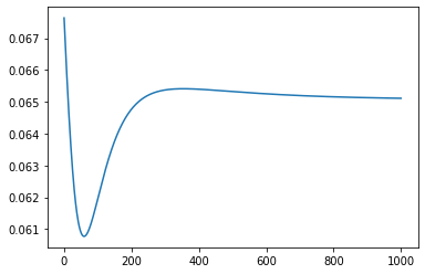
Refer to caption
(a) In above we have chosen 𝐱=(1,1,1){\mathchoice{\mbox{\boldmath$\displaystyle\bf x$}}{\mbox{\boldmath$\textstyle\bf x$}}{\mbox{\boldmath$\scriptstyle\bf x$}}{\mbox{\boldmath$\scriptscriptstyle\bf x$}}}=(1,-1,1) and
𝐱=(1.01,0.999,1.2){\mathchoice{\mbox{\boldmath$\displaystyle\bf x$}}{\mbox{\boldmath$\textstyle\bf x$}}{\mbox{\boldmath$\scriptstyle\bf x$}}{\mbox{\boldmath$\scriptscriptstyle\bf x$}}}^{\prime}=(1.01,0.999,1.2).
Refer to caption
(b) In above we have chosen 𝐱=(1,11,1){\mathchoice{\mbox{\boldmath$\displaystyle\bf x$}}{\mbox{\boldmath$\textstyle\bf x$}}{\mbox{\boldmath$\scriptstyle\bf x$}}{\mbox{\boldmath$\scriptscriptstyle\bf x$}}}=(1,-11,1) and
𝐱=(1.01,0.999,1.2){\mathchoice{\mbox{\boldmath$\displaystyle\bf x$}}{\mbox{\boldmath$\textstyle\bf x$}}{\mbox{\boldmath$\scriptstyle\bf x$}}{\mbox{\boldmath$\scriptscriptstyle\bf x$}}}^{\prime}=(1.01,0.999,1.2).
Figure 12: For θ=0.001\theta=0.001, we plot the R.H.S of equation 14 (y-axis) for t{1,2,,1000}t\in\{1,2,\ldots,1000\} (x-axis)

More interestingly, we now cast the setup of Eq. 14 as S.G.D. solving the following class of risk minimization questions,

min𝐰3𝔼(𝐱,y)[(𝐰,(𝐱,y))]\displaystyle\min_{{\mathchoice{\mbox{\boldmath$\displaystyle\bf w$}}{\mbox{\boldmath$\textstyle\bf w$}}{\mbox{\boldmath$\scriptstyle\bf w$}}{\mbox{\boldmath$\scriptscriptstyle\bf w$}}}\in\mathbb{R}^{3}}\mathbb{E}_{({\mathchoice{\mbox{\boldmath$\displaystyle\bf x$}}{\mbox{\boldmath$\textstyle\bf x$}}{\mbox{\boldmath$\scriptstyle\bf x$}}{\mbox{\boldmath$\scriptscriptstyle\bf x$}}},y)}\left[\ell({\mathchoice{\mbox{\boldmath$\displaystyle\bf w$}}{\mbox{\boldmath$\textstyle\bf w$}}{\mbox{\boldmath$\scriptstyle\bf w$}}{\mbox{\boldmath$\scriptscriptstyle\bf w$}}},({\mathchoice{\mbox{\boldmath$\displaystyle\bf x$}}{\mbox{\boldmath$\textstyle\bf x$}}{\mbox{\boldmath$\scriptstyle\bf x$}}{\mbox{\boldmath$\scriptscriptstyle\bf x$}}},y))\right]
min𝐰3𝔼𝐱𝒩(0,I3×3)[12(y(𝐱)(α(𝐱)+p=13βp,p(𝐱)wp2))2]\displaystyle\coloneqq\min_{{\mathchoice{\mbox{\boldmath$\displaystyle\bf w$}}{\mbox{\boldmath$\textstyle\bf w$}}{\mbox{\boldmath$\scriptstyle\bf w$}}{\mbox{\boldmath$\scriptscriptstyle\bf w$}}}\in\mathbb{R}^{3}}\mathbb{E}_{{\mathchoice{\mbox{\boldmath$\displaystyle\bf x$}}{\mbox{\boldmath$\textstyle\bf x$}}{\mbox{\boldmath$\scriptstyle\bf x$}}{\mbox{\boldmath$\scriptscriptstyle\bf x$}}}\mathbin{\sim}{\cal N}(0,\textrm{I}_{3\times 3})}\left[\frac{1}{2}\left(y({\mathchoice{\mbox{\boldmath$\displaystyle\bf x$}}{\mbox{\boldmath$\textstyle\bf x$}}{\mbox{\boldmath$\scriptstyle\bf x$}}{\mbox{\boldmath$\scriptscriptstyle\bf x$}}})-\left(\alpha({\mathchoice{\mbox{\boldmath$\displaystyle\bf x$}}{\mbox{\boldmath$\textstyle\bf x$}}{\mbox{\boldmath$\scriptstyle\bf x$}}{\mbox{\boldmath$\scriptscriptstyle\bf x$}}})+\sum_{p=1}^{3}\beta_{p,p}({\mathchoice{\mbox{\boldmath$\displaystyle\bf x$}}{\mbox{\boldmath$\textstyle\bf x$}}{\mbox{\boldmath$\scriptstyle\bf x$}}{\mbox{\boldmath$\scriptscriptstyle\bf x$}}})w_{p}^{2}\right)\right)^{2}\right] (15)

with βp,p(𝐱)=xp\beta_{p,p}({\mathchoice{\mbox{\boldmath$\displaystyle\bf x$}}{\mbox{\boldmath$\textstyle\bf x$}}{\mbox{\boldmath$\scriptstyle\bf x$}}{\mbox{\boldmath$\scriptscriptstyle\bf x$}}})=x_{p} for p=1,2,3p=1,2,3 as specified earlier and the true labels y(𝐱)y({\mathchoice{\mbox{\boldmath$\displaystyle\bf x$}}{\mbox{\boldmath$\textstyle\bf x$}}{\mbox{\boldmath$\scriptstyle\bf x$}}{\mbox{\boldmath$\scriptscriptstyle\bf x$}}}) being also generated as earlier y(𝐱)=α(𝐱)+𝐱,𝐰2y({\mathchoice{\mbox{\boldmath$\displaystyle\bf x$}}{\mbox{\boldmath$\textstyle\bf x$}}{\mbox{\boldmath$\scriptstyle\bf x$}}{\mbox{\boldmath$\scriptscriptstyle\bf x$}}})=\alpha({\mathchoice{\mbox{\boldmath$\displaystyle\bf x$}}{\mbox{\boldmath$\textstyle\bf x$}}{\mbox{\boldmath$\scriptstyle\bf x$}}{\mbox{\boldmath$\scriptscriptstyle\bf x$}}})+\left\langle{\mathchoice{\mbox{\boldmath$\displaystyle\bf x$}}{\mbox{\boldmath$\textstyle\bf x$}}{\mbox{\boldmath$\scriptstyle\bf x$}}{\mbox{\boldmath$\scriptscriptstyle\bf x$}}},{\mathchoice{\mbox{\boldmath$\displaystyle\bf w$}}{\mbox{\boldmath$\textstyle\bf w$}}{\mbox{\boldmath$\scriptstyle\bf w$}}{\mbox{\boldmath$\scriptscriptstyle\bf w$}}}_{*}^{2}\right\rangle with 𝐰=(1,2,3){\mathchoice{\mbox{\boldmath$\displaystyle\bf w$}}{\mbox{\boldmath$\textstyle\bf w$}}{\mbox{\boldmath$\scriptstyle\bf w$}}{\mbox{\boldmath$\scriptscriptstyle\bf w$}}}_{*}=(1,2,3).We denote (wt,1,wt,2,wt,3)=𝐰t3(w_{t,1},w_{t,2},w_{t,3})={\mathchoice{\mbox{\boldmath$\displaystyle\bf w$}}{\mbox{\boldmath$\textstyle\bf w$}}{\mbox{\boldmath$\scriptstyle\bf w$}}{\mbox{\boldmath$\scriptscriptstyle\bf w$}}}_{t}\in\mathbb{R}^{3} as the ttht^{th}-iterate of the S.G.D. We initialize the S.G.D. at w0,1=12,w0,2=2,w0,3=2w_{0,1}=\frac{1}{\sqrt{2}},w_{0,2}=\sqrt{2},w_{0,3}=2, the same initial conditions as used in deriving the O.D.E solution in equation 14 and use a step-length of η=0.001\eta=0.001 as was the value of the θ\theta parameter in the plots in Figure 12. Then the ttht^{th}- step in the S.G.D. would read,

𝐱t𝒩(0,I3×3){\mathchoice{\mbox{\boldmath$\displaystyle\bf x$}}{\mbox{\boldmath$\textstyle\bf x$}}{\mbox{\boldmath$\scriptstyle\bf x$}}{\mbox{\boldmath$\scriptscriptstyle\bf x$}}}_{t}\mathbin{\sim}{\cal N}(0,\textrm{I}_{3\times 3})
𝐰t+1=𝐰t+2η(p=13xt,p(𝐰,p2𝐰t,p2))𝐱t𝐰t{\mathchoice{\mbox{\boldmath$\displaystyle\bf w$}}{\mbox{\boldmath$\textstyle\bf w$}}{\mbox{\boldmath$\scriptstyle\bf w$}}{\mbox{\boldmath$\scriptscriptstyle\bf w$}}}_{t+1}={\mathchoice{\mbox{\boldmath$\displaystyle\bf w$}}{\mbox{\boldmath$\textstyle\bf w$}}{\mbox{\boldmath$\scriptstyle\bf w$}}{\mbox{\boldmath$\scriptscriptstyle\bf w$}}}_{t}+2\eta\left(\sum_{p=1}^{3}x_{t,p}({\mathchoice{\mbox{\boldmath$\displaystyle\bf w$}}{\mbox{\boldmath$\textstyle\bf w$}}{\mbox{\boldmath$\scriptstyle\bf w$}}{\mbox{\boldmath$\scriptscriptstyle\bf w$}}}_{*,p}^{2}-{\mathchoice{\mbox{\boldmath$\displaystyle\bf w$}}{\mbox{\boldmath$\textstyle\bf w$}}{\mbox{\boldmath$\scriptstyle\bf w$}}{\mbox{\boldmath$\scriptscriptstyle\bf w$}}}_{t,p}^{2})\right){\mathchoice{\mbox{\boldmath$\displaystyle\bf x$}}{\mbox{\boldmath$\textstyle\bf x$}}{\mbox{\boldmath$\scriptstyle\bf x$}}{\mbox{\boldmath$\scriptscriptstyle\bf x$}}}_{t}\odot{\mathchoice{\mbox{\boldmath$\displaystyle\bf w$}}{\mbox{\boldmath$\textstyle\bf w$}}{\mbox{\boldmath$\scriptstyle\bf w$}}{\mbox{\boldmath$\scriptscriptstyle\bf w$}}}_{t}

Thus at every 𝐰t{\mathchoice{\mbox{\boldmath$\displaystyle\bf w$}}{\mbox{\boldmath$\textstyle\bf w$}}{\mbox{\boldmath$\scriptstyle\bf w$}}{\mbox{\boldmath$\scriptscriptstyle\bf w$}}}_{t} for the above algorithm we can compute Srel(𝐱,𝐱)S_{\rm rel}({\mathchoice{\mbox{\boldmath$\displaystyle\bf x$}}{\mbox{\boldmath$\textstyle\bf x$}}{\mbox{\boldmath$\scriptstyle\bf x$}}{\mbox{\boldmath$\scriptscriptstyle\bf x$}}},{\mathchoice{\mbox{\boldmath$\displaystyle\bf x$}}{\mbox{\boldmath$\textstyle\bf x$}}{\mbox{\boldmath$\scriptstyle\bf x$}}{\mbox{\boldmath$\scriptscriptstyle\bf x$}}}^{\prime}) as given in Definition 1 with (𝐰t,(𝐱,y))\ell({\mathchoice{\mbox{\boldmath$\displaystyle\bf w$}}{\mbox{\boldmath$\textstyle\bf w$}}{\mbox{\boldmath$\scriptstyle\bf w$}}{\mbox{\boldmath$\scriptscriptstyle\bf w$}}}_{t},({\mathchoice{\mbox{\boldmath$\displaystyle\bf x$}}{\mbox{\boldmath$\textstyle\bf x$}}{\mbox{\boldmath$\scriptstyle\bf x$}}{\mbox{\boldmath$\scriptscriptstyle\bf x$}}},y)) as given in Definition 15. For the 𝐱&𝐱{\mathchoice{\mbox{\boldmath$\displaystyle\bf x$}}{\mbox{\boldmath$\textstyle\bf x$}}{\mbox{\boldmath$\scriptstyle\bf x$}}{\mbox{\boldmath$\scriptscriptstyle\bf x$}}}~\&~{\mathchoice{\mbox{\boldmath$\displaystyle\bf x$}}{\mbox{\boldmath$\textstyle\bf x$}}{\mbox{\boldmath$\scriptstyle\bf x$}}{\mbox{\boldmath$\scriptscriptstyle\bf x$}}}^{\prime} as in Figure 12, in Figure 13 we give the corresponding plots averaged over many samples of S.G.D. runs - and in all these samples the iterates were all eventually satisfying the condition 𝐰t𝐰<106\norm{\w_t - \w_*}<10^{-6}.

Refer to caption
(a) In above we have chosen 𝐱=(1,1,1){\mathchoice{\mbox{\boldmath$\displaystyle\bf x$}}{\mbox{\boldmath$\textstyle\bf x$}}{\mbox{\boldmath$\scriptstyle\bf x$}}{\mbox{\boldmath$\scriptscriptstyle\bf x$}}}=(1,-1,1)
and 𝐱=(1.01,0.999,1.2){\mathchoice{\mbox{\boldmath$\displaystyle\bf x$}}{\mbox{\boldmath$\textstyle\bf x$}}{\mbox{\boldmath$\scriptstyle\bf x$}}{\mbox{\boldmath$\scriptscriptstyle\bf x$}}}^{\prime}=(1.01,0.999,1.2)
Refer to caption
(b) In above we have chosen 𝐱=(1,11,1){\mathchoice{\mbox{\boldmath$\displaystyle\bf x$}}{\mbox{\boldmath$\textstyle\bf x$}}{\mbox{\boldmath$\scriptstyle\bf x$}}{\mbox{\boldmath$\scriptscriptstyle\bf x$}}}=(1,-11,1)
and 𝐱=(1.01,0.999,1.2){\mathchoice{\mbox{\boldmath$\displaystyle\bf x$}}{\mbox{\boldmath$\textstyle\bf x$}}{\mbox{\boldmath$\scriptstyle\bf x$}}{\mbox{\boldmath$\scriptscriptstyle\bf x$}}}^{\prime}=(1.01,0.999,1.2)
Figure 13: We plot SrelS_{\rm rel} for the ttht^{th}-iterate of S.G.D. training on the risk given in equation 15 for t{1,2,,2000}t\in\{1,2,\ldots,2000\} and using step-length of η=0.001\eta=0.001. The plotted value is an average over multiple samples of S.G.D. runs. (The reader is urged to note the similarity in the hyper-parameter settings and the eventual similarity of the plots as in Figures 12)

The sharp resemblance (of values as well as of the shape) between Figures 12 and 13, justifies our approach of modelling the behaviour of local elasticity for realistic training algorithms like S.G.D. via appropriate limits of solutions of certain O.D.Es.  

For certain set of special cases of equation 13, in the next theorem we shall prove some of the key features observed in these two figures.

Theorem 5.3 (A Special Symmetric Case with 22 Features in 22 dimensions).

Suppose there are 2 features β1,β2:22\beta_{1},\beta_{2}:\mathbb{R}^{2}\rightarrow\mathbb{R}^{2} and we are considering the following predictor class,

2×2(𝐰,𝐱)f2,2,lin(𝐰,𝐱)α(𝐱)+r=12βr,r(𝐱)wr2\begin{split}\mathbb{R}^{2}\times\mathbb{R}^{2}\ni({\mathchoice{\mbox{\boldmath$\displaystyle\bf w$}}{\mbox{\boldmath$\textstyle\bf w$}}{\mbox{\boldmath$\scriptstyle\bf w$}}{\mbox{\boldmath$\scriptscriptstyle\bf w$}}},{\mathchoice{\mbox{\boldmath$\displaystyle\bf x$}}{\mbox{\boldmath$\textstyle\bf x$}}{\mbox{\boldmath$\scriptstyle\bf x$}}{\mbox{\boldmath$\scriptscriptstyle\bf x$}}})\mapsto f_{\rm 2,2,lin}({\mathchoice{\mbox{\boldmath$\displaystyle\bf w$}}{\mbox{\boldmath$\textstyle\bf w$}}{\mbox{\boldmath$\scriptstyle\bf w$}}{\mbox{\boldmath$\scriptscriptstyle\bf w$}}},{\mathchoice{\mbox{\boldmath$\displaystyle\bf x$}}{\mbox{\boldmath$\textstyle\bf x$}}{\mbox{\boldmath$\scriptstyle\bf x$}}{\mbox{\boldmath$\scriptscriptstyle\bf x$}}})\coloneqq\alpha({\mathchoice{\mbox{\boldmath$\displaystyle\bf x$}}{\mbox{\boldmath$\textstyle\bf x$}}{\mbox{\boldmath$\scriptstyle\bf x$}}{\mbox{\boldmath$\scriptscriptstyle\bf x$}}})+\sum_{r=1}^{2}\beta_{r,r}({\mathchoice{\mbox{\boldmath$\displaystyle\bf x$}}{\mbox{\boldmath$\textstyle\bf x$}}{\mbox{\boldmath$\scriptstyle\bf x$}}{\mbox{\boldmath$\scriptscriptstyle\bf x$}}})\cdot w_{r}^{2}\in\mathbb{R}\end{split} (16)

We assume the data-distribution over 2×\mathbb{R}^{2}\times\mathbb{R} to be s.t the following are finite : bi𝔼(𝐱,y)[βi,i(𝐱)2],i=1,2b_{i}\coloneqq\mathbb{E}_{({\mathchoice{\mbox{\boldmath$\displaystyle\bf x$}}{\mbox{\boldmath$\textstyle\bf x$}}{\mbox{\boldmath$\scriptstyle\bf x$}}{\mbox{\boldmath$\scriptscriptstyle\bf x$}}},y)}\left[\beta_{i,i}({\mathchoice{\mbox{\boldmath$\displaystyle\bf x$}}{\mbox{\boldmath$\textstyle\bf x$}}{\mbox{\boldmath$\scriptstyle\bf x$}}{\mbox{\boldmath$\scriptscriptstyle\bf x$}}})^{2}\right],~\forall i=1,2 and 0<ai𝔼(𝐱,y)[(yα(𝐱))βi,i(𝐱)],i=1,20<a_{i}\coloneqq\mathbb{E}_{({\mathchoice{\mbox{\boldmath$\displaystyle\bf x$}}{\mbox{\boldmath$\textstyle\bf x$}}{\mbox{\boldmath$\scriptstyle\bf x$}}{\mbox{\boldmath$\scriptscriptstyle\bf x$}}},y)}\left[(y-\alpha({\mathchoice{\mbox{\boldmath$\displaystyle\bf x$}}{\mbox{\boldmath$\textstyle\bf x$}}{\mbox{\boldmath$\scriptstyle\bf x$}}{\mbox{\boldmath$\scriptscriptstyle\bf x$}}}))\beta_{i,i}({\mathchoice{\mbox{\boldmath$\displaystyle\bf x$}}{\mbox{\boldmath$\textstyle\bf x$}}{\mbox{\boldmath$\scriptstyle\bf x$}}{\mbox{\boldmath$\scriptscriptstyle\bf x$}}})\right],~\forall i=1,2 Further suppose that α,β{0}\exists~\alpha,\beta\in\mathbb{R}\setminus\{0\} s.t,

b1a1=b2a2=α2,b1a1+1w1(0)2=b2a2+1w2(0)2=β2\frac{b_{1}}{a_{1}}=\frac{b_{2}}{a_{2}}=\alpha^{2},\quad-\frac{b_{1}}{a_{1}}+\frac{1}{w_{1}(0)^{2}}=-\frac{b_{2}}{a_{2}}+\frac{1}{w_{2}(0)^{2}}=\beta^{2}

And we suppose the following condition on the features at the point 𝐱\textstyle\bf x and 𝐱{\mathchoice{\mbox{\boldmath$\displaystyle\bf x$}}{\mbox{\boldmath$\textstyle\bf x$}}{\mbox{\boldmath$\scriptstyle\bf x$}}{\mbox{\boldmath$\scriptscriptstyle\bf x$}}}^{\prime} being considered,

|β1,1(𝐱)β1,1(𝐱)+β2,2(𝐱)β2,2(𝐱)||β1,1(𝐱)2+β2,2(𝐱)2|>0\frac{\absolutevalue{\beta_{1,1}(\x') \beta_{1,1}(\x) + \beta_{2,2}(\x') \beta_{2,2}(\x)}}{\absolutevalue{\beta_{1,1}(\x)^2 + \beta_{2,2}(\x')^2}}>0

Then t\exists t^{*} s.t tt\forall t\geq t^{*}, limη0[Srel]𝐱,𝐱\lim_{\eta\rightarrow 0}[S_{\rm rel}]_{{\mathchoice{\mbox{\boldmath$\displaystyle\bf x$}}{\mbox{\boldmath$\textstyle\bf x$}}{\mbox{\boldmath$\scriptstyle\bf x$}}{\mbox{\boldmath$\scriptscriptstyle\bf x$}}}^{\prime},{\mathchoice{\mbox{\boldmath$\displaystyle\bf x$}}{\mbox{\boldmath$\textstyle\bf x$}}{\mbox{\boldmath$\scriptstyle\bf x$}}{\mbox{\boldmath$\scriptscriptstyle\bf x$}}}} (as defined via equations 10 and 11) is always bounded away from 00 and this lower bound is monotonically increasing with tt.

The proof of the above theorem can be found in Appendix C.3. We note that the above result can be seen as a partial evidence towards the property envisaged in Hypothesis 1.2.

Remark.

For intuition consider a special case of the above with 𝛃i,i(𝐳)=zi,i={1,2}\boldsymbol{\beta}_{i,i}({\mathchoice{\mbox{\boldmath$\displaystyle\bf z$}}{\mbox{\boldmath$\textstyle\bf z$}}{\mbox{\boldmath$\scriptstyle\bf z$}}{\mbox{\boldmath$\scriptscriptstyle\bf z$}}})=z_{i},~\forall i=\{1,2\}. Then we can write,

|β1,1(𝐱)β1,1(𝐱)+β2,2(𝐱)β2,2(𝐱)||β1,1(𝐱)2+β2,2(𝐱)2|=|x1x1+x2x2||x12+x22|=|𝐱,𝐱|𝐱2\frac{\absolutevalue{\beta_{1,1}(\x') \beta_{1,1}(\x) + \beta_{2,2}(\x') \beta_{2,2}(\x)}}{\absolutevalue{\beta_{1,1}(\x)^2 + \beta_{2,2}(\x')^2}}=\frac{\absolutevalue{x'_1x_1 + x'_2x_2}}{\absolutevalue{x_1^2 + x_2^2}}=\frac{\absolutevalue{\ip{\x'}{\x}}}{\norm{\x}^{2}}

Hence in this case the condition reduces to 𝐱{\mathchoice{\mbox{\boldmath$\displaystyle\bf x$}}{\mbox{\boldmath$\textstyle\bf x$}}{\mbox{\boldmath$\scriptstyle\bf x$}}{\mbox{\boldmath$\scriptscriptstyle\bf x$}}}^{\prime} not being orthogonal to 𝐱\textstyle\bf x for the the SrelS_{\rm rel} to be prevented from being arbitrarily low.

6 Conclusion

In this work we were able to demonstrate via theory and neural experiments, a general phenomenon that the weight updates in many popular training setups cause prediction changes preferably for those data which are “related” to the point being sampled for computing the stochastic gradient. And very crucially - and possibly surprisingly - our experiments in the classification setup showed that this preference sets in very early on in the training - much before the asymptotic classification accuracies have been attained. We recall that to pin down the above effect we had to introduce a new definition of “local elasticity” (Definition 3) which measures the changes in the predicted distribution over classes (for a fixed input) while the training is underway.

One of the main next steps from here on is to develop theoretical models where one can reproduce the phenomenon of local elasticity with neural classification experiments as demonstrated in Section 2.1. More generally, it would be an exciting avenue of future research to identify learning scenarios where the extended idea of SrelS_{\rm rel} as given in Definition 3 can be exactly calculated and thus be able to rigorously establish its interesting properties demonstrated in the experiments. Lastly, a necessary and sufficient condition on a learning process doing regression remains to be identified for which one can rigorously prove the late time non-decreasing behavior of SrelS_{\rm rel}.

7 Acknowledgements

We would like to thank Weijie Su, Hangfeng He, Jiayao Zhang, Danny Wood and Neil Walton for various discussions while writing this paper. Anirbit Mukherjee would like to thank Wharton Dean’s Fund for Postdoctoral Research and Weijie Su’s NSF CAREER DMS-1847415 for funding this research.

References

  • [KH+09] Alex Krizhevsky and Geoffrey Hinton “Learning multiple layers of features from tiny images” Citeseer, 2009
  • [Net+11] Yuval Netzer et al. “Reading digits in natural images with unsupervised feature learning”, 2011
  • [Lee+17] Jaehoon Lee et al. “Deep Neural Networks as Gaussian Processes”, 2017 arXiv:1711.00165 [stat.ML]
  • [PL17] Tomaso Poggio and Qianli Liao “Theory II: Landscape of the Empirical Risk in Deep Learning” In arXiv preprint arXiv:1703.09833, 2017
  • [Sil+17] David Silver et al. “Mastering the game of Go without human knowledge” In Nature 550.7676 Nature Research, 2017, pp. 354–359
  • [Zha+17] Chiyuan Zhang et al. “Theory of Deep Learning III: Generalization Properties of SGD”, 2017
  • [Che+18] Hongming Chen et al. “The rise of deep learning in drug discovery” In Drug discovery today 23.6 Elsevier, 2018, pp. 1241–1250
  • [Du+18] Simon. Du et al. “Gradient Descent Finds Global Minima of Deep Neural Networks”, 2018 arXiv:1811.03804 [cs.LG]
  • [GKM18] Surbhi Goel, Adam Klivans and Raghu Meka “Learning one convolutional layer with overlapping patches” In arXiv preprint arXiv:1802.02547, 2018
  • [SPW18] Marwin Segler, Mike Preuss and Mark Waller “Planning chemical syntheses with deep neural networks and symbolic AI” In Nature 555.7698 Nature Publishing Group, 2018, pp. 604–610
  • [Sil+18] David Silver et al. “A general reinforcement learning algorithm that masters chess, shogi, and Go through self-play” In Science 362.6419 American Association for the Advancement of Science, 2018, pp. 1140–1144
  • [Zou+18] Difan Zou, Yuan Cao, Dongruo Zhou and Quanquan Gu “Stochastic gradient descent optimizes over-parameterized deep relu networks” In arXiv preprint arXiv:1811.08888, 2018
  • [AL19] Zeyuan Allen-Zhu and Yuanzhi Li “What Can ResNet Learn Efficiently, Going Beyond Kernels?” In Advances in Neural Information Processing Systems, 2019, pp. 9015–9025
  • [ALL19] Zeyuan Allen-Zhu, Yuanzhi Li and Yingyu Liang “Learning and generalization in overparameterized neural networks, going beyond two layers” In Advances in neural information processing systems, 2019, pp. 6155–6166
  • [ALS19] Zeyuan Allen-Zhu, Yuanzhi Li and Zhao Song “A Convergence Theory for Deep Learning via Over-Parameterization” In International Conference on Machine Learning, 2019, pp. 242–252
  • [ALS19a] Zeyuan Allen-Zhu, Yuanzhi Li and Zhao Song “On the convergence rate of training recurrent neural networks” In Advances in Neural Information Processing Systems, 2019, pp. 6673–6685
  • [Aro+19] Sanjeev Arora et al. “Fine-Grained Analysis of Optimization and Generalization for Overparameterized Two-Layer Neural Networks” In International Conference on Machine Learning, 2019, pp. 322–332
  • [Aro+19a] Sanjeev Arora et al. “On exact computation with an infinitely wide neural net” In Advances in Neural Information Processing Systems, 2019, pp. 8139–8148
  • [BL19] Yu Bai and Jason Lee “Beyond Linearization: On Quadratic and Higher-Order Approximation of Wide Neural Networks” In International Conference on Learning Representations, 2019
  • [FNN19] Stanislav Fort, Pawel Nowak and Srini Narayanan “Stiffness: A New Perspective on Generalization in Neural Networks” In CoRR abs/1901.09491, 2019 arXiv: http://arxiv.org/abs/1901.09491
  • [GKK19] Surbhi Goel, Sushrut Karmalkar and Adam Klivans “Time/accuracy tradeoffs for learning a relu with respect to gaussian marginals” In Advances in Neural Information Processing Systems, 2019, pp. 8584–8593
  • [HS19] Hangfeng He and Weijie Su “The Local Elasticity of Neural Networks” In International Conference on Learning Representations, 2019
  • [HY19] Jiaoyang Huang and Horng-Tzer Yau “Dynamics of deep neural networks and neural tangent hierarchy” In arXiv preprint arXiv:1909.08156, 2019
  • [Lee+19] Jaehoon Lee et al. “Wide neural networks of any depth evolve as linear models under gradient descent” In Advances in neural information processing systems 32, 2019, pp. 8572–8583
  • [SY19] Lili Su and Pengkun Yang “On Learning Over-parameterized Neural Networks: A Functional Approximation Perspective” In Advances in Neural Information Processing Systems, 2019, pp. 2637–2646
  • [Wei+19] Colin Wei, Jason Lee, Qiang Liu and Tengyu Ma “Regularization matters: Generalization and optimization of neural nets vs their induced kernel” In Advances in Neural Information Processing Systems, 2019, pp. 9709–9721
  • [WDW19] Xiaoxia Wu, Simon Du and Rachel Ward “Global convergence of adaptive gradient methods for an over-parameterized neural network” In arXiv preprint arXiv:1902.07111, 2019
  • [ZG19] Difan Zou and Quanquan Gu “An improved analysis of training over-parameterized deep neural networks” In Advances in Neural Information Processing Systems, 2019, pp. 2053–2062
  • [Cha20] Satrajit Chatterjee “Coherent Gradients: An Approach to Understanding Generalization in Gradient Descent-based Optimization” In CoRR abs/2002.10657, 2020 arXiv: https://arxiv.org/abs/2002.10657
  • [CHS20] Shuxiao Chen, Hangfeng He and Weijie Su “Label-Aware Neural Tangent Kernel: Toward Better Generalization and Local Elasticity” In Advances in Neural Information Processing Systems 33, 2020
  • [Dal+20] Mogens Dalgaard, Felix Motzoi, Jens Sørensen and Jacob Sherson “Global optimization of quantum dynamics with AlphaZero deep exploration” In npj Quantum Information 6.1 Nature Publishing Group, 2020, pp. 1–9
  • [DHS20] Zhun Deng, Hangfeng He and Weijie. Su “Toward Better Generalization Bounds with Locally Elastic Stability” In CoRR abs/2010.13988, 2020 arXiv: https://arxiv.org/abs/2010.13988
  • [Dia+20] Ilias Diakonikolas et al. “Approximation Schemes for ReLU Regression” In Conference on Learning Theory, 2020
  • [FCG20] Spencer Frei, Yuan Cao and Quanquan Gu “Agnostic Learning of a Single Neuron with Gradient Descent” In arXiv preprint arXiv:2005.14426, 2020
  • [Muk20] Anirbit Mukherjee “A Study Of The Mathematics Of Deep Learning”, 2020
  • [Sch+20] Julian Schrittwieser et al. “Mastering atari, go, chess and shogi by planning with a learned model” In Nature 588.7839 Nature Publishing Group, 2020, pp. 604–609
  • [Woo+20] Blake Woodworth et al. “Kernel and rich regimes in overparametrized models” In Conference on Learning Theory, 2020, pp. 3635–3673 PMLR
  • [Fan+21] Cong Fang, Hangfeng He, Qi Long and Weijie. Su “Layer-Peeled Model: Toward Understanding Well-Trained Deep Neural Networks” In CoRR abs/2101.12699, 2021 arXiv: https://arxiv.org/abs/2101.12699
  • [GM22] Pulkit Gopalani and Anirbit Mukherjee “ Global Convergence of SGD On Two Layer Neural Nets”, 2022 URL: https://doi.org/10.48550/arXiv.2210.11452
  • [KM22] Sayar Karmakar and Anirbit Mukherjee “Provable training of a ReLU gate with an iterative non-gradient algorithm” In Neural Networks 151, 2022, pp. 264–275 DOI: https://doi.org/10.1016/j.neunet.2022.03.040
  • [MPP22] Dustin. Mixon, Hans Parshall and Jianzong Pi “Neural collapse with unconstrained features” In Sampling Theory, Signal Processing, and Data Analysis 20.2, 2022, pp. 11 DOI: 10.1007/s43670-022-00027-5
  • [KMP23] Sayar Karmakar, Anirbit Mukherjee and Theodore Papamarkou “ Depth-2 neural networks under a data-poisoning attack” In Neurocomputing 532, 2023, pp. 56–66 DOI: https://doi.org/10.1016/j.neucom.2023.02.034

Appendix A Proofs of Section 3

A.1 Proof of Theorem 3.1

Proof.

We note by directly differentiating the given evolution equation,

𝐰q(t)=eθ2𝐌t(𝐰q(0)β2𝐌1𝐮q)+β2𝐌1𝐮qd𝐰qdt=(θ2𝐌)eθ2𝐌t(𝐰q(0)β2𝐌1𝐮q)=θ2𝐌eθ2𝐌t𝐰q(0)+θ2β2eθ2𝐌t𝐮q=θ2𝐌(𝐰q+β2𝐌1eθ2𝐌t𝐮qβ2𝐌1𝐮q)++θ2β2eθ2𝐌t𝐮q=θ2𝐌𝐰q+θ2β2𝐮q\begin{split}{\mathchoice{\mbox{\boldmath$\displaystyle\bf w$}}{\mbox{\boldmath$\textstyle\bf w$}}{\mbox{\boldmath$\scriptstyle\bf w$}}{\mbox{\boldmath$\scriptscriptstyle\bf w$}}}_{q}(t)&=e^{-\theta^{2}\mathbf{M}t}\left({\mathchoice{\mbox{\boldmath$\displaystyle\bf w$}}{\mbox{\boldmath$\textstyle\bf w$}}{\mbox{\boldmath$\scriptstyle\bf w$}}{\mbox{\boldmath$\scriptscriptstyle\bf w$}}}_{q}(0)-\beta^{2}\mathbf{M}^{-1}{\mathchoice{\mbox{\boldmath$\displaystyle\bf u$}}{\mbox{\boldmath$\textstyle\bf u$}}{\mbox{\boldmath$\scriptstyle\bf u$}}{\mbox{\boldmath$\scriptscriptstyle\bf u$}}}_{q}\right)+\beta^{2}\mathbf{M}^{-1}{\mathchoice{\mbox{\boldmath$\displaystyle\bf u$}}{\mbox{\boldmath$\textstyle\bf u$}}{\mbox{\boldmath$\scriptstyle\bf u$}}{\mbox{\boldmath$\scriptscriptstyle\bf u$}}}_{q}\\ \Longrightarrow\derivative{\w_q}{t}&=(-\theta^{2}\mathbf{M})e^{-\theta^{2}\mathbf{M}t}\left({\mathchoice{\mbox{\boldmath$\displaystyle\bf w$}}{\mbox{\boldmath$\textstyle\bf w$}}{\mbox{\boldmath$\scriptstyle\bf w$}}{\mbox{\boldmath$\scriptscriptstyle\bf w$}}}_{q}(0)-\beta^{2}\mathbf{M}^{-1}{\mathchoice{\mbox{\boldmath$\displaystyle\bf u$}}{\mbox{\boldmath$\textstyle\bf u$}}{\mbox{\boldmath$\scriptstyle\bf u$}}{\mbox{\boldmath$\scriptscriptstyle\bf u$}}}_{q}\right)\\ &=-\theta^{2}\mathbf{M}e^{-\theta^{2}\mathbf{M}t}{\mathchoice{\mbox{\boldmath$\displaystyle\bf w$}}{\mbox{\boldmath$\textstyle\bf w$}}{\mbox{\boldmath$\scriptstyle\bf w$}}{\mbox{\boldmath$\scriptscriptstyle\bf w$}}}_{q}(0)+\theta^{2}\beta^{2}e^{-\theta^{2}\mathbf{M}t}{\mathchoice{\mbox{\boldmath$\displaystyle\bf u$}}{\mbox{\boldmath$\textstyle\bf u$}}{\mbox{\boldmath$\scriptstyle\bf u$}}{\mbox{\boldmath$\scriptscriptstyle\bf u$}}}_{q}\\ &=-\theta^{2}\mathbf{M}({\mathchoice{\mbox{\boldmath$\displaystyle\bf w$}}{\mbox{\boldmath$\textstyle\bf w$}}{\mbox{\boldmath$\scriptstyle\bf w$}}{\mbox{\boldmath$\scriptscriptstyle\bf w$}}}_{q}+\beta^{2}\mathbf{M}^{-1}e^{-\theta^{2}\mathbf{M}t}{\mathchoice{\mbox{\boldmath$\displaystyle\bf u$}}{\mbox{\boldmath$\textstyle\bf u$}}{\mbox{\boldmath$\scriptstyle\bf u$}}{\mbox{\boldmath$\scriptscriptstyle\bf u$}}}_{q}-\beta^{2}\mathbf{M}^{-1}{\mathchoice{\mbox{\boldmath$\displaystyle\bf u$}}{\mbox{\boldmath$\textstyle\bf u$}}{\mbox{\boldmath$\scriptstyle\bf u$}}{\mbox{\boldmath$\scriptscriptstyle\bf u$}}}_{q})++\theta^{2}\beta^{2}e^{-\theta^{2}\mathbf{M}t}{\mathchoice{\mbox{\boldmath$\displaystyle\bf u$}}{\mbox{\boldmath$\textstyle\bf u$}}{\mbox{\boldmath$\scriptstyle\bf u$}}{\mbox{\boldmath$\scriptscriptstyle\bf u$}}}_{q}\\ &=-\theta^{2}\mathbf{M}{\mathchoice{\mbox{\boldmath$\displaystyle\bf w$}}{\mbox{\boldmath$\textstyle\bf w$}}{\mbox{\boldmath$\scriptstyle\bf w$}}{\mbox{\boldmath$\scriptscriptstyle\bf w$}}}_{q}+\theta^{2}\beta^{2}{\mathchoice{\mbox{\boldmath$\displaystyle\bf u$}}{\mbox{\boldmath$\textstyle\bf u$}}{\mbox{\boldmath$\scriptstyle\bf u$}}{\mbox{\boldmath$\scriptscriptstyle\bf u$}}}_{q}\end{split} (17)

Thus, the statement in Theorem 3.1 follows. ∎

Appendix B Proofs of Section 4

B.1 Proof of Lemma 4.2

Proof.
|max{0,𝐰+(t),𝐱}max{0,𝐰(t),𝐱}|=|max{0,𝐰(t),𝐱+ηβ𝟙{𝐰𝐱>0}[max{0,𝐰𝐱}𝐰(t)𝐱]𝐱,𝐱}max{0,𝐰(t),𝐱}|ηβ𝟙{𝐰,𝐱>0}|𝐱,𝐱||max{0,𝐰𝐱}𝐰(t)𝐱|ηβ𝟙{𝐰,𝐱>0}|𝐱,𝐱||max{0,𝐰𝐱}eβ𝐌t𝐰(0),𝐱𝐰,𝐱+eβ𝐌t𝐰,𝐱|ηβ𝟙{𝐰,𝐱>0}|𝐱,𝐱||eβ𝐌t(𝐰(0)𝐰),𝐱|\begin{split}&\absolutevalue{ \max\{0, \ip{\w^+(t)}{\x'} \} - \max\{ 0, \ip{\w(t)}{\x'} \} }\\ =&\big|\max\{0,\left\langle{\mathchoice{\mbox{\boldmath$\displaystyle\bf w$}}{\mbox{\boldmath$\textstyle\bf w$}}{\mbox{\boldmath$\scriptstyle\bf w$}}{\mbox{\boldmath$\scriptscriptstyle\bf w$}}}(t),{\mathchoice{\mbox{\boldmath$\displaystyle\bf x$}}{\mbox{\boldmath$\textstyle\bf x$}}{\mbox{\boldmath$\scriptstyle\bf x$}}{\mbox{\boldmath$\scriptscriptstyle\bf x$}}}\right\rangle+\eta\beta\mathds{1}_{\left\{{\mathchoice{\mbox{\boldmath$\displaystyle\bf w$}}{\mbox{\boldmath$\textstyle\bf w$}}{\mbox{\boldmath$\scriptstyle\bf w$}}{\mbox{\boldmath$\scriptscriptstyle\bf w$}}}_{*}^{\top}{\mathchoice{\mbox{\boldmath$\displaystyle\bf x$}}{\mbox{\boldmath$\textstyle\bf x$}}{\mbox{\boldmath$\scriptstyle\bf x$}}{\mbox{\boldmath$\scriptscriptstyle\bf x$}}}>0\right\}}\left[\max\{0,{\mathchoice{\mbox{\boldmath$\displaystyle\bf w$}}{\mbox{\boldmath$\textstyle\bf w$}}{\mbox{\boldmath$\scriptstyle\bf w$}}{\mbox{\boldmath$\scriptscriptstyle\bf w$}}}_{*}^{\top}{\mathchoice{\mbox{\boldmath$\displaystyle\bf x$}}{\mbox{\boldmath$\textstyle\bf x$}}{\mbox{\boldmath$\scriptstyle\bf x$}}{\mbox{\boldmath$\scriptscriptstyle\bf x$}}}\}-{\mathchoice{\mbox{\boldmath$\displaystyle\bf w$}}{\mbox{\boldmath$\textstyle\bf w$}}{\mbox{\boldmath$\scriptstyle\bf w$}}{\mbox{\boldmath$\scriptscriptstyle\bf w$}}}(t)^{\top}{\mathchoice{\mbox{\boldmath$\displaystyle\bf x$}}{\mbox{\boldmath$\textstyle\bf x$}}{\mbox{\boldmath$\scriptstyle\bf x$}}{\mbox{\boldmath$\scriptscriptstyle\bf x$}}}\right]\left\langle{\mathchoice{\mbox{\boldmath$\displaystyle\bf x$}}{\mbox{\boldmath$\textstyle\bf x$}}{\mbox{\boldmath$\scriptstyle\bf x$}}{\mbox{\boldmath$\scriptscriptstyle\bf x$}}},{\mathchoice{\mbox{\boldmath$\displaystyle\bf x$}}{\mbox{\boldmath$\textstyle\bf x$}}{\mbox{\boldmath$\scriptstyle\bf x$}}{\mbox{\boldmath$\scriptscriptstyle\bf x$}}}^{\prime}\right\rangle\}\\ &-\max\{0,\left\langle{\mathchoice{\mbox{\boldmath$\displaystyle\bf w$}}{\mbox{\boldmath$\textstyle\bf w$}}{\mbox{\boldmath$\scriptstyle\bf w$}}{\mbox{\boldmath$\scriptscriptstyle\bf w$}}}(t),{\mathchoice{\mbox{\boldmath$\displaystyle\bf x$}}{\mbox{\boldmath$\textstyle\bf x$}}{\mbox{\boldmath$\scriptstyle\bf x$}}{\mbox{\boldmath$\scriptscriptstyle\bf x$}}}^{\prime}\right\rangle\}\big|\\ \leq&\eta\beta\mathds{1}_{\left\{\left\langle{\mathchoice{\mbox{\boldmath$\displaystyle\bf w$}}{\mbox{\boldmath$\textstyle\bf w$}}{\mbox{\boldmath$\scriptstyle\bf w$}}{\mbox{\boldmath$\scriptscriptstyle\bf w$}}}_{*},{\mathchoice{\mbox{\boldmath$\displaystyle\bf x$}}{\mbox{\boldmath$\textstyle\bf x$}}{\mbox{\boldmath$\scriptstyle\bf x$}}{\mbox{\boldmath$\scriptscriptstyle\bf x$}}}\right\rangle>0\right\}}\absolutevalue{\ip{\x}{\x'}}\absolutevalue{\max\{0, \w_*^\top\x\} - \w(t)^\top\x}\\ \leq&\eta\beta\mathds{1}_{\left\{\left\langle{\mathchoice{\mbox{\boldmath$\displaystyle\bf w$}}{\mbox{\boldmath$\textstyle\bf w$}}{\mbox{\boldmath$\scriptstyle\bf w$}}{\mbox{\boldmath$\scriptscriptstyle\bf w$}}}_{*},{\mathchoice{\mbox{\boldmath$\displaystyle\bf x$}}{\mbox{\boldmath$\textstyle\bf x$}}{\mbox{\boldmath$\scriptstyle\bf x$}}{\mbox{\boldmath$\scriptscriptstyle\bf x$}}}\right\rangle>0\right\}}\absolutevalue{\ip{\x}{\x'}}\cdot\\ &\absolutevalue{\max\{0, \w_*^\top\x\} - \ip{e^{-\beta\M t }\w(0)}{\x} - \ip{\w_*}{\x} + \ip{e^{-\beta\M t}\w_*}{\x} }\\ \leq&\eta\beta\mathds{1}_{\left\{\left\langle{\mathchoice{\mbox{\boldmath$\displaystyle\bf w$}}{\mbox{\boldmath$\textstyle\bf w$}}{\mbox{\boldmath$\scriptstyle\bf w$}}{\mbox{\boldmath$\scriptscriptstyle\bf w$}}}_{*},{\mathchoice{\mbox{\boldmath$\displaystyle\bf x$}}{\mbox{\boldmath$\textstyle\bf x$}}{\mbox{\boldmath$\scriptstyle\bf x$}}{\mbox{\boldmath$\scriptscriptstyle\bf x$}}}\right\rangle>0\right\}}\absolutevalue{\ip{\x}{\x'}}\absolutevalue{\ip{e^{-\beta\M t }(\w(0)-\w_*)}{\x}}\end{split} (18)

B.2 Proof of Theorem 4.3

Proof.

Starting similarly as in the above proof we see that,

𝐰+(t),𝐱=𝐰(t),𝐱+ηβ𝟙{𝐰𝐱>0}[𝐰𝐰(t)]𝐱𝐱,𝐱=𝐰(t),𝐱+ηβ𝟙{𝐰𝐱>0}[eβ𝐌t(𝐰𝐰(0))]𝐱𝐱,𝐱=𝐰,𝐱+eβ𝐌t(𝐰(0)𝐰),𝐱+ηβ𝟙{𝐰𝐱>0}[eβ𝐌t(𝐰𝐰(0))]𝐱𝐱,𝐱\begin{split}\left\langle{\mathchoice{\mbox{\boldmath$\displaystyle\bf w$}}{\mbox{\boldmath$\textstyle\bf w$}}{\mbox{\boldmath$\scriptstyle\bf w$}}{\mbox{\boldmath$\scriptscriptstyle\bf w$}}}^{+}(t),{\mathchoice{\mbox{\boldmath$\displaystyle\bf x$}}{\mbox{\boldmath$\textstyle\bf x$}}{\mbox{\boldmath$\scriptstyle\bf x$}}{\mbox{\boldmath$\scriptscriptstyle\bf x$}}}^{\prime}\right\rangle&=\left\langle{\mathchoice{\mbox{\boldmath$\displaystyle\bf w$}}{\mbox{\boldmath$\textstyle\bf w$}}{\mbox{\boldmath$\scriptstyle\bf w$}}{\mbox{\boldmath$\scriptscriptstyle\bf w$}}}(t),{\mathchoice{\mbox{\boldmath$\displaystyle\bf x$}}{\mbox{\boldmath$\textstyle\bf x$}}{\mbox{\boldmath$\scriptstyle\bf x$}}{\mbox{\boldmath$\scriptscriptstyle\bf x$}}}^{\prime}\right\rangle+\eta\beta\mathds{1}_{\left\{{\mathchoice{\mbox{\boldmath$\displaystyle\bf w$}}{\mbox{\boldmath$\textstyle\bf w$}}{\mbox{\boldmath$\scriptstyle\bf w$}}{\mbox{\boldmath$\scriptscriptstyle\bf w$}}}_{*}^{\top}{\mathchoice{\mbox{\boldmath$\displaystyle\bf x$}}{\mbox{\boldmath$\textstyle\bf x$}}{\mbox{\boldmath$\scriptstyle\bf x$}}{\mbox{\boldmath$\scriptscriptstyle\bf x$}}}>0\right\}}\left[{\mathchoice{\mbox{\boldmath$\displaystyle\bf w$}}{\mbox{\boldmath$\textstyle\bf w$}}{\mbox{\boldmath$\scriptstyle\bf w$}}{\mbox{\boldmath$\scriptscriptstyle\bf w$}}}_{*}-{\mathchoice{\mbox{\boldmath$\displaystyle\bf w$}}{\mbox{\boldmath$\textstyle\bf w$}}{\mbox{\boldmath$\scriptstyle\bf w$}}{\mbox{\boldmath$\scriptscriptstyle\bf w$}}}(t)\right]^{\top}{\mathchoice{\mbox{\boldmath$\displaystyle\bf x$}}{\mbox{\boldmath$\textstyle\bf x$}}{\mbox{\boldmath$\scriptstyle\bf x$}}{\mbox{\boldmath$\scriptscriptstyle\bf x$}}}\cdot\left\langle{\mathchoice{\mbox{\boldmath$\displaystyle\bf x$}}{\mbox{\boldmath$\textstyle\bf x$}}{\mbox{\boldmath$\scriptstyle\bf x$}}{\mbox{\boldmath$\scriptscriptstyle\bf x$}}},{\mathchoice{\mbox{\boldmath$\displaystyle\bf x$}}{\mbox{\boldmath$\textstyle\bf x$}}{\mbox{\boldmath$\scriptstyle\bf x$}}{\mbox{\boldmath$\scriptscriptstyle\bf x$}}}^{\prime}\right\rangle\\ &=\left\langle{\mathchoice{\mbox{\boldmath$\displaystyle\bf w$}}{\mbox{\boldmath$\textstyle\bf w$}}{\mbox{\boldmath$\scriptstyle\bf w$}}{\mbox{\boldmath$\scriptscriptstyle\bf w$}}}(t),{\mathchoice{\mbox{\boldmath$\displaystyle\bf x$}}{\mbox{\boldmath$\textstyle\bf x$}}{\mbox{\boldmath$\scriptstyle\bf x$}}{\mbox{\boldmath$\scriptscriptstyle\bf x$}}}^{\prime}\right\rangle+\eta\beta\mathds{1}_{\left\{{\mathchoice{\mbox{\boldmath$\displaystyle\bf w$}}{\mbox{\boldmath$\textstyle\bf w$}}{\mbox{\boldmath$\scriptstyle\bf w$}}{\mbox{\boldmath$\scriptscriptstyle\bf w$}}}_{*}^{\top}{\mathchoice{\mbox{\boldmath$\displaystyle\bf x$}}{\mbox{\boldmath$\textstyle\bf x$}}{\mbox{\boldmath$\scriptstyle\bf x$}}{\mbox{\boldmath$\scriptscriptstyle\bf x$}}}>0\right\}}\left[e^{-\beta\mathbf{M}t}({\mathchoice{\mbox{\boldmath$\displaystyle\bf w$}}{\mbox{\boldmath$\textstyle\bf w$}}{\mbox{\boldmath$\scriptstyle\bf w$}}{\mbox{\boldmath$\scriptscriptstyle\bf w$}}}_{*}-{\mathchoice{\mbox{\boldmath$\displaystyle\bf w$}}{\mbox{\boldmath$\textstyle\bf w$}}{\mbox{\boldmath$\scriptstyle\bf w$}}{\mbox{\boldmath$\scriptscriptstyle\bf w$}}}(0))\right]^{\top}{\mathchoice{\mbox{\boldmath$\displaystyle\bf x$}}{\mbox{\boldmath$\textstyle\bf x$}}{\mbox{\boldmath$\scriptstyle\bf x$}}{\mbox{\boldmath$\scriptscriptstyle\bf x$}}}\cdot\left\langle{\mathchoice{\mbox{\boldmath$\displaystyle\bf x$}}{\mbox{\boldmath$\textstyle\bf x$}}{\mbox{\boldmath$\scriptstyle\bf x$}}{\mbox{\boldmath$\scriptscriptstyle\bf x$}}},{\mathchoice{\mbox{\boldmath$\displaystyle\bf x$}}{\mbox{\boldmath$\textstyle\bf x$}}{\mbox{\boldmath$\scriptstyle\bf x$}}{\mbox{\boldmath$\scriptscriptstyle\bf x$}}}^{\prime}\right\rangle\\ &=\left\langle{\mathchoice{\mbox{\boldmath$\displaystyle\bf w$}}{\mbox{\boldmath$\textstyle\bf w$}}{\mbox{\boldmath$\scriptstyle\bf w$}}{\mbox{\boldmath$\scriptscriptstyle\bf w$}}}_{*},{\mathchoice{\mbox{\boldmath$\displaystyle\bf x$}}{\mbox{\boldmath$\textstyle\bf x$}}{\mbox{\boldmath$\scriptstyle\bf x$}}{\mbox{\boldmath$\scriptscriptstyle\bf x$}}}^{\prime}\right\rangle+\left\langle e^{-\beta\mathbf{M}t}({\mathchoice{\mbox{\boldmath$\displaystyle\bf w$}}{\mbox{\boldmath$\textstyle\bf w$}}{\mbox{\boldmath$\scriptstyle\bf w$}}{\mbox{\boldmath$\scriptscriptstyle\bf w$}}}(0)-{\mathchoice{\mbox{\boldmath$\displaystyle\bf w$}}{\mbox{\boldmath$\textstyle\bf w$}}{\mbox{\boldmath$\scriptstyle\bf w$}}{\mbox{\boldmath$\scriptscriptstyle\bf w$}}}_{*}),{\mathchoice{\mbox{\boldmath$\displaystyle\bf x$}}{\mbox{\boldmath$\textstyle\bf x$}}{\mbox{\boldmath$\scriptstyle\bf x$}}{\mbox{\boldmath$\scriptscriptstyle\bf x$}}}^{\prime}\right\rangle\\ &+\eta\beta\mathds{1}_{\left\{{\mathchoice{\mbox{\boldmath$\displaystyle\bf w$}}{\mbox{\boldmath$\textstyle\bf w$}}{\mbox{\boldmath$\scriptstyle\bf w$}}{\mbox{\boldmath$\scriptscriptstyle\bf w$}}}_{*}^{\top}{\mathchoice{\mbox{\boldmath$\displaystyle\bf x$}}{\mbox{\boldmath$\textstyle\bf x$}}{\mbox{\boldmath$\scriptstyle\bf x$}}{\mbox{\boldmath$\scriptscriptstyle\bf x$}}}>0\right\}}\left[e^{-\beta\mathbf{M}t}({\mathchoice{\mbox{\boldmath$\displaystyle\bf w$}}{\mbox{\boldmath$\textstyle\bf w$}}{\mbox{\boldmath$\scriptstyle\bf w$}}{\mbox{\boldmath$\scriptscriptstyle\bf w$}}}_{*}-{\mathchoice{\mbox{\boldmath$\displaystyle\bf w$}}{\mbox{\boldmath$\textstyle\bf w$}}{\mbox{\boldmath$\scriptstyle\bf w$}}{\mbox{\boldmath$\scriptscriptstyle\bf w$}}}(0))\right]^{\top}{\mathchoice{\mbox{\boldmath$\displaystyle\bf x$}}{\mbox{\boldmath$\textstyle\bf x$}}{\mbox{\boldmath$\scriptstyle\bf x$}}{\mbox{\boldmath$\scriptscriptstyle\bf x$}}}\cdot\left\langle{\mathchoice{\mbox{\boldmath$\displaystyle\bf x$}}{\mbox{\boldmath$\textstyle\bf x$}}{\mbox{\boldmath$\scriptstyle\bf x$}}{\mbox{\boldmath$\scriptscriptstyle\bf x$}}},{\mathchoice{\mbox{\boldmath$\displaystyle\bf x$}}{\mbox{\boldmath$\textstyle\bf x$}}{\mbox{\boldmath$\scriptstyle\bf x$}}{\mbox{\boldmath$\scriptscriptstyle\bf x$}}}^{\prime}\right\rangle\\ \end{split} (19)

Further let us define α1&α2\alpha_{1}~\&~\alpha_{2} as,

α1𝐰(t),𝐱=eβ𝐌t(𝐰(0)𝐰),𝐱+𝐰,𝐱α2ηβ𝟙{𝐰𝐱>0}[eβ𝐌t(𝐰𝐰(0))]𝐱𝐱,𝐱\begin{split}\alpha_{1}&\coloneqq\left\langle{\mathchoice{\mbox{\boldmath$\displaystyle\bf w$}}{\mbox{\boldmath$\textstyle\bf w$}}{\mbox{\boldmath$\scriptstyle\bf w$}}{\mbox{\boldmath$\scriptscriptstyle\bf w$}}}(t),{\mathchoice{\mbox{\boldmath$\displaystyle\bf x$}}{\mbox{\boldmath$\textstyle\bf x$}}{\mbox{\boldmath$\scriptstyle\bf x$}}{\mbox{\boldmath$\scriptscriptstyle\bf x$}}}^{\prime}\right\rangle=\left\langle e^{-\beta\mathbf{M}t}({\mathchoice{\mbox{\boldmath$\displaystyle\bf w$}}{\mbox{\boldmath$\textstyle\bf w$}}{\mbox{\boldmath$\scriptstyle\bf w$}}{\mbox{\boldmath$\scriptscriptstyle\bf w$}}}(0)-{\mathchoice{\mbox{\boldmath$\displaystyle\bf w$}}{\mbox{\boldmath$\textstyle\bf w$}}{\mbox{\boldmath$\scriptstyle\bf w$}}{\mbox{\boldmath$\scriptscriptstyle\bf w$}}}_{*}),{\mathchoice{\mbox{\boldmath$\displaystyle\bf x$}}{\mbox{\boldmath$\textstyle\bf x$}}{\mbox{\boldmath$\scriptstyle\bf x$}}{\mbox{\boldmath$\scriptscriptstyle\bf x$}}}^{\prime}\right\rangle+\left\langle{\mathchoice{\mbox{\boldmath$\displaystyle\bf w$}}{\mbox{\boldmath$\textstyle\bf w$}}{\mbox{\boldmath$\scriptstyle\bf w$}}{\mbox{\boldmath$\scriptscriptstyle\bf w$}}}_{*},{\mathchoice{\mbox{\boldmath$\displaystyle\bf x$}}{\mbox{\boldmath$\textstyle\bf x$}}{\mbox{\boldmath$\scriptstyle\bf x$}}{\mbox{\boldmath$\scriptscriptstyle\bf x$}}}^{\prime}\right\rangle\\ \alpha_{2}&\coloneqq\eta\beta\mathds{1}_{\left\{{\mathchoice{\mbox{\boldmath$\displaystyle\bf w$}}{\mbox{\boldmath$\textstyle\bf w$}}{\mbox{\boldmath$\scriptstyle\bf w$}}{\mbox{\boldmath$\scriptscriptstyle\bf w$}}}_{*}^{\top}{\mathchoice{\mbox{\boldmath$\displaystyle\bf x$}}{\mbox{\boldmath$\textstyle\bf x$}}{\mbox{\boldmath$\scriptstyle\bf x$}}{\mbox{\boldmath$\scriptscriptstyle\bf x$}}}>0\right\}}\left[e^{-\beta\mathbf{M}t}({\mathchoice{\mbox{\boldmath$\displaystyle\bf w$}}{\mbox{\boldmath$\textstyle\bf w$}}{\mbox{\boldmath$\scriptstyle\bf w$}}{\mbox{\boldmath$\scriptscriptstyle\bf w$}}}_{*}-{\mathchoice{\mbox{\boldmath$\displaystyle\bf w$}}{\mbox{\boldmath$\textstyle\bf w$}}{\mbox{\boldmath$\scriptstyle\bf w$}}{\mbox{\boldmath$\scriptscriptstyle\bf w$}}}(0))\right]^{\top}{\mathchoice{\mbox{\boldmath$\displaystyle\bf x$}}{\mbox{\boldmath$\textstyle\bf x$}}{\mbox{\boldmath$\scriptstyle\bf x$}}{\mbox{\boldmath$\scriptscriptstyle\bf x$}}}\cdot\left\langle{\mathchoice{\mbox{\boldmath$\displaystyle\bf x$}}{\mbox{\boldmath$\textstyle\bf x$}}{\mbox{\boldmath$\scriptstyle\bf x$}}{\mbox{\boldmath$\scriptscriptstyle\bf x$}}},{\mathchoice{\mbox{\boldmath$\displaystyle\bf x$}}{\mbox{\boldmath$\textstyle\bf x$}}{\mbox{\boldmath$\scriptstyle\bf x$}}{\mbox{\boldmath$\scriptscriptstyle\bf x$}}}^{\prime}\right\rangle\end{split} (20)

Hence we have, |max{0,𝐰(t)+,𝐱}max{0,𝐰(t),𝐱}|=|max{0,α1+α2}max{0,α1}|\absolutevalue{\max\{0, \ip{\w(t)^+}{\x'}\} - \max\{0, \ip{\w(t)}{\x'}\}}=\absolutevalue{\max\{0,\alpha_1 + \alpha_2 \}-\max\{0,\alpha_1\}}

Now we invoke the assumption that 𝐰,𝐱>0\left\langle{\mathchoice{\mbox{\boldmath$\displaystyle\bf w$}}{\mbox{\boldmath$\textstyle\bf w$}}{\mbox{\boldmath$\scriptstyle\bf w$}}{\mbox{\boldmath$\scriptscriptstyle\bf w$}}}_{*},{\mathchoice{\mbox{\boldmath$\displaystyle\bf x$}}{\mbox{\boldmath$\textstyle\bf x$}}{\mbox{\boldmath$\scriptstyle\bf x$}}{\mbox{\boldmath$\scriptscriptstyle\bf x$}}}^{\prime}\right\rangle>0 and the fact that anything weighted by eβ𝐌te^{-\beta\mathbf{M}t} is monotonically decreasing in time to 00 in absolute value to realize that t>0\exists t_{*}>0 s.t t>t\forall t>t_{*} we have α1>0&α1+α2>0\alpha_{1}>0~\&\alpha_{1}+\alpha_{2}>0. Hence,

t>t,|max{0,𝐰(t)+,𝐱}max{0,𝐰(t),𝐱}|=|α2|=ηβ|eβ𝐌t(𝐰𝐰(0),𝐱||𝐱,𝐱|\begin{split}\forall t>t_{*},&\absolutevalue{\max\{0, \ip{\w(t)^+}{\x'}\} - \max\{0, \ip{\w(t)}{\x'}\}}\\ &=\absolutevalue{\alpha_2}=\eta\beta\absolutevalue{\ip{e^{-\beta\M t} (\w_* - \w(0)}{\x}}\absolutevalue{\ip{\x}{\x'}}\end{split} (21)

We further invoke Lemma 4.2 to get,

|max{0,𝐰(t)+,𝐱}max{0,𝐰(t),𝐱}|ηβ𝟙{𝐰,𝐱>0}𝐱2|eβ𝐌t(𝐰(0)𝐰),𝐱|\absolutevalue{\max\{0, \ip{\w(t)^+}{\x}\} - \max\{0, \ip{\w(t)}{\x}\}}\leq\eta\beta\mathds{1}_{\left\{\left\langle{\mathchoice{\mbox{\boldmath$\displaystyle\bf w$}}{\mbox{\boldmath$\textstyle\bf w$}}{\mbox{\boldmath$\scriptstyle\bf w$}}{\mbox{\boldmath$\scriptscriptstyle\bf w$}}}_{*},{\mathchoice{\mbox{\boldmath$\displaystyle\bf x$}}{\mbox{\boldmath$\textstyle\bf x$}}{\mbox{\boldmath$\scriptstyle\bf x$}}{\mbox{\boldmath$\scriptscriptstyle\bf x$}}}\right\rangle>0\right\}}\norm{\x}^{2}\absolutevalue{\ip{e^{-\beta\M t }(\w(0)-\w_*)}{\x}}

Combining this with equation 21 we get the following lower bound for SrelS_{\rm rel},

ηβ|eβ𝐌t(𝐰𝐰(0),𝐱||𝐱,𝐱|ηβ𝟙{𝐰,𝐱>0}𝐱2|eβ𝐌t(𝐰(0)𝐰),𝐱|Srel,t>t\begin{split}\frac{\eta\beta\absolutevalue{\ip{e^{-\beta\M t} (\w_* - \w(0)}{\x}}\absolutevalue{\ip{\x}{\x'}}}{\eta\beta\mathds{1}_{\left\{\left\langle{\mathchoice{\mbox{\boldmath$\displaystyle\bf w$}}{\mbox{\boldmath$\textstyle\bf w$}}{\mbox{\boldmath$\scriptstyle\bf w$}}{\mbox{\boldmath$\scriptscriptstyle\bf w$}}}_{*},{\mathchoice{\mbox{\boldmath$\displaystyle\bf x$}}{\mbox{\boldmath$\textstyle\bf x$}}{\mbox{\boldmath$\scriptstyle\bf x$}}{\mbox{\boldmath$\scriptscriptstyle\bf x$}}}\right\rangle>0\right\}}\norm{\x}^{2}\absolutevalue{\ip{e^{-\beta\M t }(\w(0)-\w_*)}{\x}}}\leq S_{\rm rel},\forall t>t_{*}\end{split} (22)

Invoking the assumption that 𝐰,𝐱>0\left\langle{\mathchoice{\mbox{\boldmath$\displaystyle\bf w$}}{\mbox{\boldmath$\textstyle\bf w$}}{\mbox{\boldmath$\scriptstyle\bf w$}}{\mbox{\boldmath$\scriptscriptstyle\bf w$}}}_{*},{\mathchoice{\mbox{\boldmath$\displaystyle\bf x$}}{\mbox{\boldmath$\textstyle\bf x$}}{\mbox{\boldmath$\scriptstyle\bf x$}}{\mbox{\boldmath$\scriptscriptstyle\bf x$}}}\right\rangle>0 we can write the more succinct lower bound as stated in the lemma,

|𝐱,𝐱|𝐱2Srel,t>t,\begin{split}\frac{\absolutevalue{\ip{\x}{\x'}}}{\norm{\x}^{2}}\leq S_{\rm rel},\forall t>t_{*},\end{split} (23)

Appendix C Proofs of Section 5

C.1 Proof of Theorem 5.1

Proof.

Simplifying equations 10 and 11 we get,

𝐰r,t+(𝐱)𝐰r,t=η𝐰r,td,w,lin(Wt,(𝐱,y))=η(yα(𝐱)p=1w𝜷p(𝐱),𝐰p,td)d(𝜷r(𝐱)𝐰r,td1)\begin{split}&{\mathchoice{\mbox{\boldmath$\displaystyle\bf w$}}{\mbox{\boldmath$\textstyle\bf w$}}{\mbox{\boldmath$\scriptstyle\bf w$}}{\mbox{\boldmath$\scriptscriptstyle\bf w$}}}_{r,t}^{+}({\mathchoice{\mbox{\boldmath$\displaystyle\bf x$}}{\mbox{\boldmath$\textstyle\bf x$}}{\mbox{\boldmath$\scriptstyle\bf x$}}{\mbox{\boldmath$\scriptscriptstyle\bf x$}}})-{\mathchoice{\mbox{\boldmath$\displaystyle\bf w$}}{\mbox{\boldmath$\textstyle\bf w$}}{\mbox{\boldmath$\scriptstyle\bf w$}}{\mbox{\boldmath$\scriptscriptstyle\bf w$}}}_{r,t}=-\eta\nabla_{{\mathchoice{\mbox{\boldmath$\displaystyle\bf w$}}{\mbox{\boldmath$\textstyle\bf w$}}{\mbox{\boldmath$\scriptstyle\bf w$}}{\mbox{\boldmath$\scriptscriptstyle\bf w$}}}_{r,t}}\ell_{\rm d,w,lin}(\textrm{W}_{t},({\mathchoice{\mbox{\boldmath$\displaystyle\bf x$}}{\mbox{\boldmath$\textstyle\bf x$}}{\mbox{\boldmath$\scriptstyle\bf x$}}{\mbox{\boldmath$\scriptscriptstyle\bf x$}}},y))\\ &=\eta\left(y-\alpha({\mathchoice{\mbox{\boldmath$\displaystyle\bf x$}}{\mbox{\boldmath$\textstyle\bf x$}}{\mbox{\boldmath$\scriptstyle\bf x$}}{\mbox{\boldmath$\scriptscriptstyle\bf x$}}})-\sum_{p=1}^{w}\left\langle\boldsymbol{\beta}_{p}({\mathchoice{\mbox{\boldmath$\displaystyle\bf x$}}{\mbox{\boldmath$\textstyle\bf x$}}{\mbox{\boldmath$\scriptstyle\bf x$}}{\mbox{\boldmath$\scriptscriptstyle\bf x$}}}),{\mathchoice{\mbox{\boldmath$\displaystyle\bf w$}}{\mbox{\boldmath$\textstyle\bf w$}}{\mbox{\boldmath$\scriptstyle\bf w$}}{\mbox{\boldmath$\scriptscriptstyle\bf w$}}}_{p,t}^{d}\right\rangle\right)\cdot d\cdot\left(\boldsymbol{\beta}_{r}({\mathchoice{\mbox{\boldmath$\displaystyle\bf x$}}{\mbox{\boldmath$\textstyle\bf x$}}{\mbox{\boldmath$\scriptstyle\bf x$}}{\mbox{\boldmath$\scriptscriptstyle\bf x$}}})\odot{\mathchoice{\mbox{\boldmath$\displaystyle\bf w$}}{\mbox{\boldmath$\textstyle\bf w$}}{\mbox{\boldmath$\scriptstyle\bf w$}}{\mbox{\boldmath$\scriptscriptstyle\bf w$}}}_{r,t}^{d-1}\right)\end{split} (24)

Hence,

𝐰r,t+d𝐰r,td=(𝐰r,t+η(yα(𝐱)p=1w𝜷p(𝐱),𝐰p,td)d(𝜷r(𝐱)𝐰r,td1))d𝐰r,td=k=1d(dk)(ηd)k(yα(𝐱)p=1w𝜷p(𝐱),𝐰p,td)k𝐰r,tdk(𝜷r(𝐱)𝐰r,td1)k\begin{split}&{\mathchoice{\mbox{\boldmath$\displaystyle\bf w$}}{\mbox{\boldmath$\textstyle\bf w$}}{\mbox{\boldmath$\scriptstyle\bf w$}}{\mbox{\boldmath$\scriptscriptstyle\bf w$}}}_{r,t}^{+d}-{\mathchoice{\mbox{\boldmath$\displaystyle\bf w$}}{\mbox{\boldmath$\textstyle\bf w$}}{\mbox{\boldmath$\scriptstyle\bf w$}}{\mbox{\boldmath$\scriptscriptstyle\bf w$}}}_{r,t}^{d}\\ =&\left({\mathchoice{\mbox{\boldmath$\displaystyle\bf w$}}{\mbox{\boldmath$\textstyle\bf w$}}{\mbox{\boldmath$\scriptstyle\bf w$}}{\mbox{\boldmath$\scriptscriptstyle\bf w$}}}_{r,t}+\eta\left(y-\alpha({\mathchoice{\mbox{\boldmath$\displaystyle\bf x$}}{\mbox{\boldmath$\textstyle\bf x$}}{\mbox{\boldmath$\scriptstyle\bf x$}}{\mbox{\boldmath$\scriptscriptstyle\bf x$}}})-\sum_{p=1}^{w}\left\langle\boldsymbol{\beta}_{p}({\mathchoice{\mbox{\boldmath$\displaystyle\bf x$}}{\mbox{\boldmath$\textstyle\bf x$}}{\mbox{\boldmath$\scriptstyle\bf x$}}{\mbox{\boldmath$\scriptscriptstyle\bf x$}}}),{\mathchoice{\mbox{\boldmath$\displaystyle\bf w$}}{\mbox{\boldmath$\textstyle\bf w$}}{\mbox{\boldmath$\scriptstyle\bf w$}}{\mbox{\boldmath$\scriptscriptstyle\bf w$}}}_{p,t}^{d}\right\rangle\right)\cdot d\cdot\left(\boldsymbol{\beta}_{r}({\mathchoice{\mbox{\boldmath$\displaystyle\bf x$}}{\mbox{\boldmath$\textstyle\bf x$}}{\mbox{\boldmath$\scriptstyle\bf x$}}{\mbox{\boldmath$\scriptscriptstyle\bf x$}}})\odot{\mathchoice{\mbox{\boldmath$\displaystyle\bf w$}}{\mbox{\boldmath$\textstyle\bf w$}}{\mbox{\boldmath$\scriptstyle\bf w$}}{\mbox{\boldmath$\scriptscriptstyle\bf w$}}}_{r,t}^{d-1}\right)\right)^{d}-{\mathchoice{\mbox{\boldmath$\displaystyle\bf w$}}{\mbox{\boldmath$\textstyle\bf w$}}{\mbox{\boldmath$\scriptstyle\bf w$}}{\mbox{\boldmath$\scriptscriptstyle\bf w$}}}_{r,t}^{d}\\ =&\sum_{k=1}^{d}\binom{d}{k}\left(\eta\cdot d\right)^{k}\cdot\left(y-\alpha({\mathchoice{\mbox{\boldmath$\displaystyle\bf x$}}{\mbox{\boldmath$\textstyle\bf x$}}{\mbox{\boldmath$\scriptstyle\bf x$}}{\mbox{\boldmath$\scriptscriptstyle\bf x$}}})-\sum_{p=1}^{w}\left\langle\boldsymbol{\beta}_{p}({\mathchoice{\mbox{\boldmath$\displaystyle\bf x$}}{\mbox{\boldmath$\textstyle\bf x$}}{\mbox{\boldmath$\scriptstyle\bf x$}}{\mbox{\boldmath$\scriptscriptstyle\bf x$}}}),{\mathchoice{\mbox{\boldmath$\displaystyle\bf w$}}{\mbox{\boldmath$\textstyle\bf w$}}{\mbox{\boldmath$\scriptstyle\bf w$}}{\mbox{\boldmath$\scriptscriptstyle\bf w$}}}_{p,t}^{d}\right\rangle\right)^{k}\cdot{\mathchoice{\mbox{\boldmath$\displaystyle\bf w$}}{\mbox{\boldmath$\textstyle\bf w$}}{\mbox{\boldmath$\scriptstyle\bf w$}}{\mbox{\boldmath$\scriptscriptstyle\bf w$}}}_{r,t}^{d-k}\odot\left(\boldsymbol{\beta}_{r}({\mathchoice{\mbox{\boldmath$\displaystyle\bf x$}}{\mbox{\boldmath$\textstyle\bf x$}}{\mbox{\boldmath$\scriptstyle\bf x$}}{\mbox{\boldmath$\scriptscriptstyle\bf x$}}})\odot{\mathchoice{\mbox{\boldmath$\displaystyle\bf w$}}{\mbox{\boldmath$\textstyle\bf w$}}{\mbox{\boldmath$\scriptstyle\bf w$}}{\mbox{\boldmath$\scriptscriptstyle\bf w$}}}_{r,t}^{d-1}\right)^{k}\end{split} (25)

From the Definition 6 it follows that,

fd,w,lin(Wt+,𝐱)fd,w,lin(Wt,𝐱)=r=1w𝜷r(𝐱),𝐰r,t+d𝐰r,td=r=1wk=1d(dk)(ηd)k(yα(𝐱)p=1w𝜷p(𝐱),𝐰p,td)k𝜷r(𝐱)𝜷r(𝐱)k,𝐰r,td(k+1)2k\begin{split}&f_{\rm d,w,lin}(\textrm{W}_{t}^{+},{\mathchoice{\mbox{\boldmath$\displaystyle\bf x$}}{\mbox{\boldmath$\textstyle\bf x$}}{\mbox{\boldmath$\scriptstyle\bf x$}}{\mbox{\boldmath$\scriptscriptstyle\bf x$}}}^{\prime})-f_{\rm d,w,lin}(\textrm{W}_{t},{\mathchoice{\mbox{\boldmath$\displaystyle\bf x$}}{\mbox{\boldmath$\textstyle\bf x$}}{\mbox{\boldmath$\scriptstyle\bf x$}}{\mbox{\boldmath$\scriptscriptstyle\bf x$}}}^{\prime})\\ &=\sum_{r=1}^{w}\left\langle\boldsymbol{\beta}_{r}({\mathchoice{\mbox{\boldmath$\displaystyle\bf x$}}{\mbox{\boldmath$\textstyle\bf x$}}{\mbox{\boldmath$\scriptstyle\bf x$}}{\mbox{\boldmath$\scriptscriptstyle\bf x$}}}^{\prime}),{\mathchoice{\mbox{\boldmath$\displaystyle\bf w$}}{\mbox{\boldmath$\textstyle\bf w$}}{\mbox{\boldmath$\scriptstyle\bf w$}}{\mbox{\boldmath$\scriptscriptstyle\bf w$}}}_{r,t}^{+d}-{\mathchoice{\mbox{\boldmath$\displaystyle\bf w$}}{\mbox{\boldmath$\textstyle\bf w$}}{\mbox{\boldmath$\scriptstyle\bf w$}}{\mbox{\boldmath$\scriptscriptstyle\bf w$}}}_{r,t}^{d}\right\rangle\\ &=\sum_{r=1}^{w}\sum_{k=1}^{d}\binom{d}{k}\left(\eta\cdot d\right)^{k}\cdot\left(y-\alpha({\mathchoice{\mbox{\boldmath$\displaystyle\bf x$}}{\mbox{\boldmath$\textstyle\bf x$}}{\mbox{\boldmath$\scriptstyle\bf x$}}{\mbox{\boldmath$\scriptscriptstyle\bf x$}}})-\sum_{p=1}^{w}\left\langle\boldsymbol{\beta}_{p}({\mathchoice{\mbox{\boldmath$\displaystyle\bf x$}}{\mbox{\boldmath$\textstyle\bf x$}}{\mbox{\boldmath$\scriptstyle\bf x$}}{\mbox{\boldmath$\scriptscriptstyle\bf x$}}}),{\mathchoice{\mbox{\boldmath$\displaystyle\bf w$}}{\mbox{\boldmath$\textstyle\bf w$}}{\mbox{\boldmath$\scriptstyle\bf w$}}{\mbox{\boldmath$\scriptscriptstyle\bf w$}}}_{p,t}^{d}\right\rangle\right)^{k}\cdot\left\langle\boldsymbol{\beta}_{r}({\mathchoice{\mbox{\boldmath$\displaystyle\bf x$}}{\mbox{\boldmath$\textstyle\bf x$}}{\mbox{\boldmath$\scriptstyle\bf x$}}{\mbox{\boldmath$\scriptscriptstyle\bf x$}}}^{\prime})\odot\boldsymbol{\beta}_{r}({\mathchoice{\mbox{\boldmath$\displaystyle\bf x$}}{\mbox{\boldmath$\textstyle\bf x$}}{\mbox{\boldmath$\scriptstyle\bf x$}}{\mbox{\boldmath$\scriptscriptstyle\bf x$}}})^{k},{\mathchoice{\mbox{\boldmath$\displaystyle\bf w$}}{\mbox{\boldmath$\textstyle\bf w$}}{\mbox{\boldmath$\scriptstyle\bf w$}}{\mbox{\boldmath$\scriptscriptstyle\bf w$}}}_{r,t}^{d(k+1)-2k}\right\rangle\end{split} (26)

In the second equality above we have used the following fact,

𝜷r(𝐱),𝐰r,tdk(𝜷r(𝐱)𝐰r,td1)k=i=1n𝜷r,i(𝐱)𝐰r,t,idk𝜷r,i(𝐱)k𝐰r,t,ik(d1)=𝜷r(𝐱)𝜷r(𝐱)k,𝐰r,td(k+1)2k\begin{split}\left\langle\boldsymbol{\beta}_{r}({\mathchoice{\mbox{\boldmath$\displaystyle\bf x$}}{\mbox{\boldmath$\textstyle\bf x$}}{\mbox{\boldmath$\scriptstyle\bf x$}}{\mbox{\boldmath$\scriptscriptstyle\bf x$}}}^{\prime}),{\mathchoice{\mbox{\boldmath$\displaystyle\bf w$}}{\mbox{\boldmath$\textstyle\bf w$}}{\mbox{\boldmath$\scriptstyle\bf w$}}{\mbox{\boldmath$\scriptscriptstyle\bf w$}}}_{r,t}^{d-k}\odot\left(\boldsymbol{\beta}_{r}({\mathchoice{\mbox{\boldmath$\displaystyle\bf x$}}{\mbox{\boldmath$\textstyle\bf x$}}{\mbox{\boldmath$\scriptstyle\bf x$}}{\mbox{\boldmath$\scriptscriptstyle\bf x$}}})\odot{\mathchoice{\mbox{\boldmath$\displaystyle\bf w$}}{\mbox{\boldmath$\textstyle\bf w$}}{\mbox{\boldmath$\scriptstyle\bf w$}}{\mbox{\boldmath$\scriptscriptstyle\bf w$}}}_{r,t}^{d-1}\right)^{k}\right\rangle&=\sum_{i=1}^{n}\boldsymbol{\beta}_{r,i}({\mathchoice{\mbox{\boldmath$\displaystyle\bf x$}}{\mbox{\boldmath$\textstyle\bf x$}}{\mbox{\boldmath$\scriptstyle\bf x$}}{\mbox{\boldmath$\scriptscriptstyle\bf x$}}}^{\prime})\cdot{\mathchoice{\mbox{\boldmath$\displaystyle\bf w$}}{\mbox{\boldmath$\textstyle\bf w$}}{\mbox{\boldmath$\scriptstyle\bf w$}}{\mbox{\boldmath$\scriptscriptstyle\bf w$}}}_{r,t,i}^{d-k}\cdot\boldsymbol{\beta}_{r,i}({\mathchoice{\mbox{\boldmath$\displaystyle\bf x$}}{\mbox{\boldmath$\textstyle\bf x$}}{\mbox{\boldmath$\scriptstyle\bf x$}}{\mbox{\boldmath$\scriptscriptstyle\bf x$}}})^{k}\cdot{\mathchoice{\mbox{\boldmath$\displaystyle\bf w$}}{\mbox{\boldmath$\textstyle\bf w$}}{\mbox{\boldmath$\scriptstyle\bf w$}}{\mbox{\boldmath$\scriptscriptstyle\bf w$}}}_{r,t,i}^{k(d-1)}\\ &=\left\langle\boldsymbol{\beta}_{r}({\mathchoice{\mbox{\boldmath$\displaystyle\bf x$}}{\mbox{\boldmath$\textstyle\bf x$}}{\mbox{\boldmath$\scriptstyle\bf x$}}{\mbox{\boldmath$\scriptscriptstyle\bf x$}}}^{\prime})\odot\boldsymbol{\beta}_{r}({\mathchoice{\mbox{\boldmath$\displaystyle\bf x$}}{\mbox{\boldmath$\textstyle\bf x$}}{\mbox{\boldmath$\scriptstyle\bf x$}}{\mbox{\boldmath$\scriptscriptstyle\bf x$}}})^{k},{\mathchoice{\mbox{\boldmath$\displaystyle\bf w$}}{\mbox{\boldmath$\textstyle\bf w$}}{\mbox{\boldmath$\scriptstyle\bf w$}}{\mbox{\boldmath$\scriptscriptstyle\bf w$}}}_{r,t}^{d(k+1)-2k}\right\rangle\end{split} (27)

Similar to the above we can read off,

fd,w,lin(Wt+,𝐱)fd,w,lin(Wt,𝐱)=r=1wk=1d(dk)(ηd)k(yα(𝐱)p=1w𝜷p(𝐱),𝐰p,td)k𝜷r(𝐱)k+1,𝐰r,td(k+1)2k\begin{split}&f_{\rm d,w,lin}(\textrm{W}_{t}^{+},{\mathchoice{\mbox{\boldmath$\displaystyle\bf x$}}{\mbox{\boldmath$\textstyle\bf x$}}{\mbox{\boldmath$\scriptstyle\bf x$}}{\mbox{\boldmath$\scriptscriptstyle\bf x$}}})-f_{\rm d,w,lin}(\textrm{W}_{t},{\mathchoice{\mbox{\boldmath$\displaystyle\bf x$}}{\mbox{\boldmath$\textstyle\bf x$}}{\mbox{\boldmath$\scriptstyle\bf x$}}{\mbox{\boldmath$\scriptscriptstyle\bf x$}}})\\ &=\sum_{r=1}^{w}\sum_{k=1}^{d}\binom{d}{k}\left(\eta\cdot d\right)^{k}\cdot\left(y-\alpha({\mathchoice{\mbox{\boldmath$\displaystyle\bf x$}}{\mbox{\boldmath$\textstyle\bf x$}}{\mbox{\boldmath$\scriptstyle\bf x$}}{\mbox{\boldmath$\scriptscriptstyle\bf x$}}})-\sum_{p=1}^{w}\left\langle\boldsymbol{\beta}_{p}({\mathchoice{\mbox{\boldmath$\displaystyle\bf x$}}{\mbox{\boldmath$\textstyle\bf x$}}{\mbox{\boldmath$\scriptstyle\bf x$}}{\mbox{\boldmath$\scriptscriptstyle\bf x$}}}),{\mathchoice{\mbox{\boldmath$\displaystyle\bf w$}}{\mbox{\boldmath$\textstyle\bf w$}}{\mbox{\boldmath$\scriptstyle\bf w$}}{\mbox{\boldmath$\scriptscriptstyle\bf w$}}}_{p,t}^{d}\right\rangle\right)^{k}\cdot\left\langle\boldsymbol{\beta}_{r}({\mathchoice{\mbox{\boldmath$\displaystyle\bf x$}}{\mbox{\boldmath$\textstyle\bf x$}}{\mbox{\boldmath$\scriptstyle\bf x$}}{\mbox{\boldmath$\scriptscriptstyle\bf x$}}})^{k+1},{\mathchoice{\mbox{\boldmath$\displaystyle\bf w$}}{\mbox{\boldmath$\textstyle\bf w$}}{\mbox{\boldmath$\scriptstyle\bf w$}}{\mbox{\boldmath$\scriptscriptstyle\bf w$}}}_{r,t}^{d(k+1)-2k}\right\rangle\end{split} (28)

The limit of η0\eta\rightarrow 0

Now we note that,

limη01η|fd,w,lin(Wt+,𝐱)fd,w,lin(Wt,𝐱)|=|r=1wd2(yα(𝐱)p=1w𝜷p(𝐱),𝐰p,td)𝜷r(𝐱)𝜷r(𝐱),𝐰r,t2(d1)|\begin{split}&\lim_{\eta\rightarrow 0}\frac{1}{\eta}\cdot\absolutevalue{f_{\rm d,w,lin}(\W_t^+,\x') - f_{\rm d,w,lin}(\W_t,\x')}\\ &=\absolutevalue{ \sum_{r=1}^w d^2 \cdot\left(y - \alpha(\x) - \sum_{p=1}^w \ip{\bbeta_p(\x)}{\w_{p,t}^d} \right) \cdot\ip{\bbeta_r(\x') \odot\bbeta_r(\x)}{\w_{r,t}^{2(d -1)}} }\end{split} (29)

And similarly,

limη01η|fd,w,lin(Wt+,𝐱)fd,w,lin(Wt,𝐱)|=|r=1wd2(yα(𝐱)p=1w𝜷p(𝐱),𝐰p,td)𝜷r(𝐱)2,𝐰r,t2(d1)|\begin{split}&\lim_{\eta\rightarrow 0}\frac{1}{\eta}\cdot\absolutevalue{f_{\rm d,w,lin}(\W_t^+,\x) - f_{\rm d,w,lin}(\W_t,\x)}\\ &=\absolutevalue{ \sum_{r=1}^w d^2 \cdot\left(y - \alpha(\x) - \sum_{p=1}^w \ip{\bbeta_p(\x)}{\w_{p,t}^d} \right) \cdot\ip{\bbeta_r(\x)^2}{\w_{r,t}^{2(d -1)}} }\end{split} (30)

If SrelS_{\rm rel} is well defined then we can write,

limη0[Srel]𝐱,𝐱=limη01η|fd,w,lin(Wt+,𝐱)fd,w,lin(Wt,𝐱)|1η|fd,w,lin(Wt+,𝐱)fd,w,lin(Wt,𝐱)|=|r=1wd2(yα(𝐱)p=1w𝜷p(𝐱),𝐰p,td)𝜷r(𝐱)𝜷r(𝐱),𝐰r,t2(d1)||r=1wd2(yα(𝐱)p=1w𝜷p(𝐱),𝐰p,td)𝜷r(𝐱)𝜷r(𝐱),𝐰r,t2(d1)|=|r=1w𝜷r(𝐱)𝜷r(𝐱),𝐰r,t2(d1)||r=1w𝜷r(𝐱)2,𝐰r,t2(d1)|\begin{split}\lim_{\eta\rightarrow 0}[S_{\rm rel}]_{{\mathchoice{\mbox{\boldmath$\displaystyle\bf x$}}{\mbox{\boldmath$\textstyle\bf x$}}{\mbox{\boldmath$\scriptstyle\bf x$}}{\mbox{\boldmath$\scriptscriptstyle\bf x$}}}^{\prime},{\mathchoice{\mbox{\boldmath$\displaystyle\bf x$}}{\mbox{\boldmath$\textstyle\bf x$}}{\mbox{\boldmath$\scriptstyle\bf x$}}{\mbox{\boldmath$\scriptscriptstyle\bf x$}}}}&=\lim_{\eta\rightarrow 0}\frac{\frac{1}{\eta}\cdot\absolutevalue{f_{\rm d,w,lin}(\W_t^+,\x') - f_{\rm d,w,lin}(\W_t,\x')}}{\frac{1}{\eta}\cdot\absolutevalue{f_{\rm d,w,lin}(\W_t^+,\x) - f_{\rm d,w,lin}(\W_t,\x)}}\\ &=\frac{\absolutevalue{ \sum_{r=1}^w d^2 \cdot\left(y - \alpha(\x) - \sum_{p=1}^w \ip{\bbeta_p(\x)}{\w_{p,t}^d} \right) \cdot\ip{\bbeta_r(\x') \odot\bbeta_r(\x)}{\w_{r,t}^{2(d - 1)}} }}{\absolutevalue{ \sum_{r=1}^w d^2 \cdot\left(y - \alpha(\x) - \sum_{p=1}^w \ip{\bbeta_p(\x)}{\w_{p,t}^d} \right) \cdot\ip{\bbeta_r(\x) \odot\bbeta_r(\x)}{\w_{r,t}^{2(d - 1)}} }}\\ &=\frac{\absolutevalue{ \sum_{r=1}^w \ip{\bbeta_r(\x') \odot\bbeta_r(\x)}{\w_{r,t}^{2(d - 1)}} }}{\absolutevalue{\sum_{r=1}^w \ip{ \bbeta_r(\x)^2}{\w_{r,t}^{2(d - 1)}} }}\end{split} (31)

Hence from equation 31 we have the expression that we set out to prove,

limη0[Srel]𝐱,𝐱r=1w𝜷r(𝐱)𝜷r(𝐱)𝐰r,t2(d1)|r=1w𝜷r(𝐱)2,𝐰r,t2(d1)|limη0[Srel]𝐱,𝐱(maxr=1,,w𝜷r(𝐱)𝜷r(𝐱))r=1w𝐰r,t2(d1)|r=1w𝜷r(𝐱)2,𝐰r,t2(d1)|\begin{split}&\lim_{\eta\rightarrow 0}[S_{\rm rel}]_{{\mathchoice{\mbox{\boldmath$\displaystyle\bf x$}}{\mbox{\boldmath$\textstyle\bf x$}}{\mbox{\boldmath$\scriptstyle\bf x$}}{\mbox{\boldmath$\scriptscriptstyle\bf x$}}}^{\prime},{\mathchoice{\mbox{\boldmath$\displaystyle\bf x$}}{\mbox{\boldmath$\textstyle\bf x$}}{\mbox{\boldmath$\scriptstyle\bf x$}}{\mbox{\boldmath$\scriptscriptstyle\bf x$}}}}\leq\sum_{r=1}^{w}\norm{\bbeta_r(\x') \odot\bbeta_r(\x)}\cdot\frac{\norm{\w_{r,t}^{2(d - 1)}}}{\absolutevalue{\sum_{r=1}^w \ip{ \bbeta_r(\x)^2}{\w_{r,t}^{2(d - 1)}} }}\\ \implies&\lim_{\eta\rightarrow 0}[S_{\rm rel}]_{{\mathchoice{\mbox{\boldmath$\displaystyle\bf x$}}{\mbox{\boldmath$\textstyle\bf x$}}{\mbox{\boldmath$\scriptstyle\bf x$}}{\mbox{\boldmath$\scriptscriptstyle\bf x$}}}^{\prime},{\mathchoice{\mbox{\boldmath$\displaystyle\bf x$}}{\mbox{\boldmath$\textstyle\bf x$}}{\mbox{\boldmath$\scriptstyle\bf x$}}{\mbox{\boldmath$\scriptscriptstyle\bf x$}}}}\leq\left(\max_{r=1,\dots,w}\norm{\bbeta_r(\x') \odot\bbeta_r(\x)}\right)\cdot\sum_{r=1}^{w}\frac{\norm{\w_{r,t}^{2(d - 1)}}}{\absolutevalue{\sum_{r=1}^w \ip{ \bbeta_r(\x)^2}{\w_{r,t}^{2(d - 1)}} }}\end{split} (32)

C.2 Proof of Theorem 5.2

Proof.

Upon invoking the assumptions w=n&W=diag(𝐰)w=n~\&~\textrm{W}=\diag({\mathchoice{\mbox{\boldmath$\displaystyle\bf w$}}{\mbox{\boldmath$\textstyle\bf w$}}{\mbox{\boldmath$\scriptstyle\bf w$}}{\mbox{\boldmath$\scriptscriptstyle\bf w$}}}) for some 𝐰n{\mathchoice{\mbox{\boldmath$\displaystyle\bf w$}}{\mbox{\boldmath$\textstyle\bf w$}}{\mbox{\boldmath$\scriptstyle\bf w$}}{\mbox{\boldmath$\scriptscriptstyle\bf w$}}}\in\mathbb{R}^{n} and denoting the qthq^{th} coordinate of 𝐰\textstyle\bf w to be wqw_{q}, equation 12 will reduce to,

q{1,,n}1θddwq(t)dt=𝔼(𝐱,y)[(yα(𝐱)p=1n𝜷p,p(𝐱)wp(t)d)(𝜷q,q(𝐱)wq(t)d1)]\begin{split}&\forall q\in\{1,\ldots,n\}\\ \frac{1}{\theta d}\cdot\derivative{w_q(t)}{t}&=\mathbb{E}_{({\mathchoice{\mbox{\boldmath$\displaystyle\bf x$}}{\mbox{\boldmath$\textstyle\bf x$}}{\mbox{\boldmath$\scriptstyle\bf x$}}{\mbox{\boldmath$\scriptscriptstyle\bf x$}}},y)}\left[\left(y-\alpha({\mathchoice{\mbox{\boldmath$\displaystyle\bf x$}}{\mbox{\boldmath$\textstyle\bf x$}}{\mbox{\boldmath$\scriptstyle\bf x$}}{\mbox{\boldmath$\scriptscriptstyle\bf x$}}})-\sum_{p=1}^{n}\boldsymbol{\beta}_{p,p}({\mathchoice{\mbox{\boldmath$\displaystyle\bf x$}}{\mbox{\boldmath$\textstyle\bf x$}}{\mbox{\boldmath$\scriptstyle\bf x$}}{\mbox{\boldmath$\scriptscriptstyle\bf x$}}})\cdot w_{p}(t)^{d}\right)\cdot\left(\boldsymbol{\beta}_{q,q}({\mathchoice{\mbox{\boldmath$\displaystyle\bf x$}}{\mbox{\boldmath$\textstyle\bf x$}}{\mbox{\boldmath$\scriptstyle\bf x$}}{\mbox{\boldmath$\scriptscriptstyle\bf x$}}})\cdot w_{q}(t)^{d-1}\right)\right]\\ \end{split} (33)

We recall the definition of aqa_{q} and we define a new set of distribution dependent constants bp,qb_{p,q} as,

q{1,,n}\forall q\in\{1,\ldots,n\}
aq=𝔼(𝐱,y)[(yα(𝐱))𝜷q,q(𝐱)]&{bq,p𝔼(𝐱,y)[𝜷q,q(𝐱)𝜷p,p(𝐱)]p=1,,n}a_{q}=\mathbb{E}_{({\mathchoice{\mbox{\boldmath$\displaystyle\bf x$}}{\mbox{\boldmath$\textstyle\bf x$}}{\mbox{\boldmath$\scriptstyle\bf x$}}{\mbox{\boldmath$\scriptscriptstyle\bf x$}}},y)}\left[\left(y-\alpha({\mathchoice{\mbox{\boldmath$\displaystyle\bf x$}}{\mbox{\boldmath$\textstyle\bf x$}}{\mbox{\boldmath$\scriptstyle\bf x$}}{\mbox{\boldmath$\scriptscriptstyle\bf x$}}})\right)\boldsymbol{\beta}_{q,q}({\mathchoice{\mbox{\boldmath$\displaystyle\bf x$}}{\mbox{\boldmath$\textstyle\bf x$}}{\mbox{\boldmath$\scriptstyle\bf x$}}{\mbox{\boldmath$\scriptscriptstyle\bf x$}}})\right]~\&\left\{b_{q,p}\coloneqq\mathbb{E}_{({\mathchoice{\mbox{\boldmath$\displaystyle\bf x$}}{\mbox{\boldmath$\textstyle\bf x$}}{\mbox{\boldmath$\scriptstyle\bf x$}}{\mbox{\boldmath$\scriptscriptstyle\bf x$}}},y)}\left[\boldsymbol{\beta}_{q,q}({\mathchoice{\mbox{\boldmath$\displaystyle\bf x$}}{\mbox{\boldmath$\textstyle\bf x$}}{\mbox{\boldmath$\scriptstyle\bf x$}}{\mbox{\boldmath$\scriptscriptstyle\bf x$}}})\boldsymbol{\beta}_{p,p}({\mathchoice{\mbox{\boldmath$\displaystyle\bf x$}}{\mbox{\boldmath$\textstyle\bf x$}}{\mbox{\boldmath$\scriptstyle\bf x$}}{\mbox{\boldmath$\scriptscriptstyle\bf x$}}})\right]\mid p=1,\ldots,n\right\}

Then the ODE system can be re-written as q{1,,n}\forall q\in\{1,\ldots,n\},

1θddwq(t)dt=aqwq(t)d1(p=1nbp,qwp(t)d)wq(t)d1\frac{1}{\theta d}\cdot\derivative{w_q(t)}{t}=a_{q}\cdot w_{q}(t)^{d-1}-\left(\sum_{p=1}^{n}b_{p,q}\cdot w_{p}(t)^{d}\right)\cdot w_{q}(t)^{d-1}

which can be rearranged to,

dwq(t)aqwq(t)d1(p=1nbp,qwp(t)d)wq(t)d1=θddt\begin{split}\frac{\differential w_{q}(t)}{a_{q}\cdot w_{q}(t)^{d-1}-\left(\sum_{p=1}^{n}b_{p,q}\cdot w_{p}(t)^{d}\right)\cdot w_{q}(t)^{d-1}}&=\theta\cdot d\cdot\differential{t}\end{split} (34)

Our assumption can be written as : bp,q=bqδp,qb_{p,q}=b_{q}\delta_{p,q} for some constants bq,q=1,,nb_{q},q=1,\ldots,n

Then the above ODE reduces to,

q{1,,n}dwq(t)aqwq(t)d1bqwq(t)2d1=θddt\begin{split}\forall q&\in\{1,\ldots,n\}\\ \implies\frac{\differential w_{q}(t)}{a_{q}\cdot w_{q}(t)^{d-1}-b_{q}\cdot w_{q}(t)^{2d-1}}&=\theta\cdot d\cdot\differential{t}\end{split} (35)

Now we invoke the assumption that : d=2d=2 and aq>0&wq(0)2(0,aqbq)q{1,,n}a_{q}>0~\&~w_{q}(0)^{2}\in(0,\frac{a_{q}}{b_{q}})\forall~q\in\{1,\ldots,n\}

Then the ODEs can be exactly integrated as follows,

q{1,,n}wq(0)wq(t)dwq(t)aqwq(t)bqwq(t)3=2θt12aq[logwq(t)2aqbqwq(t)2logwq(0)2aqbqwq(0)2]=2θtwq2(t)=aqbq+{bq+aqwq2(0)}e4θaqt\begin{split}\forall q&\in\{1,\ldots,n\}\\ \implies\int_{w_{q}(0)}^{w_{q}(t)}\frac{\differential w_{q}(t)}{a_{q}\cdot w_{q}(t)-b_{q}\cdot w_{q}(t)^{3}}&=2\theta t\\ \implies\frac{1}{2a_{q}}\cdot\left[\log\frac{w_{q}(t)^{2}}{a_{q}-b_{q}w_{q}(t)^{2}}-\log\frac{w_{q}(0)^{2}}{a_{q}-b_{q}w_{q}(0)^{2}}\right]&=2\theta t\\ \implies w_{q}^{2}(t)=\frac{a_{q}}{b_{q}+\left\{-b_{q}+\frac{a_{q}}{w_{q}^{2}(0)}\right\}e^{-4\theta a_{q}t}}\end{split} (36)

Note that in the intermediate steps above we need 0<wq(t)2,wq(0)2<aqbq0<w_{q}(t)^{2},w_{q}(0)^{2}<\frac{a_{q}}{b_{q}} for the logarithms to be well defined. And wq(t)2<aqbqw_{q}(t)^{2}<\frac{a_{q}}{b_{q}} is ensured for the solution if we have aq>0&bq+aqwq2(0)>0wq(0)2<aqbqa_{q}>0~\&-b_{q}+\frac{a_{q}}{w_{q}^{2}(0)}>0\Leftrightarrow w_{q}(0)^{2}<\frac{a_{q}}{b_{q}} and both of these are ensured by the assumptions.

Now for this case of W=diag(𝐰)n×n&d=2\textrm{W}=\diag({\mathchoice{\mbox{\boldmath$\displaystyle\bf w$}}{\mbox{\boldmath$\textstyle\bf w$}}{\mbox{\boldmath$\scriptstyle\bf w$}}{\mbox{\boldmath$\scriptscriptstyle\bf w$}}})\in\mathbb{R}^{n\times n}~\&~d=2, equation 31 along with the ODE solution given above yields the following expression as claimed in the theorem statement,

limη0[Srel]𝐱,𝐱=|r=1n𝜷r,r(𝐱)𝜷r,r(𝐱)wr,t2||r=1n𝜷r,r(𝐱)2wr,t2|=|r=1nar𝜷r,r(𝐱)𝜷r,r(𝐱)br+{br+arwr2(0)}e4θart||r=1nar𝜷r,r(𝐱)2br+{br+arwr2(0)}e4θart|\begin{split}\lim_{\eta\rightarrow 0}[S_{\rm rel}]_{{\mathchoice{\mbox{\boldmath$\displaystyle\bf x$}}{\mbox{\boldmath$\textstyle\bf x$}}{\mbox{\boldmath$\scriptstyle\bf x$}}{\mbox{\boldmath$\scriptscriptstyle\bf x$}}}^{\prime},{\mathchoice{\mbox{\boldmath$\displaystyle\bf x$}}{\mbox{\boldmath$\textstyle\bf x$}}{\mbox{\boldmath$\scriptstyle\bf x$}}{\mbox{\boldmath$\scriptscriptstyle\bf x$}}}}=\frac{\absolutevalue{ \sum_{r=1}^n \bbeta_{r,r}(\x') \bbeta_{r,r}(\x) \cdot w_{r,t}^{2}}}{\absolutevalue{\sum_{r=1}^n \bbeta_{r,r}(\x)^2 \cdot w_{r,t}^{2} }}=\frac{\absolutevalue{ \sum_{r=1}^n \frac{a_r \bbeta_{r,r}(\x') \bbeta_{r,r}(\x)}{b_r + \left\{ -b_r + \frac{a_r}{w_r^2(0)} \right\}e^{-4 \theta a_r t}} }}{\absolutevalue{\sum_{r=1}^n \frac{a_r \bbeta_{r,r}(\x)^2}{b_r + \left\{ -b_r + \frac{a_r}{w_r^2(0)} \right\}e^{-4 \theta a_r t}} }}\\ \end{split} (37)

C.3 Proof of Theorem 5.3

Proof.

Define,

k1β1,1(𝐱)β1,1(𝐱)β1,1(𝐱)β1,1(𝐱)+β2,2(𝐱)β2,2(𝐱)k_{1}\coloneqq\frac{\beta_{1,1}({\mathchoice{\mbox{\boldmath$\displaystyle\bf x$}}{\mbox{\boldmath$\textstyle\bf x$}}{\mbox{\boldmath$\scriptstyle\bf x$}}{\mbox{\boldmath$\scriptscriptstyle\bf x$}}}^{\prime})\beta_{1,1}({\mathchoice{\mbox{\boldmath$\displaystyle\bf x$}}{\mbox{\boldmath$\textstyle\bf x$}}{\mbox{\boldmath$\scriptstyle\bf x$}}{\mbox{\boldmath$\scriptscriptstyle\bf x$}}})}{\beta_{1,1}({\mathchoice{\mbox{\boldmath$\displaystyle\bf x$}}{\mbox{\boldmath$\textstyle\bf x$}}{\mbox{\boldmath$\scriptstyle\bf x$}}{\mbox{\boldmath$\scriptscriptstyle\bf x$}}}^{\prime})\beta_{1,1}({\mathchoice{\mbox{\boldmath$\displaystyle\bf x$}}{\mbox{\boldmath$\textstyle\bf x$}}{\mbox{\boldmath$\scriptstyle\bf x$}}{\mbox{\boldmath$\scriptscriptstyle\bf x$}}})+\beta_{2,2}({\mathchoice{\mbox{\boldmath$\displaystyle\bf x$}}{\mbox{\boldmath$\textstyle\bf x$}}{\mbox{\boldmath$\scriptstyle\bf x$}}{\mbox{\boldmath$\scriptscriptstyle\bf x$}}}^{\prime})\beta_{2,2}({\mathchoice{\mbox{\boldmath$\displaystyle\bf x$}}{\mbox{\boldmath$\textstyle\bf x$}}{\mbox{\boldmath$\scriptstyle\bf x$}}{\mbox{\boldmath$\scriptscriptstyle\bf x$}}})}
k2β1,1(𝐱)2β1,1(𝐱)2+β2,2(𝐱)2k_{2}\coloneqq\frac{\beta_{1,1}({\mathchoice{\mbox{\boldmath$\displaystyle\bf x$}}{\mbox{\boldmath$\textstyle\bf x$}}{\mbox{\boldmath$\scriptstyle\bf x$}}{\mbox{\boldmath$\scriptscriptstyle\bf x$}}})^{2}}{\beta_{1,1}({\mathchoice{\mbox{\boldmath$\displaystyle\bf x$}}{\mbox{\boldmath$\textstyle\bf x$}}{\mbox{\boldmath$\scriptstyle\bf x$}}{\mbox{\boldmath$\scriptscriptstyle\bf x$}}})^{2}+\beta_{2,2}({\mathchoice{\mbox{\boldmath$\displaystyle\bf x$}}{\mbox{\boldmath$\textstyle\bf x$}}{\mbox{\boldmath$\scriptstyle\bf x$}}{\mbox{\boldmath$\scriptscriptstyle\bf x$}}}^{\prime})^{2}}

Using the assumptions given in Theorem 5.3 we can simplify equation 37 in this case to get,

limη0[Srel]𝐱,𝐱=|β1,1(𝐱)β1,1(𝐱)+β2,2(𝐱)β2,2(𝐱)||β1,1(𝐱)2+β2,2(𝐱)2||α2+β2(k1e4a2θt+(1k1)e4a1θt)||α2+β2(k2e4a2θt+(1k2)e4a1θt)|\begin{split}\lim_{\eta\rightarrow 0}[S_{\rm rel}]_{{\mathchoice{\mbox{\boldmath$\displaystyle\bf x$}}{\mbox{\boldmath$\textstyle\bf x$}}{\mbox{\boldmath$\scriptstyle\bf x$}}{\mbox{\boldmath$\scriptscriptstyle\bf x$}}}^{\prime},{\mathchoice{\mbox{\boldmath$\displaystyle\bf x$}}{\mbox{\boldmath$\textstyle\bf x$}}{\mbox{\boldmath$\scriptstyle\bf x$}}{\mbox{\boldmath$\scriptscriptstyle\bf x$}}}}=\frac{\absolutevalue{\beta_{1,1}(\x') \beta_{1,1}(\x) + \beta_{2,2}(\x') \beta_{2,2}(\x)}}{\absolutevalue{\beta_{1,1}(\x)^2 + \beta_{2,2}(\x')^2}}\cdot\frac{\absolutevalue{\alpha^2 + \beta^2 \left( k_1 e^{-4 a_2 \theta t} + (1-k_1)e^{-4 a_1 \theta t} \right) }}{\absolutevalue{\alpha^2 + \beta^2 \left( k_2 e^{-4 a_2 \theta t} + (1-k_2)e^{-4 a_1 \theta t} \right) }}\end{split} (38)

Note that k20k_{2}\geq 0 and hence β2k2\beta^{2}k_{2} can be mapped to the parameter b2b_{2} in Lemma C.1. Also either k1k_{1} or 1k11-k_{1} is always non-negative and hence the non-negative one of the two multiplied with β2\beta^{2} maps to the parameter b1b_{1} in Lemma C.1. Since a1,a2>0a_{1},a_{2}>0 and θ>0\theta>0, the parameters pp and qq in Lemma C.1 get identified. Now its easy to see that we can invoke the lemma to realize that t1,t2>0\exists t_{1}^{*},t_{2}^{*}>0 s.t for all t[max{t1,t2},)t\in[\max\{t_{1}^{*},t_{2}^{*}\},\infty) we have,

0<|β1,1(𝐱)β1,1(𝐱)+β2,2(𝐱)β2,2(𝐱)||β1,1(𝐱)2+β2,2(𝐱)2|α2|b1|eq2t2α2+|b2|ep2t+β2eq2tlimη0[Srel]𝐱,𝐱\begin{split}0<\frac{\absolutevalue{\beta_{1,1}(\x') \beta_{1,1}(\x) + \beta_{2,2}(\x') \beta_{2,2}(\x)}}{\absolutevalue{\beta_{1,1}(\x)^2 + \beta_{2,2}(\x')^2}}\cdot\frac{\alpha^{2}-\absolutevalue{b_1}e^{-q^{2}t_{2}^{*}}}{\alpha^{2}+\absolutevalue{b_2}e^{-p^{2}t}+\beta^{2}e^{-q^{2}t}}\leq\lim_{\eta\rightarrow 0}[S_{\rm rel}]_{{\mathchoice{\mbox{\boldmath$\displaystyle\bf x$}}{\mbox{\boldmath$\textstyle\bf x$}}{\mbox{\boldmath$\scriptstyle\bf x$}}{\mbox{\boldmath$\scriptscriptstyle\bf x$}}}^{\prime},{\mathchoice{\mbox{\boldmath$\displaystyle\bf x$}}{\mbox{\boldmath$\textstyle\bf x$}}{\mbox{\boldmath$\scriptstyle\bf x$}}{\mbox{\boldmath$\scriptscriptstyle\bf x$}}}}\end{split} (39)

In above we have used the assumption that the lower bound coming from Lemma C.1 is strictly above 00 and also the assumption about the first factor on the RHS of equation 38 being strictly above 00. Hence for gradient flow on squared loss on the predictor class given in equation 16, limη0[Srel]𝐱,𝐱\lim_{\eta\rightarrow 0}[S_{\rm rel}]_{{\mathchoice{\mbox{\boldmath$\displaystyle\bf x$}}{\mbox{\boldmath$\textstyle\bf x$}}{\mbox{\boldmath$\scriptstyle\bf x$}}{\mbox{\boldmath$\scriptscriptstyle\bf x$}}}^{\prime},{\mathchoice{\mbox{\boldmath$\displaystyle\bf x$}}{\mbox{\boldmath$\textstyle\bf x$}}{\mbox{\boldmath$\scriptstyle\bf x$}}{\mbox{\boldmath$\scriptscriptstyle\bf x$}}}} is s.t it can’t decrease below a certain constant for all times beyond a certain initial time interval. ∎

Lemma C.1.

Let,

𝒇(t)|α2+b1ep2t+c1eq2t||α2+b2ep2t+c2eq2t|\boldsymbol{f}(t)\coloneqq\frac{\absolutevalue{\alpha^2 + b_1e^{-p^2t} + c_1e^{-q^2t}}}{\absolutevalue{\alpha^2 + b_2e^{-p^2t} + c_2e^{-q^2t}}}

Let t1>0t_{1}^{*}>0 be s.t t>t1\forall t>t_{1}^{*} we have, 0<α2+b2ep2t+c2eq2t0<\alpha^{2}+b_{2}e^{-p^{2}t}+c_{2}e^{-q^{2}t}

Let t2>0t_{2}^{*}>0 be s.t we have, 0<α2b1eq2t20<\alpha^{2}-b_{1}e^{-q^{2}t_{2}^{*}}

Suppose b1,b20b_{1},b_{2}\geq 0 and β s.t b1+c1=b2+c2=β2\exists~\beta\in\mathbb{R}\text{ s.t }b_{1}+c_{1}=b_{2}+c_{2}=\beta^{2}

Then we have for all t[max{t1,t2},)t\in[\max\{t_{1}^{*},t_{2}^{*}\},\infty),

α2|b1|eq2t2α2+|b2|ep2t+β2eq2t𝒇(t)\frac{\alpha^{2}-\absolutevalue{b_1}e^{-q^{2}t_{2}^{*}}}{\alpha^{2}+\absolutevalue{b_2}e^{-p^{2}t}+\beta^{2}e^{-q^{2}t}}\leq\boldsymbol{f}(t)
Remark.

Note that because α2>0\alpha^{2}>0 the above t1&t2t_{1}^{*}~\&~t_{2}^{*} always exists.

Proof.

So we have for all t[t1,)t\in[t_{1}^{*},\infty),

0<α2+b2ep2t+c2eq2t=α2+|b2|ep2t+(β2|b2|)eq2t<α2+|b2|ep2t+β2eq2t\begin{split}0<\alpha^{2}+b_{2}e^{-p^{2}t}+c_{2}e^{-q^{2}t}=\alpha^{2}+\absolutevalue{b_2}e^{-p^{2}t}+(\beta^{2}-\absolutevalue{b_2})e^{-q^{2}t}<\alpha^{2}+\absolutevalue{b_2}e^{-p^{2}t}+\beta^{2}e^{-q^{2}t}\end{split} (40)

Similarly we have for all t[t2,)t\in[t_{2}^{*},\infty),

α2+b1ep2t+c1eq2t=α2+|b1|(ep2teq2t)+β2eq2t(α2|b1|eq2t2)>0\alpha^{2}+b_{1}e^{-p^{2}t}+c_{1}e^{-q^{2}t}=\alpha^{2}+\absolutevalue{b_1}(e^{-p^{2}t}-e^{-q^{2}t})+\beta^{2}e^{-q^{2}t}\geq(\alpha^{2}-\absolutevalue{b_1}e^{-q^{2}t_{2}^{*}})>0

Hence combining the above for all t[max{t1,t2},)t\in[\max\{t_{1}^{*},t_{2}^{*}\},\infty) we have the required inequality. ∎

Appendix D Additional Experiments

D.1 A Comparative Study on CIFAR-100 of SrelS_{\rm rel} Definitions 1 and 3

CIFAR-100 is a labeled subset of the 80 million tiny-images dataset. It consists of 100 classes and 20 super-classes. Thus, each image has a coarse label and a fine label and in this paper, we only use the latter. There are 500 training images and 100 testing images per class. We repeat on this dataset the same comparative study of the new and the original definition of SrelS_{\rm rel}, as was done in Section 2.1. Some further implementation details are as follows,

Parameter Value
Depth of ResNet 18 (no batch norm)
The map that the f𝖭𝖭f_{\mathsf{NN}} implements 3×32×3210\mathbb{R}^{3\times 32\times 32}\to\mathbb{R}^{10}
Optimizer ADAM
Learning rate 11041\cdot 10^{-4}
Mini-batch size 25
Dropout or any other regularization Not Used
Top 33 classes for CIFAR-100 motorcycle, orange, wardrobe

On the left column of Figure 14 we see the time evolution of Srelk,smoothS_{\rm rel}^{\rm k,smooth} for all the 99 possible class pairs corresponding to images from the classes, {motorcycle,orange,wardrobe}\{{\rm motorcycle,orange,wardrobe}\} – which were the 33 classes of CIFAR-100 where ResNet-18 had the best accuracy. And the in the right column of Figure 14 we see the same for the original definition of SrelS_{\rm rel}.

The plots show the mean SrelS_{\rm rel} (for both the definitions) value averaged over 55 runs of the stochastic training algorithm as well as the standard deviation. Again, we observe that for all pairs, the current proposal results in a larger value when computed intra-class than when computed inter-class - and it remains so at almost all times. As seen in the experiments in Section 2.1, the original definition fails to pick up any such separation.

Refer to caption
(a)
Refer to caption
(b)
Refer to caption
(c)
Refer to caption
(d)
Refer to caption
(e)
Refer to caption
(f)
Figure 14: Time evolution of Srelk,smoothS_{\rm rel}^{\rm k,smooth} (Definition 3) in figures (a), (c) and (e) and SrelS_{\rm rel} (Definition 1) - averaged over data points, in figures (b), (d) and (f) for the two image classes being chosen from {motorcycle, orange, wardrobe}\{\text{motorcycle, orange, wardrobe}\} with Class-𝐱\textstyle\bf x being motorcycle in (a) and (b), orange in (c) and (d), and wardrobe in (e) and (f). Figures 17 shows the loss and accuracy dynamics for the experiment.

D.2 Other Experimental Details

The experiments were run on the Colab GPU and an NVIDIA 11 GB GPU. The training time for each run (7 epochs) is less than an hour and the ResNet-18 (without batch norm) achieves 87,78,94%87,78,94\% accuracies respectively on SVHN, CIFAR-10,100.

Refer to caption
(a)
Refer to caption
(b)
Figure 15: Dynamics of loss (figure (a)) and accuracy (figure (b)) during training on SVHN
Refer to caption
(a)
Refer to caption
(b)
Figure 16: Dynamics of loss (figure (a)) and accuracy (figure (b)) during training on CIFAR-10
Refer to caption
(a)
Refer to caption
(b)
Figure 17: Dynamics of loss (figure (a)) and accuracy (figure (b)) during training on CIFAR-100