Description of random level sets
by polynomial chaos expansions

Abstract

We present a novel approach to determine the evolution of level sets under uncertainties in their velocity fields. This leads to a stochastic description of level sets. To compute the quantiles of random level sets, we use the stochastic Galerkin method for a hyperbolic reformulation of the equations for the propagation of level sets. A novel intrusive Galerkin formulation is presented and proven to be hyperbolic. It induces a corresponding finite-volume scheme that is specifically taylored to uncertain velocities.

35F21; 37L45; 60D05; 60H15

1 Introduction

The tracking and representation of moving interfaces is of interest in numerous applications ranging from material science [2], chemical simulations [31] to fluid-dynamics [30]. Among others, level set methods [10, 25, 31] are used to tackle these problems. The main idea is to describe a moving interface as the zero-level set of a so-called level set function. The moving boundary of this level set is then described by a partial differential equation (PDE). The PDE that describes the level sets is a Hamilton-Jacobi equation. Those are equivalent to a hyperbolic form in the sense of viscosity solutions [6, 34, 3]. The hyperbolic form is often preferred for numerical purposes. However, also parabolic approximations are considered [36] that model more diffusive interfaces.

Although level set equations have been studied intensively since the fundamental works [10, 25] in the 1980s, there are several open problems in the context of controllability, robustness and uncertainty quantifications, which remain an active field of research [26, 33, 27].

This work contributes to questions of uncertainty and robustness. For instance, model parameters may be uncertain due to noisy measurements. Mathematical models do not exactly describe the true physics due to epistemic uncertainties, e.g. in constitutive equations for material models. In particular, if the uncertainty affects the level set, a challenge occurs, since the use of stochastic level sets leads to stochastic domain boundaries. Hence, the zero-level set is not a single closed curve anymore. Instead, there may be a band of possibly arbitrary thickness which contains all possible locations of the random zero-level set [26]. Therefore, meaningful statistics are of interest as e.g. confidence bounds, mean, variance and higher moments of the location of the boundary. To compute these statistics, the whole probability distribution must be available.

Typically, Monte-Carlo and stochastic collocation methods [24] are used to quantify uncertainties. Then, a deterministic problem is solved for each realization. However, in each time step only the solution corresponding to a particular sample or quadrature point is available. Only after all simulations are completed, the statistics can be determined.

In many engineering applications, for instance forming processes [2], the statistics of interest must be computed online. To this end, we follow an intrusive stochastic Galerkin approach. The functional dependence of the level set function on the stochastic input is described a priori by a series expansion and a Galerkin projection is used to obtain deterministic evolution equations for the coefficients of this series. This approach has been applied to the parabolic approximation [36, 26] of random level set equations.

The aim of this work is to introduce a theoretical framework for the hyperbolic formulation. It is well-known that the stochastic Galerkin method does not necessarily transfer hyperbolicity to the Galerkin formulation. Still, there are successful applications to many scalar conservation laws, when the resulting Jacobians of the flux are symmetric. Then, well-balanced schemes have been developed [20] and a maximum-principle has been ensured [22]. However, the level set equations with uncertain velocity may result — even in the one-dimensional scalar case — in a non-symmetric Jacobian of the stochastic Galerkin system. Furthermore, a Hamilton-Jacobi form in multiple spatial dimenions, results in a system of hyperbolic equations.

There are many examples that show loss of hyperbolicity, when the stochastic Galerkin approach is applied directly to hyperbolic systems. To this end, auxiliary variables have been introduced to established wellposedness results. For instance, entropy-entropy flux pairs can be obtained by an expansion in entropy variables, i.e. the gradient of the deterministic entropy [11, 12]. Roe variables, which include the square root of the density, preserve hyperbolicity for Euler equations [29, 28, 15]. One drawback of introducing auxiliary variables is an additional computational overhead that arises from an optimization problem, which is required to calculate the auxiliary variables. Recently, a hyperbolic stochastic Galerkin for the shallow water equations has been presented that neither requires auxiliary variables nor any transform, since the Jacobian is shown to be similar to a symmetric matrix [7, 8].

To establish hyperbolicity for the level set equations in multiple dimensions with uncertainties in velocities, we follow a strategy that is based both on the introduction of auxiliary variables and on the symmetrization of the Jacobian [7, 8]. First, an expression for the Euclidean norm is presented. It is fully intrusive by which we mean that all integrals are exactly computed in a precomputation step and not during a simulation. The intrusive expression is inspired by the concept of Roe variables in [28], namely to use the square root as an auxiliary variable, which is obtained by minimizing a convex function [14]. Our main theorem states matrix similarities for a conservative and a capacity form. Both formulations are hyperbolic if the randomness arises only from initial values. In the context of level set equations, however, uncertain velocities are of interest that may lead to complex characteristic speeds in a conservative formulation. This issue is circumvented by the capacity form that ensures hyperbolicity even for random velocities. Those pose also serious challenges in the computational approximation. The numerical discretization, restricted by the CFL-condition, must account for all appearing wave speeds. However, applying the stochastic Galerkin method to random velocities, results in additional waves that are taken into account by non-uniform effective grids. Here, we will follow the concept of a capacity-form differencing scheme [23, Sec. 6.16, Sec. 6.17]. The idea is to introduce an effective non-uniform space discretization that is related to a uniform computational domain by a coordinate transform, which is indirectly given by the waves that result from random velocities.

The remainder of this section considers a motivating example to material deforming. Formulations in Hamilton-Jacobi and hyperbolic form are presented and the new concept of random level sets is proposed for two-dimensional level set equations.

1.1 Grain size evolution

Let $\mathbb{D}\subseteq\mathbb{R}^{2}$ be a domain (the workpiece) that is deformed by deformation processing at elevated temperatures. The deformation process yields the evolution of a microstructural feature $g$ (grain size) in the material, which is a scalar value attached to each material point. During the deformation process, the grain size $g$ evolves in such a way that the domain $\mathbb{D}=\mathbb{D}_{0}\cup\mathbb{D}_{1}$ can be split into subregions $\mathbb{D}_{0}\coloneqq\big\{\textup{x}\in\mathbb{R}^{2}\;\big|\;g(\textup{x})<g^{*}\big\}$ and $\mathbb{D}_{1}\coloneqq\big\{\textup{x}\in\mathbb{R}^{2}\;\big|\;g(\textup{x})\geq g^{*}\big\}$. In a two-dimensional model the zero-level set

$$\Gamma(t)\coloneqq\Big\{\textup{x}\in\mathbb{R}^{2}\ \Big|\ \varphi(t,\textup{x})=0\Big\}=\partial\mathbb{D}_{0}\cap\partial\mathbb{D}_{1}$$

is implicitly described by a level set function $\varphi\;:\;\mathbb{R}^{2}\rightarrow\mathbb{R}$. For instance, when $g(\textup{x})$ describes the grain size, it is given by the partial differential equation

$$\partial_{t}\varphi(t,\textup{x})+\nabla_{\textup{x}}g(\textup{x})\cdot\nabla_{\textup{x}}\varphi(t,\textup{x})=0\quad\text{with initial data}\quad\varphi(0,x)=\varphi_{0}(x).$$

Typically, only displacements along the normal direction of the level set are of interest. Hence, we replace the Jacobian of the grain size by

$$\nabla_{\textup{x}}g(\textup{x})=v(\textup{x})\frac{\nabla_{\textup{x}}\varphi(t,\textup{x})}{\big\lVert\nabla_{\textup{x}}\varphi(t,\textup{x})\big\rVert},$$ (1.1)

where $\lVert\cdot\rVert$ denotes the Euclidean norm and $v(\textup{x})\in\mathbb{R}$ the velocity. We obtain the level set equations as a Hamilton-Jacobi equation

$$\partial_{t}\varphi(t,\textup{x})+v(\textup{x})\big\lVert\nabla_{\textup{x}}\varphi(t,\textup{x})\big\rVert=0.$$ (1.2)

The previous application motivates the more general discussion. Following the notation in [18], we consider the random

Hamilton-Jacobi equations $$\partial_{t}\varphi(t,\textup{x}) +H\Big(\nabla_{\textup{x}}\varphi(t,\textup{x}),\textup{x}\Big) =0,$$

hyperbolic conservation laws $$\partial_{t}\textup{{u}}(t,\textup{x}) +\nabla_{\textup{x}}H\Big(\textup{{u}}(t,\textup{x}),\textup{x}\Big) =0,\quad\textup{{u}}(t,\textup{x})\coloneqq\nabla_{\textup{x}}\varphi(t,\textup{x})$$

for one $x\in\mathbb{R}$ and two dimensions $\textup{x}=(x_{1},x_{2})\in\mathbb{R}^{2}$. In the deterministic case, solutions to those are equivalent in the sense of viscosity solutions [3, 19]. Clearly, with the choice of the Hamiltonian

$$H(\textup{{u}},\textup{x})=v(\textup{x})\lVert\textup{{u}}\rVert$$ (1.3)

the level set equation (1.2) is recovered.

Remark 1.1.

In fact, the hyperbolic formulation can be interpreted also as a system of hyperbolic balance laws that read in the deterministic case as

$$\partial_{t}\begin{pmatrix}\textup{{u}}(t,\textup{x})\\ \varphi(t,\textup{x})\end{pmatrix}+\nabla_{\textup{x}}\begin{pmatrix}H\big(\textup{{u}}(t,\textup{x}),\textup{x}\big)\\ 0\end{pmatrix}=-\begin{pmatrix}0\\ H\big(\textup{{u}}(t,\textup{x}),\textup{x}\big)\end{pmatrix}.$$ (1.4)

As remarked in [18], the balance law (1.4) is a strongly hyperbolic system in the sense that characteristic speeds are real and the Jacobian of the flux function admits a complete set of eigenvectors [16]. The quasilinear form reads as

$$\partial_{t}\textup{{u}}(t,\textup{x})+\sum\limits_{i=1}^{2}H_{i}^{\prime}\big(\textup{{u}}(t,\textup{x}),\textup{x}\big)\nabla_{\textup{x}}\textup{{u}}_{i}(t,\textup{x})=-\nabla_{\textup{x}}H(\textup{{u}},\textup{x})\big|_{\textup{{u}}=\textup{{u}}(t,\textup{x})}$$ (1.5)

$$\text{for}\quad H_{i}^{\prime}\big(\textup{{u}}(t,\textup{x}),\textup{x}\big)\coloneqq\partial_{\textup{{u}}_{i}}H\big(\textup{{u}},\textup{x}\big)\big|_{\textup{{u}}=\textup{{u}}(t,\textup{x})}.$$

For this particular example, the level set equations in two dimensions, i.e. $\textup{x}=(x_{1},x_{2})^{\textup{T}}$ and $\textup{{u}}(t,\textup{x})\in\mathbb{R}^{2}$, read in hyperbolic form as

$$\partial_{t}\textup{{u}}(t,\textup{x})+\partial_{x_{1}}f_{1}\big(\textup{{u}}(t,\textup{x}),v(\textup{x})\big)+\partial_{x_{2}}f_{2}\big(\textup{{u}}(t,\textup{x}),v(\textup{x})\big)=0$$ (1.6)

$$\text{with flux functions}\quad f_{1}(\textup{{u}},v)=\begin{pmatrix}v\lVert\textup{{u}}\rVert\\ 0\end{pmatrix}\quad\text{and}\quad f_{2}(\textup{{u}},v)=\begin{pmatrix}0\\ v\lVert\textup{{u}}\rVert\end{pmatrix}.$$

The two-dimensional system (1.6) is hyperbolic in the sense that for all unit vectors ${\vec{n}=(n_{1},n_{2})^{\textup{T}}}$ the matrix

$$n_{1}\textup{D}_{\textup{{u}}}f_{1}(\textup{{u}},v)+n_{2}\textup{D}_{\textup{{u}}}f_{2}(\textup{{u}},v)=\frac{v}{\lVert\textup{{u}}\rVert}\begin{pmatrix}n_{1}\textup{{u}}_{1}&n_{1}\textup{{u}}_{2}\\ n_{2}\textup{{u}}_{1}&n_{2}\textup{{u}}_{2}\end{pmatrix}$$ (1.7)

is diagonalizable with real eigenvalues and a complete set of eigenvectors. Note that the Jacobian (1.7) reduces in the spatially one-dimensional case to $\textup{D}_{\textup{{u}}}f(\textup{{u}},v)=v\,\partial_{\textup{{u}}}|\textup{{u}}|$. Here, the derivative of the norm is understood as generalized gradient [4, 13, 5].

1.2 Description of random level sets

The ansatz (1.1) heavily depends on an appropriate choice of the displacements $v(\textup{x},\xi)$ that are subject to uncertainties. Those are summarized in a random variable $\xi\,:\,\Omega\rightarrow\mathbb{R}$ that is defined on a probability space $\big(\Omega,\mathcal{F}(\Omega),\mathbb{P}\big)$. Then, the displacement is for each fixed point in space also a random variable with realizations $v\big(\textup{x},\xi(\omega)\big)\in\mathbb{R}$ for $\omega\in\Omega$. Since the level set function $\varphi(t,\textup{x},\xi)$ is random as well, the deterministic zero-level set must be extended to the stochastic case. We propose to consider the quantile of the perturbed level set

$$\widehat{\Gamma_{\varepsilon,p}}(t)\coloneqq\Big\{\textup{x}\in\mathbb{R}^{2}\ \Big|\ \mathbb{P}\Big[\big|\varphi(t,\textup{x},\xi)\big|\leq\varepsilon\Big]\geq p\Big\}.$$ (1.8)

To compute the probability in the set (1.8) the whole probability distribution of the level set function must be available at each time step, which motivates the stochastic Galerkin method. We start in Section 2 from the hyperbolic form. Two stochastic Galerkin formulations are derived and analyzed in terms of hyperbolicity, namely in a conservative and capacity form. The main theorem ensures that the capacity form is always hyperbolic. Section 3 presents a hyperbolicity preserving finite-volume discretization that converges to the derived capacity form.

2 Intrusive formulation

To account for the random and space-dependent Hamiltonian $H(\textup{{u}},\textup{x},\xi)=v(\textup{x},\xi)\lVert\textup{{u}}\rVert$, the deterministic formulations are equipped with a random variable $\xi$, i.e.

$$\partial_{t}\varphi(t,\textup{x},\xi)+H\Big(\nabla_{\textup{x}}\varphi(t,\textup{x}),\textup{x},\xi\Big)=0\quad\text{and}\quad\partial_{t}\textup{{u}}(t,\textup{x},\xi)+\nabla_{\textup{x}}H\Big(\textup{{u}}(t,\textup{x}),\textup{x},\xi\Big)=0.$$

The dependency of the solutions $\textup{{u}}(t,x,\cdot)$ and $\varphi(t,x,\cdot)$ on the stochastic input $\xi$ is described a priori in terms of orthogonal functions. For instance, normalized Legendre polynomials with uniform distribution $\xi\in\mathcal{U}(0,1)$ are recursively defined by

$$\phi_{0}(\xi)=1,\quad\phi_{1}(\xi)=\sqrt{3}\xi,\quad\phi_{k+1}(\xi)=\frac{\sqrt{2k+3}}{k+1}\bigg(\sqrt{2k+1}\xi\phi_{k}(\xi)-\frac{k}{\sqrt{2k-1}}\phi_{k-1}(\xi)\bigg).$$

Hermite polynomials are given by

$$\widetilde{\phi}_{0}=1,\quad\widetilde{\phi}_{1}=\xi,\quad\widetilde{\phi}_{k+1}=\xi\widetilde{\phi}_{k}(\xi)-k\widetilde{\phi}_{k-1}\quad\text{with normalization}\quad\phi_{k}(\xi)\coloneqq(k!)^{-\nicefrac{{1}}{{2}}}\widetilde{\phi}_{k}(\xi)$$

and are orthogonal to the normal distribution $\xi\sim\mathcal{N}(0,1)$. More precisely, we have

$$\mathbb{E}\Big[\phi_{i}(\xi)\phi_{j}(\xi)\Big]=\int\phi_{i}(\xi)\phi_{j}(\xi)\,\textup{d}\mathbb{P}\eqqcolon\langle\phi_{i},\phi_{j}\rangle_{\mathbb{P}}=\delta_{i,j}.$$

Then, a random state $\textup{{u}}(\xi)$ with gPC modes $\widehat{\textup{{u}}}\in\mathbb{R}^{K+1}$ is approximated by

$$\Pi_{K}\big[\widehat{\textup{{u}}}\big](\xi)\coloneqq\sum\limits_{k=0}^{K}\widehat{\textup{{u}}}_{k}\phi_{k}(\xi)\quad\text{satisfying}\quad\Big\lVert\Pi_{K}\big[\widehat{\textup{{u}}}\big](\xi)-\textup{{u}}(\xi)\Big\rVert_{\mathbb{P}}\rightarrow 0\quad\text{for}\quad K\rightarrow\infty.$$

Similarly to [9, 24, 35], we express products and the second moment by

$$\widehat{\textup{{u}}}\ast\widehat{\textbf{q}}\coloneqq\mathcal{P}(\widehat{\textup{{u}}})\widehat{\textbf{q}}\qquad\text{and}\qquad\widehat{\textup{{u}}}^{\ast 2}\coloneqq\mathcal{R}(\widehat{\textup{{u}}})\coloneqq\mathcal{P}(\widehat{\textup{{u}}})\widehat{\textup{{u}}}$$ (2.9)

$$\text{for}\quad\mathcal{P}(\widehat{\textup{{u}}})\coloneqq\sum\limits_{k=0}^{K}\widehat{\textup{{u}}}_{k}\mathcal{M}_{k},\quad\mathcal{M}_{k}\coloneqq\Big(\langle\phi_{k},\phi_{j}\phi_{i}\rangle_{\mathbb{P}}\Big)_{i,j=0,\ldots,K}.$$

More precisely, the stochastic Galerkin matrix (2.9) defines a linear operator ${\mathcal{P}\ :\ \mathbb{R}^{|\widehat{\textup{{u}}}|}\mapsto\mathbb{R}^{|\widehat{\textup{{u}}}|\times|\widehat{\textup{{u}}}|},\ \widehat{\textup{{u}}}\mapsto\mathcal{P}(\widehat{\textup{{u}}})}$, where $|\widehat{\textup{{u}}}|$ denotes the number of gPC modes. Hence, we use the notation $\mathcal{P}(\widehat{\textup{{u}}})\in\mathbb{R}^{d(K+1)\times d(K+1)}$ for both the one-dimensional case with gPC modes $\widehat{\textup{{u}}}=\widehat{\,\textup{{u}}_{1}}\in\mathbb{R}^{K+1}$ and for two dimensions with $\widehat{\textup{{u}}}=(\widehat{\,\textup{{u}}_{1}},\widehat{\,\textup{{u}}_{2}})^{\textup{T}}\in\mathbb{R}^{2(K+1)}$. According to [14, Lem. 3.1], the random Euclidean norm $\big\lVert\textup{{u}}(\xi)\big\rVert$ can be approximately represented in terms of the vector

$$\widehat{\,\lVert\textup{{u}}\rVert\,}\coloneqq\mathcal{R}^{-1}\left(\sum\limits_{i=1}^{d}\widehat{\,\textup{{u}}_{i}}^{\ast 2}\right)=\argmin\Bigg\{\frac{\hat{\alpha}^{\textup{T}}\mathcal{P}(\hat{\alpha})\hat{\alpha}}{3}\ -\ \hat{\alpha}^{\textup{T}}\,\sum\limits_{i=1}^{d}\widehat{\,\textup{{u}}_{i}}^{\ast 2}\Bigg\}$$ (2.10)

$$\text{satisfying}\quad\widehat{\,\lVert\textup{{u}}\rVert\,}\ast\widehat{\,\lVert\textup{{u}}\rVert\,}=\mathcal{R}\Big(\widehat{\,\lVert\textup{{u}}\rVert\,}\Big)\quad\text{and}\quad\mathbb{E}\bigg[\Big(\Pi_{K}\left[\widehat{\,\lVert\textup{{u}}\rVert\,}\right](\xi)-\big\lVert\textup{{u}}(\xi)\big\rVert\Big)^{2}\bigg]\overset{K\rightarrow\infty}{\longrightarrow}0,$$ (2.11)

where $\mathcal{R}^{-1}\,:\,\mathbb{R}^{K+1}\rightarrow\mathbb{R}^{K+1}$ is the inverse mapping of the second moment (2.9). More precisely, see [14, Lem. 3.1], the mapping $\mathcal{R}$ is bijective provided that the matrix

$$\mathcal{P}\Big(\widehat{\,\lVert\textup{{u}}\rVert\,}\Big)\quad\text{is strictly positive definite.}$$ (2.12)

Figure 2.10 illustrates the calculation of the gPC modes (2.10) for an expansion with two basis functions, i.e. $K=1$. Normalized Legendre, Hermite polynomials and the Haar basis satisfy in this special case the expressions

$$\mathcal{P}(\hat{\alpha})=\begin{pmatrix}\hat{\alpha}_{0}&\hat{\alpha}_{1}\\ \hat{\alpha}_{1}&\hat{\alpha}_{0}\\ \end{pmatrix},\quad\mathcal{R}(\widehat{\textup{{u}}})=\begin{pmatrix}\widehat{\textup{{u}}}_{0}^{2}+\widehat{\textup{{u}}}_{1}^{2}\\ 2\,\widehat{\textup{{u}}}_{0}\widehat{\textup{{u}}}_{1}\end{pmatrix},\quad\mathcal{R}^{-1}(\widehat{\rho})=\frac{1}{2}\begin{pmatrix}\sqrt{\widehat{\rho}_{0}+\widehat{\rho}_{1}}+\sqrt{\widehat{\rho}_{0}-\widehat{\rho}_{1}}\\ \sqrt{\widehat{\rho}_{0}+\widehat{\rho}_{1}}-\sqrt{\widehat{\rho}_{0}-\widehat{\rho}_{1}}\end{pmatrix},$$ (2.13)

$$\text{and}\quad\quad\widehat{\,\lVert\textup{{u}}\rVert\,}=\frac{1}{2}\begin{pmatrix}\big|\widehat{\textup{{u}}}_{0}+\widehat{\textup{{u}}}_{1}\big|+\big|\widehat{\textup{{u}}}_{0}-\widehat{\textup{{u}}}_{1}\big|\\ \big|\widehat{\textup{{u}}}_{0}+\widehat{\textup{{u}}}_{1}\big|-\big|\widehat{\textup{{u}}}_{0}-\widehat{\textup{{u}}}_{1}\big|\end{pmatrix}.$$

The first three panels of Figure 2.10 illustrate these mappings. The $x$-axes describe the first mode of the inverse images. The second modes of the inverse images, which account for the random perturbations, are chosen as $\widehat{\textup{{u}}}_{1},\widehat{\rho}_{1}\in[-1,1]$. This results in different values that are given by two colorbars. The first one on the left hand side states the first mode and the second colorbar states the second mode for the expressions (2.13). Furthermore, areas corresponding to the first modes are highlighted by lines, those of the second one are illustrated with dashed lines, respectively.

The first panel shows the mapping $\mathcal{R}(\widehat{\textup{{u}}})$, where the $x$-axis corresponds to the mean $\widehat{\textup{{u}}}_{0}\in\mathbb{R}$. The first mode $\mathcal{R}(\widehat{\textup{{u}}})_{0}\geq 0$ states the positive expected value with respect to the left colorbar and the second mode accounts for random perturbations. The second panel states the inverse mapping $\mathcal{R}^{-1}$, which is used to obtain an expression for the square root. It is only defined for $\widehat{\rho}_{0}\geq|\widehat{\rho}_{1}|$. In this case, perturbations are sufficiently small compared to the positive mean $\widehat{\rho}_{0}\geq 0$. The third panel shows the solution to the minimization problem (2.10).

(i) Galerkin product: $\mathcal{R}(\widehat{\textup{{u}}})$

$|\widehat{\textup{{u}}}_{1}|=1$ $\widehat{\textup{{u}}}_{1}=1$

$\widehat{\textup{{u}}}_{1}=0$ $\widehat{\textup{{u}}}_{1}=-1$

mean $\widehat{\textup{{u}}}_{0}$

(ii) Galerkin root: $\mathcal{R}^{-1}(\widehat{\rho})$

$|\widehat{\rho}_{1}|\leq 1$ $\widehat{\rho}_{1}=1$

$\widehat{\rho}_{1}=0$ $\widehat{\rho}_{1}=-1$

mean $\widehat{\rho}_{0}=(\widehat{\textup{{u}}}\ast\widehat{\textup{{u}}})_{0}$

(iii) Euclidean norm: $\widehat{\,\lVert\textup{{u}}\rVert\,}$

$|\widehat{\textup{{u}}}_{1}|=1$ $\widehat{\textup{{u}}}_{1}=1$

$\widehat{\textup{{u}}}_{1}=0$ $\widehat{\textup{{u}}}_{1}=-1$

mean $\widehat{\textup{{u}}}_{0}$

(iv) Optimization problem (2.10)

Figure 1: Illustration of the norm (2.10) by means of the expressions (2.13), shown in the panels (i) – (iii). The values stated by the colorbars are as follows: First panel illustrates the modes $\mathcal{R}(\widehat{\textup{{u}}})_{0}$ (left colorbar) and $\mathcal{R}(\widehat{\textup{{u}}})_{1}$ (right colorbar) for the Galerkin product, the second panel shows the inverse mapping $\mathcal{R}^{-1}(\widehat{\textup{{u}}})_{0}$ (left) and $\mathcal{R}(\widehat{\textup{{u}}})_{1}$ (right). The gPC modes of the Euclidean norm are stated in the third panel, where the first one is shown at the scale of the left colorbar, the second one with respect to the right colorbar. In the first and third panel, the colour blue corresponds to $|\widehat{\textup{{u}}}_{1}|=1$ and to $|\widehat{\rho}_{1}|\leq 1$ in the second panel. Likewise, the other cases are stated above and below the colorbars. Panel (iv) considers the optimization problem (2.10) for a fixed state $\widehat{\rho}=(0.89,-0.8)^{\textup{T}}$.

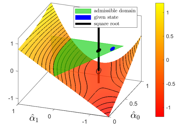
The fourth panel states the function $\nicefrac{{1}}{{3}}\;\hat{\alpha}^{\textup{T}}\mathcal{P}(\hat{\alpha})\hat{\alpha}-\hat{\alpha}^{\textup{T}}\widehat{\rho}$. It is convex on the green highlighted set, where the condition $\hat{\alpha}_{0}\geq|\hat{\alpha}_{1}|$ holds. For a fixed state $\widehat{\rho}=\widehat{\textup{{u}}}^{\ast 2}$ its minimum gives the desired gPC modes that are illustrated in the third panel. This also shows that the optimization problem is well-posed apart from states that are close to zero or result in too large random fluctuations. In those cases, assumption (2.12) is violated.

The optimization problem (2.10) allows to extend the Hamiltonian (1.3) to a stochastic Galerkin formulation. To this end, we assume an arbitrary, but consistent gPC approximation $\widehat{\textup{{v}}}(\textup{x})$ satisfying

$$\bigg\lVert v(\textup{x},\xi)-\sum\limits_{k=0}^{K}\widehat{\textup{{v}}}_{k}(\textup{x})\phi_{k}(\xi)\bigg\rVert_{\mathbb{P}}\rightarrow 0\quad\text{for}\quad K\rightarrow\infty.$$

The gPC formulation for the random Hamiltonian reads as

$$\widehat{\textup{{H}}}(\widehat{\textup{{u}}},\textup{x})\coloneqq\widehat{\textup{{v}}}(\textup{x})\ast\widehat{\,\lVert\textup{{u}}\rVert\,}.$$ (2.14)

The corresponding stochastic Galerkin formulations to the Hamilton-Jacobi equations (HJ) and the hyperbolic conservation laws (HC) are

$$\partial_{t}\widehat{\varphi}(t,\textup{x}) +\widehat{\textup{{H}}}\Big(\nabla_{\textup{x}}\widehat{\varphi}(t,\textup{x}),\textup{x}\Big) =0,$$ (HJ)

$$\partial_{t}\widehat{\textup{{u}}}(t,\textup{x}) +\nabla_{\textup{x}}\widehat{\textup{{H}}}\Big(\widehat{\textup{{u}}}(t,\textup{x}),\textup{x}\Big) =0,\quad\widehat{\textup{{u}}}(\textup{x})\coloneqq\nabla_{\textup{x}}\widehat{\varphi}(\textup{x}).$$ (HC)

In the case of deterministic initial data $\varphi_{0}(\textup{x})\in\mathbb{R}$ we have

$$\widehat{\varphi}_{k}(0,\textup{x})=\varphi_{0}(\textup{x})\delta_{k,0}\quad\text{and} \quad\widehat{\textup{{u}}}_{k}(0,\textup{x})=\nabla_{\textup{x}}\varphi_{0}(\textup{x})\delta_{k,0}.$$

In the sequel, the hyperbolic form (HC) with the Hamiltonian (2.14), which corresponds to the random level set equations, is analyzed in terms of hyperbolicity.

2.1 Eigenvalue decomposition and hyperbolicity

We distinguish between the following two formulations, which are formally equivalent provided that the matrix $\mathcal{P}\big(\widehat{\textup{{v}}}(\textup{x})\big)$ is invertible, but result in different theoretical and numerical solution concepts.

Conservative form

$\displaystyle\begin{aligned} &\partial_{t}\widehat{\textup{{u}}}(t,\textup{x})+\partial_{x_{1}}\widehat{f_{1}}\Big(\widehat{\textup{{u}}}(t,\textup{x}),\widehat{\textup{{v}}}(\textup{x})\Big)+\partial_{x_{2}}\widehat{f_{2}}\Big(\widehat{\textup{{u}}}(t,\textup{x}),\widehat{\textup{{v}}}(\textup{x})\Big)=0\\ &\text{with flux functions}\quad\widehat{f_{1}}\big(\widehat{\textup{{u}}},\widehat{\textup{{v}}}\big)=\begin{pmatrix}\widehat{\textup{{v}}}\ast\widehat{\,\lVert\textup{{u}}\rVert\,}\\ 0\end{pmatrix}\quad\text{and}\quad\widehat{f_{2}}\big(\widehat{\textup{{u}}},\widehat{\textup{{v}}}\big)=\begin{pmatrix}0\\ \widehat{\textup{{v}}}\ast\widehat{\,\lVert\textup{{u}}\rVert\,}\end{pmatrix}\end{aligned}$

Capacity form

$\displaystyle\begin{aligned} &\mathcal{P}\big(\widehat{\textup{{v}}}(\textup{x})\big)^{-1}\partial_{t}\widehat{\textup{{u}}}(t,\textup{x})+\partial_{x_{1}}\widetilde{f_{1}}\Big(\widehat{\textup{{u}}}(t,\textup{x})\Big)+\partial_{x_{2}}\widetilde{f_{2}}\Big(\widehat{\textup{{u}}}(t,\textup{x})\Big)\\ &\qquad\qquad=-\mathcal{P}\big(\widehat{\textup{{v}}}(\textup{x})\big)^{-1}\big(\partial_{x_{1}}+\partial_{x_{2}}\big)\widehat{\textup{{v}}}(\textup{x})\ \ast\widehat{\ \lVert\textup{{u}}(t,\textup{x})\rVert\ }\\ &\text{with flux functions}\quad\widetilde{f_{1}}\big(\widehat{\textup{{u}}}\big)=\begin{pmatrix}\widehat{\,\lVert\textup{{u}}\rVert\,}\\ 0\end{pmatrix}\quad\text{and}\quad\widetilde{f_{2}}\big(\widehat{\textup{{u}}}\big)=\begin{pmatrix}0\\ \widehat{\,\lVert\textup{{u}}\rVert\,}\end{pmatrix}\end{aligned}$

The following main theorem investigates the eigenvalue decomposition of both formulations. In particular the capacity form is proven strongly hyperbolic. The proof is inspired by the approach in [7, 8], where the Jacobian is shown to be similar to a symmetric matrix.

Theorem 2.1.

Let states $\widehat{\textup{{u}}}=\big(\widehat{\,\textup{{u}}_{1}},\widehat{\,\textup{{u}}_{2}}\big)^{\textup{T}}\in\mathbb{R}^{2(K+1)}$ and gPC modes ${\widehat{\textup{{v}}}}\in\mathbb{R}^{K+1}$ be given such that for all unit vectors $\vec{n}=(n_{1},n_{2})^{\textup{T}}$ the matrices $\widehat{\lambda}(\widehat{\textup{{u}}})\coloneqq n_{1}\mathcal{P}(\widehat{\,\textup{{u}}_{1}})+n_{2}\mathcal{P}(\widehat{\,\textup{{u}}_{2}})$, $\mathcal{P}\big(\widehat{\textup{{v}}}\big)$ are invertible and such that property (2.12) is satisfied. For all unit vectors $\vec{n}=(n_{1},n_{2})^{\textup{T}}$, the following statements hold:

1. The conservative form has the Jacobian
   

   $\displaystyle\begin{aligned} \widehat{\;\textup{{J}}}_{\vec{n}}(\widehat{\textup{{u}}},\widehat{\textup{{v}}})&\coloneqq n_{1}\textup{D}_{\widehat{\textup{{u}}}}\widehat{f_{1}}(\widehat{\textup{{u}}},\widehat{\textup{{v}}})+n_{2}\textup{D}_{\widehat{\textup{{u}}}}\widehat{f_{2}}(\widehat{\textup{{u}}},\widehat{\textup{{v}}})\\ &\;=\Big[\textup{diag}\{1,1\}\otimes\widehat{\,\mathcal{A}\;}(\widehat{\textup{{u}}},\widehat{\textup{{v}}})\Big]\begin{pmatrix}n_{1}\mathcal{P}\big(\widehat{\,\textup{{u}}_{1}}\big)&n_{1}\mathcal{P}\big(\widehat{\,\textup{{u}}_{2}}\big)\\ n_{2}\mathcal{P}\big(\widehat{\,\textup{{u}}_{1}}\big)&n_{2}\mathcal{P}\big(\widehat{\,\textup{{u}}_{2}}\big)\end{pmatrix}\end{aligned}$
   

   $\displaystyle\begin{aligned} &\text{which is similar to}&\widehat{\Lambda}(\widehat{\textup{{u}}},\widehat{\textup{{v}}})&\coloneqq\begin{pmatrix}\mathbb{O}&\mathbb{O}\\ \mathbb{O}&\widehat{\lambda}(\widehat{\textup{{u}}},\widehat{\textup{{v}}})\end{pmatrix}\\ &\text{with}\quad&\widehat{\lambda}(\widehat{\textup{{u}}},\widehat{\textup{{v}}})&\coloneqq\widehat{\,\mathcal{A}\;}(\widehat{\textup{{u}}},\widehat{\textup{{v}}})\Big[n_{1}\mathcal{P}(\widehat{\,\textup{{u}}_{1}})+n_{2}\mathcal{P}(\widehat{\,\textup{{u}}_{2}})\Big]\\ &\text{and}\quad&\widehat{\,\mathcal{A}\;}(\widehat{\textup{{u}}},\widehat{\textup{{v}}})&\coloneqq\mathcal{P}\big(\widehat{\textup{{v}}}\big)\mathcal{P}\Big(\widehat{\,\lVert\textup{{u}}\rVert\,}\Big)^{-1}.\end{aligned}$
   

2. The capacity form has the Jacobian
   

   $\displaystyle\begin{aligned} \widetilde{\;\textup{{J}}}_{\vec{n}}(\widehat{\textup{{u}}})&\coloneqq n_{1}\textup{D}_{\widehat{\textup{{u}}}}\widetilde{f_{1}}(\widehat{\textup{{u}}})+n_{2}\textup{D}_{\widehat{\textup{{u}}}}\widetilde{f_{2}}(\widehat{\textup{{u}}})\\ &\,=\bigg[\textup{diag}\{1,1\}\otimes\mathcal{P}\Big(\widehat{\,\lVert\textup{{u}}\rVert\,}\Big)^{-1}\bigg]\begin{pmatrix}n_{1}\mathcal{P}\big(\widehat{\,\textup{{u}}_{1}}\big)&n_{1}\mathcal{P}\big(\widehat{\,\textup{{u}}_{2}}\big)\\ n_{2}\mathcal{P}\big(\widehat{\,\textup{{u}}_{1}}\big)&n_{2}\mathcal{P}\big(\widehat{\,\textup{{u}}_{2}}\big)\end{pmatrix}\end{aligned}$
   

   and is similar to the symmetric matrix

   $$\widetilde{\Lambda}(\widehat{\textup{{u}}})\coloneqq\begin{pmatrix}\mathbb{O}&\mathbb{O}\\ \mathbb{O}&\widetilde{\lambda}(\widehat{\textup{{u}}})\end{pmatrix}\ \ \ \text{with}\ \ \ \widetilde{\lambda}(\widehat{\textup{{u}}})\coloneqq\mathcal{P}\Big(\widehat{\,\lVert\textup{{u}}\rVert\,}\Big)^{-\nicefrac{{1}}{{2}}}\Big[n_{1}\mathcal{P}(\widehat{\,\textup{{u}}_{1}})+n_{2}\mathcal{P}(\widehat{\,\textup{{u}}_{2}})\Big]\mathcal{P}\Big(\widehat{\,\lVert\textup{{u}}\rVert\,}\Big)^{-\nicefrac{{1}}{{2}}}.$$

Proof 2.2.

We introduce the injective mapping

$$\mathcal{T}\ \ :\ \ \mathbb{R}^{2(K+1)}\rightarrow\mathbb{R}^{K+1},\ \ \widehat{\textup{{u}}}\mapsto\widehat{\textup{{u}}}_{1}^{\ast 2}+\widehat{\textup{{u}}}_{2}^{\ast 2}$$

which has the Jacobian $\textup{D}_{\widehat{\,\textup{{u}}_{i}}}\mathcal{T}(\widehat{\textup{{u}}})=2\mathcal{P}(\widehat{\,\textup{{u}}_{i}})$ and we define $\mathcal{R}^{\prime}(\widehat{\textup{{u}}})\coloneqq\textup{D}_{\widehat{\textup{{u}}}}\mathcal{R}(\widehat{\textup{{u}}})=2\mathcal{P}\big(\widehat{\textup{{u}}}\big)$. Then, the Jacobian to the gPC modes (2.10) reads as

$$\textup{D}_{\widehat{\,\textup{{u}}_{i}}}\widehat{\,\lVert\textup{{u}}\rVert\,}=\textup{D}_{\widehat{\,\textup{{u}}_{i}}}\Big[\mathcal{R}^{-1}\big(\mathcal{T}(\widehat{\textup{{u}}})\big)\Big]=\bigg[\mathcal{R}^{\prime}\left(\widehat{\,\lVert\textup{{u}}\rVert\,}\right)\bigg]^{-1}\textup{D}_{\widehat{\,\textup{{u}}_{i}}}\mathcal{T}(\widehat{\textup{{u}}})=\mathcal{P}\Big(\widehat{\,\lVert\textup{{u}}\rVert\,}\Big)^{-1}\mathcal{P}\big(\widehat{\,\textup{{u}}_{i}}\big),$$

which yields the Jacobians $\widehat{\;\textup{{J}}}_{\vec{n}}(\widehat{\textup{{u}}},\widehat{\textup{{v}}})$ and $\widetilde{\;\textup{{J}}}_{\vec{n}}(\widehat{\textup{{u}}})$. Define the matrices

$$\widehat{\textbf{V}}(\widehat{\textup{{u}}},\widehat{\textup{{v}}}) \coloneqq\Big[\textup{diag}\{1,1\}\otimes\widehat{\lambda}(\widehat{\textup{{u}}},\widehat{\textup{{v}}}) \Big]^{-1} \begin{pmatrix}-\widehat{\,\mathcal{A}\;}(\widehat{\textup{{u}}},\widehat{\textup{{v}}})\mathcal{P}(\widehat{\,\textup{{u}}_{2}})\mathcal{P}(\widehat{\,\textup{{u}}_{1}})^{-1}\widehat{\,\mathcal{A}\;}(\widehat{\textup{{u}}},\widehat{\textup{{v}}})^{-1}&\frac{n_{1}}{n_{2}}\mathbbm{1}\\ \mathbbm{1}&\mathbbm{1}\end{pmatrix},$$

$$\widehat{\textbf{V}}(\widehat{\textup{{u}}},\widehat{\textup{{v}}})^{-1} \coloneqq\Big[\textup{diag}\{1,1\}\otimes\widehat{\,\mathcal{A}\;}(\widehat{\textup{{u}}},\widehat{\textup{{v}}}) \Big] \begin{pmatrix}-n_{2}\mathcal{P}(\widehat{\,\textup{{u}}_{1}})&n_{1}\mathcal{P}(\widehat{\,\textup{{u}}_{1}})\\ n_{2}\mathcal{P}(\widehat{\,\textup{{u}}_{1}})&n_{2}\mathcal{P}(\widehat{\,\textup{{u}}_{2}})\end{pmatrix},\quad\mathbbm{1}\coloneqq\textup{diag}\{1,\ldots,1\}.$$

Standard computations show

$$\widehat{\textbf{V}}(\widehat{\textup{{u}}},\widehat{\textup{{v}}})\widehat{\textbf{V}}(\widehat{\textup{{u}}},\widehat{\textup{{v}}})^{-1}=\mathbbm{1}\quad\text{and}\quad\widehat{\;\textup{{J}}}_{\vec{n}}(\widehat{\textup{{u}}},\widehat{\textup{{v}}})=\widehat{\textbf{V}}(\widehat{\textup{{u}}},\widehat{\textup{{v}}})\widehat{\Lambda}(\widehat{\textup{{u}}},\widehat{\textup{{v}}})\widehat{\textbf{V}}(\widehat{\textup{{u}}},\widehat{\textup{{v}}})^{-1},$$

which proves the first statement. The second statement follows analogously with the choice $\widehat{\textup{{v}}}=\widehat{\;e_{1}}$, i.e. $\mathcal{P}(\widehat{\textup{{v}}})=\mathbbm{1}$, and due to the matrix similarities

$$\widetilde{\;\textup{{J}}}_{\vec{n}}(\widehat{\textup{{u}}})=\widehat{\textbf{V}}(\widehat{\textup{{u}}},\widehat{\;e_{1}})\left(\textup{diag}\{1,1\}\otimes\Bigg[\mathcal{P}\Big(\widehat{\,\lVert\textup{{u}}\rVert\,}\Big)^{-\nicefrac{{1}}{{2}}}\ \,\widetilde{\lambda}(\widehat{\textup{{u}}})\ \mathcal{P}\Big(\widehat{\,\lVert\textup{{u}}\rVert\,}\Big)^{\nicefrac{{1}}{{2}}}\Bigg]\right)\widehat{\textbf{V}}(\widehat{\textup{{u}}},\widehat{\;e_{1}})^{-1}.$$

2.2 Relationship between the conservative and capacity form

We remark that the presented hyperbolicity results hold only local in time around states, where the assumptions of Theorem 2.1 are fulfilled, i.e. the matrix $\mathcal{P}\big(\widehat{\,\lVert\textup{{u}}\rVert\,}\big)$ is strictly positive definite. According to [32, Th. 2] and [17, Th. 2.1], this holds provided that realizations

$$\Pi_{K}\left[\widehat{\,\lVert\textup{{u}}\rVert\,}\right]\big(\xi(\omega)\big)=\sum\limits_{k=0}^{K}\left(\widehat{\,\lVert\textup{{u}}\rVert\,}\right)_{k}\phi_{K}\big(\xi(\omega)\big)>0$$ (2.15)

are almost surely strictly positive. Hence, there is a degeneracy of the Jacobian for a vanishing solution $\widehat{\textup{{u}}}\rightarrow(0,\ldots,0)^{\textup{T}}$. This is an expected property that is also observed in the deterministic case (1.7). Furthermore, Theorem 2.1 only guarantees that the Jacobian $\widetilde{\;\textup{{J}}}_{\vec{n}}(\widehat{\textup{{u}}})$ in the capacity form has real eigenvalues and a complete set of eigenvectors, since it is similar to a symmetric matrix. Hyperbolicity of the conservative form is not guaranteed, because the matrix $\widehat{\,\mathcal{A}\;}(\widehat{\textup{{u}}},\widehat{\textup{{v}}})$ is not necessarily symmetric and the square root may not exist. If the velocity is deterministic and positive, i.e. $v(\textup{x})>0$, we have $\widehat{\textup{{v}}}(\textup{x})=v(\textup{x})\widehat{\;e_{1}}$. Then, the matrix

$$\widehat{\,\mathcal{A}\;}(\widehat{\textup{{u}}},\widehat{\textup{{v}}})=v\,\mathcal{P}\Big(\widehat{\,\lVert\textup{{u}}\rVert\,}\Big)^{-1}$$

is symmetric and positive definite. In general however, the Jacobian $\widehat{\;\textup{{J}}}_{\vec{n}}(\widehat{\textup{{u}}},\widehat{\textup{{v}}})$ may have complex eigenvalues. An example is given in the appendix. Then, the capacity form has to be considered.

Note that this form naturally occurs e.g. in the derivation of conservation laws if the flux of a quantity is defined in terms of a quantity that is not conserved [23, Sec. 2.4, Sec. 6.16]. We consider an arbitrary spatial domain $C$, where the matrix $\mathcal{P}\big(\widehat{\textup{{v}}}(\textup{x})\big)$ is invertible. Then, the integral forms to the two-dimensional level set equations read as follows:

Conservative form

$\displaystyle\begin{aligned} \frac{\textup{d}}{\textup{d}t}\int_{C}\widehat{\textup{{u}}}(t,\textup{x})\,\textup{d}x=&-\int_{\partial C}n_{1}(s)\widehat{f_{1}}\Big(\widehat{\textup{{u}}}\big(t,\textup{x}(s)\big),\widehat{\textup{{v}}}\big(\textup{x}(s)\big)\Big)+n_{2}(s)\widehat{f_{2}}\Big(\widehat{\textup{{u}}}\big(t,\textup{x}(s)\big),\widehat{\textup{{v}}}\big(\textup{x}(s)\big)\Big)\,\textup{d}s\end{aligned}$

Capacity form

$\displaystyle\begin{aligned} \frac{\textup{d}}{\textup{d}t}\int_{C}\mathcal{P}\big(\widehat{\textup{{v}}}(\textup{x})\big)^{-1}\widehat{\textup{{u}}}(t,\textup{x})\,\textup{d}\textup{x}=&-\int_{\partial C}n_{1}(s)\widetilde{f_{1}}\Big(\widehat{\textup{{u}}}\big(t,\textup{x}(s)\big)\Big)+n_{2}(s)\widetilde{f_{2}}\Big(\widehat{\textup{{u}}}\big(t,\textup{x}(s)\big)\Big)\,\textup{d}s\\ &-\int_{C}\mathcal{P}\big(\widehat{\textup{{v}}}(\textup{x})\big)^{-1}\;\big(\partial_{x_{1}}+\partial_{x_{2}}\big)\widehat{\textup{{v}}}(\textup{x})\;\ast\widehat{\ \lVert\textup{{u}}(t,\textup{x})\rVert\ }\,\textup{d}\textup{x}.\end{aligned}$

3 Hyperbolicity preserving finite-volume discretization

To improve and faciliate the readability, we present the numerical discretization in one spatial dimension and we assume a constant velocity $\widehat{\textup{{v}}}(x)=\widehat{\textup{{v}}}$. Then, the conservative and capacity form read as

$$\partial_{t}\widehat{\textup{{u}}}(t,x)+\partial_{x}\widehat{f}\Big(\widehat{\textup{{u}}}(t,\textup{x}),\widehat{\textup{{v}}}\Big) =0\ \ \text{for}\ \ \widehat{f}\big(\widehat{\textup{{u}}},\widehat{\textup{{v}}}\big) =\widehat{\textup{{v}}}\ast\widehat{\,|\textup{{u}}|\,},\ \, \widehat{\;\textup{{J}}}\big(\widehat{\textup{{u}}},\widehat{\textup{{v}}}\big) =\mathcal{P}\big(\widehat{\textup{{v}}}\big)\widetilde{\;\textup{{J}}}\big(\widehat{\textup{{u}}}\big)$$

$$\mathcal{P}(\widehat{\textup{{v}}})^{-1} \partial_{t}\widehat{\textup{{u}}}(t,x)+\partial_{x}\widetilde{f}\Big(\widehat{\textup{{u}}}(t,\textup{x})\Big) =0\ \ \text{for}\ \ \widetilde{f}\big(\widehat{\textup{{u}}}\big) =\widehat{\,|\textup{{u}}|\,},\ \, \widetilde{\;\textup{{J}}}\big(\widehat{\textup{{u}}}\big) =\mathcal{P}\big(\widehat{\,|\textup{{u}}|\,}\big)^{-1}\mathcal{P}\big(\widehat{\textup{{u}}}\big),$$

where $\widehat{\;\textup{{J}}}\big(\widehat{\textup{{u}}},\widehat{\textup{{v}}}\big)\coloneqq\textup{D}_{\widehat{\textup{{u}}}}\widehat{f}\big(\widehat{\textup{{u}}},\widehat{\textup{{v}}}\big)$ and $\widetilde{\;\textup{{J}}}\big(\widehat{\textup{{u}}}\big)\coloneqq\textup{D}_{\widehat{\textup{{u}}}}\widetilde{f}\big(\widehat{\textup{{u}}}\big)$ denote the corresponding Jacobian. The interested reader finds the two-dimensional case with space-varying velocity in the appendix. The spatial domain is discretized in equidistant grid cells ${C_{j}\coloneqq\big(x_{j-\nicefrac{{1}}{{2}}},x_{j+\nicefrac{{1}}{{2}}}\big)\subset\mathbb{R}}$ with volume $\Delta x=x_{j+\nicefrac{{1}}{{2}}}-x_{j-\nicefrac{{1}}{{2}}}>0$ centered at $x_{j}$. The cell averages at time $t^{n}\in\mathbb{R}^{+}_{0}$ are denoted by $\hbox{\vbox{\hrule height=0.5pt\kern 2.15277pt\hbox{\kern-1.00006pt$\textup{{u}}$\kern-1.00006pt}}}_{j}^{n}$ and $\hbox{\vbox{\hrule height=0.5pt\kern 2.15277pt\hbox{\kern-1.00006pt$\textup{{w}}$\kern-1.00006pt}}}_{j}^{n}$.

3.1 Conservative form

Under the assumption of a real spectrum, which has been deduced in Theorem 2.1, the local Lax-Friedrichs flux reads as

$$\widehat{\mathcal{F}}\big(\hbox{\vbox{\hrule height=0.5pt\kern 2.15277pt\hbox{\kern-1.00006pt$\textup{{u}}$\kern-1.00006pt}}}_{\;\ell},\hbox{\vbox{\hrule height=0.5pt\kern 2.15277pt\hbox{\kern-1.00006pt$\textup{{u}}$\kern-1.00006pt}}}_{\;r},\widehat{\textup{{v}}}\big)\coloneqq\frac{1}{2}\Big(\widehat{f}\big(\hbox{\vbox{\hrule height=0.5pt\kern 2.15277pt\hbox{\kern-1.00006pt$\textup{{u}}$\kern-1.00006pt}}}_{\;\ell},\widehat{\textup{{v}}}\big)+\widehat{f}\big(\hbox{\vbox{\hrule height=0.5pt\kern 2.15277pt\hbox{\kern-1.00006pt$\textup{{u}}$\kern-1.00006pt}}}_{\;r},\widehat{\textup{{v}}}\big)\Big)-\frac{1}{2}\max\limits_{q=\ell,r}\Big\{\sigma\Big\{\widehat{\;\textup{{J}}}\big(\hbox{\vbox{\hrule height=0.5pt\kern 2.15277pt\hbox{\kern-1.00006pt$\textup{{u}}$\kern-1.00006pt}}}_{\;q},\widehat{\textup{{v}}}\big)\Big\}\Big\}\big(\hbox{\vbox{\hrule height=0.5pt\kern 2.15277pt\hbox{\kern-1.00006pt$\textup{{u}}$\kern-1.00006pt}}}_{\;r}-\hbox{\vbox{\hrule height=0.5pt\kern 2.15277pt\hbox{\kern-1.00006pt$\textup{{u}}$\kern-1.00006pt}}}_{\;\ell}\big),$$ (3.16)

where ${\sigma\{\cdot\}}$ denotes the spectral radius. Then, a first-order finite-volume discretization reads as

$$\hbox{\vbox{\hrule height=0.5pt\kern 2.15277pt\hbox{\kern-1.00006pt$\textup{{u}}$\kern-1.00006pt}}}_{j}^{n+1}=\hbox{\vbox{\hrule height=0.5pt\kern 2.15277pt\hbox{\kern-1.00006pt$\textup{{u}}$\kern-1.00006pt}}}_{j}^{n}-\frac{\Delta t}{\Delta x}\bigg[\widehat{\mathcal{F}}\left(\hbox{\vbox{\hrule height=0.5pt\kern 2.15277pt\hbox{\kern-1.00006pt$\textup{{u}}$\kern-1.00006pt}}}_{j}^{n},\hbox{\vbox{\hrule height=0.5pt\kern 2.15277pt\hbox{\kern-1.00006pt$\textup{{u}}$\kern-1.00006pt}}}_{j+1}^{n},\widehat{\textup{{v}}}\right)-\widehat{\mathcal{F}}\left(\hbox{\vbox{\hrule height=0.5pt\kern 2.15277pt\hbox{\kern-1.00006pt$\textup{{u}}$\kern-1.00006pt}}}_{j-1}^{n},\hbox{\vbox{\hrule height=0.5pt\kern 2.15277pt\hbox{\kern-1.00006pt$\textup{{u}}$\kern-1.00006pt}}}_{j}^{n},\widehat{\textup{{v}}}\right)\bigg].$$ (3.17)

Provided that the CFL-condition

$$\max\limits_{j\in\mathbb{N}}\Big\{\sigma\left\{\widehat{\;\textup{{J}}}\big(\hbox{\vbox{\hrule height=0.5pt\kern 2.15277pt\hbox{\kern-1.00006pt$\textup{{u}}$\kern-1.00006pt}}}_{j}^{n},\widehat{\textup{{v}}}\big)\right\}\Big\}\frac{\Delta t}{\Delta x}<1$$ (3.18)

holds, the discrete solution converges to the weak entropy solution [23].

3.2 Capacity form

We have already remarked that the conservative form is hyperbolic if the velocity is deterministic. Then, the CFL-condition ensures that the dependency of the true solution is within the numerical range [23, Sec. 4.4], which results in a convergent numerical scheme. Applying the stochastic Galerkin method to random velocities, however, results in additional waves that influence the numerical dependence on the solution. The idea of the hyperbolicity preserving discretization is to introduce a non-uniform effective grid to capture the numerical dependence in an appropriate way. Using the orthogonal eigenvalue decomposition $\mathcal{P}(\widehat{\textup{{v}}})=\mathcal{V}(\widehat{\textup{{v}}})\mathcal{D}(\widehat{\textup{{v}}})\mathcal{V}(\widehat{\textup{{v}}})^{\textup{T}},$ the one-dimensional capacity form is equivalent to

$$\mathcal{D}(\widehat{\textup{{v}}})^{-1}\partial_{t}\widehat{\textup{{w}}}(t,x)+\partial_{x}\widetilde{F}^{(\textup{eff})}\big(\widehat{\textup{{w}}}(t,x),\widehat{\textup{{v}}}\big)=0\quad\text{with}$$ (3.19)

$$\widehat{\textup{{w}}}\coloneqq\mathcal{V}(\widehat{\textup{{v}}})^{\textup{T}}\widehat{\textup{{u}}}\quad\text{and}\quad\widetilde{F}^{(\textup{eff})}\big(\widehat{\textup{{w}}},\widehat{\textup{{v}}}\big)\coloneqq\mathcal{V}(\widehat{\textup{{v}}})^{\textup{T}}\,\widetilde{f}\big(\mathcal{V}(\widehat{\textup{{v}}})\widehat{\textup{{w}}}\big).$$

The $k$-th component of the vector valued cell average $\hbox{\vbox{\hrule height=0.5pt\kern 2.15277pt\hbox{\kern-1.00006pt$\textup{{w}}$\kern-1.00006pt}}}_{j}^{n}\in\mathbb{R}^{K+1}$ is given by the recursion

$$\left(\hbox{\vbox{\hrule height=0.5pt\kern 2.15277pt\hbox{\kern-1.00006pt$\textup{{w}}$\kern-1.00006pt}}}_{j}^{n+1}\right)_{k}=\left(\hbox{\vbox{\hrule height=0.5pt\kern 2.15277pt\hbox{\kern-1.00006pt$\textup{{w}}$\kern-1.00006pt}}}_{j}^{n}\right)_{k}-\frac{{\Delta t}}{\Delta\tilde{v}_{k}}\bigg[\widetilde{\mathcal{F}}_{k}^{(\textup{gLF})}\left(\hbox{\vbox{\hrule height=0.5pt\kern 2.15277pt\hbox{\kern-1.00006pt$\textup{{w}}$\kern-1.00006pt}}}_{j}^{n},\hbox{\vbox{\hrule height=0.5pt\kern 2.15277pt\hbox{\kern-1.00006pt$\textup{{w}}$\kern-1.00006pt}}}_{j+1}^{n},\widehat{\textup{{v}}}\right)-\widetilde{\mathcal{F}}_{k}^{(\textup{gLF})}\left(\hbox{\vbox{\hrule height=0.5pt\kern 2.15277pt\hbox{\kern-1.00006pt$\textup{{w}}$\kern-1.00006pt}}}_{j-1}^{n},\hbox{\vbox{\hrule height=0.5pt\kern 2.15277pt\hbox{\kern-1.00006pt$\textup{{w}}$\kern-1.00006pt}}}_{j}^{n},\widehat{\textup{{v}}}\right)\bigg]$$ (3.20)

$$\text{with the effective volume}\quad\Delta\tilde{v}_{k}\coloneqq\frac{\Delta x}{\mathcal{D}_{k}(\widehat{\textup{{v}}})}.$$

Here, the componentwise global Lax-Friedrichs flux takes the effective volume into account and reads as

$$\widetilde{\mathcal{F}}_{k}^{(\textup{gLF})}\big(\hbox{\vbox{\hrule height=0.5pt\kern 2.15277pt\hbox{\kern-1.00006pt$\textup{{w}}$\kern-1.00006pt}}}_{\;\ell},\hbox{\vbox{\hrule height=0.5pt\kern 2.15277pt\hbox{\kern-1.00006pt$\textup{{w}}$\kern-1.00006pt}}}_{\;r},\widehat{\textup{{v}}}\big)\coloneqq\frac{1}{2}\Big(\widetilde{F}^{(\textup{eff})}_{k}\big(\hbox{\vbox{\hrule height=0.5pt\kern 2.15277pt\hbox{\kern-1.00006pt$\textup{{w}}$\kern-1.00006pt}}}_{\;\ell},\widehat{\textup{{v}}}\big)+\widetilde{F}^{(\textup{eff})}_{k}\big(\hbox{\vbox{\hrule height=0.5pt\kern 2.15277pt\hbox{\kern-1.00006pt$\textup{{w}}$\kern-1.00006pt}}}_{\;r},\widehat{\textup{{v}}}\big)\Big)-\frac{1}{2}\frac{\Delta\tilde{v}_{k}}{\Delta t}\big(\hbox{\vbox{\hrule height=0.5pt\kern 2.15277pt\hbox{\kern-1.00006pt$\textup{{w}}$\kern-1.00006pt}}}_{\;r}-\hbox{\vbox{\hrule height=0.5pt\kern 2.15277pt\hbox{\kern-1.00006pt$\textup{{w}}$\kern-1.00006pt}}}_{\;\ell}\big).$$ (3.21)

We observe from the diffusion part of the componentwise numerical flux function (3.21) that the resulting CFL-condition is

$$\textbf{v}_{\max}\ \max\limits_{j\in\mathbb{N}}\Big\{\sigma\left\{\widetilde{\;\textup{{J}}}\big(\hbox{\vbox{\hrule height=0.5pt\kern 2.15277pt\hbox{\kern-1.00006pt$\textup{{u}}$\kern-1.00006pt}}}_{j}^{n}\big)\right\}\Big\}\frac{\Delta t}{\Delta x}<1\quad\text{for}\quad\textbf{v}_{\max}\coloneqq\max\limits_{k=0,\ldots,K}\Big\{\big|\mathcal{D}_{k}(\widehat{\textup{{v}}})\big|\Big\}\quad\text{and}\quad\hbox{\vbox{\hrule height=0.5pt\kern 2.15277pt\hbox{\kern-1.00006pt$\textup{{u}}$\kern-1.00006pt}}}_{j}^{n}=\mathcal{V}(\widehat{\textup{{v}}})\hbox{\vbox{\hrule height=0.5pt\kern 2.15277pt\hbox{\kern-1.00006pt$\textup{{w}}$\kern-1.00006pt}}}_{j}^{n}.$$

Following [23, Sec. 6.17], we view the scheme (3.20) as a non-uniform effective space discretizations $\Delta\tilde{v}_{k}\in\mathbb{R}$ that is related by a coordinate transform to a uniform computational domain $\Delta x\in\mathbb{R}^{+}$. At this point, we emphasize that we do not make any assumption on the direction of the random velocities and hence on the sign of the effective volume. This is a desired result, since the solution to the level set equations behaves symmetric in terms of the sign of the velocity. We introduce for each component $\widehat{\textup{{w}}}_{k}$ the change of variables $\varphi_{k}(x)=\tilde{v}$ satisfying $\varphi_{k}^{\prime}(x)\mathcal{D}_{k}\big(\widehat{\textup{{v}}}(x)\big)=1$ and $\widehat{\textup{{w}}}_{k}(t,x)=\widetilde{\textit{{w}}}_{k}\big(t,\varphi_{k}(x)\big)$. This yields

$$\int_{x_{j-\nicefrac{{1}}{{2}}}}^{x_{j+\nicefrac{{1}}{{2}}}}\widehat{\textup{{w}}}_{k}\big(t,x\big)\mathcal{D}_{k}\big(\widehat{\textup{{v}}}(x)\big)^{-1}\,\textup{d}x=\int_{x_{j-\nicefrac{{1}}{{2}}}}^{x_{j+\nicefrac{{1}}{{2}}}}\widetilde{\textit{{w}}}_{k}\big(t,\varphi_{k}(x)\big)\varphi_{k}^{\prime}(x)\,\textup{d}x=\int_{\tilde{v}_{j-\nicefrac{{1}}{{2}},k}}^{\tilde{v}_{j+\nicefrac{{1}}{{2}},k}}\widetilde{\textit{{w}}}_{k}\big(t,\tilde{v}\big)\,\textup{d}\tilde{v}$$

for $\tilde{v}_{j\pm\nicefrac{{1}}{{2}},k}\coloneqq\varphi_{k}(x_{j\pm\nicefrac{{1}}{{2}},k})$. Therefore, the capacity form

$$\frac{\textup{d}}{\,\textup{d}t}\int_{x_{j-\nicefrac{{1}}{{2}}}}^{x_{j+\nicefrac{{1}}{{2}}}}\widehat{\textup{{w}}}_{k}\big(t,x\big)\mathcal{D}_{k}\big(\widehat{\textup{{v}}}(x)\big)^{-1}\,\textup{d}x=\widetilde{F}^{(\textup{eff})}_{k}\Big(\widehat{\textup{{w}}}\big(t,x_{j-\nicefrac{{1}}{{2}}}\big),\widehat{\textup{{v}}}\Big)-\widetilde{F}^{(\textup{eff})}_{k}\Big(\widehat{\textup{{w}}}\big(t,x_{j+\nicefrac{{1}}{{2}}}\big),\widehat{\textup{{v}}}\Big)$$

on the computational domain can be rewritten into the conservative form

$$\frac{\textup{d}}{\,\textup{d}t}\int_{\tilde{v}_{j-\nicefrac{{1}}{{2}},k}}^{\tilde{v}_{j+\nicefrac{{1}}{{2}},k}}\widetilde{\textit{{w}}}_{k}\big(t,\tilde{v}\big)\,\textup{d}\tilde{v}=\widetilde{F}^{(\textup{eff})}_{k}\Big(\widetilde{\textit{{w}}}\big(t,\tilde{v}_{j-\nicefrac{{1}}{{2}},k}\big),\widehat{\textup{{v}}}\Big)-\widetilde{F}^{(\textup{eff})}_{k}\Big(\widetilde{\textit{{w}}}\big(t,\tilde{v}_{j+\nicefrac{{1}}{{2}},k}\big),\widehat{\textup{{v}}}\Big).$$ (3.22)

Figure 2 illustrates the previous analysis. The left panel shows the uniform computational domain in black. The propagation of the continuous solution is exemplified by a blue and red, dashed arrow. The case when the true solution (red arrow) is not within the numerical range may happen for the conservative form if the Jacobian $\widehat{\;\textup{{J}}}\big(\widehat{\textup{{u}}},\widehat{\textup{{v}}}\big)$ has complex eigenvalues. In contrast, the capacity-form differencing scheme leads to a stable discretization as illustrated by the blue arrow. The right panel shows the case when the $k$-th component has a fast speed $\mathcal{D}_{k}\big(\widehat{\textup{{v}}}(x)\big)$, which results in a faster propagation of the true solution (blue arrow). This requires a larger effective volume $\Delta\tilde{v}_{j,k}=\tilde{v}_{j+\nicefrac{{1}}{{2}},k}-\tilde{v}_{j-\nicefrac{{1}}{{2}},k}$. Furthermore, the effective volume satisfies the conservative form (3.22).

Figure 2: Uniform computational domain (left): Blue arrow illustrates the capacity-form differencing scheme, red arrow a wrong estimation of characteristic speeds. Non-uniform effective volume (right): Green area shows the conserved quantity (3.22), the blue arrow exemplifies a solution that is propagated with a faster (random) speed, which needs a larger effective volume $\Delta\tilde{v}_{j,k}$.

Finally, we remark that the hyperbolicity preserving scheme (3.20) can be implemented in a similar way as the conservative update (3.17). Furthermore, the assumption $\mathcal{D}_{k}\big(\widehat{\textup{{v}}}(x)\big)\neq 0$ is not required if the update is defined as

$$\hbox{\vbox{\hrule height=0.5pt\kern 2.15277pt\hbox{\kern-1.00006pt$\textup{{w}}$\kern-1.00006pt}}}_{j}^{n+1} \;=\,\hbox{\vbox{\hrule height=0.5pt\kern 2.15277pt\hbox{\kern-1.00006pt$\textup{{w}}$\kern-1.00006pt}}}_{j}^{n}-\frac{{\Delta t}}{\Delta x}\bigg[\widetilde{\mathcal{F}}\left(\hbox{\vbox{\hrule height=0.5pt\kern 2.15277pt\hbox{\kern-1.00006pt$\textup{{w}}$\kern-1.00006pt}}}_{j}^{n},\hbox{\vbox{\hrule height=0.5pt\kern 2.15277pt\hbox{\kern-1.00006pt$\textup{{w}}$\kern-1.00006pt}}}_{j+1}^{n},\widehat{\textup{{v}}}\right)-\widetilde{\mathcal{F}}\left(\hbox{\vbox{\hrule height=0.5pt\kern 2.15277pt\hbox{\kern-1.00006pt$\textup{{w}}$\kern-1.00006pt}}}_{j-1}^{n},\hbox{\vbox{\hrule height=0.5pt\kern 2.15277pt\hbox{\kern-1.00006pt$\textup{{w}}$\kern-1.00006pt}}}_{j}^{n},\widehat{\textup{{v}}}\right)\bigg],$$

$$\widetilde{\mathcal{F}}\big(\hbox{\vbox{\hrule height=0.5pt\kern 2.15277pt\hbox{\kern-1.00006pt$\textup{{w}}$\kern-1.00006pt}}}_{\;\ell},\hbox{\vbox{\hrule height=0.5pt\kern 2.15277pt\hbox{\kern-1.00006pt$\textup{{w}}$\kern-1.00006pt}}}_{\;r},\widehat{\textup{{v}}}\big) \coloneqq\frac{1}{2}\Big(\widetilde{F}\big(\hbox{\vbox{\hrule height=0.5pt\kern 2.15277pt\hbox{\kern-1.00006pt$\textup{{w}}$\kern-1.00006pt}}}_{\;\ell},\widehat{\textup{{v}}}\big)+\widetilde{F}\big(\hbox{\vbox{\hrule height=0.5pt\kern 2.15277pt\hbox{\kern-1.00006pt$\textup{{w}}$\kern-1.00006pt}}}_{\;r},\widehat{\textup{{v}}}\big)\Big)-\frac{1}{2}\max\limits_{q=\ell,r}\Big\{\sigma\Big\{\widetilde{\;\textup{{J}}}\big(\hbox{\vbox{\hrule height=0.5pt\kern 2.15277pt\hbox{\kern-1.00006pt$\textup{{w}}$\kern-1.00006pt}}}_{\;q})\Big\}\Big\}\big(\hbox{\vbox{\hrule height=0.5pt\kern 2.15277pt\hbox{\kern-1.00006pt$\textup{{w}}$\kern-1.00006pt}}}_{\;r}-\hbox{\vbox{\hrule height=0.5pt\kern 2.15277pt\hbox{\kern-1.00006pt$\textup{{w}}$\kern-1.00006pt}}}_{\;\ell}\big),$$

$$\widetilde{F}\big(\hbox{\vbox{\hrule height=0.5pt\kern 2.15277pt\hbox{\kern-1.00006pt$\textup{{w}}$\kern-1.00006pt}}},\widehat{\textup{{v}}}\big) \coloneqq\mathcal{D}\big(\widehat{\textup{{v}}}(x)\big)\mathcal{V}(\widehat{\textup{{v}}})^{\textup{T}}\,\widetilde{f}\big(\mathcal{V}(\widehat{\textup{{v}}})\hbox{\vbox{\hrule height=0.5pt\kern 2.15277pt\hbox{\kern-1.00006pt$\textup{{w}}$\kern-1.00006pt}}}\big).$$

3.3 Computing the quantile of the perturbed level set

For convenience of the reader we follow the elementary argument in [19, Sec. 2] that shows how the desired solution $\widehat{\varphi}$ is obtained by the hyperbolic form (HC) with solution $\widehat{\textup{{u}}}=\nabla_{\textup{x}}\hat{\varphi}$, considered in Theorem 2.1 and Section 3 in terms of a zero viscosity limit. To this end, we assume $\widehat{\textup{{u}}}\in L^{\infty}\big((0,T)\times\mathbb{R}^{d};\mathbb{R}^{d(K+1)}\big)$ is a weak viscosity solution to the hyperbolic form (HC). Then, there exists a smooth solution $\widehat{\textup{{u}}}^{\varepsilon}\in C^{2}\big((0,T)\times\mathbb{R}^{d};\mathbb{R}^{d(K+1)}\big)$ to the viscous Cauchy problem

$$\partial_{t}\widehat{\textup{{u}}}^{\varepsilon}(t,\textup{x})+\nabla_{\textup{x}}\widehat{\textup{{H}}}\Big(\widehat{\textup{{u}}}^{\varepsilon}(t,\textup{x}),\textup{x}\Big)=\varepsilon\Delta_{\textup{x}}\widehat{\textup{{u}}}^{\varepsilon}(t,\textup{x})\quad\text{for}\quad\widehat{\textup{{u}}}^{\varepsilon}(0,\textup{x})=\mathcal{I}_{\widehat{\textup{{u}}}}(\textup{x}),$$ (3.23)

where we assume for simplicity smooth initial data. Furthermore, there exists a constant $c>0$ such that for any $m<\infty$ we have

$$\big\lVert\widehat{\textup{{u}}}^{\varepsilon}\big\rVert_{L^{\infty}}<c\quad\text{for all}\quad\varepsilon>0\quad\text{and}\quad\widehat{\textup{{u}}}^{\varepsilon}\overset{L^{\infty}}{\rightharpoonup}\widehat{\textup{{u}}}\in L^{m}\quad\text{in the limit}\quad\varepsilon\rightarrow 0.$$ (3.24)

We consider the heat equations

$$\partial_{t}\widehat{\varphi}^{\varepsilon}(t,\textup{x}) -\varepsilon\Delta_{\textup{x}}\widehat{\varphi}^{\varepsilon}(t,\textup{x}) =- \widehat{\textup{{H}}}\Big(\widehat{\textup{{u}}}^{\varepsilon}(t,\textup{x}),\textup{x}\Big) \quad\text{for}\quad\widehat{\varphi}^{\varepsilon}(0,\textup{x}) = \mathcal{I}_{\widehat{\varphi}}(\textup{x}),$$ (3.25)

$$\partial_{t}\widehat{\varphi}_{\textup{x}}^{\varepsilon}(t,\textup{x}) -\varepsilon\Delta_{\textup{x}}\widehat{\varphi}_{\textup{x}}^{\varepsilon}(t,\textup{x}) =-\nabla_{\textup{x}} \widehat{\textup{{H}}}\Big(\widehat{\textup{{u}}}^{\varepsilon}(t,\textup{x}),\textup{x}\Big) \quad\text{for}\quad\widehat{\varphi}_{\textup{x}}^{\varepsilon}(0,\textup{x}) =\nabla_{\textup{x}} \mathcal{I}_{\widehat{\varphi}}(\textup{x}),$$ (3.26)

where the states $\widehat{\varphi}_{\textup{x}}\coloneqq\nabla_{\textup{x}}\widehat{\varphi}$ are obtained by differentiating equation (3.25). Since equation (3.25) is a system of decoupled heat equations, a maximum principle can be applied to each component. Hence, there exist constants $C_{{k}}(T)>0$ such that the bound $\big|\widehat{\varphi}_{{k}}\big|\leq C_{k}(T)$ holds for all $t\in(0,T]$, which are independent for $\varepsilon>0$ due to property (3.24). Subtracting the viscous form (3.23) from the heat equation (3.26) yields

$$\partial_{t}\Big(\widehat{\varphi}_{\textup{x}}^{\varepsilon}-\widehat{\textup{{u}}}^{\varepsilon}\Big)(t,\textup{x})-\varepsilon\Delta_{\textup{x}}\Big(\widehat{\varphi}_{\textup{x}}^{\varepsilon}-\widehat{\textup{{u}}}^{\varepsilon}\Big)(t,\textup{x})=0\quad\text{for}\quad\Big(\widehat{\varphi}_{\textup{x}}^{\varepsilon}-\widehat{\textup{{u}}}^{\varepsilon}\Big)(0,\textup{x})=0.$$

The uniqueness of this Cauchy problem yields the relation $\widehat{\varphi}_{\textup{x}}^{\varepsilon}(t,\textup{x})=\widehat{\textup{{u}}}^{\varepsilon}(t,\textup{x})$ and equation (3.25) reads as

$$\partial_{t}\widehat{\varphi}^{\varepsilon}(t,\textup{x})+\widehat{\textup{{H}}}\Big(\nabla_{\textup{x}}\widehat{\varphi}^{\varepsilon}(t,\textup{x}),\textup{x}\Big)=\varepsilon\Delta_{\textup{x}}\widehat{\varphi}^{\varepsilon}(t,\textup{x}).$$

Since $\widehat{\varphi}^{\varepsilon}$ is uniformly bounded in $W^{1,\infty}$, there exists a unique viscosity solution $\widehat{\varphi}\in W^{1,\infty}$ that satisfies $\nabla_{\textup{x}}\widehat{\varphi}=\widehat{\textup{{u}}}$ almost everywhere.

Remark 3.1.

We refer the interested reader to [19, 21, 6] for more details on the relation in terms of viscosity solutions. The converse statement in the deterministic case, i.e. u is the vanishing viscosity solution if $\varphi$ is a viscosity solution, can be shown by exploiting the convexity of the deterministic Hamiltonian.

The projected Hamiltonian $\widehat{\textup{{H}}}$, however, is not a scalar function. Therefore, the converse statement is not straightforward and left here as an open problem. In this work the analysis is carried out in the variable $\widehat{\textup{{u}}}$. Hence, it is only relevant that $\widehat{\varphi}$ is a viscosity solution for given $\widehat{\textup{{u}}}$.

Finally, we note that the matrices $\mathcal{M}_{k}$ in the definition (2.9) can be exactly precomputed by Gaussian quadrature. According to [15, Sec. 5.1], the positive definiteness assumption (2.12), which is required for the optimization problem (2.10), may be efficiently verified by evaluating condition (2.15) at quadrature nodes $\xi^{(1)},\ldots,\xi^{(Q)}$. Namely, the inequalities

$$\Pi_{K}\left[\widehat{\,\lVert\textup{{u}}\rVert\,}\right]\left(\xi^{(q)}\right)>0\quad\text{must hold at all nodes}\quad\xi^{(1)},\ldots,\xi^{(Q)}.$$ (3.27)

4 Computational experiments

The theoretical results are illustrated numerically for a Riemann problem with deterministic initial values

$$\textup{{u}}(0,x)=\begin{cases}-1&\text{for}\ \ x<0,\\ \hphantom{+}1&\text{for}\ \ x>0\end{cases}\quad\text{and uniformly distributed velocity}\quad v(\xi)\sim\mathcal{U}\big(\nicefrac{{1}}{{2}},\nicefrac{{3}}{{2}}\big).$$

The exact solution reads as

$$\textup{{u}}(t,x,\xi)=\begin{cases}-1&\text{for}\ \ x<tv(\xi),\\ \hphantom{+}1&\text{for}\ \ x>tv(\xi)\end{cases}\quad\text{and}\quad\textup{{u}}(t,x,\xi)=0\quad\text{otherwise}.$$ (4.28)

As remarked in Section 2.2, the presented stochastic Galerkin formulations are only obtained by a well-posed optimization problem provided that assumption (2.12) holds, which is computationally verified by the inequality (2.15). In the other case, regularization techniques are needed. More precisely, we consider a treshold parameter $0<\textup{T}\ll 1$ and define the set

$$\mathbb{T}\coloneqq\bigg\{x\in\mathbb{R}\ \Big|\ \Pi_{K}\left[\widehat{\,\lVert\textup{{u}}\rVert\,}\right](\xi)<\textup{T}\bigg\},$$

where the optimization problem (2.10) is not necessarily well-posed. In this set we use the gPC expansion with two modes, i.e. the truncation $K=1$. Then, the gPC modes of the norm and the Jacobian are explicitly obtained by the equality (2.13) and read as

$$\widehat{\,\lVert\textup{{u}}\rVert\,}=\frac{1}{2}\begin{pmatrix}\big|\widehat{\textup{{u}}}_{0}+\widehat{\textup{{u}}}_{1}\big|+\big|\widehat{\textup{{u}}}_{0}-\widehat{\textup{{u}}}_{1}\big|\\ \big|\widehat{\textup{{u}}}_{0}+\widehat{\textup{{u}}}_{1}\big|-\big|\widehat{\textup{{u}}}_{0}-\widehat{\textup{{u}}}_{1}\big|\end{pmatrix}\quad\text{with}\quad\widetilde{\;\textup{{J}}}\big(\widehat{\textup{{u}}}\big)=\textup{D}_{\widehat{\textup{{u}}}}\widehat{\,\lVert\textup{{u}}\rVert\,}=\begin{pmatrix}s_{1}(\widehat{\textup{{u}}})&s_{2}(\widehat{\textup{{u}}})\\ s_{2}(\widehat{\textup{{u}}})&s_{1}(\widehat{\textup{{u}}})\end{pmatrix},$$

$$\text{for}\ \ s_{1}(\widehat{\textup{{u}}})\coloneqq\textup{sign}\big(\widehat{\textup{{u}}}_{0}+\widehat{\textup{{u}}}_{1}\big)+\textup{sign}\big(\widehat{\textup{{u}}}_{0}-\widehat{\textup{{u}}}_{1}\big)\ \ \text{and}\ \ s_{2}(\widehat{\textup{{u}}})\coloneqq\textup{sign}\big(\widehat{\textup{{u}}}_{0}+\widehat{\textup{{u}}}_{1}\big)-\textup{sign}\big(\widehat{\textup{{u}}}_{0}-\widehat{\textup{{u}}}_{1}\big).$$

Likewise to the deterministic case (1.7), the derivative of the norm is understood as the generalized gradient [4, 13, 5]. It is important to note that the reduction of the gPC truncation to $K=1$ decreases the spectrum that enters the local Lax-Friedrichs flux. Hence, this approach does not ensure enough numerical viscosity for a stable finite-volume discretization. To this end, the local Lax-Friedrichs flux is replaced by the global flux, however, only for states that belong to the domain $\mathbb{T}$. In the other case, the numerical discretizations of Section 3 are used. Finally, we emphasize that the conservative form is only included for comparison, since hyperbolicity is not necessarily guaranteed as the counterexample in Appendix A shows.

capacity form

spatial domain

conservative form

spatial domain

Figure 3: Numerical results for the conservative form presented in Section 3.1 and capacity form in Section 3.2. The spatial discretization is $\Delta x=2^{-6}$, the final time is $t=1$ and the CFL number is chosen as $\textup{CFL}=0.95$. The solid red line states the mean of the reference solution and the numerical solutions to the stochastic Galerkin systems are blue dotted. The zoom in the upper left corner highlights the domain close to the random level-set where oscillations occur due to the ill-posed optimization problem (2.10). The zoom in the lower right corner shows a region where the assumptions in Theorem 2.1 hold.

Computational results are given in Figure 3 for the capacity form (left panel) and conservative form (right panel). Therein, the reference solution (4.28) at time $t=1$ is stated in terms of the mean, which is plotted as red solid line. The mean of the stochastic Galerkin formulation with truncation $K=6$, i.e. the gPC mode $\widehat{\textup{{u}}}_{0}(1,x)$, is the blue dotted line.

The numerical experiments, which are shown in the left panel for the capacity form, indicate that the capacity-form differencing scheme leads to minior computational errors apart from the random level-set. In regions where the optimization problem is not necessarily well-posed, however, significant errors occur. This shows the need for regularization techniques, as e.g. used in [1], or piecewise ansatz functions that exploit the local structures in contrast to globally defined Legendre polynomials.

Since the uncertainty arisis in this problem from the velocity, the conservative form can be non-hyperbolic. Hence, the numerical solution of a finite-volume method, which is shown in the right panel, differs significantly from the reference solution. This explains the need for considering a numerical discretization of the capacity form.

5 Summary and outlook

We have analyzed the mathematical description of random zero-level sets that describe moving interfaces. The underlying equations are in Hamilton-Jacobi form, but are equivalent to a hyperbolic form in the sense of viscosity solutions, which have been analyzed in terms of hyperbolicity.

Figure 4 summarizes the theoretical results. It distinguishes between the red area (left), which corresponds to solutions satisfying $\Pi_{K}\big[\widehat{\,\lVert\textup{{u}}\rVert\,}\big]\big(\xi(\omega)\big)>0$, and the random interface (right, blue), where realizations may be non-positive. In the left, red region the optimization problem (2.10) is well-posed and Theorem 2.1 ensures hyperbolicity for all basis functions. For solutions that are closer to the zero-level set, the optimization problem (2.10) may have a solution that results in non-positive realizations $\Pi_{K}\big[\widehat{\,\lVert\textup{{u}}\rVert\,}\big]\big(\xi(\omega)\big)\leq 0$. Then, the matrix (2.12) may be indefinite [17, Th. 2.1]. These, negative realizations may result from projection errors, when the Galerkin method is used for higher polynomial ansatz functions. Since the presented intrusive approach allows to precompute all stochastic quantities exactly, an efficient criterium (3.27) that verifies the assumptions of Theorem 2.1 is to test positivity of the truncated polynomial chaos expansions at the quadrature nodes.

The case, when states are close to the boundary of the random interface, where the minimization problem (2.10) is ill-posed, involves additional theoretical and numerical challenges. It is an active field of research to introduce regularization techniques [1] and piecewise ansatz function, as e.g. wavelet basis, that exploit the local structures.

Figure 4: Illustration of the theoretical results: The left, red area includes states that satisfy the assumptions of Theorem 2.1 for all basis functions. A perturbed level set (1.8) is green, dashed exemplified. The right, blue domain illustrates the zero-level set. The random interface is a region, where expansions may result in both positive and vanishing realizations such that assumption (2.12) is violated.

Appendix

For the sake of completeness we state an example when the presented conservative form loses its hyperbolic character. Furthermore, the numerical discretizations in Section 3 are extended to space-varying velocities and two dimensions.

Appendix A Loss of hyperbolicity

To give an example such that the Jacobian $\widehat{\;\textup{{J}}}\big(\widehat{\textup{{u}}},\widehat{\textup{{v}}}\big)$ of the conservative form yields complex eigenvalues, we consider the states $\widehat{\textup{{u}}}=(5,2,-1)^{\textup{T}}$, ${\widehat{\textup{{v}}}}=(0,20,2)^{\textup{T}}$ and use normalized Hermite polynomials. More precisely, [35, example 12.1] states that the matrices (2.9) read as

$$\mathcal{M}_{0}=\begin{pmatrix}1\\ &1\\ &&1\end{pmatrix},\quad\mathcal{M}_{1}=\begin{pmatrix}&1\\ 1&&\sqrt{2}\\ &\sqrt{2}&\end{pmatrix},\quad\mathcal{M}_{2}=\begin{pmatrix}&&1\\ &\sqrt{2}\\ 1&&\sqrt{8}\end{pmatrix}$$

when these polynomials and the truncation $K=2$ are used. Hence, the stochastic Galerkin matrix and the Galerkin product are given by

$$\mathcal{P}(\hat{\alpha})=\begin{pmatrix}\hat{\alpha}_{0}&\hat{\alpha}_{1}&\hat{\alpha}_{2}\\ \hat{\alpha}_{1}&\hat{\alpha}_{0}+\sqrt{2}\hat{\alpha}_{2}&\sqrt{2}\hat{\alpha}_{1}\\ \hat{\alpha}_{2}&\sqrt{2}\hat{\alpha}_{1}&\hat{\alpha}_{0}+\sqrt{8}\hat{\alpha}_{2}\end{pmatrix}\quad\text{and}\quad\mathcal{P}(\hat{\alpha})\hat{\alpha}=\begin{pmatrix}\lVert\hat{\alpha}\rVert^{2}\\ 2\hat{\alpha}_{1}(\hat{\alpha}_{0}+\sqrt{2}\hat{\alpha}_{2})\\ \sqrt{2}\hat{\alpha}_{1}^{2}+\sqrt{8}\hat{\alpha}_{2}^{2}+2\hat{\alpha}_{0}\hat{\alpha}_{2}\end{pmatrix}.$$

Then, the nonlinear system $\mathcal{P}(\hat{\alpha})\hat{\alpha}=\mathcal{P}(\widehat{\textup{{u}}})\widehat{\textup{{u}}}$ has the four solutions

$$\hat{\alpha}^{\pm}\approx\pm\begin{pmatrix}\hphantom{-}5.168558220676993\\ \hphantom{-}1.690363139290745\\ -0.654735348671055\end{pmatrix}\quad\text{and}\quad\tilde{\alpha}^{\pm}=\pm\begin{pmatrix}\hphantom{-}5\\ \hphantom{-}2\\ -1\end{pmatrix}.$$

The matrices $\mathcal{P}\big(\tilde{\alpha}^{\pm}\big)$ are indefinite, the matrix $\mathcal{P}\big(\hat{\alpha}^{-}\big)$ is negative definite and $\mathcal{P}\big(\hat{\alpha}^{+}\big)$ is strictly positive definite. Therefore, the unique solution to the optimization problem (2.10) is identified by $\hat{\alpha}^{+}$ and the Jacobian to the conservative form reads as

$$\widehat{\;\textup{{J}}}\big(\widehat{\textup{{u}}},\widehat{\textup{{v}}}\big)=\mathcal{P}\big(\widehat{\textup{{v}}}\big)\mathcal{P}\big(\widehat{\,\lVert\textup{{u}}\rVert\,}\big)^{-1}\mathcal{P}\big(\widehat{\textup{{u}}}\big)\quad\text{for}\quad\widehat{\,\lVert\textup{{u}}\rVert\,}=\hat{\alpha}^{+}.$$

Its spectrum $\sigma\left\{\widehat{\;\textup{{J}}}\big(\widehat{\textup{{u}}},\widehat{\textup{{v}}}\big)\right\}\approx\big\{0.01,\;30.73\pm 9.97i\big\}$ is complex. In comparison, the eigenvalue estimate to the hyperbolicity preserving scheme is

$$\textbf{v}_{\max}\ \max\Big\{\sigma\left\{\widetilde{\;\textup{{J}}}\big(\widehat{\textup{{u}}}\big)\right\}\Big\}\approx 38.97\quad\text{with}\quad\sigma\left\{\widetilde{\;\textup{{J}}}\big(\widehat{\textup{{u}}}\big)\right\}\approx\big\{0.93,\;\pm 1\big\}.$$

Appendix B Two-dimensional numerical discretizations with space-dependent velocity

We consider a two-dimensional domain with equidistant discretization $\Delta x=x_{i,j+\nicefrac{{1}}{{2}},j}-x_{i,j-\nicefrac{{1}}{{2}}}$, $\Delta y=x_{i+\nicefrac{{1}}{{2}},j}-x_{i-\nicefrac{{1}}{{2}},j}$ and grid cells $C_{i,j}\subset\mathbb{R}^{2}$ centered at $\textup{x}_{i,j}$. The cell averages are denoted by $\hbox{\vbox{\hrule height=0.5pt\kern 2.15277pt\hbox{\kern-1.00006pt$\textup{{u}}$\kern-1.00006pt}}}_{i,j}^{n}$ and $\hbox{\vbox{\hrule height=0.5pt\kern 2.15277pt\hbox{\kern-1.00006pt$\textup{{w}}$\kern-1.00006pt}}}_{i,j}^{n}$.

Conservative form

The discretization (3.16) – (3.18), which is introduced in Section 3.1, reads in the multidimensional case as

$$\frac{\hbox{\vbox{\hrule height=0.5pt\kern 2.15277pt\hbox{\kern-1.00006pt$\textup{{u}}$\kern-1.00006pt}}}_{i,j}^{n+1}-\hbox{\vbox{\hrule height=0.5pt\kern 2.15277pt\hbox{\kern-1.00006pt$\textup{{u}}$\kern-1.00006pt}}}_{i,j}^{n}}{\Delta t} =-\frac{\widehat{\mathcal{F}}_{1}\big(\hbox{\vbox{\hrule height=0.5pt\kern 2.15277pt\hbox{\kern-1.00006pt$\textup{{u}}$\kern-1.00006pt}}}_{i,j}^{n},\hbox{\vbox{\hrule height=0.5pt\kern 2.15277pt\hbox{\kern-1.00006pt$\textup{{u}}$\kern-1.00006pt}}}_{i,j+1}^{n},\widehat{\textup{{v}}}(\textup{x}_{i,j+\nicefrac{{1}}{{2}}})\big)-\widehat{\mathcal{F}}_{1}\big(\hbox{\vbox{\hrule height=0.5pt\kern 2.15277pt\hbox{\kern-1.00006pt$\textup{{u}}$\kern-1.00006pt}}}_{i,j-1}^{n},\hbox{\vbox{\hrule height=0.5pt\kern 2.15277pt\hbox{\kern-1.00006pt$\textup{{u}}$\kern-1.00006pt}}}_{i,j}^{n},\widehat{\textup{{v}}}(\textup{x}_{i,j-\nicefrac{{1}}{{2}}})\big)}{\Delta x}$$

$$\hphantom{=}-\frac{\widehat{\mathcal{F}}_{2}\big(\hbox{\vbox{\hrule height=0.5pt\kern 2.15277pt\hbox{\kern-1.00006pt$\textup{{u}}$\kern-1.00006pt}}}_{i,j}^{n},\hbox{\vbox{\hrule height=0.5pt\kern 2.15277pt\hbox{\kern-1.00006pt$\textup{{u}}$\kern-1.00006pt}}}_{i+1,j}^{n},\widehat{\textup{{v}}}(\textup{x}_{i+\nicefrac{{1}}{{2}},j})\big)-\widehat{\mathcal{F}}_{2}\big(\hbox{\vbox{\hrule height=0.5pt\kern 2.15277pt\hbox{\kern-1.00006pt$\textup{{u}}$\kern-1.00006pt}}}_{i-1,j}^{n},\hbox{\vbox{\hrule height=0.5pt\kern 2.15277pt\hbox{\kern-1.00006pt$\textup{{u}}$\kern-1.00006pt}}}_{i,j}^{n},\widehat{\textup{{v}}}(\textup{x}_{i-\nicefrac{{1}}{{2}},j})\big)}{\Delta y},$$

$$\widehat{\mathcal{F}}_{i}\big(\hbox{\vbox{\hrule height=0.5pt\kern 2.15277pt\hbox{\kern-1.00006pt$\textup{{u}}$\kern-1.00006pt}}}_{\;\ell},\hbox{\vbox{\hrule height=0.5pt\kern 2.15277pt\hbox{\kern-1.00006pt$\textup{{u}}$\kern-1.00006pt}}}_{\;r},\widehat{\textup{{v}}}\big) \coloneqq\frac{1}{2}\Big(\widehat{f_{i}}\big(\hbox{\vbox{\hrule height=0.5pt\kern 2.15277pt\hbox{\kern-1.00006pt$\textup{{u}}$\kern-1.00006pt}}}_{\;\ell},\widehat{\textup{{v}}}\big)+\widehat{f_{i}}\big(\hbox{\vbox{\hrule height=0.5pt\kern 2.15277pt\hbox{\kern-1.00006pt$\textup{{u}}$\kern-1.00006pt}}}_{\;r},\widehat{\textup{{v}}}\big)\Big)-\frac{1}{2}\max\limits_{q=\ell,r}\Big\{\sigma\Big\{\widehat{\;\textup{{J}}}_{e_{i}}\big(\hbox{\vbox{\hrule height=0.5pt\kern 2.15277pt\hbox{\kern-1.00006pt$\textup{{u}}$\kern-1.00006pt}}}_{\;q},\widehat{\textup{{v}}}\big)\Big\}\Big\}\big(\hbox{\vbox{\hrule height=0.5pt\kern 2.15277pt\hbox{\kern-1.00006pt$\textup{{u}}$\kern-1.00006pt}}}_{\;r}-\hbox{\vbox{\hrule height=0.5pt\kern 2.15277pt\hbox{\kern-1.00006pt$\textup{{u}}$\kern-1.00006pt}}}_{\;\ell}\big).$$

Here, the CFL-condition

$$\max_{i,j}\bigg\{\sigma\left\{\widehat{\;\textup{{J}}}_{\vec{n}}\big(\hbox{\vbox{\hrule height=0.5pt\kern 2.15277pt\hbox{\kern-1.00006pt$\textup{{u}}$\kern-1.00006pt}}}_{i,j}^{n},\widehat{\textup{{v}}}\big(\textup{x}_{i\pm\nicefrac{{1}}{{2}},j\pm\nicefrac{{1}}{{2}}})\big)\right\}\bigg\}\frac{\Delta t}{\Delta\textup{x}}<1$$

is determined by the Jacobian to the conservative form, which is given in Theorem 2.1, as long as its spectrum is real.

Capacity form

The hyperbolicity preserving discretization, which is introduced in Section 3.2, reads in the two-dimensional case as

$$\frac{\hbox{\vbox{\hrule height=0.5pt\kern 2.15277pt\hbox{\kern-1.00006pt$\textup{{w}}$\kern-1.00006pt}}}_{i,j}^{n+1}-\hbox{\vbox{\hrule height=0.5pt\kern 2.15277pt\hbox{\kern-1.00006pt$\textup{{w}}$\kern-1.00006pt}}}_{i,j}^{n}}{\Delta t} =-\frac{\widetilde{\mathcal{F}}^{(\widehat{\textup{{v}}})}_{1}\big(\hbox{\vbox{\hrule height=0.5pt\kern 2.15277pt\hbox{\kern-1.00006pt$\textup{{w}}$\kern-1.00006pt}}}_{i,j}^{n},\hbox{\vbox{\hrule height=0.5pt\kern 2.15277pt\hbox{\kern-1.00006pt$\textup{{w}}$\kern-1.00006pt}}}_{i,j+1}^{n},\widehat{\textup{{v}}}(\textup{x}_{i,j})\big)-\widetilde{\mathcal{F}}^{(\widehat{\textup{{v}}})}_{1}\big(\hbox{\vbox{\hrule height=0.5pt\kern 2.15277pt\hbox{\kern-1.00006pt$\textup{{w}}$\kern-1.00006pt}}}_{i,j-1}^{n},\hbox{\vbox{\hrule height=0.5pt\kern 2.15277pt\hbox{\kern-1.00006pt$\textup{{w}}$\kern-1.00006pt}}}_{i,j}^{n},\widehat{\textup{{v}}}(\textup{x}_{i,j})\big)}{\Delta x}$$

$$\hphantom{=}-\frac{\widetilde{\mathcal{F}}^{(\widehat{\textup{{v}}})}_{2}\big(\hbox{\vbox{\hrule height=0.5pt\kern 2.15277pt\hbox{\kern-1.00006pt$\textup{{w}}$\kern-1.00006pt}}}_{i,j}^{n},\hbox{\vbox{\hrule height=0.5pt\kern 2.15277pt\hbox{\kern-1.00006pt$\textup{{w}}$\kern-1.00006pt}}}_{i+1,j}^{n},\widehat{\textup{{v}}}(\textup{x}_{i,j})\big)-\widetilde{\mathcal{F}}^{(\widehat{\textup{{v}}})}_{2}\big(\hbox{\vbox{\hrule height=0.5pt\kern 2.15277pt\hbox{\kern-1.00006pt$\textup{{w}}$\kern-1.00006pt}}}_{i-1,j}^{n},\hbox{\vbox{\hrule height=0.5pt\kern 2.15277pt\hbox{\kern-1.00006pt$\textup{{w}}$\kern-1.00006pt}}}_{i,j}^{n},\widehat{\textup{{v}}}(\textup{x}_{i,j})\big)}{\Delta y}$$

$$\hphantom{=}-\big(\partial_{x_{1}}+\partial_{x_{2}}\big)\widehat{\textup{{v}}}(\textup{x})\big|_{\textup{x}=\textup{x}_{i,j}}\;\ast\widehat{\ \lVert\hbox{\vbox{\hrule height=0.5pt\kern 2.15277pt\hbox{\kern-1.00006pt$\textup{{w}}$\kern-1.00006pt}}}_{i,j}^{n}\rVert\ },$$

$$\widetilde{\mathcal{F}}^{(\widehat{\textup{{v}}})}_{i}\big(\hbox{\vbox{\hrule height=0.5pt\kern 2.15277pt\hbox{\kern-1.00006pt$\textup{{w}}$\kern-1.00006pt}}}_{\;\ell},\hbox{\vbox{\hrule height=0.5pt\kern 2.15277pt\hbox{\kern-1.00006pt$\textup{{w}}$\kern-1.00006pt}}}_{\;r},\widehat{\textup{{v}}}\big) \coloneqq\frac{1}{2}\Big(\widetilde{F_{i}}\big(\hbox{\vbox{\hrule height=0.5pt\kern 2.15277pt\hbox{\kern-1.00006pt$\textup{{w}}$\kern-1.00006pt}}}_{\;\ell},\widehat{\textup{{v}}}\big)+\widetilde{F_{i}}\big(\hbox{\vbox{\hrule height=0.5pt\kern 2.15277pt\hbox{\kern-1.00006pt$\textup{{w}}$\kern-1.00006pt}}}_{\;r},\widehat{\textup{{v}}}\big)\Big)-\frac{1}{2}\max\limits_{q=\ell,r}\Big\{\sigma\Big\{\widetilde{\;\textup{{J}}}_{\vec{n}}\big(\hbox{\vbox{\hrule height=0.5pt\kern 2.15277pt\hbox{\kern-1.00006pt$\textup{{w}}$\kern-1.00006pt}}}_{\;q}\big)\Big\}\Big\}\big(\hbox{\vbox{\hrule height=0.5pt\kern 2.15277pt\hbox{\kern-1.00006pt$\textup{{w}}$\kern-1.00006pt}}}_{\;r}-\hbox{\vbox{\hrule height=0.5pt\kern 2.15277pt\hbox{\kern-1.00006pt$\textup{{u}}$\kern-1.00006pt}}}_{\;\ell}\big),$$

$$\widetilde{F}_{i}\big(\hbox{\vbox{\hrule height=0.5pt\kern 2.15277pt\hbox{\kern-1.00006pt$\textup{{w}}$\kern-1.00006pt}}},\widehat{\textup{{v}}}\big) \coloneqq\Big[\textup{diag}\{1,1\}\otimes\mathcal{D}\big(\widehat{\textup{{v}}}(x)\big)\mathcal{V}(\widehat{\textup{{v}}})^{\textup{T}}\Big]\,\widetilde{f_{i}}\big(\mathcal{V}(\widehat{\textup{{v}}})\hbox{\vbox{\hrule height=0.5pt\kern 2.15277pt\hbox{\kern-1.00006pt$\textup{{w}}$\kern-1.00006pt}}}\big).$$

The CFL-condition for the capacity form is based on the real spectrum of the Jacobian $\widetilde{\;\textup{{J}}}_{\vec{n}}(\hbox{\vbox{\hrule height=0.5pt\kern 2.15277pt\hbox{\kern-1.00006pt$\textup{{u}}$\kern-1.00006pt}}})=\widetilde{\;\textup{{J}}}_{\vec{n}}\big(\mathcal{V}(\widehat{\textup{{v}}})\hbox{\vbox{\hrule height=0.5pt\kern 2.15277pt\hbox{\kern-1.00006pt$\textup{{w}}$\kern-1.00006pt}}}\big)$ in Theorem 2.1 and the velocity is evaluated at the cell center, which yields the estimate

$$\textbf{v}_{\max}\ \max\limits_{i,j}\Big\{\sigma\left\{\widetilde{\;\textup{{J}}}_{\vec{n}}\big(\hbox{\vbox{\hrule height=0.5pt\kern 2.15277pt\hbox{\kern-1.00006pt$\textup{{u}}$\kern-1.00006pt}}}_{i,j}^{n}\big)\right\}\Big\}\frac{\Delta t}{\Delta\textup{x}}<1\quad\text{with}\quad\textbf{v}_{\max}\coloneqq\max\limits_{\stackrel{{\scriptstyle k=0,\ldots,K,}}{{i,j}}}\Big\{\Big|\mathcal{D}_{k}\big(\widehat{\textup{{v}}}(\textup{x}_{i,j})\big)\Big|\Big\}.$$

References

- [1] G. Alldredge, C. Hauck, and A. Tits. High-order entropy-based closures for linear transport in slab geometry II: A computational study of the optimization problem. SIAM Journal on Scientific Computing, 34(4):361–391, 2012.
- [2] M. Bambach, M. Imran, I. Sizova, J. Buhl, S. Gerster, and M. Herty. A soft sensor for property control in multi-stage hot forming based on a level set formulation of grain size evolution and machine learning. Advances in Industrial and Manufacturing Engineering, 2:100041, 2021.
- [3] V. Caselles. Scalar conservation laws and Hamilton-Jacobi equations in one-space variable. Nonlinear Analysis: Theory, Methods & Applications, 18(5):461–469, 1992.
- [4] F. H. Clarke. Optimization and Nonsmooth Analysis. Society for Industrial and Applied Mathematics, 1990.
- [5] J. Correia, P. LeFloch, and M. Thanh. Hyperbolic systems of conservation laws with Lipschitz continuous flux-functions: The Riemann problem. Boletim da Sociedade Brasileira de Matemática, 32:271–301, 2001.
- [6] M. G. Crandall and P.-L. Lions. Viscosity solutions of Hamilton-Jacobi equations. Transactions of the American Mathematical Society, 277:1–42, 1983.
- [7] D. Dai, Y. Epshteyn, and A. Narayan. Hyperbolicity-preserving and well-balanced stochastic Galerkin method for shallow water equations. SIAM Journal on Scientific Computing, 43:A929–A952, 01 2021.
- [8] D. Dai, Y. Epshteyn, and A. Narayan. Hyperbolicity-preserving and well-balanced stochastic Galerkin method for two-dimensional shallow water equations. Journal of Computational Physics, 452:110901, 2022.
- [9] B. J. Debusschere, H. N Najm, P. P. Pébay, O. M. Knio, R. G. Ghanem, and O. P. Le Maître. Numerical challenges in the use of polynomial chaos representations for stochastic processes. SIAM Journal on Scientific Computing, 26(2):698–719, 2004.
- [10] A. Dervieux and F. Thomasset. A finite element method for the simulation of a Rayleigh-Taylor instability. In Reimund Rautmann, editor, Approximation Methods for Navier-Stokes Problems, pages 145–158, Berlin, Heidelberg, 1980. Springer Berlin Heidelberg.
- [11] B. Després, G. Poëtte, and D. Lucor. Uncertainty quantification for systems of conservation laws. Journal of Computational Physics, 228:2443–2467, 2009.
- [12] B. Després, G. Poëtte, and D. Lucor. Robust uncertainty propagation in systems of conservation laws with the entropy closure method, volume 92 of Uncertainty Quantification in Computational Fluid Dynamics. Lecture Notes in Computational Science and Engineering. Springer, Cham, 2013.
- [13] H. Frankowska. Hamilton-Jacobi equations: Viscosity solutions and generalized gradients. Journal of Mathematical Analysis and Applications, 141:21–26, 1989.
- [14] S. Gerster and M. Herty. Entropies and symmetrization of hyperbolic stochastic Galerkin formulations. Communications in Computational Physics, 27:639–671, 2020.
- [15] S. Gerster, M. Herty, and A. Sikstel. Hyperbolic stochastic Galerkin formulation for the -system. Journal of Computational Physics, 395:186–204, 2019.
- [16] E. Godlewski and P. A. Raviart. Numerical Approximation of Hyperbolic Systems of Conservation Laws. Applied Mathematical Sciences, Springer, New York, 1996.
- [17] D. Gottlieb and D. Xiu. Galerkin method for wave equations with uncertain coefficients. Communications in computational physics, 3(2):505–518, 2008.
- [18] J. Hu, S. Jin, and D. Xiu. A stochastic Galerkin method for Hamilton-Jacobi equations with uncertainty. SIAM Journal on Scientific Computing, 37(5):A2246–A2269, 2015.
- [19] S. Jin and Z. Xin. Numerical passage from systems of conservation laws to Hamilton-Jacobi equations, and relaxation schemes. SIAM Journal on Numerical Analysis, 35(6):2385–2404, 1998.
- [20] S. Jin, D. Xiu, and X. Zhu. A well-balanced stochastic Galerkin method for scalar hyperbolic balance laws with random inputs. Journal of Scientific Computing, 67:1198–1218, 2016.
- [21] S. N. Kruzkov. Generalized solutions of the Hamilton-Jacobi equations of eikonal type. Mathematics of the USSR-Sbornik, 27(3):406–446, 1975.
- [22] J. Kusch, G. W. Alldredge, and M. Frank. Maximum-principle-satisfying second-order intrusive polynomial moment scheme. The SMAI journal of computational mathematics, 5:23–51, 2019.
- [23] R. J. Leveque. Finite volume methods for hyperbolic problems. Cambridge Texts in Applied Mathematics. Cambridge University Press, 1 edition, 2002.
- [24] O. P. Le Maître and O. M. Knio. Spectral Methods for uncertainty quantification. Springer Netherlands, 1 edition, 2010.
- [25] S. Osher and J. A. Sethian. Fronts propagating with curvature-dependent speed: Algorithms based on Hamilton-Jacobi formulations. Journal of Computational Physics, 79(1):12–49, 1988.
- [26] T. Pätz and T. Preusser. Segmentation of stochastic images using level set propagation with uncertain speed. Journal of Mathematical Imaging and Vision volume, 48(3):467–487, 2014.
- [27] P. Pettersson, A. Doostan, and J. Nordström. Level set methods for stochastic discontinuity detection in nonlinear problems. Journal of Computational Physics, 392:511–531, 2019.
- [28] P. Pettersson, G. Iaccarino, and J. Nordström. A stochastic Galerkin method for the Euler equations with Roe variable transformation. Journal of Computational Physics, 257:481–500, 2014.
- [29] P. L. Roe. Approximate Riemann solvers, parameter vectors, and difference schemes. Journal of Computational Physics, 43:357–372, 1981.
- [30] J. Sethian and P. Smereka. Level set methods for fluid interfaces. Annual Review of Fluid Mechanics, 35:341–372, 2003.
- [31] J. A. Sethian. Level Set Methods and Fast Marching Methods: Evolving Interfaces in Computational Geometry. 1999.
- [32] B. Sonday, R. Berry, H. Najm, and B. Debusschere. Eigenvalues of the Jacobian of a Galerkin-projected uncertain ODE system. Journal of Scientific Computing, 33:1212–1233, 2011.
- [33] G. Stefanou, A. Nouy, and A. Clement. Identification of random shapes from images through polynomial chaos expansion of random level set functions. International Journal for Numerical Methods in Engineering, 79(2):127–155, 2009.
- [34] N. Subbotina and L. Shagalova. Generalized solutions of Hamilton–Jacobi equation to a molecular genetic model. pages 462–471, 04 2017.
- [35] T. J. Sullivan. Introduction to uncertainty quantification. Texts in Applied Mathematics. Springer, Switzerland, 1 edition, 2015.
- [36] Y. Sun and C. Beckermann. Sharp interface tracking using the phase-field equation. Journal of Computational Physics, 220(2):626–653, 2007.