Amplitude analysis of $D_{s}^{+}\rightarrow\pi^{+}\pi^{-}\pi^{+}$

Abstract

Utilizing the data set corresponding to an integrated luminosity of $3.19$ fb^-1 collected by the BESIII detector at a center-of-mass energy of 4.178 GeV, we perform an amplitude analysis of the $D^{+}_{s}\rightarrow\pi^{+}\pi^{-}\pi^{+}$ decay. The sample contains 13,797 candidates with a signal purity of $\sim$80%. The amplitude and phase of the contributing $\pi\pi$ ${\cal S}$ wave are measured based on a quasi-model-independent approach, along with the amplitudes and phases of the ${\cal P}$ and ${\cal D}$ waves parametrized by Breit-Wigner models. The fit fractions of different intermediate decay channels are also reported.

I Introduction

The decay $D^{+}_{s}\rightarrow\pi^{+}\pi^{-}\pi^{+}$ is interesting due to its dominant ${\cal S}$ wave and relatively large branching fraction [1, 2, 3, 4]. This provides an opportunity to study the structure of the $\pi\pi$ ${\cal S}$ wave below 2 GeV and improve our understanding of light scalar mesons such as $f_{0}(980)$ and $f_{0}(1370)$, whose exact natures remain a mystery and are open to different interpretations [4]. The $f_{0}(980)$ is particularly interesting as it is produced via hadronization of an $s\bar{s}$ quark-antiquark pair close to the $K\bar{K}$ threshold. Its couplings to both $\pi\pi$ and $K\bar{K}$ final states can be studied in decays such as $D^{+}_{s}\rightarrow\pi^{+}\pi^{-}\pi^{+}$ and $D^{+}_{s}\rightarrow K^{+}\kern-1.60004ptK^{-}\pi^{+}$. The study of the $\pi\pi$ ${\cal S}$ wave in $D^{+}_{s}\rightarrow\pi^{+}\pi^{-}\pi^{+}$ can also shed light on the production mechanism of $f_{0}(980)$ [5].

Besides the ${\cal S}$-wave amplitude, amplitude analysis of $D^{+}_{s}\rightarrow\pi^{+}\pi^{-}\pi^{+}$ can also offer vital information on the branching fraction of $D^{+}_{s}\rightarrow\rho^{0}\pi^{+}$. As pointed out in Ref. [6], $D^{+}_{s}\rightarrow\rho^{0}\pi^{+}$ is unique because it is the only observed $D\rightarrow VP$ decay that the difference, not the sum, of $W$-annihilation amplitudes for the production of pseudoscalar meson ($P$) and vector meson ($V$) is involved. Neither the magnitudes nor strong phases of the $A_{P,V}$ amplitudes can be determined without the knowledge of the $D^{+}_{s}\rightarrow\rho^{0}\pi^{+}$ branching fraction. Therefore, based on the fit fraction determined in the $D^{+}_{s}\rightarrow\pi^{+}\pi^{-}\pi^{+}$ amplitude analysis, ${\cal B}(D^{+}_{s}\rightarrow\rho^{0}\pi^{+})$ is a crucial experimental input in the global analysis of two-body $D\rightarrow VP$ decays in Ref. [6].

Amplitude analyses of $D^{+}_{s}\rightarrow\pi^{+}\pi^{-}\pi^{+}$ have been performed previously by the E687 [7], E791 [8], FOCUS [1], and BABAR [2] experiments. BABAR also reported the first quasi-model-independent partial wave analysis (QMIPWA) to model the ${\cal S}$-wave amplitude on this channel using a relatively large data sample of 13,179 $D^{+}_{s}$ candidates with a signal purity of 80%. In this paper, based on a 3.19 $\mbox{\,fb}^{-1}$ data sample collected with the Beijing Spectrometer (BESIII) in 2016 at a center-of-mass energy ($E_{\rm c.m.}$) of 4.178 GeV, we present an amplitude analysis of $D^{+}_{s}\rightarrow\pi^{+}\pi^{-}\pi^{+}$ also based on the QMIPWA approach, with a data sample comparable to the one used by BABAR, and a similar purity. At this energy, $D^{+}_{s}$ mesons are produced predominantly through the processes $e^{+}e^{-}\rightarrow D_{s}^{*\pm}D_{s}^{\mp}$. A single $D_{s}^{+}$ (or $D_{s}^{-}$) is reconstructed by its final state particles. This analysis uses $D^{+}_{s}\rightarrow\pi^{+}\pi^{-}\pi^{+}$ and its charge conjugate channel. If one event contains more than one $D_{s}^{\pm}$ candidate, all candidates will be considered for further analysis. Charge-conjugate states are implied throughout this paper.

The paper is organized as follows. Section II introduces the BESIII detector and the data and Monte Carlo (MC) simulated samples used in this analysis. Section III gives an overview of the event selection technique and criteria. The details of the $D^{+}_{s}\rightarrow\pi^{+}\pi^{-}\pi^{+}$ amplitude analysis are described in Sec. IV, and the fit results are shown in Sec. V. The systematic uncertainties on our measurements are evaluated in Sec. VI, and the final results are summarized in Sec. VII.

II Detection and Datasets

The BESIII detector [9] records symmetric $e^{+}e^{-}$ collisions provided by the BEPCII storage ring [10]. BESIII has collected large data samples in this energy region [11]. The cylindrical core of the BESIII detector covers 93% of the full solid angle. Starting from the interaction point (IP), the detector consists of a main drift chamber (MDC), a time-of-flight (TOF) system, and a CsI(Tl) electromagnetic calorimeter (EMC), which are all enclosed in a superconducting solenoid magnet providing a 1.0 T magnetic field. The solenoid is supported by an octagonal flux-return yoke with resistive-plate-counter muon-identification modules interleaved with steel. The charged-particle momentum resolution at 1 GeV/$c$ is 0.5%, and the $\mathrm{d}\hskip-1.00006ptE/\mathrm{d}x$ resolution is 6% for electrons from Bhabha scattering. The EMC measures photon energies with a resolution of 2.5% (5%) at 1 GeV in the barrel (end cap) region. The time resolution in the TOF barrel region is 68 ps, and that in the end cap, which was upgraded in 2015 using multigap resistive plate chamber technology, is 60 ps [12].

Simulated data samples are produced with an MC framework based on the geant4 tookit [13], which includes a geometric description of the BESIII detector and detector response. The simulation uses the kkmc [14] generator that takes into account the beam-energy spread and initial-state radiation in $e^{+}e^{-}$ annihilations. Used for background study, the inclusive MC sample includes the production of $e^{+}e^{-}\rightarrow D_{s}^{*\pm}D_{s}^{\mp}$, and other open-charm processes, as well as the production of vector charmonium(like) states and lighter $q\overline{q}$ pairs incorporated in kkmc. All particle decays are modeled with evtgen [15] using branching fractions either taken from the Particle Data Group [4], when available, or otherwise estimated with lundcharm [16]. Final-state radiation from charged final-state particles is incorporated using photos [17].

We also generate an MC sample of $e^{+}e^{-}\rightarrow D_{s}^{*\pm}D_{s}^{\mp}$, where one of the two $D_{s}^{\pm}$ mesons in each event decays inclusively, and the other decays into the signal mode uniformly distributed in the available phase space (PHSP), resulting in a uniformly populated Dalitz plot. This PHSP MC sample is used to evaluate the signal efficiency as a function of position on the two-dimensional Dalitz plot plane.

III Event Selection

The selection criteria are based on the reconstruction of one $D^{+}_{s}\rightarrow\pi^{+}\pi^{-}\pi^{+}$ candidate and one photon from the process $e^{+}e^{-}\rightarrow D_{s}^{*\pm}(\rightarrow D_{s}^{\pm}\gamma)D_{s}^{\mp}$, and other $D_{s}^{*\pm}$ decay modes are ignored. The $D^{+}_{s}$ candidate is therefore produced either directly from the $e^{+}e^{-}$ collision (“direct “$D^{+}_{s}$”), or from $D^{*+}_{s}$ decay (“indirect $D^{+}_{s}$”).

To reconstruct $D^{+}_{s}\rightarrow\pi^{+}\pi^{-}\pi^{+}$, we require that three charged-track candidates detected in the MDC must satisfy $|\!\cos\theta|<0.93$, where the polar angle $\theta$ is defined in the laboratory frame with respect to the $z$ axis, which is the symmetry axis of the MDC. The distance of closest approach to the IP is required to be less than 10 cm along the $z$ axis and less than 1 cm in the transverse plane in the laboratory frame.

Charged tracks are identified as pions or kaons with particle identification (PID), which combines measurements of $\mathrm{d}\hskip-1.00006ptE/\mathrm{d}x$ in the MDC and the flight times in the TOF to form likelihoods ${\cal L}(h)$ for different hadron hypotheses $h$ ($h=K,\pi$). Charged pions are identified by requiring ${\cal L}(\pi)>{\cal L}(K)$.

Photon candidates in $D_{s}^{*\pm}\rightarrow D_{s}^{\pm}\gamma$ are reconstructed using showers in the EMC. The deposited energy of each shower must be more than 25 MeV in the barrel region ($|\!\cos\theta|<0.80$) and more than 50 MeV in the end cap region ($0.86<|\!\cos\theta|<0.92$). To exclude showers that originate from charged tracks, the angle between the position of each shower in the EMC and the closest extrapolated charged track must be greater than $10\degree$ in the laboratory frame. Further, the difference between the EMC time and the event start time is required to be within [0,700] ns to suppress electronic noise and showers unrelated to the event.

To identify photons from $D_{s}^{*\pm}\rightarrow D_{s}^{\pm}\gamma$, we require that the photons are not from any of reconstructed neutral pions. In a $\pi^{0}\rightarrow\gamma\gamma$ reconstruction, the photon pair is required to satisfy the above photon selection criteria. The $\pi^{0}$ candidate is selected with a requirement on the invariant mass of the pair of $0.125<m(\gamma\gamma)<0.145$ GeV/$c^{2}$. The requirement on the photons loses $\sim$10% of signal $D^{+}_{s}\rightarrow\pi^{+}\pi^{-}\pi^{+}$ candidates in which $\sim$60% have an accompanying photon that is in fact from a $\pi^{0}$.

To suppress pion contributions from $K^{0}_{\scriptscriptstyle S}\rightarrow\pi^{+}\pi^{-}$ and simplify the modeling of the $\pi^{+}\pi^{-}$ invariant mass spectra in the amplitude analysis, we also reconstruct $K^{0}_{\scriptscriptstyle S}$ candidates from two oppositely charged tracks each with the distance of closest approach to the IP less than 20 cm along the $z$ axis. The two charged tracks are assigned as $\pi^{+}\pi^{-}$ without imposing any PID criteria. They are constrained to originate from a common vertex and required to have an invariant mass within 12 ${\mathrm{\,Me\kern-1.00006ptV\!/}c^{2}}$ of the known $K^{0}$ mass [4]. The decay length of the $K^{0}_{\scriptscriptstyle S}$ candidate is required to be greater than twice the vertex resolution. Any charged pion candidate that is found to be also part of a reconstructed $K^{0}_{\scriptscriptstyle S}$ is rejected. We reduce $D^{+}_{s}\rightarrow K^{0}_{\scriptscriptstyle S}(\rightarrow\pi^{+}\pi^{-})\pi^{+}$ backgrounds to a negligible level ($\sim$0.4% of signals) and retain 98% of $D^{+}_{s}\rightarrow\pi^{+}\pi^{-}\pi^{+}$ signal candidates that are free of any $K^{0}_{\scriptscriptstyle S}$ contribution.

For each $D^{+}_{s}\rightarrow\pi^{+}\pi^{-}\pi^{+}$ candidate, we require the three-pion invariant mass $m(D^{+}_{s})$ to be between 1.9000 and 2.0535 ${\mathrm{\,Ge\kern-1.00006ptV\!/}c^{2}}$. We define the recoil mass of $D^{+}_{s}$ as

$$M_{\rm rec}c^{2}=\sqrt{\left(E_{\rm c.m.}-\sqrt{\left|\vec{p}_{D^{+}_{s}}c\right|^{2}+m^{2}_{D_{s}}c^{4}}\right)^{2}-\left|\vec{p}_{D^{+}_{s}}c\right|^{2}}\,,$$ (1)

where $\vec{p}_{D^{+}_{s}}$ is the reconstructed momentum of the $D^{+}_{s}$ candidate (sum of the momenta of the three pions) in the $e^{+}e^{-}$ center-of-mass frame and $m_{D_{s}}$ is the known $D^{+}_{s}$ mass [4]. For direct $D^{+}_{s}$ candidates, the $M_{\rm rec}$ distribution will peak around the known $D^{*+}_{s}$ mass $m_{D_{s}^{*}}$, and for indirect $D^{+}_{s}$ candidates, the mass difference $\Delta M\equiv m(D^{+}_{s}\gamma)-m(D^{+}_{s})$ will peak around the known mass difference of $D^{*+}_{s}$ and $D^{+}_{s}$ [4]. In the presence of multiple photon candidates in an event, we identify the $\gamma$ from $D^{*\pm}_{s}$ decay by selecting the one that gives the recoil mass of the $\pi^{+}\pi^{-}\pi^{+}\gamma$ system closest to $m_{D_{s}}$.

To suppress the combinatorial background formed by random combinations of tracks, a multivariate classifier based on the Multilayer perceptron implementation of artificial neural networks (NNs) from the TMVA package [18] is used. Trained on simulated $D^{+}_{s}\rightarrow\pi^{+}\pi^{-}\pi^{+}$ and inclusive MC samples with signal decays removed as signal samples and background samples respectively, the classifiers use different sets of input parameters for the two categories depending on the $D^{+}_{s}$ origin as in Ref. [19]. We consider $D^{+}_{s}$ candidates with $\left|M_{\rm rec}-m_{D_{s}^{*}}\right|\leq 0.02~{\mathrm{\,Ge\kern-1.00006ptV\!/}c^{2}}$ as direct $D^{+}_{s}$, and use the following NN input parameters:

1. $M_{\rm rec}$;

2. $P_{\rm rest}$, defined as the total momentum of the tracks and photon candidates in the rest of event (not part of the $D^{+}_{s}\rightarrow\pi^{+}\pi^{-}\pi^{+}$ candidate);

3. $E_{\gamma}$, defined as the energy of the photon from the $D^{*+}_{s}$;

4. $M^{\prime}_{\rm rec}$, defined as the recoil mass of the $D^{+}_{s}\gamma$ combination,

   $$M^{\prime}_{\rm rec}c^{2}=\sqrt{\left(E_{\rm c.m.}-\sqrt{\left|\vec{p}_{D^{+}_{s}\gamma}c\right|^{2}+m^{2}_{D_{s}^{*}}c^{4}}\right)^{2}-\left|\vec{p}_{D^{+}_{s}\gamma}c\right|^{2}},$$ (2)

   with $\vec{p}_{D^{+}_{s}\gamma}$ as the momentum of $D^{+}_{s}\gamma$;

5. and $N_{\rm total}$, defined as the total number of charged tracks and photon candidates in the event.

For indirect $D^{+}_{s}$, candidates with $\left|M_{\rm rec}-m_{D_{s}^{*}}\right|>0.02~{\mathrm{\,Ge\kern-1.00006ptV\!/}c^{2}}$, and $0.135<\Delta M<0.15$ ${\mathrm{\,Ge\kern-1.00006ptV\!/}c^{2}}$ are considered. The following NN input parameters are used in this case:

1. $\Delta M$;

2. $P^{\prime}_{\rm rest}$, defined as the total momentum of the tracks and photon candidates in the rest of event (not part of the $D^{*+}_{s}\rightarrow D^{+}_{s}\gamma,\ D^{+}_{s}\rightarrow\pi^{+}\pi^{-}\pi^{+}$ combination);

3. $M^{\prime}_{\rm rec}$;

4. and $N_{\rm total}$.

Our NN response distributions in data and MC samples are compared in Fig. 1 for both $D^{+}_{s}$ categories, where good agreement is observed. With the NN response requirements also shown in Fig. 1, we are able to achieve a signal purity of about 80% in the signal region ($|\!m(D^{+}_{s})-m_{D_{s}}|<12$ ${\mathrm{\,Me\kern-1.00006ptV\!/}c^{2}}$). The NN response requirements are chosen in order to be in line with the BABAR analysis with similar amount of data [2].

With the NN response requirements applied, we perform an unbinned maximum likelihood fit to the data distribution of $m(D^{+}_{s})$, as shown in Fig. 2 to determine the signal purity within the signal region to be $(80.6\pm 1.0)$% where the uncertainty is statistical only. The background is modeled by an exponential probability density function (PDF), and the signal is modeled by the sum of a Gaussian PDF and a double-sided crystal-ball (DSCB) PDF [20] with a common mode value. The DSCB PDF tail parameters, as well as the ratio of the width parameters from the DSCB and Gaussian PDFs, are determined from the PHSP MC sample and fixed in the fit to data.

Finally, we perform a kinematic fit to all $D^{+}_{s}\rightarrow\pi^{+}\pi^{-}\pi^{+}$ candidates which enforces a $D_{s}^{+}$ mass [4] constraint. The kinematic-fit-corrected four-momenta of all three pions of $D^{+}_{s}$ are used to calculate $\pi\pi$ invariant masses for the following amplitude analysis. In total we have 13,797 data events within the signal $D^{+}_{s}$ mass region. This is slightly more (5%) than BABAR with roughly the same 80% signal purity. 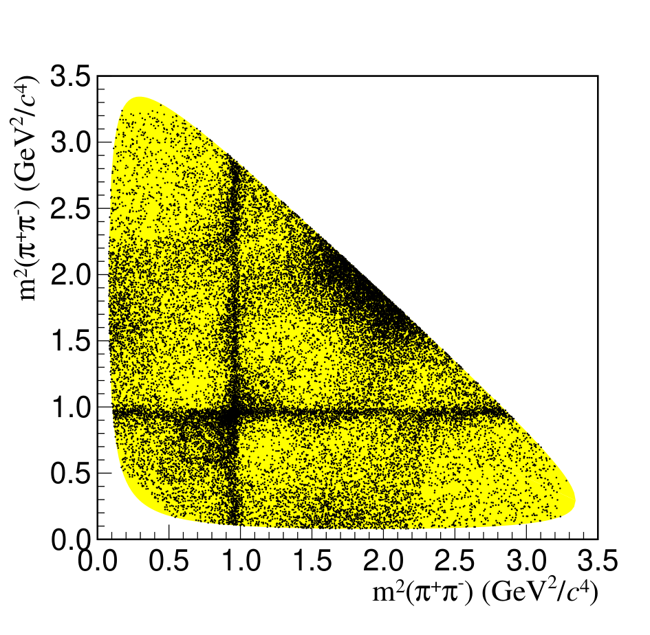Using the track momenta obtained from the $D^{+}_{s}$ mass-constrained kinematic fit, the Dalitz plot symmetrized over particle content for this sample is shown in Fig. 3, where both possible entries from one $D^{+}_{s}$ candidate, ($m^{2}(\pi^{+}\pi^{-})_{\rm low}$, $m^{2}(\pi^{+}\pi^{-})_{\rm high}$) and ($m^{2}(\pi^{+}\pi^{-})_{\rm high}$, $m^{2}(\pi^{+}\pi^{-})_{\rm low}$), are plotted. Here the “low” (“high”) subscript marks the lower (higher) value of the two $\pi^{+}\pi^{-}$ mass combinations. A pair of narrow crossing bands corresponding to the $D^{+}_{s}\rightarrow f_{0}(980)\pi^{+}$ process can be clearly seen. Furthermore, concentration of events around the $m^{2}(\pi^{+}\pi^{-})=1.9$ ${\mathrm{\,Ge\kern-1.00006ptV\!/}c^{2}}$ region is visible, which hints the presence of broad resonances such as $f_{2}(1270)$ and $f_{0}(1370)$.

Figure 1: NN response distributions for (a) direct $D^{+}_{s}$ and (b) indirect $D^{+}_{s}$ categories for data and inclusive MC simulation. The data histograms (points) are compared to MC simulated histograms (lines) including both signal and background (shaded areas) contributions. MC histograms are scaled based on the integrated luminosity of data. The requirements on the NN responses are marked by the vertical dashed lines in red. The $\chi^{2}$ test [21] results for comparison of the data and weighted MC histograms are also shown with ${\rm N}_{\rm bins}$ as the number of histogram bins.

Figure 2: The invariant mass distribution of $D^{+}_{s}\rightarrow\pi^{+}\pi^{-}\pi^{+}$ candidates of data. Data (points) are shown together with the total fit (blue), signal PDF (magenta dashed), and background PDF (light green long dashed). The signal region corresponds to the shaded region, and the sideband events are taken from the cross-hatched regions.

Figure 3: Symmetric Dalitz plot of $D^{+}_{s}\rightarrow\pi^{+}\pi^{-}\pi^{+}$ from data within the signal region. All individual events are shown, with two entries per $D^{+}_{s}$ candidate. The yellow area represents the phase space available to the decay.

IV Amplitude Analysis

This analysis will determine the intermediate-state composition of $D^{+}_{s}\rightarrow\pi^{+}\pi^{-}\pi^{+}$ by analyzing the Dalitz plot of $D^{+}_{s}\rightarrow\pi^{+}\pi^{-}\pi^{+}$ as illustrated in Fig. 3. We randomly assign $m^{2}(\pi^{+}\pi^{-})$ of the two $\pi^{+}\pi^{-}$ combinations in $D^{+}_{s}\rightarrow\pi^{+}\pi^{-}\pi^{+}$ as $x$ and $y$ axes of the Dalitz plot respectively, and the $z$ ($\equiv m^{2}(\pi^{+}\pi^{+})$) axis is used later in efficiency modeling.

IV.1 Analysis formalism

The decay amplitude of $D^{+}_{s}\rightarrow\pi^{+}\pi^{-}\pi^{+}$ is modeled by a coherent sum of various amplitudes with angular momentum quantum numbers $L=0$, $1$, and $2$. Each amplitude $A_{i}$ denoted by $i$ is symmetrized with respect to the two identical pions in the decay,

$${\cal A}_{i}(x,y)=A_{i}(x,y)+A_{i}(y,x).$$ (3)

In our QMIPWA formalism, which is similar to that used by the Fermilab E791 Collaboration to model the $K\pi$ ${\cal S}$ wave [22], the $\pi^{+}\pi^{-}$ ${\cal S}$-wave amplitude is a complex function of $m(\pi^{+}\pi^{-})$. Using the same choice of dividing the $m(\pi^{+}\pi^{-})$ spectrum as in Ref. [2], the ${\cal S}$-wave amplitude $A_{0}(x,y)$ at 29 control points each with an index $k$ is modeled by two real parameters $a_{k}$ (magnitude) and $\gamma_{k}$ (phase). A cubic spline interpolation is used to parametrize both the real and imaginary parts of $A_{0}(x,y)$ for $x_{k}\leq x<x_{k+1}$.

Using the isobar model for ${\cal P}$ waves and ${\cal D}$ waves, the full amplitude is written as a coherent sum of amplitudes ${\cal A}_{i}$ with complex coefficients $c_{i}$,

$${\cal A}(x,y)=\sum_{i}c_{i}{\cal A}_{i}(x,y)\,,$$ (4)

where $c_{0}\equiv 1$, so the free parameters to model the ${\cal S}$-wave amplitude remain unchanged, and the other coefficients $c_{i}\equiv|c_{i}|e^{i\phi_{i}}$ for ${\cal P}$- or ${\cal D}$-wave amplitudes. Each ${\cal P}$- or ${\cal D}$-wave amplitude is represented by the product of Blatt-Weisskopf barrier factors $F_{D_{s},r}^{L}$ [23], a complex relativistic Breit-Wigner function $W^{L}$ and a real spin-dependent angular term $Z^{L}$,

$$A_{i}(x,y)=F_{D}^{L}(x,y)F_{r}^{L}(x,y)W^{L}(x)Z^{L}(x,y)\,.$$ (5)

The detailed formalism is the same as the one in Ref. [24] and therefore left out in the paper.For the Blatt-Weisskopf barrier factors, we set the radii of $D^{+}_{s}$ and intermediate resonances to be $R_{D_{s}}=5$ ${({\mathrm{\,Ge\kern-1.00006ptV\!/}c})}^{-1}$ and $R_{r}=1.5$ ${({\mathrm{\,Ge\kern-1.00006ptV\!/}c})}^{-1}$, respectively.

IV.2 Efficiency

To model the efficiency across the Dalitz plot plane for signal events, we perform an unbinned maximum likelihood fit to the PHSP MC sample with a function $\eta(x,y)={\cal P}(x,y){\cal T}(x){\cal T}(y){\cal T}(z)$ that is symmetric under reflection through $y=x$. Here ${\cal P}(x,y)$ is a two-dimensional polynomial function centered on an arbitrary point ($x_{c}$, $y_{c}$) = (1, 1) GeV²/$c^{4}$ on the Dalitz plot plane,

$${\cal P}(x,y)=1+E_{1}\left(\hat{x}+\hat{y}\right)+E_{2}\left(\hat{x}^{2}+\hat{y}^{2}\right)+E_{11}\hat{x}\hat{y}\\ +E_{3}\left(\hat{x}^{3}+\hat{y}^{3}\right)+E_{12}\left(\hat{x}^{2}\hat{y}+\hat{x}\hat{y}^{2}\right),$$ (6)

where $\hat{x}=x-x_{c}$, $\hat{y}=y-y_{c}$. ${\cal T}(v)$ is a sinelike threshold function for each Dalitz plot variable, $v$ ($\equiv x,y$ or $z$),

$${\cal T}(v)=\left\{\begin{array}[]{ll}\sin(E_{{\rm th},v}\cdot|v-v_{\rm max}|),&E_{{\rm th},v}\cdot|v-v_{\rm max}|<\tfrac{\pi}{2},\\ 1,&E_{{\rm th},v}\cdot|v-v_{\rm max}|\geq\tfrac{\pi}{2},\\ \end{array}\right.$$ (7)

where all polynomial coefficients, $E_{1}$, $E_{2}$, $E_{11}$, $E_{3}$, $E_{12}$, and $E_{{\rm th},v}$ are the fit parameters (requiring $E_{{\rm th},y}\equiv E_{{\rm th},x}$). Each variable $v$ has one threshold, $v_{\rm max}\equiv\left(m_{D_{s}}-m_{\pi}\right)^{2}$, the kinematic limit of $m^{2}(\pi\pi)$, where $m_{\pi}$ is the known mass of $\pi^{+}$. The fit parameters for the efficiency function $\eta(x,y)$ determined in the fit are shown in Table 1. These parameters are fixed in fits to data, and their associated uncertainties are later considered as a source of systematic uncertainties.

Table 1: Fit results of the efficiency function $\eta(x,y)$ from the PHSP MC sample.

Parameter	Value
$E_{1}$	$\phantom{-}0.064\pm 0.003$
$E_{2}$	$-0.066\pm 0.004$
$E_{3}$	$-0.006\pm 0.002$
$E_{11}$	$-0.158\pm 0.006$
$E_{12}$	$\phantom{-}0.090\pm 0.006$
$E_{{\rm th},x(y)}$	$\phantom{-}1.516\pm 0.019$
$E_{{\rm th},z}$	$\phantom{-}1.563\pm 0.028$

IV.3 Likelihood function construction

We perform an unbinned maximum-likelihood fit to the distribution of $D^{+}_{s}$ candidates in the Dalitz plot. The likelihood function is

$${\cal L}=\prod_{{\rm events}}\left\{F\left(m_{j}(D^{+}_{s})\right)\eta\left(x_{j},y_{j}\right)\frac{\left|{\cal A}\left(x_{j},y_{j}\right)\right|^{2}}{\int_{\rm DP}\left|{\cal A}\left(x,y\right)\right|^{2}\eta\left(x,y\right)dxdy}\right.\\ \left.+\left[1-F\left(m_{j}(D^{+}_{s})\right)\right]{\cal B}(x_{j},y_{j})\vphantom{\frac{\sum_{i,j}}{\sum_{i,j}}}\right\}\,,$$ (8)

where

1. $j$ is a $D^{+}_{s}$ candidate index.

2. $F\left(m(D^{+}_{s})\right)$ is the signal fraction, depending on $m(D^{+}_{s})$ before the kinematic fit mentioned in Sec. III. It is defined as

   $$F\left(m(D^{+}_{s})\right)=\frac{{S}\left(m(D^{+}_{s})\right)}{{S}\left(m(D^{+}_{s})\right)+{B}\left(m(D^{+}_{s})\right)}\,,$$

   where ${S}$ and ${B}$ are the signal and background functions determined from fitting to the data mass distribution as depicted in Fig. 2.

3. ${\cal B}(x,y)$ is the background function, which is modeled by a histogram taken from $D^{+}_{s}$ candidates in the data sideband [$1.90<m(D^{+}_{s})<1.93~{\mathrm{\,Ge\kern-1.00006ptV\!/}c^{2}}$ and $2.00<m(D^{+}_{s})<2.0535~{\mathrm{\,Ge\kern-1.00006ptV\!/}c^{2}}$, as shown in Fig. 2]. We also have the normalization requirement $\int{\cal B}(x,y)dxdy=1$.

4. DP is the integral limit denotes the the kinematic limit of the Dalitz plot. The integral is calculated numerically based on a large number of PHSP MC events at the generator level, that is, without the simulation on detector responses.

The fit fraction for the $i$th signal amplitude is defined as

$${\cal F}_{i}=\frac{|c_{i}|^{2}\int|{\cal A}_{i}\left(x,y\right)|^{2}dxdy}{\int\left|{\cal A}\left(x,y\right)\right|^{2}dxdy}\,.$$ (9)

Statistical uncertainties on the fractions include uncertainties on both magnitudes and phases of different signal amplitudes, and are computed using the full covariance matrix.

IV.4 Fitting

Due to the large number of $D^{+}_{s}$ candidates and many parameters involved for the ${\cal S}$-wave parametrization during fitting the Dalitz plot model to the data, an open-source framework called GooFit [25] has been used to speed up the fitting using the parallel processing power of graphical processing units. The cubic spline interpolation method is implemented based on the GooFit framework [26].

V Results of the MIPWA

As in the previous BABAR analysis with similar data sample size, our baseline signal model includes three intermediate resonances with $L\neq 0$: two ${\cal P}$ waves ($\rho(770)$ and $\rho(1450)$) and one ${\cal D}$ wave ($f_{2}(1270)$). The partial wave with $f_{2}(1270)$ is the reference amplitude with the magnitude and phase fixed at 1 and 0, respectively. With the masses and widths of these three resonances fixed to the world averages, and accounting for the magnitude and phase for each of the two $\rho$ resonances and the 29 ${\cal S}$-wave control points relative to the reference amplitude, our baseline signal model contains $N_{\rm par}=62$ free fit parameters. Tables 2 and 3 summarize the results from the amplitude analysis, while the statistical and systematic correlation matrices are given in the Appendix and the Supplemental Material [29]. The fit fraction results in Table 2 show a clear domination of $\pi^{+}\pi^{-}$ ${\cal S}$-wavecontribution. Also, a notable ${\cal D}$-wave contribution from $D^{+}_{s}\rightarrow f_{2}(1270)\pi^{+}$ is found, and the ${\cal P}$-wave contributions from $\rho$ are considerably smaller. Our ${\cal S}$-wave results are also shown in Fig. 4, where at least one resonance around 1 ${\mathrm{\,Ge\kern-1.00006ptV\!/}c^{2}}$ is clearly visible, hinting the presence of $f_{0}(980)$, and contributions from other higher mass scalars such as $f_{0}(1370)$. The comparison with the BABAR measurements shown in Fig. 4 indicates generally good agreement.

Our fit projections are determined by producing a large number of PHSP MC events at the generator level, which are weighted by the fit likelihood function [Eq. (8)], and normalized (with the weighted sum) to the observed number of data candidates. The fit projections are shown in Fig. 5, with the data overlaid for comparison.

Figure 4: (a) Magnitudes and (b) phases of the ${\cal S}$-wave control points as summarized in Table 3. The results are compared to the BABAR results [2] with the same choice on the control points and similar data sample size.

Table 2: Fit fractions, magnitudes, and phases from our baseline fit. The uncertainties are statistical and systematic, respectively. The bottom line shows the sum of all fit fractions. The sum of the fit fractions is not necessarily equal to unity due to the interferences among the contributing amplitudes.

Decay mode	Fit fraction (%)	Magnitude	Phase (radians)
$f_{2}(1270)\pi^{+}$	10.5 $\pm$ 0.8 $\pm$ 1.1	1. (Fixed)	0. (Fixed)
$\rho(770)\pi^{+}$	0.9 $\pm$ 0.4 $\pm$ 0.5	0.13 $\pm$ 0.03 $\pm$ 0.04	5.44 $\pm$ 0.25 $\pm$ 0.60
$\rho(1450)\pi^{+}$	1.3 $\pm$ 0.4 $\pm$ 0.5	0.91 $\pm$ 0.16 $\pm$ 0.21	1.03 $\pm$ 0.32 $\pm$ 0.32
${\cal S}$ wave	84.2 $\pm$ 0.8 $\pm$ 1.2	Table 3	Table 3
$\sum_{i}{\cal F}_{i}$	96.8 $\pm$ 2.4 $\pm$ 3.3

Table 3: Magnitudes and phases of the $\pi^{+}\pi^{-}$ ${\cal S}$-wave control points from our baseline fit. The uncertainties are statistical and systematic, respectively.

Point	Mass (${\mathrm{\,Ge\kern-1.00006ptV\!/}c^{2}}$)	Magnitude	Phase (radians)
1	0.280	$\phantom{0}1.23\pm 1.34\pm 1.73$	$-3.59\pm 1.29\pm 1.19$
2	0.448	$\phantom{0}2.80\pm 0.55\pm 0.62$	$-3.82\pm 0.20\pm 0.21$
3	0.550	$\phantom{0}3.42\pm 0.54\pm 0.62$	$-3.87\pm 0.15\pm 0.14$
4	0.647	$\phantom{0}3.32\pm 0.46\pm 0.42$	$-3.74\pm 0.15\pm 0.13$
5	0.736	$\phantom{0}5.45\pm 0.49\pm 0.60$	$-3.38\pm 0.12\pm 0.09$
6	0.803	$\phantom{0}6.22\pm 0.55\pm 0.61$	$-3.10\pm 0.13\pm 0.14$
7	0.873	$\phantom{0}7.88\pm 0.46\pm 0.66$	$-2.60\pm 0.12\pm 0.09$
8	0.921	$11.85\pm 0.57\pm 0.90$	$-2.16\pm 0.12\pm 0.10$
9	0.951	$16.84\pm 0.80\pm 0.93$	$-1.77\pm 0.11\pm 0.08$
10	0.968	$21.74\pm 1.05\pm 1.41$	$-1.21\pm 0.11\pm 0.09$
11	0.981	$26.45\pm 1.23\pm 1.40$	$-0.58\pm 0.11\pm 0.07$
12	0.993	$18.64\pm 0.89\pm 0.98$	$-0.25\pm 0.10\pm 0.08$
13	1.024	$11.17\pm 0.55\pm 0.44$	$\phantom{-}0.17\pm 0.10\pm 0.07$
14	1.078	$\phantom{0}8.00\pm 0.42\pm 0.17$	$\phantom{-}0.55\pm 0.10\pm 0.05$
15	1.135	$\phantom{0}6.74\pm 0.36\pm 0.22$	$\phantom{-}0.98\pm 0.09\pm 0.07$
16	1.193	$\phantom{0}6.10\pm 0.32\pm 0.46$	$\phantom{-}1.28\pm 0.09\pm 0.03$
17	1.235	$\phantom{0}6.63\pm 0.38\pm 0.53$	$\phantom{-}1.32\pm 0.10\pm 0.03$
18	1.267	$\phantom{0}6.27\pm 0.39\pm 0.42$	$\phantom{-}1.56\pm 0.11\pm 0.09$
19	1.297	$\phantom{0}6.50\pm 0.42\pm 0.25$	$\phantom{-}1.47\pm 0.10\pm 0.06$
20	1.323	$\phantom{0}7.50\pm 0.47\pm 0.38$	$\phantom{-}1.60\pm 0.10\pm 0.06$
21	1.350	$\phantom{0}7.27\pm 0.49\pm 0.69$	$\phantom{-}1.75\pm 0.10\pm 0.11$
22	1.376	$\phantom{0}7.53\pm 0.51\pm 0.45$	$\phantom{-}1.80\pm 0.10\pm 0.12$
23	1.402	$\phantom{0}8.49\pm 0.56\pm 0.68$	$\phantom{-}1.94\pm 0.10\pm 0.07$
24	1.427	$\phantom{0}8.08\pm 0.57\pm 0.56$	$\phantom{-}2.09\pm 0.11\pm 0.09$
25	1.455	$\phantom{0}8.28\pm 0.63\pm 0.63$	$\phantom{-}2.54\pm 0.09\pm 0.09$
26	1.492	$\phantom{0}5.82\pm 0.60\pm 0.61$	$\phantom{-}3.07\pm 0.10\pm 0.12$
27	1.557	$\phantom{0}1.64\pm 0.72\pm 0.79$	$\phantom{-}3.05\pm 0.30\pm 0.56$
28	1.640	$\phantom{0}1.38\pm 0.57\pm 1.06$	$\phantom{-}7.06\pm 0.52\pm 0.78$
29	1.735	$\phantom{0}2.09\pm 0.89\pm 1.70$	$\phantom{-}7.32\pm 0.51\pm 0.60$

Figure 5: Projections of data (points with error bars) and total fit results (blue lines) on (a) total $m^{2}(\pi^{+}\pi^{-})$ (including both $\pi^{+}\pi^{-}$ combinations in a $D^{+}_{s}$ candidate), (b) $m^{2}(\pi^{+}\pi^{+})$, (c) low-mass combination $m^{2}(\pi^{+}\pi^{-})_{\rm low}$, and (d) high-mass combination $m^{2}(\pi^{+}\pi^{-})_{\rm high}$. The shaded areas in cyan are the background contributions. Also shown in (a) and (b) are contributions from the ${\cal S}$ wave (gray long-dashed lines), $\rho(770)$ (yellow dotted lines, scaled by a factor of 10 for better visibility), $\rho(1450)$ (magenta dot-dashed line, scaled by a factor of 10 for better visibility), and $f_{2}(1270)$ (red short-dashed lines).

Figure 6: The $\chi$ distribution across the Dalitz plot using an adaptive binning method.

V.1 Goodness of fit

In order to check the goodness-of-fit of our fit results quantitatively, we use a two-dimensional $\chi^{2}$ test by dividing the Dalitz plot into a number of cells. For the $i$th cell, we have $\chi_{i}=\frac{N_{i}-N_{i}^{\rm exp}}{\sqrt{N_{i}^{\rm exp}}}$, where $N_{i}$ and $N_{i}^{\rm exp}$ are the observed number of $D^{+}_{s}$ candidates and expected number of $D^{+}_{s}$ candidates based on the fit model, respectively. The total $\chi^{2}$ by summing up $\chi^{2}_{i}$ over all cells divided by the number of degrees of freedom ($\nu=N_{\rm cell}-N_{\rm par}$, where $N_{\rm cell}$ is the number of cells having data entries) is used to quantify the fit quality. We calculate $\chi^{2}$ by using an adaptive binning process and requiring the minimal number of entries in each cell is 9, as shown in Fig. 6 for the $\chi_{i}$ values, which leads to $\chi^{2}/\nu=344.4/(404-62)$, with a $\chi^{2}$ probability of $45$%. Figure 6 also indicates generally good data and model agreement across the PHSP.

VI Systematic Uncertainties

We evaluate systematic uncertainties from the following sources, for each source except for the last one the maximum differences between the nominal and varied results are taken as the corresponding systematic uncertainty:

1. The uncertainties arising from the lack of knowledge of the effective barrier radii of mesons are estimated by using alternative values of $R_{D_{s}}$ and $R_{r}$ constants other than the default ones [$5\ {({\mathrm{\,Ge\kern-1.00006ptV\!/}c})}^{-1}$ and $1.5\ {({\mathrm{\,Ge\kern-1.00006ptV\!/}c})}^{-1}$], within the range $[3.0-7.0]\ {({\mathrm{\,Ge\kern-1.00006ptV\!/}c})}^{-1}$ and $[0.0-3.0]\ {({\mathrm{\,Ge\kern-1.00006ptV\!/}c})}^{-1}$, respectively. The variations on $R_{D_{s}}$ and $R_{r}$ values are done one at a time.

2. The uncertainties arising from the uncertainties on the masses and widths of resonances in the baseline model are estimated by varying in turn the masses and widths one standard deviation up and down from world averages.

3. For the uncertainties related to the signal efficiency across the Dalitz plot plane, we vary in turn the coefficients used to parametrize Dalitz plot efficiency listed in Table 1 one standard deviation up and down.

4. For the uncertainties arising from background modeling, instead of the baseline background model, similar to that used in Ref. [2], we use a parametrized background PDF by considering contributions from a $\rho(770)$ meson, two ad hoc scalar resonances with free parameters, and a third order polynomial. The contributions are summed incoherently, and the background PDF parameters are determined by fitting to the sideband data and fixed in the amplitude analysis. In addition, we also model the background contribution using $D^{+}_{s}$ candidates from only the lower or higher sideband regions.

5. The uncertainties arising from modeling of $\rho$ resonances are estimated by performing a fit where the $\rho$ mesons are parametrized instead by the Gounaris-Sakurai formalism [27].

6. As the statistical significance of adding the $\omega(782)\pi^{+}$ contribution in the baseline signal model is below 5$\sigma$, the systematic uncertainties are assigned for those parameters that are common between the two models with and without $\omega(782)\pi^{+}$.

7. The uncertainties related to the signal purity are estimated by scaling the signal fraction [$F\left(m(D^{+}_{s})\right)$ in Eq. (8)] by $\pm 1\%$, which is the uncertainty on the signal purity determined from the $m(D^{+}_{s})$ fit as depicted in Fig. 2.

8. The uncertainties related to the $m(D^{+}_{s})$ signal region are estimated by fitting to a sample of 12,232 data candidates selected within the region of $|\!m(D^{+}_{s})-m_{D_{s}}|<6$ ${\mathrm{\,Me\kern-1.00006ptV\!/}c^{2}}$ and relaxed requirements on the NN responses. The purity is kept at about the same level as the nominal sample (80%).

9. The uncertainties due to the fit procedure are estimated by generating signal MC candidates using the fitted parameters shown in Tables 2 and 3. The signal MC candidates are then mixed with candidates from the inclusive MC sample with signal decays removed to form 35 MC samples, each with total candidate number and signal purity matched to those in data. The parameters of the control points that are close to the Dalitz plot kinematic limits and therefore statistically limited have considerable fit biases, which are about the same size as their statistical uncertainties. We take the mean biases observed when fitting to the MC samples as the related uncertainties.

Furthermore, concerning the choice of control points, the number of control points used for ${\cal S}$-wave modeling has been varied by $\pm 2$ as a consistency check. Also, a fit to data is performed with the ${\cal S}$-wave amplitude parametrized as an interpolation of magnitudes and phases of the 29 control points, instead of their real and imaginary parts as in the baseline fit. As no notable variations for the fit parameters are observed in both cases, no systematic uncertainty is assigned.

Tables 4 and 5 summarize contributions from the different systematic sources. These contributions are combined in quadrature to determine the total systematic uncertainties.

Table 4: Systematic uncertainties for fit fractions and $\rho$ mesons’ coefficients. The dominant systematic uncertainties are highlighted in bold.

	I	II	III	IV	V	VI	VII	VIII	IX	Total
${\cal F}_{f_{2}(1270)}$	${\bf 0.85}$	$0.07$	$0.07$	$0.35$	$0.01$	$0.02$	$0.12$	$0.61$	$0.00$	1.12
${\cal F}_{\rho(770)}$	$0.10$	$0.10$	$0.06$	$0.10$	$0.05$	${\bf 0.44}$	$0.09$	$0.09$	$0.11$	0.51
${\cal F}_{\rho(1450)}$	${\bf 0.42}$	$0.05$	$0.05$	$0.08$	$0.04$	$0.16$	$0.08$	$0.05$	$0.14$	0.49
${\cal F}_{{\cal S}{\rm\,wave}}$	${\bf 0.67}$	$0.04$	$0.10$	$0.56$	$0.06$	$0.02$	$0.33$	$0.64$	$0.44$	1.21
$|c_{\rho(770)}|$	$0.01$	$0.00$	$0.00$	$0.00$	$0.01$	${\bf 0.04}$	$0.01$	$0.00$	$0.01$	0.04
$\phi_{\rho(770)}$ (rad)	$0.09$	$0.03$	$0.04$	$0.26$	$0.01$	${\bf 0.40}$	$0.04$	$0.34$	$0.05$	0.60
$|c_{\rho(1450)}|$	$0.08$	${\bf 0.11}$	$0.02$	$0.04$	$0.10$	$0.05$	$0.03$	$0.05$	$0.06$	0.21
$\phi_{\rho(1450)}$ (rad)	$0.09$	$0.11$	$0.02$	$0.05$	$0.09$	$0.10$	$0.10$	$0.00$	${\bf 0.22}$	0.32

Table 5: Systematic uncertainties for the parameters of the ${\cal S}$-wave control points. The dominant systematic uncertainties are highlighted in bold.

		I	II	III	IV	V	VI	VII	VIII	IX	Total
1	Magnitude	$0.96$	$0.07$	$0.05$	$0.48$	$0.03$	$0.08$	$0.22$	$0.80$	${\bf 1.07}$	1.73
	Phase (rad)	$0.37$	$0.13$	$0.02$	$0.30$	$0.10$	$0.00$	$0.05$	$0.42$	${\bf 0.98}$	1.19
2	Magnitude	$0.34$	$0.05$	$0.05$	$0.31$	$0.03$	$0.05$	$0.15$	$0.10$	${\bf 0.35}$	0.62
	Phase (rad)	${\bf 0.17}$	$0.05$	$0.01$	$0.07$	$0.02$	$0.03$	$0.01$	$0.04$	$0.05$	0.21
3	Magnitude	$0.18$	$0.05$	$0.04$	$0.31$	$0.01$	$0.01$	$0.16$	$0.16$	${\bf 0.45}$	0.62
	Phase (rad)	${\bf 0.12}$	$0.03$	$0.01$	$0.04$	$0.02$	$0.02$	$0.00$	$0.00$	$0.04$	0.14
4	Magnitude	$0.11$	$0.02$	$0.04$	${\bf 0.30}$	$0.03$	$0.14$	$0.15$	$0.18$	$0.02$	0.42
	Phase (rad)	${\bf 0.07}$	$0.03$	$0.01$	$0.05$	$0.02$	$0.06$	$0.00$	$0.05$	$0.04$	0.13
5	Magnitude	$0.26$	$0.03$	$0.05$	${\bf 0.46}$	$0.06$	$0.02$	$0.17$	$0.11$	$0.19$	0.60
	Phase (rad)	$0.04$	$0.01$	$0.01$	$0.01$	$0.02$	$0.02$	$0.02$	$0.01$	${\bf 0.07}$	0.09
6	Magnitude	${\bf 0.43}$	$0.06$	$0.06$	$0.27$	$0.02$	$0.03$	$0.18$	$0.02$	$0.26$	0.61
	Phase (rad)	$0.03$	$0.01$	$0.01$	$0.03$	$0.00$	$0.04$	$0.01$	$0.02$	${\bf 0.12}$	0.14
7	Magnitude	${\bf 0.54}$	$0.07$	$0.04$	$0.22$	$0.00$	$0.26$	$0.13$	$0.03$	$0.06$	0.66
	Phase (rad)	$0.06$	$0.01$	$0.01$	$0.02$	$0.01$	$0.00$	$0.02$	${\bf 0.06}$	$0.03$	0.09
8	Magnitude	${\bf 0.60}$	$0.12$	$0.06$	$0.25$	$0.00$	$0.01$	$0.11$	$0.59$	$0.09$	0.90
	Phase (rad)	$0.06$	$0.02$	$0.00$	$0.01$	$0.01$	$0.02$	$0.01$	$0.02$	${\bf 0.07}$	0.10
9	Magnitude	${\bf 0.65}$	$0.17$	$0.08$	$0.25$	$0.01$	$0.01$	$0.08$	$0.56$	$0.14$	0.93
	Phase (rad)	${\bf 0.05}$	$0.02$	$0.01$	$0.01$	$0.02$	$0.04$	$0.01$	$0.03$	$0.03$	0.08
10	Magnitude	$0.69$	$0.21$	$0.10$	$0.27$	$0.01$	$0.06$	$0.07$	${\bf 1.15}$	$0.21$	1.41
	Phase (rad)	$0.05$	$0.02$	$0.01$	$0.02$	$0.02$	$0.03$	$0.01$	${\bf 0.06}$	$0.01$	0.09
11	Magnitude	$0.72$	$0.25$	$0.11$	$0.25$	$0.00$	$0.09$	$0.07$	${\bf 0.87}$	$0.74$	1.40
	Phase (rad)	${\bf 0.05}$	$0.02$	$0.01$	$0.02$	$0.02$	$0.04$	$0.01$	$0.01$	$0.03$	0.07
12	Magnitude	$0.43$	$0.18$	$0.07$	$0.19$	$0.00$	$0.06$	$0.06$	${\bf 0.83}$	$0.03$	0.98
	Phase (rad)	${\bf 0.05}$	$0.02$	$0.01$	$0.02$	$0.02$	$0.04$	$0.01$	$0.01$	$0.03$	0.08
13	Magnitude	$0.15$	$0.09$	$0.04$	$0.19$	$0.01$	$0.04$	$0.07$	${\bf 0.35}$	$0.03$	0.44
	Phase (rad)	${\bf 0.05}$	$0.01$	$0.00$	$0.02$	$0.02$	$0.03$	$0.00$	$0.01$	$0.04$	0.07
14	Magnitude	$0.06$	$0.06$	$0.02$	${\bf 0.13}$	$0.02$	$0.03$	$0.04$	$0.04$	$0.03$	0.17
	Phase (rad)	$0.02$	$0.01$	$0.00$	$0.03$	$0.01$	${\bf 0.03}$	$0.01$	$0.02$	$0.01$	0.05
15	Magnitude	$0.13$	$0.05$	$0.02$	$0.05$	$0.03$	$0.06$	$0.02$	${\bf 0.14}$	$0.02$	0.22
	Phase (rad)	$0.01$	$0.01$	$0.00$	$0.04$	$0.01$	$0.02$	$0.01$	${\bf 0.05}$	$0.00$	0.07
16	Magnitude	$0.12$	$0.05$	$0.02$	$0.07$	$0.02$	$0.04$	$0.03$	${\bf 0.42}$	$0.10$	0.46
	Phase (rad)	$0.01$	$0.01$	$0.00$	${\bf 0.01}$	$0.01$	$0.01$	$0.00$	$0.00$	$0.01$	0.03
17	Magnitude	$0.17$	$0.06$	$0.02$	$0.07$	$0.01$	$0.04$	$0.03$	${\bf 0.48}$	$0.08$	0.53
	Phase (rad)	${\bf 0.02}$	$0.01$	$0.00$	$0.02$	$0.01$	$0.01$	$0.01$	$0.00$	$0.01$	0.03
18	Magnitude	$0.20$	$0.05$	$0.02$	$0.08$	$0.00$	$0.02$	$0.03$	${\bf 0.36}$	$0.03$	0.42
	Phase (rad)	$0.02$	$0.01$	$0.00$	$0.01$	$0.00$	$0.01$	$0.00$	${\bf 0.08}$	$0.03$	0.09
19	Magnitude	${\bf 0.21}$	$0.05$	$0.02$	$0.08$	$0.02$	$0.02$	$0.04$	$0.06$	$0.03$	0.25
	Phase (rad)	$0.03$	$0.01$	$0.00$	$0.01$	$0.00$	$0.01$	$0.00$	$0.01$	${\bf 0.05}$	0.06
20	Magnitude	${\bf 0.28}$	$0.06$	$0.03$	$0.08$	$0.03$	$0.00$	$0.02$	$0.20$	$0.10$	0.38
	Phase (rad)	${\bf 0.04}$	$0.01$	$0.00$	$0.01$	$0.00$	$0.00$	$0.00$	$0.03$	$0.03$	0.06
21	Magnitude	$0.37$	$0.06$	$0.03$	$0.04$	$0.02$	$0.02$	$0.01$	${\bf 0.57}$	$0.05$	0.69
	Phase (rad)	$0.05$	$0.01$	$0.00$	$0.02$	$0.00$	$0.01$	$0.01$	${\bf 0.07}$	$0.05$	0.11
22	Magnitude	${\bf 0.40}$	$0.07$	$0.03$	$0.03$	$0.02$	$0.02$	$0.00$	$0.15$	$0.12$	0.45
	Phase (rad)	$0.05$	$0.02$	$0.00$	$0.02$	$0.00$	$0.01$	$0.01$	${\bf 0.09}$	$0.06$	0.12
23	Magnitude	${\bf 0.43}$	$0.09$	$0.03$	$0.06$	$0.00$	$0.03$	$0.01$	$0.29$	$0.43$	0.68
	Phase (rad)	${\bf 0.06}$	$0.02$	$0.00$	$0.01$	$0.00$	$0.02$	$0.01$	$0.02$	$0.01$	0.07
24	Magnitude	${\bf 0.44}$	$0.09$	$0.03$	$0.10$	$0.01$	$0.02$	$0.04$	$0.28$	$0.16$	0.56
	Phase (rad)	${\bf 0.07}$	$0.02$	$0.00$	$0.01$	$0.01$	$0.03$	$0.02$	$0.04$	$0.03$	0.09
25	Magnitude	${\bf 0.42}$	$0.10$	$0.04$	$0.14$	$0.02$	$0.04$	$0.04$	$0.26$	$0.35$	0.63
	Phase (rad)	${\bf 0.07}$	$0.02$	$0.00$	$0.01$	$0.01$	$0.03$	$0.02$	$0.02$	$0.02$	0.09
26	Magnitude	$0.30$	$0.09$	$0.04$	$0.15$	$0.00$	$0.10$	$0.06$	${\bf 0.41}$	$0.27$	0.61
	Phase (rad)	${\bf 0.07}$	$0.04$	$0.00$	$0.02$	$0.02$	$0.04$	$0.02$	$0.07$	$0.02$	0.12
27	Magnitude	$0.28$	$0.19$	$0.08$	$0.17$	$0.04$	$0.17$	$0.05$	${\bf 0.64}$	$0.17$	0.79
	Phase (rad)	${\bf 0.32}$	$0.17$	$0.01$	$0.23$	$0.03$	$0.10$	$0.23$	$0.06$	$0.23$	0.56
28	Magnitude	${\bf 0.78}$	$0.19$	$0.05$	$0.23$	$0.12$	$0.13$	$0.14$	$0.08$	$0.60$	1.06
	Phase (rad)	${\bf 0.53}$	$0.09$	$0.06$	$0.06$	$0.03$	$0.07$	$0.17$	$0.48$	$0.21$	0.78
29	Magnitude	$0.43$	$0.09$	$0.05$	$0.15$	$0.05$	$0.42$	$0.24$	$0.34$	${\bf 1.52}$	1.70
	Phase (rad)	${\bf 0.55}$	$0.03$	$0.01$	$0.04$	$0.05$	$0.21$	$0.06$	$0.09$	$0.07$	0.60

VII Conclusion

Based on 3.19 fb^-1 of data taken at $E_{\rm c.m.}=4.178$ GeV with the BESIII detector at the BEPCII collider, we select a sample of 13,797 $D^{+}_{s}\rightarrow\pi^{+}\pi^{-}\pi^{+}$ candidates with a signal purity of 80%. The amplitude analysis shows the decay is dominated by the $\pi^{+}\pi^{-}$ ${\cal S}$ wave. We also observe a significant spin-2 contribution with the fit fraction consistent with that reported by BABAR. Our fit fraction result of ${\cal F}(D^{+}_{s}\rightarrow\rho^{0}\pi^{+})=(0.9\pm 0.4_{\rm stat}\pm 0.5_{\rm syst})\%$ shows a central value somewhat lower than that of the BABAR result, however the two results are still compatible within one standard deviation. Based on the known ${\cal B}(D^{+}_{s}\rightarrow\pi^{+}\pi^{-}\pi^{+})$ [4], we have ${\cal B}(D^{+}_{s}\rightarrow\rho^{0}\pi^{+})={\cal B}(D^{+}_{s}\rightarrow\pi^{+}\pi^{-}\pi^{+})\times{\cal F}(D^{+}_{s}\rightarrow\rho^{0}\pi^{+})=(0.009\pm 0.007)$% that agrees with the predictions in Ref. [28].

As using relativistic Breit-Wigner PDFs to model overlapping intermediate scalars such as $f_{0}(980)$ and $f_{0}(1370)$ will lead to a violation of unitarity and is thus unphysical, the ${\cal S}$-wave content is determined using a quasi-model-independent partial-wave-analysis method. Our results show good agreement with BABAR with a similar data sample size [2]. The statistical uncertainties of our results are generally better than the BABAR ones. As the same choice of control points on the $m(\pi^{+}\pi^{-})$ spectrum is used, combining ${\cal S}$-wave results from both BESIII and BABAR could offer a very precise description of the $\pi^{+}\pi^{-}$ ${\cal S}$ wave in $D^{+}_{s}\rightarrow\pi^{+}\pi^{-}\pi^{+}$, which can be later used to test new models for light scalar resonances.

Appendix A Correlation matrices for the fit fractions

The statistical and systematic correlation matrices for the fit fractions are given in Tables 6 and 7. The statistical and systematic correlation matrices for the 62 fit parameters shown in Table 2 and Table 3 are given in the Supplemental Material [29].

Table 6: Statistical correlation matrix for the fit fractions.

	$f_{2}(1270)\pi^{+}$	$\rho(770)\pi^{+}$	$\rho(1450)\pi^{+}$	${\cal S}$ wave
$f_{2}(1270)\pi^{+}$	$+1.00$	$-0.15$	$-0.30$	$-0.10$
$\rho(770)\pi^{+}$		$+1.00$	$-0.40$	$-0.50$
$\rho(1450)\pi^{+}$			$+1.00$	$+0.27$
${\cal S}$ wave				$+1.00$

Table 7: Systematic correlation matrix for the fit fractions.

	$f_{2}(1270)\pi^{+}$	$\rho(770)\pi^{+}$	$\rho(1450)\pi^{+}$	${\cal S}$ wave
$f_{2}(1270)\pi^{+}$	$+1.00$	$+0.31$	$+0.50$	$-0.04$
$\rho(770)\pi^{+}$		$+1.00$	$-0.16$	$-0.06$
$\rho(1450)\pi^{+}$			$+1.00$	$+0.74$
${\cal S}$ wave				$+1.00$

References

[1] J. M. Link et al. (FOCUS Collaboration), Phys. Lett. B 585, 200 (2004).
[2] B. Aubert et al. (BABAR Collaboration), Phys. Rev. D 79, 032003 (2009).
[3] P. U. E. Onyisi et al. (CLEO Collaboration), Phys. Rev. D 88, 032009 (2013).
[4] P. A. Zyla et al. (Particle Data Group), Prog. Theor. Exp. Phys. 2020, 083C01 (2020).
[5] J. M. Dias, F. S. Navarra, M. Nielsen and E. Oset, Phys. Rev. D 94, 096002 (2016).
[6] H. Y. Cheng, C. W. Chiang and A. L. Kuo, Phys. Rev. D 93, 114010 (2016); H. Y. Cheng and C. W. Chiang, Phys. Rev. D 100, 093002 (2019); 104, 073003 (2021).
[7] P. L. Frabetti et al. (E687 Collaboration), Phys. Lett. B 407, 79 (1997).
[8] E. M. Aitala et al. (E791 Collaboration), Phys. Rev. Lett. 86, 765 (2001).
[9] M. Ablikim et al. (BESIII Collaboration), Nucl. Instrum. Methods Phys. Res., Sect. A 614, 345 (2010).
[10] C. H. Yu et al., Proceedings of IPAC2016, Busan, Korea, 2016, doi:10.18429/JACoW-IPAC2016-TUYA01.
[11] M. Ablikim et al. (BESIII Collaboration), Chin. Phys. C 44, 040001 (2020).
[12] X. Li et al., Radiat. Detect. Technol. Methods 1, 13 (2017); Y. X. Guo et al., Radiat. Detect.Technol. Methods 1, 15 (2017); P. Cao et al., Nucl. Instrum. Meth. A 953, 163053 (2020).
[13] S. Agostinelli et al. (geant4 Collaboration), Nucl. Instrum. Methods Phys. Res., Sect. A 506, 250 (2003).
[14] S. Jadach, B. F. L. Ward and Z. Was, Phys. Rev. D 63, 113009 (2001).
[15] D. J. Lange, Nucl. Instrum. Methods Phys. Res., Sect. A 462, 152 (2001);
R. G. Ping, Chin. Phys. C 32, 599 (2008).
[16] J. C. Chen, G. S. Huang, X. R. Qi, D. H. Zhang and Y. S. Zhu, Phys. Rev. D 62, 034003 (2000);
R. L. Yang, R. G. Ping and H. Chen, Chin. Phys. Lett. 31, 061301 (2014).
[17] E. Richter-Was, Phys. Lett. B 303, 163 (1993).
[18] H. Voss, A. Hoecker, J. Stelzer, and F. Tegenfeldt, Proc. Sci., ACAT 040 (2007); A. Hoecker et al., arXiv:physics/0703039.
[19] M. Ablikim et al. (BESIII Collaboration), Phys. Rev. D 104, 012016 (2021).
[20] T. Skwarnicki, Ph.D. thesis, Institute of Nuclear Physics, Krakow Poland, 1986 [DESY Report No. DESY-F31-86-02, 1986 (unpublished)].
[21] N. D. Gagunashvili, Proc. Sci., ACAT2007 (2007) 054 [arXiv:physics/0605123].
[22] E. M. Aitala et al. (E791 Collaboration), Phys. Rev. D 73, 032004 (2006).
[23] J. M. Blatt and V. F. Weisskopf, Theoretical Nuclear Physics (Wiley, New York, 1951), p. 361.
[24] P. del Amo Sanchez et al. (BABAR Collaboration), Phys. Rev. D 83, 052001 (2011).
[25] R. E. Andreassen, W. M. de Silva, B. T. Meadows, M. D. Sokoloff and K. A. Tomko, IEEE Access 2, 160 (2014).
[26] L. Sun, R. Aoude, A. C. dos Reis and M. D. Sokoloff, J. Phys. Conf. Ser. 898, 072025 (2017).
[27] G. J. Gounaris and J. J. Sakurai, Phys. Rev. Lett. 21, 244 (1968).
[28] Q. Qin, H. n. Li, C. D. Lü and F. S. Yu, Phys. Rev. D 89, 054006 (2014).