Robust Risk-Sensitive Reinforcement Learning Agents for Trading Markets

Abstract

Trading markets represent a real-world financial application to deploy reinforcement learning agents, however, they carry hard fundamental challenges such as high variance and costly exploration. Moreover, markets are inherently a multiagent domain composed of many actors taking actions and changing the environment. To tackle these type of scenarios agents need to exhibit certain characteristics such as risk-awareness, robustness to perturbations and low learning variance. We take those as building blocks and propose a family of four algorithms. First, we contribute with two algorithms that use risk-averse objective functions and variance reduction techniques. Then, we augment the framework to multi-agent learning and assume an adversary which can take over and perturb the learning process. Our third and fourth algorithms perform well under this setting and balance theoretical guarantees with practical use. Additionally, we consider the multi-agent nature of the environment and our work is the first one extending empirical game theory analysis for multi-agent learning by considering risk-sensitive payoffs.

1 Introduction

Reinforcement learning (RL) has moved from toy domains to real-world applications such as games (Berner et al., 2019), navigation (Bellemare et al., 2020), software engineering (Bagherzadeh et al., 2020), industrial design (Mirhoseini et al., 2020), and finance (Li, 2017). Each of these applications has inherent difficulties which are long-standing fundamental challenges in RL, such as: limited training time, costly exploration and safety considerations, among others.

In particular, in finance, there are some examples of RL in stochastic control problems such as option pricing (Li et al., 2009), market making (Spooner et al., 2018), and optimal execution (Ning et al., 2018). However, the most well-known finance application is algorithmic trading, where the goal is to design algorithms capable of automatically making trading decisions based on a set of mathematical rules computed by a machine (Théate & Ernst, 2021).

In algorithmic trading the environment represents the market (and the rest of the actors). The agent’s task is to take actions related to how and how much to trade, and the objective is usually to maximize profit while considering risk. There are diverse challenges in this setting such as partial observability, a large action space, a hard definition of rewards and learning objectives (Théate & Ernst, 2021). In our work we focus on two sought properties for learning agents in realistic scenarios: risk assessment and robustness.

Risk assessment is a cornerstone in financial applications. A well-known approach is to consider risk while assessing the performance (profit) of a trading strategy. Here, risk is a quantity related to the variance (or standard deviation) of the profit and it is commonly refereed to as “volatility”. In particular, the Sharpe ratio (Sharpe, 1994) considers both the generated profit and the risk (variance) associated with a trading strategy. Note that this objective function (Sharpe ratio) is different from traditional RL where the goal is to optimize the expected return, usually, without considerations of risk. There are existing works that proposed risk-sensitive RL algorithms (Mihatsch & Neuneier, 2002; Di Castro et al., 2012) and variance reduction techniques (Anschel et al., 2017). In a similar spirit our proposed algorithms aim to reduce variance while also having convergence guarantees and improved robustness via adversarial learning.

Deep RL has been shown to be brittle in many scenarios (Henderson et al., 2018). Therefore, improving robustness is essential for deploying agents in realistic scenarios. A line of work has improved robustness of RL agents via adversarial perturbations (Morimoto & Doya, 2005; Pinto et al., 2017). In particular, the framework assumes an adversary (who is also learning) who is allowed to take over control at regular intervals. This approach has shown good experimental results in robotics (Pan et al., 2019), and our proposed algorithms extend on this idea while providing convergence guarantees.

Since our motivation is to use RL agents in trading markets (which can be seen as multi-agent interactions) we also evaluate these agents from the perspective of game theory. However, it may be too difficult to analyze in standard game theoretic framework since there is no normal form representation (commonly used to analyze games). Fortunately, empirical game theory (Walsh et al., 2002; Wellman, 2006) overcomes this limitation by using the information of several rounds of repeated interactions and assuming a higher level of strategies (agents’ policies). These modifications have made possible the analysis of multi-agent interactions in complex scenarios such as markets (Bloembergen et al., 2015), and multi-agent games (Tuyls et al., 2020). However, these works have not studied the interactions under risk metrics (such as Sharpe ratio) as we do in this work.

In summary, we take inspiration from previous works to combine risk-awareness, variance reduction and robustness techniques with four different algorithms. Risk-Averse Averaged Q-Learning (RA2-Q) and Variance Reduced Risk-Averse Q-Learning (RA2.1-Q) use risk-averse functions and variance reduction techniques. Then, we augment the framework to a multi-agent scenario where we assume an adversary that can perturb the learning process. We propose Risk-Averse Multi-Agent Q-Learning (RAM-Q) which is a multi-agent version of adversarial learning with strong assumptions and theoretical guarantees. Risk-Averse Adversarial Averaged Q-Learning (RA3-Q) relaxes those assumptions and proposes a more practical algorithm that keeps the multi-agent adversarial component to improve robustness. Lastly, we present a theoretical result using empirical game theory analysis on games with risk-sensitive payoff.

2 Preliminaries

2.1 Single-Agent Reinforcement Learning

A Markov Decision Process is defined by a set of states $\mathcal{S}$ describing the possible configurations, a set of actions $\mathcal{A}$ and a set of observations $\mathcal{O}$ for each agent. A stochastic policy $\pi_{\theta}:\mathcal{O}\times\mathcal{A}\rightarrow[0,1]$ parameterized by $\theta$ produces the next state according to the state transition function $\mathcal{T}:\mathcal{S}\times\mathcal{A}\rightarrow\mathcal{S}$. The agent obtains rewards as a function of the state and agent’s action $r:\mathcal{S}\times\mathcal{A}\rightarrow\mathbb{R}$, and receives a private observation correlated with the state $\mathbf{o}:\mathcal{S}\rightarrow\mathcal{O}$. The initial states are determined by a distribution $d_{0}:\mathcal{S}\rightarrow[0,1]^{|{\mathcal{S}}|}$.

2.2 Multi-Agent Reinforcement Learning

In RL, each agent $i$ aims to maximize its own total expected return, e.g., for a Markov game with two agents, for a given initial state distribution $d_{0}$, the discounted returns are respectively :

$$J^{1}(d_{0},\pi^{1},\pi^{2})=\sum_{t=0}^{\infty}\gamma^{t}\expectation\left[r_{t}^{1}|\pi^{1},\pi^{2},d_{0}\right]$$ (1)

$$J^{2}(d_{0},\pi^{1},\pi^{2})=\sum_{t=0}^{\infty}\gamma^{t}\expectation\left[r_{t}^{2}|\pi^{1},\pi^{2},d_{0}\right]$$ (2)

where $\gamma$ is a discount factor, $r_{t}^{1},r_{t}^{2},\;t=1,2,...$ are respectively immediate rewards for agent 1 & 2. And a Nash equilibrium for Markov game (with two agents) is defined as following

Definition 1.

(Hu & Wellman, 1998) A Nash equilibrium point of game $(J^{1},J^{2})$ is a pair of strategies $(\pi_{*}^{1},\pi_{*}^{2})$ such that for $\forall s\in{\mathcal{S}}$,

$$J^{1}(s,\pi^{1}_{*},\pi^{2}_{*})\geq J^{1}(s,\pi^{1},\pi^{2}_{*})\quad\forall\pi^{1}$$ (3)

$$J^{2}(s,\pi^{1}_{*},\pi^{2}_{*})\geq J^{2}(s,\pi^{1}_{*},\pi^{2})\quad\forall\pi^{2}$$ (4)

2.2.1 Multi-agent Extension of MDP

A Markov game for $N$ agents is defined by a set of states $\mathcal{S}$ describing the possible configurations of all agents, a set of actions $\mathcal{A}_{1},...,\mathcal{A}_{N}$ and a set of observations $\mathcal{O}_{1},...,\mathcal{O}_{N}$ for each agent. To choose actions, each agent $i$ uses a stochastic policy $\pi_{\theta_{i}}:\mathcal{O}_{i}\times\mathcal{A}_{i}\rightarrow[0,1]$ parameterized by $\theta_{i}$, which produces the next state according to the state transition function $\mathcal{P}:\mathcal{S}\times\mathcal{A}_{1}\times...\times\mathcal{A}_{N}\rightarrow\mathcal{S}$. Each agent $i$ obtains rewards as a function of the state and agents’ action $r_{i}:\mathcal{S}\times\mathcal{A}_{1}\times...\times\mathcal{A}_{N}\rightarrow\mathbb{R}$, and receives a private observation correlated with the state $\mathbf{o}_{i}:\mathcal{S}\rightarrow\mathcal{O}_{i}$. The initial states are determined by a distribution $d_{0}:\mathcal{S}\rightarrow[0,1]^{|{\mathcal{S}}|}$. In multi-agent Q learning, the Q tables are defined over joint actions for each of the agents. Each agent receives rewards according to its reward function, with transitions dependent on the actions chosen jointly by the set of agents.

2.3 Empirical Game Theory

We analyze the multi-agent behaviours in a trading market using empirical game theory, where a player corresponds to an agent, and a strategy corresponds to a learning algorithm. Then, in a $p$-player game, players are involved in a single round strategic interaction. Each player $i$ chooses a strategy $\pi^{i}$ from a set of $k$ strategy $S^{i}=\{\pi_{1}^{i},...,\pi_{k}^{i}\}$ and receives a stochastic payoff $R^{i}(\pi^{1},...,\pi^{p}):S^{1}\times S^{2}\times...\times S^{p}\rightarrow\mathbb{R}$. The underlying game that is usually studied is $r^{i}(\pi^{i},...,\pi^{p})=\mathbb{E}[R^{i}(\pi^{1},...,\pi^{p})]$. In general, we denote the payoff of player $i$ as $\mu^{i}$ and $\mathbf{x}^{-i}$ as the joint strategy of all players except for player $i$.

Definition 2.

A joint strategy $\mathbf{x}=(x^{1},...,x^{p})=(x^{i},\mathbf{x}^{-i})$ is a Nash equilibrium if for all $i$ :

$$\mathbb{E}_{\bf{\pi}\sim\mathbf{x}}\left[\mu^{i}(\pi)\right]=\underset{\pi^{i}}{\max}~\mathbb{E}_{\pi^{-i}\sim\mathbf{x}^{-i}}\left[\mu^{i}(\pi^{i},\mathbf{\pi}^{-i})\right]$$ (5)

Definition 3.

A joint strategy $\mathbf{x}=(x^{1},...,x^{p})=(x^{i},\mathbf{x}^{-i})$ is an $\epsilon$-Nash equilibrium if for all $i$:

$$\underset{\pi^{i}}{\max}~\mathbb{E}_{\pi^{-i}\sim\mathbf{x}^{-i}}\left[\mu^{i}(\pi^{i},\mathbf{\pi}^{-i})\right]-\mathbb{E}_{\bf{\pi}\sim\mathbf{x}}\left[\mu^{i}(\pi)\right]\leq\epsilon$$ (6)

Evolutionary dynamics have been used to analyze multi-agent interactions. A well-known model is replicator dynamics (RD) (Weibull, 1997) which describes how a population evolves through time under evolutionary pressure (in our analysis, a population is composed by learning algorithms). RD assumes that the reproductive success is determined by interactions and their outcomes. For example, the population of a certain type increases if they have a higher fitness (in our case this means the expected return in certain interaction) than the population average; otherwise that population share will decrease.

To view the dominance of different strategies, it is common to plot the directional field of the payoff tables using the replicator dynamics for a number of strategy profiles $\mathbf{x}$ in the simplex strategy space (Tuyls et al., 2020). In Section 6.2 we present results in this format evaluating our proposed algorithms.

3 Related Work

Our work is mainly situated in the broad area of safe RL (Garcıa & Fernández, 2015). In particular, a subgroup of works aims to improve robustness of learned policies by assuming two opposing learning processes: one that aims to disturb the most and another one that tries to control the perturbations (Morimoto & Doya, 2005). This approach has been recently adapted to work with neural networks in the context of deep RL (Pinto et al., 2017). Moreover, Risk-Averse Robust Adversarial Reinforcement Learning (RARL) (Pan et al., 2019) extended this idea by combining with Averaged DQN (Anschel et al., 2017), an algorithm that proposes averaging the previous $k$ estimates to stabilize the training process. RARL trains two agents – protagonist and adversary in parallel, and the goal for those two agents are respectively to maximize/minimize the expected return as well as minimize/maximize the variance of expected return. RARL showed good experimental results, but lacked theoretical guarantees and theoretical insights on the variance reduction and robustness. Multi-agent Q-learning (Hu & Wellman, 1998) is useful for finding the optimal strategy when there exists a unique Nash equilibrium in general sum stochastic games, and this approach could also be used in adversarial RL.

Wainwright (2019) proposed a variance reduction Q-learning algorithm (V-QL) which can be seen as a variant of the SVRG algorithm in stochastic optimization (Johnson & Zhang, 2013). Given an algorithm that converges to $Q^{*}$, one of its iterates $\bar{Q}$ could be used as a proxy for $Q^{*}$, and then recenter the ordinary Q-learning updates by a quantity $-\hat{{\mathcal{T}}}_{k}(\bar{Q})+{\mathcal{T}}(\bar{Q})$, where $\hat{{\mathcal{T}}}_{k}$ is an empirical Bellman operator, ${\mathcal{T}}$ is the population Bellman operator, which is not computable, but an unbiased approximation of it could be used instead. This algorithm is shown to be convergent and enjoys minimax optimality up to a logarithmic factor.

Lastly, another group of works proposed the use of risk-averse objective functions (Mihatsch & Neuneier, 2002) with the Q-learning algorithm. Since these ideas are highly related to our proposed algorithms we will describe in greater detail in the next section.

3.1 Risk Averse Q Learning

Shen et al. (2014) proposed a Q learning algorithm that is shown to converge to the optimal of a risk-sensitive objective function, the training scheme is the same as Q learning, except that in each iteration, a utility function is applied to a TD-error (see Algorithm 5 in Appendix).

Since the goal is to optimize the expected return as well as minimizing the variance of the expected return, an expected utility of the return could be used as the objective function instead:

$$\tilde{J}_{\pi}=\frac{1}{\beta}\mathbb{E}_{\pi}\left[exp\left(\beta\sum_{t=0}^{\infty}\gamma^{t}r_{t}\right)\right].$$ (7)

By a straightforward Taylor expansion, Eq. 7 yields

$$\expectation[\sum_{t=0}^{\infty}\gamma^{t}r_{t}]+\frac{\beta}{2}{\mathbb{V}}ar[\sum_{t=0}^{\infty}\gamma^{t}r_{t}]+O(\beta^{2})$$

where when $\beta<0$ the objective function is risk-averse, when $\beta=0$ the objective function is risk-neutral, and when $\beta>0$ the objective function is risk-seeking.

Shen et al. (2014) proved that by applying a monotonically increasing concave utility function $u(x)=-exp(\beta x)$ where $\beta<0$ to the TD error, Algorithm 5 converges to the optimal point of Eq. 7. Hence, it can be shown that:

Theorem 1.

(Theorem 3.2, Shen et al. 2014) Running Algorithm 5 from an initial Q table, $Q\rightarrow Q^{*}$ w.p. 1, where $Q^{*}$ is the unique solution to

$$\expectation_{s^{\prime}}\left[u\left(r(s,a)+\gamma\cdot\underset{a}{\max}Q^{*}(s^{\prime},a)-Q^{*}(s,a)\right)\right]-x_{0}=0$$

$\forall(s,a)$. Where $s^{\prime}$ is sampled from ${\mathcal{T}}[\cdot|s,a]$. And the corresponding policy $\pi^{*}$ of $Q^{*}$ satisfies $\tilde{J}_{\pi^{*}}\geq\tilde{J}_{\pi}\;\forall\pi$.

3.2 Multi-Agent Q-Learning

Hu & Wellman (1998) proposed Nash-Q, a Multi-Agent Q-learning algorithm (Algorithm 6 in Appendix) in the framework of general-sum stochastic games. When there exists a unique Nash equilibrium in the game, this algorithm is useful for finding the optimal strategy. Nash-Q assumes an agent can observe the other agent’s immediate rewards and previous actions during learning. Each learning agent maintains two Q-tables, one for its own Q values, and one for the other agents’. Hu & Wellman (1998) showed that under strong assumptions (Assumption B.3 in Appendix), Nash-Q converges to the Nash Equilibrium. We leave the full version of the algorithm and the convergence theorem to Section B.

Table 1: Comparison of related algorithms. Our proposed algorithms are marked with bold and are described in Section 4.

Algorithm	Description	Guarantees
Risk averse Q-Learning (Shen et al., 2014)	Q-Learning with a utility function applied to TD Error in Q update	Convergence to optimal of a risk-averse objective function
Variance reduced Q-learning (Wainwright, 2019)	Use average estimation of multiple $Q$ tables in Q-table updates to reduce variance	Convergent to optimal of expected return. Convergence rate is minimax optimal up to a logarithmic factor.
Nash Q-learning (Hu & Wellman, 1998)	Two-agent Q-Learning in multi-agent MDP setting	Convergence to Nash equilibrium of the two-agent game (if exists)
Risk-Averse Robust Adversarial Reinforcement Learning (RARL) (Pan et al., 2019)	Q-Learning with risk-averse/risk-seeking behaviors of protagonist/adversary with multiple $Q$ tables	No convergence guarantee
Risk-Averse Averaged Q-Learning (RA2-Q)	Q-Learning with a utility function + a more stable choice of actions with multiple Q tables	Convergence to optimal of a risk-averse objective function and reduced training variance.
Variance Reduced Risk-Averse Q-Learning (RA2.1-Q)	Use average estimation of multiple $Q$ tables in Q updates; Apply utility function in Q updates	No convergence guarantee
Risk-Averse Multiagent Q-learning (RAM-Q)	Multi-agent Nash Q-Learning with a utility function + a risk-averse/risk-seeking behaviors of protagonist/adversary + multiple Q tables	Convergence to Nash equilibrium (if exists) of the two-agent game (with Risk-Averse/Seeking payoffs respectively)
Risk-Averse Adversarial Averaged Q-Learning (RA3-Q)	Multi-agent Q-Learning with a utility function + a risk-averse/risk-seeking behaviors of protagonist/adversary + multiple Q tables	No convergence guarantee

4 Proposed Algorithms

Here we describe our proposed algorithms continuing the results discussed in the previous sections. We first present two algorithms RA2-Q and RA2.1-Q which use a risk-averse utility functions and reduce variance by training multiple Q tables in parallel. Then, we present RAM-Q which is a multi-agent algorithm that assumes an adversary which can perturb the learning process. While RAM-Q is proven to have convergence guarantees, it also needs strong assumptions that might not hold in reality. Therefore, our last proposal, RA3-Q, keeps the adversarial component to improve robustness while relaxing the strong assumptions. As a summary, Table 1 presents closely related works and the comparison with our proposed algorithms.

4.1 Risk-Averse Averaged Q-Learning (RA2-Q)

Algorithm 1 Risk-Averse Averaged Q-Learning (RA2-Q)

Input : Training steps $T$; Exploration rate $\epsilon$; Number of models $k$; risk control parameter $\lambda_{P}$; Utility function parameter $\beta$.

1:  Initialize $Q^{i}=\mathbf{0}$, $N^{i}=\mathbf{0}$, $\alpha^{i}=\mathbf{1}$ for $\forall i=1,...,k$.

2:  Initialize Replay Buffer $RB=\emptyset$; Randomly sample action choosing head integers $H\in[1,k]$

3:  for $t=1$ to $T$ do

4:    $Q=Q^{H}$

5:    Compute $\hat{Q}$ by

$$\hat{Q}(s,a)=Q(s,a)-\lambda_{P}\cdot\frac{\sum_{i=1}^{k}(Q^{i}(s,a)-\bar{Q}(s,a))^{2}}{k-1}$$ (8)

where $\lambda_{P}>0$ is a constant; $\bar{Q}(s,a)=\frac{1}{k}\sum_{i=1}^{k}Q^{i}(s,a)$

6:    Select action $a_{t}$ according to $\hat{Q}$ by applying $\epsilon$-greedy strategy.

7:    Execute actions and get $(s_{t},a_{t},r_{t},s_{t+1})$, append to the replay buffer $RB=RB\cup\{(s_{t},a_{t},r_{t},s_{t+1})\}$

8:    Generate mask $M\in{\mathbb{R}}^{k}\sim Poisson(1)$

9:    for $i=1,...,k$ do

10:     if $M_{i}=1$ then

11:       Update $Q^{i}$ by

$$Q^{i}(s_{t},a_{t})=Q^{i}(s_{t},a_{t})+\alpha^{i}(s_{t},a_{t})\cdot\left[u\left(r(s_{t},a_{t})+\gamma\cdot\underset{a}{\max}Q^{i}(s_{t+1},a)-Q^{i}(s_{t},a_{t})\right)-x_{0}\right]$$ (9)

where $u$ is a utility function, here we use $u(x)=-e^{\beta x}$ where $\beta<0$; $x_{0}=-1$

12:       $N^{i}(s_{t},a_{t})=N^{i}(s_{t},a_{t})+1$; Update learning rate $\alpha^{i}(s_{t},a_{t})=\frac{1}{N^{i}(s_{t},a_{t})}$.

13:     end if

14:    end for

15:    Update $H$ by randomly sampling integers from 1 to $k$.

16:  end for

17:  Return $\frac{1}{k}\sum_{i=1}^{k}Q^{i}$

Although in RAQL (Algorithm 5) we discussed the convergence to the optimal of risk-sensitive objective function with probability 1, the proof assumes visiting every state infinitely many times whereas the actual training time is finite. Our main idea is that we can reduce the training variance further by choosing more risk-averse actions during the finite training process.

Averaged DQN (Anschel et al., 2017) reduces training variance by averaging multiple Q tables in the update. In a similar spirit, our proposed RA2-Q also trains multiple Q tables in parallel. However, we do not directly use the same update rule since that would break the convergence guarantee, in contrast, we train $k$ Q tables in parallel using Eq. 9 as update rule. To select more stable actions we use the sample variance of $k$ Q tables as an approximation to the true variance and then compute a risk-averse $\hat{Q}$ table and select actions according to it. A detailed description is presented in Algorithm 1.

The objective function here is also Eq. 7, and it can be shown that Algorithm 1 also converges to the optimal.

Theorem 2.

Running Algorithm 1 for an initial Q table, then for all $i\in\{1,...,k\}$, $Q^{i}\rightarrow Q^{*}$ w.p. 1, hence the returned table $\frac{1}{k}\sum_{i=1}^{k}Q^{i}\rightarrow Q^{*}$ w.p. 1, where $Q^{*}$ is the unique solution to

$$\expectation_{s^{\prime}}\left[u\left(r(s,a)+\gamma\cdot\underset{a}{\max}Q^{*}(s^{\prime},a)-Q^{*}(s,a)\right)\right]-x_{0}=0$$

for all $(s,a)$. Where $s^{\prime}$ is sampled from ${\mathcal{T}}[\cdot|s,a]$. And the corresponding policy $\pi^{*}$ of $Q^{*}$ satisfies $\tilde{J}_{\pi^{*}}\geq\tilde{J}_{\pi}\;\forall\pi$.

Theorem 2 follows directly from Theorem 1 (see Section C for detail).

4.2 Variance Reduced Risk-Averse Q-Learning (RA2.1-Q)

Algorithm 2 Variance Reduced Risk-Averse Q-Learning (RA2.1-Q)

Input : Training epochs $T$; Exploration rate $\epsilon$; Number of models $k$; Epoch length $K$; Recentering sample size $N$; Utility function parameter $\beta<0$;

1:  Initialize $\bar{Q}_{0}=\mathbf{0}$; $m=1$; $RB=\emptyset$.

2:  for $m=1$ to $T$ do

3:    Select action according to $\bar{Q}_{m-1}$ by applying $\epsilon-$greedy strategy

4:    Execute action and get $(s,a,r(s,a),s^{\prime})$ and update the replay buffer $RB=RB\cup(s,a,r(s,a),s^{\prime})$.

5:    for $i=1,...,N$ do

6:     Define the empirical Bellman operator $\ddot{\mathcal{T}_{i}}$ as

$$\ddot{\mathcal{T}_{i}}(Q)(s,a)=u\left(r(s,a)+\gamma\cdot\underset{a^{\prime}}{\max}\;Q(s_{i},a^{\prime})\right)-x_{0}$$

   where $s_{i}$ is randomly sampled from ${\mathcal{T}}[\cdot|s,a]$; $u$ is the utility function, and $u(x)=-e^{\beta x}$, $\beta<0$ and $x_{0}=-1$

7:    end for

8:    Define $\tilde{\mathcal{T}}_{N}(\bar{Q}_{m-1})=\frac{1}{N}\sum_{i\in\mathcal{D}_{N}}\ddot{\mathcal{T}_{i}}(\bar{Q}_{m-1})$, where $\mathcal{D}_{N}$ is a collection of $N$ i.i.d. samples (i.e., matrices with samples for each state-action pair $(s,a)$ from $RB$).

9:    Define $Q_{1}=\bar{Q}_{m-1}$.

10:    for $k=1,...,K$ do

11:     Compute stepsize $\lambda_{k}=\frac{1}{1+(1-\gamma)k}$

12:     

$$Q_{k+1}=(1-\lambda_{k})\cdot Q_{k}+\lambda_{k}\cdot\left[\ddot{\mathcal{T}_{k}}(Q_{k})-\ddot{\mathcal{T}_{k}}(\bar{Q}_{m-1})+\tilde{\mathcal{T}}_{N}(\bar{Q}_{m-1})\right].$$ (10)

where $\ddot{\mathcal{T}_{k}}$ is empirical Bellman operator constructed using a sample not in $\mathcal{D}_{N}$, thus the random operators $\ddot{\mathcal{T}_{k}}$ and $\tilde{\mathcal{T}}_{N}$ are independent

13:    end for

14:    $\bar{Q}_{m}=Q_{K+1}$; $m$ = $m+1$

15:  end for

16:  Return $\bar{Q}_{m}$

Wainwright (2019) proposed Variance Reduced Q-learning which trains multiple Q tables in parallel and uses the averaged Q table in the update rule. It is shown that it guarantees a convergence rate which is minimax optimal. Inspired by that work, we propose our RA2.1-Q (Algorithm 2) which applies a utility function to the TD error during Q updates for the purpose of further reducing variance. To select more stable actions during training, we use the sample variance of $k$ Q tables as an approximation to the true variance and then compute a risk-averse $\hat{Q}$ table and select actions according to it. We’ll discuss more details in Section 7.

4.3 Multi-Agent Risk-Averse Q-Learning (RAM-Q)

Algorithm 3 Risk-Averse Multi-Agent Q-Learning (RAM-Q)

Input : Training steps $T$; Exploration rate $\epsilon$; Number of models $k$; Utility function parameters $\beta^{P}<0;\beta^{A}>0$.

1:  For $\forall(s,a_{P},a_{A})$, initialize $Q^{P}(s,a_{P},a_{A})=0$; $Q^{A}(s,a_{P},a_{A})=0$; $N(s,a_{P},a_{A})=0$.

2:  for $t=1$ to $T$ do

3:    At state $s_{t}$, compute $\pi^{P}(s_{t})$, $\pi^{A}(s_{t})$, which is a mixed strategy Nash equilibrium solution of the bimatrix game $(Q^{P}(s_{t}),Q^{A}(s_{t}))$.

4:    Choose action $a_{t}^{P}$ based on $\pi^{P}(s_{t})$ according to $\epsilon$-greedy and choose action $a_{t}^{A}$ based on $\pi^{A}(s_{t})$ according to $\epsilon$-greedy

5:    Observe $r_{t}^{P},r_{t}^{A}$ and $s_{t+1}$.

6:    At state $s_{t+1}$, compute $\pi^{P}(s_{t+1})$,$\pi^{A}(s_{t+1})$, which are mixed strategies Nash equilibrium solutions of the bimatrix game $(Q^{P}(s_{t+1}),Q^{A}(s_{t+1}))$.

7:    $N(s_{t},a^{P}_{t},a^{A}_{t})=N(s_{t},a^{P}_{t},a^{A}_{t})+1$

8:    Set learning rate $\alpha_{t}=\frac{1}{N(s_{t},a^{P}_{t},a^{A}_{t})}$.

9:    Update $Q^{P},Q^{A}$ such that

$$Q^{P}(s_{t},a^{P}_{t},a^{A}_{t})=Q^{P}(s_{t},a^{P}_{t},a^{A}_{t})+\alpha_{t}\cdot\left[u^{P}\left(r_{t}^{P}+\gamma\cdot\pi^{P}(s_{t+1})Q^{P}(s_{t+1})\pi^{A}(s_{t+1})-Q^{P}(s_{t},a^{P}_{t},a^{A}_{t})\right)-x_{0}\right]$$ (11)

where $u^{P}$ is a utility function, here we use $u^{P}(x)=-e^{\beta^{P}x}$ where $\beta^{P}<0$; $x_{0}=-1$.

$$Q^{A}(s_{t},a^{P}_{t},a^{A}_{t})=Q^{A}(s_{t},a^{P}_{t},a^{A}_{t})+\alpha_{t}\cdot\left[u^{A}\left(r_{t}^{A}+\gamma\cdot\pi^{P}(s_{t+1})Q^{A}(s_{t+1})\pi^{A}(s_{t+1})-Q^{A}(s_{t},a^{P}_{t},a^{A}_{t})\right)-x_{1}\right]$$ (12)

where $u^{A}$ is a utility function, here we use $u^{A}(x)=e^{\beta^{A}x}$ where $\beta^{A}>0$; $x_{1}=1$.

10:  end for

11:  Return $(Q^{P},Q^{A})$

In complex scenarios such as financial markets learned RL policies can be brittle. To improve robustness, we adapt ideas from adversarial learning to a multi-agent learning problem similar to (Hu & Wellman, 1998).

In the adversarial setting we assume there are two learning processes happening simultaneously, a main protagonist (P) and an adversary (A): the goal of protagonist is to maximize the total return as well as minimize the variance; the goal of adversary is to minimize the total return of protagonist as well as maximizing the variance. Here, we assume that each agent can observe its opposite’s immediate reward.

Let $r_{t}^{P}$ be the immediate reward received by protagonist at step $t$, and let $r_{t}^{A}$ be the immediate reward received by adversary at step $t$. Then we choose the objective functions as follows:

The objective function for the protagonist is,

$$\tilde{J}_{\pi}^{P}=\frac{1}{\beta^{P}}\expectation_{\pi}\left[exp\left(\beta^{P}\sum_{t=0}^{\infty}\gamma^{t}\cdot r_{t}^{P}\right)\right]\qquad\beta^{P}<0$$ (13)

by a Taylor expansion, Eq. 13 yields,

$$\tilde{J}_{\pi}^{P} =\expectation\left[\sum_{t=0}\gamma^{t}\cdot r_{t}^{P}\right]+\frac{\beta^{P}}{2}{\mathbb{V}}ar\left[\sum_{t=0}\gamma^{t}\cdot r_{t}^{P}\right]+O((\beta^{P})^{2}).$$

Similarly, the objective function for the adversary is,

$$\tilde{J}_{\pi}^{A}=\frac{1}{\beta^{A}}\expectation_{\pi}\left[exp\left(\beta^{A}\sum_{t=0}^{\infty}\gamma^{t}r_{t}^{A}\right)\right]\qquad\beta^{A}>0$$ (14)

and by Taylor expansion, Eq. 14 yields,

$$\tilde{J}_{\pi}^{A}= \expectation\left[\sum_{t=0}\gamma^{t}\cdot r_{t}^{A}\right]+\frac{\beta^{A}}{2}{\mathbb{V}}ar\left[\sum_{t=0}\gamma^{t}\cdot r_{t}^{A}\right]+O((\beta^{A})^{2}).$$

Using the same spirit in (Hu & Wellman, 1998), we proposed Algorithm 3 and the following guarantee holds :

Theorem 3.

If the two-agent game $(\tilde{J}^{P},\tilde{J}^{A})$ has a Nash equilibrium solution, then running Algorithm 3 from initial Q tables $Q^{P},Q^{A}$ will converge to $Q_{P}^{*}$ and $Q_{A}^{*}$ w.p. 1. s.t. the Nash equilibrium solution $(\pi^{P}_{*},\pi^{A}_{*})$ for the bimatrix game $(Q_{P}^{*},Q_{A}^{*})$ is the Nash equilibrium solution to the game $(\tilde{J}^{P}_{\pi},\tilde{J}^{A}_{\pi})$, and the equilibrium payoff are $\tilde{J}^{P}(s,\pi^{P}_{*},\pi^{A}_{*})$, $\tilde{J}^{A}(s,\pi^{P}_{*},\pi^{A}_{*})$.

Although Theorem 3 gives a solid convergence guarantee, it suffers from drawbacks like expensive computational cost and idealized assumptions, e.g., in trading markets, there may not exist a Nash equilibrium to $(\tilde{J}^{P},\tilde{J}^{A})$, and during the training process, assumptions about the Nash equilibrium (Assumption B.3 in Appendix) break easily (Bowling, 2000). Hence, we design another novel algorithm RA3-Q which relaxes these assumptions (at the expense of loosing theoretical guarantees) while enhancing robustness and performing well in reality.

4.4 Risk-Averse Adversarial Averaged Q-Learning (RA3-Q)

Algorithm 4 Risk-Averse Adversarial Averaged Q-Learning (RA3-Q) Short Version

Input : Training steps $T$; Exploration rate $\epsilon$; Number of models $k$; Risk control parameters $\lambda_{P},\lambda_{A}$; Utility function parameters $\beta^{P}<0;\beta^{A}>0$.

1:  Initialize $Q_{P}^{i},Q_{A}^{i}\;\forall i=1,...,k$; $N=\mathbf{0}\in{\mathbb{R}}^{|{\mathcal{S}}|\times|{\mathcal{A}}|\times|{\mathcal{A}}|}$. Randomly sample action choosing head integers $H_{P},H_{A}\in\{1,...,k\}$.

2:  for $t=1$ to $T$ do

3:    Set $Q_{P}=Q_{P}^{H_{P}}$. Then compute $\hat{Q}_{P}$, the risk-averse protagonist $Q$ table by the $k$ Q tables $Q_{P}^{i},i=1,...,k$.

4:    Set $Q_{A}=Q_{A}^{H_{A}}$. Then compute $\hat{Q}_{A}$, the risk-seeking protagonist $Q$ table by the $k$ Q tables $Q_{A}^{i},i=1,...,k$.

5:    Select actions $a_{P},a_{A}$ according to $\hat{Q}_{P},\hat{Q}_{A}$ by applying $\epsilon$-greedy strategy.

6:    Generate mask $M\in{\mathbb{R}}^{k}\sim Poisson(1)$ and update $Q_{P}^{i},Q_{A}^{i},i=1,...,k$ according to mask $M$ using update rules Eq. 82 and Eq. 83.

7:    Update $H_{P}$ and $H_{A}$

8:  end for

9:  Return $\frac{1}{k}\sum_{i=1}^{k}Q_{P}^{i}$; $\frac{1}{k}\sum_{i=1}^{k}Q_{A}^{i}$.

We start from the same objective functions for the protagonist, Eq. 13, and adversary, Eq. 14. In order to optimize $\tilde{J}^{P}$ and $\tilde{J}^{A}$, we apply utility functions to TD errors when updating Q tables, and combining the idea of training multiple Q tables in parallel as Algorithm 1 to select actions with low variance, we get a novel Algorithm 4 (full version Algorithm 7 in Section E).

Note that RA3-Q combines (i) risk-averse using utility functions (ii) variance reduction by training multiple Q tables and (iii) robustness by adversarial learning. Intuitively, as the adversary is getting stronger, the protagonist experiences harder challenges, thus enhancing robustness. Compared to Algorithm 3, where the returned policy $(\pi^{P},\pi^{A})$ is a Nash equilibrium of the $(\tilde{J}^{P},\tilde{J}^{A})$, Algorithm 4 does not have a convergence guarantee, however, it has several practical advantages including computational efficiency, simplicity (no strong assumptions) and more stable actions during training. For a longer discussion see Section 7 and Section E.

5 Performance Evaluated by Empirical Game Theory

When the environment is populated by many learning agents, how do we evaluate their performance and decide which strategy is the best? Although different approaches can be used, we focused on empirical game theory (EGT) to address this question.

In EGT each agent is a player involved in rounds of strategic interaction (games). By meta-game analysis, we can evaluate the superiority of each strategy. Our contribution is to theoretically prove that the Nash-Equilibrium of risk averse meta-game is an approximation of the Nash-Equilibrium of the population game, to our knowledge, this is the first work doing this type of risk-averse analysis.

5.1 Replicator dynamics

In EGT, we can visualize the dominance of strategies by plotting the meta-game payoff tables together with the replicator dynamics. A meta game payoff table could be seen as a combination of two matrices $(N|R)$, where each row $N_{i}$ contains a discrete distribution of $p$ players over $k$ strategies, and each row yields a discrete profile $(n_{\pi_{1}},...,n_{\pi_{k}})$ indicating exactly how many players play each strategy with $\sum_{j}n_{\pi_{j}}=p$. A strategy profile $\mathbf{u}=\left(\frac{n_{\pi_{1}}}{p},...,\frac{n_{\pi_{k}}}{p}\right)$. And each row $R_{i}$ captures the rewards corresponding to the rows in $N$.

For example, for a game $A$ with 2 players, and 3 strategies $\{\pi_{1},\pi_{2},\pi_{3}\}$ to choose from, the meta game payoff table could be constructed as follows : In the left side of the table, we list all of the possible combinations of strategies. If there are $p$ players and $k$ strategies, then there are $\binom{p+k-1}{p}$ rows, hence in game $A$, there are 6 rows. See Section F for a concrete example.

Once we have a meta-game payoff table and the replicator dynamics, a directional field plot is computed where arrows in the strategy space indicates the direction of flow, or change, of the population composition over the strategies (see Section F for two examples of directional field plots in multi-agent problems). In Section 6.2 we present trading market experiments and results based on meta-game analysis with the performance of RAQL, RA2-Q and RA2.1-Q.

5.2 Nash Equilibrium with risk neutral payoff

Previously, Tuyls et al. (2020) showed that for a game $r^{i}(\pi^{i},...,\pi^{p})=\expectation[R^{i}(\pi^{1},...,\pi^{p})]$, with a meta-payoff (empirical payoff) $\hat{r}^{i}(\pi^{i},...,\pi^{p})$, the Nash Equilibrium of $\hat{r}$ is an approximation of Nash Equilibrium of $r$.

Lemma 1.

(Tuyls et al., 2020) If $\mathbf{x}$ is a Nash Equilibrium for the game $\hat{r}^{i}(\pi^{1},...,\pi^{p})$, then it is a $2\epsilon$-Nash equilibrium for the game $r^{i}(\pi^{1},...,\pi^{p})$, where $\epsilon=\underset{\pi,i}{sup}~|\hat{r}^{i}(\pi)-r^{i}(\pi)|$.

Lemma 1 implies that if for each player, we can bound the estimation error of empirical payoff, then we can use the Nash Equilibrium of meta game as an approximation of Nash Equilibrium of the game.

5.3 Risk averse payoff EGT

Recall our objective is to consider risk averse payoff to evaluate strategies. Hence, instead of letting

$$r^{i}(\pi^{i},...,\pi^{p})=\mathbb{E}[R^{i}(\pi^{1},...,\pi^{p})],$$

we choose

$$h^{i}(\pi^{i},...,\pi^{p})=\mathbb{E}[R^{i}(\pi^{1},...,\pi^{p})]-\beta\cdot\mathbb{V}ar[R^{i}(\pi^{1},...,\pi^{p})]$$

(where $\beta>0$) as the game payoff. Moreover, we use

$$\hat{h}^{i}(\pi^{i},...,\pi^{p})=\bar{R^{i}}-\beta\cdot\left[\frac{1}{n-1}\sum_{j=1}^{n}\left(R^{i}_{j}-\bar{R^{i}}\right)^{2}\right]$$ (15)

as meta-game payoff, where $\bar{R^{i}}=\frac{1}{n}\sum_{j=1}^{n}R^{i}_{j}$ and $R_{j}^{i}$ is the stochastic payoff of player $i$ in $j-$th experiment. To our knowledge, there is no previous work on empirical game theory analysis with risk sensitive payoff. Below we give the first theoretical analysis showing that for our risk-averse payoff game, we can still approximate the Nash Equilibrium by meta game.

Theorem 4.

Under Assumption G.4, for a Normal Form Game with $p$ players, and each player $i$ chooses a strategy $\pi^{i}$ from a set of strategies $S^{i}=\{\pi^{i}_{1},...,\pi^{i}_{k}\}$ and receives a meta payoff $h^{i}(\pi^{1},...,\pi^{p})$ (Eq. 15). If $\mathbf{x}$ is a Nash Equilibrium for the game $\hat{h}^{i}(\pi^{1},...,\pi^{p})$, then it is a $2\epsilon$-Nash equilibrium for the game $h^{i}(\pi^{1},...,\pi^{p})$ with probability $1-\delta$ if we play the game for $n$ times, where

$$\begin{split}n\geq\max\left\{-\frac{8R^{2}}{\epsilon^{2}}\log\left[\frac{1}{4}\left(1-(1-\delta)^{\frac{1}{|S^{1}|\times...\times|S^{p}|\times p}}\right)\right],\right.\\ \left.\frac{64\beta^{2}\omega^{2}\cdot\Gamma(2)}{\epsilon^{2}\left[1-(1-\delta)^{\frac{1}{|S^{1}|\times...\times|S^{p}|\times p}}\right]}\right\}\end{split}$$ (16)

6 Experiments

6.1 Setup

Our experiments use the open-sourced ABIDES (Byrd et al., 2019) market simulator in a simplified setting. The environment is generated by replaying publicly available real trading data for a single stock ticker. The setting is composed of one non-learning agent that replays the market deterministically (Balch et al., 2019) and learning agents. The learning agents considered are: RAQL, RA2-Q, RA2.1-Q, and RA3-Q.

We follow a similar setting to existing implementations in ABIDES where the state space is defined by two features: current holdings and volume imbalance. Agents take one action at every time step (every second) selecting among: buy/sell with limit price $base+i\cdot K$, where $i\in\{1,2,..,6\}$ or do nothing. The immediate reward is defined by the change in the value of our portfolio (mark-to-market) and comparing against the previous time step. Our comparisons are in terms of Sharpe ratio, which is a widely used measure in trading markets.

6.2 Risk and robustness evaluation

Table 2: Meta-payoff of 2 players, 3 strategies, respectively RAQL (Shen et al., 2014), RA2-Q and RA2.1-Q over 80 simulations. The return here used is Sharpe Ratio.

$N_{i1}$	$N_{i2}$	$N_{i3}$	$R_{i1}$	$R_{i2}$	$R_{i3}$
2	0	0	0.9130	0	0
1	1	0	0.7311	0.7970	0
0	2	0	0	1.0298	0
1	0	1	0.6791	0	1.0786
0	0	2	0	0	2.2177
0	1	1	0	0.7766	1.4386

Figure 1: (a) Directional field plot and (b) Trajectory plot of the simplex of 3 strategies based on the meta-game payoff from Table 2. It can be seen that RA2.1-Q (top) is the the strongest attractor. White circles represent equilibria.

Table 2 shows the meta-payoff table of a two player-game among three strategies: RAQL, RA2-Q and RA2.1-Q. The results show that our two proposed algorithms RA2-Q and RA2.1-Q obtained better results than RAQL. With those payoffs we obtained the directional and trajectory plots shown in Fig. 1, where black solid circles denote globally-stable equilibria, and the white circles denote unstable equilibria (saddle-points), in (a) the plot is colored according to the speed at which the strategy mix is changing at each point; in (b) the lines show trajectories for some points over the simplex.

Table 3: Comparison in terms for Sharpe ratio with two types of perturbations: The trained adversary from RA3-Q is used in testing time. Zero-intelligence agents are added to the simulation to perturb the market. RA3-Q obtains better results in both cases due to its enhanced robustness.

Algorithm/Setting	Adversarial Perturbation	ZI Agents Perturbation
RA2-Q	0.5269	0.9538
RA3-Q	0.9347	1.0692

Our last experiment compares RA2-Q and RA3-Q in terms of robustness. In this setting we trained both agents under the same conditions as a first step. Then in testing phase we added two types of perturbations, one adversarial agent (trained within RA3-Q) or adding noise (aka. zero-intelligence) agents in the environment. In both cases, the agents will act in a perturbed environment. The results are presented in Table 3 in terms of Sharpe ratio using cross validation with 80 experiments.

7 Discussion

Here we briefly discuss some trade-offs between practical and theoretical results about our proposed algorithms.

As mentioned in Section 4.2, we did not show that Algorithm 2 (RA2.1-Q) has a convergence guarantee, however, it obtained good empirical results (better than RAQL and RA2-Q). It is an open question whether RA2.1-Q converges to the optimal of Eq. 7, furthermore, it could be interesting to study whether it also enjoys minimax optimality convergence rate up to a logarithmic factor as in (Wainwright, 2019). Similarly, RA3-Q does not have a convergence guarantee in the multi-agent learning scenario (when protagonist and adversary are learning simultaneously). However, RA3-Q obtained better empirical results than RA2-Q highlighting its robustness. In Section E we show a related result showing that Eq. 82 or Eq. 83 converge to optimal assuming the policy for the adversary (or protagonist) is fixed (thus, it is no longer a multi-agent learning setting).

On the side of EGT analysis, previous works used average as payoff (Tuyls et al., 2020) and our work considers a risk-averse measure based on variance (second moment), studying higher moments and other measures is one interesting open question.

8 Conclusions

We have proposed 4 different Q-learning style algorithms that augment reinforcement learning agents with risk-awareness, variance reduction, and robustness. RA2-Q and RA2.1-Q are risk-averse but use slightly different techniques to reduce variance. RAM-Q and RA3-Q are two proposals that extend by adding an adversarial learning layer which is expected to improve its robustness. On the one side, our theoretical results show convergence results for RA2-Q and RAM-Q, on the other side, in our empirical results RA2.1-Q and RA3-Q obtained better results in a simplified trading scenario. Lastly, we contributed with risk-averse analysis of our algorithms using empirical game theory. As future work we want to perform a more extensive set of experiments to evaluate the algorithms under different conditions.

Appendix

A Risk-Averse Q-Learning (RAQL) and proof of convergence

Algorithm 5 Risk-Averse Q-Learning (RAQL) (Shen et al., 2014)

1:  For $\forall(s,a)$, initialize $Q(s,a)=0$; $N(s,a)=0$.

2:  for $t=1$ to $T$ do

3:    At state $s_{t}$, choose action according to the $\epsilon$-greedy strategy.

4:    Observe $s_{t},a_{t},r_{t},s_{t+1}$

5:    $N(s_{t},a_{t})=N(s_{t},a_{t})+1$

6:    Set learning rate $\alpha_{t}=\frac{1}{N(s_{t},a_{t})}$

7:    Update Q :

$$Q_{t+1}(s_{t},a_{t})=Q_{t}(s_{t},a_{t})+\alpha_{t}(s_{t},a_{t})\cdot\left[u\left(r_{t}+\gamma~\cdot\underset{a}{\max}Q_{t}(s_{t+1},a)-Q_{t}(s_{t},a_{t})\right)-x_{0}\right]$$ (17)

where $u$ is a utility function, here we use $u(x)=-e^{\beta x}$ where $\beta<0$; $x_{0}=-1$

8:  end for

9:  Return Q.

A.1 Proof of Theorem 1

This proof is originally proved by (Shen et al., 2014), but we describe it here in detail because it will be useful for later proofs for our proposed algorithms.

First, we show the following Lemma :

Lemma A.2.

For the iterative procedure

$$Q_{t+1}(s_{t},a_{t})=Q_{t}(s_{t},a_{t})+\alpha_{t}(s_{t},a_{t})\left[u\left(r_{t}+\gamma\cdot\underset{a}{\max}Q_{t}(s_{t+1},a)-Q_{t}(s_{t},a_{t})\right)-x_{0}\right]$$ (18)

where $\alpha_{t}\geq 0$ satisfy that for any $(s,a)$, $\sum_{t=0}^{\infty}\alpha_{t}(s,a)=\infty$; and $\sum_{t=0}^{\infty}\alpha^{2}_{t}(s,a)<\infty$, then $Q_{t}\rightarrow Q^{*}$, where $Q^{*}$ is the solution of the Bellman equation

$$(H^{A}Q^{*})(s,a)=\alpha\cdot\expectation_{s,a}\left[\tilde{u}\left(r_{t}+\gamma\cdot\underset{a}{\max}Q^{*}(s_{t+1},a)-Q^{*}(s,a)\right)\right]+Q^{*}(s,a)=Q^{*}(s,a)\qquad\forall(s,a)$$ (19)

If Lemma A.2 holds, then it’s shown in (Shen et al., 2014) that the corresponding policy optimizes the objective function Eq. 7.

A.2 Proof of Lemma A.2

Before proving the convergence, we consider a more general update rule

$$q_{t+1}(i)=(1-\alpha_{t}(i))q_{t}(i)+\alpha_{t}(i)\left[(Hq_{t})(i)+w_{t}(i)\right]$$ (20)

where $i$ is the independent variable (e.g., in single agent Q learning, it’s the state-action pair $(s,a)$), $q_{t}\in{\mathbb{R}}^{d}$, $H:{\mathbb{R}}^{d}\rightarrow{\mathbb{R}}^{d}$ is an operator, $w_{t}$ denotes some random noise term and $\alpha_{t}$ is learning rate with the understanding that $\alpha_{t}(i)=0$ if $q(i)$ is not updated at time $t$. Denote by ${\mathcal{F}}_{t}$ the history of the algorithm up to time $t$,

$${\mathcal{F}}_{t}=\{q_{0}(i),...,q_{t}(i),w_{0}(i),...,w_{t}(i),\alpha_{0}(i),...,\alpha_{t}(i)\}$$ (21)

Recall the following essential proposition :

Proposition A.1.

(Bertsekas, 2009) Let $q_{t}$ be the sequence generated by the iteration Eq. 20, if we assume the following hold :

1. The Learning rates $\alpha_{t}(i)$ satisfy :

   $$\alpha_{t}(i)\geq 0;\qquad\sum_{t=0}^{\infty}\alpha_{t}(i)=\infty;\qquad\sum_{t=0}^{\infty}\alpha_{t}^{2}(i)<\infty;\quad\forall i$$ (22)

2. The noise terms $w_{t}(i)$ satisfy

   1. $\expectation[w_{t}(i)|{\mathcal{F}}_{t}]=0$ for all $i$ and $t$;

   2. There exist constants $A$ and $B$ such that $\expectation[w_{t}^{2}(i)|{\mathcal{F}}_{t}]\leq A+B\left\|q_{t}\right\|^{2}$ for some norm $\left\|\cdot\right\|$ on ${\mathbb{R}}^{d}$.

3. The mapping $H$ is a contraction under sup-norm.

Then $q_{t}$ converges to the unique solution $q^{*}$ of the equation $Hq^{*}=q^{*}$ with probability 1.

In order to apply Proposition A.1, we reformulate the update rule Eq. 9 by letting

$$q_{t+1}(s,a)=\left(1-\frac{\alpha_{t}(s,a)}{\alpha}\right)q_{t}(s,a)+\frac{\alpha_{t}(s,a)}{\alpha}[\alpha\cdot u(d_{t})-\alpha\cdot x_{0}+q_{t}(s,a)]$$ (23)

where $\tilde{u}(x):=u(x)-x_{0}$; $d_{t}:=r_{t}+\gamma\cdot\underset{a}{\max}q_{t}(s_{t+1},a)-q_{t}(s,a)$. And we set

$$(Hq_{t})(s,a) =\alpha\cdot\expectation_{s,a}\left[\tilde{u}\left(r_{t}+\gamma\cdot\underset{a}{\max}q_{t}(s_{t+1},a)-q_{t}(s,a)\right)\right]+q_{t}(s,a)$$ (24)

$$w_{t}(s,a) =\alpha\cdot\tilde{u}(d_{t})-\alpha\cdot\expectation_{s,a}\left[\tilde{u}(r_{t}+\gamma\cdot\underset{a}{\max}q_{t}(s^{\prime},a)-q_{t}(s,a))\right]$$ (25)

where $s^{\prime}$ is sampled from ${\mathcal{T}}[\cdot|s,a]$.

More explicitly, $Hq$ is defined as

$$(Hq)(s,a)=\alpha\cdot\sum_{s^{\prime}}{\mathcal{T}}[s^{\prime}|s,a]\cdot\tilde{u}\left(r(s,a)+\gamma\cdot\underset{a^{\prime}}{\max}\;q(s^{\prime},a^{\prime})-q(s,a)\right)+q(s,a)$$ (26)

Next, we show that $H$ is a contraction under sup-norm.

Note that we assume the utility function satisfy :

Assumption A.1.

1. The utility function $u$ is strictly increasing and there exists some $y_{0}\in{\mathbb{R}}$ such that $u(y_{0})=x_{0}$.

2. There exist positive constants $\epsilon,L$ such that $0<\epsilon\leq\frac{u(x)-u(y)}{x-y}\leq L$ for all $x\neq y\in{\mathbb{R}}$.

Note that Assumption A.1 seems to exclude several important types of utility functions like the exponential function $u(x)=exp(c\cdot x)$ since it does not satisfy the global Lipschitz. But this can be solved by a truncation when $x$ is very large and by an approximation when $x$ is very close to 0. For more details see Shen et al. (2014).

And we also assume that the immediate reward $r_{t}$ always satisfy a sub-Gaussian tail assumption. This allows the reward to be unbounded, which is closer to practical settings with tail events, for example, in financial markets. :

Assumption A.2.

$r_{t}$ is uniformly sub-Gaussian over $t$ with variance proxy $\sigma^{2}$, i.e.,

$$\expectation[r_{t}] =0$$ (27)

$$\expectation[exp(c\cdot r_{t})] \leq exp\left(\frac{\sigma^{2}c^{2}}{2}\right)\qquad\forall c\in{\mathbb{R}}$$ (28)

The above uniform sub-Gaussian assumption is equivalent to the following form, commonly seen in statistics and machine learning: there exists $C>0,\alpha$ such that for every $K>0$ and every $r_{t}$, we have:

$$\mathbb{P}(|r_{t}|>K)\leq Ce^{-\alpha K^{2}}$$ (29)

Proposition A.2.

Suppose that Assumption A.1 and Assumption A.2 hold and $0<\alpha<\min(L^{-1},1)$. Then there exists a real number $\bar{\alpha}\in[0,1)$ such that for all $q,q^{\prime}\in{\mathbb{R}}^{d}$, $\left\|Hq-Hq^{\prime}\right\|_{\infty}\leq\bar{\alpha}\left\|q-q^{\prime}\right\|_{\infty}$.

Proof.

Define $v(s):=\underset{a}{\max}~q(s,a)$ and $v^{\prime}(s):=\underset{a}{\max}~q^{\prime}(s,a)$. Thus,

$$|v(s)-v^{\prime}(s)|\leq\underset{s,a}{\max}|q(s,a)-q^{\prime}(s,a)|=\left\|q-q^{\prime}\right\|_{\infty}$$ (30)

By Assumption A.1, and the monotonicity of $\tilde{u}$, there exists a $\xi_{(x,y)}\in[\epsilon,L]$ such that $\tilde{u}(x)-\tilde{u}(y)=\xi_{(x,y)}\cdot(x-y)$. Then we can obtain

$$(Hq)(s,a)-(Hq^{\prime})(s,a)$$ (31)

$$=\sum_{s^{\prime}}{\mathcal{T}}[s^{\prime}|s,a]\cdot\Big\{\alpha\xi_{(s,a,s^{\prime},q,q^{\prime})}\cdot\left[\gamma v(s^{\prime})-\gamma v^{\prime}(s^{\prime})-q(s,a)+q^{\prime}(s,a)\right]+(q(s,a)-q^{\prime}(s,a))\Big\}$$ (32)

$$\leq\left(1-\alpha(1-\gamma)\sum_{s^{\prime}}{\mathcal{T}}[s^{\prime}|s,a]\cdot\xi_{(s,a,s^{\prime},q,q^{\prime})}\right)\left\|q-q^{\prime}\right\|_{\infty}$$ (33)

$$\leq(1-\alpha(1-\gamma)\epsilon)\left\|q-q^{\prime}\right\|_{\infty}$$ (34)

Hence, $\bar{\alpha}=1-\alpha(1-\gamma)\epsilon$ is the required constant. ∎

Now that we’ve shown the requirements (a) and (c) of Proposition A.1 hold, it remains to check (b). By Eq. 24, $\expectation[w_{t}(s,a)|{\mathcal{F}}_{t}]=0$. Next, we prove (b)(ii).

$$\expectation[w_{t}^{2}(s,a)|{\mathcal{F}}_{t}] =\alpha^{2}\expectation[(\tilde{u}(d_{t}))^{2}|{\mathcal{F}}_{t}]-\alpha^{2}(\expectation[\tilde{u}(d_{t})|{\mathcal{F}}_{t}])^{2}$$ (35)

$$\leq\alpha^{2}\expectation[(\tilde{u}(d_{t}))^{2}|{\mathcal{F}}_{t}]$$ (36)

By Assumption A.2, $\expectation|r_{t}|<(2\sigma)^{\frac{1}{2}}\Gamma(\frac{1}{2})$, where $\Gamma(\cdot)$ is the Gamma function (see (Buldygin & Kozachenko, 1980) for details). We denote the upper bound for $\expectation[|r_{t}|]$ as $R_{1}$. Then $\expectation[|d_{t}|]\leq R_{1}+2\left\|q_{t}\right\|_{\infty}$, due to Assumption A.1, it implies that

$$\expectation\left[|\tilde{u}(d_{t})-\tilde{u}(0)|\right]\leq\expectation\left[L\cdot d_{t}\right]\leq L(R_{1}+2\left\|q_{t}\right\|_{\infty})$$ (37)

Hence by triangle inequality,

$$\expectation[|\tilde{u}(d_{t})|]\leq\tilde{u}(0)+LR_{1}+2L\left\|q_{t}\right\|_{\infty}$$ (38)

And since

$$(a+b)^{2}\leq 2a^{2}+2b^{2}\qquad\forall a,b\in{\mathbb{R}}$$ (39)

, we have

$$(|\tilde{u}(0)|+LR_{1}+2L\left\|q_{t}\right\|_{\infty})^{2}\leq 2(|\tilde{u}(0)|+LR_{1})^{2}+8L^{2}\left\|q_{t}\right\|_{\infty}^{2}$$ (40)

And since

$$\expectation\left[\left(\tilde{u}(d_{t})-\tilde{u}(0)\right)^{2}|{\mathcal{F}}_{t}\right] \leq\expectation\left[L\cdot d_{t}^{2}\right]$$ (41)

$$=\expectation\left[L\cdot\left(r_{t}+\gamma\cdot\underset{a}{\max}q_{t}(s^{\prime},a)-q_{t}(s,a)\right)^{2}\right]$$ (42)

$$=\expectation\left[L\cdot\left(r_{t}^{2}+2r_{t}\cdot(\gamma\cdot\underset{a}{\max}q_{t}(s^{\prime},a)-q_{t}(s,a))+(\gamma\cdot\underset{a}{\max}q_{t}(s^{\prime},a)-q_{t}(s,a))^{2}\right)\right]$$ (43)

$$=LR_{2}+2LR_{1}(1-\gamma)\cdot\left\|q_{t}\right\|_{\infty}+L(1-\gamma)^{2}\cdot\left\|q_{t}\right\|_{\infty}^{2}$$ (44)

where $R_{2}$ is the upper bound for $\expectation[r_{t}^{2}]$ due to Assumption A.2 ($\expectation[r_{t}^{2}]\leq 4\sigma^{2}\cdot\Gamma(1)$ (Buldygin & Kozachenko, 1980)).

Note that here $\tilde{u}(0)=0$, hence we have

$$\alpha^{2}\expectation[(\tilde{u}(d_{t}))^{2}|{\mathcal{F}}_{t}]\leq\alpha^{2}\cdot\left(LR_{2}+2LR_{1}(1-\gamma)\cdot\left\|q_{t}\right\|_{\infty}+L(1-\gamma)^{2}\cdot\left\|q_{t}\right\|_{\infty}^{2}\right)$$ (45)

Hence,

$$\expectation[w_{t}^{2}(s,a)|{\mathcal{F}}_{t}]\leq 2\alpha^{2}\cdot\left(LR_{2}+2LR_{1}(1-\gamma)\cdot\left\|q_{t}\right\|_{\infty}+L(1-\gamma)^{2}\cdot\left\|q_{t}\right\|_{\infty}^{2}\right)$$ (46)

if $\left\|q_{t}\right\|_{\infty}\leq 1$, then

$$\expectation[w_{t}^{2}(s,a)|{\mathcal{F}}_{t}]\leq 2\alpha^{2}\cdot\left(LR_{2}+2LR_{1}(1-\gamma)+L(1-\gamma)^{2}\cdot\left\|q_{t}\right\|_{\infty}^{2}\right)$$ (47)

if $\left\|q_{t}\right\|_{\infty}>1$, then

$$\expectation[w_{t}^{2}(s,a)|{\mathcal{F}}_{t}]\leq 2\alpha^{2}\cdot\left(LR_{2}+(2LR_{1}(1-\gamma)+L(1-\gamma)^{2})\cdot\left\|q_{t}\right\|_{\infty}^{2}\right)$$ (48)

Then we have shown that $q_{t}$ satisfy all of the requirements in Proposition A.1, then $q_{t}\rightarrow q^{*}$ with probability 1.

B Nash-Q Learning Algorithm

This section describes the Nash-Q Learning Algorithm (Hu & Wellman, 1998) and its convergence guarantees, we restate them here since our Algorithm 3 (RAM-Q) is designed based on Nash-Q. Also note that Assumption B.3 will also be used in RAM-Q.

Algorithm 6 Nash Q-Learning for Agent $A$ (Hu & Wellman, 1998)

1:  For $\forall(s,a_{A},a_{B})$, initialize $Q^{1}_{A}(s,a_{A},a_{B})=0$; $Q^{2}_{A}(s,a_{A},a_{B})=0$; $N_{A}(s,a_{A},a_{B})=0$.

2:  for $t=1$ to $T$ do

3:    At state $s_{t}$, compute $\pi^{1}_{A}(s_{t})$, which is a mixed strategy Nash equilibrium solution of the bimatrix game $(Q^{1}_{A}(s_{t}),Q^{2}_{A}(s_{t}))$.

4:    Choose action $a_{t}^{A}$ based on $\pi^{1}_{A}(s_{t})$ according to $\epsilon$-greedy strategy.

5:    Observe $r_{t}^{A},r_{t}^{B},a_{t}^{B}$ and $s_{t+1}$.

6:    At state $s_{t+1}$, compute $\pi^{1}_{A}(s_{t+1})$,$\pi^{2}_{A}(s_{t+1})$, which are mixed strategies Nash equilibrium solution of the bimatrix game $(Q^{1}_{A}(s_{t+1}),Q^{2}_{A}(s_{t+1}))$.

7:    $N_{A}(s_{t},a^{A}_{t},a^{B}_{t})=N_{A}(s_{t},a^{A}_{t},a^{B}_{t})+1$

8:    Set learning rate $\alpha_{t}^{A}=\frac{1}{N_{A}(s_{t},a^{A}_{t},a^{B}_{t})}$.

9:    Update $Q_{A}^{1},Q_{A}^{2}$ such that

$$Q_{A}^{1}(s_{t},a^{A}_{t},a^{B}_{t})=(1-\alpha_{t}^{A})\cdot Q_{A}^{1}(s_{t},a^{A}_{t},a^{B}_{t})+\alpha_{t}^{A}\cdot\left[r_{t}^{A}+\gamma\cdot\pi^{1}_{A}(s_{t+1})Q_{A}^{1}(s_{t+1})\pi^{2}_{A}(s_{t+1})\right]$$

$$Q_{A}^{2}(s_{t},a^{A}_{t},a^{B}_{t})=(1-\alpha_{t}^{A})\cdot Q_{A}^{2}(s_{t},a^{A}_{t},a^{B}_{t})+\alpha_{t}^{A}\cdot\left[r_{t}^{B}+\gamma\cdot\pi^{1}_{A}(s_{t+1})Q_{A}^{2}(s_{t+1})\pi^{2}_{A}(s_{t+1})\right]$$

10:  end for

Assumption B.3.

(Hu & Wellman, 1998) A Nash equilibrium $(\pi^{1}(s),\pi^{2}(s))$ for any bimatrix game $(Q^{1}(s),Q^{2}(s))$ during the training process satisfies one of the following properties :

1. The Nash equilibrium is global optimal.

   $$\pi^{1}(s)Q^{k}(s)\pi^{2}(s)\geq\hat{\pi}^{1}(s)Q^{k}(s)\hat{\pi}^{2}(s)\qquad\forall\hat{\pi}^{1}(s),\hat{\pi}^{2}(s),\;and\;k=1,2$$ (49)

2. If the Nash equilibrium is not a global optimal, then an agent receives a higher payoff when the other agent deviates from the Nash equilibrium strategy.

   $$\pi^{1}(s)Q^{1}(s)\pi^{2}(s)\leq\pi^{1}(s)Q^{1}(s)\hat{\pi}^{2}(s)\qquad\forall\hat{\pi}^{2}(s)$$ (50)

   $$\pi^{1}(s)Q^{2}(s)\pi^{2}(s)\leq\hat{\pi}^{1}(s)Q^{2}(s)\pi^{2}(s)\qquad\forall\hat{\pi}^{1}(s)$$ (51)

Theorem 5.

(Theorem 4, Hu & Wellman 1998) Under Assumption B.3, the coupled sequences $Q_{A}^{1},Q_{A}^{2}$ updated by Algorithm 6, converge to the Nash equilibrium Q values $(Q^{1}_{*},Q^{2}_{*})$, with $Q^{k}_{*}\;(k=1,2)$ defined as

$$Q^{1}_{*}(s,a^{A},a^{B})=r^{A}(s,a^{A},a^{B})+\gamma\cdot\expectation_{s^{\prime}\sim{\mathcal{P}}(\cdot|s,a^{A},a^{B})}\left[J^{A}(s^{\prime},\pi^{A}_{*},\pi^{B}_{*})\right]$$ (52)

$$Q^{2}_{*}(s,a^{A},a^{B})=r^{B}(s,a^{A},a^{B})+\gamma\cdot\expectation_{s^{\prime}\sim{\mathcal{P}}(\cdot|s,a^{A},a^{B})}\left[J^{B}(s^{\prime},\pi^{A}_{*},\pi^{B}_{*})\right]$$ (53)

where $(\pi^{A}_{*},\pi^{B}_{*})$ is a Nash equilibrium solution for this stochastic game $(J^{A},J^{B})$ and

$$J^{A}(s^{\prime},\pi^{A}_{*},\pi^{B}_{*})=\sum_{t=0}^{\infty}\gamma^{t}\expectation\left[r_{t}^{A}|\pi^{A}_{*},\pi^{B}_{*},s_{0}=s^{\prime}\right]$$ (54)

$$J^{B}(s^{\prime},\pi^{A}_{*},\pi^{B}_{*})=\sum_{t=0}^{\infty}\gamma^{t}\expectation\left[r_{t}^{B}|\pi^{A}_{*},\pi^{B}_{*},s_{0}=s^{\prime}\right]$$ (55)

C Proof of Theorem 2

Poisson masks $M\sim Poisson(1)$ provides parallel learning since $Binomial(T,\frac{1}{T})\rightarrow Poisson(1)$ as $T\rightarrow\infty$, so each Q table $Q^{i}$ is trained in parallel. The proof of convergence of $Q^{i}$ for all $i\in\{1,...,k\}$ is exactly same as Section A.1. Hence $\frac{1}{k}\sum_{i=1}^{k}Q^{i}\rightarrow Q^{*}$ w.p. 1.

D Proof of convergence of Algorithm 3 (RAM-Q)

In this section, we prove the convergence of Algorithm 3 under Assumption B.3.

The convergence proof is based on the following lemma

Lemma D.3.

[Conditional Averaging Lemma (Szepesvári & Littman, 1999)] Assume the learning rate $\alpha_{t}$ satisfies Proposition A.1(a). Then, the process $Q_{t+1}(i)=(1-\alpha_{t}(i))Q_{t}(i)+\alpha_{t}w_{t}(i)$ converges to $\expectation[w_{t}(i)|h_{t},\alpha_{t}]$, where $h_{t}$ is the history at time $t$.

We take the proof of convergence of $Q^{P}$ as an example, and the proof of convergence of $Q^{A}$ is exactly the same. And we first reformulate the update rule Eq. 11 as :

$$Q^{P}(s_{t},a^{P}_{t},a^{A}_{t})=(1-\frac{\alpha_{t}}{\alpha})\cdot Q^{P}(s_{t},a^{P}_{t},a^{A}_{t})+$$ (56)

$$\frac{\alpha_{t}}{\alpha}\cdot\left[\alpha\cdot u^{P}\left(r_{t}^{P}+\gamma\cdot\pi^{P}(s_{t+1})Q^{P}(s_{t+1})\pi^{A}(s_{t+1})-Q^{P}(s_{t},a^{P}_{t},a^{A}_{t})\right)-\alpha\cdot x_{0}+Q^{P}(s_{t},a^{P}_{t},a^{A}_{t})\right]$$ (57)

And we set

$$(H^{P}Q^{P})(s_{t},a^{P}_{t},a^{A}_{t}) =\alpha\cdot u^{P}\left(r_{t}^{P}+\gamma\cdot\pi^{P}(s_{t+1})Q^{P}(s_{t+1})\pi^{A}(s_{t+1})-Q^{P}(s_{t},a^{P}_{t},a^{A}_{t})\right)-\alpha\cdot x_{0}+Q^{P}(s_{t},a^{P}_{t},a^{A}_{t})$$ (58)

And $H^{A}Q^{A}$ is defined symmetrically as

$$(H^{A}Q^{A})(s_{t},a^{P}_{t},a^{A}_{t}) =\alpha\cdot u^{A}\left(r_{t}^{A}+\gamma\cdot\pi^{P}(s_{t+1})Q^{A}(s_{t+1})\pi^{A}(s_{t+1})-Q^{A}(s_{t},a^{P}_{t},a^{A}_{t})\right)-\alpha\cdot x_{1}+Q^{A}(s_{t},a^{P}_{t},a^{A}_{t})$$ (59)

It’s shown in (Hu & Wellman, 1998) that the operator $(M^{P}_{t},M^{A}_{t})$ is a $\gamma$-contraction mapping where $(M^{P}_{t},M^{A}_{t})$ is defined as

$$M^{P}_{t}Q^{P}(s)=r^{P}_{t}+\gamma\cdot\pi^{P}(s)Q^{P}(s)\pi^{A}(s)$$ (60)

$$M^{A}_{t}Q^{A}(s)=r^{A}_{t}+\gamma\cdot\pi^{P}(s)Q^{A}(s)\pi^{A}(s)$$ (61)

Next, we show that $(H^{P},H^{A})$ is a contraction under sup-norm (under assumption Assumption A.1).

$$H^{P}Q^{P}-H^{P}\hat{Q}^{P} =\alpha\cdot\left[\xi^{P}_{Q^{P},\hat{Q}^{P}}\cdot\left(M^{P}Q^{P}-M^{P}\hat{Q}^{P}-(Q^{P}-\hat{Q}^{P})\right)\right]+(Q^{P}-\hat{Q}^{P})$$ (62)

$$\leq\alpha\cdot\left[\xi^{P}_{Q^{P},\hat{Q}^{P}}\cdot(\gamma-1)\left\|Q^{P}-\hat{Q}^{P}\right\|_{\infty}\right]+\left\|Q^{P}-\hat{Q}^{P}\right\|_{\infty}$$ (63)

$$\leq\left(1-\alpha\epsilon(1-\gamma)\right)\cdot\left\|Q^{P}-\hat{Q}^{P}\right\|_{\infty}$$ (64)

Similarly, $H^{A}Q^{A}-H^{A}\hat{Q}^{A}\leq\left(1-\alpha\epsilon(1-\gamma)\right)\cdot\left\|Q^{A}-\hat{Q}^{A}\right\|_{\infty}$.

Hence $(H^{P},H^{A})$ is a $\left(1-\alpha\epsilon(1-\gamma)\right)$-contraction under sup-norm. Hence by Lemma D.3 the update rule Eqs. 11 and 12 respectively converges to

$$Q^{P}(s_{t},a^{P}_{t},a^{A}_{t})\rightarrow\expectation\left[\alpha\cdot u^{P}\left(r_{t}^{P}+\gamma\cdot\pi^{P}(s_{t+1})Q^{P}(s_{t+1})\pi^{A}(s_{t+1})-Q^{P}(s_{t},a^{P}_{t},a^{A}_{t})\right)-\alpha\cdot x_{0}+Q^{P}(s_{t},a^{P}_{t},a^{A}_{t})\right]$$ (65)

$$Q^{A}(s_{t},a^{P}_{t},a^{A}_{t})\rightarrow\expectation\left[\alpha\cdot u^{A}\left(r_{t}^{A}+\gamma\cdot\pi^{P}(s_{t+1})Q^{A}(s_{t+1})\pi^{A}(s_{t+1})-Q^{A}(s_{t},a^{P}_{t},a^{A}_{t})\right)-\alpha\cdot x_{1}+Q^{A}(s_{t},a^{P}_{t},a^{A}_{t})\right]$$ (66)

i.e., Eqs. 11 and 12 respectively converges to $Q^{*}_{P},Q^{*}_{A}$ where $Q^{*}_{P},Q^{*}_{A}$ are the solution to the Bellman equations

$$\expectation_{s,a^{P},a^{A}}\left[u^{P}\left(r^{P}(s,a^{P},a^{A})+\gamma\cdot\pi^{P*}(s^{\prime})Q_{P}^{*}(s^{\prime})\pi^{A*}(s^{\prime})-Q_{P}^{*}(s,a^{P},a^{A})\right)\right]=x_{0}$$ (67)

$$\expectation_{s,a^{P},a^{A}}\left[u^{A}\left(r^{A}(s,a^{P},a^{A})+\gamma\cdot\pi^{P*}(s^{\prime})Q_{A}^{*}(s^{\prime})\pi^{A*}(s^{\prime})-Q_{A}^{*}(s,a^{P},a^{A})\right)\right]=x_{1}$$ (68)

where $(\pi^{P*},\pi^{A*})$ is the Nash equilibrium solution to the bimatrix game $(Q_{P}^{*},Q_{A}^{*})$. Next we show that $(\pi^{P*},\pi^{A*})$ is a Nash equilibrium solution for the game with equilibrium payoffs $\left(\tilde{J}^{P}(s,\pi^{P*},\pi^{A*}),\tilde{J}^{A}(s,\pi^{P*},\pi^{A*})\right)$.

As in (Shen et al., 2014), for any $X\in{\mathbb{R}}$, define ${\mathcal{U}}^{P}(X|s,a^{P},a^{A}):{\mathbb{R}}\times{\mathcal{S}}\times{\mathcal{A}}\times{\mathcal{A}}\rightarrow{\mathbb{R}}$ be a mapping (for brevity, could be written as ${\mathcal{U}}^{P}_{s,a^{P},a^{A}}(X)$ ) defined by

$${\mathcal{U}}^{P}_{s,a^{P},a^{A}}(X)=sup\Big\{m\in{\mathbb{R}}|\expectation_{s,a^{P},a^{A}}\left[u^{P}(X-m)\right]\geq x_{0}\Big\}$$ (69)

Similar to (Shen et al., 2014; Tobia et al., 2013), suppose $(\pi^{P},\pi^{A})$ is a Nash equilibrium solution to the game $\left(\tilde{J}^{P}(s,\pi^{P},\pi^{A}),\tilde{J}^{A}(s,\pi^{P},\pi^{A})\right)$, then the payoffs $\tilde{J}^{P}(s,\pi^{P},\pi^{A}),\;\tilde{J}^{A}(s,\pi^{P},\pi^{A})$ are the solution to the risk-sensitive Bellman equations

$$\tilde{J}^{P}(s,\pi^{P},\pi^{A})=\pi^{P}(s){\mathcal{U}}^{P}_{s,a^{P},a^{A}}\left(r^{P}(s,:,:)+\gamma\cdot\tilde{J}^{P}(s^{\prime},\pi^{P},\pi^{A})\right)\pi^{A}(s)\qquad\forall s\in{\mathcal{S}}$$ (70)

$$\tilde{J}^{A}(s,\pi^{P},\pi^{A})=\pi^{P}(s){\mathcal{U}}^{P}_{s,a^{P},a^{A}}\left(r^{A}(s,:,:)+\gamma\cdot\tilde{J}^{A}(s^{\prime},\pi^{P},\pi^{A})\right)\pi^{A}(s)\qquad\forall s\in{\mathcal{S}}$$ (71)

And the corresponding Q tables satisfies

$$Q_{P}(s,a^{P},a^{A})={\mathcal{U}}^{P}_{s,a^{P},a^{A}}\left(r^{P}(s,a^{P},a^{A})+\gamma\tilde{J}^{P}(s^{\prime},\pi^{P},\pi^{A})\right)$$ (72)

$$Q_{A}(s,a^{P},a^{A})={\mathcal{U}}^{P}_{s,a^{P},a^{A}}\left(r^{A}(s,a^{P},a^{A})+\gamma\tilde{J}^{A}(s^{\prime},\pi^{P},\pi^{A})\right)$$ (73)

Note that ${\mathcal{U}}^{P}_{s,a^{P},a^{A}}$ is monotonic one-to-one mapping, so as shown in [Theorem 4.6.5 (Filar & Vrieze, 1997)], $(\pi^{P},\pi^{A})$ are the Nash equilibrium solution to the bimatrix game $(Q_{P},Q_{A})$. Then if we can show that $Q_{P}=Q_{P}^{*}$ and $Q_{A}=Q_{A}^{*}$ (i.e., $Q_{P}$ and $Q_{A}$ are the solution to Eq. 67 ), then the Nash solution of the bimatrix game $(Q_{P}^{*},Q_{A}^{*})$ returned by Algorithm 3 will be the Nash solution for the game $(\tilde{J}^{P},\tilde{J}^{A})$.

(Shen et al., 2014) showed that Eq. 72 is equivalent to

$$\expectation_{s,a^{P},a^{A}}\left[u^{P}\left(r^{P}(s,a^{P},a^{A})+\gamma\tilde{J}^{P}(s^{\prime},\pi^{P},\pi^{A})-Q_{P}(s,a^{P},a^{A})\right)\right]=x_{0}$$ (74)

$$\expectation_{s,a^{P},a^{A}}\left[u^{A}\left(r^{A}(s,a^{P},a^{A})+\gamma\tilde{J}^{A}(s^{\prime},\pi^{P},\pi^{A})-Q_{A}(s,a^{P},a^{A})\right)\right]=x_{1}$$ (75)

Plugging Eq. 70 in, we get

$$\expectation_{s,a^{P},a^{A}}\left[u^{P}\left(r^{P}(s,a^{P},a^{A})+\gamma\cdot\pi^{P}Q_{P}(s^{\prime})\pi^{A}-Q_{P}(s,a^{P},a^{A})\right)\right]=x_{0}$$ (76)

$$\expectation_{s,a^{P},a^{A}}\left[u^{A}\left(r^{A}(s,a^{P},a^{A})+\gamma\cdot\pi^{P}Q_{A}(s^{\prime})\pi^{A}-Q_{A}(s,a^{P},a^{A})\right)\right]=x_{1}$$ (77)

which is exactly Eq. 67.

Hence we have shown that under Assumption B.3, Eq. 70 and Eq. 67 are equivalent. Hence Algorithm 3 converges to $(Q_{P}^{*},Q_{A}^{*})$ s.t. the Nash equilibrium solution $(\pi^{P*},\pi^{A*})$ for the bimatrix game $(Q_{P}^{*},Q_{A}^{*})$ is the Nash equilibrium solution to the game and the equilibrium payoffs are $\tilde{J}^{P}(s,\pi^{P*},\pi^{A*})$; $\tilde{J}^{A}(s,\pi^{P*},\pi^{A*})$.

E Discussion of RA3-Q

Algorithm 7 Risk-Averse Adversarial Averaged Q-Learning (RA3-Q)

Input : Training steps $T$; Exploration rate $\epsilon$; Number of models $k$; Risk control parameters $\lambda_{P},\lambda_{A}$; Utility function parameters $\beta^{P}<0;\beta^{A}>0$.

1:  Initialize $Q_{P}^{i}(s,a_{P},a_{A})=0$; $Q_{A}^{i}(s,a_{P},a_{A})=0$ for $\forall i=1,...,k\;$and$\;(s,a_{A},a_{P})$; $N=\mathbf{0}\in{\mathbb{R}}^{|{\mathcal{S}}|\times|{\mathcal{A}}|\times|{\mathcal{A}}|}$;

2:  Randomly sample action choosing head integers $H_{P},H_{A}\in\{1,...,k\}$.

3:  for $t=1$ to $T$ do

4:    $Q_{P}=Q_{P}^{H_{P}}$

5:    Compute $\hat{Q}_{P}$ by

$$\hat{Q}_{P}(s,a_{P},a_{A})=Q_{P}(s,a_{P},a_{A})-\lambda_{P}\cdot\frac{\sum_{i=1}^{k}(Q_{P}^{i}(s,a_{P},a_{A})-\bar{Q}_{P}(s,a_{P},a_{A}))^{2}}{k-1}\hskip 17.00024pt\lambda_{P}>0$$ (78)

where $\bar{Q}_{P}(s,a_{P},a_{A})=\frac{1}{k}\sum_{i=1}^{k}Q_{P}^{i}(s,a_{P},a_{A})$

6:    $Q_{A}=Q_{A}^{H_{A}}$

7:    Compute $\hat{Q}_{A}$ by

$$\hat{Q}_{A}(s,a_{P},a_{A})=Q_{A}(s,a_{P},a_{A})+\lambda_{A}\cdot\frac{\sum_{i=1}^{k}(Q_{A}^{i}(s,a_{P},a_{A})-\bar{Q}_{A}(s,a_{P},a_{A}))^{2}}{k-1}\hskip 17.00024pt\lambda_{A}>0$$ (79)

where $\bar{Q}_{A}(s,a_{P},a_{A})=\frac{1}{k}\sum_{i=1}^{k}Q_{A}^{i}(s,a_{P},a_{A})$

8:    The optimal actions $(a_{P}^{\prime},a_{A}^{\prime})$ are defined as

$$\hat{Q}_{P}(s_{t},a_{P}^{\prime},a_{A}^{0})=\underset{a_{P},a_{A}}{\max}\hat{Q}_{P}(s_{t},a_{P},a_{A})\hskip 17.00024pt\text{for some $a_{A}^{0}$}$$ (80)

$$\hat{Q}_{A}(s_{t},a_{P}^{0},a_{A}^{\prime})=\underset{a_{P},a_{A}}{\max}\hat{Q}_{A}(s_{t},a_{P},a_{A})\hskip 17.00024pt\text{for some $a_{P}^{0}$}$$ (81)

9:    Select actions $a_{P},a_{A}$ according to $\hat{Q}_{P},\hat{Q}_{A}$ by applying $\epsilon$-greedy strategy.

10:    Two agents respectively execute actions $a_{P},a_{A}$ and observe $(s_{t},a_{P},a_{A},r^{A}_{t},r^{P}_{t},s_{t+1})$

11:    Generate mask $M\in{\mathbb{R}}^{k}\sim Poisson(1)$

12:    $N(s_{t},a_{P},a_{A})=N(s_{t},a_{P},a_{A})+1$

13:    $\alpha(s_{t},a_{P},a_{A})=\frac{1}{N(s_{t},a_{P},a_{A})}$

14:    for $i=1,...,k$ do

15:     if $M_{i}=1$ then

16:      Update $Q_{P}^{i}$ by

$$Q_{P}^{i}(s_{t},a_{P},a_{A})=Q_{P}^{i}(s_{t},a_{P},a_{A})+\alpha(s_{t},a_{P},a_{A})\cdot\left[u^{P}\left(r^{P}_{t}+\gamma\cdot\underset{a_{P},a_{A}}{\max}Q_{P}^{i}(s_{t+1},a_{P},a_{A})-Q_{P}^{i}(s_{t},a_{P},a_{A})\right)-x_{0}\right]$$ (82)

where $u^{P}$ is a utility function, here we use $u^{P}(x)=-e^{\beta^{P}x}$ where $\beta^{P}<0$; $x_{0}=-1$

17:     end if

18:    end for

19:    for $i=1,...,k$ do

20:     if $M_{i}=1$ then

21:      Update $Q_{A}^{i}$ by

$$Q_{A}^{i}(s_{t},a_{P},a_{A})=Q_{A}^{i}(s_{t},a_{P},a_{A})+\alpha(s_{t},a_{P},a_{A})\cdot\left[u^{A}\left(r^{A}_{t}+\gamma\cdot\underset{a_{P},a_{A}}{\max}Q_{A}^{i}(s_{t+1},a_{P},a_{A})-Q_{A}^{i}(s_{t},a_{P},a_{A})\right)-x_{1}\right]$$ (83)

where $u^{A}$ is a utility function, here we use $u(x)=e^{\beta^{A}\cdot x}$ where $\beta^{A}>0$; $x_{1}=1$

22:     end if

23:    end for

24:    Update $H_{P}$ and $H_{A}$ by randomly sampling integers from $1$ to $k$

25:  end for

26:  Return $\frac{1}{k}\sum_{i=1}^{k}Q_{P}^{i}$; $\frac{1}{k}\sum_{i=1}^{k}Q_{A}^{i}$

We have presented a short version of RA3-Q in Algorithm 4, a detailed version is presented in Algorithm 7.

In this section, we discuss convergence issues on RA3-Q. First we discuss a simplified setting where we show that if the adversary’s policy is a fixed policy $\pi^{A}_{0}$, the update rule for protagonist Eq. 82 converges to the optimal of $J^{P}(s,:,\pi^{A}_{0})$. Similarly, if the protagonist’s policy is a fixed policy $\pi^{P}_{0}$, the update rule for adversary Eq. 83 converges to the optimal of $J^{A}(s,\pi^{P}_{0},:)$.

Poisson masks $M\sim Poisson(1)$ provides parallel learning since $Binomial(T,\frac{1}{T})\rightarrow Poisson(1)$ as $T\rightarrow\infty$, so each Q table of protagonist/adversary, $Q^{i}_{P}$, $Q^{i}_{A}$, are trained in parallel respectively.

Similar to Section A.1, we need to prove the convergence of the iterative procedure. We take agent protagonist as an example, and the proof for adversary is similar.

Fix the policy for adversary, then according to [(Shen et al., 2014) Proposition 3.1], for any random variable $X$, the following statements are equivalent

$$\text{(i) }\frac{1}{\beta^{P}}\log\expectation_{\mu}\left[exp\left(\beta^{P}\cdot X\right)\right]=m^{*}$$

$$\text{(ii) }\expectation_{\mu}\left[u^{P}(X-m^{*})\right]=x_{0}$$

We’ll use this proposition in the following context to show that our convergent point is the optimal of the objective function $\tilde{J}^{P}(s,:,\pi^{A}_{0})$.

Compared to Algorithm 5 (RAQL), RA3-Q uses multi-agent extension of MDP (where the transition function is ${\mathcal{P}}:{\mathcal{S}}\times{\mathcal{A}}\times{\mathcal{A}}\rightarrow{\mathbb{R}}^{{\mathcal{S}}}$. We reformulate the update rule Eq. 82 by letting

$$q_{t+1}^{P}(s,a_{P},a_{A})=\left(1-\frac{\alpha_{t}(s,a_{P},a_{A})}{\alpha}\right)q^{P}_{t}(s,a_{P},a_{A})+\frac{\alpha_{t}(s,a_{P},a_{A})}{\alpha}\cdot\left[\alpha\cdot u(d_{t})-x_{0}+q^{P}_{t}(s,a_{P},a_{A})\right]$$ (84)

$$\text{where }d_{t}:=r_{t}^{P}+\gamma\cdot\underset{a_{P},a_{A}}{\max}\;q^{P}_{t}(s^{\prime},a_{P},a_{A})-q^{P}_{t}(s,a_{P},a_{A})\qquad x_{0}=-1\qquad\alpha\in(0,\min(L^{-1},1)]$$ (85)

And we set

$$(H^{P}q_{t}^{P})(s,a_{P},a_{A}) =\alpha\cdot\expectation_{s,a_{P},a_{A}}\left[\tilde{u}\left(r_{t}^{P}+\gamma\cdot\underset{a_{P},a_{A}}{\max}\;q^{P}_{t}(s^{\prime},a_{P},a_{A})-q^{P}_{t}(s,a_{P},a_{A})\right)\right]+q_{t}^{P}(s,a_{P},a_{A})$$ (86)

$$w_{t}(s,a_{P},a_{A}) =\alpha\cdot\tilde{u}(d_{t})-\alpha\cdot\expectation_{s,a_{P},a_{A}}\left[\tilde{u}\left(r_{t}^{P}+\gamma\cdot\underset{a_{P},a_{A}}{\max}\;q^{P}_{t}(s^{\prime},a_{P},a_{A})-q^{P}_{t}(s,a_{P},a_{A})\right)\right]$$ (87)

$$\tilde{u}(x) =u(x)-x_{0}$$ (88)

Next we show that $H^{P}$ is a $(1-\alpha(1-\gamma)\epsilon)$-contractor under Assumption A.1:

For any two q tables $q,q^{\prime}$, define $v^{P}(s):=\underset{a_{P},a_{A}}{\max}\;q(s,a_{P},a_{A})$ and $v^{P^{\prime}}(s):=\underset{a_{P},a_{A}}{\max}\;q^{\prime}(s,a_{P},a_{A})$. Thus,

$$|v^{P}(s)-v^{P^{\prime}}(s)|\leq\underset{s,a_{P},a_{A}}{\max}|q(s,a_{P},a_{A})-q^{\prime}(s,a_{P},a_{A})|=\left\|q-q^{\prime}\right\|_{\infty}\;$$ (89)

By Assumption A.1 and monotonicity of $\tilde{u}$, for given $x,y\in{\mathbb{R}}$, there exists $\xi_{(x,y)}\in[\epsilon,L]$ such that

$$\tilde{u}(x)-\tilde{u}(y)=\xi_{(x,y)}\cdot(x-y).$$

Then we can obtain

$$(H^{P}q)(s,a_{P},a_{A})-(H^{P}q^{\prime})(s,a_{P},a_{A})$$ (90)

$$=\sum_{s^{\prime}}{\mathcal{P}}[s^{\prime}|s,a_{P},a_{A}]\cdot\Big\{\alpha\xi_{(s,a_{P},a_{A},s^{\prime},q,q^{\prime})}\cdot[\gamma\cdot v^{P}(s^{\prime})-\gamma\cdot v^{P^{\prime}}(s^{\prime})-q(s,a_{P},a_{A})+q^{\prime}(s,a_{P},a_{A})]+(q(s,a_{P},a_{A})-q^{\prime}(s,a_{P},a_{A}))\Big\}$$ (91)

$$\leq\left(1-\alpha(1-\gamma)\sum_{s^{\prime}}{\mathcal{P}}[s^{\prime}|s,a_{P},a_{A}]\cdot\xi_{(s,a_{P},a_{A},s^{\prime},q,q^{\prime})}\right)\left\|q-q^{\prime}\right\|_{\infty}$$ (92)

$$\leq(1-\alpha(1-\gamma)\epsilon)\left\|q-q^{\prime}\right\|_{\infty}$$ (93)

Hence $H^{P}$ is a contractor.

By Eq. 87, $\expectation\left[w_{t}(s,a_{P},a_{A})|{\mathcal{F}}_{t}\right]=0$. Hence it remains to prove b(ii) in Proposition A.1.

$$\expectation\left[w_{t}^{2}(s,a_{P},a_{A})|{\mathcal{F}}_{t}\right]=\alpha^{2}\cdot\expectation\left[(\tilde{u}(d_{t}))^{2}|{\mathcal{F}}_{t}\right]-\alpha^{2}(\expectation\left[\tilde{u}(d_{t})|{\mathcal{F}}_{t}\right])^{2}\leq\alpha^{2}\cdot\expectation\left[(\tilde{u}(d_{t}))^{2}|{\mathcal{F}}_{t}\right]$$ (94)

Following from the same procedures as Section A.1, condition b(ii) of Proposition A.1 also holds in this case. And recall that the learning rate satisfies condition a, hence by Proposition A.1, $q\rightarrow q^{*}$, where $q^{*}$ is the solution to the Bellman equation

$$\expectation_{s,a_{P},a_{A}}\left[u^{P}\left(r_{t}^{P}+\gamma\cdot\underset{a_{P},a_{A}}{\max}\;q(s^{\prime},a_{P},a_{A})-q(s,a_{P},a_{A})\right)\right]=x_{0}\qquad\pi^{A}_{0}\text{ is fixed}$$ (95)

for $\forall(s,a_{P},a_{A})$. Where $s^{\prime}$ is sampled from ${\mathcal{P}}[\cdot|s,a_{P},a_{A}]$. Similarly, we can show that for a fixed policy for protagonist, the update rule Eq. 83 will guarantee that $q_{A}\rightarrow q_{A}^{*}$, where $q_{A}^{*}$ is the solution to the Bellman equation

$$\expectation_{s,a_{P},a_{A}}\left[u^{A}\left(r^{A}_{t}+\gamma\cdot\underset{a_{P},a_{A}}{\max}\;q(s^{\prime},a_{P},a_{A})-q(s,a_{P},a_{A})\right)\right]=x_{1}\qquad\pi^{P}_{0}\text{ is fixed}$$ (96)

for $\forall(s,a_{P},a_{A})$. Where $s^{\prime}$ is sampled from ${\mathcal{P}}[\cdot|s,a_{P},a_{A}]$.

Note that this does not imply a convergence guarantee of RA3-Q because of the protagonist/adversary’s policy is fixed assumption. Only if one of the agents (say protagonist) stops learning (and its policy becomes fixed) at some point, then the other agent (adversary) will also converge. Note that in the general multi-agent learning case this is always a challenge and it is often hard to a balance between theoretical algorithms (with convergence guarantees) and practical algorithms (loosing guarantees but with good empirical results), see our experimental results in Section 6.2 and related literature (Bowling & Veloso, 2002; Weinberg & Rosenschein, 2004; Littman, 2001).

F Meta-game payoff examples and EGT plots

Table 4: Payoff Table of Rock-Paper-Scissors

$N_{Rock}$	$N_{Paper}$	$N_{Scissors}$	$R_{Rock}$	$R_{Paper}$	$R_{Scissors}$
2	0	0	0	0	0
1	1	0	-1	1	0
0	2	0	0	0	0
1	0	1	1	0	-1
0	0	2	0	0	0
0	1	1	0	-1	1

Figure 2: Directional Field of Rock-Paper-Scissors

Figure 3: Trajectory Plot of Rock-Paper-Scissors

The payoff table of a well-known game rock-scissors-papers is as shown in Table 4, its corresponding directional field is as shown in Fig. 2, and its trajectory plot is as shown in Fig. 3. It can be observed from Figs. 2 and 3 that the equilibrium of Rock-Paper-Scissors is the centroid of the strategies simplex.

Table 5: An example of a meta game payoff table of 2 players, 3 strategies.

$N_{i1}$	$N_{i2}$	$N_{i3}$	$R_{i1}$	$R_{i2}$	$R_{i3}$
2	0	0	0.5	0	0
1	1	0	0.3	0.7	0
0	2	0	0	0.9	0
1	0	1	0.35	0	0.45
0	0	2	0	0	0.6
0	1	1	0	0.66	0.38

Figure 4: Directional Field of Table 5

Figure 5: Trajectory Plot of Table 5

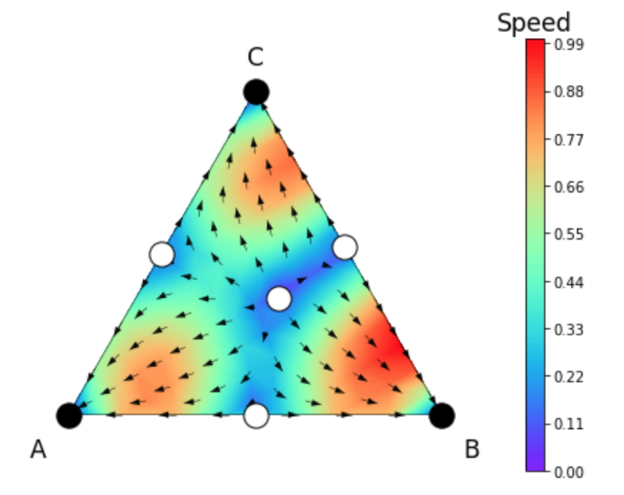
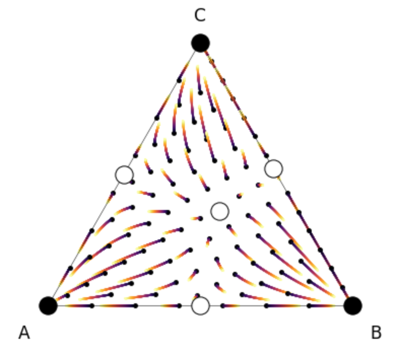
Another example of a 2-player meta-game payoff table of 3 strategies is in Table 5 with its corresponding directional field as shown in Fig. 4 and its trajectory plot in Fig. 5, where the white circles denote unstable equilibria (saddle points) and black solid circles denote globally stable equilibria.

G Proof of Theorem 4

Theorem 6.

For a Normal Form Game with $p$ players, and each player $i$ chooses a strategy $\pi^{i}$ from a set of strategies $S^{i}=\{\pi^{i}_{1},...,\pi^{i}_{k}\}$ and receives a risk averse payoff $h^{i}(\pi^{1},...,\pi^{p}):S^{1}\times...\times S^{p}\rightarrow{\mathbb{R}}$ satisfying Assumption G.4. If $\mathbf{x}$ is a Nash Equilibrium for the game $\hat{h}^{i}(\pi^{1},...,\pi^{p})$, then it is a $2\epsilon$-Nash equilibrium for the game $h^{i}(\pi^{1},...,\pi^{p})$ with probability $1-\delta$ if we play the game for $n$ times, where

$$n\geq\max\left\{-\frac{8R^{2}}{\epsilon^{2}}\log\left[\frac{1}{4}\left(1-(1-\delta)^{\frac{1}{|S^{1}|\times...\times|S^{p}|\times p}}\right)\right],\right.\left.\frac{64\beta^{2}\omega^{2}\cdot\Gamma(2)}{\epsilon^{2}\left[1-(1-\delta)^{\frac{1}{|S^{1}|\times...\times|S^{p}|\times p}}\right]}\right\}$$ (97)

Assumption G.4.

The stochastic return $h$ (for each player and each strategy) for each simulation has a sub-Gaussian tail. i,e, there exists $\omega>0$ s.t.

$$\expectation\left[exp\left(c\cdot(h-\expectation[h])\right)\right] \leq exp\left(\frac{\omega^{2}c^{2}}{2}\right)\qquad\forall c\in{\mathbb{R}}$$ (98)

And we also select $R>0$ s.t. $h\in[-R,R]$ almost surely.

Proof.

Note that we have the following relation:

$$\mathbb{E}_{\pi\sim\mathbf{x}}\left[h^{i}(\pi)\right]=\mathbb{E}_{\pi\sim\mathbf{x}}\left[\hat{h}^{i}(\pi)\right]+\mathbb{E}_{\pi\sim\mathbf{x}}\left[h^{i}(\pi)-\hat{h}^{i}(\pi)\right]$$ (99)

Then

$$\mathbb{E}_{\pi^{-i}\sim\mathbf{x}^{-i}}\left[h^{i}(\pi^{i},\mathbf{\pi}^{-i})\right]=\mathbb{E}_{\pi^{-i}\sim\mathbf{x}^{-i}}\left[\hat{h}^{i}(\pi^{i},\mathbf{\pi}^{-i})\right]+\mathbb{E}_{\pi^{-i}\sim\mathbf{x}^{-i}}\left[h^{i}(\pi^{i},\mathbf{\pi}^{-i})-\hat{h}^{i}(\pi^{i},\mathbf{\pi}^{-i})\right]$$ (100)

$$\underset{\pi^{i}}{\max}~\mathbb{E}_{\pi^{-i}\sim\mathbf{x}^{-i}}\left[h^{i}(\pi^{i},\mathbf{\pi}^{-i})\right]\leq\underset{\pi^{i}}{\max}~\mathbb{E}_{\pi^{-i}\sim\mathbf{x}^{-i}}\left[\hat{h}^{i}(\pi^{i},\mathbf{\pi}^{-i})\right]+\underset{\pi^{i}}{\max}~\mathbb{E}_{\pi^{-i}\sim\mathbf{x}^{-i}}\left[h^{i}(\pi^{i},\mathbf{\pi}^{-i})-\hat{h}^{i}(\pi^{i},\mathbf{\pi}^{-i})\right]$$ (101)

Hence,

$$\underset{\pi^{i}}{\max}~\mathbb{E}_{\pi^{-i}\sim\mathbf{x}^{-i}}\left[h^{i}(\pi^{i},\mathbf{\pi}^{-i})\right]-\mathbb{E}_{\pi\sim\mathbf{x}}\left[h^{i}(\pi)\right]$$ (102)

$$\leq \underbrace{\underset{\pi^{i}}{\max}\;\mathbb{E}_{\pi^{-i}\sim\mathbf{x}^{-i}}\left[\hat{h}^{i}(\pi^{i},\mathbf{\pi}^{-i})\right]-\mathbb{E}_{\pi\sim\mathbf{x}}\left[\hat{h}^{i}(\pi)\right]}_{=0\text{ since }\textbf{x}\text{ is a Nash Equilibrium for }\hat{h}^{i}}+\underbrace{\underset{\pi^{i}}{\max}\;\mathbb{E}_{\pi^{-i}\sim\mathbf{x}^{-i}}\left[h^{i}(\pi^{i},\mathbf{\pi}^{-i})-\hat{h}^{i}(\pi^{i},\mathbf{\pi}^{-i})\right]}_{\leq\epsilon}+\underbrace{\mathbb{E}_{\pi\sim\mathbf{x}}\left[\hat{h}^{i}(\pi)-h^{i}(\pi)\right]}_{\leq\epsilon}$$ (103)

Hence, if we can control the difference between $|h^{i}(\pi)-\hat{h}^{i}(\pi)|$ uniformly over players and actions, then an equilibrium for the empirical game is almost an equilibrium for the game defined by the reward function. Hence the question is how many samples $n$ do we need to assess that a Nash equilibrium for $\hat{h}$ is a $2\epsilon$-Nash equilibrium for $h$ for a fixed confidence $\delta$ and a fixed $\epsilon$.

In the following, in short, we fix player $i$ and the joint strategy $\pi=(\pi^{1},...,\pi^{p})$ for $p$ players and and in short, denote $h^{i}=h^{i}(\pi)$, $\hat{h}^{i}=\hat{h}^{i}(\pi)$. By Hoeffding inequality,

$$\mathbb{P}\left[\left|\bar{R^{i}}-\mathbb{E}[R^{i}]\right|\geq\frac{\epsilon}{2}\right]\leq 2\cdot exp\left(-\frac{\epsilon^{2}n}{8R^{2}}\right)$$ (104)

Now, it remains to give a batch scenario for the unbiased estimator of variance penalty term. Denote $V^{2}_{n}=\frac{1}{n-1}\sum_{j=1}^{n}\left(R^{i}_{j}-\bar{R^{i}}\right)^{2}$, then $\mathbb{E}[V^{2}_{n}]=\mathbb{V}ar[R^{i}]=\sigma^{2}$, i.e., it’s an unbiased estimator of the game variance. We first compute the variance of $V^{2}_{n}$.

Let $Z^{i}_{j}=R^{i}_{j}-\expectation[R^{i}]$, then $\expectation[Z^{i}]=0$ and $Z^{i}_{1},...Z^{i}_{n}$ are independent. Then we have

$$V^{2}_{n}=\mathbb{V}ar[R^{i}]=\mathbb{V}ar[Z^{i}].$$ (105)

$$\mathbb{V}ar[V^{2}_{n}]=\mathbb{E}[V^{4}_{n}]-(\mathbb{E}[V^{2}_{n}])^{2}$$ (106)

$$=\expectation\left[\frac{n^{2}(\sum_{j=1}^{n}(Z_{j}^{i})^{2})^{2}-2n(\sum_{j=1}^{n}(Z_{j}^{i})^{2})(\sum_{j=1}^{n}Z_{j}^{i})^{2}+(\sum_{j=1}^{n}Z_{j}^{i})^{4}}{n^{2}(n-1)^{2}}\right]-\sigma^{4}$$ (107)

$$=\frac{n^{2}\expectation\left[\left(\sum_{j=1}^{n}(Z_{j}^{i})^{2}\right)^{2}\right]-2n\expectation\left[\left(\sum_{j=1}^{n}(Z_{j}^{i})^{2}\right)\left(\sum_{j=1}^{n}Z_{j}^{i}\right)^{2}\right]+\expectation\left[\left(\sum_{j=1}^{n}Z_{j}^{i}\right)^{4}\right]}{n^{2}(n-1)^{2}}-\sigma^{4}$$ (108)

Since $Z_{1}^{i},...,Z_{n}^{i}$ are independent, then we have that for distinct $j,k,m$,

$$\expectation[Z^{i}_{j}Z^{i}_{k}]=0;\quad\expectation[(Z^{i}_{j})^{3}Z^{i}_{k}]=0;\quad\expectation[(Z^{i}_{j})^{2}Z^{i}_{k}Z^{i}_{m}]=0.$$ (109)

And we denote

$$\expectation[(Z^{i}_{j})^{2}(Z^{i}_{k})^{2}]=\mu_{2}^{2}=\sigma^{4};\quad\expectation[(Z^{i}_{j})^{4}]=\mu_{4}.$$ (110)

Then, with algebraic manipulations, we can simplify Eq. 106 as:

$$\mathbb{V}ar[V_{n}^{2}] =\frac{n^{2}\left(n\mu_{4}+n(n-1)\mu_{2}^{2}\right)-2n(n\mu_{4}+n(n-1)\mu_{2}^{2})+n\mu_{4}+3n(n-1)\mu_{2}^{2}}{n^{2}(n-1)^{2}}-\sigma^{4}$$ (111)

$$=\frac{(n-1)\mu_{4}+(n^{2}-2n+3)\sigma^{4}}{n(n-1)}-\sigma^{4}$$ (112)

$$=\frac{\mu_{4}}{n}-\frac{\sigma^{4}(n-3)}{n(n-1)}.$$ (113)

By Chebyshev’s inequality,

$$\mathbb{P}\left[\left|V_{n}^{2}-\mathbb{V}ar[R^{i}]\right|\geq\frac{\epsilon}{2\beta}\right] \leq\frac{\mathbb{V}ar[V_{n}^{2}]}{(\frac{\epsilon}{2\beta})^{2}}$$ (114)

$$\leq\frac{4\beta^{2}\left(\frac{\mu_{4}}{n}-\frac{\sigma^{4}(n-3)}{n(n-1)}\right)}{\epsilon^{2}}$$ (115)

By Assumption G.4,

$$\mu_{4}\leq 16\omega^{2}\cdot\Gamma(2)$$ (116)

By triangle inequality,

$${\mathbb{P}}\left[\left|h^{i}-\hat{h}^{i}\right|\geq\epsilon\right] \leq{\mathbb{P}}\left[\left|\expectation[R^{i}]-\bar{R}^{i}\right|+\beta\cdot\left|V_{n}^{2}-\mathbb{V}ar[R^{i}]\right|\geq\epsilon\right]$$ (117)

$$\leq{\mathbb{P}}\left[\left|\expectation[R^{i}]-\bar{R}^{i}\right|\geq\frac{\epsilon}{2}\;or\;\beta\cdot\left|V_{n}^{2}-\mathbb{V}ar[R^{i}]\right|\geq\frac{\epsilon}{2}\right]$$ (118)

$$\leq{\mathbb{P}}\left[\left|\expectation[R^{i}]-\bar{R}^{i}\right|\geq\frac{\epsilon}{2}\right]+{\mathbb{P}}\left[\left|V_{n}^{2}-\mathbb{V}ar[R^{i}]\right|\geq\frac{\epsilon}{2\beta}\right]$$ (119)

$$\leq 2\cdot exp\left(-\frac{\epsilon^{2}n}{8R^{2}}\right)+\frac{4\beta^{2}\left(\frac{16\omega^{2}\cdot\Gamma(2)}{n}-\frac{\sigma^{4}(n-3)}{n(n-1)}\right)}{\epsilon^{2}}$$ (120)

$$\leq 2\cdot exp\left(-\frac{\epsilon^{2}n}{8R^{2}}\right)+\frac{64\beta^{2}\omega^{2}\cdot\Gamma(2)}{n\epsilon^{2}}$$ (121)

$$=f(n,\epsilon).$$ (122)

Hence, for per joint strategies $\pi$ and per player $i$, we have the following bound :

$${\mathbb{P}}\left[\underset{\pi,i}{\sup}\left|h^{i}(\pi)-\hat{h}^{i}(\pi)\right|<\epsilon\right]\geq\left(1-f(n,\epsilon)\right)^{|S^{1}|\times...\times|S^{p}|\times p}$$ (123)

Hence, for

$$n\geq\max\left\{-\frac{8R^{2}}{\epsilon^{2}}\log\left[\frac{1}{4}\left(1-(1-\delta)^{\frac{1}{|S^{1}|\times...\times|S^{p}|\times p}}\right)\right]\;;\;\frac{64\beta^{2}\omega^{2}\cdot\Gamma(2)}{\epsilon^{2}\left[1-(1-\delta)^{\frac{1}{|S^{1}|\times...\times|S^{p}|\times p}}\right]}\right\}$$ (124)

we have ${\mathbb{P}}\left[\underset{\pi,i}{\sup}\left|h^{i}(\pi)-\hat{h}^{i}(\pi)\right|<\epsilon\right]\geq 1-\delta$.

Plugging the result into Eq. 102, we have

$$\underset{\pi^{i}}{\max}~\mathbb{E}_{\pi^{-i}\sim\mathbf{x}^{-i}}\left[h^{i}(\pi^{i},\mathbf{\pi}^{-i})\right]-\mathbb{E}_{\pi\sim\mathbf{x}}\left[h^{i}(\pi)\right]\leq 2\epsilon$$ (125)

∎

References

- Anschel et al. (2017) Anschel, O., Baram, N., and Shimkin, N. Averaged-dqn: Variance reduction and stabilization for deep reinforcement learning. In International Conference on Machine Learning, pp. 176–185. PMLR, 2017.
- Bagherzadeh et al. (2020) Bagherzadeh, M., Kahani, N., and Briand, L. Reinforcement learning for test case prioritization. arXiv preprint arXiv:2011.01834, 2020.
- Balch et al. (2019) Balch, T. H., Mahfouz, M., Lockhart, J., Hybinette, M., and Byrd, D. How to evaluate trading strategies: Single agent market replay or multiple agent interactive simulation? arXiv preprint arXiv:1906.12010, 2019.
- Bellemare et al. (2020) Bellemare, M. G., Candido, S., Castro, P. S., Gong, J., Machado, M. C., Moitra, S., Ponda, S. S., and Wang, Z. Autonomous navigation of stratospheric balloons using reinforcement learning. Nature, 588(7836):77–82, 2020.
- Berner et al. (2019) Berner, C., Brockman, G., Chan, B., Cheung, V., Debiak, P., Dennison, C., Farhi, D., Fischer, Q., Hashme, S., Hesse, C., et al. Dota 2 with large scale deep reinforcement learning. arXiv preprint arXiv:1912.06680, 2019.
- Bertsekas (2009) Bertsekas, D. P. Neuro-dynamic programmingNeuro-Dynamic Programming, pp. 2555–2560. Springer US, Boston, MA, 2009. ISBN 978-0-387-74759-0. doi: 10.1007/978-0-387-74759-0_440. URL https://doi.org/10.1007/978-0-387-74759-0_440.
- Bloembergen et al. (2015) Bloembergen, D., Hennes, D., McBurney, P., and Tuyls, K. Trading in markets with noisy information: An evolutionary analysis. Connection Science, 27(3):253–268, 2015.
- Bowling (2000) Bowling, M. Convergence problems of general-sum multiagent reinforcement learning. In ICML, pp. 89–94, 2000.
- Bowling & Veloso (2002) Bowling, M. and Veloso, M. Multiagent learning using a variable learning rate. Artificial Intelligence, 136(2):215–250, 2002.
- Buldygin & Kozachenko (1980) Buldygin, V. V. and Kozachenko, Y. V. Sub-gaussian random variables. Ukrainian Mathematical Journal, 32(6):483–489, 1980. doi: 10.1007/BF01087176.
- Byrd et al. (2019) Byrd, D., Hybinette, M., and Balch, T. H. Abides: Towards high-fidelity market simulation for ai research. arXiv preprint arXiv:1904.12066, 2019.
- Di Castro et al. (2012) Di Castro, D., Tamar, A., and Mannor, S. Policy gradients with variance related risk criteria. arXiv preprint arXiv:1206.6404, 2012.
- Filar & Vrieze (1997) Filar, J. and Vrieze, K. Competitive Markov Decision Processes. Springer, 1997.
- Garcıa & Fernández (2015) Garcıa, J. and Fernández, F. A comprehensive survey on safe reinforcement learning. Journal of Machine Learning Research, 16(1):1437–1480, 2015.
- Henderson et al. (2018) Henderson, P., Islam, R., Bachman, P., Pineau, J., Precup, D., and Meger, D. Deep reinforcement learning that matters. In Proceedings of the AAAI Conference on Artificial Intelligence, volume 32, 2018.
- Hu & Wellman (1998) Hu, J. and Wellman, M. P. Multiagent reinforcement learning: Theoretical framework and an algorithm. In Proceedings of the Fifteenth International Conference on Machine Learning, ICML ’98, pp. 242–250, San Francisco, CA, USA, 1998. Morgan Kaufmann Publishers Inc. ISBN 1558605568.
- Johnson & Zhang (2013) Johnson, R. and Zhang, T. Accelerating stochastic gradient descent using predictive variance reduction. In Burges, C. J. C., Bottou, L., Welling, M., Ghahramani, Z., and Weinberger, K. Q. (eds.), Advances in Neural Information Processing Systems, volume 26. Curran Associates, Inc., 2013.
- Li (2017) Li, Y. Deep reinforcement learning: An overview. arXiv preprint arXiv:1701.07274, 2017.
- Li et al. (2009) Li, Y., Szepesvari, C., and Schuurmans, D. Learning exercise policies for american options. In Artificial Intelligence and Statistics, pp. 352–359. PMLR, 2009.
- Littman (2001) Littman, M. L. Value-function reinforcement learning in markov games. Cognitive systems research, 2(1):55–66, 2001.
- Mihatsch & Neuneier (2002) Mihatsch, O. and Neuneier, R. Risk-sensitive reinforcement learning. Machine learning, 49(2):267–290, 2002.
- Mirhoseini et al. (2020) Mirhoseini, A., Goldie, A., Yazgan, M., Jiang, J., Songhori, E., Wang, S., Lee, Y.-J., Johnson, E., Pathak, O., Bae, S., et al. Chip placement with deep reinforcement learning. arXiv preprint arXiv:2004.10746, 2020.
- Morimoto & Doya (2005) Morimoto, J. and Doya, K. Robust reinforcement learning. Neural computation, 17(2):335–359, 2005.
- Ning et al. (2018) Ning, B., Lin, F. H. T., and Jaimungal, S. Double deep q-learning for optimal execution. arXiv preprint arXiv:1812.06600, 2018.
- Pan et al. (2019) Pan, X., Seita, D., Gao, Y., and Canny, J. Risk averse robust adversarial reinforcement learning. In 2019 International Conference on Robotics and Automation (ICRA), pp. 8522–8528. IEEE, 2019.
- Pinto et al. (2017) Pinto, L., Davidson, J., Sukthankar, R., and Gupta, A. Robust adversarial reinforcement learning. In International Conference on Machine Learning, pp. 2817–2826. PMLR, 2017.
- Sharpe (1994) Sharpe, W. F. The sharpe ratio. Journal of portfolio management, 21(1):49–58, 1994.
- Shen et al. (2014) Shen, Y., Tobia, M. J., Sommer, T., and Obermayer, K. Risk-sensitive reinforcement learning. Neural computation, 26(7):1298–1328, 2014.
- Spooner et al. (2018) Spooner, T., Fearnley, J., Savani, R., and Koukorinis, A. Market making via reinforcement learning. arXiv preprint arXiv:1804.04216, 2018.
- Szepesvári & Littman (1999) Szepesvári, C. and Littman, M. A unified analysis of value-function-based reinforcement-learning algorithms. Neural computation, 11:2017–59, 12 1999. doi: 10.1162/089976699300016070.
- Théate & Ernst (2021) Théate, T. and Ernst, D. An application of deep reinforcement learning to algorithmic trading. Expert Systems with Applications, 173:114632, 2021.
- Tobia et al. (2013) Tobia, M., Guo, R., Schwarze, U., Böhmer, W., Gläscher, J., Finckh, B., Marschner, A., Büchel, C., Obermayer, K., and Sommer, T. Neural systems for choice and valuation with counterfactual learning signals. NeuroImage, 89, 12 2013. doi: 10.1016/j.neuroimage.2013.11.051.
- Tuyls et al. (2020) Tuyls, K., Perolat, J., Lanctot, M., Hughes, E., Everett, R., Leibo, J. Z., Szepesvári, C., and Graepel, T. Bounds and dynamics for empirical game theoretic analysis. Autonomous Agents and Multi-Agent Systems, 34(1):1–30, 2020.
- Wainwright (2019) Wainwright, M. J. Variance-reduced -learning is minimax optimal. arXiv preprint arXiv:1906.04697, 2019.
- Walsh et al. (2002) Walsh, W. E., Das, R., Tesauro, G., and Kephart, J. O. Analyzing complex strategic interactions in multi-agent systems. In AAAI-02 Workshop on Game-Theoretic and Decision-Theoretic Agents, pp. 109–118, 2002.
- Weibull (1997) Weibull, J. W. Evolutionary game theory. MIT press, 1997.
- Weinberg & Rosenschein (2004) Weinberg, M. and Rosenschein, J. S. Best-response multiagent learning in non-stationary environments. In Proceedings of the Third International Joint Conference on Autonomous Agents and Multiagent Systems-Volume 2, pp. 506–513, 2004.
- Wellman (2006) Wellman, M. P. Methods for empirical game-theoretic analysis. In AAAI, pp. 1552–1556, 2006.