AI-Based Secure NOMA and Cognitive Radio enabled Green Communications: Channel State Information and Battery Value Uncertainties

Abstract

In this paper, the security-aware robust resource allocation in energy harvesting cognitive radio networks is considered with cooperation between two transmitters while there are uncertainties in channel gains and battery energy value. To be specific, the primary access point harvests energy from the green resource and uses time switching protocol to send the energy and data towards the secondary access point (SAP). Using power-domain non-orthogonal multiple access technique, the SAP helps the primary network to improve the security of data transmission by using the frequency band of the primary network. In this regard, we introduce the problem of maximizing the proportional-fair energy efficiency (PFEE) considering uncertainty in the channel gains and battery energy value subject to the practical constraints. Moreover, the channel gain of the eavesdropper is assumed to be unknown. Employing the decentralized partially observable Markov decision process, we investigate the solution of the corresponding resource allocation problem. We exploit multi-agent with single reward deep deterministic policy gradient (MASRDDPG) and recurrent deterministic policy gradient (RDPG) methods. These methods are compared with the state-of-the-art ones like multi-agent and single-agent DDPG. Simulation results show that both MASRDDPG and RDPG methods, outperform the state-of-the-art methods by providing more PFEE to the network.

I Introduction

I-A Background

Cognitive radio (CR) is a promising way to improve the spectrum efficiency due to the ability of the system to reassign unoccupied frequencies [1]. In the CR network, there are two kinds of network nodes, a primary that is known as the owner of the spectrum and a secondary which uses the frequency based on different policies. These policies can be divided into three categories as interweave, underlay, and overlay [2]. In the interweave and underlay CR network, the secondary is given permission to use the spectrum when there is vacancy in frequency band and an acceptable interference to the primary receiver, respectively. Moreover, in the overlay case, the secondary network cooperates with the primary in order to improve the primary throughput. The overlay case is also called as cooperative cognitive which is widely studied in [3, 4].
Wireless powered communication networks (WPCNs) are considered often which are promising techniques to provide a stable energy resource in energy limited devices [5, 6]. Recently, this technique is combined with CR networks as cognitive wireless powered communication networks (CWPCNs) [2, 7, 8]. There are two popular energy harvesting (EH) techniques which are used in CWPCNs, time-switching (TS) and power-splitting (PS) schemes [9, 10].
In order to prolong the network lifespan in energy-limited devices and decrease the harmful effect of energy production on the environment, energy efficient (EE) resource allocation is introduced in [11, 12]. In addition, the combination of the EE resource allocation problem and the CWPCNs is adopted in [13, 14] which improves the energy consumption at power restrictive cognitive transmitters. The popular EE resource allocation problems can be divided into four main categories such as global EE, proportional fair EE (PFEE), max-min fair EE (MMFEE), and harmonic fair EE (HFEE) methods [15]. In the global EE, the ratio of rate to energy is maximized. Moreover, in PFEE, MMFEE, and HFEE, the objectives are maximizing the logarithm of EE, maximizing the minimum value of EE, and minimizing the reverse of EE, respectively.
The uncertainty in the telecommunication system is inevitable. The assumption of perfect information about environment or the battery value in devices due to the stochastic nature of wireless channel, delays or failure of circuit of devices mostly is impossible. The unavailability or imperfection of these kinds of information leads to performance degradation of the network and subsequently, the network efficiency decreases. The uncertainty may exist in any section of the communication network like channel gain [16, 17], locations of devices [18], and demand and capacity of available resources [19].
Moreover, power domain non-orthogonal multiple access (PD-NOMA) is one of the main candidates for improving the next generation of cellular network. PD-NOMA can easily enhance throughput due to high spectral efficiency (SE). In contrast to orthogonal multiple access (OMA) that only assigns one resource block to each user, the main idea of PD-NOMA is to exploit one orthogonal channel resource block for more than one user to improve SE [20, 21].

I-B Literature Review

Recently, there have been many works which address the challenges of using the EH in wireless communications. We categorize the the aforementioned studies in the following groups:

• EH and EE: The joint EH and EE maximization problem is investigated in [22, 23, 24, 10, 13]. The authors in [22] try to maximize EE of D2D link by considering the QoS of users and the causality constraint of D2D links. [23] proposes an EE maximization problem in heterogeneous networks based on simultaneous wireless information and power transfer (SWIPT) and NOMA. In this paper, the power allocation and sub-channel matching resource allocation problem subject to the interference threshold is investigated. Moreover, the devices convert the received signal of other BSs into energy. [24] investigates EE maximization problem in SWIPT AF relay networks. The authors formulate their proposed problem with the goal of optimizing the source and relays total transmit powers, joint sub-carrier and user assignment, and relay selection and TS coefficient determination subject to total transmit power budget of source and energy casualty constraints of relays. The combination of robust EE and EH in heterogeneous networks where each femtocell adopts SWIPT is considered in [10]. The authors propose the EE maximization problem subject to outage probability of macrocell users (MUs) to optimize transmit power allocation and PS factor.

• Secrecy and EH: [25, 26, 2, 27] consider the combination of secrecy and EH. The physical security in SWIPT AF relay network is considered in [25], while the imperfect channel gain between relays and the eavesdroppers is modeled by random CSI errors. The objective is secure data transmission with constraints on relays transmit powers and the eavesdropper signal to interference plus noise ratio (SINR). Moreover, there is no direct link between the transmitter and the receiver, and the eavesdropper can only listen to the signals that are transmitted by relays. The authors of [26] consider NOMA technique and nonlinear EH model to maximize the secrecy energy efficiency. In [2], the CR network is considered to maximize the secondary users (SUs) ergodic rate. Furthermore, the SUs, which are not supposed to transmit data, are considered to transmit artificial noise toward the eavesdroppers.

• Artificial Intelligence and EH: Artificial Intelligence (AI)-based EH problem with a cooperating node between source-destination pairs is proposed in [28]. In this work the relay decides which link at each time slot has permission to transmit under the EH constraint. The authors of [29] consider the effective energy management in wireless sensor network by utilizing the Deep Deterministic Policy Gradient (DDPG) reinforcement learning method. In [30], the problem of long term throughput maximization in point to point communication is solved by using the DDPG method.

• AI and uncertainty: [31] studies the effect of uncertainty in channel gains in wireless secure communication system with coexistence of intelligent reflecting surface (IRS). The authors propose the post decision state (PDS) and prioritized experience replay (PER) techniques to improve the learning efficiency as well as performance of secure communication. However, they consider that the BSs know CSI of the eavesdropper which is not applicable in the real environment.

Various optimization problems with different technologies and restrictions have been widely studied in the EH secure wireless communication network. Most of these works use an iterative algorithm to find the optimal or sub-optimal solutions. These solutions mostly involve high computational complexity which can not be deployed in sensors or small nodes. Moreover, due to the dynamic behavior of wireless channel conditions, these algorithms have to be updated in a very short time duration which is impractical in real environment.

The problems of uncertainty in the channel gain and other parameters of the network are still the bottleneck in wireless communication. This situation gets worse when an eavesdropper with unknown channel gain enters into the system. By considering these issues, machine learning techniques can be considered as a great way to learn the condition of the network and solve the problem in a timely manner. The only recent paper which uses machine learning algorithm to deal with the channel gain uncertainty in cognitive radio network is [31]. The authors adopt single agent reinforcement learning method in which the state of the environment is fully observable to the agent, even the eavesdropper channel gain, to decide the appropriate action. On the other hand, considering the uncertainty constraints as probabilistic expressions provides more robustness to the solution which is neglected in their formulation.
Motivated by these considerations, in this paper we formulate the EH-enabled CR network with Time Switching PD-NOMA (TS-NOMA) technique, as a multi agent partially observable Markov decision process (POMDP) in an uncertain environment, considering the existence of an eavesdropper. The partially observability means that the agent does not have full state information of the channel gains of some devices, i.e., the eavesdropper, and the uncertainty means the agent knows the battery energy level and channel gains with bounded errors. We consider three different formulations for the uncertainty in our environment as the worst case, probabilistic, and Bernstein approximation, and formulate our problem based on these three schemes. Then we utilize two deep reinforcement learning methods which are suitable for partially observable and uncertain environment as 1) multi agent deep deterministic policy gradient with single reward (MASRDDPG) and 2) deep recurrent deterministic policy gradient (RDPG) as a solution for our problem.

I-C Contribution

To the best of the authors’ knowledge, considering the CR EH-enabled with uncertain conditions and partially observable environment to overcome the uncertainty of the information has not been done by previous AI-based researches. Accordingly, the main contributions of this paper are summarized as follows:

• We investigate PD-NOMA cooperative cognitive TS based EH system with the existence of an eavesdropper, and the uncertainty of channel gains, the amount of harvesting energy, and the battery energy level. To this end, we consider that there is one primary access point (PAP) that sends information to the primary user equipment (PUE). However, due to poor channel condition, the secondary access point (SAP) which harvests energy by the TS techniques, helps to forward data of the PUE to achieve opportunity of transmitting its own information. The eavesdropper tries to listen to the transmitted data in the network.

• We formulate EE optimization problem in which the objective is to maximize the secure PFEE by finding transmit powers and the TS factor in the partially observable environment with uncertain values, while considering battery energy constraints, the QoS requirement of the PUE, energy causality limitations, and the total transmit power budget.

• By considering uncertainties in the channel gains and the battery values, we adopt the worst case, the probabilistic, and the Bernstein approximation approaches for the uncertainties and reformulate the resource allocation problem. Then we utilize RDPG method, which is suitable for the partially observable and uncertain environment. In addition, by considering different objectives for the PAP and the SAP along with their common objective to serving the PUE, we adopt the MASRDDPG method to cope with the single and shared objectives besides the partially observability.

• By conducting numerical simulations, when considering the single reward along with shared reward for multi agent method, the MASRDDPG outperforms by 5.6%, 22.7%, and 31.8% compared to RDPG, MADDPG, and DDPG methods, respectively, from the average secrecy rate point of view. On the other hand, by the expense of time complexity, using recurrent neural network (RNN) to support the uncertainty and partially observability in the environment, the RDPG method outperforms the MADDPG and DDPG by 16.4% and 25.2%, respectively, from the average secrecy rate point of view.

I-D Structure

The rest of this paper is organized as follows. In Section II, we present our proposed the TS-NOMA system model with cooperative transmission and the EH capability. In Section III, we propose a navel solution and algorithm to find an optimal energy consumption of network. In Section IV, the simulation results are provided. Finally, Section V concludes the paper.

II System model and problem formulation

Fig. 1: Network model for the EH secure CR network with PD-NOMA technique, where the PAP harvests energy from renewable source and the SAP absorbs energy based on time switching technique and use PD-NOMA protocol.

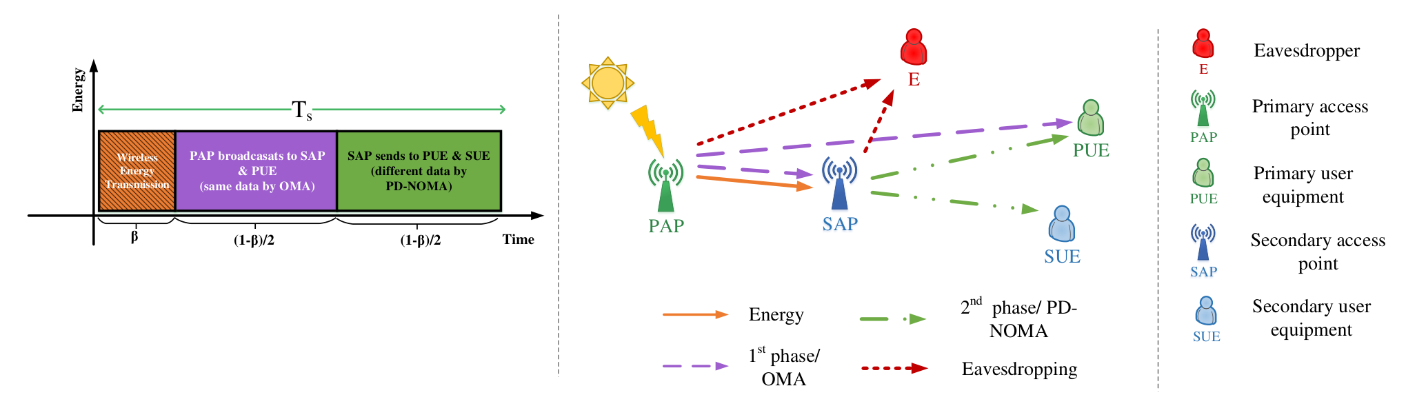
We consider an EH downlink cooperative secure PD-NOMA network with primary transmission which works as an overlay network, secondary transmission that works as an underlay network, and an eavesdropper. The architecture of the system model is illustrated in Fig. 1.

The primary network consists of a PAP as a transmitter equipped with a finite capacity battery with the capability of harvesting energy from green energies such as solar energy and wind power and storing surplus of energy in the battery and a PUE which is served by the PAP. The secondary network underlays the primary one and uses the bandwidth of the primary network with agreement on helping to forward the PAP data toward its receiver. The secondary network consists of one SAP as a transmitter and a secondary user equipment (SUE) as a receiver. The SAP harvests energy from the RF signals transmitted by the PAP in the TS mode and uses this energy to decode-and-forward the signal of the PAP besides sending its own data. The SAP is equipped with a finite battery to save surplus energy units for future usage. The malicious user in this network tries to eavesdrop data of all transmitters through the direct link and the cooperative link. Moreover, each node is equipped with a single antenna.

Let $T_{D}$ be the number of time slots over which the communication system is studied and the length of each time slot is $T_{s}$. Moreover, we assume that the CSI remains constant during each time slot $t_{d}$ and changes independently from one time slot to other time slot. As shown in Fig.1, OMA and PD-NOMA techniques are adopting at the PAP and the SAP, respectively, for data transmission. In the first phase, the PAP sends energy with power $p_{pp}(t_{d})$ with duration $\beta\in[0,1]$ to the SAP. $\beta=1$ means that there is no time for data transmission and $\beta=0$ means that the system considers that there is no need for energy transmission. In this phase, the SAP harvests energy from the RF signal and employs it to forward the PAP data to the PUE, as well as its own information to the SUE. The harvested energy at the SAP can be expressed as follows:

$$E_{s}(t_{d}) =T_{s}\beta\eta_{2,s}p_{pp}(t_{d})h_{\text{PAP}\rightarrow\text{SAP}}(t_{d}),$$ (1)

where $h_{\text{PAP}\rightarrow\text{SAP}}(t_{d})$ is the channel gain from the PAP to the PUE at time slot $t_{d}$ and $\eta_{2,s}\in(0,1]$ is the energy conversion efficiency at the SAP. During the second phase, the PAP broadcasts its message based on OMA technique. The signal to noise ratio (SNR) at the PUE is calculated as follows:

$$\gamma_{\text{PAP}\rightarrow\text{PUE}}^{\text{}}(t_{d})=\frac{p_{pp}(t_{d})h_{\text{PAP}\rightarrow\text{PUE}}(t_{d})}{\sigma^{2}_{pp}},$$ (2)

where $\sigma^{2}_{pp}$ is the variance of additive Gaussian white noise (AWGN) at the PUE. The received data rate in (bit/s/Hz) at the SAP is given by

$$r_{\text{PAP}\rightarrow\text{SAP}}(t_{d}) =\frac{(1-\beta)}{2}\log_{2}\Big(1+\frac{p_{pp}(t_{d})h_{\text{PAP}\rightarrow\text{SAP}}(t_{d})}{\sigma_{ps}^{2}}\Big),$$ (3)

where $h_{\text{PAP}\rightarrow\text{SAP}}(t_{d})$ is the channel gain from the PAP to the SAP and $\sigma^{2}_{ps}$ is the variance of AWGN at the SAP. The SNR at the eavesdropper can be formulated as

$$\gamma_{\text{PAP}\rightarrow E}(t_{d})=\frac{p_{pp}(t_{d})h_{\text{PAP}\rightarrow E}(t_{d})}{\sigma_{pe}^{2}},$$ (4)

where $h_{\text{PAP}\rightarrow E}(t_{d})$ is channel gain from the PAP to the eavesdropper and $\sigma_{pe}^{2}$ is the variance of AWGN at the eavesdropper side. In the third phase, the SAP decodes the received signal from the PAP and by utilizing PD-NOMA technique, it simultaneously sends the decoded signal and its own message towards the PUE and the SUE, respectively.

Based on the relation between the channel gain from the SAP to the PUE, i.e., $h_{\text{SAP}\rightarrow\text{PUE}}(t_{d})$, and the channel gain from the SAP to the SUE, i.e., $h_{\text{SAP}\rightarrow\text{SUE}}(t_{d})$, there are two scenarios. In the first scenario, if $h_{\text{SAP}\rightarrow\text{PUE}}(t_{d})\geq h_{\text{SAP}\rightarrow\text{SUE}}(t_{d})$, the successive interference cancellation (SIC) is implemented at the PUE, and the SUE suffers from interference. Hence, the SNR at the PUE after removing the interference can be written as follows:

$$\gamma_{\text{SAP}\rightarrow\text{PUE}}^{\text{SCN I}}(t_{d})=\frac{p_{sp}(t_{d})h_{\text{SAP}\rightarrow\text{PUE}}(t_{d})}{\sigma_{sp}^{2}},$$ (5)

where $\sigma^{2}_{sp}$ is the variance of AWGN, then the SNR at the SUE can be shown as follows:

$$\gamma_{\text{SAP}\rightarrow\text{SUE}}^{\text{SCN I}}(t_{d})=\frac{p_{ss}(t_{d})h_{\text{SAP}\rightarrow\text{SUE}}(t_{d})}{p_{sp}(t_{d})h_{\text{SAP}\rightarrow\text{SUE}}(t_{d})+\sigma_{ss}^{2}},$$ (6)

where $\sigma^{2}_{ss}$ is the variance of AWGN. In the second scenario, if $h_{\text{SAP}\rightarrow\text{SUE}}(t_{d})>h_{\text{SAP}\rightarrow\text{PUE}}(t_{d})$, the SIC is implemented by the SUE and the PUE suffers from PD-NOMA interference. The throughput at the SUE is expressed as

$$r_{\text{SAP}\rightarrow\text{SUE}}^{\text{SCN II}}(t_{d}) =\frac{(1-\beta)}{2}\log_{2}\Big(1+\frac{p_{ss}(t_{d})h_{\text{SAP}\rightarrow\text{SUE}}(t_{d})}{\sigma_{ss}^{2}}\Big),$$ (7)

and the data rate at the PUE side can be formulated as follows:

$$r_{\text{SAP}\rightarrow\text{PUE}}^{\text{SCN II}}(t_{d})=\frac{(1-\beta)}{2}\log_{2}\Big(1+\frac{p_{sp}(t_{d})h_{\text{SAP}\rightarrow\text{PUE}}(t_{d})}{p_{ss}(t_{d})h_{{\text{SAP}\rightarrow\text{PUE}}}(t_{d})+\sigma_{sp}^{2}}\Big).$$ (8)

Here, we consider the worst case for eavesdropper where it uses strong multiuser detection techniques and can successfully cancel the interference signal from the PAP and the SAP [32, 33]. The received SNR at the eavesdropper at this phase is

$$\gamma_{\text{SAP}1\rightarrow{E}}(t_{d}) =\frac{h_{\text{SAP}\rightarrow E}(t_{d})p_{sp}(t_{d})}{\sigma_{se}^{2}}.$$ (9)

At the end of second phase, the PUE catches information from the PAP and the SAP, and decodes the received massages jointly by using the maximum ratio combining (MRC). Therefore, the data rate in (bit/s/Hz) based on the MRC in the PUE can be described as

$$r_{\text{MRC-P}}^{\text{S}}(t_{d}) =\frac{(1-\beta)}{2}\log_{2}\big(1+\gamma_{\text{PAP}\rightarrow\text{PUE}}(t_{d})+\gamma_{\text{SAP}\rightarrow\text{PUE}}^{\text{S}}(t_{d})\big),$$ (10)

where $\text{S}\in[\text{SCN I},\text{SCN II}]$.

The throughput related to the PUE’s data at the eavesdropper can be formulated as follows:

$$r_{\text{MRC-E}}(t_{d}) =\frac{1-\beta}{2}\log_{2}\big(1+\gamma_{\text{PAP}\rightarrow E}(t_{d})+\gamma_{\text{SAP}1\rightarrow{E}}(t_{d})\big).$$ (11)

The data rate in (bit/s/Hz) related to the SUE’s data at the eavesdropper can be formulated as follows:

$$r_{\text{SAP2}\rightarrow E}(t_{d}) =\frac{1-\beta}{2}\log_{2}\Big(1+\frac{p_{ss}(t_{d})h_{\text{SAP}\rightarrow E}(t_{d})}{\sigma_{ss}^{2}}\Big).$$ (12)

We suppose that the harvested energy will be stored in the battery and each transmitter only uses the stored energy in their batteries. Hence, at the beginning of time slot $t_{d}$, the remaining energy in the batteries can be formulated as

$$B_{p}(t_{d}) =\min\{B_{\max,p},B_{p}(t_{d}-1)+\eta_{1,p}E_{p}^{\text{RE}}(t_{d}-1)-T_{s}\big(\beta+\frac{(1-\beta)}{2})p_{pp}(t_{d}-1)-E_{\text{P}}^{\text{Cons}}\},$$ (13)

$$B_{s}(t_{d}) =\min\{B_{\max,s},B_{s}(t_{d}-1)+{\eta_{1,s}E_{s}(t_{d})}-T_{s}\frac{(1-\beta)}{2}\big(p_{sp}(t_{d}-1)+p_{ss}(t_{d}-1)\big)-E_{\text{S}}^{\text{Cons}}\},$$ (14)

where $B_{p}(t_{d}-1)$ and $B_{s}(t_{d}-1)$ are the energy value of batteries of the PAP and the SAP at the beginning of previous time slot, and $B_{p}(0)=B_{p,0}$ and $B_{s}(0)=B_{s,0}$. Let ${E_{p}^{\text{RE}}(t_{d})}$ denote the amount of energy received at the PAP at time slot $t_{d}$. $E_{\text{P}}^{\text{Cons}}$ and $E_{\text{S}}^{\text{Cons}}$ are the constant energy consumption for the operation of the PAP and the SAP. Moreover, $B_{\max,p}$ and $B_{\max,s}$ are the maximum capacity of batteries for the PAP and the SAP, respectively. $\eta_{1,p}\in(0,1]$ and $\eta_{1,s}\in(0,1]$ are the storage efficiencies of the PAP and the SAP. It is worth mentioning that we assume the SAP can use the harvested energy from the PAP in the same time slot since the SAP will begin to transmit if and only if the signal reception from the PAP has ended. By the way, the PAP uses the harvested energy only at the next time slot when energy units have received completely.

The total secrecy rate of the network at the end of each time slot can be formulated as follows:

$$R(t_{d}) =\Big[\min\big(r_{\text{PAP}\rightarrow\text{SAP}}(t_{d}),r_{\text{MRC-P}}^{\text{S}}(t_{d})\big)-r_{\text{MRC-E}}(t_{d})\Big]^{+}+\Big[r_{\text{SAP}\rightarrow\text{SUE}}^{\text{S}}(t_{d})-r_{\text{SAP2}\rightarrow E}(t_{d})\Big]^{+},$$ (15)

and the total energy consumption at each time slot can be computed as follows:

$$E(t_{d})=T_{s}\nu\Big(\big(\beta+\frac{(1-\beta)}{2}\big)p_{pp}(t_{d})+\frac{(1-\beta)}{2}\big(p_{sp}(t_{d})+p_{ss}(t_{d})\big)\Big)-\nu E_{s}(t_{d})+E_{c}.$$ (16)

II-A Uncertainty and Robustness

The uncertainty can be classified into two categories as aleatoric and epistemic which arise from stochastic behavior and parameter estimation, respectively [34]. The aleatoric is a statistical and random uncertainty and cannot be predicted by collecting more information and knowledge. On the other hand, the epistemic uncertainty can be modeled by using probability distribution functions and diminished through collecting more information about the uncertain system [34]. In the CR networks, we are dealing with the epistemic uncertainty, therefore it can be handled by using methods which collects previous information of the uncertain system [34]. In the following, we investigate the uncertainties about channel gains and battery energy values.

II-A1 Channel Uncertainty

Here, we suppose that the perfect CSI between the transmitters and the receivers is not available. This uncertainty comes from the disability of the network in catching the appropriate value of channel gain, due to the error in the feedback channels and/or out-date channel value [35, 34]. The uncertainty of channel gains can be represented by the summation of estimated channel value and additive error as follows:

$$h_{\text{PAP}\rightarrow\text{PUE}}(t_{d}) =\bar{h}_{\text{PAP}\rightarrow\text{PUE}}(t_{d})+\epsilon_{h_{\text{PAP}\rightarrow\text{PUE}}(t_{d})},$$ (17)

$$h_{\text{PAP}\rightarrow\text{SAP}}(t_{d}) =\bar{h}_{\text{PAP}\rightarrow\text{SAP}}(t_{d})+\epsilon_{h_{\text{PAP}\rightarrow\text{SAP}}(t_{d})},$$ (18)

$$h_{\text{SAP}\rightarrow\text{PUE}}(t_{d}) =\bar{h}_{\text{SAP}\rightarrow\text{PUE}}(t_{d})+\epsilon_{h_{\text{SAP}\rightarrow\text{PUE}}(t_{d})},$$ (19)

$$h_{\text{SAP}\rightarrow\text{SUE}}(t_{d}) =\bar{h}_{\text{SAP}\rightarrow\text{SUE}}(t_{d})+\epsilon_{h_{\text{SAP}\rightarrow\text{SUE}}(t_{d})},$$ (20)

where $\bar{h}_{[\cdot]}$ and $\epsilon_{[\cdot]}$ are the estimated and error values of channel gain, respectively, and $h_{[\cdot]}(t_{d})$ is the exact values of the channels. Moreover, we define the uncertainty region for each channel gain as the distance from the actual and the estimated values of that channel as follows:

$$\mathcal{R}_{h_{\text{PAP}\rightarrow\text{PUE}}}=\{h_{\text{PAP}\rightarrow\text{PUE}}(t_{d})|~|h_{\text{PAP}\rightarrow\text{PUE}}(t_{d})-\bar{h}_{\text{PAP}\rightarrow\text{PUE}}(t_{d})|\leq\delta_{h_{\text{PAP}\rightarrow\text{PUE}}}\},$$ (21)

$$\mathcal{R}_{h_{\text{PAP}\rightarrow\text{SAP}}}=\{h_{\text{PAP}\rightarrow\text{SAP}}(t_{d})|~|h_{\text{PAP}\rightarrow\text{SAP}}(t_{d})-\bar{h}_{\text{PAP}\rightarrow\text{SAP}}(t_{d})|\leq\delta_{h_{\text{PAP}\rightarrow\text{SAP}}}\},$$ (22)

$$\mathcal{R}_{h_{\text{SAP}\rightarrow\text{PUE}}}=\{h_{\text{SAP}\rightarrow\text{PUE}}(t_{d})|~|h_{\text{SAP}\rightarrow\text{PUE}}(t_{d})-\bar{h}_{\text{SAP}\rightarrow\text{PUE}}(t_{d})|\leq\delta_{h_{\text{SAP}\rightarrow\text{PUE}}}\},$$ (23)

$$\mathcal{R}_{h_{\text{SAP}\rightarrow\text{SUE}}}=\{h_{\text{SAP}\rightarrow\text{SUE}}(t_{d})|~|h_{\text{SAP}\rightarrow\text{SUE}}(t_{d})-\bar{h}_{\text{SAP}\rightarrow\text{SUE}}(t_{d})|\leq\delta_{h_{\text{SAP}\rightarrow\text{SUE}}}\},$$ (24)

where $\delta_{[\cdot]}$ is bound on the uncertainty region and $|\cdot|$ is the absolute value. The channel gains from the PAP to the eavesdropper and the SAP to the eavesdropper are not observable for the PAP and the SAP.

II-A2 Battery Level Uncertainty

We consider that the amount of remaining energy measured from battery is not accurate. The uncertainty in energy level of battery is considered by [36] and [37]. The uncertainty comes from the battery dynamics and quantization of sensor value. Usually the embedded batteries in these kinds of EH devices have a very low capacity and estimation of accurate values of batteries is costly or impractical [36]. We denote the uncertainty of battery value in the PAP and the SAP by the estimated battery value plus the additional error which can be formulated as follows:

$$B_{p}(t_{d}) =\bar{B}_{p}(t_{d})+\epsilon_{B_{p}(t_{d})},$$ (25)

$$B_{s}(t_{d}) =\bar{B}_{s}(t_{d})+\epsilon_{B_{s}(t_{d})},$$ (26)

where $\bar{B}_{[\cdot]}(t_{d})$ and $\epsilon_{[\cdot]}$ are the estimated and error values of batteries, respectively. Moreover, the uncertainty region for the batteries value can be formulated as follows:

$$\mathcal{R}_{B_{p}} =\{B_{p}(t_{d})|~|B_{p}(t_{d})-\bar{B}_{p}(t_{d})|\leq\delta_{B_{p}}\},$$ (27)

$$\mathcal{R}_{B_{s}} =\{B_{s}(t_{d})|~|B_{s}(t_{d})-\bar{B}_{s}(t_{d})|\leq\delta_{B_{s}}\}.$$ (28)

II-B Optimization problem of robust resource allocation

The robust resource allocation problem with objective of maximizing the PFEE is considered to find near optimal transmit power and the TS ratio in the TS-NOMA system model, and can be formulated as follows:

$$\mathcal{O}^{\text{TS-NOMA}}:$$

$$\max_{\boldsymbol{p}_{pp},\boldsymbol{p}_{sp},\boldsymbol{p}_{ss},\beta}~~ \sum\limits_{t_{d}=1}^{T_{D}}\min_{\underline{\boldsymbol{h}}\in\underline{\boldsymbol{\mathcal{R}}}}\log_{2}\Big(\frac{R(t_{d})}{E(t_{d})}\Big),$$ (29a)

s.t.  C1: $$\min_{B_{p}(t_{d})\in\mathcal{R}_{B_{p}}}B_{p}(t_{d})-T_{s}\Big(\beta+\frac{(1-\beta)}{3}\Big)p_{pp}(t_{d})\geq 0,~~~~~~~~~~~~~~~~~\forall t_{d}\in\{1,\ldots,T_{D}\},$$ (29b)

C2: $$\min_{B_{s}(t_{d})\in\mathcal{R}_{B_{s}}}B_{s}(t_{d})+\min_{h_{\text{PAP}\rightarrow\text{SAP}(t_{d})}\in\mathcal{R}_{h_{\text{PAP}\rightarrow\text{SAP}}}}\eta_{1,s}E_{s}(t_{d})$$

$$-T_{s}\frac{(1-\beta)}{2}\big(p_{ss}(t_{d})+p_{sp}(t_{d})\big)\geq 0,~~~~~~~~~~~~~~~~~~~~~~~~~~~~~~~~~\forall t_{d}\in\{1,\ldots,T_{D}\},$$ (29c)

C3: $$\max_{B_{p}(t_{d})\in\mathcal{R}_{B_{p}}}B_{p}(t_{d})+\eta_{1,p}E^{\text{RE}}_{p}(t_{d})-T_{s}\Big(\beta+\frac{(1-\beta)}{2}\Big)p_{pp}(t_{d})\leq B_{\max,p},~~\forall t_{d}\in\{1,\ldots,T_{D}\},$$ (29d)

C4: $$\max_{B_{s}(t_{d})\in\mathcal{R}_{B_{s}}}B_{s}(t_{d})+\max_{h_{\text{PAP}\rightarrow\text{SAP}(t_{d})}\in\mathcal{R}_{h_{\text{PAP}\rightarrow\text{SAP}}}}\eta_{1,s}\sum\limits_{i=t_{d}}^{t_{d}+1}E_{s}(i)$$

$$-\frac{T_{s}(1-\beta)}{2}\big(p_{ss}(t_{d})+p_{sp}(t_{d})\big)\leq B_{\max,s},~~~~~~~~~~~~~~\forall t_{d}\in\{1,\ldots,T_{D}\},$$ (29e)

C5: $$\sum\limits_{t_{d}=1}^{T_{D}}\min\Big(\min_{h_{\text{PAP}\rightarrow\text{SAP}}(t_{d})\in\mathcal{R}_{h_{\text{PAP}\rightarrow\text{SAP}}}}r_{\text{PAP}\rightarrow\text{SAP}}(t_{d}),\min_{\underline{\underline{\boldsymbol{h}}}\in\underline{\underline{\boldsymbol{\mathcal{R}}}}}r^{\text{S}}_{\text{MRC-P}}(t_{d})\Big)\geq R^{\min},$$ (29f)

C6: $$p_{pp}(t_{d})\leq P_{p}^{\max},~~~~~~~~~~~~~~~~~~~~~~~~~~~~~~~~~~~~~~~~~~~~~~~~~~~~\forall t_{d}\in\{1,\ldots,T_{D}\},$$ (29g)

C7: $$p_{ss}(t_{d})+p_{sp}(t_{d})\leq P_{s}^{\max},~~~~~~~~~~~~~~~~~~~~~~~~~~~~~~~~~~~~~~~~~\forall t_{d}\in\{1,\ldots,T_{D}\},$$ (29h)

C8: $$0<\beta<1,$$ (29i)

C9: $$h_{\text{PAP}\rightarrow\text{PUE}}(t_{d})\in\mathcal{R}_{h_{\text{PAP}\rightarrow\text{PUE}}},h_{\text{PAP}\rightarrow\text{SAP}}(t_{d})\in\mathcal{R}_{h_{\text{PAP}\rightarrow\text{SAP}}},$$

$$h_{\text{SAP}\rightarrow\text{PUE}}(t_{d})\in\mathcal{R}_{h_{\text{SAP}\rightarrow\text{PUE}}},h_{\text{SAP}\rightarrow\text{SUE}}(t_{d})\in\mathcal{R}_{h_{\text{SAP}\rightarrow\text{SUE}}},$$ (29j)

C10: $$B_{p}(t_{d})\in\mathcal{R}_{B_{p}},B_{s}(t_{d})\in\mathcal{R}_{B_{s}},$$ (29k)

where $\boldsymbol{p}_{pp}=\{p_{pp}(t_{d}),t_{d}\in T_{D}\}$, $\boldsymbol{p}_{sp}=\{p_{sp}(t_{d}),t_{d}\in T_{D}\}$, $\boldsymbol{p}_{ss}=\{p_{ss}(t_{d}),t_{d}\in T_{D}\}$, $B_{\max,p}$ and $B_{\max,s}$ are the maximum capacity of battery at the PAP and the SAP, respectively. Let $\underline{\boldsymbol{h}}=[h_{\text{PAP}\rightarrow\text{PUE}}(t_{d})$ $,h_{\text{PAP}\rightarrow\text{SAP}}(t_{d}),h_{\text{SAP}\rightarrow\text{PUE}}(t_{d}),h_{\text{SAP}\rightarrow\text{SUE}}(t_{d})]^{T}$, $\underline{\boldsymbol{\mathcal{R}}}=\mathcal{R}_{h_{\text{PAP}\rightarrow\text{PUE}}}\times\mathcal{R}_{h_{\text{PAP}\rightarrow\text{SAP}}}\times\mathcal{R}_{h_{\text{SAP}\rightarrow\text{PUE}}}\times\mathcal{R}_{h_{\text{SAP}\rightarrow\text{SUE}}}$, $\underline{\underline{\boldsymbol{h}}}=[$ $h_{\text{PAP}\rightarrow\text{PUE}}(t_{d})$ $,h_{\text{SAP}\rightarrow\text{PUE}}(t_{d}),h_{\text{SAP}\rightarrow\text{SUE}}(t_{d})]^{T}$, and $\underline{\underline{\boldsymbol{\mathcal{R}}}}=\mathcal{R}_{h_{\text{PAP}\rightarrow\text{PUE}}}\times\mathcal{R}_{h_{\text{SAP}\rightarrow\text{PUE}}}\times\mathcal{R}_{h_{\text{SAP}\rightarrow\text{SUE}}}$. The minimum required rate of the PUE is determined by $R_{\min,p}$. Moreover, $P_{p}^{\max}$ and $P_{s}^{\max}$ are the maximum transmit power of the PAP and the SAP, respectively. (29b) and (29c) are causality constraints at the PAP and the SAP, respectively. (29d) and (29e) are battery over flow constraints at the PAP and the SAP, respectively. The constraint (29f) guarantees that the minimum required data rate of the PUE is satisfied. (29g) and (29h) ensure that the total transmit power at each phase should not exceed the maximum power budget. (29i) shows the range of TS ratio. Finally, (29j) and (29k) show the uncertainty regions related to channel gains and batteries, respectively.

II-C Worst case scenario

In the practice, the underestimation of channel conditions or other parameters such as energy value stored in the battery is inevitable. Here, we expand our problem into the worst case robust optimization problem. The worst case counterpart of our optimization problem can be reformulated as

$$\max_{\boldsymbol{p}_{pp},\boldsymbol{p}_{sp},\boldsymbol{p}_{ss},\beta,\boldsymbol{u},\boldsymbol{v}}~~\sum\limits_{t_{d}=1}^{T_{D}}\log_{2}\Big(\frac{\bar{\bar{R}}_{\text{W}}(t_{d})}{\bar{\bar{E}}_{\text{W}}(t_{d})}\Big),$$ (30a)

s.t. $$\text{C6, C7, C8},$$ (30b)

$$B_{p}(t_{d})-\delta_{B_{p}}-T_{s}\Big(\beta+\frac{(1-\beta)}{2}\Big)p_{pp}(t_{d})\geq 0,~~~~~~~~~~~~~~~~~~~~~~~~\forall t_{d}\in\{1,\ldots,T_{D}\},$$ (30c)

$$B_{s}(t_{d})-\delta_{B_{s}}+{T_{s}}\beta\eta_{1,s}\eta_{2,s}p_{pp}(t_{d})\big(\bar{h}_{\text{PAP}\rightarrow\text{SAP}}(t_{d})-\delta_{h_{\text{PAP}\rightarrow\text{SAP}}}\big)-$$

$$T_{s}\frac{(1-\beta)}{2}\big(p_{ss}(t_{d})+p_{sp}(t_{d})\big)\geq 0,~~~~~~~~~~~~~~~~~~~~~~~~~~~~~~~~~~~~~~\forall t_{d}\in\{1,\ldots,T_{D}\},$$ (30d)

$$B_{p}(t_{d})+\delta_{B_{p}}+\eta_{1,p}E^{\text{RE}}_{p}(t_{d})-T_{s}\Big(\beta+\frac{(1-\beta)}{2}\Big)p_{pp}(t_{d})\leq B_{\max,p},~~\forall t_{d}\in\{1,\ldots,T_{D}\},$$ (30e)

$$B_{s}(t_{d})+\delta_{B_{s}}+{T_{s}}\beta\eta_{1,s}\eta_{2,s}\sum\limits_{i=t_{d}}^{t_{d}+1}p_{pp}(i)\big(\bar{h}_{\text{PAP}\rightarrow\text{SAP}}(i)-\delta_{h_{\text{PAP}\rightarrow\text{SAP}}}\big)$$

$$-T_{s}\frac{(1-\beta)}{2}\big(p_{ss}(t_{d})+p_{sp}(t_{d})\big)\leq B_{\max,s},~~~~~~~~~~~~~~~~~~~~~~~~~~~~~\forall t_{d}\in\{1,\ldots,T_{D}\},$$ (30f)

$$\sum\limits_{t_{d}=1}^{T_{D}}\bar{\bar{R}}^{\min}_{\text{W}}(t_{d})\geq R_{\min,p},~~~~~~~~~~~~~~~~~~~~~~~~~~~~~~~~~~~~~~~~~~~~~~~~~~~\forall t_{d}\in\{1,\ldots,T_{D}\},$$ (30g)

where

$$\bar{\bar{R}}_{\text{W}}(t_{d})=\frac{(1-\beta)}{2}\Big[\bar{\bar{r}}_{\text{SAP}\rightarrow\text{SUE}}^{\text{S}}(t_{d})-\log_{2}\Big(1+\frac{p_{ss}(t_{d})\big(\bar{h}_{\text{SAP}\rightarrow E}(t_{d})+\delta_{h_{\text{SAP}\rightarrow E}}\big)}{\sigma_{se}^{2}}\Big)\Big]^{+}+$$ (31)

$$\frac{(1-\beta)}{2}\Big[\bar{\bar{R}}^{\min}_{\text{W}}(t_{d})-\log_{2}\Big(1+\frac{p_{pp}(t_{d})\big(\bar{h}_{\text{PAP}\rightarrow E}(t_{d})+\delta_{h_{\text{SAP}\rightarrow E}}\big)}{\sigma_{pe}^{2}}+\frac{p_{sp}(t_{d})\big(\bar{h}_{\text{SAP}\rightarrow E}(t_{d})+\delta_{h_{\text{SAP}\rightarrow E}}\big)}{\sigma_{se}^{2}}\Big)\Big]^{+},$$

$$\bar{\bar{E}}_{\text{W}}(t_{d})={T_{s}}\nu\Big(\big(\frac{(1-\beta)}{2}+\beta\big)p_{pp}(t_{d})+\frac{(1-\beta)}{2}p_{sp}(t_{d})+\frac{(1-\beta)}{2}p_{ss}(t_{d})\Big)-$$ (32)

$$~~~~~~~~~~~~~{T_{s}}\nu\beta\eta_{2,s}p_{pp}(t_{d})\big(\bar{h}_{\text{PAP}\rightarrow\text{SAP}}(t_{d})-\delta_{h_{\text{PAP}\rightarrow\text{SAP}}}\big)+E_{c},$$

$$\bar{\bar{R}}^{\min}_{\text{W}}(t_{d})=\min\big\{\log_{2}\Big(1+\frac{p_{pp}(t_{d})\big(\bar{h}_{\text{PAP}\rightarrow\text{SAP}}(t_{d})-\delta_{h_{\text{PAP}\rightarrow\text{SAP}}}\big)}{\sigma_{ps}^{2}}\Big),\bar{\bar{r}}_{\text{MRC-P}}^{\text{S}}(t_{d})\big\},$$ (33)

and

$$\bar{\bar{r}}_{\text{SAP}\rightarrow\text{SUE}}^{\text{SCN I}}(t_{d}) =\log_{2}\Big(1+\frac{p_{ss}(t_{d})\big(\bar{h}_{\text{SAP}\rightarrow\text{SUE}}(t_{d})-\delta_{h_{\text{SAP}\rightarrow\text{SUE}}}\big)}{p_{sp}(t_{d})\big(\bar{h}_{\text{SAP}\rightarrow\text{SUE}}(t_{d})-\delta_{h_{\text{SAP}\rightarrow\text{SUE}}}\big)+\sigma_{ss}^{2}}\Big),$$ (34)

$$\bar{\bar{r}}_{\text{SAP}\rightarrow\text{SUE}}^{\text{SCN II}}(t_{d}) =\log_{2}\Big(1+\frac{p_{ss}(t_{d})\big(\bar{h}_{\text{SAP}\rightarrow\text{SUE}}(t_{d})-\delta_{h_{\text{SAP}\rightarrow\text{SUE}}}\big)}{\sigma_{ss}^{2}}\Big),$$ (35)

$$\bar{\bar{r}}_{\text{MRC-P}}^{\text{SCN I}}(t_{d}) =\log_{2}\Big(1+\frac{p_{pp}(t_{d})\big(\bar{h}_{\text{PAP}\rightarrow\text{PUE}}(t_{d})-\delta_{h_{\text{PAP}\rightarrow\text{PUE}}}\big)}{\sigma^{2}_{pp}}+\frac{p_{sp}(t_{d})\big(\bar{h}_{\text{SAP}\rightarrow\text{PUE}}(t_{d})-\delta_{h_{\text{SAP}\rightarrow\text{PUE}}}\big)}{\sigma_{sp}^{2}}\Big),$$ (36)

$$\bar{\bar{r}}_{\text{MRC-P}}^{\text{SCN II}}(t_{d}) =\log_{2}\Big(1+\frac{p_{pp}(t_{d})\big(\bar{h}_{\text{PAP}\rightarrow\text{PUE}}(t_{d})-\delta_{h_{\text{PAP}\rightarrow\text{PUE}}}\big)}{\sigma^{2}_{pp}}+\frac{p_{sp}(t_{d})\big(\bar{h}_{\text{SAP}\rightarrow\text{PUE}}(t_{d})-\delta_{h_{\text{SAP}\rightarrow\text{PUE}}}\big)}{p_{ss}(t_{d})\big(\bar{h}_{{\text{SAP}\rightarrow\text{PUE}}}(t_{d})-\delta_{h_{\text{SAP}\rightarrow\text{PUE}}}\big)+\sigma_{sp}^{2}}\Big).$$ (37)

by taking derivation from (34) and (37) respect to the $h_{\text{SAP}\rightarrow\text{SUE}}$ and $h_{\text{SAP}\rightarrow\text{PUE}}$, respectively, it is provable that both of them are increasing function respect to their own derivation parameters. Hence, the minimum value of these equations can be achievable by minimum value of $h_{\text{SAP}\rightarrow\text{SUE}}$ and $h_{\text{SAP}\rightarrow\text{PUE}}$.

II-D Stochastic scenario

Uncertainty in the amount of channel gain and energy level in battery has stochastic behavior. By considering this nature, the constraints with uncertain parameters can be rewritten as a violation probability with a predefined threshold. In our resource allocation problems, firstly we rewrite the resource allocation problem as the violation probability, then we use Bernstein approximation scheme and calculate the close form for each constraint.

The uncertainty is due to the difference between real value and estimated value, the error value, which has the stochastic nature. By considering the stochastic nature of the error value in the uncertain parameters, the resource allocation problem $\mathcal{O}^{\text{TS-NOMA}}$ in the form of chance constrained can be formulated as follows:

$$\max_{\boldsymbol{p}_{pp},\boldsymbol{p}_{sp},\boldsymbol{p}_{ss},\beta,\boldsymbol{u},\boldsymbol{v}}~~ \sum\limits_{t_{d}=1}^{T_{D}}\log_{2}\Big(\frac{u(t_{d})}{v(t_{d})}\Big),$$ (38a)

s.t. $$\text{C6, C7, C8, C9, C10},$$

$$\text{Pr}\Big({R}(t_{d})\leq u(t_{d})\Big)\leq\xi_{\text{Obj}_{\text{Nom}}},~~~~~~~~~~~~~~~~~~~~~~~~~~~~~~~~~~~\forall t_{d}\in\{1,\ldots,T_{D}\},$$ (38b)

$$\text{Pr}\Big({E}(t_{d})\geq v(t_{d})\Big)\leq\xi_{\text{Obj}_{\text{Den}}},~~~~~~~~~~~~~~~~~~~~~~~~~~~~~~~~~~~~\forall t_{d}\in\{1,\ldots,T_{D}\},$$ (38c)

$$\text{Pr}\Big({B}_{p}(t_{d})-T_{s}\big(\beta+\frac{(1-\beta)}{2}\big)p_{pp}(t_{d})\leq 0\Big)\leq\xi_{\text{C1}},~~~~~~~~~~~~\forall t_{d}\in\{1,\ldots,T_{D}\},$$ (38d)

$$\text{Pr}\Big({B}_{s}(t_{d})+{T_{s}}\beta\eta_{1,s}\eta_{2,s}p_{pp}(t_{d}){h}_{\text{PAP}\rightarrow\text{SAP}}(t_{d})-$$

$$~~~~~~~~~~~T_{s}\frac{(1-\beta)}{2}\big(p_{ss}(t_{d})+p_{sp}(t_{d})\big)\leq 0\Big)\leq\xi_{\text{C2}},~~~~~~~~~~~~~~~~~~~~~~~~~\forall t_{d}\in\{1,\ldots,T_{D}\},$$ (38e)

$$\text{Pr}\Big({B}_{p}(t_{d})+\eta_{1,p}E^{\text{RE}}_{p}(t_{d})-T_{s}\big(\beta+\frac{(1-\beta)}{2}\big)p_{pp}(t_{d})\geq B_{\max,p}\Big)\leq\xi_{\text{C3}},~~~~\forall t_{d}\in\{1,\ldots,T_{D}\},$$ (38f)

$$\text{Pr}\Big({B}_{s}(t_{d})+{T_{s}}\beta\eta_{1,s}\eta_{2,s}\sum\limits_{i=t_{d}}^{t_{d}+1}p_{pp}(i){h}_{\text{PAP}\rightarrow\text{SAP}}(i)-$$

$$~~~~~~~~~~~~~~T_{s}\frac{(1-\beta)}{2}\big(p_{ss}(t_{d})+p_{sp}(t_{d})\big)\geq B_{\max,s}\Big)\leq\xi_{\text{C4}},~~~~~~~~~~~\forall t_{d}\in\{1,\ldots,T_{D}\},$$ (38g)

$$\text{Pr}\Big(\sum\limits_{t_{d}=1}^{T_{D}}\min\{r_{ps}(t_{d}),r^{\text{MRC}}(t_{d})\}\leq R_{\min,p}\Big)\leq\xi_{\text{C5}},~~~~~~~~~~~~~~~~~~~~~~~\forall t_{d}\in\{1,\ldots,T_{D}\},$$ (38h)

where $\xi_{[\cdot]}$ is the amount of threshold that probability constraint allow to violate. By adjusting $\xi_{[\cdot]}$, we can make the network becomes more robust against uncertainty or improve the final goal of optimization problem. (38b) and (38c) are constraints related to the nominator and the denominator of (29a) and determine the probability of violating. (38d) and (38e) show the amount of probability that the causality constraints can violate. (38f) and (38g) relate to the violation of the batteries overflow constraints. Finally, the probability of violation related to the PUE’s rate is described in (38g).

We use the chance constraint approach [38] to relax the probability nature of uncertain variables. Here, we apply this approach to one of the uncertain variable and expand it to the all of the uncertain variables in the constraints. By applying this approach to (38d) we have

$${B}_{p}(t_{d})-T_{s}\big(\beta+\frac{(1-\beta)}{2}\big)p_{pp}(t_{d})=\bar{B}_{p}(t_{d})+\zeta_{B_{p}}\epsilon_{{B}_{p}(t_{d})}-T_{s}\big(\beta+\frac{(1-\beta)}{2}\big)p_{pp}(t_{d}),$$ (39)

where $\zeta_{B_{p}}=\frac{{B}_{p}(t_{d})-\bar{B}_{p}(t_{d})}{\epsilon_{{B}_{p}(t_{d})}}\in[-1,1]$. $\zeta_{B_{p}}$ follows the probability distributed function $\mathcal{F}_{\zeta_{B_{p}}}$. By adopting Bernstein approximation, the constraint can be reformulated as follows:

$$\bar{B}_{p}(t_{d})+\chi^{+}_{\zeta_{B_{p}}}{\epsilon_{{B}_{p}(t_{d})}}+\sqrt{2\text{ln}\frac{1}{\xi_{\text{C1}}}}\big({\tau_{\zeta_{B_{p}}}}^{2}{\epsilon_{{B}_{p}(t_{d})}}^{2}\big)^{\frac{1}{2}}-T_{s}\big(\beta+\frac{(1-\beta)}{2}\big)\geq 0,$$ (40)

where $\chi^{+}_{\zeta_{B_{p}}}\in[0,1]$ and $\tau_{\zeta_{B_{p}}}\in[0,\infty]$ are chosen to obtain a safe approximation and are given in Table I.

TABLE I: Values of $\chi^{+}_{\zeta_{a}}$ and $\tau_{\zeta_{a}}$ for typical probability distribution $\mathcal{F}_{\zeta_{a}}$

$\mathcal{F}_{\zeta_{a}}$	$\chi^{+}_{\zeta_{a}}$	$\tau_{\zeta_{a}}$
1. $\mathcal{F}_{\zeta_{a}}\in[-1,1]$	1	0
2. $\mathcal{F}_{\zeta_{a}}$ is unimodal probability distribution and $\mathcal{F}_{\zeta_{a}}\in[-1,1]$	$\frac{1}{2}$	$\frac{1}{\sqrt{12}}$
3. $\mathcal{F}_{\zeta_{a}}$ is symmetric, unimodal probability distribution and $\mathcal{F}_{\zeta_{a}}\in[-1,1]$	0	$\frac{1}{\sqrt{3}}$

By adopting this approximation, the resource allocation problem can be reformulated as follows:

$$\max_{\boldsymbol{p}_{pp},\boldsymbol{p}_{sp},\boldsymbol{p}_{ss},\beta,\boldsymbol{u},\boldsymbol{v}}~~ \sum\limits_{t_{d}=1}^{T_{D}}\log_{2}\Big(\frac{u(t_{d})}{v(t_{d})}\Big),$$ (41a)

s.t. C6, C7, C8,

$$\bar{\bar{R}}(t_{d})\geq u(t_{d}),~~~~~~~~~~~~~~~~~~~~~~~~~~~~~~~~~~~~~~~~~~~~~~~~~~\forall t_{d}\in\{1,\ldots,T_{D}\},$$ (41b)

$$\bar{\bar{E}}(t_{d})\leq v(t_{d}),~~~~~~~~~~~~~~~~~~~~~~~~~~~~~~~~~~~~~~~~~~~~~~~~~~\forall t_{d}\in\{1,\ldots,T_{D}\},$$ (41c)

$$B_{p}(t_{d})+\Xi_{B_{p}}-T_{s}\big(\beta+\frac{(1-\beta)}{2}\big)p_{pp}(t_{d})\geq 0,~~~~~~~~~~~~~~~\forall t_{d}\in\{1,\ldots,T_{D}\},$$ (41d)

$$B_{s}(t_{d})+\Xi_{B_{s}}+{T_{s}}\eta_{1,s}\beta\eta_{2,s}p_{pp}(t_{d})\big(\bar{h}_{\text{PAP}\rightarrow\text{SAP}}(t_{d})+\Xi_{h_{\text{PAP}\rightarrow\text{SAP}}}\big)-$$

$$T_{s}\frac{(1-\beta)}{2}\big(p_{ss}(t_{d})+p_{sp}(t_{d})\big)\geq 0,~~~~~~~~~~~~~~~~~~~~~~~~~~~~~\forall t_{d}\in\{1,\ldots,T_{D}\},$$ (41e)

$$B_{p}(t_{d})+\Xi_{B_{p}}+\eta_{1,p}E^{\text{RE}}_{p}(t_{d})-T_{s}\big(\beta+\frac{(1-\beta)}{2}\big)p_{pp}(t_{d})\leq B_{\max,p},~~\forall t_{d}\in\{1,\ldots,T_{D}\},$$ (41f)

$$B_{s}(t_{d})+\Xi_{B_{s}}+{T_{s}}\eta_{1,s}\beta\eta_{2,s}\sum\limits_{i=t_{d}}^{t_{d}+1}p_{pp}(i)\big(\bar{h}_{\text{PAP}\rightarrow\text{SAP}}(i)+\Xi_{h_{\text{PAP}\rightarrow\text{SAP}}}\big)$$

$$-T_{s}\frac{(1-\beta)}{2}\big(p_{ss}(t_{d})+p_{sp}(t_{d})\big)\leq B_{\max,s},~~~~~~~~~~~~~~~~~~~~\forall t_{d}\in\{1,\ldots,T_{D}\},$$ (41g)

$$\sum\limits_{t_{d}=1}^{T_{D}}\bar{\bar{R}}_{\min}(t_{d})\geq R_{\min,p},~~~~~~~~~~~~~~~~~~~~~~~~~~~~~~~~~~~~~~~~~~\forall t_{d}\in\{1,\ldots,T_{D}\},$$ (41h)

where

$$\bar{\bar{R}}(t_{d})=\frac{(1-\beta)}{2}\Big[\bar{\bar{r}}_{\text{SAP}\rightarrow\text{SUE}}^{\text{S}}(t_{d})-\log_{2}\Big(1+\frac{p_{ss}(t_{d})(\bar{h}_{\text{SAP}\rightarrow E}(t_{d})+\Xi_{h_{\text{SAP}\rightarrow E}})}{\sigma_{se}^{2}}\Big)\Big]^{+}+$$ (42)

$$\frac{(1-\beta)}{2}\Big[\bar{\bar{R}}_{\min}(t_{d})-\log_{2}\Big(1+\frac{p_{pp}(t_{d})(\bar{h}_{\text{PAP}\rightarrow E}(t_{d})+\Xi_{h_{\text{PAP}\rightarrow E}})}{\sigma_{pe}^{2}}+\frac{p_{sp}(t_{d})(\bar{h}_{\text{SAP}\rightarrow E}(t_{d})+\Xi_{h_{\text{SAP}\rightarrow E}})}{\sigma_{se}^{2}}\Big)\Big]^{+},$$

$$\bar{\bar{E}}(t_{d})={T_{s}}\nu\Big(\big(\frac{(1-\beta)}{2}+\beta\big)p_{pp}(t_{d})+\frac{(1-\beta)}{2}p_{sp}(t_{d})+\frac{(1-\beta)}{2}p_{ss}(t_{d})\Big)-$$ (43)

$$~~~~~~~~~~{T_{s}}\nu\beta\eta_{2,s}p_{pp}(t_{d})\big(\bar{h}_{\text{PAP}\rightarrow\text{SAP}}(t_{d})+\Xi_{h_{\text{PAP}\rightarrow\text{SAP}}}\big)+E_{c},$$

$$\bar{\bar{R}}_{\min}(t_{d})=\min\Big\{\log_{2}\Big(1+\frac{p_{pp}(t_{d})(\bar{h}_{\text{PAP}\rightarrow\text{SAP}}(t_{d})+\Xi_{h_{\text{PAP}\rightarrow\text{SAP}}})}{\sigma_{ps}^{2}}\Big),\bar{\bar{r}}_{\text{MRC-P}}^{\text{S}}(t_{d})\Big\},$$ (44)

$$\bar{\bar{r}}_{\text{SAP}\rightarrow\text{SUE}}^{\text{SCN I}}(t_{d})=\log_{2}\Big(1+\frac{p_{ss}(t_{d})\big(\bar{h}_{\text{SAP}\rightarrow\text{SUE}}(t_{d})+\Xi_{h_{\text{SAP}\rightarrow\text{SUE}}}\big)}{p_{sp}(t_{d})\big(\bar{h}_{\text{SAP}\rightarrow\text{SUE}}(t_{d})+\Xi_{h_{\text{SAP}\rightarrow\text{SUE}}}\big)+\sigma_{ss}^{2}}\Big),$$ (45)

$$\bar{\bar{r}}_{\text{SAP}\rightarrow\text{SUE}}^{\text{SCN II}}(t_{d})=\log_{2}\Big(1+\frac{p_{ss}(t_{d})\big(\bar{h}_{\text{SAP}\rightarrow\text{SUE}}(t_{d})+\Xi_{h_{\text{SAP}\rightarrow\text{SUE}}}\big)}{\sigma_{ss}^{2}}\Big),$$ (46)

$$\bar{\bar{r}}_{\text{MRC-P}}^{\text{SCN I}}(t_{d})=\log_{2}\big(1+\frac{p_{pp}(t_{d})\big(\bar{h}_{\text{PAP}\rightarrow\text{PUE}}(t_{d})+\Xi_{h_{\text{PAP}\rightarrow\text{PUE}}}\big)}{\sigma^{2}_{pp}}+\frac{p_{sp}(t_{d})\big(\bar{h}_{\text{SAP}\rightarrow\text{PUE}}(t_{d})+\Xi_{h_{\text{SAP}\rightarrow\text{PUE}}}\big)}{\sigma_{sp}^{2}}\big),$$ (47)

$$\bar{\bar{r}}_{\text{MRC-P}}^{\text{CN II}}(t_{d})=\log_{2}\Big(1+\frac{p_{pp}(t_{d})\big(\bar{h}_{\text{PAP}\rightarrow\text{PUE}}(t_{d})+\Xi_{h_{\text{PAP}\rightarrow\text{PUE}}}\big)}{\sigma^{2}_{pp}}+\frac{p_{sp}(t_{d})\big(\bar{h}_{\text{SAP}\rightarrow\text{PUE}}(t_{d})+\Xi_{h_{\text{SAP}\rightarrow\text{PUE}}}\big)}{p_{ss}(t_{d})\big(\bar{h}_{{\text{SAP}\rightarrow\text{PUE}}}(t_{d})+\Xi_{h_{\text{SAP}\rightarrow\text{PUE}}}\big)+\sigma_{sp}^{2}}\Big).$$ (48)

and $\Xi_{[a]}=\chi^{+}_{\zeta_{[a]}}{\epsilon_{[a]}}+\sqrt{2\text{ln}\frac{1}{\xi_{[\cdot]}}}\big({\tau_{\zeta_{[a]}}}^{2}{\epsilon_{[a]}}^{2}\big)^{\frac{1}{2}}$ where $\xi_{[\cdot]},[\cdot]\in\{\text{Obj}_{\text{Nom}},\text{Obj}_{\text{Den}}\text{C1},\text{C2},\text{C3},\text{C4},\text{C5}\}$ is violation threshold related to each constant of (38), and $[a]\in\{B_{p},B_{s},h_{\text{PAP}\rightarrow\text{SAP}},h_{\text{SAP}\rightarrow\text{PUE}},h_{\text{SAP}\rightarrow\text{SUE}},h_{\text{PAP}\rightarrow E},h_{\text{SAP}\rightarrow E},\}$. $\chi^{+}_{\zeta{[a]}}$ and $\tau_{\zeta_{[a]}}$ are given in Table I.

III Solution and Algorithm

III-A Background of Machine Learning

III-A1 POMDP

In multi-agent reinforcement learning, a group of agents cooperatively engage in an environment to reach a common goal. The agents act independently, and there is no implicit communication or information sharing between them. The agents do not know the underlying true state of the environment, but rather have individual observations correlated with the state. The objective of the agents is to reduce uncertainty about the hidden state. Such problems are appropriately modeled as decentralized partially observable Markov decision processes (Dec-POMDPs) [39].

The POMDP is a Markov decision process (MDP) in which the state is partially observable to the agent and allows for choosing action under uncertain conditions. The MDP can be described as a tuple $\big\langle\mathcal{S},\mathcal{A},\mathcal{T},\mathcal{R}\big\rangle$, where $\mathcal{S}$ is the state space of the environment, $\mathcal{A}$ is the set of agent actions, $\mathcal{T}$ is the state transition probability and $\mathcal{R}$ is the reward function. At each time step, the agent selects an action $a_{t}\in\mathcal{A}$ based on the observation $o_{t}\in\mathcal{S}$ and receives an immediate reward. In the MDP, the agent chooses an action based on a policy $\pi$ that maps state to action[39]. However, in the POMDP, since the agent does not have the information of full state, it utilizes a belief state in order to predict the actions [40, 39]. The belief state encapsulates all of the information about the agent’s states and actions history $h_{t}=(a_{0},o_{1},\dots,o_{t-1},a_{t-1},o_{t})$. A policy $\pi$ for agent maps the histories to actions. More precisely, at time step $t$, the probability of choosing an action $a_{t}$ given the history of actions and observation $h_{t}$ until time step $t$, is defined as $\pi(a_{t}|h_{t})$. The objective of the POMDP in state $\mathcal{S}$, given action $\mathcal{A}$ is to find a policy that maximizes its expected cumulative reward as

$$\pi^{*}=\argmax_{\pi}\mathbb{E}_{{\mathcal{S}_{t}},{\mathcal{A}_{t}}}\big[\sum_{t}^{\infty}\mathcal{R}(\mathcal{S}_{t},\mathcal{A}_{t})\big].$$ (49)

It is impractical to precisely find a solution for the above objective, multi agent deep reinforcement learning (MA-DRL) methods can be used as a sub-optimal alternative to single agent DRL solutions [41]. Another solution is to use the RNN instead of feed forward neural network and consider the information of the agent’s state and action histories $h_{t}$ for action selection [42]. Since the state of the environment of our proposed model is partially observable and there are two different objectives for the agents as individual and common objectives, we utilize the MASRDDPG which is a derivative of the decomposed multi agent deep deterministic policy gradient (DE-MADDPG) proposed in [43]. For further analyzes, we consider the RDPG method as a second solution since it is suitable for partially observable and uncertain environments [42].

III-A2 MASRDDPG

In our proposed solution, there are two agents, the PAP and the SAP with policies $\pi=\{\pi_{1},\pi_{2}\}$ parameterized by $\theta=\{\theta_{1},\theta_{2}\}$, that cooperate with each other in order to serve the PUE by considering the energy consumption and other constraints. The policy gradient for the PAP is as follows:

$$\nabla J(\theta_{\text{PAP}})=\mathbb{E}_{{S,a}\sim D}\Big[\nabla_{\theta_{\text{PAP}}}\pi_{\text{PAP}}(a_{\text{PAP}}|o_{\text{PAP}})\nabla_{a_{\text{PAP}}}Q_{\text{G}}^{\pi}(S,a_{\text{PAP}},a_{\text{SAP}})|_{{a_{\text{PAP}}}=\pi_{\text{PAP}}(o_{\text{PAP}})}\Big]+$$

$$\mathbb{E}_{{S,a}\sim D}\Big[\nabla_{\theta_{\text{PAP}}}\pi_{\text{PAP}}(a_{\text{PAP}}|o_{\text{PAP}})\nabla_{a_{\text{PAP}}}{Q_{\text{PAP}}^{\pi}(o_{\text{PAP}},a_{\text{PAP}})}|_{{a_{\text{PAP}}}=\pi_{\text{PAP}}(o_{\text{PAP}})}\Big],$$ (50)

where $S=(o_{\text{PAP}},o_{\text{SAP}})$ and $Q_{\text{G}}^{\pi}(S,a_{\text{PAP}},a_{\text{SAP}})$ is the centralized action-value function (critic network) parameterized by $\omega$ which estimates the Q-value of both agents, the PAP and the SAP. $Q^{\pi}_{\text{PAP}}$ is the local action-value function of the PAP which is parameterized by $\omega^{\text{PAP}}$ that estimates the Q-value for the PAP. $D$ represents the experience replay buffer and the expectation is taken over a random mini-batch of $D$. Considering a local action-value function for the SAP as $Q^{\pi}_{\text{SAP}}$, the policy gradient for the SAP can be written as

$$\nabla J(\theta_{\text{SAP}})=\mathbb{E}_{{S,a}\sim D}\Big[\nabla_{\theta_{\text{SAP}}}\pi_{\text{SAP}}(a_{\text{SAP}}|o_{\text{SAP}})\nabla_{a_{\text{SAP}}}Q_{\text{G}}^{\pi}(S,a_{\text{SAP}},a_{\text{PAP}})|_{{a_{\text{SAP}}}=\pi_{\text{SAP}}(o_{\text{SAP}})}\Big]+$$

$$\mathbb{E}_{{S,a}\sim D}\Big[\nabla_{\theta_{\text{SAP}}}\pi_{\text{SAP}}(a_{\text{SAP}}|o_{\text{SAP}})\nabla_{a_{\text{SAP}}}{Q_{\text{SAP}}^{\pi}(o_{\text{SAP}},a_{\text{SAP}})}|_{{a_{\text{SAP}}}=\pi_{\text{SAP}}(o_{\text{SAP}})}\Big].$$ (51)

The global critic of the PAP and the SAP is updated based on the following equation:

$$\mathcal{L}(\omega)=\mathbb{E}_{s,a,r,s^{\prime}}\Big[(Q_{G}^{\pi}(S,a_{\text{PAP}},a_{\text{SAP}})-y_{g})^{2}\Big],$$ (52)

where $y_{g}=r_{g}+\gamma{Q_{G^{\prime}}^{\pi}(S^{\prime},a_{\text{PAP}^{\prime}})|_{a_{\text{SAP}}^{\prime}=\pi_{\text{SAP}}^{\prime}(o_{\text{SAP}}^{\prime})}}$. $\pi^{\prime}=\{\pi_{\text{PAP}},\pi_{\text{SAP}}\}$ contains the target policies parameterized by target actors with parameters $\theta^{\prime}={\{\theta_{\text{PAP}}^{\prime},\theta_{\text{SAP}}^{\prime}\}}$, $Q_{G^{\prime}}^{\pi}$ is the target global critic parameterized by $\omega^{\prime}$, $r_{g}$ is the immediate global reward and $0<\gamma<1$ is the discount factor. Finally, the local critic update for the SAP is as follows:

$$\mathcal{L}(\theta)=\mathbb{E}_{o,a,r,o^{\prime}}\Big[\big(Q_{\text{SAP}}^{\pi}(o_{\text{SAP}},a_{\text{SAP}})-y_{l}\big)^{2}\Big],$$ (53)

where $y_{l}=r_{l}^{\text{SAP}}+{\gamma}Q_{{\text{SAP}}^{\prime}}^{\pi^{\prime}}(o_{\text{SAP}}^{\prime},o_{\text{SAP}}^{\prime})|_{a_{\text{SAP}}^{\prime}={\pi}^{\prime}(o_{\text{SAP}})^{\prime}}$, $Q_{{\text{SAP}}^{\prime}}^{\pi^{\prime}}$ is the target critic for the SAP that is parameterized by ${\omega_{\text{SAP}}^{\prime}}$ and $r_{l}^{\text{SAP}}$ is the local reward for the SAP.

The goal of this combination is to maximize the shared and individual rewards, i.e., shared reward for serving PUE and the individual reward for the SAP to serve the SUE. Similarly, the local critic update for the PAP is calculated based on (53).

III-A3 RDPG

As mentioned above, the POMDP prescribes the optimal action for each transition observation based on a policy $\pi(h_{t})$, $h_{t}=(o_{1},a_{1},...,s_{t-1},o_{t-1},a_{t-1})$, and the histories of observations in order to maximize the discounted expected cumulative reward as follows:

$$J=\mathbb{E}_{\tau}\Big[\sum_{t=1}^{\infty}\gamma^{t-1}r(s_{t},a_{t})\Big],$$ (54)

where $\tau$ is the trajectory of all transitions, $(s_{1},o_{1},a_{1},s_{2},o_{2},a_{2},...,s_{\mathfrak{L}},o_{\mathfrak{L}},a_{\mathfrak{L}})$, $\mathfrak{L}$ is the trajectory length which can be defined by experiments, and the expectation is taken over the trajectory. The trajectory $\tau$ is obtained from the trajectory distribution influenced by the policy $\pi$ as $p(s_{1})p(o_{1}|s_{1})\pi(a_{1}|h_{1})p(s_{2}|s_{1},a_{1})\\ p(o_{2}|s_{2})\pi(a_{2}|h_{2})\dots$ . The action-value function in the POMDP can be written as follows:

$$Q^{\pi}(h_{t},a_{t})=\mathbb{E}_{s_{t}|h_{t}}[r_{t}(s_{t},a_{t})]+\mathbb{E}_{\vartheta|h_{t},a_{t}}\Big[\sum_{i=1}^{\mathfrak{L}}\gamma^{i}r(s_{t+i},a_{t+i})\Big],$$ (55)

where $\vartheta=(s_{t+1},o_{t+1},a_{t+1},...)$ is the future trajectory after $t$.

The deterministic policy gradient (DPG) with the RNN can be extended to handle the environment with partially observability and uncertainty [42]. The key of using the RNN instead of feed forward method is to provide the ability of learning form the past history. The policy for action selection can be updated as follows:

$$\nabla_{\theta}J(\theta)=\mathbb{E}_{\tau}[\sum_{t=1}^{\infty}\gamma^{t-1}\nabla_{a}Q^{\mu}(h_{t},a)|_{a=\mu^{\theta}(h_{t})}\nabla_{\theta}\mu^{\theta}(h_{t})].$$ (56)

For the stability and efficiency, the experience replay is used for the DPG method. During the learning process the experienced histories are stored in a replay buffer then the expectation in (56) is taken over a sampled trajectory experiences [42, 44]. Since the DPG method has actor (policy $\pi$) and critic (value function $Q$) networks with parameter $\theta^{\mu}$ and $\theta^{Q}$, respectively, there are two copies of actor and critic with parameters $\theta^{\mu^{\prime}}$ and $\theta^{Q^{\prime}}$, respectively [44]. The target actor network is updated using back propagation through time over $N$ sampled episodes with duration $T$ as follows:

$$\nabla{\theta^{\mu}}=\frac{1}{NT_{d}}\sum_{i=1}^{N}\sum_{t_{d}=1}^{T_{d}}\nabla_{a}Q^{\theta^{Q}}(h_{t_{d}}^{i},\mu^{\theta^{\mu}}(h_{t_{d}}^{i}))\nabla_{\theta^{\mu}}\mu^{\theta^{\mu}}(h_{t_{d}}^{i}).$$ (57)

Similarly, the critic target network is updated using following equation:

$$\nabla{\theta^{Q}}=\frac{1}{NT_{d}}\sum_{i=1}^{N}\sum_{t_{d}=1}^{T_{d}}(y_{t_{d}}^{i}-Q^{\theta^{Q}}(h_{t_{d}}^{i},a_{t_{d}}^{i}))\nabla\theta^{Q}Q^{\theta^{Q}}(h_{t_{d}}^{i},a_{t_{d}}^{i}),$$ (58)

where $y_{t}^{i}=r_{t}^{i}+\gamma Q^{\theta^{Q^{\prime}}}(h_{t+1}^{i},\mu^{\theta^{\prime}}(h_{t+1}^{i}))$ are the target values for each sample $i$, $r_{t}^{i}$. is the immediate reward at time slot $t$ for $i^{th}$ sample, $Q^{\theta^{Q^{\prime}}}$ denotes the target critic parameterized by $\theta^{Q^{\prime}}$, and $\mu^{\theta^{\prime}}$ is the deterministic policy for target actor network parameterized by $\theta^{\prime}$.

III-B Problem environment

We consider the energy harvested secure cooperative downlink transmission as the POMDP in which the PAP and the SAP play the agents role in the environment which consists of one PUE, one SUE and one eavesdropper with their channel gains and data rate requirements. The PAP and the SAP are described by the state consisting of the PUE, the SUE, and the eavesdropper channel gains, their data rate requirements and self battery energy values. Based on their observations, they select their own action separately at each time slot $t$ and receive a shared reward $r_{g}(t)$ along with their individual reward $r_{l}(t)$. Note that the eavesdropper channel gain are not observable neither by the PAP nor the SAP. The state space, action space, and reward function of our MASRDDPG method are explained as follows:

• State: The state of the PAP and the SAP at time slot $t$ can be shown as $s^{(t)}_{\text{PAP}}\in\mathcal{S}$, $s^{(t)}_{\text{SAP}}\in\mathcal{S}$. The state of each agent is the observation of that agent from the environment. The state space is the set of states that is observed from the environment by the agents and consist of the channel gains of transmitters to receivers and the eavesdroppers, the amount of battery energy at the PAP and the SAP, and the amount of harvested energy at the PAP. The state space of the PAP and the SAP are as follows:

  $$s^{(t)}_{\text{PAP}} =\{{\bar{h}}_{\text{PAP}\rightarrow\text{PUE}}(t_{d}),{\bar{h}}_{\text{PAP}\rightarrow\text{SAP}}(t_{d}),{\bar{B}}_{p}(t_{d})\},$$ (59)

  $$s^{(t)}_{\text{SAP}} =\{{\bar{h}}_{\text{SAP}\rightarrow\text{PUE}}(t_{d}),{\bar{h}}_{\text{SAP}\rightarrow\text{SUE}}(t_{d}),{\bar{B}}_{{s}}(t_{d})\}.$$ (60)

  Note that the agents observation of channel gains and battery energy values suffer from uncertainty.

• Action: Each agent has its own action. The action of the PAP and the SAP at time slot $t$ are

  $$a_{\text{PAP}}^{(t)} =\{p_{pp}(t_{d}),\beta\},$$ (61)

  $$a_{\text{SAP}}^{(t)} =\{p_{sp}(t_{d}),p_{ss}(t_{d})\}.$$ (62)

• The action space is a set of actions that each agent selects from the space and consists of transmit power of the PAP and the SAP, as well as, the TS factor $\beta$. Here, all variables are continuous value where the power allocation variables take place in $[0,P^{\max}_{[\star]}],~[\star]\in\{p,s\}$ and the range of $\beta$ factors is $[0,1]$.

• Reward: The objective of resource allocation problems are maximizing the PFEE of secure transmission. Hence, the reward should be defined in a way that achieves maximum PFEE. There is a global reward $r_{\text{G}}^{(t)}$ that is the objective of the optimization problem. On the other hand, we use a learning method where agents have their individual objectives. In other words, the PAP and the SAP will be rewarded (or punished) by $r_{\text{PAP}}^{(t)}$ and $r_{\text{SAP}}^{(t)}$ as they satisfy or violate their corresponding constraints. In addition, the SAP should serve the SUE, therefore the SAP will obtain additional reward based on need to define an extra individual objective for the SAP, in order to consider the SUE requirements as well. Therefore, the total individual (local) reward for the SAP is calculated as follows:

  $$r^{(t)}_{\text{SAP,Tot}} =\frac{r_{\text{SAP}\rightarrow\text{SUE}}^{\text{S}}(t)-r_{\text{SAP2}\rightarrow E}(t)}{\frac{(1-\beta)}{2}\big(p_{ss}(t)\big)}+r^{(t)}_{\text{SAP}},$$ (63)

• and the global reward for each uncertainty approach is the objective function of the related optimization problem, i.e., (29a), (30a), (38a), (41a). It is worth mentioning that the local reward for the PAP is just punishment for violating its corresponding constraints such as depleting the energy of battery.

Accordingly, the state space and action space of our RDPG method are defined as follows:

$$s_{\text{RDPG}}^{(t)}=\{{\bar{h}}_{\text{PAP}\rightarrow\text{PUE}}(t_{d}),{\bar{h}}_{\text{PAP}\rightarrow\text{SAP}}(t_{d}),{\bar{B}}_{p}(t_{d}),{\bar{h}}_{\text{SAP}\rightarrow\text{PUE}}(t_{d}),{\bar{h}}_{\text{SAP}\rightarrow\text{SUE}}(t_{d}),{\bar{B}}_{s}(t_{d})\},$$ (64)

$$~~~~~~~~~~~~~~~~~~~~~~~~~~~~~~~~~~~a_{\text{RDPG}}^{(t)}=\{p_{pp}(t_{d}),\beta,p_{sp}(t_{d}),p_{ss}(t_{d})\}.$$ (65)

The reward function of the RDPG method is the same as global reward $r_{G}^{(t)}$ in the MASRDDPG method. It is worth mentioning that the uncertain values, i.e., battery energy level and channel gain, is just in the state space of the agents and we consider the exact value to compute the rewards since the agents are in training mode. The framework of both algorithms is depicted in Algorithm. 1 and Algorithm. 2.

Input: Initialize weights of actors, local critics, and global critic networks, $\theta^{\text{PAP}}$, $\theta^{\text{SAP}}$, $\omega^{\text{PAP}}$, $\omega^{\text{SAP}}$ and $\omega$, with random values.

Input: Initialize weights of target actors, target local critics, and target global critic networks, $\theta^{\text{PAP'}}$, $\theta^{\text{SAP'}}$, $\omega^{\text{PAP'}}$, $\omega^{\text{SAP'}}$ and $\omega^{\prime}$, with random values.

Input: Initialize the replay buffer $D$.

Set: Set $E$ as the maximum number of episodes, set $E_{L}$ as episode length, and $\mathfrak{E}$ as agent local network update frequency.

for episode = 1:$E$ do

    for $t$ = 1:$E_{L}$ do

        Receive $s^{(t)}$ of environment.

        Each agent $i$ receives observation $o_{i}^{(t)}$ from the environment.

        Each agent $i$ selects $a_{i}^{(t)}=\mu(o_{i}^{(t)},{\theta}^{{\mu}_{i}})+N^{t}$ and excecutes it.

        Each agent $i$ receives local reward $r^{(t)}_{i}$ related to agent $i$.

        Each agent $i$ receives the new observation $o_{i}^{(t+1)}$ of environment and receives global reward.

        Store $(o^{(t)}_{\text{PAP}},o^{(t)}_{\text{SAP}},a^{(t)}_{\text{PAP}},a^{(t)}_{\text{SAP}},r^{(t)}_{\text{PAP}},r^{(t)}_{\text{SAP,Tot}},r^{(t)}_{\text{G}},o^{(t+1)}_{\text{PAP}},o^{(t+1)}_{\text{SAP}})$ as an experience in experience replay $D$.

    end for

    Randomly sample a mini-batch from the experience replay $D$.

    Update the global critic by minimizing

    $L_{\text{G}}({\omega})=\mathbb{E}((y^{(t)}_{\text{G}}-Q^{\pi}_{\text{G}}(\boldsymbol{o}^{(t)},\boldsymbol{a}^{(t)},{\omega}))^{2})$ where

    $y^{(t)}_{\text{G}}=r_{\text{G}}^{(t)}+\gamma Q^{\pi}_{\text{G'}}({\boldsymbol{o}^{\prime}}^{(t)},{\boldsymbol{a}^{\prime}}^{(t)},{\omega})$.

    Update weight of target global critic network by

    $~~~~~~~~~~~~~~~{\hat{\omega}}\leftarrow\tau{\omega}+(1-\tau){\hat{\omega}}$.

    if episode mode $\mathfrak{E}$ then then

        for $i\in\{\text{PAP},\text{SAP}\}$ do

            Randomly sample a mini-batch from the replay memory $D$.

            Update the local main critic network using Adam optimizer [45].

            Update the local main actor network using Adam optimizer [45]. Update the wights of target networks in actor and critic networks by

            $\hat{\theta}^{i}\leftarrow\tau\theta^{i}+(1-\tau)\hat{\theta}^{i}$, and

            $\hat{\omega}^{i}\leftarrow\tau\omega^{i}+(1-\tau)\hat{\omega}^{i}$.

        end for

    end if

end for

Algorithm 1 The MASRDDPG algorithm for resource allocation problem

Input: Initialize weights of actor and critic networks, $\theta^{\mu}$ and $\theta^{Q}$, with random value.

Input: Initialize target network weights of actor and critic networks, $\theta^{\mu^{\prime}}$ and $\theta^{Q^{\prime}}$, with random value.

Input: Initialize the replay buffer $D$.

for e = 1:E do

    Initialize empty history $h_{0}$ for $t_{d}$ = 1:$T_{d}$ do

        receive observation $o_{t}$.

        $h_{t_{d}}\leftarrow h_{t_{d}-1},a_{t_{d}-1},o_{t_{d}}$ (store observation and previous action to the history).

        $a_{t_{d}}=\mu^{\theta}(h_{t_{d}})+\mathcal{N}$ (select action based on the history at time slot $t_{d}$ and add noise $\mathcal{N}$ for more exploration).

    end for

    Store the history $(o_{1},a_{1},r_{1},...,o_{T_{d}},a_{T_{d}},r_{T_{d}})$ in D.

    Sample a minibatch of $\mathcal{M}$ episodes $(o_{1}^{i},a_{1}^{i},r_{1}^{i},...,{o_{T_{d}}}^{i},a_{T_{d}}^{i},r_{T_{d}}^{i})i=1,...,\mathcal{M}$ from D.

    Construct histories $h_{t_{d}}^{i}=(o_{1}^{i},a_{1}^{i},...,a_{t-1}^{i},o_{t}^{i})$.

    Compute target values $(y_{1}^{i},...,y_{T_{d}}^{i})$ for each sample episode using the recurrent target networks

    $~~~~~~~~~~~~~~~y_{t}^{i}=r_{t}^{i}+\gamma Q^{\theta^{Q\prime}}(h_{t+1}^{i},\mu^{\theta^{\prime}}(h_{t+1}^{i}))$.

    Update actor and critic using Adam optimizer [45].

    Update the actor and critic target networks with period $\tau$

    $~~~~~~~~~~~~~~~\omega^{\prime}\leftarrow\tau\omega+(1-\tau)\omega^{\prime}$, and

    $~~~~~~~~~~~~~~~\theta^{\prime}\leftarrow\tau\theta+(1-\tau)\theta^{\prime}$.

end for

Algorithm 2 The RDPG algorithm for resource allocation problem

III-C Computational complexity analysis

In this section, we determine the computational complexity of our proposed algorithm which consists of action selection and the training process complexity.

III-C1 Computational Complexity of Action Selection

For the MASRDDPG, there two actors, two local critics, and one global critic neural networks. We consider that each neural network is fully connected neural network with fixed number of $M$ hidden layers and fixed number of $N$ neurons in each hidden layer. The computational complexity of calculating the output of such neural network for an input is equal to the sum of the production of the sizes of two consecutive layers [46]. For each agent (the PAP or the SAP), the production of the sizes of every two consecutive layers of actor and critic are $\underbrace{|S_{i}|\times N}_{layer1},\dots,\underbrace{N^{2}}_{layern},\dots,\underbrace{N\times|A|_{i}}_{layerN}$ and $\underbrace{(|S_{i}|+|A_{i}|)\times N}_{layer1},\dots,\underbrace{N^{2}}_{layern},\dots,\underbrace{N\times 1}_{layerN}$, respectively, where $|S|_{i}$ and $|A|_{i}$ are the size of $i^{th}$ agent’s state and action spaces. Therefore, the computational complexity of action selection for the MASRDDPG equals the computational complexity of action selection and is given by $\mathcal{O}\big(N^{2}\big)$. Similarly, for RDPG method, there are one actor and one critic neural networks. Since we consider $\mathfrak{L}$ previous trajectories for action selection, the production of the sizes of every two consecutive layers of actor and critic are $\underbrace{\mathfrak{L}\times(|S|+|A|)\times N}_{layer1},\dots,\underbrace{N^{2}}_{layern},\dots,\underbrace{N\times|A|}_{layerN}$ and $\underbrace{\mathfrak{L}\times(|S|+2\times|A|)\times N}_{layer1},\dots,\underbrace{N^{2}}_{layern},\dots,\underbrace{N\times|A|}_{layerN}$, respectively, where $|S|$ and $|A|$ are the total state and action spaces, respectively. Therefore, the computational complexity of action selection for RDPG is $\mathcal{O}\big(N^{2}\big)$.

III-C2 Computational Complexity of Training

For a fully connected neural network, the back-propagation complexity is related to the multiplication of the input, output, and hidden layers. Based on the state and actions for the MASRDDPG method in previous section, the training process complexity is $\mathcal{O}\Big(b(|S|+|A|)N^{M}|A|\Big)$ since we consider $M$ hidden layers with $N$ neurons, and $b$ is the size of training batch. For RDPG method, the training process complexity is $\mathcal{O}\Big(b\mathfrak{L}\times(|S|+2\times|A|)N^{M}\Big)$.

IV Simulation Results

In this section, the simulation setup and results of proposed algorithm are presented.

IV-A Environment settings

We choose the network parameters for all scenarios as follows. We consider that the PAP is located at the origin (0m,0m) and the location of all others nodes are change in the network. The channel gain is set based on the path loss model, namely $h_{\text{TRA}\rightarrow\text{REC}}d_{\text{TRA}\rightarrow\text{REC}}^{-\lambda}$ where $h_{\text{TRA}\rightarrow\text{REC}}$ is the small scale fading between the transmitter TRC and the receiver REC, $d_{\text{TRC}\rightarrow\text{REC}}$ is the distance from the transmitter TRC to receiver REC, and $\lambda$ is path-loss exponential exponent. The renewable energy arrival at the PAP follows the uniform distribution with value $\{0,1U,2U\}$, where $U$ is the unit of energy with constant value. The other simulation parameters are summarized in Table II.

TABLE II: System parameters

Parameter	Description	value
$B$	Bandwidth	200 KHz
$P_{p}^{\max}$	Maximum BS transmit power	3 W (36 dBm)
$E_{c}$	The Cumulative Constant energy	0.1 J
$T_{s}$	Time Slot Duration	1 ms
$\eta_{2,s}$	Energy Conversion Efficiency for the SAP from Harvesting	0.5
$\eta_{2,p}$	Energy Conversion Efficiency for the PAP	0.6
$\eta_{1,p}$ and $\eta_{1,s}$	Energy Conversion Efficiency for the PAP and the SAP From Battery to Power	0.5
$\sigma_{pp}^{2}$, $\sigma_{pe}$, $\sigma_{ps}^{2}$, $\sigma_{sp}^{2}$, $\sigma_{ss}^{2}$ and $\sigma_{se}^{2}$	Noise Power Density	-170 dBm/Hz
$\nu$	Amplifier efficiency	0.9
$\lambda$	Path Loss Exponent	3.5
$B_{p,0}$, $B_{p,0}$	Initial Battery for the PAP and the SAP Uniform between	uniform between (4, 20) J
$d_{E,P}$	Distance form the eavesdropper to the PAP	160 m
$d_{E,S}$	Distance form the eavesdropper to the SAP	200 m
$d_{p,P}$	Distance form the PUE to the PAP	80 m
$d_{p,S}$	Distance form the PUE to the SAP	25 m
$d_{s,S}$	Distance form the SUE to the SAP	25 m
$d_{S,P}$	Distance form the SAP to the PAP	50 m
$N$	The number of hidden layers	3
$M$	The number of neurons in each hidden layer	512
$-$	The activation function in hidden layers	ReLU
$-$	The activation function in output layer	tanh
$D$	The buffer size	ReLU
$b$	The batch size	64
$-$	The number of episodes	100
$-$	The number of training steps (time slots)	200000
$\tau$	The target network update period	0.001

The number of episodes and time slot is set to 100 and 200000. We assume that the environment is reset when the time slot reaches to its maximum value or the energy at the batteries fall below zero.

IV-B Simulation Results

In this section the simulation results are discussed. We consider the simulation scenarios as depicted in Fig. 2. As shown, three different scenarios are considered as A, B, and C. In each scenario, the eavesdropper position changes in order to analyze the impact of its distance on the secrecy rate. It is worth mentioning that all simulation results are based on scenario B in Fig. 2, except the ones which is versus the eavesdropper position.

Fig. 2: The simulation scenario considering the eavesdropper positions as A, B, and C.

Fig. 3 demonstrates the average secrecy rate for different DRL methods considering the worst case, the stochastic, and the Bernstein approximation uncertainty models. For the sake of transparency in all figures, we consider methods with the worst case uncertainty model as ”_W” prefix, the stochastic uncertainty model as ”_S” prefix, and the Bernstein approximation uncertainty model as ”_B” prefix for all DRL methods. As depicted, all methods with the Bernstein approximation obtain higher secrecy rate compared to the stochastic and the worst case uncertainty models. By increasing the uncertainty value for all uncertainty models, all DRL methods obtain lower average secrecy rate. For example, for the uncertainty value equal to 10% in the worst case uncertainty, MASRDDPG_W has increased the average secrecy rate by 3.7%, 6.7%, and 13.1% compared to RDPG_W, MADDPG_W, and DDPG_W, respectively. On the other hand, as the distance of the eavesdropper increases from the PAP and the SAP, the average secrecy rate increases which is expected since the channel gain for the eavesdropper decreases remarkably. For instance, for MASRDDPG_S DRL method in the stochastic uncertainty model, as the eavesdropper distance increases by two times from the PAP and the SAP, i.e., from position A to position B, the average secrecy rate increases by 32%. The impact of the maximum battery level on the average secrecy rate is depicted in Fig. 3 (c). As demonstrated increasing the maximum battery level, permits the PAP and the SAP to allocate more power for the PUE and the SUE, which results in increasing the average secrecy rate for all DRL methods in all three uncertainty models. Although increasing the power will increase the eavesdropper data rate as well, the agents, i.e., the PAP and the SAP, are meant to increase the long term accumulated secrecy rate. Therefore these results are expected.

Fig. 3: The average secrecy rate for different methods with worst case ”_W”, stochastic ”_S”, and Bernstein ”_B” uncertainties. (a) depicts the average secrecy rate versus uncertainty value, (b) depicts versus the eavesdropper position, and (c) depicts versus maximum battery level.

The total energy consumption for all the DRL methods in all three uncertainty models are demonstrated in Fig. 4. As demonstrated, when there is no uncertainty, all DRL methods for the specific uncertainty model, i.e., the worst case, the stochastic, and Bernstein approximation methods, have similar performance, but as the uncertainty increases, the energy consumption in the worst case model becomes higher compared to the stochastic and the Bernstein approximation model for all corresponding DRL methods, for instance, for 20% uncertainty, the energy consumption obtained by RDPG_W is 8.7% and 12.1% higher compared to RDPG_S and RDPG_B, respectively. Another result from the Fig. 4 is, as the eavesdropper distance increases, the energy consumption decreases which is expected. On the other hand, increasing the maximum battery level allows the PAP and the SAP to consume more energy to satisfy the network and users requirements, and to increase the average secrecy rate.

Fig. 4: The energy consumption for different methods with worst case ”_W”, stochastic ”_S”, and Bernstein ”_B” uncertainties. (a) depicts the energy consumption versus uncertainty value, (b) depicts versus the eavesdropper position, and (c) depicts versus maximum battery level.

The achieved PFEE for all DRL methods in all three uncertainty models are demonstrated in Fig. 5. As depicted, regardless to uncertainty model, the MASRDDPG outperforms other DRL methods. The comparison of the average secrecy rate versus energy consumption for all uncertainty models are depicted in Fig. 6. The worst case uncertainty model yields the worst results compared to the stochastic and the Bernstein approximation uncertainty models. In other words, in the worst case uncertainty model, all methods consumed more energy and achieved less average secrecy rate In addition, with the Bernstein uncertainty model, all methods have better performance from energy consumption and the average secrecy rate point of view. The summary of the simulation results are provided in Table III.

Fig. 5: The PFEE for different methods with worst case ”_W”, stochastic ”_S”, and Bernstein ”_B” uncertainties. (a) depicts the PFEE versus uncertainty value, (b) depicts versus the eavesdropper position, and (c) depicts versus maximum battery level.

Fig. 6: The average secrecy rate versus energy consumption with (a) Worst case uncertainty, (b) Stochastic uncertainty, and (c) Bernstein approximation uncertainty.

TABLE III: Performance Comparison From The Average Secrecy Rate Point of View

Method	Compared to DDPG	Compared to MADDPG	Compared to MASRDDPG	Compared to RDPG
MASRDDPG	31.8% better	22.7% better	–	5.6% better
RDPG	25.2% better	16.4% better	5.1% worse	–

V Conclusion

As one of the major issues in the energy harvesting cognitive radio, the need for energy efficient secure transmission has gathered more attention. We proposed a robust and secure resource allocation in cognitive radio based on time switching energy harvesting and PD-NOMA technique, in which two access points as the PAP and the SAP cooperate with each other to serve the PUE with the existence of an malicious user that eavesdrops the data transmitted by the PAP and the SAP. By considering uncertainties for channel gains and battery levels, we formulated our problem of maximizing the PFEE. Then we applied two DRL methods as the MASRDDPG and the RDPG, which are capable to cope with the environments that are uncertain and partially observable. By conducting comprehensive simulations, we demonstrated that the MASRDDPG outperforms RDPG and other state-of-the-arts DRL methods as the uncertainty increases in the network.

References

- [1] Y. Liang, K. Chen, G. Y. Li, and P. Mahonen, “Cognitive radio networking and communications: an overview,” IEEE Transactions on Vehicular Technology, vol. 60, no. 7, pp. 3386–3407, 2011.
- [2] D. Xu and Q. Li, “Resource allocation for secure communications in cooperative cognitive wireless powered communication networks,” IEEE Systems Journal, vol. 13, no. 3, pp. 2431–2442, 2019.
- [3] R. Urgaonkar and M. J. Neely, “Opportunistic cooperation in cognitive femtocell networks,” IEEE Journal on Selected Areas in Communications, vol. 30, no. 3, pp. 607–616, 2012.
- [4] D. Xu, Y. Gao, C. Yang, Y. Yao, and B. Xia, “Performance analysis of opportunistic cooperation schemes in cognitive radio networks,” IEEE Transactions on Vehicular Technology, vol. 67, no. 4, pp. 3658–3662, 2018.
- [5] S. Bi and R. Zhang, “Placement optimization of energy and information access points in wireless powered communication networks,” IEEE Transactions on Wireless Communications, vol. 15, no. 3, pp. 2351–2364, 2016.
- [6] H. Chingoska, Z. Hadzi-Velkov, I. Nikoloska, and N. Zlatanov, “Resource allocation in wireless powered communication networks with non-orthogonal multiple access,” IEEE Wireless Communications Letters, vol. 5, no. 6, pp. 684–687, 2016.
- [7] G. Zheng, Z. Ho, E. A. Jorswieck, and B. Ottersten, “Information and energy cooperation in cognitive radio networks,” IEEE Transactions on Signal Processing, vol. 62, no. 9, pp. 2290–2303, 2014.
- [8] J. He, S. Guo, G. Pan, Y. Yang, and D. Liu, “Relay cooperation and outage analysis in cognitive radio networks with energy harvesting,” IEEE Systems Journal, vol. 12, no. 3, pp. 2129–2140, 2018.
- [9] Z. Ni and M. Motani, “Performance of energy-harvesting receivers with time-switching architecture,” IEEE Transactions on Wireless Communications, vol. 16, no. 11, pp. 7252–7263, 2017.
- [10] Y. Xu, G. Li, Y. Yang, M. Liu, and G. Gui, “Robust resource allocation and power splitting in SWIPT enabled heterogeneous networks: A robust minimax approach,” IEEE Internet of Things Journal, vol. 6, no. 6, pp. 10 799–10 811, 2019.
- [11] M. Song and M. Zheng, “Energy efficiency optimization for wireless powered sensor networks with nonorthogonal multiple access,” IEEE Sensors Letters, vol. 2, no. 1, pp. 1–4, March 2018.
- [12] D. Li, J. Cheng, and V. C. M. Leung, “Adaptive spectrum sharing for half-duplex and full-duplex cognitive radios: From the energy efficiency perspective,” IEEE Transactions on Communications, vol. 66, no. 11, pp. 5067–5080, Nov 2018.
- [13] Z. Zhou, C. Zhang, J. Wang, B. Gu, S. Mumtaz, J. Rodriguez, and X. Zhao, “Energy-efficient resource allocation for energy harvesting-based cognitive machine-to-machine communications,” IEEE Transactions on Cognitive Communications and Networking, vol. 5, no. 3, pp. 595–607, 2019.
- [14] M. Zhang, K. Cumanan, J. Thiyagalingam, W. Wang, A. G. Burr, Z. Ding, and O. A. Dobre, “Energy efficiency optimization for secure transmission in MISO cognitive radio network with energy harvesting,” IEEE Access, vol. 7, pp. 126 234–126 252, 2019.
- [15] C. Guo, B. Liao, L. Huang, X. Lin, and J. Zhang, “On convexity of fairness-aware energy-efficient power allocation in spectrum-sharing networks,” IEEE Communications Letters, vol. 20, no. 3, pp. 534–537, 2016.
- [16] M. Hasan and E. Hossain, “Distributed resource allocation for relay-aided device-to-device communication under channel uncertainties: A stable matching approach,” IEEE Transactions on Communications, vol. 63, no. 10, pp. 3882–3897, 2015.
- [17] M. Hasan, E. Hossain, and D. I. Kim, “Resource allocation under channel uncertainties for relay-aided device-to-device communication underlaying LTE-A cellular networks,” IEEE Transactions on Wireless Communications, vol. 13, no. 4, pp. 2322–2338, 2014.
- [18] L. S. Muppirisetty, T. Svensson, and H. Wymeersch, “Spatial wireless channel prediction under location uncertainty,” IEEE Transactions on Wireless Communications, vol. 15, no. 2, pp. 1031–1044, 2016.
- [19] M. Johansson and M. Sternad, “Resource allocation under uncertainty using the maximum entropy principle,” IEEE Transactions on Information Theory, vol. 51, no. 12, pp. 4103–4117, 2005.
- [20] Z. Ding, Z. Yang, P. Fan, and H. V. Poor, “On the performance of non-orthogonal multiple access in 5G systems with randomly deployed users,” IEEE Signal Processing Letters, vol. 21, no. 12, pp. 1501–1505, Dec 2014.
- [21] Z. Ding, M. Peng, and H. V. Poor, “Cooperative non-orthogonal multiple access in 5G systems,” IEEE Communications Letters, vol. 19, no. 8, pp. 1462–1465, Aug 2015.
- [22] Z. Kuang, G. Liu, G. Li, and X. Deng, “Energy efficient resource allocation algorithm in energy harvesting-based D2D heterogeneous networks,” IEEE Internet of Things Journal, vol. 6, no. 1, pp. 557–567, Feb 2019.
- [23] H. Zhang, M. Feng, K. Long, G. K. Karagiannidis, V. C. M. Leung, and H. V. Poor, “Energy efficient resource management in SWIPT enabled heterogeneous networks with NOMA,” IEEE Transactions on Wireless Communications, vol. 19, no. 2, pp. 835–845, Feb 2020.
- [24] A. Gupta, K. Singh, and M. Sellathurai, “Time-switching EH-based joint relay selection and resource allocation algorithms for multi-user multi-carrier AF relay networks,” IEEE Transactions on Green Communications and Networking, vol. 3, no. 2, pp. 505–522, June 2019.
- [25] Z. Hu, D. Xie, M. Jin, L. Zhou, and J. Li, “Relay cooperative beamforming algorithm based on probabilistic constraint in SWIPT secrecy networks,” IEEE Access, vol. 8, pp. 173 999–174 008, 2020.
- [26] D. Wang and S. Men, “Secure energy efficiency for NOMA based cognitive radio networks with nonlinear energy harvesting,” IEEE Access, vol. 6, pp. 62 707–62 716, 2018.
- [27] W. Zhao, R. She, and H. Bao, “Security energy efficiency maximization for two-way relay assisted cognitive radio NOMA network with self-interference harvesting,” IEEE Access, vol. 7, pp. 74 401–74 411, 2019.
- [28] H. Zhang, D. Zhan, C. J. Zhang, K. Wu, Y. Liu, and S. Luo, “Deep reinforcement learning-based access control for buffer-aided relaying systems with energy harvesting,” IEEE Access, vol. 8, pp. 145 006–145 017, 2020.
- [29] C. Qiu, Y. Hu, Y. Chen, and B. Zeng, “Deep deterministic policy gradient (DDPG)-based energy harvesting wireless communications,” IEEE Internet of Things Journal, vol. 6, no. 5, pp. 8577–8588, 2019.
- [30] L. Li, H. Xu, J. Ma, A. Zhou, and J. Liu, “Joint EH time and transmit power optimization based on DDPG for EH communications,” IEEE Communications Letters, vol. 24, no. 9, pp. 2043–2046, 2020.
- [31] H. Yang, Z. Xiong, J. Zhao, D. Niyato, L. Xiao, and Q. Wu, “Deep reinforcement learning-based intelligent reflecting surface for secure wireless communications,” IEEE Transactions on Wireless Communications, vol. 20, no. 1, pp. 375–388, 2021.
- [32] L. Lv, Z. Ding, Q. Ni, and J. Chen, “Secure miso-noma transmission with artificial noise,” IEEE Transactions on Vehicular Technology, vol. 67, no. 7, pp. 6700–6705, 2018.
- [33] Y. Liu, Z. Qin, M. Elkashlan, Y. Gao, and L. Hanzo, “Enhancing the physical layer security of non-orthogonal multiple access in large-scale networks,” IEEE Transactions on Wireless Communications, vol. 16, no. 3, pp. 1656–1672, 2017.
- [34] F. Salahdine, N. Kaabouch, and H. El Ghazi, “Techniques for dealing with uncertainty in cognitive radio networks,” in 2017 IEEE 7th Annual Computing and Communication Workshop and Conference (CCWC). IEEE, 2017, pp. 1–6.
- [35] P. Setoodeh and S. Haykin, “Robust transmit power control for cognitive radio,” Proceedings of the IEEE, vol. 97, no. 5, pp. 915–939, 2009.
- [36] N. Michelusi, L. Badia, and M. Zorzi, “Optimal transmission policies for energy harvesting devices with limited state-of-charge knowledge,” IEEE Transactions on Communications, vol. 62, no. 11, pp. 3969–3982, 2014.
- [37] C. Yang and K. Chin, “On complete target coverage in wireless sensor networks with random recharging rates,” IEEE Wireless Communications Letters, vol. 4, no. 1, pp. 50–53, 2015.
- [38] A. Ben-Tal and A. Nemirovski, “Selected topics in robust convex optimization,” Mathematical Programming, vol. 112, no. 1, pp. 125–158, 2008.
- [39] F. A. Oliehoek and C. Amato, A Concise Introduction to Decentralized POMDPs. Springer, 2016.
- [40] K. J. Astrom, “Optimal control of markov processes with incomplete state information,” Journal of mathematical analysis and applications, vol. 10, no. 1, pp. 174–205, 1965.
- [41] H.-R. Lee and T. Lee, “Multi-agent reinforcement learning algorithm to solve a partially-observable multi-agent problem in disaster response,” European Journal of Operational Research, 2020.
- [42] N. Heess, J. J. Hunt, T. P. Lillicrap, and D. Silver, “Memory-based control with recurrent neural networks,” arXiv preprint arXiv:1512.04455, 2015.
- [43] H. U. Sheikh and L. Bölöni, “Multi-agent reinforcement learning for problems with combined individual and team reward,” arXiv preprint arXiv:2003.10598, 2020.
- [44] R. Hafner and M. Riedmiller, “Reinforcement learning in feedback control,” Machine learning, vol. 84, no. 1-2, pp. 137–169, 2011.
- [45] D. P. Kingma and J. Ba, “Adam: A method for stochastic optimization,” arXiv preprint arXiv:1412.6980, 2014.
- [46] M. Sipper, “A serial complexity measure of neural networks,” in IEEE International Conference on Neural Networks. IEEE, 1993, pp. 962–966.