Abstract

Appropriately representing elements in a database so that queries may be accurately matched is a central task in information retrieval; recently, this has been achieved by embedding the graphical structure of the database into a manifold in a hierarchy-preserving manner using a variety of metrics. Persistent homology is a tool commonly used in topological data analysis that is able to rigorously characterize a database in terms of both its hierarchy and connectivity structure. Computing persistent homology on a variety of embedded datasets reveals that some commonly used embeddings fail to preserve the connectivity. We show that those embeddings which successfully retain the database topology coincide in persistent homology by introducing two dilation-invariant comparative measures to capture this effect: in particular, they address the issue of metric distortion on manifolds. We provide an algorithm for their computation that exhibits greatly reduced time complexity over existing methods. We use these measures to perform the first instance of topology-based information retrieval and demonstrate its increased performance over the standard bottleneck distance for persistent homology. We showcase our approach on databases of different data varieties including text, videos, and medical images.

Keywords: Bottleneck distance; Database embeddings; Dilation invariance; Information retrieval; Persistent homology.

1 Introduction

The fundamental problem of information retrieval (IR) is to find the most related elements in a database for a given query. Given that queries often comprise multiple components, candidate matches must satisfy multiple conditions, which gives rise to a natural hierarchy and connectivity structure of the database. This structure is important to maintain in performing IR. For example, when searching for a person named “John Smith” in a database, the search algorithm may search among all entries with the last name “Smith” and then among those entries, search for those with the first name “John.” Additionally, cycles and higher order topological features in the database correspond to entries that are directly related and may be, for instance, suitable alternative matches: as an example, in online shopping, when recommendations for other products are proposed as either alternative or complementary to the original query (i.e., they are recommended for their connection). The hierarchical and connectivity structure of databases motivates the study of the topology of databases. Topology characterizes abstract geometric properties of a set or space, such as its connectivity. Prior work has used point-set topology to describe databases (Egghe, 1998; Clementini et al., 1994; Egghe and Rousseau, 1998; Everett and Cater, 1992a). In this paper, we explore an alternative approach based on algebraic topology.

Topological data analysis (TDA) has recently been utilized in many fields and yielded prominent results, including imaging (Crawford et al., 2020; Perea and Carlsson, 2014), biology and neuroscience (Anderson et al., 2018; Aukerman et al., 2020), materials science (Hiraoka et al., 2016; Hirata et al., 2020), and sensor networks (Adams and Carlsson, 2015; de Silva and Ghrist, 2006). TDA has also recently gained interest in machine learning (ML) in many contexts, including loss function construction, generative adversarial networks, deep learning and deep neural networks, representation learning, kernel methods, and autoencoders (Brüel-Gabrielsson et al., 2019; Hofer et al., 2017; Hofer et al., 2019; Hu et al., 2019; Moor et al., 2020; Reininghaus et al., 2015).

Persistent homology is a fundamental TDA methodology that extracts the topological features of a dataset in an interpretable, lower-dimensional representation (Edelsbrunner et al., 2000; Frosini and Landi, 1999; Zomorodian and Carlsson, 2005). Persistent homology is particularly amenable to data analysis since it produces a multi-scale summary, known as a persistence diagram, which tracks the presence and evolution of topological features. Moreover, persistent homology is robust to noise and allows for customization of the chosen metric, making it applicable to a wide range of applications (Cohen-Steiner et al., 2007).

In this paper, we apply persistent homology to the setting of database queries and IR to understand the structure and connectivity of databases, which are possibly unknown, but may be summarized using topology. Persistent homology, in particular, provides an intuition on the prominence of each topological feature within the dataset. We show that the topological characteristics of a hierarchical and interdependent database structure are preserved in some commonly used embeddings and not in others. Moreover, we find that there is a high degree of similarity between topology-preserving embeddings. To capture and quantify this similarity, we introduce the dilation-invariant bottleneck dissimilarity and distance for persistent homology to mitigate the issue of metric distortion in manifold embeddings. We use these measures in an exploratory analysis as well as to perform an IR task on real databases, where we show increased performance over the standard bottleneck distance for persistent homology. To the best of our knowledge, this is the first instance where TDA tools are used to describe database representations and to perform IR.

The remainder of this paper is structured as follows. We close this first Section 1 with a discussion on related work. We then present the key ideas behind TDA in Section 2 and introduce our dilation-invariant bottleneck comparative measures. In Section 3 we present efficient methods to compute both dilation-invariant bottleneck comparative measures and prove results on the correctness and complexity of our algorithms. In particular, we show that the time complexity of our algorithm to compute the dilation-invariant bottleneck distance is vastly more efficient than existing work that computes the related shift-invariant bottleneck distance. In Section 4, we present two applications to data: an exploratory data analysis on database representations and an IR task by classification. We conclude in Section 5 with some thoughts from our study and directions for future research.

Related Work.

IR has been a topic of active research, particularly within the natural language processing (NLP) community. Document retrieval approaches have proposed a sequence-to-sequence model to increase performance in cross-lingual IR (Boudin et al., 2020; Liu et al., 2020). A particularly interesting challenge in IR in NLP is word-sense disambiguation, where the closest meaning of a word given a context is retrieved. Approaches to this problem have been proposed where the power of large language models is leveraged to embed not only words but also their contexts; the embeddings are further enriched with other sources, such as the WordNet hierarchical structure, before comparing the queries to database elements (Bevilacqua and Navigli, 2020; Scarlini et al., 2020; Yap et al., 2020). Inference is usually done either using cosine similarity as a distance function or through a learned network.

IR also arises in contexts other than NLP, such as image and video retrieval (Long et al., 2020). Image and video retrieval challenges, such as those proposed by Heilbron et al. (2015); Google (2018), have inspired the development of a wide variety of techniques.

Topology-enabled IR. Prior work that adapts topology to IR proposes topological analysis systems in the setting of point-set topology: these models are theoretical, and use separation axioms in topological spaces to describe the restriction on topologies to define a threshold for retrieval (Egghe, 1998; Clementini et al., 1994; Egghe and Rousseau, 1998; Everett and Cater, 1992b; Everett and Cater, 1992a). A tool set based on point-set topology has also been proposed to improve the performance of enterprise-related document retrieval (Deolalikar, 2015).

More recently, and relevant to the task of IR, Aloni et al. (2021) propose a method that jointly implements geometric and topological concepts—including persistent homology—to build a representation of hierarchical databases. Our approach is in contrast to this work and other data representation or compression tasks, such as that by Moor et al. (2020), in the sense that we do not seek to impose geometric or topological structure on a database nor do we explicitly enforce a topological constraint. Rather, we seek to study its preconditioned hierarchical structure using persistent homology and use this information to perform IR.

2 Topological Data Analysis

TDA adapts algebraic topology to data. Classical topology studies features of spaces that are invariant under smooth transformations (e.g., “stretching” without “tearing”). A prominent example for such features is $k$-dimensional holes, where dimension 0 corresponds to connected components, dimension 1 to cycles, dimension 2 to voids, and so on. Homology is a theoretical concept that algebraically identifies and counts these features. The crux of topological data analysis is that topology captures meaningful aspects of the data, while algebraicity lends interpretability and computational feasibility.

2.1 Persistent Homology

Persistent homology adapts homology to data and outputs a set of topological descriptors that summarizes topological information of the dataset. Data may be very generally represented as a finite point cloud, which is a collection of points sampled from an unknown manifold, together with some similarity measure or metric. Point clouds may therefore be viewed as finite metric spaces. Persistent homology assigns a continuous, parameterized sequence of nested skeletal structures to the point cloud according to a user-specified proximity rule. The appearance and dissipation of holes in this sequence is tracked, providing a concise summary of the presence of homological features in the data at all resolutions. We now briefly formalize these technicalities; a complete discussion with full details can be found in the literature on applied and computational topology (e.g., Carlsson (2009); Ghrist (2008); Edelsbrunner and Harer (2008)).

Although the underlying idea of homology is intuitive, computing homology can be challenging. One convenient workaround is to study a discretization of the topological space as a union of simpler building blocks assembled in a combinatorial manner. When the building blocks are simplices (e.g., vertices, lines, triangles, and higher-dimensional facets), the skeletonized version of the space as a union of simplices is a simplicial complex, and the resulting homology theory is simplicial homology, for which there exist efficient computational algorithms (see, e.g., Munkres (2018) for a background reference on algebraic topology). Thus, in this paper, we will use simplicial homology over a field to study a finite topological space $X$; $(X,d_{X})$ is therefore a finite metric space.

A $k$-simplex is the convex hull of $k+1$ affinely independent points $x_{0},x_{1},\ldots,x_{k}$, denoted by $[x_{0},\,x_{1},\,\ldots,\,x_{k}]$; a set of $k$-simplices forms a simplicial complex $K$. Simplicial homology is based on simplicial $k$-chains, which are linear combinations of $k$-simplices in finite $K$ over a field $\mathbb{F}$. A set of $k$-chains thus defines a vector space $C_{k}(K)$.

Definition 1.

The boundary operator $\partial_{k}:C_{k}(K)\to C_{k-1}(K)$ maps to lower dimensions of the vector spaces by sending simplices $[x_{0},x_{1},\ldots,x_{k}]\mapsto\sum_{i=0}^{k}(-1)^{i}[x_{0},\ldots,\hat{x}_{i},\ldots,x_{k}]$ with linear extension, where $\hat{x}_{i}$ indicates that the $i$th element is dropped. $B_{k}(K):=\text{im~}\partial_{k+1}$ is the set of boundaries; $Z_{k}(K):=\text{ker~}\partial_{k}$ is the set of cycles. The $k$th homology group of $K$ is the quotient group $H_{k}(K):=Z_{k}(K)/B_{k}(K)$.

Homology documents the structure of $K$, which is a finite simplicial complex representation of a topological space $X$. Simplicial complexes $K$ may be constructed according to various assembly rules, which give rise to different complex types. In this paper, we work with the Vietoris–Rips (VR) complexes and filtrations.

Definition 2.

Let $(X,d_{X})$ be a finite metric space, let $r\in\mathbb{R}_{\geq 0}$. The Vietoris–Rips complex of $X$ is the simplicial complex with vertex set $X$ where $\{x_{0},\,x_{1},\,\ldots,\,x_{k}\}$ spans a $k$-simplex if and only if the diameter $d(x_{i},x_{j})\leq r$ for all $0\leq i,j\leq k$.

A filtration of a finite simplicial complex $K$ is a sequence of nested subcomplexes $K_{0}\subseteq K_{1}\subseteq\cdots\subseteq K_{t}=K$; a simplicial complex $K$ that can be constructed from a filtration is a filtered simplicial complex. In this paper, filtrations are indexed by a continuous parameter $r\in[0,t]$; setting the filtration parameter to be the diameter $r$ of a VR complex yields the Vietoris–Rips filtration.

Persistent homology computes homology in a continuous manner when the simplicial complex evolves continuously over a filtration.

Definition 3.

Let $K$ be a filtered simplicial complex. The $k$th persistence module derived in homology of $K$ is the collection $\text{PH}_{k}(K):=\{H_{k}(K_{r})\}_{0\leq r\leq t}$, together with associated linear maps $\{\varphi_{r,s} \}_{0\leq r<s\leq t}$ where $\varphi_{r,s}:H_{k}(K_{r})\rightarrow H_{k}(K_{s})$ is induced by the inclusion $K_{r}\hookrightarrow K_{s}$ for all $r,s\in[0,t]$ where $r\leq s$.

Persistent homology, therefore, contains information not only on the individual spaces $\{K_{r}\}$ but also on the mappings between every pair $K_{r}$ and $K_{s}$ where $r\leq s$. Persistent homology keeps track of the continuously evolving homology of $X$ across all scales as topological features (captured by simplices) appear, evolve, and disappear as the filtered simplicial complex $K$ evolves with the filtration parameter $r$.

Persistent homology outputs a collection of intervals where each interval represents a topological feature in the filtration; the left endpoint of the interval signifies when each feature appears (or is “born”), the right endpoint signifies when the feature disappears or merges with another feature (“dies”), and the length of the interval corresponds to the feature’s “persistence.” Each interval may be represented as a set of ordered pairs and plotted as a persistence diagram. A persistence diagram of a persistence module, therefore, is a multiset of points in $\mathbb{R}^{2}$. Typically, points located close to the diagonal in a persistence diagram are interpreted as topological “noise” while those located further away from the diagonal can be seen as “signal.” The distance from a point on the persistence diagram to its projection on the diagonal is a measure of the topological feature’s persistence. Figure 1 provides an illustrative depiction of a VR filtration and persistence diagram. In real data applications (and in this paper), persistence diagrams are finite.

Figure 1: Illustration of a VR filtration and persistent homology. For a sample of points, a closed metric ball is grown around each point. The radius of the balls is the VR threshold, $r$. Points are connected by an edge whenever two balls have a non-empty intersection; $k$-simplices are spanned for intersections of $k$ balls. As $r$ grows, the collection of $k$-simplices evolves, yielding a VR filtration. The topology of the VR filtration is tracked in terms of the homological features (connected components, cycles, voids) that appear (are “born”), evolve, and disappear (“die”) as $r$ grows, and documented in a persistence diagram (right-most). In this figure, red points correspond to $H_{0}$ homology, or connected components, and green points correspond to $H_{1}$ homology, or cycles.

2.2 Distances Between Persistence Diagrams

The set of all persistence diagrams can be endowed with various distance measures; under mild regularity conditions (of local finiteness of persistence diagrams), it is a rigorous metric space. The bottleneck distance measures distances between two persistence diagrams as a minimal matching between the two diagrams, allowing points to be matched with the diagonal $\Delta$, which is the multiset of all $(x,x)\in\mathbb{R}^{2}$ with infinite multiplicity, or the set of all zero-length intervals.

Definition 4.

Let $\mathcal{M}$ be the space of all finite metric spaces. Let ${\rm Dgm}(X,d_{X})$ be the persistence diagram corresponding to the VR persistent homology of $(X,d_{X})$. Let $\mathcal{D}=\{{\rm Dgm}(X,d_{X})\mid(X,d_{X})\in\mathcal{M}\}$ be the space of persistence diagrams of VR filtrations for finite metric spaces in $\mathcal{M}$. The bottleneck distance on $\mathcal{D}$ is given by

$$d_{\infty}({\rm Dgm}(X,d_{X}),\,{\rm Dgm}(Y,d_{Y}))=\inf_{\gamma}\sup_{x\in{\rm Dgm}(X,d_{X})}\|x-\gamma(x)\|_{\infty},$$

where $\gamma$ is a multi-bijective matching of points between ${\rm Dgm}(X,d_{X})$ and ${\rm Dgm}(Y,d_{Y})$.

The fundamental stability theorem in persistent homology asserts that small perturbations in input data will result in small perturbations in persistence diagrams, measured by the bottleneck distance (Cohen-Steiner et al., 2007). This result together with its computational feasibility renders the bottleneck distance the canonical metric on the space of persistence diagrams for approximation studies in persistent homology.

Persistence diagrams, however, are not robust to the scaling of input data and metrics: the same point cloud measured by the same metric in different units results in different persistence diagrams with a potentially large bottleneck distance between them. One way that this discrepancy has been previously addressed is to study filtered complexes on a log scale, such as in Bobrowski et al. (2017); Buchet et al. (2016); Chazal et al. (2013). In these works, the persistence of a point in the persistence diagram (in terms of its distance to the diagonal) is based on the ratio of birth and death times, which alleviates the issue of artificial inflation in persistence arising from scaling. Nevertheless, these approaches fail to recognize when two diagrams arising from the same input data measured by the same metric but in different units should coincide. The shift-invariant bottleneck distance proposed by Sheehy et al. (2018) addresses this issue by minimizing over all shifts along the diagonal, which provides scale invariance for persistence diagrams.

A further challenge is to recognize when the persistent homology of an input dataset is computed with two different metrics and we would like to deduce that the topology the dataset is robust to the choice of metric. Neither log-scale persistence nor the shift-invariant bottleneck distance is able to recognize when two persistence diagrams are computed from the same dataset but with different metrics. We therefore introduce the dilation-invariant bottleneck dissimilarity which mitigates this effect of metric distortion on persistence diagrams. The dilation-invariant bottleneck dissimilarity erases the effect of scaling between metrics used to construct the filtered simplicial complex and instead focuses on the topological structure of the point cloud.

2.3 Dilation-Invariant Bottleneck Comparison Measures

The dilation-invariant bottleneck comparison measures we propose are motivated by the shift-invariant bottleneck distance proposed by Sheehy et al. (2018), which we now briefly overview. Let $\mathcal{F}=\{f:X\to\mathbb{R}\}$ be the space of continuous tame functions over a fixed triangulable topological space $X$, equipped with supremum metric $d_{\mathcal{F}}(f,g)=\sup_{x}|f(x)-g(x)|$. Define an isometric action of $\mathbb{R}$ on $\mathcal{F}$ by

$$\mathbb{R}\times\mathcal{F} \to\mathcal{F}$$

$$(c,f) \mapsto f+c.$$

The resulting quotient space $\overline{\mathcal{F}}=\mathcal{F}/\mathbb{R}$ is a metric space with the quotient metric defined by

$$\overline{d_{\mathcal{F}}}([f],[g])=\inf_{c\in\mathbb{R}}\sup_{x\in X}|f(x)+c-g(x)|=\inf_{c\in\mathbb{R}}d_{\mathcal{F}}(f+c,g).$$

Let $\mathcal{D}_{\infty}=\{{\rm Dgm}(f)\mid f\in\mathcal{F}\}$ be the space of persistence diagrams of functions in $\mathcal{F}$, equipped with the standard bottleneck distance. Similarly, we can define the action

$$\mathbb{R}\times\mathcal{D}_{\infty} \to\mathcal{D}_{\infty}$$

$$(c,{\rm Dgm}(f)) \mapsto{\rm Dgm}(f+c).$$

The resulting quotient space $\overline{\mathcal{D}_{\infty}}=\mathcal{D}/\mathbb{R}$ is a metric space with the quotient metric defined by

$$\overline{d_{S}}([{\rm Dgm}(f)],\,[{\rm Dgm}(g)])=\inf_{c\in\mathbb{R}}d_{\infty}({\rm Dgm}(f+c),\,{\rm Dgm}(g)).$$ (1)

The quotient metric $\overline{d_{S}}$ is precisely the shift-invariant bottleneck distance: effectively, it ignores translations of persistence diagrams, meaning that two persistence diagrams computed from the same metric but measured in different units will measure a distance of zero with the shift-invariant bottleneck distance.

From this construction, we derive the dilation-invariant dissimilarity and distance in the following two ways. In a first instance, we replace shifts of tame functions by dilations of finite metric spaces. A critical difference between our setting and that of the shift-invariant bottleneck distance is that dilation is not an isometric action, thus the quotient space can only be equipped with a dissimilarity.

In our second derivation, we convert dilations to shifts using the log map which gives us a proper distance function, however is valid only for positive elements, i.e., diagrams with no persistence points born at time 0.

Before we formalize the dilation-invariant bottleneck dissimilarity and distance, we first recall the Gromov–Hausdorff distance (Burago et al., 2001; De Gregorio et al., 2020, e.g.,).

Definition 5 (Gromov–Hausdorff Distance).

For two metric spaces $(X,d_{X})$ and $(Y,d_{Y})$, a correspondence between them is a set $R\subseteq X\times Y$ where $\pi_{X}(R)=X$ and $\pi_{Y}(R)=Y$ where $\pi_{X}$ and $\pi_{Y}$ are canonical projections of the product space; let $\mathcal{R}(X,Y)$ denote the set of all correspondences between $X$ and $Y$. A distortion $\tilde{d}$ of a correspondence with respect to $d_{X}$ and $d_{Y}$ is

$$\tilde{d}(R,d_{X},d_{Y})=\sup_{(x,y),(x^{\prime},y^{\prime})\in R}|d_{X}(x,x^{\prime})-d_{Y}(y,y^{\prime})|.$$ (2)

The Gromov–Hausdorff distance between $(X,d_{X})$ and $(Y,d_{Y})$ is

$$d_{\mathrm{GH}}((X,d_{X}),\,(Y,d_{Y}))=\frac{1}{2}\inf_{R\in\mathcal{R}(X,Y)}\tilde{d}(R,d_{X},d_{Y}).$$ (3)

Intuitively speaking, the Gromov–Hausdorff distance measures how far two metric spaces are from being isometric.

Remark 6.

In the case of finite metric spaces, such as in this paper, the supremum in (2) is in fact a maximum and the infimum in (4) is a minimum.

2.3.1 The Dilation-Invariant Bottleneck Dissimilarity

Let $(\mathcal{M},d_{\text{GH}})$ be the space of finite metric spaces, equipped with Gromov–Hausdorff distance $d_{\text{GH}}$. Let $\mathbb{R}_{+}$ be the multiplicative group on positive real numbers. Define the group action of $\mathbb{R}_{+}$ on $\mathcal{M}$ by

$$\mathbb{R}_{+}\times\mathcal{M} \to\mathcal{M},$$ (4)

$$(c,(X,d_{X})) \mapsto(X,c\cdot d_{X}).$$

Unlike the shift-invariant case, here, the group action is not isometric and thus we cannot obtain a quotient metric space. Instead, we have an asymmetric dissimilarity defined by

$$\overline{d_{\text{GH}}}((X,d_{X}),\,(Y,d_{Y}))=\inf_{c\in\mathbb{R}_{+}}d_{\text{GH}}((X,c\cdot d_{X}),\,(Y,d_{Y})).$$

Note that multiplying a constant to the distance function results in a dilation on the persistence diagram and that for VR persistence diagrams ${\rm Dgm}(X,d_{X})$, a simplex is in the VR complex of $(X,d_{X})$ with threshold $r$ if and only if it is in the VR complex of $(X,c\cdot d_{X})$ with threshold $cr$. Therefore, any point in the persistence diagram ${\rm Dgm}(X,c\cdot d_{X})$ is of the form $(cu,cv)$ for some $(u,v)\in{\rm Dgm}(X,d_{X})$. This then gives the following definition.

Definition 7.

For two persistence diagrams $\mathrm{Dgm}(X,d_{X}),\mathrm{Dgm}(Y,d_{Y})$ corresponding to the VR persistent homology of finite metric spaces $(X,d_{X})$ and $(Y,d_{Y})$, respectively, and a constant $c$ in the multiplicative group on positive real numbers ${\mathbb{R}}_{+}$, the dilation-invariant bottleneck dissimilarity is given by

$$\overline{d_{D}}({\rm Dgm}(X,d_{X}),\,{\rm Dgm}(Y,d_{Y}))=\inf_{c\in\mathbb{R}_{+}}d_{\infty}({\rm Dgm}(X,c\cdot d_{X}),\,{\rm Dgm}(Y,d_{Y})).$$ (5)

The optimal dilation is the positive number $c^{*}\geq 0$ such that $\overline{d_{D}}({\rm Dgm}(X,d_{X}),\,{\rm Dgm}(Y,d_{Y}))=d_{\infty}(c^{*}\cdot{\rm Dgm}(X,d_{X}),\,{\rm Dgm}(Y,d_{Y}))$.

As we will see later on in Section 3 when we discuss computational aspects, the optimal dilation is always achievable and the infimum in (5) can be replaced by the minimum. This is possible if we assume the value of $c=0$ falls within the search domain, which would amount to $Y$ being a single-point space, which will be further discussed in this section. Assuming this replacement of the minimum, we now summarize properties of $\overline{d_{D}}$.

Proposition 8.

Let $A$ and $B$ be two persistence diagrams. The dilation-invariant bottleneck dissimilarity (5) satisfies the following properties.

1. Positivity: $\overline{d_{D}}(A,B)\geq 0$, with equality if and only if $B$ is proportional to $A$, i.e., $B=c^{*}A$ for the optimal dilation $c^{*}$. The dissimilarity correctly identifies persistence diagrams under the action of dilation.

2. Asymmetry: The following inequality holds:

   $$\overline{d_{D}}(A,B)\geq c^{*}\cdot\overline{d_{D}}(B,A).$$ (6)

3. Dilation Invariance: For any $c>0$, $\overline{d_{D}}(cA,B)=\overline{d_{D}}(A,B)$. For a dilation on the second variable,

   $$\overline{d_{D}}(A,cB)=c\cdot\overline{d_{D}}(A,B).$$ (7)

4. Boundedness: Let $D_{0}$ be the empty diagram; i.e., the persistence diagram with only the diagonal of points with infinite multiplicity $\Delta$, and no persistence points away from $\Delta$. Then

   $$\overline{d_{D}}(A,B)\leq\min\{d_{\infty}(A,B),\,d_{\infty}(D_{0},B)\}.$$ (8)

Proof.

To show positivity, the “only if” direction holds due to the fact that the optimal dilation is achievable. Thus, $\overline{d_{D}}(A,B)=d_{\infty}(c^{*}A,B)=0$ for $c^{*}\geq 0$ and $B=c^{*}A$ since $d_{\infty}$ is a distance function.

To show asymmetry, we consider the bijective matching $\gamma:c^{*}A\to B$. If $c^{*}=0$, the inequality holds by positivity. If $c^{*}>0$, the inverse $\gamma^{-1}$ yields a matching from $\displaystyle\frac{1}{c^{*}}B\to A$ with matching value $\displaystyle\frac{1}{c^{*}}\cdot\overline{d_{D}}(A,B)$. Therefore $\displaystyle c^{*}\overline{d_{D}}(B,A)\leq\overline{d_{D}}(A,B)$.

To show dilation invariance, notice that by Definition 7, $\overline{d_{D}}$ will absorb any coefficient on the first variable. It therefore suffices to prove that (7) holds on the second variable. Let $c^{*}$ be the dilation such that $\overline{d_{D}}(A,B)=d_{\infty}(c^{*}A,B)$, and let $\gamma:c^{*}A\to B$ be the optimal matching. Then for any other $c>0$, $ca\mapsto c\gamma(a)$ is also a bijective matching from $c\cdot c^{*}A\to cB$. This gives $\overline{d_{D}}(A,cB)\leq c\cdot\overline{d_{D}}(A,B)$. Conversely, if there is a dilation $c^{\prime}$ and a bijective matching $\gamma^{\prime}:c^{\prime}A\to cB$ such that the matching value is less than $c\cdot\overline{d_{D}}(A,B)$, then $\displaystyle\frac{c^{\prime}}{c}a\mapsto\frac{1}{c}\gamma^{\prime}(c^{\prime}a)$ gives a bijective matching from $\displaystyle\frac{c^{\prime}}{c}A\to B$ with matching value less than $\overline{d_{D}}(A,B)$ which contradicts the selection of $c^{*}$. Therefore, $\overline{d_{D}}(A,cB)=c\cdot\overline{d_{D}}(A,B)$.

Finally, to show boundedness, if we take a sequence of dilations approaching 0, then $\overline{d_{D}}(A,B)\leq d_{\infty}(B,D_{0})$. If $c=1$, then $\overline{d_{D}}(A,B)=d_{\infty}(A,B)$. Therefore, $\overline{d_{D}}(A,B)\leq\min\{d_{\infty}(A,B),\,d_{\infty}(D_{0},B)\}$. ∎

Figure 2: A synthetic example to illustrate the asymmetry of $\overline{d_{D}}$: (a) Two synthetic persistence diagrams: red and green; (b) Scaling the green diagram to obtain $\overline{d_{D}}(\text{green},\,\text{red})$; (c) Scaling the red diagram to obtain $\overline{d_{D}}(\text{red},\,\text{green})$. The value of $\overline{d_{D}}$ depends on the scale of the second variable: as seen here, $\overline{d_{D}}(\text{green},\text{red})$ is much smaller than $\overline{d_{D}}(\text{red},\text{green})$.

Remark 9.

A simple illustration of the asymmetry of $\overline{d_{D}}$ is the following: let $A=D_{0}$ be the empty persistence diagram and $B$ be any nonempty diagram. Then $\overline{d_{D}}(A,B)=d_{\infty}(D_{0},B)$ but $\overline{d_{D}}(B,A)=0$. In this example, equality of (6) cannot be achieved, so it is a strict inequality.

We also give an illustrative example of asymmetry of $\overline{d_{D}}$ in Figure 2.

Finally, as a direct corollary of the fundamental stability theorem in persistent homology (Cohen-Steiner et al., 2007; Chazal et al., 2009), we have the following stability result for the dilation-invariant bottleneck dissimilarity.

Proposition 10 (Dilation-Invariant Stability).

Given two finite metric spaces $(X,d_{X})$ and $(Y,d_{Y})$, we have that

$$\overline{d_{D}}(\mathrm{Dgm}(X,d_{X}),\,\mathrm{Dgm}(Y,d_{Y}))\leq 2\overline{d_{\mathrm{GH}}}((X,d_{X}),\,(Y,d_{Y}))$$ (9)

where $\mathrm{Dgm}$ denotes the persistence diagram of the VR filtration of the two metric spaces.

Proof.

In Chazal et al. (2009) the stability theorem states that for any $c>0$,

$$d_{\infty}(\mathrm{Dgm}(X,cd_{X}),\,\mathrm{Dgm}(Y,d_{Y}))\leq 2d_{\mathrm{GH}}((X,cd_{X}),(Y,d_{Y}))$$ (10)

Taking the infimum of both sides of (10) gives the result, (9). ∎

2.3.2 The Dilation-Invariant Bottleneck Distance

We now study a construction that gives rise to a distance function. Here, we consider persistence diagrams where all points have positive coordinates.

Definition 11.

Consider the equivalence classes defined by dilation given as follows: for persistence diagrams $A$ and $A^{\prime}$, we set $A\sim A^{\prime}$ if and only if $A=cA^{\prime}$ for some positive constant $c$. Let $[A]$ and $[B]$ be two equivalence classes. The dilation-invariant bottleneck distance is given by

$$D_{S}([A],[B])=\overline{d_{S}}({\rm log}(A),\,{\rm log}(B)),$$ (11)

where $\overline{d_{S}}$ is the quotient metric (1).

Proposition 12.

The function $D_{S}$ given by (11) is a well-defined metric on the equivalence classes defined by dilation.

Proof.

If $A^{\prime}=cA$ is another representative in the class $[A]$, then ${\rm log}(A^{\prime})={\rm log}(A)+{\rm log}(c)$ and $\overline{d_{S}}({\rm log}(A)+{\rm log}(c),{\rm log}(B))=\overline{d_{S}}({\rm log}(A),{\rm log}(B))$. By symmetry it also holds for $[B]$, so $D_{S}$ is well-defined.

We always have that $D_{S}([A],[B])\geq 0$ and when ${\rm log}(A)$ and ${\rm log}(B)$ differ by a shift, equality is achieved: this is equivalent to $A$ and $B$ differing by a dilation. Symmetry and the triangle inequality are consequences of $\overline{d_{S}}$ being a proper metric. Thus $D_{S}$ is a well-defined distance function, as desired. ∎

2.4 A Connection to Weak Isometry

Recent work by De Gregorio et al. (2020) defines a general equivalence relation of weak isometry as follows. Let $(X,d_{X})$ and $(Y,d_{Y})$ be two finite metric spaces; they are said to be weakly isometric, $(X,d_{X})=^{w}(Y,d_{Y})$, if and only if there exists a bijection $\phi:X\to Y$ and a strictly increasing function $\psi:\mathbb{R}_{+}\to\mathbb{R}_{+}$ such that

$$\psi(d_{X}(x_{1},x_{2}))=d_{Y}(\phi(x_{1}),\,\phi(x_{2})).$$

Weak isometry thus considers all possible rescaling functions $\psi$, which includes dilations, given by

$$\psi_{c}:\mathbb{R}_{+} \to\mathbb{R}_{+},$$

$$t \mapsto ct.$$

For two finite metric spaces, the following function is a dissimilarity (De Gregorio et al., 2020):

$$d_{w}((X,d_{X}),(Y,d_{Y}))= }{\displaystyle\inf_{\psi\in\mathcal{I}}d_{\mathrm{GH}}((X,\psi\circ d_{X}),\,(Y,d_{Y}))+\inf_{\psi\in\mathcal{I}}d_{\mathrm{GH}}((X,d_{X}),\,(Y,\psi\circ d_{Y})),$$ (12)

where $\mathcal{I}$ is the set of all strictly increasing functions over $\mathbb{R}_{+}$. By definition $\tilde{d}$ is symmetric, which is critical in the proof of the following result (De Gregorio et al., 2020, Proposition 3):

$$d_{w}((X,d_{X}),(Y,d_{Y}))=0\iff(X,d_{X})=^{w}(Y,d_{Y}).$$ (13)

In particular, in the construction of $\psi_{X}$, the inverse of $\psi_{Y}$ is needed to show that $\psi_{X}$ is invertible and thus to extend $\psi_{X}$ to the whole of $\mathbb{R}_{+}$. If either of two terms in the sum of $d_{w}$ given by (12) is dropped, the relation (13) does not hold.

Notice that a straightforward symmetrization of the dilation-invariant bottleneck dissimilarity may be obtained by

$$\overline{{d}_{\mathrm{sym}}}(A,B)=\frac{\overline{d_{D}}(A,B)+\overline{d_{D}}(B,A)}{2}.$$ (14)

This symmetrization now resembles the dissimilarity (12) proposed by De Gregorio et al. (2020). However, a symmetric dissimilarity may not be practical or relevant in IR: by the dilation invariance property in Proposition 8, we may end up with different scales between the query and database, leading to an uninterpretable conclusion. An illustration of this effect is given later on with real data in Section 4.2.

We therefore only need one component in (12), which then gives a form parallel to the dilation-invariant bottleneck dissimilarity (5). Fortunately, the conclusion (13) still holds for the dilation-invariant bottleneck dissimilarity, even if we lose symmetry.

Proposition 13.

Given two finite metric spaces $(X,d_{X})$ and $(Y,d_{Y})$

$$\overline{d_{\mathrm{GH}}}((X,d_{X}),\,(Y,d_{Y}))=0$$

if and only if there exists $c^{*}>0$ such that $(X,c^{*}d_{X})$ is isometric to $(Y,d_{Y})$, or $c^{*}=0$ and $(Y,d_{Y})$ is a one-point space.

Proof.

It suffices to prove the necessity. Our proof follows in line with that of Proposition 3 in De Gregorio et al. (2020); the main difference is that we do not need to prove the bijectivity and monotonicity for the rescaling function since we have already identified them as positive real numbers.

Set $\overline{d_{\mathrm{GH}}}=0$. There exists a sequence of real positive numbers $\{c_{n}\}$ such that

$$\lim_{n\to\infty}d_{\mathrm{GH}}((X,c_{i}d_{X}),\,(Y,d_{Y}))=0.$$ (15)

Recall from Definition 5, the Gromov–Hausdorff distance is given by a distortion of correspondences. Thus, condition (15) is equivalent to saying there is a sequence $\{c_{n}\}$ and a sequence of correspondences $\{R_{n}\}$ such that $\lim_{n\to\infty}\tilde{d}(R_{n},\,(X,c_{n}d_{X}),\,(Y,d_{Y}))=0.$ For finite metric spaces, the set of correspondences $\mathcal{R}$ is also finite. By passing to subsequences, we can find a correspondence $R_{0}$ and a subsequence $\{c_{n_{k}}\}$ such that $\lim_{k\to\infty}|c_{n_{k}}d_{X}(x,x^{\prime})-d_{Y}(y,y^{\prime})|=0$ for all $(x,y),(x^{\prime},y^{\prime})\in R_{0}$. Thus the sequence $\{c_{n_{k}}\}$ converges to a number $c^{*}\geq 0$ such that $d_{\mathrm{GH}}((X,c^{*}d_{X}),\,(Y,d_{Y}))=0.$

If $c^{*}>0$ then $(X,c^{*}d_{X})$ is isometric to $(Y,d_{Y})$, as desired; if $c^{*}=0$, then $(X,0\cdot d_{X})$ degenerates to a one-point space (since all points are identified) and so does $(Y,d_{Y})$. ∎

3 Implementation of Methods

We now give computation procedures for the dilation-invariant bottleneck dissimilarity and distance. We also give theoretical results on the correctness and complexity of our algorithms. Finally, we give a performance comparison of our proposed algorithm against the current algorithm to compute shift-invariant bottleneck distances Sheehy et al. (2018).

3.1 Computing the Dilation-Invariant Bottleneck Dissimilarity

We now give an algorithm to search for the optimal dilation and compute the dilation-invariant bottleneck dissimilarity. The steps that we take are as follows: first, we show that the optimal dilation value $c^{*}$ falls within a compact interval, which is a consequence of the boundedness property in Proposition 8. Then we present our algorithm to search for the optimal dilation $c^{*}$ and assess the correctness of the algorithm and analyze its computational complexity. Finally, we improve the search interval by tightening it to make our algorithm more efficient, and reveal the structure of the dissimilarity function with respect to the dilation parameter.

For convenience, we first state the following definitions.

Definition 14.

Let $A$ be a persistence diagram.

1. The persistence of a point $a=(a_{x},a_{y})\in\mathbb{R}^{2}$ is defined as $\mathrm{pers}(a):=a_{y}-a_{x}$. For a persistence diagram $A$, the characteristic diagram $\chi(A)$ is the multiset of points in $A$ with the largest persistence;

2. The persistence of a diagram is defined as the largest persistence of its points $\mathrm{pers}(A):=\max_{a\in A}\{\mathrm{pers}(a)\}=\mathrm{pers}(\chi(A))$;

3. The bound of a diagram is defined as the largest $\infty$-norm of its points $\mathrm{bd}(A):=\max_{a\in A}\{|a|_{\infty}\}=\max_{a\in A}\{a_{y}\}$;

As above in Proposition 8, the empty diagram $D_{0}$ consists of only the diagonal of points with infinite multiplicity $\Delta$ and we adopt the convention that $D_{0}=0A$ for every $A$.

3.1.1 Existence of an Optimal Dilation $c^{*}$

Searching for $c^{*}$ over the entire ray $(0,\infty)$ is intractable, but thanks to the boundedness of $\overline{d_{D}}(A,B)$, we only need to search for $c^{*}$ over values of $c$ where $cA$ lies in the ball centered at $B$ with radius $d_{0}$, where $d_{0}$ is the smaller of the standard bottleneck distance either between $A$ and $B$ or between $B$ and the empty diagram $D_{0}$. This yields a compact interval within which $c^{*}$ lives.

Theorem 15.

Let $A$ and $B$ be persistence diagrams and set $d_{0}:=\min\{d_{\infty}(A,B),\,d_{\infty}(D_{0},B)\}$. The optimal dilation $c^{*}$ lies in the interval

$$\bigg[\frac{\mathrm{pers}(B)-2d_{0}}{\mathrm{pers}(A)},\frac{\mathrm{pers}(B)+2d_{0}}{\mathrm{pers}(A)}\bigg].$$

Proof.

For values of $\displaystyle c>\frac{\mathrm{pers}(B)+2d_{0}}{\mathrm{pers}(A)}$, we have

$$d_{\infty}(cA,B)\geq d_{\infty}(cA,\Delta)-d_{\infty}(B,\Delta) =\frac{c}{2}\mathrm{pers}(A)-\frac{\mathrm{pers}(B)}{2}$$

$$>\mathrm{pers}(A)\frac{\mathrm{pers}(B)+2d_{0}}{2\mathrm{pers}(A)}-\frac{\mathrm{pers}(B)}{2}=d_{0}\geq\overline{d_{D}}(A,B).$$

Similarly, for values of $\displaystyle c<\frac{\mathrm{pers}(B)-2d_{0}}{\mathrm{pers}(A)}$, then $\mathrm{pers}(cA)=c\cdot\mathrm{pers}(A)<\mathrm{pers}(B)-2d_{0}.$ Therefore,

$$d_{\infty}(cA,B)\geq d_{\infty}(B,D_{0})-d_{\infty}(cA,D_{0})>d_{0}\geq\overline{d_{D}}(A,B).$$

These observations combined give us the result that the optimal dilation must reside in the interval

$$\bigg[\frac{\mathrm{pers}(B)-2d_{0}}{\mathrm{pers}(A)},\frac{\mathrm{pers}(B)+2d_{0}}{\mathrm{pers}(A)}\bigg].$$

∎

Remark 16.

The optimal dilation $c^{*}$ need not be unique. In numerical experiments, we found that there can be multiple occurrences of $c^{*}$ within the search interval.

3.1.2 A Direct Search Method

Set $\displaystyle c_{\min}:=\frac{\mathrm{pers}(B)-2d_{0}}{\mathrm{pers}(A)}$ and $\displaystyle c_{\max}:=\frac{\mathrm{pers}(B)+2d_{0}}{\mathrm{pers}(A)}$. Consider the uniform partition $c_{\min}=t_{0}<t_{1}<\cdots<t_{N}=c_{\max}$ where

$$t_{i+1}-t_{i}=\frac{c_{\max}-c_{\min}}{N}=\frac{4d_{0}}{N\mathrm{pers}(A)}.$$

We then search for the minimum of the following sequence

$$\widehat{d_{D}}(A,B):=\min\{d_{\infty}(t_{i}A,B)\}_{i=0}^{N}$$ (16)

and set $c^{*}:=\mathop{\arg\min}_{t_{i}}\{d_{\infty}(t_{i}A,B)\}_{i=0}^{N}$.

Complexity:

Our direct search approach calls any bipartite matching algorithm to compute bottleneck distances $N$ times. In software packages such as persim in scikit-tda (Nathaniel Saul, 2019), the Hopcroft–Karp algorithm is used to compute the standard bottleneck distance. The time complexity of the Hopcroft–Karp algorithm is $O(n^{2.5})$, where $n$ is the number of points in the persistence diagrams (Hopcroft and Karp, 1971). Thus the overall complexity for our direct search algorithm is $O(Nn^{2.5})$. Efrat et al. (2001) present a bipartite matching algorithm for planar points with time complexity $O(n^{1.5}{\rm log}n)$ which was then implemented to the setting of persistence diagrams by Kerber et al. (2017). The total complexity of our direct search can therefore be improved to $O(Nn^{1.5}{\rm log}n)$ using software libraries such as GUDHI (The GUDHI Project, 2021) or Hera (Kerber et al., 2016).

Correctness:

The convergence of this algorithm relies on the continuity of the standard bottleneck distance function. Specifically, for $\widehat{d_{D}}(A,B)$ given by (16), we have the following convergence result.

Theorem 17.

Given any partition $c_{\min}=t_{0}<t_{1}<\cdots<t_{N}=c_{\max}$,

$$0\leq\widehat{d_{D}}(A,B)-\overline{d_{D}}(A,B)\leq\frac{4d_{0}\mathrm{bd}(A)}{N\mathrm{pers}(A)}.$$

Proof.

For any $c,c^{\prime}>0$, by the triangle inequality $|d_{\infty}(cA,B)-d_{\infty}(c^{\prime}A,B)|\leq d_{\infty}(cA,c^{\prime}A).$ Consider the trivial bijection given by $ca\mapsto c^{\prime}a$ for any $a\in A$. Thus,

$$d_{\infty}(cA,c^{\prime}A)\leq|c-c^{\prime}|\cdot\max_{a\in A}\|a\|_{\infty}=|c-c^{\prime}|\mathrm{bd}(A).$$

For any $N$-partition of the interval $[c_{\min},c_{\max}]$, the optimal dilation must lie in a subinterval $c^{*}\in[t_{j},t_{j+1}]$ for some $j$. Then

$$\widehat{d_{D}}(A,B)-\overline{d_{D}}(A,B)\leq d_{\infty}(t_{j}A,B)-\overline{d_{D}}(A,B)\leq d_{\infty}(t_{j}A,c^{*}A)\leq\frac{4d_{0}}{N\mathrm{pers}(A)}\mathrm{bd}(A).$$

∎

Remark 18.

The convergence rate is at least linear with respect to partition number $N$.

In light of Theorem 17, notice that although the standard bottleneck distance function is continuous, it may not be differentiable with respect to dilation. This is observed in simulations. Therefore gradient descent-type optimization algorithms are broadly inapplicable to the problem of searching for the optimal dilation in computing the dilation-invariant bottleneck dissimilarity.

3.1.3 Tightening the Search Interval

Figure 3: Illustration of the searching scheme: while we are dynamically scaling the red persistence diagram, the effective scaling must move some points in the red diagram into the blue box centered at $b^{(m)}$ with radius $d_{0}$. Otherwise, it is impossible to obtain a bottleneck distance less than $d_{0}$ which is an upper bound of the dilation-invariant bottleneck dissimilarity.

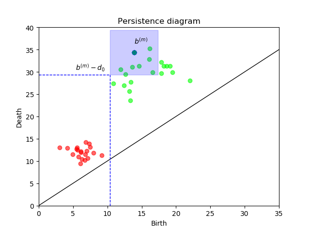
We define the function $\Theta(c):=d_{\infty}(cA,B)$. The optimal dilation $c^{*}$ is the minimizer of $\Theta(c)$ and lies in the interval $[c_{\min},c_{\max}]$. The widest interval is given by the most pessimistic scenario in terms of persistence point matching: this happens when $\mathrm{pers}(A)\ll\mathrm{pers}(B)$ and $d_{\infty}(A,B)=\mathrm{pers}(B)/2$, which means the bijective matching of points is degenerate and simply sends every point to the diagonal $\Delta$. In this case $c_{\min}=0$ and $c_{\max}=\mathrm{pers}(B)/\mathrm{pers}(A)$. We can derive a sharper bound as follows.

Let $b^{(m)}\in\chi(B)$ be the point with the longest (finite) death time. Then $b^{(m)}$ has two properties:

1. it has the largest persistence, and

2. it has the largest $y$-coordinate.

The first property (i) implies that while we are scaling $A$, we need to find a nontrivial matching point in $A$ in order to decrease the standard bottleneck distance. Thus there is at least one point lying in the box centered at $b^{(m)}$ with radius $d_{0}$. The second property (ii) guarantees we can move $A$ as far as the maximal death value in order to derive a sharper bound.

Theorem 19.

Let $b^{(m)}\in\chi(B)$ be the point with largest $y$-coordinate. If $\displaystyle c\leq\frac{b_{y}^{(m)}-d_{0}}{\mathrm{bd}(A)}$, then $\Theta(c)\geq d_{0}$. Furthermore, if $\displaystyle c\leq\min\bigg\{\frac{b_{y}^{(m)}+b_{x}^{(m)}}{2\mathrm{bd}(A)},\frac{\mathrm{pers}(B)}{\mathrm{pers}(A)}\bigg\}$, then $\displaystyle\Theta(c)=\frac{\mathrm{pers}(B)}{2}$.

Proof.

The property of largest persistence of $b^{(m)}$ implies that no point in $cA$ resides in the box around $b^{(m)}$ with radius $d_{0}$. In particular, for any point $a=(a_{x},a_{y})\in A$, note that $a_{x}\leq a_{y}\leq\mathrm{bd}(A)$ and

$$\|ca-b^{(m)}\|_{\infty}=\max\{|ca_{x}-b^{(m)}_{x}|,\,|ca_{y}-b^{(m)}_{y}|\}\geq b^{(m)}_{y}-ca_{y}>b^{(m)}_{y}-\frac{a_{y}}{\mathrm{bd}(A)}(b^{(m)}_{y}-d_{0})\geq d_{0}.$$

For any bijection $\gamma:B\to cA$, we have $\|b^{(m)}-\gamma(b^{(m)})\|_{\infty}\geq d_{0}$ so $\Theta(c)\geq d_{0}$.

Similarly, if $\displaystyle c<\frac{b_{y}^{(m)}+b_{x}^{(m)}}{2\mathrm{bd}(A)}$, for any point $a=(a_{x},a_{y})\in A$,

$$\|ca-b^{(m)}\|_{\infty}=\max\{|ca_{x}-b^{(m)}_{x}|,\,|ca_{y}-b^{(m)}_{y}|\}\geq b^{(m)}_{y}-ca_{y}>b^{(m)}_{y}-\frac{a_{y}}{2\mathrm{bd}(A)}(b^{(m)}_{y}+b^{(m)}_{x})\geq\frac{\mathrm{pers}(B)}{2}.$$

Thus for any bijection $\gamma:B\to A$, we have $\displaystyle\|b^{(m)}-\gamma(b^{(m)})\|_{\infty}\geq\frac{\mathrm{pers}(B)}{2}.$ However, the degenerate bijection sending every point to the diagonal gives $\displaystyle d_{\infty}(cA,B)\leq\max\bigg\{\frac{\mathrm{pers}(cA)}{2},\,\frac{\mathrm{pers}(B)}{2}\bigg\}\leq\frac{\mathrm{pers}(B)}{2}$. Thus, we have $\displaystyle\Theta(c)=\frac{\mathrm{pers}(B)}{2}$. ∎

This result allows us to update the lower bound of the search interval to $c_{\min}=\displaystyle\max\bigg\{\frac{b^{(m)}_{y}-d_{0}}{\mathrm{bd}(A)},\,\frac{\mathrm{pers}(B)-2d_{0}}{\mathrm{pers}(A)}\bigg\}$.

Symmetrically, by switching the roles of $A$ and $B$, we may update the upper bound of the search interval.

Theorem 20.

Let $a^{(m)}\in{\mathrm{char}}(A)$ be the point with largest $y$-coordinate. If $\displaystyle c\geq\frac{\mathrm{bd}(B)+d_{0}}{a^{(m)}_{y}}$, then $\Theta(c)\geq d_{0}$. Further, if $\displaystyle c\geq\max\bigg\{\frac{2\mathrm{bd}(B)}{a^{(m)}_{x}+a^{(m)}_{y}},\,\frac{\mathrm{pers}(B)}{\mathrm{pers}(A)}\bigg\}$, then $\displaystyle\Theta(c)=c\cdot\frac{\mathrm{pers}(A)}{2}$.

Proof.

The property of largest persistence of $b^{(m)}$ implies that no point in $B$ resides in the box around $ca^{(m)}$ with radius $d_{0}$. The calculation proceeds as above in the proof of Theorem 19. With regard to the second property of $b^{(m)}$ having the largest $y$-coordinate, if $\displaystyle c\geq\frac{2\mathrm{bd}(B)}{a^{(m)}_{x}+a^{(m)}_{y}}$, then for any point $b=(b_{x},b_{y})\in B$,

$$\|ca^{(m)}-b\|_{\infty}=\max\{|ca_{x}^{(m)}-b_{x}|,\,|ca_{y}^{(m)}-b_{y}|\} \geq ca^{(m)}_{y}-b_{y}$$

$$>c\bigg(\frac{a^{(m)}_{x}+a^{(m)}_{y}}{2}+\frac{a^{(m)}_{y}-a^{(m)}_{x}}{2}\bigg)-\mathrm{bd}(B)$$

$$\geq c\frac{\mathrm{pers}(A)}{2}=\frac{\mathrm{pers}(cA)}{2},$$

thus $\displaystyle d_{\infty}(cA,B)\geq\frac{\mathrm{pers}(cA)}{2}$. The degenerate bijection matching every persistence point to the diagonal gives $\displaystyle d_{\infty}(cA,B)\leq\max\bigg\{\frac{\mathrm{pers}(cA)}{2},\frac{\mathrm{pers}(B)}{2}\bigg\}\leq\frac{\mathrm{pers}(cA)}{2}$. Therefore, $\Theta$ is a linear function with slope $\displaystyle\frac{\mathrm{pers}(A)}{2}$. ∎

The upper bound of the search interval can now be updated to $\displaystyle c_{\max}=\min\bigg\{\frac{\mathrm{bd}(B)+d_{0}}{a^{(m)}_{y}},\,\frac{\mathrm{pers}(B)+2d_{0}}{\mathrm{pers}(A)}\bigg\}$.

As a consequence of Theorems 19 and 20, we obtain the following characterization for the function $\Theta$, which is independent of the data.

Proposition 21.

Set $\displaystyle c_{B}=\min\bigg\{\frac{b_{y}^{(m)}+b_{x}^{(m)}}{2\mathrm{bd}(A)},\,\frac{\mathrm{pers}(B)}{\mathrm{pers}(A)}\bigg\}$ and $\displaystyle c_{A}=\max\bigg\{\frac{2\mathrm{bd}(B)}{a^{(m)}_{x}+a^{(m)}_{y}},\,\frac{\mathrm{pers}(B)}{\mathrm{pers}(A)}\bigg\}$. Then

$$\Theta(c)=\begin{cases}\text{ is constant at }\frac{\mathrm{pers}(B)}{2}&\text{ for }0\leq c\leq c_{B};\\ \text{ attains the minimum }\overline{d_{D}}(A,B)&\text{ for }c_{B}\leq c<c_{A};\\ \text{ is linear with }c\cdot\frac{\mathrm{pers}(A)}{2}&\text{ for }c_{A}\leq c.\end{cases}$$

This behavior is consistent with our findings in applications to real data as we will see in Section 4.

3.2 Computing Dilation-Invariant Bottleneck Distances

Using the same framework as for the dilation-invariant bottleneck dissimilarity previously, we can similarly derive a direct search algorithm for the computation of dilation-invariant bottleneck distance $D_{S}$ as follows: following Theorems 19 and 20, for any two persistence diagrams $A$ and $B$, set

$$s_{B} ={\rm log}(b^{(m)}_{y})-{\rm log}(\mathrm{bd}(A))-d_{\infty}({\rm log}(A),{\rm log}(B))$$

$$s_{A} ={\rm log}(\mathrm{bd}(B))-{\rm log}(a^{(m)}_{y})+d_{\infty}({\rm log}(A),{\rm log}(B))$$

and search for the optimal shift $s^{*}$ in the interval $[s_{B},s_{A}]$.

An alternative approach to computing the dilation-invariant bottleneck distance is to adopt the kinetic data structure approach proposed by Sheehy et al. (2018) to compute the shift-invariant bottleneck distance. This method iteratively updates the matching value until the event queue is empty. When the loop ends, it attains the minimum which is exactly $D_{S}$. The algorithm runs in $O(n^{3.5})$ time where $n$ is the number of points in the persistence diagrams.

We remark here that our proposed direct search algorithm runs in $O(Nn^{1.5}{\rm log}n)$ time, which is a significant improvement over the kinetic data structure approach to compute the shift-invariant bottleneck distance. On the other hand, the optimal value that we obtain is approximate, as opposed to being exact.

3.2.1 Performance Comparison

We compared both algorithms on simulated persistence diagrams; results are displayed in Table 1. Note that in general, persistence diagrams contain points with 0 birth time which will cause an error of a $-\infty$ value when taking logs; we bypassed this difficulty by adding a small constant to all persistence intervals (in this test, the constant we used was $10^{-10}$). This correction may be used for a general implementation of our method to compute dilation-invariant bottleneck distances. For the direct search algorithm, we fixed the number of partitions to be 100 in each test and used the inline function bottleneck-distance in GUDHI. The time comparison experiments were run on a PC with Intel(R) Core(TM) i7-6500U CPU @ 2.50GHz and 4 GB RAM; runtimes are given in wall-time seconds.

Table 1: Comparison of the Direct Search (DS) Algorithm and the Kinetic Data Structure (KDS) Algorithm

Number of Points	Original Distance	KDS Distance	DS Distance	KDS Runtime	DS Runtime
32	8.9164	6.9489	7.0635	1.8105	0.1874
64	7.4414	6.9190	6.9572	17.0090	0.3280
128	0.5545	0.5407	0.5407	146.1578	0.6547
256	1.6291	1.3621	1.3800	767.4551	1.4373
512	2.3304	1.9330	1.9459	12658.2584	3.3468
1785	6.3851	3.1925	3.2511	614825.1576	51.1568

An immediate observation is the vastly reduced runtime of our proposed direct search algorithm over the kinetic data structure-based algorithm, particularly when the number of persistence points in the diagrams increases. An additional observation is that our direct search algorithm tends to estimate conservatively and systematically return a distance that is larger than that returned by the kinetic data structure approach, which is known to give the exact value. The difference margins between the two distances also tends to decrease as the number of persistence points in the diagrams increases. Overall, we find that our direct search approach finds accurate results that are consistent with the exact values far more efficiently; when exact values are not required, the accuracy versus efficiency trade-off is beneficial.

We plotted the differences in the logs of the runtime and the number of persistence points to evaluate the time complexity of the two algorithms in practice, shown in Figure 4. The slope of each straight line gives the order of the computational complexity for each algorithm. We see that in our set of experiments, the empirical complexity is actually lower than, but still close to, the theoretical complexity bounds.

Figure 4: Plot of ${\rm log}({\rm time})-{\rm log}(\#{\rm points})$ for both search algorithms based on simulated persistence diagrams. The slopes match the theoretical orders of complexity.

Software and Data Availability

Software to compute the dilation-invariant bottleneck dissimilarity and to reproduce all results in this paper are available at https://github.com/antheamonod/Dilation_invariant_bottleneck.

4 Application to Data and Results

We present two applications to data: one is an exploratory analysis, where we evaluate our approach on two datasets that have a known hierarchical and network structure; the other is an example of inference where we perform topology-based information retrieval based on the dilation-invariant bottleneck distance.

4.1 Exploratory Analysis: Database Representation for Information Retrieval

We apply persistent homology to study the database structures in their manifold-embedded representations rather than on the graphs themselves. Although persistent homology has been computed directly on graphs and networks (for instance, in applications in neuroscience (Patania et al., 2019, e.g.,)), manifolds may be equipped with a larger variety of metrics than graphs; moreover, on a manifold, distances may be defined between arbitration points along any path, while on a graph, we are constrained to traveling only along the graph edges. Since the metric is a fundamental component in computing persistent homology, it is desirable to work in a setting where we may study a variety of metrics in a computationally efficient manner to obtain a better understanding of the persistence structure of the databases.

In IR, a dataset $Ds:=\{d_{1},...,d_{N}\}$ consisting of $N$ data points is embedded in a latent manifold $M$ via a model $f$. A query $q$ is then embedded in the same space and compared against all or a subset of the elements of $Ds$ via a distance metric $d$. The $m$ closest matches are then returned. Formally, the returned set $Rs$ is defined as $Rs=\min_{m}\{d(f(Ds),f(q))\}$. The local structure of the space as well as the global connectivity of the dataset $Ds$ is of paramount importance in IR. Persistent homology is able to characterize both the global and local structure of the embedding space.

Following Nickel and Kiela (2017), we embed the hierarchical graph structure of our datasets onto a Euclidean manifold and a Poincaré ball by minimizing the loss function

$$\mathcal{L}=\sum_{(u,v)\in\mathcal{H}}{\rm log}\frac{e^{-d(u,v)}}{\sum_{v^{\prime}\in\mathcal{N}(u)}e^{-d(u,v^{\prime})}},$$ (17)

where $d$ is the distance of the manifold $M$, $\mathcal{H}$ is the set of hypernymity relations, and $\mathcal{N}=\{v^{\prime}\mid(u,v^{\prime})\notin D\}\cup\{v\}$, thus the set of negative examples of $u$ including $v$.

In the case of the Euclidean manifold, we use two metrics: the standard $L_{2}$ distance and the cosine similarity,

$$sim(x,y)=\frac{xy}{\|x\|\|y\|},$$

which has been used in inference in IR Scarlini et al. (2020); Yap et al. (2020). On the Poincaré ball, the distance is given by

$$d_{P}(x,y)=\cosh^{-1}\left(1+\frac{2\|x-y\|^{2}}{(1-\|x\|^{2})(1-\|y\|^{2})}\right),$$ (18)

where $\|\cdot\|$ is the standard Euclidean norm. We optimize our model (17) directly on each of the manifolds with respect to these three metrics.

For the Poincaré ball, in addition to studying the direct optimization, we also study the representation of the Euclidean embedding on the Poincaré ball. The Euclidean embedding is mapped to the Poincaré ball using the exponential map (Mathieu et al., 2019):

$$\exp_{x}^{c}(z)=x\oplus_{c}\left[\tanh\left(\frac{\sqrt{c}\,\lambda_{x}^{c}\|z\|}{2}\right)\frac{\hat{z}}{\sqrt{c}}\right],$$

where $\hat{z}:=z/||z||$, $\lambda_{x}^{c}:=2/(1-c\|x\|^{2})$, and $\oplus_{c}$ denotes Möbius addition under the curvature $c$ of the manifold (Ganea et al., 2018). Here, we take $c=-1$.

We calculate the VR persistent homology of the four embeddings to evaluate the current IR inference approaches from a topological perspective. Since we work with real-valued data, the maximum dimension for homology was set to 3. All persistent homology computations in this work were implemented using giotto-tda (Tauzin et al., 2020). We note here that since VR persistent homology is computed, Ripser is available for very large datasets (Bauer, 2021). Ripser is currently the best-performing software for VR persistent homology computation both in terms of memory usage and wall-time seconds (3 wall-time seconds and 2 CPU seconds to compute persistent homology up to 2 dimensions of simplicial complexes of the order of $4.5\times 10^{8}$ run on a cluster, 3 wall-time seconds for the same dataset run on a shared memory system) (Otter et al., 2017).

ActivityNet.

ActivityNet is an extensive labeled video dataset of 272 human actions that are accompanied by a hierarchical structure, visualized in Figure 5 (Heilbron et al., 2015). This dataset has been previously used in IR (Long et al., 2020).

Figure 5: Visualization of ActivityNet Dataset. Note that hierarchical structure of the dataset naturally exhibits interesting topological properties such as cycles, clusters, and a tree-like structure.

Mammals of WordNet.

WordNet is a lexical database that represents the hierarchy of the English language in a tree-like form, which has been extensively used in NLP (Miller, 1995). In our application, we focus on the subportion of WordNet relating to mammals. We pre-process this dataset by performing a transitive closure (Nickel and Kiela, 2017).

Embedding the Data. Both datasets were embedded in a 5-dimensional space, following Nickel and Kiela (2017). For both datasets, we trained the models for 1200 epochs with the default hyperparameters. For ActivityNet, we were able to achieve hypernimity mAP of $94.3\%$ and $97.2\%$ for the Euclidean manifold and Poincaré ball, respectively; while for the Mammals data, we achieved $45\%$ and $82.3\%$, respectively. These results are consistent with Nickel and Kiela (2017).

4.1.1 Topology of the Euclidean Embeddings

The persistence diagrams of the Euclidean embeddings under both metrics and for both datasets are given in Figure 6. We see that up to scaling, the persistence diagrams for both embeddings into Euclidean space with respect to the $L_{2}$ metric and cosine similarity are similar in terms of location and distribution of $H_{0}$, $H_{1}$, and $H_{2}$ points on the persistence diagrams. We quantify this similarity by computing dilation-invariant bottleneck dissimilarities. The graphs of the search procedure for each dataset are given in Figure 8. We first note that the standard bottleneck distances between the $L_{2}$ and cosine similarity persistence diagrams are $1.642$ for the ActivityNet dataset, and $0.6625$ for the Mammals dataset. The dilation-invariant bottleneck dissimilarities are achieved at the minimum value of the bottleneck distance in our parameter search region. The dilation-invariant bottleneck dissimilarities from cosine similarity to $L_{2}$ are $1.311$ for the ActivityNet dataset and $0.3799$ for the Mammals dataset.

The dilation parameter for Euclidean embeddings can be alternatively searched according to the scale of $L_{2}$ embedded points as follows. Since mutual distances under the cosine embedding are always bounded by 1, we can regard the induced finite metric space as a baseline. For the $L_{2}$ embedding, mutual dissimilarities are affected by the scale of the embedded point cloud, i.e., if we multiply the points by a factor $R$, the induced metric will also dilate by a factor $R$. In experiments, the scale is $18.13$ for the $L_{2}$ embedding of ActivityNet and $3.188$ for Mammals, which are consistent with dilation parameters we found.

The visual compatibility of the persistence diagrams together with the small dilation-invariant bottleneck distances indicate that the topology of the database is preserved in the Euclidean embedding, irrespective of the metric.

Figure 6: Persistence Diagrams of Euclidean Embeddings. AN: ActivityNet, M: Mammals.

4.1.2 Topology of the Poincaré Ball Embeddings

The persistence diagrams for the Poincaré ball embeddings for both datasets are given in Figure 7. For the ActivityNet dataset, we see that both embeddings fail to identify the $H_{1}$ and $H_{2}$ homology inherent in the dataset (see Figure 5), which, by contrast, the Euclidean embeddings successfully capture. For the Mammals dataset, only the exponential map embedding into the Poincaré ball is able to identify $H_{1}$ and $H_{2}$ homology, but note that these are all points close to the diagonal. Their position on the diagonal indicates that the persistence of their corresponding topological features is not significant: these features are born and die almost immediately, are therefore likely to be topological noise. We now investigate this phenomenon further.

Figure 7: Persistence Diagrams of Poincaré Embeddings. AN: ActivityNet, M: Mammals, expmap signifies Euclidean optimization followed by an exponential map embedding into the Poincaré ball, while Poincaré signifies direct optimization on the Poincaré ball.

From (18), we note that an alternative representation for the distance function maybe obtained as follows. Set

$$A(x,y):=1+\frac{2\|x-y\|^{2}}{(1-\|x\|^{2})(1-\|y\|^{2})},$$ (19)

then (18) may be rewritten as

$$d_{P}(x,y)={\rm log}(A(x,y)+\sqrt{A(x,y)^{2}-1}).$$ (20)

((a)) AN Poincaré

((b)) M Poincaré

((c)) AN Euclidean

((d)) M Euclidean

Figure 8: Dilation-Invariant Bottleneck Distances Between Embeddings. AN: ActivityNet, M: Mammals

We assume that $\|x-y\|$ has a strictly positive lower bound and study the case when both points $x,y$ lie near the boundary, i.e., both $\|x\|\approx 1$ and $\|y\|\approx 1$. Notice, then, that (19) and (20) are approximated by

$$A(x,y) \approx\frac{1}{2}\frac{\|x-y\|^{2}}{(1-\|x\|)(1-\|y\|)},$$

$$d_{P}(x,y) \approx{\rm log}(2A(x,y))$$

$$\approx 2{\rm log}(\|x-y\|)-{\rm log}(1-\|x\|)-{\rm log}(1-\|y\|).$$ (21)

Notice also that

$$d_{P}(x,0)\approx{\rm log}2-{\rm log}(1-\|x\|).$$ (22)

Combining (21) and (22) yields the following approximation for the Poincaré distance:

$$d_{P}(x,y)\approx d_{P}(x,0)+d_{P}(y,0)+2{\rm log}(\|x-y\|/2).$$ (23)

For points near the boundary, i.e., $d_{P}(x,0)=R\gg 1$, (23) gives a mutual distance of approximately $2R$ between any given pair of points.

Recall from Definition 2 that a $k$-simplex is spanned if and only if the mutual distances between $k+1$ points are less than a given threshold $r$. The implication for discrete points near the boundary of the Poincaré ball is that either the threshold is less than $2R$, and then the VR complex is a set of 0-simplices; or the threshold is greater than $2R$, and then the VR complex is homeomorphic to a simplex in higher dimensions. That is, the VR filtration jumps from discrete points to a highly connected complex; this behavior is illustrated in Figure 9.

Figure 9: Illustration of connectivity behavior in a VR complex on the Poincaré ball equipped with the Poincaré distance. For points sampled near the boundary, the connectivity of the VR complex grows slowly at low threshold values (small radii) and quickly becomes highly connected as the threshold grows and we approach the approximation (23) for distances between points.

((a)) Empirical CDF

((b)) Population CDF

Figure 10: Cumulative distribution functions (cdf) of edges in a VR complex with respect to Poincaré and Euclidean distances. (a) Proportion of edges in a VR filtration with respect to the Poincaré distance on the Poincaré ball (blue lines) and the Euclidean distance on Euclidean space (red lines), computed (24), against scaled VR threshold values Definition 2. (b) Population cdf as derived in Theorems 23 and 24.

This phenomenon of sharp phase transition is observable in our applications, which we further explore through numerical experiments and display in Figure 10. Here, each curve corresponds to a numerical experiment. We also plot the corresponding connectivity of VR complexes with respect to the Euclidean distance for comparison. For a given experiment, we draw the distance cumulative distribution function as follows: first, we normalize distances and sort them in ascending order; next, for the $k$th element $R_{k}$, we compute the proportion of connected pairs as

$$\frac{\#\{(x_{i},x_{j})\mid d_{P}(x_{i},x_{j})\leq R_{k}\}}{\#\{(x_{i},x_{j})\}}.$$ (24)

From the cumulative distribution plot in Figure 10, we see this rapidly increasing connectivity behavior at higher threshold values in repeated numerical experiments. In each experiment, points are sampled closer and closer to the boundary of the ball, and we see a progressively sharper jump in connectivity of the VR complex the closer to the boundary the points lie for the Poincaré distance. For the extreme case with points sampled closest to the boundary of the ball, when the VR threshold value is at $90\%$ of the maximum distance, there are less than $10\%$ pairs of points that are connected. This percentage sharply and dramatically increases at thresholds from 90% to the maximum distance, from $10\%$ to $100\%$ of pairs of points being connected. The phase change explains why we cannot see long persistence (in terms of points appearing far away from the diagonal) in dimension 1 or 2 in Figure 7. The connectivity of the VR complex under the Euclidean distance, in contrast, grows linearly with the threshold. Moreover, we see that the connectivity is stable and robust to the sampling location of the points since there is very little variability in the curves; the linear growth in connectivity is unaffected by the location of the sampled points. We now formalize these observations.

Statistical Properties of VR Edges on the Poincaré Ball.

Since edges in a VR complex are determined by distances between vertices, we are interested in studying the distributions of the distances measured by the Euclidean (standard $L_{2}$ distance) $d_{E}$ and Poincaré $d_{P}$ metrics on the ball. Let $\mathbb{S}^{1}(r)$ be a circle of radius $r$ (measured in Euclidean distance); then any point on $\mathbb{S}^{1}(r)$ takes the form of $re^{i2\pi\theta}$. Let $\theta_{X}$ and $\theta_{Y}$ be two independent random variables uniformly distributed on $\mathbb{R}/\mathbb{Z}=[0,1)$; and set $X:=re^{i2\pi\vartheta_{X}}$ and $Y:=re^{i2\pi\theta_{Y}}$ so that $X$ and $Y$ are $\mathbb{S}^{1}(r)$-valued random variables. We now characterize the distributions of $d_{E}(X,Y)$ and $d_{P}(X,Y)$.

Lemma 22.

Let $\theta_{X},\theta_{Y}\sim\mathrm{Unif}(\mathbb{R}/\mathbb{Z})$. Then $Z:=\theta_{Y}-\theta_{X}\sim\mathrm{Unif}(\mathbb{R}/\mathbb{Z})$.

Proof.

For any $a\in[0,1]$, observe that

$$\mathbb{P}(Z\leq a) =\sum_{n\in\mathbb{Z}}\mathbb{P}(n\leq\theta_{Y}-\theta_{X}\leq a+n)$$

$$=\mathbb{P}(0\leq\theta_{Y}-\theta_{Z}\leq a)+\mathbb{P}(-1\leq\theta_{Y}-\theta_{X}\leq a-1)$$

$$=\frac{1}{2}-\frac{1}{2}(1-a)^{2}+\frac{1}{2}a^{2}=a,$$

as desired. ∎

The cumulative distribution function (cdf) of the Euclidean distance between $X$ and $Y$ can be explicitly derived as follows.

Theorem 23.

Let $F_{E}:[0,1]\rightarrow[0,1]$ denote the cdf of the normalized Euclidean distance $\frac{1}{2r}d_{e}(X,Y)$ between $X$ and $Y$. Then for all $t\in[0,1]$,

$$F_{e}(t)=\frac{2}{\pi}\sin^{-1}(t).$$

Proof.

First notice that

$$d_{E}(X,Y) =r\sqrt{(\cos(2\pi\theta_{X})-\cos(2\pi\theta_{Y}))^{2}+(\sin(2\pi\theta_{X})-\sin(2\pi\theta_{Y}))^{2}}$$

$$=r\sqrt{2-2\cos(2\pi(\theta_{Y}-\theta_{Z}))}$$

$$=2r\sin(\pi Z).$$ (25)

Then we have

$$F_{e}(t)=\mathbb{P}\bigg(\frac{1}{2r}d_{E}\leq t\bigg)=\mathbb{P}(\sin(\pi Z)\leq t)=\frac{2}{\pi}\sin^{-1}(t).$$ (26)

∎

Notice that the cdf does not depend on $r$, which is consistent with what we observe in numerical experiments given in Figure 10. We now derive the cdf for Poincaré distance $d_{P}$ between $X$ and $Y$.

Theorem 24.

Let $M:=\max\{d_{P}(X,Y)\}$ and let $F_{P}:[0,1]\rightarrow[0,1]$ be the cdf of the normalized Poincaré distance $\frac{1}{M}d_{P}(X,Y)$. Then for all $t\in[0,1]$,

$$F_{P}(t)=\frac{2}{\pi}\sin^{-1}\bigg(\frac{1}{2}\sinh\bigg(\frac{tM}{2}\bigg)\bigg(\frac{1}{r}-r\bigg)\bigg).$$

Proof.

We have

$$d_{P}(X,Y)=\cosh^{-1}\bigg(1+\frac{2d_{E}(X,Y)^{2}}{(1-r^{2})^{2}}\bigg)=\cosh^{-1}\bigg(1+\frac{8r^{2}\sin^{2}(\pi Z)}{(1-r^{2})^{2}}\bigg)=2\sinh^{-1}\bigg(\frac{2\sin(\pi Z)}{\frac{1}{r}-r}\bigg),$$

by substituting (25) above. We then have that $\displaystyle M=2\sinh^{-1}\bigg(\frac{2}{\frac{1}{r}-r}\bigg)$ and compute, using (26):

$$F_{P}(t) =\mathbb{P}(d_{P}(X,Y)\leq tM)$$

$$=\mathbb{P}\bigg(d_{E}(X,Y)^{2}\leq\frac{(1-r^{2})^{2}(\cosh(tM)-1)}{2}\bigg)$$

$$=\mathbb{P}\bigg(\sin(\pi Z)\leq\frac{1}{2}\sinh\bigg(\frac{tM}{2}\bigg)\bigg(\frac{1}{r}-r\bigg)\bigg)$$

$$=\frac{2}{\pi}\sin^{-1}\bigg(\frac{1}{2}\sinh\bigg(\frac{tM}{2}\bigg)\bigg(\frac{1}{r}-r\bigg)\bigg).$$

∎

Notice that contrary to the Euclidean case given by Theorem 23 above, here, the cdf depends on the radius $r$. More precisely, let $r_{n}$ be a sequence of radius values converging to 1 and here, let $R_{n}:=\frac{1}{M_{n}}d_{P}(X_{n},Y_{n})$, where $M_{n},X_{n},Y_{n}$ are the corresponding $M,X,Y$ values associated with the radius $r_{n}$; let $F_{P}^{(n)}$ be the cdf of each $R_{n}$. Then

$$F_{P}^{(n)}(t)\rightarrow F^{\infty}(t)=\begin{cases}1,&t=1;\\ 0,&0\leq t<1.\end{cases}$$

In other words, we have that $R_{n}$ converges in distribution to the Dirac delta $\delta_{1}$.

Note that although the topology of the databases is not captured in the Poincaré ball embeddings, the dilation-invariant bottleneck dissimilarity for the ActivityNet embedding is nevertheless small, with a value of $0.5481$ and corresponding dilation parameter value of $3.986$. We do not see this coincidence for the Mammals dataset, however: the dilation-invariant bottleneck dissimilarities between the persistence diagram arising from the exponential map embedding and the direct Poincaré embedding remains large at $5.808$ with a corresponding dilation parameter value of $3.182$. This large dilation-invariant bottleneck dissimilarity is likely due to the difference in occurrences of homology between the two diagrams: the exponential map embedding picks up on spurious $H_{1}$ and $H_{2}$ homology, while the direct Poincaré embedding does not. There is no immediate interpretation for the dilation parameter value and its effect on the dilation-invariant bottleneck dissimilarities, due to the nonlinear and asymmetric behavior of the comparison measure and derived approximations (see Figure 9).

Overall, we find that the higher-order connectivity and hierarchy of the databases was preserved in the Euclidean embeddings, but not in the Poincaré ball embeddings: $H_{1}$ and $H_{2}$ homology corresponding to cycles and voids appear in the persistence diagrams of the Euclidean embeddings, and do not in the Poincaré ball embeddings.

4.2 Symmetry versus Asymmetry in Practice

Here, we give a demonstration with real data on the difference between assuming a symmetric versus asymmetric dilation-invariant bottleneck dissimilarity as discussed previously in Section 2.4. We compute both the asymmetric (5) and symmetric (14) dilation-invariant bottleneck dissimilarities for the persistence diagrams of the ActivityNet and Mammals datasets to the Euclidean embedding with $L_{2}$ metric of the Mammals dataset (which we denote as M $L_{2}$); the results are given in Table 2.

	AN Cosine	AN $L_{2}$	AN+expmap	AN Poincaré	M Cosine	M+expmap	M Poincaré
$\overline{d_{D}}$	0.38	0.45	0.57	0.49	0.39	0.21	0.44
$\overline{d_{\mathrm{sym}}}$	0.23	0.93	3.02	1.24	0.23	0.61	3.27

Table 2: Symmetric and asymmetric dilation-invariant bottleneck dissimilarities between persistence diagrams of all embeddings to the persistence diagram of the Euclidean with $L_{2}$ distance embedding of the Mammals dataset.

Using the asymmetric dilation-invariant bottleneck dissimilarity, the most similar persistence diagram to that of the M $L_{2}$ embedding is the persistence diagram of the M+expmap embedding with a value of 0.21. It also finds that persistence diagrams of other embeddings of the Mammals dataset are close as well (0.39 and 0.44).

Using the symmetric dilation-invariant bottleneck dissimilarity, the most similar persistence diagrams to that of the M $L_{2}$ embedding are the persistence diagrams of the AN Cosine and M Cosine embedding (0.23). However, the persistence diagram of the M Poincaré dataset has a comparatively large dissimilarity (3.27). This is because $\overline{d_{D}}(A,B)$ depends on the scale of the second variable (persistence diagram) $B$. When comparing dissimilarities, it only makes sense if everything is compared under the same scale (i.e., fix $B$). If we symmetrize, the scales of $A$ and $B$ mix up and the result becomes uninterpretable. In the above example, the persistence diagram of the M Poincaré embedding has much larger scale than the persistence diagram of the M $L_{2}$ embedding. Though these two datasets have similar topology as shown using the asymmetric dilation-invariant bottleneck dissimilarity, the symmetric version is not able to identify this resemblance.

4.3 Topological Information Retrieval: A Classification Problem

We now turn to a problem of inference: specifically, we perform an IR task at the database level taking into account the inherent topology of the database. For this task, we use seven medical imaging databases from MedMNIST (Yang et al., 2021); summaries of these datasets are given in Table 3. The task is the following: Given a set of points $N$, we seek the closest set of points $M$ where $N\ll M$ such that the two sets comprise representatives from the same category. Essentially, this problem may be approached as a problem of topological classification. Persistent homology has been successfully used in various classification problems and settings, including trajectory classification in robotics (Pokorny et al., 2014), determination of parameters of dynamical systems (Adams et al., 2017), and sleep-wake classification in physiology (Chung et al., 2021). In particular, it has been used in medical imaging classification for endoscopy images (Dunaeva et al., 2016), prostate cancer histopathology images (Lawson et al., 2019), and liver biopsy tissue images (Teramoto et al., 2020).

Dataset	Derma	Pneumonia	Retina	Breast	Organ_Axial	Organ_Coronal	Organ_Sagittal
Classes	7	2	5	2	11	11	11
Samples	10,015	5,856	1600	780	58,850	23,660	25,221

Table 3: Characteristics of MedMNIST datasets

Using an autoencoder based upon Hou (2019), we embedded each dataset separately in Euclidean space. We note in particular that the networks do not provide explicit information regarding the class of each input image. Since the number of embedding points exceeded the reasonable computational time frame threshold for VR persistent homology (see Table 3), we obtained persistence diagram representatives of embeddings of each class as follows: we split the embeddings on non-overlapping sets of $N=\{500,600\}$ and computed the class-specific persistence diagram by the multiple subsampling scheme described by Chazal et al. (2015). Specifically, for a large dataset $X$ with $M$ points, we sample $m\ll M$ points randomly $B$-many times. The procedure yields $B$ point sets, $X_{1},\cdots,X_{B}$, which then give the persistence diagrams $\mathrm{Dgm}(X_{1}),\cdots,\mathrm{Dgm}(X_{B})$. The Fréchet mean (also referred to as the Lagrangian barycenter (Lacombe et al., 2018)) is given by

$$\overline{\mathrm{Dgm}}=\mathop{\arg\min}_{Z\in\mathcal{D}}\frac{1}{B}\sum_{i=1}^{B}d_{2}(Z,\,\mathrm{Dgm}(X_{i}))^{2}$$

where $d_{2}$ is the 2-Wasserstein distance between persistence diagrams, which we compute following Turner et al. (2014). In similar spirit to Chazal et al. (2015), we take the Fréchet mean $\overline{\mathrm{Dgm}}$ to approximate $\mathrm{Dgm}(X)$.

During inference, we randomly sample a subset of proportion $\{0.2,0.4,0.6,0.8\}$ of the class, compute VR persistence, and compare to the class-specific persistence diagrams using our dilation-invariant bottleneck dissimilarity. The class of the most similar persistence diagram (i.e., the one with the smallest dilation-invariant bottleneck dissimilarity) is assigned to the query subset.

In Table 4, we show the classification results where we quote the Top 1st and Top 2nd accuracy of our predictions, i.e., whether or not the correct class is in the 1st or 2nd predicted position based on the ordered similarity. We note that with our the dilation-invariant bottleneck dissimilarity, we are able to predict the correct class with an accuracy of up to $87\%$. As expected, the more points we have in our query, the better the accuracy since the query persistence diagram is then a better representative of the true persistence diagram. We further notice a slight drop in performance in some datasets for the $60\%$ proportion, which we hypothesize is due to suboptimal sampling from the embeddings. Notice here that since we are querying by persistence diagrams, we are effectively querying by sets, so there is no appropriate comparative measure in terms of other methods; the most appropriate comparison for our performance is the same IR task but using the standard bottleneck distance. We find that our method matches or outperforms the standard bottleneck distance in the same IR task, especially in datasets with more classes when using less data to compute the persistence diagram.

5 Discussion

In this work, we used persistent homology to quantify and study the topological structure of databases corresponding to their hierarchy and connectivity as an exploratory analysis. We found that the Euclidean embeddings preserve the topology of the databases with respect to both the $L_{2}$ and cosine similarity metrics, while the Poincaré ball embeddings did not. Moreover, we found that among topology-preserving embeddings, the topological structure captured by the persistence diagrams was consistent. To quantify this effect, we introduced the dilation-invariant bottleneck dissimilarity and distance, which retains the resemblance between persistence diagrams and erases the distortion effect of the different metrics over the embeddings. We found that dilation-invariant bottleneck distances between topology-preserving database representations are small in our exploratory analysis. We further performed an IR task of classification using the dilation-invariant bottleneck distance and found a high level of accuracy of classification. Our work is, to the best of our knowledge, the first application of TDA in IR.

Note that in our exploratory analysis and in studying the topology of the database representations, the goal of our work was to evaluate how different metric spaces maintain the topology of databases without any prior incentive to do so. This is in contrast to previous work where TDA has been applied to hierarchical database representations and compactifications, such as work by Aloni et al. (2021) who impose geometric and topological structures and work by Moor et al. (2020) who explicitly enforce a topological constraint. Our motivation for not imposing any topological structure is with task of IR in mind: while “bad” databases may need their topology to be enforced, for “good” databases, this is not necessary. In this work, we do not seek to improve the topological quality of the database representations. Our results presented here are a first step in assessing the utility of TDA as a viable tool in IR, which was indeed demonstrated in Section 4.3. Our findings show that without enforcing a topological prior, the topology is not preserved between two commonly-used embeddings to a high degree, which we quantify with the dilation-invariant bottleneck distance. Where the connectivity of the database is important, i.e., when we seek to preserve cycles and higher order topology, database embeddings into the Poincaré ball are less desirable. While embeddings into the Poincaré ball indeed preserve hierarchy and are useful when the databases are known to be trees, when it is a priori unknown if there exists a higher order structure that would be important for IR, our work shows that a more conservative approach would be to use an alternative embedding.

Our findings motivate the quantification of the added information and potential of increased accuracy in IR tasks when taking into account the topology of the hierarchy. The initiation toward this direction shown by our inferential analysis where IR was performed by classification is promising. Fully harnessing the potential of TDA in IR tasks will entail the development of a new set of topological quality control and performance criteria, which will need to be interpretable in context and comparable to currently used methods. These criteria will need to be applied to both the queries submitted and the database, since queries are not always informative or well-designed, while databases may also suffer from missing or repeated entries and noise. An extensive set of experiments is required to assess all possible scenarios (i.e., for when queries are “bad,” but the database is “good,” and vice versa; and also when both the query and database are “bad.”). In future work, we aim to develop a topological criterion for preference of certain database embeddings over others, which may then be used to increase the precision of IR.

References

- Adams and Carlsson (2015) Adams, H. and G. Carlsson (2015). Evasion paths in mobile sensor networks. The International Journal of Robotics Research 34(1), 90–104.
- Adams et al. (2017) Adams, H., T. Emerson, M. Kirby, R. Neville, C. Peterson, P. Shipman, S. Chepushtanova, E. Hanson, F. Motta, and L. Ziegelmeier (2017). Persistence images: A stable vector representation of persistent homology. Journal of Machine Learning Research 18.
- Aloni et al. (2021) Aloni, L., O. Bobrowski, and R. Talmon (2021). Joint Geometric and Topological Analysis of Hierarchical Datasets. arXiv preprint arXiv:2104.01395.
- Anderson et al. (2018) Anderson, K. L., J. S. Anderson, S. Palande, and B. Wang (2018). Topological Data Analysis of Functional MRI Connectivity in Time and Space Domains. In G. Wu, I. Rekik, M. D. Schirmer, A. W. Chung, and B. Munsell (Eds.), Connectomics in NeuroImaging, Cham, pp. 67–77. Springer International Publishing.
- Aukerman et al. (2020) Aukerman, A., M. Carrière, C. Chen, K. Gardner, R. Rabadán, and R. Vanguri (2020). Persistent Homology Based Characterization of the Breast Cancer Immune Microenvironment: A Feasibility Study. In S. Cabello and D. Z. Chen (Eds.), 36th International Symposium on Computational Geometry (SoCG 2020), Volume 164 of Leibniz International Proceedings in Informatics (LIPIcs), Dagstuhl, Germany, pp. 11:1–11:20. Schloss Dagstuhl–Leibniz-Zentrum für Informatik.
- Bauer (2021) Bauer, U. (2021, February). Ripser: efficient computation of Vietoris–Rips persistence barcodes. Preprint.
- Bevilacqua and Navigli (2020) Bevilacqua, M. and R. Navigli (2020). Breaking through the 80% glass ceiling: Raising the state of the art in word sense disambiguation by incorporating knowledge graph information. In Proceedings of the 58th Annual Meeting of the Association for Computational Linguistics, Online, pp. 2854–2864. Association for Computational Linguistics.
- Bobrowski et al. (2017) Bobrowski, O., M. Kahle, and P. Skraba (2017, 08). Maximally persistent cycles in random geometric complexes. Ann. Appl. Probab. 27(4), 2032–2060.
- Boudin et al. (2020) Boudin, F., Y. Gallina, and A. Aizawa (2020, July). Keyphrase generation for scientific document retrieval. In Proceedings of the 58th Annual Meeting of the Association for Computational Linguistics, Online, pp. 1118–1126. Association for Computational Linguistics.
- Brüel-Gabrielsson et al. (2019) Brüel-Gabrielsson, R., B. J. Nelson, A. Dwaraknath, P. Skraba, L. J. Guibas, and G. Carlsson (2019). A Topology Layer for Machine Learning.
- Buchet et al. (2016) Buchet, M., F. Chazal, S. Y. Oudot, and D. R. Sheehy (2016). Efficient and robust persistent homology for measures. Computational Geometry 58, 70–96.
- Burago et al. (2001) Burago, D., I. D. Burago, Y. Burago, S. Ivanov, S. V. Ivanov, and S. A. Ivanov (2001). A course in metric geometry, Volume 33. American Mathematical Soc.
- Carlsson (2009) Carlsson, G. (2009). Topology and Data. Bulletin of the American Mathematical Society 46(2), 255–308.
- Chazal et al. (2009) Chazal, F., D. Cohen-Steiner, L. J. Guibas, F. Mémoli, and S. Y. Oudot (2009). Gromov–Hausdorff Stable Signatures for Shapes using Persistence. Computer Graphics Forum 28(5), 1393–1403.
- Chazal et al. (2015) Chazal, F., B. Fasy, F. Lecci, B. Michel, A. Rinaldo, and L. Wasserman (2015). Subsampling methods for persistent homology. In International Conference on Machine Learning, pp. 2143–2151. PMLR.
- Chazal et al. (2013) Chazal, F., L. J. Guibas, S. Y. Oudot, and P. Skraba (2013). Persistence-Based Clustering in Riemannian Manifolds. J. ACM 60(6).
- Chung et al. (2021) Chung, Y.-M., C.-S. Hu, Y.-L. Lo, and H.-T. Wu (2021). A persistent homology approach to heart rate variability analysis with an application to sleep-wake classification. Frontiers in Physiology 12, 202.
- Clementini et al. (1994) Clementini, E., J. Sharma, and M. J. Egenhofer (1994). Modelling topological spatial relations: Strategies for query processing. Computers & Graphics 18(6), 815–822.
- Cohen-Steiner et al. (2007) Cohen-Steiner, D., H. Edelsbrunner, and J. Harer (2007). Stability of persistence diagrams. Discrete & computational geometry 37(1), 103–120.
- Crawford et al. (2020) Crawford, L., A. Monod, A. X. Chen, S. Mukherjee, and R. Rabadán (2020). Predicting Clinical Outcomes in Glioblastoma: An Application of Topological and Functional Data Analysis. Journal of the American Statistical Association 115(531), 1139–1150.
- De Gregorio et al. (2020) De Gregorio, A., U. Fugacci, F. Mémoli, and F. Vaccarino (2020). On the notion of weak isometry for finite metric spaces.
- de Silva and Ghrist (2006) de Silva, V. and R. Ghrist (2006). Coordinate-free coverage in sensor networks with controlled boundaries via homology. The International Journal of Robotics Research 25(12), 1205–1222.
- Deolalikar (2015) Deolalikar, V. (2015, 01). Topological models of document-query sets in retrieval for enterprise information management. pp. 18–23.
- Dunaeva et al. (2016) Dunaeva, O., H. Edelsbrunner, A. Lukyanov, M. Machin, D. Malkova, R. Kuvaev, and S. Kashin (2016). The classification of endoscopy images with persistent homology. Pattern Recognition Letters 83, 13–22. Geometric, topological and harmonic trends to image processing.
- Edelsbrunner and Harer (2008) Edelsbrunner, H. and J. Harer (2008). Persistent Homology – a Survey. Contemporary mathematics 453, 257–282.
- Edelsbrunner et al. (2000) Edelsbrunner, H., D. Letscher, and A. Zomorodian (2000). Topological persistence and simplification. In Proceedings 41st Annual Symposium on Foundations of Computer Science, pp. 454–463.
- Efrat et al. (2001) Efrat, A., A. Itai, and M. J. Katz (2001). Geometry helps in bottleneck matching and related problems. Algorithmica 31(1), 1–28.
- Egghe (1998) Egghe, L. (1998). Properties of topologies of information retrieval systems. Mathematical and Computer Modelling 27(2), 61–79.
- Egghe and Rousseau (1998) Egghe, L. and R. Rousseau (1998). Topological aspects of information retrieval. Journal of the American Society for Information Science 49(13), 1144–1160.
- Everett and Cater (1992a) Everett, D. M. and S. C. Cater (1992a). Topology of document retrieval systems. Journal of the American Society for Information Science 43(10), 658–673.
- Everett and Cater (1992b) Everett, D. M. and S. C. Cater (1992b). Topology of document retrieval systems. Journal of the American Society for Information Science 43(10), 658–673.
- Frosini and Landi (1999) Frosini, P. and C. Landi (1999). Size theory as a topological tool for computer vision. Pattern Recognition and Image Analysis 9(4), 596–603.
- Ganea et al. (2018) Ganea, O. E., G. Bécigneul, and T. Hofmann (2018). Hyperbolic neural networks. Advances in Neural Information Processing Systems 2018(NeurIPS), 5345–5355.
- Ghrist (2008) Ghrist, R. (2008). Barcodes: The persistent topology of data. Bulletin of the American Mathematical Society 45(1), 61–75.
- Google (2018) Google (2018). Kaggle Google Landmark Retrieval Challenge.
- Heilbron et al. (2015) Heilbron, F. C., V. Escorcia, B. Ghanem, and J. C. Niebles (2015). ActivityNet: A large-scale video benchmark for human activity understanding. In Proceedings of the IEEE Conference on Computer Vision and Pattern Recognition, pp. 961–970.
- Hiraoka et al. (2016) Hiraoka, Y., T. Nakamura, A. Hirata, E. G. Escolar, K. Matsue, and Y. Nishiura (2016). Hierarchical structures of amorphous solids characterized by persistent homology. Proceedings of the National Academy of Sciences.
- Hirata et al. (2020) Hirata, A., T. Wada, I. Obayashi, and Y. Hiraoka (2020). Structural changes during glass formation extracted by computational homology with machine learning. Communications Materials 1(1), 1–8.
- Hofer et al. (2019) Hofer, C., R. Kwitt, M. Niethammer, and M. Dixit (2019). Connectivity-Optimized Representation Learning via Persistent Homology. In K. Chaudhuri and R. Salakhutdinov (Eds.), Proceedings of the 36th International Conference on Machine Learning, Volume 97 of Proceedings of Machine Learning Research, pp. 2751–2760. PMLR.
- Hofer et al. (2017) Hofer, C., R. Kwitt, M. Niethammer, and A. Uhl (2017). Deep learning with topological signatures. arXiv preprint arXiv:1707.04041.
- Hopcroft and Karp (1971) Hopcroft, J. E. and R. M. Karp (1971). A algorithm for maximum matchings in bipartite. In Proceedings of the 12th Annual Symposium on Switching and Automata Theory (Swat 1971), SWAT ’71, USA, pp. 122–125. IEEE Computer Society.
- Hou (2019) Hou, B. (2019). ResNetAE-https://github.com/farrell236/resnetae.
- Hu et al. (2019) Hu, X., L. Fuxin, D. Samaras, and C. Chen (2019). Topology-Preserving Deep Image Segmentation. pp. 1–11.
- Kerber et al. (2016) Kerber, M., D. Morozov, and A. Nigmetov (2016). Hera. URL: https://bitbucket. org/grey_narn/hera.
- Kerber et al. (2017) Kerber, M., D. Morozov, and A. Nigmetov (2017). Geometry helps to compare persistence diagrams. ACM Journal of Experimental Algorithmics 22, 1–20.
- Lacombe et al. (2018) Lacombe, T., M. Cuturi, and S. Oudot (2018). Large scale computation of means and clusters for persistence diagrams using optimal transport. In Proceedings of the 32nd International Conference on Neural Information Processing Systems, pp. 9792–9802.
- Lawson et al. (2019) Lawson, P., J. Schupbach, B. T. Fasy, and J. W. Sheppard (2019). Persistent homology for the automatic classification of prostate cancer aggressiveness in histopathology images. In J. E. Tomaszewski and A. D. Ward (Eds.), Medical Imaging 2019: Digital Pathology, Volume 10956, pp. 72 – 85. International Society for Optics and Photonics: SPIE.
- Liu et al. (2020) Liu, J., X. Zhang, D. Goldwasser, and X. Wang (2020, December). Cross-lingual document retrieval with smooth learning. In Proceedings of the 28th International Conference on Computational Linguistics, Barcelona, Spain (Online), pp. 3616–3629. International Committee on Computational Linguistics.
- Long et al. (2020) Long, T., P. Mettes, H. T. Shen, and C. G. M. Snoek (2020, June). Searching for actions on the hyperbole. In Proceedings of the IEEE/CVF Conference on Computer Vision and Pattern Recognition (CVPR).
- Mathieu et al. (2019) Mathieu, E., C. L. Lan, C. J. Maddison, R. Tomioka, and Y. W. Teh (2019). Continuous Hierarchical Representations with Poincaré Variational Auto-Encoders.
- Miller (1995) Miller, G. A. (1995). WordNet: A lexical database for english. Commun. ACM 38(11), 39––41.
- Moor et al. (2020) Moor, M., M. Horn, B. Rieck, and K. Borgwardt (2020). Topological Autoencoders. Proceedings of the 37th International Conference on Machine Learning, 1–18.
- Munkres (2018) Munkres, J. R. (2018). Elements of algebraic topology. CRC press.
- Nathaniel Saul (2019) Nathaniel Saul, C. T. (2019). Scikit-TDA: Topological Data Analysis for Python.
- Nickel and Kiela (2017) Nickel, M. and D. Kiela (2017). Poincaré embeddings for learning hierarchical representations. Advances in Neural Information Processing Systems 2017(NeurIPS), 6339–6348.
- Otter et al. (2017) Otter, N., M. A. Porter, U. Tillmann, P. Grindrod, and H. A. Harrington (2017). A roadmap for the computation of persistent homology. EPJ Data Science 6, 1–38.
- Patania et al. (2019) Patania, A., P. Selvaggi, M. Veronese, O. Dipasquale, P. Expert, and G. Petri (2019). Topological gene expression networks recapitulate brain anatomy and function. Network Neuroscience 3(3), 744–762.
- Perea and Carlsson (2014) Perea, J. A. and G. Carlsson (2014). A Klein-Bottle-Based Dictionary for Texture Representation. International journal of computer vision 107(1), 75–97.
- Pokorny et al. (2014) Pokorny, F. T., M. Hawasly, and S. Ramamoorthy (2014). Multiscale topological trajectory classification with persistent homology. In Robotics: science and systems.
- Reininghaus et al. (2015) Reininghaus, J., S. Huber, U. Bauer, and R. Kwitt (2015). A stable multi-scale kernel for topological machine learning. In Proceedings of the IEEE conference on computer vision and pattern recognition, pp. 4741–4748.
- Scarlini et al. (2020) Scarlini, B., T. Pasini, and R. Navigli (2020). SensEmBERT: Context-Enhanced Sense Embeddings for Multilingual Word Sense Disambiguation. In Proceedings of the Thirty-Fourth Conference on Artificial Intelligence, pp. 8758–8765. Association for the Advancement of Artificial Intelligence.
- Sheehy et al. (2018) Sheehy, D., O. Kisielius, and N. J. Cavanna (2018). Computing the Shift-Invariant Bottleneck Distance for Persistence Diagrams. In CCCG, pp. 78–84.
- Tauzin et al. (2020) Tauzin, G., U. Lupo, L. Tunstall, J. B. Pérez, M. Caorsi, A. Medina-Mardones, A. Dassatti, and K. Hess (2020). giotto-tda: A topological data analysis toolkit for machine learning and data exploration.
- Teramoto et al. (2020) Teramoto, T., T. Shinohara, and A. Takiyama (2020). Computer-aided classification of hepatocellular ballooning in liver biopsies from patients with nash using persistent homology. Computer Methods and Programs in Biomedicine 195, 105614.
- The GUDHI Project (2021) The GUDHI Project (2021). GUDHI User and Reference Manual (3.4.1 ed.). GUDHI Editorial Board.
- Turner et al. (2014) Turner, K., Y. Mileyko, S. Mukherjee, and J. Harer (2014). Fréchet means for distributions of persistence diagrams. Discrete & Computational Geometry 52(1), 44–70.
- Yang et al. (2021) Yang, J., R. Shi, and B. Ni (2021). MedMNIST Classification Decathlon: A Lightweight AutoML Benchmark for Medical Image Analysis. In IEEE 18th International Symposium on Biomedical Imaging (ISBI), pp. 191–195.
- Yap et al. (2020) Yap, B. P., A. Koh, and E. S. Chng (2020). Adapting BERT for word sense disambiguation with gloss selection objective and example sentences. In Findings of the Association for Computational Linguistics: EMNLP 2020, Online, pp. 41–46. Association for Computational Linguistics.
- Zomorodian and Carlsson (2005) Zomorodian, A. and G. Carlsson (2005). Computing persistent homology. Discrete & Computational Geometry 33(2), 249–274.