Self-Validated Ensemble Models for Design of Experiments

Abstract

In this paper we introduce a new model building algorithm called self-validating ensemble modeling or SVEM. The method enables the fitting of validated predictive models to the relatively small data sets typically generated from designed experiments. We focus on prediction which is often the important metric in studies in bio-pharmaceutical industries. In order to fit validated predictive models, SVEM uses a unique weighting scheme applied to the responses and fractional weighted bootstrapping to generate a large ensemble of fitted models. The weighting scheme allows the original data to serve both as a training set and validation set. The method is very general in application and works with most model selection algorithms. Through extensive simulation studies and a case study we demonstrate that SVEM generates models with lower prediction error as compared to more traditional statistical approaches that are based on fitting a single model when the true model has low sparsity and when the number of experimental runs is small.

Keywords: Box-Behnken Designs, Definitive Screening Designs, Forward Selection, Fractional
weighted bootstrap, Lasso

1 Introduction

In industrial and scientific experiments, response prediction is a common objective. Here are some examples of where this is true: Biopharma, pharmatox, chemometrics, formulation experiments, and industrial DoE, just to name a few. Many experimental designs and associated analytical methodologies have been proposed for prediction experiments such as Definitive Screening Designs (Jones and Nachtsheim,, 2011) (DSDs), Box-Behnken Designs (Box and Behnken,, 1960) (BBDs), and Central Composite Designs (Box and Wilson,, 1951) (CCDs). Since these are small-sample experiments, however, it is often cost-restrictive to have both training data and validation data to evaluate the prediction performance of a model. DSDs and BBDs are three level designs with levels (-1, 0, 1) and typically fit with a full quadratic model, represented below in (1) where $K$ is the number of factors in the experiment.

$$\mathbf{Y}=\beta_{0}+\sum_{i}^{K}\beta_{i}x_{i}+\sum_{i}^{K}\beta_{ii}x_{ii}^{2}+\sum_{i<j}^{K}\beta_{ij}x_{ij}+\epsilon$$ (1)

We define the design matrix as $\mathbf{D_{N,K}}$ where $N$ is the number of observations and the model matrix by $\mathbf{X_{N,P+1}}$ where $P$ is the total number of columns in the model matrix apart from the intercept. Then we can write (1) using matrix notation as $\mathbf{Y_{N}}=\mathbf{X_{N,P+1}}\bm{\beta_{P+1}}+\bm{\epsilon_{N}}$. The response or responses to be predicted are represented by a column vector(s) $\mathbf{Y_{N}}$. Here, $\bm{\beta}_{P+1}$ is the vector of unknown model parameters and $\bm{\epsilon_{N}}$ is the usual vector of random errors. When $N<P$, as is the case when a full quadratic model is considered, a model selection method must be employed to fit a linear model.

Constructing validated predictive models requires partitioning the design matrix $\mathbf{D_{N,K}}$ into two mutually exclusive sets. A training partition $\mathbf{T_{n,K}}$, $n<N$, is used to fit the model. A validation (or test) partition $\mathbf{V_{n\prime,K}}$, where $n+n\prime=N$, is used to evaluate prediction performance (James et al.,, 2015); this is often referred to as hold back validation. These sets are randomly selected from the $N$ available runs. Although more elaborate partitioning structures can be used, we limit ourselves to the hold back structure described.

Because the goal of a designed experiment is to obtain the most information in the smallest number of runs we find the common partitioning of observations into a training and validation set to be infeasible (Breiman,, 1996; Yuan et al.,, 2007). Only rarely are sufficient data available to create a validation partition from $\mathbf{D_{N,K}}$. Even removing a single trial from $\mathbf{D_{N,K}}$ can substantially change the relationship between the $P$ predictors or render some predictors non-estimable thus utilizing any form of cross validation (even Leave-one-out-cross validation) on a fixed $\mathbf{X}$ design too leads to poor predictive models (Yuan et al.,, 2009). Meinshausen et al., (2007) showed that model selection algorithms like the Lasso (Tibshirani,, 2014) and the Dantzig Selector (Candes and Tao,, 2007) applied to data sets without validation produces mediocre prediction models.

Since the validation strategy is infeasible for small designed experiments the entire data set $D$ is used to select models. The strategy for model selection is to apply some model selection algorithm (such as best subset selection, Lasso, or Dantzig Selector) to find a subset of $p\prime$ predictors, taken from the potential set of $P$ predictors, that in some way is considered best; in some cases all of predictors will be important, $p\prime=P$. For designed experiments $p\prime<N$ is typical, if $p\prime=N$, then we say that the model is saturated, and if $p\prime>N$ we say the model is supersatured. Due to the limited degrees of freedom it is not possible to fit supersatured models in design of experiments, however supersatured models are common in machine and deep learning. We show in section 3 that supersatured models frequently have superior prediction performance on validation data (Belkin et al.,, 2019).

In an extensive simulation study (Smucker et al.,, 2020) where full quadratic models (FQ) were fit to data from CCDs, it was found that smaller, reduced models often exhibited greater prediction error, than the larger full model. The behavior was observed even when the true model was smaller than the FQ. We found this to be the case in section 4 with the pDNA case study. Shmueli, (2010) notes that in predictive modeling simulations, the best predictive model is usually not the true underlying model and differentiates between explanatory and predictive modeling strategies. Explanatory modeling is used in the screening stage of DoE to discover which factors are important to the response. Predictive modeling in DoE involves experiments where the outcome is a model emulating a complex function to predict new observations.

In this paper we present a new method for model fitting which incorporates a validation procedure called Autovalidation (AV) without breaking the structure of of the design. AV incorporates a strategic weighted re-sampling scheme (Xu et al.,, 2020) to preserve the structure of the design whilst simultaneously introducing a goodness of fit assessment to the selected model for each iteration of weights. This method has been called Self Validated Ensemble Modeling or SVEM and in Section 3 we show how, in simulation, it improves upon the current predictive “one shot“ model fitting methods for DSD and BBDs. SVEM therefore addresses the problem of validating models in when using DSDs or BBDs without any removal or reduction of runs in the design. It also produces a multitude of models via AV which are then averaged (Breiman,, 1994) to form a single model. The concept of model averaging in the context of analysis of designed experiments is discussed by Marley and Woods, (2010). The concepts and approaches of multi-model inference, of which model averaging is one approach, are discussed by Burnham and Anderson, (2002).

Breiman, (1996) demonstrated that most commonly used model selection algorithms, such as Forward Selection, Best Subsets Regression, or Lasso are unstable (See James et al., (2015) for details on these algorithms.) Small perturbations in the observations $\mathbf{Y}$ result in substantial changes in the set of predictors $p\prime$ selected for model inclusion, and therefore considerable variation in prediction performance of those fitted models. Some of these issues can be attenuated by utilizing completely orthogonal designs which suffer from large and often infeasible run sizes such as Central Composite Designs. In reality a model generated by a single pass through a selection algorithm is in part an artifact of the noise in the response and considerable model uncertainty exists. As a way to overcome this instability problem, Breiman, (1996) suggested that one perform a set of simulation trials of some size $M$. On each simulation trial the original responses are perturbed by random noise, and a model is selected. The number of models so obtained (represented by the hyperparameter $nBoot$) are averaged together to create an average, or ensemble, predictive model. Breiman conducted a simulation study demonstrating that use of the ensemble modeling technique effectively reduced the impact of algorithm instability and improved prediction performance.

This paper proceeds as follows: in Section 2 we discuss SVEM, which builds on the work of Breiman, (1996), and detail the procedural steps to run the algorithm and produce a final aggregated ensemble model. In Section 3 we demonstrate by iterating through varying sizes of these designs through extensive simulation studies that the SVEM method effectively improves prediction performance when applied to data from designed experiments specifically DSDs and BBDs. In Section 4 we demonstrate the SVEM methodology applied to a case study focused on maximizing yield of a bioprocess. This case study provides us the unique opportunity to validate our models since we have results of experiments using two different designs on the same system: a DSD and a central composite design (CCD) for the same experiment. Lastly, in Section 5, we present our conclusions and further areas of research.

2 SVEM

SVEM blends concepts from bootstrapping with those of ensemble modeling to fit validated predictive models to data from designed experiments. SVEM is a very general algorithm that can be used to fit many types of data (e.g. design data, observational data) and predictive modeling strategies. However, our focus in this section is the fitting of linear models of the form shown in Equation 1.

The key component of the SVEM algorithm is a unique weighting scheme called fractionally weighted bootstrapping (FWB) (Xu et al.,, 2020). Xu et al., (2020) use this weighting scheme within the confines of Bootstrapping (whereas we focus on model validation) which, as originally developed by Efron, (1979), is a re-sampling technique often used as a basis for inference on population parameters. In its most basic form, bootstrapping generates a set of $N$ bootstrapped samples by sampling with replacement from an original data set of size $N$. Some of the original observations occur more than once in the re-sampled set, while others do not occur (Efron and Tibshirani,, 1993).

Each observation in a bootstrapped re-sample is assigned an integer weight (including 0) based upon how many times that observation was selected for that re-sample. Rubin, (1981) modified the original bootstrap algorithm to use fractional weights. Both the original Efron method and the Rubin fractional-weighting method use sampling with replacement, and so some observations may appear more than once in the re-sample.

In order to apply this bootstrapped weighting concept from Xu et al., (2020) to data from a designed experiment, every observation, unlike typical bootstrapping, in the experimental design must be included in every re-sample. For this reason, the SVEM algorithm employs a modified version of fractionally weighted bootstrapping. This modified approach is referred to as generalized bootstrapping (Chatterjee and Bose, (2005); Bose and Chatterjee, (2018)). Generalized bootstrapping includes all of the original $N$ observations in each re-sample, but on each iteration of the bootstrap, new factional weights are randomly assigned to the original observations.

As motivation for the SVEM approach to validation, consider the usual approach to training and validation sets. For fitting models, observations in the training set are assigned a weight of 1, while observations in the validation set are assigned a weight of 0. For validation, these weights are reversed. The integer weights assure that the validation set provides an independent assessment of prediction performance.

In self-validation, the original data set is the training partition and the copy of the original data set is the auto-validation partition; each observation in the training set has a twin in the auto-validation set. For the raw data both sets are perfectly correlated and the auto-validation partition is not useful for validation purposes. However, one can assign the fractional weights (instead of integers) in pairs such that if any observation in the training partition is assigned a large weight, the twin in the auto-validation partition is assigned a small weight and vice versa. This inverse weighting scheme drives anti-correlation between the two partitions allowing the auto-validation set to function as a virtual validation set. Table 1 shows a typical auto-validation data table set-up. The table contains a 3 factor DSD and the fractional weights for a single iteration of SVEM.

Validation	X1	X2	X3	Y	Fractional Wts
Training	0	1	1	4.03	0.388
Training	0	-1	-1	-1.48	3.433
Training	1	0	-1	-0.38	0.073
Training	-1	0	1	-1.82	1.732
Training	1	-1	0	1.57	2.900
Training	-1	1	0	1.89	1.046
Training	0	0	0	1.21	0.067
Auto-Validation	0	1	1	4.03	1.135
Auto-Validation	0	-1	-1	-1.48	0.033
Auto-Validation	1	0	-1	-0.38	2.652
Auto-Validation	-1	0	1	-1.82	0.195
Auto-Validation	1	-1	0	1.57	0.057
Auto-Validation	-1	1	0	1.89	0.433
Auto-Validation	0	0	0	1.21	2.734

Table 1: Sample Auto-Validation for a 3 Factor DSD

Generalized bootstrapping typically uses random gamma-distributed weights (Bose and Chatterjee,, 2018). In this paper we use a special case of the exponential distribution, as weights, with mean 1. The weighting scheme first generates a set of $N$ (original data set size) random Uniform (0, 1) weights and then uses an inverse probability transform with the exponential distribution to generate the fractional weights. Equation 2 shows the computation of the weights, where $U[0,1]$ represents a uniform distribution on the interval (0, 1), and $F$ is the cumulative distribution function for an exponential distribution with mean 1.

$$\begin{split}Generate:&u_{i}\sim U[0,1]\ for\ i=1...N\\ Training\ FWs:\ &w_{T,i}=F^{-1}(u_{i})=log(u_{i})\ for\ i=1...N\\ Auto-Validation\ FWs:\ &w_{V,i}=F^{-1}(1-u_{i})=log(1-u_{i})\ for\ i=1...N\end{split}$$ (2)

The two sets of weights are assigned in pairs to the training and auto-validation partitions (see Table 1). This relationship is such that for any given $w_{T,i}$ assigned randomly to a case in the training data will have a corresponding $w_{V,i}$ assigned to the exact same case in the validation data. Because of the way the weights are constructed large values for any given $w_{T,i}$ will have smaller values for its corresponding $w_{V,i}$ pair and vice versa. This relationship is best represented in Figure 1, which shows the typical inverse relationship between the training and validation weights that supports the auto-validation approach.

Figure 1: Scatterplot of 250 Auto-Validation FWs and Training FWs

Once the weights are assigned to the training and auto-validation partitions a predictor selection algorithm is applied to the training data. The predictor selection algorithm then selects the model with the minimum mean squared prediction error (MSPE) on the auto-validation set. The chosen model is then stored for future inclusion in a final ensemble model. The process is repeated for a number of iterations, nBoot, specified by the user. Algorithim 1 displays the steps for the SVEM analysis method where $\mathbf{M}_{i}$ represents the $i^{th}$ row in matrix $\mathbf{M}$.

Algorithm 1 SVEM

Result: $\hat{\beta}_{SVEM}$

for $i=1:nBoot$ do

   Generate $\bm{\tilde{w}_{T}},\ \bm{\tilde{w}_{V}}$;

   Fit model $\bm{f(X,\tilde{w}_{T}|Y)}=\bm{\hat{f(.)}}$;

   Calculate $\bm{SSE^{V}(\beta)=\argmin\limits_{\beta}\sum_{i}w_{V,i}(y_{i}-\hat{f}(X,\beta))^{2}}$;

   Select $\bm{\hat{\beta}}={\argmin\limits_{\beta}}[SSE^{V}(\bm{\beta})]$;

   $\bm{\mathbf{M}_{i}}\leftarrow\bm{\hat{\beta}}$;

end for

Bag$(\bm{\mathbf{M}})\longrightarrow\hat{\beta}_{SVEM}$

For nBoot iterations, a matrix $\mathbf{M}_{nBoot,P+1}$ containing all of the fitted models and associated coefficient estimates is created for use in estimating the final ensemble model. If a specific predictor is not selected on an FWB iteration, then the associated coefficient value in $\mathbf{M}_{nBoot,P+1}$ is assigned a 0. This way, all $P+1$ possible model terms are accounted for on each iteration. Figure 2 shows a schematic of the SVEM modeling process.

Figure 2: SVEM Workflow Diagram

3 Simulation Study

The goal of these simulations is to test the predictive accuracy of SVEM against the more commonly used model selection algorithms used for prediction. (See Introduction). We focused on two designs commonly used for prediction in the biochemical industry: Definitive Screening Designs (Jones and Nachtsheim,, 2011) (DSDs) and Box-Behnkenn Designs (Box and Behnken,, 1960) (BBDs) both being 3 level designs. More specifically we used DSDs with K=4 and 8 factors and BBDs with 3 and 5 factors. In the next section we outline our simulation protocol which were all run in the JMP Pro version 16 software SAS, (2020).

3.1 Simulation Protocol

We generate a true model $\mathbf{Y}=\mathbf{X}\bm{\beta}$ where $\bm{\beta}$ is randomly sampled from a standard double exponential distribution for the truly active effects in $\mathbf{X}$ the FQ model matrix. The inactive effects are assigned a coefficient of 0. We did not impose heredity to choose the active two-factor interactions and quadratic effects in the true model for a level playing field between methods that can (forward selection) and cannot (Dantzig Selector) impose heredity. We chose the number of active effects using three sparsity levels: no sparsity, medium sparsity, and high sparsity. Table 2 gives specifics on the percentage of active effects in each scenario. Sparsity refers to the principle that only a subset of predictors $p\prime$ are relatively small compared to $N$ (Hastie et al.,, 2001). Therefore in a case such as the DSD $K=8$ with $A=100\%$ there are 45 active effects (including the coefficient) with $N=21$ leading to a super-saturated case.

	Percentage of Active Effects
	DSD	BBD
No Sparsity	100%	100%
Medium Sparsity	50%	50%
High Sparsity	25%	25%

Table 2: The percentage of truly active effects for simulation scenarios

For each design and sparsity combination we generate 1,000 response vectors which we define as $\mathbf{Y_{i}}$ for $i=1,2,3...,1000$ and perturb each $\mathbf{Y_{i}}$ with $\mathbf{Y}=\mathbf{X}\bm{\beta}+\bm{\epsilon}$ where $\bm{\epsilon}$ is Gaussian noise. The noise is assigned at two levels, $\mu=0$ and $\sigma=1$ and $\mu=0$ and $\sigma=3$. We then fit our model selection algorithms for each specific model matrix $\mathbf{X}$ as defined by the design and sparsity combination, and $\mathbf{Y_{i}}$ as the response vector. In each of the 1,000 iterations we select a corresponding model $\bm{\hat{\beta}_{i}}$.

The model selection algorithms we used are: Forward Selection (FWD), Pruned Forward Selection (PFWD) (a variant of mixed step regression (SAS,, 2020)), Lasso, DS, and we used SVEM with Forward Selection (SVEM FWD), Pruned Forward Selection (SVEM PFWD), and the Lasso (SVEM Lasso). For the SVEM cases we used an nBoot = 200 to balance performance and computational overload. We also included the Fit Definitive Screening method (Jones and Nachtsheim,, 2017) which is only applicable to DSD’s with a FQ. Fit Definitive Screening has four heredity options: full strong heredity, quadratic heredity only (heredity imposed only on quadratic terms), interactive heredity only (heredity imposed only on interaction terms), and no heredity. We selected the two variants that performed the best overall: full strong heredity (FDS Full) and quadratic heredity only (FDS Quad).

A common criterion to assess prediction performance is the Root Mean Square Prediction Error (RMSPE) calculated on the validation set. RMSPE has the benefit of a linear error scale which is easy to interpret i.e. an error of 10 is twice as bad as an error of 5. We use the RMSPE as our comparison metric for the different models selected by the methods mentioned above. In order to ensure we compare predicted values throughout the entire design region and not just on the small sample of experimental design points we make use of a space filling design. We generate a “true response” from the “true model“ and a “predicted response“ from the selected model $\bm{\hat{\beta}}$.

The SFD is created with 10,000 runs in which we randomly selected values from the design region (Roshan,, 2016). The design region can be scaled to a hypercube of $[-1,1]^{K}$. We randomly sample each of the $K$ main effects to give elements $x_{i,j}$ a Uniform distribution with support $[-1,1]$. Each sample corresponds to an element in the design matrix $\mathbf{D}$ where $i$ represents the row and $j$ represents the column. We expand this to a FQ model matrix $\mathbf{X}$. We calculate a new “true response” from the true model by $\mathbf{\tilde{Y}}=\mathbf{X}\bm{\beta}$. We then calculate a new “prediction“ response using the fitted model by $\mathbf{\hat{Y}}_{i}=\mathbf{X}\bm{\hat{\beta}_{i}}$ for $i=1,2,...,10,000$. For both $\mathbf{\tilde{Y}}$ and $\mathbf{\hat{Y}}$ we have the benefit of having 10,000 response values calculated using the entire design region as opposed to using only the 17 response values in a DSD with $K=4$. Figure 3 illustrates the difference in the number of comparison points between the original design and the 1000 points generated from the SFD.

Figure 3: Case values in the design region for a DSD with $K=4$ (left) with its corresponding 10,000 randomly sampled space filling design (right).

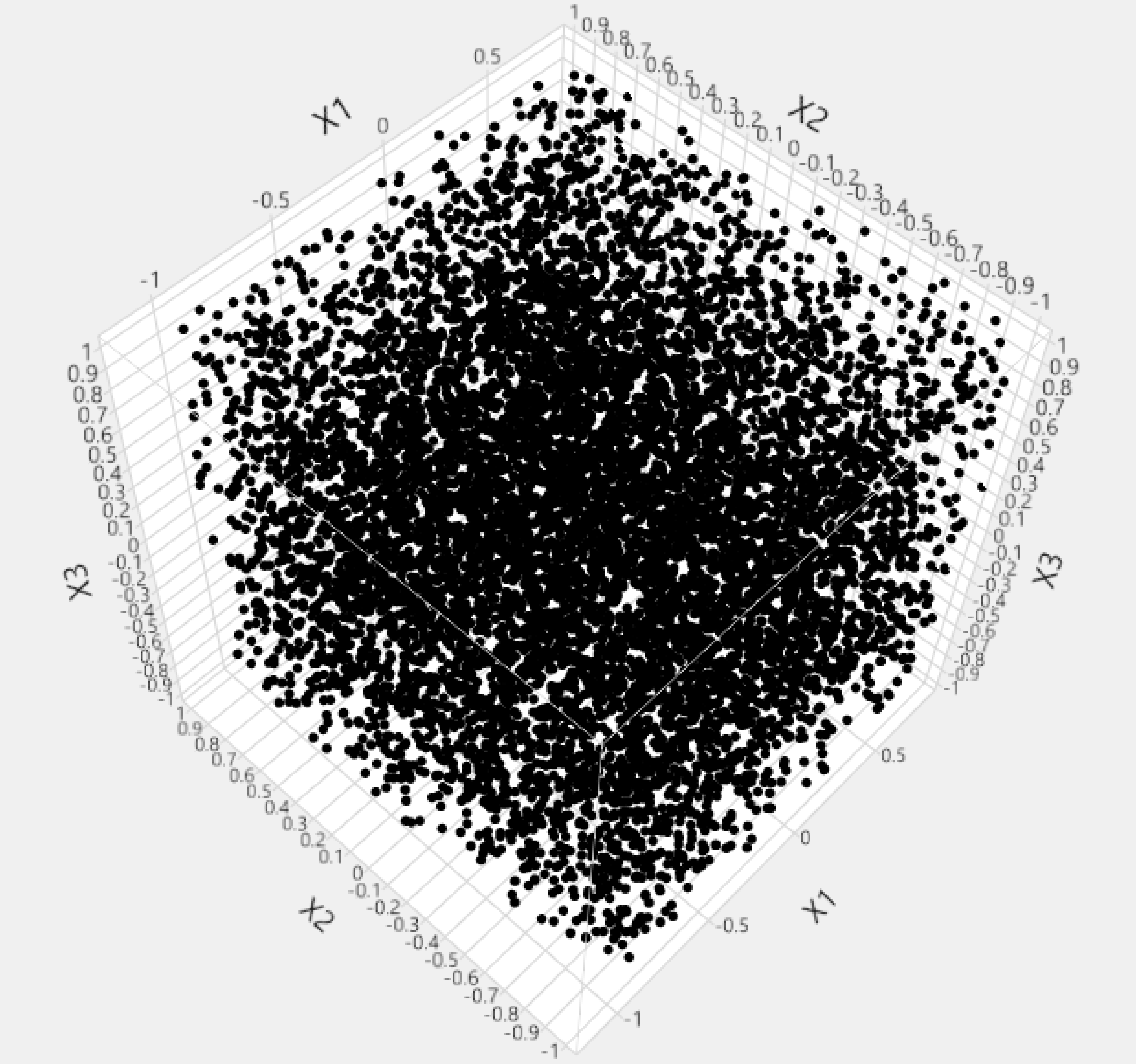
We calculate the RMSPE scores for all 1,000 $\mathbf{\hat{Y}}_{i}$’s for each model algorithm and noise level and present the results in Section 3.2. Due to extreme outlier RMSPE scores (in simulations mostly featuring the Fit Definitive Screening procedure) we made use of the log(RMSPE) metric instead. The RMSPE results can be found in the Appendx.

3.2 Simulation Results

For the DSDs in Figure 4 and 5 we see the obvious pattern emerge that SVEM model algorithms will perform better relative to their non-SVEM counterparts when there is less sparsity imposed in the true model. Conversely when A = 25% in both the $\sigma=1$ and $\sigma=3$ case we find a fair amount of overlap between all the model selection methods, however in every scenario we find the Fit Definitive Screening model to have higher RMSPE values. On balance we see that the SVEM methods performing consistently between the three versions with the Forward Selection implementation performing the best overall.

Interestingly enough we see that when $\sigma=1$ (see Figure 10) the Lasso and DS are the best performing non-SVEM models in the A = 25% case, but as the sparsity declines toward A = 100% we find they underperform even the forward selection and pruned forward selection models. Overall in all $\sigma=1$ cases (Figure 4) SVEM with forward regression has the lowest median log(RMSPE) score. What is further intriguing is when $\sigma=3$ (Figure 5) we also find the Lasso and DS models to outperform the non-SVEM models and are competitive with even the SVEM model algorithms. However, contrary to the $\sigma=1$ trend we find the Lasso and DS outperform the non-SVEM models, in Figure 5, as the sparsity declines toward A = 100%. In the same Figure 5 We even find the Lasso and DS to have the lowest median log(RMSPE) scores when A = 25% for K = 4. In every other simulation case, whilst the Lasso and DS are quite competitive when the sparsity is low, that SVEM with forward regression and SVEM with Lasso have the lowest median log(RMSPE) scores.

The the BBD simulation results presented in Figures 6 and 7 show a similar trend to the DSD results but the performance of the SVEM model algorithms are not as appreciable barring the forward selection and pruned forward selection which both under perform all other model algorithms in every scenario. We remind the reader that in the BBD simulations each design has $N>P$ i.e. none of the model matrices were super-saturated (like the DSD with K = 8) or saturated (like the DSD with K = 4). In Figure 6 where $\sigma=1$ the SVEM results are only slightly better than the Lasso and DS when A = 100% for both K = 3 and K = 5. When A = 25% and 50% we see no appreciable difference between SVEM and the Lasso and DS.

In Figure 7 where $\sigma=3$ we notice much of the same trends as in Figure 6 where the SVEM models have slightly improved median log(RMSPE) scores compared to the Lasso and the DS whereas the forward selection and pruned forward selection model algorithms have the highest log(RMSPE) scores in all cases. In all other sparsity scenarios (Figure 7) for both K = 3 and K = 5 we only notice one case (A = 25% and K = 3) where the Lasso and DS have slightly lower median log(RMSPE) score’s than all other model algorithms most notably the SVEM model algorithms, particularly SVEM with forward selection and SVEM with Lasso, which are in a close second position.

What we immediately deduce from these simulations is that SVEM outperforms its non SVEM counterparts when the true model has very low sparsity. The results become even more apparent when $P\approx N$ or $P>N$ or when smaller designs are used as seen in Figures 4 and 5. We further see this trend exacerbated when we increase the signal to noise ratio. The difference can be seen when comparing the $\sigma=1$ to the $\sigma=3$ results in Figure 4 and 5 respectively. Even when $N>P$ and $\sigma=3$ we find an appreciable improvement in median log(RMSPE) scores (Figure 7). When sparsity is high we see no reason not to use SVEM since the results are on par with the best non-SVEM model, which is usually the Lasso and or the DS.

We also find that in all of the nBoot = 200 runs within SVEM and through all the model selection algorithms in our simulations that most often SVEM will have $p\prime=P$ (Figures 8, 9, 10, and 11). Even in the case of the simulations with a DSD with $K=8$ (Figures 8, 9) we find this to be true even though $P=45$ and $N=21$. SVEM therefore produces a final model with the number of total selected effects exceeds the degrees of freedom available to us in the majority of DoEs increasing fitted model complexity, but subsequently improving predictive ability. In the case of the BBD simulations (Figures 10 and 11) we find the non-SVEM models sometimes yield the maximum model size such as the Lasso and DS in the $K=5$ and A = ALL scenarios, however the median model size for the non-SVEM model algorithms is clearly much lower than this upper bound. This is despite the fact that the BBDs have more than enough degrees of freedom ($P<N$) to select all predictors.

Even though the final model sizes for SVEM models appear to be large it is important to note that the some of the individual coefficients might be quite small. In Figure 12 we display the distributions of the coefficients for each predictor from a single simulation run in the DSD $K=4$, A = ALL, and $\sigma=3$ scenario. In this example we have $P\approx N$ and a model matrix with every predictor having a non-zero coefficient value. All 14 predictors are selected at least once and the coefficient had a non-zero value in every nBoot run. Some predictors have been selected far more than others ($X_{1},X_{4},X_{1}X_{2},X_{1}X_{3}$) whilst the majority fall into the category of moderate to slight rate of selection. This is similar to the discussion Burnham and Anderson, (2002) present regarding predictors not having binary contribution to a model but rather all predictors having at least some effect size albeit some will have an effect size near zero ($X_{4}X_{4}$).

Figure 4: DSD log(RMSPE) simulation results when $\sigma=1$

Figure 5: DSD log(RMSPE) simulation results when $\sigma=3$

Figure 6: BBD log(RMSPE) simulation results when $\sigma=1$

Figure 7: BBD log(RMSPE) simulation results when $\sigma=3$

Figure 8: DSD simulation model size results when $\sigma=1$

Figure 9: DSD simulation model size results when $\sigma=3$

Figure 10: BBD simulation model size results when $\sigma=1$

Figure 11: BBD simulation model size results when $\sigma=3$

Figure 12: Distributions of coefficients from a single DSD (K = 4, A = 100%, $\sigma=3$) Simulation using FWD with SVEM and nBoot = 200. The black vertical line represents the true model coefficient value and the red line represents the final SVEM coefficient value.

We ran another simulation to address the issue of an optimal number for the nBoot hyperparameter. The goal of this simulation is to discover a feasible value for nBoot. We used a DSD with $K=8$, A = ALL, and $\sigma=3$. We utilized the same FQ model as in the previous simulations (Figures 4, 5, 6 and 7) and we present the results with the RMSPE metric for 1,000 iterations using the SFD method used for the simulations above (see Section 3.1). We only made use of one model algorithm: SVEM with forward selection since it had the best performance on average in the previous simulations (See Section 3.2). We iterated the models over 5 values of nBoot: 1, 50, 100, 200, 500, 1000, 2000, and 3000.

Figure 13: Simulation results using SVEM with forward selection on a DSD with $K=8$, A = 100% and $\sigma=3$. The simulation was iterated over the hyperparameter nBoot to calculate a feasible value for SVEM. The horizontal red line represents the minimum median RMSPE score which corresponds to a nBoot = 500

There is clearly an improvement in the performance of SVEM when we increase nBoot from 1 to 50 and a further slight improvement in median log(RMSPE) scores when we increase nBoot from 50 to 100 (see Figure 13). The implication is that bagging is a key element in SVEM since no bagging is taking place when nBoot = 1, since there is only one model in $\mathbf{M}$. We do not see a significant improvement by increasing nBoot from 200 although there is a minor improvement from 200 to 1000 with the lowest median RMSPE score being nBoot = 500 (refer to the red horizontal line in Figure 13). We can deduce from this that an nBoot of 200 should be sufficient, in general, with an upper limit of 500. A user may wish to employ more nBoot runs, but there is unlikely to be an appreciable improvement in SVEM’s performance.

4 A Case Study: Plasmid Manufacturing

4.1 Overview

Plasmids (or pDNA) are non-chromosomal, circular shaped DNA found in the cells of various types of bacteria (e.g., E.coli). Plasmids are a key component in many new, biologic-based, cell and gene therapeutics, resulting in an increased demand for high-quality plasmids. However, plasmid manufacturing is challenging and demand for plasmids consistently exceeds the available supply (Xenopoulos and Pattnaik,, 2014).

4.2 Experimental Design and Models

In this case study a 5-factor, 15-run DSD was used to study the fermentation step of a plasmid manufacturing process. The goal of the experiment is to build a predictive model that is subsequently used to characterize and optimize a fermentation step of the plasmid manufacturing process. In addition, a separate 5-factor, 31-run central composite design (CCD) was performed. The experiment based on the CCD was performed independently of the DSD experiment in order to provide an independent assessment of the DSD predictive model performance. Tables 4 and 5 display the data for the two experiments; note that generic settings of the 5 factors are presented because the actual settings are proprietary. However, the values of the response, pDNA Titer mg/L (Yield), are the actual values observed.

The case study first illustrates the use of SVEM to build a predictive model for pDNA Titer based on data from the DSD study, and then applies this predictive model to the data from the CCD study in order to obtain an independent assessment of prediction performance on a true test set.

4.3 Results and Discussion

For this case study we compare predictions made from the DSD and consider the CCD to be the “true” values. We measure RMSPE on the models constructed on the DSD and the RMPSE from those models applied to the CCD points. We compare SVEM using Forward Selection and Lasso to classical “one-shot” approaches using both BIC and AICc with Forward Selection, and Lasso; Lasso with AICc was dropped as Lasso resulted in an intercept only model, which neither predicts well nor serves any value for the study. In addition the p-value based Fit Definitive method of Jones and Nachtsheim, (2017) was applied to the DSD data for model selection. In all cases, FQ models only were considered.

Criterion	Model Selection	Full Model (p = 20)	RMSPE DSD	RMSPE CCD	$\mathbf{R^{2}}$ CCD
SVEM*	Forward Selection	FQ	15.7	53.5	0.55
SVEM*	Lasso	FQ	14.8	57.8	0.45
BIC	Lasso	FQ	16.0	61.4	0.44
AICc	Forward Selection	FQ	29.4	71.5	0.50
P-Values	Fit Definitive	FQ	40.0	64.8	0.35
BIC	Forward Selection	FQ	16.5	76.4	0.46

Table 3: *NBoot = 1,000

Table 3 displays the results of the analyses in terms of RMSPE and $R^{2}$ on the CCD data. Predicted by Actual plots for some of the models in Table 3 are displayed in Figure 14. The actual by predicted plot for the best performing model algorithm (SVEM with Forward Selection) is displayed in Figure 14. The smallest test set RMPSE values were achieved with the SVEM-based methods. From Table 3 we find that SVEM with Forward Selection achieved the smallest RMPSE = 53.5 while second best results were for SVEM with Forward Selection achieved an RMPSE = 53.5. All the non-SVEM methods had test set RMPSE values $>$ 60.0. The worst performers in terms of test set RMPSE were Forward Selection with AICc, Fit Definitive, and Forward Selection with BIC (see Table 3). As mentioned the Lasso with AICc criterion resulted in an intercept only model despite searching for an optimal $\lambda$ (Lasso shrinkage parameter) over a 1,500 point grid on a square root scale and a log scale.

Figure 14: Actual by Predicted Plot. The CCD pDNA values plotted against the predicted pDNA values from the four best performing model algorithms.

Often, a study’s goal is to characterize the entire design region with the intent on scaling up a process. In these cases, the larger SVEM models are preferred for two reasons: they have the capacity to deal with the complexity over the entire experimental region, and the ability to accommodate the increased process complexity often encountered in scale up activities.

5 Concluding Remarks

In this paper we have proposed a general method that allows for machine learning ensemble modeling in small $N$ situations typical of designed experiments. We demonstrated via simulations and a case study, in Section 3 and Section 4 respectively, that the use of SVEM leads to lower average prediction error on independent test sets when compared to its non-SVEM counterparts in cases of low sparsity and when the signal to noise ratio is large. Most notably we see improvements in prediction variance for the supersaturated model matrices due to smaller designs and where $P>N$. SVEM is very general in its approach, and can possibly be applied to any designed experiment. One potential future investigation could be to apply SVEM in combination with ML models, like neural networks, to observational data where holdout cross-validation is typically applied.

SVEM makes minimal model building assumptions which are typically associated with statistical models: i.i.d normally distributed errors and $p\prime<N-1$ (Hastie et al.,, 2001) are not required by SVEM. We suspect the reason for SVEM’s improved performance over its non-SVEM counterparts relates to its ability to fit a supersaturated model via the ensembling procedure. It also overcomes the instability problem discussed by Breiman, (1996). This goes against the common convention that parsimonious models are desirable. SVEM shows us that we may gain greater accuracy by having more predictors in our models and not fewer (Smucker et al.,, 2020). Neal, (1996) claims that sometimes simple models will outperform more complex models, but deliberately limiting the complexity of a model is not fruitful when the problem is evidently complex.

SVEM has opened the door to a wide array of related research topics. First and foremost is the issue of quantification of the uncertainty around the predictions. Finding a way to not only calculate prediction intervals but to potentially improve their accuracy against the traditional regression prediction interval from the single pass through models can lead to important results for industrial DoE typically. This improved predictive accuracy does come at a cost. If the underlying model algorithm is computationally demanding like best subsets or a support vector machine then the computation time for SVEM and say 200 nBoot runs will be rather demanding on time and computational requirements.

Another important question is the implications for how designs are chosen and evaluated. Most designs are selected based on the assumption of effect sparsity (Hastie et al.,, 2001), especially in higher order interactions. Because all power and sample size studies assume that $P<N$ new approaches for evaluating designs prior to data collection may be needed. In principal, because SVEM has no distribution or degrees of freedom assumptions imposed, SVEM can be combined with non-normal response distributions, as well as more general machine learning model classes, such as neural networks, support vector machines, tree based algorithms etc. It is also not yet known how well SVEM will work in the case of randomization restrictions where there are blocking or whole plot factors, or whether SVEM will need to be generalized to accommodate these structures.

6 Appendix

Figure 15: DSD RMSPE results when $\sigma=1$

Figure 16: DSD RMSPE results when $\sigma=3$

Figure 17: BBD RMSPE results when $\sigma=1$

Figure 18: BBD RMSPE results when $\sigma=3$

pH	%DO	Induction Temperature    (Celsius)	Feed Rate	Induction    OD600	Titer mg/L
1	1	-1	1	-1	581.36
-1	-1	-1	1	-1	519.80
-1	1	-1	-1	-1	115.40
-1	1	-1	1	1	407.22
1	1	-1	-1	1	56.18
1	-1	1	1	-1	260.82
-1	-1	-1	-1	1	94.95
1	-1	-1	-1	-1	215.03
-1	1	1	-1	1	211.00
0	0	0	0	0	321.00
0	0	0	0	0	387.35
-1	1	1	1	-1	231.00
1	1	1	1	1	351.00
1	-1	-1	1	1	284.00
-1	-1	1	1	1	298.00
-1	-1	1	-1	-1	191.00
1	-1	1	-1	1	183.02
0	0	0	0	0	368.74
1	1	1	-1	-1	111.46
0	0	0	0	0	391.74
0	0	0	0	0	366.01
1.3	0	0	0	0	257.88
-1.3	0	0	0	0	295.68
0	1.3	0	0	0	385.54
0	-1.3	0	0	0	371.02
0	0	1.3	0	0	326.70
0	0	-1.3	0	0	251.76
0	0	0	1.3	0	351.11
0	0	0	-1.3	0	167.39
0	0	0	0	1.3	219.64
0	0	0	0	-1.3	239.29

Table 4: CCD for the pDNA yield study.

pH	%DO	Induction Temperature    (Celsius)	Feed Rate	Induction    OD600	Titer mg/L
0	1	1	-1	-1	156.20
0	-1	-1	1	1	318.45
1	0	-1	-1	1	398.00
-1	0	1	1	-1	285.60
1	-1	0	1	-1	229.00
-1	1	0	-1	1	377.00
1	-1	1	0	1	290.00
-1	1	-1	0	-1	123.00
1	1	1	1	0	299.00
-1	-1	-1	-1	0	428.00
0	0	0	0	0	327.80
0	0	0	0	0	339.74
0	0	0	0	0	387.35
0	0	0	0	0	393.97
0	0	0	0	0	348.08

Table 5: DSD for the pDNA yield study.

References

- Belkin et al., (2019) Belkin, M., Hsu, D., Ma, S., and Mandal, S. (2019). Reconciling modern machine-learning practice and the classical bias-variance trade-off. PNAS, 1116(32):15849 – 15854.
- Bose and Chatterjee, (2018) Bose, A. and Chatterjee, S. (2018). U-Statistics, -Estimators and Resampling. Springer, New York.
- Box and Behnken, (1960) Box, G. and Behnken, D. (1960). Some new three level designs for the study of quantitative variables. Technometrics, 2:455–475.
- Box and Wilson, (1951) Box, G. E. P. and Wilson, K. B. (1951). On the experimental attainment of optimum conditions. Journal of the Royal Statistical Society, Series B, 13:1–45.
- Breiman, (1994) Breiman, L. (1994). Bagging predictors. Journal of Times Series Analysis, 17.
- Breiman, (1996) Breiman, L. (1996). Heuristics of instability and stabilization in model selection. The Annals of Statistics, 24(6):2350–2383.
- Burnham and Anderson, (2002) Burnham, K. P. and Anderson, D. R. (2002). Model Selection and Multimodel Inference - 2nd ed. Springer-Verlag.
- Candes and Tao, (2007) Candes, E. and Tao, T. (2007). The dantzig selector: Statistical estimation when p is much larger than n. Annals of Statistics, 35(6):2392–2404.
- Chatterjee and Bose, (2005) Chatterjee, S. and Bose, A. (2005). Generalized boostrap for estimating equations. annals of statistics. Annals of Statistics, 33(2):414–436.
- Efron, (1979) Efron, B. (1979). Bootstrap methods: Another look at the jacknife. Annals of Statistics, 7(1):1–26.
- Efron and Tibshirani, (1993) Efron, B. and Tibshirani, R. (1993). An Introduction to the Bootstrap. Chapman and Hall/CRC, New York.
- Hastie et al., (2001) Hastie, T. J., Tibshirani, R. J., and Friedman, J. H. (2001). The Elements of Statistical Learning: Data Mining, Inference and Prediction. Springer.
- James et al., (2015) James, G. M., Witten, D., Hastie, T. J., and Tibshirani, R. J. (2015). Introduction to Statistical Learning 2nd ed. Springer, New York.
- Jones and Nachtsheim, (2011) Jones, B. and Nachtsheim, C. (2011). A class of three-level designs for definitive screening in the presence of second-order effects. Journal of Quality Tecnhology, 43(1).
- Jones and Nachtsheim, (2017) Jones, B. and Nachtsheim, C. (2017). Effective design-based model selection for definitive screening designs. Technometrics, 59(2):319–329.
- Marley and Woods, (2010) Marley, C. J. and Woods, D. C. (2010). A comparison of design and model selection methods for supersaturated experiments. Computational Statistics & Data Analysis, 54(12):3158–3167.
- Meinshausen et al., (2007) Meinshausen, N., Rocha, G., and Yu, B. (2007). Discussion: A tale of three cousins: Lasso, l2boosting and dantzig. Annals of Statistics, 35(6):2373–2384.
- Neal, (1996) Neal, R. (1996). Bayesian Learning for Neural Networks. Springer Science+Business Media, New York.
- Roshan, (2016) Roshan, V. J. (2016). Space-filling designs for computer experiments: A review. Quality Engineering, 28(1):28–35.
- Rubin, (1981) Rubin, D. (1981). The Bayesian bootstrap. Annals of Statistics, 9(1):130–134.
- SAS, (2020) SAS (2020). Jmp (version 16).
- Shmueli, (2010) Shmueli, G. (2010). To explain or predict. Statistical Science, 25(3):289–310.
- Smucker et al., (2020) Smucker, B., Edwards, D., and Weese, M. (2020). Response surface models: To reduce or not to reduce. JQT, 52(32).
- Tibshirani, (2014) Tibshirani, R. J. (2014). In praise of sparsity and convexity. Statistical Science, page 505–513.
- Xenopoulos and Pattnaik, (2014) Xenopoulos, A. and Pattnaik, P. (2014). Production and purification of plasmid dna vaccines: Is there scope for further innovation? Expert Review of Vaccines, 13(12).
- Xu et al., (2020) Xu, L., Gotwalt, C., Hong, Y., King, C., and Meeker, W. (2020). Applications of the fractional-random-weight bootstrap. The American Statistician, 74(4):1–29.
- Yuan et al., (2007) Yuan, M., Joseph, R., and Lin, Y. (2007). An efficient variable selection approach for analyzing designed experiments. Technometrics, 48(4):430–439.
- Yuan et al., (2009) Yuan, M., Roshan, V. J., and Hui, Z. (2009). Structured variable selection and estimation. The Annals of Statistics, pages 1738–1757.