Estimation of parameters of the logistic exponential distribution under progressive type-I hybrid censored sample*

Abstract

The present paper addresses the problem of estimation of the model parameters of the logistic exponential distribution based on progressive type-I hybrid censored sample. The maximum likelihood estimates are obtained and computed numerically using Newton-Raphson algorithm. Further, the Bayes estimates are derived under the squared error, LINEX and the generalized entropy loss functions. Two types (independent and bivariate) of prior distributions are considered for the purpose of Bayesian estimation. It is seen that the Bayes estimates are not of explicit forms. Thus, Lindley’s approximation technique is employed to get approximate Bayes estimates. Interval estimates of the parameters based on the normal approximation of the maximum likelihood estimates and the log-transformed maximum likelihood estimates are constructed. The highest posterior density credible intervals are obtained by using the importance sampling method. Numerical simulation is performed to see the performance of the proposed estimation techniques. A real life data set is considered and analysed for the purpose of illustrations.

Keywords: Newton-Raphson method; Independent and bivariate priors; Lindley’s approximation; Importance sampling method; Mean squared error; Coverage probability.

2010 Mathematics Subject Classification: 62N02; 62F10; 62F15

1 Introduction

Censoring was introduced in practice to save time and to reduce the number of failed units associated with a life-testing experiment. The concept of censoring is very common in reliability and survival studies. The type-I and type-II censoring schemes are two fundamental censoring schemes among all the schemes, developed so far. Suppose that $n$ units are placed to conduct a life-testing experiment. In type-I censoring scheme, it is assumed that the experiment runs up to a prefixed time, say $T$. Here, the random number of failures, say $m~(<n)$ in the time interval $[0,T]$ is observed. For the case of type-II censoring scheme, the experiment continues till a predefined number of failures, say $m$. Thus, clearly the time, say $T$ at which the experiment stops is random. Epstein 1954 introduced a censoring scheme by mixing type-I and type-II schemes, which is dubbed as the hybrid censoring scheme. The main drawback of the hybrid censoring scheme is that it does not have flexibility of removing experimental units before the experiment stops. However, the progressive type-II censoring scheme has such flexibility. Due to this virtue, the progressive type-II censoring design has been widely utilized to analyse lifetime data. But, these days, the system-components are highly reliable. This leads to a large experimental duration in progressive type-II censoring scheme. To overcome such difficulty, Kundu and Joarder 2006 introduced a general censoring scheme, known as the progressive type-I hybrid censoring scheme (PT-IHCS). Note that the PT-IHCS is a mixture of the hybrid and the progressive type-II censoring schemes, which is described in the following.

Suppose an experiment has been conducted with $n$ components. The random lifetimes of $n$ components are denoted by $X_{1},\ldots,X_{n}.$ Let an integer $m~(<n)$ and the time point $T$ be fixed when the experiment starts. At the time of first failure, say $X_{1:m:n}$, $R_{1}$ number of live units are randomly taken out. When the second failure occurs at $X_{2:m:n}$, $R_{2}$ units are removed from the experiment. Similarly, for the third failure, fourth failure and so on. Thus, two cases arise as follows. Assume that the $m$th failure occurs at time $X_{m:m:n}$, which is less than $T$. Then, the experiment stops at $X_{m:m:n}$. Other ways, let the $m$th failure occur after the time point $T$. The $j~(0\leq j<m)$ number of failures occur before $T$. Then, at $T$, the remaining units $R^{*}_{j}=n-R_{1}-R_{2}-.....-R_{j}-j$ are removed and the experiment terminates. These two cases are named as Case-$A$ and Case-$B$, which are presented below. This censoring scheme is known as the PT-IHCS. For details on this censoring design, one may refer to Kundu and Joarder 2006. Note that for the progressive type-I hybrid censored sample, one has either Case-$A$ or Case-$B$, where

Case-A $$: \{X_{1:m:n},\ldots,X_{m:m:n}\},~~\mbox{if}~~X_{m:m:n}<T;$$

Case-B $$: \{X_{1:m:n},\ldots,X_{j:m:n}\},~~~\mbox{if}~~X_{j:m:n}<T<X_{j+1:m:n}.$$

The meaning of $X_{j:m:n}<T<X_{j+1:m:n}$ is that the $j$th failure occurs before $T$, and no failure occurs between the points $X_{j:m:m}$ and $T$. That is, $X_{j+1:m:n},\ldots,X_{m:m:n}$ are not observed. Due to the importance of PT-IHCS, many authors have studied estimation of the parameters of various lifetime distributions based on this scheme. Lin et al. 2009 obtained some useful classical estimates of the unknown parameters of Weibull distribution under the PT-IHCS. The authors obtained maximum likelihood estimates (MLEs) and approximate MLEs. Hemmati and Khorram 2013 obtained various estimates for the log-normal distribution under progressive type-I hybrid censored (PT-IHC) sample. Sultana et al. 2019 studied estimation of parameters of the generalized half-normal distribution based on the PT-IHCS. They obtained maximum likelihood and Bayes estimates. Further, the authors computed Bayes estimates using different approximation techniques. Gamchi et al. 2019 considered classical and Bayesian inference of the Burr type-III distribution based on the PT-IHC data. One may refer to Kayal et al. 2019, Goyal et al. 2020, Sultana et al. 2020 and among others for some recent developments in this topic.

Figure 1: Plot of the hazard rate function of LE distribution with various combinations of parameters.

Let $X$ be a random variable following logistic exponential (LE) distribution (see Lan and Leemis 2008) with probability density function (PDF) $f$ and cumulative distribution function (CDF) $F$, where

$$f(x)\equiv f(x;\alpha,\lambda)=\frac{\alpha\lambda e^{\lambda x}(e^{\lambda x}-1)^{\alpha-1}}{\left[1+\left(e^{\lambda x}-1\right)^{\alpha}\right]^{2}};~x>0,~\alpha,~\lambda>0$$ (1.1)

and

$$F(x)\equiv F(x;\alpha,\lambda)=1-\left[1+(e^{\lambda x}-1)^{\alpha}\right]^{-1};~x>0,~\alpha,~\lambda>0.$$ (1.2)

Note that the LE distribution is a generalization of the exponential distribution. The CDF in (1.2) reduces to the CDF of exponential distribution when $\alpha=1$. The hazard rate function of the LE distribution is given by

$$h(x)\equiv h(x;\alpha,\lambda)=\frac{\alpha\lambda e^{\lambda x}(e^{\lambda x}-1)^{\alpha-1}}{1+\left(e^{\lambda x}-1\right)^{\alpha}};~x>0,~\alpha,~\lambda>0.$$ (1.3)

It becomes constant when $\alpha=1$, that is, it belongs to both increasing hazard rate and decreasing hazard rate classes. The LE distribution with CDF (1.2) has increasing and decreasing shaped hazard rate when $\alpha,~\lambda>1$. Further, the shape of the hazard rate function of this distribution is bathtub (upside down bathtub) when $0<\alpha<1$ ($\alpha>1$). Please refer to Lan and Leemis 2008 for various other properties of this distribution. It is worth mentioning that the LE distribution is the only two-parameter family of distributions that has five types of shapes of the hazard rate function. Figure $1$ depicts the graph of the hazard rate function of the LE distribution for various combinations of the parameters.

We recall that in reliability engineering, biology and several statistical modelings, different-shaped hazard rate functions are used with different interpretations. Consider a high failure rate during infancy, which decreases to a certain level, then it remains constant up to a certain time, and then it increases due to aging. This type of situation can be described by a bathtub-shaped hazard rate model. The data set on hydrodynamical devices (see Hjorth 1980) can be modeled using a statistical distribution having bathtub-shaped hazard rate. The decreasing hazard rate is usually observed in early stage of a working system. Data set on the earthquakes in North Anatolia fault zone can be fitted by a decreasing hazard model (see Kuş 2007). Further, increasing hazard rate models are used in operations and supply chain management research due to implications in evaluation of some type of objective functions to model stochastic events. In biology, it is observed in the course of a disease whose mortality reaches a peak after some finite period and then declines gradually. Thus, the data set related to this can be modeled using upside down bathtub-shaped hazard rate model. It is already mentioned before that the LE distribution exhibits the constant, increasing, decreasing, bathtub and upside down bathtub-shaped hazard rate. Due to various shapes of the hazard rate function, the LE distribution is very flexible to use in different areas of research such as clinical, reliability and survival studies. Due to wide practical utility of the LE distribution, we consider the problem of estimation of the model parameters problem with the importance of the PT-IHCS motivate us to consider the present estimation problem, since this problem has not been reported earlier in the literature.

First, we consider the MLEs of the unknown parameters based on the PT-IHC data from the LE distribution. The MLEs can not be obtained explicitly. Thus, Newton-Raphson iterative method is used to solve non-linear equations. Although, the performance of the MLEs is satisfactory, another way to estimate the parameters is Bayesian estimation. For Bayesian estimation, we need to choose prior distributions on the unknown model parameters. In this paper, the independent as well as bivariate priors have been considered. As expected, the explicit expressions of the Bayes estimates can not be obtained in explicit forms. Thus, we propose to use Lindley’s approximation method to compute the Bayes estimates. The importance sampling method is also used to compute the Bayes estimates and the highest posterior density (HPD) credible intervals. However, the values of the Bayes estimates using importance sampling method is not presented in the tables to maintain brevity. The approximate confidence intervals are also obtained using the asymptotic distribution of the MLEs. We consider a real life data set and analyzed it for the purpose of illustrations.

The paper is arranged as follows. In Section $2$, the MLEs of the parameters are computed using Newton-Raphson iterative method. To get rough idea on the existence and uniqueness of the MLEs, the plots of the profile log-likelihood function of the parameters are presented. The Bayes estimates are obtained using three loss functions. Two different types of the prior distributions are considered in this purpose. The form of the Bayes estimates are not of closed forms. Thus, Lindley’s approximation method is employed in Section $4$. Further, importance sampling method is utilized in order to construct HPD credible interval estimates. In Section $5$, two methods are used to compute asymptotic confidence intervals of the parameters. A simulation study is carried out in Section $6$ to observe the comparative performance of the proposed estimates. Section $7$ deals with a real life data set. Finally, in Section $8$, some concluding remarks are added.

2 Maximum likelihood estimation

This section focuses on the maximum likelihood estimation of the unknown model parameters $\alpha$ and $\lambda$ of the LE distribution with CDF (1.2) based on PT-IHC sample. Given the observed data, the likelihood function of $\alpha$ and $\lambda$ can be written as follows:

$$\mbox{Case-A :}~~~~~L(\alpha,\lambda) \propto \prod_{i=1}^{m}f(x_{i:m:n})[1-F(x_{i:m:n})]^{R_{i}},$$ (2.1)

$$\mbox{Case-B :}~~~~~L(\alpha,\lambda) \propto \prod_{i=1}^{j}f(x_{i:m:n})[1-F(x_{i:m:n})]^{R_{i}}[1-F(T)]^{R^{*}_{j}},$$ (2.2)

where $m~(\leq n)$ is a prefixed integer and $R^{*}_{j}=n-R_{1}-R_{2}-\ldots-R_{j}-j$. Henceforth, for notational convenience, $x_{i}$ is used for $x_{i:m:n}$. Eqs. $(\ref{eq2.1})$ and $(\ref{eq2.2})$ can be combined as

$$L(\alpha,\lambda)\propto\prod_{i=1}^{D}f(x_{i})[1-F(x_{i})]^{R_{i}}[1-F(T)]^{R^{*}_{D}},$$ (2.3)

where for Case-$A$, $D=m$, $R^{*}_{D}=0$, and for Case-$B$, $D=j$, $R^{*}_{D}=n-R_{1}-R_{2}-\ldots-R_{D}-D$. Denote $g(x;\lambda)=e^{\lambda x}-1,~x>0,~\lambda>0.$ Now, using (1.1) and (1.2), the likelihood function in (2.3) becomes

$$L(\alpha,\lambda)\propto\alpha^{D}\lambda^{D}e^{\lambda\sum_{i=1}^{D}x_{i}}\prod_{i=1}^{D}(g(x_{i};\lambda))^{\alpha-1}[1+(g(x_{i};\lambda))^{\alpha}]^{-(R_{i}+2)}[1+(g(T;\lambda))^{\alpha}]^{-R^{*}_{D}}.$$ (2.4)

Thus, the log-likelihood function is

$$\log L(\alpha,\lambda) = D\log\alpha+D\log\lambda+\lambda\sum_{i=1}^{D}x_{i}+(\alpha-1)\sum_{i=1}^{D}\log(g(x_{i};\lambda))$$ (2.5)

$$-\sum_{i=1}^{D}(R_{i}+2)\log[1+(g(x_{i};\lambda))^{\alpha}]-R^{*}_{D}\log[1+(g(T;\lambda))^{\alpha}].$$

Now, differentiating (2.5) with respect to $\alpha$ and $\lambda$, and equating to zero, the likelihood equations are respectively obtained as

$$\frac{\partial\log L}{\partial\alpha} = \frac{D}{\alpha}+\sum_{i=1}^{D}\log(g(x_{i};\lambda))-\sum_{i=1}^{D}\frac{(R_{i}+2)(g(x_{i};\lambda))^{\alpha}\log(g(x_{i};\lambda))}{[1+(g(x_{i};\lambda))^{\alpha}]}$$ (2.6)

$$-\frac{R^{*}_{D}(g(T;\lambda))^{\alpha}\log(g(T;\lambda))}{[1+(g(T;\lambda))^{\alpha}]}=0$$

and

$$\frac{\partial\log L}{\partial\lambda} = \frac{D}{\lambda}+\sum_{i=1}^{D}x_{i}+(\alpha-1)\sum_{i=1}^{D}\frac{x_{i}e^{\lambda x_{i}}}{g(x_{i};\lambda)}-\sum_{i=1}^{D}\frac{(R_{i}+2)\alpha x_{i}(g(x_{i};\lambda))^{\alpha-1}e^{\lambda x_{i}}}{[1+(g(x_{i};\lambda))^{\alpha}]}$$ (2.7)

$$-\frac{R^{*}_{D}\alpha T(g(T;\lambda))^{\alpha-1}e^{\lambda T}}{[1+(g(T;\lambda))^{\alpha}]}=0.$$

The MLEs of $\alpha$ and $\lambda$ are the solution of the simultaneous nonlinear equations given by (2.6) and (2.7). It is not easy to get solution of these equations in explicit form. So, Newton-Raphson (NR) iterative method is utilized to compute the MLEs of $\alpha$ and $\lambda$, which are respectively denoted by $\widehat{\alpha}$ and $\widehat{\lambda}$. Note that in order to apply NR method, ”nleqslv” package in R software has been used.

Figure 2: Profile log-likelihood function of $(a)$ $\alpha$ and $(b)$ $\lambda$, for the real dataset in Section $7$.

It is worth pointing that in statistical inference, it is always of interest to study the existence and uniqueness of the MLEs of the parameters. In order to achieve this, one requires to show two conditions proposed by Mäkeläinen et al. 1981. These are difficult to establish due to the complicated nature of the expressions of the second order partial derivatives of the log-likelihood function. However, to have a rough idea about the existence and uniqueness of the MLEs of $\alpha$ and $\lambda$ for the LE distribution under PT-IHC sample, the profile log-likelihood function for the parameters are presented in Figure $2.$ These plots show that the MLEs may exist uniquely. Note that the MLEs can be obtained efficiently using numerical approximation techniques. However, the exact distribution of the MLEs is hard to derive. As a result, the confidence intervals of the unknown model parameters are difficult to produce. The observed Fisher information matrix can be used to construct asymptotic confidence intervals of the parameters, which is discussed in Section $5$. Since it is not possible to derive the exact distribution of the MLEs, the natural choice is the Bayesian inference. This is presented in the next section.

3 Bayesian estimation

This section deals with the derivation of the Bayes estimates of the parameters $\alpha$ and $\lambda$ of the LE distribution with respect to three loss functions when PT-IHC sample is available. The squared error, LINEX and the generalized entropy loss functions are considered. Among these, the squared error loss function (SELF) is symmetric and other two are asymmetric. Let $\delta$ be an estimator of the parameter $\eta$. Then, the SELF is given by

$$L_{SQ}(\eta,\delta)=(\delta-\eta)^{2},$$ (3.1)

which assigns equal weight in underestimation as well as in overestimation. Sometimes, it is also called balanced loss function. There are various situations, where symmetric loss function is not an appropriate tool to use. For example, when estimating lifetime of a satellite, the overestimation is more serious than underestimation. Further, for estimating water level of a river in rainy season, the underestimation is more serious than overestimation. In these situations, the following loss functions, known as the LINEX loss (see Varian 1975) and generalized entropy loss (see Calabria and Pulcini 1994) are useful, respectively given by

$$L_{LI}(\eta,\delta) = e^{p(\delta-\eta)}-p(\delta-\eta)-1,~~p\neq 0;$$ (3.2)

$$L_{GE}(\eta,\delta) = \left(\frac{\delta}{\eta}\right)^{q}-q\log\left({\frac{\delta}{\eta}}\right)-1,~~q\neq 0.$$ (3.3)

Note that the sign of $p$ in the LINEX loss function represents the direction of asymmetry, and its magnitude reflects the degree of its asymmetry. For $p<0$, a negative error has a more serious effect, and for $p>0$ the effect of a positive error is more serious. Under the loss functions given by (3.1), (3.2) and (3.3), the Bayes estimates can be written in terms of the conditional expectations as

$$\widehat{\eta}_{SQ} = E_{\eta}(\eta|data);$$ (3.4)

$$\widehat{\eta}_{LI} = -p^{-1}\log[E_{\eta}(e^{-p\eta}|data)],~~p\neq 0;$$ (3.5)

$$\widehat{\eta}_{GE} = [E_{\eta}(\eta^{-q}|data)]^{-\frac{1}{q}},~~q\neq 0.$$ (3.6)

In Bayesian estimation, prior distribution has an important role. According to Arnold and Press 1983 there is no way, in which someone can say which prior is better than the other. They additionally stated that it is all the more regularly the case that somebody chooses to confine consideration regarding a given adaptable group of priors, and then picks one from that family which appears to be the best match with their own convictions. In this case, two different types of priors are considered and then, the Bayes estimates are derived.

3.1 Independent priors

We recall that when both the model parameters are unknown, no joint conjugate prior is available. For such situation, there are number of ways to consider the priors. For the present study, we consider independent gamma priors. This is due to the fact that the gamma distribution has a log-concave density function in the interval $(0,\infty)$ and Jeffery’s prior can be obtained as a special case of the gamma prior. Denote by $Gamma(a,b)$ for the gamma distribution with shape parameter $a$ and scale parameter $1/b$. Let $\alpha\sim Gamma(a,b)$ and $\lambda\sim Gamma(c,d)$. The PDFs of $\alpha$ and $\lambda$ are respectively given by

$$\pi_{1}(\alpha)\propto\alpha^{a-1}e^{-b\alpha}~~\mbox{and}~~\pi_{2}(\lambda)\propto\lambda^{c-1}e^{-d\lambda},$$ (3.7)

where $\alpha,~\lambda>0,~~a,~b,~c,~d>0$. The joint prior distribution of $\alpha$ and $\lambda$ is

$$\pi_{3}(\alpha,\lambda)\propto\alpha^{a-1}e^{-b\alpha}\lambda^{c-1}e^{-d\lambda};~\alpha,~\lambda>0,~~a,~b,~c,~d>0.$$ (3.8)

After some calculations, the posterior PDF of $\alpha$ and $\lambda$ given the observed data is obtained as

$$\pi(\alpha,\lambda|data) = k_{1}^{-1}\alpha^{D+a-1}\lambda^{D+c-1}e^{-b\alpha}e^{-\lambda(d-\sum_{i=1}^{D}x_{i})}\prod_{i=1}^{D}(g(x_{i};\lambda))^{\alpha-1}[1+(g(x_{i};\lambda))^{\alpha}]^{-(R_{i}+2)}$$ (3.9)

$$\times[1+(g(T;\lambda))^{\alpha}]^{-R^{*}_{D}},$$

where $k_{1}$ is given in $(\ref{A1})$. Now, consider a function of the parameters $\alpha$ and $\lambda$, say $\phi(\alpha,\lambda).$ Then, from (3.4), (3.5) and (3.6), the forms of the Bayes estimates of $\phi(\alpha,\lambda)$ with respect to the squared error, LINEX and the generalized entropy loss functions are given by

$$\widehat{\phi}_{SQ} = \int_{0}^{\infty}\int_{0}^{\infty}\phi(\alpha,\lambda)\pi(\alpha,\lambda|data)d\alpha d\lambda;$$ (3.10)

$$\widehat{\phi}_{LI} = -p^{-1}\log\left[\int_{0}^{\infty}\int_{0}^{\infty}\phi(\alpha,\lambda)\pi(\alpha,\lambda|data)d\alpha d\lambda\right],~~p\neq 0;$$ (3.11)

$$\widehat{\phi}_{GE} = \left[\int_{0}^{\infty}\int_{0}^{\infty}\left(\phi(\alpha,\lambda)\right)^{-q}\pi(\alpha,\lambda|data)d\alpha d\lambda\right]^{-\frac{1}{q}},~~q\neq 0,$$ (3.12)

respectively. Note that $(\ref{eq3.12})$ reduces to $(\ref{eq3.10})$, for $q=-1.$ To derive the Bayes estimates of $\alpha$ and $\lambda$ with respect to the loss functions given by (3.1), (3.2) and (3.3), one needs to replace $\phi(\alpha,\lambda)$ by $\alpha$ and $\lambda$, respectively in (3.10), (3.11) and (3.12). In the following, the form of the Bayes estimates of $\alpha$ with respect to the loss functions (3.1), (3.2) and (3.3) are respectively obtained as

$$\widehat{\alpha}_{SQ} = \int_{0}^{\infty}\int_{0}^{\infty}\alpha\pi(\alpha,\lambda|data)\ d\alpha d\lambda;$$ (3.13)

$$\widehat{\alpha}_{LI} = -p^{-1}\log\Bigg[\int_{0}^{\infty}\int_{0}^{\infty}\alpha\pi(\alpha,\lambda|data)d\alpha d\lambda\Bigg];$$ (3.14)

$$\widehat{\alpha}_{GE} = \Bigg[\int_{0}^{\infty}\int_{0}^{\infty}\alpha^{-q}\pi(\alpha,\lambda|data)d\alpha d\lambda\Bigg]^{-\frac{1}{q}}.$$ (3.15)

In analogy to $\widehat{\alpha}_{SQ}$, $\widehat{\alpha}_{LI}$ and $\widehat{\alpha}_{GE}$, the Bayes estimates of $\lambda$ under the loss functions (3.1), (3.2) and (3.3) can be obtained, which are denoted by $\widehat{\lambda}_{SQ}$, $\widehat{\lambda}_{LI}$ and $\widehat{\lambda}_{GE}$, respectively. These are omitted for the sake of conciseness.

3.2 Bivariate prior

In this subsection, let us consider a bivariate prior for $\alpha$ and $\lambda$, which is given by

$$\pi^{*}(\alpha,\lambda)=\pi_{1}^{*}(\alpha|\lambda)\pi_{2}(\lambda);~~\alpha>0,~\lambda>0.$$ (3.16)

where $\pi_{2}(\lambda)$ is given by (3.7) and

$$\pi_{1}^{*}(\alpha|\lambda)\propto\frac{1}{\lambda};~~\alpha>0,~\lambda>0.$$ (3.17)

The prior $\pi_{1}^{*}(\alpha|\lambda)$ is known as the noninformative prior of $\alpha$ when $\lambda$ is fixed. Thus, from (3.16), the bivariate prior distribution of $\alpha$ and $\lambda$ is given by

$$\pi^{*}(\alpha,\lambda)\propto{\lambda}^{(c-2)}e^{-d\lambda};~~\alpha,~\lambda>0,~~c,~d>0.$$ (3.18)

Similar to the preceding subsection, the posterior PDF of $\alpha$ and $\lambda$ given the observed data is obtained as

$$\pi_{2}^{*}(\alpha,\lambda|data) = k_{2}^{-1}\alpha^{D}\lambda^{D+c-2}e^{-\lambda(d-\sum_{i=1}^{D}x_{i})}\prod_{i=1}^{D}(g(x_{i};\lambda))^{\alpha-1}[1+(g(x_{i};\lambda))^{\alpha}]^{-(R_{i}+2)}$$ (3.19)

$$\times[1+(g(T;\lambda))^{\alpha}]^{-R^{*}_{D}},$$

where $k_{2}$ is given in $(\ref{A2})$. Based on the posterior density function given by (3.19), the Bayes estimates of the parameters $\alpha$ and $\lambda$ can be obtained with respect to the loss functions (3.1), (3.2) and (3.3). The expressions are omitted for the sake of brevity. Considering the bivariate prior distributions, the Bayes estimates of $\alpha$ under the loss functions (3.1), (3.2) and (3.3) are denoted by $\hat{\alpha}_{dSQ}$, $\hat{\alpha}_{dLI}$ and $\hat{\alpha}_{dGE}$, respectively. Further, the Bayes estimates of $\lambda$ under the loss functions (3.1), (3.2) and (3.3) are denoted by $\hat{\lambda}_{dSQ}$, $\hat{\lambda}_{dLI}$ and $\hat{\lambda}_{dGE}$, respectively.

4 Approximation techniques

There are various techniques in the literature which have been used to compute approximate Bayes estimates. In this section, two approaches are employed for the evaluation of the Bayes estimates obtained in the preceding section. First, consider Lindley’s method, which expresses how to approximate a ratio of two particular forms of integrations. For details, please refer to Lindley 1980.

4.1 Lindley’s approximation method

This subsection deals with the computation of the Bayes estimates of $\alpha$ and $\lambda$ of the LE distribution under the loss functions given by (3.1), (3.2) and (3.3) when PT-IHC sample is available. First, let us write the Bayes estimate of $\alpha$ with respect to the LINEX loss function. Please refer to Appendix B for the idea on Lindley’s approximation method. In this case, for $p\neq 0,$ one has

$$\phi(\alpha,\lambda)=e^{-p\alpha},~v_{1}=-pe^{-p\alpha},~v_{11}=p^{2}e^{-p\alpha},~v_{2}=v_{12}=v_{21}=v_{22}=0.$$

Thus, using $(\ref{a1})$, the approximate Bayes estimate of $\alpha$ under LINEX loss function is obtained as

$$\widehat{\alpha}_{LI} \approx -\left(\frac{1}{p}\right)\log\Big[e^{-p\alpha}+\frac{1}{2}\{p^{2}e^{-p\alpha}-pe^{-p\alpha}(l_{30}\tau^{2}_{11}+l_{03}\tau_{21}\tau_{22}+3l_{21}\tau_{11}\tau_{12}$$ (4.20)

$$+l_{12}(\tau_{11}\tau_{22}+2\tau^{2}_{21})+2P_{1}\tau_{11}+2P_{2}\tau_{21})\}\Big],$$

where the other unknown terms in (4.20) are given in Appendix B. Next, consider the general entropy loss function given by (3.3). Under this loss function,

$$\phi(\alpha,\lambda)=\alpha^{-q},~v_{1}=-q\alpha^{-(q+1)},~v_{2}=q(q+1)\alpha^{-(q+2)},~v_{2}=v_{12}=v_{21}=v_{22}=0.$$

Therefore, under the general entropy loss function, the approximate Bayes estimate of $\alpha$ can be obtained, which is given by

$$\widehat{\alpha}_{GE} \approx \Big[\alpha^{-q}+0.5\{q(q+1)\alpha^{-(q+2)}-q\alpha^{-(q+1)}(l_{30}\tau^{2}_{11}+l_{03}\tau_{21}\tau_{22}+3l_{21}\tau_{11}\tau_{12}$$ (4.21)

$$+l_{12}(\tau_{11}\tau_{22}+2\tau^{2}_{21})+2P_{1}\tau_{11}+2P_{2}\tau_{21})\}\Big]^{-\frac{1}{q}}.$$

Note that the Bayes estimate of $\alpha$ with respect to the SELF (denoted by $\widehat{\alpha}_{SQ}$) can be computed from (4.21) when $q=-1.$ The Bayes estimates of $\lambda$ with respect to the LINEX, generalized entropy and the squared error loss functions can be derived similarly, and therefore the expressions are omitted. The Bayes estimates of $\lambda$ with respect to the loss functions (3.1), (3.2) and (3.3) using Lindley’s approximation technique are denoted by $\widehat{\lambda}_{SQ}$, $\widehat{\lambda}_{LI}$ and $\widehat{\lambda}_{GE},$ respectively. Further, when the bivariate prior distribution for $\alpha$ and $\lambda$ (see Subsection $3.2$) is considered, the approximate Bayes estimates for $\alpha$ and $\lambda$ can be obtained similar to the case of independent priors. Some changes in computing $P_{1}$ and $P_{2}$ are required in this purpose.

4.2 Importance sampling method

In this subsection, importance sampling method is used to evaluate the Bayes estimates of the parameters $\alpha$ and $\lambda$ with respect to the squared error, LINEX and the generalized entropy loss functions. The main advantage of this method over the Lindley’s approximation method is that this method can be used to construct HPD credible intervals. In this method, one needs to rewrite the posterior PDF given by Equation (3.9) as

$$\pi(\alpha,\lambda|data)\propto G_{\lambda}\left(D+c,d-\sum_{i=1}^{D}x_{i}\right)G_{\alpha|\lambda}\left(D+a,b-\sum_{i=1}^{D}\log(g(x_{i};\lambda))\right)h(\alpha,\lambda),$$ (4.22)

where $G(a_{1},a_{2})$ represents gamma distribution with parameters $a_{1}$ and $a_{2}$, and $h(\alpha,\lambda)$ is given in $(\ref{A6})$.

Further, in Eq. (4.22), $G_{\lambda}\left(D+c,d-\sum_{i=1}^{D}x_{i}\right)$ and $G_{\alpha|\lambda}\left(D+a,b-\sum_{i=1}^{D}\log(g(x_{i};\lambda))\right)$ mean

$$\lambda\sim G\left(D+c,d-\sum_{i=1}^{D}x_{i}\right)~~\mbox{and}~~\alpha|\lambda\sim G\left(D+a,b-\sum_{i=1}^{D}\log(g(x_{i};\lambda))\right).$$

Now, the algorithm comprising of the following steps can be used to obtain Bayes estimates of $\phi(\alpha,\lambda)$ with respect to the loss functions given by (3.1), (3.2) and (3.3).
——————————————————————————————————————
Algorithm-1
——————————————————————————————————————

• Generate $\lambda$ from $G\left(D+c,d-\sum_{i=1}^{D}x_{i}\right)$ distribution.

• For the given value of $\lambda$ in Step-$1$, generate $\alpha$ from $G\left(D+a,b-\sum_{i=1}^{D}\log(g(x_{i};\lambda))\right)$ distribution.

• Repeat Step-1 and Step-2, for $N$ times to obtain $(\alpha_{1},\lambda_{1}),\ldots,(\alpha_{N},\lambda_{N}).$

——————————————————————————————————————-
Based on the values as in Step-3, the Bayes estimates of a parametric function $\phi(\alpha,\lambda)$ under the LINEX and the generalized entropy loss functions are obtained as

$$\tilde{\phi}_{LI}=-\left(\frac{1}{p}\right)\log\left[\frac{\sum_{i=1}^{N}e^{-p\phi(\alpha_{i},\lambda_{i})}h(\alpha_{i},\lambda_{i})}{\sum_{i=1}^{N}h(\alpha_{i},\lambda_{i})}\right]$$ (4.23)

and

$$\tilde{\phi}_{GE}=\left[\frac{\sum_{i=1}^{N}\phi^{-q}(\alpha_{i},\lambda_{i})h(\alpha_{i},\lambda_{i})}{\sum_{i=1}^{N}h(\alpha_{i},\lambda_{i})}\right]^{-\frac{1}{q}},$$ (4.24)

respectively. The Bayes estimate with respect to the SELF, denoted by $\tilde{\phi}_{SQ}$ can be obtained from (4.24) when $q=-1.$ Further, the Bayes estimates of $\alpha$ with respect to the loss functions (3.2) and (3.3) can be respectively obtained from (4.23) and (4.24) after substituting $\alpha_{i}$ in place of $\phi(\alpha_{i},\lambda_{i})$. Similarly, the Bayes estimates of $\lambda$ can be evaluated. The Bayes estimates of $\alpha$ (respectively $\lambda$) with respect to the loss functions given by (3.1), (3.2) and (3.3) obtained using importance sampling method are denoted by $\tilde{\alpha}_{SQ}$ (respectively $\tilde{\lambda}_{SQ}$), $\tilde{\alpha}_{LI}$ (respectively $\tilde{\lambda}_{LI}$) and $\tilde{\alpha}_{GE}$ (respectively $\tilde{\lambda}_{GE}$), respectively. It is known that the credible intervals are constructed based on the posterior distribution. Further, if the credible interval satisfies the condition of HPD interval, then it is called as the HPD credible interval. In this paper, the $100(1-\beta)\%$ HPD credible intervals of the parameters $\alpha$ and $\lambda$ are constructed numerically based on the generated posterior samples. In this context, the idea proposed by Chen and Shao 1999 has been used. Note that although the importance sampling method is used to compute Bayes estimates and then HPD credible intervals, the Bayes estimates using importance sampling method are not presented in Section $6$ for brevity.

5 Interval estimation

In this section, two methods are employed to construct confidence intervals of $\alpha$ and $\lambda.$ Using the asymptotic normality property of the MLEs $\widehat{\alpha}$ and $\widehat{\lambda}$, the $100(1-\beta)\%$ confidence intervals of the unknown model parameters $\alpha$ and $\lambda$ can be constructed. In doing so, the variances of $\widehat{\alpha}$ and $\widehat{\lambda}$ are required, which can be obtained from the inverse of the observed Fisher information matrix. Note that under some regularity conditions, the MLEs $(\widehat{\alpha},\widehat{\lambda})$ asymptotically follow bivariate normal distribution with mean vector $(\alpha,\lambda)$ and variance-covariance matrix $I^{-1}(\widehat{\alpha},\widehat{\lambda})$. That is,

$$(\widehat{\alpha},\widehat{\lambda})\sim N((\alpha,\lambda),\widehat{I}^{-1}(\widehat{\alpha},\widehat{\lambda})),$$

where $\widehat{I}(\widehat{\alpha},\widehat{\lambda})$ is the observed Fisher information matrix given by

$$\widehat{I}(\widehat{\alpha},\widehat{\lambda})={\begin{bmatrix}-l_{20}&-l_{11}\\ -l_{11}&-l_{02}\\ \end{bmatrix}}_{({\alpha},{\lambda})=(\widehat{\alpha},\widehat{\lambda})}.$$ (5.1)

The elements of the observed Fisher information matrix given by (5.1) are provided in Appendix B. Note that the variances of $\widehat{\alpha}$ and $\widehat{\lambda}$, respectively denoted by $Var(\widehat{\alpha})$ and $Var(\widehat{\lambda})$ can be obtained from the main diagonal entries of the matrix $\widehat{I}^{-1}(\widehat{\alpha},\widehat{\lambda}).$ Thus, the $100(1-\beta)\%$ approximate confidence intervals for $\alpha$ and $\lambda$ are constructed as

$$\left(\widehat{\alpha}\pm z_{\frac{\beta}{2}}\sqrt{Var(\widehat{\alpha})}\right)~~\mbox{ and}~~\left(\widehat{\lambda}\pm z_{\frac{\beta}{2}}\sqrt{Var(\widehat{\lambda})}\right),$$

where $z_{\beta/2}$ is the percentile of the standard normal distribution with right-tail probability $\beta/2$. In some cases, the $100(1-\beta)\%$ confidence interval has negative lower bound when the parameter takes positive value. This is a drawback of the normal approximation of the MLEs. To overcome this drawback, Meeker and Escobar 2014 introduced log-transformed MLE-based confidence intervals. According to these authors, the confidence interval obtained based on logarithm transformed MLEs has better coverage probability. Based on the log-transformed MLEs, the $100(1-\beta)\%$ confidence intervals of $\alpha$ and $\lambda$ are respectively given by

$$\left(\widehat{\alpha}\exp\left\{\pm\frac{z_{\frac{\beta}{2}}\sqrt{\tau_{11}}}{\widehat{\alpha}}\right\}\right)~~\mbox{and}~~\left(\widehat{\lambda}\exp\left\{\pm\frac{z_{\frac{\beta}{2}}\sqrt{\tau_{22}}}{\widehat{\lambda}}\right\}\right).$$

6 A simulation study

In this section, a Monte Carlo simulation is performed to investigate the performance of the proposed estimates for LE distribution under PT-IHC sample. The comparative performance of the point estimates is studied in terms of the average and mean squared error (MSE) values. The interval estimates are compared based on the average lengths. In doing so, $2000$ PT-IHC samples are generated using various censoring schemes. Several combinations of $(n,m)$ are considered. The values of $T$ are taken as $0.5$ and $0.65$. The $R~3.4.0$ software is used for the purpose of simulation. Two different (total) sample sizes $n=35$ and $40$ are considered here. The numerical study includes the following steps:

1. True values of the model parameters are assumed as $\alpha=1.5$ and $\lambda=0.75$.

2. The PT-IHC samples for different $n$ and $m$ have been generated. Here, the values of $(n,m)$ are considered as $(35,10)$, $(35,25)$, $(40,10)$ and $(40,30)$.

3. In the tables, ($0*3$) and ($1*5$) represent $(0,0,0)$ and $(1,1,1,1,1)$, respectively. For each censored schemes, average values of the MLEs and the Bayes estimates corresponding to the univariate and bivariate priors and the associated MSEs are tabulated in Tables 1, 2, 5 and 6. Note that the comparisons of the proposed estimates are made based on the average and MSE values. To compute MSE, the following formula is used:

   $$MSE=\frac{1}{M}\sum_{i=1}^{M}\left[\theta^{(i)}_{k}-\theta_{k}\right]^{2}; i=1,~2,$$

   where $\theta_{1}=\alpha$, $\theta_{2}=\lambda$ and $M=2000$.

4. The Bayes estimates of $\alpha$ and $\lambda$ are obtained with respect to the squared error loss function (SELF), LINEX loss function (LLF) and the generalized entropy loss function (GELF). In this purpose, the hyperparameters are considered as $a=3,~b=2,~c=3$ and $d=4$. We note that Lindley’s approximation method is used to compte the estimated values of the Bayes estimates. To obtain Bayes estimates under the LLF and the GELF, three choices of $p$ and $q$ are considered as $p=(-0.05,0.5,1)$ and $q=(-0.5,-0.25,0.25)$.

5. In Tables 3 and 7, the computed average lengths of $90\%$ and $95\%$ confidence intervals using normal approximation to MLEs (NA) and normal approximation to the log-transform MLEs (NL) methods are presented for $\alpha$ and $\lambda$. The average lengths of the HPD credible intervals of these parameters are also provided there. It is worth mentioning that the importance sampling method is utilized in order to get the HPD credible intervals since Lindley’s approximation technique can not be used to obtain the same.

In this part of the section, the coverage probabilities of the unknown parameters are discussed. To this aim, the asymptotic pivotal quantities are defined as

$$Q_{1}=\frac{\widehat{\alpha}-\alpha}{\widehat{\lambda}\sqrt{\tau_{11}}}, Q_{2}=\frac{\widehat{\alpha}-\alpha}{{\lambda}\sqrt{\tau_{11}}}, Q_{3}=\frac{\widehat{\lambda}-\lambda}{\widehat{\lambda}\sqrt{\tau_{22}}}.$$

By using Monte Carlo simulation, the coverage probabilities

$$P(-1.65\leq Q_{i}\leq 1.65)~~\mbox{and}~~P(-1.96\leq Q_{i}\leq 1.96)$$

for $i=1,~2,~3$ are computed, which are approximately $90\%$ and $95\%$, respectively (see Tables $4$ and $8$). From Tables $1$-$8$, the following observations have been made.

1. Under the same censoring schemes when $T$ increases, MSE decreases. Further, for fixed $n$, when $m$ increases, then MSE decreases.

2. For the parameter $\alpha$, in general, the Bayes estimates under GELF perform better than other estimates, whereas, for $\lambda$, most of the times, the Bayes estimates under LLF perform better than other estimates. To estimate $\alpha$, LLF performs better when $p=1$, and GELF perform better when $q=0.25$ and to estimate $\lambda$, LLF performs better when $p=-0.05$, and GELF performs better when $q=-0.5$. The Bayes estimates under SELF are almost equal to the value of the Bayes estimates under LLF when $p$ is nearly $0$. Further, the Bayes estimates under the univariate (U) prior perform better than the estimates with respect to the bivariate (B) priors in most of the cases.

3. When $T$ increases, length of the confidence intervals decrease. For each censoring schemes, the lengths of the NA-based confidence intervals are smaller than that of the NL-based confidence intervals.

4. The HPD credible interval lengths are smaller than other simulated interval lengths. Hence, HPD credible intervals perform better than other intervals.

5. The coverage probabilities of the above mentioned pivotal quantities $Q_{1}$, $Q_{2}$ and $Q_{3}$ increase when $m$ and $T$ both increase. Furthermore, coverage probabilities under $Q_{2}$ are much better than other two pivotal quantities.

Table 1: Average and MSE values of the estimates of $\alpha$ (true value=1.5) for $T=0.5$. The first (second) rows corresponding to ‘U’ and ‘B’ are for the average (MSE) values of the estimates.

(n,m)	scheme	prior	$\widehat{\alpha}$		$\widehat{\alpha}_{LI}$			$\widehat{\alpha}_{GE}$			$\widehat{\alpha}_{SQ}$
				$p=-0.05$	$p=0.5$	$p=1$	$q=-0.5$	$q=-0.25$	$q=0.25$
(35,10)	(0*9,25)	U	1.7716	1.6524	1.5913	1.5467	1.6142	1.5993	1.5721		1.6464
			0.0737	0.0232	0.0083	0.0022	0.0131	0.0099	0.0052		0.0214
		B		1.6626	1.5981	1.5483	1.6219	1.6054	1.5748		1.6565
				0.0264	0.0096	0.0023	0.0148	0.0112	0.0056		0.0245
	(0*5,5*5)	U	1.7555	1.5789	1.5335	1.5021	1.5502	1.5393	1.5199		1.5744
			0.0653	0.0062	0.0011	0.0004	0.0025	0.0015	0.0004		0.0055
		B		1.6092	1.5368	1.4785	1.5716	1.5374	1.5032		1.5937
				0.0119	0.0014	0.0005	0.0051	0.0014	0.0001		0.0087
	(25,0*9)	U	1.7059	1.5201	1.4763	1.4464	1.4917	1.4811	1.4623		1.5156
			0.0424	0.0004	0.0006	0.0028	0.0001	0.0004	0.0014		0.0002
		B		1.6431	1.5750	1.5239	1.5999	1.5828	1.5525		1.6365
				0.0204	0.0056	0.0006	0.0099	0.0068	0.0027		0.0186
(35,25)	(0*24,10)	U	1.7217	1.5265	1.4764	1.4429	1.4942	1.4451	1.4231		1.4874
			0.0491	0.0007	0.0005	0.0032	0.0000	0.0030	0.0059		0.0001
		B		1.6320	1.5751	1.5302	1.5933	1.5806	1.5527		1.6266
				0.0174	0.0056	0.0014	0.0087	0.0065	0.0027		0.0160
	(0*20,2*5)	U	1.6923	1.4860	1.4331	1.4248	1.4748	1.4628	1.4419		1.5015
			0.0369	0.0002	0.0044	0.0056	0.0006	0.0013	0.0033		0.0001
		B		1.6410	1.5833	1.5380	1.6041	1.5892	1.5611		1.6355
				0.0198	0.0069	0.0009	0.0108	0.0079	0.0037		0.0183
	(10,0*24)	U	1.6781	1.5209	1.4728	1.4388	1.4894	1.4773	1.4558		1.5161
			0.0317	0.0004	0.0007	0.0037	0.0001	0.0005	0.0019		0.0003
		B		1.6314	1.5848	1.5472	1.6015	1.5892	1.5658		1.6270
				0.0172	0.0072	0.0022	0.0103	0.0079	0.0043		0.0161
(40,10)	(0*9,30)	U	1.7104	1.5410	1.4965	1.4653	1.5123	1.5013	1.4819		1.5365
			0.0442	0.0016	0.0001	0.0011	0.0002	0.0001	0.0003		0.0013
		B		1.6474	1.5815	1.5312	1.6055	1.5888	1.5577		1.6410
				0.0217	0.0066	0.0009	0.0111	0.0078	0.0033		0.0199
	(0*5,6*5)	U	1.7585	1.5684	1.5252	1.4958	1.5410	1.5308	1.5127		1.5640
			0.0668	0.0046	0.0006	0.0001	0.0017	0.0009	0.0002		0.0041
		B		1.7007	1.6387	1.5895	1.6620	1.6462	1.6164		1.6948
				0.0402	0.0192	0.0080	0.0262	0.0213	0.0135		0.0379
	(30,0*9)	U	1.6770	1.6091	1.5394	1.4860	1.5639	1.5457	1.5121		1.6025
			0.0313	0.0119	0.0015	0.0002	0.0041	0.0021	0.0002		0.0105
		B		1.6618	1.6078	1.5716	1.6269	1.6121	1.5835		1.6564
				0.0262	0.0116	0.0051	0.0161	0.0125	0.0069		0.0244
(40,30)	(0*29,10)	U	1.6558	1.4926	1.4455	1.4124	1.4614	1.4495	1.4284		1.4879
			0.0242	0.0001	0.0029	0.0077	0.0015	0.0025	0.0051		0.0001
		B		1.6117	1.5634	1.5242	1.5802	1.5673	1.5427		1.6071
				0.0124	0.0040	0.0005	0.0064	0.0045	0.0018		0.0114
	(20*0,1*10)	U	1.6869	1.5367	1.4919	1.4599	1.5076	1.4963	1.4762		1.5322
			0.0349	0.0013	0.0001	0.0016	0.0001	0.0000	0.0005		0.0010
		B		1.6009	1.5507	1.5115	1.5684	1.5552	1.5307		1.5961
				0.0101	0.0025	0.0001	0.0046	0.0031	0.0009		0.0092
	(10,0*29)	U	1.6670	1.5330	1.4881	1.4552	1.5036	1.4921	1.4713		1.5286
			0.0279	0.0011	0.0001	0.0020	0.0000	0.0001	0.0008		0.0008
		B		1.5887	1.5494	1.5169	1.5628	1.5521	1.5315		1.5851
				0.0078	0.0024	0.0003	0.0039	0.0027	0.0009		0.0072

Table 2: Average and MSE values of the estimates of $\lambda$ (true value=0.75) for $T=0.5$. The first (second) rows corresponding to ‘U’ and ‘B’ are for the average (MSE) values of the estimates.

(n,m)	scheme	prior	$\widehat{\lambda}$		$\widehat{\lambda}_{LI}$			$\widehat{\lambda}_{GE}$			$\widehat{\lambda}_{SQ}$
				$p=-0.05$	$p=0.5$	$p=1$	$q=-0.5$	$q=-0.25$	$q=0.25$
(35,10)	(0*9,25)	U	0.7970	0.7549	0.7457	0.7379	0.7437	0.7388	0.7297		0.7540
			0.0022	0.0001	0.0001	0.0001	0.0001	0.0001	0.0004		0.0001
		B		0.6975	0.6900	0.6840	0.6885	0.6849	0.6785		0.6968
				0.0027	0.0035	0.0043	0.0037	0.0042	0.0051		0.0028
	(0*5,5*5)	U	0.8112	0.7328	0.7255	0.7195	0.7242	0.7206	0.7141		0.7322
			0.0037	0.0003	0.0006	0.0009	0.0007	0.0009	0.0013		0.0003
		B		0.7339	0.7265	0.7197	0.7251	0.7213	0.7130		0.7333
				0.0003	0.0005	0.0009	0.0006	0.0008	0.0014		0.0003
	(25,0*9)	U	0.7933	0.7912	0.7770	0.7643	0.7736	0.7657	0.7504		0.7899
			0.0018	0.0017	0.0007	0.0002	0.0005	0.0002	0.0000		0.0015
		B		0.6521	0.6429	0.6257	0.6529	0.6400	0.6211		0.6512
				0.0095	0.0114	0.0154	0.0094	0.0119	0.0166		0.0097
(35,25)	(0*24,10)	U	0.8133	0.71966	0.7124	0.7066	0.7112	0.7274	0.7198		0.7406
			0.0040	0.0009	0.0014	0.0018	0.0015	0.0005	0.0009		0.0001
		B		0.6814	0.6738	0.6677	0.6720	0.6681	0.6612		0.6806
				0.0047	0.0057	0.0067	0.0060	0.0067	0.0078		0.0048
	(0*20,2*5)	U	0.8102	0.7400	0.7316	0.7147	0.7194	0.7158	0.7092		0.7275
			0.0036	0.0001	0.0003	0.0012	0.0009	0.0011	0.0016		0.0005
		B		0.6844	0.6770	0.6709	0.6752	0.6714	0.6677		0.6837
				0.0049	0.0053	0.0062	0.0055	0.0065	0.0067		0.0043
	(10,0*24)	U	0.8125	0.7296	0.7202	0.7126	0.7185	0.7139	0.7057		0.7287
			0.0039	0.0004	0.0008	0.0014	0.0009	0.0013	0.0019		0.0005
		B		0.6986	0.6912	0.6852	0.6894	0.6857	0.6788		0.6979
				0.0026	0.0034	0.0041	0.0036	0.0041	0.0051		0.0027
(40,10)	(0*9,30)	U	0.8455	0.7857	0.7786	0.7726	0.7775	0.7740	0.7674		0.7851
			0.0091	0.0013	0.0008	0.0005	0.0008	0.0006	0.0003		0.0012
		B		0.7129	0.7054	0.6994	0.7041	0.7005	0.6941		0.7122
				0.0013	0.0019	0.0025	0.0021	0.0024	0.0031		0.0014
	(0*5,6*5)	U	0.8661	0.7732	0.7662	0.7605	0.7654	0.7622	0.7565		0.7725
			0.0134	0.0005	0.0002	0.0001	0.0002	0.0001	0.0000		0.0005
		B		0.7470	0.7401	0.7345	0.7390	0.7356	0.7294		0.7464
				0.0000	0.0001	0.0002	0.0001	0.0020	0.0006		0.0000
	(30,0*9)	U	0.8559	0.7376	0.7140	0.6958	0.7111	0.7007	0.6835		0.7353
			0.0112	0.0001	0.0012	0.0029	0.0015	0.0024	0.0044		0.0002
		B		0.7230	0.7153	0.7116	0.7171	0.7161	0.7163		0.7221
				0.0007	0.0012	0.0014	0.0010	0.0011	0.0011		0.0007
(40,30)	(0*29,10)	U	0.8068	0.7302	0.7231	0.7172	0.7216	0.7181	0.7116		0.7295
			0.0032	0.0004	0.0007	0.0011	0.0008	0.0010	0.0014		0.0004
		B		0.7510	0.7442	0.7386	0.7431	0.7397	0.7337		0.7513
				0.0000	0.0000	0.0001	0.0001	0.0001	0.0003		0.0000
	(20*0,1*10)	U	0.8118	0.7391	0.7320	0.7261	0.7306	0.7271	0.7206		0.7385
			0.0038	0.0001	0.0003	0.0005	0.0004	0.0005	0.0009		0.0001
		B		0.7275	0.7204	0.7146	0.7191	0.7156	0.7094		0.7268
				0.0005	0.0009	0.0013	0.0010	0.0012	0.0016		0.0005
	(10,0*29)	I	0.8134	0.7462	0.7371	0.7296	0.7354	0.7308	0.7225		0.7453
			0.0040	0.0000	0.0002	0.0004	0.0002	0.0003	0.0008		0.0000
		B		0.7350	0.7277	0.7217	0.7263	0.7227	0.7162		0.7343
				0.0002	0.0004	0.0008	0.0006	0.0007	0.0011		0.0002

Table 3: Average lengths of the interval estimates of $\alpha$ and $\lambda$ for $T=0.5$. The first (second) row corresponding to the scheme is for $\alpha$ ($\lambda$). The true values of $\alpha$ and $\lambda$ are $1.5$ and $0.75$, respectively.

			90$\%$ confidence interval					95$\%$ confidence interval
(n,m)	scheme	NA	NL	HPD			NA	NL	HPD
(35,10)	(0*9,25)	1.6629	1.7246	1.3470			1.9753	2.0792	1.5329
		0.6246	0.6407	0.5315			0.7419	0.7690	0.6323
	(0*5,5*5)	1.5285	1.5773	1.1250			1.8157	1.8977	1.1319
		0.6075	0.6218	0.5775			0.7216	0.7456	0.6748
	(25,0*9)	1.5198	1.5706	1.1631			1.8053	1.8908	1.2984
		0.7529	0.7815	0.7150			0.8943	0.9425	0.8518
(35,25)	(0*24,10)	1.7087	1.7809	1.2966			2.0298	2.1514	1.3996
		0.6255	0.6412	0.5175			0.7431	0.7693	0.6094
	(0*20,2*5)	1.5845	1.6432	1.2424			1.8822	1.9810	1.4469
		0.6177	0.6327	0.5183			0.7337	0.7590	0.6251
	(10,0*24)	1.5361	1.5903	1.3799			1.8247	1.9160	1.5696
		0.6809	0.7010	0.6019			0.8088	0.8426	0.7177
(40,10)	(0*9,30)	1.5035	1.5523	1.3239			1.7322	1.7859	1.4986
		0.5744	0.5855	0.5431			0.6823	0.7010	0.62844
	(0*5,6*5)	1.5186	1.5662	1.4786			1.8039	1.8840	1.7528
		0.6216	0.6350	0.5932			0.7383	0.7609	0.6611
	(30,0*9)	1.7205	1.7970	1.6800			2.0438	2.1726	1.9801
		0.8556	0.8970	0.8001			1.0163	1.0861	0.9904
(40,30)	(0*29,10)	1.5315	1.5867	1.3237			1.8193	1.9122	1.7741
		0.5990	0.6129	0.4853			0.7116	0.7349	0.6654
	(20*0,1*10)	1.4769	1.5246	1.4266			1.7544	1.8346	1.7003
		0.5935	0.6068	0.5504			0.7050	0.7274	0.6538
	(10,0*29)	1.4571	1.5040	1.3417			1.7309	1.8097	1.6846
		0.6487	0.6660	0.5963			0.7706	0.7997	0.6954

Table 4: Coverage probabilities for the pivotal quantities under MLEs for $T=0.5$. The true values of $\alpha$ and $\lambda$ are $1.5$ and $0.75$, respectively.

				90$\%$ confidence interval					95$\%$ confidence interval
(n,m)	scheme		$Q_{1}$	$Q_{2}$	$Q_{3}$			$Q_{1}$	$Q_{2}$	$Q_{3}$
(35,10)	(0*9,25)		0.738	0.759	0.695			0.805	0.813	0.772
	(0*5,5*5)		0.712	0.714	0.665			0.781	0.788	0.751
	(25,0*9)		0.622	0.656	0.601			0.677	0.733	0.696
(35,25)	(0*24,10)		0.772	0.799	0.756			0.818	0.853	0.830
	(0*20,2*5)		0.775	0.815	0.772			0.834	0.863	0.833
	(10,0*24)		0.704	0.738	0.729			0.757	0.821	0.804
(40,10)	(0*9,30)		0.738	0.743	0.646			0.797	0.796	0.738
	(0*5,6*5)		0.735	0.736	0.685			0.799	0.799	0.776
	(30,0*9)		0.676	0.740	0.776			0.735	0.802	0.804
(40,30)	(0*29,10)		0.765	0.807	0.754			0.825	0.862	0.825
	(0*20,1*10)		0.743	0.765	0.753			0.799	0.822	0.832
	(10,0*29)		0.717	0.754	0.727			0.780	0.815	0.810

Table 5: Average and MSE values of the estimates of $\alpha$ (true value=1.5) for $T=0.65$. The first (second) rows corresponding to ‘U’ and ‘B’ are for the average (MSE) values of the estimates.

(n,m)	scheme	prior	$\widehat{\alpha}$		$\widehat{\alpha}_{LI}$			$\widehat{\alpha}_{GE}$			$\widehat{\alpha}_{SQ}$
				$p=-0.05$	$p=0.5$	$p=1$	$q=-0.5$	$q=-0.25$	$q=0.25$
(35,10)	(0*9,25)	U	1.7557	1.5770	1.5330	1.5026	1.5492	1.5386	1.5199		1.5726
			0.0654	0.0059	0.0010	0.0001	0.0024	0.0014	0.0004		0.0053
		B		1.6757	1.6131	1.5655	1.6366	1.6210	1.5920		1.6697
				0.0308	0.0128	0.0043	0.0186	0.0146	0.0085		0.0287
	(0*5,5*5)	U	1.7529	1.5243	1.4763	1.4456	1.4937	1.4826	1.4635		1.5193
			0.0640	0.0005	0.0005	0.0029	0.0000	0.0003	0.0013		0.0004
		B		1.5626	1.4838	1.4327	1.5123	1.4937	1.4616		1.5545
				0.0039	0.0002	0.0045	0.0002	0.0000	0.0015		0.0029
	(25,0*9)	U	1.6282	1.5016	1.4637	1.4354	1.4763	1.4664	1.4483		1.4979
			0.0164	0.0000	0.0013	0.0041	0.0006	0.0011	0.0026		0.0000
		B		1.5853	1.5436	1.5095	1.5579	1.5465	1.5249		1.5874
				0.0072	0.0019	0.0001	0.0033	0.0021	0.0006		0.0076
(35,25)	(0*24,10)	U	1.6164	1.4812	1.4407	1.4108	1.4540	1.4433	1.4241		1.4772
			0.0135	0.0003	0.0035	0.0079	0.0021	0.0032	0.0057		0.0515
		B		1.5715	1.5274	1.4915	1.5422	1.5302	1.5073		1.5673
				0.0051	0.0007	0.0001	0.0017	0.0009	0.0001		0.0045
	(0*20,2*5)	U	1.6367	1.4982	1.4552	1.4238	1.4695	1.4584	1.4383		1.4939
			0.0187	0.0000	1.4552	0.0058	0.0009	0.0017	0.0038		0.0000
		B		1.5769	1.5170	1.4701	1.5374	1.5214	1.4914		1.5712
				0.0059	0.0003	0.0008	0.0014	0.0004	0.0001		0.0051
	(10,0*24)	U	1.6291	1.5042	1.4621	1.4308	1.4761	1.4651	1.4450		1.5001
			0.0166	0.0000	0.0014	0.0047	0.0005	0.0012	0.0030		0.0000
		B		1.5956	1.5515	1.5152	1.5666	1.5546	1.5316		1.5915
				0.0091	0.0026	0.0002	0.0044	0.0029	0.0010		0.0083
(40,10)	(0*9,30)	U	1.7836	1.5228	1.4745	1.4453	1.4923	1.4815	1.4635		1.5177
			0.0804	0.0005	0.0006	0.0029	0.0000	0.0003	0.0013		0.0003
		B		1.5922	1.4885	1.4233	1.5266	1.5024	1.4613		1.5815
				0.0085	0.0001	0.0058	0.0007	0.0000	0.0015		0.0066
	(0*5,6*5)	U	1.7411	1.5827	1.5437	1.5159	1.5580	1.5485	1.5314		1.5788
			0.0581	0.0068	0.0019	0.0002	0.0033	0.0023	0.0009		0.0062
		B		1.6310	1.5781	1.5387	1.5976	1.5844	1.5603		1.6258
				0.0171	0.0061	0.0015	0.0095	0.0071	0.0036		0.0158
	(30,0*9)	U	1.6023	1.5512	1.5105	1.4775	1.5240	1.5128	1.4916		1.5474
			0.0104	0.0026	0.0001	0.0005	0.0005	0.0002	0.0001		0.0022
		B		1.5619	1.5176	1.4815	1.5324	1.5201	1.4969		1.5577
				0.0038	0.0003	0.0003	0.0011	0.0004	0.0000		0.0033
(40,30)	(0*29,10)	U	1.6069	1.5067	1.4731	1.4470	1.4841	1.4751	1.4583		1.5034
			0.0114	0.0001	0.0007	0.0027	0.0002	0.0006	0.0017		0.0000
		B		1.5186	1.4638	1.4221	1.4818	1.4670	1.4399		1.5133
				0.0003	0.0013	0.0061	0.0003	0.0011	0.0036		0.0002
	(0*20,1*10)	U	1.6031	1.5033	1.4703	1.4448	1.4811	1.4723	1.4558		1.5001
			0.0106	0.0000	0.0008	0.0030	0.0003	0.0007	0.0019		0.0000
		B		1.5255	1.4783	1.4415	1.4938	1.4810	1.4572		1.5210
				0.0006	0.0004	0.0034	0.0000	0.0003	0.0018		0.0004
	(10,0*29)	U	1.6292	1.5227	1.4846	1.4556	1.4974	1.4873	1.4687		1.5190
			0.0167	0.0005	0.0002	0.0019	0.0000	0.0002	0.0009		0.0004
		B		1.5850	1.5429	1.5086	1.5573	1.5459	1.5241		1.5811
				0.0073	0.0018	0.0001	0.0032	0.0021	0.0005		0.0065

Table 6: Average and MSE values of the estimates of $\lambda$ (true value=0.75) for $T=0.65$. The first (second) rows corresponding to ‘U’ and ‘B’ are for the average (MSE) values of the estimates.

(n,m)	scheme	prior	$\widehat{\lambda}$		$\widehat{\lambda}_{LI}$			$\widehat{\lambda}_{GE}$			$\widehat{\lambda}_{SQ}$
				$p=-0.05$	$p=0.5$	$p=1$	$q=-0.5$	$q=-0.25$	$q=0.25$
(35,10)	(0*9,25)	U	0.8606	0.7717	0.7642	0.7580	0.7632	0.7597	0.7534		0.7710
			0.0122	0.0005	0.0002	0.0001	0.0002	0.0001	0.0000		0.0004
		B		0.7586	0.7508	0.7445	0.7499	0.7463	0.7401		0.7579
				0.0001	0.0000	0.0002	0.0000	0.0000	0.0001		0.0001
	(0*5,5*5)	U	0.8619	0.7448	0.7376	0.7320	0.7369	0.7338	0.7284		0.7441
			0.0125	0.0000	0.0001	0.0003	0.0002	0.0002	0.0005		0.0000
		B		0.7069	0.7015	0.6976	0.7013	0.6993	0.6962		0.7063
				0.0018	0.0023	0.0027	0.0024	0.0026	0.0028		0.0019
	(25,0*9)	U	0.8252	0.7632	0.7534	0.7453	0.7517	0.7468	0.7378		0.7623
			0.0056	0.0002	0.0000	0.0000	0.0000	0.0000	0.0001		0.0002
		B		0.7187	0.7102	0.7034	0.7089	0.7049	0.6981		0.7179
				0.0010	0.0015	0.0021	0.0016	0.0020	0.0026		0.0010
(35,25)	(0*24,10)	U	0.7977	0.7750	0.7690	0.7637	0.7677	0.7644	0.7580		0.7745
			0.0022	0.0006	0.0003	0.0001	0.0003	0.0002	0.0001		0.0006
		B		0.7355	0.7301	0.7257	0.7290	0.7262	0.7212		0.7350
				0.0002	0.0003	0.0006	0.0004	0.0005	0.0008		0.0002
	(0*20,2*5)	U	0.7942	0.7556	0.7498	0.7449	0.7486	0.7455	0.7396		0.7550
			0.0019	0.0000	0.0000	0.0000	0.0000	0.0000	0.0001		0.0000
		B		0.7219	0.7163	0.7116	0.7151	0.7123	0.7071		0.7213
				0.0008	0.0011	0.0015	0.0012	0.0014	0.0018		0.0007
	(10,0*24)	U	0.8225	0.7580	0.7507	0.7446	0.7494	0.7457	0.7390		0.7573
			0.0052	0.0001	0.0000	0.0000	0.0000	0.0000	0.0001		0.0001
		B		0.7487	0.7424	0.7371	0.7413	0.7381	0.7324		0.7481
				0.0000	0.0001	0.0002	0.0001	0.0001	0.0003		0.0000
(40,10)	(0*9,30)	U	0.8880	0.7580	0.7518	0.7471	0.7514	0.7489	0.7447		0.7574
			0.0190	0.0001	0.0000	0.0000	0.0000	0.0000	0.0000		0.0001
		B		0.7149	0.7075	0.7024	0.7074	0.7048	0.7010		0.7142
				0.0012	0.0018	0.0022	0.0018	0.0020	0.0023		0.0012
	(0*5,6*5)	U	0.8656	0.7796	0.7722	0.7662	0.7713	0.7679	0.7618		0.7789
			0.0133	0.0008	0.0005	0.0003	0.0004	0.0003	0.0001		0.0008
		B		0.7420	0.7348	0.7294	0.7342	0.7312	0.7260		0.7413
				0.0001	0.0002	0.0004	0.0002	0.0003	0.0006		0.0001
	(30,0*9)	U	0.8424	0.7757	0.7596	0.7463	0.7571	0.7493	0.7353		0.7741
			0.0085	0.0006	0.0001	0.0000	0.0001	0.0000	0.0002		0.0006
		B		0.7031	0.6938	0.6868	0.6928	0.6889	0.6826		0.7022
				0.0021	0.0031	0.0039	0.0032	0.0037	0.0045		0.0022
(40,30)	(0*29,10)	U	0.7917	0.7529	0.7478	0.7434	0.7466	0.7439	0.7386		0.7524
			0.0017	0.0000	0.0000	0.0000	0.0000	0.0000	0.0001		0.0000
		B		0.7086	0.7031	0.6986	0.7020	0.6993	0.6944		0.7081
				0.0017	0.0021	0.0026	0.0022	0.0025	0.0030		0.0017
	(0*20,1*10)	U	0.7982	0.7603	0.7552	0.7508	0.7541	0.7513	0.7461		0.7599
			0.0023	0.0001	0.0000	0.0000	0.0000	0.0000	0.0000		0.0001
		B		0.7137	0.7083	0.7038	0.7071	0.7044	0.6995		0.7131
				0.0013	0.0017	0.0021	0.0018	0.0020	0.0025		0.0013
	(10,0*29)	U	0.7995	0.7557	0.7495	0.7441	0.7481	0.7448	0.7385		0.7552
			0.0024	0.0000	0.0000	0.0000	0.0000	0.0000	0.0001		0.0000
		B		0.7288	0.7229	0.7180	0.7217	0.7187	0.7132		0.7282
				0.0004	0.0007	0.0010	0.0008	0.0009	0.0013		0.0005

Table 7: Average lengths of the interval estimates of $\alpha$ and $\lambda$ for $T=0.65$. The first (second) row corresponding to the scheme is for $\alpha$ ($\lambda$). The true values of $\alpha$ and $\lambda$ are $1.5$ and $0.75$, respectively.

			90$\%$ confidence interval					95$\%$ confidence interval
(n,m)	scheme	NA	NL	HPD			NA	NL	HPD
(35,10)	(0*9,25)	1.5116	1.5587	1.4545			1.7956	1.8749	1.7695
		0.6340	0.6485	0.6191			0.7532	0.7774	0.7291
	(0*5,5*5)	1.6574	1.7198	1.6101			1.9688	2.0739	1.9365
		0.6750	0.6924	0.6606			0.8018	0.8311	0.7447
	(25,0*9)	1.3392	1.3773	1.3093			1.5908	1.6548	1.5479
		0.6647	0.6828	0.6471			0.7896	0.8201	0.7351
(35,25)	(0*24,10)	1.3929	1.4364	1.2914			1.6546	1.7278	1.6122
		0.4968	0.5049	0.4770			0.5902	0.6037	0.5617
	(0*20,2*5)	1.4346	1.4810	1.4120			1.7042	1.7822	1.6506
		0.4972	0.5054	0.4689			0.5906	0.6043	0.5531
	(10,0*24)	1.4019	1.4456	1.3306			1.6653	1.7388	1.6152
		0.5873	0.5998	0.5423			0.6976	0.7187	0.6800
(40,10)	(0*9,30)	1.7256	1.7936	1.6322			2.0498	2.1644	1.9857
		0.6725	0.6887	0.6329			0.7988	0.8260	0.7401
	(0*5,6*5)	1.4019	1.4401	1.3476			1.6653	1.7295	1.6023
		0.6230	0.6365	0.5875			0.7401	0.7628	0.7265
	(30,0*9)	1.3029	1.3391	1.2550			1.5477	1.6086	1.4705
		0.8422	0.8777	0.8047			1.0004	1.0603	0.9395
(40,30)	(0*29,10)	1.2337	1.2643	1.2128			1.4655	1.5168	1.4127
		0.4714	0.4784	0.4582			0.5601	0.5718	0.5445
	(0*20,1*10)	1.2210	1.2508	1.2088			1.4505	1.5004	1.4260
		0.4710	0.4779	0.4519			0.5595	0.5711	0.5225
	(10,0*29)	1.3151	1.3510	1.2714			1.5621	1.6227	1.5202
		0.5237	0.5331	0.5773			0.6221	0.6379	0.5958

Table 8: Coverage probabilities for the pivotal quantities under the MLEs for $T=0.65$. The true values of $\alpha$ and $\lambda$ are $1.5$ and $0.75$, respectively.

				90$\%$ confidence interval					95$\%$ confidence interval
(n,m)	scheme		$Q_{1}$	$Q_{2}$	$Q_{3}$			$Q_{1}$	$Q_{2}$	$Q_{3}$
(35,10)	(0*9,25)		0.758	0.758	0.757			0.821	0.804	0.836
	(0*5,5*5)		0.785	0.780	0.789			0.845	0.835	0.859
	(25,0*9)		0.643	0.675	0.636			0.714	0.757	0.712
(35,25)	(0*24,10)		0.797	0.822	0.787			0.853	0.874	0.841
	(0*20,2*5)		0.775	0.801	0.770			0.834	0.861	0.835
	(10,0*24)		0.736	0.765	0.779			0.792	0.832	0.834
(40,10)	(0*9,30)		0.817	0.785	0.779			0.873	0.833	0.856
	(0*5,6*5)		0.743	0.728	0.750			0.801	0.787	0.826
	(30,0*9)		0.633	0.660	0.748			0.692	0.743	0.799
(40,30)	(0*29,10)		0.752	0.783	0.767			0.818	0.842	0.838
	(0*20,1*10)		0.753	0.781	0.772			0.823	0.852	0.839
	(10,0*29)		0.734	0.767	0.772			0.811	0.832	0.838

7 Real data analysis

In this section, a real data set of breaking stress of carbon fibres given by Nichols and Padgett 2006 is considered and analysed. This data set describes $100$ observations on breaking stress of carbon fibers (in GPa.). The data set is given below.

———————————————————————————————————————
3.7, 2.74, 2.73, 2.5, 3.6, 3.11, 3.27, 2.87, 1.47, 3.11, 4.42, 2.41, 3.19, 3.22, 1.69, 3.28, 3.09, 1.87, 3.15, 4.9, 3.75, 2.43, 2.95, 2.97, 3.39, 2.96, 2.53, 2.67, 2.93, 3.22, 3.39, 2.81, 4.2, 3.33, 2.55, 3.31, 3.31, 2.85, 2.56, 3.56, 3.15, 2.35, 2.55, 2.59, 2.38, 2.81, 2.77, 2.17, 2.83, 1.92, 1.41, 3.68, 2.97, 1.36, 0.98, 2.76, 4.91, 3.68, 1.84, 1.59, 3.19, 1.57, 0.81, 5.56, 1.73, 1.59, 2, 1.22, 1.12, 1.71, 2.17, 1.17, 5.08, 2.48, 1.18, 3.51, 2.17, 1.69, 1.25, 4.38, 1.84, 0.39, 3.68, 2.48, 0.85, 1.61, 2.79, 4.7, 2.03, 1.8, 1.57, 1.08, 2.03, 1.61, 2.12, 1.89, 2.88, 2.82, 2.05, 3.65
———————————————————————————————————————-
To study the goodness of fit test of this data for the LE distribution, negative log-likelihood criterion, Alkaikes-information criterion (AIC), AICc, Bayesian information criterion (BIC), Kolmogorov–Smirnov (K–S) distance and corresponding $p$-values are computed. The values of these test statistics are presented in Table $9$, which suggests that the LE distribution provides the best fit to the data comparison to the exponential distribution (ED), inverse exponential distribution (IED), exponentiated exponential distribution (EED), inverse Weibull distribution (IWD) and gamma distribution (GD).

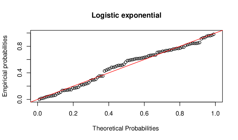
For the purpose of goodness-of-fit test, we consider different plots in Figures $3$, $4$, $5$ and $6$ to show that the LE distribution fits the real data set well. In Figure $3$, $Q$-$Q$ plots are used to compare the given data set to the theoretical model. Here, $Q$-$Q$ plot represents the points $(F^{-1}(i/(n+1);\hat{\alpha},\hat{\lambda}),x_{(i)})$, where $i=1,\ldots,n$, and $x_{(i)}$ represents the ordered values of given real data. In Figure $4$ , $P$-$P$ plot represents the points $(F(x_{i};\hat{\alpha},\hat{\lambda}),F_{n}(x_{(i)}))$, where $F_{n}(x_{(i)})=(1/n)\sum_{i=1}^{n}I(X\leq x_{(i)})$ is the empirical distribution function and I is the indicator function. In Figure $5$, empirical cumulative distribution function (ECDF) plots have been made which represent the CDFs of the corresponding distributions for observed data and it is compared with theoretical CDFs. In Figure $6$, plots of histogram of real data set and theoretical densities of associated distributions have been made. From all these it has been noticed that LE distributions fits the real data set better than the other above mentioned distributions.

In Table $10$, the MLEs and the Bayes estimates are obtained for the parameters of the LE distributions based on the real data set. In Table $11$, $90\%$ and $95\%$ approximate confidence and HPD credible intervals are tabulated. From Table $10$ , it is clear that the values of the estimates remain moderately close to each other. From Table $11$, it is clear that the length of the HPD credible intervals are smaller than that of the asymptotic confidence intervals. In a lifetime experiment, the choice of an optimal censoring scheme from a class of all possible censoring schemes has gained considerable attention in recent years. For example, one can see Pradhan and Kundu 2013 and Bhattacharya and Pradhan 2017. $A$-optimality and $D$-optimality criteria are mostly used criteria to choose an optimal censoring scheme for the distributions having more than one parameter. In the case of the $A$-optimality criterion, we have to minimize the trace, and for $D$-optimality, we have to minimize the determinant of the inverse of the observed Fisher information matrix. Comparison of different censoring schemes based on these two criteria is reported in Table $10$. Here, $A$-optimality is considered as C-I, and $D$-optimality is considered as C-II. Based on these two criterion, when $(n,m)$ is considered as $(100,20)$ then $(0*19,80*1)$ is optimal among other selected censoring schemes and when $(n,m)$ is considered as $(100,40)$ then $(0*39,60*1)$ is optimal among other selected censoring schemes, which have been reported in Table $10.$

Table 9: The MLEs and statistics for goodness-of-fit test.

	Model	$\widehat{\alpha}$	$\widehat{\lambda}$		-logL			AIC		AICC		BIC		K-S distance		p-value
	LED	3.0172	0.2750		143.2473			290.4946		290.6183		295.7049		0.0837		0.4601
	ED	——–	0.3185		196.3709			394.7418		394.7826		397.3469		0.2630		1.35 $\times 10^{-6}$
	IED	——–	2.1399		199.3956			400.7912		400.8320		403.3963		0.3577		5.83 $\times 10^{-12}$
	EED	7.7854	1.0131		146.1823			296.3646		296.4883		301.5749		0.1078		0.1819
	IWD	1.7689	3.0884		173.1440			350.2880		350.4117		355.4983		0.1777		0.0031
	GD	5.9529	2.2710		168.9527			341.9504		342.0291		347.1157		0.0935		0.3254

Table 10: Values of estimates of $\alpha$ and $\lambda$ for the real data set.

(n,m)	$T$	scheme	Prior	$\theta$	MLE		LLF			GELF		SELF	C-I	C-II
						$p=-0.05$	$p=0.5$	$p=1$	$q=-0.5$	$q=-0.25$	$q=0.25$
(100,20)	2	(0*19,80*1)	U	$\alpha$	2.8522	2.9576	2.9574	2.9573	2.9581	2.9579	2.9577	2.9576	0.3222	$1.24\times 10^{-4}$
				$\lambda$	0.2833	0.2725	0.2724	0.2722	0.2726	0.2725	0.2724	0.2725
			B	$\alpha$		2.9340	2.9338	2.9335	2.9339	2.9339	2.9338	2.9340
				$\lambda$		0.2875	0.2874	0.2873	0.2871	0.2869	0.2865	0.2875
		(0*10,8*10)	U	$\alpha$	3.5384	3.4594	3.4570	3.4549	3.4586	3.4583	3.4576	3.4592	0.4853	$1.58\times 10^{-4}$
				$\lambda$	0.3285	0.2840	0.2839	0.2838	0.2837	0.2836	0.2834	0.2840
			B	$\alpha$		3.4806	3.4798	3.4791	3.4803	3.4802	3.4800	3.4806
				$\lambda$		0.2927	0.2925	0.2923	0.2920	0.2917	0.2911	0.2926
		(80*1,0*19)	U	$\alpha$	4.6082	4.1443	4.1293	4.1159	4.1396	4.1380	4.1347	4.1429	0.6534	$6.59\times 10^{-4}$
				$\lambda$	0.5377	0.4868	0.4866	0.4863	0.2837	0.4863	0.4860	0.4855
			B	$\alpha$		4.4203	4.4161	4.4124	4.4191	4.4186	4.4177	4.4199
				$\lambda$		0.4767	0.4758	0.4749	0.4749	0.4740	0.4733	0.4766
(100,40)	2	(0*39,60*1)	U	$\alpha$	2.6357	2.7402	2.7391	2.7381	2.7398	2.7396	2.7392	2.7401	0.1845	$0.55\times 10^{-4}$
				$\lambda$	0.2699	0.2831	0.2829	0.2828	0.2826	0.2824	0.2820	0.2830
			B	$\alpha$		2.7146	2.7133	2.7121	2.7140	2.7138	2.7134	2.7144
				$\lambda$		0.2884	0.2883	0.2881	0.2883	0.2882	0.2880	0.2884
		(0*20,3*20)	U	$\alpha$	2.8287	2.8668	2.8653	2.8640	2.8661	2.8659	2.8655	2.8666	0.2113	$0.60\times 10^{-4}$
				$\lambda$	0.2831	0.2715	0.2714	0.2712	0.2713	0.2712	0.2711	0.2715
			B	$\alpha$		2.8372	2.8369	2.8366	2.8371	2.8370	2.8370	2.8372
				$\lambda$		0.2621	0.2620	0.2619	0.2618	0.2616	0.2613	0.2621
		(60*1,0*39)	U	$\alpha$	3.5248	3.4427	3.4406	3.4391	3.4416	3.4414	3.4409	3.4421	0.2795	$1.50\times 10^{-4}$
				$\lambda$	0.4144	0.3921	0.3919	0.3918	0.3917	0.3916	0.3913	0.3920
			B	$\alpha$		3.4522	3.4506	3.4490	3.4517	3.4515	3.4510	3.4521
				$\lambda$		0.4017	0.4016	0.4014	0.4014	0.4019	0.4010	0.4018

Table 11: Lengths of interval estimates of $\alpha$ and $\lambda$ for the real data set.

					90$\%$ confidence interval					95$\%$ confidence interval
(n,m)	T	scheme	$\theta$	NA	NL	HPD			NA	NL	HPD
(100,20)	2	(0*19,80*1)	$\alpha$	1.8704	1.9041	1.0766			2.2218	2.2784	1.1828
			$\lambda$	0.0994	0.0999	0.0896			0.1181	0.1189	0.0962
		(0*10,8*10)	$\alpha$	2.2972	2.3377	1.2671			2.7288	2.7969	1.2813
			$\lambda$	0.0901	0.0904	0.0783			0.1069	0.1075	0.0856
		(80*1,0*19)	$\alpha$	2.6654	2.7027	1.6717			3.1662	3.2288	1.7505
			$\lambda$	0.1058	0.1060	0.0970			0.1257	0.1260	0.1134
(100,40)	2	(0*39,60*1)	$\alpha$	1.4159	1.4330	0.7204			1.6819	1.7106	0.8520
			$\lambda$	0.0721	0.0724	0.0677			0.0857	0.0861	0.0798
		(0*20,3*20)	$\alpha$	1.5153	1.5335	0.7437			1.8000	1.8305	0.7642
			$\lambda$	0.0699	0.0702	0.0627			0.0831	0.0834	0.0792
		(60*1,0*39)	$\alpha$	1.7432	1.7611	0.8626			2.0707	2.1006	0.9248
			$\lambda$	0.0767	0.0769	0.0660			0.0911	0.0912	0.0865

Figure 3: Q-Q plots for various distributions fitted to the assumed real data set.

Figure 4: The P-P plots for various distributions fitted to the assumed real data set.

Figure 5: The ECDF vs. CDF plots for various distributions fitted to the assumed real data set.

Figure 6: The histogram and density plots for various distributions fitted to the assumed real data set.

8 Conclusion

In this article, statistical inference for the LE distribution under PT-IHCS has been discussed. The MLEs are obtained. The forms of the MLEs can not be expressed explicitly. Thus, Newton-Raphson iterative method is employed to compute the MLEs of the parameters. In Bayesian study, independent and bivariate priors are considered. Three loss functions are utilized. The Bayes estimates are difficult to get in closed forms. They are of the form of the ratio of two integrals. To evaluate approximate Bayes estimates, Lindley’s approximation technique is applied. The HPD credible intervals are obtained by using importance sampling method. In addition to the HPD credible intervals, two methods are employed to computed the asymptotic confidence intervals of the model parameters. Monte Carlo simulation study is performed to compare the performance of the proposed estimates. From the numerical study, it is observed that the Bayes estimates with respect to the independent prior distributions perform better than the other estimates in terms of the average values and the MSEs. Further, a real dataset is considered for illustrative purposes.


Acknowledgement: The authors would like to thank the Editor in Chief, an Associate Editor and anonymous reviewers for their positive remarks and useful comments. The author S. Dutta, thanks the Council of Scientific and Industrial Research (C.S.I.R. Grant No. 09/983(0038)/2019-EMR-I), India, for the financial assistantship received to carry out this research work. Both the authors thanks the research facilities received from the Department of Mathematics, National Institute of Technology Rourkela, India.

Disclosure Statement: Both the authors declare that they do not have any conflict of interest.

Appendix A Appendix

In Subsection $3.1$, Bayes estimates based on univariate prior are obtained and the posterior density function has a term $k_{1}$ which is expressed as

$$k_{1} = \int_{0}^{\infty}\int_{0}^{\infty}\alpha^{D+a-1}\lambda^{D+c-1}e^{-b\alpha}e^{-\lambda(d-\sum_{i=1}^{D}x_{i})}\prod_{i=1}^{D}(g(x_{i};\lambda))^{\alpha-1}[1+(g(x_{i};\lambda))^{\alpha}]^{-(R_{i}+2)}$$ (A.1)

$$\times[1+(g(T;\lambda))^{\alpha}]^{-R^{*}_{D}}d\alpha d\lambda.$$

Similarly, to obtain Bayes estimates based on bivariate prior the posterior density function has a term $k_{2}$ which is expressed as

$$k_{2} = \int_{0}^{\infty}\int_{0}^{\infty}\alpha^{D}\lambda^{D+c-2}e^{-\lambda(d-\sum_{i=1}^{D}x_{i})}\prod_{i=1}^{D}(g(x_{i};\lambda))^{\alpha-1}[1+(g(x_{i};\lambda))^{\alpha}]^{-(R_{i}+2)}$$ (A.2)

$$\times[1+(g(T;\lambda))^{\alpha}]^{-R^{*}_{D}}d\alpha~d\lambda.$$

In Subsection $4.2$, the posterior density has a weight function of $\alpha$ and $\lambda$ which is expressed as

$$h(\alpha,\lambda) = \left[b-\sum_{i=1}^{D}\log(g(x_{i};\lambda))\right]^{-(D+a)}\left(d-\sum_{i=1}^{D}x_{i}\right)^{-(D+c)}\left[1+(g(T;\lambda))^{\alpha}\right]^{-R^{*}_{D}}$$ (A.3)

$$\times\prod_{i=1}^{D}\frac{\left[1+(g(x_{i};\lambda))^{\alpha}\right]^{-(R_{i}+2)}}{g(x_{i};\lambda)}.$$

.

Appendix B Appendix

In this part of the paper, the Lindley’s approximation method is described. However, one may refer to Lindley 1980 for further elaboration. Consider an arbitrary function of $\alpha$ and $\lambda$, say $\phi(\alpha,\lambda)$. The forms of the Bayes estimators (see Eqs. (3.4), (3.5) and (3.6)) involve expectations with respect to the posterior probability density function. The posterior mean of $\phi(\alpha,\lambda)$ is given by

$$E(\phi(\alpha,\lambda)|\underline{x})=\frac{\int_{0}^{\infty}\int_{0}^{\infty}\phi(\alpha,\lambda)e^{l(\alpha,\lambda|\underline{x})+P(\alpha,\lambda)}d\alpha d\lambda}{\int_{0}^{\infty}\int_{0}^{\infty}e^{l(\alpha,\lambda|\underline{x})+P(\alpha,\lambda)}d\alpha d\lambda},$$ (B.1)

where $l(\alpha,\lambda|\underline{x})$ is the log-likelihood function and $P(\alpha,\lambda)$ is the logarithm of joint prior distribution of $\alpha$ and $\lambda$. Using the method due to Lindley 1980, (B.1) can be approximated as

$$E(\phi(\alpha,\lambda)|\underline{x})\approx\phi(\alpha,\lambda)+\frac{1}{2}\left(A+l_{30}B_{12}+l_{03}B_{21}+l_{21}C_{12}+l_{12}C_{21}+2P_{1}A_{12}+2P_{2}A_{21}\right),$$

where $A=\sum_{i=1}^{2}\sum_{j=1}^{2}v_{ij}\tau_{ij}$ , $\theta_{1}=\alpha$, $\theta_{2}=\lambda,$ $v_{i}=\frac{\partial\phi}{\partial\theta_{i}}$ , $v_{ij}=\frac{\partial^{2}\phi}{\partial\theta_{i}\partial\theta_{j}}$, $P_{i}=\frac{\partial P}{\partial\theta_{i}}$ , $A_{ij}=v_{i}\tau_{ii}+v_{j}\tau_{ji}$ , $B_{ij}=(v_{i}\tau_{ii}+v_{j}\tau_{ij})\tau_{ii}$ , $C_{ij}=3v_{i}\tau_{ii}\tau_{ij}+v_{j}(\tau_{ii}\tau_{jj}+2\tau^{2}_{ij})$ , $l_{ij}=\frac{\partial^{i+j}l}{\partial\theta^{i}_{1}\theta^{j}_{2}}$ , $P=\log\pi_{3}(\theta_{1},\theta_{2})$ and $\tau_{ij}$ is the $(i,j)$th element of $\left[-\frac{\partial^{2}l}{\partial\theta^{i}_{1}\partial\theta^{j}_{2}}\right]^{-1}$, where $i,~j=1,~2$. For the present problem, the loglikelihood function can be written as

$$l = D\log\alpha+D\log\lambda+\lambda\sum_{i=1}^{D}x_{i}+(\alpha-1)\sum_{i=1}^{D}\log(g(x_{i};\lambda))-\sum_{i=1}^{D}(R_{i}+2)\log U$$ (B.3)

$$-R^{*}_{D}\log V,$$

where $U\equiv U(\alpha,\lambda)=1+(g(x_{i};\lambda))^{\alpha}$ and $V\equiv V(\alpha,\lambda)=1+(g(T;\lambda))^{\alpha}$. Next, the required partial derivatives of $l$ with respect to $\alpha$ and $\lambda$ are presented.

$$l_{10} = \frac{\partial l}{\partial\alpha}=\frac{D}{\alpha}+\sum_{i=1}^{D}\log(g(x_{i};\lambda))-\sum_{i=1}^{D}(R_{i}+2)\frac{U_{\alpha}}{U}-R^{*}_{D}\frac{V_{\alpha}}{V}$$

$$l_{01} = \frac{\partial l}{\partial\lambda}=\frac{D}{\lambda}+\sum_{i=1}^{D}x_{i}+(\alpha-1)\sum_{i=1}^{D}\frac{x_{i}e^{\lambda x_{i}}}{g(x_{i};\lambda)}-\sum_{i=1}^{D}(R_{i}+2)\frac{U_{\lambda}}{U}-R^{*}_{D}\frac{V_{\lambda}}{V}$$

$$l_{20} = \frac{\partial^{2}l}{\partial\alpha^{2}}=-\frac{D}{\alpha^{2}}-\sum_{i=1}^{D}(R_{i}+2)\left[\frac{UU_{\alpha\alpha}-U^{2}_{\alpha}}{U^{2}}\right]-R^{*}_{D}\left[\frac{VV_{\alpha\alpha}-V^{2}_{\alpha}}{V^{2}}\right]$$

$$l_{02} = \frac{\partial^{2}l}{\partial\lambda^{2}}=-\frac{D}{\lambda^{2}}-(\alpha-1)\sum_{i=1}^{D}\frac{x^{2}_{i}e^{\lambda x_{i}}}{(g(x_{i};\lambda))^{2}}-\sum_{i=1}^{D}(R_{i}+2)\left[\frac{UU_{\lambda\lambda}-U^{2}_{\lambda}}{U^{2}}\right]$$

$$-R^{*}_{D}\left[\frac{VV_{\lambda\lambda}-V^{2}_{\lambda}}{V^{2}}\right]$$

$$l_{11} = \frac{\partial^{2}l}{\partial\alpha\partial\lambda}=\sum_{i=1}^{D}\frac{x_{i}e^{\lambda x_{i}}}{g(x_{i};\lambda)}-\sum_{i=1}^{D}(R_{i}+2)\left[\frac{UU_{\alpha\lambda}-U_{\alpha}U_{\lambda}}{U^{2}}\right]-R^{*}_{D}\left[\frac{VV_{\alpha\lambda}-V_{\alpha}V_{\lambda}}{V^{2}}\right]$$

$$l_{30} = \frac{\partial^{3}l}{\partial\alpha^{3}}=\frac{2D}{\alpha^{3}}-\sum_{i=1}^{D}(R_{i}+2)\left[\frac{U^{2}U_{\alpha\alpha\alpha}-3UU_{\alpha}U_{\alpha\alpha}+2U^{3}_{\alpha}}{U^{3}}\right]$$

$$-R^{*}_{D}\left[\frac{V^{2}V_{\alpha\alpha\alpha}-3VV_{\alpha}V_{\alpha\alpha}+2V^{3}_{\alpha}}{V^{3}}\right]$$

$$l_{03} = \frac{\partial^{3}l}{\partial\lambda^{3}}=(\alpha-1)\sum_{i=1}^{D}x^{3}_{i}\left[\frac{e^{\lambda x_{i}}(1+e^{\lambda x_{i}})}{(g(x_{i};\lambda))^{3}}\right]-\sum_{i=1}^{D}(R_{i}+2)\left[\frac{U^{2}U_{\lambda\lambda\lambda}-3UU_{\lambda}U_{\lambda\lambda}+2U^{3}_{\lambda}}{U^{3}}\right]$$

$$-R^{*}_{D}\left[\frac{V^{2}V_{\lambda\lambda\lambda}-3VV_{\lambda}V_{\lambda\lambda}+2V^{3}_{\lambda}}{V^{3}}\right]+\frac{2D}{\lambda^{3}}$$

$$l_{21} = \frac{\partial^{3}l}{\partial\alpha^{2}\partial\lambda}=-\sum_{i=1}^{D}(R_{i}+2)\left[\frac{U(UU_{\alpha\alpha\lambda}-U_{\lambda}U_{\alpha\alpha}-2U_{\alpha}U_{\alpha\lambda})+2U^{2}_{\alpha}U_{\lambda}}{U^{3}}\right]$$

$$-R^{*}_{D}\left[\frac{V(VV_{\alpha\alpha\lambda}-V_{\lambda}V_{\alpha\alpha}-2V_{\alpha}V_{\alpha\lambda})+2V^{2}_{\alpha}V_{\lambda}}{V^{3}}\right]$$

$$l_{12} = \frac{\partial^{3}l}{\partial\alpha\partial\lambda^{2}}=-\sum_{i=1}^{D}(R_{i}+2)\left[\frac{U(UU_{\alpha\lambda\lambda}-U_{\alpha}U_{\lambda\lambda}-2U_{\lambda}U_{\alpha\lambda})+2U_{\alpha}U^{2}_{\lambda}}{U^{3}}\right]$$

$$-R^{*}_{D}\left[\frac{V(VV_{\alpha\lambda\lambda}-V_{\alpha}V_{\lambda\lambda}-2V_{\lambda}V_{\alpha\lambda})+2V_{\alpha}V^{2}_{\lambda}}{V^{3}}\right]-\sum_{i=1}^{D}x^{2}_{i}\left[\frac{e^{\lambda x_{i}}}{(g(x_{i};\lambda))^{2}}\right]$$

where

$$U_{\alpha} = (e^{\lambda x_{i}}-1)^{\alpha}\log(g(x_{i};\lambda))$$

$$V_{\alpha} = (g(T;\lambda))^{\alpha}\log(g(T;\lambda))$$

$$U_{\lambda} = \alpha x_{i}e^{\lambda x_{i}}(g(x_{i};\lambda))^{\alpha-1}$$

$$V_{\lambda} = \alpha Te^{\lambda T}(g(T;\lambda))^{\alpha-1}$$

$$U_{\alpha\lambda} = x_{i}e^{\lambda x_{i}}(g(x_{i};\lambda))^{\alpha-1}\left[\alpha\log(g(x_{i};\lambda))+1\right]$$

$$V_{\alpha\lambda} = Te^{\lambda T}(g(T;\lambda))^{\alpha-1}\left[\alpha\log(g(T;\lambda))+1\right]$$

$$U_{\alpha\alpha} = (g(x_{i};\lambda))^{\alpha}\left[\log(g(x_{i};\lambda))\right]^{2}$$

$$V_{\alpha\alpha} = (g(T;\lambda))^{\alpha}\left[\log(g(T;\lambda))\right]^{2}$$

$$U_{\lambda\lambda} = \alpha x^{2}_{i}e^{\lambda x_{i}}(g(x_{i};\lambda))^{\alpha-2}(\alpha e^{\lambda x_{i}}-1)$$

$$V_{\lambda\lambda} = \alpha T^{2}e^{\lambda T}(g(T;\lambda))^{\alpha-2}(\alpha e^{\lambda T}-1)$$

$$U_{\alpha\alpha\alpha} = (g(x_{i};\lambda))^{\alpha}\left[\log(g(x_{i};\lambda))\right]^{3}$$

$$V_{\alpha\alpha\alpha} = (g(T;\lambda))^{\alpha}\left[\log(g(T;\lambda))\right]^{3}$$

$$U_{\lambda\lambda\lambda} = \alpha x^{3}_{i}e^{\lambda x_{i}}(g(x_{i};\lambda))^{\alpha-3}\left[\alpha^{2}e^{2\lambda x_{i}}+(1-3\alpha)e^{\lambda x_{i}}+1\right]$$

$$V_{\lambda\lambda\lambda} = \alpha T^{3}e^{\lambda T}(g(T;\lambda))^{\alpha-3}\left[\alpha^{2}e^{2\lambda T}+(1-3\alpha)e^{\lambda T}+1\right]$$

$$U_{\alpha\alpha\lambda} = x_{i}e^{\lambda x_{i}}(g(x_{i};\lambda))^{\alpha-1}\log(g(x_{i};\lambda))\left[\alpha\log(g(x_{i};\lambda))+2\right]$$

$$V_{\alpha\alpha\lambda} = Te^{\lambda T}(g(T;\lambda))^{\alpha-1}\log(g(T;\lambda))\left[\alpha\log(g(T;\lambda))+2\right]$$

$$U_{\alpha\lambda\lambda} = x^{2}_{i}e^{\lambda x_{i}}(g(x_{i};\lambda))^{\alpha-2}\left[\alpha(\alpha e^{\lambda x_{i}}-1)\log(g(x_{i};\lambda))+2\alpha e^{\lambda x_{i}}-1\right]$$

$$V_{\alpha\lambda\lambda} = T^{2}e^{\lambda T}(g(T;\lambda))^{\alpha-2}\left[\alpha(\alpha e^{\lambda T}-1)\log(g(T;\lambda))+2\alpha e^{\lambda T}-1\right].$$

References

- (1)
- Arnold and Press (1983) Arnold, B. C. and Press, S. J. (1983). Bayesian inference for Pareto populations, Journal of Econometrics. 21(3), 287–306.
- Bhattacharya and Pradhan (2017) Bhattacharya, R. and Pradhan, B. (2017). Computation of optimum type-ii progressively hybrid censoring schemes using variable neighborhood search algorithm, Test. 26(4), 802–821.
- Calabria and Pulcini (1994) Calabria, R. and Pulcini, G. (1994). Bayes 2-sample prediction for the inverse Weibull distribution, Communications in Statistics-Theory and Methods. 23(6), 1811–1824.
- Chen and Shao (1999) Chen, M. H. and Shao, Q. M. (1999). Monte Carlo estimation of Bayesian credible and HPD intervals, Journal of Computational and Graphical Statistics. 8(1), 69–92.
- Epstein (1954) Epstein, B. (1954). Truncated life tests in the exponential case, The Annals of Mathematical Statistics. 25(3), 555–564.
- Gamchi et al. (2019) Gamchi, F. V., Alma, Ö. G. and Belaghi, R. A. (2019). Classical and Bayesian inference for Burr type-III distribution based on progressive type-II hybrid censored data, Mathematical Sciences. 13(2), 79–95.
- Goyal et al. (2020) Goyal, T., Rai, P. K. and Maurya, S. K. (2020). Bayesian estimation for GDUS exponential distribution under type-I progressive hybrid censoring, Annals of Data Science. 7(2), 307–345.
- Hemmati and Khorram (2013) Hemmati, F. and Khorram, E. (2013). Statistical analysis of the log-normal distribution under type-II progressive hybrid censoring schemes, Communications in Statistics-simulation and Computation. 42(1), 52–75.
- Hjorth (1980) Hjorth, U. (1980). A reliability distribution with increasing, decreasing, constant and bathtub-shaped failure rates, Technometrics. 22(1), 99–107.
- Kayal et al. (2019) Kayal, T., Tripathi, Y. M., Kundu, D. and Rastogi, M. (2019). Statistical inference of Chen distribution based on type-I progressive hybrid censored samples, Statistics, Optimization & Information Computing. .
- Kundu and Joarder (2006) Kundu, D. and Joarder, A. (2006). Analysis of Type-II progressively hybrid censored data, Computational Statistics & Data Analysis. 50(10), 2509–2528.
- Kuş (2007) Kuş, C. (2007). A new lifetime distribution, Computational Statistics & Data Analysis. 51(9), 4497–4509.
- Lan and Leemis (2008) Lan, Y. and Leemis, L. M. (2008). The logistic–exponential survival distribution, Naval Research Logistics. 55(3), 252–264.
- Lin et al. (2009) Lin, C.-T., Ng, H. K. T. and Chan, P. S. (2009). Statistical inference of type-II progressively hybrid censored data with Weibull lifetimes, Communications in Statistics – Theory and Methods. 38(10), 1710–1729.
- Lindley (1980) Lindley, D. V. (1980). Approximate Bayesian methods, Trabajos de estadística y de investigación operativa. 31(1), 223–245.
- Mäkeläinen et al. (1981) Mäkeläinen, T., Schmidt, K. and Styan, G. P. (1981). On the existence and uniqueness of the maximum likelihood estimate of a vector-valued parameter in fixed-size samples, The Annals of Statistics. 9(4), 758–767.
- Meeker and Escobar (2014) Meeker, W. Q. and Escobar, L. A. (2014). Statistical methods for reliability data, John Wiley & Sons.
- Nichols and Padgett (2006) Nichols, M. D. and Padgett, W. (2006). A bootstrap control chart for weibull percentiles, Quality and reliability engineering international. 22(2), 141–151.
- Pradhan and Kundu (2013) Pradhan, B. and Kundu, D. (2013). Inference and optimal censoring schemes for progressively censored Birnbaum–Saunders distribution, Journal of Statistical Planning and Inference. 143(6), 1098–1108.
- Sultana et al. (2019) Sultana, F., Tripathi, Y. and Kumar Rastogi, M. (2019). Parameter estimation and prediction for the generalized half normal distribution under progressive hybrid censoring, Journal of The Iranian Statistical Society. 18(1), 191–236.
- Sultana et al. (2020) Sultana, F., Tripathi, Y. M., Wu, S. J. and Sen, T. (2020). Inference for Kumaraswamy distribution based on type-I progressive hybrid censoring, Annals of Data Science. pp. 1–25.
- Varian (1975) Varian, H. R. (1975). A Bayesian approach to real estate assessment, In Studies in Bayesian econometrics and statistics in honor of Leonard J. Savage, eds Fienberg Stephen E., and A. Zellner. pp. 195–208.