Logic Tensor Networks

Abstract

Attempts at combining logic and neural networks into neurosymbolic approaches have been on the increase in recent years. In a neurosymbolic system, symbolic knowledge assists deep learning, which typically uses a sub-symbolic distributed representation, to learn and reason at a higher level of abstraction. We present Logic Tensor Networks (LTN), a neurosymbolic framework that supports querying, learning and reasoning with both rich data and abstract knowledge about the world. LTN introduces a fully differentiable logical language, called Real Logic, whereby the elements of a first-order logic signature are grounded onto data using neural computational graphs and first-order fuzzy logic semantics. We show that LTN provides a uniform language to represent and compute efficiently many of the most important AI tasks such as multi-label classification, relational learning, data clustering, semi-supervised learning, regression, embedding learning and query answering. We implement and illustrate each of the above tasks with several simple explanatory examples using TensorFlow 2. The results indicate that LTN can be a general and powerful framework for neurosymbolic AI.

1 Introduction

Artificial Intelligence (AI) agents are required to learn from their surroundings and reason about what has been learned to make decisions, act in the world, or react to various stimuli. The latest Machine Learning (ML) has adopted mostly a pure sub-symbolic learning approach. Using distributed representations of entities, the latest ML performs quick decision-making without building a comprehensible model of the world. While achieving impressive results in computer vision, natural language, game playing, and multimodal learning, such approaches are known to be data inefficient and to struggle at out-of-distribution generalization. Although the use of appropriate inductive biases can alleviate such shortcomings, in general, sub-symbolic models lack comprehensibility. By contrast, symbolic AI is based on rich, high-level representations of the world that use human-readable symbols. By rich knowledge, we refer to logical representations which are more expressive than propositional logic or propositional probabilistic approaches, and which can express knowledge using full first-order logic, including universal and existential quantification ($\forall x$ and $\exists y$), arbitrary $n$-ary relations over variables, e.g. $R(x,y,z,\dots)$, and function symbols, e.g. $\mathrm{fatherOf}(x)$, $x+y$, etc. Symbolic AI has achieved success at theorem proving, logical inference, and verification. However, it also has shortcomings when dealing with incomplete knowledge. It can be inefficient with large amounts of inaccurate data and lack robustness to outliers. Purely symbolic decision algorithms usually have high computational complexity making them impractical for the real world. It is now clear that the predominant approach to ML, where learning is based on recognizing the latent structures hidden in the data, is insufficient and may benefit from symbolic AI [17]. In this context, neurosymbolic AI, which stems from neural networks and symbolic AI, attempts to combine the strength of both paradigms (see [16, 40, 54] for recent surveys). That is to say, combine reasoning with complex representations of knowledge (knowledge-bases, semantic networks, ontologies, trees, and graphs) with learning from complex data (images, time series, sensorimotor data, natural language). Consequently, a main challenge for neurosymbolic AI is the grounding of symbols, including constants, functional and relational symbols, into real data, which is akin to the longstanding symbol grounding problem [30].

Logic Tensor Networks (LTN) are a neurosymbolic framework and computational model that supports learning and reasoning about data with rich knowledge. In LTN, one can represent and effectively compute the most important tasks of deep learning with a fully differentiable first-order logic language, called Real Logic, which adopts infinitely many truth-values in the interval [0,1] [22, 25]. In particular, LTN supports the specification and computation of the following AI tasks uniformly using the same language: data clustering, classification, relational learning, query answering, semi-supervised learning, regression, and embedding learning.

LTN and Real Logic were first introduced in [62]. Since then, LTN has been applied to different AI tasks involving perception, learning, and reasoning about relational knowledge. In [18, 19], LTN was applied to semantic image interpretation whereby relational knowledge about objects was injected into deep networks for object relationship detection. In [6], LTN was evaluated on its capacity to perform reasoning about ontological knowledge. Furthermore, [7] shows how LTN can be used to learn an embedding of concepts into a latent real space by taking into consideration ontological knowledge about such concepts. In [3], LTN is used to annotate a reinforcement learning environment with prior knowledge and incorporate latent information into an agent. In [42], authors embed LTN in a state-of-the-art convolutional object detector. Extensions and generalizations of LTN have also been proposed in the past years, such as LYRICS [47] and Differentiable Fuzzy Logic (DFL) [68, 69]. LYRICS provides an input language allowing one to define background knowledge using a first-order logic where predicate and function symbols are grounded onto any computational graph. DFL analyzes how a large collection of fuzzy logic operators behave in a differentiable learning setting. DFL also introduces new semantics for fuzzy logic implications called sigmoidal implications, and it shows that such semantics outperform other semantics in several semi-supervised machine learning tasks.

This paper provides a thorough description of the full formalism and several extensions of LTN. We show using an extensive set of explanatory examples, how LTN can be applied to solve many ML tasks with the help of logical knowledge. In particular, the earlier versions of LTN have been extended with: (1) Explicit domain declaration: constants, variables, functions and predicates are now domain typed (e.g. the constants John and Paris can be from the domain of person and city, respectively). The definition of structured domains is also possible (e.g. the domain couple can be defined as the Cartesian product of two domains of persons); (2) Guarded quantifiers: guarded universal and existential quantifiers now allow the user to limit the quantification to the elements that satisfy some Boolean condition, e.g. $\forall x:\mathrm{age}(x)<10\>(\mathrm{playsPiano}(x)\rightarrow\mathrm{enfantProdige}(x))$ restricts the quantification to the cases where $age$ is lower than 10; (3) Diagonal quantification: Diagonal quantification allows the user to write statements about specific tuples extracted in order from $n$ variables. For example, if the variables $\mathrm{capital}$ and $\mathrm{country}$ both have $k$ instances such that the $i$-th instance of $\mathrm{capital}$ corresponds to the $i$-th instance of $\mathrm{country}$, one can write $\forall\mathrm{Diag}(\mathrm{capital},\mathrm{country})\>\mathrm{capitalOf}(\mathrm{capital},\mathrm{country})$.

Inspired by the work of [69], this paper also extends the product t-norm configuration of LTN with the generalized mean aggregator, and it introduces solutions to the vanishing or exploding gradient problems. Finally, the paper formally defines a semantic approach to refutation-based reasoning in Real Logic to verify if a statement is a logical consequence of a knowledge base. Example 4.8 proves that this new approach can better capture logical consequences compared to simply querying unknown formulas after learning (as done in [6]).

The new version of LTN has been implemented in TensorFlow 2 [1]. Both the LTN library and the code for the examples used in this paper are available at https://github.com/logictensornetworks/logictensornetworks.

The remainder of the paper is organized as follows: In Section 2, we define and illustrate Real Logic as a fully-differentiable first-order logic. In Section 3, we specify learning and reasoning in Real Logic and its modeling into deep networks with Logic Tensor Networks (LTN). In Section 4, we illustrate the reach of LTN by investigating a range of learning problems from clustering to embedding learning. In Section 5, we place LTN in the context of the latest related work in neurosymbolic AI. In Section 6 we conclude and discuss directions for future work. The Appendix contains information about the implementation of LTN in TensorFlow 2, experimental set-ups, the different options for the differentiable logic operators, and a study of their relationship with gradient computations.

2 Real Logic

2.1 Syntax

Real Logic forms the basis of Logic Tensor Networks. Real Logic is defined on a first-order language $\mathcal{L}$ with a signature that contains a set $\mathcal{C}$ of constant symbols (objects), a set $\mathcal{F}$ of functional symbols, a set $\mathcal{P}$ of relational symbols (predicates), and a set $\mathcal{X}$ of variable symbols. $\mathcal{L}$-formulas allow us to specify relational knowledge with variables, e.g. the atomic formula $\mathrm{is\_friend}(v_{1},v_{2})$ may state that the person $v_{1}$ is a friend of the person $v_{2}$, the formula $\forall x\forall y(\mathrm{is\_friend}(x,y)\rightarrow\mathrm{is\_friend}(y,x))$ states that the relation $\mathrm{is\_friend}$ is symmetric, and the formula $\forall x(\exists y(\mathrm{Italian}(x)\land\mathrm{is\_friend}(x,y)))$ states that every person has a friend that is Italian. Since we are interested in learning and reasoning in real-world scenarios where degrees of truth are often fuzzy and exceptions are present, formulas can be partially true, and therefore we adopt fuzzy semantics.

Objects can be of different types. Similarly, functions and predicates are typed. Therefore, we assume there exists a non-empty set of symbols $\mathcal{D}$ called domain symbols. To assign types to the elements of $\mathcal{L}$ we introduce the functions $\mathbf{D}$, $\mathbf{D_{in}}$ and $\mathbf{D_{out}}$ such that:

• $\mathbf{D}:\mathcal{X}\cup\mathcal{C}\rightarrow\mathcal{D}$. Intuitively, $\mathbf{D}(x)$ and $\mathbf{D}(c)$ returns the domain of a variable $x$ or a constant $c$.

• $\mathbf{D_{in}}:\mathcal{F}\cup\mathcal{P}\rightarrow\mathcal{D}^{*}$, where $\mathcal{D}^{*}$ is the Kleene star of $\mathcal{D}$, that is the set of all finite sequences of symbols in $\mathcal{D}$. Intuitively, $\mathbf{D_{in}}(f)$ and $\mathbf{D_{in}}(p)$ returns the domains of the arguments of a function $f$ or a predicate $p$. If $f$ takes two arguments (for example, $f(x,y)$), $\mathbf{D_{in}}(f)$ returns two domains, one per argument.

• $\mathbf{D_{out}}:\mathcal{F}\rightarrow\mathcal{D}$. Intuitively, $\mathbf{D_{out}}(f)$ returns the range of a function symbol.

Real Logic may also contain propositional variables, as follows: if $P$ is a 0-ary predicate with $\mathbf{D_{in}}(P)=\left<\>\right>$ (the empty sequence of domains) then $P$ is a propositional variable (an atom with truth-value in the interval [0,1]).

A term is constructed recursively in the usual way from constant symbols, variables, and function symbols. An expression formed by applying a predicate symbol to an appropriate number of terms with appropriate domains is called an atomic formula, which evaluates to $\mathit{true}$ or $\mathit{false}$ in classical logic and a number in $[0,1]$ in the case of Real Logic. We define the set of terms of the language as follows:

• each element $t$ of $\mathcal{X}\cup\mathcal{C}$ is a term of the domain $\mathbf{D}(t)$;

• if $t_{i}$ is a term of domain $\mathbf{D}(t_{i})$ for $1\leq i\leq n$ then $t_{1}t_{2}\dots t_{n}$ (the sequence composed of $t_{1}$ followed by $t_{2}$ and so on, up to $t_{n}$) is a term of the domain $\mathbf{D}(t_{1})\mathbf{D}(t_{2})\dots\mathbf{D}(t_{n})$;

• if $t$ is a term of the domain $\mathbf{D_{in}}(f)$ then $f(t)$ is a term of the domain $\mathbf{D_{out}}(f)$.

We allow the following set of formula in $\mathcal{L}$:

• $t_{1}=t_{2}$ is an atomic formula for any terms $t_{1}$ and $t_{2}$ with $\mathbf{D}(t_{1})=\mathbf{D}(t_{2})$;

• $p(t)$ is an atomic formula if $\mathbf{D}(t)=\mathbf{D_{in}}(p)$;

• If $\phi$ and $\psi$ are formula and $x_{1},\dots,x_{n}$ are $n$ distinct variable symbols then $\diamond\phi$, $\phi\circ\psi$ and $Qx_{1}\dots x_{n}\phi$ are formula, where $\diamond$ is a unary connective, $\circ$ is a binary connective and $Q$ is a quantifier.

We use $\diamond\in\{\lnot\}$ (negation), $\circ\in\{\land,\lor,\rightarrow,\leftrightarrow\}$ (conjunction, disjunction, implication and bi-conditional, respectively) and $Q\in\{\forall,\exists\}$ (universal and existential, respectively).

Example 1.

Let $\mathrm{Town}$ denote the domain of towns in the world and $\mathrm{People}$ denote the domain of living people. Suppose that $\mathcal{L}$ contains the constant symbols $\mathrm{Alice}$, $\mathrm{Bob}$ and $\mathrm{Charlie}$ of domain $\mathrm{People}$, and $\mathrm{Rome}$ and $\mathrm{Seoul}$ of domain $\mathrm{Town}$. Let $x$ be a variable of domain $\mathrm{People}$ and $u$ be a variable of domain $\mathrm{Town}$. The term $x,u$ (i.e. the sequence $x$ followed by $u$) has domain $\mathrm{People},\mathrm{Town}$ which denotes the Cartesian product between $\mathrm{People}$ and $\mathrm{Town}$ ($\mathrm{People}$ $\bigtimes$ $\mathrm{Town}$). $\mathrm{Alice},\mathrm{Rome}$ is interpreted as an element of the domain $\mathrm{People},\mathrm{Town}$. Let $\mathrm{lives\_in}$ be a predicate with input domain $\mathbf{D_{in}}(\mathrm{lives\_in})=\mathrm{People},\mathrm{Town}$. $\mathrm{lives\_in}(\mathrm{Alice},\mathrm{Rome})$ is a well-formed expression, whereas $\mathrm{lives\_in}(\mathrm{Bob},\mathrm{Charlie})$ is not.

2.2 Semantics of Real Logic

The semantics of Real Logic departs from the standard abstract semantics of First-order Logic (FOL). In Real Logic, domains are interpreted concretely by tensors in the real field. Every object denoted by constants, variables, and terms, is interpreted as a tensor of real values. Functions are interpreted as real functions or tensor operations. Predicates are interpreted as functions or tensor operations projecting onto a value in the interval $[0,1]$.

To emphasize the fact that in Real Logic symbols are grounded onto real-valued features, we use the term grounding, denoted by $\mathcal{G}$, in place of interpretation. Notice that this is different from the common use of the term grounding in logic, which indicates the operation of replacing the variables of a term or formula with constants or terms containing no variables. To avoid confusion, we use the synonym instantiation for this purpose. $\mathcal{G}$ associates a tensor of real numbers to any term of $\mathcal{L}$, and a real number in the interval $[0,1]$ to any formula $\phi$ of $\mathcal{L}$. Intuitively, $\mathcal{G}(t)$ are the numeric features of the objects denoted by $t$, and $\mathcal{G}(\phi)$ represents the system’s degree of confidence in the truth of $\phi$; the higher the value, the higher the confidence.

2.2.1 Grounding domains and the signature

A grounding for a logical language $\mathcal{L}$ on the set of domains $\mathcal{D}$ provides the interpretation of both the domain symbols in $\mathcal{D}$ and the non-logical symbols in $\mathcal{L}$.

Definition 1.

A grounding $\mathcal{G}$ associates to each domain $D\in\mathcal{D}$ a set $\mathcal{G}(D)\subseteq\bigcup\limits_{n_{1}\dots n_{d}\in\mathbb{N}^{*}}\mathbb{R}^{n_{1}\times\dots\times n_{d}}$. For every $D_{1}\dots D_{n}\in\mathcal{D}^{*}$, $\mathcal{G}(D_{1}\dots D_{n})=\bigtimes_{i=1}^{n}\mathcal{G}(D_{i})$, that is $\mathcal{G}(D_{1})\bigtimes\mathcal{G}(D_{2})\bigtimes...\bigtimes\mathcal{G}(D_{n})$.

Notice that the elements in $\mathcal{G}(D)$ may be tensors of any rank $d$ and any dimensions $n_{1}\times\dots\times n_{d}$, as $\mathbb{N}^{*}$ denotes the Kleene star of $\mathbb{N}$.

Example 2.

Let $\mathrm{digit\_images}$ denote a domain of images of handwritten digits. If we use images of $256\times 256$ RGB pixels, then $\mathcal{G}(\mathrm{digit\_images})\subseteq\mathbb{R}^{256\times 256\times 3}$. Let us consider the predicate $\mathrm{is\_digit}(\includegraphics[width=10.22217pt]{figures/mnist_eight.png},8)$. The terms $\includegraphics[width=10.22217pt]{figures/mnist_eight.png},8$ have domains $\mathrm{digit\_images},\mathrm{digits}$. Any input to the predicate is a tuple in $\mathcal{G}(\mathrm{digit\_images},\mathrm{digits})=\mathcal{G}(\mathrm{digit\_images})\times\mathcal{G}(\mathrm{digits})$.

A grounding assigns to each constant symbol $c$, a tensor $\mathcal{G}(c)$ in the domain $\mathcal{G}(\mathbf{D}(c))$; It assigns to a variable $x$ a finite sequence of tensors $d_{1}\dots d_{k}$, each in $\mathcal{G}(\mathbf{D}(x))$. These tensors represent the instances of $x$. Differently from in FOL where a variable is assigned to a single value of the domain of interpretations at a time, in Real Logic a variable is assigned to a sequence of values in its domain, the $k$ examples of $x$. A grounding assigns to a function symbol $f$ a function taking tensors from $\mathcal{G}(\mathbf{D_{in}}(f))$ as input, and producing a tensor in $\mathcal{G}(\mathbf{D_{out}}(f))$ as output. Finally, a grounding assigns to a predicate symbol $p$ a function taking tensors from $\mathcal{G}(\mathbf{D_{in}}(p))$ as input, and producing a truth-value in the interval $[0,1]$ as output.

Definition 2.

A grounding $\mathcal{G}$ of $\mathcal{L}$ is a function defined on the signature of $\mathcal{L}$ that satisfies the following conditions:

1. $\mathcal{G}(x)=\left<d_{1}\dots d_{k}\right>\in\bigtimes_{i=1}^{k}\mathcal{G}(\mathbf{D}(x))$ for every variable symbol $x\in\mathcal{X}$, with $k\in\mathbb{N}_{0}^{+}$. Notice that $\mathcal{G}(x)$ is a sequence and not a set, meaning that the same value of $\mathcal{G}(\mathbf{D}(x))$ can occur multiple times in $\mathcal{G}(x)$, as is usual in a Machine Learning data set with “attributes” and “values”;

2. $\mathcal{G}(f)\in\mathcal{G}(\mathbf{D_{in}}(f))\rightarrow\mathcal{G}(\mathbf{D_{out}}(f))$ for every function symbol $f\in\mathcal{F}$;

3. $\mathcal{G}(p)\in\mathcal{G}(\mathbf{D_{in}}(p))\rightarrow[0,1]$ for every predicate symbol $p\in\mathcal{P}$.

If a grounding depends on a set of parameters $\theta$, we denote it as $\mathcal{G}_{\theta}(\cdot)$ or $\mathcal{G}(\cdot\mid\theta)$ interchangeably. Section 4 describes how such parameters can be learned using the concept of satisfiability.

2.2.2 Grounding terms and atomic formulas

We now extend the definition of grounding to all first-order terms and atomic formulas. Before formally defining these groundings, we describe on a high level what happens when grounding terms that contain free variables.

Let $x$ be a variable that denotes people. As explained in Definition 2, $x$ is grounded as an explicit sequence of $k$ instances ($k=|\mathcal{G}(x)|$). Consequently, a term $\mathrm{height}(x)$ is also grounded in $k$ height values, each corresponding to one instance. We can generalize to expressions with multiple free variables, as shown in Example 3.

In the formal definition below, instead of considering a single term at a time, it is convenient to consider sequences of terms $\mathbf{t}=t_{1}t_{2}\dots t_{k}$ and define the grounding on $\mathbf{t}$ (with the definition of the grounding of a single term being derived as a special case). The fact that the sequence of terms $\mathbf{t}$ contains $n$ distinct variables $x_{1},\dots,x_{n}$ is denoted by $\mathbf{t}(x_{1},\dots,x_{n})$. The grounding of $\mathbf{t}(x_{1},\dots,x_{n})$, denoted by $\mathcal{G}(\mathbf{t}(x_{1},\dots,x_{n}))$, is a tensor with $n$ corresponding axes, one for each free variable, defined as follows:

Definition 3.

Let $\mathbf{t}(x_{1},\dots,x_{n})$ be a sequence $t_{1}\dots t_{m}$ of $m$ terms containing $n$ distinct variables $x_{1},\dots,x_{n}$. Let each term $t_{i}$ in $\mathbf{t}$ contain $n_{i}$ variables $x_{j_{i1}},\dots,x_{j_{in_{i}}}$.

• $\mathcal{G}(\mathbf{t})$ is a tensor with dimensions $(|\mathcal{G}(x_{1})|,\dots,|\mathcal{G}(x_{n})|)$ such that the element of this tensor indexed by $k_{1},\dots,k_{n}$, written as $\mathcal{G}(\mathbf{t})_{k_{1}\dots k_{n}}$, is equal to the concatenation of $\mathcal{G}(t_{i})_{k_{j_{i1}}\dots k_{j_{in_{i}}}}$ for $1\leq i\leq m$;

• $\mathcal{G}(f(\mathbf{t}))_{i_{1}\dots i_{n}}=\mathcal{G}(f)(\mathcal{G}(\mathbf{t})_{i_{1}\dots i_{n}})$, i.e. the element-wise application of $\mathcal{G}(f)$ to $\mathcal{G}(\mathbf{t})$;

• $\mathcal{G}(p(\mathbf{t}))_{i_{1}\dots i_{n}}=\mathcal{G}(p)(\mathcal{G}(\mathbf{t})_{i_{1}\dots i_{n}})$, i.e. the element-wise application of $\mathcal{G}(p)$ to $\mathcal{G}(\mathbf{t})$.

If term $t_{i}$ contains $n_{i}$ variables $x_{j_{1}},\dots,x_{j_{n_{i}}}$ selected from $x_{1},\dots,x_{n}$ then $\mathcal{G}(t_{i})_{k_{j_{1}}\dots k_{j_{n_{i}}}}$ can be obtained from $\mathcal{G}(\mathbf{t})_{i_{1}\dots i_{n}}$ with an appropriate mapping of indices $i$ to $k$.

Example 3.

Suppose that $\mathcal{L}$ contains the variables $x$ and $y$, the function $f$, the predicate $p$ and the set of domains $\mathcal{D}=\{V,W\}$. Let $\mathbf{D}(x)=V$, $\mathbf{D}(y)=W$, $\mathbf{D_{in}}(f)=VW$, $\mathbf{D_{out}}(f)=W$ and $\mathbf{D}(p)=VW$. In what follows, an example of the grounding of $\mathcal{L}$ and $\mathcal{D}$ is shown on the left, and the grounding of some examples of possible terms and atomic formulas is shown on the right.

$$\mathcal{G}(V) =\mathbb{R}^{+}$$

$$\mathcal{G}(W) =\mathbb{R}^{-}$$

$$\mathcal{G}(x) =\left<v_{1},v_{2},v_{3}\right>$$

$$\mathcal{G}(y) =\left<w_{1},w_{2}\right>$$

$$\mathcal{G}(p) :x,y\mapsto\sigma(x+y)$$

$$\mathcal{G}(f) :x,y\mapsto x\cdot y$$

$$\mathcal{G}(f(x,y)) =\begin{pmatrix}v_{1}\cdot w_{1}&v_{1}\cdot w_{2}&\\ v_{2}\cdot w_{1}&v_{2}\cdot w_{2}&\\ v_{3}\cdot w_{1}&v_{3}\cdot w_{2}&\end{pmatrix}$$

$$\mathcal{G}(p(x,f(x,y))) =\begin{pmatrix}\scriptstyle{\sigma(v_{1}+v_{1}\cdot w_{1})}&\scriptstyle{\sigma(v_{1}+v_{1}\cdot w_{2})}\\ \scriptstyle{\sigma(v_{2}+v_{2}\cdot w_{1})}&\scriptstyle{\sigma(v_{2}+v_{2}\cdot w_{2})}\\ \scriptstyle{\sigma(v_{3}+v_{3}\cdot w_{1})}&\scriptstyle{\sigma(v_{3}+v_{3}\cdot w_{2})}\end{pmatrix}$$

Figure 1: Illustration of Example 3: and indicate dimensions associated with the free variables $x$ and $y$. A tensor representing a term that includes a free variable $x$ will have an axis . One can index to obtain results calculated using each of the $v_{1}$, $v_{2}$ or $v_{3}$ values of $x$. In our graphical convention, the depth of the boxes indicates that the tensor can have feature dimensions (refer to the end of Example 3).

Notice the dimensions of the results. $\mathcal{G}(f(x,y))$ and $\mathcal{G}(p(x,f(x,y)))$ return $\lvert\mathcal{G}(x)\rvert\times\lvert\mathcal{G}(y)\rvert=3\times 2$ values, one for each combination of individuals that occur in the variables. For functions, we can have additional dimensions associated to the output domain. Let us suppose a different grounding such that $\mathcal{G}(\mathbf{D_{out}}(f))=\mathbb{R}^{m}$. Then the dimensions of $\mathcal{G}(f(x,y))$ would have been $\lvert\mathcal{G}(x)\rvert\times\lvert\mathcal{G}(y)\rvert\times m$, where $\lvert\mathcal{G}(x)\rvert\times\lvert\mathcal{G}(y)\rvert$ are the dimensions for indexing the free variables and $m$ are dimensions associated to the output domain of $f$. Let us call the latter feature dimensions, as captioned in Figure 1. Notice that $\mathcal{G}(p(x,f(x,y)))$ will always return a tensor with the exact dimensions $\lvert\mathcal{G}(x)\rvert\times\lvert\mathcal{G}(y)\rvert\times 1$ because, under any grounding, a predicate always returns a value in $[0,1]$. Therefore, as the "feature dimensions" of predicates is always $1$, we choose to "squeeze it" and not to represent it in our graphical convention (see Figure 1, the box output by the predicate has no depth).

2.2.3 Connectives and Quantifiers

The semantics of the connectives is defined according to the semantics of first-order fuzzy logic [28]. Conjunction ($\land$), disjunction ($\lor$), implication ($\rightarrow$) and negation ($\lnot$) are associated, respectively, with a t-norm ($T$), a t-conorm ($S$), a fuzzy implication ($I$) and a fuzzy negation ($N$) operation $\mathrm{FuzzyOp}\in\{T,S,I,N\}$. Definitions of some common fuzzy operators are presented in B. Let $\phi$ and $\psi$ be two formulas with free variables $x_{1},\dots,x_{m}$ and $y_{1},\dots,y_{n}$, respectively. Let us assume that the first $k$ variables are common to $\phi$ and $\psi$. Recall that $\diamond$ and $\circ$ denote the set of unary and binary connectives, respectively. Formally:

$$\mathcal{G}(\diamond\phi)_{i_{1},\dots,i_{m}} =\mathrm{FuzzyOp}(\diamond)(\mathcal{G}(\phi)_{i_{1},\dots,i_{m}})$$ (1)

$$\mathcal{G}(\phi\circ\psi)_{i_{1},\dots,i_{m+n-k}} =\mathrm{FuzzyOp}(\circ)(\mathcal{G}(\phi)_{i_{1},\dots,i_{k},i_{k+1},\dots,i_{m}}\mathcal{G}(\psi)_{i_{1},\dots,i_{k},i_{m+1},\dots,i_{m+n-k}})$$ (2)

In (2), $(i_{1},\dots,i_{k})$ denote the indices of the $k$ common variables, $(i_{k+1},\dots,i_{m})$ denote the indices of the $m-k$ variables appearing only in $\phi$, and $(i_{m+1},\dots,i_{m+n-k})$ denote the indices of the $n-k$ variables appearing only in $\psi$. Intuitively, $\mathcal{G}(\phi\circ\psi)$ is a tensor whose elements are obtained by applying $\mathrm{FuzzyOp}(\circ)$ element-wise to every combination of individuals from $x_{1},\dots,x_{m}$ and $y_{1},\dots,y_{n}$ (see Figure 2).

Figure 2: Illustration of an element-wise operator implementing conjunction ($p(x)\land q(y)$). We assume that $x$ and $y$ are two different variables. The result has one number in the interval $[0,1]$ to every combination of individuals from $\mathcal{G}(x)$ and $\mathcal{G}(y)$.

The semantics of the quantifiers ($\{\forall,\exists\}$) is defined with the use of aggregation. Let $\Agg$ be a symmetric and continuous aggregation operator, $\Agg:\bigcup\limits_{n\in\mathbb{N}}[0,1]^{n}\rightarrow[0,1]$. An analysis of suitable aggregation operators is presented in Appendix B. For every formula $\phi$ containing $x_{1},\dots,x_{n}$ free variables, suppose, without loss of generality, that quantification applies to the first $h$ variables. We shall therefore apply $\Agg$ to the first $h$ axes of $\mathcal{G}(\phi)$, as follows:

$$\mathcal{G}(Qx_{1},\dots,x_{h}(\phi))_{i_{h+1},\ldots,i_{n}}=\AggQ_{\begin{subarray}{c}i_{1}=1,\dots,|\mathcal{G}(x_{1})|\\ \vdots\\ i_{h}=1,\dots,|\mathcal{G}(x_{h})|\end{subarray}}\mathcal{G}(\phi)_{i_{1},\dots,i_{h},i_{h+1},\dots,i_{n}}$$ (3)

where $\AggQ$ is the aggregation operator associated with the quantifier $Q$. Intuitively, we obtain $\mathcal{G}(Qx_{1},\dots,x_{h}(\phi))$ by reducing the dimensions associated with $x_{1},\dots,x_{h}$ using the operator $\AggQ$ (see Figure 3).

Figure 3: Illustration of an aggregation operation implementing quantification ($\forall y\exists x$) over variables $x$ and $y$. We assume that $x$ and $y$ have different domains. The result is a single number in the interval [0,1].

Notice that the above grounded semantics can assign different meanings to the three formulas:

$$\forall xy\big(\phi(x,y)\big)\ \ \ \ \ \forall x\big(\forall y\big(\phi(x,y)\big)\big)\ \ \ \ \ \forall y\big(\forall x\big(\phi(x,y)\big)\big)$$

The semantics of the three formulas will coincide if the aggregation operator is bi-symmetric.

LTN also allows the following form of quantification, here called diagonal quantification ($\mathrm{Diag}$):

$$\mathcal{G}(Q\ \mathrm{Diag}(x_{1},\dots,x_{h})(\phi))_{i_{h+1},\ldots,i_{n}}=\AggQ_{i=1,\dots,\min_{1\leq j\leq h}|\mathcal{G}(x_{j})|}\mathcal{G}(\phi)_{i,\dots,i,i_{h+1},\dots,i_{n}}$$ (4)

$\mathrm{Diag}(x_{1},\dots,x_{h})$ quantifies over specific tuples such that the $i$-th tuple contains the $i$-th instance of each of the variables in the argument of $\mathrm{Diag}$, under the assumption that all variables in the argument are grounded onto sequences with the same number of instances. $\mathrm{Diag}(x_{1},\dots,x_{h})$ is called diagonal quantification because it quantifies over the diagonal of $\mathcal{G}(\phi)$ along the axes associated with $x_{1}$…$x_{h}$, although in practice only the diagonal is built and not the entire $\mathcal{G}(\phi)$, as shown in Figure 4. For example, given a data set with samples $x$ and target labels $y$, if looking to write a statement $p(x,y)$ that holds true for each pair of sample and label, one can write $\forall\mathrm{Diag}(x,y)\ p(x,y)$ given that $|\mathcal{G}(x)|=|\mathcal{G}(y)|$. As another example, given two variables $x$ and $y$ whose groundings contain 10 instances of $x$ and $y$ each, the expression $\forall\mathrm{Diag}(x,y)\ p(x,y)$ produces 10 results such that the $i$-th result corresponds to the $i$-th instances of each grounding. Without $\mathrm{Diag}$, the expression would be evaluated for all $10\times 10$ combinations of the elements in $\mathcal{G}(x)$ and $\mathcal{G}(y)$. $\mathrm{Diag}$ will find much application in the examples and experiments to follow.

Figure 4: Diagonal Quantification: $\mathrm{Diag}(x_{1},x_{2})$ quantifies over specific tuples only, such that the $i$-th tuple contains the $i$-th instances of the variables $x_{1}$ and $x_{2}$ in the groundings $\mathcal{G}(x_{1})$ and $\mathcal{G}(x_{2})$, respectively. $\mathrm{Diag}(x_{1},x_{2})$ assumes, therefore, that $x_{1}$ and $x_{2}$ have the same number of instances as in the case of samples $x_{1}$ and their labels $x_{2}$ in a typical supervised learning tasks.

2.3 Guarded Quantifiers

In many situations, one may wish to quantify over a set of elements of a domain whose grounding satisfy some condition. In particular, one may wish to express such condition using formulas of the language of the form:

$$\forall y\ (\exists x:\mathrm{age}(x)>\mathrm{age}(y)\ (\mathrm{parent}(x,y)))$$ (5)

The grounding of such a formula is obtained by aggregating the values of $\mathrm{parent}(x,y)$ only for the instances of $x$ that satisfy the condition $\mathrm{age}(x)>\mathrm{age}(y)$, that is:

$$\All_{j=1,\dots,|\mathcal{G}(y)|}\Exi_{\begin{subarray}{c}i=1,\dots,|\mathcal{G}(x)|\ s.t.\\ \mathcal{G}(\mathrm{age}(x))_{i}>\mathcal{G}(\mathrm{age}(y))_{j}\end{subarray}}\mathcal{G}(\mathrm{parent}(x,y))_{i,j}$$

The evaluation of which tuple is safe is purely symbolic and non-differentiable. Guarded quantifiers operate over only a subset of the variables, when this symbolic knowledge is crisp and available. More generally, in what follows, $m$ is a symbol representing the condition, which we shall call a mask, and $\mathcal{G}(m)$ associates a function returning a Boolean to $m$.

$$\mathcal{G}(Q\ x_{1},\dots,x_{h}:m(x_{1},\dots,x_{n})(\phi))_{i_{h+1},\ldots,i_{n}}\stackrel{{\scriptstyle\text{def}}}{{=}}\AggQ_{\begin{subarray}{c}i_{1}=1,\dots,|\mathcal{G}(x_{1})|\\ \vdots\\ i_{h}=1,\dots,|\mathcal{G}(x_{h})|\ s.t.\\ \mathcal{G}(m)(\mathcal{G}(x_{1})_{i_{1}},\dots,\mathcal{G}(x_{n})_{i_{n}})\end{subarray}}\mathcal{G}(\phi)_{i_{1},\dots,i_{h},i_{h+1},\dots,i_{n}}$$ (6)

Notice that the semantics of a guarded sentence $\forall x:m(x)(\phi(x))$ is different than the semantics of $\forall x(m(x)\rightarrow\phi(x))$. In crisp and traditional FOL, the two statements would be equivalent. In Real Logic, they can give different results. Let $\mathcal{G}(x)$ be a sequence of 3 values, $\mathcal{G}(m(x))=(0,1,1)$ and $\mathcal{G}(\phi(x))=(0.2,0.7,0.8)$. Only the second and third instances of $x$ are safe, that is, are in the masked subset. Let $\rightarrow$ be defined using the Reichenbach operator $I_{R}(a,b)=1-a+ab$ and $\forall$ be defined using the mean operator. We have $\mathcal{G}(\forall x(m(x)\rightarrow\phi(x)))=\frac{1+0.7+0.8}{3}=0.833\ldots$ whereas $\mathcal{G}(\forall x:m(x)(\phi(x)))=\frac{0.7+0.8}{2}=0.75$. Also, in the computational graph of the guarded sentence, there are no gradients attached to the instances that do not verify the mask. Similarly, the semantics of $\exists x:m(x)(\phi(x))$ is not equivalent to that of $\exists x(m(x)\land\phi(x))$.

Figure 5: Example of Guarded Quantification: One can filter out elements of the various domains that do not satisfy some condition before the aggregation operators for $\forall$ and $\exists$ are applied.

2.4 Stable Product Real Logic

It has been shown in [69] that not all first-order fuzzy logic semantics are equally suited for gradient-descent optimization. Many fuzzy logic operators can lead to vanishing or exploding gradients. Some operators are also single-passing, in that they propagate gradients to only one input at a time.

In general, the best performing symmetric configuration for the connectives uses the product t-norm $T_{P}$ for conjunction, its dual t-conorm $S_{P}$ for disjunction, standard negation $N_{S}$, and the Reichenbach implication $I_{R}$ (the corresponding S-Implication to the above operators). This subset of Real Logic where the grounding of the connectives is restricted to the product configuration is called Product Real Logic in [69]. Given $a$ and $b$ two truth-values in $[0,1]$:

$$\lnot:N_{S}(a) =1-a$$ (7)

$$\land:T_{P}(a,b) =ab$$ (8)

$$\lor:S_{P}(a,b) =a+b-ab$$ (9)

$$\rightarrow:I_{R}(a,b) =1-a+ab$$ (10)

Appropriate aggregators for $\exists$ and $\forall$ are the generalized mean $A_{pM}$ with $p\geq 1$ to approximate the existential quantification, and the generalized mean w.r.t. the error $A_{pME}$ with $p\geq 1$ to approximate the universal quantification. They can be understood as a smooth maximum and a smooth minimum, respectively. Given $n$ truth-values $a_{1}$, …, $a_{n}$ all in $[0,1]$:

$$\exists:A_{pM}(a_{1},\dots,a_{n}) =\biggl(\frac{1}{n}\sum\limits_{i=1}^{n}a_{i}^{p}\biggr)^{\frac{1}{p}}\qquad p\geq 1$$ (11)

$$\forall:A_{pME}(a_{1},\dots,a_{n}) =1-\biggl(\frac{1}{n}\sum\limits_{i=1}^{n}(1-a_{i})^{p}\biggr)^{\frac{1}{p}}\qquad p\geq 1$$ (12)

$A_{pME}$ measures the power of the deviation of each value from the ground truth $1$. With $p=2$, it is equivalent to $1-\mathsf{RMSE}(\bm{a},\bm{1})$, where $\mathsf{RMSE}$ is the root-mean-square error, $\bm{a}$ is the vector of truth-values and $\bm{1}$ is a vector of $1$’s.

The intuition behind the choice of $p$ is that the higher that $p$ is, the more weight that $A_{pM}$ (resp. $A_{pME}$) will give to $\mathit{true}$ (resp. $\mathit{false}$) truth-values, converging to the $\max$ (resp. $\min$) operator. Therefore, the value of $p$ can be seen as a hyper-parameter as it offers flexibility to account for outliers in the data depending on the application.

Nevertheless, Product Real Logic still has the following gradient problems: $T_{P}(a,b)$ has vanishing gradients on the edge case $a=b=0$; $S_{P}(a,b)$ has vanishing gradients on the edge case $a=b=1$; $I_{R}(a,b)$ has vanishing gradients on the edge case $a=0$,$b=1$; $A_{pM}(a_{1},\dots,a_{n})$ has exploding gradients when $\sum_{i}(a_{i})^{p}$ tends to $0$; $A_{pME}(a_{1},\dots,a_{n})$ has exploding gradients when $\sum_{i}(1-a_{i})^{p}$ tends to $0$ (see C for details).

To address these problems, we define the projections $\pi_{0}$ and $\pi_{1}$ below with $\epsilon$ an arbitrarily small positive real number:

$$\pi_{0}:[0,1]\rightarrow]0,1]: \ a\rightarrow(1-\epsilon)a+\epsilon$$ (13)

$$\pi_{1}:[0,1]\rightarrow[0,1[: \ a\rightarrow(1-\epsilon)a$$ (14)

We then derive the following stable operators to produce what we call the Stable Product Real Logic configuration:

$$N_{S}^{\prime}(a) =N_{S}(a)$$ (15)

$$T_{P}^{\prime}(a,b) =T_{P}(\pi_{0}(a),\pi_{0}(b))$$ (16)

$$S_{P}^{\prime}(a,b) =S_{P}(\pi_{1}(a),\pi_{1}(b))$$ (17)

$$I_{R}^{\prime}(a,b) =I_{R}(\pi_{0}(a),\pi_{1}(b))$$ (18)

$$A_{pM}^{\prime}(a_{1},\dots,a_{n}) =A_{pM}(\pi_{0}(a_{1}),\dots,\pi_{0}(a_{n}))\qquad p\geq 1$$ (19)

$$A_{pME}^{\prime}(a_{1},\dots,a_{n}) =A_{pME}(\pi_{1}(a_{1}),\dots,\pi_{1}(a_{n}))\qquad p\geq 1$$ (20)

It is important noting that the conjunction operator in stable product semantics is not a T-norm . $T_{P}^{\prime}(a,b)$ does not satisfy identity in $[0,1[$ since for any $0\leq a<1$, $T_{P}^{\prime}(a,1)=(1-\epsilon)a+\epsilon\neq a$, although $\epsilon$ can be chosen arbitrarily small. In the experimental evaluations reported in Section 4, we find that the adoption of the stable product semantics is an important practical step to improve the numerical stability of the learning system.

3 Learning, Reasoning, and Querying in Real Logic

In Real Logic, one can define the tasks of learning, reasoning and query-answering. Given a Real Logic theory that represents the knowledge of an agent at a given time, learning is the task of making generalizations from specific observations obtained from data. This is often called inductive inference. Reasoning is the task of deriving what knowledge follows from the facts which are currently known. Query answering is the task of evaluating the truth value of a certain logical expression (called a query), or finding the set of objects in the data that evaluate a certain expression to $\mathit{true}$. In what follows, we define and exemplify each of these tasks. To do so, we first need to specify which types of knowledge can be represented in Real Logic.

3.1 Representing Knowledge with Real Logic

In logic-based knowledge representation systems, knowledge is represented by logical formulas whose intended meanings are propositions about a domain of interest. The connection between the symbols occurring in the formulas and what holds in the domain is not represented in the knowledge base and is left implicit since it does not have any effect on the logic computations. In Real Logic, by contrast, the connection between the symbols and the domain is represented explicitly in the language by the grounding $\mathcal{G}$, which plays an important role in both learning and reasoning. $\mathcal{G}$ is an integral part of the knowledge represented by Real Logic. A Real Logic knowledge base is therefore defined by the formulas of the logical language and knowledge about the domain in the form of groundings obtained from data. The following types of knowledge can be represented in Real Logic.

3.1.1 Knowledge through symbol groundings

Boundaries for domain grounding.

These are constraints specifying that the value of a certain logical expression must be within a certain range. For instance, one may specify that the domain $D$ must be interpreted in the $[0,1]$ hyper-cube or in the standard $n$-simplex, i.e. the set ${d_{1},\dots,d_{n}}\in(\mathbb{R}^{+})^{n}$ such that $\sum_{i}d_{i}=1$. Other intuitive examples of range constraints include the elements of the domain “colour” grounded onto points in $[0,1]^{3}$ such that every element is associated with the triplet of values $(R,G,B)$ with $R,G,B\in[0,1]$, or the range of a function $age(x)$ as an integer between $0$ and $100$.

Explicit definition of grounding for symbols.

Knowledge can be more strictly incorporated by fixing the grounding of some symbols. If a constant $c$ denotes an object with known features $\mathbf{v}_{c}\in\mathbb{R}^{n}$, we can fix its grounding $\mathcal{G}(c)=\mathbf{v}_{c}$. Training data that consists in a set of $n$ data items such as $n$ images (or tuples known as training examples) can be specified in Real Logic by $n$ constants, e.g. $\mathit{img}_{1},\mathit{img}_{2},\dots,\mathit{img}_{n}$, and by their groundings, e.g. $\mathcal{G}(\mathit{img}_{1})=\includegraphics[width=10.00002pt]{figures/mnist_eight.png},\ \mathcal{G}(\mathit{img}_{2})=\includegraphics[width=10.00002pt]{figures/mnist_nine.png},\ \dots,\ \mathcal{G}(\mathit{img}_{n})=\includegraphics[width=10.00002pt]{figures/mnist_two.png}$. These can be gathered in a variable $\mathit{imgs}$. A binary predicate $\mathrm{sim}$ that measures the similarity of two objects can be grounded as, e.g., a cosine similarity function of two vectors $\mathbf{v}$ and $\mathbf{w}$, $(\mathbf{v},\mathbf{w})\mapsto\frac{\mathbf{v}\cdot\mathbf{w}}{||\mathbf{v}||\ ||\mathbf{w}||}$. The output layer of the neural network associated with a multi-class single-label predicate $P(x,\mathit{class})$ can be a $\mathtt{softmax}$ function normalizing the output such that it guarantees exclusive classification, i.e. $\sum_{\mathit{i}}P(x,i)=1$. Grounding of constants and functions allows the computation of the grounding of their results. If, for example, $\mathcal{G}(\mathit{transp})$ is the function that transposes a matrix then $\mathcal{G}(\mathit{transp}(\mathit{img}_{1}))=\includegraphics[width=10.00002pt]{figures/mnist_eight_transp.png}$.

Parametric definition of grounding for symbols.

Here, the exact grounding of a symbol $\sigma$ is not known, but it is known that it can be obtained by finding a set of real-valued parameters, that is, via learning. To emphasize this fact, we adopt the notation $\mathcal{G}(\sigma)=\mathcal{G}(\sigma\mid\bm{\theta}_{\sigma})$ where $\bm{\theta}_{\sigma}$ is the set of parameter values that determines the value of $\mathcal{G}(\sigma)$. The typical example of parametric grounding for constants is the learning of an embedding. Let $\mathit{emb}(\mathit{word}\mid\bm{\theta}_{\mathit{emb}})$ be a word embedding with parameters $\bm{\theta}_{\mathit{emb}}$ which takes as input a word and returns its embedding in $\mathbb{R}^{n}$. If the words of a vocabulary $W=\{w_{1},\dots,w_{|W|}\}$ are constant symbols, their groundings $\mathcal{G}(w_{i}\mid\bm{\theta}_{\mathit{emb}})$ are defined parametrically w.r.t. $\bm{\theta}_{\mathit{emb}}$ as $\mathit{emb}(w_{i}\mid\bm{\theta}_{\mathit{emb}})$. An example of parametric grounding for a function symbol $f$ is to assume that $\mathcal{G}(f)$ is a linear function such that $\mathcal{G}(f):\mathbb{R}^{m}\rightarrow\mathbb{R}^{n}$ maps each $\mathbf{v}\in\mathbb{R}^{m}$ into $\bm{A}_{f}\mathbf{v}+\bm{b}_{f}$, with $\bm{A}_{f}$ a matrix of real numbers and $\bm{b}$ a vector of real numbers. In this case, $\mathcal{G}(f)=\mathcal{G}(f\mid\bm{\theta}_{f})$, where $\bm{\theta}_{f}=\{\bm{A}_{f},\bm{b}_{f}\}$. Finally, the grounding of a predicate symbol can be given, for example, by a neural network $N$ with parameters $\bm{\theta}_{N}$. As an example, consider a neural network $N$ trained for image classification into $n$ classes: $\mathit{cat},\mathit{dog},\mathit{horse},$ etc. $N$ takes as input a vector $\mathbf{v}$ of pixel values and produces as output a vector $\mathbf{y}=(y_{\mathit{cat}},y_{\mathit{dog}},y_{\mathit{horse}},\dots)$ in $[0,1]^{n}$ such that $\mathbf{y}=N(\mathbf{v}\mid\bm{\theta}_{N})$, where $y_{c}$ is the probability that input image $\mathbf{v}$ is of class $c$. In case classes are, alternatively, chosen to be represented by unary predicate symbols such as $\mathrm{cat(\mathbf{v})},\mathrm{dog(\mathbf{v})},\mathrm{horse(\mathbf{v})}$,…then $\mathcal{G}(\mathrm{cat(\mathbf{v})})=N(\mathbf{v}\mid\theta_{N})_{\mathit{cat}}$, $\mathcal{G}(\mathrm{dog(\mathbf{v})})=N(\mathbf{v}\mid\theta_{N})_{\mathit{dog}}$, $\mathcal{G}(\mathrm{horse(\mathbf{v})})=N(\mathbf{v}\mid\theta_{N})_{\mathit{horse}}$, etc.

3.1.2 Knowledge through formulas

Factual propositions.

Knowledge about the properties of specific objects in the domain is represented, as usual, by logical propositions, as exemplified below: Suppose that it is known that $\mathit{img}_{1}$ is a number eight, $\mathit{img}_{2}$ is a number nine, and $\mathit{img}_{n}$ is a number two. This can be represented by adding the following facts to the knowledge-base: $\mathrm{nine}(\mathit{img}_{1}),$ $\mathrm{eight}(\mathit{img}_{2}),\dots,$ $\mathrm{two}(\mathit{img}_{n})$. Supervised learning, that is, learning with the use of training examples which include target values (labelled data), is specified in Real Logic by combining grounding definitions and factual propositions. For example, the fact that an image is a positive example for the class $\mathrm{nine}$ and a negative example for the class $\mathrm{eight}$ is specified by defining $\mathcal{G}(\mathit{img}_{1})=\includegraphics[width=10.00002pt]{figures/mnist_nine.png}$ alongside the propositions $\mathrm{nine}(\mathit{img}_{1})$ and $\neg\mathrm{eight}(\mathit{img}_{1})$. Notice how semi-supervision can be specified naturally in Real Logic by adding propositions containing disjunctions, e.g. $\mathrm{eight}(\mathit{img}_{1})\lor\mathrm{nine}(\mathit{img}_{1})$, which state that $\mathit{img}_{1}$ is either an eight or a nine (or both). Finally, relational learning can be achieved by relating logically multiple objects (defined as constants or variables or even as more complex sequences of terms) such as e.g.: $\mathrm{nine}(\mathit{img}_{1})\rightarrow\lnot\mathrm{nine}(\mathit{img}_{2})$ (if $\mathit{img}_{1}$ is a nine then $\mathit{img}_{2}$ is not a nine) or $\mathrm{nine}(\mathit{img})\rightarrow\lnot\mathrm{eight}(\mathit{img})$ (if an image is a nine then it is not an eight). The use of more complex knowledge including the use of variables such as $\mathit{img}$ above is the topic of generalized propositions, discussed next.

Generalized propositions.

General knowledge about all or some of the objects of some domains can be specified in Real Logic by using first-order logic formulas with quantified variables. This general type of knowledge allows one to specify arbitrary constraints on the groundings independently from the specific data available. It allows one to specify, in a concise way, knowledge that holds true for all the objects of a domain. This is especially useful in Machine Learning in the semi-supervised and unsupervised settings, where there is no specific knowledge about a single individual. For example, as part of a task of multi-label classification with constraints on the labels [12], a positive label constraint may express that if an example is labelled with $l_{1},\dots,l_{k}$ then it should also be labelled with $l_{k+1}$. This can be specified in Real Logic with a universally quantified formula: $\forall x\ (l_{1}(x)\wedge\dots\wedge l_{k}(x)\rightarrow l_{k+1}(x))$. Another example of soft constraints used in Statistical Relational Learning associates the labels of related examples. For instance, in Markov Logic Networks [55], as part of the well-known Smokers and Friends example, people who are smokers are associated by the friendship relation. In Real Logic, the formula $\forall xy\ ((\mathrm{smokes}(x)\land\mathrm{friend}(x,y))\rightarrow\mathrm{smokes}(y))$ would be used to encode the soft constraint that friends of smokers are normally smokers.

3.1.3 Knowledge through fuzzy semantics

Definition for operators.

The grounding of a formula $\phi$ depends on the operators approximating the connectives and quantifiers that appear in $\phi$. Different operators give different interpretations of the satisfaction associated with the formula. For instance, the operator $A_{pME}(a_{1},\dots,a_{n})$ that approximates universal quantification can be understood as a smooth minimum. It depends on a hyper-parameter $p$ (the exponent used in the generalized mean). If $p=1$ then $A_{pME}(a_{1},\dots,a_{n})$ corresponds to the arithmetic mean. As $p$ increases, given the same input, the value of the universally quantified formula will decrease as $A_{pME}$ converges to the $\min$ operator. To define how strictly the universal quantification should be interpreted in each proposition, one can use different values of $p$ for different propositions of the knowledge base. For instance, a formula $\forall x\ P(x)$ where $A_{pME}$ is used with a low value for $p$ will in fact denote that $P$ holds for some $x$, whereas a formula $\forall x\ Q(x)$ with a higher $p$ may denote that $Q$ holds for most $x$.

3.1.4 Satisfiability

In summary, a Real Logic knowledge-base has three components: the first describes knowledge about the grounding of symbols (domains, constants, variables, functions, and predicate symbols); the second is a set of closed logical formulas describing factual propositions and general knowledge; the third lies in the operators and the hyperparameters used to evaluate each formula. The definition that follows formalizes this notion.

Definition 4 (Theory/Knowledge-base).

A theory of Real Logic is a triple $\mathcal{T}=\left<\mathcal{K},\mathcal{G}(\ \cdot\mid\bm{\theta}),\bm{\Theta}\right>$, where $\mathcal{K}$ is a set of closed first-order logic formulas defined on the set of symbols $S=D\cup X\cup C\cup F\cup P$ denoting, respectively, domains, variables, constants, function and predicate symbols; $\mathcal{G}(\ \cdot\mid\bm{\theta})$ is a parametric grounding for all the symbols $s\in S$ and all the logical operators; and $\bm{\Theta}=\{\bm{\Theta}_{s}\}_{s\in S}$ is the hypothesis space for each set of parameters $\bm{\theta}_{s}$ associated with symbol $s$.

Learning and reasoning in a Real Logic theory are both associated with searching and applying the set of values of parameters $\bm{\theta}$ from the hypothesis space $\bm{\Theta}$ that maximize the satisfaction of the formulas in $\mathcal{K}$. We use the term grounded theory, denoted by $\left<\mathcal{K},\mathcal{G}_{\bm{\theta}}\right>$, to refer to a Real Logic theory with a specific set of learned parameter values. This idea shares some similarity with the weighted MAX-SAT problem [43], where the weights for formulas in $\mathcal{K}$ are given by their fuzzy truth-values obtained by choosing the parameter values of the grounding. To define this optimization problem, we aggregate the truth-values of all the formulas in $\mathcal{K}$ by selecting a formula aggregating operator $\Sat:[0,1]^{*}\rightarrow[0,1]$.

Definition 5.

The satisfiability of a theory $\mathcal{T}=\left<\mathcal{K},\mathcal{G}_{\bm{\theta}}\right>$ with respect to the aggregating operator $\Sat$ is defined as $\Sat_{\phi\in\mathcal{K}}\mathcal{G}_{\bm{\theta}}(\phi)$.

3.2 Learning

Given a Real Logic theory $\mathcal{T}=(\mathcal{K},\mathcal{G}(\ \cdot\mid\bm{\theta}),\bm{\Theta})$, learning is the process of searching for the set of parameter values $\bm{\theta}^{\ast}$ that maximize the satisfiability of $\mathcal{T}$ w.r.t. a given aggregator:

$$\bm{\theta}^{\ast}=\argmax_{\bm{\theta}\in\bm{\Theta}}\ \Sat_{\phi\in\mathcal{K}}\mathcal{G}_{\bm{\theta}}(\phi)$$

Notice that with this general formulation, one can learn the grounding of constants, functions, and predicates. The learning of the grounding of constants corresponds to the learning of embeddings. The learning of the grounding of functions corresponds to the learning of generative models or a regression task. Finally, the learning of the grounding of predicates corresponds to a classification task in Machine Learning.

In some cases, it is useful to impose some regularization (as done customarily in ML) on the set of parameters $\bm{\theta}$, thus encoding a preference on the hypothesis space $\bm{\Theta}$, such as a preference for smaller parameter values. In this case, learning is defined as follows:

$$\bm{\theta}^{\ast}=\argmax_{\bm{\theta}\in\bm{\Theta}}\left(\Sat_{\phi\in\mathcal{K}}\mathcal{G}_{\bm{\theta}}(\phi)-\lambda\mathrm{R}(\bm{\theta})\right)$$

where $\lambda\in\mathbb{R}^{+}$ is the regularization parameter and $\mathrm{R}$ is a regularization function, e.g. $L_{1}$ or $L_{2}$ regularization, that is, $L_{1}(\bm{\theta})=\sum_{\theta\in\bm{\theta}}|\theta|$ and $L_{2}(\bm{\theta})=\sum_{\theta\in\bm{\theta}}\theta^{2}$.

LTN can generalize and extrapolate when querying formulas grounded with unseen data (for example, new individuals from a domain), using knowledge learned with previous groundings (for example, re-using a trained predicate). This is explained in Section 3.3.

3.3 Querying

Given a grounded theory $\mathcal{T}=(\mathcal{K},\mathcal{G}_{\bm{\theta}})$, query answering allows one to check if a certain fact is true (or, more precisely, by how much it is true since in Real Logic truth-values are real numbers in the interval [0,1]). There are various types of queries that can be asked of a grounded theory.

A first type of query is called truth queries. Any formula in the language of $\mathcal{T}$ can be a truth query. The answer to a truth query $\phi_{q}$ is the truth value of $\phi_{q}$ obtained by computing its grounding, i.e. $\mathcal{G}_{\bm{\theta}}(\phi_{q})$. Notice that, if $\phi_{q}$ is a closed formula, the answer is a scalar in $[0,1]$ denoting the truth-value of $\phi_{q}$ according to $\mathcal{G}_{\bm{\theta}}$. if $\phi_{q}$ contains $n$ free variables $x_{1},\dots,x_{n}$, the answer to the query is a tensor of order $n$ such that the component indexed by $i_{1}\dots i_{n}$ is the truth-value of $\phi_{q}$ evaluated in $\mathcal{G}_{\bm{\theta}}(x_{1})_{i_{1}},\dots,\mathcal{G}_{\bm{\theta}}(x_{n})_{i_{n}}$.

The second type of query is called value queries. Any term in the language of $\mathcal{T}$ can be a value query. The answer to a value query $t_{q}$ is a tensor of real numbers obtained by computing the grounding of the term, i.e. $\mathcal{G}_{\bm{\theta}}(t_{q})$. Analogously to truth queries, the answer to a value query is a “tensor of tensors” if $t_{q}$ contains variables. Using value queries, one can inspect how a constant or a term, more generally, is embedded in the manifold.

The third type of query is called generalization truth queries. With generalization truth queries, we are interested in knowing the truth-values of formulas when these are applied to a new (unseen) set of objects of a domain, such as a validation or a test set of examples typically used in the evaluation of machine learning systems. A generalization truth query is a pair $(\phi_{q}(x),\bm{U})$, where $\phi_{q}$ is a formula with a free variable $x$ and $\bm{U}=(\mathbf{u}^{(1)},\dots,\mathbf{u}^{(k)})$ is a set of unseen examples whose dimensions are compatible with those of the domain of $x$. The answer to the query $(\phi_{q}(x),\bm{U})$ is $\mathcal{G}_{\theta}(\phi_{q}(x))$ for $x$ taking each value $\mathbf{u}^{(i)}$, $1\leq i\leq k$, in $\bm{U}$. The result of this query is therefore a vector of $|\bm{U}|$ truth-values corresponding to the evaluation of $\phi_{q}$ on new data $\mathbf{u}^{(1)},\dots,\mathbf{u}^{(k)}$.

The fourth and final type of query is generalization value queries. These are analogous to generalization truth queries with the difference that they evaluate a term $t_{q}(x)$, and not a formula, on new data $\bm{U}$. The result, therefore, is a vector of $|\bm{U}|$ values corresponding to the evaluation of the trained model on a regression task using test data $\bm{U}$.

3.4 Reasoning

3.4.1 Logical consequence in Real Logic

From a pure logic perspective, reasoning is the task of verifying if a formula is a logical consequence of a set of formulas. This can be achieved semantically using model theory ($\models$) or syntactically via a proof theory ($\vdash$). To characterize reasoning in Real Logic, we adapt the notion of logical consequence for fuzzy logic provided in [9]: A formula $\phi$ is a fuzzy logical consequence of a finite set of formulas $\Gamma$, in symbols $\Gamma\models\phi$ if for every fuzzy interpretation $f$, if all the formulas in $\Gamma$ are true (i.e. evaluate to 1) in $f$ then $\phi$ is true in $f$. In other words, every model of $\Gamma$ is a model of $\phi$. A direct application of this definition to Real Logic is not practical since in most practical cases the level of satisfiability of a grounded theory $(\mathcal{K},\mathcal{G}_{\bm{\theta}})$ will not be equal to 1. We therefore define an interval $[q,1]$ with $\frac{1}{2}<q<1$ and assume that a formula is true if its truth-value is in the interval $[q,1]$. This leads to the following definition:

Definition 6.

A closed formula $\phi$ is a logical consequence of a knowledge-base $(\mathcal{K},\mathcal{G}(\ \cdot\mid\bm{\theta}),\bm{\Theta})$, in symbols $(\mathcal{K},\mathcal{G}(\ \cdot\mid\bm{\theta}),\bm{\Theta})\models_{q}\phi$, if, for every grounded theory $\left<\mathcal{K},\mathcal{G}_{\bm{\theta}}\right>$, if $\Sat(\mathcal{K},\mathcal{G}_{\bm{\theta}})\geq q$ then $\mathcal{G}_{\bm{\theta}}(\phi)\geq q$.

3.4.2 Reasoning by optimization

Logical consequence by direct application of Definition 6 requires querying the truth value of $\phi$ for a potentially infinite set of groundings. Therefore, we consider in practice the following directions:

Reasoning Option 1 (Querying after learning)

This is approximate logical inference by considering only the grounded theories that maximally satisfy $(\mathcal{K},\mathcal{G}(\ \cdot\mid\bm{\theta}),\bm{\Theta})$. We therefore define that $\phi$ is a brave logical consequence of a Real Logic knowledge-base $(\mathcal{K},\mathcal{G}(\ \cdot\mid\bm{\theta}),\bm{\Theta})$ if $\mathcal{G}_{\bm{\theta}^{*}}(\phi)\geq q$ for all the $\bm{\theta}^{*}$ such that:

$$\bm{\theta}^{*}=\argmax_{\bm{\theta}}\Sat(\mathcal{K},\mathcal{G}_{\bm{\theta}})\ \ \ \ \ \ \ \ \mbox{and}\ \ \ \ \ \ \ \ \Sat(\mathcal{K},\mathcal{G}_{\bm{\theta}^{*}})\geq q$$

The objective is to find all $\bm{\theta}^{*}$ that optimally satisfy the knowledge base and to measure if they also satisfy $\phi$. One can search for such $\bm{\theta}^{*}$ by running multiple optimizations with the objective function of Section 3.2.

This approach is somewhat naive. Even if we run the optimization multiple times with multiple parameter initializations (to, hopefully, reach different optima in the search space), the obtained groundings may not be representative of other optimal or close-to-optimal groundings. In Section 4.8, we give an example that shows the limitations of this approach and motivates the next one.

Reasoning Option 2 (Proof by Refutation)

Here, we reason by refutation and search for a counter-example to the logical consequence by introducing an alternative search objective. Normally, according to Definition 6, one tries to verify that:

$$\text{for all}\ \theta\in\Theta,\ \text{if}\ \mathcal{G}_{\theta}(\mathcal{K})\geq q\ \text{then}\ \mathcal{G}_{\theta}(\phi)\geq q.$$ (21)

Instead, we solve the dual problem:

$$\text{there exists}\ \theta\in\Theta\ \text{such that}\ \mathcal{G}_{\theta}(\mathcal{K})\geq q\ \text{and}\ \mathcal{G}_{\theta}(\phi)<q.$$ (22)

If Eq.(22) is true then a counterexample to Eq.(21) has been found and the logical consequence does not hold. If Eq.(22) is false then no counterexample to Eq.(21) has been found and the logical consequence is assumed to hold true. A search for such parameters $\theta$ (the counterexample) can be performed by minimizing $\mathcal{G}_{\theta}(\phi)$ while imposing a constraint that seeks to invalidate results where $\mathcal{G}_{\theta}(\mathcal{K})<q$. We therefore define:

$\mathrm{penalty}(\mathcal{G}_{\theta},q)=\begin{cases}c\ \text{if}\ \mathcal{G}_{\theta}(\mathcal{K})<q,\\ 0\ \text{otherwise},\end{cases}$ where $c>1$.

Given $\mathcal{G}^{\ast}$ such that:

$$\mathcal{G}^{\ast}=\argmin_{\mathcal{G}_{\theta}}(\mathcal{G}_{\theta}(\phi)+\mathrm{penalty}(\mathcal{G}_{\theta},q))$$ (23)

• If $\mathcal{G}^{\ast}(\mathcal{K})<q$ : Then for all $\mathcal{G}_{\theta}$, $\mathcal{G}_{\theta}(\mathcal{K})<q$ and therefore $(\mathcal{K},\mathcal{G}(\ \cdot\mid\bm{\theta}),\bm{\Theta})\models_{q}\phi$.

• If $\mathcal{G}^{\ast}(\mathcal{K})\geq q\ \text{and}\ \mathcal{G}^{\ast}(\phi)\geq q$ : Then for all $\mathcal{G}_{\theta}$ with $\mathcal{G}_{\theta}(\mathcal{K})\geq q$, we have that $\mathcal{G}_{\theta}(\phi)\geq\mathcal{G}^{\ast}(\phi)\geq q$ and therefore $(\mathcal{K},\mathcal{G}(\ \cdot\mid\bm{\theta}),\bm{\Theta})\models_{q}\phi$.

• If $\mathcal{G}^{\ast}(\mathcal{K})\geq q\ \text{and}\ \mathcal{G}^{\ast}(\phi)<q$ : Then $(\mathcal{K},\mathcal{G}(\ \cdot\mid\bm{\theta}),\bm{\Theta})\nvDash_{q}\phi$.

Clearly, Equation (23) cannot be used as an objective function for gradient-descent due to null derivatives. Therefore, we propose to approximate the penalty function with the soft constraint:

$\mathtt{elu}(\alpha,\beta(q-\mathcal{G}_{\theta}(\mathcal{K})))=\begin{cases}\beta(q-\mathcal{G}_{\theta}(\mathcal{K}))\ &\text{if}\ \mathcal{G}_{\theta}(\mathcal{K})\leq q,\\ \alpha(e^{q-\mathcal{G}_{\theta}(\mathcal{K})}-1)\ &\text{otherwise},\end{cases}$

where $\alpha\geq 0$ and $\beta\geq 0$ are hyper-parameters (see Figure 6). When $\mathcal{G}_{\theta}(\mathcal{K})<q$, the penalty is linear in $q-\mathcal{G}_{\theta}(\mathcal{K})$ with a slope of $\beta$. Setting $\beta$ high, the gradients for $\mathcal{G}_{\theta}(\mathcal{K})$ will be high in absolute value if the knowledge-base is not satisfied. When $\mathcal{G}_{\theta}(\mathcal{K})>q$, the penalty is a negative exponential that converges to $-\alpha$. Setting $\alpha$ low but non-zero seeks to ensure that the gradients do not vanish when the penalty should not apply (when the knowledge-base is satisfied). We obtain the following approximate objective function:

$$\mathcal{G}^{\ast}=\argmin_{\mathcal{G}_{\theta}}(\mathcal{G}_{\theta}(\phi)+\mathtt{elu}(\alpha,\beta(q-\mathcal{G}_{\theta}(\mathcal{K})))$$ (24)

Figure 6: $\mathtt{elu}(\alpha,\beta x)$ where $\alpha\geq 0$ and $\beta\geq 0$ are hyper-parameters. The function $\mathtt{elu}(\alpha,\beta(q-\mathcal{G}_{\theta}(\mathcal{K})))$ with $\alpha$ low and $\beta$ high is a soft constraint for $\mathrm{penalty}(\mathcal{G}_{\theta},q)$ suitable for learning.

Section 4.8 will illustrate the use of reasoning by refutation with an example in comparison with reasoning as querying after learning. Of course, other forms of reasoning are possible, not least that adopted in [6], but a direct comparison is outside the scope of this paper and left as future work.

4 The Reach of Logic Tensor Networks

The objective of this section is to show how the language of Real Logic can be used to specify a number of tasks that involve learning from data and reasoning. Examples of such tasks are classification, regression, clustering, and link prediction. The solution of a problem specified in Real Logic is obtained by interpreting such a specification in Logic Tensor Networks. The LTN library implements Real Logic in Tensorflow 2 [1] and is available from GitHub. Every logical operator is grounded using Tensorflow primitives such that LTN implements directly a Tensorflow graph. Due to Tensorflow built-in optimization, LTN is relatively efficient while providing the expressive power of first-order logic. Details on the implementation of the examples described in this section are reported in A. The implementation of the examples presented here is also available from the LTN repository on GitHub. Except when stated otherwise, the results reported are the average result over 10 runs using a 95% confidence interval. Every example uses a stable real product configuration to approximate the Real Logic operators and the Adam optimizer [35] with a learning rate of $0.001$. Table 3 in the Appendix gives an overview of the network architectures used to obtain the results reported in this section.

4.1 Binary Classification

The simplest machine learning task is binary classification. Suppose that one wants to learn a binary classifier $A$ for a set of points in $[0,1]^{2}$. Suppose that a set of positive and negative training examples is given. LTN uses the following language and grounding:

Domains:

$\mathrm{points}$ (denoting the examples).

Variables:

$x_{+}$ for the positive examples.
$x_{-}$ for the negative examples.
$x$ for all examples.
$\mathbf{D}(x)=\mathbf{D}(x_{+})=\mathbf{D}(x_{-})=\mathrm{points}$.

Predicates:

$A(x)$ for the trainable classifier.
$\mathbf{D_{in}}(A)=\mathrm{points}$.

Axioms:

$$\forall x_{+} \ A(x_{+})$$ (25)

$$\forall x_{-} \ \neg A(x_{-})$$ (26)

Grounding:

$\mathcal{G}(\mathrm{points})=[0,1]^{2}$.
$\mathcal{G}(x)\in[0,1]^{m\times 2}$ ($\mathcal{G}(x)$ is a sequence of $m$ points, that is, $m$ examples).
$\mathcal{G}(x_{+})=\left<d\in\mathcal{G}(x)\mid\lVert d-(0.5,0.5)\rVert<0.09\right>$.
$\mathcal{G}(x_{-})=\left<d\in\mathcal{G}(x)\mid\lVert d-(0.5,0.5)\rVert\geq 0.09\right>$.
$\mathcal{G}(A\mid\theta):x\mapsto\mathtt{sigmoid}(\mathtt{MLP}_{\theta}(x))$, where $\mathtt{MLP}$ is a Multilayer Perceptron with a single output neuron, whose parameters $\theta$ are to be learned.

Learning:

Let us define $\bm{D}$ the data set of all examples. The objective function with $\mathcal{K}=\{\forall x_{+}\ A(x_{+}),\forall x_{-}\ \neg A(x_{-})\}$ is given by $\argmax_{\bm{\theta}\in\bm{\Theta}}\ \Sat_{\phi\in\mathcal{K}}\mathcal{G}_{\bm{\theta},x\leftarrow\bm{D}}(\phi)$. In practice, the optimizer uses the following loss function:

$$\bm{L}=(1-\Sat_{\phi\in\mathcal{K}}\mathcal{G}_{\bm{\theta},x\leftarrow\bm{B}}(\phi))$$

where $\bm{B}$ is a mini-batch sampled from $\bm{D}$. The objective and loss functions depend on the following hyper-parameters:

• the choice of fuzzy logic operator semantics used to approximate each connective and quantifier,

• the choice of hyper-parameters underlying the operators, such as the value of the exponent $p$ in any generalized mean,

• the choice of formula aggregator function.

Using the stable product configuration to approximate connectives and quantifiers, and $p=2$ for every occurrence of $A_{pME}$, and using for the formula aggregator also $A_{pME}$ with $p=2$, yields the following satisfaction equation:

$$\Sat_{\phi\in\mathcal{K}}\mathcal{G}_{\theta}(\phi)= 1-\frac{1}{2}\Big(1-\Big(1-\Big(\frac{1}{\lvert\mathcal{G}(x_{+})\rvert}\sum\limits_{v\in\mathcal{G}(x_{+})}\big(1-\mathtt{sigmoid}(\mathtt{MLP_{\theta}}(v))\big)^{2}\Big)^{\frac{1}{2}\cdot 2}\Big)$$

$$\qquad+1-\Big(1-\Big(\frac{1}{\lvert\mathcal{G}(x_{-})\rvert}\sum\limits_{v\in\mathcal{G}(x_{-})}\big(\mathtt{sigmoid}(\mathtt{MLP_{\theta}}(v))\big)^{2}\Big)^{\frac{1}{2}\cdot 2}\Big)\Big)^{\frac{1}{2}}$$

The computational graph of Figure 7 shows $\Sat_{\phi\in\mathcal{K}}\mathcal{G}_{\bm{\theta}}(\phi))$ as used with the above loss function.

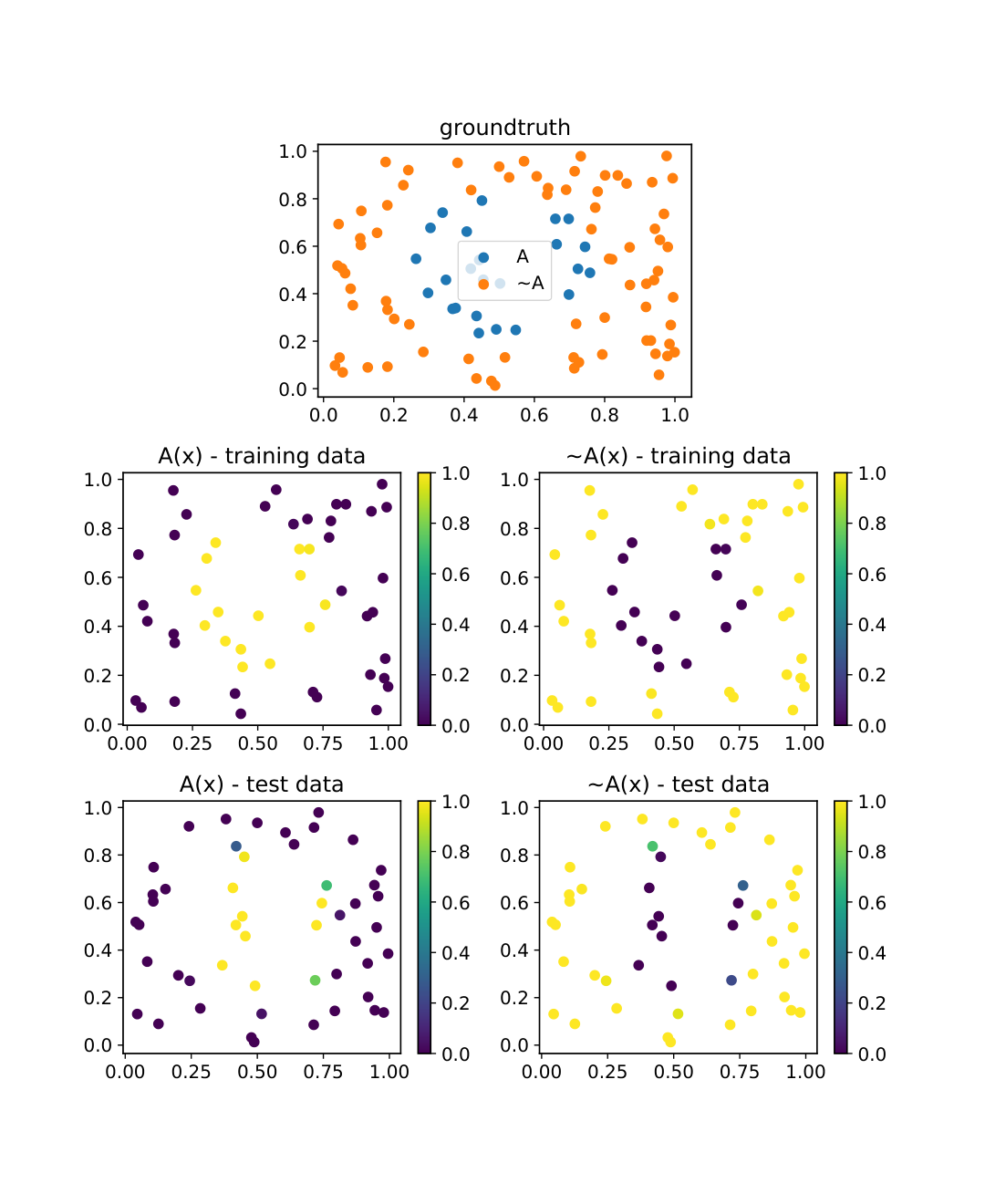
We are therefore interested in learning the parameters $\theta$ of the $\mathtt{MLP}$ used to model the binary classifier. We sample 100 data points uniformly from $[0,1]^{2}$ to populate the data set of positive and negative examples. The data set was split into 50 data points for training and 50 points for testing. The training was carried out for a fixed number of 1000 epochs using backpropagation with the Adam optimizer [35] with a batch size of $64$ examples. Figure 8 shows the classification accuracy and satisfaction level of the LTN on both training and test sets averaged over 10 runs using a 95% confidence interval. The accuracy shown is the ratio of examples correctly classified, with an example deemed as being positive if the classifier outputs a value higher than $0.5$.

Notice that a model can reach an accuracy of $100\%$ while satisfaction of the knowledge base is yet not maximized. For example, if the threshold for an example to be deemed as positive is $0.7$, all examples may be classified correctly with a confidence score of $0.7$. In that case, while the accuracy is already maximized, the satisfaction of $\forall x_{+}A(x_{+})$ would still be $0.7$, and can still improve until the confidence for every sample reaches $1.0$.

This first example, although straightforward, illustrates step-by-step the process of using LTN in a simple setting. Notice that, according to the nomenclature of Section 3.3, measuring accuracy amounts to querying the truth query (respectively, the generalization truth query) $A(x)$ for all the examples of the training set (respectively, test set) and comparing the results with the classification threshold. In Figure 9, we show the results of such queries $A(x)$ after optimization. Next, we show how the LTN language can be used to solve progressively more complex problems by combining learning and reasoning.

Figure 7: Symbolic Tensor Computational Graph for the Binary Classification Example. In the figure, $\mathcal{G}{x_{+}}$ and $\mathcal{G}{x_{-}}$ are inputs to the network $\mathcal{G}_{\theta}(A)$ and the dotted lines indicate the propagation of activation from each input through the network, which produces two outputs.

Figure 8: Binary Classification task (training and test set performance): Average accuracy (left) and satisfiability (right). Due to the random initializations, accuracy and satisfiability start on average at $0.5$ with performance increasing rapidly after a few epochs.

Figure 9: Binary Classification task (querying the trained predicate $A(x)$): It is interesting to see how $A(x)$ could be appropriately named as denoting the inside of the central region shown in the figure, and therefore $\neg A(x)$ represents the outside of the region.

4.2 Multi-Class Single-Label Classification

The natural extension of binary classification is a multi-class classification task. We first approach multi-class single-label classification, which assumes that each example is assigned to one and only one label.

For illustration purposes, we use the Iris flower data set [20], which consists of classification into three mutually exclusive classes; call these $A$, $B$, and $C$. While one could train three unary predicates $A(x)$, $B(x)$ and $C(x)$, it turns out to be more effective if this problem is modeled by a single binary predicate $P(x,l)$, where $l$ is a variable denoting a multi-class label, in this case, classes $A$, $B$ or $C$. This syntax allows one to write statements quantifying over the classes, e.g. $\forall x(\exists l(P(x,l)))$. Since the classes are mutually exclusive, the output layer of the $\mathtt{MLP}$ representing $P(x,l)$ will be a $\mathtt{softmax}$ layer, instead of a $\mathtt{sigmoid}$ function, to ensure the exclusivity constraint on satisfiability scores.. The problem can be specified as follows:

Domains:

$\mathrm{items}$, denoting the examples from the Iris flower data set.
$\mathrm{labels}$, denoting the class labels.

Variables:

$x_{A}$, $x_{B}$, $x_{C}$ for the positive examples of classes $A$, $B$, $C$.
$x$ for all examples.
$\mathbf{D}(x_{A})=\mathbf{D}(x_{B})=\mathbf{D}(x_{C})=\mathbf{D}(x)=\mathrm{items}$.

Constants:

$l_{A}$, $l_{B}$, $l_{C}$, the labels of classes $A$ (Iris setosa), $B$ (Iris virginica), $C$ (Iris versicolor), respectively.
$\mathbf{D}(l_{A})=\mathbf{D}(l_{B})=\mathbf{D}(l_{C})=\mathrm{labels}$.

Predicates:

$P(x,l)$ denoting the fact that item $x$ is classified as $l$.
$\mathbf{D_{in}}(P)=\mathrm{items},\mathrm{labels}$.

Axioms:

$$\forall x_{A} \ P(x_{A},l_{A})$$ (27)

$$\forall x_{B} \ P(x_{B},l_{B})$$ (28)

$$\forall x_{C} \ P(x_{C},l_{C})$$ (29)

Notice that rules about exclusiveness such as $\forall x(P(x,l_{A})\rightarrow(\lnot P(x,l_{B})\wedge\lnot P(x,l_{C})))$ are not included since such constraints are already imposed by the grounding of $P$ below, more specifically the $\mathtt{softmax}$ function.

Grounding:

$\mathcal{G}(\mathrm{items})=\mathbb{R}^{4}$, items are described by $4$ features: the length and the width of the sepals and petals, in centimeters.
$\mathcal{G}(\mathrm{labels})=\mathbb{N}^{3}$, we use a one-hot encoding to represent classes.
$\mathcal{G}(x_{A})\in\mathbb{R}^{m_{1}\times 4}$, that is, $\mathcal{G}(x_{A})$ is a sequence of $m_{1}$ examples of class $A$.
$\mathcal{G}(x_{B})\in\mathbb{R}^{m_{2}\times 4}$, $\mathcal{G}(x_{B})$ is a sequence of $m_{2}$ examples of class $B$.
$\mathcal{G}(x_{C})\in\mathbb{R}^{m_{3}\times 4}$, $\mathcal{G}(x_{C})$ is a sequence of $m_{3}$ examples of class $C$.
$\mathcal{G}(x)\in\mathbb{R}^{(m_{1}+m_{2}+m_{3})\times 4}$, $\mathcal{G}(x)$ is a sequence of all the examples.
$\mathcal{G}(l_{A})=[1,0,0]$, $\mathcal{G}(l_{B})=[0,1,0]$, $\mathcal{G}(l_{C})=[0,0,1]$.
$\mathcal{G}(P\mid\theta):x,l\mapsto l^{\top}\cdot\mathtt{softmax}(\mathtt{MLP}_{\theta}(x))$, where the $\mathtt{MLP}$ has three output neurons corresponding to as many classes, and $\cdot$ denotes the dot product as a way of selecting an output for $\mathcal{G}(P\mid\theta)$; multiplying the $\mathtt{MLP}$’s output by the one-hot vector $l^{\top}$ gives the truth degree corresponding to the class denoted by $l$.

Learning:

The logical operators and connectives are approximated using the stable product configuration with $p=2$ for $A_{pME}$. For the formula aggregator, $A_{pME}$ is used also with $p=2$.
The computational graph of Figure 10 illustrates how $\Sat_{\phi\in\mathcal{K}}\mathcal{G}_{\theta}(\phi)$ is obtained. If $\bm{U}$ denotes batches sampled from the data set of all examples, the loss function (to minimize) is:

$$\bm{L}=1-\Sat_{\phi\in\mathcal{K}}\mathcal{G}_{\theta,x\leftarrow\bm{B}}(\phi).$$

Figure 11 shows the result of training with the Adam optimizer with batches of 64 examples. Accuracy measures the ratio of examples correctly classified, with example $x$ labeled as $\argmax_{l}(P(x,l))$. Classification accuracy reaches an average value near $1.0$ for both the training and test data after some 100 epochs. Satisfaction levels of the Iris flower predictions continue to increase for the rest of the training (500 epochs) to more than $0.8$.

It is worth contrasting the choice of using a binary predicate $(P(x,l))$ in this example with the option of using multiple unary predicates $(l_{A}(x),l_{B}(x),l_{C}(x))$, one for each class. Notice how each predicate is normally associated with an output neuron. In the case of the unary predicates, the networks would be disjoint (or modular), whereas weight-sharing takes place with the use of the binary predicate. Since $l$ is instantiated into $l_{A},l_{B},l_{C}$, in practice $P(x,l)$ becomes $P(x,l_{A})$, $P(x,l_{B})$, $P(x,l_{C})$, which is implemented via three output neurons to which a softmax function applies.

Figure 10: Symbolic Tensor Computational Graph for the Multi-Class Single-Label Problem. As before, the dotted lines in the figure indicate the propagation of activation from each input through the network, in this case producing three outputs.

Figure 11: Multi-Class Single-Label Classification: Classification accuracy (left) and satisfaction level (right).

4.3 Multi-Class Multi-Label Classification

We now turn to multi-label classification, whereby multiple labels can be assigned to each example. As a first example of the reach of LTNs, we shall see how the previous example can be extended naturally using LTN to account for multiple labels, not always a trivial extension for most ML algorithms. The standard approach to the multi-label problem is to provide explicit negative examples for each class. By contrast, LTN can use background knowledge to relate classes directly to each other, thus becoming a powerful tool in the case of the multi-label problem when typically the labeled data is scarce. We explore the Leptograpsus crabs data set [10] consisting of 200 examples of 5 morphological measurements of 50 crabs. The task is to classify the crabs according to their color and sex. There are four labels: blue, orange, male, and female. The color labels are mutually exclusive, and so are the labels for sex. LTN will be used to specify such information logically.

Domains:

$\mathrm{items}$ denoting the examples from the crabs dataset.
$\mathrm{labels}$ denoting the class labels.

Variables:

$x_{\mathrm{blue}}$, $x_{\mathrm{orange}}$, $x_{\mathrm{male}}$, $x_{\mathrm{female}}$ for the positive examples of each class.
$x$, used to denote all the examples.
$\mathbf{D}(x_{\mathrm{blue}})=\mathbf{D}(x_{\mathrm{orange}})=\mathbf{D}(x_{\mathrm{male}})=\mathbf{D}(x_{\mathrm{female}})=\mathbf{D}(x)=\mathrm{items}$.

Constants:

$l_{\mathrm{blue}}$, $l_{\mathrm{orange}}$, $l_{\mathrm{male}}$, $l_{\mathrm{female}}$ (the labels for each class).
$\mathbf{D}(l_{\mathrm{blue}})=\mathbf{D}(l_{\mathrm{orange}})=\mathbf{D}(l_{\mathrm{male}})=\mathbf{D}(l_{\mathrm{female}})=\mathrm{labels}$.

Predicates:

$P(x,l)$, denotes the fact that item $x$ is labelled as $l$.
$\mathbf{D_{in}}(P)=\mathrm{items},\mathrm{labels}$.

Axioms:

$$\forall x_{\mathrm{blue}}\ P(x_{\mathrm{blue}},l_{\mathrm{blue}})$$ (30)

$$\forall x_{\mathrm{orange}}\ P(x_{\mathrm{orange}},l_{\mathrm{orange}})$$ (31)

$$\forall x_{\mathrm{male}}\ P(x_{\mathrm{male}},l_{\mathrm{male}})$$ (32)

$$\forall x_{\mathrm{female}}\ P(x_{\mathrm{female}},l_{\mathrm{female}})$$ (33)

$$\forall x\ \lnot(P(x,l_{\mathrm{blue}})\land P(x,l_{\mathrm{orange}}))$$ (34)

$$\forall x\ \lnot(P(x,l_{\mathrm{male}})\land P(x,l_{\mathrm{female}}))$$ (35)

Notice how logical rules 34 and 35 above represent the mutual exclusion of the labels on colour and sex, respectively. As a result, negative examples are not used explicitly in this specification.

Grounding:

$\mathcal{G}(\mathrm{items})=\mathbb{R}^{5}$; the examples from the data set are described using 5 features.
$\mathcal{G}(\mathrm{labels})=\mathbb{N}^{4}$; one-hot vectors are used to represent class labels.

$\mathcal{G}(x_{\mathrm{blue}})\in\mathbb{R}^{m_{1}\times 5}$, $\mathcal{G}(x_{\mathrm{orange}})\in\mathbb{R}^{m_{2}\times 5}$, $\mathcal{G}(x_{\mathrm{male}})\in\mathbb{R}^{m_{3}\times 5}$, $\mathcal{G}(x_{\mathrm{female}})\in\mathbb{R}^{m_{4}\times 5}$. These sequences are not mutually-exclusive, one example can for instance be in both $x_{\mathrm{blue}}$ and $x_{\mathrm{male}}$.
$\mathcal{G}(l_{\mathrm{blue}})=[1,0,0,0]$, $\mathcal{G}(l_{\mathrm{orange}})=[0,1,0,0]$,$\mathcal{G}(l_{\mathrm{male}})=[0,0,1,0]$,$\mathcal{G}(l_{\mathrm{female}})=[0,0,0,1]$.
$\mathcal{G}(P\mid\theta):x,l\mapsto l^{\top}\cdot\mathtt{sigmoid}(\mathtt{MLP}_{\theta}(x))$, with the $\mathtt{MLP}$ having four output neurons corresponding to as many classes. As before, $\cdot$ denotes the dot product which selects a single output. By contrast with the previous example, notice the use of a $\mathtt{sigmoid}$ function instead of a $\mathtt{softmax}$ function.

Learning:

As before, the fuzzy logic operators and connectives are approximated using the stable product configuration with $p=2$ for $A_{pME}$, and for the formula aggregator, $A_{pME}$ is also used with $p=2$.
Figure 12 shows the result of the Adam optimizer using backpropagation trained with batches of 64 examples. This time, the accuracy is defined as $1-\mathrm{HL}$, where $\mathrm{HL}$ is the average Hamming loss, i.e. the fraction of labels predicted incorrectly, with a classification threshold of $0.5$ (given an example $u$, if the model outputs a value greater than $0.5$ for class $C$ then $u$ is deemed as belonging to class $C$). The rightmost graph in Figure 12 illustrates how LTN learns the constraint that a crab cannot have both blue and orange color, which is discussed in more detail in what follows.

Querying:

To illustrate the learning of constraints by LTN, we have queried three formulas that were not explicitly part of the knowledge-base, over time during learning:

$$\phi_{1} : \forall x\ (P(x,l_{\mathrm{blue}})\rightarrow\lnot P(x,l_{\mathrm{orange}}))$$ (36)

$$\phi_{2} : \forall x\ (P(x,l_{\mathrm{blue}})\rightarrow P(x,l_{\mathrm{orange}}))$$ (37)

$$\phi_{3} : \forall x\ (P(x,l_{\mathrm{blue}})\rightarrow P(x,l_{\mathrm{male}}))$$ (38)

For querying, we use $p=5$ when approximating the universal quantifiers with $A_{pME}$. A higher $p$ denotes a stricter universal quantification with a stronger focus on outliers (see Section 2.4). We should expect $\phi_{1}$ to hold true (every blue crab cannot be orange and vice-versa, and we should expect $\phi_{2}$ (every blue crab is also orange) and $\phi_{3}$ (every blue crab is male) to be false. The results are reported in the rightmost plot of Figure 12. Prior to training, the truth-values of $\phi_{1}$ to $\phi_{3}$ are non-informative. During training one can see, with the maximization of the satisfaction of the knowledge-base, a trend towards the satisfaction of $\phi_{1}$, and an opposite trend of $\phi_{2}$ and $\phi_{3}$ towards false.

Figure 12: Multi-Class Multi-Label Classification: Classification Accuracy (left), Satisfiability level (middle), and Querying of Constraints (right).

4.4 Semi-Supervised Pattern recognition

Let us now explore two, more elaborate, classification tasks, which showcase the benefit of using logical reasoning alongside machine learning. With these two examples, we also aim to provide a more direct comparison with a related neurosymbolic system DeepProbLog [41]. The benchmark examples below were introduced in the DeepProbLog paper [41].

Single Digits Addition:

Consider the predicate $\mathtt{addition(X,Y,N)}$, where $\mathtt{X}$ and $\mathtt{Y}$ are images of digits (the MNIST data set will be used), and $\mathtt{N}$ is a natural number corresponding to the sum of these digits. This predicate should return an estimate of the validity of the addition. For instance, $\mathtt{addition(\raisebox{-1.94444pt}{\includegraphics[height=8.77776pt]{figures/mnist_three.png}},\raisebox{-1.94444pt}{\includegraphics[height=8.77776pt]{figures/mnist_eight.png}},11)}$ is a valid addition; $\mathtt{addition(\raisebox{-1.94444pt}{\includegraphics[height=8.77776pt]{figures/mnist_three.png}},\raisebox{-1.94444pt}{\includegraphics[height=8.77776pt]{figures/mnist_eight.png}},5)}$ is not.

Multi Digits Addition:

The experiment is extended to numbers with more than one digit. Consider the predicate $\mathtt{addition([X_{1},X_{2}],[Y_{1},Y_{2}],N)}$. $\mathtt{[X_{1},X_{2}]}$ and $\mathtt{[Y_{1},Y_{2}]}$ are lists of images of digits, representing two multi-digit numbers; $\mathtt{N}$ is a natural number corresponding to the sum of the two multi-digit numbers. For instance, $\mathtt{addition([\raisebox{-1.94444pt}{\includegraphics[height=8.77776pt]{figures/mnist_three.png}},\raisebox{-1.94444pt}{\includegraphics[height=8.77776pt]{figures/mnist_eight.png}}],[\raisebox{-1.94444pt}{\includegraphics[height=8.77776pt]{figures/mnist_nine.png}},\raisebox{-1.94444pt}{\includegraphics[height=8.77776pt]{figures/mnist_two.png}}],130)}$ is a valid addition; $\mathtt{addition([\raisebox{-1.94444pt}{\includegraphics[height=8.77776pt]{figures/mnist_three.png}},\raisebox{-1.94444pt}{\includegraphics[height=8.77776pt]{figures/mnist_eight.png}}],[\raisebox{-1.94444pt}{\includegraphics[height=8.77776pt]{figures/mnist_nine.png}},\raisebox{-1.94444pt}{\includegraphics[height=8.77776pt]{figures/mnist_two.png}}],26)}$ is not.

A natural neurosymbolic approach is to seek to learn a single-digit classifier and benefit from knowledge readily available about the properties of addition in this case. For instance, suppose that a predicate $\mathrm{digit}(x,d)$ gives the likelihood of an image $x$ being of digit $d$. A definition for $\mathtt{addition(\raisebox{-1.94444pt}{\includegraphics[height=8.77776pt]{figures/mnist_three.png}},\raisebox{-1.94444pt}{\includegraphics[height=8.77776pt]{figures/mnist_eight.png}},11)}$ in LTN is:

$$\exists d_{1},d_{2}:d_{1}+d_{2}=11\ (\mathrm{digit}(\raisebox{-1.94444pt}{\includegraphics[height=8.77776pt]{figures/mnist_three.png}},d_{1})\land\mathrm{digit}(\raisebox{-1.94444pt}{\includegraphics[height=8.77776pt]{figures/mnist_eight.png}},d_{2}))$$

In [41], the above task is made more complicated by not providing labels for the single-digit images during training. Instead, training takes place on pairs of images with labels made available for the result only, that is, the sum of the individual labels. The single-digit classifier is not explicitly trained by itself; its output is a piece of latent information that is used by the logic. However, this does not pose a problem for end-to-end neurosymbolic systems such as LTN or DeepProbLog for which the gradients can propagate through the logical structures.

We start by illustrating a LTN theory that can be used to learn the predicate $\mathrm{digit}$. The specification of the theory below is for the single digit addition example, although it can be extended easily to the multiple digits case.

Domains:

$\mathrm{images}$, denoting the MNIST digit images,
$\mathrm{results}$, denoting the integers that label the results of the additions,
$\mathrm{digits}$, denoting the digits from 0 to 9.

Variables:

$x$, $y$, ranging over the MNIST images in the data,
$n$ for the labels, i.e. the result of each addition,
$d_{1}$, $d_{2}$ ranging over digits.
$\mathbf{D}(x)=\mathbf{D}(y)=\mathrm{images}$,
$\mathbf{D}(n)=\mathrm{results}$,
$\mathbf{D}(d_{1})=\mathbf{D}(d_{2})=\mathrm{digits}$.

Predicates:

$\mathrm{digit}(x,d)$ for the single digit classifier, where $d$ is a term denoting a digit constant or a digit variable. The classifier should return the probability of an image $x$ being of digit $d$.
$\mathbf{D_{in}}(\mathrm{digit})=\mathrm{images},\mathrm{digits}$.

Axioms:

Single Digit Addition:

$$\forall\mathrm{Diag}(x,y,n)$$

$$\quad(\exists d_{1},d_{2}:d_{1}+d_{2}=n$$ (39)

$$\qquad(\mathrm{digit}(x,d_{1})\land\mathrm{digit}(y,d_{2})))$$

Multiple Digit Addition:

$$\forall\mathrm{Diag}(x_{1},x_{2},y_{1},y_{2},n)$$

$$\quad(\exists d_{1},d_{2},d_{3},d_{4}:10d_{1}+d_{2}+10d_{3}+d_{4}=n$$ (40)

$$\qquad(\mathrm{digit}(x_{1},d_{1})\land\mathrm{digit}(x_{2},d_{2})\land\mathrm{digit}(y_{1},d_{3})\land\mathrm{digit}(y_{2},d_{4})))$$

Notice the use of $\mathrm{Diag}$: when grounding $x$,$y$,$n$ with three sequences of values, the $i$-th examples of each variable are matching. That is, $(\mathcal{G}(x)_{i},\mathcal{G}(y)_{i},\mathcal{G}(n)_{i})$ is a tuple from our dataset of valid additions. Using the diagonal quantification, LTN aggregates pairs of images and their corresponding result, rather than any combination of images and results.

Notice also the guarded quantification: by quantifying only on the latent "digit labels" (i.e. $d_{1}$,$d_{2}$, …) that can add up to the result label ($n$, given in the dataset), we incorporate symbolic information into the system. For example, in (39), if $n=3$, the only valid tuples $(d_{1},d_{2})$ are $(0,3),(3,0),(1,2),(2,1)$. Gradients will only backpropagate to these values.

Grounding:

$\mathcal{G}(\mathrm{images})=[0,1]^{28\times 28\times 1}$. The MNIST data set has images of $28$ by $28$ pixels. The images are grayscale and have just one channel. The RGB pixel values from $0$ to $255$ of the MNIST data set are converted to the range $[0,1]$.
$\mathcal{G}(\mathrm{results})=\mathbb{N}$.
$\mathcal{G}(\mathrm{digits})=\{0,1,\dots,9\}$.
$\mathcal{G}(x)\in[0,1]^{m\times 28\times 28\times 1}$, $\mathcal{G}(y)\in[0,1]^{m\times 28\times 28\times 1}$, $\mathcal{G}(n)\in\mathbb{N}^{m}$.
$\mathcal{G}(d_{1})=\mathcal{G}(d_{2})=\left<0,1,\dots,9\right>$.
$\mathcal{G}(\mathrm{digit}\mid\theta):x,d\mapsto\mathtt{onehot}(d)^{\top}\cdot\mathtt{softmax}(\mathtt{CNN}_{\theta}(x))$, where $\mathtt{CNN}$ is a Convolutional Neural Network with $10$ output neurons for each class. Notice that, in contrast with the previous examples, $d$ is an integer label; $\mathtt{onehot}(d)$ converts it into a one-hot label.

Learning:

The computational graph of Figure 13 shows the objective function for the satisfiability of the knowledge base. A stable product configuration is used with hyper-parameter $p=2$ of the operator $A_{pME}$ for universal quantification ($\forall$). Let $p_{\exists}$ denote the exponent hyper-parameter used in the generalized mean $A_{pM}$ for existential quantification ($\exists$). Three scenarios are investigated and compared in the Multiple Digit experiment (Figure 15):

1. $p_{\exists}=1$ throughout the entire experiment,

2. $p_{\exists}=2$ throughout the entire experiment, or

3. $p_{\exists}$ follows a schedule, changing from $p=1$ to $p=6$ gradually with the number of training epochs.

In the Single Digit experiment, only the last scenario above (schedule) is investigated (Figure 14).

We train to maximize satisfiability by using batches of 32 examples of image pairs, labeled by the result of their addition. As done in [41], the experimental results vary the number of examples in the training set to emphasize the generalization abilities of a neurosymbolic approach. Accuracy is measured by predicting the digit values using the predicate $\mathrm{digit}$ and reporting the ratio of examples for which the addition is correct. A comparison is made with the same baseline method used in [41]: given a pair of MNIST images, a non-pre-trained CNN outputs embeddings for each image (Siamese neural network). The embeddings are provided as input to dense layers that classify the addition into one of the 19 (respectively, 199) possible results of the Single Digit Addition (respectively, Multiple Digit Addition) experiments. The baseline is trained using a cross-entropy loss between the labels and the predictions. As expected, such a standard deep learning approach struggles with the task without the provision of symbolic meaning about intermediate parts of the problem.

Experimentally, we find that the optimizer for the neurosymbolic system gets stuck in a local optimum at the initialization in about 1 out of 5 runs. We, therefore, present the results on an average of the 10 best outcomes out of 15 runs of each algorithm (that is, for the baseline as well). The examples of digit pairs selected from the full MNIST data set are randomized at each run.

Figure 15 shows that the use of $p_{\exists}=2$ from the start produces poor results. A higher value for $p_{\exists}$ in $A_{pM}$ weighs up the instances with a higher truth-value (see also C for a discussion). Starting already with a high value for $p_{\exists}$, the classes with a higher initial truth-value for a given example will have higher gradients and be prioritized for training, which does not make practical sense when randomly initializing the predicates. Increasing $p_{\exists}$ by following a schedule is the most promising approach. In this particular example, $p_{\exists}=1$ is also shown to be adequate purely from a learning perspective. However, $p_{\exists}=1$ implements a simple average which does not account for the meaning of $\exists$ well; the resulting satisfaction value is not meaningful within a reasoning perspective.

Table 1 shows that the training and test times of LTN are of the same order of magnitude as those of the CNN baselines. Table 2 shows that LTN reaches similar accuracy as that reported by DeepProbLog.

	(Single Digits)		(Multi Digits)
Model	Train	Test	Train	Test
$\mathrm{baseline}$	$2.72\pm 0.23\mathrm{ms}$	$1.45\pm 0.21\mathrm{ms}$	$3.87\pm 0.24\mathrm{ms}$	$2.10\pm 0.30\mathrm{ms}$
$\mathrm{LTN}$	$5.36\pm 0.25\mathrm{ms}$	$3.44\pm 0.39\mathrm{ms}$	$8.51\pm 0.72\mathrm{ms}$	$5.72\pm 0.57\mathrm{ms}$

Table 1: The computation time of training and test steps on the single and multiple digit addition tasks, measured on a computer with a single Nvidia Tesla V100 GPU and averaged over 1000 steps. Each step operates on a batch of 32 examples. The computational efficiency of the LTN and the CNN baseline systems are of the same order of magnitude.

	Number of training examples
	(Single Digits)		(Multi Digits)
Model	30 000	3 000	15 000	1 500
$\mathrm{baseline}$	$95.95\pm 0.27$	$70.59\pm 1.45$	$47.19\pm 0.69$	$2.07\pm 0.12$
$\mathrm{LTN}$	$98.04\pm 0.13$	$93.49\pm 0.28$	$95.37\pm 0.29$	$88.21\pm 0.63$
$\mathrm{DeepProbLog}$	$97.20\pm 0.45$	$92.18\pm 1.57$	$95.16\pm 1.70$	$87.21\pm 1.92$

Table 2: Accuracy (in %) on the test set: comparison of the final results obtained with LTN and those reported with DeepProbLog[41]. Although it is difficult to compare directly the results over time (the frameworks are implemented in different libraries), while achieving similar computational efficiency as the CNN baseline, LTN also reaches similar accuracy as that reported by DeepProbLog.

Figure 13: Symbolic Tensor Computational Graph for the Single Digit Addition task. Notice that the figure does not depict accurate dimensions for the tensors; $\mathcal{G}(x)$ and $\mathcal{G}(y)$ are in fact 4D tensors of dimensions $m\times 28\times 28\times 1$. Computing results with the variables $d_{1}$ or $d_{2}$ corresponds to the addition of a further axes of dimension $10$.

Figure 14: Single Digit Addition Task: Accuracy and satisfiability results (top) and results in the presence of fewer examples (bottom) in comparison with standard Deep Learning using a CNN (blue lines).

Figure 15: Multiple Digit Addition Task: Accuracy and satisfiability results (top) and results in the presence of fewer examples (bottom) in comparison with standard Deep Learning using a CNN (blue lines).

4.5 Regression

Another important problem in Machine Learning is regression where a relationship is estimated between one independent variable $X$ and a continuous dependent variable $Y$. The essence of regression is, therefore, to approximate a function $f(x)=y$ by a function $f^{*}$, given examples $(x_{i},y_{i})$ such that $f(x_{i})=y_{i}$. In LTN one can model a regression task by defining $f^{*}$ as a learnable function whose parameter values are constrained by data. Additionally, a regression task requires a notion of equality. We, therefore, define the predicate $\mathrm{eq}$ as a smooth version of the symbol $=$ to turn the constraint $f(x_{i})=y_{i}$ into a smooth optimization problem.

In this example, we explore regression using a problem from a real estate data set with 414 examples, each described in terms of 6 real-numbered features: the transaction date (converted to a float), the age of the house, the distance to the nearest station, the number of convenience stores in the vicinity, and the latitude and longitude coordinates. The model has to predict the house price per unit area.

Domains:

$\mathrm{samples}$, denoting the houses and their features.
$\mathrm{prices}$, denoting the house prices.

Variables:

$x$ for the samples.
$y$ for the prices.
$\mathbf{D}(x)=\mathrm{samples}$.
$\mathbf{D}(y)=\mathrm{prices}$.

Functions:

$f^{*}(x)$, the regression function to be learned.
$\mathbf{D_{in}}(f^{*})=\mathrm{samples}$, $\mathbf{D_{out}}(f^{*})=\mathrm{prices}$.

Predicates:

$\mathrm{eq}(y_{1},y_{2})$, a smooth equality predicate that measures how similar $y_{1}$ and $y_{2}$ are.
$\mathbf{D_{in}}(\mathrm{eq})=\mathrm{prices},\mathrm{prices}$.

Axioms:

$$\forall\mathrm{Diag}(x,y)\ \mathrm{eq}(f^{*}(x),y)$$ (41)

Notice again the use of $\mathrm{Diag}$: when grounding $x$ and $y$ onto sequences of values, this is done by obeying a one-to-one correspondence between the sequences. In other words, we aggregate pairs of corresponding $\mathrm{samples}$ and $\mathrm{prices}$, instead of any combination thereof.

Grounding:

$\mathcal{G}(\mathrm{samples})=\mathbb{R}^{6}$.
$\mathcal{G}(\mathrm{prices})=\mathbb{R}$.
$\mathcal{G}(x)\in\mathbb{R}^{m}\times 6$, $\mathcal{G}(y)\in\mathbb{R}^{m}\times 1$. Notice that this specification refers to the same number $m$ of examples for $x$ and $y$ due to the above one-to-one correspondence obtained with the use of $\mathrm{Diag}$.
$\mathcal{G}(\mathrm{eq}(\mathbf{u},\mathbf{v}))=\exp\big(-\alpha\sqrt{\sum_{j}(u_{j}-v_{j})^{2}}\big)$, where the hyper-parameter $\alpha$ is a real number that scales how strict the smooth equality is. In our experiments, we use $\alpha=0.05$.
$\mathcal{G}(f^{*}(x)\mid\theta)=\mathtt{MLP}_{\theta}(x)$, where $\mathtt{MLP}_{\theta}$ is a multilayer perceptron which ends in one neuron corresponding to a price prediction, with a linear output layer (no activation function).

Learning:

The theory is constrained by the parameters of the model of $f^{*}$. LTN is used to estimate such parameters by maximizing the satisfaction of the knowledge-base, in the usual way. Approximating $\forall$ using $A_{pME}$ with $p=2$, as before, we randomly split the data set into 330 examples for training and 84 examples for testing. Figure 16 shows the satisfaction level over 500 epochs. We also plot the Root Mean Squared Error (RMSE) between the predicted prices and the labels (i.e. actual prices, also known as target values). We visualize in Figure 17 the strong correlation between actual and predicted prices at the end of one of the runs.

Figure 16: Regression task: RMSE and satisfaction level over time.

Figure 17: Visualization of LTN solving a regression problem.

4.6 Unsupervised Learning (Clustering)

In unsupervised learning, labels are either not available or are not used for learning. Clustering is a form of unsupervised learning whereby, without labels, the data is characterized by constraints alone. LTN can formulate such constraints, such as:

• clusters should be disjoint,

• every example should be assigned to a cluster,

• a cluster should not be empty,

• if the points are near, they should belong to the same cluster,

• if the points are far, they should belong to different clusters, etc.

Domains:

$\mathrm{points}$, denoting the data to cluster.
$\mathrm{points\_pairs}$, denoting pairs of examples.
$\mathrm{clusters}$, denoting the cluster.

Variables:

$x$, $y$ for all points.
$\mathbf{D}(x)=\mathbf{D}(y)=\mathrm{points}$.
$\mathbf{D}(c)=\mathrm{clusters}$.

Predicates:

$C(x,c)$, the truth degree of a given point belonging in a given cluster.
$\mathbf{D_{in}}(C)=\mathrm{points},\mathrm{clusters}$.

Axioms:

$$\forall x \ \exists c\ C(x,c)$$ (42)

$$\forall c \ \exists x\ C(x,c)$$ (43)

$$\forall(c,x,y:\lvert x-y\rvert<\mathrm{th_{close}}) \ \ (C(x,c)\leftrightarrow C(y,c))$$ (44)

$$\forall(c,x,y:\lvert x-y\rvert>\mathrm{th_{distant}}) \ \ \lnot(C(x,c)\land C(y,c))$$ (45)

Notice the use of guarded quantifiers: all the pairs of points with Euclidean distance lower (resp. higher) than a value $\mathrm{th_{close}}$ (resp. $\mathrm{th_{distant}}$) should belong in the same cluster (resp. should not). $\mathrm{th_{close}}$ and $\mathrm{th_{distant}}$ are arbitrary threshold values that define some of the closest and most distant pairs of points. In our example, they are set to, respectively, $0.2$ and $1.0$.
As done in the example of Section 4.2, the clustering predicate has mutually exclusive satisfiability scores for each cluster using a $\mathtt{softmax}$ layer. Therefore, there is no explicit constraint about clusters being disjoint.

Grounding:

$\mathcal{G}(\mathrm{points})=[-1,1]^{2}$.
$\mathcal{G}(\mathrm{clusters})=\mathbb{N}^{4}$, we use one-hot vectors to represent a choice of 4 clusters.
$\mathcal{G}(x)\in[-1,1]^{m\times 2}$, that is, $x$ is a sequence of $m$ points. $\mathcal{G}(y)=\mathcal{G}(x)$.
$\mathrm{th_{close}}=0.2$, $\mathrm{th_{distant}}=1.0$.
$\mathcal{G}(c)=\left<[1,0,0,0],[0,1,0,0],[0,0,1,0],[0,0,0,1]\right>$.
$\mathcal{G}(C\mid\theta):x,c\mapsto c^{\top}\cdot\mathtt{softmax}(\mathtt{MLP}_{\theta}(x))$, where $\mathtt{MLP}$ has 4 output neurons corresponding to the 4 clusters.

Learning:

We use the stable real product configuration to approximate the logical operators. For $\forall$, we use $A_{pME}$ with $p=4$. For $\exists$, we use $A_{pM}$ with $p=1$ during the first 100 epochs, and $p=6$ thereafter, as a simplified version of the schedule used in Section 4.4. The formula aggregator is approximated by $A_{pME}$ with $p=2$. The model is trained for a total of 1000 epochs using the Adam optimizer, which is sufficient for LTN to solve the clustering problem shown in Figure 18. Ground-truth data for this task was generated artificially by creating 4 centers, and generating $50$ random samples from a multivariate Gaussian distribution around each center. The trained LTN achieves a satisfaction level of the clustering constraints of $0.857$.

Figure 18: LTN solving a clustering problem by constraint optimization: ground-truth (top) and querying of each cluster $C0$, $C1$, $C2$ and $C3$, in turn.

4.7 Learning Embeddings with LTN

A classic example of Statistical Relational Learning is the smokers-friends-cancer example introduced in [55]. Below, we show how this example can be formalized in LTN using semi-supervised embedding learning.

There are 14 people divided into two groups $\{a,b,\dots,h\}$ and $\{i,j,\dots,n\}$. Within each group, there is complete knowledge about smoking habits. In the first group, there is complete knowledge about who has and who does not have cancer. Knowledge about the friendship relation is complete within each group only if symmetry is assumed, that is, $\forall x,y\ (friends(x,y)\rightarrow friends(y,x))$. Otherwise, knowledge about friendship is incomplete in that it may be known that e.g. $a$ is a friend of $b$, and it may be not known whether $b$ is a friend of $a$. Finally, there is general knowledge about smoking, friendship, and cancer, namely that smoking causes cancer, friendship is normally symmetric and anti-reflexive, everyone has a friend, and smoking propagates (actively or passively) among friends. All this knowledge is represented in the axioms further below.

Domains:

$\mathrm{people}$, to denote the individuals.

Constants:

$a,b,\dots,h,i,j,\dots,n$, the 14 individuals. Our goal is to learn an adequate embedding for each constant.
$\mathbf{D}(a)=\mathbf{D}(b)=\dots=\mathbf{D}(n)=\mathrm{people}$.

Variables:

$x$,$y$ ranging over the individuals.
$\mathbf{D}(x)=\mathbf{D}(y)=\mathrm{people}$.

Predicates:

$S(x)$ for smokes, $F(x,y)$ for friends, $C(x)$ for cancer.
$\mathbf{D}(S)=\mathbf{D}(C)=\mathrm{people}$. $\mathbf{D}(F)=\mathrm{people},\mathrm{people}$.

Axioms:

Let $\mathcal{X}_{1}=\{a,b,\dots,h\}$ and $\mathcal{X}_{2}=\{i,j,\dots,n\}$ be the two groups of individuals.
Let $\mathcal{S}=\{a,e,f,g,j,n\}$ be the smokers; knowledge is complete in both groups.
Let $\mathcal{C}=\{a,e\}$ be the individuals with cancer; knowledge is complete in $\mathcal{X}_{1}$ only.
Let $\mathcal{F}=\{(a,b),(a,e),(a,f),(a,g),(b,c),(c,d),(e,f),(g,h),(i,j),(j,m),(k,l),(m,n)\}$ be the set of friendship relations; knowledge is complete if assuming symmetry.
These facts are illustrated in Figure 20(a).
We have the following axioms:

$$F(u,v) \text{for }(u,v)\in\mathcal{F}$$ (46)

$$\lnot F(u,v) \text{for }(u,v)\notin\mathcal{F},\ u>v$$ (47)

$$S(u) \text{for }u\in\mathcal{S}$$ (48)

$$\lnot S(u) \text{for }u\in(\mathcal{X}_{1}\cup\mathcal{X}_{2})\setminus\mathcal{S}$$ (49)

$$C(u) \text{for }u\in\mathcal{C}$$ (50)

$$\lnot C(u) \text{for }u\in\mathcal{X}_{1}\setminus\mathcal{C}$$ (51)

$$\forall x\ \lnot F(x,x)$$ (52)

$$\forall x,y\ (F(x,y)\rightarrow F(y,x))$$ (53)

$$\forall x\exists y\ F(x,y)$$ (54)

$$\forall x,y\ ((F(x,y)\land S(x))\rightarrow S(y))$$ (55)

$$\forall x\ (S(x)\rightarrow C(x))$$ (56)

$$\forall x\ (\lnot C(x)\rightarrow\lnot S(x))$$ (57)

Notice that the knowledge base is not satisfiable in the strict logical sense of the word. For instance, $f$ is said to smoke but not to have cancer, which is inconsistent with the rule $\forall x\ (S(x)\rightarrow C(x))$. Hence, it is important to adopt a fuzzy approach as done with MLN or a many-valued fuzzy logic interpretation as done with LTN.

Grounding:

$\mathcal{G}(\mathrm{people})=\mathbb{R}^{5}$. The model is expected to learn embeddings in $\mathbb{R}^{5}$.
$\mathcal{G}(a\mid\theta)=\mathbf{v}_{\theta}(a)$, …, $\mathcal{G}(n\mid\theta)=\mathbf{v}_{\theta}(n)$. Every individual is associated with a vector of 5 real numbers. The embedding is initialized randomly uniformly.
$\mathcal{G}(x\mid\theta)=\mathcal{G}(y\mid\theta)=\left<\mathbf{v}_{\theta}(a),\dots,\mathbf{v}_{\theta}(n)\right>$.
$\mathcal{G}(S\mid\theta):x\mapsto\mathtt{sigmoid}(\mathtt{MLP\_S}_{\theta}(x))$, where $\mathtt{MLP\_S}_{\theta}$ has 1 output neuron.
$\mathcal{G}(F\mid\theta):x,y\mapsto\mathtt{sigmoid}(\mathtt{MLP\_F}_{\theta}(x,y))$, where $\mathtt{MLP\_F}_{\theta}$ has 1 output neuron.
$\mathcal{G}(C\mid\theta):x\mapsto\mathtt{sigmoid}(\mathtt{MLP\_C}_{\theta}(x))$, where $\mathtt{MLP\_C}_{\theta}$ has 1 output neuron.
The $\mathtt{MLP}$ models for $S$, $F$, $C$ are kept simple, so that most of the learning is focused on the embedding.

Learning:

We use the stable real product configuration to approximate the operators. For $\forall$, we use $A_{pME}$ with $p=2$ for all the rules, except for rules (52) and (53), where we use $p=6$. The intuition behind this choice of $p$ is that no outliers are to be accepted for the friendship relation since it is expected to be symmetric and anti-reflexive, but outliers are accepted for the other rules. For $\exists$, we use $A_{pM}$ with $p=1$ during the first 200 epochs of training, and $p=6$ thereafter, with the same motivation as that of the schedule used in Section 4.4. The formula aggregator is approximated by $A_{pME}$ with $p=2$.

Figure 19 shows the satisfiability over 1000 epochs of training. At the end of one of these runs, we query $S(x)$, $F(x,y)$, $C(x)$ for each individual; the results are shown in Figure 20(b). We also plot the principal components of the learned embeddings [51] in Figure 21. The friendship relations are learned as expected: (56) "smoking implies cancer" is inferred for group 2 even though such information was not present in the knowledge base. For group 1, the given facts for smoking and cancer for the individuals $f$ and $g$ are slightly altered, as these were inconsistent with the rules. (the rule for smoking propagating via friendship (55) is incompatible with many of the given facts). Increasing the satisfaction of this rule would require decreasing the overall satisfaction of the knowledge base, which explains why it is partly ignored by LTN during training. Finally, it is interesting to note that the principal components for the learned embeddings seem to be linearly separable for the smoking and cancer classifiers (c.f. Figure 21, top right and bottom right plots).

Querying:

To illustrate querying in LTN, we query over time two formulas that are not present in the knowledge-base:

$$\phi_{1} : \forall p: C(p)\rightarrow S(p)$$ (58)

$$\phi_{2} : \forall p,q: (C(p)\lor C(q))\rightarrow F(p,q)$$ (59)

We use $p=5$ when approximating $\forall$ since the impact of an outlier at querying time should be seen as more important than at learning time. It can be seen that as the grounding approaches satisfiability of the knowledge-base, $\phi_{1}$ approaches true, whereas $\phi_{2}$ approaches false (c.f. Figure 20(a)).

Figure 19: Smoker-Friends-Cancer example: Satisfiability levels during training (left) and truth-values of queries $\phi_{1}$ and $\phi_{2}$ over time (right).

(a) Incomplete facts in the knowledge-base: axioms for smokers and cancer for individuals $a$ to $n$ (left), friendship relations in group 1 (middle), and friendship relations in group 2 (right).

(b) Querying all the truth-values using LTN after training: smokers and cancer (left), friendship relations (middle and right).

Figure 20: Smoker-Friends-Cancer example: Illustration of the facts before and after training.

Figure 21: Smoker-Friends-Cancer example: learned embeddings showing the result of applying PCA on the individuals (top left); truth-values of smokes and cancer predicates for each embedding (top and bottom right); illustration of the friendship relations which are satisfied after learning (bottom left).

4.8 Reasoning in LTN

The essence of reasoning is to find out if a closed formula $\phi$ is the logical consequence of a knowledge-base $(\mathcal{K},\mathcal{G}_{\theta},\Theta)$. Section 3.4 introduced two approaches to this problem in LTN:

• By simply querying after learning one seeks to verify if for the grounded theories that maximally satisfy $\mathcal{K}$, the grounding of $\phi$ gives a truth-value greater than a threshold $q$. This often requires checking an infinite number of groundings. Instead, the user approximates the search for these grounded theories by running the optimization a fixed number of times only.

• Reasoning by refutation one seeks to find out a counter-example: a grounding that satisfies the knowledge-base $\mathcal{K}$ but not the formula $\phi$ given the threshold $q$. A search is performed here using a different objective function.

We now demonstrate that reasoning by refutation is the preferred option using a simple example where we seek to find out whether $(A\lor B)\models_{q}A$.

Propositional Variables:

The symbols $A$ and $B$ denote two propositionial variables.

Axioms:

$$A\lor B$$ (60)

Grounding:

$\mathcal{G}(A)=a$, $\mathcal{G}(B)=b$, where $a$ and $b$ are two real-valued parameters. The set of parameters is therefore $\theta=\{a,b\}$. At initialization, $a=b=0$.
We use the probabilistic-sum $S_{P}$ to approximate $\lor$, resulting in the following satisfiability measure:

$$\mathcal{G}_{\theta}(\mathcal{K})=\mathcal{G}_{\theta}(A\lor B)=a+b-ab.$$ (61)

There are infinite global optima maximizing the satisfiability of the theory, as any $\mathcal{G}_{\theta}$ such that $\mathcal{G}_{\theta}(A)=1$ (resp. $\mathcal{G}_{\theta}(B)=1$) gives a satisfiability $\mathcal{G}_{\theta}(\mathcal{K})=1$ for any value of $\mathcal{G}_{\theta}(B)$ (resp. $\mathcal{G}_{\theta}(A)$). As expected, the following groundings are examples of global optima:

1. $\mathcal{G}_{1}(A)=1$, $\mathcal{G}_{1}(B)=1$, $\mathcal{G}_{1}(\mathcal{K})=1$,

2. $\mathcal{G}_{2}(A)=1$, $\mathcal{G}_{2}(B)=0$, $\mathcal{G}_{2}(\mathcal{K})=1$,

3. $\mathcal{G}_{3}(A)=0$, $\mathcal{G}_{3}(B)=1$, $\mathcal{G}_{3}(\mathcal{K})=1$.

Reasoning:

$(A\lor B)\models_{q}A$? That is, given the threshold $q=0.95$, does every $\mathcal{G}_{\theta}$ such that $\mathcal{G}_{\theta}(\mathcal{K})\geq q$ verify $\mathcal{G}_{\theta}(\phi)\geq q$. Immediately, one can notice that this is not the case. For instance, the grounding $\mathcal{G}_{3}$ is a counter-example.

If one simply reasons by querying multiple groundings after learning with the usual objective $\argmax_{(\mathcal{G}_{\theta})}\mathcal{G}_{\theta}(\mathcal{K})$, the results will all converge to $\mathcal{G}_{1}$: $\frac{\partial\mathcal{G}_{\theta}(\mathcal{K})}{\partial a}=1-b$ and $\frac{\partial\mathcal{G}_{\theta}(\mathcal{K})}{\partial b}=1-a$. Every run of the optimizer will increase $a$ and $b$ simultaneously until they reach the optimum $a=b=1$. Because the grid search always converges to the same point, no counter-example is found and the logical consequence is mistakenly assumed true. This is illustrated in Figure 22.

Reasoning by refutation, however, the objective function has an incentive to find a counter-example with $\neg A$, as illustrated in Figure 23. LTN converges to the optimum $\mathcal{G}_{3}$, which refutes the logical consequence.

Figure 22: Querying after learning: 10 runs of the optimizer with objective $\mathcal{G}^{*}=\argmax_{\mathcal{G}_{\theta}}(\mathcal{G}_{\theta}(\mathcal{K}))$. All runs converge to the optimum $\mathcal{G}_{1}$; the grid search misses the counter-example.

Figure 23: Reasoning by refutation: one run of the optimizer with objective $\mathcal{G}^{*}=\argmin_{\mathcal{G}_{\theta}}(\mathcal{G}_{\theta}(\phi)+\mathtt{elu}(\alpha,\beta(q-\mathcal{G}_{\theta}(\mathcal{K})))$, $q=0.95$, $\alpha=0.05$, $\beta=10$. In the first training epochs, the directed search prioritizes the satisfaction of the knowledge base. Then, the minimization of $\mathcal{G}_{\theta}(\phi)$ starts to weigh in more and the search focuses on finding a counter-example. Eventually, the run converges to the optimum $\mathcal{G}_{3}$, which refutes the logical consequence.

5 Related Work

The past years have seen considerable work aiming to integrate symbolic systems and neural networks. We shall focus on work whose objective is to build computational models that integrate deep learning and logical reasoning into a so-called end-to-end (fully differentiable) architecture. We summarize a categorization in Figure 24 where the class containing LTN is further expanded into three sub-classes. The sub-class highlighted in red is the one that contains LTN. The reason why one may wish to combine symbolic AI and neural networks into a neurosymbolic AI system may vary, c.f. [17] for a recent comprehensive overview of approaches and challenges for neurosymbolic AI.

5.1 Neural architectures for logical reasoning

These use neural networks to perform (probabilistic) inference on logical theories. Early work in this direction has shown correspondences between various logical-symbolic systems and neural network models [27, 32, 52, 63, 65]. They have also highlighted the limits of current neural networks as models for knowledge representation. In a nutshell, current neural networks (including deep learning) have been shown capable of representing propositional logic, nonmonotonic logic programming, propositional modal logic, and fragments of first-order logic, but not full first-order or higher-order logic. Recently, there has been a resurgence of interest in the topic with many proposals emerging [13, 48, 53]. In [13], each clause of a Stochastic Logic Program is converted into a factor graph with reasoning becoming differentiable so that it can be implemented by deep networks. In [49], a differentiable unification algorithm is introduced with theorem proving sought to be carried out inside the neural network. Furthermore, in [11, 49] neural networks are used to learn reasoning strategies and logical rule induction.

Reasoning with LTN (Section 3.4) is reminiscent of this category, given that knowledge is not represented in a traditional logical language but in Real Logic.

5.2 Logical specification of neural network architectures

Here the goal is to use a logical language to specify the architecture of a neural network. Examples include [13, 24, 26, 56, 66]. In [26], the languages of extended logic programming (logic programs with negation by failure) and answer set programming are used as background knowledge to set up the initial architecture and set of weights of a recurrent neural network, which is subsequently trained from data using backpropagation. In [24], first-order logic programs in the form of Horn clauses are used to define a neural network that can solve Inductive Logic Programming tasks, starting from the most specific hypotheses covering the set of examples. Lifted relational neural networks [66] is a declarative framework where a Datalog program is used as a compact specification of a diverse range of existing advanced neural architectures, with a particular focus on Graph Neural Networks (GNNs) and their generalizations. In [56] a weighted Real Logic is introduced and used to specify neurons in a highly modular neural network that resembles a tree structure, whereby neurons with different activation functions are used to implement the different logic operators.

To some extent, it is also possible to specify neural architectures using logic in LTN. For example, a user can define a classifier $P(x,y)$ as the formula $P(x,y)=(Q(x,y)\land R(y))\lor S(x,y)$. $\mathcal{G}(P)$ becomes a computational graph that combines the sub-architectures $\mathcal{G}(Q)$, $\mathcal{G}(R)$, and $\mathcal{G}(S)$ according to the syntax of the logical formula.

5.3 Neurosymbolic architectures for the integration of inductive learning and deductive reasoning

These architectures seek to enable the integration of inductive and deductive reasoning in a unique fully differentiable framework [15, 23, 41, 46, 47]. The systems that belong to this class combine a neural component with a logical component. The former consists of one or more neural networks, the latter provides a set of algorithms for performing logical tasks such as model checking, satisfiability, and logical consequence. These two components are tightly integrated so that learning and inference in the neural component are influenced by reasoning in the logical component and vice versa. Logic Tensor Networks belong to this category. Neurosymbolic architectures for integrating learning and reasoning can be further separated into three sub-classes:

1. Approaches that introduce additional layers to the neural network to encode logical constraints which modify the predictions of the network. This sub-class includes Deep Logic Models [46] and Knowledge Enhanced Neural Networks [15].

2. Approaches that integrate logical knowledge as additional constraints in the objective function or loss function used to train the neural network (LTN and [23, 33, 47]).

3. Approaches that apply (differentiable) logical inference to compute the consequences of the predictions made by a set of base neural networks. Examples of this sub-class are DeepProblog [41] and Abductive Learning [14].

Figure 24: Three classes of neurosymbolic approaches with Architectures Integrating Learning and Reasoning further sub-divided into three sub-classes, with LTN belonging to the sub-class highlighted in red.

In what follows, we revise recent neurosymbolic architectures in the same class as LTN: Integrating learning and reasoning.

Systems that modify the predictions of a base neural network:

Among the approaches that modify the predictions of the neural network using logical constraints are Deep Logic Models [46] and Knowledge Enhanced Neural Networks [15]. Deep Logic Models (DLM) are a general architecture for learning with constraints. Here, we will consider the special case where constraints are expressed by logical formulas. In this case, a DLM predicts the truth-values of a set of $n$ ground atoms of a domain $\Delta=\{a_{1},\dots,a_{k}\}$. It consists of two models: a neural network $f(\bm{x}\mid\bm{w})$ which takes as input the features $\bm{x}$ of the elements of $\Delta$ and produces as output an evaluation $\bm{f}$ for all the ground atoms, i.e. $\bm{f}\in[0,1]^{n}$, and a probability distribution $p(\bm{y}\mid\bm{f},\bm{\lambda})$ which is modeled by an undirected graphical model of the exponential family with each logical constraint characterized by a clique that contains the ground atoms, rather similarly to GNNs. The model returns the assignment to the atoms that maximize the weighted truth-value of the constraints and minimize the difference between the prediction of the neural network and a target value $\bm{y}$. Formally:

$$\text{DLM}(\bm{x}\mid\bm{\lambda},\bm{w})=\argmax_{\bm{y}}\left(\sum_{c}\lambda_{c}\Phi_{c}(\bm{y}_{c})-\frac{1}{2}||\bm{y}-\bm{f}(\bm{x}\mid\bm{w})||^{2}\right)$$

Each $\Phi_{c}(\bm{y}_{c})$ corresponds to a ground propositional formula which is evaluated w.r.t. the target truth assignment $\bm{y}$, and $\lambda_{c}$ is the weight associated with formula $\Phi_{c}$. Intuitively, the upper model (the undirected graphical model) should modify the prediction of the lower model (the neural network) minimally to satisfy the constraints. $\bm{f}$ and $\bm{y}$ are truth-values of all the ground atoms obtained from the constraints appearing in the upper model in the domain specified by the data input.

Similar to LTN, DLM evaluates constraints using fuzzy semantics. However, it considers only propositional connectives, whereas universal and existential quantifiers are supported in LTN.

Inference in DLM requires maximizing the prediction of the model, which might be prohibitive in the presence of a large number of instances. In LTN, inference involves only a forward pass through the neural component which is rather simple and can be carried out in parallel. However, in DLM the weight associated with constraints can be learned, while in LTN they are specified in the background knowledge.

The approach taken in Knowledge Enhanced Neural Networks (KENN) [15] is similar to that of DLM. Starting from the predictions $\bm{y}=f_{nn}(\bm{x}\mid\bm{w})$ made by a base neural network $f_{nn}(\cdot\mid\bm{w})$, KENN adds a knowledge enhancer, which is a function that modifies $\bm{y}$ based on a set of weighted constraints formulated in terms of clauses. The formal model can be specified as follows:

$$\text{KENN}(\bm{x}\mid\bm{\lambda},\bm{w})=\sigma(f^{\prime}_{nn}(\bm{x}\mid\bm{w})+\sum_{c}\lambda_{c}\cdot(\mathrm{softmax}(\mathrm{sign}(c)\odot f^{\prime}_{nn}(\bm{x}\mid\bm{w}))\odot\mathrm{sign}(c)))$$

where $f^{\prime}_{nn}(\bm{x}\mid\bm{w})$ are the pre-activations of $f_{nn}(\bm{x}\mid\bm{w})$, $\mathrm{sign}(c)$ is a vector of the same dimension of $\bm{y}$ containing $1,-1$ and $-\infty$, such that $\mathrm{sign}(c)_{i}=1$ (resp. $\mathrm{sign}(c)_{i}=-1$) if the $i$-th atom occurs positively (resp. negatively) in $c$, or $-\infty$ otherwise, and $\odot$ is the element-wise product. KENN learns the weights $\bm{\lambda}$ of the clauses in the background knowledge and the base network parameters $\bm{w}$ by minimizing some standard loss, (e.g. cross-entropy) on a set of training data. If the training data is inconsistent with the constraint, the weight of the constraint will be close to zero. This intuitively implies that the latent knowledge present in the data is preferred to the knowledge specified in the constraints. In LTN, instead, training data and logical constraints are represented uniformly with a formula, and we require that they are both satisfied. A second difference between KENN and LTN is the language: while LTN supports constraints written in full first-order logic, constraints in KENN are limited to universally quantified clauses.

Systems that add knowledge to a neural network by adding a term to the loss function:

In [33], a framework is proposed that learns simultaneously from labeled data and logical rules. The proposed architecture is made of a student network $f_{nn}$ and a teacher network, denoted by $q$. The student network is trained to do the actual predictions, while the teacher network encodes the information of the logical rules. The transfer of information from the teacher to the student network is done by defining a joint loss $\mathscr{L}$ for both networks as a convex combination of the loss of the student and the teacher. If $\tilde{\bm{y}}=f_{nn}(\bm{x}\mid\bm{w})$ is the prediction of the student network for input $\bm{x}$, the loss is defined as:

$$(1-\pi)\cdot\mathscr{L}(\bm{y},\tilde{\bm{y}})+\pi\cdot\mathscr{L}(q(\tilde{\bm{y}}\mid\bm{x}),\tilde{\bm{y}})$$

where $q(\tilde{\bm{y}}\mid\bm{x})=\exp\left(-\sum_{c}\lambda_{c}(1-\phi_{c}(\bm{x},\tilde{\bm{y}}))\right)$ measures how much the predictions $\tilde{\bm{y}}$ satisfy the constraints encoded in the set of clauses $\{\lambda_{c}:\phi_{c}\}_{c\in C}$. Training is iterative. At every iteration, the parameters of the student network are optimized to minimize the loss that takes into account the feedback of the teacher network on the predictions from the previous step. The main difference between this approach and LTN is how the constraints are encoded in the loss. LTN integrates the constraints in the network and optimizes directly their satisfiability with no need for additional training data. Furthermore, the constraints proposed in [33] are universally quantified formulas only.

The approach adopted by Lyrics [47] is analogous to the first version of LTN [61]. Logical constraints are translated into a loss function that measures the (negative) satisfiability level of the network. Differently from LTN, formulas in Lyrics can be associated with weights that are hyper-parameters. In [47], a logarithmic loss function is also used when the product t-norm is adopted. Notice that weights can also be added (indirectly) to LTN by introducing a $0$-ary predicate $p_{w}$ to represent a constraint of the form $p_{w}\wedge\phi$. An advantage of this approach would be that the weights could be learned.

In [72], a neural network computes the probability of some events being true. The neural network should satisfy a set of propositional logic constraints on its output. These constraints are compiled into arithmetic circuits for weighted model counting, which are then used to compute a loss function. The loss function then captures how close the neural network is to satisfying the propositional logic constraints.

Systems that apply logical reasoning on the predictions of a base neural network:

The most notable architecture in this category is DeepProblog [41]. DeepProblog extends the ProbLog framework for probabilistic logic programming to allow the computation of probabilistic evidence from neural networks. A ProbLog program is a logic program where facts and rules can be associated with probability values. Such values can be learned. Inference in ProbLog to answer a query $q$ is performed by knowledge compilation into a function $p(q\mid\bm{\lambda})$ that computes the probability that $q$ is true according to the logic program with relative frequencies $\bm{\lambda}$. In DeepProbLog, a neural network $f_{nn}$ that outputs a probability distribution $\bm{t}=(t_{1},\dots,t_{n})$ over a set of atoms $\bm{a}=(a_{1},\dots,a_{n})$ is integrated into ProbLog by extending the logic program with $\bm{a}$ and the respective probabilities $\bm{t}$. The probability of a query $q$ is then given by $p^{\prime}(q\mid\bm{\lambda},f_{nn}(x\mid\bm{w}))$, where $x$ is the input of $f_{nn}$ and $p^{\prime}$ is the function corresponding to the logic program extended with $\bm{a}$. Given a set of queries $\bm{q}$, input vectors $\bm{x}$ and ground-truths $\bm{y}$ for all the queries, training is performed by minimizing a loss function that measures the distance between the probabilities predicted by the logic program and the ground-truths, as follows:

$$\mathscr{L}(\bm{y},p^{\prime}(\bm{q}\mid\bm{\lambda},f_{nn}(\bm{x}\mid\bm{w})))$$

The most important difference between DeepProbLog and LTN concerns the logic on which they are based. DeepProbLog adopts probabilistic logic programming. The output of the base neural network is interpreted as the probability of certain atoms being true. LTN instead is based on many-valued logic. The predictions of the base neural network are interpreted as fuzzy truth-values (though previous work [67] also formalizes Real Logic as handling probabilities with relaxed constraints). This difference of logic leads to the second main difference between LTN and DeepProblog: their inference mechanism. DeepProblog performs probabilistic inference (based on model counting) while LTN inference consists of computing the truth-value of a formula starting from the truth-values of its atomic components. The two types of inference are incomparable. However, computing the fuzzy truth-value of a formula is more efficient than model counting, resulting in a more scalable inference task that allows LTN to use full first-order logic with function symbols. In DeepProblog, to perform probabilistic inference, a closed-world assumption is made and a function-free language is used. Typically, DeepProbLog clauses are compiled into Sentential Decision Diagrams (SDDs) to accelerate inference considerably[36], although the compilation step of clauses into the SDD circuit is still costly.

An approach that extends the predictions of a base neural network using abductive reasoning is [14]. Given a neural network $f_{nn}(\bm{x}\mid\bm{w})$ that produces a crisp output $\bm{y}\in\{0,1\}^{n}$ for $n$ predicates $p_{1},\dots,p_{n}$ and background knowledge in the form of a logic program $p$, parameters $\bm{w}$ of $f_{nn}$ are learned alongside a set of additional rules $\Delta_{C}$ that define a new concept $C$ w.r.t. $p_{1},\dots,p_{n}$ such that, for every object $o$ with features $\bm{x}_{o}$:

$$\begin{array}[]{l@{\ \ \ \ }l}p\cup f_{nn}(\bm{x}_{o}\mid\bm{w})\cup\Delta_{C}\models C(o)&\mbox{if $o$ is an instance of $C$}\\ p\cup f_{nn}(\bm{x}_{o}\mid\bm{w})\cup\Delta_{C}\models\neg C(o)&\mbox{if $o$ is not an instance of $C$}\end{array}$$

The task is solved by iterating the following three steps:

1. Given the predictions of the neural network $\{f_{nn}(\bm{x}_{o}\mid\bm{w})\}_{o\in O}$ on the set $O$ of training objects, search for the best $\Delta_{C}$ that maximize the number of objects for which (5.3) holds;

2. For each object $o$, compute by abduction on $p\cup\Delta_{C}$, the explanation $\bm{p}^{\prime}(o)$;

3. Retrain $f_{nn}$ with the training set $\{\bm{x}_{o},\bm{p}^{\prime}(o)\}_{o\in O}$.

Differently from LTN, in [14] the optimization is done separately in an iterative way. The semantics of the logic is crisp, neither fuzzy nor probabilistic, and therefore not fully differentiable. Abductive reasoning is adopted, which is a potentially relevant addition for comparison with symbolic ML and Inductive Logic Programming approaches [50].

Various other loosely-coupled approaches have been proposed recently such as [44], where image classification is carried out by a neural network in combination with reasoning from text data for concept learning at a higher level of abstraction than what is normally possible with pixel data alone. The proliferation of such approaches has prompted Henry Kautz to propose a taxonomy for neurosymbolic AI in [34] (also discussed in [17]), including recent work combining neural networks with graphical models and graph neural networks [4, 40, 58], statistical relational learning [21, 55], and even verification of neural multi-agent systems [2, 8].

6 Conclusions and Future Work

In this paper, we have specified the theory and exemplified the reach of Logic Tensor Networks as a model and system for neurosymbolic AI. LTN is capable of combining approximate reasoning and deep learning, knowledge and data.

For ML practitioners, learning in LTN (see Section 3.2) can be understood as optimizing under first-order logic constraints relaxed into a loss function. For logic practitioners, learning is similar to inductive inference: given a theory, learning makes generalizations from specific observations obtained from data. Compared to other neuro-symbolic architectures (see Section 5), the LTN framework has useful properties for gradient-based optimization (see Section 2.4) and a syntax that supports many traditional ML tasks and their inductive biases (see Section 4), all while remaining computationally efficient (see Table 1).

Section 3.4 discussed reasoning in LTN. Reasoning is normally under-specified within neural networks. Logical reasoning is the task of proving if some knowledge follows from the facts which are currently known. It is traditionally achieved semantically using model theory or syntactically via a proof system. The current LTN framework approaches reasoning semantically, although it should be possible to use LTN and querying alongside a proof system. When reasoning by refutation in LTN, to find out if a statement $\phi$ is a logical consequence of given data and knowledge-base $\mathcal{K}$, a proof by refutation attempts to find a semantic counterexample where $\lnot\phi$ and $\mathcal{K}$ are satisfied. If the search fails then $\phi$ is assumed to hold. This approach is efficient in LTN when we allow for a direct search to find counterexamples via gradient-descent optimization. It is assumed that $\phi$, the statement to prove or disprove, is known. Future work could explore automatically inducing which statement $\phi$ to consider, possibly using syntactical reasoning in the process.

The paper formalizes Real Logic, the language supporting LTN. The semantics of Real Logic are close to the semantics of Fuzzy FOL with the following major differences: 1) Real Logic domains are typed and restricted to real numbers and real-valued tensors, 2) Real Logic variables are sequences of fixed length, whereas FOL variables are a placeholder for any individual in a domain, 3) Real Logic relations relations are interpreted as mathematical functions, whereas Fuzzy Logic relations are interpreted as fuzzy set membership functions. Concerning the semantics of connectives and quantifiers, some LTN implementations correspond to semantics for t-norm fuzzy logic, but not all. For example, the conjunction operator in stable product semantics is not a t-norm, as pointed out at the end of Section 2.4.

Integrative neural-symbolic approaches are known for either seeking to bring neurons into a symbolic system (neurons into symbols) [41] or to bring symbols into a neural network (symbols into neurons) [60]. LTN adopts the latter approach but maintaining a close link between the symbols and their grounding into the neural network. The discussion around these two options - neurons into symbols vs. symbols into neurons - is likely to take center stage in the debate around neurosymbolic AI in the next decade. LTN and related approaches are well placed to play an important role in this debate by offering a rich logical language tightly coupled with an efficient distributed implementation into TensorFlow computational graphs.

The close connection between first-order logic and its implementation in LTN makes LTN very suitable as a model for the neural-symbolic cycle [27, 29], which seeks to translate between neural and symbolic representations. Such translations can take place at the level of the structure of a neural network, given a symbolic language [27], or at the level of the loss functions, as done by LTN and related approaches [13, 45, 46]. LTN opens up a number of promising avenues for further research:

Firstly, a continual learning approach might allow one to start with very little knowledge, build up and validate knowledge over time by querying the LTN network. Translations to and from neural and symbolic representations will enable reasoning also to take place at the symbolic level (e.g. alongside a proof system), as proposed recently in [70] with the goal of improving fairness of the network model.

Secondly, LTN should be compared in large-scale practical use cases with other recent efforts to add structure to neural networks such as the neuro-symbolic concept learner [44] and high-level capsules which were used recently to learn the part-of relation [38], similarly to how LTN was used for semantic image interpretation in [19].

Finally, LTN should also be compared with Tensor Product Representations, e.g. [59], which show that state-of-the-art recurrent neural networks may fail at simple question-answering tasks, despite achieving very high accuracy. Efforts in the area of transfer learning, mostly in computer vision, which seek to model systematicity could also be considered a benchmark [5]. Experiments using fewer data and therefore lower energy consumption, out-of-distribution extrapolation, and knowledge-based transfer are all potentially suitable areas of application for LTN as a framework for neurosymbolic AI based on learning from data and compositional knowledge.

Appendix A Implementation Details

The LTN library is implemented in Tensorflow 2 [1] and is available from GitHub. Every logical operator is grounded using Tensorflow primitives. The LTN code implements directly a Tensorflow graph. Due to Tensorflow built-in optimization, LTN is relatively efficient while providing the expressive power of FOL.

Table 3 shows an overview of the network architectures used to obtain the results of the examples in Section 4. The LTN repository includes the code for these examples. Except if explicitly mentioned otherwise, the reported results are averaged over 10 runs using a 95% confidence interval. Every example uses a stable real product configuration to approximate Real Logic operators, and the Adam optimizer [35] with a learning rate of $0.001$ to train the parameters.

Task	Network	Architecture
4.1	$\mathtt{MLP}$	$\mathrm{Dense}(16)^{\ast}$, $\mathrm{Dense}(16)^{\ast}$, $\mathrm{Dense}(1)$
4.2	$\mathtt{MLP}$	$\mathrm{Dense}(16)^{\ast}$, $\mathrm{Dropout}(0.2)$, $\mathrm{Dense}(16)^{\ast}$, $\mathrm{Dropout}(0.2)$,
		$\mathrm{Dense}(8)^{\ast}$, $\mathrm{Dropout}(0.2)$, $\mathrm{Dense}(1)$
4.3	$\mathtt{MLP}$	$\mathrm{Dense}(16)^{\ast}$, $\mathrm{Dense}(16)^{\ast}$, $\mathrm{Dense}(8)^{\ast}$, $\mathrm{Dense}(1)$
4.4	$\mathtt{CNN}$	$\mathrm{MNISTConv}$, $\mathrm{Dense}(84)^{\ast}$, $\mathrm{Dense}(10)$
	$\mathrm{baseline-SD}$	$\mathrm{MNISTConv}\times 2$, $\mathrm{Dense}(84)^{\ast}$, $\mathrm{Dense}(19)$, $\mathrm{Softmax}$
	$\mathrm{baseline-MD}$	$\mathrm{MNISTConv}\times 4$, $\mathrm{Dense}(128)^{\ast}$, $\mathrm{Dense}(199)$, $\mathrm{Softmax}$
4.5	$\mathtt{MLP}$	$\mathrm{Dense}(8)^{\ast}$, $\mathrm{Dense}(8)^{\ast}$, $\mathrm{Dense}(1)$
4.6	$\mathtt{MLP}$	$\mathrm{Dense}(16)^{\ast}$, $\mathrm{Dense}(16)^{\ast}$, $\mathrm{Dense}(16)^{\ast}$, $\mathrm{Dense}(1)$
4.7	$\mathtt{MLP\_S}$	$\mathrm{Dense}(8)^{\ast}$, $\mathrm{Dense}(8)^{\ast}$, $\mathrm{Dense}(1)$
	$\mathtt{MLP\_F}$	$\mathrm{Dense}(8)^{\ast}$, $\mathrm{Dense}(8)^{\ast}$, $\mathrm{Dense}(1)$
	$\mathtt{MLP\_C}$	$\mathrm{Dense}(8)^{\ast}$, $\mathrm{Dense}(8)^{\ast}$, $\mathrm{Dense}(1)$

• ^∗ : layer ends with an $\mathtt{elu}$ activation

• $\mathrm{Dense}(n)$ : regular fully-connected layer of $n$ units

• $\mathrm{Dropout}(r)$ : dropout layer with rate $r$

• $\mathrm{Conv}(f,k)$ : 2D convolution layer with $f$ filters and a kernel of size $k$

• $\mathrm{MP}(w,h)$ : max pooling operation with a $w\times h$ pooling window

• $\mathrm{MNISTConv}$ : $\mathrm{Conv}(6,5)^{\ast}$, $\mathrm{MP}(2,2)$, $\mathrm{Conv}(16,5)^{\ast}$, $\mathrm{MP}(2,2)$, $\mathrm{Dense}(100)^{\ast}$

Table 3: Overview of the neural network architectures used in each example. Notice that in the examples, the networks are usually used with some additional layer(s) to ground symbols. For instance, in experiment 4.2, in $\mathcal{G}(P):x,l\mapsto l^{\top}\mathtt{softmax}(\mathtt{MLP}(x))$, the softmax layer normalizes the raw predictions of $\mathtt{MLP}$ to probabilities in $[0,1]$, and the multiplication with the one-hot label $l$ selects the probability for one given class.

Appendix B Fuzzy Operators and Properties

This appendix presents the most common operators used in fuzzy logic literature and some noteworthy properties [28, 37, 64, 69].

Name	$a\land b$	$a\lor b$	$a\rightarrow_{R}c$	$a\rightarrow_{S}c$
Goedel	$\min(a,b)$	$\max(a,b)$	$\begin{cases}1,&\text{if }a\leq c\\ c,&\text{otherwise}\end{cases}$	$\max(1-a,c)$
Goguen/Product	$a\cdot b$	$a+b-a\cdot b$	$\begin{cases}1,&\text{if }a\leq c\\ \frac{c}{a},&\text{otherwise}\end{cases}$	$1-a+a\cdot c$
Łukasiewicz	$\max(a+b-1,0)$	$\min(a+b,1)$	$\min(1-a+c,1)$	$\min(1-a+c,1)$

Table 4: Common Symmetric Configurations

B.1 Negation

Definition 7.

A negation is a function $N:[0,1]\rightarrow[0,1]$ that at least satisfies:

1. Boundary conditions: $N(0)=1$ and $N(1)=0$,

2. Monotonically decreasing: $\forall(x,y)\in[0,1]^{2},\ x\leq y\rightarrow N(x)\geq N(y)$.

Moreover, a negation is said to be strict if $N$ is continuous and strictly decreasing. A negation is said to be strong if $\forall x\in[0,1],\ N(N(x))=x$.

We commonly use the standard strict and strong negation $N_{S}(a)=1-a$.

B.2 Conjunction

Definition 8.

A conjuction is a function $C:[0,1]^{2}\rightarrow[0,1]$ that at least satisfies:

1. boundary conditions: $C(0,0)=C(0,1)=C(1,0)=0$ and $C(1,1)=1$,

2. monotonically increasing: $\forall(x,y,z)\in[0,1]^{3},\$ if $x\leq y,\$ then $C(x,z)\leq C(y,z)$ and $C(z,x)\leq C(z,y)$.

In fuzzy logic, t-norms are widely used to model conjunction operators.

Definition 9.

A t-norm (triangular norm) is a function $t:[0,1]^{2}\rightarrow[0,1]$ that at least satisifies:

1. boundary conditions: $T(x,1)=x$,

2. monotonically increasing,

3. commutative,

4. associative.

Example 4.

Three commonly used t-norms are:

$$T_{M}(x,y)= \min(x,y)$$ (minimum)

$$T_{P}(x,y)= x\cdot y$$ (product)

$$T_{L}(x,y)= \max(x+y-1,0)$$ (Łukasiewicz)

B.3 Disjunction

Definition 10.

A disjunction is a function $D:[0,1]^{2}\rightarrow[0,1]$ that at least satisfies:

1. boundary conditions: $D(0,0)=0$ and $D(0,1)=D(1,0)=D(1,1)=1$,

2. monotonically increasing: $\forall(x,y,z)\in[0,1]^{3},\$ if $x\leq y,\$ then $D(x,z)\leq D(y,z)$ and $D(z,x)\leq D(z,y)$.

Disjunctions in fuzzy logic are often modeled with t-conorms.

Definition 11.

A t-conorm (triangular conorm) is a function $S:[0,1]^{2}\rightarrow[0,1]$ that at least satisfies:

1. boundary conditions: $S(x,0)=x$,

2. monotonically increasing,

3. commutative,

4. associative.

Example 5.

Three commonly used t-conorms are:

$$S_{M}(x,y)= \max(x,y)$$ (maximum)

$$S_{P}(x,y)= x+y-x\cdot y$$ (probabilistic sum)

$$S_{L}(x,y)= \min(x+y,1)$$ (Łukasiewicz)

Note that the only distributive pair of t-norm and t-conorm is $T_{M}$ and $S_{M}$ – that is, distributivity of the t-norm over the t-conorm, and inversely.

Definition 12.

The $N$-dual t-conorm $S$ of a t-norm $T$ w.r.t. a strict fuzzy negation $N$ is defined as:

$$\forall(x,y)\in[0,1]^{2},S(x,y)=N(T(N(x),N(y))).$$ (64)

If $N$ is a strong negation, we also get:

$$\forall(x,y)\in[0,1]^{2},T(x,y)=N(S(N(x),N(y))).$$ (65)

B.4 Implication

Definition 13.

An implication is a function $I:[0,1]^{2}\rightarrow[0,1]$ that at least satisfies:

1. boundary Conditions: $I(0,0)=I(0,1)=I(1,1)=1$ and $I(1,0)=0$

Definition 14.

There are two main classes of implications generated from the fuzzy logic operators for negation, conjunction and disjunction.

S-Implications

Strong implications are defined using $x\rightarrow y=\lnot x\lor y$ (material implication).

R-Implications

Residuated implications are defined using $x\rightarrow y=\sup\{z\in[0,1]\mid x\land z\leq y\}$. One way of understanding this approach is a generalization of modus ponens: the consequent is at least as true as the (fuzzy) conjunction of the antecedent and the implication.

Example 6.

Popular fuzzy implications and their classes are presented in Table 5.

Name	$I(x,y)=$	S-Implication	R-Implication
Kleene-Dienes $I_{KD}$	$\max(1-x,y)$	$S=S_{M}$ $N=N_{S}$	-
Goedel $I_{G}$	$\begin{cases}1,&x\leq y\\ y,&\text{otherwise}\end{cases}$	-	$T=T_{M}$
Reichenbach $I_{R}$	$1-x+xy$	$S=S_{P}$ $N=N_{S}$	-
Goguen $I_{P}$	$\begin{cases}1,&x\leq y\\ y/x,&\text{otherwise}\end{cases}$	-	$T=T_{P}$
Łukasiewicz $I_{Luk}$	$\min(1-x+y,1)$	$S=S_{L}$ $N=N_{S}$	$T=T_{L}$

Table 5: Popular fuzzy implications and their classes. Strong implications (S-Implications) are defined using a fuzzy negation and fuzzy disjunction. Residuated implications (R-Implications) are defined using a fuzzy conjunction.

B.5 Aggregation

Definition 15.

An aggregation operator is a function $A:\bigcup\limits_{n\in\mathbb{N}}[0,1]^{n}\rightarrow[0,1]$ that at least satisfies:

1. $A(x_{1},\dots,x_{n})\leq A(y_{1},...,y_{n})$ whenever $x_{i}\leq y_{i}$ for all $i\in\{1,\dots,n\}$,

2. $A(x)=x$ forall $x\in[0,1]$,

3. $A(0,\dots,0)=0$ and $A(1,\dots,1)=1$.

Example 7.

Candidates for universal quantification $\forall$ can be obtained using t-norms with $A_{T}(x_{i})=x_{i}$ and $A_{T}(x_{1},\dots,x_{n})=T(x_{1},A_{T}(x_{2},\dots,x_{n}))$:

$$A_{T_{M}}(x_{1},\dots,x_{n})= \min(x_{1},\dots,x_{n})$$ (minimum)

$$A_{T_{P}}(x_{1},\dots,x_{n})= \prod\limits_{i=1}^{n}x_{i}$$ (product)

$$A_{T_{L}}(x_{1},\dots,x_{n})= \max(\sum\limits_{i=1}^{n}x_{i}-n+1,0)$$ (Łukasiewicz)

Similarly, candidates for existential quantification $\exists$ can be obtained using s-norms with $A_{S}(x_{i})=x_{i}$ and $A_{S}(x_{1},\dots,x_{n})=S(x_{1},A_{S}(x_{2},\dots,x_{n}))$:

$$A_{S_{M}}(x_{1},\dots,x_{n})= \max(x_{1},\dots,x_{n})$$ (maximum)

$$A_{S_{P}}(x_{1},\dots,x_{n})= 1-\prod\limits_{i=1}^{n}(1-x_{i})$$ (probabilistic sum)

$$A_{S_{L}}(x_{1},\dots,x_{n})= \min(\sum\limits_{i=1}^{n}x_{i},1)$$ (Łukasiewicz)

Following are other common aggregators:

$$A_{M}(x_{1},\dots,x_{n})= \frac{1}{n}\sum\limits_{i=1}^{n}x_{i}$$ (mean)

$$A_{pM}(x_{1},\dots,x_{n})= \biggl(\frac{1}{n}\sum\limits_{i=1}^{n}x_{i}^{p}\biggr)^{\frac{1}{p}}$$ (p-mean)

$$A_{pME}(x_{1},\dots,x_{n})= 1-\biggl(\frac{1}{n}\sum\limits_{i=1}^{n}(1-x_{i})^{p}\biggr)^{\frac{1}{p}}$$ (p-mean error)

Where $A_{pM}$ is the generalized mean, and $A_{pME}$ can be understood as the generalized mean measured w.r.t. the errors. That is, $A_{pME}$ measures the power of the deviation of each value from the ground truth $1$. A few particular values of $p$ yield special cases of aggregators. Notably:

• $\lim\begin{subarray}{c}p\to+\infty\end{subarray}A_{pM}(x_{1},\dots,x_{n})=\max(x_{1},\dots,x_{n})$,

• $\lim\begin{subarray}{c}p\to-\infty\end{subarray}A_{pM}(x_{1},\dots,x_{n})=\min(x_{1},\dots,x_{n})$,

• $\lim\begin{subarray}{c}p\to+\infty\end{subarray}A_{pME}(x_{1},\dots,x_{n})=\min(x_{1},\dots,x_{n})$,

• $\lim\begin{subarray}{c}p\to-\infty\end{subarray}A_{pME}(x_{1},\dots,x_{n})=\max(x_{1},\dots,x_{n})$.

These "smooth" $\min$ (resp. $\max$) approximators are good candidates for $\forall$ (resp. $\exists$) in a fuzzy context. The value of $p$ leaves more or less room for outliers depending on the use case and its needs. Note that $A_{pME}$ and $A_{pM}$ are related in the same way that $\exists$ and $\forall$ are related using the definition $\exists\equiv\lnot\forall\lnot$, where $\lnot$ would be approximated by the standard negation.

We propose to use $A_{pME}$ with $p\geq 1$ to approximate $\forall$ and $A_{pM}$ with $p\geq 1$ to approximate $\exists$. When $p\geq 1$, these operators resemble the $l^{p}$ norm of a vector $u=(u_{1},u_{2},\dots,u_{n})$, where $\left\|u\right\|_{p}=\left(|u_{1}|^{p}+|u_{2}|^{p}+\dotsb+|u_{n}|^{p}\right)^{1/p}$. In our case, many properties of the $l^{p}$ norm can apply to $A_{pM}$ (positive homogeneity, triangular inequality, …).

	$(T_{M},S_{M},N_{S})$		$(T_{P},S_{P},N_{S})$		$(T_{L},S_{L},N_{S})$
	$I_{KD}$	$I_{G}$	$I_{R}$	$I_{P}$	$I_{Luk}$
Commutativity of $\land$, $\lor$	✓	✓	✓	✓	✓
Associativity of $\land$, $\lor$	✓	✓	✓	✓	✓
Distributivity of $\land$ over $\lor$	✓	✓
Distributivity of $\lor$ over $\land$	✓	✓
Distrib. of $\rightarrow$ over $\lor$,$\land$	✓	✓
Double negation $\lnot\lnot p=p$	✓	✓	✓	✓	✓
Law of excluded middle					✓
Law of non contradiction					✓
De Morgan’s laws	✓	✓	✓	✓	✓
Material Implication	✓		✓		✓
Contraposition	✓		✓		✓

Table 6: Common properties for different configurations

Appendix C Analyzing Gradients of Generalized Mean Aggregators

[69] show that some operators used in Fuzzy Logics are unsuitable for use in a differentiable learning setting. Three types of gradient problems commonly arise in fuzzy logic operators.

Single-Passing

The derivatives of some operators are non-null for only one argument. The gradients propagate to only one input at a time.

Vanishing Gradients

The gradients vanish on some part of the domain. The learning does not update inputs that are in the vanishing domain.

Exploding Gradients

Large error gradients accumulate and result in unstable updates.

Tables 7 and 8 summarize their conclusions for the most common operators. Also, we underline here exploding gradients issues that arise experimentally in $A_{pM}$ and $A_{pME}$, which are not in the original report. Given the truth values of $n$ propositions $(x_{1},\dots,x_{n})$ in $[0,1]^{n}$:

1. $A_{pM}(x_{1},\dots,x_{n})=\biggl(\frac{1}{n}\sum\limits_{i}x_{i}^{p}\biggr)^{\frac{1}{p}}$
   The partial derivatives are $\frac{\partial A_{pM}(x_{1},\dots,x_{n})}{\partial x_{i}}=\frac{1}{n}^{\frac{1}{p}}\biggl(\sum_{j=1}^{n}x_{j}^{p}\biggr)^{\frac{1}{p}-1}x_{i}^{p-1}$.
   When $p>1$, the operator weights more for inputs with a higher true value –i.e. their partial derivative is also higher – and suits for existential quantification. When $p<1$, the operator weights more for inputs with a lower true value and suits for universal quantification.

   Exploding Gradients

   When $p>1$, if $\sum_{j=1}^{n}x_{j}^{p}\to 0$, then $\biggl(\sum_{j=1}^{n}x_{j}^{p}\biggr)^{\frac{1}{p}-1}\to\infty$ and the gradients explode. When $p<1$, if $x_{i}\to 0$, then $x_{i}^{p-1}\to\infty$.

2. $A_{pME}(x_{1},\dots,x_{n})=1-\biggl(\frac{1}{n}\sum\limits_{i}(1-x_{i})^{p}\biggr)^{\frac{1}{p}}$
   The partial derivatives are $\frac{\partial A_{pME}(x_{1},\dots,x_{n})}{\partial x_{i}}=\frac{1}{n}^{\frac{1}{p}}\biggl(\sum_{j=1}^{n}(1-x_{j})^{p}\biggr)^{\frac{1}{p}-1}(1-x_{i})^{p-1}$. When $p>1$, the operator weights more for inputs with a lower true value –i.e. their partial derivative is also higher – and suits for universal quantification. When $p<1$, the operator weights more for inputs with a higher true value and suits for existential quantification.

   Exploding Gradients

   
   When $p>1$, if $\sum_{j=1}^{n}(1-x_{j})^{p}\to 0$, then $\biggl(\sum_{j=1}^{n}(1-x_{j})^{p}\biggr)^{\frac{1}{p}-1}\to\infty$ and the gradients explode. When $p<1$, if $1-x_{i}\to 0$, then $(1-x_{i})^{p-1}\to\infty$.

We propose the following stable product configuration that does not have any of the aforementioned gradient problems:

$$\pi_{0}(x) =(1-\epsilon)x+\epsilon$$ (66)

$$\pi_{1}(x) =(1-\epsilon)x$$ (67)

$$N_{S}(x) =1-x$$ (68)

$$T_{P}^{\prime}(x,y) =\pi_{0}(x)\pi_{0}(y)$$ (69)

$$S_{P}^{\prime}(x,y) =\pi_{1}(x)+\pi_{1}(y)-\pi_{1}(x)\pi_{1}(y)$$ (70)

$$I_{R}^{\prime}(x,y) =1-\pi_{0}(x)+\pi_{0}(x)\pi_{1}(y)$$ (71)

$$A_{pM}^{\prime}(x_{1},\dots,x_{n}) =\biggl(\frac{1}{n}\sum\limits_{i=1}^{n}\pi_{0}(x_{i})^{p}\biggr)^{\frac{1}{p}}\qquad p\geq 1$$ (72)

$$A_{pME}^{\prime}(x_{1},\dots,y_{n}) =1-\biggl(\frac{1}{n}\sum\limits_{i=1}^{n}(1-\pi_{1}(x_{i}))^{p}\biggr)^{\frac{1}{p}}\qquad p\geq 1$$ (73)

$N_{S}$ is the operator for negation, $T_{P}^{\prime}$ for conjunction, $S_{P}^{\prime}$ for disjunction, $I_{P}^{\prime}$ for implication, $A_{pM}^{\prime}$ for existential aggregation, $A_{pME}^{\prime}$ for universal aggregation.

	Single-Passing	Vanishing	Exploding
Goedel (mininum)
$T_{M}$,$S_{M}$	✗
$I_{KD}$	✗
$I_{G}$	✗	✗
Goguen (product)
$T_{P}$,$S_{P}$		(✗)
$I_{R}$		(✗)
$I_{KD}$		✗	(✗)
Łukasiewicz
$T_{L}$, $S_{L}$		✗
$I_{Luk}$		✗

Table 7: Gradient problems for some binary connectives. (✗) means that the problem only appears on an edge case.

	Single-Passing	Vanishing	Exploding
$A_{T_{M}}$/$A_{S_{M}}$	✗
$A_{T_{P}}$/$A_{S_{P}}$		✗
$A_{T_{L}}$/$A_{S_{L}}$		✗
$A_{pM}$			(✗)
$A_{pME}$			(✗)

Table 8: Gradient problems for some aggregators. (✗) means that the problem only appears on an edge case.

References

- [1] Martín Abadi, Ashish Agarwal, Paul Barham, Eugene Brevdo, Zhifeng Chen, Craig Citro, Greg S. Corrado, Andy Davis, Jeffrey Dean, Matthieu Devin, Sanjay Ghemawat, Ian Goodfellow, Andrew Harp, Geoffrey Irving, Michael Isard, Yangqing Jia, Rafal Jozefowicz, Lukasz Kaiser, Manjunath Kudlur, Josh Levenberg, Dandelion Mané, Rajat Monga, Sherry Moore, Derek Murray, Chris Olah, Mike Schuster, Jonathon Shlens, Benoit Steiner, Ilya Sutskever, Kunal Talwar, Paul Tucker, Vincent Vanhoucke, Vijay Vasudevan, Fernanda Viégas, Oriol Vinyals, Pete Warden, Martin Wattenberg, Martin Wicke, Yuan Yu, and Xiaoqiang Zheng. TensorFlow: Large-scale machine learning on heterogeneous systems, 2015. Software available from tensorflow.org.
- [2] Michael Akintunde, Elena Botoeva, Panagiotis Kouvaros, and Alessio Lomuscio. Verifying strategic abilities of neural multi-agent systems. In Proceedings of 17th International Conference on Principles of Knowledge Representation and Reasoning, KR2020, Rhodes, Greece, September 2020.
- [3] Samy Badreddine and Michael Spranger. Injecting Prior Knowledge for Transfer Learning into Reinforcement Learning Algorithms using Logic Tensor Networks. arXiv:1906.06576 [cs, stat], June 2019. arXiv: 1906.06576.
- [4] Peter Battaglia, Razvan Pascanu, Matthew Lai, Danilo Jimenez Rezende, and Koray kavukcuoglu. Interaction networks for learning about objects, relations and physics. In Proceedings of the 30th International Conference on Neural Information Processing Systems, NIPS’16, pages 4509–4517, USA, 2016. Curran Associates Inc.
- [5] Yoshua Bengio, Tristan Deleu, Nasim Rahaman, Nan Rosemary Ke, Sebastien Lachapelle, Olexa Bilaniuk, Anirudh Goyal, and Christopher Pal. A meta-transfer objective for learning to disentangle causal mechanisms. In International Conference on Learning Representations, 2020.
- [6] Federico Bianchi and Pascal Hitzler. On the capabilities of logic tensor networks for deductive reasoning. In Proceedings of the AAAI 2019 Spring Symposium on Combining Machine Learning with Knowledge Engineering (AAAI-MAKE 2019) Stanford University, Palo Alto, California, USA, March 25-27, 2019., Stanford University, Palo Alto, California, USA, March 25-27, 2019., 2019.
- [7] Federico Bianchi, Matteo Palmonari, Pascal Hitzler, and Luciano Serafini. Complementing logical reasoning with sub-symbolic commonsense. In International Joint Conference on Rules and Reasoning, pages 161–170. Springer, 2019.
- [8] Rafael Borges, Artur d’Avila Garcez, and Luís Lamb. Learning and representing temporal knowledge in recurrent networks. IEEE transactions on neural networks / a publication of the IEEE Neural Networks Council, 22:2409–21, 12 2011.
- [9] Liber Běhounek, Petr Cintula, and Petr Hájek. Introduction to mathematical fuzzy logic. In Petr Cintula, Petr Hájek, and Carles Noguera, editors, Handbook of Mathematical Fuzzy Logic, Volume 1, volume 37 of Studies in Logic, Mathematical Logic and Foundations, pages 1–102. College Publications, 2011.
- [10] N. A. Campbell and R. J. Mahon. A multivariate study of variation in two species of rock crab of the genus Leptograpsus. Australian Journal of Zoology, 22(3):417–425, 1974. Publisher: CSIRO PUBLISHING.
- [11] Andres Campero, Aldo Pareja, Tim Klinger, Josh Tenenbaum, and Sebastian Riedel. Logical rule induction and theory learning using neural theorem proving. CoRR, abs/1809.02193, 2018.
- [12] Benhui Chen, Xuefen Hong, Lihua Duan, and Jinglu Hu. Improving multi-label classification performance by label constraints. In The 2013 International Joint Conference on Neural Networks (IJCNN), pages 1–5. IEEE, 2013.
- [13] William W. Cohen, Fan Yang, and Kathryn Mazaitis. Tensorlog: A probabilistic database implemented using deep-learning infrastructure. J. Artif. Intell. Res., 67:285–325, 2020.
- [14] W.-Z. Dai, Q. Xu, Y. Yu, and Z.-H. Zhou. Bridging machine learning and logical reasoning by abductive learning. In Proceedings of the 33rd International Conference on Neural Information Processing Systems, NeurIPS’19, USA, 2019. Curran Associates Inc.
- [15] Alessandro Daniele and Luciano Serafini. Knowledge enhanced neural networks. In Pacific Rim International Conference on Artificial Intelligence, pages 542–554. Springer, 2019.
- [16] Artur d’Avila Garcez, Marco Gori, Luís C. Lamb, Luciano Serafini, Michael Spranger, and Son N. Tran. Neural-symbolic computing: An effective methodology for principled integration of machine learning and reasoning. FLAP, 6(4):611–632, 2019.
- [17] Artur d’Avila Garcez and Luis C. Lamb. Neurosymbolic AI: The 3rd wave, 2020.
- [18] Ivan Donadello and Luciano Serafini. Compensating supervision incompleteness with prior knowledge in semantic image interpretation. In 2019 International Joint Conference on Neural Networks (IJCNN), pages 1–8. IEEE, 2019.
- [19] Ivan Donadello, Luciano Serafini, and Artur d’Avila Garcez. Logic tensor networks for semantic image interpretation. In Proceedings of the Twenty-Sixth International Joint Conference on Artificial Intelligence, IJCAI-17, pages 1596–1602, 2017.
- [20] Dheeru Dua and Casey Graff. UCI machine learning repository, 2017.
- [21] Richard Evans and Edward Grefenstette. Learning explanatory rules from noisy data. J. Artif. Intell. Res., 61:1–64, 2018.
- [22] Ronald Fagin, Ryan Riegel, and Alexander Gray. Foundations of reasoning with uncertainty via real-valued logics, 2020.
- [23] Marc Fischer, Mislav Balunovic, Dana Drachsler-Cohen, Timon Gehr, Ce Zhang, and Martin Vechev. Dl2: Training and querying neural networks with logic. In International Conference on Machine Learning, pages 1931–1941, 2019.
- [24] Manoel Franca, Gerson Zaverucha, and Artur d’Avila Garcez. Fast relational learning using bottom clause propositionalization with artificial neural networks. Machine Learning, 94:81–104, 01 2014.
- [25] Dov M. Gabbay and John Woods, editors. The Many Valued and Nonmonotonic Turn in Logic, volume 8 of Handbook of the History of Logic. Elsevier, 2007.
- [26] Artur d’Avila Garcez, Dov M. Gabbay, and Krysia B. Broda. Neural-Symbolic Learning System: Foundations and Applications. Springer-Verlag, Berlin, Heidelberg, 2002.
- [27] Artur d’Avila Garcez, Lus C. Lamb, and Dov M. Gabbay. Neural-Symbolic Cognitive Reasoning. Springer Publishing Company, Incorporated, 1 edition, 2008.
- [28] Petr Hajek. Metamathematics of Fuzzy Logic. Kluwer Academic Publishers, 1998.
- [29] Barbara Hammer and Pascal Hitzler, editors. Perspectives of Neural-Symbolic Integration, volume 77 of Studies in Computational Intelligence. Springer, 2007.
- [30] Stevan Harnad. The symbol grounding problem. Physica D: Nonlinear Phenomena, 42(1-3):335–346, 1990.
- [31] Patrick Hohenecker and Thomas Lukasiewicz. Ontology reasoning with deep neural networks. Journal of Artificial Intelligence Research, 68:503–540, 2020.
- [32] Steffen Hölldobler and Franz J. Kurfess. CHCL - A connectionist infernce system. In Bertram Fronhöfer and Graham Wrightson, editors, Parallelization in Inference Systems, International Workshop, Dagstuhl Castle, Germany, December 17-18, 1990, Proceedings, volume 590 of Lecture Notes in Computer Science, pages 318–342. Springer, 1990.
- [33] Zhiting Hu, Xuezhe Ma, Zhengzhong Liu, Eduard Hovy, and Eric Xing. Harnessing deep neural networks with logic rules. In Proceedings of the 54th Annual Meeting of the Association for Computational Linguistics (Volume 1: Long Papers), pages 2410–2420, Berlin, Germany, August 2016. Association for Computational Linguistics.
- [34] Henry Kautz. The Third AI Summer, AAAI Robert S. Engelmore Memorial Lecture, Thirty-fourth AAAI Conference on Artificial Intelligence, New York, NY, February 10, 2020.
- [35] Diederik P. Kingma and Jimmy Ba. Adam: A Method for Stochastic Optimization. arXiv:1412.6980 [cs], January 2017. arXiv: 1412.6980.
- [36] Doga Kisa, Guy Van den Broeck, Arthur Choi, and Adnan Darwiche. Probabilistic sentential decision diagrams. In Proceedings of the 14th International Conference on Principles of Knowledge Representation and Reasoning (KR), July 2014.
- [37] Erich Peter Klement, Radko Mesiar, and Endre Pap. Triangular Norms, volume 8 of Trends in Logic. Springer Netherlands, Dordrecht, 2000.
- [38] Adam Kosiorek, Sara Sabour, Yee Whye Teh, and Geoffrey E Hinton. Stacked capsule autoencoders. In H. Wallach, H. Larochelle, A. Beygelzimer, F. d'Alché-Buc, E. Fox, and R. Garnett, editors, Advances in Neural Information Processing Systems 32, pages 15512–15522. Curran Associates, Inc., 2019.
- [39] Alex Krizhevsky, Ilya Sutskever, and Geoffrey E. Hinton. Imagenet classification with deep convolutional neural networks. In Proceedings of the 25th International Conference on Neural Information Processing Systems - Volume 1, NIPS’12, page 1097–1105, Red Hook, NY, USA, 2012. Curran Associates Inc.
- [40] Luís C. Lamb, Artur d’Avila Garcez, Marco Gori, Marcelo O. R. Prates, Pedro H. C. Avelar, and Moshe Y. Vardi. Graph neural networks meet neural-symbolic computing: A survey and perspective. In Christian Bessiere, editor, Proceedings of the Twenty-Ninth International Joint Conference on Artificial Intelligence, IJCAI 2020 [scheduled for July 2020, Yokohama, Japan, postponed due to the Corona pandemic], pages 4877–4884. ijcai.org, 2020.
- [41] Robin Manhaeve, Sebastijan Dumancic, Angelika Kimmig, Thomas Demeester, and Luc De Raedt. Deepproblog: Neural probabilistic logic programming. In Proceedings of the 32nd International Conference on Neural Information Processing Systems, NeurIPS’18, pages 3753–3763, USA, 2018. Curran Associates Inc.
- [42] Francesco Manigrasso, Filomeno Davide Miro, Lia Morra, and Fabrizio Lamberti. Faster-LTN: a neuro-symbolic, end-to-end object detection architecture. arXiv:2107.01877 [cs], July 2021.
- [43] Vasco Manquinho, Joao Marques-Silva, and Jordi Planes. Algorithms for weighted boolean optimization. In International conference on theory and applications of satisfiability testing, pages 495–508. Springer, 2009.
- [44] Jiayuan Mao, Chuang Gan, Pushmeet Kohli, Joshua B. Tenenbaum, and Jiajun Wu. The neuro-symbolic concept learner: Interpreting scenes, words, and sentences from natural supervision. CoRR, abs/1904.12584, 2019.
- [45] Giuseppe Marra, Francesco Giannini, Michelangelo Diligenti, and Marco Gori. Constraint-based visual generation. In Igor V. Tetko, Vera Kurková, Pavel Karpov, and Fabian J. Theis, editors, Artificial Neural Networks and Machine Learning - ICANN 2019: Image Processing - 28th International Conference on Artificial Neural Networks, Munich, Germany, September 17-19, 2019, Proceedings, Part III, volume 11729 of Lecture Notes in Computer Science, pages 565–577. Springer, 2019.
- [46] Giuseppe Marra, Francesco Giannini, Michelangelo Diligenti, and Marco Gori. Integrating learning and reasoning with deep logic models. In Machine Learning and Knowledge Discovery in Databases - European Conference, ECML PKDD 2019, Würzburg, Germany, September 16-20, 2019, Proceedings, Part II, volume 11907 of Lecture Notes in Computer Science, pages 517–532. Springer, 2019.
- [47] Giuseppe Marra, Francesco Giannini, Michelangelo Diligenti, and Marco Gori. Lyrics: A general interface layer to integrate logic inference and deep learning. In Joint European Conference on Machine Learning and Knowledge Discovery in Databases, pages 283–298. Springer, 2019.
- [48] Giuseppe Marra and Ondřej Kuželka. Neural markov logic networks. arXiv preprint arXiv:1905.13462, 2019.
- [49] Pasquale Minervini, Sebastian Riedel, Pontus Stenetorp, Edward Grefenstette, and Tim Rocktäschel. Learning reasoning strategies in end-to-end differentiable proving, 2020.
- [50] Stephen H. Muggleton, Dianhuan Lin, Niels Pahlavi, and Alireza Tamaddoni-Nezhad. Meta-interpretive learning: Application to grammatical inference. Mach. Learn., 94(1):25–49, January 2014.
- [51] Karl Pearson. Liii. on lines and planes of closest fit to systems of points in space. The London, Edinburgh, and Dublin Philosophical Magazine and Journal of Science, 2(11):559–572, 1901.
- [52] Gadi Pinkas. Reasoning, nonmonotonicity and learning in connectionist networks that capture propositional knowledge. Artif. Intell., 77(2):203–247, 1995.
- [53] Meng Qu and Jian Tang. Probabilistic logic neural networks for reasoning. In Advances in Neural Information Processing Systems, pages 7712–7722, 2019.
- [54] Luc De Raedt, Sebastijan Dumančić, Robin Manhaeve, and Giuseppe Marra. From statistical relational to neuro-symbolic artificial intelligence, 2020.
- [55] Matthew Richardson and Pedro Domingos. Markov logic networks. Mach. Learn., 62(1-2):107–136, February 2006.
- [56] Ryan Riegel, Alexander Gray, Francois Luus, Naweed Khan, Ndivhuwo Makondo, Ismail Yunus Akhalwaya, Haifeng Qian, Ronald Fagin, Francisco Barahona, Udit Sharma, Shajith Ikbal, Hima Karanam, Sumit Neelam, Ankita Likhyani, and Santosh Srivastava. Logical Neural Networks. arXiv:2006.13155 [cs], June 2020. arXiv: 2006.13155.
- [57] Tim Rocktäschel and Sebastian Riedel. End-to-end differentiable proving. In Advances in Neural Information Processing Systems, pages 3788–3800, 2017.
- [58] Franco Scarselli, Marco Gori, Ah Chung Tsoi, Markus Hagenbuchner, and Gabriele Monfardini. The graph neural network model. Trans. Neur. Netw., 20(1):61–80, January 2009.
- [59] Imanol Schlag and Jürgen Schmidhuber. Learning to reason with third-order tensor products. CoRR, abs/1811.12143, 2018.
- [60] Imanol Schlag, Paul Smolensky, Roland Fernandez, Nebojsa Jojic, Jürgen Schmidhuber, and Jianfeng Gao. Enhancing the transformer with explicit relational encoding for math problem solving. CoRR, abs/1910.06611, 2019.
- [61] Luciano Serafini and Artur d’Avila Garcez. Logic tensor networks: Deep learning and logical reasoning from data and knowledge. arXiv preprint arXiv:1606.04422, 2016.
- [62] Luciano Serafini and Artur d’Avila Garcez. Learning and reasoning with logic tensor networks. In Conference of the Italian Association for Artificial Intelligence, pages 334–348. Springer, 2016.
- [63] Lokendra Shastri. Advances in SHRUTI-A neurally motivated model of relational knowledge representation and rapid inference using temporal synchrony. Appl. Intell., 11(1):79–108, 1999.
- [64] Yun Shi. A deep study of fuzzy implications. PhD thesis, Ghent University, 2009.
- [65] Paul Smolensky and Géraldine Legendre. The Harmonic Mind: From Neural Computation to Optimality-Theoretic GrammarVolume I: Cognitive Architecture (Bradford Books). The MIT Press, 2006.
- [66] Gustav Sourek, Vojtech Aschenbrenner, Filip Zelezny, Steven Schockaert, and Ondrej Kuzelka. Lifted relational neural networks: Efficient learning of latent relational structures. Journal of Artificial Intelligence Research, 62:69–100, 2018.
- [67] Emile van Krieken, Erman Acar, and Frank van Harmelen. Semi-Supervised Learning using Differentiable Reasoning. arXiv:1908.04700 [cs], August 2019. arXiv: 1908.04700.
- [68] Emile van Krieken, Erman Acar, and Frank van Harmelen. Analyzing Differentiable Fuzzy Implications. In Proceedings of the 17th International Conference on Principles of Knowledge Representation and Reasoning, pages 893–903, 9 2020.
- [69] Emile van Krieken, Erman Acar, and Frank van Harmelen. Analyzing Differentiable Fuzzy Logic Operators. arXiv:2002.06100 [cs], February 2020. arXiv: 2002.06100.
- [70] Benedikt Wagner and Artur d’Avila Garcez. Neural-Symbolic Integration for Fairness in AI. Proceedings of the AAAI Spring Symposium: Combining Machine Learning with Knowledge Engineering 2021, page 14, 2021.
- [71] Po-Wei Wang, Priya L Donti, Bryan Wilder, and Zico Kolter. Satnet: Bridging deep learning and logical reasoning using a differentiable satisfiability solver. arXiv preprint arXiv:1905.12149, 2019.
- [72] Jingyi Xu, Zilu Zhang, Tal Friedman, Yitao Liang, and Guy Broeck. A Semantic Loss Function for Deep Learning with Symbolic Knowledge. In International Conference on Machine Learning, pages 5502–5511. PMLR, July 2018. ISSN: 2640-3498.