arXiv is now an independent nonprofit! Learn more
License: CC BY 4.0
arXiv:2012.11465v3 [math.PR] 14 Dec 2021

Sandwiched SDEs with unbounded drift driven by Hölder noises

Giulia Di Nunno Email: mailto:giulian@math.uio.nogiulian@math.uio.no    Yuliya Mishura Email: mailto:myus@univ.kiev.uamyus@univ.kiev.ua    Anton Yurchenko-Tytarenko Email: mailto:antony@math.uio.noantony@math.uio.no
1Department of Mathematics, University of Oslo
2Department of Business and Management Science, NHH Norwegian School of Economics, Bergen
3Department of Probability, Statistics and Actuarial Mathematics, Taras Shevchenko National University of Kyiv
August 24, 2026
Abstract

We study a stochastic differential equation with an unbounded drift and general Hölder continuous noise of an arbitrary order. The corresponding equation turns out to have a unique solution that, depending on a particular shape of the drift, either stays above some continuous function or has continuous upper and lower bounds. Under some additional assumptions on the noise, we prove that the solution has moments of all orders. We complete the study providing a numerical scheme for the solution. As an illustration of our results and motivation for applications, we suggest two stochastic volatility models which we regard as generalizations of the CIR and CEV processes.
Keywords: sandwiched process, unbounded drift, Hölder continuous noise, numerical scheme, stochastic volatility
MSC 2020: 60H10; 60H35; 60G22; 91G30

Introduction

Stochastic differential equations (SDEs) the solutions of which take values in a given bounded domain are largely applied in several fields. Just as an illustration, we can consider the Tsallis–Stariolo–Borland (TSB) model employed in biophysics defined as

dY1(t)=θY1(t)1Y12(t)dt+σdW(t),θ>0,σ>0,dY_{1}(t)=-\frac{\theta Y_{1}(t)}{1-Y^{2}_{1}(t)}dt+\sigma dW(t),\quad\theta>0,~\sigma>0, (0.1)

with WW being a standard Wiener process. If σ2θ(0,1]\frac{\sigma^{2}}{\theta}\in(0,1], the TSB process is “sandwiched” between 1-1 and 11 (for more details, see e.g. [17, Subsection 2.3] or [18, Chapter 3 and Chapter 8]). Another example is the Cox–Ingersoll–Ross (CIR) process [13, 14, 15] defined via the SDE of the form

dX(t)=(θ1θ2X(t))dt+σX(t)dW(t),θ1,θ2,σ>0.dX(t)=(\theta_{1}-\theta_{2}X(t))dt+\sigma\sqrt{X(t)}dW(t),\quad\theta_{1},~\theta_{2},~\sigma>0.

Under the so-called Feller condition 2θ1>σ22\theta_{1}>\sigma^{2}, the CIR process is lower bounded (more precisely, positive) a.s. which justifies its popularity in interest rates and stochastic volatility modeling in finance. Moreover, by [31, Theorem 2.3], the square root Y2(t):=X(t)Y_{2}(t):=\sqrt{X(t)} of the CIR process satisfies the SDE of the form

dY2(t)=12(θ1σ2/4Y2(t)θ2Y2(t))dt+σ2dW(t)dY_{2}(t)=\frac{1}{2}\left(\frac{\theta_{1}-\sigma^{2}/4}{Y_{2}(t)}-\theta_{2}Y_{2}(t)\right)dt+\frac{\sigma}{2}dW(t) (0.2)

and SDEs (0.1) and (0.2) both have an additive noise term and an unbounded drift with points of singularity at the bounds (±1\pm 1 for the TSB and 00 for CIR) which have a “repelling” action so that the corresponding processes never cross or even touch the bounds.

The goal of this paper is to study a family of SDEs of the type similar to (0.1) and (0.2), namely

Yt=Y0+0tb(s,Ys)𝑑s+Zt,t[0,T],Y_{t}=Y_{0}+\int_{0}^{t}b(s,Y_{s})ds+Z_{t},\quad t\in[0,T], (0.3)

where where the drift bb is unbounded. We consider separately two cases.

  • (A)

    bb is a real function defined on the set {(t,y)[0,T]×|y>φ(t)}\{(t,y)\in[0,T]\times\mathbb{R}~|~y>\varphi(t)\} such that b(t,y)b(t,y) has an explosive growth of the type (yφ(t))γ(y-\varphi(t))^{-\gamma} as yφ(t)y\downarrow\varphi(t), where φ\varphi is a given Hölder continuous function and γ>0\gamma>0. The we will see that the process YY satisfying (0.3) is lower bounded by φ\varphi, i.e.

    Yt>φ(t),a.s.,t[0,T],Y_{t}>\varphi(t),\quad a.s.,\quad t\in[0,T], (0.4)

    which can be called a one-sided sandwich.

  • (B)

    bb is a real function defined on the set {(t,y)[0,T]×|φ(t)<y<ψ(t)}\{(t,y)\in[0,T]\times\mathbb{R}~|~\varphi(t)<y<\psi(t)\} such that b(t,y)b(t,y) has an explosive growth of the type (yφ(t))γ(y-\varphi(t))^{-\gamma} as yφ(t)y\downarrow\varphi(t) and an explosive decrease of the type (ψ(t)y)γ-(\psi(t)-y)^{-\gamma} as yψ(t)y\uparrow\psi(t), where φ\varphi and ψ\psi are given Hölder continuous functions such that φ(t)<ψ(t)\varphi(t)<\psi(t), t[0,T]t\in[0,T], and γ>0\gamma>0. We will see that in this case the solution to (0.3) turns out to be sandwiched, namely

    φ(t)<Yt<ψ(t)a.s.,t[0,T],\varphi(t)<Y_{t}<\psi(t)\quad a.s.,\quad t\in[0,T], (0.5)

    as a two-sided sandwich.

The noise term ZZ in (0.3) is an arbitrary λ\lambda-Hölder continuous noise, λ(0,1)\lambda\in(0,1). Our main motivation to consider ZZ from such a general class instead of the classical Wiener process lies in the desire to go beyond Markovianity and include memory in the dynamics (0.3) via the noise term. It should be noted that the presence of memory is a commonly observed empirical phenomenon (in this regard, we refer the reader to [7, Chapter 1], where examples of datasets with long memory are collected, and to [34] for more details on stochastic processes with long memory) and the particular application which we have in mind throughout this paper comes from finance where the presence of market memory is well-known and extensively studied (see e.g. [3, 16, 37] or [36] for a detailed historical overview on the subject). In the current literature, processes with memory in the noise have been used as stochastic volatilities allowing for the inclusion of empirically detected features, such as volatility smiles and skews in long term options [11], see also [9, 10] for more details on long memory models and [23] for short memory coming from the microstructure of the market. Some studies (see e.g. [1]) indicate that the roughness of the volatility changes over time which justifies the choice of multifractional Brownian motion [4] or even general Gaussian Volterra processes [26] as drivers. Separately we mention the series of papers [28, 29, 30] that study an SDE of the type (0.2) with memory introduced via a fractional Brownian motion with H>12H>\frac{1}{2}:

dYt=(θ1Ytθ2Yt)dt+σdBtH,θ1,θ2,σ>0,t[0,T].dY_{t}=\left(\frac{\theta_{1}}{Y_{t}}-\theta_{2}Y_{t}\right)dt+\sigma dB^{H}_{t},\quad\theta_{1},~\theta_{2},~\sigma>0,~t\in[0,T]. (0.6)

Our model (0.3) can thus be regarded as a generalization of (0.6) accommodating a much flexible choice of noise to deal with problems of local roughness mentioned above.

In this paper, we first consider existence and uniqueness of solution to (0.3) and then focus on the moments of both positive and negative orders. We recognize that similar problems concerning equations of the type (0.3) with lower bound φ0\varphi\equiv 0 and the noise ZZ being a fractional Brownian motion with H>12H>\frac{1}{2} were addressed in [25]. There, authors used pathwise arguments to prove existence and uniqueness of the solution whereas a Malliavin calculus-based method was applied to obtain finiteness of the inverse moments. Despite its elegance, the latter technique requires the noise to be Gaussian and, moreover, is unable to ensure the finiteness of the inverse moments on the entire time interval [0,T][0,T]. It should be stressed that the inverse moments are crucial for numerical simulation of (0.3) since it is necessary to control the explosive growth of the drift near bounds, and hence any limitations embedded in the techniques used to prove results on the inverse moments directly influence the convergence of the numerical schemes. These disadvantages of the Malliavin method mentioned above resulted in restrictive conditions involving all parameters of the model and TT in numerical schemes in e.g. [24, Theorem 4.2] and [38, Theorem 4.1].

The approach we have is to use pathwise calculus together with stopping times arguments also for the inverse moments. This allows us, on the one hand, to choose from a much broader family of noises well beyond the Gaussian framework and, on the other hand, to prove the existence of the inverse moments of the solution on the entire [0,T][0,T]. The corresponding inverse moment bounds are presented in Theorems 2.6 and 3.2 and can be regarded as the main results of the paper.

This paper is organised as follows. In Section 1, the general framework is described and the main assumptions are listed. Furthermore, some examples of possible noises ZZ are provided (including continuous martingales and Gaussian Volterra processes). In Section 2, we provide existence and uniqueness of the solution to (0.3) as well as discuss property (0.4), derive upper and lower bounds for the solution in terms of the noise and study finiteness of 𝔼[supt[0,T]|Yt|r]\mathbb{E}\left[\sup_{t\in[0,T]}|Y_{t}|^{r}\right] and 𝔼[supt[0,T](Ytφ(t))r]\mathbb{E}\left[\sup_{t\in[0,T]}(Y_{t}-\varphi(t))^{-r}\right], r1r\geq 1. Full details of the proof of the existence are provided in the Appendix A. Section 3 is devoted to the sandwiched case (0.5): existence, uniqueness and properties of the solution are discussed. Our approach is readily put in application introducing the generalized CIR and CEV (see [2, 12]) processes in Section 4. Finally, in Section 5 we provide a modification of the standard Euler numerical scheme which we call semi-heuristic in view of the type of convergence and dependence on a random variable that cannot be computed explicitly and has to be estimated from the discretised data. The results are illustrated by simulations.

1 Preliminaries and assumptions

In this section, we present the framework and collect all the assumptions regarding both the noise ZZ and the drift functional bb from equation (0.3).

1.1 The noise

Fix T>0T>0 and consider two λ\lambda-Hölder continuous functions φ\varphi, ψ\psi: [0,T][0,T]\to\mathbb{R}, λ(0,1)\lambda\in(0,1), such that φ(t)<ψ(t)\varphi(t)<\psi(t) for all t[0,T]t\in[0,T]. Throughout this paper, the noise term Z={Zt,t[0,T]}Z=\{Z_{t},~t\in[0,T]\} in equation (0.3) is an arbitrary stochastic process such that:

  • (Z1)

    Z0=0Z_{0}=0 a.s.;

  • (Z2)

    ZZ has Hölder continuous paths of the same order λ\lambda as functions φ\varphi and ψ\psi, i.e. there exists a random variable Λ=Λλ(ω)(0,)\Lambda=\Lambda_{\lambda}(\omega)\in(0,\infty) such that

    |ZtZs|Λ|ts|λ,t,s[0,T].|Z_{t}-Z_{s}|\leq\Lambda|t-s|^{\lambda},\quad t,s\in[0,T]. (1.1)

Note that we do not require any particular assumptions on distribution of the noise (e.g. Gaussianity), but, for some results, we will need the random variable Λ\Lambda from (1.1) to have moments of sufficiently high orders. In what follows, we list several examples of admissible noises as well as properties of the corresponding random variable Λ\Lambda. In order to discuss the latter, we will use a corollary from the well-known Garsia-Rodemich-Rumsey inequality (see [22] for more details).

Lemma 1.1.

Let ff: [0,T][0,T]\to\mathbb{R} be a continuous function, p1p\geq 1 and α>1p\alpha>\frac{1}{p}. Then for all t,s[0,T]t,s\in[0,T] one has

|f(t)f(s)|Aα,p|ts|α1p(0T0T|f(x)f(y)|p|xy|αp+1𝑑x𝑑y)1p,|f(t)-f(s)|\leq A_{\alpha,p}|t-s|^{\alpha-\frac{1}{p}}\left(\int_{0}^{T}\int_{0}^{T}\frac{|f(x)-f(y)|^{p}}{|x-y|^{\alpha p+1}}dxdy\right)^{\frac{1}{p}},

with the convention 0/0=00/0=0, where

Aα,p=23+2p(αp+1αp1).A_{\alpha,p}=2^{3+\frac{2}{p}}\left(\frac{\alpha p+1}{\alpha p-1}\right). (1.2)

Note that this lemma was stated, for example, in [33] and [5] without computing the constant Aα,pA_{\alpha,p} explicitly, but we will need the latter for the approximation scheme in section 5.

Proof.

The proof can be easily obtained from [22, Lemma 1.1] by putting in the notation of [22] Ψ(u):=|u|β\Psi(u):=|u|^{\beta} and p(u):=|u|α+1βp(u):=|u|^{\alpha+\frac{1}{\beta}}, where β=p1\beta=p\geq 1 in our statement. ∎

Example 1.2 (Hölder continuous Gaussian processes).

Let Z={Zt,t0}Z=\{Z_{t},~t\in 0\} be a centered Gaussian process with Z0=0Z_{0}=0 and H(0,1)H\in(0,1) be a given constant. Then, by [5], ZZ has a modification with Hölder continuous paths of any order λ(0,H)\lambda\in(0,H) if and only if for any λ(0,H)\lambda\in(0,H) there exists a constant Cλ>0C_{\lambda}>0 such that

(𝔼|ZtZs|2)12Cλ|ts|λ,s,t[0,T].\left(\mathbb{E}|Z_{t}-Z_{s}|^{2}\right)^{\frac{1}{2}}\leq C_{\lambda}|t-s|^{\lambda},\quad s,t\in[0,T]. (1.3)

Furthermore, according to [5, Corollary 3], the class of all Gaussian processes on [0,T][0,T], T(0,)T\in(0,\infty), with Hölder modifications of any order λ(0,H)\lambda\in(0,H) consists exclusively of Gaussian Fredholm processes

Zt=0T𝒦(t,s)dBs,t[0,T],Z_{t}=\int_{0}^{T}\mathcal{K}(t,s)dB_{s},\quad t\in[0,T],

with B={Bt,t[0,T]}B=\{B_{t},~t\in[0,T]\} being some Brownian motion and 𝒦L2([0,T]2)\mathcal{K}\in L^{2}([0,T]^{2}) satisfying, for all λ(0,H)\lambda\in(0,H),

0T|𝒦(t,u)𝒦(s,u)|2𝑑uCλ|ts|2λ,s,t[0,T],\int_{0}^{T}|\mathcal{K}(t,u)-\mathcal{K}(s,u)|^{2}du\leq C_{\lambda}|t-s|^{2\lambda},\quad s,t\in[0,T],

where Cλ>0C_{\lambda}>0 is some constant depending on λ\lambda.

Finally, using Lemma 1.1, one can prove that the corresponding random variable Λ\Lambda can be chosen to have moments of all positive orders. Namely, assume that λ(0,H)\lambda\in(0,H) and take p1p\geq 1 such that 1p<Hλ\frac{1}{p}<H-\lambda. If we take

Λ=Aλ+1p,p(0T0T|Z(x)Z(y)|p|xy|λp+2𝑑x𝑑y)1p,\Lambda=A_{\lambda+\frac{1}{p},p}\left(\int_{0}^{T}\int_{0}^{T}\frac{|Z(x)-Z(y)|^{p}}{|x-y|^{\lambda p+2}}dxdy\right)^{\frac{1}{p}}, (1.4)

then, for any r1r\geq 1

𝔼Λr<\mathbb{E}\Lambda^{r}<\infty

and for all s,t[0,T]s,t\in[0,T]:

|ZtZs|Λ|ts|λ,|Z_{t}-Z_{s}|\leq\Lambda|t-s|^{\lambda},

see e.g. [33, Lemma 7.4] for fractional Brownian motion or [5, Theorem 1] for the general Gaussian case.

In particular, the condition (1.3) presented in Example 1.2 is satisfied by the following stochastic processes.

Example 1.3 (fractional Brownian motion).

Fractional Brownian motion BH={BtH,t0}B^{H}=\{B^{H}_{t},~t\geq 0\} with H(0,1)H\in(0,1) (see e.g. [32]) since

(𝔼|BtHBsH|2)12=|ts|HTHλ|ts|λ,\left(\mathbb{E}|B^{H}_{t}-B^{H}_{s}|^{2}\right)^{\frac{1}{2}}=|t-s|^{H}\leq T^{H-\lambda}|t-s|^{\lambda},

i.e. BHB^{H} has a modification with Hölder continuous paths of any order λ(0,H)\lambda\in(0,H).

Example 1.4 (Gaussian Volterra processes with fBm-type kernel).

Gaussian Volterra processes

Zt=0t𝒦(t,s)dBs,t[0,T],Z_{t}=\int_{0}^{t}\mathcal{K}(t,s)dB_{s},\quad t\in[0,T],

with the kernel of the form

𝒦(t,s)=a(s)stb(u)c(us)𝑑u𝟙s<t,\mathcal{K}(t,s)=a(s)\int_{s}^{t}b(u)c(u-s)du\mathbbm{1}_{s<t},

where aLp[0,T]a\in L^{p}[0,T], bLq[0,T]b\in L^{q}[0,T] and cLr[0,T]c\in L^{r}[0,T] with pp, qq, rr such that

  • 1)

    p[2,]p\in[2,\infty], q(1,]q\in(1,\infty], r[1,]r\in[1,\infty],

  • 2)

    1p+1r12\frac{1}{p}+\frac{1}{r}\geq\frac{1}{2},

  • 3)

    1p+1q+1r<32\frac{1}{p}+\frac{1}{q}+\frac{1}{r}<\frac{3}{2}.

Under the conditions specified above, the process ZZ satisfies (see [27, Lemma 1])

(𝔼|ZtZs|2)12apbqcr|ts|321p1q1r,t,s[0,T],\left(\mathbb{E}|Z_{t}-Z_{s}|^{2}\right)^{\frac{1}{2}}\leq\lVert a\rVert_{p}\lVert b\rVert_{q}\lVert c\rVert_{r}|t-s|^{\frac{3}{2}-\frac{1}{p}-\frac{1}{q}-\frac{1}{r}},\quad t,s\in[0,T],

and therefore has a modification with Hölder continuous paths of all orders λ(0,321p1q1r)\lambda\in\left(0,\frac{3}{2}-\frac{1}{p}-\frac{1}{q}-\frac{1}{r}\right).

Example 1.5 (multifractional Brownian motion).

The harmonizable multifractional Brownian motion Z={Zt,t[0,T]}Z=\{Z_{t},~t\in[0,T]\} with functional parameter HH: [0,T](0,1)[0,T]\to(0,1) (for more detail on this process, see e.g. [6], [35], [19] and references therein). Namely,

Zt:=eitu1|u|Ht+12W~(𝑑u),t[0,T],Z_{t}:=\int_{\mathbb{R}}\frac{e^{itu}-1}{|u|^{H_{t}+\frac{1}{2}}}\widetilde{W}(du),\quad t\in[0,T],

where W~(du)\widetilde{W}(du) is a unique Gaussian complex-valued random measure such that for all fL2()f\in L^{2}(\mathbb{R})

f(u)W(𝑑u)=f^(u)W~(𝑑u)a.s.\int_{\mathbb{R}}f(u)W(du)=\int_{\mathbb{R}}\widehat{f}(u)\widetilde{W}(du)\quad\text{a.s.}

Also let HH satisfy the following assumptions:

  • 1)

    there exist constants 0<h1<h2<10<h_{1}<h_{2}<1 such that for any t[0,T]t\in[0,T]

    h1<Ht<h2,h_{1}<H_{t}<h_{2},
  • 2)

    there exist constants D>0D>0 and α(0,1]\alpha\in(0,1] such that

    |HtHs|D|ts|α,t,s[0,T].|H_{t}-H_{s}|\leq D|t-s|^{\alpha},\quad t,s\in[0,T].

Then, according to Lemma 3.1 from [19], there is a constant C>0C>0 such that for all s,t[0,T]s,t\in[0,T]:

(𝔼(ZtZs)2)12C|ts|h1α\left(\mathbb{E}(Z_{t}-Z_{s})^{2}\right)^{\frac{1}{2}}\leq C|t-s|^{h_{1}\wedge\alpha}

and, since ZZ is clearly Gaussian, it has a Hölder continuous modification of any order λ(0,h1α)\lambda\in(0,h_{1}\wedge\alpha).

Example 1.6 (non-Gaussian continuous martingales).

Denote B={Bt,t[0,T]}B=\{B_{t},~t\in[0,T]\} a standard Brownian motion and σ={σt,t[0,T]}\sigma=\{\sigma_{t},~t\in[0,T]\} an Itô integrable process such that, for all β>0\beta>0,

supu[0,T]𝔼σu2+2β<.\sup_{u\in[0,T]}\mathbb{E}\sigma^{2+2\beta}_{u}<\infty. (1.5)

Define

Zt:=0tσudBu,t[0,T].Z_{t}:=\int_{0}^{t}\sigma_{u}dB_{u},\quad t\in[0,T].

Then, by the Burkholder-Davis-Gundy inequality, for any 0s<tT0\leq s<t\leq T and any β>0\beta>0:

𝔼|ZtZs|2+2β\displaystyle\mathbb{E}|Z_{t}-Z_{s}|^{2+2\beta} Cβ𝔼[(stσu2𝑑u)1+β]Cβ(ts)βst𝔼σu2+2β𝑑u\displaystyle\leq C_{\beta}\mathbb{E}\left[\left(\int_{s}^{t}\sigma^{2}_{u}du\right)^{1+\beta}\right]\leq C_{\beta}(t-s)^{\beta}\int_{s}^{t}\mathbb{E}\sigma^{2+2\beta}_{u}du (1.6)
Cβsupu[0,T]𝔼σu2+2β(ts)1+β.\displaystyle\leq C_{\beta}\sup_{u\in[0,T]}\mathbb{E}\sigma^{2+2\beta}_{u}(t-s)^{1+\beta}.

Therefore, by the Kolmogorov continuity theorem and an arbitrary choice of β\beta, ZZ has a modification that is λ\lambda-Hölder continuous of any order λ(0,12)\lambda\in\left(0,\frac{1}{2}\right).

Next, for an arbitrary λ(0,12)\lambda\in\left(0,\frac{1}{2}\right), choose p1p\geq 1 such that λ+1p<12\lambda+\frac{1}{p}<\frac{1}{2} and put

Λ:=Aλ+1p,p(0T0T|Z(x)Z(y)|p|xy|λp+2𝑑x𝑑y)1p,\Lambda:=A_{\lambda+\frac{1}{p},p}\left(\int_{0}^{T}\int_{0}^{T}\frac{|Z(x)-Z(y)|^{p}}{|x-y|^{\lambda p+2}}dxdy\right)^{\frac{1}{p}},

where Aλ+1p,pA_{\lambda+\frac{1}{p},p} is defined by (1.2). By the the Burkholder-Davis-Gundy inequality, for any r>pr>p, we obtain

𝔼|ZtZs|r|ts|r2Crsupu[0,T]𝔼σur,s,t[0,T].\mathbb{E}|Z_{t}-Z_{s}|^{r}\leq|t-s|^{\frac{r}{2}}C_{r}\sup_{u\in[0,T]}\mathbb{E}\sigma^{r}_{u},\quad s,t\in[0,T].

Hence, using Lemma (1.1) and the Minkowski integral inequality, we have:

(𝔼Λr)pr\displaystyle\left(\mathbb{E}\Lambda^{r}\right)^{\frac{p}{r}} =Aλ+1p,pp(𝔼[(0T0T|ZuZv|p|uv|λp+2𝑑u𝑑v)rp])pr\displaystyle=A^{p}_{\lambda+\frac{1}{p},p}\left(\mathbb{E}\left[\left(\int_{0}^{T}\int_{0}^{T}\frac{|Z_{u}-Z_{v}|^{p}}{|u-v|^{\lambda p+2}}dudv\right)^{\frac{r}{p}}\right]\right)^{\frac{p}{r}}
Aλ+1p,pp0T0T(𝔼[|ZuZv|r])pr|uv|λp+2𝑑u𝑑v\displaystyle\leq A^{p}_{\lambda+\frac{1}{p},p}\int_{0}^{T}\int_{0}^{T}\frac{\left(\mathbb{E}[|Z_{u}-Z_{v}|^{r}]\right)^{\frac{p}{r}}}{|u-v|^{\lambda p+2}}dudv
Aλ+1p,ppCrpr(supt[0,T]𝔼σtr)pr0T0T|uv|p2λp2𝑑u𝑑v<,\displaystyle\leq A^{p}_{\lambda+\frac{1}{p},p}C_{r}^{\frac{p}{r}}\left(\sup_{t\in[0,T]}\mathbb{E}\sigma^{r}_{t}\right)^{\frac{p}{r}}\int_{0}^{T}\int_{0}^{T}|u-v|^{\frac{p}{2}-\lambda p-2}dudv<\infty,

since p2λp2>1\frac{p}{2}-\lambda p-2>-1, i.e. 𝔼Λr<\mathbb{E}\Lambda^{r}<\infty for all r>0r>0. Note that condition (1.5) can actually be relaxed (see e.g. [8, Lemma 14.2]).

1.2 The drift

Set T(0,)T\in(0,\infty). Let and φ\varphi, ψ\psi: [0,T][0,T]\to\mathbb{R}, φ(t)<ψ(t)\varphi(t)<\psi(t), t[0,T]t\in[0,T], be λ\lambda-Hölder continuous functions, with λ(0,1)\lambda\in(0,1) being the same as in assumption (Z2), i.e. there exists a constant K=KλK=K_{\lambda} such that

|φ(t)φ(s)|+|ψ(t)ψ(s)|K|ts|λ,t,s[0,T].|\varphi(t)-\varphi(s)|+|\psi(t)-\psi(s)|\leq K|t-s|^{\lambda},\quad t,s\in[0,T].

For an arbitrary pair a1a_{1}, a2[,]a_{2}\in[-\infty,\infty] denote

𝒟a1,a2:={(t,y)|t[0,T],y(φ(t)+a1,ψ(t)a2)}.\mathcal{D}_{a_{1},a_{2}}:=\{(t,y)~|~t\in[0,T],y\in(\varphi(t)+a_{1},\psi(t)-a_{2})\}. (1.7)

By 𝒟a1\mathcal{D}_{a_{1}} we shall mean the set 𝒟a1,={(t,y)|t[0,T],y(φ(t)+a1,)}\mathcal{D}_{a_{1},-\infty}=\{(t,y)~|~t\in[0,T],y\in(\varphi(t)+a_{1},\infty)\}.

Consider the stochastic differential equation of the form (0.3), where Y(0)>φ(0)Y(0)>\varphi(0) and the drift bb is a function satisfying the following assumptions:

  • (A1)

    bb: 𝒟0\mathcal{D}_{0}\to\mathbb{R} is continuous;

  • (A2)

    for any ε>0\varepsilon>0 there is a constant cε>0c_{\varepsilon}>0 such that for any (t,y1),(t,y2)𝒟ε(t,y_{1}),(t,y_{2})\in\mathcal{D}_{\varepsilon}:

    |b(t,y1)b(t,y2)|cε|y1y2|;|b(t,y_{1})-b(t,y_{2})|\leq c_{\varepsilon}|y_{1}-y_{2}|;
  • (A3)

    there are such positive constants yy_{*}, cc and γ\gamma that for all (t,y)𝒟0𝒟y(t,y)\in\mathcal{D}_{0}\setminus\mathcal{D}_{y_{*}}:

    b(t,y)c(yφ(t))γ.b(t,y)\geq\frac{c}{\left(y-\varphi(t)\right)^{\gamma}}.
  • (A4)

    the constant γ\gamma from assumption (A3) satisfies condition

    γ>1λλ\gamma>\frac{1-\lambda}{\lambda}

    with λ\lambda being the order of Hölder continuity of φ\varphi, ψ\psi and paths of ZZ.

Example 1.7.

Let α1\alpha_{1}: [0,T](0,)[0,T]\to(0,\infty) be an arbitrary continuous function and α2\alpha_{2}: 𝒟0\mathcal{D}_{0}\to\mathbb{R} be such that

|α2(t,y1)α2(t,y2)|C|y1y2|,(t,y1),(t,y2)𝒟0,|\alpha_{2}(t,y_{1})-\alpha_{2}(t,y_{2})|\leq C|y_{1}-y_{2}|,\quad(t,y_{1}),(t,y_{2})\in\mathcal{D}_{0},

for some constant C>0C>0. Then

b(t,y):=α1(t)(yφ(t))γα2(t,y),(t,y)𝒟0,b(t,y):=\frac{\alpha_{1}(t)}{(y-\varphi(t))^{\gamma}}-\alpha_{2}(t,y),\quad(t,y)\in\mathcal{D}_{0},

satisfies assumptions (A1)(A4) (provided that γ>1λλ\gamma>\frac{1-\lambda}{\lambda}).

In section 3, we discuss the equation (0.3) in a slightly different setting. Namely, we consider φ(0)<Y0<ψ(0)\varphi(0)<Y_{0}<\psi(0) as well as an alternative list of assumptions on bb:

  • (B1)

    bb: 𝒟0,0\mathcal{D}_{0,0}\to\mathbb{R} is continuous;

  • (B2)

    for any pair ε1\varepsilon_{1}, ε2>0\varepsilon_{2}>0 such that ε1+ε2<φψ\varepsilon_{1}+\varepsilon_{2}<\lVert\varphi-\psi\rVert_{\infty} there is a constant cε1,ε2>0c_{\varepsilon_{1},\varepsilon_{2}}>0 such that for any (t,y1),(t,y2)𝒟ε1,ε2(t,y_{1}),(t,y_{2})\in\mathcal{D}_{\varepsilon_{1},\varepsilon_{2}}:

    |b(t,y1)b(t,y2)|cε1,ε2|y1y2|;|b(t,y_{1})-b(t,y_{2})|\leq c_{\varepsilon_{1},\varepsilon_{2}}|y_{1}-y_{2}|;
  • (B3)

    there are constants γ\gamma, y>0y_{*}>0, y<12φψy_{*}<\frac{1}{2}\lVert\varphi-\psi\rVert_{\infty} and c>0c>0 such that for all (t,y)𝒟0,0𝒟y,0(t,y)\in{\mathcal{D}}_{0,0}\setminus{\mathcal{D}}_{y_{*},0}:

    b(t,y)c(yφ(t))γ,b(t,y)\geq\frac{c}{\left(y-\varphi(t)\right)^{\gamma}},

    and for all (t,y)𝒟0,0𝒟0,y(t,y)\in{\mathcal{D}}_{0,0}\setminus{\mathcal{D}}_{0,y_{*}}:

    b(t,y)c(ψ(t)y)γ.b(t,y)\leq-\frac{c}{\left(\psi(t)-y\right)^{\gamma}}.
  • (B4)

    the constant γ\gamma from assumption (B3) satisfies condition

    γ>1λλ\gamma>\frac{1-\lambda}{\lambda}

    with λ\lambda being the order of Hölder continuity of φ\varphi, ψ\psi and paths of ZZ.

Remark 1.8.

We always assume that the initial value Y0Y_{0} is a deterministic constant such that Y0>φ(0)Y_{0}>\varphi(0), if the drift bb satisfies Assumptions (A1)(A4), and φ(0)<Y0<ψ(0)\varphi(0)<Y_{0}<\psi(0), if the drift bb satisfies Assumptions (B1)(B4).

Example 1.9.

Let α1\alpha_{1}: [0,T](0,)[0,T]\to(0,\infty), α2\alpha_{2}: [0,T](0,)[0,T]\to(0,\infty) and α3\alpha_{3}: 𝒟0,0\mathcal{D}_{0,0}\to\mathbb{R} be continuous and

|α3(t,y1)α3(t,y2)|C|y1y2|,(t,y1),(t,y2)𝒟0,0,|\alpha_{3}(t,y_{1})-\alpha_{3}(t,y_{2})|\leq C|y_{1}-y_{2}|,\quad(t,y_{1}),(t,y_{2})\in\mathcal{D}_{0,0},

for some constant C>0C>0. Then

b(t,y):=α1(t)(yφ(t))γα2(t)(ψ(t)y)γα3(t,y),t[0,T],y𝒟0,0,b(t,y):=\frac{\alpha_{1}(t)}{(y-\varphi(t))^{\gamma}}-\frac{\alpha_{2}(t)}{(\psi(t)-y)^{\gamma}}-\alpha_{3}(t,y),\quad t\in[0,T],y\in\mathcal{D}_{0,0},

satisfies assumptions (B1)(B4) provided that γ>1λλ\gamma>\frac{1-\lambda}{\lambda}.

2 SDE with lower-sandwiched solution case

In this section, we discuss existence, uniqueness and properties of the solution of (0.3) under assumptions (A1)(A4). First, we demonstrate that (A1)(A3) ensure the existence and uniqueness of the solution to (0.3) until the first moment of hitting the lower bound {φ(t),t[0,T]}\{\varphi(t),~t\in[0,T]\} and then we prove that (A4) guarantees that the solution exists on the entire [0,T][0,T], since it always stays above φ(t)\varphi(t). The latter property justifies the name lower-sandwiched in the section title.

Finally, we derive additional properties of the solution, still in terms of some form of bounds.

Remark 2.1.

Throughout this paper, the pathwise approach will be used, i.e. we fix a Hölder continuous trajectory of ZZ in most proofs. For simplicity, we omit ω\omega in brackets in what follows.

2.1 Existence and uniqueness result

As mentioned before, we shall start from the existence and uniqueness of the local solution.

Theorem 2.2.

Let assumptions (A1)(A3) hold. Then SDE (0.3) has a unique local solution in the following sense: there exists a continuous process Y={Yt,t[0,T]}Y=\{Y_{t},~t\in[0,T]\} such that

Yt=Y0+0tb(s,Ys)𝑑s+Zt,t[0,τ0],Y_{t}=Y_{0}+\int_{0}^{t}b(s,Y_{s})ds+Z_{t},\quad\forall t\in[0,\tau_{0}],

with

τ0:\displaystyle\tau_{0}: =sup{t[0,T]|s[0,t):Ys>φ(s)}\displaystyle=\sup\{t\in[0,T]~|~\forall s\in[0,t):Y_{s}>\varphi(s)\}
=inf{t[0,T]|Yt=φ(t)}T.\displaystyle=\inf\{t\in[0,T]~|~Y_{t}=\varphi(t)\}\wedge T.

Furthermore, if Y~\tilde{Y} is another process satisfying equation (0.3) on any interval [0,t][0,τ~0)[0,t]\subset[0,\tilde{\tau}_{0}), where

τ~0:=sup{s[0,T]|u[0,s):Y~u>φ(s)},\tilde{\tau}_{0}:=\sup\{s\in[0,T]~|~\forall u\in[0,s):\tilde{Y}_{u}>\varphi(s)\},

then τ0=τ~0\tau_{0}=\tilde{\tau}_{0} and Y~t=Yt\tilde{Y}_{t}=Y_{t} for all t[0,τ0]t\in[0,\tau_{0}].

Proof.

The proof is based on careful approximation of the non-Lipschitz drift by some Lipschitz functions. The approximants are explicit and can be used for numerical purposes. Nevertheless, the proof is quite technical and we have set it in the Appendix A. ∎

Theorem 2.2 shows that equation (0.3) has a unique solution until the latter stays above {φ(t),t[0,T]}\{\varphi(t),t\in[0,T]\}. However, an additional condition (A4) on the constant γ\gamma from assumption (A3) allows to ensure that the corresponding process YY always stays above φ\varphi. More precisely, we have the following result.

Theorem 2.3.

Let assumptions (A1)(A4) hold. Then the process YY introduced in (0.3) satisfies

Yt>φ(t),t[0,T],Y_{t}>\varphi(t),\quad t\in[0,T],

and therefore the equation (0.3) has a unique solution on the entire [0,T][0,T].

Proof.

Assume that τ:=inf{t[0,T]|Yt=φ(t)}[0,T]\tau:=\inf\{t\in[0,T]~|~Y_{t}=\varphi(t)\}\in[0,T] (here we assume that inf=+\inf\emptyset=+\infty). For any ε<min{y,Y0φ(0)}\varepsilon<\min\left\{y_{*},Y_{0}-\varphi(0)\right\}, where yy_{*} is from assumption (A3), consider

τε:=sup{t[0,τ]|Yt=φ(t)+ε}.\tau_{\varepsilon}:=\sup\{t\in[0,\tau]~|~Y_{t}=\varphi(t)+\varepsilon\}.

Due to the definitions of τ\tau and τε\tau_{\varepsilon},

φ(τ)φ(τε)ε=YτYτε=τετb(s,Ys)𝑑s+ZτZτε.\varphi(\tau)-\varphi(\tau_{\varepsilon})-\varepsilon=Y_{\tau}-Y_{\tau_{\varepsilon}}=\int^{\tau}_{\tau_{\varepsilon}}b(s,Y_{s})ds+Z_{\tau}-Z_{\tau_{\varepsilon}}.

Moreover, for all t[τε,τ)t\in[\tau_{\varepsilon},\tau): (t,Yt)𝒟0𝒟ε(t,Y_{t})\in\mathcal{D}_{0}\setminus\mathcal{D}_{\varepsilon}, so, using the fact that ε<y\varepsilon<y_{*} and assumption (A3), we obtain that for t[τε,τ)t\in[\tau_{\varepsilon},\tau):

b(t,Yt)c(Ytφ(t))γcεγ.b(t,Y_{t})\geq\frac{c}{(Y_{t}-\varphi(t))^{\gamma}}\geq\frac{c}{\varepsilon^{\gamma}}. (2.1)

Finally, due to the Hölder continuity of φ\varphi and ZZ,

(ZτZτε)+(φ(τ)φ(τε))(Λ+K)(ττε)λ=:Λ¯(ττε)λ.-(Z_{\tau}-Z_{\tau_{\varepsilon}})+(\varphi(\tau)-\varphi(\tau_{\varepsilon}))\leq(\Lambda+K)(\tau-\tau_{\varepsilon})^{\lambda}=:\bar{\Lambda}(\tau-\tau_{\varepsilon})^{\lambda}.

Therefore, taking into account all of the above, we get:

Λ¯(ττε)λτετcεγ𝑑s+ε=c(ττε)εγ+ε,\bar{\Lambda}(\tau-\tau_{\varepsilon})^{\lambda}\geq\int^{\tau}_{\tau_{\varepsilon}}\frac{c}{\varepsilon^{\gamma}}ds+\varepsilon=\frac{c(\tau-\tau_{\varepsilon})}{\varepsilon^{\gamma}}+\varepsilon,

i.e.

c(ττε)εγΛ¯(ττε)λ+ε0.\frac{c(\tau-\tau_{\varepsilon})}{\varepsilon^{\gamma}}-\bar{\Lambda}(\tau-\tau_{\varepsilon})^{\lambda}+\varepsilon\leq 0. (2.2)

Now consider the function FεF_{\varepsilon}: +\mathbb{R}^{+}\to\mathbb{R} such that

Fε(t)=cεγtΛ¯tλ+ε.F_{\varepsilon}(t)=\frac{c}{\varepsilon^{\gamma}}t-\bar{\Lambda}t^{\lambda}+\varepsilon.

According to (2.2), Fε(ττε)0F_{\varepsilon}(\tau-\tau_{\varepsilon})\leq 0 for any 0<ε<min{y,Y0φ(0)}0<\varepsilon<\min\left\{y_{*},Y_{0}-\varphi(0)\right\}. It is easy to verify that FεF_{\varepsilon} attains its minimum at the point

t=(λΛ¯c)11λεγ1λt^{*}=\left(\frac{\lambda\bar{\Lambda}}{c}\right)^{\frac{1}{1-\lambda}}\varepsilon^{\frac{\gamma}{1-\lambda}}

and

Fε(t)=εDΛ¯11λεγλ1λ,F_{\varepsilon}(t^{*})=\varepsilon-D\bar{\Lambda}^{\frac{1}{1-\lambda}}\varepsilon^{\frac{\gamma\lambda}{1-\lambda}},

where D:=(1c)λ1λ(λλ1αλ11λ)>0D:=\left(\frac{1}{c}\right)^{\frac{\lambda}{1-\lambda}}\left(\lambda^{\frac{\lambda}{1-\alpha}}-\lambda^{\frac{1}{1-\lambda}}\right)>0. Note that, by (A4), we have γλ1λ>1\frac{\gamma\lambda}{1-\lambda}>1. Hence it is easy to verify that there exists ε\varepsilon^{*} such that for all ε<ε\varepsilon<\varepsilon^{*} Fε(t)>0F_{\varepsilon}(t^{*})>0, which contradicts (2.2). Therefore, τ\tau cannot belong to [0,T][0,T] and YY exceeds φ\varphi. ∎

Remark 2.4.
  1. 1.

    The result above can be generalized to the case of infinite time horizon in a straightforward manner. For this, it is sufficient to assume that φ\varphi is locally λ\lambda-Hölder continuous, ZZ has locally Hölder continuous paths, i.e. for each T>0T>0 there exist constant KT>0K_{T}>0 and random variable Λ=ΛT(ω)>0\Lambda=\Lambda_{T}(\omega)>0 such that

    |φ(t)φ(s)|KT|ts|λ,|ZtZs|ΛT|ts|λ,t,s[0,T],|\varphi(t)-\varphi(s)|\leq K_{T}|t-s|^{\lambda},\quad|Z_{t}-Z_{s}|\leq\Lambda_{T}|t-s|^{\lambda},\quad t,s\in[0,T],

    and assumptions (A1)(A4) hold on [0,T][0,T] for any T>0T>0 (in such case, constants cεc_{\varepsilon}, yy_{*} and cc from the corresponding assumptions are allowed to depend on TT).

  2. 2.

    Since all the proofs above are based on pathwise calculus, it is possible to extend the results to stochastic φ\varphi and Y0Y_{0} (provided that Y0>φ(0)Y_{0}>\varphi(0)).

2.2 Upper and lower bounds for the solution

As we have seen in the previous subsection, each random variable YtY_{t}, t[0,T]t\in[0,T], is a priori lower sandwiched by the deterministic value φ(t)\varphi(t) (under assumptions (A1)(A4)). In this subsection, we derive additional bounds from above and below for YtY_{t} in terms of the random variable Λ\Lambda characterizing the noise from (1.1). Furthermore, such bounds allow us to establish existence of moments of YY of all orders including the negative ones.

Theorem 2.5.

Let assumptions (A1)(A4) hold and Λ\Lambda be the random variable such that

|ZtZs|Λ|ts|λ,t,s[0,T].|Z_{t}-Z_{s}|\leq\Lambda|t-s|^{\lambda},\quad t,s\in[0,T].

Then, for any r>0r>0,

  • 1)

    there exist positive deterministic constants M1(r,T)M_{1}(r,T) and M2(r,T)M_{2}(r,T) such that

    |Yt|rM1(r,T)+M2(r,T)Λr,t[0,T];|Y_{t}|^{r}\leq M_{1}(r,T)+M_{2}(r,T)\Lambda^{r},\quad t\in[0,T];
  • 2)

    additionally, if Λ\Lambda can be chosen in such a way that 𝔼Λr<\mathbb{E}\Lambda^{r}<\infty, then

    𝔼[supt[0,T]|Yt|r]<.\mathbb{E}\left[\sup_{t\in[0,T]}|Y_{t}|^{r}\right]<\infty.
Proof.

It is enough to prove item 1) for r=1r=1 as the rest of the Theorem will then become clear. Denote η:=Y(0)φ(0)2\eta:=\frac{Y(0)-\varphi(0)}{2} and let

τ1:=sup{s[0,T]|u[0,s]:Yuφ(u)+η}.\tau_{1}:=\sup\left\{s\in[0,T]~|~\forall u\in[0,s]:Y_{u}\geq\varphi(u)+\eta\right\}.

Our initial goal is to prove the inequality of the form

|Yt||Y0|+TAT+AT0t|Ys|ds+ΛTλ+maxu[0,T]|φ(u)|+η,\displaystyle\left|Y_{t}\right|\leq|Y_{0}|+TA_{T}+A_{T}\int_{0}^{t}|Y_{s}|ds+\Lambda T^{\lambda}+\max_{u\in[0,T]}|\varphi(u)|+\eta, (2.3)

where

AT:=cη(1+maxu[0,T]|φ(u)|+η)+maxu[0,T]|b(u,φ(u)+η)|A_{T}:=c_{\eta}\left(1+\max_{u\in[0,T]}|\varphi(u)|+\eta\right)+\max_{u\in[0,T]}\left|b\left(u,\varphi(u)+\eta\right)\right|

and cηc_{\eta} is from assumption (A2).

Similarly to Proposition A.2 in Appendix A, we get (2.3) considering the cases tτ1t\leq\tau_{1} and t>τ1t>\tau_{1} separately.
Case 𝒕𝝉𝟏\boldsymbol{t\leq\tau_{1}}. For any s[0,t]s\in[0,t]: (s,Ys)𝒟η(s,Y_{s})\in\mathcal{D}_{\eta} and, therefore, by assumption (A2), for all s[0,t]s\in[0,t]:

|b(s,Ys)b(s,φ(s)+η)|cη|Ysφ(s)η|,\left|b(s,Y_{s})-b\left(s,\varphi(s)+\eta\right)\right|\leq c_{\eta}\left|Y_{s}-\varphi(s)-\eta\right|,

hence

|b(s,Ys)|\displaystyle|b(s,Y_{s})| cη|Ys|+cη(maxu[0,T]|φ(u)|+η)+maxu[0,T]|b(u,φ(u)+η)|\displaystyle\leq c_{\eta}|Y_{s}|+c_{\eta}\left(\max_{u\in[0,T]}|\varphi(u)|+\eta\right)+\max_{u\in[0,T]}\left|b\left(u,\varphi(u)+\eta\right)\right|
AT(1+|Ys|).\displaystyle\leq A_{T}(1+|Y_{s}|).

Therefore, taking into account that |Zt|ΛTλ|Z_{t}|\leq\Lambda T^{\lambda}, we have:

|Yt|\displaystyle\left|Y_{t}\right| =|Y0+0tb(s,Ys)𝑑s+Zt|\displaystyle=\left|Y_{0}+\int_{0}^{t}b(s,Y_{s})ds+Z_{t}\right|
|Y0|+0t|b(s,Ys)|𝑑s+|Zt|\displaystyle\leq|Y_{0}|+\int_{0}^{t}|b(s,Y_{s})|ds+|Z_{t}|
|Y0|+TAT+AT0t|Ys|𝑑s+ΛTλ\displaystyle\leq|Y_{0}|+TA_{T}+A_{T}\int_{0}^{t}|Y_{s}|ds+\Lambda T^{\lambda}
|Y0|+TAT+AT0t|Ys|𝑑s+ΛTλ+maxu[0,T]|φ(u)|+η.\displaystyle\leq|Y_{0}|+TA_{T}+A_{T}\int_{0}^{t}|Y_{s}|ds+\Lambda T^{\lambda}+\max_{u\in[0,T]}|\varphi(u)|+\eta.

Case 𝒕>𝝉𝟏\boldsymbol{t>\tau_{1}}. From the definition of τ1\tau_{1} and continuity of YY, Yτ1=ηY_{\tau_{1}}=\eta. Furthermore, since Ys>φ(s)Y_{s}>\varphi(s) for all s0s\geq 0, we can consider

τ2(t):=sup{s(τ1,t]|Ys<φ(s)+η}.\tau_{2}(t):=\sup\left\{s\in(\tau_{1},t]~|~Y_{s}<\varphi(s)+\eta\right\}.

Note that |Yτ2(t)|maxu[0,T]|φ(u)|+η\left|Y_{\tau_{2}(t)}\right|\leq\max_{u\in[0,T]}|\varphi(u)|+\eta, so

|Yt|\displaystyle\left|Y_{t}\right| |YtYτ2(t)|+|Yτ2(t)|\displaystyle\leq\left|Y_{t}-Y_{\tau_{2}(t)}\right|+\left|Y_{\tau_{2}(t)}\right| (2.4)
|YtYτ2(t)|+maxu[0,T]|φ(u)|+η.\displaystyle\leq\left|Y_{t}-Y_{\tau_{2}(t)}\right|+\max_{u\in[0,T]}|\varphi(u)|+\eta.

If τ2(t)<t\tau_{2}(t)<t, we have that (s,Ys)𝒟η(s,Y_{s})\in\mathcal{D}_{\eta} for all s[τ2(t),t]s\in[\tau_{2}(t),t], therefore, similarly to Step 1,

|b(s,Ys)|AT(1+|Ys|),|b(s,Y_{s})|\leq A_{T}(1+|Y_{s}|),

so

|YtYτ2(t)|\displaystyle\left|Y_{t}-Y_{\tau_{2}(t)}\right| =|τ2(t)tb(s,Ys)ds+(ZtZτ2(t))|\displaystyle=\left|\int_{\tau_{2}(t)}^{t}b(s,Y_{s})ds+(Z_{t}-Z_{\tau_{2}(t)})\right|
τ2(t)t|b(s,Ys)|ds+|ZtZτ2(t)|\displaystyle\leq\int_{\tau_{2}(t)}^{t}|b(s,Y_{s})|ds+|Z_{t}-Z_{\tau_{2}(t)}|
TAT+AT0t|Ys|ds+ΛTλ,\displaystyle\leq TA_{T}+A_{T}\int_{0}^{t}|Y_{s}|ds+\Lambda T^{\lambda},

whence, taking into account (2.4), we have:

|Yt|\displaystyle\left|Y_{t}\right| TAT+AT0t|Ys|𝑑s+ΛTλ+maxu[0,T]|φ(u)|+η\displaystyle\leq TA_{T}+A_{T}\int_{0}^{t}|Y_{s}|ds+\Lambda T^{\lambda}+\max_{u\in[0,T]}|\varphi(u)|+\eta (2.5)
|Y0|+TAT+AT0t|Ys|ds+ΛTλ+maxu[0,T]|φ(u)|+η.\displaystyle\leq|Y_{0}|+TA_{T}+A_{T}\int_{0}^{t}|Y_{s}|ds+\Lambda T^{\lambda}+\max_{u\in[0,T]}|\varphi(u)|+\eta.

Now, when we have seen that (2.3) holds for any t[0,T]t\in[0,T], we apply the Gronwall’s inequality to get

|Yt|\displaystyle|Y_{t}| (|Y0|+TAT+ΛTλ+maxu[0,T]|φ(u)|+η)eTAT\displaystyle\leq\left(|Y_{0}|+TA_{T}+\Lambda T^{\lambda}+\max_{u\in[0,T]}|\varphi(u)|+\eta\right)e^{TA_{T}}
=:M1(1,T)+M2(1,T)Λ,\displaystyle=:M_{1}(1,T)+M_{2}(1,T)\Lambda,

where

M1(1,T)\displaystyle M_{1}(1,T) :=(|Y0|+TAT+maxu[0,T]|φ(u)|+Y0φ(0)2)eTAT,\displaystyle:=\left(|Y_{0}|+TA_{T}+\max_{u\in[0,T]}|\varphi(u)|+\frac{Y_{0}-\varphi(0)}{2}\right)e^{TA_{T}},
M2(1,T)\displaystyle M_{2}(1,T) :=TλeTAT.\displaystyle:=T^{\lambda}e^{TA_{T}}.

Hereafter we provide further specifications on the solution bounds. For this, recall that, for all t,s[0,T]t,s\in[0,T], the lower sandwich function φ\varphi satisfies

|φ(t)φ(s)|K|ts|λ|\varphi(t)-\varphi(s)|\leq K|t-s|^{\lambda}

and the noise satisfies (Z2):

|ZtZs|Λ|ts|λ,|Z_{t}-Z_{s}|\leq\Lambda|t-s|^{\lambda},

where K>0K>0 is a deterministic constant and Λ\Lambda is a positive random variable.

Theorem 2.6.

Let assumptions (A1)(A4) hold and Λ\Lambda be the random variable such that

|ZtZs|Λ|ts|λ,t,s[0,T].|Z_{t}-Z_{s}|\leq\Lambda|t-s|^{\lambda},\quad t,s\in[0,T].

Then, for any r>0r>0,

  • 1)

    there exists a constant M3(r,T)>0M_{3}(r,T)>0 depending only on rr, TT, λ\lambda, γ\gamma and the constant cc from assumption (A3) such that for all t[0,T]t\in[0,T]:

    (Ytφ(t))rM3(r,T)Λ~rγλ+λ1,(Y_{t}-\varphi(t))^{-r}\leq M_{3}(r,T){\tilde{\Lambda}^{\frac{r}{\gamma\lambda+\lambda-1}}}, (2.6)

    where

    Λ~:=max{Λ,K,(2β)λ1((Y0φ(0))y2)1λγλ}\tilde{\Lambda}:=\max\left\{\Lambda,K,\left(2\beta\right)^{\lambda-1}\left(\frac{(Y_{0}-\varphi(0))\wedge y_{*}}{2}\right)^{1-\lambda-\gamma\lambda}\right\}

    with

    β:=λλ1λλ11λcλ1λ>0;\beta:=\frac{\lambda^{\frac{\lambda}{1-\lambda}}-\lambda^{\frac{1}{1-\lambda}}}{c^{\frac{\lambda}{1-\lambda}}}>0;
  • 2)

    additionally, if Λ\Lambda can be chosen in such a way that 𝔼Λrγλ+λ1<\mathbb{E}\Lambda^{\frac{r}{\gamma\lambda+\lambda-1}}<\infty, then

    𝔼[supt[0,T](Ytφ(t))r]<.\mathbb{E}\left[\sup_{t\in[0,T]}(Y_{t}-\varphi(t))^{-r}\right]<\infty.
Proof.

Just as in Theorem 2.5, it is enough to prove that there exists a constant L>0L>0 that depends only on TT, λ\lambda, γ\gamma and the constant cc from assumption (A3) such that for all t[0,T]t\in[0,T]

Ytφ(t)LΛ~1γλ+λ1Y_{t}-\varphi(t)\geq\frac{L}{\tilde{\Lambda}^{\frac{1}{\gamma\lambda+\lambda-1}}}

and then the rest of the Theorem will follow.

Put

ε=ε(ω):=1(2β)1λγλ+λ1Λ~1γλ+λ1.\varepsilon=\varepsilon(\omega):=\frac{1}{(2\beta)^{\frac{1-\lambda}{\gamma\lambda+\lambda-1}}\tilde{\Lambda}^{\frac{1}{\gamma\lambda+\lambda-1}}}.

Note that Λ~\tilde{\Lambda} is chosen is such a way that

|φ(t)φ(s)|+|ZtZs|Λ~|ts|λ,t,s[0,T],|\varphi(t)-\varphi(s)|+|Z_{t}-Z_{s}|\leq\tilde{\Lambda}|t-s|^{\lambda},\quad t,s\in[0,T],

and, furthermore, ε<Y0φ(0)\varepsilon<Y_{0}-\varphi(0) and ε<y\varepsilon<y_{*}. Fix an arbitrary t[0,T]t\in[0,T]. If Ytφ(t)>εY_{t}-\varphi(t)>\varepsilon, then, by definition of ε\varepsilon, estimate of the type (2.6) holds automatically. If Ytφ(t)<εY_{t}-\varphi(t)<\varepsilon, then, since Y0φ(0)>εY_{0}-\varphi(0)>\varepsilon, one can define

τ(t):=sup{s[0,t]|Ysφ(s)=ε}.\tau(t):=\sup\{s\in[0,t]~|~Y_{s}-\varphi(s)=\varepsilon\}.

Since for all s[τ(t),t]s\in[\tau(t),t] Ysφ(s)ε<yY_{s}-\varphi(s)\leq\varepsilon<y_{*}, one can apply Assumption (A3) and write

Ytφ(t)\displaystyle Y_{t}-\varphi(t) =Yτ(t)φ(t)+τ(t)tb(s,Ys)𝑑s+ZtZτ(t)\displaystyle=Y_{\tau(t)}-\varphi(t)+\int_{\tau(t)}^{t}b(s,Y_{s})ds+Z_{t}-Z_{\tau(t)}
=ε+φ(τ(t))φ(t)+τ(t)tb(s,Ys)𝑑s+ZtZτ(t)\displaystyle=\varepsilon+\varphi(\tau(t))-\varphi(t)+\int_{\tau(t)}^{t}b(s,Y_{s})ds+Z_{t}-Z_{\tau(t)}
ε+cεγ(tτ(t))Λ~(tτ(t))λ.\displaystyle\geq\varepsilon+\frac{c}{\varepsilon^{\gamma}}(t-\tau(t))-\tilde{\Lambda}(t-\tau(t))^{\lambda}.

Consider the function Fε:+F_{\varepsilon}:\mathbb{R}_{+}\to\mathbb{R} such that

Fε(x)=ε+cεγxΛ~xλ.F_{\varepsilon}(x)=\varepsilon+\frac{c}{\varepsilon^{\gamma}}x-\tilde{\Lambda}x^{\lambda}.

It is straightforward to verify that FεF_{\varepsilon} attains its minimum at

x:=(λc)11λεγ1λΛ~11λx_{*}:=\left(\frac{\lambda}{c}\right)^{\frac{1}{1-\lambda}}\varepsilon^{\frac{\gamma}{1-\lambda}}\tilde{\Lambda}^{\frac{1}{1-\lambda}}

and, taking into account the explicit form of ε\varepsilon,

Fε(x)\displaystyle F_{\varepsilon}(x_{*}) =ε+λ11λcλ1λεγλ1λΛ~11λλλ1λcλ1λεγλ1λΛ~11λ\displaystyle=\varepsilon+\frac{\lambda^{\frac{1}{1-\lambda}}}{c^{\frac{\lambda}{1-\lambda}}}\varepsilon^{\frac{\gamma\lambda}{1-\lambda}}\tilde{\Lambda}^{\frac{1}{1-\lambda}}-\frac{\lambda^{\frac{\lambda}{1-\lambda}}}{c^{\frac{\lambda}{1-\lambda}}}\varepsilon^{\frac{\gamma\lambda}{1-\lambda}}\tilde{\Lambda}^{\frac{1}{1-\lambda}}
=εβεγλ1λΛ~11λ\displaystyle=\varepsilon-\beta\varepsilon^{\frac{\gamma\lambda}{1-\lambda}}\tilde{\Lambda}^{\frac{1}{1-\lambda}}
=12γλγλ+λ1β1λγλ+λ1Λ~1γλ+λ1\displaystyle=\frac{1}{2^{\frac{\gamma\lambda}{\gamma\lambda+\lambda-1}}\beta^{\frac{1-\lambda}{\gamma\lambda+\lambda-1}}\tilde{\Lambda}^{\frac{1}{\gamma\lambda+\lambda-1}}}
=ε2,\displaystyle=\frac{\varepsilon}{2},

i.e., if Y(t)<φ(t)+εY(t)<\varphi(t)+\varepsilon, we have that

Y(t)φ(t)Fε(tτ(t))Fε(x)=ε2,Y(t)-\varphi(t)\geq F_{\varepsilon}(t-\tau(t))\geq F_{\varepsilon}(x_{*})=\frac{\varepsilon}{2},

and thus for any t[0,T]t\in[0,T]

Y(t)φ(t)+ε2=φ(t)+12γλγλ+λ1β1λγλ+λ1Λ~1γλ+λ1=:LΛ~1γλ+λ1,Y(t)\geq\varphi(t)+\frac{\varepsilon}{2}=\varphi(t)+\frac{1}{2^{\frac{\gamma\lambda}{\gamma\lambda+\lambda-1}}\beta^{\frac{1-\lambda}{\gamma\lambda+\lambda-1}}\tilde{\Lambda}^{\frac{1}{\gamma\lambda+\lambda-1}}}=:\frac{L}{\tilde{\Lambda}^{\frac{1}{\gamma\lambda+\lambda-1}}},

where L:=12γλγλ+λ1β1λγλ+λ1L:=\frac{1}{2^{\frac{\gamma\lambda}{\gamma\lambda+\lambda-1}}\beta^{\frac{1-\lambda}{\gamma\lambda+\lambda-1}}}. By this, the proof is complete. ∎

Remark 2.7.

As one can see, the existence of moments for YY comes down to existence of moments for Λ\Lambda. Note that the noises given in Examples 1.2 and 1.6 fit into this framework.

Remark 2.8.

The constant M3(r,T)M_{3}(r,T) from Theorem 2.6 can be explicitly written as

M3(r,T)=2rγλγλ+λ1βr(1λ)γλ+λ1.M_{3}(r,T)=2^{\frac{r\gamma\lambda}{\gamma\lambda+\lambda-1}}\beta^{\frac{r(1-\lambda)}{\gamma\lambda+\lambda-1}}.

3 SDE with sandwiched solution case

The fact that, under assumptions (A1)(A4), the solution YY of (0.3) stays above the function φ\varphi is essentially based on the rapid growth to infinity of b(t,Yt)b(t,Y_{t}) whenever YtY_{t} approaches φ(t)\varphi(t), t0t\geq 0. The same effect is exploited in the case of assumptions (B1)(B4) and the corresponding solution turns out to be both upper and lower bounded, i.e. sandwiched.

Recall that φ\varphi, ψ\psi: [0,T][0,T]\to\mathbb{R}, φ(t)<ψ(t)\varphi(t)<\psi(t), t[0,T]t\in[0,T], are λ\lambda-Hölder continuous functions, λ(0,1)\lambda\in(0,1). Consider a stochastic differential equation of the form (0.3) with φ(0)<Y0<ψ(0)\varphi(0)<Y_{0}<\psi(0), ZZ being, as before, a stochastic process with λ\lambda-Hölder continuous trajectories and the drift bb satisfying assumptions (B1)(B4).

In line with the previous section, we show that the solution exists and it is sandwiched.

Theorem 3.1.

Let assumptions (B1)(B4) hold. Then the equation (0.3) has a unique solution Y={Yt,t[0,T]}Y=\{Y_{t},~t\in[0,T]\} such that

φ(t)<Yt<ψ(t),t[0,T].\varphi(t)<Y_{t}<\psi(t),\quad t\in[0,T]. (3.1)
Proof.

The proof uses the techniques presented in Appendix A and section 2 in a straightforward manner, so full details will be omitted. Here we present only the kernel points.

First, let n0>mint[0,T]b(t,ψ(t)y)n_{0}>-\min_{t\in[0,T]}b(t,\psi(t)-y_{*}), with yy_{*} being from assumption (B3). For an arbitrary nn0n\geq n_{0} define the set

𝒢^n:={(t,y)𝒟0,0𝒟0,y|b(t,y)>n},\widehat{\mathcal{G}}_{n}:=\left\{(t,y)\in{\mathcal{D}}_{0,0}\setminus{\mathcal{D}}_{0,y_{*}}~|~b(t,y)>-n\right\},

and consider the stochastic process Yt(n)Y^{(n)}_{t} that is the solution to the stochastic differential equation of the form

dYt(n)=f^n(t,Yt(n))dt+dZt,Y0(n)=Y0>0,dY^{(n)}_{t}=\hat{f}_{n}(t,Y^{(n)}_{t})dt+dZ_{t},\quad Y^{(n)}_{0}=Y_{0}>0,

where

f^n(t,y)={b(t,y)+1n,(t,y)𝒢^n𝒟0,y,n+1n,(t,y)[0,T]×(𝒢^n𝒟0,y).\hat{f}_{n}(t,y)=\begin{cases}b(t,y)+\frac{1}{n},&\quad(t,y)\in\widehat{\mathcal{G}}_{n}\cup{\mathcal{D}}_{0,y_{*}},\\ -n+\frac{1}{n},&\quad(t,y)\in[0,T]\times\mathbb{R}\setminus\left(\widehat{\mathcal{G}}_{n}\cup{\mathcal{D}}_{0,y_{*}}\right).\end{cases}

Observe that each f^n\hat{f}_{n} satisfies assumptions (A1)(A4). Therefore, by Theorem 2.3, each {Yt(n),t[0,T]}\{Y^{(n)}_{t},~t\in[0,T]\}, nn0n\geq n_{0}, exists, is unique and exceeds {φ(t),t[0,T]}\{\varphi(t),~t\in[0,T]\}. Furthermore, by the virtue of Theorem 2.6,

Yt(n)φ(t)+ξ,t[0,T],Y^{(n)}_{t}\geq\varphi(t)+\xi,\quad t\in[0,T],

where ξ<y\xi<y_{*} is a positive random variable that does not depend on nn. In other words, each {Yt(n),t[0,T]}\{Y^{(n)}_{t},~t\in[0,T]\} is, in fact, a unique solution to the equation

dYt(n)=b^n(t,Yt(n))dt+dZt,Y0(n)=Y0,dY^{(n)}_{t}=\hat{b}_{n}(t,Y^{(n)}_{t})dt+dZ_{t},\quad Y^{(n)}_{0}=Y_{0},

with

b^n(t,y)={f^n(t,y),(t,y)𝒟ξ,b(t,φ(t)+ξ)+1n,(t,y)[0,T]×𝒟ξ.\hat{b}_{n}(t,y)=\begin{cases}\hat{f}_{n}(t,y),&\quad(t,y)\in{\mathcal{D}}_{\xi},\\ b(t,\varphi(t)+\xi)+\frac{1}{n},&\quad(t,y)\in[0,T]\times\mathbb{R}\setminus{\mathcal{D}}_{\xi}.\end{cases}

Now, following Appendix A, it is easy to verify that Yt=Yt()=limnYt(n)Y_{t}=Y^{(\infty)}_{t}=\lim_{n\to\infty}Y^{(n)}_{t}, t[0,T]t\in[0,T], is correctly defined and is a unique stochastic process that satisfies (0.3) until the first moment of crossing ψ(t)\psi(t), t[0,T]t\in[0,T]. The given claim follows by the argument similar to the one in Theorem 2.3. ∎

Similarly to Theorem 2.6, the bounds (3.1) obtained in the existence–uniqueness Theorem 3.1 can be refined.

Theorem 3.2.

Let r>0r>0 be fixed.

  1. 1.

    Under conditions (B1)(B4), there exists a constant L>0L>0 depending only on λ\lambda, γ\gamma and the constant cc from assumption (B3) such that the solution YY to the equation (0.3) has the property

    φ(t)+LΛ~1γλ+λ1Ytψ(t)LΛ~1γλ+λ1,t[0,T],\varphi(t)+L\tilde{\Lambda}^{-\frac{1}{\gamma\lambda+\lambda-1}}~\leq~Y_{t}~\leq~\psi(t)-L\tilde{\Lambda}^{-\frac{1}{\gamma\lambda+\lambda-1}},\quad t\in[0,T],

    where

    Λ~:=max{Λ,K,(4β)λ1((Y0φ(0))y(ψ(0)Y0)2)1λγλ}\tilde{\Lambda}:=\max\left\{\Lambda,K,\left(4\beta\right)^{\lambda-1}\left(\frac{(Y_{0}-\varphi(0))\wedge y_{*}\wedge(\psi(0)-Y_{0})}{2}\right)^{1-\lambda-\gamma\lambda}\right\}

    with

    β:=λλ1λλ11λ(2γc)λ1λ>0\beta:=\frac{\lambda^{\frac{\lambda}{1-\lambda}}-\lambda^{\frac{1}{1-\lambda}}}{\left(2^{\gamma}c\right)^{\frac{\lambda}{1-\lambda}}}>0

    and KK being such that

    |φ(t)φ(s)|+|ψ(t)ψ(s)|K|ts|λ,t,s[0,T].|\varphi(t)-\varphi(s)|+|\psi(t)-\psi(s)|\leq K|t-s|^{\lambda},\quad t,s\in[0,T].
  2. 2.

    If Λ\Lambda can be chosen in such a way that 𝔼Λrγλ+λ1<\mathbb{E}\Lambda^{\frac{r}{\gamma\lambda+\lambda-1}}<\infty, then

    𝔼[supt[0,T](Ytφ(t))r]<and𝔼[supt[0,T](ψ(t)Yt)r]<.\mathbb{E}\left[\sup_{t\in[0,T]}(Y_{t}-\varphi(t))^{-r}\right]<\infty\quad\text{and}\quad\mathbb{E}\left[\sup_{t\in[0,T]}(\psi(t)-Y_{t})^{-r}\right]<\infty.
Proof.

The proof is similar to the one of Theorem 2.6. ∎

4 Applications: generalized CIR and CEV processes

In this section, we show how two classical processes used in stochastic volatility modeling can be generalized under our framework.

4.1 CIR and CEV processes driven by a Hölder continuous noise

Let φ0\varphi\equiv 0. Consider

b(y)=κyα1αθy,b(y)=\frac{\kappa}{y^{\frac{\alpha}{1-\alpha}}}-\theta y,

where κ\kappa, θ>0\theta>0 are positive constants, α[12,1)\alpha\in\left[\frac{1}{2},1\right), and the process ZZ is a process with λ\lambda-Hölder continuous paths with α+λ>1\alpha+\lambda>1. It is easy to verify that for γ=α1α\gamma=\frac{\alpha}{1-\alpha} assumptions (A1)(A4) hold and the prosess YY satisfying the stochastic differential equation

dYt=(κYtα1αθYt)dt+dZtdY_{t}=\left(\frac{\kappa}{Y_{t}^{\frac{\alpha}{1-\alpha}}}-\theta Y_{t}\right)dt+dZ_{t} (4.1)

exists, is unique and positive. Furthermore, as it is noted in Theorems 2.5 and 2.6, if the corresponding Hölder continuity constant Λ\Lambda can be chosen to have all positive moments, YY will have moments of all real orders, including the negative ones.

The process X={Xt,t[0,T]}X=\{X_{t},~t\in[0,T]\} such that

Xt=Yt11α,t[0,T],X_{t}=Y_{t}^{\frac{1}{1-\alpha}},\quad t\in[0,T],

can be interpreted as a generalization of CIR (if α=12\alpha=\frac{1}{2}) or CEV (if α(12,1)\alpha\in\left(\frac{1}{2},1\right)) process in the following sense. Assume that λ>12\lambda>\frac{1}{2}. Fix the partition 0=t0<t1<t2<<tn=t0=t_{0}<t_{1}<t_{2}<...<t_{n}=t where t[0,T]t\in[0,T], |Δt|:=maxk=1,,n(tktk1)\lvert\Delta t\rvert:=\max_{k=1,...,n}(t_{k}-t_{k-1}). It is clear that

Xt=X0+k=1n(XtkXtk1)=X0+k=1n(Ytk11αYtk111α),X_{t}=X_{0}+\sum_{k=1}^{n}(X_{t_{k}}-X_{t_{k-1}})=X_{0}+\sum_{k=1}^{n}(Y^{\frac{1}{1-\alpha}}_{t_{k}}-Y^{\frac{1}{1-\alpha}}_{t_{k-1}}),

so, using the Taylor’s expansion, we obtain that

Xt=X0+k=1n(11αYtk1α1α(YtkYtk1)+αΘk2α11α2(1α)2(YtkYtk1)2)X_{t}=X_{0}+\sum_{k=1}^{n}\left(\frac{1}{1-\alpha}Y^{\frac{\alpha}{1-\alpha}}_{t_{k-1}}(Y_{t_{k}}-Y_{t_{k-1}})+\frac{\alpha\Theta_{k}^{\frac{2\alpha-1}{1-\alpha}}}{2(1-\alpha)^{2}}(Y_{t_{k}}-Y_{t_{k-1}})^{2}\right)

with Θk\Theta_{k} being a real value between YtkY_{t_{k}} and Ytk1Y_{t_{k-1}}.

Using equation (4.1) and Theorem 2.6, it is easy to prove that YY has trajectories which are λ\lambda-Hölder continuous, therefore, since λ>12\lambda>\frac{1}{2},

k=1nλΘk2α11α2(1α)2(YtkYtk1)20,|Δt|0,\sum_{k=1}^{n}\frac{\lambda\Theta_{k}^{\frac{2\alpha-1}{1-\alpha}}}{2(1-\alpha)^{2}}(Y_{t_{k}}-Y_{t_{k-1}})^{2}\to 0,\quad\lvert\Delta t\rvert\to 0, (4.2)

and

k=1n11αYtk1α1α(YtkYtk1)=11αk=1nXtk1α(YtkYtk1)=11αk=1nXtk1α(tk1tk(κYsα1αθYs)ds+(ZtkZtk1))=11αk=1nXtk1αtk1tk(κXsαθXs1α)ds+11αk=1nXtk1α(ZtkZtk1)11α0t(κθXs)ds+11α0tXsαdZs,|Δt|0.\begin{gathered}\sum_{k=1}^{n}\frac{1}{1-\alpha}Y^{\frac{\alpha}{1-\alpha}}_{t_{k-1}}(Y_{t_{k}}-Y_{t_{k-1}})=\frac{1}{1-\alpha}\sum_{k=1}^{n}X^{\alpha}_{t_{k-1}}(Y_{t_{k}}-Y_{t_{k-1}})\\ =\frac{1}{1-\alpha}\sum_{k=1}^{n}X^{\alpha}_{t_{k-1}}\left(\int_{t_{k-1}}^{t_{k}}\left(\frac{\kappa}{Y_{s}^{\frac{\alpha}{1-\alpha}}}-\theta Y_{s}\right)ds+(Z_{t_{k}}-Z_{t_{k-1}})\right)\\ =\frac{1}{1-\alpha}\sum_{k=1}^{n}X^{\alpha}_{t_{k-1}}\int_{t_{k-1}}^{t_{k}}\left(\frac{\kappa}{X_{s}^{\alpha}}-\theta X_{s}^{1-\alpha}\right)ds+\frac{1}{1-\alpha}\sum_{k=1}^{n}X^{\alpha}_{t_{k-1}}(Z_{t_{k}}-Z_{t_{k-1}})\\ \to\frac{1}{1-\alpha}\int_{0}^{t}(\kappa-\theta X_{s})ds+\frac{1}{1-\alpha}\int_{0}^{t}X_{s}^{\alpha}dZ_{s},\quad\lvert\Delta t\rvert\to 0.\end{gathered} (4.3)

Note that the integral with respect to ZZ in (4.3) exists as a pathwise limit of Riemann-Stieltjes integral sums due to sufficient Hölder continuity of both the integrator and integrand, see e.g. [39].

Taking into account all of the above, the XX satisfies (pathwisely) the stochastic differential equation of the CIR (or CEV) type, namely

dXt=(κ1αθ1αXt)dt+11αXtαdZt=(κ~θ~Xt)dt+ν~XtαdZt,dX_{t}=\left(\frac{\kappa}{1-\alpha}-\frac{\theta}{1-\alpha}X_{t}\right)dt+\frac{1}{1-\alpha}X_{t}^{\alpha}dZ_{t}=(\tilde{\kappa}-\tilde{\theta}X_{t})dt+\tilde{\nu}X^{\alpha}_{t}dZ_{t}, (4.4)

where the integral with respect to ZZ is the pathwise Riemann-Stieltjes integral.

Remark 4.1.

The integral 0tXsαdZs\int_{0}^{t}X_{s}^{\alpha}dZ_{s} arising above is a pathwise Young integral, see e.g. [20, Section 4.1] and references therein.

Remark 4.2.

Note that the reasoning described above also implies that, for α[12,1)\alpha\in\left[\frac{1}{2},1\right) and λ>12\lambda>\frac{1}{2}, the SDE (4.4), where the integral w.r.t. ZZ is understood pathwisely, has a unique strong solution in the class of non-negative stochastic processes with λ\lambda-Hölder continuous trajectories. Indeed, {Yt11α,t[0,T]}\{Y^{\frac{1}{1-\alpha}}_{t},~t\in[0,T]\} with YY defined by (4.1) is a solution to (4.4). Moreover, if XX is another solution to (4.4), then by the chain rule [39, Theorem 4.3.1], the process {Xt1α,t[0,T]}\{X^{1-\alpha}_{t},~t\in[0,T]\} must satisfy the SDE (4.1) until the first moment of zero hitting. However, the SDE (4.1) has a unique solution that never hits zero and thus X1αX^{1-\alpha} coincides with YY.

Remark 4.3.

Some of the properties of the process YY given by (4.1) in the case of λ=12\lambda=\frac{1}{2} and ZZ being a fractional Brownian motion with H>12H>\frac{1}{2} were discussed in [28].

4.2 Mixed-fractional CEV-process

Assume that κ\kappa, θ\theta, ν1\nu_{1}, ν2\nu_{2} are positive constants, B={Bt,t[0,T]}B=\{B_{t},~t\in[0,T]\} is a standard Wiener process, BH={BtH,t[0,T]}B^{H}=\{B^{H}_{t},~t\in[0,T]\} is a fractional Brownian motion independent of BB with H(0,1)H\in\left(0,1\right), Z=ν1B+ν2BHZ=\nu_{1}B+\nu_{2}B^{H}, α(12,1)\alpha\in\left(\frac{1}{2},1\right) is such that H12+α>1H\wedge\frac{1}{2}+\alpha>1 and the function bb has the form

b(y)=κyα1ααν122yθy.b(y)=\frac{\kappa}{y^{\frac{\alpha}{1-\alpha}}}-\frac{\alpha\nu_{1}^{2}}{2y}-\theta y.

Then the process YY defined by the equation

dYt=(κYtα1ααν122(1α)YtθYt)dt+ν1dBt+ν2dBtHdY_{t}=\left(\frac{\kappa}{Y_{t}^{\frac{\alpha}{1-\alpha}}}-\frac{\alpha\nu_{1}^{2}}{2(1-\alpha)Y_{t}}-\theta Y_{t}\right)dt+\nu_{1}dB_{t}+\nu_{2}dB^{H}_{t} (4.5)

exists, is unique, positive and has all the moments of real orders.

If H>12H>\frac{1}{2}, just as in subsection 4.1, the process Xt:=Yt11αX_{t}:=Y_{t}^{\frac{1}{1-\alpha}}, t[0,T]t\in[0,T], can be interpreted as a generalization of the CEV-process.

Proposition 4.4.

Let H>12H>\frac{1}{2}. Then the process Xt:=Yt11αX_{t}:=Y_{t}^{\frac{1}{1-\alpha}}, t[0,T]t\in[0,T], a.s. satisfies the SDE of the form

dXt=(κ1αθ1αXt)dt+ν11αXtαdBt+ν21λXtαdBtH,dX_{t}=\left(\frac{\kappa}{1-\alpha}-\frac{\theta}{1-\alpha}X_{t}\right)dt+\frac{\nu_{1}}{1-\alpha}X_{t}^{\alpha}dB_{t}+\frac{\nu_{2}}{1-\lambda}X_{t}^{\alpha}dB^{H}_{t}, (4.6)

where the integral with respect to BB is the regular Itô integral (w.r.t. filtration generated jointly by (B,BH)(B,B^{H})) and the integral with respect to BHB^{H} is understood as the L2L^{2}-limit of Riemann-Stieltjes integral sums.

Proof.

We will use the argument that is similar to the one presented in subsection 4.1 with one main difference: since we are going to treat the integral w.r.t. the Brownian motion BB as a regular Itô integral, all the convergences (including convergence of integral sums w.r.t. BHB^{H}) must be considered in L2L^{2}-sense. For reader’s convenience, we split the proof into several steps.

Step 1. First, we will prove that the integral 0tXsαdBsH\int_{0}^{t}X_{s}^{\alpha}dB^{H}_{s} is well defined as the L2L^{2}-limit of Riemann-Stieltjes integral sums. Let 0=t0<t1<t2<<tn=t0=t_{0}<t_{1}<t_{2}<...<t_{n}=t be a partition of [0,t][0,t] with the mesh |Δt|:=maxk=0,,n1(tk+1tk)|\Delta t|:=\max_{k=0,...,n-1}(t_{k+1}-t_{k}).

Choose λ(12,H)\lambda\in\left(\frac{1}{2},H\right), λ(0,12)\lambda^{\prime}\in\left(0,\frac{1}{2}\right) and ε>0\varepsilon>0 such that λ+λ>1\lambda+\lambda^{\prime}>1 and λ+ε<H\lambda+\varepsilon<H, λ+ε<12\lambda^{\prime}+\varepsilon<\frac{1}{2}. Using Theorem 2.6 and the fact that for any λ(0,12)\lambda^{\prime}\in\left(0,\frac{1}{2}\right) the random variable ΛZ,λ+ε\Lambda_{Z,\lambda^{\prime}+\varepsilon} which corresponds to the noise ZZ and Hölder order λ+ε\lambda^{\prime}+\varepsilon can be chosen to have moments of all orders, it is easy to prove that there exists a random variable ΥX\Upsilon_{X} having moments of all orders such that

|XtαXsα|ΥX|ts|λ+ε,s,t[0,T],a.s.|X^{\alpha}_{t}-X^{\alpha}_{s}|\leq\Upsilon_{X}|t-s|^{\lambda^{\prime}+\varepsilon},\quad s,t\in[0,T],\quad a.s.

By the Young-Lóeve inequality (see e.g. [21, Theorem 6.8]), it holds a.s. that

|0tXsαdBsHk=0n1Xtkα(Btk+1HBtkH)|\displaystyle\left|\int_{0}^{t}X^{\alpha}_{s}dB^{H}_{s}-\sum_{k=0}^{n-1}X^{\alpha}_{t_{k}}(B^{H}_{t_{k+1}}-B^{H}_{t_{k}})\right| k=0n1|tktk+1XsαdBsHXtkα(Btk+1HBtkH)|\displaystyle\leq\sum_{k=0}^{n-1}\left|\int_{t_{k}}^{t_{k+1}}X^{\alpha}_{s}dB^{H}_{s}-X^{\alpha}_{t_{k}}(B^{H}_{t_{k+1}}-B^{H}_{t_{k}})\right|
121(λ+λ)k=0n1[Xα]λ;[tk,tk+1][BH]λ;[tk,tk+1],\displaystyle\leq\frac{1}{2^{1-(\lambda+\lambda^{\prime})}}\sum_{k=0}^{n-1}[X^{\alpha}]_{\lambda^{\prime};[t_{k},t_{k+1}]}[B^{H}]_{\lambda;[t_{k},t_{k+1}]},

where

[f]λ;[t,t]:=(supΠ[t,t]l=0m1|f(sl+1)f(sl))|1λ)λ,[f]_{\lambda;[t,t^{\prime}]}:=\left(\sup_{\Pi[t,t^{\prime}]}\sum_{l=0}^{m-1}|f(s_{l+1})-f(s_{l}))|^{\frac{1}{\lambda}}\right)^{\lambda},

with supremum taken over all partitions Π[t,t]={t=s0<<sm=t}\Pi[t,t^{\prime}]=\{t=s_{0}<...<s_{m}=t^{\prime}\} of [t,t][t,t^{\prime}].

It is clear that, a.s.,

[Xα]λ;[tk,tk+1]\displaystyle[X^{\alpha}]_{\lambda^{\prime};[t_{k},t_{k+1}]} =(supΠ[tk,tk+1]l=0m1|Xα(sl+1)Xα(sl))|1λ)λ\displaystyle=\left(\sup_{\Pi[t_{k},t_{k+1}]}\sum_{l=0}^{m-1}|X^{\alpha}(s_{l+1})-X^{\alpha}(s_{l}))|^{\frac{1}{\lambda^{\prime}}}\right)^{\lambda^{\prime}}
ΥX(supΠ[tk,tk+1]k=0m1(sl+1sl)1+ελ)λ\displaystyle\leq\Upsilon_{X}\left(\sup_{\Pi[t_{k},t_{k+1}]}\sum_{k=0}^{m-1}(s_{l+1}-s_{l})^{1+\frac{\varepsilon}{\lambda^{\prime}}}\right)^{\lambda^{\prime}}
ΥX|Δt|λ+ε\displaystyle\leq\Upsilon_{X}|\Delta t|^{\lambda^{\prime}+\varepsilon}

and, similarly,

[BH]λ;[tk,tk+1]ΛBH|Δt|λ+ε,\displaystyle[B^{H}]_{\lambda;[t_{k},t_{k+1}]}\leq\Lambda_{B^{H}}|\Delta t|^{\lambda+\varepsilon},

where ΛBH\Lambda_{B^{H}} has moments of all orders and

|BtHBsH|ΛBH|ts|λ+ε,|B^{H}_{t}-B^{H}_{s}|\leq\Lambda_{B^{H}}|t-s|^{\lambda+\varepsilon},

whence

𝔼|0tXsαdBsHk=0n1Xtkα(Btk+1HBtkH)|2\displaystyle\mathbb{E}\left|\int_{0}^{t}X^{\alpha}_{s}dB^{H}_{s}-\sum_{k=0}^{n-1}X^{\alpha}_{t_{k}}(B^{H}_{t_{k+1}}-B^{H}_{t_{k}})\right|^{2} 𝔼[(121(λ+λ)k=0n1[Xα]λ;[tk,tk+1][BH]λ;[tk,tk+1])2]\displaystyle\leq\mathbb{E}\left[\left(\frac{1}{2^{1-(\lambda+\lambda^{\prime})}}\sum_{k=0}^{n-1}[X^{\alpha}]_{\lambda^{\prime};[t_{k},t_{k+1}]}[B^{H}]_{\lambda;[t_{k},t_{k+1}]}\right)^{2}\right]
𝔼[ΛBH2ΥX21222(λ+λ)(k=0n1|Δt|λ+λ+2ε)2]0,\displaystyle\leq\mathbb{E}\left[\Lambda^{2}_{B^{H}}\Upsilon_{X}^{2}\frac{1}{2^{2-2(\lambda+\lambda^{\prime})}}\left(\sum_{k=0}^{n-1}|\Delta t|^{\lambda+\lambda^{\prime}+2\varepsilon}\right)^{2}\right]\to 0,

as |Δt|0|\Delta t|\to 0. It is now enough to note that each Riemann-Stieltjes sum is in L2L^{2} (thanks to the fact that 𝔼[supt[0,T]Xtr]<\mathbb{E}[\sup_{t\in[0,T]}X^{r}_{t}]<\infty for all r>0r>0), so the integral 0tXsαdBsH\int_{0}^{t}X^{\alpha}_{s}dB^{H}_{s} is indeed well-defined as the L2L^{2}-limit of Riemann-Stieltjes integral sums.

Step 2. Now, we would like to get representation (4.6). In order to do that, one should follow the proof of the Itô formula in a similar manner to subsection 4.1. Namely, for a partition 0=t0<t1<t2<<tn=t0=t_{0}<t_{1}<t_{2}<...<t_{n}=t one can write

Xt\displaystyle X_{t} =X0+k=1n(Ytk11αYtk111α)\displaystyle=X_{0}+\sum_{k=1}^{n}\left(Y^{\frac{1}{1-\alpha}}_{t_{k}}-Y^{\frac{1}{1-\alpha}}_{t_{k-1}}\right)
=X0+11αk=0n1(Ytk1α1α(YtkYtk1))+12α(1α)2k=0n1(Ytk12α11α(YtkYtk1)2)\displaystyle=X_{0}+\frac{1}{1-\alpha}\sum_{k=0}^{n-1}\left(Y^{\frac{\alpha}{1-\alpha}}_{t_{k-1}}(Y_{t_{k}}-Y_{t_{k}-1})\right)+\frac{1}{2}\frac{\alpha}{(1-\alpha)^{2}}\sum_{k=0}^{n-1}\left(Y^{\frac{2\alpha-1}{1-\alpha}}_{t_{k-1}}(Y_{t_{k}}-Y_{t_{k}-1})^{2}\right)
+16α(2α1)(1α)3k=1n(Θk3α21α(YtkYtk1)3),\displaystyle\quad+\frac{1}{6}\frac{\alpha(2\alpha-1)}{(1-\alpha)^{3}}\sum_{k=1}^{n}\left(\Theta_{k}^{\frac{3\alpha-2}{1-\alpha}}(Y_{t_{k}}-Y_{t_{k-1}})^{3}\right),

where Θk\Theta_{k} is a value between Ytk1Y_{t_{k-1}} and YtkY_{t_{k}}.

Note that, using Theorems 2.5 and 2.6, it is easy to check that for any λ(13,12)\lambda^{\prime}\in\left(\frac{1}{3},\frac{1}{2}\right) there exists a random variable ΥY\Upsilon_{Y} having moments of all orders such that

|YtYs|ΥY|ts|λ.|Y_{t}-Y_{s}|\leq\Upsilon_{Y}|t-s|^{\lambda^{\prime}}.

Furthermore, by Theorem 2.5 (for α[32,1)\alpha\in\left[\frac{3}{2},1\right)) and Theorem 2.6 (for α(12,32)\alpha\in\left(\frac{1}{2},\frac{3}{2}\right)), it is clear that there exists a random variable Θ>0\Theta>0 that does not depend on the partition and has moments of all orders such that Θk<Θ\Theta_{k}<\Theta, whence

k=1n(Θk3α21α(YtkYtk1)3)Θ3α21αΥY3k=1n(tktk1)3λL20,|Δt|0.\sum_{k=1}^{n}\left(\Theta_{k}^{\frac{3\alpha-2}{1-\alpha}}(Y_{t_{k}}-Y_{t_{k-1}})^{3}\right)\leq\Theta^{\frac{3\alpha-2}{1-\alpha}}\Upsilon_{Y}^{3}\sum_{k=1}^{n}(t_{k}-t_{k-1})^{3\lambda^{\prime}}\xrightarrow{L^{2}}0,\quad|\Delta t|\to 0.

Using Step 1, it is also straightforward to verify that

11αk=0n1(Ytk1α1α(YtkYtk1))L2\displaystyle\frac{1}{1-\alpha}\sum_{k=0}^{n-1}\left(Y^{\frac{\alpha}{1-\alpha}}_{t_{k-1}}(Y_{t_{k}}-Y_{t_{k}-1})\right)\xrightarrow{L^{2}} 11α0t(κθXs)𝑑s+ν11α0tXsαdBs\displaystyle\frac{1}{1-\alpha}\int_{0}^{t}\left(\kappa-\theta X_{s}\right)ds+\frac{\nu_{1}}{1-\alpha}\int_{0}^{t}X_{s}^{\alpha}dB_{s}
+ν21λ0tXsαdBHsαν122(1α)20tY2α11αsds,|Δt|0,\displaystyle\quad+\frac{\nu_{2}}{1-\lambda}\int_{0}^{t}X_{s}^{\alpha}dB^{H}_{s}-\frac{\alpha\nu_{1}^{2}}{2(1-\alpha)^{2}}\int_{0}^{t}Y^{\frac{2\alpha-1}{1-\alpha}}_{s}ds,\quad|\Delta t|\to 0,

and

12α(1α)2k=0n1(Ytk12α11α(YtkYtk1)2)L2αν122(1α)20tYs2α11α𝑑s,|Δt|0,\displaystyle\frac{1}{2}\frac{\alpha}{(1-\alpha)^{2}}\sum_{k=0}^{n-1}\left(Y^{\frac{2\alpha-1}{1-\alpha}}_{t_{k-1}}(Y_{t_{k}}-Y_{t_{k}-1})^{2}\right)\xrightarrow{L^{2}}\frac{\alpha\nu_{1}^{2}}{2(1-\alpha)^{2}}\int_{0}^{t}Y^{\frac{2\alpha-1}{1-\alpha}}_{s}ds,\quad|\Delta t|\to 0,

which concludes the proof. ∎

5 Semi-heuristic Euler discretization scheme and simulations

In this section, we present simulated paths of the sandwiched process based on a semi-heuristic approximation approach. One must note that it does not have the virtue of giving sandwiched discretized process and has worse convergence type in comparison to some alternative schemes (see, for example, [24, 38] for the case of fractional Brownian motion), but, on the other hand, allows much weaker assumptions on both the drift and the noise and is much simpler from the implementation point of view.

5.1 Numerical scheme and convergence results

We first consider the setting of assumptions (A1)(A4). Additionally, we require local Hölder continuity of the drift bb with respect to tt in the following sense:

  • (A5)

    for any ε>0\varepsilon>0 there is cε>0c_{\varepsilon}>0 such that for any (t,y)(t,y), (s,y)𝒟ε(s,y)\in\mathcal{D}_{\varepsilon}:

    |b(t,y)b(s,y)|cε|ts|λ.|b(t,y)-b(s,y)|\leq c_{\varepsilon}|t-s|^{\lambda}.

Obviously, without loss of generality one can assume that the constant cεc_{\varepsilon} is the same for assumptions (A2) and (A5).

We stress that the drift bb is not globally Lipschitz and, furthermore, for any t[0,T]t\in[0,T], the value b(t,y)b(t,y) is not defined for y<φ(t)y<\varphi(t). Hence classical Euler approximations applied directly to the equation (0.3) fail since such scheme does not guarantee that the discretized version of the process stays above φ\varphi.

A straightforward way to overcome this issue is to discretize not the process YY itself, but its approximation Y~(n)\tilde{Y}^{(n)} obtained by “leveling” the singularity in the drift. Namely, let n0>maxt[0,T]|b(t,φ(t)+y)|n_{0}>\max_{t\in[0,T]}|b(t,\varphi(t)+y_{*})|, where yy_{*} is from Assumption (A3). For an arbitrary nn0n\geq n_{0} define the set

𝒢n:={(t,y)𝒟0𝒟y|b(t,y)<n}\begin{gathered}\mathcal{G}_{n}:=\{(t,y)\in\mathcal{D}_{0}\setminus\mathcal{D}_{y_{*}}~|~b(t,y)<n\}\end{gathered}

and consider the functions b~n\tilde{b}_{n}: [0,T]×[0,T]\times\mathbb{R}\to\mathbb{R} of the form

b~n(t,y):={b(t,y),(t,y)𝒢n𝒟y,n,(t,y)[0,T]×(𝒢n𝒟y).\tilde{b}_{n}(t,y):=\begin{cases}b(t,y),&\quad(t,y)\in\mathcal{G}_{n}\cup\mathcal{D}_{y_{*}},\\ n,&\quad(t,y)\in[0,T]\times\mathbb{R}\setminus\left(\mathcal{G}_{n}\cup\mathcal{D}_{y_{*}}\right).\end{cases} (5.1)

Denote εn:=(cn)1γ\varepsilon_{n}:=\left(\frac{c}{n}\right)^{\frac{1}{\gamma}}, and observe that

|b~n(t,y1)b~n(t,y2)|cn|y1y2|,t[0,T],y1,y2,|b~n(t1,y)b~n(t2,y)|cn|t1t2|λ,t1,t2[0,T],y,\begin{gathered}|\tilde{b}_{n}(t,y_{1})-\tilde{b}_{n}(t,y_{2})|\leq c_{n}|y_{1}-y_{2}|,\quad t\in[0,T],\quad y_{1},y_{2}\in\mathbb{R},\\ |\tilde{b}_{n}(t_{1},y)-\tilde{b}_{n}(t_{2},y)|\leq c_{n}|t_{1}-t_{2}|^{\lambda},\quad t_{1},t_{2}\in[0,T],\quad y\in\mathbb{R},\end{gathered} (5.2)

where cn:=cεnc_{n}:=c_{\varepsilon_{n}} denotes the constant from assumptions (A2) and (A5) which corresponds to εn=(cn)1γ\varepsilon_{n}=\left(\frac{c}{n}\right)^{\frac{1}{\gamma}}. In particular, this implies that the SDE

dY~t(n)=b~n(t,Y~t(n))dt+dZt,Y~0(n)=Y0>φ(0),d\tilde{Y}^{(n)}_{t}=\tilde{b}_{n}(t,\tilde{Y}^{(n)}_{t})dt+dZ_{t},\quad\tilde{Y}^{(n)}_{0}=Y_{0}>\varphi(0), (5.3)

has a unique pathwise solution which can be approximated by the Euler scheme.

Remark 5.1.

In this section, by CC we will denote any positive constant that does not depend on order of approximation nn or the the partition and the exact value of which is not important. Note that CC may change from line to line (or even within one line).

Regarding the process Y~(n)\tilde{Y}^{(n)}, we have the following result.

Proposition 5.2.

Let assumptions (A1)(A4) hold. Then, for any r>0r>0, there exists a constant C>0C>0 that does not depend on nn such that

maxt[0,T]|Y~t(n)|rC(1+(maxt[0,T]|Zt|)r).\max_{t\in[0,T]}|\tilde{Y}^{(n)}_{t}|^{r}\leq C\left(1+\left(\max_{t\in[0,T]}|Z_{t}|\right)^{r}\right).
Proof.

First, consider n=n0n=n_{0}. It is easy to see that there exists C>0C>0 that does not depend nn such that

|bn0(t,y)|C(1+|y|),|b_{n_{0}}(t,y)|\leq C(1+|y|),

therefore there exists C>0C>0 such that

|Y~t(n0)|\displaystyle|\tilde{Y}^{(n_{0})}_{t}| Y0+0t|bn0(s,Y~s(n0))|𝑑s+Zt\displaystyle\leq Y_{0}+\int_{0}^{t}|b_{n_{0}}(s,\tilde{Y}^{(n_{0})}_{s})|ds+Z_{t}
C+maxt[0,T]Zt+0t|Y~s(n0)|𝑑s,\displaystyle\leq C+\max_{t\in[0,T]}Z_{t}+\int_{0}^{t}|\tilde{Y}^{(n_{0})}_{s}|ds,

hence, by Gronwall’s inequality,

maxt[0,T]|Y~t(n0)|C(1+maxt[0,T]|Zt|)\max_{t\in[0,T]}|\tilde{Y}^{(n_{0})}_{t}|\leq C(1+\max_{t\in[0,T]}|Z_{t}|)

for some constant C>0C>0.

Next, the process Y~(n)\tilde{Y}^{(n)} satisfies the SDE of the form

dY~t(n)=bn(t,Y~t(n))dt+dZ~t,d\tilde{Y}^{(n)}_{t}=b_{n}(t,\tilde{Y}^{(n)}_{t})dt+d\tilde{Z}_{t},

where bn:=b~n1nb_{n}:=\tilde{b}_{n}-\frac{1}{n} and Z~t:=Zt+tn\tilde{Z}_{t}:=Z_{t}+\frac{t}{n} and thus, similarly to (A.7) from Proposition A.2, one can verify that

|Y~t(n)|\displaystyle|\tilde{Y}^{(n)}_{t}| C(1+maxt[0,T]|Y~t(n0)|+maxt[0,T]|Z~t|)\displaystyle\leq C\left(1+\max_{t\in[0,T]}|\tilde{Y}^{(n_{0})}_{t}|+\max_{t\in[0,T]}|\tilde{Z}_{t}|\right)
C(1+maxt[0,T]|Zt|),\displaystyle\leq C(1+\max_{t\in[0,T]}|Z_{t}|),

where C>0C>0 is some constant that does not depend on nn. ∎

Since

|Zt|=|ZtZ0|ΛtλTλΛ,t[0,T],|Z_{t}|=|Z_{t}-Z_{0}|\leq\Lambda t^{\lambda}\leq T^{\lambda}\Lambda,\quad t\in[0,T],

we immediately get the following corollary.

Corollary 5.1.

Under assumptions (A1)(A4), there exists a constant C>0C>0 that does not depend on nn such that

maxt[0,T]|Y~t(n)|rC(1+Λr).\max_{t\in[0,T]}\left|\tilde{Y}^{(n)}_{t}\right|^{r}\leq C(1+\Lambda^{r}).

Before proceeding to the main theorem of the section, let us provide another simple auxiliary proposition.

Proposition 5.3.

Let assumptions (A1)(A4) hold. Assume also that the noise ZZ satisfying Assumptions (Z1)(Z2) is such that

𝔼[|Z(t)Z(s)|p]Cλ,p|ts|λp,s,t[0,T],\mathbb{E}\left[|Z(t)-Z(s)|^{p}\right]\leq C_{\lambda,p}|t-s|^{\lambda p},\quad s,t\in[0,T],

for some p1p\geq 1 such that λp:=λ2p>11+γ\lambda_{p}:=\lambda-\frac{2}{p}>\frac{1}{1+\gamma} with γ\gamma from assumption (A3) and a positive constant Cλ,p>0C_{\lambda,p}>0. Then

(mint[0,T](Y(t)φ(t))ε)=O(εγλp+λp1),ε0.\mathbb{P}\left(\min_{t\in[0,T]}(Y(t)-\varphi(t))\leq\varepsilon\right)=O(\varepsilon^{\gamma\lambda_{p}+\lambda_{p}-1}),\quad\varepsilon\to 0.
Proof.

By Lemma 1.1,

|Z(t)Z(s)|Aλ,p|ts|λ2p(0T0T|ZxZy|p|xy|λp𝑑x𝑑y)1p,|Z(t)-Z(s)|\leq A_{\lambda,p}|t-s|^{\lambda-\frac{2}{p}}\left(\int_{0}^{T}\int_{0}^{T}\frac{|Z_{x}-Z_{y}|^{p}}{|x-y|^{\lambda p}}dxdy\right)^{\frac{1}{p}},

where

Aλ,p=23+2p(λpλp2).A_{\lambda,p}=2^{3+\frac{2}{p}}\left(\frac{\lambda p}{\lambda p-2}\right).

Note that the random variable

Λp:=Aλ,p(0T0T|ZxZy|p|xy|λp𝑑x𝑑y)1p\Lambda_{p}:=A_{\lambda,p}\left(\int_{0}^{T}\int_{0}^{T}\frac{|Z_{x}-Z_{y}|^{p}}{|x-y|^{\lambda p}}dxdy\right)^{\frac{1}{p}}

is finite a.s. since

𝔼Λpp\displaystyle\mathbb{E}\Lambda^{p}_{p} =Aλ,pp0T0T𝔼|ZxZy|p|xy|λp𝑑x𝑑y\displaystyle=A^{p}_{\lambda,p}\int_{0}^{T}\int_{0}^{T}\frac{\mathbb{E}|Z_{x}-Z_{y}|^{p}}{|x-y|^{\lambda p}}dxdy
T2Aλ,ppCλ,p\displaystyle\leq T^{2}A^{p}_{\lambda,p}C_{\lambda,p}
<.\displaystyle<\infty.

Now, by applying Theorem 2.6 and Remark 2.8 with respect to the Hölder order λp=λ2p\lambda_{p}=\lambda-\frac{2}{p}, one can deduce that for all t[0,T]t\in[0,T]

Y(t)φ(t)1M3,p(1,T)Λ~p1γλp+λp1,Y(t)-\varphi(t)\geq\frac{1}{M_{3,p}(1,T)\tilde{\Lambda}_{p}^{\frac{1}{\gamma\lambda_{p}+\lambda_{p}-1}}},

where

M3,p(1,T):=2γλpγλp+λp1β1λpγλp+λp1>0,M_{3,p}(1,T):=2^{\frac{\gamma\lambda_{p}}{\gamma\lambda_{p}+\lambda_{p}-1}}\beta^{\frac{1-\lambda_{p}}{\gamma\lambda_{p}+\lambda_{p}-1}}>0,
βp:=λpλp1λpλp11λpcλp1λp>0\beta_{p}:=\frac{\lambda_{p}^{\frac{\lambda_{p}}{1-\lambda_{p}}}-\lambda_{p}^{\frac{1}{1-\lambda_{p}}}}{c^{\frac{\lambda_{p}}{1-\lambda_{p}}}}>0

and

Λ~p:=max{Λp,Kp,(2βp)λp1((Y0φ(0))y2)1λpγλp}\tilde{\Lambda}_{p}:=\max\left\{\Lambda_{p},K_{p},\left(2\beta_{p}\right)^{\lambda_{p}-1}\left(\frac{(Y_{0}-\varphi(0))\wedge y_{*}}{2}\right)^{1-\lambda_{p}-\gamma\lambda_{p}}\right\}

with yy_{*}, cc and γ\gamma being from assumption (A3) and KpK_{p} being such that

|φ(t)φ(s)|Kp|ts|λp,s,t[0,T].|\varphi(t)-\varphi(s)|\leq K_{p}|t-s|^{\lambda_{p}},\quad s,t\in[0,T].

Therefore

(mint[0,T](Y(t)φ(t))ε)\displaystyle\mathbb{P}\left(\min_{t\in[0,T]}(Y(t)-\varphi(t))\leq\varepsilon\right) (1M3,p(1,T)Λ~p1γλp+λp1ε)\displaystyle\leq\mathbb{P}\left(\frac{1}{M_{3,p}(1,T)\tilde{\Lambda}_{p}^{\frac{1}{\gamma\lambda_{p}+\lambda_{p}-1}}}\leq\varepsilon\right)
=(Λ~p(1M3,p(1,T)ε)γλp+λp1)\displaystyle=\mathbb{P}\left(\tilde{\Lambda}_{p}\geq\left(\frac{1}{M_{3,p}(1,T)\varepsilon}\right)^{\gamma\lambda_{p}+\lambda_{p}-1}\right)
(M3,p(1,T))γλp+λp1𝔼[Λ~p]εγλp+λp1\displaystyle\leq(M_{3,p}(1,T))^{\gamma\lambda_{p}+\lambda_{p}-1}\mathbb{E}[\tilde{\Lambda}_{p}]\varepsilon^{\gamma\lambda_{p}+\lambda_{p}-1}
=O(εγλp+λp1),ε0.\displaystyle=O(\varepsilon^{\gamma\lambda_{p}+\lambda_{p}-1}),\quad\varepsilon\to 0.

Finally, let Δ={0=t0<t1<<tN=T}\Delta=\{0=t_{0}<t_{1}<...<t_{N}=T\} be a uniform partition of [0,T][0,T], tk=TkNt_{k}=\frac{Tk}{N}, k=0,1,,Nk=0,1,...,N, |Δ|:=TN|\Delta|:=\frac{T}{N}. For the given partition, we introduce

τ(t):=max{tk,tkt},κ(t):=max{k,tkt},τ+(t):=min{tk,tkt},κ+(t):=min{k,tkt}.\begin{gathered}\tau_{-}(t):=\max\{t_{k},~t_{k}\leq t\},\\ \kappa_{-}(t):=\max\{k,~t_{k}\leq t\},\\ \tau_{+}(t):=\min\{t_{k},~t_{k}\geq t\},\\ \kappa_{+}(t):=\min\{k,~t_{k}\geq t\}.\end{gathered} (5.4)

For any nn0n\geq n_{0}, denote

Y^tN,n:=Y0+0tb~n(τ(s),Y^τ(s)N,n)𝑑s+Zτ(t).\hat{Y}^{N,n}_{t}:=Y_{0}+\int_{0}^{t}\tilde{b}_{n}\left(\tau_{-}(s),\hat{Y}^{N,n}_{\tau_{-}(s)}\right)ds+Z_{\tau_{-}(t)}. (5.5)

For each n>n0n>n_{0}, define also the function yny_{n}: [0,T]𝒟0[0,T]\to\mathcal{D}_{0} by

yn(t):=min{y>φ(t):b(t,y)n}y_{n}(t):=\min\{y>\varphi(t):~b(t,y)\leq n\}

and consider

δn:=inft[0,T](yn(t)φ(t)).\delta_{n}:=\inf_{t\in[0,T]}(y_{n}(t)-\varphi(t)). (5.6)
Remark 5.4.

It is easy to see that εn:=(cn)1γδn\varepsilon_{n}:=\left(\frac{c}{n}\right)^{\frac{1}{\gamma}}\leq\delta_{n}. Moreover, δn0\delta_{n}\to 0 as nn\to\infty. Indeed, by the definition of yny_{n}, for any fixed t[0,T]t\in[0,T] and n>n0n>n_{0}

yn(t)yn+1(t)y_{n}(t)\geq y_{n+1}(t)

and hence δnδn+1\delta_{n}\geq\delta_{n+1}. Now, consider an arbitrary ε(0,y)\varepsilon\in(0,y_{*}) and take nε:=[maxt[0,T]b(t,φ(t)+ε)]n_{\varepsilon}:=[\max_{t\in[0,T]}b(t,\varphi(t)+\varepsilon)] with [][\cdot] denoting the integer part. Then

b(t,φ(t)+ε)<nε+1b(t,\varphi(t)+\varepsilon)<n_{\varepsilon}+1

for all t[0,T]t\in[0,T]. On the other hand, by assumption (A3),

b(t,φ(t)+ε)nε+1b(t,\varphi(t)+\varepsilon^{\prime})\geq n_{\varepsilon}+1

for all ε<(cnε+1)1γ\varepsilon^{\prime}<\left(\frac{c}{n_{\varepsilon}+1}\right)^{\frac{1}{\gamma}} which, by assumption (A1), implies that for each t[0,T]t\in[0,T]

ynε+1(t)φ(t)<ε,y_{n_{\varepsilon}+1}(t)-\varphi(t)<\varepsilon,

i.e. δnε+1<ε\delta_{n_{\varepsilon}+1}<\varepsilon. This, together with δn\delta_{n} being decreasing, yields that δn0\delta_{n}\to 0 as nn\to\infty.

Theorem 5.5.

Let assumptions (A1)(A5) hold and the noise ZZ satisfying Assumptions (Z1)(Z2) is such that

𝔼[|Z(t)Z(s)|p]Cλ,p|ts|λp,s,t[0,T],\mathbb{E}\left[|Z(t)-Z(s)|^{p}\right]\leq C_{\lambda,p}|t-s|^{\lambda p},\quad s,t\in[0,T],

for some p2p\geq 2 such that λp:=λ2p>11+γ\lambda_{p}:=\lambda-\frac{2}{p}>\frac{1}{1+\gamma} with γ\gamma from assumption (A3) and a positive constant Cλ,p>0C_{\lambda,p}>0. Then

𝔼[supt[0,T]|YtY^tN,n|]C(δnγλp+λp12+(1+cn)ecnNλp),\mathbb{E}\left[\sup_{t\in[0,T]}\left|Y_{t}-\hat{Y}^{N,n}_{t}\right|\right]\leq C\left(\delta_{n}^{\frac{\gamma\lambda_{p}+\lambda_{p}-1}{2}}+\frac{(1+c_{n})e^{c_{n}}}{N^{\lambda_{p}}}\right),

where CC is some positive constant that does not depend on nn or the mesh of the partition |Δ|=TN|\Delta|=\frac{T}{N}, δn\delta_{n} is defined by (5.6), δn0\delta_{n}\to 0, nn\to\infty, and cnc_{n} is from (5.2).

Proof.

Just like in the proof of Proposition 5.3, observe that

|ZtZs|Λp|ts|λp,|Z_{t}-Z_{s}|\leq\Lambda_{p}|t-s|^{\lambda_{p}},

where

Λp:=Aλ,p(0T0T|ZxZy|p|xy|λp𝑑x𝑑y)1p,\Lambda_{p}:=A_{\lambda,p}\left(\int_{0}^{T}\int_{0}^{T}\frac{|Z_{x}-Z_{y}|^{p}}{|x-y|^{\lambda p}}dxdy\right)^{\frac{1}{p}},

and note that the condition p2p\geq 2 implies that

𝔼Λp2(𝔼Λpp)2p<.\mathbb{E}\Lambda_{p}^{2}\leq\left(\mathbb{E}\Lambda^{p}_{p}\right)^{\frac{2}{p}}<\infty.

It is clear that

𝔼[supt[0,T]|YtY^tN,n|]\displaystyle\mathbb{E}\left[\sup_{t\in[0,T]}\left|Y_{t}-\hat{Y}^{N,n}_{t}\right|\right] 𝔼[supt[0,T]|YtY~t(n)|]+𝔼[supt[0,T]|Y~t(n)Y^tN,n|].\displaystyle\leq\mathbb{E}\left[\sup_{t\in[0,T]}\left|Y_{t}-\tilde{Y}^{(n)}_{t}\right|\right]+\mathbb{E}\left[\sup_{t\in[0,T]}\left|\tilde{Y}^{(n)}_{t}-\hat{Y}^{N,n}_{t}\right|\right].

Let is estimate both terms in the right-hand side of the inequality above separately. Observe that

b(t,y)=b~n(t,y),(t,y)𝒟δnb(t,y)=\tilde{b}_{n}(t,y),\quad(t,y)\in\mathcal{D}_{\delta_{n}}

with δn\delta_{n} defined by (5.6). Consider the set

𝒜n:={ωΩ|mint[0,T](Yt(ω)φ(t))>δn}\mathcal{A}_{n}:=\{\omega\in\Omega~|~\min_{t\in[0,T]}(Y_{t}(\omega)-\varphi(t))>\delta_{n}\}

and note that

b(t,Yt)𝟙𝒜n=bn(t,Yt)𝟙𝒜n,b(t,Y_{t})\mathbbm{1}_{\mathcal{A}_{n}}=b_{n}(t,Y_{t})\mathbbm{1}_{\mathcal{A}_{n}},

i.e., for all ω𝒜n\omega\in\mathcal{A}_{n} the path Yt(ω)Y_{t}(\omega) satisfies the equation (5.3) and thus coincides with Y~t(n)(ω)\tilde{Y}^{(n)}_{t}(\omega). Whence

𝔼[supt[0,T]|YtY~t(n)|]\displaystyle\mathbb{E}\left[\sup_{t\in[0,T]}\left|Y_{t}-\tilde{Y}^{(n)}_{t}\right|\right] =𝔼[supt[0,T]|YtY~t(n)|𝟙𝒜n]+𝔼[supt[0,T]|YtY~t(n)|𝟙Ω𝒜n]\displaystyle=\mathbb{E}\left[\sup_{t\in[0,T]}\left|Y_{t}-\tilde{Y}^{(n)}_{t}\right|\mathbbm{1}_{\mathcal{A}_{n}}\right]+\mathbb{E}\left[\sup_{t\in[0,T]}\left|Y_{t}-\tilde{Y}^{(n)}_{t}\right|\mathbbm{1}_{\Omega\setminus\mathcal{A}_{n}}\right]
=𝔼[supt[0,T]|YtY~t(n)|𝟙Ω𝒜n]\displaystyle=\mathbb{E}\left[\sup_{t\in[0,T]}\left|Y_{t}-\tilde{Y}^{(n)}_{t}\right|\mathbbm{1}_{\Omega\setminus\mathcal{A}_{n}}\right]
(𝔼[(supt[0,T]|YtY~t(n)|)2])12(mint[0,T](Ytφ(t))>δn).\displaystyle\leq\left(\mathbb{E}\left[\left(\sup_{t\in[0,T]}\left|Y_{t}-\tilde{Y}^{(n)}_{t}\right|\right)^{2}\right]\right)^{\frac{1}{2}}\sqrt{\mathbb{P}\left(\min_{t\in[0,T]}(Y_{t}-\varphi(t))>\delta_{n}\right)}.

By Theorem 2.5 and Corollary 5.1 applied w.r.t. λp=λ2p\lambda_{p}=\lambda-\frac{2}{p},

𝔼[(supt[0,T]|YtY~t(n)|)2]\displaystyle\mathbb{E}\left[\left(\sup_{t\in[0,T]}\left|Y_{t}-\tilde{Y}^{(n)}_{t}\right|\right)^{2}\right] C(𝔼[(supt[0,T]|Yt|)2]+𝔼[(supt[0,T]|Y~t(n)|)2])\displaystyle\leq C\left(\mathbb{E}\left[\left(\sup_{t\in[0,T]}\left|Y_{t}\right|\right)^{2}\right]+\mathbb{E}\left[\left(\sup_{t\in[0,T]}\left|\tilde{Y}^{(n)}_{t}\right|\right)^{2}\right]\right)
C(1+𝔼Λp2)<,\displaystyle\leq C\left(1+\mathbb{E}\Lambda_{p}^{2}\right)<\infty,

and, by Proposition 5.3, there exists a constant C>0C>0 such that

(mint[0,T](Yt(ω)φ(t))>δn)Cδnγλp+λp12.\sqrt{\mathbb{P}\left(\min_{t\in[0,T]}(Y_{t}(\omega)-\varphi(t))>\delta_{n}\right)}\leq C\delta_{n}^{\frac{\gamma\lambda_{p}+\lambda_{p}-1}{2}}.

Therefore, there exists a constant C>0C>0 that does not depend on nn or NN such that

𝔼[supt[0,T]|YtY~t(n)|]Cδnγλp+λp12.\mathbb{E}\left[\sup_{t\in[0,T]}\left|Y_{t}-\tilde{Y}^{(n)}_{t}\right|\right]\leq C\delta_{n}^{\frac{\gamma\lambda_{p}+\lambda_{p}-1}{2}}. (5.7)

Next, taking into account (5.2), for any t[0,T]t\in[0,T] we can write

|Y~t(n)Y^tN,n|\displaystyle\left|\tilde{Y}^{(n)}_{t}-\hat{Y}^{N,n}_{t}\right| 0t|b~n(s,Y~s(n))b~n(τ(s),Y~s(n))|𝑑s\displaystyle\leq\int_{0}^{t}\left|\tilde{b}_{n}(s,\tilde{Y}^{(n)}_{s})-\tilde{b}_{n}\left(\tau_{-}(s),\tilde{Y}^{(n)}_{s}\right)\right|ds
+0t|b~n(τ(s),Y~s(n))b~n(τ(s),Y^τ(s)N,n)|ds\displaystyle\qquad+\int_{0}^{t}\left|\tilde{b}_{n}(\tau_{-}(s),\tilde{Y}^{(n)}_{s})-\tilde{b}_{n}\left(\tau_{-}(s),\hat{Y}^{N,n}_{\tau_{-}(s)}\right)\right|ds
+Λp|Δ|λp\displaystyle\qquad+\Lambda_{p}|\Delta|^{\lambda_{p}}
cn|Δ|λp+cn0t|Y~s(n)Y^sN,n|𝑑s+Λp|Δ|λp,\displaystyle\leq c_{n}|\Delta|^{\lambda_{p}}+c_{n}\int_{0}^{t}\left|\tilde{Y}^{(n)}_{s}-\hat{Y}^{N,n}_{s}\right|ds+\Lambda_{p}|\Delta|^{\lambda_{p}},

whence, since 𝔼Λp<\mathbb{E}\Lambda_{p}<\infty,

𝔼[sups[0,t]|Y~t(n)Y^tN,n|]cn|Δ|λp+cn0t𝔼[supu[0,s]|Y~u(n)Y^uN,n|]𝑑s+C|Δ|λp,\mathbb{E}\left[\sup_{s\in[0,t]}\left|\tilde{Y}^{(n)}_{t}-\hat{Y}^{N,n}_{t}\right|\right]\leq c_{n}|\Delta|^{\lambda_{p}}+c_{n}\int_{0}^{t}\mathbb{E}\left[\sup_{u\in[0,s]}\left|\tilde{Y}^{(n)}_{u}-\hat{Y}^{N,n}_{u}\right|\right]ds+C|\Delta|^{\lambda_{p}},

and, by Gronwall’s inequality, there exists constant C>0C>0 such that

𝔼[supt[0,T]|Y~t(n)Y^tN,n|]C(1+cn)ecnNλp.\displaystyle\mathbb{E}\left[\sup_{t\in[0,T]}\left|\tilde{Y}^{(n)}_{t}-\hat{Y}^{N,n}_{t}\right|\right]\leq\frac{C(1+c_{n})e^{c_{n}}}{N^{\lambda_{p}}}.

This, together with (5.7), finalizes the proof. ∎

Remark 5.6.
  1. 1.

    As it is stated in [5], the condition

    𝔼[|Z(t)Z(s)|p]Cλ,p|ts|λp,s,t[0,T],\mathbb{E}\left[|Z(t)-Z(s)|^{p}\right]\leq C_{\lambda,p}|t-s|^{\lambda p},\quad s,t\in[0,T],

    from Theorem 5.5 is satisfied by any λ\lambda-Hölder continuous Gaussian process ZZ, i.e. processes from Examples 1.21.5 fit into this framework.

  2. 2.

    The process from Example 1.6 also satisfies conditions of Theorem 5.5 as shown by (1.6).

The sandwiched case presented in section 3 can be treated in the same manner. Instead of assumption (A5), one should use the following one:

  • (B5)

    for any ε1,ε2>0\varepsilon_{1},\varepsilon_{2}>0, ε1+ε2φψ\varepsilon_{1}+\varepsilon_{2}\leq\lVert\varphi-\psi\rVert_{\infty}, there is a constant cε1,ε2>0c_{\varepsilon_{1},\varepsilon_{2}}>0 such that for any (t,y)(t,y), (s,y)𝒟ε1,ε2(s,y)\in\mathcal{D}_{\varepsilon_{1},\varepsilon_{2}}:

    |b(t,y)b(s,y)|cε1,ε2|ts|λ,|b(t,y)-b(s,y)|\leq c_{\varepsilon_{1},\varepsilon_{2}}|t-s|^{\lambda},

where 𝒟ε1,ε2\mathcal{D}_{\varepsilon_{1},\varepsilon_{2}} is defined by (1.7). Namely, let

n0>max{maxt[0,T]|b(t,φ(t)+y)|,maxt[0,T]|b(t,ψ(t)y)|},n_{0}>\max\left\{\max_{t\in[0,T]}|b(t,\varphi(t)+y_{*})|,\max_{t\in[0,T]}|b(t,\psi(t)-y_{*})|\right\},

where yy_{*} is from Assumption (B3). For an arbitrary nn0n\geq n_{0} define

𝒢nφ:={(t,y)𝒟0,0𝒟y,0|b(t,y)<n}𝒢nψ:={(t,y)𝒟0,0𝒟0,y|b(t,y)>n}\begin{gathered}\mathcal{G}^{\varphi}_{n}:=\{(t,y)\in\mathcal{D}_{0,0}\setminus\mathcal{D}_{y_{*},0}~|~b(t,y)<n\}\\ \mathcal{G}^{\psi}_{n}:=\{(t,y)\in\mathcal{D}_{0,0}\setminus\mathcal{D}_{0,y_{*}}~|~b(t,y)>-n\}\end{gathered}

and consider the functions b~n\tilde{b}_{n}: [0,T]×[0,T]\times\mathbb{R}\to\mathbb{R} of the form

b~n(t,y):={b(t,y),(t,y)𝒢nφ𝒢nψ𝒟y,y,n,(t,y)[0,T]×(𝒢nφ𝒟y,),n,(t,y)[0,T]×(𝒢ψn𝒟,,y),\tilde{b}_{n}(t,y):=\begin{cases}b(t,y),&\quad(t,y)\in\mathcal{G}^{\varphi}_{n}\cup\mathcal{G}^{\psi}_{n}\cup\mathcal{D}_{y_{*},y_{*}},\\ n,&\quad(t,y)\in[0,T]\times\mathbb{R}\setminus\left(\mathcal{G}^{\varphi}_{n}\cup\mathcal{D}_{y_{*},-\infty}\right),\\ -n,&\quad(t,y)\in[0,T]\times\mathbb{R}\setminus\left(\mathcal{G}^{\psi}_{n}\cup\mathcal{D}_{,-\infty,y_{*}}\right),\end{cases} (5.8)

where

𝒟y,:={(t,y)|t[0,T],y(φ(t)+y,)}\mathcal{D}_{y_{*},-\infty}:=\{(t,y)~|~t\in[0,T],y\in(\varphi(t)+y_{*},\infty)\}

and

𝒟,y:={(t,y)|t[0,T],y(,ψ(t)y)}.\mathcal{D}_{-\infty,y_{*}}:=\{(t,y)~|~t\in[0,T],y\in(-\infty,\psi(t)-y_{*})\}.

Denote εn:=(cn)1γ\varepsilon_{n}:=\left(\frac{c}{n}\right)^{\frac{1}{\gamma}}, and observe that

|b~n(t,y1)b~n(t,y2)|cn|y1y2|,t[0,T],y1,y2,|b~n(t1,y)b~n(t2,y)|cn|t1t2|λ,t1,t2[0,T],y,\begin{gathered}|\tilde{b}_{n}(t,y_{1})-\tilde{b}_{n}(t,y_{2})|\leq c_{n}|y_{1}-y_{2}|,\quad t\in[0,T],\quad y_{1},y_{2}\in\mathbb{R},\\ |\tilde{b}_{n}(t_{1},y)-\tilde{b}_{n}(t_{2},y)|\leq c_{n}|t_{1}-t_{2}|^{\lambda},\quad t_{1},t_{2}\in[0,T],\quad y\in\mathbb{R},\end{gathered} (5.9)

where cn:=cεn,εnc_{n}:=c_{\varepsilon_{n},\varepsilon_{n}} denotes the constant from assumptions (B2) and (B5) which corresponds to εn=(cn)1γ\varepsilon_{n}=\left(\frac{c}{n}\right)^{\frac{1}{\gamma}}. In particular, this implies that the SDE

dY~t(n)=b~n(t,Y~t(n))dt+dZt,Y~0(n)=Y0>φ(0),d\tilde{Y}^{(n)}_{t}=\tilde{b}_{n}(t,\tilde{Y}^{(n)}_{t})dt+dZ_{t},\quad\tilde{Y}^{(n)}_{0}=Y_{0}>\varphi(0), (5.10)

has a unique pathwise solution and, just like in the one-sided case, can be simulated via the standard Euler scheme:

Y^tN,n:=Y0+0tb~n(τ(s),Y^τ(s)N,n)𝑑s+Zτ(t).\hat{Y}^{N,n}_{t}:=Y_{0}+\int_{0}^{t}\tilde{b}_{n}\left(\tau_{-}(s),\hat{Y}^{N,n}_{\tau_{-}(s)}\right)ds+Z_{\tau_{-}(t)}. (5.11)

Now, for each nn0n\geq n_{0} denote

ynφ(t):=min{y(φ(t),ψ(t)):b(t,y)n},ynψ(t):=max{y(φ(t),ψ(t)):b(t,y)n}y^{\varphi}_{n}(t):=\min\{y\in(\varphi(t),\psi(t)):~b(t,y)\leq n\},\quad y^{\psi}_{n}(t):=\max\{y\in(\varphi(t),\psi(t)):~b(t,y)\geq-n\}

and define

δn:=max{inft[0,T](ynφ(t)φ(t)),inft[0,T](ψ(t)ynψ(t))}.\delta_{n}:=\max\left\{\inf_{t\in[0,T]}(y^{\varphi}_{n}(t)-\varphi(t)),\inf_{t\in[0,T]}(\psi(t)-y^{\psi}_{n}(t))\right\}. (5.12)

Similarly to the one-seded case, it is straightforward to prove that δn0\delta_{n}\to 0, nn\to\infty.

Now we are ready to formulate the two-sided counterpart of Theorem 5.5.

Theorem 5.7.

Let assumptions (B1)(B5) hold and the noise ZZ satisfying Assumptions (Z1)(Z2) is such that

𝔼[|Z(t)Z(s)|p]Cλ,p|ts|λp,s,t[0,T],\mathbb{E}\left[|Z(t)-Z(s)|^{p}\right]\leq C_{\lambda,p}|t-s|^{\lambda p},\quad s,t\in[0,T],

for some p2p\geq 2 such that λp:=λ2p>11+γ\lambda_{p}:=\lambda-\frac{2}{p}>\frac{1}{1+\gamma} with γ\gamma from assumption (B3) and a positive constant Cλ,p>0C_{\lambda,p}>0. Then

𝔼[supt[0,T]|YtY^tN,n|]C(δnγλp+λp12+(1+cn)ecnNλp),\mathbb{E}\left[\sup_{t\in[0,T]}\left|Y_{t}-\hat{Y}^{N,n}_{t}\right|\right]\leq C\left(\delta_{n}^{\frac{\gamma\lambda_{p}+\lambda_{p}-1}{2}}+\frac{(1+c_{n})e^{c_{n}}}{N^{\lambda_{p}}}\right),

where CC is some positive constant that does not depend on nn or the mesh of the partition |Δ|=TN|\Delta|=\frac{T}{N}, δn\delta_{n} is defined by (5.12), δn0\delta_{n}\to 0, nn\to\infty, and cnc_{n} is from (5.9).

Remark 5.8.

Theorems 5.5 and 5.7 guarantee convergence for all λ(0,1)\lambda\in(0,1), but in practice the scheme performs much better for λ\lambda close to 1. The reason is as follows: in order to make δnγλp+λp12\delta_{n}^{\frac{\gamma\lambda_{p}+\lambda_{p}-1}{2}} small, one has to consider large values of nn; this results in larger values of (1+cn)ecn(1+c_{n})e^{c_{n}} that, in turn, have to be “compensated” by the denominator NλpN^{\lambda_{p}}. The bigger is λp\lambda_{p}, the smaller values of nn (and hence of NN) can be.

5.2 Simulations

To conclude the work, we illustrate the results presented in this paper using the semi-heuristic Euler approximation scheme considered previously. Note that the scheme does not guarantee that the discretized process remains between φ\varphi and ψ\psi, but in practice the property of being sandwiched is not violated to a big extent (see below). All the simulations are performed in the R programming language on the system with Intel Core i9-9900K CPU and 64 Gb RAM. In order to simulate paths of fractional Brownian motion, R package somebm is used.

5.2.1 Simulation 1: square root of fractional Cox–Ingersoll–Ross process

As the first example, consider a particular example of the process described in subsection 4.1, namely the square root of the fractional Cox–Ingersoll-Ross process:

Yt=Y0+120t(κYsθYs)𝑑s+σ2BtH,t[0,T]Y_{t}=Y_{0}+\frac{1}{2}\int_{0}^{t}\left(\frac{\kappa}{Y_{s}}-\theta Y_{s}\right)ds+\frac{\sigma}{2}B^{H}_{t},\quad t\in[0,T] (5.13)

where Y0Y_{0}, κ\kappa, θ\theta and σ\sigma are positive constants and BHB^{H} is a fractional Brownian motion with Hurst index H>12H>\frac{1}{2}. Note that such process is a convenient subject for testing our approximation scheme since [24, Theorem 4.1] gives an alternative backward Euler approximation method for it and one can use that algorithm as a reference for performance evaluation.

In our simulations, we take N=100000N=100000, T=1T=1, Y0=1Y_{0}=1, κ=3\kappa=3, θ=1\theta=1, σ=1\sigma=1, H=0.7H=0.7 (these values of parameters satisfy conditions of [24, Theorem 4.1]). For the semi-heuristic Euler scheme, we take n=20n=20. We generated 1000 paths of fractional Brownian motion and used them to simulate the process (5.13) with the semi-heuristic Euler approximation method (10 trajectories are given on Fig. 1) and with the algorithm from [24]. On average, simulation time of one path using the semi-heuristic Euler scheme was slightly slower in comparison to the backward Euler scheme (0.08577108 seconds versus 0.03191614 seconds).

Refer to caption
Figure 1: Ten sample paths of (5.13) generated using the semi-heuristic Euler approximation scheme; N=100000N=100000, T=1T=1, Y0=1Y_{0}=1, κ=3\kappa=3, θ=1\theta=1, σ=1\sigma=1, H=0.7H=0.7, n=20n=20.

Afterwards, we calculated

supk=0,,N|Y^tkN,nY^tk|\sup_{k=0,...,N}|\hat{Y}^{N,n}_{t_{k}}-\hat{Y}_{t_{k}}| (5.14)

for the corresponding generated paths (Y^\hat{Y} above denotes the backward Euler scheme from [24]). The boxplot of values (5.14) based on 1000 simulations is given on Fig. 2(a). As we can see, both schemes give almost identical results with the value (5.14) taking values roughly between 10610^{-6} and 10510^{-5}. In fact, paths generated with these two methods are indistinguishable on the plots (see Fig. 2(b)) despite worse convergence rate of the semi-heuristic scheme provided by Theorem 5.5. Moreover, all 1000 paths of (5.13) simulated with the semi-heuristic method stay above 0.
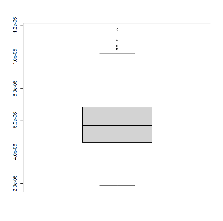
Refer to caption

(a)

Refer to caption

(b)

Figure 2: Comparison of two simulation methods. (a) Boxplot of (5.14) based on 1000 simulations. (b) Path of (5.13) generated by the semi-heuristic (black) and backward (red) Euler methods. Note that both trajectories completely coincide and therefore the black path is not visible on the picture.

5.2.2 Simulation 2: two-sided sandwiched process with equidistant bounds

As the second example, we take

Yt=2.5+0t(1(Yscos(5s))41(3+cos(5s)Ys)4)𝑑s+3BtH,t[0,1],Y_{t}=2.5+\int_{0}^{t}\left(\frac{1}{(Y_{s}-\cos(5s))^{4}}-\frac{1}{(3+\cos(5s)-Y_{s})^{4}}\right)ds+3B^{H}_{t},\quad t\in[0,1], (5.15)

with

ψ(t)φ(t)=3+cos(5t)cos(5t)=3,t[0,1].\psi(t)-\varphi(t)=3+\cos(5t)-\cos(5t)=3,\quad t\in[0,1].

In all simulations, N=100000N=100000, n=20n=20. Simulation of one trajectory takes approximately 0.1601701 seconds. All 1000 generated paths (10 of simulated paths are presented on Fig. 3) stay between the bounds without crossing them.
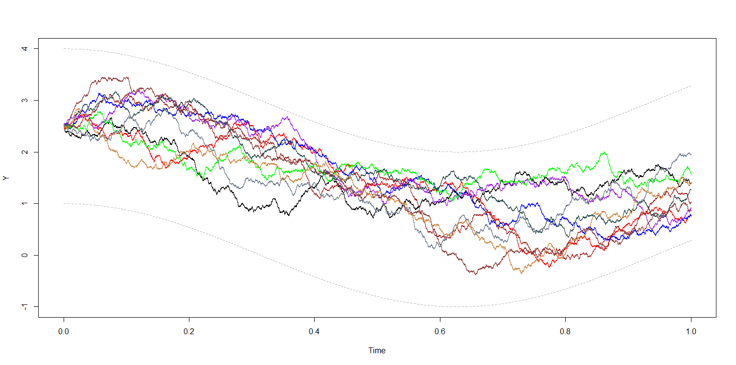
Refer to caption
Figure 3: Ten sample paths of (5.15) generated using the semi-heuristic Euler approximation scheme, N=100000N=100000, n=20n=20.

5.2.3 Simulation 3: two-sided sandwiched process with shrinking bounds

As the final example, we consider

Yt=0t(1(Ys+es)41(esYs)4)𝑑s+BtH,t[0,1],Y_{t}=\int_{0}^{t}\left(\frac{1}{(Y_{s}+e^{-s})^{4}}-\frac{1}{(e^{-s}-Y_{s})^{4}}\right)ds+B^{H}_{t},\quad t\in[0,1], (5.16)

with

ψ(t)φ(t)=2et0,t.\psi(t)-\varphi(t)=2e^{-t}\to 0,\quad t\to\infty.

Once again, N=100000N=100000, n=20n=20. Simulation of one trajectory takes approximately 0.1575801 seconds and all 1000 generated paths (10 of simulated paths are presented on Fig. 4) stay between the bounds without crossing them.
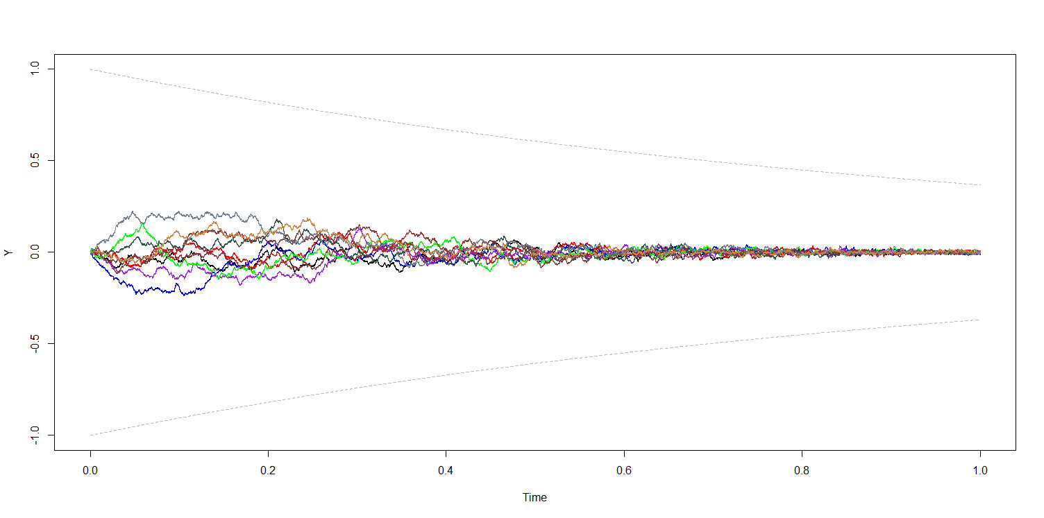
Refer to caption
Figure 4: Ten sample paths of (5.16) generated using the semi-heuristic Euler approximation scheme, N=100000N=100000, n=20n=20.

Acknowledgements

The present research is carried out within the frame and support of the ToppForsk project nr. 274410 of the Research Council of Norway with title STORM: Stochastics for Time-Space Risk Models. The second author is supported by the Ukrainian research project ”Exact formulae, estimates, asymptotic properties and statistical analysis of complex evolutionary systems with many degrees of freedom” (state registration number 0119U100317).

References

  • [1] Alfi, V., Coccetti, F., Petri, A., and Pietronero, L. Roughness and finite size effect in the NYSE stock-price fluctuations. The European physical journal. B 55, 2 (2007), 135–142.
  • [2] Andersen, L. B. G., and Piterbarg, V. V. Moment explosions in stochastic volatility models. Finance and Stochastics 11, 1 (Sept. 2006), 29–50.
  • [3] Anh, V., and Inoue, A. Financial Markets with Memory I: Dynamic Models. Stochastic Analysis and Applications 23, 2 (Jan. 2005), 275–300.
  • [4] Ayache, A., and Peng, Q. Stochastic volatility and multifractional Brownian motion. In Stochastic Differential Equations and Processes (2012), Springer Berlin Heidelberg, p. 211–237.
  • [5] Azmoodeh, E., Sottinen, T., Viitasaari, L., and Yazigi, A. Necessary and sufficient conditions for Hölder continuity of Gaussian processes. Statist. Probab. Lett. 94 (2014), 230–235.
  • [6] Benassi, A., Jaffard, S., and Roux, D. Elliptic Gaussian random processes. Revista Matemática Iberoamericana 13, 1 (1997), 19–90.
  • [7] Beran, J. Statistics for Long-Memory Processes. Chapman and Hall/CRC, 1994.
  • [8] Boguslavskaya, E., Mishura, Y., and Shevchenko, G. Replication of Wiener-transformable stochastic processes with application to financial markets with memory. In Stochastic Processes and Applications (Cham, 2018), S. Silvestrov, A. Malyarenko, and M. Rančić, Eds., Springer International Publishing, pp. 335–361.
  • [9] Bollerslev, T., and Mikkelsen, H. O. Modeling and pricing long memory in stock market volatility. Journal of Econometrics 73, 1 (July 1996), 151–184.
  • [10] Chronopoulou, A., and Viens, F. G. Estimation and pricing under long-memory stochastic volatility. Annals of Finance 8, 2-3 (May 2010), 379–403.
  • [11] Comte, F., Coutin, L., and Renault, E. Affine fractional stochastic volatility models. Annals of Finance 8, 2-3 (July 2010), 337–378.
  • [12] Cox, J. C. The constant elasticity of variance option pricing model. The Journal of Portfolio Management 23, 5 (1996), 15–17.
  • [13] Cox, J. C., Ingersoll, J. E., and Ross, S. A. A re-examination of traditional hypotheses about the term structure of interest rates. The Journal of Finance 36, 4 (Sept. 1981), 769–799.
  • [14] Cox, J. C., Ingersoll, J. E., and Ross, S. A. An intertemporal general equilibrium model of asset prices. Econometrica 53, 2 (Mar. 1985), 363.
  • [15] Cox, J. C., Ingersoll, J. E., and Ross, S. A. A theory of the term structure of interest rates. Econometrica 53, 2 (Mar. 1985), 385.
  • [16] Ding, Z., Granger, C. W., and Engle, R. F. A long memory property of stock market returns and a new model. Journal of Empirical Finance 1, 1 (June 1993), 83–106.
  • [17] Domingo, D., d’Onofrio, A., and Flandoli, F. Properties of bounded stochastic processes employed in biophysics. Stochastic Analysis and Applications 38, 2 (Dec. 2019), 277–306.
  • [18] d’Onofrio, A., Ed. Bounded Noises in Physics, Biology, and Engineering. Springer New York, 2013.
  • [19] Dozzi, M., Kozachenko, Y., Mishura, Y., and Ralchenko, K. Asymptotic growth of trajectories of multifractional Brownian motion, with statistical applications to drift parameter estimation. Stat. Inference Stoch. Process. 21, 1 (2018), 21–52.
  • [20] Friz, P. K., and Hairer, M. A Course on Rough Paths. Springer International Publishing, 2014.
  • [21] Friz, P. K., and Victoir, N. B. Multidimensional Stochastic Processes as Rough Paths: Theory and Applications. Cambridge Studies in Advanced Mathematics. Cambridge University Press, 2010.
  • [22] Garsia, A., Rodemich, E., and Rumsey, H. A real variable lemma and the continuity of paths of some Gaussian processes. Indiana Univ. Math. J. 20 (1970), 565–578.
  • [23] Gatheral, J., Jaisson, T., and Rosenbaum, M. Volatility is rough. Quantitative Finance 18, 6 (Mar. 2018), 933–949.
  • [24] Hong, J., Huang, C., Kamrani, M., and Wang, X. Optimal strong convergence rate of a backward Euler type scheme for the Cox–Ingersoll–Ross model driven by fractional Brownian motion. Stochastic Processes and their Applications 130, 5 (2020), 2675 – 2692.
  • [25] Hu, Y., Nualart, D., and Song, X. A singular stochastic differential equation driven by fractional Brownian motion. Statistics & Probability Letters 78, 14 (2008), 2075 – 2085.
  • [26] Merino, R., Pospíšil, J., Sobotka, T., Sottinen, T., and Vives, J. Decomposition formula for rough Volterra stochastic volatility models. International journal of theoretical and applied finance 24, 02 (2021), 2150008.
  • [27] Mishura, Y., Shevchenko, G., and Shklyar, S. Gaussian processes with Volterra kernels. arXiv:2001.03405 (2020).
  • [28] Mishura, Y., and Yurchenko-Tytarenko, A. Fractional Cox–Ingersoll–Ross process with non-zero “mean”. Modern Stochastics: Theory and Applications 5, 1 (2018), 99–111.
  • [29] Mishura, Y., and Yurchenko-Tytarenko, A. Fractional Cox–Ingersoll–Ross process with small Hurst indices. Modern Stochastics: Theory and Applications 6, 1 (2018), 13–39.
  • [30] Mishura, Y., and Yurchenko-Tytarenko, A. Approximating Expected Value of an Option with Non-Lipschitz Payoff in Fractional Heston-Type Model. International Journal of Theoretical and Applied Finance (June 2020).
  • [31] Mishura, Y., and Yurchenko-Tytarenko, A. Standard and fractional reflected Ornstein-Uhlenbeck processes as the limits of square roots of Cox-Ingersoll-Ross processes. arXiv: 2109.13619 (2021).
  • [32] Nourdin, I. Selected Aspects of Fractional Brownian Motion. Springer Milan, 2012.
  • [33] Nualart, D., and Rascanu, A. Differential equations driven by fractional Brownian motion. Collectanea Mathematica 53, 1 (2002), 55–81.
  • [34] Samorodnitsky, G. Stochastic Processes and Long Range Dependence. Springer International Publishing, 2016.
  • [35] Stoev, S. A., and Taqqu, M. S. How rich is the class of multifractional Brownian motions? Stochastic Process. Appl. 116, 2 (2006), 200–221.
  • [36] Tarasov, V. On history of mathematical economics: Application of fractional calculus. Mathematics 7, 6 (June 2019), 509.
  • [37] Yamasaki, K., Muchnik, L., Havlin, S., Bunde, A., and Stanley, H. E. Scaling and memory in volatility return intervals in financial markets. Proceedings of the National Academy of Sciences 102, 26 (June 2005), 9424–9428.
  • [38] Zhang, S.-Q., and Yuan, C. Stochastic differential equations driven by fractional Brownian motion with locally Lipschitz drift and their implicit Euler approximation. Proceedings of the Royal Society of Edinburgh: Section A Mathematics (2020), 1–27.
  • [39] Zähle, M. Integration with respect to fractal functions and stochastic calculus. i. Probability theory and related fields 111, 3 (1998), 333–374.

Appendix A Appendix: Existence of the local solution

In this Appendix, we give a proof of Theorem 2.2 on the existence of the solution to (0.3) under assumptions (A1)(A3) until the first moment of hitting φ\varphi by the latter. Note that it would be possible to prove this result using a modification of the standard Picard iteration argument, but we choose a different strategy: we approximate the non-Lipschitz drift of (0.3) by a sequence of the Lipschitz ones, obtain a monotonically increasing sequence of processes and prove that their limit is the only solution. Choice of such a method is explained by two points. First, without assumption (A4), the solution may hit φ\varphi and the limiting procedure described in this Appendix allows to see (up to some extent) what happens beyond this moment. Second, the pre-limit processes are very easy to simulate, so they can be used for numerical schemes.

Before going to the proof of Theorem 2.2, we will require several auxiliary results. Let n0>maxt[0,T]|b(t,φ(t)+y)|n_{0}>\max_{t\in[0,T]}|b(t,\varphi(t)+y_{*})|, where yy_{*} is from Assumption (A3). For an arbitrary nn0n\geq n_{0} define the set

𝒢n:={(t,y)𝒟0𝒟y|b(t,y)<n}\begin{gathered}\mathcal{G}_{n}:=\{(t,y)\in\mathcal{D}_{0}\setminus\mathcal{D}_{y_{*}}~|~b(t,y)<n\}\end{gathered}

and consider the functions b~n\tilde{b}_{n}: [0,T]×[0,T]\times\mathbb{R}\to\mathbb{R} of the form

b~n(t,y):={b(t,y),(t,y)𝒢n𝒟y,n,(t,y)[0,T]×(𝒢n𝒟y),\tilde{b}_{n}(t,y):=\begin{cases}b(t,y),&\quad(t,y)\in\mathcal{G}_{n}\cup\mathcal{D}_{y_{*}},\\ n,&\quad(t,y)\in[0,T]\times\mathbb{R}\setminus\left(\mathcal{G}_{n}\cup\mathcal{D}_{y_{*}}\right),\end{cases} (A.1)

bn(t,y):=b~n(t,y)1nb_{n}(t,y):=\tilde{b}_{n}(t,y)-\frac{1}{n}.

Note that each bnb_{n} is Lipschitz continuous, i.e. for all (t,y1),(t,y2)[0,T]×(t,y_{1}),(t,y_{2})\in[0,T]\times\mathbb{R} there exists the constant CC that depends on nn but does not depend on tt such that

|bn(t,y1)bn(t,y2)|C|y1y2|.|b_{n}(t,y_{1})-b_{n}(t,y_{2})|\leq C|y_{1}-y_{2}|.

Using this fact, it is straightforward to prove by the standard fixed point argument that the stochastic differential equation of the form

dYt(n)=bn(t,Yt(n))dt+dZt,Y0(n)=Y0>0,dY^{(n)}_{t}=b_{n}(t,Y^{(n)}_{t})dt+dZ_{t},\quad Y^{(n)}_{0}=Y_{0}>0, (A.2)

has a pathwisely unique solution.

In order to progress, we will require a simple comparison-type result.

Lemma A.1.

Assume that continuous random processes {X1(t),t0}\{X_{1}(t),~t\geq 0\} and {X2(t),t0}\{X_{2}(t),t\geq 0\} satisfy (a.s.) the equations of the form

Xi(t)=X0+0tfi(s,Xi(s))ds+Zt,t0,i=1,2,X_{i}(t)=X_{0}+\int_{0}^{t}f_{i}(s,X_{i}(s))ds+Z_{t},\quad t\geq 0,\quad i=1,2,

where X0X_{0} is a constant and f1f_{1}, f2f_{2}: [0,)×[0,\infty)\times\mathbb{R}\to\mathbb{R} are continuous functions such that for any (t,x)[0,)×(t,x)\in[0,\infty)\times\mathbb{R}:

f1(t,x)<f2(t,x).f_{1}(t,x)<f_{2}(t,x).

Then X1(t)<X2(t)X_{1}(t)<X_{2}(t) a.s. for any t>0t>0.

Proof.

The proof is straightforward. Denote

Δ(t):=X2(t)X1(t)=0t(f2(s,X2(s))f1(s,X1(s)))𝑑s,t0,\Delta(t):=X_{2}(t)-X_{1}(t)=\int_{0}^{t}\left(f_{2}(s,X_{2}(s))-f_{1}(s,X_{1}(s))\right)ds,\quad t\geq 0,

and observe that Δ(0)=0\Delta(0)=0 and that the function Δ\Delta is differentiable with

Δ+(0)=f2(0,X0)f1(0,X0)>0.\Delta^{\prime}_{+}(0)=f_{2}(0,X_{0})-f_{1}(0,X_{0})>0.

It is clear that Δ(t)=Δ+(0)t+o(t)\Delta(t)=\Delta^{\prime}_{+}(0)t+o(t), t0+t\to 0+, whence there exists the maximal interval (0,t)(0,)(0,t^{*})\subset(0,\infty) such that Δ(t)>0\Delta(t)>0 for all t(0,t)t\in(0,t^{*}). It is also clear that

t=sup{t>0|s(0,t):Δ(s)>0}.t^{*}=\sup\{t>0~|~\forall s\in(0,t):\Delta(s)>0\}.

Assume that t<t^{*}<\infty. By the definition of tt^{*} and continuity of Δ\Delta, Δ(t)=0\Delta(t^{*})=0. Hence X1(t)=X2(t)=XX_{1}(t^{*})=X_{2}(t^{*})=X^{*} and

Δ(t)=f2(t,X)f1(t,X)>0.\Delta^{\prime}(t^{*})=f_{2}(t^{*},X^{*})-f_{1}(t^{*},X^{*})>0.

As Δ(t)=Δ(t)(tt)+o(tt)\Delta(t)=\Delta^{\prime}(t^{*})(t-t^{*})+o(t-t^{*}), ttt\to t^{*}, there exists such ε>0\varepsilon>0 that Δ(t)<0\Delta(t)<0 for all t(tε,t)t\in(t^{*}-\varepsilon,t^{*}) which contradicts the definition of tt^{*}. Therefore t=t^{*}=\infty and for all t>0t>0:

X1(t)<X2(t).X_{1}(t)<X_{2}(t).

It is easy to observe that bn(t,y)<bn+1(t,y)b_{n}(t,y)<b_{n+1}(t,y) for any n1n\geq 1 and (t,y)[0,T]×(t,y)\in[0,T]\times\mathbb{R}, whence Yt(n)<Yt(n+1)Y^{(n)}_{t}<Y^{(n+1)}_{t} for all t(0,T]t\in(0,T] and therefore one can define a limit Yt():=limnYt(n)(,]Y^{(\infty)}_{t}:=\lim_{n\to\infty}Y^{(n)}_{t}\in(-\infty,\infty], t[0,T]t\in[0,T].

Proposition A.2.

Let assumptions (A1)(A3) hold. Then, there is a random variable Ψ>maxt[0,T]|φ(t)|\Psi>\max_{t\in[0,T]}|\varphi(t)| such that for any t[0,T]t\in[0,T]:

|Yt()|Ψ<.|Y^{(\infty)}_{t}|\leq\Psi<\infty.
Proof.

Denote η:=Y0φ(0)2\eta:=\frac{Y_{0}-\varphi(0)}{2} and consider

τ1n:\displaystyle\tau^{n}_{1}: =sup{s[0,T]|u[0,s]:Yu(n)φ(u)+η}\displaystyle=\sup\left\{s\in[0,T]~\bigg|~\forall u\in[0,s]:~Y^{(n)}_{u}\geq\varphi(u)+\eta\right\}
=inf{s[0,T]|Ys(n)<φ(s)+η}T.\displaystyle=\inf\left\{s\in[0,T]~\bigg|~Y^{(n)}_{s}<\varphi(s)+\eta\right\}\wedge T.

We shall first prove that for all nn0n\geq n_{0}:

|Yt(n)|\displaystyle|Y^{(n)}_{t}| |Y0|+2maxs[0,T]|Ys(n0)|+5maxs[0,T]|φ(s)|+η\displaystyle\leq|Y_{0}|+2\max_{s\in[0,T]}|Y^{(n_{0})}_{s}|+5\max_{s\in[0,T]}|\varphi(s)|+\eta
+Ct+C0t|Ys(n)|𝑑s+2maxs[0,T]|Zs|,\displaystyle\quad+Ct+C\int_{0}^{t}|Y^{(n)}_{s}|ds+2\max_{s\in[0,T]}|Z_{s}|,

with C>0C>0 being a constant that does not depend on nn. Then the required result follows by Gronwall’s inequality.

For the reader’s convenience, we will divide the proof into several steps to separate cases t[0,τ1n]t\in[0,\tau^{n}_{1}] and t(τ1n,T]t\in(\tau^{n}_{1},T].
Step 1. Fix an arbitrary nn0n\geq n_{0} and assume that t[0,τ1n]t\in[0,\tau^{n}_{1}], i.e. Ys(n)φ(s)+ηY^{(n)}_{s}\geq\varphi(s)+\eta for each sts\leq t. Observe that for all (s,y)𝒟η(s,y)\in\mathcal{D}_{\eta}

|bn(s,y)|C(1+|y|),|b_{n}(s,y)|\leq C(1+|y|), (A.3)

where C>0C>0 is some constant that depends neither on nn nor on ss. Indeed, it is easy to verify using definition of bnb_{n} and assumption (A3) that for all (s,y)𝒟η(s,y)\in\mathcal{D}_{\eta}

|bn(s,y)||bn(s,y)+1n|+1|b(s,y)|+1.|b_{n}(s,y)|\leq\left|b_{n}(s,y)+\frac{1}{n}\right|+1\leq|b(s,y)|+1.

Furthermore, by assumption (A2), for all (s,y)𝒟η(s,y)\in\mathcal{D}_{\eta}

|b(s,y)|\displaystyle|b(s,y)| |b(s,y)b(s,φ(s)+η)|+|b(s,φ(s)+η)|\displaystyle\leq\left|b(s,y)-b\left(s,\varphi(s)+\eta\right)\right|+\left|b\left(s,\varphi(s)+\eta\right)\right|
cη(yφ(s)η)+maxs[0,T]|b(s,φ(s)+η)|\displaystyle\leq c_{\eta}(y-\varphi(s)-\eta)+\max_{s\in[0,T]}\left|b\left(s,\varphi(s)+\eta\right)\right|
(maxs[0,T]|b(s,φ(s)+η)|+cηmaxs[0,T]|φ(s)|+cη(η+1))(1+|y|).\displaystyle\leq\left(\max_{s\in[0,T]}|b\left(s,\varphi(s)+\eta\right)|+c_{\eta}\max_{s\in[0,T]}|\varphi(s)|+c_{\eta}(\eta+1)\right)(1+|y|).

Using (A.3), for an arbitrary nn0n\geq n_{0}:

|Yt(n)|\displaystyle\left|Y^{(n)}_{t}\right| =|Y0+0tbn(s,Ys(n))ds+Zt|\displaystyle=\left|Y_{0}+\int_{0}^{t}b_{n}(s,Y^{(n)}_{s})ds+Z_{t}\right| (A.4)
|Y0|+0t|bn(s,Ys(n))|ds+|Zt|\displaystyle\leq|Y_{0}|+\int_{0}^{t}|b_{n}(s,Y^{(n)}_{s})|ds+|Z_{t}|
|Y0|+Ct+C0t|Ys(n)|ds+maxs[0,T]|Zs|.\displaystyle\leq|Y_{0}|+Ct+C\int_{0}^{t}|Y^{(n)}_{s}|ds+\max_{s\in[0,T]}|Z_{s}|.

Step 2. Assume t>τ1nt>\tau^{n}_{1}. Consider

τ2n(t):=sup{s(τ1n,t]||Ys(n)φ(s)|<η}.\tau_{2}^{n}(t):=\sup\left\{s\in(\tau^{n}_{1},t]~\bigg|~|Y^{(n)}_{s}-\varphi(s)|<\eta\right\}.

Note that |Yτ2n(t)(n)||φ(τ2n(t))|+ηmaxs[0,T]|φ(s)|+η\left|Y^{(n)}_{{\tau^{n}_{2}(t)}}\right|\leq|\varphi\left(\tau_{2}^{n}(t)\right)|+\eta\leq\max_{s\in[0,T]}|\varphi(s)|+\eta and, therefore,

|Yt(n)|\displaystyle|Y^{(n)}_{t}| =|(Yt(n)Yτ2n(t)(n))+Yτ2n(t)(n)|\displaystyle=\left|\left(Y^{(n)}_{t}-Y^{(n)}_{\tau^{n}_{2}(t)}\right)+Y^{(n)}_{\tau^{n}_{2}(t)}\right|
|Yt(n)Yτ2n(t)(n)|+maxs[0,T]|φ(s)|+η.\displaystyle\leq\left|Y^{(n)}_{t}-Y^{(n)}_{\tau^{n}_{2}(t)}\right|+\max_{s\in[0,T]}|\varphi(s)|+\eta.

If τ2n(t)=t\tau^{n}_{2}(t)=t, then |Yt(n)Yτ2n(t)(n)|=0|Y^{(n)}_{t}-Y^{(n)}_{\tau^{n}_{2}(t)}|=0, so |Yt(n)|<maxs[0,T]|φ(s)|+η|Y^{(n)}_{t}|<\max_{s\in[0,T]}|\varphi(s)|+\eta. Otherwise, if τ2n(t)<t\tau^{n}_{2}(t)<t, then, for any s[τ2n(t),t]s\in[\tau^{n}_{2}(t),t]: |Ys(n)φ(s)|η|Y^{(n)}_{s}-\varphi(s)|\geq\eta which means that either Ys(n)φ(s)ηY^{(n)}_{s}\leq\varphi(s)-\eta or Ys(n)φ(s)+ηY^{(n)}_{s}\geq\varphi(s)+\eta for all s[τ2n(t),t]s\in[\tau^{n}_{2}(t),t]. In the first case, taking into account the monotonicity of Ys(n)Y^{(n)}_{s} with respect to nn, we have

Ys(n0)φ(s)Ys(n)φ(s)η,Y^{(n_{0})}_{s}-\varphi(s)\leq Y^{(n)}_{s}-\varphi(s)\leq-\eta,

i.e.

η|Ys(n)φ(s)||Ys(n0)φ(s)|,\eta\leq|Y^{(n)}_{s}-\varphi(s)|\leq|Y^{(n_{0})}_{s}-\varphi(s)|,

so

|Yt(n)Yτ2n(t)(n)|\displaystyle|Y^{(n)}_{t}-Y^{(n)}_{\tau^{n}_{2}(t)}| |Yt(n)φ(t)|+|Yτ2n(t)(n)φ(τ2n(t))|+|φ(t)φ(τ2n(t))|\displaystyle\leq|Y^{(n)}_{t}-\varphi(t)|+|Y^{(n)}_{\tau^{n}_{2}(t)}-\varphi({\tau^{n}_{2}(t)})|+|\varphi(t)-\varphi(\tau^{n}_{2}(t))| (A.5)
|Yt(n0)φ(t)|+|Yτ2n(t)(n0)φ(τ2n(t))|+|φ(t)φ(τ2n(t))|\displaystyle\leq|Y^{(n_{0})}_{t}-\varphi(t)|+|Y^{(n_{0})}_{\tau^{n}_{2}(t)}-\varphi({\tau^{n}_{2}(t)})|+|\varphi(t)-\varphi(\tau^{n}_{2}(t))|
2maxs[0,T]|Yt(n0)|+4maxs[0,T]|φ(s)|.\displaystyle\leq 2\max_{s\in[0,T]}|Y^{(n_{0})}_{t}|+4\max_{s\in[0,T]}|\varphi(s)|.

In the second case, since (s,Ys(n))𝒟η(s,Y^{(n)}_{s})\in\mathcal{D}_{\eta}, we can use (A.3) to obtain that

|Yt(n)Yτ2n(t)(n)|\displaystyle|Y^{(n)}_{t}-Y^{(n)}_{\tau^{n}_{2}(t)}| =|τ2n(t)tb(s,Ys(n))𝑑s+(ZtZτ2n(t))|\displaystyle=\bigg|\int_{\tau^{n}_{2}(t)}^{t}b(s,Y^{(n)}_{s})ds+(Z_{t}-Z_{\tau^{n}_{2}(t)})\bigg|
C(tτ2n(t))+Cτ2n(t)t|Ys(n)|ds+2maxs[0,T]|Zs|\displaystyle\leq C(t-\tau^{n}_{2}(t))+C\int_{\tau^{n}_{2}(t)}^{t}|Y^{(n)}_{s}|ds+2\max_{s\in[0,T]}|Z_{s}|
Ct+C0t|Ys(n)|ds+2maxs[0,T]|Zs|.\displaystyle\leq Ct+C\int_{0}^{t}|Y^{(n)}_{s}|ds+2\max_{s\in[0,T]}|Z_{s}|.

In any situation, for all t>τ1nt>\tau^{n}_{1}:

|Yt(n)|\displaystyle|Y^{(n)}_{t}| 2maxs[0,T]|Ys(n0)|+5maxs[0,T]|φ(s)|+η\displaystyle\leq 2\max_{s\in[0,T]}|Y^{(n_{0})}_{s}|+5\max_{s\in[0,T]}|\varphi(s)|+\eta (A.6)
+Ct+C0t|Ys(n)|ds+2maxs[0,T]|Zs|.\displaystyle+Ct+C\int_{0}^{t}|Y^{(n)}_{s}|ds+2\max_{s\in[0,T]}|Z_{s}|.

Step 3. Taking into account (A.4) and (A.6), it is easy to see that for all t0t\geq 0:

|Yt(n)|\displaystyle|Y^{(n)}_{t}| |Y0|+2maxs[0,T]|Ys(n0)|+5maxs[0,T]|φ(s)|+η\displaystyle\leq|Y_{0}|+2\max_{s\in[0,T]}|Y^{(n_{0})}_{s}|+5\max_{s\in[0,T]}|\varphi(s)|+\eta
+Ct+C0t|Ys(n)|𝑑s+2maxs[0,T]|Zs|,\displaystyle\quad+Ct+C\int_{0}^{t}|Y^{(n)}_{s}|ds+2\max_{s\in[0,T]}|Z_{s}|,

so, by Gronwall’s inequality, for all n1n\geq 1:

|Yt(n)|\displaystyle|Y^{(n)}_{t}| Ψ<,\displaystyle\leq\Psi<\infty, (A.7)

where

Ψ:=(|Y0|+2maxs[0,T]|Ys(n0)|+5maxs[0,T]|φ(s)|+η+CT+2maxs[0,T]|Zs|)eCT.\Psi:=\left(|Y_{0}|+2\max_{s\in[0,T]}|Y^{(n_{0})}_{s}|+5\max_{s\in[0,T]}|\varphi(s)|+\eta+CT+2\max_{s\in[0,T]}|Z_{s}|\right)e^{CT}.

Since the right-hand side of (A.7) does not depend on nn, the claim of the proposition holds for Y()Y^{(\infty)}. ∎

Proposition A.3.

For all t[0,T]t\in[0,T]: Yt()φ(t)Y^{(\infty)}_{t}\geq\varphi(t).

Proof.

Step 1. Fix an arbitrary t[0,T]t\in[0,T] and denote

bn+(s,y):=bn(s,y)0,bn(s,y):=(bn(s,y)0),b_{n}^{+}(s,y):=b_{n}(s,y)\vee 0,\qquad b_{n}^{-}(s,y):=-(b_{n}(s,y)\wedge 0),

bn(s,y)=bn+(s,y)bn(s,y)b_{n}(s,y)=b_{n}^{+}(s,y)-b_{n}^{-}(s,y).
Observe that, by assumption (A3), bn(s,y)=0b_{n}^{-}(s,y)=0 for all (s,y)𝒟0𝒟y(s,y)\in\mathcal{D}_{0}\setminus\mathcal{D}_{y_{*}}, and, by assumption (A2), bnb_{n}^{-} is globally Lipschitz continuous. From Proposition A.2 we obtain that, for some constant L>0L>0 that does not depend on nn and for all s[0,t]s\in[0,t]:

|bn(s,Ys(n))|\displaystyle|b_{n}^{-}(s,Y^{(n)}_{s})| L(1+|Ys(n)|)L(1+Ψ)=:Ψ~,\displaystyle\leq L(1+|Y^{(n)}_{s}|)\leq L(1+\Psi)=:\widetilde{\Psi},

where Ψ~\widetilde{\Psi} is a finite random variable. Hence, since bn(s,Ys(n))b(s,Ys())b^{-}_{n}(s,Y^{(n)}_{s})\to b^{-}(s,Y^{(\infty)}_{s}) pointwise as nn\to\infty, by the dominated convergence theorem,

0tbn(s,Ys(n))𝑑s0tb(s,Ys())𝑑s,n.\int_{0}^{t}b^{-}_{n}(s,Y^{(n)}_{s})ds\to\int_{0}^{t}b^{-}(s,Y^{(\infty)}_{s})ds,\quad n\to\infty.

Taking into account the convergence above and Proposition A.2, the left hand side of

Yt(n)Y0Zt+0tbn(s,Ys(n))𝑑s=0tbn+(s,Ys(n))𝑑sY^{(n)}_{t}-Y_{0}-Z_{t}+\int_{0}^{t}b^{-}_{n}(s,Y^{(n)}_{s})ds=\int_{0}^{t}b^{+}_{n}(s,Y^{(n)}_{s})ds

converges to a finite value as nn\to\infty for each t[0,T]t\in[0,T]. Therefore there exists the limit

limn0tbn+(s,Ys(n))𝑑s<.\lim_{n\to\infty}\int_{0}^{t}b^{+}_{n}(s,Y^{(n)}_{s})ds<\infty. (A.8)

Step 2. Let us now prove that

μ{s[0,T]|Ys(n)φ(s)}0,n,\mu\{s\in[0,T]~|~Y^{(n)}_{s}\leq\varphi(s)\}\to 0,\quad n\to\infty,

with μ\mu being the Lebesgue measure on [0,T][0,T]. Assume that it is not true. i.e. there exist ϵ>0\epsilon>0 and a subsequence {nk:k1}\{n_{k}:~k\geq 1\} such that for all k1k\geq 1:

μ{s[0,T]|Ys(nk)φ(s)}ϵ>0.\mu\{s\in[0,T]~|~Y^{(n_{k})}_{s}\leq\varphi(s)\}\geq\epsilon>0.

In this case,

0Tbnk+(s,Ys(nk))𝑑s\displaystyle\int_{0}^{T}b^{+}_{n_{k}}(s,Y^{(n_{k})}_{s})ds ={s[0,T]|Ys(nk)>φ(s)}bnk+(s,Ys(nk))𝑑s\displaystyle=\int_{\{s\in[0,T]~|~Y^{(n_{k})}_{s}>\varphi(s)\}}b^{+}_{n_{k}}(s,Y^{(n_{k})}_{s})ds
+{s[0,T]|Ys(nk)φ(s)}bnk+(s,Ys(nk))ds\displaystyle\quad+\int_{\{s\in[0,T]~|~Y^{(n_{k})}_{s}\leq\varphi(s)\}}b^{+}_{n_{k}}(s,Y^{(n_{k})}_{s})ds
{s[0,T]|Ys(nk)φ(s)}bnk+(s,Ys(nk))𝑑s\displaystyle\geq\int_{\{s\in[0,T]~|~Y^{(n_{k})}_{s}\leq\varphi(s)\}}b^{+}_{n_{k}}(s,Y^{(n_{k})}_{s})ds
={s[0,T]|Ys(nk)φ(s)}(nk1nk)𝑑s\displaystyle=\int_{\{s\in[0,T]~|~Y^{(n_{k})}_{s}\leq\varphi(s)\}}\left(n_{k}-\frac{1}{n_{k}}\right)ds
nkϵϵnk,k,\displaystyle\geq n_{k}\epsilon-\frac{\epsilon}{n_{k}}\to\infty,\quad k\to\infty,

that contradicts (A.8).
This implies that μ{s[0,T]|Ys()φ(s)}=0\mu\{s\in[0,T]~|~Y^{(\infty)}_{s}\leq\varphi(s)\}=0, i.e. Y()Y^{(\infty)} exceeds φ\varphi a.e. on [0,T][0,T].
Step 3. Assume that there is such τ(0,T]\tau\in(0,T] that Yτ()<φ(τ)Y^{(\infty)}_{\tau}<\varphi(\tau). Then, for all n1n\geq 1:

Yτ(n)<Yτ()φ(τ).Y^{(n)}_{\tau}<Y^{(\infty)}_{\tau}\leq\varphi(\tau).

Fix an arbitrary nn0n\geq n_{0} and denote

τn:=sup{t[0,τ)|Yt(n)>φ(t)}.\begin{gathered}\tau_{-}^{n}:=\sup\{t\in[0,\tau)~|~Y^{(n)}_{t}>\varphi(t)\}.\end{gathered}

Note that, due to continuity of Y(n)Y^{(n)} and Step 2, 0<τn<τT0<\tau_{-}^{n}<\tau\leq T. Furthermore, Yτn(n)φ(τn)=0Y^{(n)}_{\tau_{-}^{n}}-\varphi(\tau_{-}^{n})=0 and for all t(τn,τ]t\in(\tau_{-}^{n},\tau]: Yt(n)φ(t)Y^{(n)}_{t}\leq\varphi(t). Next, for an arbitrary t(τn,τ)t\in(\tau_{-}^{n},\tau):

φ(t)\displaystyle\varphi(t)\geq Yt(n)=Yt(n)Yτn(n)+φ(τn)\displaystyle Y^{(n)}_{t}=Y^{(n)}_{t}-Y^{(n)}_{\tau_{-}^{n}}+\varphi(\tau_{-}^{n})
=\displaystyle= φ(τn)+τntbn(s,Ys(n))𝑑s+(ZtZτn)\displaystyle\varphi(\tau_{-}^{n})+\int_{\tau_{-}^{n}}^{t}b_{n}(s,Y^{(n)}_{s})ds+(Z_{t}-Z_{\tau_{-}^{n}})
=\displaystyle= φ(τn)+(n1n)(tτn)+(ZtZτn)\displaystyle\varphi(\tau_{-}^{n})+\left(n-\frac{1}{n}\right)(t-\tau_{-}^{n})+(Z_{t}-Z_{\tau_{-}^{n}})
\displaystyle\geq φ(τn)+(n1n)(tτn)Λ(tτn)λ,\displaystyle\varphi(\tau_{-}^{n})+\left(n-\frac{1}{n}\right)(t-\tau_{-}^{n})-\Lambda(t-\tau_{-}^{n})^{\lambda},

therefore, for any nn0n\geq n_{0}:

0>Yτ()φ(τ)>Yτ(n)φ(τ)φ(τn)φ(τ)+mint[τn,τ]F(n)(t),0>Y^{(\infty)}_{\tau}-\varphi(\tau)>Y^{(n)}_{\tau}-\varphi(\tau)\geq\varphi(\tau_{-}^{n})-\varphi(\tau)+\min_{t\in[\tau_{-}^{n},\tau]}F^{(n)}(t), (A.9)

with F(n)(t):=(n1n)(tτn)Λ(tτn)λF^{(n)}(t):=\left(n-\frac{1}{n}\right)(t-\tau_{-}^{n})-\Lambda(t-\tau_{-}^{n})^{\lambda}. However, mint[τn,τ]F(n)(t)0\min_{t\in[\tau_{-}^{n},\tau]}F^{(n)}(t)\to 0, nn\to\infty. Indeed,

mint[0,)F(n)(t)mint[τn,τ]F(n)(t)0\min_{t\in[0,\infty)}F^{(n)}(t)\leq\min_{t\in[\tau_{-}^{n},\tau]}F^{(n)}(t)\leq 0

and it is straightforward to verify that F(n)(t)F^{(n)}(t) takes its minimal value on [0,)[0,\infty) at

t:=τn+(λΛn1n)11λt_{*}:=\tau_{-}^{n}+\left(\frac{\lambda\Lambda}{n-\frac{1}{n}}\right)^{\frac{1}{1-\lambda}}

with

F(n)(t)=Λ11λ(λ11λλλ1λ)(n1n)λ1λ0,n.F^{(n)}(t_{*})=\frac{\Lambda^{\frac{1}{1-\lambda}}(\lambda^{\frac{1}{1-\lambda}}-\lambda^{\frac{\lambda}{1-\lambda}})}{\left(n-\frac{1}{n}\right)^{\frac{\lambda}{1-\lambda}}}\to 0,\quad n\to\infty.

Furthermore, it is easy to see from Step 2 that τnτ\tau^{n}_{-}\to\tau, nn\to\infty, so φ(τn)φ(τ)0\varphi(\tau_{-}^{n})-\varphi(\tau)\to 0, nn\to\infty, and therefore (A.9) cannot hold for all nn. The obtained contradiction finalizes the proof. ∎

For arbitrary positive ε<mint[0,T](Ψφ(t))\varepsilon<\min_{t\in[0,T]}\left(\Psi-\varphi(t)\right) and 0t1<t2T0\leq t_{1}<t_{2}\leq T denote

𝒟~ε[t1,t2]:={(t,y)|t[t1,t2],y[φ(t)+ε,Ψ]},\tilde{\mathcal{D}}^{[t_{1},t_{2}]}_{\varepsilon}:=\{(t,y)~|~t\in[t_{1},t_{2}],y\in[\varphi(t)+\varepsilon,\Psi]\},

where Ψ\Psi is from Proposition A.2, and observe that 𝒟~ε[t1,t2]\tilde{\mathcal{D}}^{[t_{1},t_{2}]}_{\varepsilon} is a compact set and bb is continuous on it. Consider also

τ0:=sup{t[0,T]|s[0,t):Ys()>φ(s)}.\tau_{0}:=\sup\{t\in[0,T]~|~\forall s\in[0,t):~Y^{(\infty)}_{s}>\varphi(s)\}.

It is clear that τ0>0\tau_{0}>0 because Y()Y^{(\infty)} is bounded from below by continuous processes Y(n)Y^{(n)} which start from the level Y0>φ(0)Y_{0}>\varphi(0).

Proposition A.4.
  1. 1.

    Y()Y^{(\infty)} is continuous at any tt such that Yt()>φ(t)Y^{(\infty)}_{t}>\varphi(t).

  2. 2.

    For any t<τ0t<\tau_{0}:

    Yt()=Y0+0tb(s,Ys())𝑑s+Zt.Y^{(\infty)}_{t}=Y_{0}+\int_{0}^{t}b(s,Y^{(\infty)}_{s})ds+Z_{t}.
  3. 3.

    Yτ0()=φ(τ0)Y^{(\infty)}_{\tau_{0}}=\varphi(\tau_{0}) and, furthermore, Y()Y^{(\infty)} is left continuous at τ0\tau_{0}:

    limtτ0Yt()=φ(τ0).\lim_{t\to\tau_{0}-}Y^{(\infty)}_{t}=\varphi(\tau_{0}).
Proof.

1. Let t[0,T]t\in[0,T] be such that Yt()>φ(t)Y^{(\infty)}_{t}>\varphi(t). Then there exists n1n0n_{1}\geq n_{0} such that for all nn1n\geq n_{1}: Yt(n)>φ(t)Y^{(n)}_{t}>\varphi(t). Furthermore, because of monotonicity with respect to nn and continuity of both Y(n)Y^{(n)}_{\cdot} and φ\varphi, there is such ε1=ε1(n1)\varepsilon_{1}=\varepsilon_{1}(n_{1}) that for any s[tε1,t+ε1]s\in[t-\varepsilon_{1},t+\varepsilon_{1}]: Ys(n)>φ(s)Y^{(n)}_{s}>\varphi(s), nn1n\geq n_{1}. Furthermore, since for all s[tε1,t+ε1]s\in[t-\varepsilon_{1},t+\varepsilon_{1}] and nn0n\geq n_{0}: Ys(n)<ΨY^{(n)}_{s}<\Psi, for all nn1n\geq n_{1}:

(s,Ys(n))𝒟~ε0[tε1,t+ε1],\left(s,Y^{(n)}_{s}\right)\in\tilde{\mathcal{D}}^{[t-\varepsilon_{1},t+\varepsilon_{1}]}_{\varepsilon_{0}},

with ε0:=minr[tε1,t+ε1](Yr(n1)φ(r))>0\varepsilon_{0}:=\min_{r\in[t-\varepsilon_{1},t+\varepsilon_{1}]}\left(Y^{(n_{1})}_{r}-\varphi(r)\right)>0. Therefore, if n2n1n_{2}\geq n_{1} is such that

n2>max(s,y)𝒟~ε0[tε1,t+ε1]b(s,y),n_{2}>\max_{(s,y)\in\tilde{\mathcal{D}}^{[t-\varepsilon_{1},t+\varepsilon_{1}]}_{\varepsilon_{0}}}b(s,y),

for any nn2n\geq n_{2} and s[tε1,t+ε1]s\in[t-\varepsilon_{1},t+\varepsilon_{1}]: bn(s,Ys(n))=b(s,Ys(n))1nb_{n}(s,Y^{(n)}_{s})=b(s,Y^{(n)}_{s})-\frac{1}{n}, whence

Ys(n)\displaystyle Y^{(n)}_{s} =Ytε1(n)+tε1sbn(r,Yr(n))𝑑r+ZsZtε1\displaystyle=Y^{(n)}_{t-\varepsilon_{1}}+\int_{t-\varepsilon_{1}}^{s}b_{n}(r,Y^{(n)}_{r})dr+Z_{s}-Z_{t-\varepsilon_{1}} (A.10)
=Ytε1(n)+tε1sb(r,Yr(n))drst+ε1n+ZsZtε1.\displaystyle=Y^{(n)}_{t-\varepsilon_{1}}+\int_{t-\varepsilon_{1}}^{s}b(r,Y^{(n)}_{r})dr-\frac{s-t+\varepsilon_{1}}{n}+Z_{s}-Z_{t-\varepsilon_{1}}.

From the choice of n2n_{2}, for any nn2n\geq n_{2} and u[tε1,s]u\in[t-\varepsilon_{1},s]: (u,Yu(n))𝒟ε0(u,Y^{(n)}_{u})\in\mathcal{D}_{\varepsilon_{0}}, therefore, by assumption (A2) and Proposition A.2, there exists a constant L>0L>0 that does not depend on nn such that for any u[tε1,s][tε1,t+ε1]u\in[t-\varepsilon_{1},s]\subset[t-\varepsilon_{1},t+\varepsilon_{1}]

|b(u,Yu(n))|L(1+|Yu(n)|)L(1+Ψ)<,|b(u,Y^{(n)}_{u})|\leq L(1+|Y^{(n)}_{u}|)\leq L(1+\Psi)<\infty,

therefore, by dominated convergence,

limntε1sb(r,Yr(n))𝑑r=tε1sb(r,Yr())𝑑r\lim_{n\to\infty}\int_{t-\varepsilon_{1}}^{s}b(r,Y^{(n)}_{r})dr=\int_{t-\varepsilon_{1}}^{s}b(r,Y^{(\infty)}_{r})dr

which, together with (A.10), implies

Ys()=Ytε1()+tε1sb(r,Yr())𝑑r+ZsZtε1,s[tε1,t+ε1].Y^{(\infty)}_{s}=Y^{(\infty)}_{t-\varepsilon_{1}}+\int_{t-\varepsilon_{1}}^{s}b(r,Y^{(\infty)}_{r})dr+Z_{s}-Z_{t-\varepsilon_{1}},\quad s\in[t-\varepsilon_{1},t+\varepsilon_{1}].

Hence Y()Y^{(\infty)} is continuous on [tε1,t+ε1][t-\varepsilon_{1},t+\varepsilon_{1}] and, in particular, at point tt.
2. Since Y()Y^{(\infty)} is greater than φ\varphi on an arbitrary interval [0,t][0,τ0)[0,t]\subset[0,\tau_{0}), it is continuous on this interval. Therefore, by Dini’s theorem, Y(n)Y^{(n)} converges uniformly to Y()Y^{(\infty)}, nn\to\infty, on [0,t][0,t]. Let n3n_{3} be such that for all nn3n\geq n_{3}: Ys(n)φ(s)>minr[0,t](Yr()φ(r))2=:εY^{(n)}_{s}-\varphi(s)>\frac{\min_{r\in[0,t]}(Y^{(\infty)}_{r}-\varphi(r))}{2}=:\varepsilon_{\infty}, s[0,t]s\in[0,t]. For any s[0,t]s\in[0,t] and nn3n\geq n_{3} it holds that

(s,Ys(n))𝒟~ε[0,t],(s,Y^{(n)}_{s})\in\tilde{\mathcal{D}}^{[0,t]}_{\varepsilon_{\infty}},

so, if n4n3n_{4}\geq n_{3} is such that n4>max(s,y)𝒟~ε[0,t]b(s,y)n_{4}>\max_{(s,y)\in\tilde{\mathcal{D}}^{[0,t]}_{\varepsilon_{\infty}}}b(s,y), for any s[0,t]s\in[0,t] and nn4n\geq n_{4}: bn(s,Ys(n))=b(s,Ys(n))1nb_{n}(s,Y^{(n)}_{s})=b(s,Y^{(n)}_{s})-\frac{1}{n}. Taking into account that

(s,Ys(n)),(s,Ys())𝒟ε(s,Y^{(n)}_{s}),(s,Y^{(\infty)}_{s})\in\mathcal{D}_{\varepsilon}

for any s[0,t]s\in[0,t] with ε(0,ε)\varepsilon\in(0,\varepsilon_{\infty}), we have that, by assumption (A2), there exists a constant cεc_{\varepsilon} that does not depend on nn such that

|bn(s,Ys(n))b(s,Ys())|cε|Ys(n)Ys()|+1n,s[0,t],|b_{n}(s,Y^{(n)}_{s})-b(s,Y^{(\infty)}_{s})|\leq c_{\varepsilon}|Y^{(n)}_{s}-Y^{(\infty)}_{s}|+\frac{1}{n},\quad s\in[0,t],

whence bn(s,Ys(n))b(s,Ys())b_{n}(s,Y^{(n)}_{s})\rightrightarrows b(s,Y^{(\infty)}_{s}) on [0,t][0,t], nn\to\infty. Now the claim can be verified by transition to the limit under the integral.
3. First, note that Yτ0()=φ(τ0)Y^{(\infty)}_{\tau_{0}}=\varphi(\tau_{0}). Indeed, by Proposition A.3, Yt()φ(t)Y^{(\infty)}_{t}\geq\varphi(t) for all t[0,T]t\in[0,T] and, if Yτ0()>φ(τ0)Y^{(\infty)}_{\tau_{0}}>\varphi(\tau_{0}), then Y()Y^{(\infty)} is continuous at τ0\tau_{0} and therefore exceeds φ\varphi on some interval [τ0,τ0+δ)[\tau_{0},\tau_{0}+\delta), that contradicts the definition of τ0\tau_{0}. Now it is sufficient to verify that

lim suptτ0Yt()=φ(τ0).\limsup_{t\to\tau_{0}-}Y^{(\infty)}_{t}=\varphi(\tau_{0}).

Assume it is not true and there is such x(0,)x\in(0,\infty) that

lim suptτ0Yt()=φ(τ0)+x.\limsup_{t\to\tau_{0}-}Y^{(\infty)}_{t}=\varphi(\tau_{0})+x.

Note also that x<x<\infty since, by Proposition A.2, Y()Y^{(\infty)} is bounded from above by the (random) constant Ψ\Psi.
Let δx\delta_{x} be such that for any t[τ0δx,τ0]t\in[\tau_{0}-\delta_{x},\tau_{0}]: |φ(t)φ(τ0)|<x4|\varphi(t)-\varphi(\tau_{0})|<\frac{x}{4}. Denote

OPENεx:=mint[τ0δ,τ0](φ(τ0)+x4φ(t)))\varepsilon_{x}:=\min_{t\in[\tau_{0}-\delta,\tau_{0}]}\left(\varphi(\tau_{0})+\frac{x}{4}-\varphi(t))\right)

and observe that εx>0\varepsilon_{x}>0 and φ(t)+εxφ(τ0)+x4\varphi(t)+\varepsilon_{x}\leq\varphi(\tau_{0})+\frac{x}{4} whenever t[τ0δ,τ0]t\in[\tau_{0}-\delta,\tau_{0}].
If x>0x>0, for any δ(0,δx)\delta\in(0,\delta_{x}) there is such tδ(τ0δ,τ0)t_{\delta}\in(\tau_{0}-\delta,\tau_{0}) that Ytδ()φ(τ0)+3x4Y^{(\infty)}_{t_{\delta}}\geq\varphi(\tau_{0})+\frac{3x}{4}. Let such δ(0,δx)\delta\in(0,\delta_{x}) and tδt_{\delta} be fixed. Since Ytδ(n)Ytδ()Y^{(n)}_{t_{\delta}}\uparrow Y^{(\infty)}_{t_{\delta}}, n1n\geq 1, there is such nδn_{\delta} that for all nnδn\geq n_{\delta}:

Ytδ(n)φ(τ0)+x2.Y^{(n)}_{t_{\delta}}\geq\varphi(\tau_{0})+\frac{x}{2}.

It is clear that Yτ0(n)<φ(τ0)Y^{(n)}_{\tau_{0}}<\varphi(\tau_{0}) therefore, for nnδn\geq n_{\delta} one can consider the moment

θn:=inf{t(tδ,τ0)|Yt(n)=φ(τ0)+x4}.\theta^{n}:=\inf\left\{t\in(t_{\delta},\tau_{0})~|~Y^{(n)}_{t}=\varphi(\tau_{0})+\frac{x}{4}\right\}.

From the continuity of Y(n)Y^{(n)}, Yθn(n)=φ(τ0)+x4Y^{(n)}_{\theta^{n}}=\varphi(\tau_{0})+\frac{x}{4}, so Yθn(n)Ytδ(n)<x4Y^{(n)}_{\theta^{n}}-Y^{(n)}_{t_{\delta}}<-\frac{x}{4}. On the other hand, from definition of θn\theta^{n} and Proposition A.2, for all t[tδ,θn]t\in[t_{\delta},\theta^{n}]:

(t,Yt(n))[tδ,θxn]×[φ(τ0)+x4,Ψ]𝒟~εx[τ0δx,τ0].(t,Y^{(n)}_{t})\in[t_{\delta},\theta^{n}_{x}]\times\left[\varphi(\tau_{0})+\frac{x}{4},\Psi\right]\subset\tilde{\mathcal{D}}^{[\tau_{0}-\delta_{x},\tau_{0}]}_{\varepsilon_{x}}.

Let n~δ>nδ\tilde{n}_{\delta}>n_{\delta} be such that

n~δ>max(s,y)𝒟~εx[τ0δx,τ0]b(s,y).\tilde{n}_{\delta}>\max_{(s,y)\in\tilde{\mathcal{D}}^{[\tau_{0}-\delta_{x},\tau_{0}]}_{\varepsilon_{x}}}b(s,y).

For any t[tδ,θx]t\in[t_{\delta},\theta_{x}] and nn~δn\geq\tilde{n}_{\delta}:

bn(t,Yt(n))=b(t,Yt(n))1nb_{n}(t,Y^{(n)}_{t})=b(t,Y^{(n)}_{t})-\frac{1}{n}

and, therefore, we obtain that

x4\displaystyle-\frac{x}{4} >Yθn(n)Ytδ(n)=tδθnbn(s,Ys(n))𝑑s+(ZθnZtδ)\displaystyle>Y^{(n)}_{\theta^{n}}-Y^{(n)}_{t_{\delta}}=\int_{t_{\delta}}^{\theta^{n}}b_{n}(s,Y^{(n)}_{s})ds+(Z_{\theta^{n}}-Z_{t_{\delta}})
=tδθnb(s,Ys(n))𝑑s1n(θntδ)+(ZθnZtδ)\displaystyle=\int_{t_{\delta}}^{\theta^{n}}b(s,Y^{(n)}_{s})ds-\frac{1}{n}(\theta^{n}-t_{\delta})+(Z_{\theta^{n}}-Z_{t_{\delta}})
=tδθnb+(s,Ys(n))𝑑stδθnb(s,Ys(n))𝑑s1n(θntδ)+(ZθnZtδ)\displaystyle=\int_{t_{\delta}}^{\theta^{n}}b^{+}(s,Y^{(n)}_{s})ds-\int_{t_{\delta}}^{\theta^{n}}b^{-}(s,Y^{(n)}_{s})ds-\frac{1}{n}(\theta^{n}-t_{\delta})+(Z_{\theta^{n}}-Z_{t_{\delta}})
tδθnb(s,Ys(n))ds1n(θntδ)Λ(θntδ)α\displaystyle\geq-\int_{t_{\delta}}^{\theta^{n}}b^{-}(s,Y^{(n)}_{s})ds-\frac{1}{n}(\theta^{n}-t_{\delta})-\Lambda(\theta^{n}-t_{\delta})^{\alpha}
(max(s,y)𝒟~εx[τ0δx,τ0]b(s,y)+1n)(θxntδ)Λ(θxntδ)λ\displaystyle\geq-\left(\max_{(s,y)\in\tilde{\mathcal{D}}^{[\tau_{0}-\delta_{x},\tau_{0}]}_{\varepsilon_{x}}}b^{-}(s,y)+\frac{1}{n}\right)(\theta^{n}_{x}-t_{\delta})-\Lambda(\theta^{n}_{x}-t_{\delta})^{\lambda}
(maxy𝒟~εx[τ0δx,τ0]b(s,y)+1n)δΛδλ,\displaystyle\geq-\left(\max_{y\in\tilde{\mathcal{D}}^{[\tau_{0}-\delta_{x},\tau_{0}]}_{\varepsilon_{x}}}b^{-}(s,y)+\frac{1}{n}\right)\delta-\Lambda\delta^{\lambda},

i.e. for any δ(0,δx)\delta\in(0,\delta_{x}):

δmaxy𝒟~εx[τ0δx,τ0]b(s,y)+Λδλx4,\delta\max_{y\in\tilde{\mathcal{D}}^{[\tau_{0}-\delta_{x},\tau_{0}]}_{\varepsilon_{x}}}b^{-}(s,y)+\Lambda\delta^{\lambda}\geq\frac{x}{4},

which is not possible. The obtained contradiction implies that x=0x=0, i.e.

lim suptτ0Yt()=φ(τ0).\limsup_{t\to\tau_{0}-}Y^{(\infty)}_{t}=\varphi(\tau_{0}).

Now, let us move to the proof of Theorem 2.2.

Proof of Theorem 2.2.

By Proposition A.4, Y=Y()Y=Y^{(\infty)} indeed satisfies the equation of the required form. Let Y~\tilde{Y} satisfy the equation (0.3) on [0,t][0,τ~0τ0)[0,t]\subset[0,\tilde{\tau}_{0}\wedge\tau_{0}). Then it is continuous on [0,t][0,t] and therefore mins[0,t](Y~sφ(s))>0\min_{s\in[0,t]}(\tilde{Y}_{s}-\varphi(s))>0. Let ε:=mins[0,t](Y~sφ(s))mins[0,t](Ys()φ(s))\varepsilon:=\min_{s\in[0,t]}(\tilde{Y}_{s}-\varphi(s))\wedge\min_{s\in[0,t]}(Y^{(\infty)}_{s}-\varphi(s)) and choose n~\tilde{n} such that for all nn~n\geq\tilde{n}: n>max(s,y)𝒟~ε[0,t]b(s,y)n>\max_{(s,y)\in\tilde{\mathcal{D}}^{[0,t]}_{\varepsilon}}b(s,y). Then b(s,Y~s)=b~n(s,Y~s)b(s,\tilde{Y}_{s})=\tilde{b}_{n}(s,\tilde{Y}_{s}), s[0,t]s\in[0,t], nn~n\geq\tilde{n}, where b~n\tilde{b}_{n} is defined by (A.1), whence

Y~s=Y0+0sb~n(s,Y~u)𝑑u+Zs,s[0,t].\tilde{Y}_{s}=Y_{0}+\int_{0}^{s}\tilde{b}_{n}(s,\tilde{Y}_{u})du+Z_{s},\quad s\in[0,t].

However, Y()Y^{(\infty)} also satisfies the equation above and, since the latter has a unique solution, Y~s=Ys()\tilde{Y}_{s}=Y^{(\infty)}_{s} for all s[0,t]s\in[0,t]. Now it is easy to deduce that τ0=τ~0\tau_{0}=\tilde{\tau}_{0} and Y~t=Yt()=Yt\tilde{Y}_{t}=Y^{(\infty)}_{t}=Y_{t} for all t[0,τ0]t\in[0,\tau_{0}]. ∎