arXiv is now an independent nonprofit! Learn more
License: arXiv.org perpetual non-exclusive license
arXiv:2012.08369v2 [math.SP] 06 Jul 2021

Scattering resonances of large weakly open quantum graphs

Maxime Ingremeau Note: Université Côte d’Azur, Laboratoire J.A. Dieudonné
Abstract

In this paper, we consider a sequence of open quantum graphs, with uniformly bounded data, and we are interested in the asymptotic distribution of their scattering resonances. Supposing that the number of leads in our quantum graphs is small compared to the total number of edges, we show that most resonances are close to the real axis. More precisely, the asymptotic distribution of resonances of our open quantum graphs is the same as the asymptotic distribution of the square-root of the eigenvalues of the closed quantum graphs obtained by removing all the leads.

1 Introduction

1.1 Weyl’s laws for scattering resonances

When dealing with Schrödinger operators in d\mathbb{R}^{d}, with a compactly supported potential, the spectrum of the operator consists of [0,+)[0,+\infty), along with finitely many negative eigenvalues. Thus, a lot of relevant spectral information about such operators consist, not in the spectrum and the eigenfunctions themselves, but rather in the scattering resonances and scattering states. These states are eigenfunctions which are not square-integrable, but instead are outgoing at infinity. The associated eigenvalues are the scattering resonances, which are complex numbers having the following interpretation: the real part is associated to the speed of oscillations, while the imaginary part corresponds to the escape rate of the scattering state towards infinity, when propagated by the wave equation.

For instance, in dimension 1, a number zz\in\mathbb{C} is a resonance of an operator Δ+V-\Delta+V if there exists a function fC()f\in C^{\infty}(\mathbb{R}) such that

{Δf+Vf=z2ff(x)=a±e±izx when ±x>>1.\begin{cases}-\Delta f+Vf=z^{2}f\\ f(x)=a_{\pm}e^{\pm izx}~~\text{ when $\pm x>>1$}.\end{cases}

We refer the reader to the recent monograph [16] both for a friendly introduction to scattering resonances, and for a comprehensive presentation of this field of research.

Scattering resonances can be seen as (square roots of) eigenvalues of a non-selfadjoint operator. It is notorious that the spectrum of non-selfadjoint operators is much more difficult to understand than that of self-adjoint ones; this is mainly due to pseudospectral effects, where a small perturbation in the operator can produce large perturbations of the spectrum.

Thus, it is complicated to determine the localization of the resonances. In dimension d=1d=1, it is possible to count the number of resonances in large disks. Namely, if we denote by N(R)N(R) the number of resonances in D(0,R)D(0,R) counted with multiplicity, we have

N(R)RdR+2Vol(chsupp(V))π,\frac{N(R)}{R^{d}}\underset{R\to+\infty}{\longrightarrow}\frac{2\mathrm{Vol}(\mathrm{chsupp}(V))}{\pi}, (1)

where Vol(chsupp(V))\mathrm{Vol}(\mathrm{chsupp}(V)) denotes the length of the convex hull of the support of VV.

Equation (1) was first proved for some special case of VV in [35], and then generalized in [40] (see also [20] and [37]). It can be seen as an analogue of the classical Weyl’s law for the eigenvalues of the Laplacian in a bounded domain.

In higher dimension, it is not known if the analogue of (1) holds. All that is known in general is the upper bound proven in [41], saying that N(R)CVRdN(R)\leq C_{V}R^{d}.

Another interesting problem is to count the number of resonances not in disks, but in strips below the real axis. From a physical point of view, this is more relevant, as the resonances close to the real axis are related to resonant states which spend a long time in the system, before they escape to infinity. This question is often studied in the context of geometric scattering, or in the semiclassical framework. We refer to [42] for an account of the recent developments in this direction.

1.2 Scattering resonances on quantum graphs

As explained in the previous section, it is easier to count resonances of Schrödinger operators on \mathbb{R} than on d\mathbb{R}^{d}. A popular family of one-dimensional systems is that of quantum graphs. A quantum graph is a graph where each edge is endowed with a length, and each vertex, with a boundary condition. Eigenfunctions on the quantum graph are eigenfunctions of the Laplacian on each edge (and hence, are complex exponentials), satisfying the required boundary conditions at each vertex. The most natural boundary conditions are the Kirchhoff (or Neumann-Kirchhoff) boundary conditions (see Definition 2); in all this paper, we will be working with these conditions.

Though very simple to describe, quantum graphs and their spectrum have been successfully used as a model of quantum chaos since the pioneering work of Kottos and Smilansky [28]. Here, we are interested in quantum graphs where, to some of the vertices, we attach semi-infinite edges (or leads). Scattering resonances on such open quantum graphs are complex numbers zz such that there exists an eigenfunction satisfying the boundary conditions at each vertex, and equal to a constant times eizxe^{izx} on every lead. Resonances can also be seen as poles of the scattering matrix or as poles of the scattering determinant (see [19]).

Counting resonances in disks

It is natural to wonder if (1) holds on open quantum graphs. A natural candidate to replace the constant Vol(chsupp(V))\mathrm{Vol}(\mathrm{chsupp}(V)) would be the length of the (finite part of the) quantum graph, i.e., the sum of the lengths of all the edges that are not leads.

Actually, there are examples where N(R)N(R) behaves asymptotically like a constant times RR, where the constant is not 2π\frac{2}{\pi} times the length of the graph. Such an open quantum graph is sometimes called a non-Weyl graph. In [14], it was shown that, on an open quantum graph with Kirchhoff boundary conditions at every vertex, we have N(R)Rc\frac{N(R)}{R}\longrightarrow c, where cc is 2π\frac{2}{\pi} times the length of the graph if and only if the graph is unbalanced, i.e., at every vertex, the number of internal edges is different from the number of leads.

The simplest example of a non-Weyl (thus, not unbalanced) quantum graph is the following: if we have a vertex to which one internal edge and one lead are attached, the situation is equivalent to the one we obtain by removing the vertex and the lead, and replacing the edge by a lead; this would thus reduce the length of the quantum graph. Other examples of non-Weyl graphs were constructed in [14], [32], [18], [13]. The article [31] provides a nice presentation of all these results.

Counting resonances in strips

Just as for Schrödinger operators on d\mathbb{R}^{d}, it is interesting to count the number of resonances in strips below the real axis, instead of disks. In [14], it is shown that, for quantum graphs satisfying Kirchhoff boundary conditions, the resonances all lie in a strip of the form Imz[K,0]\operatorname{Im}z\in[-K,0]. To our knowledge, no explicit expression has ever been given for KK; we will do so in Lemma 1 below in the case of unbalanced quantum graphs.

It is natural to wonder if we can also have a non-trivial upper bound on the imaginary part of resonances, that is to say, if they do all lie in a strip of the form Imz[K,K]\operatorname{Im}z\in[-K,-K^{\prime}] for some K>0K^{\prime}>0.

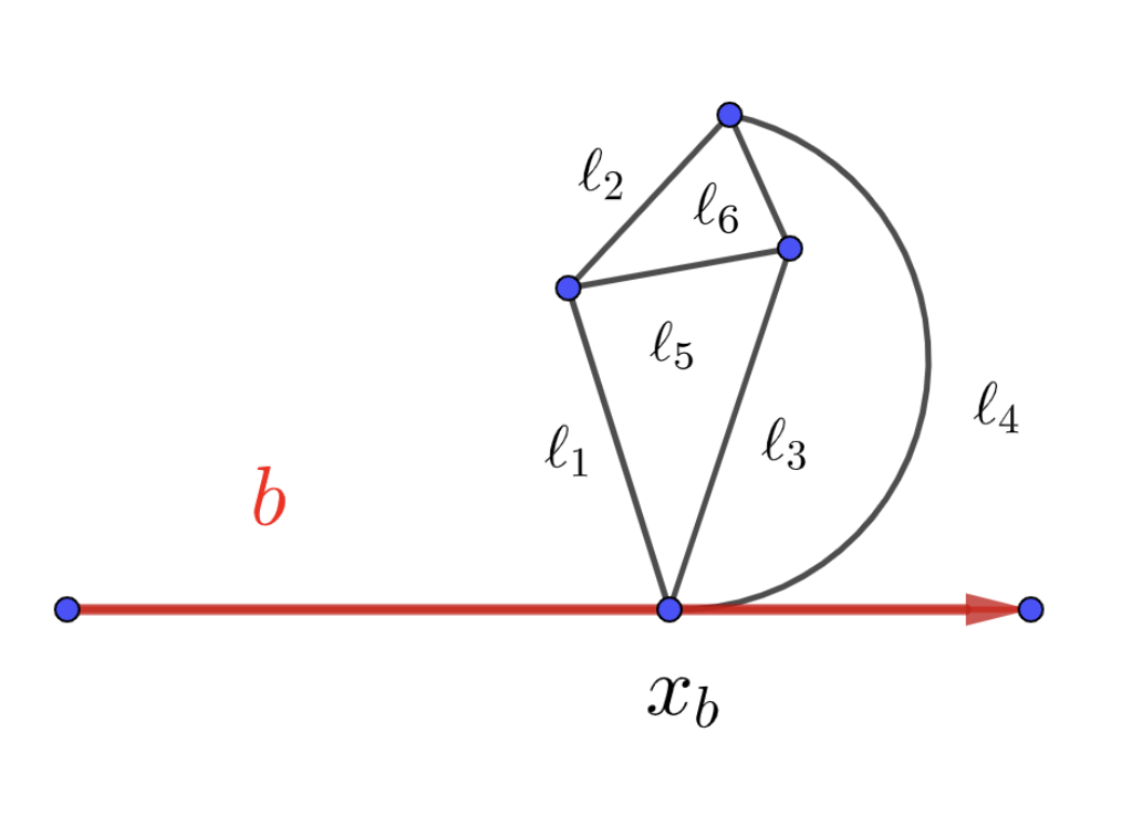
This cannot hold in general, as there can be resonances on the real axis. This is something typical of quantum graphs, related to the fact that, on a quantum graph, there can exist eigenfunctions which vanish on a large part of the graph. For instance, if a quantum graph contains a cycle whose edges have lengths that are all commensurate, it is possible to build eigenfunctions which will vanish on every vertex of the cycle, and on all the edges that are not part of the cycle (see Figure 1 in the appendix). This is in strict opposition to what happens for Schrödinger operators in bounded domains or on manifolds, where the unique continuity principle forbids an eigenfunction to vanish on an open set.

Actually, this situation is highly non-typical: it is shown in [17] and [30] that, if a quantum graph has a resonance on the real axis, then a small perturbation of the lengths will turn it into a resonance with negative imaginary part. Also, it is shown in [12, Theorem 4.2] that, for almost all choices of edge lengths, there are no resonances on the real axis. So far, the only known examples of quantum graphs having resonances on the real axis either have some loop, some vertices of degree 2, or have the lengths of the edges on a cycle all commensurate (see Figure 1 in Appendix A). It is thus natural to think that, when all edge lengths are rationally independent, all degrees are at least 3, and the graph contains no loops, there cannot be any resonance on the real axis. We will show in Appendix A that this is not the case: we show (in a non-constructive way) the existence of quantum graphs containing no loops, having minimal degree larger than 3, and with rationally independent edge lengths, but having some resonances on the real axis.

Coming back to the existence of a resonance gap, i.e., to the question of whether resonances lie in a strip of the form Imz[K,K]\operatorname{Im}z\in[-K,-K^{\prime}] for some K>0K^{\prime}>0, the analogy with semiclassical Schrödinger operators may lead us to look for criteria that are less related to arithmetic of the edge lengths, and more to some classical dynamics. In the physics literature, this was proposed in [4], where the authors introduce some classical dynamics on a quantum graph, introduce a topological pressure11 1 analogue to the topological pressure of half the unstable Jacobian for semiclassical Schrödinger operators whose classical dynamics have a hyperbolic trapped set. See [33] for a definition of this quantity in the case of semiclassical Schrödinger operators., and claim that, if this pressure is negative, there should be a resonance gap.

This statement was disproved in [23] thanks to physical and numerical arguments, and in [12] by mathematical proofs. Indeed, in [12], the authors show that, for quantum graphs that are not trees, and have rationally independent edge lengths, there exist resonances arbitrarily close to the real axis (and with arbitrarily large real parts). The authors are even able to give an interesting lower bound on the number of resonances close to the real axis.

Finally, let us mention that, along with scattering resonances on an open quantum graph, many other non-selfadjoint problems have been considered on quantum graphs, like the damped wave equation, Schrödinger operators with complex potentials, or non-selfadjoint conditions at the vertices. We refer the reader to the introduction of [36] for a presentation of the advances on such topics.

1.3 Resonances of large quantum graphs

In this paper, we will not be interested in the resonances of a single quantum graph. We will rather consider a sequence of open quantum graphs 𝒬N\mathcal{Q}_{N}, having a number of vertices and edges of the order of NN, and will consider the asymptotic distribution of their resonances. Namely the kind of question we will be interested in is the following:

Given a region Ω, what is the asymptotic\displaystyle\text{Given a region $\Omega\subset\mathbb{C}$, what is the asymptotic} (2)
number of resonances of 𝒬N in Ω as N+ ?\displaystyle\text{number of resonances of $\mathcal{Q}_{N}$ in $\Omega$ as $N\longrightarrow+\infty$ ?}

Hence, we consider here the large graph limits instead of the large frequency limits.

To our knowledge, this is the first time in the mathematical literature that resonances of large open quantum graphs are considered. However, for closed quantum graphs (i.e., quantum graphs without leads, which is the situation the most frequently considered), the large graph limits has been a subject of growing interest in the past few years. An important motivation for that was the question of Quantum Ergodicity, which is a property of equidistribution of the eigenfunctions in systems enjoying a chaotic (or just ergodic) classical dynamics. Although quantum graphs are a popular model of quantum chaos, it was shown in [11] that, in general, Quantum Ergodicity does not hold on a given quantum graph. It thus became natural to consider eigenfunctions on a sequence of quantum graphs of increasing size. See for instance [6], [22], [25] [9], [24] and [3] for examples of families of quantum graphs for which quantum ergodicity holds, and [7] for an example where it doesn’t.

Let us also mention [2], where the question (2) is addressed for closed quantum graphs (hence, the resonances are just the square roots of the usual eigenvalues of selfadjoint operators, which are thus on the real axis). Instead of counting exactly the number of resonances in a set Ω\Omega, it is more natural to consider the empirical spectral measures

μ𝒬𝒩:=1(𝒬N)zRes(𝒬N)δz,\mu_{\mathcal{Q_{N}}}:=\frac{1}{\mathcal{L}(\mathcal{Q}_{N})}\sum_{z\in\mathrm{Res}(\mathcal{Q}_{N})}\delta_{z},

where (𝒬N)\mathcal{L}(\mathcal{Q}_{N}) is the sum of the lengths of the edges of 𝒬N\mathcal{Q}_{N}, Res(𝒬N)\mathrm{Res}(\mathcal{Q}_{N}) is the set of resonances of 𝒬N\mathcal{Q}_{N}. It is thus a locally finite measure, which is supported on \mathbb{R} in the case of closed graphs.

Benjamini-Schramm convergence of quantum graphs

In [2], the authors show that a natural criterion to obtain convergence of the empirical spectral measures is to suppose Benjamini-Schramm convergence (also dubbed local weak convergence) of the quantum graphs. For a sequence of discrete graphs (GN)(G_{N}), we say that it converges in the sense of Benjamini-Schramm ([10, 1]) if for any finite rooted graph (F,o)(F,o) and kk\in\mathbb{N}, the fraction of points xGNx\in G_{N} such that BGN(x,k)(F,o)B_{G_{N}}(x,k)\cong(F,o) has a limit, where BGN(x,k)B_{G_{N}}(x,k) is the ball of radius kk around xx in the graph GNG_{N}. The limit is then a probability measure on the set of rooted graphs.

This definition of Benjamini-Schramm convergence for discrete graphs can be extended to the case quantum graphs; we will recall how to do so in section 3.3.1. We will also recall that, if a sequence of quantum graphs has uniformly bounded degrees and edge lengths, we may always extract a subsequence which converges in the sense of Benjamini-Schramm.

The main result of [2] can be summed up as follows: If a sequence of closed quantum graphs (𝒬N)(\mathcal{Q}_{N}) has uniformly bounded degrees and edge lengths, and converges in the sense of Benjamini-Schramm to some probability measure \mathbb{P} on the set of rooted quantum graphs, then μ𝒬N\mu_{\mathcal{Q}_{N}} converges vaguely to some measure depending only on \mathbb{P}. More precisely, for any continuous compactly supported function χCc()\chi\in C_{c}(\mathbb{R}), we have22 2 Note that, in [2], the authors define the empirical spectral measures on closed quantum graphs as sums of Dirac masses on the eigenvalues, which are squares of resonances. This is why the function we integrate in (3) is χ(z)\chi(\sqrt{z}).

1(𝒬N)xRes(𝒬N)χ(x)N+χ(x)dμ(x)=:𝐐χ(H𝒬)(𝐱𝟎,𝐱𝟎)𝑑(𝒬,𝐱𝟎)\frac{1}{\mathcal{L}(\mathcal{Q}_{N})}\sum_{x\in\mathrm{Res}(\mathcal{Q}_{N})}\chi(x)\underset{N\to+\infty}{\longrightarrow}\int_{\mathbb{R}}\chi(\sqrt{x})\mathrm{d}\mu_{\mathbb{P}}(x)=:\int_{\mathbf{Q}_{*}}\chi\big(\sqrt{H_{\mathcal{Q}}}\big)(\mathbf{x_{0}},\mathbf{x_{0}})\mathrm{d}\mathbb{P}(\mathcal{Q},\mathbf{x_{0}}) (3)

where H𝒬H_{\mathcal{Q}} is the Schrödinger operator on the limiting random quantum graph 𝒬\mathcal{Q}, χ(H𝒬)(𝐱𝟎,𝐱𝟎)\chi\big(\sqrt{H_{\mathcal{Q}}}\big)(\mathbf{x_{0}},\mathbf{x_{0}}) is the value of the Schwartz kernel of the operator χ(H𝒬)\chi\big(\sqrt{H_{\mathcal{Q}}}\big) at the root 𝐱𝟎\mathbf{x_{0}} and 𝐐\mathbf{Q}_{*} is a set of (equivalence classes of) rooted quantum graphs.

Presentation of our main result

The main result of this paper is a generalization33 3 Note however, that we only consider case of Kirchhoff boundary conditions here, while more general boundary conditions are treated in [2]. Actually, the proofs of [2] are much simpler when only Kirchhoff boundary conditions are considered. of (3) to the case of a sequence of open quantum graphs converging, in the sense of Benjamini-Schramm, to a probability measure supported on the set of rooted closed quantum graphs:

Let (𝒬N)(\mathcal{Q}_{N}) be a sequence of unbalanced open quantum graphs with NN vertices, having uniformly bounded degree and edge lengths. Suppose that (𝒬N)(\mathcal{Q}_{N}) converges, in the sense of Benjamini-Schramm, to a measure probability \mathbb{P} supported on the set of rooted closed quantum graphs. Then 𝒬N\mathcal{Q}_{N} satisfies (30). In particular, μ𝒬N\mu_{\mathcal{Q}_{N}} converges vaguely to some measure on \mathbb{R} depending only on \mathbb{P}.

Recall that, up to extracting a subsequence, we may always suppose that (𝒬N)(\mathcal{Q}_{N}) converges in the sense of Benjamini-Schramm. The assumption that the limit is on the set of closed quantum graphs is equivalent to supposing that the number of leads is a o(N)o(N).

An informal, but illuminating, formulation of our result is the following. Let 𝒬~N\widetilde{\mathcal{Q}}_{N} be the quantum graph obtained from 𝒬N\mathcal{Q}_{N} by removing all the leads from it. Then, if the number of leads of 𝒬N\mathcal{Q}_{N} is a o(N)o(N), the resonances of 𝒬N\mathcal{Q}_{N} and the square-root of the eigenvalues of 𝒬~N\widetilde{\mathcal{Q}}_{N} are asymptotically distributed the in same way.

In particular, this shows that, if 𝒦\mathcal{K} is a compact set which does not intersect the real axis, then the number of resonances of 𝒬N\mathcal{Q}_{N} in 𝒦\mathcal{K} is a o(N)o(N).

Resonances mildly close to the real axis

In Theorem 4 below, we will show more precise estimates, depending on the number of leads in 𝒬N\mathcal{Q}_{N}. In particular, if the number of leads in 𝒬N\mathcal{Q}_{N} is bounded independently of NN, we show that the number of resonances 𝒬N\mathcal{Q}_{N} in [a,b]+i[,δN][a,b]+i[-\infty,-\delta_{N}] is a O(1δN5/2)O\left(\frac{1}{\delta_{N}^{5/2}}\right). We don’t believe this bound is optimal; it would be very interesting (and probably hard) to describe the asymptotic number of resonances 𝒬N\mathcal{Q}_{N} in [a,b]+i[,δN][a,b]+i[-\infty,-\delta_{N}], for instance when δN\delta_{N} is a negative power of NN. To this end, the numerical computations done in [4, Section 7] could be a good starting point, although their NN isn’t very large, and the asymptotic they consider is not very clear (they seem to consider the asymptotic δN>>1\delta_{N}>>1, although there are no resonances away from a horizontal strip).

Relation to other works

The large quantum graph limit we consider (with few leads) has analogues in the realm of Schrödinger operators. Namely, consider a potential VL()V\in L^{\infty}(\mathbb{R}), spatially extended (for instance, periodic with respect to d\mathbb{Z}^{d}, or a random potential), and write VR(x):=V(x)𝟏|x|RV_{R}(x):=V(x)\mathbf{1}_{|x|\leq R}. It is natural to wonder if the resonances of Δ+VR-\Delta+V_{R} will somehow converge to the real axis, and approach the spectrum of the fully extended operator Δ+V-\Delta+V. The reason why such a phenomenon would happen is that, to escape from the support of the potential and go to infinity, the waves must pass through a spherical layer close to the boundary of the ball. As the ball becomes large, this layer has a volume much smaller than the total volume of the ball. Hence, this situation is very similar to having few leads on a large quantum graph.

To our knowledge, this problem of resonances for potentials with a wide support was first studied in [27] for both periodic and random potentials in \mathbb{Z}, which are truncated outside of large intervals. The author obtains very precise estimates on the localization of the resonances for both situations he considers. We cannot hope to obtain such precise results here, as we are working in the framework of Benjamini-Schramm convergence, which encompasses situations as different as those of periodic and random potentials. We refer the reader to [15] for a review of all the results involving resonances of potentials with a wide support.

Finally, we would like to mention that the methods we use here are very much inspired from those developed by J. Sjöstrand to study scattering resonances or the spectrum of the damped wave equation, as in [38] or [39].

Organisation of the paper

After this long introduction, we will start in section 2 by stating our results in a more general setting involving holomorphic families of large matrices. In section 3, we will recall the definition of quantum graphs and of their resonances, and explain how they enter the framework developed in the previous section. In section 4, we will recall the tools of complex analysis we will use. Section 5 shows that there are few resonances away from the real axis, while section 6 gives a proof of our main result. Finally, Appendix A, which is independent from the rest of the paper, gives new examples of quantum graphs having scattering resonances on the real axis.

Acknowledgements

It is a real pleasure to thank Frédéric Klopp for telling me about the problem of resonances for potentials with a wide support, which was the starting point of the reflection which led to this article. I also benefited a lot from discussions with Guillaume Klein and Martin Vogel on related topics.

Last but not least, I would like the thank the anonymous referee for indicating several interesting references, and pointing out a few imprecisions in the manuscript.

2 A general framework for our results

We would like to state our results in a general framework of holomorphic families of operators acting on some Hilbert spaces. In most of the paper, we will restrict ourselves to the finite-dimensional case, which is the most relevant for quantum graphs.

Let Y0(0,+]Y_{0}\in(0,+\infty]. We will write Y0:={z;Imz<Y0}\mathbb{C}^{Y_{0}}:=\{z\in\mathbb{C};\operatorname{Im}z<Y_{0}\}.

For each NN\in\mathbb{N}, let N\mathcal{H}_{N} be a Hilbert space, and let UN(z):NNU_{N}(z):\mathcal{H}_{N}\longrightarrow\mathcal{H}_{N} be a sequence of trace-class operators depending in a holomorphic way on zY0z\in\mathbb{C}^{Y_{0}}. Recall that, if UU is a trace class-operator with trace-norm U1\|U\|_{1}, the determinant of Id+U\mathrm{Id}+U is well-defined, and we have

|det(Id+U)|eU1.|\mathrm{\det}(\mathrm{Id}+U)|\leq e^{\|U\|_{1}}. (4)

Recall furthermore that, if UU is bounded and VV is trace-class, we have

UV1\displaystyle\|UV\|_{1} UV1\displaystyle\leq\|U\|\|V\|_{1} (5)
VU1\displaystyle\|VU\|_{1} UV1.\displaystyle\leq\|U\|\|V\|_{1}.

We will be interested in solutions of the equation

det(UN(z)Id)=0.\det(U_{N}(z)-\mathrm{Id})=0. (6)

A solution of (6) will be called a resonance of UNU_{N}. If zz is a solution of (6), ker(UN(z)Id)\ker(U_{N}(z)-\mathrm{Id}) is a vector space of positive finite dimension. This dimension will be called the multiplicity of the solution of (6).

If ΩY0\Omega\subset\mathbb{C}^{Y_{0}} is an open set, we will write

𝒩Ω(UN):=number of solutions of (6) in Ω, counted with multiplicity.\mathcal{N}_{\Omega}(U_{N}):=\text{number of solutions of (\ref{eq:DetNul}) in $\Omega$, counted with multiplicity}.

Our aim will be to estimate the asymptotic behaviour of 𝒩Ω(UN)\mathcal{N}_{\Omega}(U_{N}) as N+N\to+\infty. To this end, we make the following assumption on UNU_{N}.

Hypothesis 1.
1. For any NN\in\mathbb{N}, UNU_{N} has no resonances in {z;0<Imz<Y0}\{z\in\mathbb{C};0<\operatorname{Im}z<Y_{0}\}. 2. If 𝒦{z;0<Imz<Y0}\mathcal{K}\subset\{z\in\mathbb{C};0<\operatorname{Im}z<{\color[rgb]{0,0,0}Y_{0}}\} is a compact set, we may find a constant C0(𝒦)>0\mathrm{C}_{0}(\mathcal{K})>0, independent of NN, such that for all NN\in\mathbb{N} and all z𝒦z\in\mathcal{K}, we have (IdUN(z))1C0(𝒦)|Imz|.\left\|\left(\mathrm{Id}-U_{N}(z)\right)^{-1}\right\|\leq\frac{\mathrm{C_{0}}(\mathcal{K})}{|\operatorname{Im}z|}. (7) 3. There exists Y1>0Y_{1}>0 such that, for any NN\in\mathbb{N}, UNU_{N} has no resonances in {z;ImzY1}\{z\in\mathbb{C};\operatorname{Im}z\leq-Y_{1}\}. Furthermore, if 𝒦{z;ImzY1}\mathcal{K}\subset\{z\in\mathbb{C};\operatorname{Im}z\leq-Y_{1}\} is a compact set, we may find a constant C0(𝒦)>0\mathrm{C}^{\prime}_{0}(\mathcal{K})>0, independent of NN, such that for all NN\in\mathbb{N} and all z𝒦z\in\mathcal{K}, we have (IdUN(z))1C0(𝒦).\left\|\left(\mathrm{Id}-U_{N}(z)\right)^{-1}\right\|\leq C_{0}^{\prime}(\mathcal{K}). (8) 4. Let 𝒦Y0\mathcal{K}\subset\mathbb{C}^{Y_{0}} be a compact set. There exists C1(𝒦)>0\mathrm{C_{1}(\mathcal{K})}>0 such that for all NN\in\mathbb{N} and all z𝒦z\in\mathcal{K}, we have UN(z)C1(𝒦).\left\|U_{N}(z)\right\|\leq\mathrm{C_{1}}(\mathcal{K}). (9)

Note that, by analyticity of UN(z)U_{N}(z), equation (9) implies that there exists a constant C1(𝒦)>0\mathrm{C_{1}^{\prime}(\mathcal{K})}>0 such that for all NN\in\mathbb{N} and all z𝒦z\in\mathcal{K}, we have

dUN(z)dzC1(𝒦).\left\|\frac{\mathrm{d}U_{N}(z)}{\mathrm{d}z}\right\|\leq\mathrm{C^{\prime}_{1}}(\mathcal{K}). (10)

Our main assumption is that UNU_{N} is close, in trace-norm, to an operator having all its resonances on the real axis. In the case of quantum graphs, these new operators will be built from the quantum graphs where all the leads are removed.

Hypothesis 2.
We suppose that, for each NN\in\mathbb{N}, there exists another family U~N(z):NN\widetilde{U}_{N}(z):\mathcal{H}_{N}\longrightarrow\mathcal{H}_{N} of invertible operators depending in a holomorphic way on zY0z\in\mathbb{C}^{Y_{0}}, such that the following holds. 1. If 𝒦Y0\mathcal{K}\subset\mathbb{C}^{Y_{0}} is a compact set, there exists a constant c(𝒦)c(\mathcal{K}) such that the following holds for all NN\in\mathbb{N} and all z𝒦z\in\mathcal{K} Imz>0\displaystyle\operatorname{Im}z>0 U~N(z)11c(𝒦)Imz\displaystyle\Longrightarrow\|\widetilde{U}_{N}(z)\|\leq\frac{1}{1-c(\mathcal{K})\operatorname{Im}z} (11) Imz<0\displaystyle\operatorname{Im}z<0 U~N1(z)11c(𝒦)|Imz|.\displaystyle\Longrightarrow\|\widetilde{U}_{N}^{-1}(z)\|\leq\frac{1}{1-c(\mathcal{K})|\operatorname{Im}z|}. In particular, for all compact set 𝒦Y0\mathcal{K}\subset\mathbb{C}^{Y_{0}}\setminus\mathbb{R}, there exists C2(𝒦)\mathrm{C}_{2}(\mathcal{K}) such that for all NN\in\mathbb{N} and all z𝒦z\in\mathcal{K}, we have (IdU~N(z))1C2(𝒦)|Imz|.\left\|\left(\mathrm{Id}-\widetilde{U}_{N}(z)\right)^{-1}\right\|\leq\frac{\mathrm{C_{2}(\mathcal{K})}}{|\operatorname{Im}z|}. (12) 2. There exists a sequence (γN)(\gamma_{N}) of positive numbers such that the following holds. For any compact set 𝒦Y0\mathcal{K}\subset\mathbb{C}^{Y_{0}}, we may find a constant C(𝒦)C(\mathcal{K}) independent of NN such that z𝒦,UN(z)U~N(z)1C(𝒦)γN.\forall z\in\mathcal{K},~~\left\|U_{N}(z)-\widetilde{U}_{N}(z)\right\|_{1}\leq C(\mathcal{K})\gamma_{N}. (13)

Note that (12) implies that the resonances of U~N(z)\widetilde{U}_{N}(z) are all on the real axis. In the next section, if we are working with a quantum graph having NN vertices, γN\gamma_{N} will be the number of leads, which should be small compared to NN.

Our aim will be to count resonances in boxes. If a<ba<b, c<dc<d, we will write

a,b,c,d:={z|aRezb and cImzd}\mathcal{R}_{a,b,c,d}:=\{z\in\mathbb{C}~|~a\leq\operatorname{Re}z\leq b\text{ and }c\leq\operatorname{Im}z\leq d\}

and

𝒩a,b,c,d(UN):=𝒩a,b,c,d(UN).\mathcal{N}_{a,b,c,d}(U_{N}):=\mathcal{N}_{\mathcal{R}_{a,b,c,d}}(U_{N}).

If a<ba<b, we will also write

𝒩a,b(U~N):= number of resonances of U~N in [a,b] counted with multiplicity.\mathcal{N}_{a,b}(\widetilde{U}_{N}):=\text{ number of resonances of $\widetilde{U}_{N}$ in $[a,b]$ counted with multiplicity}.

Our first theorem gives a bound on the number of resonances of UNU_{N} away from the real axis.

Theorem 1.
Let (UN)(U_{N}) and (U~N)(\widetilde{U}_{N}) satisfy Hypotheses 1, 2. Let a1<a2a_{1}<a_{2}\in\mathbb{R}, and let a3>0a_{3}>0. There exists a constant CC depending on a1,a2,a3a_{1},a_{2},a_{3} and on the constants in Hypotheses 1 and 2, but not on NN, such that the following holds. Let (δN)(\delta_{N}) be a bounded sequence of positive numbers, possibly going to zero. Then there exists N0N_{0} such that for all NN0N\geq N_{0}, 𝒩a1,a2,a3,δN(UN)CγNδN5/2.\mathcal{N}_{a_{1},a_{2},-a_{3},-\delta_{N}}(U_{N})\leq\frac{C\gamma_{N}}{\delta_{N}^{5/2}}. (14) In particular, if γN=o(N)\gamma_{N}=o(N) and Ω\Omega\subset\mathbb{C} is a bounded set such that Ω¯=\overline{\Omega}\cap\mathbb{R}=\emptyset, we have 1|N|𝒩Ω(UN)N0.\frac{1}{|N|}\mathcal{N}_{\Omega}(U_{N})\underset{N\to\infty}{\longrightarrow}0. (15)

Equation (15) follows from (14) by taking a sequence (δN)(\delta_{N}) converging to zero slowly enough.

Note that equation (14) is non-trivial only when δN\delta_{N} is not chosen too small.

Remark 1.

We will see in Theorem 2 that, if the dimension of N\mathcal{H}_{N} grows like NN, then, under reasonable assumptions, 𝒩a1,a2,a3,0(UN)\mathcal{N}_{a_{1},a_{2},-a_{3},0}(U_{N}) is of the same order as NN. Hence, equation (14) implies that most of the resonances in a1,a2,a3,0\mathcal{R}_{a_{1},a_{2},-a_{3},0} are actually in a1,a2,δN,0\mathcal{R}_{a_{1},a_{2},-\delta_{N},0}, provided we have δN(γNN)2/5\delta_{N}\gg\left(\frac{\gamma_{N}}{N}\right)^{2/5}. The quantity (γNN)2/5\left(\frac{\gamma_{N}}{N}\right)^{2/5} may thus be thought of as a lower bound for the imaginary part of typical resonances.

We would like to insist that we don’t believe the power 52\frac{5}{2} appearing in (14) to be optimal. It would be very interesting to carry out numerical simulations to see what is the best power we can expect here.

Example 1.

Let ANA_{N} be a Hermitian N×NN\times N matrix, and let BNB_{N} be a negative Hermitian N×NN\times N matrix. Let MN:=AN+iBNM_{N}:=A_{N}+iB_{N}. Suppose that AN,BNC\|A_{N}\|,\|B_{N}\|\leq C for some CC independent of NN.

We want to show that, if BN1\|B_{N}\|_{1} is small, MNM_{N} has few eigenvalues away from the real axis.

The matrix BNB_{N} being negative Hermitian, if zz is an eigenvalue of MNM_{N}, we must have Imz0\operatorname{Im}z\leq 0. Furthermore, since AN,BNC\|A_{N}\|,\|B_{N}\|\leq C, if zz is an eigenvalue of MNM_{N}, we must have |z|2C|z|\leq 2C.

For all zz\in\mathbb{C} such that Imz<1\operatorname{Im}z<1, the matrix (zi)IdANiBN{\color[rgb]{0,0,0}(z-i)}\mathrm{Id}-A_{N}-iB_{N} is invertible, and we set

UN(z):=((zi)IdANiBN)1((zi)Id+AN+iBN).U_{N}(z):=\big({\color[rgb]{0,0,0}(z-i)}\mathrm{Id}-A_{N}-iB_{N}\big)^{-1}\big({\color[rgb]{0,0,0}(-z-i)}\mathrm{Id}+A_{N}+iB_{N}\big).

We thus have

(UN(z)v=v)(MNv=zv).\left(U_{N}(z)v=v\right)\Longleftrightarrow\left(M_{N}v=zv\right).

Taking Y0=12Y_{0}=\frac{1}{2}, we have, for all zz\in\mathbb{C} with Imz<Y0\operatorname{Im}z<Y_{0}, ((zi)IdANiBN)12\left\|\left({\color[rgb]{0,0,0}(z-i)}\mathrm{Id}-A_{N}-iB_{N}\right)^{-1}\right\|\leq 2, so that

UN(z)2(1+|z|+AN+BN).{\color[rgb]{0,0,0}\|}U_{N}(z){\color[rgb]{0,0,0}\|}\leq 2(1+|z|+\|A_{N}\|+\|B_{N}\|).

We have

UN(z)Id=2((zi)IdANiBN)1(AN+iBNzId).\displaystyle U_{N}(z)-\mathrm{Id}=2\big((z-i)\mathrm{Id}-A_{N}-iB_{N}\big)^{-1}\left(A_{N}+iB_{N}-z\mathrm{Id}\right).

In particular, when zz is not an eigenvalue of MNM_{N}, we have (UN(z)Id)11+|z|+2C2(AN+iBNzId)1\|\left(U_{N}(z)-\mathrm{Id}\right)^{-1}\|\leq\frac{1+|z|+2C}{2}\left\|(A_{N}+iB_{N}-z\mathrm{Id})^{-1}\right\|. Points 2 and 3 of Hypothesis 1 follow easily, taking Y1=3CY_{1}=3C.

We also define for all zz\in\mathbb{C} such that Imz<1\operatorname{Im}z<1

U~N(z):=((zi)IdAN)1((iz)Id+AN).\widetilde{U}_{N}(z):=\left({\color[rgb]{0,0,0}(z-i)}\mathrm{Id}-A_{N}\right)^{-1}\left({\color[rgb]{0,0,0}(-i-z)}\mathrm{Id}+A_{N}\right).

Note that U~N(z)\widetilde{U}_{N}(z) can be diagonalized in an orthonormal basis. More precisely , if vNv\in\mathbb{R}^{N} and λ\lambda\in\mathbb{R} are such that Av=λvAv=\lambda v, we have U~N(z)v=((zi)Idλ)1((iz)Id+λ)v\widetilde{U}_{N}(z)v=\left((z-i)\mathrm{Id}-\lambda\right)^{-1}\left((-i-z)\mathrm{Id}+\lambda\right)v. Equation (11) follows easily.

Finally, we have

UN(z)U~N(z)1\displaystyle\left\|U_{N}(z)-\widetilde{U}_{N}(z)\right\|_{1} =|i((zi)IdANiBN)1BN\displaystyle=\Big\|i\big({\color[rgb]{0,0,0}(z-i)}\mathrm{Id}-A_{N}-iB_{N}\big)^{-1}B_{N}
+[((zi)IdANiBN)1((zi)IdAN)1]((iz)Id+AN)1\displaystyle+\left[\big({\color[rgb]{0,0,0}(z-i)}\mathrm{Id}-A_{N}-iB_{N}\big)^{-1}-\left({\color[rgb]{0,0,0}(z-i)}\mathrm{Id}-A_{N}\right)^{-1}\right]\big({\color[rgb]{0,0,0}(-i-z)}\mathrm{Id}+A_{N}\big)\Big\|_{1}
2(1+|z|+AN+BN)BN1\displaystyle\leq 2\big(1+|z|+\|A_{N}\|+\|B_{N}\|\big)\|B_{N}\|_{1}
+2(1+|z|+AN)((zi)IdANiBN)1((zi)IdAN)1BN1\displaystyle+2\big(1+|z|+\|A_{N}\|\big)\left\|\big({\color[rgb]{0,0,0}(z-i)}\mathrm{Id}-A_{N}-iB_{N}\big)^{-1}\right\|\left\|\big({\color[rgb]{0,0,0}(z-i)}\mathrm{Id}-A_{N}\big)^{-1}\right\|\|B_{N}\|_{1}
C(z,AN,BN)BN1.\displaystyle\leq C(z,\|A_{N}\|,\|B_{N}\|)\|B_{N}\|_{1}.

Therefore, our matrices satisfy all the assumptions from Hypotheses 1 and 2, with γN=BN1\gamma_{N}=\|B_{N}\|_{1}. We deduce that, for any sequence (δN)(\delta_{N}) of positive numbers, the number of eigenvalues of MNM_{N} in a1,a2,a3,δN\mathcal{R}_{a_{1},a_{2},-a_{3},-\delta_{N}} is a O(BN1δN5/2)O\left(\frac{\|B_{N}\|_{1}}{\delta_{N}^{5/2}}\right).

This result seems elementary, but we could not find a trace of it in the literature.

To state our next theorem, we will need to restrict ourselves to the finite-dimensional setting. The main reason for this is that we want the operators U~N\widetilde{U}_{N} to be unitary on the real axis; this assumption is compatible to being trace-class only in finite dimension.

Hypothesis 3.
1. There exists D0,D1D_{0},D_{1} such that N=dN\mathcal{H}_{N}=\mathbb{C}^{d_{N}}, with D0NdND1N.D_{0}N\leq d_{N}\leq D_{1}N. (16) 2. The sequence (γN)(\gamma_{N}) from Hypothesis 2 satisfies γN=o(N)\gamma_{N}=o(N). 3. The operators U~N(x)\widetilde{U}_{N}(x) from Hypothesis 2 are unitary for all xx\in\mathbb{R}. 4. For any compact set 𝒦\mathcal{K}\subset\mathbb{R}, there exists c(𝒦)>0c(\mathcal{K})>0 such that for all x𝒦x\in\mathcal{K} and all NN\in\mathbb{N}, idU~N(x)dxU~N(x)c(𝒦)Id is a positive self-adjoint operator.-i\frac{\mathrm{d}\widetilde{U}_{N}(x)}{\mathrm{d}x}\widetilde{U}_{N}(x)-c(\mathcal{K})\mathrm{Id}~~\text{ is a positive self-adjoint operator}. (17) 5. For any zz\in\mathbb{C}, the matrix UN(z)U_{N}(z) is similar to UN(z¯)U_{N}^{*}(-\overline{z}) , and the matrix U~N(z)\widetilde{U}_{N}(z) is similar to U~N(z¯)\widetilde{U}^{*}_{N}(-\overline{z}).

Note that, thanks to (16), if U:NNU:\mathcal{H}_{N}\longrightarrow\mathcal{H}_{N}, we have

A1D1NA.\|A\|_{1}\leq D_{1}N\|A\|. (18)

Furthermore, the last assumption of Hypothesis 3 implies that the resonances of UNU_{N} and U~N\widetilde{U}_{N} are symmetric with respect to the imaginary axis.

Our next theorem says that, in boxes close to the real axis, UNU_{N} and U~N\widetilde{U}_{N} have asymptotically the same number of resonances, up to changing slightly the size of the boxes.

Theorem 2.
Let (UN)(U_{N}) and (U~N)(\widetilde{U}_{N}) satisfy Hypotheses 1, 2 and 3. Let a<ba<b, and let c>0c>0. For any ε>0\varepsilon>0, we have lim supN+1N𝒩a+ε,bε,ic,0(UN)\displaystyle\limsup\limits_{N\to+\infty}\frac{1}{N}\mathcal{N}_{a+\varepsilon,b-\varepsilon,-ic,0}(U_{N}) lim supN+1N𝒩a,b(U~N)\displaystyle\leq\limsup\limits_{N\to+\infty}\frac{1}{N}\mathcal{N}_{a,b}(\widetilde{U}_{N}) lim infN+1N𝒩aε,b+ε,ic,0(UN)\displaystyle\liminf\limits_{N\to+\infty}\frac{1}{N}\mathcal{N}_{a-\varepsilon,b+\varepsilon,-ic,0}(U_{N}) lim infN+1N𝒩a,b(U~N)\displaystyle\geq\liminf\limits_{N\to+\infty}\frac{1}{N}\mathcal{N}_{a,b}(\widetilde{U}_{N})

Theorem 2 becomes more explicit if we consider the empirical spectral measures of UNU_{N} and U~N\widetilde{U}_{N}, and suppose that the empirical spectral measures of U~N\widetilde{U}_{N} converge.

For any NN\in\mathbb{N}, let us denote by (xj,N)jJN(x_{j,N})_{j\in J_{N}} the resonances of (UN)(U_{N}), and by (xj,N)jJ~N(x_{j,N})_{j\in\widetilde{J}_{N}} the resonances of U~N\widetilde{U}_{N}. For each NN, these resonances can be in finite or infinite number, but are isolated. Therefore, the measure

μN:=jJNδxj,N\mu_{N}:=\sum_{j\in J_{N}}\delta_{x_{j,N}}

is a locally finite measure on \mathbb{C}, while

μ~N:=jJ~Nδxj,N\widetilde{\mu}_{N}:=\sum_{j\in\widetilde{J}_{N}}\delta_{x_{j,N}}

is a locally finite measure on \mathbb{R}.

Corollary 1.
Let (UN)(U_{N}) and (U~N)(\widetilde{U}_{N}) satisfy Hypotheses 1, 2 and 3. Suppose that there exists a locally finite Borel measure μ\mu on \mathbb{R} such that 1Nμ~N\frac{1}{N}\widetilde{\mu}_{N} converges vaguely to μ\mu. Then 1NμN\frac{1}{N}\mu_{N} converges vaguely to μ\mu.
Proof that Theorem 2 implies Corollary 1.

Step 1: Let us fix c>0c>0. We define a sequence of measures νN,c\nu_{N{\color[rgb]{0,0,0},c}} on \mathbb{R} by

νN,c()=1N×(number of resonances of UN in +i[c,0]).\nu_{N,{\color[rgb]{0,0,0}c}}(\mathcal{I})=\frac{1}{N}\times\left(\text{number of resonances of $U_{N}$ in $\mathcal{I}+i[-c,0]$}\right).

Let a<ba^{\prime}<b^{\prime} and 0<ε<ba60<\varepsilon<\frac{b^{\prime}-a^{\prime}}{6}. We have

lim infN+νN,c((a,b))\displaystyle\liminf\limits_{N\to+\infty}\nu_{N,c}\big((a^{\prime},b^{\prime})\big) lim infN+νN,c([a+ε,bε])\displaystyle\geq\liminf\limits_{N\to+\infty}\nu_{N,c}\big([a^{\prime}+\varepsilon,b^{\prime}-\varepsilon]\big)
lim infN+μ~N([a+2ε,b2ε])by Theorem 2\displaystyle\geq\liminf\limits_{N\to+\infty}\widetilde{\mu}_{N}\big([a^{\prime}+2\varepsilon,b^{\prime}-2\varepsilon]\big)~~\text{by Theorem \ref{th:ResClose}}
lim infN+μ~N((,,,))\displaystyle\geq\liminf\limits_{N\to+\infty}\widetilde{\mu}_{N}\big((a^{\prime}+2\varepsilon,b^{\prime}-2\varepsilon)\big)
μ((,,,)) by the Portmanteau theorem\displaystyle\geq\mu\big((a^{\prime}+2\varepsilon,b^{\prime}-2\varepsilon)\big)~~\text{ by the Portmanteau theorem}
μ([a+3ε,b3ε]).\displaystyle\geq\mu\big([a^{\prime}+3\varepsilon,b^{\prime}-3\varepsilon]\big).

Now, recall that the measure μ\mu is regular, so that the limit of the right-hand side as ε0\varepsilon\to 0 is μ((,,,))\mu\big((a,b)\big). All in all, we have, for all a<ba^{\prime}<b^{\prime}

lim infN+νN,c((a,b))μ((a,b)).\liminf\limits_{N\to+\infty}\nu_{N,c}\big((a^{\prime},b^{\prime})\big)\geq\mu\big((a^{\prime},b^{\prime})\big).

We may thus apply Portmanteau theorem to deduce that, for any c>0c>0, νN,c\nu_{N,c} converges vaguely to μ\mu as N+N\to+\infty.

Step 2: Let fCc()f\in C_{c}^{\infty}(\mathbb{C}). Our aim is to show that 𝔼μN[f]𝔼μ[f]\mathbb{E}_{\mu_{N}}\left[f\right]\longrightarrow\mathbb{E}_{\mu}\left[f\right].

For any δ>0\delta>0, let χδCc(,[0,1])\chi_{\delta}\in C_{c}^{\infty}(\mathbb{R};[0,1]) be supported in (2δ,2δ)(-2\delta,2\delta), and equal to one on (δ,δ)(-\delta,\delta). We define two functions f^δ,f^δC()\widehat{f}_{\delta},\widehat{f}^{\prime}_{\delta}\in C^{\infty}(\mathbb{C}) by

f^δ(x+iy)\displaystyle\widehat{f}_{\delta}(x+iy) =χδ(y)f(x+iy)\displaystyle=\chi_{\delta}(y)f(x+iy)
f^δ(x+iy)\displaystyle\widehat{f}^{\prime}_{\delta}(x+iy) =χδ(y)f(x).\displaystyle=\chi_{\delta}(y)f(x).

Note that, when ff takes only non-negative values, we have for any δ>0\delta>0

𝔼νN,δ[f]𝔼μN[f^δ]𝔼νN,2δ[f],\mathbb{E}_{\nu_{N,\delta}}[f]\leq\mathbb{E}_{\mu_{N}}\left[\widehat{f}^{\prime}_{\delta}\right]\leq\mathbb{E}_{\nu_{N,2\delta}}[f],

so that, by the first step, for any δ>0\delta>0,

𝔼μN[f^δ]N+𝔼μ[f].\mathbb{E}_{\mu_{N}}\left[\widehat{f}^{\prime}_{\delta}\right]\underset{N\to+\infty}{\longrightarrow}\mathbb{E}_{\mu}[f]. (19)

Decomposing ff into its positive and negative parts shows that (19) actually holds for all fCc()f\in C_{c}^{\infty}(\mathbb{C}).

On the other hand, by continuity, f^δf^δC0=O(ε)\|\widehat{f}_{\delta}-\widehat{f}^{\prime}_{\delta}\|_{C^{0}}=O(\varepsilon). Therefore, using Theorem 1 and our assumption, we have

lim supN+𝔼μN[|f^δf^δ|]=O(δ).\limsup\limits_{N\to+\infty}\mathbb{E}_{\mu_{N}}\left[\left|\widehat{f}_{\delta}-\widehat{f}^{\prime}_{\delta}\right|\right]=O(\delta). (20)

Finally, for any δ>0\delta>0, the function ff^δf-\widehat{f}_{\delta} is supported away from the real axis, so, by Theorem 1, we have

lim supN+𝔼μN[|ff^δ|]=0.\limsup\limits_{N\to+\infty}\mathbb{E}_{\mu_{N}}\left[\left|f-\widehat{f}_{\delta}\right|\right]=0. (21)

Combining equations (19), (20) and (21) gives us the result. ∎

3 Open quantum graphs and their resonances

We will now recall the definition of resonances on open quantum graphs, and explain how they enter the framework developed in the previous section.

3.1 Definition of resonances on open quantum graphs

An (open) quantum graph is given by a finite graph, where each edge is given a length and where infinite edges (called leads) are attached to some of the vertices. More precisely

Definition 1.
A quantum graph 𝒬=(V,E,L,𝐧)\mathcal{Q}=(V,E,L,\mathbf{n}) is the data of A graph G=(V,E)G=(V,E) with vertex set VV and edge set EE. A map L:E(0,)L:E\rightarrow(0,\infty). A map 𝐧:V{0}\mathbf{n}:V\longrightarrow\mathbb{N}\cup\{0\}. The quantum graph will be called finite if GG is a finite graph. We will say that 𝒬\mathcal{Q} is a closed quantum graph if 𝐧(v)=0\boldsymbol{n}(v)=0 for all vVv\in V.

All the quantum graphs we will consider will always be either finite or closed.

The graph (V,E)(V,E) should be thought of as the compact part of our graph, the map LL gives the length of the edges in the compact part, while the map 𝐧\mathbf{n} gives the number of infinite edges attached to each vertex. If vVv\in V, we denote by d(v){\color[rgb]{0,0,0}d(v)} the (internal) degree of vv, i.e., the number of eEe\in E to which vv belongs. We define the total length of the graph by

(𝒬):=eEL(e).\mathcal{L}(\mathcal{Q}):=\sum_{e\in E}L(e).

We let B=B(G)B=B(G) be the set of oriented internal edges (or bonds) associated to EE. If bBb\in B, we shall denote by b^\hat{b} the reverse bond. We write o(b)o(b) for the origin of bb and t(b)t(b) for the terminus of bb.

We define the external bonds by Bext:=vVk=1𝐧(v){(v,k)}B_{ext}:=\bigsqcup_{v\in V}\bigsqcup_{k=1}^{\mathbf{n}(v)}{\color[rgb]{0,0,0}\{}(v,k){\color[rgb]{0,0,0}\}}, and we write ob=vo_{b}=v if b=(v,k)Bextb=(v,k)\in B_{ext}, and set B^=BBext\hat{B}=B\cup B_{ext}.

A C2C^{2} function on the graph will be a collection of maps f=(fb)bB^f=(f_{b})_{b\in\hat{B}}, with fbC2([0,Lb])f_{b}\in C^{2}([0,L_{b}]) if bBb\in B, fbC2([0,))f_{b}\in C^{2}([0,\infty)) if bBextb\in B_{ext}, and such that

bB,fb()=fb^(Lb).\forall b\in B,f_{b}(\cdot)=f_{\hat{b}}(L_{b}-\cdot). (22)

We will write C2(𝒬)C^{2}(\mathcal{Q}) for the set of such functions. We may now define the boundary conditions we put at the vertices.

Definition 2.
We say that fC2(𝒬)f\in C^{2}(\mathcal{Q}) satisfies Kirchhoff boundary conditions if it satisfies Continuity: For all b,bB^b,b^{\prime}\in\hat{B}, we have fb(0)=fb(0)=:f(v)f_{b}(0)=f_{b^{\prime}}(0)=:f(v) if ob=ob=vo_{b}=o_{b^{\prime}}=v.
Current conservation: For all vVv\in V, bB^:o(b)=vfb(0)=0.\sum_{b\in\hat{B}:o(b)=v}f_{b}^{\prime}(0)={\color[rgb]{0,0,0}0}\,.

Let us now move to the definition of scattering resonances of quantum graphs.

Definition 3.
Let 𝒬\mathcal{Q} be a finite quantum graph. A number zz\in\mathbb{C} is called a scattering resonance of 𝒬\mathcal{Q} if there exists fC2(𝒬)f\in C^{2}(\mathcal{Q}) such that 1. ff satisfies the Kirchhoff boundary conditions. 2. For all bB^b\in\hat{B}, we have fb′′=z2fb-f_{b}^{\prime\prime}=z^{2}f_{b}. 3. For all bBextb\in B_{ext}, we have fb(x)=fb(0)eizxf_{b}(x)=f_{b}(0)e^{izx}. If zz is a resonance, we define its multiplicity, written mult(z)\mathrm{mult}(z) as the number of linearly independent fC2(𝒬)f\in C^{2}(\mathcal{Q}) satisfying 1., 2. and 3. We will write Res(𝒬):={Resonances of 𝒬}.\mathrm{Res}(\mathcal{Q}):=\{\text{Resonances of }\mathcal{Q}\}\subset\mathbb{C}. Finally, if Ω\Omega\subset\mathbb{C}, we write 𝒩Ω(𝒬):=zΩRes(𝒬)mult(z).\mathcal{N}_{\Omega}(\mathcal{Q}):=\sum_{z\in\Omega\cap\mathrm{Res}(\mathcal{Q})}\mathrm{mult}(z).
Remark 2.

If the quantum graph 𝒬\mathcal{Q} is closed, then condition 3. above is empty. A scattering resonance is then just the square-root of an eigenvalue of the Laplacian on 𝒬\mathcal{Q} with suitable selfadjoint conditions. We refer the reader to [5, Chapter 1 and 2] for more details on this situation. In particular, all the scattering resonances of a closed quantum graph belong to the real axis.

Remark 3.

When z=0z=0, condition 3. means that fbf_{b} is constant on every lead. In particular, the multiplicity of z=0z=0 does not change when we add or remove leads, i.e., if we change the value of 𝐧\mathbf{n}.

Note that, if we did not impose the last condition (and if 𝐧\mathbf{n} is not identically zero), then any number zz\in\mathbb{C} would be a scattering resonance. On the other hand condition 3. imposes that scattering resonances must have negative imaginary part. Otherwise, the function ff would be an eigenfunction of a selfadjoint operator, associated to a non-real eigenvalue. We will see another proof of this fact in the next subsection.

3.2 A characterisation of scattering resonances of an open quantum graph

If a function fC2(𝒬)f\in C^{2}(\mathcal{Q}) satisfies 1. and 3. in Definition 3, then for every bBextb\in B_{ext}, fbf_{b} is entirely determined by fb(0)f_{b}(0), and we have fb(0)=izfb(0)f^{\prime}_{b}(0)=izf_{b}(0), so that the current conservation condition rewrites

vV,bB;ob=vfb(0)=i𝐧(v)zf(v).\forall v\in V,\sum_{b\in B;o_{b}=v}f^{\prime}_{b}(0)=-i\mathbf{n}(v)zf(v). (23)
Remark 4.

In particular, we see that zz is a resonance if and only if there exists f~=(fb)bB\tilde{f}=(f_{b})_{b\in B} where fbC2([0,Lb])f_{b}\in C^{2}([0,L_{b}]) satisfies (22) and fb′′=z2fb-f_{b}^{\prime\prime}=z^{2}f_{b}, and such that the continuity condition and (23) are satisfied.

This caracterization has the advantage of only implying (functions on) the compact part of the graph, along with the map 𝐧\mathbf{n}.

The condition fb′′=z2fb-f_{b}^{\prime\prime}=z^{2}f_{b} implies that, for each bB^b\in\hat{B}, we can find coefficients a(b),a(b)a(b),a^{\prime}(b)\in\mathbb{C} such that44 4 The third condition in Definition 3 can hence be thought of as imposing a(b)=0a^{\prime}(b)=0 if bBextb\in B_{ext}: the wave is made of purely outgoing parts on the external bonds. fb(x)=a(b)eizx+a(b)eizxf_{b}(x)=a(b)e^{izx}+a^{\prime}(b)e^{-izx}.

Let us rewrite the generalized Kirchhoff conditions in terms of the coefficients a(b)a(b) and a(b)a^{\prime}(b). The continuity condition rewrites

b,bB such that ob=ob=v, we have a(b)+a(b)=a(b)+a(b)=f(v).\forall b,b^{\prime}\in B\text{ such that }o_{b}=o_{b^{\prime}}=v,\text{ we have }a(b)+a^{\prime}(b)=a(b^{\prime})+a^{\prime}(b^{\prime})=f(v).

The condition about derivatives can be expressed as

𝒏(v)f(v)\displaystyle\boldsymbol{n}(v)f(v) =bB;ob=v[a(b)a(b)]\displaystyle=-\sum_{b\in B;o_{b}=v}\left[a(b)-a^{\prime}(b)\right]
=d(v)f(v)+2bB;ob=va(b),\displaystyle=-d(v)f(v)+2\sum_{b\in B;o_{b}=v}a^{\prime}(b),

which amounts to

bB,a(b)=bBσb,ba(b),\forall b\in B,~a(b)=\sum_{b^{\prime}\in B}\sigma_{b,b^{\prime}}a^{\prime}(b^{\prime}),

with

σb,b={2𝒏(v)+d(v) if ob=ob=v and bb2𝒏(v)+d(v)1 if b=b with ob=v0 if obob.\sigma_{b,b^{\prime}}=\begin{cases}\frac{2}{\boldsymbol{n}(v)+d(v)}&\text{ if }o_{b}=o_{b^{\prime}}=v\text{ and }b^{\prime}\neq b\\ \frac{2}{\boldsymbol{n}(v)+d(v)}-1&\text{ if }b^{\prime}=b\text{ with }o_{b}=v\\ 0&\text{ if }o_{b}\neq o_{b^{\prime}}.\end{cases}
Remark 5.

Note that if we denote by σ(v)\sigma^{(v)} the d(v)×d(v)d(v)\times d(v) matrix whose lines and columns are indexed by the bonds of BB such that ob=vo_{b}=v, with entries σb,b(v)=σb,b\sigma^{(v)}_{b,b^{\prime}}=\sigma_{b,b^{\prime}}, then

σ(v)=Id+2𝒏(v)+d(v)J,\sigma^{(v)}=-\mathrm{Id}+\frac{2}{\boldsymbol{n}(v)+d(v)}J,

where JJ has all its entries equal to one. In particular, σ(v)\sigma^{(v)} is symmetric and has eigenvalue 1-1 with multiplicity d(v)1d(v)-1, and 1+2d(v)𝐧(v)+d(v)-1+\frac{2d(v)}{\boldsymbol{n}(v)+d(v)} with multiplicity one. In particular, σ(v)\sigma^{(v)} is always subunitary.

When 𝐧(v)=0\boldsymbol{n}(v)=0 (hence, when there are no leads attached to vv), then σ(v)\sigma^{(v)} is an isometry. Otherwise, we see that σ(v)\sigma^{(v)} is invertible unless vv is a balanced vertex, i.e., a vertex such that 𝐧(v)=d(v)\mathbf{n}(v)=d(v).

Finally, recall that, condition (22) implies that for all bBb\in B, we have a(b)=eizLba(b^)a^{\prime}(b)=e^{izL_{b}}a(\hat{b}), so that

fb(x)=a(b)eizx+a(b^)eiz(Lbx).f_{b}(x)=a(b)e^{izx}+a(\hat{b})e^{iz(L_{b}-x)}.

The continuity and generalized Kirchhoff conditions may then be rewritten as

a(b)=bBσb,b^eizLba(b).a(b)=\sum_{b^{\prime}\in B}\sigma_{b,\hat{b^{\prime}}}e^{izL_{b^{\prime}}}a(b^{\prime}). (24)

Let us define the matrices D(z)D(z), SS and U(z)U(z) whose lines and columns are indexed by the elements of BB by

D(z)b,b\displaystyle D(z)_{b,b^{\prime}} =δb,beizLb\displaystyle=\delta_{b,b^{\prime}}\mathrm{e}^{izL_{b}} (25)
Sb,b\displaystyle S_{b,b^{\prime}} =σb,b^\displaystyle=\sigma_{b,\hat{b^{\prime}}}
U(z)\displaystyle U(z) =SD(z).\displaystyle=SD(z).

An important feature of Kirchhoff boundary conditions, essential in our proof, and which disappears for more general conditions, is that the matrix SS does not depend on zz.

Writing a=(a(b))bB\vec{a}=(a(b))_{b\in B}, equation (24) then rewrites as

U(z)a=a.U(z)\vec{a}=\vec{a}.

We have thus shown that, for any z\{0}z\in\mathbb{C}\backslash\{0\},

z is a resonance det(IdU(z))=0,z\text{ is a resonance }\Longleftrightarrow\mathrm{\det}(\mathrm{Id}-U(z))=0, (26)

and the multiplicities coincide.

This characterisation of resonances, which can be found for instance in [29], is reminiscent of the secular equation introduced by Kottos and Smilansky in [28], which is a powerful tool to study the spectrum of closed quantum graphs.

3.3 Families of open quantum graphs

From now on, we consider a sequence of finite open quantum graphs 𝒬N=(VN,EN,LN,𝐧N)\mathcal{Q}_{N}=(V_{N},E_{N},L_{N},\mathbf{n}_{N}), and we will be interested in the localization of its resonances. We shall always make the following assumption on our graphs.

Hypothesis 4 (Bounds).
There exists D,n0D,n_{0}\in\mathbb{N}, 0<LminLmax0<L_{min}\leq L_{max} such that, for all NN\in\mathbb{N}, we have {vVN,d(v)DeEN,LminL(e)LmaxvVN,𝐧N(v)n0.\begin{cases}&\forall v\in V_{N},{\color[rgb]{0,0,0}d(v)}\leq D\\ &\forall e\in E_{N},L_{min}\leq L(e)\leq L_{max}\\ &\forall v\in V_{N},\mathbf{n}_{N}(v)\leq n_{0}.\end{cases} (27)

We will always make the following assumption on our graphs.

Hypothesis 5 (Unbalanced).
For all NN\in\mathbb{N}, we have vVN,𝐧N(v)d(v).\forall v\in V_{N},\mathbf{n}_{N}(v)\neq{\color[rgb]{0,0,0}d(v)}. (28)
Lemma 1.
Suppose that (𝒬N)(\mathcal{Q}_{N}) satisfies (Bounds) and (Unbalanced). Then Res(𝒬N)+i[0,1LminsupvVN(ln(𝐧(v)+d(v))ln|d(v)𝐧(v)|)].\mathrm{Res}(\mathcal{Q}_{N})\subset\mathbb{R}+i\left[0,\frac{1}{L_{min}}\sup_{v\in V_{N}}\big(\ln(\mathbf{n}(v)+d(v))-\ln|d(v)-\mathbf{n}(v)|\big)\right]. (29) In particular, Res(𝒬N)+i[ln(D+n0)Lmin,0].\mathrm{Res}(\mathcal{Q}_{N})\subset\mathbb{R}+i\left[-\frac{\ln(D+n_{0})}{L_{min}},0\right].
Proof.

Under hypothesis (Unbalanced), we see that the matrices σ(v)\sigma^{(v)} are all invertible, and we have (σ(v))1=𝐧(v)+d(v)|d(v)𝐧(v)|𝐧(v)+d(v).\|(\sigma^{(v)})^{-1}\|=\frac{\mathbf{n}(v)+d(v)}{|d(v)-\mathbf{n}(v)|}\leq\mathbf{n}(v)+d(v). In particular, if we furthemore suppose that (Bound) is satisfied, we get

σ(v)1n0+D.\|\sigma^{(v)}\|^{-1}\leq n_{0}+D.

We see from Remark 5 that S1\|S\|\leq 1. Furthermore, if JJ is the B×BB\times B matrix such that Jb,b=δb,b^J_{b,b^{\prime}}=\delta_{b^{\prime},\widehat{b}}, then the matrix SJSJ is a block matrix, so it can be inverted block by block. We deduce from this and from Remark 5 that S1n0+D\|S^{-1}\|\leq n_{0}+D. In particular, we see that U(z)U(z) is invertible, and that for any zz\in\mathbb{C}^{-}, we have

U(z)1(n0+D)eImzLmin.\|U(z)^{-1}\|\leq(n_{0}+D)e^{\operatorname{Im}zL_{min}}.

Recalling that det(IdU(z))=0\mathrm{\det}(\mathrm{Id}-U(z))=0 if and only if det(IdU1(z))=0\mathrm{\det}(\mathrm{Id}-U^{-1}(z))=0, we deduce (29). ∎

3.3.1 Benjamini-Schramm convergence for open quantum graphs

We do now introduce the definition of Benjamini-Schramm convergence of open quantum graphs, following closely [2, §3] where similar definitions are introduced for closed quantum graphs.

A rooted open quantum graph (𝒬,b0)=(V,E,L,𝐧,b0)(\mathcal{Q},b_{0})=(V,E,L,\mathbf{n},b_{0}) will be the data of an open quantum graph 𝒬=(V,E,L,𝐧)\mathcal{Q}=(V,E,L,\mathbf{n}), and of a bond b0B(G)b_{0}\in B(G).

Definition 4.
We say that two rooted open quantum graph (𝒬0,b0)=(V0,E0,L0,𝐧0,b0)(\mathcal{Q}_{0},b_{0})=(V_{0},E_{0},L_{0},\mathbf{n}_{0},b_{0}) and (𝒬1,b1)=(V1,E1,L1,𝐧1,b1)(\mathcal{Q}_{1},b_{1})=(V_{1},E_{1},L_{1},\mathbf{n}_{1},b_{1}) are equivalent, which we denote by (𝒬0,b0)(𝒬1,b1)(\mathcal{Q}_{0},b_{0})\sim(\mathcal{Q}_{1},b_{1}), if there exists a graph isomorphism ϕ:(V0,E0)(V1,E1)\phi:(V_{0},E_{0})\longrightarrow(V_{1},E_{1}) such that ϕ(o(b0))=o(b1)\phi(o(b_{0}))=o(b_{1}), ϕ(t(b0))=t(b1)\phi(t(b_{0}))=t(b_{1}), L1ϕ=L0L_{1}\circ\phi=L_{0}, and 𝐧1ϕ=𝐧0\mathbf{n}_{1}\circ\phi=\mathbf{n}_{0}. The set of rooted open quantum graphs, quotiented by \sim, will be denoted by ROQ\mathrm{ROQ}. If (𝒬,b0)(\mathcal{Q},b_{0}) is a rooted open quantum graph, we will denote by [𝒬,b0][\mathcal{Q},b_{0}] its equivalence class.

If vGv\in G is a vertex in a graph and rr\in\mathbb{N}, we write BG(v,r)\mathrm{B}_{G}(v,r) for the set of vertices which are at a (combinatorial) distance at most rr from vv. We write E(BG(v,r))E(\mathrm{B}_{G}(v,r)) for the set of edges in EE connecting two vertices of BG(v,r)\mathrm{B}_{G}(v,r).

We introduce a distance between rooted quantum graphs as follows

d([𝒬1,b1],[𝒬2,b2]):=inf{\displaystyle\mathrm{d}\left([\mathcal{Q}_{1},b_{1}],[\mathcal{Q}_{2},b_{2}]\right):=\inf\Big\{ ε>0|ϕ:BG1(ob1,ε1)BG2(ob2,ε1) a graph isomorphism\displaystyle\varepsilon>0~\big|~\exists\phi:\mathrm{B}_{G_{1}}(o_{b_{1}},\lfloor\varepsilon^{-1}\rfloor)\to\mathrm{B}_{G_{2}}(o_{b_{2}},\lfloor\varepsilon^{-1}\rfloor)\text{ a graph isomorphism }
such that 𝐧2ϕ=𝐧1 and supeE(BG1(ob1,ε1))|L2(ϕ(b))L1(b)|<ε}.\displaystyle\text{ such that }\mathbf{n}_{2}\circ\phi=\mathbf{n}_{1}\text{ and }\sup\limits_{e\in E(\mathrm{B}_{G_{1}}(o_{b_{1}},\lfloor\varepsilon^{-1}\rfloor))}|L_{2}(\phi(b))-L_{1}(b)|<\varepsilon\Big\}.

Note that this definition is independent of the representatives we chose in the equivalence classes [𝒬1,b1],[𝒬2,b2][\mathcal{Q}_{1},b_{1}],[\mathcal{Q}_{2},b_{2}], so it is well-defined on ROQ\mathrm{ROQ}. Furthermore, one can show that (ROQ,d)(\mathrm{ROQ},d) is a Polish space, i.e., a separable complete metric space.

Let 𝒫(ROQ)\mathcal{P}(\mathrm{ROQ}) be the set of Borel probability measures on ROQ\mathrm{ROQ}.

Definition 5.
Any finite quantum graph 𝒬=(V,E,L,𝐧)\mathcal{Q}=(V,E,L,\mathbf{n}) defines a probability measure ν𝒬𝒫(ROQ)\nu_{\mathcal{Q}}\in\mathcal{P}(\mathrm{ROQ}) obtained by choosing a root uniformly at random: ν𝒬:=1|B|b0Bδ[(𝒬,b0)].\nu_{\mathcal{Q}}:=\frac{1}{|B|}\sum_{b_{0}\in B}\delta_{[(\mathcal{Q},b_{0})]}. If (𝒬N){\color[rgb]{0,0,0}(\mathcal{Q}_{N})} is a sequence of quantum graphs, we say that 𝒫(ROQ)\mathbb{P}\in\mathcal{P}(\mathrm{ROQ}) is the local weak limit of (𝒬N){\color[rgb]{0,0,0}(\mathcal{Q}_{N})}, or that (𝒬N){\color[rgb]{0,0,0}(\mathcal{Q}_{N})} converges in the sense of Benjamini-Schramm to \mathbb{P}, if (ν𝒬N){\color[rgb]{0,0,0}(\nu_{\mathcal{Q}_{N}})} converges weakly to \mathbb{P}.

Note that, in the special case of equilateral graphs with no leads, that is, if, for all NN, we have nN0\textbf{n}_{N}\equiv 0 and LNL0L_{N}\equiv L_{0}, then (𝒬N){\color[rgb]{0,0,0}(\mathcal{Q}_{N})} converges in the sense of Benjamini-Schramm if and only if the underlying discrete graphs (VN,EN)(V_{N},E_{N}) converge in the sense of Benjamini-Schramm (recall that Benjamini-Schramm convergence for discrete graphs was discribed in section 1.3). We refer the reader to [2, §8] for examples of sequences of closed quantum graphs that converge in the sense of Benjamini-Schramm.

Let D,n0D,n_{0}\in\mathbb{N}, 0<mM0<m\leq M. We define ROQD,n0,Lmin,LmaxROQ\mathrm{ROQ}^{D,n_{0},L_{min},L_{max}}\subset\mathrm{ROQ} as the subset of equivalence classes [𝒬,b0]=[(V,E,L,𝐧,b0)][\mathcal{Q},b_{0}]=[(V,E,L,\mathbf{n},b_{0})] such that 𝒬\mathcal{Q} satisfies (27).

Lemma 2.
The subset ROQD,n0,Lmin,Lmax\mathrm{ROQ}^{D,n_{0},L_{min},L_{max}} is compact. In particular, using Prokhorov’s theorem, we see that if (𝒬N)(\mathcal{Q}_{N}) is a sequence of finite open quantum graphs which satisfy (Bounds), then there is a subsequence (𝒬Nk)(\mathcal{Q}_{N_{k}}) which converges in the sense of Benjamini-Schramm (i.e. there exists 𝒫(ROQ)\mathbb{P}\in\mathcal{P}(\mathrm{ROQ}) supported on ROQD,n0,Lmin,Lmax\mathrm{ROQ}^{D,n_{0},L_{min},L_{max}} such that νQNkw\nu_{{Q}_{N_{k}}}\xrightarrow{w^{*}}\mathbb{P}).

Let us now present the main result of [2], showing that Benjamini-Schramm convergence of closed quantum graphs implies the convergence of their empirical spectral measures.

If 𝒬\mathcal{Q} is a finite quantum graph (open or closed), we define its empirical spectral measure as

μ𝒬:=zRes(𝒬)δz.\mu_{\mathcal{Q}}:=\sum_{z\in\mathrm{Res}(\mathcal{Q})}\delta_{z}.
Theorem 3.
Let (𝒬N)(\mathcal{Q}_{N}) be a sequence of closed quantum graphs satisfying Hypothesis (Bounds). Then 𝑂𝑃𝐸𝑁(1(𝒬N)μ𝒬N)){\color[rgb]{0,0,0}\left(\frac{1}{\mathcal{L}(\mathcal{Q}_{N})}\mu_{\mathcal{Q}_{N}})\right)} converges vaguely to some measure on \mathbb{R}, defined as follows 1(𝒬N)xRes(𝒬N)χ(x)N+χ(x)dμ(x)=:𝐐χ(H𝒬)(𝐱𝟎,𝐱𝟎)𝑑(𝒬,𝐱𝟎),\frac{1}{\mathcal{L}(\mathcal{Q}_{N})}\sum_{x\in\mathrm{Res}(\mathcal{Q}_{N})}\chi(x)\underset{N\to+\infty}{\longrightarrow}\int_{\mathbb{R}}\chi(\sqrt{x})\mathrm{d}\mu_{\mathbb{P}}(x)=:\int_{\mathbf{Q}_{*}}\chi\big(\sqrt{H_{\mathcal{Q}}}\big)(\mathbf{x_{0}},\mathbf{x_{0}})\mathrm{d}\mathbb{P}(\mathcal{Q},\mathbf{x_{0}}), (30) where H𝒬H_{\mathcal{Q}} is the Schrödinger operator on the limiting random quantum graph 𝒬\mathcal{Q}, χ(H𝒬)(𝐱𝟎,𝐱𝟎)\chi\big(\sqrt{H_{\mathcal{Q}}}\big)(\mathbf{x_{0}},\mathbf{x_{0}}) is the value of the Schwartz kernel of the operator χ(H𝒬)\chi\big(\sqrt{H_{\mathcal{Q}}}\big) at the root 𝐱𝟎\mathbf{x_{0}} and 𝐐\mathbf{Q}_{*} is a set of (equivalence classes of) rooted quantum graphs.

We refer the reader to [2] for the fact that the operator χ(H𝒬)\chi\big(\sqrt{H_{\mathcal{Q}}}\big) does indeed admit a continuous Schwartz kernel, and for other equivalent definitions of the measure μ\mu_{\mathbb{P}}.

3.4 Resonances of sequences of open quantum graphs

Just as in the previous section, if a<ba<b, c<dc<d, we will denote by 𝒩a,b,c,d(𝒬N)\mathcal{N}_{a,b,c,d}(\mathcal{Q}_{N}) the number of resonances of 𝒬N\mathcal{Q}_{N} with aRezba\leq\operatorname{Re}z\leq b and cImzdc\leq\operatorname{Im}z\leq d, and, more generally, by 𝒩Ω(𝒬N)\mathcal{N}_{\Omega}(\mathcal{Q}_{N}) the number of resonances of 𝒬N\mathcal{Q}_{N} in Ω\Omega.

Our main assumption is that the number of leads of 𝒬N\mathcal{Q}_{N} is small compared to the number of vertices.

Hypothesis 6 (Weakly open).
g(N):={vVN|𝐧N(v)>0}=oN+(|VN|).g(N):=\sharp\{v\in V_{N}|\mathbf{n}_{N}(v)>0\}=o_{N\to+\infty}(|V_{N}|). (31)

We may then state the analogue of Theorem 1.

Theorem 4.
Let (𝒬N)(\mathcal{Q}_{N}) be a sequence of quantum graphs satisfying Hypotheses (Bounds), (Unbalanced) and (Weakly open). There exists a C0C_{0} depending on the constants appearing in (Bounds) such that the following holds. Let (δN)(\delta_{N}) be a bounded sequence of positive numbers, and let 0<a1<a20<a_{1}<a_{2}, 0<a30<a_{3}. Then there exists N0N_{0} such that for all NN0N\geq N_{0}, 𝒩a1,a2,a3,δN(𝒬N)Cg(N)δN5/2.\mathcal{N}_{a_{1},a_{2},-a_{3},-\delta_{N}}(\mathcal{Q}_{N})\leq\frac{Cg(N)}{\delta_{N}^{5/2}}. In particular, if Ω\Omega\subset\mathbb{C} is a bounded set such that Ω¯=\overline{\Omega}\cap\mathbb{R}=\emptyset, we have 1|VN|𝒩Ω(𝒬N)N0.\frac{1}{|V_{N}|}\mathcal{N}_{\Omega}(\mathcal{Q}_{N})\underset{N\to\infty}{\longrightarrow}0.
Proof.

We want to show how this enters the framework of Theorem 1.

Recall that the resonances of 𝒬N\mathcal{Q}_{N} that are not zero are characterized, along with their multiplicity, by the equation

det(IdUN(z))=0,\det(\mathrm{Id}-U_{N}(z))=0,

with UN(z)U_{N}(z) as in (25). We must thus check that UNU_{N} satisfies Hypotheses 1 and 2. We may take Y0=+Y_{0}=+\infty, as UNU_{N} is well-defined on all of \mathbb{C}.

When Imz>0\operatorname{Im}z>0, we have UN(z)SNeizLNeImzLmax\|U_{N}(z)\|\leq\|S_{N}\|\|e^{izL_{N}}\|\leq e^{-\operatorname{Im}zL_{max}}, and the first point of Hypothesis 1 follows. In particular, if Imz>0\operatorname{Im}z>0, then UN(z)<1\|U_{N}(z)\|<1, so that (IdUN(z))(\mathrm{Id}-U_{N}(z)) can be inverted by a Neumann series, with (IdUN(z))111UN(z)11eImzLmax\left\|(\mathrm{Id}-U_{N}(z))^{-1}\right\|\leq\frac{1}{1-\|U_{N}(z)\|}\leq\frac{1}{1-e^{-\operatorname{Im}zL_{max}}}. The second point of Hypothesis 1 follows.

The third point of Hypothesis 1 follows from Lemma 1 and its proof, which imply that all resonances lie in a band below the real axis whose size is bounded independently of NN, and that outside of this band, the norms of the resolvents UN(z)Id)1\|U_{N}(z)-\mathrm{Id})^{-1}\| are bounded independently of NN.

Finally, the last point in Hypothesis 1 follows from the definition of UNU_{N} and Hypothesis (Bounds). Indeed, we have UN(z)=SNDN(z)U_{N}(z)=S_{N}D_{N}(z), with SN1\|S_{N}\|\leq 1, and, if zz belongs to some compact set 𝒦\mathcal{K}, DN(z)exp(Lmaxminz𝒦Imz)\|D_{N}(z)\|\leq\exp\left(L_{max}\min\limits_{z\in\mathcal{K}}\operatorname{Im}z\right).

Let us write 𝒬~N:=(V,E,L,0)\widetilde{\mathcal{Q}}_{N}:=(V,E,L,0). In other words, 𝒬~N\widetilde{\mathcal{Q}}_{N} is the closed quantum graph obtained from removing all the leads from 𝒬N\mathcal{Q}_{N}. Let us denote by U~N(z)=S~NDN(z)\widetilde{U}_{N}(z)=\widetilde{S}_{N}D_{N}(z) the family of matrices defined as in (25), so that the non-zero resonances of 𝒬~N\widetilde{\mathcal{Q}}_{N} are characterized, along with their multiplicities, by the equation det(IdU~N(z))=0\det(\mathrm{Id}-\widetilde{U}_{N}(z))=0.

The first point of Hypothesis 2, when Imz>0\operatorname{Im}z>0, is proved in exactly the same way as the first point of Hypothesis 1. When Imz<0\operatorname{Im}z<0, we note that, from Remark 5, S~N\widetilde{S}_{N} is an isometry, so that U~N(z)\widetilde{U}_{N}(z) is invertible, and U~N(z)1eLmin|Imz|\left\|\widetilde{U}_{N}(z)^{-1}\right\|\leq e^{-L_{min}|\operatorname{Im}z|}. Hence,

(IdU~N(z))1\displaystyle\left\|\left(\mathrm{Id}-\widetilde{U}_{N}(z)\right)^{-1}\right\| U~N(z)1(IdU~N(z))\displaystyle\leq\|\widetilde{U}_{N}(z)^{-1}\|\left\|\left(\mathrm{Id}-\widetilde{U}_{N}(z)\right)\right\|
eLmin|Imz||1eLminImz|1,\displaystyle\leq e^{-L_{min}|\operatorname{Im}z|}\left|1-e^{-L_{min}\operatorname{Im}z}\right|^{-1},

and the first point of Hypothesis 2 follows.

For the second point of Hypothesis 2, note that

UN(z)U~N(z)1DN(z)SNS~N1.\left\|U_{N}(z)-\widetilde{U}_{N}(z)\right\|_{1}\leq\|D_{N}(z)\|\|S_{N}-\widetilde{S}_{N}\|_{1}.

Now, SNS~NS_{N}-\widetilde{S}_{N} has all its entries bounded uniformly, and has a number of non-zero entries which is a O(g(N))O(g(N)). Therefore, the second point of Hypothesis 2 follows, with γN=g(N)\gamma_{N}=g(N).

We may thus apply Theorem 1 to deduce the result. ∎

Recall that, by Hypothesis (Bounds) and Lemma 2, we may always extract a subsequence from (𝒬N)(\mathcal{Q}_{N}) which converges in the sense of Benjamini-Schramm. Furthermore, by Hypothesis (Weakly open), the Benjamini-Schramm limits of our graphs are always measures supported on RQ\mathrm{RQ}, the set of equivalence classes of rooted quantum graphs such that 𝒏0\boldsymbol{n}\equiv 0 (in other words, the set of equivalence classes of closed quantum graphs). Therefore, the following hypothesis is always satisfied, up to extracting a subsequence; furthermore, it implies Hypothesis (Weakly Open).

Hypothesis 7 (BS).
The sequence (𝒬N)(\mathcal{Q}_{N}) converges in the sense of Benjamini-Schramm to a measure 𝒫(RQ)\mathbb{P}\in\mathcal{P}(\mathrm{RQ}).

Our main result is then an analogue of Corollary 1.

Theorem 5.
Let (𝒬N)(\mathcal{Q}_{N}) be a sequence of quantum graphs satisfying Hypotheses (Bounds), (Unbalanced) and (BS). Then 𝒬N\mathcal{Q}_{N} satisfies (30). In particular, (1(𝒬N)μ𝒬N){\color[rgb]{0,0,0}\left(\frac{1}{\mathcal{L}(\mathcal{Q}_{N})}\mu_{\mathcal{Q}_{N}}\right)} converges vaguely to some measure on \mathbb{R} depending only on \mathbb{P}.
Proof.

We want to apply Corollary 1, with the notations of the proof of Theorem 4. Note that the resonances of UNU_{N} (resp U~N\widetilde{U}_{N}) only correspond to the resonances of 𝒬N\mathcal{Q}_{N} (resp OPENQ~N)\widetilde{Q}_{N}) that are different from zero. This is not a problem since, by Remark 3, zero has the same multiplicity as a resonance for 𝒬N\mathcal{Q}_{N} and 𝒬~N\widetilde{\mathcal{Q}}_{N}.

We need to check that Hypothesis 3 holds, with the notations of the proof of Theorem 4.

The first point always holds if we label our sequence of graphs such that |VN|=N|V_{N}|=N, and the second point then follows from Hypothesis (Weakly open).

The third point follows from the fact that S~N\widetilde{S}_{N} is an isometry. Concerning the fourth point, note that

dU~N(x)dxU~N1(x)\displaystyle\frac{\mathrm{d}\widetilde{U}_{N}(x)}{\mathrm{d}x}\widetilde{U}_{N}^{-1}(x) =S~NiLNeiLNxeiLNxS~N1=iS~NLNS~N,\displaystyle=\widetilde{S}_{N}iL_{{\color[rgb]{0,0,0}N}}e^{iL_{N}x}e^{-iL_{N}x}\widetilde{S}_{N}^{-1}=i\widetilde{S}_{N}L_{N}\widetilde{S}_{N}^{*},

so that idU~N(x)dxU~N1(x)LminId-i\frac{\mathrm{d}\widetilde{U}_{N}(x)}{\mathrm{d}x}\widetilde{U}_{N}^{-1}(x)-L_{min}\mathrm{Id} is a positive selfadjoint operator, since S~N\widetilde{S}_{N} is an isometry and (LNLmin)Id{\color[rgb]{0,0,0}(L_{N}-L_{min})}\mathrm{Id} is selfadjoint and non-negative.

As for the last point, we have

UN(z¯)\displaystyle U_{N}^{*}(-\overline{z}) =(eiz¯LN)SN\displaystyle=\left(e^{-i\overline{z}L_{N}}\right)^{*}S_{N}^{*}
=eizLNSN.\displaystyle=e^{izL_{N}}S_{N}^{*}.

This is the transpose of the matrix UN(z)U_{N}(z), which is thus similar to UN(z)U_{N}(z). The same proof shows that U~N(z)\widetilde{U}_{N}(z) is similar to U~N(z¯)\widetilde{U}^{*}_{N}(-\overline{z}).

Therefore, Hypothesis 3 is satisfied.

Finally, note that, since (𝒬N)(\mathcal{Q}_{N}) converges in the sense of Benjamini-Schramm to \mathbb{P}, Hypothesis (Weakly Open) implies that (𝒬~N)(\widetilde{\mathcal{Q}}_{N}) does also converge to \mathbb{P}. Along with Theorem 3, this shows that all the assumptions of Corollary 1 are fulfilled, which concludes the proof.

Remark 6.

In what precedes, Hypothesis (Unbalanced) is used only to obtain the bound (8) from Hypothesis 1. We may thus wonder if this hypothesis is really necessary.

Actually, Theorem 5 cannot hold if a hypothesis like (Unbalanced) is not made, as can be seen in the following simple example. Consider a graph with edges x0,,xNx_{0},...,x_{N}, with edges of length LL joining xjx_{j} to xj+1x_{j+1} for 0jN10\leq j\leq N-1, and with a lead attached to x0x_{0} and to xNx_{N}. Having a scattering resonance on such a graph is equivalent to having a scattering resonance for the free Laplacian on \mathbb{R}, which can happen only at z=0z=0. However, if the leads are removed, resonances correspond to square-roots of the eigenvalues of the Neumann Laplacian on [0,LN][0,LN], which are regularly spaced at a distance πLN\frac{\pi}{LN}, so that (1Nμ𝒬~N)\left(\frac{1}{N}\mu_{\widetilde{\mathcal{Q}}_{N}}\right) converges to a non-trivial measure. Hence, the result of Theorem 5 does not hold in this case.

4 Tools from complex analysis

The aim of this section is to recall the facts from complex analysis which we will use in the proof of Theorems 1 and 2.

4.1 Jensen’s formula

Let z0z_{0}\in\mathbb{C} and let ff be a holomorphic function such that f(z0)0f(z_{0})\neq 0. For every t>0t>0, denote by n(t)n(t) the number of zeroes of f(z)f(z) such that |zz0|<t|z-z_{0}|<t. Recall that Jensen’s formula tells us that

0rn(t)t𝑑t+log|f(0)|=12π02πlog|f(eiθr)|𝑑θ.\int_{0}^{r}\frac{n(t)}{t}\mathrm{d}t+\log|f(0)|=\frac{1}{2\pi}\int_{0}^{2\pi}\log|f(e^{i\theta}r)|\mathrm{d}\theta.

Therefore, for any ε>0\varepsilon>0, we have

n(r)\displaystyle n(r) 1log(1+ε)r(1+ε)rn(t)t𝑑t\displaystyle\leq\frac{1}{\log(1+\varepsilon)}\int_{r}^{(1+\varepsilon)r}\frac{n(t)}{t}\mathrm{d}t (32)
1log(1+ε)(logmax|zz0|=(1+ε)r|f(z)|log|f(z0)|).\displaystyle\leq\frac{1}{\log(1+\varepsilon)}\left(\log\max_{|z-z_{0}|=(1+\varepsilon)r}|f(z)|-\log|f(z_{0})|\right).

4.2 Consequences of the maximum principle

In all this section, we fix z0z_{0}\in\mathbb{C} and s,t>0s,t>0. We also take 0<α<10<\alpha<1. We define the rectangle

𝐑z0,s,t:=Rez0s,Rez0+s,Imz0t,Imz0+t,\mathbf{R}_{z_{0},s,t}:=\mathcal{R}_{\operatorname{Re}z_{0}-s,\operatorname{Re}z_{0}+s,\operatorname{Im}z_{0}-t,\operatorname{Im}z_{0}+t},

and write

rM:=max(s,t),rm:=min(s,t).r_{M}:=\max(s,t),~~r_{m}:=\min(s,t).

Let 𝒦\mathcal{K}\subset\mathbb{C} be a bounded set containing 𝐑z0,s,t\mathbf{R}_{z_{0},s,t}.

Let ff be a holomorphic function on \mathbb{C}. We denote the zeroes of ff in 𝒦\mathcal{K}, repeated with multiplicity, by (zj)j=1,,J(z_{j})_{j=1,...,J}, with J=J(f,𝒦)J=J(f,\mathcal{K}). Note that, if we take 𝒦=𝐑z0,s,t\mathcal{K}=\mathbf{R}_{z_{0},s,t}, then, thanks to Jensen’s formula, we have

J1log2(maxD(z0,22rM)log|f|log|f(z0)|).J\leq\frac{1}{\log 2}\left(\max_{D(z_{0},2\sqrt{2}r_{M})}\log|f|-\log|f(z_{0})|\right). (33)

We set

f(z):=j=1J(zzj),\mathcal{B}_{f}(z):=\prod_{j=1}^{J}(z-z_{j}), (34)

so that, for all z𝒮z0,r𝒦z\in\mathcal{S}_{z_{0},r}\subset\mathcal{K}

|f(z)|Diam(𝒦)J.|\mathcal{B}_{f}(z)|\leq\mathrm{Diam}(\mathcal{K})^{J}. (35)

Since f\mathcal{B}_{f} has the same zeroes as ff in 𝒦\mathcal{K}, we deduce that the map

Gf:=ffG_{f}:=\frac{f}{\mathcal{B}_{f}} (36)

is holomorphic on \mathbb{C} and does not vanish in 𝒦\mathcal{K}.

We recall the following lemma, which was proven in [38, Lemma 8.1].

Lemma 3.
Let x1,,xJx_{1},...,x_{J}\in\mathbb{R}, and let II\subset\mathbb{R} be a bounded interval. Then there exists xIx\in I such that j=1J|xxj|exp[J(1+log2|I|)].\prod_{j=1}^{J}|x-x_{j}|\geq\exp\left[-J\left(1+\log\frac{2}{|I|}\right)\right].

Note that for all x,yx,y\in\mathbb{R}, we have

|f(x+iy)|j=1J|xRezj||\mathcal{B}_{f}(x+iy)|\geq\prod_{j=1}^{J}|x-\operatorname{Re}z_{j}| (37)
|f(x+iy)|j=1J|yImzj|.|\mathcal{B}_{f}(x+iy)|\geq\prod_{j=1}^{J}|y-\operatorname{Im}z_{j}|. (38)

We deduce from Lemma 3 that we may find x1[Rez0s,Rez0αs]x^{1}\in[\operatorname{Re}z_{0}-s,\operatorname{Re}z_{0}-\alpha s], x2[Rez0+αs,Rez0+s]x^{2}\in[\operatorname{Re}z_{0}+\alpha s,\operatorname{Re}z_{0}+s], y1[Imz0t,Imz0αt]y^{1}\in[\operatorname{Im}z_{0}-t,\operatorname{Im}z_{0}-\alpha t], y2[Imz0+αt,Imz0+t]y^{2}\in[\operatorname{Im}z_{0}+\alpha t,\operatorname{Im}z_{0}+t] such that, for k=1,2k=1,2

y,|f(xk+iy)|exp[J(1+log2(1α)s)]\displaystyle\forall y\in\mathbb{R},~~|\mathcal{B}_{f}(x^{k}+iy)|\geq\exp\left[-J\left(1+\log\frac{2}{(1-\alpha)s}\right)\right] (39)
x,|f(x+iyk)|exp[J(1+log2(1α)t)].\displaystyle\forall x\in\mathbb{R},~~|\mathcal{B}_{f}(x+iy^{k})|\geq\exp\left[-J\left(1+\log\frac{2}{(1-\alpha)t}\right)\right].

We have just shown that

zx1,x2,y1,y2,log|f(z)|J(1+log2(1α)rm).\forall z\in\partial\mathcal{R}_{x^{1},x^{2},y^{1},y^{2}},~~-\log|\mathcal{B}_{f}(z)|\leq J\left(1+\log\frac{2}{{\color[rgb]{0,0,0}(1-\alpha)}r_{m}}\right).

Therefore,

zx1,x2,y1,y2,|logGf(z)|logsupz𝐑z0,s,t|f(z)|+J(1+log2(1α)rm)=:M(f).\forall z\in\partial\mathcal{R}_{x^{1},x^{2},y^{1},y^{2}},~~|\log G_{f}(z)|\leq\log\sup_{z\in\mathbf{R}_{z_{0},s,t}}|f(z)|+J\left(1+\log\frac{2}{(1-\alpha)r_{m}}\right)=:M(f). (40)

Now, since log|Gf(z)|\log|G_{f}(z)| is harmonic, the maximum principle tells us that (40) actually holds for all z𝐑z0,αs,αtx1,x2,y1,y2z\in\mathbf{R}_{z_{0},\alpha s,\alpha t}\subset\mathcal{R}_{x^{1},x^{2},y^{1},y^{2}}.

Hence, the harmonic function m(z):=2M(f)log|Gf(z)|m(z):=2M(f)-\log|G_{f}(z)| remains positive in 𝐑z0,αs,αt\mathbf{R}_{z_{0},\alpha s,\alpha t}. We may thus apply Harnack’s inequality to find a constant CC depending only on the ratio st\frac{s}{t} such that

supz𝐑z0,αs,αtm(z)Cinfz𝐑z0,αs,αtm(z)Cm(z0).\sup_{z\in\mathbf{R}_{z_{0},\alpha s,\alpha t}}m(z)\leq C\inf_{z\in\mathbf{R}_{z_{0},\alpha s,\alpha t}}m(z)\leq Cm(z_{0}). (41)

We deduce that, for any z𝐑z0,αs,αtz\in\mathbf{R}_{z_{0},\alpha s,\alpha t}, we have

|logGf(z)|C(2M(f)log|Gf(z0)|)C(2M(f)+|log|f(z0)||+J|log(Diam(𝒦))|).|\log G_{f}(z)|\leq C\left(2M(f)-\log|G_{f}(z_{0})|\right)\leq C\big(2M(f)+\left|\log|f(z_{0})|\right|+J\left|\log\left(\mathrm{Diam}(\mathcal{K})\right)\right|\big).

In other words, if we write

M(f,z0,s,t,α,𝒦):=(1+Diam(𝒦)+|log(1α)rm|)(J(f,𝒦)+logsupz𝐑z0,s,t|f(z)|+|log|f(z0)||),M(f,z_{0},s,t,\alpha,\mathcal{K}):=\left(1+\mathrm{Diam}(\mathcal{K})+|\log(1-\alpha)r_{m}|\right)\left(J(f,\mathcal{K})+\log\sup_{z\in\mathbf{R}_{z_{0},s,t}}|f(z)|+\left|\log|f(z_{0})|\right|\right), (42)

we have, for all z𝐑z0,αs,αtz\in\mathbf{R}_{z_{0},\alpha s,\alpha t}

|logGf(z)|CM(f,z0,s,t,α,𝒦).|\log G_{f}(z)|\leq CM(f,z_{0},s,t,\alpha,\mathcal{K}). (43)

Since log|Gf|\log|G_{f}| is harmonic, we deduce from standard elliptic gradient estimates (see for instance [21, Theorem 3.9]) that

z𝐑z0,α2s,α2t,|zlog|Gf(z)||Crm(1α)M(f,z0,s,t,α,𝒦).\forall z\in\mathbf{R}_{z_{0},\alpha^{2}s,\alpha^{2}t},~~\left|\partial_{z}\log|G_{f}(z)|\right|\leq\frac{C}{r_{m}(1-\alpha)}M(f,z_{0},s,t,\alpha,\mathcal{K}).

Now, log|Gf|=RelogGf\log|G_{f}|=\operatorname{Re}\log G_{f}, where logGf\log G_{f} is only well-defined modulo 2iπ2i\pi, but is holomorphic. Hence, zlogGf(z)\partial_{z}\log G_{f}(z) is well-defined, and by the Cauchy-Riemann equations, we have

z𝐑z0,α2s,α2t,|zlogGf(z)|Crm(1α)M(f,z0,s,t,α,𝒦).\forall z\in\mathbf{R}_{z_{0},\alpha^{2}s,\alpha^{2}t},~~\left|\partial_{z}\log G_{f}(z)\right|\leq\frac{C}{r_{m}(1-\alpha)}M(f,z_{0},s,t,\alpha,\mathcal{K}). (44)

We may sum up the results obtained in this section so far in the following lemma.

Lemma 4.
Let z0z_{0}\in\mathbb{C}, let s,t>0s,t>0, 0<α<10<\alpha<1, and let 𝒦\mathcal{K}\subset\mathbb{C} be a bounded set containing 𝐑z0,s,t:=Rez0s,Rez0+s,Imz0t,Imz0+t\mathbf{R}_{z_{0},s,t}:=\mathcal{R}_{\operatorname{Re}z_{0}-s,\operatorname{Re}z_{0}+s,\operatorname{Im}z_{0}-t,\operatorname{Im}z_{0}+t}. There exists a constant C=C(s/t)C=C(s/t) such that, if ff is a holomorphic function on \mathbb{C}, we have for all z𝐑z0,α2s,α2tz\in\mathbf{R}_{z_{0},\alpha^{2}s,\alpha^{2}t} |zlog(f(z)j=1J(zzj))|Cmin(s,t)(1α)M(f,z0,s,t,α,𝒦),\left|\partial_{z}{\color[rgb]{0,0,0}\log}\left(\frac{f(z)}{\prod_{j=1}^{J}(z-z_{j})}\right)\right|\leq\frac{C}{\min(s,t)(1-\alpha)}M(f,z_{0},s,t,\alpha,\mathcal{K}), with M(f,z0,s,t,α,𝒦)M(f,z_{0},s,t,\alpha,\mathcal{K}) as in (42), and where (zj)j=1,,J(z_{j})_{j=1,...,J} are the zeroes of ff in 𝒦\mathcal{K}.
Lower bounds for ff on segments

Let I1[Rez0αs,Rez0+αs]I_{1}\subset[\operatorname{Re}z_{0}-\alpha s,\operatorname{Re}z_{0}+\alpha s] and I2[Imz0αt,Imz0+αt]I_{2}\subset[\operatorname{Im}z_{0}-\alpha t,\operatorname{Im}z_{0}+\alpha t] be intervals. Repeating the argument leading to (39), we see that we may find xI1x\in I_{1}, yI2y\in I_{2} such that, for all x[Rez0αs,Rez0+αs]x^{\prime}\in[\operatorname{Re}z_{0}-\alpha s,\operatorname{Re}z_{0}+\alpha s] and y[Imz0αt,Imz0+αt]y^{\prime}{\color[rgb]{0,0,0}\in}[\operatorname{Im}z_{0}-\alpha t,\operatorname{Im}z_{0}+\alpha t], we have

|f(x+iy)|\displaystyle|\mathcal{B}_{f}(x+iy^{\prime})| exp[J(1+log2|I1|)]\displaystyle\geq\exp\left[-J\left(1+\log\frac{2}{|I_{1}|}\right)\right] (45)
|f(x+iy)|\displaystyle|\mathcal{B}_{f}(x^{\prime}+iy)| exp[J(1+log2|I2|)].\displaystyle\geq\exp\left[-J\left(1+\log\frac{2}{|I_{2}|}\right)\right].

Let us take 𝒦=𝐑z0,s,t\mathcal{K}=\mathbf{R}_{z_{0},s,t}. Then, recalling (42) and (33), we deduce that there exists a constant C=C(s,t)C=C(s,t) such that

M(f,z0,s,t,α,𝒦)C(1+|log(1α)rm|)(logsupzD(z0,22rM)|f(z)|+|log|f(z0)||).M(f,z_{0},s,t,\alpha,\mathcal{K})\leq C\left(1+|\log(1-\alpha)r_{m}|\right)\left(\log\sup_{z\in D(z_{0},2\sqrt{2}r_{M})}|f(z)|+\left|\log|f(z_{0})|\right|\right).

Combining this with (45), we obtain the following result.

Lemma 5.
Let z0z_{0}\in\mathbb{C}, let s,t>0s,t>0, 0<α<10<\alpha<1. Let I1[Rez0αs,Rez0+αs]I_{1}\subset[\operatorname{Re}z_{0}-\alpha s,\operatorname{Re}z_{0}+\alpha s] and I2[Imz0αt,Imz0+αt]I_{2}\subset[\operatorname{Im}z_{0}-\alpha t,\operatorname{Im}z_{0}+\alpha t] be intervals. There exists a constant C=C(s,t)C=C(s,t) such that the following holds. For any ff holomorphic function on \mathbb{C}, we may find xI1x\in I_{1}, yI2y\in I_{2} such that, for all x[Rez0αs,Rez0+αs]x^{\prime}\in[\operatorname{Re}z_{0}-\alpha s,\operatorname{Re}z_{0}+\alpha s] and y[Imz0αt,Imz0+αt]y^{\prime}{\color[rgb]{0,0,0}\in}[\operatorname{Im}z_{0}-\alpha t,\operatorname{Im}z_{0}+\alpha t], we have |log|f(x+iy)||C(logsupzD(z0,22max(s,t))|f(z)|+|log|f(z0)||+|log|I1||)\displaystyle\left|\log|f(x+iy^{\prime})|\right|\leq C^{\prime}\left(\log\sup_{z\in D(z_{0},2\sqrt{2}\max(s,t))}|f(z)|+\left|\log|f(z_{0})|\right|+\left|\log|I_{1}|\right|\right) |log|f(x+iy)||C(logsupzD(z0,22max(s,t))|f(z)|+|log|f(z0)||+|log|I2||).\displaystyle\left|\log|f(x^{\prime}+iy)|\right|\leq C^{\prime}\left(\log\sup_{z\in D(z_{0},2\sqrt{2}\max(s,t))}|f(z)|+\left|\log|f(z_{0})|\right|+\left|\log|I_{2}|\right|\right).

5 Proof of Theorem 1

We now proceed with the proof of Theorem 1. In section 2, our operators UN(z)U_{N}(z) were defined for Imz<Y0\operatorname{Im}z<Y_{0}. To lighten notations, we will always take Y0=+Y_{0}=+\infty, which is always the case when considering quantum graphs. The case Y0Y_{0} finite doesn’t add any essential modification to the proof, as our complex-analytic constructions always take place below the real axis, or slightly above it.

Proof of Theorem 1.

Without loss of generality, we may suppose that a3>2Y1a_{3}>2Y_{1}, with Y1Y_{1} as in Hypothesis 1.

Step 1: Some estimates on determinants On \\mathbb{C}\backslash\mathbb{R}, we may write

det(IdUN)=det(IdU~N)×det[Id(IdU~N)1(UNU~N)],\displaystyle\mathrm{\det}(\mathrm{Id}-U_{N})=\mathrm{\det}(\mathrm{Id}-\widetilde{U}_{N})\times\mathrm{\det}\big[\mathrm{Id}-(\mathrm{Id}-\widetilde{U}_{N})^{-1}{\color[rgb]{0,0,0}(U_{N}-\widetilde{U}_{N})}\big],

so that

z\ is a resonance det(IdKN(z))=0,z\in\mathbb{C}\backslash\mathbb{R}\text{ is a resonance }\Longleftrightarrow\mathrm{\det}(\mathrm{Id}-K_{N}(z))=0,

where

KN(z):=(IdU~N(z))1(UN(z)U~N(z)CLOSE.K_{N}(z):=(\mathrm{Id}-\widetilde{U}_{N}(z))^{-1}{\color[rgb]{0,0,0}(U_{N}(z)-\widetilde{U}_{N}(z)}.

Note that if zz is such that IdUN(z)\mathrm{Id}-U_{N}(z) is invertible, we have

(IdKN(z))1=Id(IdUN(z))1(U~N(z)UN(z)).(\mathrm{Id}-K_{N}(z))^{-1}=\mathrm{Id}-(\mathrm{Id}-U_{N}(z))^{-1}{\color[rgb]{0,0,0}(\widetilde{U}_{N}(z)-U_{N}(z))}. (46)

Thanks to (12) and (4), we have, for any z\z\in\mathbb{C}\backslash\mathbb{R}

|det(IdKN(z))|\displaystyle|\mathrm{\det}(\mathrm{Id}-K_{N}(z))| eKN(z)1\displaystyle\leq e^{\|K_{N}(z)\|_{1}} (47)
exp[(IdU~N(z))1U~N(z)UN(z)1]\displaystyle\leq\exp\left[\|(\mathrm{Id}-\widetilde{U}_{N}(z))^{-1}\|\|\widetilde{U}_{N}(z)-U_{N}(z)\|_{1}\right]
exp[O(1)|Imz|U~N(z)U(z)1].\displaystyle\leq\exp\left[\frac{O(1)}{|\operatorname{Im}z|}\|\widetilde{U}_{N}(z)-U(z)\|_{1}\right].

Finally, if Imz=a32\operatorname{Im}z=-\frac{a_{3}}{2} and Rez[a1,a2]\operatorname{Re}z\in[a_{1},a_{2}], we have, thanks to Hypothesis 1 and to the fact that a32>Y1\frac{a_{3}}{2}>Y_{1}

1|det(IdKN(z))|\displaystyle\frac{1}{|\mathrm{\det}(\mathrm{Id}-K_{N}(z))|} exp[(IdUN(z))1U~N(z)UN(z)1]\displaystyle\leq\exp\left[\|(\mathrm{Id}-U_{N}(z))^{-1}\|\|\widetilde{U}_{N}(z)-U_{N}(z)\|_{1}\right] (48)
exp[O(1)U~N(z)UN(z)1].\displaystyle\leq\exp\left[O(1)\|\widetilde{U}_{N}(z)-U_{N}(z)\|_{1}\right].

Step 2: Using Jensen’s formula

Let (δN)(\delta_{N}) be a bounded sequence of positive numbers, and let x[a1,a2]x\in[a_{1},a_{2}]. We apply (32) to f(z)=det(IdKN(z))f(z)=\det(\mathrm{Id}-K_{N}(z)) with z0=xia32z_{0}=x-i\frac{a_{3}}{2}, rN=a322δNr_{N}=\frac{a_{3}}{2}-2\delta_{N}, and εN:=2δNa3\varepsilon_{N}:=\frac{2\delta_{N}}{a_{3}}, so that rN:=(1+εN)rN<a32δNr^{\prime}_{N}:=(1+\varepsilon_{N})r_{N}<\frac{a_{3}}{2}-\delta_{N}.

By (47), we have, provided that NN is large enough,

log[max|zz0|=rN|f(z)|]\displaystyle\log\left[\max_{|z-z_{0}|=r^{\prime}_{N}}|f(z)|\right] O(1)|Imz|U~N(z)UN(z)1\displaystyle\leq\frac{O(1)}{|\operatorname{Im}z|}\|\widetilde{U}_{N}(z)-U_{N}(z)\|_{1} (49)
O(1)δNmax|zz0|=rNU~N(z)UN(z)1,\displaystyle\leq\frac{O(1)}{\delta_{N}}\max_{|z-z_{0}|=r^{\prime}_{N}}\left\|\widetilde{U}_{N}(z)-U_{N}(z)\right\|_{1},

while by (48), we have

logf(z0)=O(U~N(z0)UN(z0)1).\displaystyle-\log f(z_{0})=O\left(\|\widetilde{U}_{N}(z_{0})-U_{N}(z_{0})\|_{1}\right). (50)

Combining (32) with (49), (50) and the fact that, for NN large enough, we have 1log(1+εN)2εN=a3δN\frac{1}{\log(1+\varepsilon_{N})}\leq\frac{2}{\varepsilon_{N}}=\frac{a_{3}}{\delta_{N}}, we obtain that

𝒩D(z0,rN)(UN)=O(δN2supzD(z0,rN)U~N(z)UN(z)1)=O(γNδN2).\mathcal{N}_{{\color[rgb]{0,0,0}D}(z_{0},r_{N})}(U_{N})=O\left(\delta_{N}^{-2}\sup_{z\in{\color[rgb]{0,0,0}D}(z_{0},r^{\prime}_{N})}\|\widetilde{U}_{N}(z)-U_{N}(z)\|_{1}\right)=O\left(\gamma_{N}\delta_{N}^{-2}\right). (51)

Step 3: Covering by balls By elementary Euclidean geometry, we may find c1>0c_{1}>0 such that, for all δ>0\delta>0 small enough and all xx\in\mathbb{R},

{z|a3<Imz<2δ and Rez[xc1δ,x+c1δ]}D(xia32,a32δ).\left\{z\in\mathbb{C}~|~-a_{3}<\operatorname{Im}z<-2\delta\text{ and }\operatorname{Re}z\in\left[-x-c_{1}\sqrt{\delta},x+c_{1}\sqrt{\delta}\right]\right\}\subset{\color[rgb]{0,0,0}D\left(x-i\frac{a_{3}}{2},\frac{a_{3}}{2}-\delta\right)}.

Hence, writing xk=a1+kc1δNx_{k}=a_{1}+kc_{1}\sqrt{\delta_{N}}, we have, up to taking δN\delta_{N} smaller,

a1,a2,a32δNk=1a2a1c1δND(xkia32,a32δN).\mathcal{R}_{a_{1},a_{2},-a_{3}-2\delta_{N}}\subset\bigcup_{k=1}^{\lfloor\frac{a_{2}-a_{1}}{c_{1}\sqrt{\delta_{N}}}\rfloor}{\color[rgb]{0,0,0}D\left(x_{k}-i\frac{a_{3}}{2},\frac{a_{3}}{2}-\delta_{N}\right)}.

Therefore, applying (51), we obtain

𝒩a1,a2,a3,2δN(UN)a2a1c1δNO(γNδN2)=O(γNδN5/2).\mathcal{N}_{a_{1},a_{2},-a_{3},-2\delta_{N}}(U_{N})\leq\left\lfloor\frac{a_{2}-a_{1}}{c_{1}\sqrt{\delta_{N}}}\right\rfloor O\left(\frac{\gamma_{N}}{\delta_{N}^{2}}\right)=O\left(\frac{\gamma_{N}}{\delta_{N}^{5/2}}\right).

Replacing δN\delta_{N} by δN/2\delta_{N}/2 gives us the result. ∎

6 Proof of Theorem 2

Thanks to the last point of Hypothesis 3 we know that the resonances of UNU_{N} and U~N\widetilde{U}_{N} are symmetric with respect to the imaginary axis. Hence, the number of resonances in a rectangle can be estimated using the number of resonances in rectangles that are symmetric with respect to the imaginary axis.

Therefore, Theorem 2 will follow from the following proposition.

Proposition 1.
Let (UN)(U_{N}) and (U~N)(\widetilde{U}_{N}) satisfy Hypotheses 1, 2 and 3. Let a>0a>0. For any ε>0\varepsilon>0 and any NN\in\mathbb{N}, we may find a+[a+ε,a+2ε]a^{+}\in[a+\varepsilon,a+2\varepsilon] and a[a2ε,aε]a^{-}\in[a-2\varepsilon,a-\varepsilon] such that, for any c>0c>0, we have 𝒩a±,a±,c,0(UN)𝒩a±,a±(U~N)=o(N).\mathcal{N}_{-a^{\pm},a^{\pm},-c,0}(U_{N})-\mathcal{N}_{-a^{\pm},a^{\pm}}(\widetilde{U}_{N})=o(N).

Let us now proceed with the proof of Proposition 1. Let aa\in\mathbb{R}, and let ε>0\varepsilon>0. All the values of the constants in the sequel will implicitly depend on aa and ε\varepsilon. Let (ξN)N(\xi_{N})_{N} be a sequence decreasing to zero. Its exact value will be chosen later on.

For each xx\in\mathbb{R}, the operator U~N(x)\widetilde{U}_{N}(x) is unitary, so it can be diagonalised in an orthonormal basis. Let us denote by (eiθk(x))1kdN\left(e^{i\theta_{k}(x)}\right)_{1\leq k\leq d_{N}} its eigenvalues. The θk\theta_{k} are parametrised so that for each kk, xθk(x)x\mapsto\theta_{k}(x) is smooth; let uk(x)u_{k}(x) be an associated normalized eigenvector.

For each xx\in\mathbb{R}, we write

𝒦N(x):={1kdN such that |eiθk(x)1|ξN}.\mathcal{K}_{N}(x):=\left\{1\leq k\leq d_{N}\text{ such that }|e^{i\theta_{k}(x)}-1|\leq\xi_{N}\right\}.
Lemma 6.
Let ε>0\varepsilon>0. There exists a+[a+ε,a+2ε]a^{+}\in[a+\varepsilon,a+2\varepsilon] and a[a2ε,aε]a^{-}\in[a-2\varepsilon,a-\varepsilon] depending of NN, and c1>0c^{\prime}_{1}>0 independent on NN such that |𝒦N(a±)|C(ε)N|logξN|.|\mathcal{K}_{N}(a^{\pm})|\leq C(\varepsilon)\frac{N}{|\log\xi_{N}|}. (52)
Proof.

We will only explain the construction of a+a^{+}, as the construction of aa^{-} is exactly the same. We apply the results of section 4.2 for z0=a+3ε2+iε4z_{0}=a+\frac{3\varepsilon}{2}+i\frac{\varepsilon}{4}, s=t=ε2s=t=\frac{\varepsilon}{2} and α=12\alpha=\frac{1}{\sqrt{2}}, with f(z):=det(IdUN(z))f(z):=\det(\mathrm{Id}-U_{N}(z)).

Lemma 5 gives us the existence of a+[a+ε,a+2ε]a^{+}\in[a+\varepsilon,a+2\varepsilon] such that

|logf(a+)|=O(1+logsupzD(z0,2ε)|f(z)|+|log|f(z0)||).|\log f(a^{+})|=O\left(1+\log\sup_{z\in D(z_{0},\sqrt{2}\varepsilon)}|f(z)|+\left|\log|f(z_{0})|\right|\right).

Now, thanks to (18) and (5), we have logsupzD(z0,2ε)|f(z)|=O(N)\log\sup_{z\in D(z_{0},\sqrt{2}\varepsilon)}|f(z)|=O(N). On the other hand, we have

1|det(IdUN(z0))|\displaystyle\frac{1}{|\det(\mathrm{Id}-U_{N}(z_{0}))|} =|det[(IdUN(z0))1]|\displaystyle=\left|\det\left[\left(\mathrm{Id}-U_{N}(z_{0})\right)^{-1}\right]\right|
=|det[Id+(IdUN(z0))1UN(z0)]|\displaystyle=\left|\det\left[\mathrm{Id}+\left(\mathrm{Id}-U_{N}(z_{0})\right)^{-1}U_{N}(z_{0})\right]\right|
exp[(IdUN(z0))1UN(z0)1]\displaystyle\leq\exp\left[\left\|\left(\mathrm{Id}-U_{N}(z_{0})\right)^{-1}U_{N}(z_{0})\right\|_{1}\right]
exp[(IdUN(z0))1UN(z0)1],\displaystyle\leq\exp\left[\left\|\left(\mathrm{Id}-U_{N}(z_{0})\right)^{-1}\left\|\right\|U_{N}(z_{0})\right\|_{1}\right],

so that, thanks to (7) and (18), we have

|log|f(z0)||=O(N).\left|\log|f(z_{0})|\right|=O(N).

Therefore, we have

|log|f(a+)||=O(N).\left|\log|f(a^{+})|\right|=O(N).

In particular,

|det(UN(a+)Id)|eCN.|\det(U_{N}(a^{+})-\mathrm{Id})|\geq e^{-CN}.

Now, we have

|det(UN(a+)Id)|=k=1dN|1eiθk(a+)|\displaystyle|\det(U_{N}(a^{+})-\mathrm{Id})|=\prod_{k=1}^{d_{N}}|1-e^{i\theta_{k}(a^{+})}| 2dN(k=1k𝒦N(x)N|1eiθk(a+)|)\displaystyle\leq 2^{d_{N}}\left(\prod_{\underset{k\in\mathcal{K}_{N}(x)}{k=1}}^{N}|1-e^{i\theta_{k}({\color[rgb]{0,0,0}a^{+}})}|\right)
CNξN|𝒦N(a+)|.\displaystyle\leq C^{N}\xi_{N}^{|\mathcal{K}_{N}({\color[rgb]{0,0,0}a^{+}})|}.

Therefore, taking logarithms, we have

CNCN+|𝒦N(a+)|logξN,-CN\leq C^{\prime}N+|\mathcal{K}_{N}(a^{+})|\log\xi_{N},

so that

|𝒦N(a+)|=O(N|logξN|).|\mathcal{K}_{N}(a^{+})|=O\left(\frac{N}{|\log\xi_{N}|}\right).

Recalling that the resonances of UNU_{N} are isolated, we may do an arbitrarily small perturbation of a±a^{\pm} from the previous lemma such that (52) still holds, and we have

y,a±+iyis not a resonance of UN,\forall y\in\mathbb{R},a^{\pm}+iy~~~~\text{is not a resonance of $U_{N}$}, (53)

From now on, we fix a±a^{\pm} such that (52) and (53) hold. We write

VN±:=Vect({uk(a±) with k𝒦N(a±)}).V_{N}^{\pm}:=\mathrm{Vect}\left(\left\{u_{k}(-a^{\pm})\text{ with }k\in\mathcal{K}_{N}(-a^{\pm})\right\}\right).

We define a unitary matrix ΣN±\Sigma^{\pm}_{N} of size dNd_{N} by

ΣN±={Id on (VN±)e3iξNId on VN±.\Sigma^{\pm}_{N}=\begin{cases}\mathrm{Id}&\text{ on }\left(V_{N}^{\pm}\right)^{\perp}\\ e^{3i\xi_{N}}\mathrm{Id}&\text{ on }V_{N}^{\pm}.\end{cases}

Note that we have ΣN±Id=O(ξN)\|\Sigma_{N}^{\pm}-\mathrm{Id}\|=O(\xi_{N}) and ΣN±Id1=O(NξN|logξN|)\|\Sigma_{N}^{\pm}-\mathrm{Id}\|_{1}=O\left(\frac{N\xi_{N}}{|\log\xi_{N}|}\right). Finally, we write

U~N±(z):=ΣN±U~N(z).\widetilde{U}_{N}^{\pm}(z):=\Sigma^{\pm}_{N}\widetilde{U}_{N}(z).

Hence, U~N±(z)\widetilde{U}_{N}^{\pm}(z) is a holomorphic family of matrices, and for any zz in a compact set, there exists CC such that

U~N±(z)U~N(z)CξN\|\widetilde{U}_{N}^{\pm}(z)-\widetilde{U}_{N}(z)\|\leq C\xi_{N} (54)
U~N±(z)U~N(z)1CNξN|logξN|.\|\widetilde{U}_{N}^{\pm}(z)-\widetilde{U}_{N}(z)\|_{1}\leq C\frac{N\xi_{N}}{|\log\xi_{N}|}. (55)

Furthermore, if we denote by θk±,N(z)\theta^{\pm,N}_{k}(z) the eigenvalues of U~N±(z)\widetilde{U}_{N}^{\pm}(z), we have

k=1,,dN,|eiθk±,N(a±)1|ξN.\forall k=1,...,d_{N},~~\left|e^{i\theta^{\pm,N}_{k}(-a^{\pm})}-1\right|\geq\xi_{N}. (56)

Recall that, if a1<a2a_{1}<a_{2}\in\mathbb{R}, we denote by 𝒩a1,a2(U~N)\mathcal{N}_{a_{1},a_{2}}(\widetilde{U}_{N}) the number of resonances of U~N\widetilde{U}_{N} in [a1,a2][a_{1},a_{2}] counted with multiplicity. We will also denote by 𝒩a1,a2(U~N±)\mathcal{N}_{a_{1},a_{2}}(\widetilde{U}^{\pm}_{N}) the number of zeroes of det(IdU~±(x))\det\left(\mathrm{Id}-\widetilde{U}^{\pm}(x)\right) for x(a1,a2)x\in(a_{1},a_{2}), counted with multiplicities. Proposition 1 will follow from the next two lemmas.

Lemma 7.
We have 𝒩a±,a±(U~N±)𝒩a±,a±(U~N)=o(N).\mathcal{N}_{-a^{\pm},a^{\pm}}(\widetilde{U}^{\pm}_{N})-\mathcal{N}_{-a^{\pm},a^{\pm}}(\widetilde{U}_{N})=o(N).
Lemma 8.
We may find c±>0c^{\pm}>0 independent of NN such that 𝒩a±,a±,c±ξN,0(UN)𝒩a±,a±(U~N±)=o(N).\mathcal{N}_{-a^{\pm},a^{\pm},-c^{\pm}\xi_{N},0}(U_{N})-\mathcal{N}_{-a^{\pm},a^{\pm}}(\widetilde{U}^{\pm}_{N})=o(N).

Indeed, we have

|𝒩a±,a±,c,0(UN)𝒩a±,a±(U~N)|\displaystyle\left|\mathcal{N}_{-a^{\pm},a^{\pm},-c,0}(U_{N})-\mathcal{N}_{-a^{\pm},a^{\pm}}(\widetilde{U}_{N})\right| |𝒩a±,a±,c,0(UN)𝒩a±,a±,c±ξN,0(UN)|\displaystyle\leq\left|\mathcal{N}_{-a^{\pm},a^{\pm},-c,0}(U_{N})-\mathcal{N}_{-a^{\pm},a^{\pm},-c^{\pm}\xi_{N},0}(U_{N})\right|
+|𝒩a±,a±,c±ξN,0(UN)𝒩a±,a±(U~N±)|\displaystyle+\left|\mathcal{N}_{-a^{\pm},a^{\pm},-c^{\pm}\xi_{N},0}(U_{N})-\mathcal{N}_{-a^{\pm},a^{\pm}}(\widetilde{U}^{\pm}_{N})\right|
+|𝒩a±,a±(U~N)𝒩a±,a±(U~N±))|\displaystyle+\left|\mathcal{N}_{-a^{\pm},a^{\pm}}(\widetilde{U}_{N})-\mathcal{N}_{-a^{\pm},a^{\pm}}(\widetilde{U}^{\pm}_{N}))\right|

The first term is smaller than 𝒩a±,a±,c,c±2ξN(UN)\mathcal{N}_{-a^{\pm},a^{\pm},-c,-\frac{c^{\pm}}{2}\xi_{N}}(U_{N}), which is a o(N)o(N) thanks to Theorem 1. The second term is a o(N)o(N) thanks to Lemma 8, while the last term is a o(N)o(N) thanks to Lemma 7. Proposition 1 follows.

Let us start with the proof of Lemma 7.

Proof of Lemma 7.

For each 1kdN1\leq k\leq d_{N}, we denote by 𝒩k(a1,a2)\mathcal{N}_{k}(a_{1},a_{2}) (resp. 𝒩k±(a1,a2)\mathcal{N}_{k}^{\pm}(a_{1},a_{2})) the number of zeroes of eiθk(x)1e^{i\theta_{k}(x)}-1 (resp. eiθk±(x)1e^{i\theta_{k}^{\pm}(x)}-1) for x(a1,a2)x\in(a_{1},a_{2}).

To lighten notations, in all the proof, we will write aa instead of a±a^{\pm}.

By assumption, U~N(a)\widetilde{U}_{N}(-a) and (U~N(a))\left(\widetilde{U}_{N}(a)\right)^{*} are similar, so, for each kk, there exists nkn_{k}\in\mathbb{Z} such that

θk(a)=θk(a)+2nkπ.\theta_{k}(a)=-\theta_{k}(-a)+2n_{k}\pi.

Without loss of generality, we will suppose that θk(a)[0,2π[\theta_{k}(-a)\in[0,2\pi[. Differentiating the relation uk,U~N(x)uk(x)=eiθk(x)\langle u_{k},\widetilde{U}_{N}(x)u_{k}(x)\rangle=e^{i\theta_{k}(x)}, we obtain

iθk(x)eiθk(x)=uk(x),dU~N(x)dxuk(x).i\theta_{k}^{\prime}(x)e^{i\theta_{k}(x)}=\langle u_{k}(x),\frac{\mathrm{d}\widetilde{U}_{N}(x)}{\mathrm{d}x}u_{k}(x)\rangle.

In other words, we have

θk(x)=iuk(x),dU~N(x)dxU~N(x)uk(x).\theta_{k}^{\prime}(x)=-i\langle u_{k}(x),\frac{\mathrm{d}\widetilde{U}_{N}(x)}{\mathrm{d}x}\widetilde{U}_{N}(x)u_{k}(x)\rangle.

In particular, thanks to (17), we see that this quantity is positive.

Since θk(x)\theta_{k}(x) is an increasing function, we see that

𝒩k(a,a)={nk if θk(a)[0,π[nk+1 if θk(a)[π,2π[.\mathcal{N}_{k}(-a,a)=\begin{cases}n_{k}&\text{ if }\theta_{k}(-a)\in[0,\pi[\\ n_{k}+1&\text{ if }\theta_{k}(-a)\in[\pi,2\pi[.\end{cases}

On the other hand, we have

nk=12π(θk(a)+θk(a))=θk(a)π+12πaadθk(x)dx𝑑x.n_{k}=\frac{1}{2\pi}\left(\theta_{k}(a)+\theta_{k}(-a)\right)=\frac{\theta_{k}(-a)}{\pi}+\frac{1}{2\pi}\int_{-a}^{a}\frac{\mathrm{d}\theta_{k}(x)}{\mathrm{d}x}\mathrm{d}x.

All in all, we have

𝒩a,a(U~N)\displaystyle\mathcal{N}_{-a,a}(\widetilde{U}_{N}) =1πkθk(a)+12πaakdθk(x)dxdx+{k such that θk(a)[π,2π[}\displaystyle=\frac{1}{\pi}\sum_{k}\theta_{k}(-a)+\frac{1}{2\pi}\int_{-a}^{a}\sum_{k}\frac{\mathrm{d}\theta_{k}(x)}{\mathrm{d}x}\mathrm{d}x+\sharp\left\{k\text{ such that }\theta_{k}(-a)\in[\pi,2\pi[\right\}
=1πkθk(a)i2πaaTr[dU~N(x)dxU~N1(x)]dx+{k such that θk(a)[π,2π[},\displaystyle=\frac{1}{\pi}\sum_{k}\theta_{k}(-a)-\frac{i}{2\pi}\int_{-a}^{a}\mathrm{Tr}\left[\frac{\mathrm{d}\widetilde{U}_{N}(x)}{\mathrm{d}x}\widetilde{U}_{N}^{-1}(x)\right]\mathrm{d}x+\sharp\left\{k\text{ such that }\theta_{k}(-a)\in[\pi,2\pi[\right\},

Recall that

θk±(a)={θk(a) if |eiθk(a)1|>ξnθk(a)+3ξn if |eiθk(a)1|ξn.\theta_{k}^{\pm}(-a)=\begin{cases}\theta_{k}(-a)\text{ if }|e^{i\theta_{k}(-a)}-1|>\xi_{n}\\ \theta_{k}(-a)+3\xi_{n}\text{ if }|e^{i\theta_{k}(-a)}-1|\leq\xi_{n}.\end{cases} (57)

Noting that dU~N±(x)dx(U~N±(x))1=dU~N(x)dxU~N1(x)\frac{\mathrm{d}\widetilde{U}_{N}^{\pm}(x)}{\mathrm{d}x}\left(\widetilde{U}_{N}^{\pm}(x)\right)^{-1}=\frac{\mathrm{d}\widetilde{U}_{N}(x)}{\mathrm{d}x}\widetilde{U}_{N}^{-1}(x), the same argument as above tells us that

𝒩a,a(U~N±)\displaystyle\mathcal{N}_{-a,a}(\widetilde{U}^{\pm}_{N}) =1πkθk±(a)i2πaaTr[dU~N(x)dxU~N1(x)]dx+{k such that (θk±(a)modπ)[π,2π[}.\displaystyle=\frac{1}{\pi}\sum_{k}\theta^{\pm}_{k}(-a)-\frac{i}{2\pi}\int_{-a}^{a}\mathrm{Tr}\left[\frac{\mathrm{d}\widetilde{U}_{N}(x)}{\mathrm{d}x}\widetilde{U}_{N}^{-1}(x)\right]\mathrm{d}x+\sharp\left\{k\text{ such that }{\color[rgb]{0,0,0}\left(\theta^{\pm}_{k}(-a)~\mathrm{mod}~\pi\right)}\in[\pi,2\pi[\right\}.

Now, from (57) and (52), we see that

{k such that (θk±(a)modπ)[π,2π[}={k such that θk(a)[π,2π[}+O(N|logξN|),\sharp\left\{k\text{ such that }{\color[rgb]{0,0,0}\left(\theta^{\pm}_{k}(-a)~\mathrm{mod}~\pi\right)}\in[\pi,2\pi[\right\}=\sharp\left\{k\text{ such that }\theta_{k}(-a)\in[\pi,2\pi[\right\}+O\left(\frac{N}{|\log\xi_{N}|}\right),

while kθk±(a)=kθk(a)+O(NξN|logξN|)\sum_{k}\theta^{\pm}_{k}(-a)=\sum_{k}\theta_{k}(-a)+O\left(\frac{N\xi_{N}}{|\log\xi_{N}|}\right). The result follows. ∎

We may now proceed with the proof of Lemma 8.

Proof of Lemma 8.

We will only bound the quantity

|𝒩a+,a+,c+ξN,0(UN)𝒩a+,a+(U~N+)|,\left|\mathcal{N}_{-a^{+},a^{+},-c^{+}\xi_{N},0}(U_{N})-\mathcal{N}_{-a^{+},a^{+}}(\widetilde{U}^{+}_{N})\right|,

since the proof for |𝒩a,a,cξN,0(UN)𝒩a,a(U~N)|\left|\mathcal{N}_{-a^{-},a^{-},-c^{-}\xi_{N},0}(U_{N})-\mathcal{N}_{-a^{-},a^{-}}(\widetilde{U}^{-}_{N})\right| is exactly the same.

We know from (56) that

(IdU~N+(±a+))11ξN.\left\|\left(\mathrm{Id}-\widetilde{U}_{N}^{+}(\pm a^{+})\right)^{-1}\right\|\leq\frac{1}{\xi_{N}}. (58)

Let 𝐳\mathbf{z}\in\mathbb{C} with |𝐳|1|\mathbf{z}|\leq 1. We have

IdU~N(±a++𝐳)=(IdU~N(±a+))[Id+(IdU~N(±a+))1(U~N(±a+)U~N(±a++𝐳))].\mathrm{Id}-\widetilde{U}_{N}(\pm a^{+}+\mathbf{z})=\left(\mathrm{Id}-\widetilde{U}_{N}(\pm a^{+})\right)\left[\mathrm{Id}+\left(\mathrm{Id}-\widetilde{U}_{N}(\pm a^{+})\right)^{-1}\left({\color[rgb]{0,0,0}\widetilde{U}_{N}(\pm a^{+})}-\widetilde{U}_{N}(\pm a^{+}+\mathbf{z})\right)\right]. (59)

Note that by (10), there exists C1\mathrm{C}_{1}^{\prime} such that

U~N(±a++𝐳)U~N(±a+)C1|𝐳|.\left\|\widetilde{U}_{N}(\pm a^{+}+\mathbf{z})-\widetilde{U}_{N}(\pm a^{+})\right\|\leq\mathrm{C}^{\prime}_{1}|\mathbf{z}|.

Therefore, thanks to (58), if |𝐳|ξN2C1|\mathbf{z}|\leq\frac{\xi_{N}}{2\mathrm{C}^{\prime}_{1}}, we have

(IdU~N(±a+))1(U~N(±a+)U~N(±a++𝐳))12.\left\|\left(\mathrm{Id}-\widetilde{U}_{N}(\pm a^{+})\right)^{-1}\left({\color[rgb]{0,0,0}\widetilde{U}_{N}(\pm a^{+})}-\widetilde{U}_{N}(\pm a^{+}+\mathbf{z})\right)\right\|\leq\frac{1}{2}.

Hence, we deduce from (59) that

[IdU~N(±a++𝐳)]12ξN.\left\|\left[\mathrm{Id}-\widetilde{U}_{N}(\pm a^{+}+\mathbf{z})\right]^{-1}\right\|\leq\frac{2}{\xi_{N}}.

All in all, we may find c2>0c^{\prime}_{2}>0 such that det(U~N+(z)Id)\det\left(\widetilde{U}_{N}^{+}(z)-\mathrm{Id}\right) does not vanish in B(±a++ic28ξN,c22ξN)B\left(\pm a^{+}+i\frac{c^{\prime}_{2}}{8}\xi_{N},\frac{c^{\prime}_{2}}{2}\xi_{N}\right), and that we have

zB(±a++ic28ξN,c22ξN),(U~N+(z)Id)12ξN.\forall z\in B\left(\pm a^{+}+i\frac{c^{\prime}_{2}}{8}\xi_{N},\frac{c^{\prime}_{2}}{2}\xi_{N}\right),~~\left\|\left(\widetilde{U}_{N}^{+}(z)-\mathrm{Id}\right)^{-1}\right\|\leq\frac{2}{\xi_{N}}. (60)

On the other hand, thanks to (13) and (55), we have for all zz in a compact set,

UN(z)U~N+(z)1UN(z)U~N(z)1+U~N(z)U~N+(z)1CζNξN,\left\|U_{N}(z)-\widetilde{U}_{N}^{+}(z)\right\|_{1}\leq\left\|U_{N}(z)-\widetilde{U}_{{\color[rgb]{0,0,0}N}}(z)\right\|_{1}+\left\|\widetilde{U}_{N}(z)-\widetilde{U}_{N}^{+}(z)\right\|_{1}\leq C\zeta_{N}\xi_{N}, (61)

where we write

ζN:=N|logξN|+γNξN=o(N).\zeta_{N}:=\frac{N}{|\log\xi_{N}|}+\frac{\gamma_{N}}{\xi_{N}}=o(N).

Let us set

KN+(z)\displaystyle K_{N}^{+}(z) :=(IdU~N+(z))1(UN(z)U~N+(z))\displaystyle:=(\mathrm{Id}-\widetilde{U}_{N}^{+}(z))^{-1}{\color[rgb]{0,0,0}\left(U_{N}(z)-\widetilde{U}_{N}^{+}(z)\right)}
DN+(z)\displaystyle D_{N}^{+}(z) :=det(IdKN+(z))\displaystyle:=\det(\mathrm{Id}-K_{N}^{+}(z))

so that

z\ is a resonance of UNDN+(z)=0.z\in\mathbb{C}\backslash\mathbb{R}\text{ is a resonance of $U_{N}$}\Longleftrightarrow D_{N}^{+}(z)=0.

Thanks to equations (4), (5) and (61), we have, for all zz in a compact set

|DN+(z)|\displaystyle|D_{N}^{+}(z)| eKN+(z)1\displaystyle\leq e^{\|K_{N}^{+}(z)\|_{1}} (62)
exp[(IdU~N+(z))1U~N+(z)UN(z)1]\displaystyle\leq\exp\left[\left\|(\mathrm{Id}-\widetilde{U}_{N}^{+}(z))^{-1}\right\|\left\|\widetilde{U}_{N}^{+}(z)-U_{N}(z)\right\|_{1}\right]
exp[CζNξN(IdU~N+(z))1].\displaystyle\leq\exp\left[C\zeta_{N}\xi_{N}\left\|(\mathrm{Id}-\widetilde{U}_{N}^{+}(z))^{-1}\right\|\right].

In particular,

  • If Imz0\operatorname{Im}z\neq 0, we have (IdU~N+(z))1=((ΣN+)1U~N(z))1=O(|Imz|1)\left\|(\mathrm{Id}-\widetilde{U}_{N}^{+}(z))^{-1}\right\|=\left\|\left((\Sigma_{N}^{+})^{-1}-\widetilde{U}_{N}(z)\right)^{-1}\right\|=O(|\operatorname{Im}z|^{-1}) thanks to (11) and to the fact that ΣN+\Sigma_{N}^{+} is an isometry. Therefore, we have

    log|DN+(z)|=O(ζNξN|Imz|1).\displaystyle\log|D_{N}^{+}(z)|=O(\zeta_{N}\xi_{N}|\operatorname{Im}z|^{-1}). (63)
  • If zD(±a++ic28ξN,c22ξN)z\in{\color[rgb]{0,0,0}D}\left(\pm a^{+}+i\frac{c^{\prime}_{2}}{8}\xi_{N},\frac{c^{\prime}_{2}}{2}\xi_{N}\right), we see from (60) that

    log|DN+(z)|=O(ζN).\displaystyle\log|D^{+}_{N}(z)|=O(\zeta_{N}). (64)

On the other hand, if zz is such that IdUN(z)\mathrm{Id}-U_{N}(z) is invertible, then we have

(IdKN+(z))1=Id(IdUN(z))1(U~N+(z)UN(z)),\left(\mathrm{Id}-K_{N}^{{\color[rgb]{0,0,0}+}}\left(z\right)\right)^{-1}=\mathrm{Id}-\left(\mathrm{Id}-U_{N}\left(z\right)\right)^{-1}{\color[rgb]{0,0,0}\left(\widetilde{U}^{+}_{N}\left(z\right)-U_{N}\left(z\right)\right)},

so that

1|DN+(z)|\displaystyle\frac{1}{\left|D_{N}^{+}(z)\right|} exp[(IdUN(z))1U~N+(z)UN(z)1]\displaystyle\leq\exp\left[\left\|\left(\mathrm{Id}-U_{N}\left(z\right)\right)^{-1}\right\|\left\|\widetilde{U}^{{\color[rgb]{0,0,0}+}}_{N}\left(z\right)-U_{N}\left(z\right)\right\|_{1}\right] (65)
exp[C(IdUN(z))1ξNζN].\displaystyle\leq\exp\left[C\left\|\left(\mathrm{Id}-U_{N}\left(z\right)\right)^{-1}\right\|\xi_{N}\zeta_{N}\right].

An application of Jensen’s formula (32) along with (64), (65) and (7) tells us that

𝒩D(±a++ic28ξN,c24ξN)(UN)CζN\mathcal{N}_{{\color[rgb]{0,0,0}D}\left(\pm a^{+}+i\frac{c^{\prime}_{2}}{8}\xi_{N},\frac{c^{\prime}_{2}}{4}\xi_{N}\right)}(U_{N})\leq C\zeta_{N} (66)

We write

𝒮z,r:=Rezr,Rez+r,Imzr,Imz+r\mathcal{S}_{z,r}:=\mathcal{R}_{\operatorname{Re}z-r,\operatorname{Re}z+r,\operatorname{Im}z-r,\operatorname{Im}z+r}

Let c3c^{\prime}_{3} be such that

𝒮a++ic34ξN,2c3ξND(a++ic28ξN,c24ξN).\mathcal{S}_{a^{+}+i\frac{c^{\prime}_{3}}{4}\xi_{N},2c^{\prime}_{3}\xi_{N}}\subset{\color[rgb]{0,0,0}D}\left(a^{+}+i\frac{c^{\prime}_{2}}{8}\xi_{N},\frac{c^{\prime}_{2}}{4}\xi_{N}\right).

Taking Y1Y_{1} as in Hypothesis 1, we define

W±\displaystyle W^{\pm} :=𝒮±a++ic34ξN,2c3ξN\displaystyle:=\mathcal{S}_{\pm a^{+}+i\frac{c^{\prime}_{3}}{4}\xi_{N},2c^{\prime}_{3}\xi_{N}}~~~~ W1±\displaystyle W^{\pm}_{1} :=𝒮±a++ic34ξN,c32ξN\displaystyle:=\mathcal{S}_{\pm a^{+}+i\frac{c^{\prime}_{3}}{4}\xi_{N},\frac{c^{\prime}_{3}}{2}\xi_{N}}
W0\displaystyle W^{0} :=a+c3ξN,a++c3ξN,2Y1+c316ξN,c316ξN\displaystyle:=\mathcal{R}_{-a^{+}-c^{\prime}_{3}\xi_{N},a^{+}+c^{\prime}_{3}\xi_{N},-2{\color[rgb]{0,0,0}Y_{1}}+\frac{c^{\prime}_{3}}{16}\xi_{N},-\frac{c^{\prime}_{3}}{16}\xi_{N}}~~ W10\displaystyle W^{0}_{1} :=a+c32ξN,a++c32ξN,2Y1+c38ξN,c38ξN\displaystyle:=\mathcal{R}_{-a^{+}-\frac{c^{\prime}_{3}}{2}\xi_{N},a^{+}+\frac{c^{\prime}_{3}}{2}\xi_{N},{\color[rgb]{0,0,0}-2Y_{1}+\frac{c^{\prime}_{3}}{8}\xi_{N}},-\frac{c^{\prime}_{3}}{8}\xi_{N}}
W^0\displaystyle\hat{W}^{0} :=a+c3ξN,a++c3ξN,c316ξN,2Y1c316ξN\displaystyle:=\mathcal{R}_{-a^{+}-c^{\prime}_{3}\xi_{N},a^{+}+c^{\prime}_{3}\xi_{N},\frac{c^{\prime}_{3}}{16}\xi_{N},2{\color[rgb]{0,0,0}Y_{1}}-\frac{c^{\prime}_{3}}{16}\xi_{N}}~~ W^10\displaystyle\hat{W}^{0}_{1} :=a+c32ξN,a++c32ξN,c38ξN,2Y1c38ξN\displaystyle:=\mathcal{R}_{-a^{+}-\frac{c^{\prime}_{3}}{2}\xi_{N},a^{+}+\frac{c^{\prime}_{3}}{2}\xi_{N},\frac{c^{\prime}_{3}}{8}\xi_{N},{\color[rgb]{0,0,0}2Y_{1}}-\frac{c^{\prime}_{3}}{8}\xi_{N}}
W\displaystyle W :=W+WW0W^0\displaystyle:={\color[rgb]{0,0,0}W^{+}\cup W^{-}\cup W^{0}\cup\hat{W}^{0}}~~ W1\displaystyle W_{1} :=W1+W1W10W^10.\displaystyle:={\color[rgb]{0,0,0}W_{1}^{+}\cup W_{1}^{-}\cup W_{1}^{0}\cup\hat{W}_{1}^{0}}.

Thanks to Hypothesis 1, we have 𝒩W^0(UN)=0\mathcal{N}_{{\color[rgb]{0,0,0}\hat{W}^{0}}}(U_{N})=0. Equation (66) tells us that 𝒩W±(UN)CζN\mathcal{N}_{W^{\pm}}(U_{N})\leq C\zeta_{N}, while Theorem 1 implies that 𝒩W0(UN)CγNξN5/2\mathcal{N}_{{\color[rgb]{0,0,0}W^{0}}}(U_{N})\leq C\frac{\gamma_{N}}{\xi_{N}^{5/2}}. All in all, we have

𝒩W(UN)CζN+CγNξN5/2=o(N),\mathcal{N}_{W}(U_{N})\leq C\zeta_{N}+C\frac{\gamma_{N}}{\xi_{N}^{5/2}}=o(N), (67)

provided we take ξN\xi_{N} going to zero slowly enough.

We denote by (zj)j=1,,JN:=Res(UN)W(z_{j})_{j=1,...,J_{N}}:=\mathrm{Res}(U_{N})\cap W, so that JNCζN+CCγNξN5/2J_{N}\leq C\zeta_{N}+C\frac{C\gamma_{N}}{\xi_{N}^{5/2}}.

We set

N+(z):=j=1JN(zzj),GN+(z):=DN+(z)N+(z).\mathcal{B}^{+}_{N}(z):=\prod_{j{\color[rgb]{0,0,0}=}1}^{J_{N}}(z-z_{j}),~~~~G^{+}_{N}(z):=\frac{D_{N}^{+}(z)}{\mathcal{B}^{+}_{N}(z)}.

We are now going to apply the results of section 4.2 to estimate |logGN+||\log G_{N}^{+}| in W1W_{{\color[rgb]{0,0,0}1}}. We will thus take 𝒦=W\mathcal{K}=W, and apply Lemma 4 in various rectangles.

  • In W1±W_{1}^{\pm}, we take z0=±a++ic34ξNz_{0}=\pm a^{+}+i\frac{c^{\prime}_{3}}{4}\xi_{N}, s=t=2c3ξNs=t=2c_{3}^{\prime}\xi_{N}, and α=12\alpha=\frac{1}{2}, so that W±=𝐑z0,s,tW^{\pm}=\mathbf{R}_{z_{0},s,t} and W1±=𝐑z0,α2s,α2tW_{1}^{\pm}=\mathbf{R}_{z_{0},\alpha^{2}s,\alpha^{2}t}.

  • In W10W_{1}^{0}, we take z0=iY1z_{0}=-i{\color[rgb]{0,0,0}Y_{1}}, s=a++c3ξNs=a^{+}+c_{3}^{\prime}\xi_{N}, t=Y1c316ξNt={\color[rgb]{0,0,0}Y_{1}}-\frac{c_{3}^{\prime}}{16}\xi_{N}, so that W0=𝐑z0,s,tW^{0}=\mathbf{R}_{z_{0},s,t}. Let α1=(a++c3ξNa++c32ξN)1/2\alpha_{1}=\left(\frac{a^{+}+c^{\prime}_{3}\xi_{N}}{a^{+}+\frac{c^{\prime}_{3}}{2}\xi_{N}}\right)^{1/2}, α2=(Y1c316ξNY1c38ξN)1/2\alpha_{2}=\left(\frac{{\color[rgb]{0,0,0}Y_{1}}-\frac{c^{\prime}_{3}}{16}\xi_{N}}{{\color[rgb]{0,0,0}Y_{1}}-\frac{c^{\prime}_{3}}{8}\xi_{N}}\right)^{1/2}, and α=min(α1,α2)\alpha=\min(\alpha_{1},\alpha_{2}). This way, we have 0<α<10<\alpha<1, and 1α=Θ(ξN)1-\alpha=\Theta(\xi_{N}). Furthermore, we have W10𝐑z0,α2s,α2tW_{1}^{0}\subset\mathbf{R}_{z_{0},\alpha^{2}s,\alpha^{2}t}

  • In W^10\hat{W}_{1}^{0}, take α\alpha, ss and tt as above, with z0=i(Y1+c316ξN)z_{0}={\color[rgb]{0,0,0}i}({\color[rgb]{0,0,0}Y_{1}}+\frac{c_{3}^{\prime}}{16}\xi_{N}).

Recall that (44) tells us that, with f=GN+f=G_{N}^{+}, we have for all z𝐑z0,α2s,α2tz\in\mathbf{R}_{z_{0},\alpha^{2}s,\alpha^{2}t}

|zlogGN+(z)|Crm(1α)(1+Diam(W)+|log(1α)rm|)(𝒩W(UN)+logsupz𝐑z0,s,t|DN+(z)|+|log|DN+(z0)||).\left|\partial_{z}\log G_{N}^{+}(z)\right|\leq\frac{C}{r_{m}(1-\alpha)}\left(1+\mathrm{Diam}(W)+|\log(1-\alpha)r_{m}|\right)\left(\mathcal{N}_{W}(U_{N})+\log\sup_{z\in\mathbf{R}_{z_{0},s,t}}|D_{N}^{+}(z)|+\left|\log|D_{N}^{+}(z_{0})|\right|\right).

Here, Diam(W)\mathrm{Diam}(W) is bounded independently of NN. In all the situations above, (1α)rM(1-\alpha)r_{M} is either a Θ(ξN)\Theta(\xi_{N}) or a Θ(ξN2)\Theta(\xi_{N}^{2}), and 𝒩W(UN)\mathcal{N}_{W}(U_{N}) is bounded by (67). Concerning the last two terms:

  • In W±{\color[rgb]{0,0,0}W^{\pm}}, |log|DN+(z0)||\left|\log|D_{N}^{+}(z_{0})|\right| can be estimated by (65) along with (7), and we see that |log|DN+(z0)||=O(ζN).\left|\log|D_{N}^{+}(z_{0})|\right|=O(\zeta_{N}). The term logsupz𝐑z0,s,t|DN+(z)|\log\sup_{z\in\mathbf{R}_{z_{0},s,t}}|D_{N}^{+}(z)| is also a O(ζN)O(\zeta_{N}) thanks to (64).

  • In W^0{\color[rgb]{0,0,0}\hat{W}^{0}}, |log|DN+(z0)||\left|\log|D_{N}^{+}(z_{0})|\right| can also estimated by (65) along with (7), and we see that |log|DN+(z0)||=O(ξNζN).\left|\log|D_{N}^{+}(z_{0})|\right|=O(\xi_{N}\zeta_{N}). As for logsupz𝐑z0,s,t|DN+(z)|\log\sup_{z\in\mathbf{R}_{z_{0},s,t}}|D_{N}^{+}(z)|, it is a O(ζN)O(\zeta_{N}) thanks to (63).

  • In W0{\color[rgb]{0,0,0}W^{0}}, logsupz𝐑z0,s,t|DN+(z)|\log\sup_{z\in\mathbf{R}_{z_{0},s,t}}|D_{N}^{+}(z)| is also a O(ζN)O(\zeta_{N}) thanks to (63). As for |log|DN+(z0)||\left|\log|D_{N}^{+}(z_{0})|\right|, we estimate it with (65) along with the third point of Hypothesis 1 to obtain that it is a O(ξNζN)O(\xi_{N}\zeta_{N}).

All in all, we obtain that, for all zWz\in W, we have

|zlogGN+(z)|CξN2(1+|log(ξN)|)(ζN+γNξN5/2).\left|\partial_{z}\log G_{N}^{+}(z)\right|\leq\frac{C}{\xi_{N}^{2}}(1+|\log(\xi_{N})|)\left(\zeta_{N}+\frac{\gamma_{N}}{\xi_{N}^{5/2}}\right).

Recalling that ζN=N|logξN|+γNξN\zeta_{N}=\frac{N}{|\log\xi_{N}|}+\frac{\gamma_{N}}{\xi_{N}} and that γN=o(N)\gamma_{N}=o(N), we see that, if we take ξN\xi_{N} going to zero slowly enough, we have

supzW|zlogGN+(z)|=o(N).\sup_{z\in W}\left|\partial_{z}\log G_{N}^{+}(z)\right|=o(N). (68)

Now, for each η[0,1/2]\eta\in[0,1/2], write

Ωη:=a+,a+,c3(1η8)ξN,c3(1η8)ξN,\Omega_{\eta}:=\mathcal{R}_{-a^{+},a^{+},-c_{3}^{\prime}\left(\frac{1-\eta}{8}\right)\xi_{N},c_{3}^{\prime}\left(\frac{1-\eta}{8}\right)\xi_{N}},

so that ΩηW\partial\Omega_{\eta}\subset W. Recalling (53) and the fact that the resonances of UNU_{N} are isolated, we can find, for each NN, an ηN[0,1/2]\eta_{N}\in[0,1/2] such that UNU_{N} has no resonances on ΩηN\partial\Omega_{\eta_{N}}.

Therefore, we may apply the residue formula to obtain

𝒩Ω0(UN)𝒩ΩηN(UN)\displaystyle\mathcal{N}_{\Omega_{0}}(U_{N})\leq\mathcal{N}_{\Omega_{\eta_{N}}}(U_{N}) =12iπΩηN1det(IdUN(z))ddzdet(IdUN(z))𝑑z\displaystyle=\frac{1}{2i\pi}\int_{\partial\Omega_{\eta_{N}}}\frac{1}{\det(\mathrm{Id}-U_{N}(z))}\frac{\mathrm{d}}{\mathrm{d}z}\det(\mathrm{Id}-U_{N}(z))\mathrm{d}z
=12iπΩηNz[logdet(IdUN(z))]dz\displaystyle=\frac{1}{2i\pi}\int_{\partial\Omega_{\eta_{N}}}\partial_{z}\left[\log\det(\mathrm{Id}-U_{N}(z))\right]\mathrm{d}z
=12iπΩηNz[logdet(IdU~N+(z))+logdet(IdKN+(z))]dz\displaystyle=\frac{1}{2i\pi}\int_{\partial\Omega_{\eta_{N}}}\partial_{z}\left[\log\det(\mathrm{Id}-\widetilde{U}_{N}^{+}(z))+\log\det(\mathrm{Id}-K_{N}^{+}(z))\right]\mathrm{d}z
=𝒩a+,a+(U~N+)+12iπΩηNzlogGN+(z)𝑑z+12iπΩηNzlogN+(z)𝑑z\displaystyle=\mathcal{N}_{-a^{+},a^{+}}(\widetilde{U}^{+}_{N})+\frac{1}{2i\pi}\int_{\partial\Omega_{\eta_{N}}}\partial_{z}\log G^{+}_{N}(z)\mathrm{d}z+\frac{1}{2i\pi}\int_{\partial\Omega_{\eta_{N}}}\partial_{z}\log\mathcal{B}^{+}_{N}(z)\mathrm{d}z

Now, by (68), we have

|12iπΩηNzlogGN+(z)𝑑z|=o(N).\left|\frac{1}{2i\pi}\int_{\partial\Omega_{\eta_{N}}}\partial_{z}\log G^{+}_{N}(z)\mathrm{d}z\right|=o(N).

On the other hand, logN+(z)=j=1JNlog(zzj)\log\mathcal{B}^{+}_{N}(z)=\sum_{j=1}^{J_{N}}\log(z-z_{j}), so, by the residue formula

12iπΩηNzlogN+(z)𝑑z=𝒩ΩηN(UN)=o(N),\frac{1}{2i\pi}\int_{\partial\Omega_{\eta_{N}}}\partial_{z}\log\mathcal{B}^{+}_{N}(z)\mathrm{d}z=\mathcal{N}_{\Omega_{\eta_{N}}}(U_{N})=o(N),

thanks to (67).

This shows that

|𝒩Ω0(UN)𝒩a+,a+(U~N+)|=o(N),\left|\mathcal{N}_{\Omega_{0}}(U_{N})-\mathcal{N}_{-a^{+},a^{+}}(\widetilde{U}^{+}_{N})\right|=o(N),

and the lemma follows. ∎

Appendix A Irrational quantum graphs with real resonances

The simplest examples of open quantum graphs having resonances on the real axis are those whose compact part is just a segment, contains a loop (or a part that is equivalent to a loop, see the left side of Figure 1), or those where the lengths on a cycle are all rationally dependent (see the right part of Figure 1).

Apart from variants of these simple situations, it is not easy to build examples of quantum graphs having resonances on the real axis. Our aim here is to show that such graphs exist, thanks to the following proposition.

Refer to caption
Refer to caption
Figure 1: Two simple examples of quantum graphs having resonances on the real axis. on the left, if λ(Le1+Le2+Le3)π\lambda(L_{e_{1}}+L_{e_{2}}+L_{e_{3}})\in\mathbb{N}\pi, then we may build an eigenfunction with eigenvalue λ2\lambda^{2}, vanishing at x1x_{1}, and on the lead connected to it. On the right, we may build an eigenfunction vanishing at every vertex, and on all the leads.
Proposition 2.
There exists a quantum graph 𝒬=(V,E,L,𝐧)\mathcal{Q}=(V,E,L,\mathbf{n}) such that There no loops, i.e., no edges joining a vertex to itself; Each vertex has degree 3\geq 3; The family (Le)eE(L_{e})_{e\in E} is rationally independent and 𝒬\mathcal{Q} has a resonance on the real axis.
Proof.

The proposition will follow if we show that there exists a closed quantum graph (V,E,L)(V,E,L), with no loops, minimal degree 3\geq 3 and lengths (Le)eE(L_{e})_{e\in E} forming a rationally independent family, and having an eigenfunction ψ\psi which vanishes at some vertex vVv\in V. Indeed, in this case, we may connect a lead to vv, and ψ\psi (extended by zero in the lead) will be a resonant state associated to a resonance on the real axis.

Hence, we will suppose for contradiction, that, for any graph (V,E)(V,E) with no loops and minimal degree 3\geq 3, we have

(The closed quantum graph (V,E,L) has an eigenfunction vanishing on a vertex)\displaystyle\left(\text{The closed quantum graph $(V,E,L)$ has an eigenfunction vanishing on a vertex}\right) (69)
( The lenghts (Le)eE are rationally dependent).\displaystyle\Longrightarrow\left(\text{ The lenghts $(L_{e})_{e\in E}$ are rationally dependent}\right).

To reach a contradiction, we will argue in three steps.

Step 1: A surprising rational relation

Let (V,E)(V,E) be a quantum graph. Recall that, if we write E={e1,,eJ}E=\{e_{1},...,e_{J}\}, it is always possible to write the spectrum of (V,E,L)(V,E,L) as

n{λn2(Le1,,LeJ)},\bigcup_{n\in\mathbb{N}}\{\lambda^{2}_{n}(L_{e_{1}},...,L_{e_{J}})\},

with each λn\lambda_{n} depending in an analytic way on each variable LejL_{e_{j}}, 1jJ1\leq j\leq J. See [5, §2.5.1] (or [26, Chapter VII, Theorem 3.9] for more details.

Let (Lej)j=1,,J(L_{e_{j}})_{j=1,...,J} be a family of rationally independent lengths, such that Lej>2πL_{e_{j}}>2\pi for all 1jJ1\leq j\leq J. Let n0n_{0}\in\mathbb{N} be such that λn0(Le1,,LeJ)2\lambda_{n_{0}}(L_{e_{1}},...,L_{e_{J}})\geq 2. By continuity, we may find ε>0\varepsilon>0 such that, if Lej(Lejε,Lej+ε)L^{\prime}_{e_{j}}\in\left(L_{e_{j}}-\varepsilon,L_{e_{j}}+\varepsilon\right) for all j{1,,J}j\in\{1,...,J\}, then λn0(Le1,,LeJ)1\lambda_{n_{0}}(L^{\prime}_{e_{1}},...,L^{\prime}_{e_{J}})\geq 1.

Let ff be an eigenfunction associated to λn0=λn0(Le1,,LeJ)2\lambda_{n_{0}}=\lambda_{n_{0}}(L_{e_{1}},...,L_{e_{J}})\geq 2, and let b0b_{0} be an oriented edge of (V,E)(V,E) associated to an edge ej0Ee_{j_{0}}\in E. We know that there exists a,ϕa,\phi\in\mathbb{R} such that fb(x)=acos(λn0x+ϕ)f_{b}(x)=a\cos(\lambda_{n_{0}}x+\phi). Since λn01\lambda_{n_{0}}\geq 1 and Lej0>2πL_{e_{j_{0}}}>2\pi, the function fbf_{b} must vanish at some point xb(0,π)(0,Lej02)x_{b}\in(0,\pi)\subset(0,\frac{L_{e_{j_{0}}}}{2}).

We may add a new vertex at xbx_{b}, and glue a new graph with six edges at xbx_{b}, just as in figure 2. This new graph contains no loop, and the degrees are all larger than 3. The lengths 1,,6\ell_{1},...,\ell_{6} are arbitrary.

Refer to caption
Figure 2: Gluing a new graph at xbx_{b}.

Extending the function ψ\psi by zero on the six new edges, we obtain an eigenfunction in this new graph, satisfying the Kirchhoff boundary conditions. We may thus apply (69) to deduce that the lengths are rationally dependent. Since the length 1,,6\ell_{1},...,\ell_{6} are arbitrary and the lengths (Lej)1jJ(L_{e_{j}})_{1\leq j\leq J} are rationally independent, we deduce that for each 1jJ1\leq j\leq J, there exists aja_{j}\in\mathbb{Q} such that

xb=j=1JajLej.x_{b}=\sum_{j=1}^{J}a_{j}L_{e_{j}}.

Since we also have fb(xb+πλn0)=0f_{b}(x_{b}+\frac{\pi}{\lambda_{n_{0}}})=0, we deduce that xb+πλn0x_{b}+\frac{\pi}{\lambda_{n_{0}}} is also a rational combination of the LeL_{e}, and hence,

πλn0=j=1JajLej\frac{\pi}{\lambda_{n_{0}}}=\sum_{j=1}^{J}a^{\prime}_{j}L_{e_{j}} (70)

for some aja_{j}^{\prime}\in\mathbb{Q}.

Step 2: Surprising rational relations are everywhere!

Now, the same argument works for any choice of lengths (Lej)j=1,,J(L^{\prime}_{e_{j}})_{j=1,...,J}, provided they are rationally independent and Lej(Lejε,Lej+ε)L^{\prime}_{e_{j}}\in\left(L_{e_{j}}-\varepsilon,L_{e_{j}}+\varepsilon\right) for all j{1,,J}j\in\{1,...,J\}. We will then obtain equation (70) for these lengths, possibly with other constants aja_{j}^{\prime}, and with λn0=λn0(Le1,,LeJ)\lambda_{n_{0}}=\lambda_{n_{0}}(L^{\prime}_{e_{1}},...,L^{\prime}_{e_{J}}).

Fix the lengths (Lej)j=1,,J1(L^{\prime}_{e_{j}})_{j=1,...,J-1}, rationally independent. There are countably many possibilities for the rational numbers aja^{\prime}_{j}, and uncountably many choices for LeJL^{\prime}_{e_{J}} to be rationally independent from the other lengths. Hence, there exist coefficients a1,,aJa^{\prime}_{1},...,a^{\prime}_{J} such that (70) holds for uncountably many choices of lengths (LeJ)(L^{\prime}_{e_{J}}). Since λn0\lambda_{n_{0}} depends in an analytic way on the choice of the lengths, we deduce that, given lengths (Lej)j=1,,J1(L^{\prime}_{e_{j}})_{j=1,...,J-1} that are rationally independent, there exist rational numbers aja^{\prime}_{j} such that (70) holds for all LeJ(0,+)L^{\prime}_{e_{J}}\in\left(0,+\infty\right).

By recurrence, we then show that we may find rational numbers aja^{\prime}_{j} such that (70) holds for all Lej(0,+)L^{\prime}_{e_{j}}\in\left(0,+\infty\right), 1jJ1\leq j\leq J.

Hence, we have just shown that there exists (a1,n0,,aJ,n0)J(a_{1,n_{0}},...,a_{J,n_{0}})\in\mathbb{Q}^{J} such that for all (Le1,,LeJ)(0,+)J(L^{\prime}_{e_{1}},...,L^{\prime}_{e_{J}})\in(0,+\infty)^{J}, we have

πλn0=j=1Jaj,n0Lej.\frac{\pi}{\lambda_{n_{0}}}=\sum_{j=1}^{J}a_{j,n_{0}}L^{\prime}_{e_{j}}. (71)

In particular, if the graph is equilateral, so that Lej=LL^{\prime}_{e_{j}}=L for all jj, we have

Lλn0(L,,L)π.\frac{L\lambda_{n_{0}}(L,...,L)}{\pi}\in\mathbb{Q}. (72)

Now, the only thing about n0n_{0} we used to prove (71) was the fact that λn0(Le1,,LeJ)2\lambda_{n_{0}}(L_{e_{1}},...,L_{e_{J}})\geq 2. But this condition holds for all but finitely many n0n_{0}. Therefore, for all but finitely many nn\in\mathbb{N}, we have

Lλn(L,,L)π.\frac{L\lambda_{n}(L,...,L)}{\pi}\in\mathbb{Q}. (73)

Step 3: Too much rationality is insane !

The spectrum of an equilateral quantum graph has been known for a long time (see for instance [5, Theorem 3.6.1], which comes from [34], and more generally, the references in [5, Chapter]). If Σ\Sigma denotes the spectrum of the Laplacian55 5 Given by (Δf)(v)=f(v)1d(v)wvf(w)(\Delta f)(v)=f(v)-\frac{1}{d(v)}\sum_{w\sim v}f(w), where wvw\sim v if ww and vv are connected by an edge, and d(v)d(v) is the degree of vv. of the underlying discrete graph, then any λ2\lambda^{2} such that 1cos(λL)Σ1-\cos(\lambda L)\in\Sigma and sin(λL)0\sin(\lambda L)\neq 0 is an eigenvalue of the equilateral quantum graph.

In particular, if the underlying graph is the complete nn-graph, then 11nΣ1-\frac{1}{n}\in\Sigma. Therefore, there would be infinitely many eigenvalues λ2\lambda^{2} such that cos(λL)=1n\cos(\lambda L)=\frac{1}{n}. But we have shown previously that, for all but finitely many eigenvalues, λL\lambda L is a rational angle, so that cos(λL)(\){0,±1,±12}\cos(\lambda L)\in(\mathbb{R}\backslash\mathbb{Q})\cup\left\{0,\pm 1,\pm\frac{1}{2}\right\}, which gives us a contradiction as soon as n>2n>2. ∎

References

  • [1] D. Aldous, R. Lyons, Processes on unimodular random networks, Electron. J. Probab. 12 (2007) 1454–1508.
  • [2] N. Anantharaman, M. Ingremeau, M. Sabri and B. Winn Empirical measures of quantum graphs in the Benjamini-Schramm limit, J. Funct. Anal., 280(12), 108988.
  • [3] N. Anantharaman, M. Ingremeau, M. Sabri and B. Winn, Quantum ergodicity for expanding quantum graphs in the regime of spectral delocalization, J. Math. Pures Appl., 151, 28-98.
  • [4] F. Barra, P. Gaspard, Transport and dynamics on open quantum graphs. Physical review E, 65(1) (2001), 016205.
  • [5] G. Berkolaiko, P. Kuchment, Introduction to quantum graphs (2013). American Mathematical Soc.
  • [6] G. Berkolaiko, J. P. Keating and U. Smilansky Quantum ergodicity for graphs related to interval maps, Comm. Math. Phys. 273 (2007) 137–159.
  • [7] G. Berkolaiko, J. P. Keating and B. Winn No quantum ergodicity for star graphs, Comm. Math. Phys. 250 (2004) 259–285.
  • [8] G. Berkolaiko, W. Liu, Simplicity of eigenvalues and non-vanishing of eigenfunctions of a quantum graph J. Math. Anal. Appl. 445(1) (2017), 803-818.
  • [9] M. Brammall and B. Winn Quantum ergodicity for quantum graphs without back-scattering, Ann. Henri Poincaré 17 (2016) 1353–1382.
  • [10] I. Benjamini, O. Schramm, Recurrence of distributional limits of finite planar graphs, Electron. J. Probab. 6 (2001) 13 pp.
  • [11] Y. Colin de Verdière, Semi-classical measures on quantum graphs and the Gauß map of the determinant manifold, Ann. Henri Poincaré 16 (2015) 347–364.
  • [12] Y. Colin de Verdière, F. Truc Topological resonances on quantum graphs (2018), Ann. Henri Poincaré, 19(5), p. 1419-1438.
  • [13] E.B. Davies, P. Exner, J. Lipovský, Non-Weyl asymptotics for quantum graphs with general coupling conditions. J. Phys. A, 43(47) (2010), 474013.
  • [14] E.B. Davies, A. Pushnitski, Non-Weyl resonance asymptotics for quantum graphs. Anal. PDE, 4(5) (2012), 729-756.
  • [15] A. Drouot,Stability of resonances under singular perturbations (Doctoral dissertation, UC Berkeley, 2017).
  • [16] S. Dyatlov, M. Zworski, Mathematical theory of scattering resonances (2019). American Mathematical Soc.
  • [17] P. Exner, J. Lipovský, Resonances from perturbations of quantum graphs with rationally related edges. J. Phys. A, 43(10) (2010), 105301.
  • [18] P. Exner, J. Lipovský, Non-Weyl resonance asymptotics for quantum graphs in a magnetic field. Phys. Lett. A, 375(4) (2011), 805-807.
  • [19] P. Exner, J. Lipovský, Equivalence of resolvent and scattering resonances on quantum graphs, Contemporary Mathematics, 447 (2007), p. 73.
  • [20] R. Froese, Asymptotic distribution of resonances in one dimension, J. Diff. Eq. 137 (1997), 251-272.
  • [21] D. Gilbarg, N. S. Trudinger, Elliptic Partial Differential Equations of Second Order, Springer, 1998.
  • [22] S. Gnutzmann, J. P. Keating, F. Piotet Eigenfunction statistics on quantum graphs, Ann. of Phys. 325 (2010) 2595–2640.
  • [23] S. Gnutzmann, H. Schanz and U. Smilansky, Topological resonances in scattering on networks (graphs), Phys. Rev. Lett. 110 (2013), 094101.
  • [24] M. Ingremeau, M. Sabri and B. Winn, Quantum ergodicity for large equilateral quantum graphs, J. Lond. Math. Soc. 101(1) (2020), 82-109.
  • [25] L.  Kameni and R.  Schubert Entropy of eigenfunctions on quantum graphs, arXiv:1405.5871. Preprint 2014.
  • [26] T. Kato, Perturbation theory for linear operators (1966).
  • [27] F. Klopp, Resonances for large one-dimensional “ergodic” systems, Anal. PDE, 9(2), 259-352.
  • [28] T. Kottos, U. Smilansky, Quantum chaos on graphs, Phys. Rev. Lett. 79(24) (1997) 4794–4797.
  • [29] T. Kottos, U. Smilansky, Quantum graphs: a simple model for chaotic scattering. J. Phys. A, 36(12) (2003), 3501.
  • [30] M. Lee, M, Zworski, A Fermi golden rule for quantum graphs. J. Math. Phys., 57(9) (2016), 092101.
  • [31] J. Lipovský, Quantum graphs and their resonance properties Acta Physica Slovaca 66(4) (2016): 265-363.
  • [32] J. Lipovský, On the effective size of a non-Weyl graph. J. Phys. A, 49(37) (2016) 375202.
  • [33] S. Nonnenmacher, Spectral problems in open quantum chaos, Nonlinearity 24 (2011), 123-167.
  • [34] K. Pankrashkin. Spectra of Schrödinger operators on equilateral quantum graphs. Lett. Math. Phys., 77(2) (2006),139–154.
  • [35] T. Regge, Analytic properties of the scattering matrix, Il Nuovo Cimento, 8(5) (1958): 671-679.
  • [36] G. Riviere, J. Royer (2019). Spectrum of a non-selfadjoint quantum star graph, J. Phys. A, 53(49) (2020): 495202.
  • [37] B. Simon, Resonances in one dimension and Fredholm determinants, J. Funct. Anal. 178(2000), 396-420.
  • [38] J. Sjöstrand, (1997) A trace formula and review of some estimates for resonances. In Microlocal analysis and spectral theory (pp. 377-437). Springer, Dordrecht.
  • [39] J. Sjöstrand, Asymptotic distribution of eigenfrequencies for damped wave equations, Publications of the Research Institute for Mathematical Sciences, 36(5) (2000), 573-611.
  • [40] M. Zworski, Distribution of poles for scattering on the real line, J. Funct. Anal. 73 (1987), 277-296.
  • [41] M. Zworski, Sharp polynomial bounds on the number of scattering poles, Duke Math. J. 59 (1989), 311-323.
  • [42] M. Zworski Mathematical study of scattering resonances, Bulletin of Mathematical Sciences, 7 (2017), 1–85.