Noisy Linear Convergence of Stochastic Gradient Descent for
CV@R Statistical Learning under Polyak-Łojasiewicz Conditions

Abstract

Conditional Value-at-Risk ($\mathrm{CV@R}$) is one of the most popular measures of risk, which has been recently considered as a performance criterion in supervised statistical learning, as it is related to desirable operational features in modern applications, such as safety, fairness, distributional robustness, and prediction error stability. However, due to its variational definition, $\mathrm{CV@R}$ is commonly believed to result in difficult optimization problems, even for smooth and strongly convex loss functions. We disprove this statement by establishing noisy (i.e., fixed-accuracy) linear convergence of stochastic gradient descent for sequential $\mathrm{CV@R}$ learning, for a large class of not necessarily strongly-convex (or even convex) loss functions satisfying a set-restricted Polyak-Łojasiewicz inequality. This class contains all smooth and strongly convex losses, confirming that classical problems, such as linear least squares regression, can be solved efficiently under the $\mathrm{CV@R}$ criterion, just as their risk-neutral versions. Our results are illustrated numerically on such a risk-aware ridge regression task, also verifying their validity in practice.

 Keywords. Statistical Learning, Risk-Aware Learning, Conditional Value-at-Risk, Stochastic Gradient Descent, Stochastic Approximation, Polyak-Łojasiewicz Inequality.

1 Introduction

Risk-awareness is becoming an increasingly important issue in modern statistical learning theory and practice, especially due to the need to meet strict reliability requirements in high-stakes, critical applications (Bennis et al., 2018; Ma et al., 2018; Kim et al., 2019; Cardoso and Xu, 2019; Koppel et al., 2019; Chaccour et al., 2020; Li et al., 2020). In such settings, risk-aware learning formulations are particularly appealing, since they can explicitly balance the performance of optimal predictors between average-case and “difficult” to learn, infrequent, or worst-case examples, inducing a form of statistical robustness in the learning outcome (Takeda and Kanamori, 2009; Huang and Haskell, 2018; Vitt et al., 2019; Cardoso and Xu, 2019; Zhou and Tokekar, 2020; Soma and Yoshida, 2020; Gürbüzbalaban et al., 2020). The foundational idea of risk-aware statistical learning is to replace the standard, expected loss learning objective by more general loss functionals, called risk measures (Shapiro et al., 2014), whose purpose is to effectively quantify the statistical variability of the random loss function considered, in addition to average performance. Popular examples of risk measures include mean-variance functionals (Markowitz, 1952; Shapiro et al., 2014), mean-semideviations (Kalogerias and Powell, 2018), and Conditional Value-at-Risk ($\mathrm{CV@R}$) (Rockafellar and Uryasev, 2000).

$\mathrm{CV@R}$, in particular, plays a significant role in supervised statistical learning, as it is naturally connected not only to prediction error stability (see Section 7), but also to distributional robustness (Shapiro et al., 2014; Curi et al., 2019), fairness (Williamson and Menon, 2019), as well as the formulation of classical learning problems, such as the celebrated ($\nu$-)SVM (Vapnik, 2000; Schölkopf et al., 2000; Takeda and Sugiyama, 2008; Gotoh and Takeda, 2016). Relevant generalization bounds were recently reported in (Mhammedi et al., 2020) and (Lee et al., 2020), establishing asymptotic consistency for $\mathrm{CV@R}$ learning, as well.

But except for operational effectiveness and generalization performance, computational methods for actually obtaining optimal solutions to $\mathrm{CV@R}$ learning problems are of paramount importance, especially for practical considerations. The design of such methods is facilitated by the variational definition of $\mathrm{CV@R}$ ((Rockafellar and Uryasev, 2000), also see Section 2), allowing the reduction of any $\mathrm{CV@R}$ learning problem to a standard stochastic optimization problem with a special loss function. This approach was followed in (Soma and Yoshida, 2020), where several averaged Stochastic Gradient Descent (SGD)-type algorithms were analyzed under a batch setting (i.e., given a dataset available a priori). Almost concurrently, and under the same setting, (Curi et al., 2019) proposed an adaptive sampling algorithm for $\mathrm{CV@R}$ learning, by exploiting the distributionally robust representation of $\mathrm{CV@R}$ (Shapiro et al., 2014). In both works, convergence rates reported are at best of the order of $1/{\textstyle\sqrt{T}}$, where $T$ denotes the total runtime of the respective algorithm (iterations).

Such rates might seem to be nearly all we can get: Due to its construction, $\mathrm{CV@R}$ is commonly conjectured to result in potentially difficult or badly behaved stochastic problems, mainly because standard properties which enable fast convergence of gradient methods, such as strong convexity, are not preserved when transitioning from (data-driven) risk-neutral to $\mathrm{CV@R}$ learning, even for smooth and strongly convex losses. In this work, we disprove this argument by showing that SGD attains noisy (i.e., fixed-tunable-accuracy) linear global convergence for sequential $\mathrm{CV@R}$ learning (i.e., provided a datastream), for a large class of not necessarily strongly-convex (or even convex) loss functions satisfying a set-restricted Polyak-Łojasiewicz inequality (Polyak, 1963; Karimi et al., 2016). As a byproduct of this result, we also obtain noisy linear convergence of SGD for smooth and strongly convex losses, since those belong to the aforementioned class. Essentially, our results confirm that at least from an optimization perspective, $\mathrm{CV@R}$ learning is almost as easy as risk-neutral learning. This implies that $\mathrm{CV@R}$ learning can have widespread use in applications, since risk-aware versions of ubiquitous problems, such as linear least squares estimation, can be solved as efficiently as their risk-neutral counterparts, and with provable and equivalent rate guarantees. Numerical simulations on such a basic ridge regression task confirm the validity of our results in a practical setting.

2 $\boldsymbol{\mathrm{CV@R}}$ Statistical Learning

Let ${\cal P}_{{\cal D}}$ be an unknown probability measure over an example space ${\cal D}\triangleq{\cal\mathbb{R}}^{d}\times\mathbb{R}$, and consider a known parametric family of functions ${\cal F}\triangleq\{\phi:\mathbb{R}^{m}\rightarrow\mathbb{R}|\phi(\cdot)\equiv f(\cdot,\boldsymbol{\theta}),\boldsymbol{\theta}\in\mathbb{R}^{m}\}$, called a hypothesis class. We are interested in the problem of discovering or learning a function $f(\cdot,\boldsymbol{\theta}^{o})\in{\cal F}$ that best approximates $y$ when presented with the input $\boldsymbol{x}$, where the pair $(\boldsymbol{x},y)$ follows the example distribution ${\cal P}_{{\cal D}}$. The instantaneous quality of every admissible predictor $f(\cdot,\boldsymbol{\theta})$ is expressed by a loss function $\ell:\mathbb{R}\times\mathbb{R}\rightarrow\mathbb{R}$ taking, for each example $(\boldsymbol{x},y)$, the quantities $f(\boldsymbol{x},\boldsymbol{\theta})$ and $y$ and mapping them to an integrable random variable, $\ell(f(\boldsymbol{x},\boldsymbol{\theta}),y)$. Due to randomness on the example space, it is generally not possible to minimize losses for all possible examples simultaneously. Instead, it is standard to consider minimizing an expected loss functional of the form

$$\hskip-1.00374pt\inf_{\boldsymbol{\theta}\in\mathbb{R}^{m}}\hskip-1.00374pt\bigg[\mathbb{E}_{{\cal P}_{{\cal D}}}\{\ell(f(\boldsymbol{x},\boldsymbol{\theta}),y)\}\hskip-1.00374pt\equiv\hskip-1.00374pt\int_{{\cal D}}\ell(f(\boldsymbol{x},\boldsymbol{\theta}),y)\mathrm{d}{\cal P}_{{\cal D}}(\boldsymbol{x},y)\hskip-0.50186pt\bigg],\hskip-1.00374pt$$ (1)

which is at the heart of modern machine learning theory and practice and beyond, such as signal processing, statistics, and control.

Despite its wide popularity, though, a fundamental issue with the gold standard expected loss learning formulation is its very nature: It is risk-neutral, i.e., it minimizes losses only on average. Because of this, it lacks robustness and essentially ignores relatively infrequent but statistically significant example instances, treating them as inconsequential. This is important from a practical point of view, since such “difficult” or “extreme” examples will incur high and/or undesirable instantaneous losses, even if the optimal prediction error has minimal expected value (Takeda and Kanamori, 2009; Shapiro et al., 2014; Kalogerias and Powell, 2018; Koppel et al., 2019; Curi et al., 2019; Soma and Yoshida, 2020; Gürbüzbalaban et al., 2020).

As briefly explained in Section 1, the need for a systematic treatment of the shortcomings of the risk-neutral approach motivates and sets the premise of risk-aware statistical learning, in which expectation is replaced by more general loss functionals, called risk measures (Shapiro et al., 2014). Their purpose is to induce risk-averse characteristics into the learning outcome by explicitly controlling the statistical variability of the random loss $\ell(f(\boldsymbol{x},\cdot),y)$, or, equivalently, its tail behavior. By far one of the most popular risk measures in theory and practice is $\mathrm{CV@R}$, which for an integrable random loss $Z$ is defined as (Rockafellar and Uryasev, 2000)

$$\mathrm{CV@R}^{\alpha}(Z)\triangleq\inf_{t\in\mathbb{R}}\Big\{t+\dfrac{1}{\alpha}\mathbb{E}\{(Z-t)_{+}\}\hskip-1.00374pt\Big\},$$ (2)

at confidence level $\alpha\in(0,1]$. Intuitively, $\mathrm{CV@R}^{\alpha}(Z)$ is the mean of the worst $\alpha\%$ of the values of $Z$, and is a strict generalization of expectation; in particular, it is true that

$$\mathrm{CV@R}^{1}(Z) \equiv\mathbb{E}\{Z\}\leq\mathrm{CV@R}^{\alpha}(Z),\forall\alpha\in(0,1],\;\text{and}$$ (3)

$$\mathrm{CV@R}^{0}(Z) \triangleq\lim_{\alpha\downarrow 0}\mathrm{CV@R}^{\alpha}(Z)\equiv\mathrm{ess\hskip 1.00374ptsup}\,Z.$$ (4)

One of the most important properties of $\mathrm{CV@R}$ is that it constitutes a coherent risk measure, meaning that it is a convex, monotone, translation equivariant and positively homogeneous functional of its argument; see (Shapiro et al. (2014), Section 6.3).

By setting $Z\equiv\ell(f(\boldsymbol{x},\boldsymbol{\theta}),y),\boldsymbol{\theta}\in\mathbb{R}^{m}$, we may now formulate the $\mathrm{CV@R}$ statistical learning problem as

$$\boxed{\inf_{\boldsymbol{\theta}\in\mathbb{R}^{m}}\mathrm{CV@R}_{{\cal P}_{{\cal D}}}^{\alpha}[\ell(f(\boldsymbol{x},\boldsymbol{\theta}),y)].}$$ (5)

Observe that due to its defining properties, the $\mathrm{CV@R}$ problem is most intuitive, and allows for an excellent tunable tradeoff between risk neutrality (for $\alpha\equiv 1$), and minimax robustness (as $\alpha\downarrow 0$). Additionally, because $\mathrm{CV@R}$ is a coherent risk measure, it follows that problem (5) is convex whenever $\ell(f(\boldsymbol{x},\cdot),y)$ is convex for each $(\boldsymbol{x},y)$, and strongly convex whenever $\ell(f(\boldsymbol{x},\cdot),y)$ is strongly convex for each $(\boldsymbol{x},y)$ (Kalogerias and Powell, 2018). Thus, problem (5) is favorably structured.

However, because $\mathrm{CV@R}$ is itself defined as the optimal value of a stochastic program, it is difficult to evaluate analytically, especially in a data-driven setting. Still, we may leverage the definition of $\mathrm{CV@R}$ and reformulate (5) as a risk-neutral stochastic program over both variables $(\boldsymbol{\theta},t)$ as

$$\boxed{\inf_{(\boldsymbol{\theta},t)\in\mathbb{R}^{m}\times\mathbb{R}}\mathbb{E}_{{\cal P}_{{\cal D}}}\Big\{t+\dfrac{1}{\alpha}(\ell(f(\boldsymbol{x},\boldsymbol{\theta}),y)-t)_{+}\Big\}.}$$ (6)

Although problem (6) can now be tackled using standard methods of stochastic optimization, the structural benefits of the $\mathrm{CV@R}$ functional are largely gone: For instance, although it is true that (6) is convex whenever the composition $\ell(f(\boldsymbol{x},\cdot),y)$ is convex, it might not be strongly convex, even if $\ell(f(\boldsymbol{x},\cdot),y)$ is. This is important, because it would imply that classical setups, such as linear least squares, might result in badly behaving $\mathrm{CV@R}$ problems, for $\alpha\in(0,1)$. Of course, those issues can only get worse in the nonconvex setting, e.g., when the function $f$ is a Deep Neural Network (DNN).

Nevertheless, it is intuitive that, due to the close relationship between problems (5) and (6), the good behavior of the former should carry through to the latter, and classical solution strategies, such as SGD, should exhibit good performance. This work shows that this is indeed the case, even in the nonconvex regime.

3 $\boldsymbol{\mathrm{CV@R}}$ Stochastic Gradient Descent

Since the distribution ${\cal P}_{{\cal D}}$ is unknown, the stochastic program (1) (cf. (6)) is impossible to solve a priori. Instead, one should rely on observable example pairs; such empirical data are the only available information primitives, based on which a near-optimal $f(\cdot,\boldsymbol{\theta}^{*})$ might become possible to discover. Regarding the availability of such data, there are two distinct settings, the batch and and the sequential. The first assumes the availability of a finite dataset $\{(\boldsymbol{x}^{n},y^{n})\}_{n=0}^{N}$, and replaces ${\cal P}_{{\cal D}}$ in (1) (cf. (6)) with the empirical measure induced by the dataset; in the literature, this is usually referred to as Empirical “Risk” Minimization (ERM) (Vapnik, 2000), and Sample Average Approximation (SAA) (Shapiro et al., 2014). In the second setting, a possibly infinite in length stream of data $\{(\boldsymbol{x}^{n},y^{n})\}_{n=0}^{\infty}$ is available sequentially (or in sequential batches), and the focus is on solving (1) (cf. (6)) directly, primarily via stochastic approximation (Kushner and Yin, 2003). Note that, at least from the perspective of stochastic optimization, the sequential setting contains the batch setting as a special, nonetheless important case.

In this paper we are assuming the sequential data setting. This conforms with countless real-time applications, and is also the standard problem setup in stochastic optimization. Specifically, we study the standard stochastic gradient descent algorithm, applied to the equivalent $\mathrm{CV@R}$ problem (6). Throughout, we make the following essential but mild assumptions on the composition $\ell(f(\boldsymbol{x},\cdot),y)$.

Assumption 1.

Unless the function $\ell(f(\boldsymbol{x},\cdot),y)$ is convex on $\mathbb{R}^{m}$ for ${\cal P}_{{\cal D}}$-almost all $(\boldsymbol{x},y)$, then for each $\boldsymbol{\theta}\in\mathbb{R}^{m}$:

1. $\ell(f(\boldsymbol{x},\cdot),y)$ is $C_{\boldsymbol{\theta}}(\boldsymbol{x},y)$-Lipschitz on a neighborhood $\boldsymbol{\theta}$ for ${\cal P}_{{\cal D}}$-almost all $(\boldsymbol{x},y)$, and it is true that $\mathbb{E}_{{\cal P}_{{\cal D}}}\{C_{\boldsymbol{\theta}}(\boldsymbol{x},y)\}<\infty$.

2. $\ell(f(\boldsymbol{x},\cdot),y)$ is differentiable at $\boldsymbol{\theta}$ for ${\cal P}_{{\cal D}}$-almost all $(\boldsymbol{x},y)$, and ${\cal P}_{{\cal D}}(\ell(f(\boldsymbol{x},\boldsymbol{\theta}),y)=t)\equiv 0$ for all $(\boldsymbol{\theta},t)\in\mathbb{R}^{m}\times\mathbb{R}$.

For convenience, let us define, for $(\boldsymbol{\theta},t)\in\mathbb{R}^{m}\times\mathbb{R}$,

$$G_{\alpha}(\boldsymbol{\theta},t)\triangleq\mathbb{E}_{{\cal P}_{{\cal D}}}\Big\{t+\dfrac{1}{\alpha}(\ell(f(\boldsymbol{x},\boldsymbol{\theta}),y)-t)_{+}\Big\}.$$ (7)

Then it may be shown that, under Assumption 1, differentiation may be interchanged with expectation for $G_{\alpha}$ ((Shapiro et al., 2014), Section 7.2.4), yielding, for every $(\boldsymbol{\theta},t)$, the (sub)gradient representation

$$\hskip-1.00374pt\hskip-1.00374pt\hskip-1.00374pt\hskip-1.00374pt\hskip-1.00374pt\hskip-1.00374pt\hskip-1.00374pt\hskip-0.50186pt\nabla G_{\alpha}(\boldsymbol{\theta},t)\hskip-1.00374pt\hskip-0.50186pt=\hskip-1.00374pt\hskip-1.00374pt\hskip-1.00374pt\hskip-1.00374pt\begin{bmatrix}\dfrac{1}{\alpha}\mathbb{E}_{{\cal P}_{{\cal D}}}\{{\bf 1}_{{\cal A}(\boldsymbol{\theta},t)}(\boldsymbol{x},y)\nabla_{\boldsymbol{\theta}}\ell(f(\boldsymbol{x},\boldsymbol{\theta}),y)\}\\ -\dfrac{1}{\alpha}\mathbb{E}_{{\cal P}_{{\cal D}}}\{{\bf 1}_{{\cal A}(\boldsymbol{\theta},t)}(\boldsymbol{x},y)\}+1\end{bmatrix}\hskip-1.00374pt\hskip-1.00374pt\hskip-0.50186pt,\hskip-1.00374pt\hskip-1.00374pt\hskip-1.00374pt\hskip-1.00374pt\hskip-1.00374pt$$ (8)

where for brevity and for later use we have defined the event-valued multifunction ${\cal A}:\mathbb{R}^{m}\times\mathbb{R}\rightrightarrows{\cal D}$ as

$${\cal A}(\boldsymbol{\theta},t)\triangleq\{(\boldsymbol{x},y)\in{\cal D}|\ell(f(\boldsymbol{x},\boldsymbol{\theta}),y)-t>0\},$$ (9)

for $(\boldsymbol{\theta},t)\in\mathbb{R}^{m}\times\mathbb{R}$. We note that, for each $(\boldsymbol{\theta},t)$, the set ${\cal A}(\boldsymbol{\theta},t)$ contains all examples corresponding to the positive section of the function $\ell(f(\bullet,\boldsymbol{\theta}),\cdot)-t$.

Leveraging (8), and given an independent and identically distributed datastream $\{(\boldsymbol{x}^{n},y^{n})\}_{n=0}^{\infty}$, we can now outline the simplest and most obvious scheme for possibly tackling the $\mathrm{CV@R}$ problem (6), i.e., the standard SGD rule, described via the recursive updates

$$t^{n+1} =t^{n}-\gamma\Big[1-\dfrac{1}{\alpha}{\bf 1}_{{\cal A}(\boldsymbol{\theta}^{n},t^{n})}(\boldsymbol{x}^{n+1},y^{n+1})\Big]\quad\text{and}$$ (10)

$$\boldsymbol{\theta}^{n+1} =\boldsymbol{\theta}^{n}-\beta\dfrac{1}{\alpha}{\bf 1}_{{\cal A}(\boldsymbol{\theta}^{n},t^{n})}(\boldsymbol{x}^{n+1},y^{n+1})\nabla_{\boldsymbol{\theta}}\ell(f(\boldsymbol{x}^{n+1},\boldsymbol{\theta}^{n}),y^{n+1}),$$ (11)

where $n\in\mathbb{N}$ is an iteration index, $\beta>0$ and $\gamma>0$ are constant stepsizes, and where $(\boldsymbol{\theta}^{0},t^{0})$ are appropriately chosen initial values.

We observe that the SGD updates (10) and (11) can be regarded as a modification of the standard risk-neutral SGD (solving (1)), but where learning happens if and only if $\ell(f(\boldsymbol{x}^{n+1},\boldsymbol{\theta}^{n}),y^{n+1})-t^{n}\geq 0$, for each $n$. The update in $t$ controls the frequency of learning, as well as the proportion of examples that participate in learning. Also note that if $\alpha\equiv 1$, then $t^{n}$ is nonincreasing, and therefore $\boldsymbol{\theta}^{n}$ should approach a risk-neutral solution. In the following, we suggestively refer to the algorithm comprised by (10) and (11) as $\mathrm{CV@R}$-SGD.

4 Polyak-Łojasiewicz Conditions

We next present the standard Polyak-Łojasiewicz (PŁ) inequality, first appeared in (Polyak, 1963).

Definition 1.

(PŁ Polyak (1963)) We say that a function $\varphi:\mathbb{R}^{L}\rightarrow\mathbb{R}$ satisfies the Polyak-Łojasiewicz (PŁ) inequality with parameter $\mu>0$ on $\Sigma\subseteq\mathbb{R}^{L}$, if and only if $\varphi$ is differentiable on $\Sigma$ and, for every $\boldsymbol{x}\in\Sigma$,

$$\dfrac{1}{2}\|\nabla\varphi(\boldsymbol{x})\|_{2}^{2}\geq\mu(\varphi(\boldsymbol{x})-\varphi^{\star}),$$ (12)

where $\varphi^{\star}\triangleq\inf_{\boldsymbol{x}\in\Sigma}\varphi(\boldsymbol{x})$.

In a recent seminal article (Karimi et al., 2016), the PŁ inequality was exploited to show linear convergence of gradient methods under multiple interesting and useful setups. Further, (Karimi et al., 2016) shows that strong convexity implies the PŁ inequality, but also that there are lots of nonconvex functions obeying the PŁ inequality. This indeed implies that S(GD) converges globally and linearly for such functions.

For our purposes, unfortunately, the standard PŁ inequality (Definition 1) will not suffice. Instead, we introduce and rely on a generalization, which we call the set-restricted PŁ inequality, as follows.

Definition 2.

(Set-Restricted PŁ) Consider a measurable function $\varphi:\mathbb{R}^{L}\times\mathbb{R}^{M}\rightarrow\mathbb{R}$, a Borel-valued multifunction ${\cal B}:\mathbb{R}^{L}\rightrightarrows\mathbb{R}^{M}$, and a probability measure ${\cal M}$ on $\mathscr{B}(\mathbb{R}^{M})$. We say that $\varphi$ satisfies the (diagonal) ${\cal B}$-restricted Polyak-Łojasiewicz (PŁ) inequality with parameter $\mu>0$, relative to ${\cal M}$ and on a subset $\Sigma\subseteq\mathbb{R}^{L}$, if and only if $\varphi(\cdot,\boldsymbol{w})$ is subdifferentiable on $\Sigma$ for ${\cal M}$-almost every $\boldsymbol{w}\in\mathbb{R}^{M}$, and it is true that, for every $\boldsymbol{z}\in\Sigma$,

$$\dfrac{1}{2}\|\mathbb{E}_{{\cal M}}\{\nabla_{\boldsymbol{z}}\varphi(\boldsymbol{z},\boldsymbol{w})|{\cal B}(\boldsymbol{z})\}\|_{2}^{2}\geq\mu\mathbb{E}_{{\cal M}}\{\varphi(\boldsymbol{z},\boldsymbol{w})-\varphi^{\star}(\boldsymbol{z})|{\cal B}(\boldsymbol{z})\},$$ (13)

where $\varphi^{\star}(\cdot)\triangleq\inf_{\widetilde{\boldsymbol{z}}\in\Sigma}\mathbb{E}_{{\cal M}}\{\varphi(\widetilde{\boldsymbol{z}},\boldsymbol{w})|{\cal B}(\cdot)\}$.

Although admittedly somewhat mysterious at first sight, the set-restricted PŁ inequality is essentially the same as the classical PŁ inequality as considered for standard stochastic optimization (Karimi et al., 2016), with the important difference that expectation is replaced by conditional expectation relative to an event varying in the argument of the function involved (i.e., an event-valued multifunction). From a learning perspective, the set-restricted PŁ inequality quantifies the curvature of the loss surface by restricting attention on sets of learning examples that matter (in Definition 2, ${\cal B}$ plays this role).

One fact revealing the importance of the set-restricted PŁ inequality of Definition 2 is that it is satisfied by all smooth and strongly convex losses. In particular, we have the following result.

Proposition 1.

(Strong Convexity $\implies$ Set-Restricted PŁ) Suppose that the loss $\ell(f(\boldsymbol{x},\cdot),y)$ is $L$-smooth and $\mu$-strongly convex for ${\cal P}_{{\cal D}}$-almost all $(\boldsymbol{x},y)$. Then, for every pair $(\boldsymbol{\theta},{\cal B})\in\mathbb{R}^{m}\times\mathscr{B}({\cal D})$ such that ${\cal P}_{{\cal D}}({\cal B})>0$, it is true that

$$\dfrac{1}{2}\|\mathbb{E}\{\nabla_{\boldsymbol{\theta}}\ell(f(\boldsymbol{x},\boldsymbol{\theta}),y)|{\cal B})\}\|_{2}^{2}\geq\mu\mathbb{E}\{\ell(f(\boldsymbol{x},\boldsymbol{\theta}),y)-\ell^{\star}({\cal B})|{\cal B}\},$$ (14)

where $\ell^{\star}({\cal B})\equiv\inf_{\widetilde{\boldsymbol{\theta}}}\mathbb{E}\{\ell(f(\boldsymbol{x},\widetilde{\boldsymbol{\theta}}),y)|{\cal B}\}$.

Proof of Proposition 1.

Taking conditional (rescaled) expectations relative to ${\cal B}$, we get that, for every qualifying pair $(\boldsymbol{\theta},\boldsymbol{\theta}^{\prime})$,

$$\mathbb{E}\{\ell(f(\boldsymbol{x},\boldsymbol{\theta}),y)|{\cal B}\}\geq\mathbb{E}\{\ell(f(\boldsymbol{x},\boldsymbol{\theta}^{\prime}),y)|{\cal B}\}+\langle\mathbb{E}\{\nabla_{\boldsymbol{\theta}}\ell(f(\boldsymbol{x},\boldsymbol{\theta}^{\prime}),y)|{\cal B}\},\boldsymbol{\theta}-\boldsymbol{\theta}^{\prime}\rangle+\dfrac{\mu}{2}\|\boldsymbol{\theta}-\boldsymbol{\theta}^{\prime}\|_{2}^{2}.$$ (15)

By Assumption 1, we may interchange expectation with differentiation, further obtaining

$$L_{{\cal B}}(\boldsymbol{\theta})\geq L_{{\cal B}}(\boldsymbol{\theta}^{\prime})+\langle\nabla L_{{\cal B}}(\boldsymbol{\theta}),\boldsymbol{\theta}-\boldsymbol{\theta}^{\prime}\rangle+\dfrac{\mu}{2}\|\boldsymbol{\theta}-\boldsymbol{\theta}^{\prime}\|_{2}^{2},\quad\forall(\boldsymbol{\theta},\boldsymbol{\theta}^{\prime}),$$ (16)

where $L_{{\cal B}}(\cdot)\triangleq\mathbb{E}\{\ell(f(\boldsymbol{x},\cdot),y)|{\cal B}\}$. This shows that the restricted expected loss $L_{{\cal B}}$ is $\mu$-strongly convex. In exactly the same fashion, it follows that $L_{{\cal B}}$ is $L$-smooth, as well. Consequently, $L_{{\cal B}}$ satisfies the PŁ inequality with parameter $\mu$ (Karimi et al., 2016), i.e., it is true that, for every qualifying $\boldsymbol{\theta}$,

$$\dfrac{1}{2}\|\nabla L_{{\cal B}}(\boldsymbol{\theta})\|_{2}^{2}\geq\mu(L_{{\cal B}}(\boldsymbol{\theta})-{\textstyle\inf_{\boldsymbol{\theta}}L_{{\cal B}}(\boldsymbol{\theta})}).$$ (17)

But $\nabla L_{{\cal B}}(\cdot)\equiv\mathbb{E}\{\nabla_{\boldsymbol{\theta}}\ell(f(\boldsymbol{x},\cdot),y)|{\cal B}\}$. Enough said. ∎

From Proposition 1, it follows that every smooth strongly convex loss satisfies the set-restricted PŁ inequality relative to any qualifying event-valued multifunction of choice. For instance, in the notation of Proposition 1, one may set ${\cal B}\equiv{\cal A}(\boldsymbol{\theta},t)$, for every fixed pair $(\boldsymbol{\theta},t)$. This choice is particularly important, as we will see in the next section.

5 Linear Convergence of $\boldsymbol{\mathrm{CV@R}}$-SGD

In this section, we present the main results of the paper. We start by showing that, quite interestingly, if the loss satisfies the set-restricted PŁ inequality relative to the multifunction ${\cal A}$, then the objective function $G_{\alpha}$ satisfies the ordinary PŁ inequality. The relevant result follows.

Lemma 1.

($G$ is Polyak-Łojasiewicz) Fix an $\alpha\in(0,1)$ and consider a set $\Delta\triangleq\Delta_{m}\times(-\infty,\overline{t}]\subseteq\mathbb{R}^{m}\times\mathbb{R}$, for which the following are in effect:

1. ${\textstyle\arg\min}_{\Delta}G_{\alpha}(\boldsymbol{\theta},t)\neq\emptyset$, with $(\boldsymbol{\theta}^{*},t^{*})$ being an arbitrary member of this set.

2. the random loss $\ell(f(\boldsymbol{x},\cdot),y)$ satisfies the ${\cal A}$-restricted PŁ inequality with parameter $\mu>0$, relative to ${\cal D}$ and on $\Delta$, i.e.,

   $$\dfrac{1}{2}\|\mathbb{E}\{\nabla_{\boldsymbol{\theta}}\ell(f(\boldsymbol{x},\boldsymbol{\theta}),y)|{\cal A}(\boldsymbol{\theta},t)\}\|_{2}^{2}\geq\mu\mathbb{E}\{\ell(f(\boldsymbol{x},\boldsymbol{\theta}),y)-\ell^{\star}(\boldsymbol{\theta},t)|{\cal A}(\boldsymbol{\theta},t)\},$$ (18)

   for all $(\boldsymbol{\theta},t)\in\Delta$, where $\ell^{\star}(\bullet,\cdot)\equiv\inf_{\widetilde{\boldsymbol{\theta}}\in\Delta_{m}}\mathbb{E}\{\ell(f(\boldsymbol{x},\widetilde{\boldsymbol{\theta}}),y)|{\cal A}(\bullet,\cdot)\}$.

Then, for any subset $\Delta^{\prime}\subseteq\Delta$ such that

$${\cal P}_{{\cal D}}({\cal A}(\boldsymbol{\theta},t))>\alpha+2\alpha\mu(t^{*}-t)_{+},\quad\forall(\boldsymbol{\theta},t)\in\Delta^{\prime},$$ (19)

the $\mathrm{CV@R}$ objective $G_{\alpha}$ obeys

$$\mu(G_{\alpha}(\boldsymbol{\theta},t)-G_{\alpha}(\boldsymbol{\theta}^{*},t^{*}))\leq\dfrac{1}{2}\|\nabla G(\boldsymbol{\theta},t)\|_{2}^{2},$$ (20)

everywhere on $\Delta^{\prime}$.

Proof of Lemma 1.

For every $(\boldsymbol{x},y)$, we have

$$\hskip-1.00374pt\hskip-1.00374pt\hskip-1.00374pt\hskip-1.00374pt\hskip-1.00374pt\hskip-1.00374pt\hskip-1.00374pt\hskip-1.00374pt\hskip-1.00374ptg_{(\boldsymbol{x},y)}^{\alpha}(\boldsymbol{\theta},t)-g_{(\boldsymbol{x},y)}^{\alpha}(\boldsymbol{\theta}^{*},t^{*})$$

$$\equiv t-t^{*}+\dfrac{1}{\alpha}(\ell(f(\boldsymbol{x},\boldsymbol{\theta}),y)-t)_{+}-\dfrac{1}{\alpha}(\ell(f(\boldsymbol{x},\boldsymbol{\theta}^{*}),y)-t^{*})_{+}$$

$$\leq t-t^{*}+\dfrac{1}{\alpha}(\ell(f(\boldsymbol{x},\boldsymbol{\theta}),y)-t)_{+}-\dfrac{1}{\alpha}{\bf 1}_{{\cal A}(\boldsymbol{\theta},t)}(\boldsymbol{x},y)(\ell(f(\boldsymbol{x},\boldsymbol{\theta}^{*}),y)-t^{*})$$

$$\equiv t-t^{*}+\dfrac{1}{\alpha}{\bf 1}_{{\cal A}(\boldsymbol{\theta},t)}(\boldsymbol{x},y)\big[\ell(f(\boldsymbol{x},\boldsymbol{\theta}),y)-\ell(f(\boldsymbol{x},\boldsymbol{\theta}^{*}),y)+t^{*}-t\big]$$

$$=(t^{*}-t)\Big(\dfrac{1}{\alpha}{\bf 1}_{{\cal A}(\boldsymbol{\theta},t)}(\boldsymbol{x},y)-1\Big)+\dfrac{1}{\alpha}{\bf 1}_{{\cal A}(\boldsymbol{\theta},t)}(\boldsymbol{x},y)\big[\ell(f(\boldsymbol{x},\boldsymbol{\theta}),y)-\ell(f(\boldsymbol{x},\boldsymbol{\theta}^{*}),y)\big].$$ (21)

By taking expectation on both sides, it follows that

$$\hskip 0.50186ptG_{\alpha}(\boldsymbol{\theta},t)-G_{\alpha}(\boldsymbol{\theta}^{*},t^{*})$$

$$\leq\hskip-1.00374pt\hskip-1.00374pt(t^{*}\hskip-1.00374pt-\hskip-1.00374ptt)\Big(\dfrac{1}{\alpha}{\cal P}_{{\cal D}}({\cal A}(\boldsymbol{\theta},t))\hskip-1.00374pt-\hskip-1.00374pt1\Big)\hskip-1.00374pt\hskip-0.50186pt+\hskip-0.50186pt\hskip-1.00374pt\dfrac{1}{\alpha}\mathbb{E}\{{\bf 1}_{{\cal A}(\boldsymbol{\theta},t)}(\boldsymbol{x},y)[\ell(f(\boldsymbol{x},\boldsymbol{\theta}),y)\hskip-1.00374pt-\hskip-1.00374pt\ell(f(\boldsymbol{x},\boldsymbol{\theta}^{*}),y)]\}$$

$$\equiv\hskip-1.00374pt\hskip-1.00374pt(t^{*}\hskip-1.00374pt-\hskip-1.00374ptt)\Big(\dfrac{1}{\alpha}{\cal P}_{{\cal D}}({\cal A}(\boldsymbol{\theta},t))\hskip-1.00374pt-\hskip-1.00374pt1\Big)\hskip-1.00374pt\hskip-0.50186pt+\hskip-0.50186pt\hskip-1.00374pt\dfrac{1}{\alpha}\mathbb{E}\big\{\ell(f(\boldsymbol{x},\boldsymbol{\theta}),y)\hskip-1.00374pt-\hskip-1.00374pt\ell(f(\boldsymbol{x},\boldsymbol{\theta}^{*}),y)|{\cal A}(\boldsymbol{\theta},t)\big\}{\cal P}_{{\cal D}}({\cal A}(\boldsymbol{\theta},t))$$

$$\equiv\hskip-1.00374pt\hskip-1.00374pt(t^{*}\hskip-1.00374pt-\hskip-1.00374ptt)\Big(\dfrac{1}{\alpha}{\cal P}_{{\cal D}}({\cal A}(\boldsymbol{\theta},t))\hskip-1.00374pt-\hskip-1.00374pt1\Big)\hskip-1.00374pt\hskip-0.50186pt+\hskip-0.50186pt\hskip-1.00374pt\dfrac{1}{\alpha}(\mathbb{E}\big\{\ell(f(\boldsymbol{x},\boldsymbol{\theta}),y)|{\cal A}(\boldsymbol{\theta},t)\big\}\hskip-1.00374pt-\hskip-1.00374pt\mathbb{E}\big\{\ell(f(\boldsymbol{x},\boldsymbol{\theta}^{*}),y)|{\cal A}(\boldsymbol{\theta},t)\big\}){\cal P}_{{\cal D}}({\cal A}(\boldsymbol{\theta},t))$$

$$\leq\hskip-1.00374pt\hskip-1.00374pt(t^{*}\hskip-1.00374pt-\hskip-1.00374ptt)\Big(\dfrac{1}{\alpha}{\cal P}_{{\cal D}}({\cal A}(\boldsymbol{\theta},t))\hskip-1.00374pt-\hskip-1.00374pt1\Big)\hskip-1.00374pt\hskip-0.50186pt+\hskip-0.50186pt\hskip-1.00374pt\dfrac{1}{\alpha}(\mathbb{E}\big\{\ell(f(\boldsymbol{x},\boldsymbol{\theta}),y)|{\cal A}(\boldsymbol{\theta},t)\big\}\hskip-1.00374pt-\hskip-1.00374pt\ell^{\star}(\boldsymbol{\theta},t)\big\}){\cal P}_{{\cal D}}({\cal A}(\boldsymbol{\theta},t))$$

$$\equiv\hskip-1.00374pt\hskip-1.00374pt(t^{*}\hskip-1.00374pt-\hskip-1.00374ptt)\Big(\dfrac{1}{\alpha}{\cal P}_{{\cal D}}({\cal A}(\boldsymbol{\theta},t))\hskip-1.00374pt-\hskip-1.00374pt1\Big)\hskip-1.00374pt\hskip-0.50186pt+\hskip-0.50186pt\hskip-1.00374pt\dfrac{1}{\alpha}(\mathbb{E}\big\{\ell(f(\boldsymbol{x},\boldsymbol{\theta}),y)\hskip-1.00374pt-\hskip-1.00374pt\ell^{\star}(\boldsymbol{\theta},t)|{\cal A}(\boldsymbol{\theta},t)\big\}){\cal P}_{{\cal D}}({\cal A}(\boldsymbol{\theta},t))$$ (22)

Therefore, from the set-restricted PŁ inequality we get

$$G_{\alpha}(\boldsymbol{\theta},t)-G_{\alpha}(\boldsymbol{\theta}^{*},t^{*}) \leq(t^{*}-t)\Big(\dfrac{1}{\alpha}{\cal P}_{{\cal D}}({\cal A}(\boldsymbol{\theta},t))-1\Big)$$

$$\quad\quad+\dfrac{1}{2\mu\alpha}\|\mathbb{E}\{\nabla_{\boldsymbol{\theta}}\ell(f(\boldsymbol{x},\boldsymbol{\theta}),y)|{\cal A}(t,\boldsymbol{\theta})\}\|_{2}^{2}{\cal P}_{{\cal D}}({\cal A}(\boldsymbol{\theta},t)).$$ (23)

Next, assuming that

$${\cal P}_{{\cal D}}({\cal A}(\boldsymbol{\theta},t)) >\alpha+\alpha 2\mu(t^{*}-t)_{+} \implies {\cal P}_{{\cal D}}({\cal A}(\boldsymbol{\theta},t))>\alpha\iff\dfrac{1}{\alpha}{\cal P}_{{\cal D}}({\cal A}(\boldsymbol{\theta},t))-1>0$$ (24)

$$\geq\alpha+\alpha 2\mu(t^{*}-t) \iff (t^{*}-t)\leq\dfrac{1}{2\mu}\Big(\dfrac{1}{\alpha}{\cal P}_{{\cal D}}({\cal A}(\boldsymbol{\theta},t))-1\Big)>0$$ (25)

for all $(\boldsymbol{\theta},t)$ in a subset $\Delta^{\prime}\subseteq\Delta$, it follows that

$$(t^{*}-t)\Big(\dfrac{1}{\alpha}{\cal P}_{{\cal D}}({\cal A}(\boldsymbol{\theta},t))-1\Big)\leq\dfrac{1}{2\mu}\Big(1-\dfrac{1}{\alpha}{\cal P}_{{\cal D}}({\cal A}(\boldsymbol{\theta},t))\Big)^{2},$$ (26)

for all $(\boldsymbol{\theta},t)$ on that subset. Therefore, we may further write

$$G_{\alpha}(\boldsymbol{\theta},t)-G_{\alpha}(\boldsymbol{\theta}^{*},t^{*}) \leq\dfrac{1}{2\mu}\Big(\dfrac{1}{\alpha}{\cal P}_{{\cal D}}({\cal A}(\boldsymbol{\theta},t))-1\Big)^{2}$$

$$\quad\quad+\dfrac{1}{2\mu\alpha^{2}}\|\mathbb{E}\{\nabla_{\boldsymbol{\theta}}\ell(f(\boldsymbol{x},\boldsymbol{\theta}),y)|{\cal A}(t,\boldsymbol{\theta})\}\|_{2}^{2}({\cal P}_{{\cal D}}({\cal A}(\boldsymbol{\theta},t)))^{2}.$$ (27)

Now, observe that

$$\nabla G_{\alpha}(\boldsymbol{\theta},t)=\begin{bmatrix}\dfrac{1}{\alpha}\mathbb{E}\{{\bf 1}_{{\cal A}(\boldsymbol{\theta},t)}(\boldsymbol{x},y)\nabla_{\boldsymbol{\theta}}\ell(f(\boldsymbol{x},\boldsymbol{\theta}),y)\}\\ 1-\dfrac{1}{\alpha}{\cal P}_{{\cal D}}({\cal A}(\boldsymbol{\theta},t))\end{bmatrix},$$ (28)

from where we immediately deduce that, for every $(\boldsymbol{\theta},t)\in\Delta^{\prime}$,

$$\mu(G_{\alpha}(\boldsymbol{\theta},t)-G_{\alpha}(\boldsymbol{\theta}^{*},t^{*}))\leq\dfrac{1}{2}\|\nabla G(\boldsymbol{\theta},t)\|_{2}^{2},$$ (29)

and the proof is complete. ∎

In what follows, let $\{\mathscr{D}_{n}\}_{n\in\mathbb{N}}$ be the history (i.e., filtration) generated by $\mathrm{CV@R}$-$\mathrm{SGD}$ and the observables (i.e., available datastream). Our main result follows, showing linear convergence of $\mathrm{CV@R}$-SGD under the set-restricted PŁ inequality.

Theorem 1.

(Linear Convergence of $\boldsymbol{\mathrm{CV@R}}$-SGD) Fix $\alpha\in(0,1)$, let Assumption 1 be in effect and suppose that, for a subset $\Delta\equiv\Delta{}_{m}\times[-\infty,\overline{t}]$, with $\Delta_{m}\subseteq\mathbb{R}^{m}$, conditions (1)-(2) of Lemma 1 are in effect, as well. Further, for fixed $T\in\mathbb{N}$, let $\gamma$ be small enough such that

$$\mathbb{E}_{n}\{t^{n+1}|\mathscr{D}_{n}\}>t^{n}+2\gamma\mu(t^{*}-t^{n})_{+},\quad\forall n\in\mathbb{N}_{T},$$ (30)

and let $\Delta_{T}\triangleq\{\boldsymbol{\theta}^{n},t^{n}\}_{n\in\mathbb{N}_{T}}$ be the set of points generated by $\mathrm{CV@R}$-$\mathrm{SGD}$. As long as $\Delta_{T}\subseteq\Delta$ (in the notation of Lemma 1), $G_{\alpha}$ is $L$-smooth on $\Delta_{T}$, and $2\mu\min\{\beta,\gamma\}<1$, it is true that

$$\hskip-1.00374pt\hskip-1.00374pt\hskip-1.00374pt\hskip-1.00374pt\hskip-1.00374pt\hskip-1.00374pt\hskip-1.00374pt\hskip-1.00374pt\hskip-1.00374pt\hskip-1.00374pt\hskip-1.00374pt\hskip-1.00374pt\hskip-1.00374pt\hskip-1.00374pt\hskip-1.00374pt\hskip-1.00374pt\hskip-1.00374pt\hskip-1.00374pt\boxed{\begin{array}[]{l}\\ \hskip-1.00374pt\hskip-1.00374pt\hskip-1.00374pt\hskip-1.00374pt\mathbb{E}\big\{G_{\alpha}(\boldsymbol{\theta}^{T+1},t^{T+1})-G_{\alpha}(\boldsymbol{\theta}^{*},t^{*})\hskip-1.00374pt\big\}\\ \quad\leq(1-2\mu\min\{\beta,\gamma\})^{T}(G_{\alpha}(\boldsymbol{\theta}^{0},t^{0})-G_{\alpha}(\boldsymbol{\theta}^{*},t^{*}))+\dfrac{(\max\{\beta,\gamma\})^{2}}{\min\{\beta,\gamma\}}\dfrac{L(1+C_{T}^{2})}{4\alpha^{2}\mu},\end{array}}$$ (31)

where $\sup_{n\in\mathbb{N}_{T}}\mathbb{E}\{\|\nabla_{\boldsymbol{\theta}}\ell(f(\boldsymbol{x}^{n+1},\boldsymbol{\theta}^{n}),y^{n+1})\|_{2}^{2}\}\leq C_{T}^{2}$, and where $(\boldsymbol{\theta}^{*},t^{*})\in{\textstyle\arg\min}_{\Delta}G_{\alpha}(\boldsymbol{\theta},t)$.

Proof of Theorem 1.

By the assumptions of the theorem, the elements of $\Delta_{T}$ must satisfy the recursion

$$\mathbb{E}_{n}\{t^{n+1}|\mathscr{D}_{n}\}=t^{n}-\gamma\Big[1-\dfrac{1}{\alpha}{\cal P}_{{\cal D}}({\cal A}(\boldsymbol{\theta}^{n},t^{n}))\Big],\quad n\in\mathbb{N}_{T}^{+}.$$ (32)

By (30), we get

$$\mathbb{E}_{n}\{t^{n+1}|\mathscr{D}_{n}\}-t^{n}>2\gamma\mu(t^{*}-t^{n})_{+}\iff\alpha\dfrac{\mathbb{E}_{n}\{t^{n+1}|\mathscr{D}_{n}\}-t^{n}}{\gamma}+\alpha>\alpha+2\alpha\mu(t^{*}-t^{n})_{+},$$ (33)

or equivalently,

$${\cal P}_{{\cal D}}({\cal A}(\boldsymbol{\theta}^{n},t^{n}))>\alpha+2\alpha\mu(t^{*}-t^{n})_{+},\quad\forall n\in\mathbb{N}_{T}^{+}.$$ (34)

Therefore, we may now invoke Lemma 1. Indeed, assuming that $\Delta_{T}\subseteq\Delta$ and that $G_{\alpha}$ is $L$-smooth on $\Delta_{T}$, we may use the $\mathrm{CV@R}$-$\mathrm{SGD}$ updates to write

$$G_{\alpha}(\boldsymbol{\theta}^{n+1},t^{n+1}) \leq G_{\alpha}(\boldsymbol{\theta}^{n},t^{n})-\Big\langle\nabla G_{\alpha}(\boldsymbol{\theta}^{n},t^{n}),[\beta{\bf 1}_{m}\,\gamma]^{\boldsymbol{T}}\circ\nabla g_{(\boldsymbol{x}^{n+1},y^{n+1})}^{\alpha}(\boldsymbol{\theta}^{n},t^{n})\hskip-1.00374pt\Big\rangle$$

$$\quad\quad+\dfrac{L}{2}\|[\beta{\bf 1}_{m}\,\gamma]^{\boldsymbol{T}}\circ\nabla g_{(\boldsymbol{x}^{n+1},y^{n+1})}^{\alpha}(\boldsymbol{\theta}^{n},t^{n})\|_{2}^{2}$$ (35)

for each $n\in\mathbb{N}_{T}$, where “$\circ$” denotes the Hadamard product. Taking expectations relative to $\mathscr{D}_{n}$, we obtain

$$\mathbb{E}\{G_{\alpha}(\boldsymbol{\theta}^{n+1},t^{n+1})|\mathscr{D}_{n}\} \leq G_{\alpha}(\boldsymbol{\theta}^{n},t^{n})-\langle\nabla G_{\alpha}(\boldsymbol{\theta}^{n},t^{n}),[\beta{\bf 1}_{m}\,\gamma]^{\boldsymbol{T}}\circ\nabla G_{\alpha}(\boldsymbol{\theta}^{n},t^{n})\rangle$$

$$\quad\quad+\dfrac{L}{2}\mathbb{E}\Big\{\|[\beta{\bf 1}_{m}\,\gamma]^{\boldsymbol{T}}\circ\nabla g_{(\boldsymbol{x}^{n+1},y^{n+1})}^{\alpha}(\boldsymbol{\theta}^{n},t^{n})\|_{2}^{2}|\mathscr{D}_{n}\Big\}$$

$$\leq G_{\alpha}(\boldsymbol{\theta}^{n},t^{n})-\min\{\beta,\gamma\}\|\nabla G_{\alpha}(\boldsymbol{\theta}^{n},t^{n})\|_{2}^{2}$$

$$\quad\quad+\dfrac{L}{2}(\max\{\beta,\gamma\})^{2}\mathbb{E}\{\|\nabla g_{(\boldsymbol{x}^{n+1},y^{n+1})}^{\alpha}(\boldsymbol{\theta}^{n},t^{n})\|_{2}^{2}|\mathscr{D}_{n}\},$$ (36)

By applying Lemma 1 for $G_{\alpha}$, and using the fact that

$$\big\|\nabla g_{(\boldsymbol{x}^{n+1},y^{n+1})}^{\alpha}(\boldsymbol{\theta}^{n},t^{n})\hskip-0.50186pt\hskip-1.00374pt\big\|_{2}^{2} \equiv\Big(1-\dfrac{1}{\alpha}{\bf 1}_{{\cal A}(\boldsymbol{\theta}^{n},t^{n})}(\boldsymbol{x}^{n+1},y^{n+1})\Big)^{2}$$

$$\quad\quad+\dfrac{1}{\alpha^{2}}{\bf 1}_{{\cal A}(\boldsymbol{\theta}^{n},t^{n})}\|\nabla_{\boldsymbol{\theta}}\ell(f(\boldsymbol{x}^{n+1},\boldsymbol{\theta}^{n}),y^{n+1})\|_{2}^{2}$$

$$\leq\max\Big\{1,\Big(\dfrac{1-\alpha}{\alpha}\Big)^{2}\Big\}$$

$$\quad\quad+\dfrac{1}{\alpha^{2}}\|\nabla_{\boldsymbol{\theta}}\ell(f(\boldsymbol{x}^{n+1},\boldsymbol{\theta}^{n}),y^{n+1})\|_{2}^{2}$$

$$\leq\dfrac{1}{\alpha^{2}}+\dfrac{1}{\alpha^{2}}\|\nabla_{\boldsymbol{\theta}}\ell(f(\boldsymbol{x}^{n+1},\boldsymbol{\theta}^{n}),y^{n+1})\|_{2}^{2},$$ (37)

we further get

$$\mathbb{E}\{G_{\alpha}(\boldsymbol{\theta}^{n+1},t^{n+1})|\mathscr{D}_{n}\} \leq G_{\alpha}(\boldsymbol{\theta}^{n},t^{n})-\min\{\beta,\gamma\}2\mu(G_{\alpha}(\boldsymbol{\theta}^{n},t^{n})-G_{\alpha}(\boldsymbol{\theta}^{*},t^{*}))$$

$$\quad\quad+\dfrac{L}{2}(\max\{\beta,\gamma\})^{2}\dfrac{1+\mathbb{E}\{\|\nabla_{\boldsymbol{\theta}}\ell(f(\boldsymbol{x}^{n+1},\boldsymbol{\theta}^{n}),y^{n+1})\|_{2}^{2}|\mathscr{D}_{n}\}}{\alpha^{2}},$$ (38)

Rearranging and taking expectation one more time, it follows that

$$\mathbb{E}\{G_{\alpha}(\boldsymbol{\theta}^{n+1},t^{n+1})-G_{\alpha}(\boldsymbol{\theta}^{*},t^{*})\} \leq(1-2\mu\min\{\beta,\gamma\})(G_{\alpha}(\boldsymbol{\theta}^{n},t^{n})-G_{\alpha}(\boldsymbol{\theta}^{*},t^{*}))$$

$$\quad\quad+\dfrac{L}{2}(\max\{\beta,\gamma\})^{2}\dfrac{1+C_{T}^{2}}{\alpha^{2}},$$ (39)

where we have used that $\sup_{n\in\mathbb{N}_{T}}\mathbb{E}\{\|\nabla_{\boldsymbol{\theta}}\ell(f(\boldsymbol{x}^{n+1},\boldsymbol{\theta}^{n}),y^{n+1})\|_{2}^{2}\}\leq C_{T}^{2}$. Using that $\min\{\beta,\gamma\}<1$ and applying this inequality recursively, we may easily see that

$$\mathbb{E}\big\{G_{\alpha}(\boldsymbol{\theta}^{T+1},t^{T+1})-G_{\alpha}(\boldsymbol{\theta}^{*},t^{*})\hskip-0.50186pt\hskip-1.00374pt\big\} \leq(1-2\mu\min\{\beta,\gamma\})^{T}(G_{\alpha}(\boldsymbol{\theta}^{0},t^{0})-G_{\alpha}(\boldsymbol{\theta}^{*},t^{*}))$$

$$\quad\quad+\dfrac{(\max\{\beta,\gamma\})^{2}}{\min\{\beta,\gamma\}}\dfrac{L(1+C_{T}^{2})}{4\alpha^{2}\mu}.$$ (40)

The proof is complete. ∎

A couple of remarks regarding the assumptions and conclusions of Theorem 1 are essential at this point. First and foremost, we should discuss the existence of an appropriate $\gamma$ satisfying condition (30), which is of central importance in the proof the theorem. Indeed, assume that there are choices of $\varepsilon$ and $\gamma$ such that, for every $n\in\mathbb{N}_{T}$,

$$\alpha\Big(1+\dfrac{\varepsilon}{\gamma}\Big)\leq{\cal P}_{{\cal D}}({\cal A}(\boldsymbol{\theta}^{n},t^{n})),$$ (41)

which is a valid statement if and only if

$$\alpha\Big(1+\dfrac{\varepsilon}{\gamma}\Big)\leq 1\iff\dfrac{\alpha\varepsilon}{(1-\alpha)}\leq\gamma,$$ (42)

and equivalent to

$$1-\dfrac{1}{\alpha}{\cal P}_{{\cal D}}({\cal A}(\boldsymbol{\theta}^{n},t^{n}))\leq-\dfrac{\varepsilon}{\gamma}.$$ (43)

As a result (see proof of Theorem 1), by construction of $\mathrm{CV@R}$-$\mathrm{SGD}$ we obtain

$$\mathbb{E}_{n}\{t^{n+1}|\mathscr{D}_{n}\}-t^{n}\equiv-\gamma\Big[1-\dfrac{1}{\alpha}{\cal P}_{{\cal D}}({\cal A}(\boldsymbol{\theta}^{n},t^{n}))\Big]\geq\varepsilon.$$ (44)

Consequently, to satisfy (30), we may additionally demand that

$$\varepsilon>2\gamma\mu(t^{*}-t^{n})_{+},$$ (45)

and noting that $t^{n}$ can be conservatively taken no less than $l-(2\mu)^{-1}$, where $l$ denotes the lowest value of the loss under consideration (this may be shown again by construction of $\mathrm{CV@R}$-$\mathrm{SGD}$), we end up with the uniform upper limit

$$\gamma<\dfrac{\varepsilon}{2\mu(t^{*}-l)+1}.$$ (46)

Overall, together with (41) we have the conditions

$$\dfrac{\alpha\varepsilon}{1-\alpha}\leq\gamma<\dfrac{\varepsilon}{2\mu(t^{*}-l)+1},$$ (47)

from where it follows that it must also be the case that

$$\dfrac{\alpha}{1-\alpha}<\dfrac{1}{2\mu(t^{*}-l)+1}\iff t_{\alpha}^{*}-l<\dfrac{1-2\alpha}{2\alpha\mu}$$ (48)

in order for such conditions on $\gamma$ to be meaningful. Lastly, note that conditions (41) and (47) can indeed be satisfied for particular choices of $\varepsilon$ and $\gamma$ when $\alpha$ is small enough.

Although these dependencies could seem fairly restrictive, they are very reasonable, since in order for $\mathrm{CV@R}$-SGD to converge fast, the condition $\ell(f(\boldsymbol{x}^{n+1},\boldsymbol{\theta}^{n}),y^{n+1})-t^{n}\geq 0$ needs to be satisfied sufficiently often. But all this is reasonable from a practical perspective as well: If $\alpha$ is closer to $1$ (risk-neutral setting), risky events are effectively smoothened, whereas, if $\alpha$ approaches zero, only rare events matter, and an essentially robust solution is sought, which does not really exhibit the dynamic character of a risk-aware solution. Therefore, depending on the problem, $\alpha$ should be chosen modestly, providing both non-trivial results and fast linear convergence; from a conceptual point of view, there is a certain logical balance to be respected between moderatism and conservatism.

Second, the set-restricted PŁ inequality involved in Theorem 1 may still look mysterious, but is indeed useful. In fact, by Proposition 1, a byproduct of Theorem 1 is that $\mathrm{CV@R}$-SGD converges linearly to fixed, user-tunable accuracy whenever $\ell(f(\boldsymbol{x},\cdot),y)$ is strongly convex and smooth for every $(\boldsymbol{x},y)$, even though $G_{\alpha}$ might not be strongly convex. This is especially important, because it shows that classical problems, such as linear least squares regression, can provably be solved most efficiently using SGD under risk-aware performance criteria, i.e., the $\mathrm{CV@R}$, just as their risk-neutral counterparts (for instance, via the celebrated Least-Mean-Squares (LMS) algorithm for linear least squares problems).

6 Enforcing Smoothness

There are two potential issues associated with the $\mathrm{CV@R}$ problem (6) and the assumptions ensuring linear convergence of $\mathrm{CV@R}$-SGD, as suggested in Theorem 1. The first is that there are useful cases where the demand that ${\cal P}_{{\cal D}}(\ell(f(\boldsymbol{x},\bullet),y)=(\cdot))\equiv 0$ on $\mathbb{R}^{m}\times\mathbb{R}$ (see Assumption 1.2) might not be satisfied; this happens, e.g., in classification problems where the hypothesis class ${\cal F}$ contains hard classifiers, i.e., functions with binary or discrete range. The second issue is that the smoothness assumption on $G_{\alpha}$, essential to obtain the rate promised by Theorem 1, might not be easy to verify or even hold by merely assuming that the loss $\ell(f(\boldsymbol{x},\cdot),y)$ is smooth; this is due to the presence of the indicator ${\bf 1}_{{\cal A}(\bullet,\cdot)}(\boldsymbol{x},y)$ next to $\nabla_{\boldsymbol{\theta}}\ell(f(\boldsymbol{x},\bullet),y)$ in (8). It turns out that these two issues are related, and both may be mitigated by a rather simple strategy, which we now discuss.

Consider an augmented example $(\boldsymbol{x},y,w)$, where $w\sim{\cal N}(0,\sigma^{2})$, $\sigma^{2}\hskip-0.50186pt\hskip-0.50186pt>\hskip-0.50186pt\hskip-0.50186pt0$, is a fictitious target, independent of $(\boldsymbol{x},y)$, which we choose to use adversarially during the training process. In particular, we do that by defining the surrogate loss $\widetilde{\ell}:\mathbb{R}\times\mathbb{R}\times\mathbb{R}\rightarrow\mathbb{R}$ as

$$\widetilde{\ell}(f(\boldsymbol{x},\boldsymbol{\theta}),y,w)\triangleq\ell(f(\boldsymbol{x},\boldsymbol{\theta}),y)-w,$$ (49)

Although such a surrogate loss is meaningless in the risk-neutral setting (since $\mathbb{E}\{w\}\equiv 0$), it provides regularization in risk-aware and, in particular, $\mathrm{CV@R}$ statistical learning. In fact, it can be easily shown that, by choosing $\widetilde{\ell}$ as the loss, Assumption 1.2 is always satisfied, and the resulting objective function in problem (6) is $L^{\prime}$-smooth whenever $\ell(f(\boldsymbol{x},\cdot),y)$ is $G$-Lipschitz and $L$-smooth, with

$$L^{\prime}\equiv\dfrac{L\sigma{\textstyle\sqrt{2\pi}}+G^{2}}{\alpha\sigma{\textstyle\sqrt{2\pi}}}.$$ (50)

To see those facts, observe that because $w$ is independent of $(\boldsymbol{x},y)$, we may write

$${\cal P}_{\widetilde{{\cal D}}}(\widetilde{\ell}(f(\boldsymbol{x},\boldsymbol{\theta}),y,w)=t) \equiv{\cal P}_{\widetilde{{\cal D}}}(\ell(f(\boldsymbol{x},\boldsymbol{\theta}),y)-w=t)$$

$$\equiv\mathbb{E}_{{\cal P}_{{\cal D}}}\{{\cal P}_{\mathbb{R}}(\ell(f(\boldsymbol{x},\boldsymbol{\theta}),y)-t=w|\boldsymbol{x},y)\}\equiv 0,$$ (51)

since $w$ is a continuous random variable. This shows that Assumption 1.2 is satisfied. Further, recall the expression for the gradient $\nabla G_{\alpha}$ which, for the loss $\widetilde{\ell}$ considered here, becomes

$$\hskip-1.00374pt\hskip-1.00374pt\hskip-1.00374pt\hskip-1.00374pt\hskip-1.00374pt\hskip-1.00374pt\hskip-1.00374pt\hskip-0.50186pt\nabla G_{\alpha}(\boldsymbol{\theta},t)\hskip-1.00374pt\hskip-0.50186pt=\hskip-1.00374pt\hskip-1.00374pt\hskip-1.00374pt\hskip-1.00374pt\begin{bmatrix}\dfrac{1}{\alpha}\mathbb{E}_{{\cal P}_{\widetilde{{\cal D}}}}\{{\bf 1}_{{\cal A}(\boldsymbol{\theta},t)}(\boldsymbol{x},y,w)\nabla_{\boldsymbol{\theta}}\widetilde{\ell}(f(\boldsymbol{x},\boldsymbol{\theta}),y,w)\}\\ -\dfrac{1}{\alpha}\mathbb{E}_{{\cal P}_{\widetilde{{\cal D}}}}\{{\bf 1}_{{\cal A}(\boldsymbol{\theta},t)}(\boldsymbol{x},y,w)\}+1\end{bmatrix}\hskip-1.00374pt\hskip-1.00374pt\hskip-0.50186pt,\hskip-1.00374pt\hskip-1.00374pt\hskip-1.00374pt\hskip-1.00374pt\hskip-1.00374pt$$ (52)

where we additionally identify $\widetilde{{\cal D}}\triangleq\mathbb{R}^{d}\times\mathbb{R}\times\mathbb{R}$. We first readily see that

$$\mathbb{E}_{{\cal P}_{\widetilde{{\cal D}}}}\{{\bf 1}_{{\cal A}(\boldsymbol{\theta},t)}(\boldsymbol{x},y,w)\} \equiv\mathbb{E}_{{\cal P}_{{\cal D}}}\{\mathbb{E}_{{\cal P}_{w}}\{{\bf 1}_{{\cal A}(\boldsymbol{\theta},t)}(\boldsymbol{x},y,w)|\boldsymbol{x},y\}\}$$

$$\equiv\mathbb{E}_{{\cal P}_{{\cal D}}}\{{\cal P}_{w}(\ell(f(\boldsymbol{x},\boldsymbol{\theta}),y)-t>w|\boldsymbol{x},y)\}$$

$$=\mathbb{E}_{{\cal P}_{{\cal D}}}\Big\{\Phi\Big(\dfrac{\ell(f(\boldsymbol{x},\boldsymbol{\theta}),y)-t}{\sigma}\Big)\hskip-1.00374pt\hskip-0.50186pt\Big\},$$ (53)

where $\Phi:\mathbb{R}\rightarrow[0,1]$ denotes the standard Gaussian cumulative distribution function. In similar fashion, we also obtain

$$\mathbb{E}_{{\cal P}_{\widetilde{{\cal D}}}}\{{\bf 1}_{{\cal A}(\boldsymbol{\theta},t)}(\boldsymbol{x},y,w)\nabla_{\boldsymbol{\theta}}\widetilde{\ell}(f(\boldsymbol{x},\boldsymbol{\theta}),y,w)\} \equiv\mathbb{E}_{{\cal P}_{\widetilde{{\cal D}}}}\{{\bf 1}_{{\cal A}(\boldsymbol{\theta},t)}(\boldsymbol{x},y,w)\nabla_{\boldsymbol{\theta}}\ell(f(\boldsymbol{x},\boldsymbol{\theta}),y)\}$$

$$\equiv\mathbb{E}_{{\cal P}_{{\cal D}}}\{\mathbb{E}_{{\cal P}_{w}}\{{\bf 1}_{{\cal A}(\boldsymbol{\theta},t)}(\boldsymbol{x},y,w)|\boldsymbol{x},y\}\nabla_{\boldsymbol{\theta}}\ell(f(\boldsymbol{x},\boldsymbol{\theta}),y)\}$$

$$\equiv\mathbb{E}_{{\cal P}_{{\cal D}}}\{{\cal P}_{w}(\ell(f(\boldsymbol{x},\boldsymbol{\theta}),y)-t>w|\boldsymbol{x},y)\nabla_{\boldsymbol{\theta}}\ell(f(\boldsymbol{x},\boldsymbol{\theta}),y)\}$$

$$\equiv\mathbb{E}_{{\cal P}_{{\cal D}}}\Big\{\Phi\Big(\dfrac{\ell(f(\boldsymbol{x},\boldsymbol{\theta}),y)-t}{\sigma}\Big)\nabla_{\boldsymbol{\theta}}\ell(f(\boldsymbol{x},\boldsymbol{\theta}),y)\Big\}.$$ (54)

Therefore, the gradient $\nabla G_{\alpha}$ may be equivalently represented as

$$\hskip-1.00374pt\hskip-1.00374pt\hskip-1.00374pt\hskip-1.00374pt\hskip-1.00374pt\hskip-1.00374pt\hskip-1.00374pt\hskip-0.50186pt\nabla G_{\alpha}(\boldsymbol{\theta},t)\hskip-1.00374pt\hskip-0.50186pt=\hskip-1.00374pt\hskip-1.00374pt\hskip-1.00374pt\hskip-1.00374pt\begin{bmatrix}\dfrac{1}{\alpha}\mathbb{E}_{{\cal P}_{{\cal D}}}\Big\{\Phi\Big(\dfrac{\ell(f(\boldsymbol{x},\boldsymbol{\theta}),y)-t}{\sigma}\Big)\nabla_{\boldsymbol{\theta}}\ell(f(\boldsymbol{x},\boldsymbol{\theta}),y)\Big\}\\ -\dfrac{1}{\alpha}\mathbb{E}_{{\cal P}_{{\cal D}}}\Big\{\Phi\Big(\dfrac{\ell(f(\boldsymbol{x},\boldsymbol{\theta}),y)-t}{\sigma}\Big)\hskip-1.00374pt\hskip-0.50186pt\Big\}+1\end{bmatrix}\hskip-1.00374pt\hskip-1.00374pt\hskip-0.50186pt.\hskip-1.00374pt\hskip-1.00374pt\hskip-1.00374pt\hskip-1.00374pt\hskip-1.00374pt$$ (55)

Our claims above readily follow by exploiting this gradient representation.

Further, because it is true that (Kalogerias and Powell, 2018)

$$\mathbb{E}_{{\cal P}_{w}}\{(z-w)_{+}\}=\sigma\Big(\dfrac{z}{\sigma}\Phi\Big(\dfrac{z}{\sigma}\Big)+\phi\Big(\dfrac{z}{\sigma}\Big)\Big)\triangleq{\cal R}_{\sigma}(z),\quad\forall z\in\mathbb{R},$$ (56)

where $\phi:\mathbb{R}\rightarrow\mathbb{R}_{+}$ denotes the standard Gaussian density, and due to the fact that

$$(z)_{+}\leq{\cal R}_{\sigma}(z)\leq{\cal R}_{\sigma}(0)+(z)_{+}\equiv\dfrac{\sigma}{\sqrt{2\pi}}+(z)_{+},\quad\forall z\in\mathbb{R},$$ (57)

we may readily derive uniform estimates in $(\boldsymbol{\theta},t)$

$$\mathrm{CV@R}_{{\cal P}_{{\cal D}}}^{\alpha}[\ell(f(\boldsymbol{x},\boldsymbol{\theta}),y)]\leq\mathrm{CV@R}_{{\cal P}_{\widetilde{{\cal D}}}}^{\alpha}[\widetilde{\ell}(f(\boldsymbol{x},\boldsymbol{\theta}),y,w)]\leq\mathrm{CV@R}_{{\cal P}_{{\cal D}}}^{\alpha}[\ell(f(\boldsymbol{x},\boldsymbol{\theta}),y)]+\dfrac{\sigma}{\alpha\sqrt{2\pi}}.$$ (58)

Then, similarly to Theorem 1, we obtain linear convergence up to fixed accuracy

$$\dfrac{(\max\{\beta,\gamma\})^{2}}{\min\{\beta,\gamma\}}\dfrac{(1+C_{T}^{2})}{4\alpha^{2}\mu}\dfrac{L\sigma{\textstyle\sqrt{2\pi}}+G^{2}}{\alpha\sigma{\textstyle\sqrt{2\pi}}}+\dfrac{\sigma}{\alpha{\textstyle\sqrt{2\pi}}}$$ (59)

which by proper choice of $\sigma$ results in a quantity of the order of

$$\Big(\sqrt{(\max\{\beta,\gamma\})^{2}/\min\{\beta,\gamma\}}\Big)\Big/\alpha^{2}.$$ (60)

We observe that this result is slightly worse than that of Theorem 1.

7 A Simple Numerical Example

Figure 7.1: Comparison between risk-neutral (LMS) and risk-aware ($\mathrm{CV@R}$-SGD) ridge regression: Evolution of iterates $\{\boldsymbol{\theta}^{n}\}_{n}$.

In this section, we numerically demonstrate the behavior of $\mathrm{CV@R}$-SGD, confirming the validity of Theorem 1. To this end, we consider the $\lambda$-strongly convex, risk-aware ridge regression problem

$$\inf_{\boldsymbol{\theta}\in\mathbb{R}^{m}}\mathrm{CV@R}_{{\cal P}_{{\cal D}}}^{\alpha}\big[(y-\langle\boldsymbol{\theta},\boldsymbol{x}\rangle)^{2}+\lambda\|\boldsymbol{\theta}\|_{2}^{2}\big],$$ (61)

where $y\equiv\langle\boldsymbol{\theta}_{o},\boldsymbol{x}\rangle\in\mathbb{R}$ for a constant $\boldsymbol{\theta}_{o}\in\mathbb{R}^{7}$ and with the elements of $\boldsymbol{x}\in\mathbb{R}^{7}$ being independent uniform in $[0,2]$, $\lambda\equiv 0.1$ and $\alpha\equiv 0.2$. Therefore, our goal is to find a $\boldsymbol{\theta}^{*}$ which minimizes the mean of the worst $80\%$ of all possible values of the random error $(y-\langle\cdot,\boldsymbol{x}\rangle)^{2}+\lambda\|\cdot\|_{2}^{2}$. Note that, for $\alpha\equiv 1$, problem (61) reduces to ordinary ridge regression, and may be solved via the LMS algorithm.

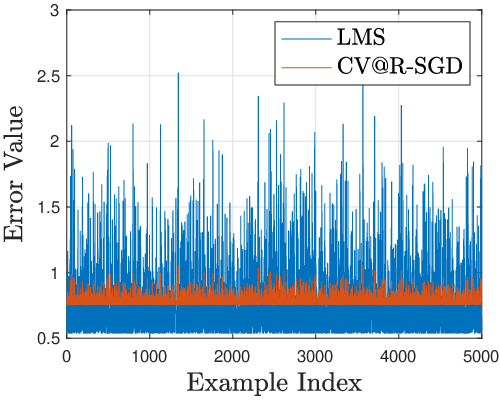
Figs. 7.1 and 7.2 show the iterate evolution as well as the behavior of the optimal prediction (test) error for both $\mathrm{CV@R}$-SGD (with stepsizes $\beta\equiv\alpha\hskip-1.00374pt\hskip-1.00374pt\times\hskip-1.00374pt\hskip-1.00374pt0.01$ and $\gamma\equiv 0.001$) and the LMS scheme (with stepsize $\beta\equiv 0.01$), respectively. We observe that both algorithms converge at an essentially identical noisy linear rate, in line with Theorem 1. However, the solutions are radically different. In fact, the risk-aware solution discovered by $\mathrm{CV@R}$-SGD dramatically reduces the volatility of prediction error, and provides prediction stability. Although this apparently comes at the cost sacrificing mean performance, such sacrifice is fully user-customizable by varying the $\mathrm{CV@R}$ level $\alpha$.

Figure 7.2: Comparison between risk-neutral (LMS) and risk-aware ($\mathrm{CV@R}$-SGD) ridge regression: Histogram (left) and actual values (right) of the test error.

8 Conclusion

In this work, we established noisy linear convergence of SGD for sequential $\mathrm{CV@R}$ learning, for a large class of possibly nonconvex loss functions satisfying a set-restricted PŁ inequality, also including all smooth and strongly convex losses as special cases. This result disproves the belief that $\mathrm{CV@R}$ learning is fundamentally difficult, and shows that classical learning problems can be solved efficiently under $\mathrm{CV@R}$ criteria, just as their risk-neutral versions. Our theory was also illustrated via an indicative numerical example. Future work includes the consideration of special learning settings such as linear least squares, as well as other risk measures beyond $\mathrm{CV@R}$.

References

- Bennis et al. [2018] Mehdi Bennis, Merouane Debbah, and H. Vincent Poor. Ultrareliable and Low-Latency Wireless Communication: Tail, Risk, and Scale. Proceedings of the IEEE, 106(10):1834–1853, October 2018. ISSN 15582256. 10.1109/JPROC.2018.2867029.
- Cardoso and Xu [2019] Adrian Rivera Cardoso and Huan Xu. Risk-Averse Stochastic Convex Bandit. In International Conference on Artificial Intelligence and Statistics, volume 89, pages 39–47, April 2019.
- Chaccour et al. [2020] Christina Chaccour, Mehdi Naderi Soorki, Walid Saad, Mehdi Bennis, and Petar Popovski. Risk-Based Optimization of Virtual Reality over Terahertz Reconfigurable Intelligent Surfaces. In IEEE International Conference on Communications, volume 2020-June. Institute of Electrical and Electronics Engineers Inc., June 2020. ISBN 9781728150895. 10.1109/ICC40277.2020.9149411.
- Curi et al. [2019] Sebastian Curi, Kfir. Y. Levy, Stefanie Jegelka, and Andreas Krause. Adaptive Sampling for Stochastic Risk-Averse Learning. arXiv preprint, arXiv:1910.12511, October 2019.
- Gotoh and Takeda [2016] Jun Ya Gotoh and Akiko Takeda. CVaR Minimizations in Support Vector Machines. In Financial Signal Processing and Machine Learning, pages 233–265. John Wiley & Sons, Ltd, Chichester, UK, April 2016. ISBN 9781118745540. 10.1002/9781118745540.ch10.
- Gürbüzbalaban et al. [2020] Mert Gürbüzbalaban, Andrzej Ruszczyński, and Landi Zhu. A Stochastic Subgradient Method for Distributionally Robust Non-Convex Learning. arXiv preprint, arXiv:2006.04873, June 2020.
- Huang and Haskell [2018] Wenjie Huang and William B. Haskell. Risk-Aware Q-learning for Markov Decision Processes. In 2017 IEEE 56th Annual Conference on Decision and Control, CDC 2017, volume 2018-Janua, pages 4928–4933. IEEE, December 2018. ISBN 9781509028733. 10.1109/CDC.2017.8264388.
- Kalogerias and Powell [2018] Dionysios S. Kalogerias and Warren B. Powell. Recursive Optimization of Convex Risk Measures: Mean-Semideviation Models. arXiv preprint, arXiv:1804.00636, April 2018.
- Karimi et al. [2016] Hamed Karimi, Julie Nutini, and Mark Schmidt. Linear Convergence of Gradient and Proximal-Gradient Methods under the Polyak-Łojasiewicz Condition. In Machine Learning and Knowledge Discovery in Databases, ECML PKDD 2016, Lecture Notes in Computer Science, volume 9851 LNAI, pages 795–811. Springer Verlag, 2016. ISBN 9783319461274. 10.1007/978-3-319-46128-1_50.
- Kim et al. [2019] Sung-Kyun Kim, Rohan Thakker, and Ali-akbar Agha-mohammadi. Bi-directional Value Learning for Risk-aware Planning Under Uncertainty. IEEE Robotics and Automation Letters, 4(3):2493–2500, July 2019. ISSN 2377-3766. 10.1109/LRA.2019.2903259.
- Koppel et al. [2019] Alec Koppel, Amrit S. Bedi, and Ketan Rajawat. Controlling the Bias-Variance Tradeoff via Coherent Risk for Robust Learning with Kernels. In Proceedings of the American Control Conference, volume 2019-July, pages 3519–3525. Institute of Electrical and Electronics Engineers Inc., July 2019. ISBN 9781538679265. 10.23919/acc.2019.8814879.
- Kushner and Yin [2003] Harold J. (Harold Joseph) Kushner and George Yin. Stochastic Approximation and Recursive Algorithms and Applications. Springer, 2003. ISBN 9780387008943.
- Lee et al. [2020] Jaeho Lee, Sejun Park, and Jinwoo Shin. Learning Bounds for Risk-sensitive Learning. arXiv preprint, arXiv:2006.08138, June 2020.
- Li et al. [2020] Yan Li, Deke Guo, Yawei Zhao, Xiaofeng Cao, and Honghui Chen. Efficient Risk-Averse Request Allocation for Multi-Access Edge Computing. IEEE Communications Letters, pages 1–1, September 2020. ISSN 1089-7798. 10.1109/lcomm.2020.3027562.
- Ma et al. [2018] Wann-Jiun Ma, Chanwook Oh, Yang Liu, Darinka Dentcheva, and Michael M. Zavlanos. Risk-Averse Access Point Selection in Wireless Communication Networks. IEEE Transactions on Control of Network Systems, 5870(c):1–1, 2018. ISSN 2325-5870. 10.1109/TCNS.2018.2792309.
- Markowitz [1952] Harry Markowitz. Portfolio Selection. The Journal of Finance, 7(1):77–91, March 1952. ISSN 15406261. 10.1111/j.1540-6261.1952.tb01525.x.
- Mhammedi et al. [2020] Zakaria Mhammedi, Benjamin Guedj, and Robert C. Williamson. PAC-Bayesian Bound for the Conditional Value at Risk. arXiv preprint, arXiv:2006.14763, June 2020.
- Polyak [1963] B. T. Polyak. Gradient Methods for Minimizing Functionals. USSR Computational Mathematics and Mathematical Physics, 3(4):864–878, January 1963. ISSN 00415553. 10.1016/0041-5553(63)90382-3.
- Rockafellar and Uryasev [2000] R. Tyrrell Rockafellar and Stanislav Uryasev. Optimization of Conditional Value-at-Risk. Journal of Risk, 2:21–41, 2000. ISSN 10769986. 10.2307/1165345.
- Schölkopf et al. [2000] Bernhard Schölkopf, Alex J. Smola, Robert C. Williamson, and Peter L. Bartlett. New Support Vector Algorithms. Neural Computation, 12(5):1207–1245, March 2000. ISSN 08997667. 10.1162/089976600300015565.
- Shapiro et al. [2014] Alexander Shapiro, Darinka Dentcheva, and Andrzej Ruszczyński. Lectures on Stochastic Programming: Modeling and Theory. Society for Industrial and Applied Mathematics, 2nd edition, 2014. ISBN 089871687X. http://dx.doi.org/10.1137/1.9780898718751.
- Soma and Yoshida [2020] Tasuku Soma and Yuichi Yoshida. Statistical Learning with Conditional Value at Risk. arXiv preprint, arXiv:2002.05826, February 2020.
- Takeda and Kanamori [2009] Akiko Takeda and Takafumi Kanamori. A Robust Approach Based on Conditional Value-at-Risk Measure to Statistical Learning Problems. European Journal of Operational Research, 198(1):287–296, October 2009. ISSN 03772217. 10.1016/j.ejor.2008.07.027.
- Takeda and Sugiyama [2008] Akiko Takeda and Masashi Sugiyama. -Support Vector Machine as Conditional Value-at-Risk Minimization. In Proceedings of the 25th International Conference on Machine Learning, pages 1056–1063, New York, New York, USA, 2008. Association for Computing Machinery (ACM). ISBN 9781605582054. 10.1145/1390156.1390289.
- Vapnik [2000] Vladimir N. Vapnik. The Nature of Statistical Learning Theory. Springer, 2000. ISBN 0387987800.
- Vitt et al. [2019] Constantine Alexander Vitt, Darinka Dentcheva, and Hui Xiong. Risk-Averse Classification. Annals of Operations Research, August 2019. ISSN 0254-5330. 10.1007/s10479-019-03344-6.
- Williamson and Menon [2019] Robert C Williamson and Aditya Krishna Menon. Fairness Risk Measures. In 36th International Conference on Machine Learning, ICML 2019, volume 2019-June, pages 11763–11774, 2019. ISBN 9781510886988.
- Zhou and Tokekar [2020] Lifeng Zhou and Pratap Tokekar. An Approximation Algorithm for Risk-Averse Submodular Optimization. In Springer Proceedings in Advanced Robotics, vol. 14, pages 144–159. Springer, Cham, December 2020. 10.1007/978-3-030-44051-0_9.