A Comment on and Correction to: Opinion dynamics in the presence of increasing agreement pressure

Abstract

We identify a counter-example to the consensus result given in [J. Semonsen et al. Opinion dynamics in the presence of increasing agreement pressure. IEEE Trans. Cyber., 49(4): 1270-1278, 2018]. We resolve the counter-example by replacing Lemma 5 in the given reference with a novel variation of the Banach Fixed Point theorem which explains both the numerical results in the reference and the counter-example(s) in this note, and provides a sufficient condition for consensus in systems with increasing peer-pressure. This work is relevant for other papers that have used the proof technique from Semonsen et al. and establishes the veracity of their claims assuming the new sufficient condition.

1 Introduction

In this technical note we correct and clarify a consensus result given in [1]. This correction is relevant not only to the general literature but in particular to [2], which uses the same proof technique as [1] and [3, 4, 5, 6, 7, 8, 9, 10], which cite [1]. We show this proof method is incomplete due to the use of a lemma drawn from outside the consensus literature. We provide a complete result and use this to prove a corrected version of Theorem 2 in [1].

In [1], the authors study a consensus problem (see e.g., [11, 12, 13, 14, 15, 16, 17, 18, 19, 20, 21, 22, 23, 24, 25, 26, 27, 28, 29, 30, 31, 32, 33, 34, 35, 36, 37, 38, 39]) under an increasing peer-pressure function, which seems to drive system consensus. That paper assumes $N$ agents are arranged on a weighted graph with weighted adjacency matrix $\mathbf{A}\in\mathbb{R}^{N\times N}$ where self-weights are all $0$. Each agent has a time-varying state $x^{(i)}\in[0,1]$ (though any inputs in $\mathbb{R}$ would suffice) and the vector $\mathbf{x}_{k}\in\mathbb{R}^{N}$ is the vector of agent states at time $k$. Each agent also has a stubbornness coefficient $s^{(i)}$ (also used in [2]) and a preferred state ${x^{+^{(i)}}}$, which defines a fixed vector $\mathbf{x}^{+}\in\mathbb{R}^{N\times N}$. Define a diagonal matrix $\mathbf{S}$ containing the $s^{(i)}$ and a diagonal matrix $\mathbf{D}$ of row-sums of $\mathbf{A}$. The the update function studied in [1] is:

$$\mathbf{x}_{(k)}=\left(\mathbf{S}+\rho_{k}\mathbf{D}\right)^{-1}\left(\mathbf{S}\mathbf{x}^{+}+\rho_{k}\mathbf{A}\mathbf{x}_{(k-1)}\right).$$ (1)

Here $\rho_{k}$ is a time-varying peer-pressure value. Let:

$$f_{k}(\mathbf{x})=\left(\mathbf{S}+\rho_{k}\mathbf{D}\right)^{-1}\left(\mathbf{S}\mathbf{x}^{+}+\rho_{k}\mathbf{A}\mathbf{x}_{(k-1)}\right).$$ (2)

In Lemma 3 of [1] it is shown that $f_{k}(\mathbf{x})$ is a contraction with a fixed point:

$$\mathbf{x}_{k}^{*}=\left(\mathbf{S}+\rho_{k}\mathbf{L}\right)^{-1}\mathbf{S}\mathbf{x}^{+},$$

where: $\mathbf{L}=\mathbf{D}-\mathbf{A}$ is the Laplacian. It is noted in Theorem 1 of [1] that:

$$\lim_{k\to\infty}\mathbf{x}_{k}^{*}=\frac{\sum_{i=1}^{N}s_{i}x_{i}^{+}}{\sum_{i=1}^{N}s_{i}}{\bf 1}.$$ (3)

That is the fixed points of the individual contractions converge to the stubbornness weighted mean of the agents’ preferred states. The authors state Lemma 5, taken directly from [40, 41]:

Lemma 1.1 (Theorem 1 of [40] & Theorem 2 of [41]).

Let $\{f_{n}\}$ be a sequence of analytic contractions in a domain $D$ with $f_{n}(D)\subseteq E\subseteq D_{0}\subseteq D$ for all $n$. Then $F_{n}=f_{n}\circ f_{n-1}\circ\cdots\circ f_{1}$ converges uniformly in $D_{0}$ and locally uniformly in $D$ to a constant function $F(z)=c\in E$. Furthermore, the fixed points of $f_{n}$ converge to the constant $c$. ∎

[1] then uses this to argue (in Theorem 2) that when:

$$G_{k}(\mathbf{x})=(f_{k}\circ\cdots\circ f_{1})(\mathbf{x}),$$

if $\rho_{k}\to\infty$, then:

$$\lim_{k\to\infty}G_{k}(\mathbf{x}_{0})=\mathbf{x}^{*}.$$

In the next section, we show this is not a complete statement and that the system may fail to converge for certain choices of increasing $\rho_{k}$. The failure in this case is due to the use of Lemma 1.1 (Lemma 5 of [1]), which appears not to be valid in this case. We then prove a variation of the Banach fixed-point theorem, which explains our example’s failure to converge and provides a correct sufficient condition for convergence, thus completing Theorem 2 of [1].

2 Counter-Example to Consensus

Consider the simple graph $K_{2}$ with the following inputs:

$$\mathbf{A}=\begin{bmatrix}0&1\\ 1&0\end{bmatrix}\qquad\mathbf{S}=\mathbf{D}=\mathbf{I}_{2}$$

Let the initial condition and preferred agent states be given by $\mathbf{x}^{+}=\langle{0.1,0.5}\rangle$. Assume we define the exponentially increasing peer-pressure function:

$$\rho_{k}=2^{\sqrt{k}},$$

which provides some numerical stability (i.e., does not blow up too quickly) but also shows exponential growth. Simulation of Eq. 1 shows the system does not converge to the expected $\mathbf{x^{*}}=\langle{3,3}\rangle$ as given by Eq. 3, but instead oscillates about this point indefinitely. This is shown in Fig. 1.

(a) Initial Behavior

(b) Long Run Oscillation

Figure 1: Initially fast convergence around the mean point $\mathbf{x^{*}}=\langle{3,3}\rangle$ slows and becomes oscillation, showing neutral stability, rather than asymptotic stability.

However, if we replace the peer-pressure function with:

$$\rho_{k}=k,$$

then we see the system converges as expected from Theorem 1 of [1].

(a) Initial Behavior

(b) Long Run Oscillation

Figure 2: Asymptotic convergence to the point $\mathbf{x^{*}}=\langle{3,3}\rangle$ is illustrated. As noted in [1] this convergence is linear.

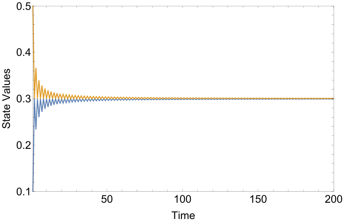
It is clear from this example that the issue with Theorem 1 is not the statement of the theorem, but its lack of qualification on the growth of $\rho_{k}$. This stems directly from Lemma 5 of [1] (or Theorem 1 of [40] & Theorem 2 of [41]), which also does not qualify the analytic contraction to be used. However, it is clear that this pathology is an example of an even easier example.

Consider the family of functions $f:\mathbb{R}\to\mathbb{R}$:

$$f_{k}(x)=\left(1-\frac{1}{10^{n}}\right)x.$$ (4)

Each $f_{k}(x)$ has a fixed point $x_{k}^{*}=0$, thus the fixed points $x_{k}^{*}$ converge to $x^{*}=0$ (tautologically). Moreover, each function contracts any interval containing $x=0$ into itself. However, computing:

$$G_{k}(x)=(f_{k}\circ f_{k-1}\circ\cdots\circ f_{1})(x)=\left(\prod_{i=1}^{k}\left(1-\frac{1}{10^{n}}\right)\right)x,$$

we see that:

$$\lim_{k\to\infty}G_{k}(x)=x\cdot\lim_{k\to\infty}\prod_{n=1}^{k}\left(1-\frac{1}{10^{n}}\right)=x\cdot\phi\left(\tfrac{1}{10}\right).$$

Here $\phi(\cdot)$ is Euler’s function derived from the q-Pochhammer symbol. We note that:

$$\phi\left(\tfrac{1}{10}\right)\approx 0.89001$$

Therefore, for $x\neq 0$, $G_{\infty}(x)\approx 0.89001x$, rather than $0$ as would be expected from the statement of Lemma 5 of [1]. By contrast, if we consider the family of functions:

$$f_{k}(x)=\frac{k-1}{k}x,$$ (5)

then:

$$G_{k}(x)=\left(\prod_{n=1}^{k}\frac{n-1}{n}\right)x$$

and

$$\lim_{k\to\infty}G_{k}(x)=x\cdot\lim_{k\to\infty}\left(\prod_{n=1}^{k}\frac{n-1}{n}\right)=0,$$

as expected. We note this counter-example can be extended to the complex plane (the domain used in Lemma 1.1). In this note, we will not consider the question of whether the statement of Lemma 1.1 needs to be clarified, however it may be that this result should be used with caution for future consensus results.

In the next section, we construct a variation of the Banach fixed point theorem that handles the conditions set forth in [1] and predicts the non-convergence of the counter-example using the intuition provided by the simpler cases.

3 A Convergence Theorem

Theorem 3.1.

Let $\{f_{i}\}_{i=1}^{\infty}$ be a family of mappings on a Banach space $X$ with norm $\left\lVert{\cdot}\right\rVert$ so that each mapping $f_{i}$ has a unique fixed point $\mathbf{x}_{i}^{*}$ satisfying the property:

$$\left\lVert{f_{i}(\mathbf{x})-\mathbf{x}_{i}^{*}}\right\rVert\leq\alpha_{i}\left\lVert{\mathbf{x}-\mathbf{x}_{i}^{*}}\right\rVert\qquad\forall\mathbf{x}\in X,$$

where $0\leq\alpha_{i}<1$ for all $i$. Furthermore, suppose that:

$$\lim_{i\to\infty}\mathbf{x}_{i}^{*}=\mathbf{x}^{*}\in X$$

Then, if $\mathbf{x}_{0}\in X$ and

$$\lim_{N\to\infty}\prod_{i=1}^{N}\alpha_{i}=0,$$

then:

$$\lim_{k\to\infty}(f_{k}\circ f_{k-1}\circ\cdots\circ f_{1})(\mathbf{x}_{0})=\mathbf{x}^{*}$$

Proof.

Define:

$$G_{k}=f_{k}\circ f_{k-1}\circ\cdots\circ f_{1}.$$

By assumption:

$$\left\lVert{(f_{k+1}\circ G_{k})(\mathbf{x}_{0})-\mathbf{x}_{k+1}^{*}}\right\rVert\leq\alpha_{k+1}\left\lVert{G_{k}(\mathbf{x}_{0})-\mathbf{x}_{k+1}^{*}}\right\rVert=\alpha_{k+1}\left\lVert{(f_{k}\circ G_{k-1})(\mathbf{x}_{0})-\mathbf{x}_{k+1}^{*}}\right\rVert.$$

Applying the triangle inequality to the last term we have:

$$\left\lVert{(f_{k+1}\circ G_{k})(\mathbf{x}_{0})-\mathbf{x}_{k+1}^{*}}\right\rVert\leq\alpha_{k+1}\left(\left\lVert{(f_{k}\circ G_{k-1})(\mathbf{x}_{0})-\mathbf{x}_{k}^{*}}\right\rVert+\left\lVert{\mathbf{x}_{k+1}^{*}-\mathbf{x}_{k}^{*}}\right\rVert\right).$$

Applying similar logic, we see that:

$$\left\lVert{(f_{k+1}\circ G_{k})(\mathbf{x}_{0})-\mathbf{x}_{k+1}^{*}}\right\rVert\leq\alpha_{k+1}\alpha_{k}\left\lVert{G_{k-1}(\mathbf{x}_{0})-\mathbf{x}_{k}^{*}}\right\rVert+\alpha_{k+1}\left\lVert{\mathbf{x}_{k+1}^{*}-\mathbf{x}_{k}^{*}}\right\rVert$$

Repeating this argument, we see:

$$\left\lVert{(f_{k+1}\circ G_{k})(\mathbf{x}_{0})-\mathbf{x}_{k+1}^{*}}\right\rVert\leq\\ \alpha_{k+1}\alpha_{k}\alpha_{k-1}\left\lVert{G_{k-2}(\mathbf{x}_{0})-\mathbf{x}_{k-1}^{*}}\right\rVert+\\ \alpha_{k+1}\alpha_{k}\left\lVert{\mathbf{x}_{k}^{*}-\mathbf{x}_{k-1}^{*}}\right\rVert+\alpha_{k+1}\left\lVert{\mathbf{x}_{k+1}^{*}-\mathbf{x}_{k}^{*}}\right\rVert$$

We can continue in this way until we see that:

$$\left\lVert{(f_{k+1}\circ G_{k})(\mathbf{x}_{0})-\mathbf{x}_{k+1}^{*}}\right\rVert\leq\left(\prod_{i=1}^{k+1}\alpha_{i}\right)\left\lVert{f_{1}(\mathbf{x}_{0})-\mathbf{x}_{1}^{*}}\right\rVert+\\ \sum_{j=1}^{k}\left(\prod_{i={j+1}}^{k+1}\alpha_{i}\right)\left\lVert{\mathbf{x}_{j+1}^{*}-\mathbf{x}_{j}^{*}}\right\rVert.$$ (6)

By assumption of the theorem, the fixed points $\mathbf{x}_{i}^{*}$ converge and therefore for any $\epsilon>0$ there is an $N>0$ so that:

$$\left\lVert{\mathbf{x}_{N}^{*}-\mathbf{x}_{N+1}^{*}}\right\rVert\leq\epsilon.$$ (7)

Suppose we are given an $\epsilon>0$, choose $N$ so that:

1. $$\left(\prod_{i=1}^{k+1}\alpha_{i}\right)\left\lVert{f_{1}(\mathbf{x}_{0})-\mathbf{x}_{1}^{*}}\right\rVert<\frac{\epsilon}{2(N+1)}.$$

   This is possible since we assume:

   $$\lim_{N\to\infty}\prod_{i=1}^{N}\alpha_{i}=0,$$ (8)

   and

   $$\lim_{N\to\infty}\left\lVert{\mathbf{x}_{N+1}-\mathbf{x}_{N}}\right\rVert=0.$$ (9)

2. For each $k$,

   $$\left(\prod_{i={j+1}}^{N+1}\alpha_{i}\right)\left\lVert{\mathbf{x}_{j+1}^{*}-\mathbf{x}_{j}^{*}}\right\rVert<\frac{\epsilon}{2(N+1)}.$$

   This is possible because of the combination of Eqs. 9 and 8.

3. $$\left\lVert{\mathbf{x}_{N+1}^{*}-\mathbf{x}^{*}}\right\rVert<\frac{\epsilon}{2}$$

Then from Eq. 6 we have:

$$\left\lVert{G_{n+1}(\mathbf{x}_{0})-\mathbf{x}_{n+1}^{*}}\right\rVert<\frac{\epsilon}{2}.$$

By one more application of the triangle inequality, we have:

$$\left\lVert{G_{n+1}(\mathbf{x}_{0})-\mathbf{x}^{*}}\right\rVert\leq\left\lVert{\mathbf{x}_{N+1}^{*}-\mathbf{x}^{*}}\right\rVert+\left\lVert{G_{n+1}(\mathbf{x}_{0})-\mathbf{x}_{n+1}^{*}}\right\rVert<\epsilon$$

This completes the proof. ∎

This theorem explains, as special cases, the families of functions defined in Eq. 4 and Eq. 5. In the next section, we use it to resolve the counter-example discussed in Section 2.

4 Resolution of the Counter Example

Returning to the example in Section 2, let $\mathbf{x}^{+}=\langle{a,b}\rangle$, thus generalizing the initial condition. In this case, Eq. 1 can be written as:

$$f_{k}(\mathbf{x})=\begin{bmatrix}\frac{(\rho+1)(a+\rho x_{2})}{\rho^{2}+2\rho+1}\\ \frac{(\rho+1)(b+\rho x_{1})}{\rho^{2}+2\rho+1}\end{bmatrix}.$$ (10)

For each $f_{k}(\mathbf{x})$ the explicit fixed point is given by:

$$\mathbf{x}_{k}^{*}=\begin{bmatrix}x_{1}^{*}\\ x_{2}^{*}\end{bmatrix}=\begin{bmatrix}\frac{a+\rho(a+b)}{2\rho+1}\\ \frac{b+\rho(a+b)}{2\rho+1}\end{bmatrix}.$$ (11)

Since $\langle{s_{1},s_{2}}\rangle=\langle{1,1}\rangle$, we see that:

$$\lim_{k\to\infty}\mathbf{x}_{k}^{*}=\mathbf{x}^{*}=\begin{bmatrix}\tfrac{1}{2}\\ \tfrac{1}{2}\end{bmatrix},$$

as expected.

Because this example is particularly simple, we can compute (see Appendix A):

$$\left\lVert{F(\mathbf{x})-\mathbf{x}_{k}^{*}}\right\rVert^{2}=\left(\frac{\rho_{k}}{1+\rho_{k}}\right)^{2}\left\lVert{\mathbf{x}-\mathbf{x}_{k}^{*}}\right\rVert^{2},$$ (12)

for any $\mathbf{x}$. In Theorem 3.1, we now have:

$$\alpha_{k}=\frac{\rho_{k}}{1+\rho_{k}}.$$

When $\rho_{k}=2^{\sqrt{k}}$, then:

$$\prod_{k=1}^{\infty}\alpha_{k}\approx 0.0310128>0,$$

which implies (as expected) that the system may not converge to the fixed point (see Fig. 1). On the other hand, when $\rho_{k}=k$,

$$\prod_{k=1}^{\infty}\alpha_{k}=0$$

ensuring that the system will converge to the weighted average of $\mathbf{x}^{+}$. Thus we can correct Theorem 2 of [1] to read:

Theorem 4.1 (Clarification of Theorem 2 of [1]).

Let

$$f_{k}(\mathbf{x})=\left(\mathbf{S}+\rho^{(k)}\mathbf{D}\right)^{-1}\left(\mathbf{S}\mathbf{x}^{+}+\rho^{(k)}\mathbf{A}\mathbf{x}\right).$$

Define:

$$\mathbf{x}_{k}=f_{k}(\mathbf{x}_{k-1}),$$

with $\mathbf{x}_{0}$ given (and assumed to be $\mathbf{x}^{+}$). If $\rho_{k}\to\infty$ and the resulting contraction constants $\alpha_{k}$ of $f_{k}$ satisfy:

$$\prod_{k=1}^{\infty}\alpha_{k}=0,$$

then

$$\lim_{k\to\infty}\mathbf{x}_{k}=\frac{\sum_{i}s_{i}\mathbf{x}_{k_{i}}}{\sum_{i}s_{i}}.$$

∎

As a final remark, we note that this result could be anticipated from the convergence rate analysis in [1], which shows that Eq. 1 is an instance of gradient descent. Convergence guarantees for such an algorithm require satisfaction of the Wolfe Conditions and several pathological examples exist in which the step length (governed by $\rho_{k}$) is improperly defined leading to oscillation in gradient descent (see [42]). Thus, one might view Theorem 4.1 as a specialized sufficient condition on step length in this gradient descent.

5 Conclusions

In this technical note, we corrected and clarified Theorem 2 of [1]. This correction is important because the proof method has been used by other authors [2]. The correction is based on replacing a lemma (Lemma 5) used in [1] with a new variation on the Banach Fixed Point theorem. The modified theorem(s) now ensure results in [1] and [2] can be used for development of consensus systems or for their further study.

Appendix A Computation of the Norms

Computing directly we have:

$$\left\lVert{f_{k}(\mathbf{x})-\mathbf{x}_{k}^{*}}\right\rVert^{2}=\left(\frac{a+\rho x_{2}}{\rho+1}-\frac{a+\rho(a+b)}{2\rho+1}\right)^{2}+\\ \left(\frac{b+\rho x_{1}}{\rho+1}-\frac{b+\rho(a+b)}{2\rho+1}\right)^{2}$$

We also have:

$$\left\lVert{\mathbf{x}-\mathbf{x}_{k}^{*}}\right\rVert^{2}=\left(x_{1}-\frac{\rho(a+b)+a}{2\rho+1}\right)^{2}+\\ \left(x_{2}-\frac{\rho(a+b)+b}{2\rho+1}\right)^{2}.$$

Dividing these expressions into each other and simplifying yields Eq. 12.

References

- [1] Justin Semonsen, Christopher Griffin, Anna Squicciarini, and Sarah Rajtmajer. Opinion dynamics in the presence of increasing agreement pressure. IEEE transactions on cybernetics, 49(4):1270–1278, 2018.
- [2] Guang He, Wenbing Zhang, Jing Liu, and Haoyue Ruan. Opinion dynamics with the increasing peer pressure and prejudice on the signed graph. Nonlinear Dynamics, pages 1–13, 2020.
- [3] Hyo-Sung Ahn, Quoc Van Tran, Minh Hoang Trinh, Kevin L Moore, Mengbin Ye, and Ji Liu. Cooperative opinion dynamics on multiple interdependent topics: Modeling and analysis. arXiv preprint arXiv:1807.04406, 2018.
- [4] Mingjun Du, Baoli Ma, and Deyuan Meng. Edge convergence problems on signed networks. IEEE transactions on cybernetics, 49(11):4029–4041, 2018.
- [5] Zihan Chen, Jiahu Qin, Bo Li, Hongsheng Qi, Peter Buchhorn, and Guodong Shi. Dynamics of opinions with social biases. Automatica, 106:374–383, 2019.
- [6] Haiming Liang, Cong-Cong Li, Guoyin Jiang, and Yucheng Dong. Preference evolution model based on wechat-like interactions. Knowledge-Based Systems, 185:104998, 2019.
- [7] Yilun Shang. Resilient consensus for expressed and private opinions. IEEE Transactions on Cybernetics, 2019.
- [8] Haoti Zhong, Hao Li, Anna Squicciarini, Sarah Rajtmajer, and David Miller. Toward image privacy classification and spatial attribution of private content. In 2019 IEEE International Conference on Big Data (Big Data), pages 1351–1360. IEEE, 2019.
- [9] Qinyue Zhou, Zhibin Wu, Abdulrahman H Altalhi, and Francisco Herrera. A two-step communication opinion dynamics model with self-persistence and influence index for social networks based on the degroot model. Information Sciences, 519:363–381, 2020.
- [10] Hyo-Sung Ahn, Quoc Van Tran, Minh Hoang Trinh, Mengbin Ye, Ji Liu, and Kevin L Moore. Opinion dynamics with cross-coupling topics: Modeling and analysis. IEEE Transactions on Computational Social Systems, 2020.
- [11] M. H. DeGroot. Reaching a consensus. J. American Stat. Association, 69:118–121, 1974.
- [12] U. Krause. A discrete nonlinear and non-autonomous model of consensus formation. In Gordon and Breach, editors, In Communications in Difference Equations, pages 227– 236, 2000.
- [13] V. D. Blondel, J. M. Hendrickx, A. Olshevsky, and J. N. Tsitsiklis. Convergence in multiagent coordination, consensus, and flocking. In Proceedings of the 44th IEEE Conference on Decision and Control, pages 2996–3000, Dec 2005.
- [14] R. Olfati-Saber, J. A. Fax, and R. M. Murray. Consensus and cooperation in networked multi-agent systems. Proceedings of the IEEE, 95(1):215–233, Jan 2007.
- [15] V. D. Blondel, J. M. Hendrickx, and J. N. Tsitsiklis. On krause’s multi-agent consensus model with state-dependent connectivity. IEEE Transactions on Automatic Control, 54(11):2586–2597, Nov 2009.
- [16] C. Canuto, F. Fagnani, and P. Tilli. An eulerian approach to the analysis of krause’s consensus models. SIAM J. Contr. and Opt., pages 243–265, 2012.
- [17] Pierre-Emmanuel Jabin and Sebastien Motsch. Clustering and asymptotic behavior in opinion formation. Journal of Differential Equations, 257(11):4165 – 4187, 2014.
- [18] S. Motsch and E. Tadmor. Heterophilious Dynamics Enhances Consensus. SIAM Review, 56:577–621, 2014.
- [19] David Bindel, Jon Kleinberg, and Sigal Oren. How bad is forming your own opinion? Games and Economic Behavior, 92:248 – 265, 2015.
- [20] Y. Wu, H. Su, P. Shi, Z. Shu, and Z. G. Wu. Consensus of multiagent systems using aperiodic sampled-data control. IEEE Transactions on Cybernetics, 46(9):2132–2143, Sept 2016.
- [21] J. He, M. Zhou, P. Cheng, L. Shi, and J. Chen. Consensus under bounded noise in discrete network systems: An algorithm with fast convergence and high accuracy. IEEE Transactions on Cybernetics, 46(12):2874–2884, Dec 2016.
- [22] C. Hua, X. You, and X. Guan. Adaptive leader-following consensus for second-order time-varying nonlinear multiagent systems. IEEE Transactions on Cybernetics, 47(6):1532–1539, June 2017.
- [23] W. Meng, Q. Yang, J. Si, and Y. Sun. Consensus control of nonlinear multiagent systems with time-varying state constraints. IEEE Transactions on Cybernetics, 47(8):2110–2120, Aug 2017.
- [24] Y. Chen and Y. Shi. Consensus for linear multiagent systems with time-varying delays: A frequency domain perspective. IEEE Transactions on Cybernetics, 47(8):2143–2150, Aug 2017.
- [25] X. Xu, L. Liu, and G. Feng. Consensus of heterogeneous linear multiagent systems with communication time-delays. IEEE Transactions on Cybernetics, 47(8):1820–1829, Aug 2017.
- [26] X. Ge and Q. L. Han. Consensus of multiagent systems subject to partially accessible and overlapping markovian network topologies. IEEE Transactions on Cybernetics, 47(8):1807–1819, Aug 2017.
- [27] H. Rezaee and F. Abdollahi. Consensus problem over high-order multiagent systems with uncertain nonlinearities under deterministic and stochastic topologies. IEEE Transactions on Cybernetics, 47(8):2079–2088, Aug 2017.
- [28] Y. Wei and G. P. Liu. Consensus tracking of heterogeneous discrete-time networked multiagent systems based on the networked predictive control scheme. IEEE Transactions on Cybernetics, 47(8):2173–2184, Aug 2017.
- [29] H. Li, C. Huang, G. Chen, X. Liao, and T. Huang. Distributed consensus optimization in multiagent networks with time-varying directed topologies and quantized communication. IEEE Transactions on Cybernetics, 47(8):2044–2057, Aug 2017.
- [30] Q. Song, F. Liu, G. Wen, J. Cao, and X. Yang. Distributed position-based consensus of second-order multiagent systems with continuous/intermittent communication. IEEE Transactions on Cybernetics, 47(8):1860–1871, Aug 2017.
- [31] L. Xing, C. Wen, F. Guo, Z. Liu, and H. Su. Event-based consensus for linear multiagent systems without continuous communication. IEEE Transactions on Cybernetics, 47(8):2132–2142, Aug 2017.
- [32] L. Zou, Z. Wang, H. Gao, and F. E. Alsaadi. Finite-horizon consensus control of time-varying multiagent systems with stochastic communication protocol. IEEE Transactions on Cybernetics, 47(8):1830–1840, Aug 2017.
- [33] C. Hua, Y. Li, and X. Guan. Leader-following consensus for high-order nonlinear stochastic multiagent systems. IEEE Transactions on Cybernetics, 47(8):1882–1891, Aug 2017.
- [34] Z. Zhang, L. Zhang, F. Hao, and L. Wang. Leader-following consensus for linear and lipschitz nonlinear multiagent systems with quantized communication. IEEE Transactions on Cybernetics, 47(8):1970–1982, Aug 2017.
- [35] Z. Yu, H. Jiang, C. Hu, and J. Yu. Necessary and sufficient conditions for consensus of fractional-order multiagent systems via sampled-data control. IEEE Transactions on Cybernetics, 47(8):1892–1901, Aug 2017.
- [36] K. Liu, Z. Ji, and W. Ren. Necessary and sufficient conditions for consensus of second-order multiagent systems under directed topologies without global gain dependency. IEEE Transactions on Cybernetics, 47(8):2089–2098, Aug 2017.
- [37] L. Ding and W. X. Zheng. Network-based practical consensus of heterogeneous nonlinear multiagent systems. IEEE Transactions on Cybernetics, 47(8):1841–1851, Aug 2017.
- [38] J. Qin, W. Fu, W. X. Zheng, and H. Gao. On the bipartite consensus for generic linear multiagent systems with input saturation. IEEE Transactions on Cybernetics, 47(8):1948–1958, Aug 2017.
- [39] W. Hu, L. Liu, and G. Feng. Output consensus of heterogeneous linear multi-agent systems by distributed event-triggered/self-triggered strategy. IEEE Transactions on Cybernetics, 47(8):1914–1924, Aug 2017.
- [40] L. Lorentzen. Compositions of contractions. J. Computational and Applied Mathematics, 32:169–178, 1990.
- [41] John Gill. The use of the sequence in computing fixed points of continued fractions, products, and series. Applied Numerical Mathematics, 8(6):469 – 476, 1991.
- [42] D. P. Bertsekas. Nonlinear Programming. Athena Scientific, 2 edition, 1999.