A Theory for Backtrack-Downweighted Walks

Abstract

We develop a complete theory for the combinatorics of walk-counting on a directed graph in the case where each backtracking step is downweighted by a given factor. By deriving expressions for the associated generating functions, we also obtain linear systems for computing centrality measures in this setting. In particular, we show that backtrack-downweighted Katz-style network centrality can be computed at the same cost as standard Katz. Studying the limit of this centrality measure at its radius of convergence also leads to a new expression for backtrack-downweighted eigenvector centrality that generalizes previous work to the case where directed edges are present. The new theory allows us to combine advantages of standard and nonbacktracking cases, avoiding localization while accounting for tree-like structures. We illustrate the behaviour of the backtrack-downweighted centrality measure on both synthetic and real networks.

1 Motivation

1.1 Nonbacktracking Walks

Many concepts in network science are built on the notion of walks. We may study the transient or long term behaviour of random walks of a certain form. Or we may consider the combinatorics of all distinct walks of a given type. Such ideas, which lie at intersection between graph theory, combinatorics and applied linear algebra, form the basis of effective algorithms for summarizing network properties [20, 27].

Our focus here is on the definition and analysis of a new type of combinatoric walk-count which interpolates between the classical and nonbacktracking cases. In the classical setting, a walker may continue by traversing any edge pointing out of the current node. In the nonbacktracking setting, the walker must never continue along the reverse of the edge on which they arrived. Intuitively, eliminating backtracking forces the walker to explore the network more widely. More concretely, it has been shown to offer benefits in centrality measurement [2, 3, 9, 14, 22, 29, 38], community detection [19, 21, 28, 30, 32], network comparison and alignment [23, 39] and in the study of related issues concerning optimal percolation [25, 26] and the spread of epidemics [24].

Nonbacktracking also plays an important role in a number of seemingly unrelated scientific fields, including spectral graph theory [1, 16], number theory [37], discrete mathematics [7, 17, 35], quantum chaos [33], random matrix theory [34], and computer science [31, 40]. Hence, our results also have potential for impact outside network science.

1.2 Downweighting rather than Eliminating

Our work can be motivated by two issues

a.

Treating all walks equally leads to centrality measures that suffer from localization—placing most emphasis on a small subset of nodes and struggling to distinguish between the remainder. This issue can be associated with an accumulation of backtracking walks [2, 22].

b.

Completely eliminating backtracking walks, however, may overlook some features, notably the existence of trees [28].

For this reason, we will consider a more general regime where any backtracking step during a walk is downweighted by some factor, $0\leq\theta\leq 1$. So the extremes of $\theta=1$ and $\theta=0$ correspond to standard and nonbacktracking walk counts, respectively.

We are concerned with the combinatorics of such backtrack-downweighted walks—we seek a formula for the number of distinct walks of each length in a given graph. We then study the associated generating functions in order to produce Katz-style network centrality measures. Moreover, by considering how the resolvent-based generating function behaves at its radius of convergence, we also arrive at a corresponding eigenvector centrality.

We note that in [9] the related concept of alpha-nonbacktracking centrality was introduced. That work focused on the eigenvector setting, adapting the Hashimoto matrix construction, and applied only to undirected networks. Our work allows for directed networks and is built on a combinatoric walk-counting approach that generalizes Katz centrality. Further, by working at the node level rather than the edge level, we are able to derive more computationally efficient measures, based on linear systems with the same dimension and sparsity as the original network.

We finish this section by describing how the manuscript is organized, and pointing out how previous results are generalized. In section 2 we introduce the required background concepts. Section 3 defines backtrack-downweighted walks and in Theorem 3.1 we derive a general four-term recurrence that allows us to count them. This result extends the fully nonbacktracking version from [7]; see also [36]. Section 4 concerns the standard generating function. Corollary 4.2 gives a linear system for the associated Katz-style centrality measure, generalizing [2, equation (3.3)]. In section 5 we give results on a small graph that illustrate the two motivational issues a and b above. (This graph has an interesting spectral property that is described in Remark 5.1.) We also give comparative results on the star graph and on regular graphs. In section 6 we consider the limit as the Katz parameter approaches its upper value, and thereby, in Theorem 6.3, derive an eigenvector centrality measure. This result extends the measure in [9] to the case of directed graphs. Section 7 shows how the recurrence from Theorem 3.1 can be used to compute generating functions based on general power series. Here we find it necessary to work with block matrices of three times the dimension of the original adjacency matrix; see Theorem 7.1, which extends [3, Theorem 5.2]. In section 8 we give results on data from the London Underground train network, and we argue that the backtrack-downweighting parameter provides a useful means to mitigate localization while maintaining correlation with passenger usage. We finish with a brief discussion in section 9.

2 Background and Notation

We consider an unweighted, directed network with $n$ nodes. We let $A\in\mathbb{R}^{n\times n}$ denote the adjacency matrix, so $a_{ij}=1$ if there is an edge from $i$ to $j$ and $a_{ij}=0$ otherwise. There are no self-loops, so $a_{ii}=0$. A walk of length $k$ from node $i$ to node $j$ is a sequence of nodes $i=i_{0},i_{1},i_{2},\ldots,i_{k}=j$ such that each edge from $i_{s}$ to $i_{s+1}$ exists. Note that the nodes in the sequence are not required to be distinct; the walk may revisit nodes and edges. It follows directly from the definition of matrix multiplication that $(A^{k})_{ij}$ counts the number of distinct walks of length $k$ from $i$ to $j$ [20].

Katz [18] used this walk-counting expression as the basis for a centrality measure. Here, we compute a value $x_{i}>0$ that quantifies the importance of node $i$, with a larger value indicating greater importance. Katz centrality uses

$$x_{i}=1+\sum_{k=1}^{\infty}\sum_{j=1}^{n}\alpha^{k}(A^{k})_{ij}.$$ (1)

Here, (up to a convenient constant unit shift) the centrality of node $i$ is given by the total number of walks from node $i$ to every node, with a walk of length $k$ weighted by a factor $\alpha^{k}$, where $\alpha>0$ is a real parameter. This series converges for $\alpha<1/\rho(A)$, where $\rho(\cdot)$ denotes the spectral radius, and we may use the matrix-vector notation

$$(I-\alpha A)\mathbf{x}=\mathbf{1},$$ (2)

where $\mathbf{1}\in\mathbb{R}^{n}$ has all elements equal to one.

A nonbacktracking walk of length $k$ from node $i$ to node $j$ is a sequence of nodes $i=i_{0},i_{1},i_{2},\ldots,i_{k}=j$ such that each edge from $i_{s}$ to $i_{s+1}$ exists and we never have $i_{s}=i_{s+2}$. In words, after leaving a node we must not return to it immediately. Now, let $p_{k}(A)\in\mathbb{R}^{n\times n}$ be such that $(p_{k}(A))_{ij}$ records the number of distinct nonbacktracking walks of length $k$ from $i$ to $j$. It is straightforward to show that

$$p_{1}(A)=A,\quad\text{and}\quad p_{2}(A)=A^{2}-D,$$

where $D\in\mathbb{R}^{n\times n}$ is the diagonal matrix whose entries are $d_{ii}=(A^{2})_{ii}$. Setting $p_{0}(A)=I$ for convenience, it was shown in [7] that the matrices $p_{k}(A)$ satisfy the following four-term recurrence

$$p_{k+1}(A)=p_{k}(A)A+p_{k-1}(A)(I-D)-p_{k-2}(A)(A-S),\quad\text{for~}k=2,3,\ldots,$$ (3)

where $S\in\mathbb{R}^{n\times n}$ is such that $s_{ij}=a_{ij}a_{ji}$. See [36] for an alternative, linear algebraic, proof.

We note that in the extreme case of a directed network for which no edges are reciprocated, that is $a_{ij}=1\Rightarrow a_{ji}=0$, there is no opportunity for any walk to backtrack; all walks are nonbacktracking. In this case, we have $D=0$ and $S=0$, and $p_{k}(A)$ recovers the classical walk count $A^{k}$.

Motivated by (1), the nonbacktracking Katz analogue

$$x_{i}=1+\sum_{k=1}^{\infty}\sum_{j=1}^{n}\alpha^{k}(p_{k}(A))_{ij}$$ (4)

was introduced in [2]. Here, centrality is computed via weighted combinations of nonbacktracking (rather than classical) walks. By first deriving an expression for the generating function $\sum_{k=0}^{\infty}\alpha^{k}p_{k}(A)$, it was shown that (4) solves the linear system

$$\left(I-\alpha A+\alpha^{2}(D-I)-\alpha^{3}(A-S)\right)\mathbf{x}=\left(1-\alpha^{2}\right)\mathbf{1}.$$ (5)

In general, the radius of convergence for the series in (4), and hence the range of valid $\alpha$ values in (4), is governed by the spectrum of a three-by-three block matrix; see [2, Theorem 5.1] and section 6.

The nonbacktracking version of Katz centrality, (4), was first defined and analyzed in [14] for undirected networks. In this undirected case, as $\alpha$ approaches its upper limit the ranking induced by the centrality measure in (5) generically tends to that induced by the nonbacktracking eigenvector centrality measure introduced in [22]; see [14, Theorem 10.2]. Taking the corresponding limit in (5) defines a computable nonbacktracking eigenvector centrality for the more general case of a directed network, [2, Theorem 6.1].

3 Backtrack-Downweighted Walk Counts

We now consider an intermediate regime where backtracking is not completely eliminated, but rather the count for each walk is downweighted by $\theta^{m}$ where $0\leq\theta\leq 1$ is a parameter and $m$ is the number of backtracking steps incurred during the walk. Hence, $\theta=1$ corresponds to the classical walk count $A^{k}$ and $\theta=0$ corresponds to the nonbacktracking walk count from $p_{k}(A)$ in (3). We will let $q_{k}(A)$ denote the resulting backtrack-downweighted walk (BTDW) count matrix, where, for brevity, the dependence of $q_{k}(A)$ on $\theta$ is not explicitly indicated. More precisely, $(q_{k}(A))_{ij}$ counts the number of distinct walks of length $k$ from node $i$ to node $j$ with the following proviso: for each walk, $i=i_{0},i_{1},i_{2},\ldots,i_{k}=j$, every occurrence of a backtracking step ($i_{s}=i_{s+2}$) incurs a downweighting by a factor $\theta$.

To illustrate this idea, consider the directed graph in Figure 1. Looking at walks of length four from node $1$ to node $5$, we have

• a walk $1\to 2\to 3\to 4\to 5$ with no backtracking,

• a walk $1\to 2\to 3\to 2\to 5$ with one instance of backtracking,

• a walk $1\to 2\to 5\to 2\to 5$ with two instances of backtracking.

Hence, $(q_{4}(A))_{15}=1+\theta+\theta^{2}$. Continuing with these arguments, we find that

$$q_{4}(A)=\left[\begin{array}[]{ccccc}0&0&\theta+\theta^{2}&0&1+\theta+\theta^{2}\\ 0&1+2\theta^{2}+2\theta^{3}&0&\theta+\theta^{2}&0\\ 0&0&1+\theta+\theta^{3}&0&2\theta+2\theta^{2}\\ 0&\theta+\theta^{2}&0&1&0\\ 0&0&2\theta^{2}&0&1+\theta+\theta^{3}\end{array}\right].$$

Figure 1: Illustrative directed graph.

The following theorem generalizes the recurrence (3). For the statement of this theorem, and later results, we find it convenient to let $\mu=1-\theta$.

Theorem 3.1.

Letting $q_{0}(A)=I$, we have

$$q_{1}(A)=A,\qquad q_{2}(A)=A^{2}-\mu D,$$

and for $k\geq 2$

$$q_{k+1}(A)=q_{k}(A)A+\mu\,q_{k-1}(A)\left(\mu I-D\right)-\mu^{2}\,q_{k-2}(A)\left(A-S\right),$$ (6)

where $\mu=(1-\theta)$.

Proof.

The identity $q_{1}(A)=A$ follows immediately since no walk of length one can backtrack. Backtracking walks of length two are precisely closed walks of length two. Hence, the off-diagonal elements of $q_{2}(A)$ match those of $A^{2}$, and the diagonal elements of $q_{2}(A)$ correspond to those of $A^{2}$ scaled by $\theta$. This gives $q_{2}(A)=A^{2}-D+\theta D$.

We proceed by induction. Assume that $q_{s}(A)$ correctly counts BTDWs of length $s$ for $s\leq k$. We start with the expression

$$q_{k}(A)A.$$ (7)

Postmultiplying by $A$ in this way corresponds to adding an edge to the end of the walk: the $(i,j)$ entry of $q_{k}(A)A$ deals with walks from $i$ to $j$ of length $k+1$ where any backtracking arising along the first $k$ edges has been correctly downweighted. We may associate $(q_{k}(A)A)_{ij}$ with the schematic

$$\underbrace{i\,\star\,\star\,\cdots\,\star\,\star}_{k\checkmark}\,j.$$ (8)

Here $i$ and $j$ are the first and last nodes in the walk of length $k+1$. The star symbols denote arbitrary nodes. The presence of $k\checkmark$ indicates that, in every walk under consideration, the first $k$ edges along that walk have been correctly downweighted (since they are accounted for by $q_{k}(A)$). However, any backtracking caused by the final edge has not been correctly downweighted. The walks whose weights we must adjust have the form

$$\underbrace{i\,\star\,\star\,\cdots\star\,\,\star\,j\,\ell}_{k\checkmark}\,j.$$ (9)

To deal with such walks we note that the term $(q_{k-1}(A)D)_{ij}$ is associated with walks of the form

$$\underbrace{i\,\star\,\star\,\cdots\,\star\,\star\,j}_{(k-1)\checkmark}\,\ell\,j.$$ (10)

These walks appeared in our original expression, $q_{k}(A)A$ in (7), without any downweighting of the final backtracking step. We may therefore remove the contribution from all such walks to this expression, to give $q_{k}(A)A-q_{k-1}(A)D$, and then add this contribution back in with the required extra downweighting factor $\theta$, leading to the expression

$$q_{k}(A)A+(\theta-1)q_{k-1}(A)D.$$ (11)

However, the walks represented by (9) and (10) are not the same, because we have not yet properly dealt with walks of the form

$$\underbrace{i\,\star\,\star\,\cdots\star\,\,\ell\,j\,\ell}_{k\checkmark}\,j.$$ (12)

To proceed, we note that $(q_{k-1}(A))_{ij}$ contains the correct BTDW count for walks of length $k-1$ from $i$ to $j$; that is,

$$\underbrace{i\,\star\,\star\,\cdots\star\,j}_{(k-1)\checkmark}.$$ (13)

To see how these may extend to walks of the form

$$\underbrace{i\,\star\,\star\,\cdots\star\,\ell\,j}_{(k-1)\checkmark}\,\ell\,j$$

we consider two cases

1.

if the reciprocated edge from $j$ to $\ell$ exists, then there is exactly one such walk,

2.

if the reciprocated edge from $j$ to $\ell$ does not exist, then there is no such walk.

The quantity $(q_{k-1}(A)-q_{k-2}(A)(A-S))_{ij}$ therefore accounts for these walks, but with a scaling that does not allow for the final two backtracking steps.

Hence the correctly weighted contribution to $q_{k+1}(A)$ from walks of the form (12) is $\theta^{2}[q_{k-1}(A)-q_{k-2}(A)(A-S)]_{\ell j}$. The factor $\theta^{2}$ is required because of the two final backtracking steps, which are not downweighted in $q_{k-1}(A)-q_{k-2}(A)(A-S)$. In order to make (11) correct we therefore need to

• subtract the amount $(\theta-1)[q_{k-1}(A)-q_{k-2}(A)(A-S)]$ in order to compensate for the fact that these walks were incorrectly scaled by a factor $1-\theta$, rather than $\theta^{2}$, in $q_{k-1}(A)D$,

• subtract the amount $\theta[q_{k-1}(A)-q_{k-2}(A)(A-S)]$ in order to compensate for the fact that these walks were incorrectly scaled by a factor $\theta$ rather than $\theta^{2}$ in $q_{k}(A)A$,

• (having now removed the contribution from these walks) add in $\theta^{2}[q_{k-1}(A)-q_{k-2}(A)(A-S)]$ so that the two final backtracking steps are accounted for properly.

This leads us to the relation

$$q_{k+1}(A)=q_{k}(A)A+(\theta-1)q_{k-1}(A)D+(1-\theta)^{2}[q_{k-1}(A)-q_{k-2}(A)(A-S)],$$

giving the required result. ∎

The following corollary gives an alternative version of the recurrence.

Corollary 3.2.

For $k\geq 2$, the BTDW count matrices $q_{k}(A)$ also satisfy the recurrence

$$q_{k+1}(A)=Aq_{k}(A)+\mu\,\left(\mu I-D\right)q_{k-1}(A)-\mu^{2}\,\left(A-S\right)q_{k-2}(A).$$ (14)

Proof.

The recurrence (14) can be established by adapting the proof of Theorem 3.1. The main difference is to add the $(k+1)$st edge at the beginning of the walk, rather than the end; so, instead of (7), we begin with $Aq_{k}(A)$.

However, a higher-level argument can also be used. Reversing the direction of every edge in a graph, the BTDW count from from $i$ to $j$ becomes the BTDW count from $j$ to $i$. Hence, $q_{k}(A^{T})=(q_{k}(A))^{T}$. Writing the recurrence (6) for $A^{T}$ and taking the transpose, we then arrive at (14). ∎

Remark 3.3.

It is straightforward to confirm that $\theta=0$ in (6), that is, elimination of all backtracking walks, leads to the relation (3). Also, $\theta=1$, treating al walks equally, gives the classical count $A^{k}$ for walks of length $k$.

4 Resolvent

To study Katz-style centrality, we define the generating function

$$\Psi(A)=\sum_{k=0}^{\infty}\alpha^{k}q_{k}(A).$$ (15)

Theorem 4.1.

If $\alpha\geq 0$ is within the radius of convergence of the generating function $\Psi(A)$ in (15) then

$$\Psi(A)\left[1-\alpha A-\mu\alpha^{2}\left(\mu I-D\right)+\mu^{2}\alpha^{3}\left(A-S\right)\right]=\left(1-\mu^{2}\alpha^{2}\right)I,$$

where we recall that $\mu=1-\theta$.

Proof.

Multiplying by $\alpha^{k+1}$ in (6) and summing from $k=2$ to $\infty$ gives

$$\sum_{k=2}^{\infty}\alpha^{k+2}q_{k+1}(A) = \alpha\sum_{k=2}^{\infty}\alpha^{k}q_{k}(A)A+\mu\alpha^{2}\sum_{k=2}^{\infty}\alpha^{k-1}q_{k-1}(A)\left(\mu I-D\right)$$

$$\mbox{}-\mu^{2}\alpha^{3}\sum_{k=2}^{\infty}\alpha^{k-2}q_{k-2}(A)\left(A-S\right).$$

Hence,

$$\Psi(A)-\alpha^{2}q_{2}(A)-\alpha q_{1}(A)-q_{0}(A) = \alpha\left(\Psi(A)-\alpha q_{1}(A)-q_{0}(A)\right)A$$

$$\mbox{}+\mu\alpha^{2}\left(\Psi(A)-q_{0}\right)\left(\mu I-D\right)$$

$$\mbox{}-\mu^{2}\alpha^{3}\Psi(A)\left(A-S\right).$$

Using the expressions for $q_{0}(A)$, $q_{1}(A)$ and $q_{2}(A)$ in Theorem 3.1, the result follows after rearrangement and simplification. ∎

Following (1) and (4), we define the BTDW Katz centrality for node $i$ as

$$x_{i}=1+\sum_{k=1}^{\infty}\sum_{j=1}^{n}\alpha^{k}(q_{k}(A))_{ij}.$$ (16)

We may then generalize (5) as follows.

Corollary 4.2.

The BTDW Katz centrality measure (16) solves the linear system

$$\left[I-\alpha A-\mu\alpha^{2}\left(\mu I-D\right)+\mu^{2}\alpha^{3}\left(A-S\right)\right]\mathbf{x}=\left(1-\mu^{2}\alpha^{2}\right)\mathbf{1}.$$ (17)

Proof.

From (16) we have $\Psi(A)^{-1}\mathbf{x}=\mathbf{1}$. Theorem 7.1 gives the required expression for $\Psi(A)^{-1}$. ∎

We note that the coefficient matrix in (17) has the same sparsity as the coefficient matrix in standard Katz (2). This shows that (a) downweighting of backtracking walks can be incorporated at no extra computational cost, and (b) it is therefore feasible to apply the measure to large, sparse networks. Also, by construction, the radius of convergence in (15) for a general $0<\theta<1$ must be bounded above and below by the corresponding radius of convergence when $\theta=1$ and $\theta=0$, respectively.

5 Squid, Star and Regular Graphs

We now analyze specific simple examples that shed light on how the BTDW Katz centrality measure in (17) can perform differently to the extreme cases of standard and fully nonbacktracking Katz. We first consider the undirected graph with $11$ nodes shown in Figure 2. Due to its shape, we will refer this as the squid graph. Here, node 1 has the highest degree, but it could be argued that nodes 6 and 8, of lower degree, possess better quality connections. In particular, node 1 is connected to four leaves, and the subgraph consisting of nodes 1,2,3,4 and 5 represents a tree hanging off the remainder of the graph. In the context of community detection, it has been argued that nonbacktracking measures will completely “ignore” the presence of such trees, with undesirable consequences [28]. Hence, in this centrality measurement setting it is of interest to see whether a similar effect arises. Intuitively, if we count only nonbacktracking walks, then the connections 1-2, 1-3, 1-4 and 1-5 possessed by node 1 should be less valuable than the connections enjoyed by the other nodes in the graph. Hence, the small $\theta$ regime should not be favourable for node 1.

Figure 2: The squid graph.

Figure 3 shows the BTDW Katz centrality measure in (17), normalized to have $\|\mathbf{x}\|_{1}=1$, for nodes 1 (solid), 6 (dashed) and 8 (dotted). Here, we used a fixed value of $\alpha=0.99/\rho(A)$, which corresponds to $\alpha\approx 0.39$, and we show the centrality values as $\theta$ ranges between $0$ and $1$. (Of course, by symmetry node 10 will always have the same centrality value as node 8.) The plot reveals a crossover effect, where a sufficiently small value of $\theta$, that is, sufficiently stringent downweighting of backtracking walks, causes node 1 to be ranked below nodes 6 and 8. It is also of note that node 8, which is able to take part in a three-cycle, and is therefore involved in a relatively large number of short nonbacktracking walks, is rated more highly than node 6 for small $\theta$. However, as $\theta$ increases, and hence the downweighting of backtracking becomes less severe, node 8 is overtaken by node 6, which arguably occupies a more central position in the graph.

Figure 3: Normalized BTDW Katz centrality for nodes nodes 1 (solid), 6 (dashed) and 8 (dotted), as a function of $\theta$, corresponding to the squid graph in Figure 3. Here $\alpha$ is fixed at $0.99/\rho(A)$.

Remark 5.1.

We mention in passing that the squid graph in Figure 2 has an unusual property: it possesses nodes that share exactly the same eigenvector centrality (so that they could be described as spectrally iso-central) whilst being topologically distinct. More precisely, let $\lambda$ and $\mathbf{v}$ denote the Perron-Frobenius eigenvalue and eigenvector associated with the adjacency matrix of this graph, respectively. Then straightforward algebra confirms that $\lambda=(1+\sqrt{17})/2$ and, after normalizing so that $v_{1}=1$,

$$v_{1}=v_{6}=v_{8}=v_{10}=1$$

are the largest components,

$$v_{7}=v_{9}=v_{11}=\frac{\lambda-1}{2}$$

are the next-largest components, and

$$v_{2}=v_{3}=v_{4}=v_{5}=\frac{\lambda-1}{4}$$

are the smallest components.

Next, we study the star graph with $n=m+1$ nodes, $S_{1,m}$. We label the nodes so that node $1$ is the hub, that is, the only node of degree $m$. The remaining nodes, which have degree one, are connected only to the hub. All edges are undirected. We note that the star graph is a widely used test case for centrality measures [6, 12], and we also point out that the eigenvector version of full nonbacktracking centrality, [22], breaks down on a star graph [14]. The following theorem characterizes the matrices $q_{k}(A)$ that arise.

Theorem 5.2.

Let $A$ be adjacency matrix of the star graph with $n=m+1$ nodes, $S_{1,m}$. Then $q_{0}(A)=I$, $q_{1}(A)=A$, $q_{2}(A)=A^{2}-(1-\theta)D$ and generally

• for all $k=0,1,2,\ldots$

  $$q_{2k+1}(A)=\eta^{k}A$$

  where $\eta=\theta(\theta+m-1)$; and

• for all $k=2,3,\ldots$ and for $\theta\neq 0$

  $$q_{2k}(A)=\eta^{k-1}A^{2}\left(I-\left(\frac{1-\theta}{\eta}B\right)^{k}\right)\left(I-\frac{1-\theta}{\eta}B\right)^{-1}-(1-\theta)^{k}DB^{k-1},$$

  where $B=(1-\theta)I-D$.

Proof.

See Appendix A. ∎

We then have the following expression for BTDW Katz centrality.

Corollary 5.3.

Consider the star graph with $n=m+1$ nodes, $S_{1,m}$, and let $\eta=\theta(\theta+m-1)$. On this graph, the BTDW Katz centrality measure (16) exists for $\alpha^{2}\eta<1$ and has the form

$$\left(\sum_{k=0}^{\infty}\alpha^{k}q_{k}(A)\mathbf{1}\right)_{i}=1+\frac{\alpha}{1-\alpha^{2}\eta}\left.\begin{cases}\left(m(1+\alpha\theta)\right)&\text{ for }i=1\\ \left(1+\alpha(\theta+m-1)\right)&\text{ for }i=2,\ldots,m+1.\end{cases}\right.$$

Proof.

See Appendix A. ∎

It can in fact be formally proved that the radius of convergence of the generating function of BTDW Katz centrality is indeed $\eta^{-1/2}$; this will be done in a manuscript in preparation. It follows from Corollary 5.3 that for large $n$

$$\frac{x_{1}}{x_{2}}\approx\frac{1}{\alpha}+\theta.$$

So, for a fixed $\alpha$, the extent to which the hub node is prioritized over a leaf node decreases as we penalize backtracking. Also of interest is the regime of large $n$ and fixed $\theta$, where the range of allowable $\alpha$ values in Corollary 5.3 is $(0,1/\sqrt{\theta^{2}+\theta m-\theta})$, i.e., approximately $(0,1/\sqrt{\theta n})$; this shows how the $\alpha$ range may increase substantially as we downweight the backtracking.

At the other extreme, we may consider an undirected $d$-regular graph where $d$ is large. (Here, $\mathbf{x}\propto\mathbf{1}$ solves (17) for all values of $\theta\in[0,1]$, so all nodes are ranked equally, but it is informative to study the singularity of the coefficient matrix.) For a $d$-regular graph any walk of length $k$ may be extended to a walk of length $k+1$ using $d-1$ nonbacktracking edges and only one backtracking edge. So we would expect the allowable range of $\alpha$ values to increase much less dramatically as we decrease $\theta$. Indeed, since $\rho(A)=d$, as $\alpha$ increases from zero in (17) it may be shown that the system becomes singular when $\alpha=(d-\mu)^{-1}=(d-1+\theta)^{-1}$. Hence, in this case, the use of $\theta$ makes very little difference to the range of allowable $\alpha$ values.

In future work, it would be of interest to study how the choice of $\theta$ impacts the allowable range of $\alpha$ values for other types of graph and also for networks arising in practice. For the transport network in section 8, using the spectral bound in Theorem 6.3, we found computationally that the upper limit, $\alpha^{\star}$, varied approximately linearly between $\alpha^{\star}=0.264$ at $\theta=1$ and $\alpha^{\star}=0.415$ at $\theta=0$.

6 Spectral Limit

In this section we briefly relate the Katz-style centrality measure to an eigenvalue version. We begin by noting that the recurrences (6) and (14) are closely connected with the block matrix $Z\in\mathbb{R}^{3n\times 3n}$ of the form

$$Z=\left[\begin{array}[]{ccc}0&I&0\\ 0&0&I\\ -\mu^{2}\left(A-S\right)&\mu\left(\mu I-D\right)&A\end{array}\right],$$ (18)

as made clear by the following theorem.

Theorem 6.1.

The power series defining the generating function $\Psi(A)$ in (15) is convergent when $\alpha<1/\rho(Z)$.

Proof.

Suppose $\alpha\rho(Z)<1$. Let $v_{k}\in\mathbb{R}^{3n\times n}$ be defined by

$$v_{k}=\alpha^{k}\left[\begin{array}[]{r}q_{k-1}(A)\\ q_{k}(A)\\ q_{k+1}(A)\end{array}\right],$$

for $k\geq 1$. Then we see from (14) and (18) that

$$v_{k+1}=\alpha Zv_{k}=(\alpha Z)^{k}v_{1}.$$

By Gelfand’s formula [15, Corollary 5.6.14] it follows that, for any matrix norm $\|\cdot\|$ and for any $\epsilon>0$, there exists $k_{0}\in\mathbb{N}$ such that if $k\geq k_{0}$ then $\|(\alpha Z)^{k}\|<\left(\rho(\alpha Z)+\epsilon\right)^{k}.$ Taking $\epsilon=(1-\rho(\alpha Z))/2$ and specializing to any submultiplicative matrix norm, we conclude that there exists $k_{0}$ such that

$$k\geq k_{0}\geq 1\Rightarrow\alpha^{k}\|q_{k}(A)\|\leq\|v_{k+1}\|\leq\left(\frac{1+\rho(\alpha Z)}{2}\right)^{k}\|v_{1}\|.$$

The result follows because

$$\left\|\sum_{k=0}^{\infty}\alpha^{k}q_{k}(A)\right\|\leq\sum_{k=0}^{k_{0}-1}\alpha^{k}\|q_{k}(A)\|+\|v_{1}\|\sum_{k=k_{0}}^{\infty}\left(\frac{1+\rho(\alpha Z)}{2}\right)^{k},$$

and since $\rho(\alpha Z)<1$ the right hand side is convergent. ∎

Remark 6.2.

We note that although the bound $1/\rho(Z)$ in Theorem 6.3 will generally be sharp, there exist cases where this is not so. For example, in the star graph example of Corollary 5.3, it may be shown that the radius of convergence is always $1/\sqrt{\eta}$, but this quantity coincides with $1/\rho(Z)$ if and only if $\theta\geq 1/(m+1)$. This statement, along with further results that may be derived using matrix polynomial theory, will be proved in forthcoming work.

The next theorem characterizes the node ranking that arises generically when the radius of convergence is approached.

Theorem 6.3.

Suppose that the radius of convergence is $1/\rho(Z)$, and hence the bound in Theorem 6.1 is sharp. Also, for fixed $\theta$, suppose that $I-\rho(Z)^{-1}Z$ has rank $n-1$. Then, as $\alpha\to 1/\rho(Z)$ from below the ranking produced by (17) converges to that given by the last n components of the unique eigenvector of $Z$ associated with the eigenvalue $\rho(Z)$.

Proof.

The proof of [2, Theorem 6.1] can be extended directly to this case. ∎

Remark 6.4.

Theorem 6.3 shows that the last $n$ components of the dominant eigenvector of $Z$ in (18) is an appropriate backtrack-downweighted eigenvalue centrality measure. Indeed, for $\theta=0$ it reduces to the full backtracking measure given in [2] for general graphs and in [22] for undirected graphs. For general $\theta$, in the undirected case it reduces to the measure in [9, Theorem 3.8].

7 Exponential and Other Generating Functions

Katz centrality in (1) and (2) is associated with the matrix resolvent function $(I-\alpha A)^{-1}$. Several authors have argued that other matrix functions, defined via different power series, may also be useful; see, for example, [4, 5, 11]. Hence, in this section, given coefficients $\{c_{k}\}_{k=0}^{\infty}$, where $c_{k}$ is the downweighting factor associated with a walk of length $k$, we are interested in characterizing and computing the corresponding quantity $\sum_{k=0}^{\infty}c_{k}q_{k}(A)$, and the action of this matrix on $\mathbf{1}$.

We define

$$f_{0}(y)=\sum_{k=0}^{\infty}c_{k}y^{k},$$ (19)

and, more generally, for any integer $s\geq 0$,

$$f_{s}(y)=\sum_{k=0}^{\infty}c_{s+k}y^{k}.$$ (20)

The following theorem shows how $\sum_{k=0}^{\infty}c_{k}q_{k}(A)$ can be expressed in terms of $f_{0}(Z)$ and $f_{2}(Z)$. Consequently the backtrack-downweighted version of any matrix-function based centrality measure can be computed whenever the underlying matrix function is computable. We note that the series defining $f_{0}(Z)$ converges whenever the series defining $f_{2}(Z)$ converges, and vice versa.

Theorem 7.1.

When the series represented below converge, we have

$$\sum_{k=0}^{\infty}c_{k}q_{k}(A)=\left[\begin{array}[]{ccc}0&0&I\end{array}\right]f_{0}(Z)\left[\begin{array}[]{c}I\\ A\\ A^{2}-\mu D\end{array}\right].$$ (21)

Moreover, this quantity may be computed as the $(3,3)$ block of $f_{0}(Z)-\mu^{2}f_{2}(Z)$.

Proof.

It follows directly from the recurrence (14) and the definition of $Z$ in (18) that, for all $k\geq 0$,

$$Z^{k}\left[\begin{array}[]{c}I\\ A\\ A^{2}-\mu D\end{array}\right]=\left[\begin{array}[]{c}q_{k}(A)\\ q_{k+1}(A)\\ q_{k+2}(A)\end{array}\right].$$ (22)

The identity (21) is then immediate.

We next define the block matrix $\widetilde{Z}\in\mathbb{R}^{3n\times 3n}$ by

$$\widetilde{Z}=Z^{2}-\left[\begin{array}[]{ccl}0&0&0\\ 0&0&0\\ 0&0&\mu^{2}I\end{array}\right],$$

and note that

$$\widetilde{Z}\left[\begin{array}[]{c}0\\ 0\\ I\end{array}\right]=\left[\begin{array}[]{c}I\\ A\\ A^{2}-\mu D\end{array}\right].$$ (23)

Using (22) and (23), we may write

$$\sum_{k=0}^{\infty}c_{k}q_{k}(A) = c_{0}I+c_{1}A+\sum_{k=2}^{\infty}c_{k}q_{k}(A)$$

$$= c_{0}I+c_{1}A+\left[\begin{array}[]{ccc}0&0&I\end{array}\right]\sum_{k=2}^{\infty}c_{k}Z^{k-2}\widetilde{Z}\left[\begin{array}[]{c}0\\ 0\\ I\end{array}\right]$$

$$= c_{0}I+c_{1}A+\left[\begin{array}[]{ccc}0&0&I\end{array}\right]\sum_{k=2}^{\infty}c_{k}Z^{k}\left[\begin{array}[]{c}0\\ 0\\ I\end{array}\right]$$

$$\mbox{}-\left[\begin{array}[]{ccc}0&0&I\end{array}\right]\sum_{k=2}^{\infty}c_{k}Z^{k-2}\left[\begin{array}[]{ccl}0&0&0\\ 0&0&0\\ 0&0&\mu^{2}I\end{array}\right]\left[\begin{array}[]{c}0\\ 0\\ I\end{array}\right]$$

$$= \left[\begin{array}[]{ccc}0&0&I\end{array}\right]f_{0}(Z)\left[\begin{array}[]{c}0\\ 0\\ I\end{array}\right]-\mu^{2}\left[\begin{array}[]{ccc}0&0&I\end{array}\right]f_{2}(Z)\left[\begin{array}[]{c}0\\ 0\\ I\end{array}\right],$$

which completes the proof. ∎

Remark 7.2.

We note that in the exponential case, where $c_{k}=\alpha^{k}/(k!)$, we may recover (21) through a more direct route. Regarding the power series $\sum_{k=0}^{\infty}\alpha^{k}q_{k}(A)/(k!)$ as a function of the parameter $\alpha$, say $F(\alpha)$, we have

$$F(\alpha)=\sum_{k=0}^{\infty}\frac{\alpha^{k}q_{k}(A)}{k!},\quad F^{\prime}(\alpha)=\sum_{k=0}^{\infty}\frac{\alpha^{k}q_{k+1}(A)}{k!},\quad F^{\prime\prime}(\alpha)=\sum_{k=0}^{\infty}\frac{\alpha^{k}q_{k+2}(A)}{k!}.$$

Then multiplying by $\alpha^{k}$ in (14) and summing from $k=0$ to $\infty$ gives the matrix-valued linear third order ODE

$$F^{\prime\prime\prime}(\alpha)=AF^{\prime\prime}(\alpha)+\mu\left(\mu I-D\right)F^{\prime}(\alpha)-\mu^{2}(A-S)F(\alpha).$$

This may be written in block first order form

$$\left[\begin{array}[]{c}F(\alpha)\\ F^{\prime}(\alpha)\\ F^{\prime\prime}(\alpha)\end{array}\right]^{\prime}=Z\left[\begin{array}[]{c}F(\alpha)\\ F^{\prime}(\alpha)\\ F^{\prime\prime}(\alpha)\end{array}\right]$$

and hence, using $F(0)=q_{0}(A)=I$, $F^{\prime}(0)=q_{1}(A)=A$ and $F^{\prime\prime}(0)=q_{2}(A)=A^{2}-\mu D$, we have

$$\left[\begin{array}[]{c}F(\alpha)\\ F^{\prime}(\alpha)\\ F^{\prime\prime}(\alpha)\end{array}\right]=\exp(\alpha Z)\left[\begin{array}[]{c}I\\ A\\ A^{2}-\mu D\end{array}\right],$$

which is consistent with (21).

8 Computational Example

In this section we illustrate the BTDW Katz centrality measure (17) on a real transport network from [10] with further data supplied in [8]. Here, $n=271$ nodes represent stations in the London Underground system, with 312 (undirected) edges denoting rail links. We note that such a network has many “hanging trees” where underground lines head away from the city centre. Hence, we may expect a fully nonbacktracking centrality measure to penalize geographically outlying stations too severely. On the other hand, since there are some well-connected city centre stations that intersect many underground lines, we may expect traditional eigenvector centrality to display localization, where most of the centrality mass is placed on a small subset of the nodes.

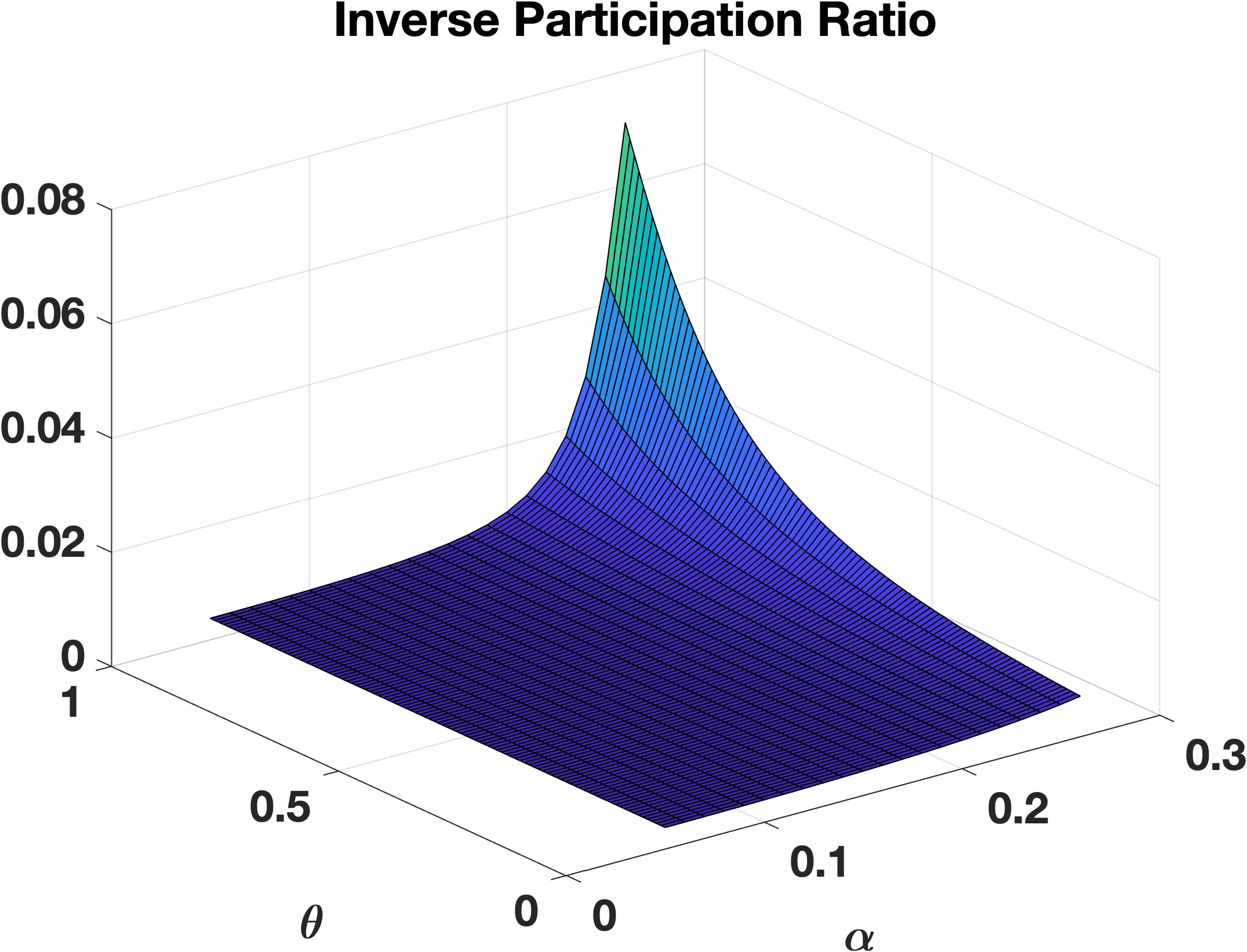
To be concrete, we will quantify localization in terms of the inverse participation ratio, $S(n)$. Here, for a family of unit-norm vectors of increasing dimension, that is, $\mathbf{v}\in\mathbb{R}^{n}$, with $\|\mathbf{v}\|_{2}=1$, letting

$$S(n)=\sum_{i=1}^{n}v_{i}^{4},$$

we say the sequence is localized if $S(n)=O(1)$ as $n\to\infty$ [13]. In the tests below, where $n$ is fixed, we use the size of $S(n)$ as a measure of localization when comparing results, with a larger inverse participation ratio indicating greater localization.

In Figure 4 we show how the inverse participation ratio for the BTDW Katz centrality measure (17) varies as a function of $\theta$ and $\alpha$. For this network, $\rho(A)\approx 3.78$, so standard Katz, that is $\theta=0$, requires $\alpha<1/\rho(A):=\alpha^{\star}\approx 0.264$. In the figure, we use $\alpha$ values of $0.05$, $0.06$, …, $0.26$. We see from the figure that the measure dramatically increases in localization in the regime where backtracking is not suppressed ($\theta\approx 1$) and we are close to an eigenvector measure ($\alpha\approx\alpha^{\star}$). For Figure 5 we made use of independent data from [8] that records the annual passenger usage at each station. We took data for the most recent year, 2017. The idea now is to regard passenger usage (the total number exiting or entering a station) as an indication of importance, and to check whether this correlates with the centrality measure, which is computed only from information about the network structure. We used Kendall’s tau coefficient to quantify the correlation between passenger usage and centrality. (Spearman’s rank correlation coefficient, which is also widely used for assessing rankings, gave similar results.) We see that the most localized regime according to Figure 4 is also the regime with the best correlation coefficient. However, by varying the backtrack-downweighting parameter, $\theta$, it is possible to achieve a reduction in localization. Varying the Katz parameter, $\alpha$, instead, gives a more rapid loss of correlation.

Figure 4: Inverse participation ratio for BTDW Katz centrality on the London Underground transport data.

Figure 5: Kendall’s tau coefficient for BTDW Katz centrality and annual passenger usage on the London Underground transport data.

9 Discussion

Our aim in this work was to define and study a framework that interpolates between traditional and nonbacktracking walk-counting combinatorics. From a network science perspective, this has the potential to combine the benefits of both worlds—notably, avoiding localization while accounting for tree-like structures. Our results also extend theoretical developments in nonbacktracking walks and zeta functions on graphs from a range of related fields [1, 16, 17, 33, 35, 40]. We developed a general four term recurrence in Theorem 3.1 and an expression for the associated generating function in Theorem 4.1. In particular, we showed in Corollary 4.2 that the corresponding Katz-like centrality measure may be computed at the same cost as standard Katz. By considering the relevant limit, Theorem 6.3 then produced an eigenvector centrality measure that interpolates between the traditional and nonbacktracking extremes,

There is considerable scope for further work on backtrack-downweighted walks. In Remark 6.2 we quoted a counterintuitive result on the radius of convergence for the associated generating function on a star graph. This raises questions such as how best to characterize the radius of convergence in general, and under what circumstances the lower bound in Theorem 6.1 is sharp. We are currently studying these issues with the tools of matrix polynomial theory. From the perspective of algorithm design, development of further insights and guidelines concerning the behaviour of backtrack-downweighted Katz in terms of the parameters $\alpha$ and $\theta$ is also of interest.

Acknowledgements The work of FA was supported by fellowship ECF-2018-453 from the Leverhulme Trust. The work of DJH was supported by EPSRC Programme Grant EP/P020720/1. The work of VN was supported by an Academy of Finland grant (Suomen Akatemian päätös 331240).

Appendix A Star Graph Results

Proof of Theorem 5.2

The expressions for $q_{k}(A)$ for $k=0,1,2$ are independent of the structure of the network; they follow immediately from Theorem 3.1.

The adjacency matrix has the form

$$A=\begin{bmatrix}0&\mathbf{1}^{T}\\ \mathbf{1}&\\ \end{bmatrix}.$$

• Let $V=\{1,2,\ldots,m,m+1\}$ be the set of nodes in $S_{1,m}$. The graph is bipartite with node partitions $V_{1}=\{1\}$ and $V_{2}=\{2,\ldots,m+1\}$. It follows that all walks of odd length have to originate from a node in $V_{i}$ and terminate in a node in $V_{j}$, for $i,j=1,2$ and $i\neq j$. This immediately implies that, for all $k=0,1,\ldots$, the matrices $q_{2k+1}(A)$ have the same sparsity pattern as the matrix $A$:

  $$q_{2k+1}(A)=\begin{bmatrix}0&\beta\mathbf{1}^{T}\\ \beta\mathbf{1}^{T}&\end{bmatrix}$$

  for some $\beta>0$.

  We now proceed by induction. When $k=0$ we have that $q_{2k+1}(A)=A=\eta^{k}A$. Suppose now that the result holds for all $\ell\leq k$. We want to show that

  $$q_{2k+3}(A)=\eta^{k+1}A=[\theta(\theta+m-1)]^{k+1}A.$$

  We proceed entrywise by considering the walks of length $2k+3$ from node $1$ to node $i\neq 1$; These are of two types:

  • First type:

    $$\underbrace{1\,\star\,\star\,\cdots\,1\,i}_{(2k+1)\checkmark}\,1\,i,$$

    of which there are $\eta^{k}\theta\theta=\eta^{k}\theta^{2}$. The multiplication by $\theta^{2}$ is used to account for the two backtracking steps introduced when moving from node $i$ to node $i$ in two steps.

  • Second type:

    $$\underbrace{1\,\star\,\star\,\cdots\,1\,j}_{(2k+1)\checkmark}\,1\,i,$$

    for $j\neq i$. Of these there are $\eta^{k}\theta(m-1)$. The multiplication by $(m-1)$ accounts for all the possible choices of $k$, while the multiplication by $\theta$ accounts for the added backtracking steps.

  Overall, by summing these two contributions, it follows that $(q_{2k+3}(A))_{1i}=\eta^{k}(\theta^{2}+\theta(m-1))=\eta^{k+1}$, which concludes this part of the proof.

• Let $k\geq 2$, then from Theorem 3.1

  $$q_{2k}(A) =q_{2k-1}(A)A+(1-\theta)q_{2(k-1)}(A)B$$

  $$=\eta^{k-1}A^{2}+(1-\theta)[q_{2k-3}(A)A+(1-\theta)q_{2(k-2)}(A)B]B$$

  $$=\eta^{k-1}A^{2}+(1-\theta)\eta^{k-2}A^{2}B+(1-\theta)^{2}q_{2(k-2)}(A)B^{2}$$

  $$=A^{2}\sum_{j=0}^{k-3}\eta^{k-1-j}((1-\theta)B)^{j}+(1-\theta)^{k-2}[q_{3}(A)A+(1-\theta)q_{2}(A)B]B^{k-2}$$

  $$=A^{2}\sum_{j=0}^{k-1}\eta^{k-1-j}((1-\theta)B)^{j}-(1-\theta)^{k}DB^{k-1}$$

  $$=\eta^{k-1}A^{2}\left(I-\left(\frac{1-\theta}{\eta}B\right)^{k}\right)\left(I-\frac{1-\theta}{\eta}B\right)^{-1}-(1-\theta)^{k}DB^{k-1},$$

  where we have used the fact that

  $$B=(1-\theta)I-D=-\begin{bmatrix}\theta+m-1&\\ &\theta I\\ \end{bmatrix}$$

  and hence the matrix $I-\frac{1-\theta}{\eta}B$ is invertible.

Proof of Corollary 5.3

Corollary 5.3 now follows after inserting the expressions for $q_{k}(A)$ in Theorem 5.2 into (16) and simplifying, for all $\theta\in(0,1]$. When $\theta=0$, i.e., in the fully nonbacktracking setting, the result follows from a direct computation, since the length of the longest possible nonbacktracking walk in $S_{1,m}$ is two:

$$x_{1}=1+\alpha m,\quad\text{ and }\quad x_{i}=1+\alpha+\alpha^{2}(m-1)$$

for all $i=2,\ldots,m+1$.

References

- [1] O. Angel, J. Friedman, and S. Hoory, The non-backtracking spectrum of the universal cover of a graph, Transactions of the American Mathematical Society, 326 (2015), pp. 4287–4318.
- [2] F. Arrigo, P. Grindrod, D. J. Higham, and V. Noferini, Non-backtracking walk centrality for directed networks, Journal of Complex Networks, 6 (2018), pp. 54–78.
- [3] , On the exponential generating function for non-backtracking walks, Linear Algebra and Its Applications, 79 (2018), pp. 781–801.
- [4] M. Benzi and C. Klymko, Total communicability as a centrality measure, Journal of Complex Networks, 1 (2013), pp. 124–149.
- [5] M. Benzi and C. Klymko, On the limiting behavior of parameter-dependent network centrality measures, SIAM J. Matrix Anal. Appl., 36 (2015), pp. 686–706.
- [6] P. Boldi and S. Vigna, Axioms for centrality, Internet Mathematics, 10 (2014), pp. 222–262.
- [7] R. Bowen and O. E. Lanford, Zeta functions of restrictions of the shift transformation, in Global Analysis: Proceedings of the Symposium in Pure Mathematics of the Americal Mathematical Society, University of California, Berkely, 1968, S.-S. Chern and S. Smale, eds., American Mathematical Society, 1970, pp. 43–49.
- [8] S. Cipolla, F. Durastante, and F. Tudisco, Nonlocal PageRank, ESIAM, to appear, (2020).
- [9] R. Criado, J. Flores, E. García, A. J. G. del Amo, À. Pérez, and M. Romance, On the alpha-nonbacktracking centrality for complex networks: Existence and limit cases, Journal of Computational and Applied Mathematics, 350 (2019), pp. 35–45.
- [10] M. De Domenico, A. Solé-Ribalta, S. Gómez, and A. Arenas, Navigability of interconnected networks under random failures, Proceedings of the National Academy of Sciences, 111 (2014), pp. 8351–8356.
- [11] E. Estrada and D. J. Higham, Network properties revealed through matrix functions, SIAM Review, 52 (2010), pp. 696–671.
- [12] L. C. Freeman, Centrality in social networks conceptual clarification, Social Networks, 1 (1978), pp. 215–239.
- [13] A. V. Goltsev, S. N. Dorogovtsev, J. G. Oliveira, and J. F. F. Mendes, Localization and spreading of diseases in complex networks, Phys. Rev. Lett., 109 (2012), p. 128702.
- [14] P. Grindrod, D. J. Higham, and V. Noferini, The deformed graph Laplacian and its applications to network centrality analysis, SIAM Journal on Matrix Analysis and Applications, 39 (2018), pp. 310–341.
- [15] R. A. Horn and C. R. Johnson, Matrix Analysis, Cambridge University Press, Cambridge, 1985.
- [16] M. D. Horton, Ihara zeta functions on digraphs, Linear Algebra and its Applications, 425 (2007), pp. 130–142.
- [17] M. D. Horton, H. M. Stark, and A. A. Terras, What are zeta functions of graphs and what are they good for?, in Quantum graphs and their applications, G. Berkolaiko, R. Carlson, S. A. Fulling, and P. Kuchment, eds., vol. 415 of Contemp. Math., 2006, pp. 173–190.
- [18] L. Katz, A new index derived from sociometric data analysis, Psychometrika, 18 (1953), pp. 39–43.
- [19] T. Kawamoto, Localized eigenvectors of the non-backtracking matrix, Journal of Statistical Mechanics: Theory and Experiment, 2016 (2016), p. 023404.
- [20] P. A. Knight and E. Estrada, A First Course in Network Theory, Oxford University Press, Oxford, 2015.
- [21] F. Krzakala, C. Moore, E. Mossel, J. Neeman, A. Sly, L. Zdeborová, and P. Zhang, Spectral redemption: clustering sparse networks, Proceedings of the National Academy of Sciences, 110 (2013), pp. 20935–20940.
- [22] T. Martin, X. Zhang, and M. E. J. Newman, Localization and centrality in networks, Phys. Rev. E, 90 (2014), p. 052808.
- [23] P.-A. G. Maugis, S. C. Olhede, and P. J. Wolfe, Topology reveals universal features for network comparison, arXiv:1705.05677 [stat.ME], (2017).
- [24] S. Moore and T. Rogers, Predicting the speed of epidemics spreading in networks, Phys. Rev. Lett., 124 (2020), p. 068301.
- [25] F. Morone and H. A. Makse, Influence maximization in complex networks through optimal percolation, Nature, 524 (2015), pp. 65–68.
- [26] F. Morone, B. Min, L. Bo, R. Mari, and H. A. Makse, Collective influence algorithm to find influencers via optimal percolation in massively large social media, Scientific Reports, 6 (2016), p. 30062.
- [27] M. E. J. Newman, Networks: an Introduction, Oxford Univerity Press, Oxford, 2010.
- [28] , Spectral community detection in sparse networks, arXiv:1308.6494, (2013).
- [29] R. Pastor-Satorras and C. Castellano, Distinct types of eigenvector localization in networks, Scientific Reports, 6 (2016), p. 18847.
- [30] K. Polovnikov, A. Gorsky, S. Nechaev, S. V. Razin, and S. V. Ulianov, Non-backtracking walks reveal compartments in sparse chromatin interaction networks, Scientific Reports, 10 (2020).
- [31] A. Saade, F. Krzakala, and L. Zdeborová, Spectral clustering of graphs with the Bethe Hessian, in Advances in Neural Information Processing Systems 27, Z. Ghahramani, M. Welling, C. Cortes, N. D. Lawrence, and K. Q. Weinberger, eds., 2014, pp. 406–414.
- [32] A. Singh and M. D. Humphries, Finding communities in sparse networks, Scientific Reports, 5 (2015).
- [33] U. Smilansky, Quantum chaos on discrete graphs, Journal of Physics A: Mathematical and Theoretical, 40 (2007), p. F621.
- [34] S. Sodin, Random matrices, non-backtracking walks, and the orthogonal polynomials, J. Math. Phys, 48 (2007), p. 123503.
- [35] H. Stark and A. Terras, Zeta functions of finite graphs and coverings, Advances in Mathematics, 121 (1996), pp. 124–165.
- [36] A. Tarfulea and R. Perlis, An Ihara formula for partially directed graphs, Linear Algebra and its Applications, 431 (2009), pp. 73–85.
- [37] A. Terras, Harmonic Analysis on Symmetric Spaces — Euclidean Space, the Sphere, and the Poincaré Upper Half-Plane, Springer, New York, 2nd ed., 2013.
- [38] L. Torres, K. S. Chan, H. Tong, and T. Eliassi-Rad, Node immunization with non-backtracking eigenvalues, tech. rep., arXiv:2002.12309, 2020.
- [39] L. Torres, P. Suárez-Serrato, and T. Eliassi-Rad, Non-backtracking cycles: Length spectrum theory and graph mining applications, Journal of Applied Network Science, 4 (2019).
- [40] Y. Watanabe and K. Fukumizu, Graph zeta function in the Bethe free energy and loopy belief propagation, in Advances in Neural Information Processing Systems 22, Y. Bengio, D. Schuurmans, J. Lafferty, C. Williams, and A. Culotta, eds., 2009, pp. 2017–2025.