Explicit geometric construction of sparse inverse mass matrices for arbitrary tetrahedral grids

Abstract

The geometric reinterpretation of the Finite Element Method (FEM) shows that Raviart–Thomas and Nédélec mass matrices map from degrees of freedoms (DoFs) attached to geometric elements of a tetrahedral grid to DoFs attached to the barycentric dual grid. The algebraic inverses of the mass matrices map DoFs attached to the barycentric dual grid back to DoFs attached to the corresponding primal tetrahedral grid, but they are of limited practical use since they are dense.

In this paper we present a new geometric construction of sparse inverse mass matrices for arbitrary tetrahedral grids and possibly anisotropic materials, debunking the conventional wisdom that the barycentric dual grid prohibits a sparse representation for inverse mass matrices. In particular, we provide a unified framework for the construction of both edge and face mass matrices and their sparse inverses. Such a unifying principle relies on novel geometric reconstruction formulas, from which, according to a well-established design strategy, local mass matrices are constructed as the sum of a consistent and a stabilization term. A major difference with the approaches proposed so far is that the consistent term is defined geometrically and explicitly, that is, without the necessity of computing the inverses of local matrices. This provides a sensible speedup and an easier implementation. We use these new sparse inverse mass matrices to discretize a three-dimensional Poisson problem, providing the comparison between the results obtained by various formulations on a benchmark problem with analytical solution.

1 Introduction

Many physics-compatible discretization methods depend on a primal-dual mesh structure and the related staggered positioning of the physical variables [1], often referred to as degrees of freedom (DoFs). In particular, most physics-compatible discretizations for the Maxwell’s equations introduced so far, like the Yee-scheme [2], the Cell Method (CM) [1], [3], the Finite Integration Technique [4], the Discrete Geometric Approach (DGA) [5], [6], the Compatible Discrete Operators (CDO) [7] are based on a pair of interlocked primal and dual grids. In other physics-compatible methods like the Mimetic Finite Difference method [8] and the Finite Element Method (FEM) based on Whitney edge and face basis functions (i.e. the Nédélec curl-conforming basis functions and the Raviart–Thomas div-conforming basis functions) [9], [10], a dual grid is not explicitly used but an interpretation using it is readily available [11], [10], at least for the lowest order version.

A fundamental principle of compatible numerical schemes is the distinction between topological equations and constitutive equations [1], [12]. Topological equations express conservation laws of physical theories. As the name suggests, topological equations are valid under arbitrary homeomorphic transformations of the domain in which they are defined. Constitutive equations, also called material equations, describe the behaviour of material, substance or medium under interest. The discrete Hodge star operator [13], [10] acts as discrete counterpart of the material parameters used to formulate constitutive equations and its form depends on the analytic form of the material parameters and on the geometric properties of the grid which discretizes the computational domain. In particular, the algebraic realization of the Hodge operator is given by the so-called mass matrices [11], [13], [10].

What is usually achieved is the construction of discrete Hodge operators which map DoFs attached to primal faces to DoFs attached to dual edges or DoFs attached to primal edges to DoFs attached to dual faces [13], [10], [5], [6]. This is exactly what the FEM mass matrices computed with Raviart–Thomas and Nédélec basis functions perform, [11], [10], respectively.

However, we can nonetheless define inverse discrete Hodge operators that map DoFs attached to dual geometric elements to DoFs attached to primal geometric elements. Explicitly computing the algebraic inverse of the mass matrix is not considered a viable solution given that such a matrix would be dense, so of questionable usefulness in practice. Therefore, we are in particular interested in a sparse realization of inverse discrete Hodge operators. Inverse Hodge operators play a vital role in many applications. Most notably, inverse Hodge operators enable consistent and explicit schemes to solve time-domain wave propagation problems [2], [14], [15], [16]. Other applications enabled by the inverse mass matrices comprise the explicit construction of the codifferential operator, the Laplace–de Rham operator [17] and compute the discrete Hodge decomposition of discrete fields [17], [18].

The construction of inverse Hodge operators for tetrahedral grids is not entirely new. In CM [1], [3], Discrete Exterior Calculus (DEC) [19] and in the cell-centered Finite Volume literature [20], a Voronoï dual grid based on circumcenters is used, and the resulting mass matrices are diagonal in such a way that their inverses can be easily computed. It is important to note that, when the material is anisotripic, the mass matrices are in general not diagonal, so a sparse inverse Hodge operator cannot be easily constructed. Another solution using a Voronoï dual grid is presented in [21]. However, most commonly used mesh generators like NETGEN and GMSH produce tetrahedral grids that are not Delaunay and in this case the Voronoï dual grid cannot be defined [22].

The aim of this paper is to extend the construction of sparse inverse Hodge operators on barycentric dual grids which can be defined for arbitrary tetrahedral grids. The barycentric dual grids are explicitly used in DGA [6] and implicitly in the Finite Element Method (FEM) [11] and in the MFD [8]. Yet, devising a recipe to construct sparse inverse Hodge operators on a barycentric dual grid appears to be a formidable task [23], [15], [17], [21] given that the conventional wisdom is that the barycentric dual grid “prohibits a sparse representation for their inverse operators” [24] and, consequently, only approximate constructions have been proposed [15].

By using a barycentric dual grid, in [14], [16], inverse mass matrices that map from dual faces to primal edges are constructed by assembling local contributions inside dual cells and then computing the algebraic inverse of the resulting local matrices. Yet, we note that the time needed to compute all local inverses is not negligible, because the rank of the local matrices is twenty or more.

In this paper we provide a unified framework for the construction of both edge and face mass matrices and their sparse inverses. The unifying principle relies on the construction of discrete Hodge operators starting from reconstruction formulas (that provide a representation of the discrete variables at the continuous level) defined by geometric elements of primal and dual grids. Starting from these reconstruction formulas, local mass matrix is constructed according to a well-established design strategy, as the sum of a consistent and a stabilization term [8], [25]. While the consistent term is fixed, the stabilization term depends on some user-dependent parameters, which for instance, offer the possibility of controlling the eingenvalues of the matrices.

The construction of the inverse mass matrix that maps from dual edges of a barycentric dual grid to primal faces of a tetrahedral grid proposed in this paper is entirely new. A key difference with respect to the approach proposed in [14],[16] in the construction of the other inverse mass matrix that maps from dual faces of the barycentric dual grid to primal edges of the simplicial grid is the explicit and geometric construction of the consistent term, without the necessity of computing local inverses. In addition, the recipe to construct the stabilization term adds more flexibility in the construction of the mass matrices.

In general, the major contribution of our construction is not only to have avoided the computation of the local inverses, but rather the fact that it results in symmetric expressions for both types of local mass matrices, thus highlighting the duality relationship between the pair of grids. A key requirement of our setting turns out to be that the material parameters are constant on dual cells associated with the nodes of the primal simplicial grid. To deal with the general case of material parameters that are constant on the grid cells, but arbitrary discontinuous across the interfaces between the cells, two different approaches are proposed. The first one is a weighted averaging technique classically used in Finite Volumes Methods [20]. The second one is based on an extension of the approach proposed [14],[16].

The paper is organized as follows. In Section 2, we introduce the geometric elements from which general tetrahedral grids and their barycentric dual are constructed. In addition, we present the basic building blocks of low-order compatible numerical schemes that will be used in the work. In Section 3, we detail the construction of mass matrices. In Section 4, following the same design principles of the previous section, we detail the construction of inverses of mass matrices. In addition, we describe how to deal with problems having inhomogeneous materials. In Section 5, we present an application of the newly derived inverse mass matrices to a Poisson problem and we provide a comparison among different formulations that can be used to solve the same problem on the same mesh. Finally, in Section 6, the conclusions are drawn.

2 Compatible discretization

A detailed presentation of compatible discretizations can be found in [26]. In what follows, we only present the main ideas that will be used throughout the paper.

2.1 Geometry of primal and dual grid

Let us consider a subdivision of a region $\Omega$ of $\mathbb{R}^{3}$ into a primal tetrahedral grid $K=(N,E,F,C)$, where the sets $N,E,F$ and $C$ contain the grid nodes, edges, faces and cells (or tetrahedra), respectively. We denote a single node as $n$, an edge by $e$, a face by $f$ and a cell by $c$, respectively, see Fig. 1. The geometric elements of the primal grid are provided with an inner orientation [1], [12].

Figure 1: Primal and dual geometric elements of a tetrahedron $c\in C$. (a) Dual cell. (b) Dual face. (c) Dual edge.

Let $X$ be any set among $N,E,F,$ or $C$. If $r$ is a geometric element of $K$, we denote by $X(r)$ the subset defined by

$$X(r)\coloneqq\{x\in X\mid r\subset x\},$$ (1)

if Eq. 1 is not void, or otherwise,

$$X(r)\coloneqq\{x\in X\mid x\subset r\}.$$ (2)

For instance, $C(e)=\{c\in C\mid e\subset c\}$ is the cluster of cells of $C$ that contain the edge $e$ and $E(c)=\{e\in E\mid e\subset c\}$ collects the edges of $c\in C$.

Interlocked with the primal grid $K$, a barycentric dual grid [27], [1], [12] $\tilde{K}=(\tilde{N},\tilde{E},\tilde{F},\tilde{C})$ is introduced, where the sets $\tilde{N},\tilde{E},\tilde{F}$ and $\tilde{C}$ contain dual nodes, dual edges, dual faces and dual cells, respectively. Each geometric entity of the dual grid is in one-to-one correspondence (duality pairing) with a geometric element of the primal grid and it is constructed by means of the barycentric subdivision [27] of the primal grid, see Fig. 1. With symbol “$\mathtt{\sim}$” we denote geometric elements of the dual grid, thus, we denote a single dual node as $\tilde{n}$, a dual edge by $\tilde{e}$, a dual face by $\tilde{f}$ and a dual cell by ${\tilde{c}}$, respectively. With a subscript we indicate the corresponding (unique) geometric element of the primal grid, thus, the dual of a primal node $n$ is a dual cell ${\tilde{c}}_{n}$, the dual of a primal edge $e$ is a dual face $\tilde{f}_{e}$, the dual of a primal face $f$ is a dual edge $\tilde{e}_{f}$ and the dual of a primal cell $c$ is the dual node denoted as $\tilde{n}_{c}$.

To describe the geometric elements of the pair of grids, we introduce a Cartesian system of coordinates with specified origin and we denote by $\bm{x}=(x_{1},x_{2},x_{3})^{T}$ the coordinates of its generic point. Let us first describe the construction of the restriction of dual geometric elements to a single cell $c$, as the one pictured in Fig. 1. The geometric construction of the dual nodes, dual edges, dual faces and dual cells is based on the barycentric subdivision as follows. To begin with, let us define the barycenters of geometric elements. The barycenters of an edge $e$, face $f$ and of a cell $c$ are defined, respectively, as follows

$$\bm{b}_{e}=\frac{1}{|{e}|}\int_{e}\bm{x}\,dl\,, \bm{b}_{f}=\frac{1}{|{f}|}\int_{f}\bm{x}\,dS\,, \bm{b}_{c}=\frac{1}{|{c}|}\int_{c}\bm{x}\,dV\,,$$ (3)

where $|{e}|,|{f}|$ and $|{c}|$ denote the length of edge $e$, the area of face $f$ and the volume of cell $c$, respectively.

A dual node $\tilde{\bm{n}}_{c}$ is the barycenter $\bm{b}_{c}$ of $c$. A dual edge ${{}\tilde{e}_{f}}_{\mkern 1.0mu\vrule height=3.01389pt\mkern 2.0muc}$ is a segment which joins $\tilde{\bm{n}}_{c}$ with the barycenter $\bm{b}_{f}$ of a primal face $f$. A dual face ${{}\tilde{f}_{e}}_{\mkern 1.0mu\vrule height=3.01389pt\mkern 2.0muc}$ is a quadrilateral plane surface whose vertices are $\tilde{\bm{n}}$, the barycenters of the pair of primal faces having a primal edge $e$ in common and the barycenter $\bm{b}_{e}$ of $e$. A dual cell ${{}{\tilde{c}}_{n}}_{\mkern 1.0mu\vrule height=3.01389pt\mkern 2.0muc}$ is a region whose boundary is made of a disjoint union of dual faces, corresponding to edges of $c$ having the node $n$ in common, and portions of faces of $c$ having the node $n$ in common. Dual edge $\tilde{e}_{f}$, dual face $\tilde{f}_{e}$ and dual cell ${\tilde{c}}_{n}$ are endowed with outer orientation [1], [12], in such a way that each of the pairs $(e,\tilde{f}_{e}),(f,\tilde{e}_{f}),(n,{\tilde{c}}_{n})$ are oriented according to the right-hand rule.

To each of the following geometric elements $e,f,{{}\tilde{f}}_{\mkern 1.0mu\vrule height=3.01389pt\mkern 2.0muc},{{}\tilde{e}}_{\mkern 1.0mu\vrule height=3.01389pt\mkern 2.0muc}$ of the primal or of the dual grid, we associate their corresponding vectors $\bm{e},\bm{f},{{}\tilde{\bm{f}}}_{\mkern 1.0mu\vrule height=3.01389pt\mkern 2.0muc},{{}\tilde{\bm{e}}}_{\mkern 1.0mu\vrule height=3.01389pt\mkern 2.0muc}$ respectively. Each of these vectors, will be represented with a column array of its cartesian components. Vector $\bm{e}$ is the edge vector associated with edge $e$; for example $\bm{e}=(e_{1},e_{2},e_{3})^{T}=\bm{n}_{i}-\bm{n}_{j},i\neq j$, where $\bm{n}_{i}$ and $\bm{n}_{j}$ are the coordinates of the boundary nodes of $\bm{e}$. $\bm{t}_{e}$ represents the unit vector parallel to and oriented as $\bm{e}$ in such a way that $\bm{e}=|{e}|\bm{t}_{e}$. Vector $\bm{f}$ is the face vector associated with face $f$ defined as $\bm{f}=|{f}|\bm{n}_{f}$, where $\bm{n}_{f}$ is the unit vector normal to and oriented as $f$. In a similar way, vector ${{}\tilde{\bm{e}}_{f}}_{\mkern 1.0mu\vrule height=3.01389pt\mkern 2.0muc}$ is the edge vector associated with the dual edge ${{}\tilde{e}_{f}}_{\mkern 1.0mu\vrule height=3.01389pt\mkern 2.0muc}$; for instance, ${{}\tilde{\bm{e}}_{f}}_{\mkern 1.0mu\vrule height=3.01389pt\mkern 2.0muc}=\bm{b}_{f}-\tilde{\bm{n}}_{c}$, see Fig. 1b. Vector ${{}\tilde{\bm{f}}_{e}}_{\mkern 1.0mu\vrule height=3.01389pt\mkern 2.0muc}$ is the face vector associated with the dual face ${{}\tilde{f}_{e}}_{\mkern 1.0mu\vrule height=3.01389pt\mkern 2.0muc}$. Face vector ${{}\tilde{\bm{f}}_{e}}_{\mkern 1.0mu\vrule height=3.01389pt\mkern 2.0muc}$ is equal to ${{}\tilde{\bm{f}}_{e}}_{\mkern 1.0mu\vrule height=3.01389pt\mkern 2.0muc}=\frac{1}{2}\big({{}\tilde{\bm{e}}_{f_{i}}}_{\mkern 1.0mu\vrule height=3.01389pt\mkern 2.0muc}\times(\bm{b}_{e}-\tilde{\bm{n}}_{c})-{{}\tilde{\bm{e}}_{f_{j}}}_{\mkern 1.0mu\vrule height=3.01389pt\mkern 2.0muc}\times(\bm{b}_{e}-\tilde{\bm{n}}_{c})\big)$ with $f_{i},f_{j}$ two faces such that $e=f_{i}\cap f_{j}$, with $i=i(e)$ and $j=j(e)$, and in such a way that the expression induces the correct orientation on ${{}\tilde{\bm{f}}_{e}}_{\mkern 1.0mu\vrule height=3.01389pt\mkern 2.0muc}$, see Fig. 1b.

Now, starting from the definition of dual geometric elements restricted to a single cell $c$, we introduce dual edges, dual faces and dual cells of the barycentric dual grid. We define a dual edge $\tilde{e}_{f}$ as the piecewise segment made of the union of the two segments ${{}\tilde{e}_{f}}_{\mkern 1.0mu\vrule height=3.01389pt\mkern 2.0muc_{1}}$ and ${{}\tilde{e}_{f}}_{\mkern 1.0mu\vrule height=3.01389pt\mkern 2.0muc_{2}}$, with $c_{1},c_{2}\in C(f)$. The corresponding vector $\tilde{\bm{e}}_{f}$ is defined as follows $\tilde{\bm{e}}_{f}\coloneqq\sum_{c\in C(f)}{{}\tilde{\bm{e}}_{f}}_{\mkern 1.0mu\vrule height=3.01389pt\mkern 2.0muc}$. A dual face $\tilde{f}_{e}$ is defined as the polyhedral surface made of the union of all ${{}\tilde{f}_{e}}_{\mkern 1.0mu\vrule height=3.01389pt\mkern 2.0muc}$, with $c\in C(e)$. The corresponding dual face vector $\tilde{\bm{f}}_{e}$ is defined as follows $\tilde{\bm{f}}_{e}\coloneqq\sum_{c\in C(e)}{{}\tilde{\bm{f}}_{e}}_{\mkern 1.0mu\vrule height=3.01389pt\mkern 2.0muc}$. A dual cell ${\tilde{c}}_{n}$ is defined as the region made of the union of all ${{}{\tilde{c}}_{n}}_{\mkern 1.0mu\vrule height=3.01389pt\mkern 2.0muc}$, with $c\in C(n)$, that is ${\tilde{c}}_{n}\coloneqq\bigcup_{c\in C(n)}{{}{\tilde{c}}_{n}}_{\mkern 1.0mu\vrule height=3.01389pt\mkern 2.0muc}$. Note that the boundary of each dual cell decomposes into dual edges and dual faces.

Let $X$ be any set among $E,F$ and let $\tilde{X}$ be any set among $\tilde{E},\tilde{F}$. Given a non-empty region $\Omega^{\prime}\subset\Omega$ of $\mathbb{R}^{3}$, we define

$${{}X}_{\mkern 1.0mu\vrule height=3.01389pt\mkern 2.0mu\Omega^{\prime}}\coloneqq\{x\cap\Omega^{\prime},x\in X\}, {{}\tilde{X}}_{\mkern 1.0mu\vrule height=3.01389pt\mkern 2.0mu\Omega^{\prime}}\coloneqq\{\tilde{x}\cap\Omega^{\prime},\tilde{x}\in X\},$$ (4)

as the subsets of geometric elements of $X$ and $\tilde{X}$ restricted to $\Omega^{\prime}$, respectively. In the sequel we consider the cases where $\Omega^{\prime}$ is one among a cell $c\in C$, a dual cell ${\tilde{c}}\in\tilde{C}$, or the restriction of the dual cell ${\tilde{c}}$ to the cell $c$, ${{}{\tilde{c}}}_{\mkern 1.0mu\vrule height=3.01389pt\mkern 2.0muc}$. As an instance, $E_{\mkern 1.0mu\vrule height=3.01389pt\mkern 2.0mu{\tilde{c}}}:=\{e\cap{\tilde{c}},e\in E\}$ contains the restriction of primal edges to the dual cell ${\tilde{c}}$. Observe that $E_{\mkern 1.0mu\vrule height=3.01389pt\mkern 2.0muc},F_{\mkern 1.0mu\vrule height=3.01389pt\mkern 2.0muc}$ coincide with the subsets of all edges and faces of $c$. Similarly, $\tilde{E}_{\mkern 1.0mu\vrule height=3.01389pt\mkern 2.0mu{\tilde{c}}},\tilde{F}_{\mkern 1.0mu\vrule height=3.01389pt\mkern 2.0mu{\tilde{c}}}$ coincide with the subsets of all dual edges and dual faces of ${\tilde{c}}$. Since dual cells are constructed according to the barycentric subdivision, the length of each edge $e^{\prime}\in E_{\mkern 1.0mu\vrule height=3.01389pt\mkern 2.0mu{\tilde{c}}}$ is half of the length of a primal edge. Moreover, the area of each face $f^{\prime}\in F_{\mkern 1.0mu\vrule height=3.01389pt\mkern 2.0mu{\tilde{c}}}$ is a third of the area of a primal face [28].

Finally, we introduce the corresponding matrices ${{}\mathbb{X}}_{\mkern 1.0mu\vrule height=3.01389pt\mkern 2.0mu\Omega^{\prime}},{{}\tilde{\mathbb{X}}}_{\mkern 1.0mu\vrule height=3.01389pt\mkern 2.0mu\Omega^{\prime}}$ whose rows collect geometric vectors associated with elements of the sets in Eq. 4. As an instance, rows of $\mathbb{E}_{\mkern 1.0mu\vrule height=3.01389pt\mkern 2.0mu{\tilde{c}}}$ contain edge vectors associated with edges in $E_{\mkern 1.0mu\vrule height=3.01389pt\mkern 2.0mu{\tilde{c}}}$.

2.2 Degrees of Freedom and reconstruction operators

The physical variables, often referred to as degrees of freedom (DoFs), involved in a discrete formulation of a computational problem, have a precise association with the geometric elements of the pair of staggered primal-dual grids [1], [12]. DoFs are obtained by evaluating the physical vector fields on the geometric elements of the grid, and are collected in finite dimensional arrays of real numbers endowed with a natural vector space structure. The operation of translating a vector field into the corresponding DoFs is performed by means of integration using the so-called de Rham maps [13], [10]. We focus on DoFs attached to edges and faces of the primal and dual grid. We denote the vector space of edge DoFs, face DoFs, dual edge DoFs and dual face DoFs by $\mathcal{E}$, $\mathcal{F}$, ${\tilde{\mathcal{E}}}$, and ${\tilde{\mathcal{F}}}$, respectively. Given a vector field $\bm{u}$, we denote with ${\bm{u}}^{\,\mathcal{E}}$, ${\bm{u}}^{\,\mathcal{F}}$, ${\bm{u}}^{\,{\tilde{\mathcal{E}}}}$, and ${\bm{u}}^{\,{\tilde{\mathcal{F}}}}$ the DoFs of $\bm{u}$ in $\mathcal{E}$, $\mathcal{F}$, ${\tilde{\mathcal{E}}}$, and ${\tilde{\mathcal{F}}}$, respectively.

We introduce the following specialized definitions of the de Rham maps, which follows as a special case of the general definition applied to the vector subspace of constant vector fields.

Let us consider a constant vector field $\bm{u}$. Given a non-empty region $\Omega^{\prime}\subset\Omega$, we define the corresponding subset of DoFs of $\bm{u}$ restricted to the region $\Omega^{\prime}$ as follows

$${\bm{u}}^{\mathcal{E}}_{\mkern 1.0mu\vrule height=3.01389pt\mkern 2.0mu\Omega^{\prime}}=\mathbb{E}_{\mkern 1.0mu\vrule height=3.01389pt\mkern 2.0mu\Omega^{\prime}}\bm{u},\;{\bm{u}}^{\mathcal{F}}_{\mkern 1.0mu\vrule height=3.01389pt\mkern 2.0mu\Omega^{\prime}}=\mathbb{F}_{\mkern 1.0mu\vrule height=3.01389pt\mkern 2.0mu\Omega^{\prime}}\bm{u},\;{\bm{u}}^{{\tilde{\mathcal{E}}}}_{\mkern 1.0mu\vrule height=3.01389pt\mkern 2.0mu\Omega^{\prime}}=\tilde{\mathbb{E}}_{\mkern 1.0mu\vrule height=3.01389pt\mkern 2.0mu\Omega^{\prime}}\bm{u},\;{\bm{u}}^{{\tilde{\mathcal{F}}}}_{\mkern 1.0mu\vrule height=3.01389pt\mkern 2.0mu\Omega^{\prime}}=\tilde{\mathbb{F}}_{\mkern 1.0mu\vrule height=3.01389pt\mkern 2.0mu\Omega^{\prime}}\bm{u}.$$ (5)

A reconstruction operator is defined as a formal inverse of the de Rham map restricted to the vector subspace of constant vector fields. Thus, reconstruction operators map DoFs to a constant vector field defined on a cell. In the sequel we will always refer to local reconstruction operators in such a way that the domain of definition of the reconstructed vector field is a given cell.

3 Mass matrices

In compatible numerical methods, it is always necessary to map DoFs attached to geometric elements of the primal grid into DoFs attached to geometric elements of the dual grid, or viceversa [1], [11], [12]. This process of converting one type of DoFs to another is performed by the so-called discrete Hodge star operator [13]. This operator is required to satisfy a set of properties. A first requirement is consistency, which will be specified in the next subsections, and symmetry. In addition, we require positive definiteness, which assures the stability of the resulting numerical scheme.

One possible method for explicitly converting one type of DoFs into another is to reconstruct the polynomial vector field in each cell starting from DoFs attached to a set of geometric elements, and then project this vector field onto the corresponding geometric elements related by duality. We will follow this principle to design both types of local mass matrices, which give a discrete realization of the corresponding discrete Hodge operators.

In this section we show how to construct consistent mass matrices which map DoFs attached to primal geometric elements to DoFs attached to dual geometric elements. Novel proofs are given based on Stokes’ theorem.

3.1 Primal cell reconstruction

Let us consider a pair of vector fields $\bm{u},\bm{w}:\mathbb{R}^{3}\rightarrow\mathbb{R}^{3}$ along with a scalar field $w:\mathbb{R}^{3}\rightarrow\mathbb{R}$ defined on a given cell $c$. The following well-known integration by parts formulas hold

$$\int_{c}\bm{u}\cdot\gradient w\,dV=-\int_{c}\divergence\bm{u}\,w\,dV+\int_{\partial c}\bm{u}\cdot\bm{n}\,w\,dS,$$ (6)

$$\int_{c}\bm{u}\cdot\curl{\bm w}\,dV=\int_{c}\curl\bm{u}\cdot\bm{w}\,dV+\int_{\partial c}\bm{u}\times\bm{n}\cdot\bm{w}\,dS.$$ (7)

Lemma 1 (Reconstruction formulas).

The following tensor identities hold

$$\sum_{f\in F(c)}{{}\tilde{\bm{e}}_{f}}_{\mkern 1.0mu\vrule height=3.01389pt\mkern 2.0muc}\otimes\bm{f}=|{c}|\,\mathbb{I}_{3},$$ (8)

$$\sum_{e\in E(c)}{{}\tilde{\bm{f}}_{e}}_{\mkern 1.0mu\vrule height=3.01389pt\mkern 2.0muc}\otimes\bm{e}=|{c}|\,\mathbb{I}_{3}.$$ (9)

Proof.

Let $\bm{u},\bm{w}\in\mathbb{R}^{3}$. Thanks to Eq. 6, we have

$$\begin{split}|{c}|\,\bm{u}\cdot\bm{w}\,&=\int_{c}\bm{u}\cdot\bm{w}\,dV=\int_{c}\bm{u}\cdot\gradient(\bm w \cdot(\bm x - \bdual n_\C))\,dV\\ &=\int_{\partial c}(\bm{u}\cdot\bm{n})\,(\bm{w}\cdot(\bm{x}-\tilde{\bm{n}}_{c}))\,dS=\sum_{f\in F(c)}(\bm{u}\cdot\bm{f})\,((\bm{b}_{f}-\tilde{\bm{n}}_{c})\cdot\bm{w}).\end{split}$$ (10)

By using the definition of ${{}\tilde{\bm{e}}_{f}}_{\mkern 1.0mu\vrule height=3.01389pt\mkern 2.0muc}$, it follows that

$$|{c}|\,\bm{u}\cdot\bm{w}=\sum_{f\in F(c)}(\bm{u}\cdot\bm{f})\,({{}\tilde{\bm{e}}_{f}}_{\mkern 1.0mu\vrule height=3.01389pt\mkern 2.0muc}\cdot\bm{w}).$$ (11)

Since $\bm{w}$ is arbitrary, Eq. 8 is proved.

Thanks to Eq. 7, we have

$$\begin{split}2|{c}|\,\bm{u}\cdot\bm{w}&=2\int_{c}\bm{u}\cdot\bm{w}\,dV=\int_{c}\bm{u}\cdot\curl\big(\bm w \times(\bm x - \bdual n_\C)\big)\,dV\\ &=\int_{\partial c}(\bm{u}\times\bm{n})\cdot\big(\bm{w}\times(\bm{x}-\tilde{\bm{n}}_{c})\big)\,dS=\sum_{f\in F(c)}\int_{f}(\bm{u}\times\bm{n}_{f})\cdot\big(\bm{w}\times(\bm{x}-\tilde{\bm{n}}_{c})\big)\,dS\\ &=\sum_{f\in F(c)}|{f}|\,(\bm{u}\times\bm{n}_{f})\cdot(\bm{w}\times{{}\tilde{\bm{e}}_{f}}_{\mkern 1.0mu\vrule height=3.01389pt\mkern 2.0muc}).\end{split}$$ (12)

Now, by applying the same argument used in Eq. 10 to the vector $\bm{u}\times\bm{n}_{f}$ restricted to a face $f$, we obtain

$$|{f}|\,\bm{u}\times\bm{n}_{f}=\sum_{e\in E(f)}(\bm{u}\cdot\bm{e})\,(\bm{b}_{e}-\bm{p}),$$ (13)

where $\bm{p}\in\mathbb{R}^{3}$ is an arbitrary node.

Apply Eq. 13 to every face $f$ in the last term of Eq. 12, choosing the same node $\tilde{\bm{n}}_{c}$ as the arbitrary point involved in the formula. We obtain

$$\begin{split}2|{c}|\,\bm{u}\cdot\bm{w}&=\sum_{f\in F(c)}\big(\sum_{e\in E(f)}(\bm{u}\cdot\bm{e})\,(\bm{b}_{e}-\tilde{\bm{n}}_{c})\big)\cdot(\bm{w}\times{{}\tilde{\bm{e}}_{f}}_{\mkern 1.0mu\vrule height=3.01389pt\mkern 2.0muc})=\sum_{f\in F(c)}\big({{}\tilde{\bm{e}}_{f}}_{\mkern 1.0mu\vrule height=3.01389pt\mkern 2.0muc}\times\big(\sum_{e\in E(f)}(\bm{u}\cdot\bm{e})\,(\bm{b}_{e}-\tilde{\bm{n}}_{c})\big)\big)\cdot\bm{w}\\ &=\sum_{e\in E(c)}(\bm{u}\cdot\bm{e})\,(({{}\tilde{\bm{e}}_{f_{i}}}_{\mkern 1.0mu\vrule height=3.01389pt\mkern 2.0muc}\times(\bm{b}_{e}-\tilde{\bm{n}}_{c})-{{}\tilde{\bm{e}}_{f_{j}}}_{\mkern 1.0mu\vrule height=3.01389pt\mkern 2.0muc}\times(\bm{b}_{e}-\tilde{\bm{n}}_{c}))\cdot\bm{w}),\end{split}$$ (14)

where $f_{i},f_{j}$ are the unique faces of $c$ such that $e=f_{i}\cap f_{j}$, for suitable indices $i=i(e)$ and $j=j(e)$, and oriented so that they induce opposite orientations on edge $e$. Now, dividing by two both members of the last term in Eq. 14 and using the definition of ${{}\tilde{\bm{f}}_{e}}_{\mkern 1.0mu\vrule height=3.01389pt\mkern 2.0muc}$, it follows that

$$|{c}|\,\bm{u}\cdot\bm{w}=\sum_{e\in E(c)}(\bm{u}\cdot\bm{e})\,({{}\tilde{\bm{f}}_{e}}_{\mkern 1.0mu\vrule height=3.01389pt\mkern 2.0muc}\cdot\bm{w}).$$ (15)

Since $\bm{w}$ is arbitrary, Eq. 9 is proved. ∎

3.2 Local mass matrices

Let us focus on a cell $c$ where two pairs of constant vector fields are defined, namely $(\bm{u},\bm{v})$ and $(\bm{w},\bm{z})$. The two pairs are related by two constitutive relations

$$\bm{v}={{}\mathbb{K}_{1}}_{\mkern 1.0mu\vrule height=3.01389pt\mkern 2.0muc}\bm{u},$$ (16)

$$\bm{z}={{}\mathbb{K}_{2}}_{\mkern 1.0mu\vrule height=3.01389pt\mkern 2.0muc}\bm{w},$$ (17)

where ${{}\mathbb{K}_{1}}_{\mkern 1.0mu\vrule height=3.01389pt\mkern 2.0muc},{{}\mathbb{K}_{2}}_{\mkern 1.0mu\vrule height=3.01389pt\mkern 2.0muc}$ are two symmetric positive definite matrices of order $3$, assumed to be uniform in $c$.

Now, let us introduce the restriction of DoFs of the vector fields to $c$. In particular, we attach DoFs to geometric elements of the primal and dual grid as follows ${\bm{u}}^{\mathcal{F}}_{\mkern 1.0mu\vrule height=3.01389pt\mkern 2.0muc}=\mathbb{F}_{\mkern 1.0mu\vrule height=3.01389pt\mkern 2.0muc}\bm{u}$, ${\bm{v}}^{\tilde{\mathcal{E}}}_{\mkern 1.0mu\vrule height=3.01389pt\mkern 2.0muc}=\tilde{\mathbb{E}}_{\mkern 1.0mu\vrule height=3.01389pt\mkern 2.0muc}\bm{v}$, ${\bm{w}}^{\mathcal{E}}_{\mkern 1.0mu\vrule height=3.01389pt\mkern 2.0muc}=\mathbb{E}_{\mkern 1.0mu\vrule height=3.01389pt\mkern 2.0muc}\bm{w}$, ${\bm{z}}^{\tilde{\mathcal{F}}}_{\mkern 1.0mu\vrule height=3.01389pt\mkern 2.0muc}=\tilde{\mathbb{F}}_{\mkern 1.0mu\vrule height=3.01389pt\mkern 2.0muc}\bm{z}$.

The local mass matrix $\mathbb{M}^{\mathcal{F}}_{\mkern 1.0mu\vrule height=3.01389pt\mkern 2.0muc}$ maps DoFs of $\bm{u}$ attached to faces to DoFs of $\bm{v}$ attached to dual edges of the barycentric dual grid. We say that $\mathbb{M}^{\mathcal{F}}_{\mkern 1.0mu\vrule height=3.01389pt\mkern 2.0muc}$ is a consistent mass matrix if

$${\bm{v}}^{\tilde{\mathcal{E}}}_{\mkern 1.0mu\vrule height=3.01389pt\mkern 2.0muc}=\mathbb{M}^{\mathcal{F}}_{\mkern 1.0mu\vrule height=3.01389pt\mkern 2.0muc}{\bm{u}}^{\mathcal{F}}_{\mkern 1.0mu\vrule height=3.01389pt\mkern 2.0muc}$$ (18)

holds exactly for any pair of constant vector fields $\bm{u},\bm{v}$ satisfying Eq. 16.

Similarly, a local mass matrix $\mathbb{M}^{\mathcal{E}}_{\mkern 1.0mu\vrule height=3.01389pt\mkern 2.0muc}$ maps DoFs of $\bm{w}$ attached to edges to DoFs of $\bm{z}$ attached to dual faces of the barycentric dual grid. We say that $\mathbb{M}^{\mathcal{E}}_{\mkern 1.0mu\vrule height=3.01389pt\mkern 2.0muc}$ is a consistent mass matrix if

$${\bm{z}}^{\tilde{\mathcal{F}}}_{\mkern 1.0mu\vrule height=3.01389pt\mkern 2.0muc}=\mathbb{M}^{\mathcal{E}}_{\mkern 1.0mu\vrule height=3.01389pt\mkern 2.0muc}{\bm{w}}^{\mathcal{E}}_{\mkern 1.0mu\vrule height=3.01389pt\mkern 2.0muc}$$ (19)

holds exactly for any pair of constant vector fields $\bm{w},\bm{z}$ satisfying Eq. 17.

An efficient recipe to construct consistent and symmetric matrices $\mathbb{M}^{\mathcal{F}}_{\mkern 1.0mu\vrule height=3.01389pt\mkern 2.0muc},\mathbb{M}^{\mathcal{E}}_{\mkern 1.0mu\vrule height=3.01389pt\mkern 2.0muc}$ combines the geometric identities in Lemma 1 with the uniformity of the vector fields.

By applying Lemma 1 and the definitions of DoFs ${\bm{v}}^{\tilde{\mathcal{E}}}_{\mkern 1.0mu\vrule height=3.01389pt\mkern 2.0muc},{\bm{u}}^{\mathcal{F}}_{\mkern 1.0mu\vrule height=3.01389pt\mkern 2.0muc}$ of $\bm{v}$ and $\bm{u}$, we have that

$${\bm{v}}^{\tilde{\mathcal{E}}}_{\mkern 1.0mu\vrule height=3.01389pt\mkern 2.0muc}=\tilde{\mathbb{E}}_{\mkern 1.0mu\vrule height=3.01389pt\mkern 2.0muc}\bm{v}=\tilde{\mathbb{E}}_{\mkern 1.0mu\vrule height=3.01389pt\mkern 2.0muc}{{}\mathbb{K}_{1}}_{\mkern 1.0mu\vrule height=3.01389pt\mkern 2.0muc}\bm{u}=\tilde{\mathbb{E}}_{\mkern 1.0mu\vrule height=3.01389pt\mkern 2.0muc}{{}\mathbb{K}_{1}}_{\mkern 1.0mu\vrule height=3.01389pt\mkern 2.0muc}\frac{1}{|{c}|}(\tilde{\mathbb{E}}_{\mkern 1.0mu\vrule height=3.01389pt\mkern 2.0muc}^{T}\mathbb{F}_{\mkern 1.0mu\vrule height=3.01389pt\mkern 2.0muc})\bm{u}=\frac{(\tilde{\mathbb{E}}_{\mkern 1.0mu\vrule height=3.01389pt\mkern 2.0muc}{{}\mathbb{K}_{1}}_{\mkern 1.0mu\vrule height=3.01389pt\mkern 2.0muc}\tilde{\mathbb{E}}_{\mkern 1.0mu\vrule height=3.01389pt\mkern 2.0muc}^{T})}{|{c}|}{\bm{u}}^{\mathcal{F}}_{\mkern 1.0mu\vrule height=3.01389pt\mkern 2.0muc},$$ (20)

and hence, it follows that a symmetric and consistent matrix $\mathbb{M}^{\mathcal{F}}_{\mkern 1.0mu\vrule height=3.01389pt\mkern 2.0muc}$ is given by

$$\mathbb{M}^{\mathcal{F}}_{\mkern 1.0mu\vrule height=3.01389pt\mkern 2.0muc}=\frac{\tilde{\mathbb{E}}_{\mkern 1.0mu\vrule height=3.01389pt\mkern 2.0muc}{{}\mathbb{K}_{1}}_{\mkern 1.0mu\vrule height=3.01389pt\mkern 2.0muc}\tilde{\mathbb{E}}_{\mkern 1.0mu\vrule height=3.01389pt\mkern 2.0muc}^{T}}{|{c}|}.$$ (21)

Similarly, by applying Lemma 1 and the definitions of DoFs ${\bm{z}}^{\tilde{\mathcal{F}}}_{\mkern 1.0mu\vrule height=3.01389pt\mkern 2.0muc},{\bm{w}}^{\mathcal{E}}_{\mkern 1.0mu\vrule height=3.01389pt\mkern 2.0muc}$ of $\bm{z}$ and $\bm{w}$, we have that

$${\bm{z}}^{\tilde{\mathcal{F}}}_{\mkern 1.0mu\vrule height=3.01389pt\mkern 2.0muc}=\tilde{\mathbb{F}}_{\mkern 1.0mu\vrule height=3.01389pt\mkern 2.0muc}\bm{z}=\tilde{\mathbb{F}}_{\mkern 1.0mu\vrule height=3.01389pt\mkern 2.0muc}{{}\mathbb{K}_{2}}_{\mkern 1.0mu\vrule height=3.01389pt\mkern 2.0muc}\bm{w}=\tilde{\mathbb{F}}_{\mkern 1.0mu\vrule height=3.01389pt\mkern 2.0muc}{{}\mathbb{K}_{2}}_{\mkern 1.0mu\vrule height=3.01389pt\mkern 2.0muc}\frac{1}{|{c}|}(\tilde{\mathbb{F}}_{\mkern 1.0mu\vrule height=3.01389pt\mkern 2.0muc}^{T}\mathbb{E}_{\mkern 1.0mu\vrule height=3.01389pt\mkern 2.0muc})\bm{w}=\frac{(\tilde{\mathbb{F}}_{\mkern 1.0mu\vrule height=3.01389pt\mkern 2.0muc}{{}\mathbb{K}_{1}}_{\mkern 1.0mu\vrule height=3.01389pt\mkern 2.0muc}\tilde{\mathbb{F}}_{\mkern 1.0mu\vrule height=3.01389pt\mkern 2.0muc}^{T})}{|{c}|}{\bm{w}}^{\mathcal{E}}_{\mkern 1.0mu\vrule height=3.01389pt\mkern 2.0muc},$$ (22)

and hence, it follows that a symmetric and consistent matrix $\mathbb{M}^{\mathcal{E}}_{\mkern 1.0mu\vrule height=3.01389pt\mkern 2.0muc}$ is given by

$$\mathbb{M}^{\mathcal{E}}_{\mkern 1.0mu\vrule height=3.01389pt\mkern 2.0muc}=\frac{\tilde{\mathbb{F}}_{\mkern 1.0mu\vrule height=3.01389pt\mkern 2.0muc}{{}\mathbb{K}_{2}}_{\mkern 1.0mu\vrule height=3.01389pt\mkern 2.0muc}\tilde{\mathbb{F}}_{\mkern 1.0mu\vrule height=3.01389pt\mkern 2.0muc}^{T}}{|{c}|}.$$ (23)

The matrices $\mathbb{M}^{\mathcal{F}}_{\mkern 1.0mu\vrule height=3.01389pt\mkern 2.0muc}$ and $\mathbb{M}^{\mathcal{E}}_{\mkern 1.0mu\vrule height=3.01389pt\mkern 2.0muc}$, defined in Eq. 21 and Eq. 23, are symmetric and consistent but are not positive definite. To achieve this, the idea, developed in Lemma 2, is to add to the consistent positive definite matrices $\mathbb{M}^{\mathcal{F}}_{\mkern 1.0mu\vrule height=3.01389pt\mkern 2.0muc},\mathbb{M}^{\mathcal{E}}_{\mkern 1.0mu\vrule height=3.01389pt\mkern 2.0muc}$ a stability matrix, which is symmetric and positive semidefinite. The stability matrix coincides with one proposed in the mimetic literature [8], but also other choices are possible [25].

Lemma 2.

Let $m$ be the cardinality of $F(c)$ or $E(c)$. Let ${{}\mathbb{K}}_{\mkern 1.0mu\vrule height=3.01389pt\mkern 2.0muc}$ be a symmetric and positive definite matrix of order $3$. Let $\alpha=(\alpha_{1},\ldots,\alpha_{m-3})\in(\mathbb{R}^{+})^{m-3}$ be any $(m-3)$-upla of positive real numbers and let $\mathbb{D}_{\alpha}$ be the diagonal matrix whose diagonal entries are $\alpha_{1},\ldots,\alpha_{m-3}$. Denote by $w_{\mathcal{F}}$ and $w_{\mathcal{E}}$ any two orthonormal basis of $\rm{im}(\mathbb{F}_{\mkern 1.0mu\vrule height=3.01389pt\mkern 2.0muc})^{\perp}$ and $\rm{im}(\mathbb{E}_{\mkern 1.0mu\vrule height=3.01389pt\mkern 2.0muc})^{\perp}$, respectively. Accordingly, we define ${{}\mathbb{W}}_{\mkern 1.0mu\vrule height=3.01389pt\mkern 2.0muc}^{\mathcal{F}}$ and ${{}\mathbb{W}}_{\mkern 1.0mu\vrule height=3.01389pt\mkern 2.0muc}^{\mathcal{E}}$ to be the matrices whose columns collect the vectors of the bases $w_{\mathcal{F}}$ and $w_{\mathcal{E}}$. Then the following matrices

$$\mathbb{M}^{\mathcal{F}}_{\mkern 1.0mu\vrule height=3.01389pt\mkern 2.0muc}\coloneqq\frac{1}{|{c}|}\tilde{\mathbb{E}}_{\mkern 1.0mu\vrule height=3.01389pt\mkern 2.0muc}{{}\mathbb{K}}_{\mkern 1.0mu\vrule height=3.01389pt\mkern 2.0muc}\tilde{\mathbb{E}}_{\mkern 1.0mu\vrule height=3.01389pt\mkern 2.0muc}^{T}+{{}\mathbb{W}}_{\mkern 1.0mu\vrule height=3.01389pt\mkern 2.0muc}^{\mathcal{F}}\mathbb{D}_{\alpha}{{{}\mathbb{W}}_{\mkern 1.0mu\vrule height=3.01389pt\mkern 2.0muc}^{\mathcal{F}}}^{T},$$ (24)

$$\mathbb{M}^{\mathcal{E}}_{\mkern 1.0mu\vrule height=3.01389pt\mkern 2.0muc}\coloneqq\frac{1}{|{c}|}\tilde{\mathbb{F}}_{\mkern 1.0mu\vrule height=3.01389pt\mkern 2.0muc}{{}\mathbb{K}}_{\mkern 1.0mu\vrule height=3.01389pt\mkern 2.0muc}\tilde{\mathbb{F}}_{\mkern 1.0mu\vrule height=3.01389pt\mkern 2.0muc}^{T}+{{}\mathbb{W}}_{\mkern 1.0mu\vrule height=3.01389pt\mkern 2.0muc}^{\mathcal{E}}\mathbb{D}_{\alpha}{{{}\mathbb{W}}_{\mkern 1.0mu\vrule height=3.01389pt\mkern 2.0muc}^{\mathcal{E}}}^{T},$$ (25)

are symmetric, consistent and positive definite.

Proof.

It sufficient to show that $\mathbb{M}^{\mathcal{F}}_{\mkern 1.0mu\vrule height=3.01389pt\mkern 2.0muc}$ is positive definite. Let $\bm{z}\in\mathbb{R}^{m}$ be such that $\bm{z}^{T}\mathbb{M}^{\mathcal{F}}_{\mkern 1.0mu\vrule height=3.01389pt\mkern 2.0muc}\bm{z}=0$. In order to prove that $\mathbb{M}^{\mathcal{F}}_{\mkern 1.0mu\vrule height=3.01389pt\mkern 2.0muc}$ is positive-definite, we have to show that $\bm{z}=\bm{0}$. The condition $\bm{z}^{T}\mathbb{M}^{\mathcal{F}}_{\mkern 1.0mu\vrule height=3.01389pt\mkern 2.0muc}\bm{z}=0$ is equivalent to require that $(\tilde{\mathbb{E}}_{\mkern 1.0mu\vrule height=3.01389pt\mkern 2.0muc}^{T}\bm{z})^{T}{{}\mathbb{K}}_{\mkern 1.0mu\vrule height=3.01389pt\mkern 2.0muc}\,\tilde{\mathbb{E}}_{\mkern 1.0mu\vrule height=3.01389pt\mkern 2.0muc}^{T}\bm{z}=0$ and $({{{}\mathbb{W}}_{\mkern 1.0mu\vrule height=3.01389pt\mkern 2.0muc}^{\mathcal{F}}}^{T}{\bm{z}})^{T}\mathbb{D}_{\alpha}({{{}\mathbb{W}}_{\mkern 1.0mu\vrule height=3.01389pt\mkern 2.0muc}^{\mathcal{F}}}^{T}{\bm{z}})=0$. Since ${{}\mathbb{K}}_{\mkern 1.0mu\vrule height=3.01389pt\mkern 2.0muc}$ is symmetric and positive definite, and each $\alpha_{i}$ is positive, the latter condition is in turn equivalent to $\tilde{\mathbb{E}}_{\mkern 1.0mu\vrule height=3.01389pt\mkern 2.0muc}^{T}\bm{z}=\bm{0}$ and $\bm{z}\in\mathrm{im}(\mathbb{F}_{\mkern 1.0mu\vrule height=3.01389pt\mkern 2.0muc})$. As a consequence, $\bm{z}=\mathbb{F}_{\mkern 1.0mu\vrule height=3.01389pt\mkern 2.0muc}\bm{y}$ for some $\bm{y}\in\mathbb{R}^{3}$ and $\bm{0}=\tilde{\mathbb{E}}_{\mkern 1.0mu\vrule height=3.01389pt\mkern 2.0muc}^{T}\bm{z}=\tilde{\mathbb{E}}_{\mkern 1.0mu\vrule height=3.01389pt\mkern 2.0muc}^{T}\mathbb{F}_{\mkern 1.0mu\vrule height=3.01389pt\mkern 2.0muc}\bm{y}=|{c}|\,\bm{y}$. Thus $\bm{z}=\mathbb{F}_{\mkern 1.0mu\vrule height=3.01389pt\mkern 2.0muc}\bm{y}=\bm{0}$, as desired. ∎

In the general case of a grid made of more than one cell, the corresponding global mass matrices $\mathbb{M}^{\mathcal{F}},\mathbb{M}^{\mathcal{E}}$ are obtained by assembling, cell by cell, the contributions from the local matrices $\mathbb{M}^{\mathcal{F}}_{\mkern 1.0mu\vrule height=3.01389pt\mkern 2.0muc}$ and $\mathbb{M}^{\mathcal{E}}_{\mkern 1.0mu\vrule height=3.01389pt\mkern 2.0muc}$, respectively.

4 Sparse inverse mass matrices

To derive inverse mass matrices we will mimic the reasoning of Section 3, but we focus on a dual cell ${\tilde{c}}$ instead. For each dual cell we will derive again a local mass matrix starting from reconstruction formulas and subsequently construct a global mass matrix by applying a standard assembling process. The construction in Section 3 works for general polyhedral meshes, since it is based on Stokes’ theorem. However, we cannot directly apply this result to the barycentric dual grid since dual cells have non-planar geometric elements in general, and the same arguments used in the proof of Lemma 1 do not extend to this case. Thus, the construction of inverse mass matrices is more difficult and the derivation of the reconstruction formulas are carried out only for tetrahedral grids.

4.1 Dual cell reconstruction

In the following, we give novel proofs of reconstruction formula that provide a constant vector field defined on ${\tilde{c}}$ starting from DoFs attached to dual edges and dual faces.

Let $c$ be a tetrahedron and let $n$ be one of its nodes. Let $i\in\{1,2,3\}$. For $e_{i}\in E(n)\cap E(c)$, consider the unique face $f_{i}\in F(n)\cap F(c)$ to which $e_{i}$ does not belong. In this way, for every $i\in\{1,2,3\}$, there exists, and is unique, $r_{i}\in\{-1,1\}$ such that $r_{i}\,\bm{f}_{i}\cdot\bm{e}_{i}>0$.

Lemma 3 (Tensor identity).

The following tensor identity holds

$$\sum_{i=1}^{3}r_{i}(\bm{f}_{i}\otimes\bm{e}_{i})=3|{c}|\,\mathbb{I}_{3}.$$ (26)

Proof.

Let $j\in\{1,2,3\}$ and let $\bm{m}_{j}$ be the unit vector of $\bm{f}_{j}$. Let us prove that

$$\sum_{i=1}^{3}r_{i}(\bm{f}_{i}\otimes\bm{e}_{i})\,\bm{m}_{j}=\sum_{i=1}^{3}r_{i}(\bm{e}_{i}\cdot\bm{m}_{j})\,\bm{f}_{i}=3|{c}|\,\bm{m}_{j}=3|{c}|\,\mathbb{I}_{3}\bm{m}_{j},$$ (27)

from which the claimed identity follows, since the set of vectors $\bm{m}_{j}$ are linearly independent. Observe that if $i\neq j$, then $\bm{e}_{i}\cdot\bm{m}_{j}=0$. It follows that

$$\sum_{i=1}^{3}r_{i}(\bm{e}_{i}\cdot\bm{m}_{j})\,\bm{f}_{i}=r_{j}(\bm{e}_{j}\cdot\bm{m}_{j})\,\bm{f}_{j}=r_{j}(\bm{e}_{j}\cdot\bm{m}_{j})|{f_{j}}|\,\bm{m}_{j}=3|{c}|\,\bm{m}_{j},$$ (28)

where we have used the expression of the volume of a tetrahedron [28]. ∎

Now, we define the restriction of the following oriented geometric boundary terms ${{}s_{n,e}}_{\mkern 1.0mu\vrule height=3.01389pt\mkern 2.0muc},{{}l_{n,f}}_{\mkern 1.0mu\vrule height=3.01389pt\mkern 2.0muc}$ to a tetrahedron $c$, which are in bijection with edges $e\in E(n)\cap E(c)$ and faces $f\in F(n)\cap F(c)$, respectively.

Figure 2: (a) Geometric construction of ${{}s_{n,e}}_{\mkern 1.0mu\vrule height=3.01389pt\mkern 2.0muc}$. (b) Geometric construction of ${{}l_{n,f}}_{\mkern 1.0mu\vrule height=3.01389pt\mkern 2.0muc}$.

We first define ${{}s_{n,e}}_{\mkern 1.0mu\vrule height=3.01389pt\mkern 2.0muc}$. It decomposes into the union of two triangles, ${{}t_{n,e}}_{\mkern 1.0mu\vrule height=3.01389pt\mkern 2.0muc}^{(1)}$ and ${{}t_{n,e}}_{\mkern 1.0mu\vrule height=3.01389pt\mkern 2.0muc}^{(2)}$, associated with the two faces $f_{1},f_{2}\in F(e)$, see Fig. 2(a). The first has the vertices $\{\bm{b}_{e},\bm{b}_{f_{1}},\bm{p}_{n,e}\}$, the second the vertices $\{\bm{b}_{e},\bm{b}_{f_{2}},\bm{p}_{n,e}\}$, with node $\bm{p}_{n,e}$ defined as follows

$$\bm{p}_{n,e}\coloneqq\frac{3}{4}\bm{n}+\frac{1}{4}\bm{n}_{1},\,n_{1}\in N(e)\setminus\{n\}.$$ (29)

By construction, both triangles ${{}t_{n,e}}_{\mkern 1.0mu\vrule height=3.01389pt\mkern 2.0muc}^{(1)},{{}t_{n,e}}_{\mkern 1.0mu\vrule height=3.01389pt\mkern 2.0muc}^{(2)}$ are adjacent to the restriction of the dual face ${{}\tilde{f}_{e}}_{\mkern 1.0mu\vrule height=3.01389pt\mkern 2.0muc}$. Thus, we orient them in such a way that each pair of surfaces ${{}t_{n,e}}_{\mkern 1.0mu\vrule height=3.01389pt\mkern 2.0muc}^{(1)},{{}\tilde{f}_{e}}_{\mkern 1.0mu\vrule height=3.01389pt\mkern 2.0muc}$ and ${{}t_{n,e}}_{\mkern 1.0mu\vrule height=3.01389pt\mkern 2.0muc}^{(2)},{{}\tilde{f}_{e}}_{\mkern 1.0mu\vrule height=3.01389pt\mkern 2.0muc}$ induce opposite orientations on their common edge [12]. We define ${{}s_{n,e}}_{\mkern 1.0mu\vrule height=3.01389pt\mkern 2.0muc}$ to be the surface made of the union of the two triangles ${{}t_{n,e}}_{\mkern 1.0mu\vrule height=3.01389pt\mkern 2.0muc}^{(1)},{{}t_{n,e}}_{\mkern 1.0mu\vrule height=3.01389pt\mkern 2.0muc}^{(2)}$. We denote with ${{}\bm{s}_{n,e}}_{\mkern 1.0mu\vrule height=3.01389pt\mkern 2.0muc}$ the face vector associated with ${{}s_{n,e}}_{\mkern 1.0mu\vrule height=3.01389pt\mkern 2.0muc}$. It is defined as the sum of the face vectors ${{}\bm{t}_{n,e}}_{\mkern 1.0mu\vrule height=3.01389pt\mkern 2.0muc}^{(1)},{{}\bm{t}_{n,e}}_{\mkern 1.0mu\vrule height=3.01389pt\mkern 2.0muc}^{(2)}$, that is ${{}\bm{s}_{n,e}}_{\mkern 1.0mu\vrule height=3.01389pt\mkern 2.0muc}\coloneqq{{}\bm{t}_{n,e}}_{\mkern 1.0mu\vrule height=3.01389pt\mkern 2.0muc}^{(1)}+{{}\bm{t}_{n,e}}_{\mkern 1.0mu\vrule height=3.01389pt\mkern 2.0muc}^{(2)}$. We define $\bm{s}_{n,e}$ to be $\bm{s}_{n,e}\coloneqq\sum_{c\in C(e)}{{}\bm{s}_{n,e}}_{\mkern 1.0mu\vrule height=3.01389pt\mkern 2.0muc}$.

Next, we define ${{}l_{n,f}}_{\mkern 1.0mu\vrule height=3.01389pt\mkern 2.0muc}$ to be the segment joining $\bm{b}_{f}$ with node $\bm{p}_{n,f}$ defined as follows

$$\bm{p}_{n,f}\coloneqq\frac{1}{2}\bm{n}+\frac{1}{4}\bm{n}_{1}+\frac{1}{4}\bm{n}_{2},\,n_{1},n_{2}\in N(f)\setminus\{n\},$$ (30)

see Fig. 2(b). By construction, ${{}l_{n,f}}_{\mkern 1.0mu\vrule height=3.01389pt\mkern 2.0muc}$ is adjacent to the restriction of the dual edge ${{}\tilde{e}_{f}}_{\mkern 1.0mu\vrule height=3.01389pt\mkern 2.0muc}$. Thus, we orient ${{}l_{n,f}}_{\mkern 1.0mu\vrule height=3.01389pt\mkern 2.0muc}$ in such a way the two segments ${{}l_{n,f}}_{\mkern 1.0mu\vrule height=3.01389pt\mkern 2.0muc},{{}\tilde{e}_{f}}_{\mkern 1.0mu\vrule height=3.01389pt\mkern 2.0muc}$ induce opposite orientations on their common node [12]. We denote with ${{}\bm{l}_{n,f}}_{\mkern 1.0mu\vrule height=3.01389pt\mkern 2.0muc}$ the edge vector associated with ${{}l_{n,f}}_{\mkern 1.0mu\vrule height=3.01389pt\mkern 2.0muc}$. We define $\bm{l}_{n,f}$ to be $\bm{l}_{n,f}\coloneqq\sum_{c\in C(f)}{{}\bm{l}_{n,f}}_{\mkern 1.0mu\vrule height=3.01389pt\mkern 2.0muc}$.

By mimicking the notation introduced at the end of Section 2.1, we denote by ${{}\mathbb{S}}_{\mkern 1.0mu\vrule height=3.01389pt\mkern 2.0mu{\tilde{c}}}$ and ${{}\mathbb{L}}_{\mkern 1.0mu\vrule height=3.01389pt\mkern 2.0mu{\tilde{c}}}$ the matrices whose rows collect vectors $\bm{s}_{n,e}$ and $\bm{l}_{n,f}$ with $e\in E(n)$ and $f\in F(n)$, respectively. Similarly, we denote by $\mathbb{S}_{\mkern 1.0mu\vrule height=3.01389pt\mkern 2.0mu{\tilde{c}}_{\mkern 1.0mu\vrule height=2.15277pt\mkern 2.0muc}}$ and $\mathbb{L}_{\mkern 1.0mu\vrule height=3.01389pt\mkern 2.0mu{\tilde{c}}_{\mkern 1.0mu\vrule height=2.15277pt\mkern 2.0muc}}$ the matrices whose rows collect vectors ${{}\bm{s}_{n,e}}_{\mkern 1.0mu\vrule height=3.01389pt\mkern 2.0muc}$ and ${{}\bm{l}_{n,f}}_{\mkern 1.0mu\vrule height=3.01389pt\mkern 2.0muc}$ with $e\in E(n)\cap E(c)$ and $f\in F(n)\cap F(c)$, respectively.

The geometric boundary terms satisfy the following identities

$$\frac{r_{i}\bm{f}_{i}}{6}={{}\tilde{\bm{f}}_{e_{i}}}_{\mkern 1.0mu\vrule height=3.01389pt\mkern 2.0muc}+{{}\bm{s}_{n,e_{i}}}_{\mkern 1.0mu\vrule height=3.01389pt\mkern 2.0muc},$$ (31)

$$\frac{r_{i}\bm{e}_{i}}{4}={{}\tilde{\bm{e}}_{f_{i}}}_{\mkern 1.0mu\vrule height=3.01389pt\mkern 2.0muc}+{{}\bm{l}_{n,f_{i}}}_{\mkern 1.0mu\vrule height=3.01389pt\mkern 2.0muc},$$ (32)

which can be proven after trivial algebraic manipulations that we omit. We point out that if we require ${{}s_{n,e}}_{\mkern 1.0mu\vrule height=3.01389pt\mkern 2.0muc},{{}l_{n,f}}_{\mkern 1.0mu\vrule height=3.01389pt\mkern 2.0muc}$ to satisfy Eq. 31, Eq. 32, the nodes $\bm{p}_{n,e},\bm{p}_{n,f}$ are uniquely identified by Eq. 29, Eq. 30. Equation 31, Eq. 32 are the main geometric identities that together with Lemma 3 allow us to prove the following result.

Lemma 4 (Reconstruction formulas with boundary terms).

We focus attention on a tetrahedron $c$ and on a dual cell ${\tilde{c}}_{n}$, dual to a node $n$ of $c$. The following tensor identities hold

$$\sum_{e\in E(n)\cap E(c)}{{}\bm{e}}_{\mkern 1.0mu\vrule height=3.01389pt\mkern 2.0mu{\tilde{c}}}\otimes({{}\tilde{\bm{f}}_{e}}_{\mkern 1.0mu\vrule height=3.01389pt\mkern 2.0muc}+{{}\bm{s}_{n,e}}_{\mkern 1.0mu\vrule height=3.01389pt\mkern 2.0muc})=|{{{}{\tilde{c}}}_{\mkern 1.0mu\vrule height=3.01389pt\mkern 2.0muc}}|\,\mathbb{I}_{3},$$ (33)

$$\sum_{f\in F(n)\cap F(c)}{{}\bm{f}}_{\mkern 1.0mu\vrule height=3.01389pt\mkern 2.0mu{\tilde{c}}}\otimes({{}\tilde{\bm{e}}_{f}}_{\mkern 1.0mu\vrule height=3.01389pt\mkern 2.0muc}+{{}\bm{l}_{n,f}}_{\mkern 1.0mu\vrule height=3.01389pt\mkern 2.0muc})=|{{{}{\tilde{c}}}_{\mkern 1.0mu\vrule height=3.01389pt\mkern 2.0muc}}|\,\mathbb{I}_{3}.$$ (34)

Proof.

Let us apply Lemma 3 to $c$. We rewrite Eq. 26 as follows

$$\frac{1}{12}\sum_{i=1}^{3}r_{i}(\bm{e}_{i}\otimes\bm{f}_{i})=|{{{}{\tilde{c}}}_{\mkern 1.0mu\vrule height=3.01389pt\mkern 2.0muc}}|\,\mathbb{I}_{3},$$ (35)

where we have used the fact that $4|{{{}{\tilde{c}}}_{\mkern 1.0mu\vrule height=3.01389pt\mkern 2.0muc}}|=|{c}|$, as a result of barycentric subdivision [28]. Now, using Eq. 31 it follows that

$$\sum_{i=1}^{3}\frac{\bm{e}_{i}}{2}\otimes({{}\tilde{\bm{f}}_{e_{i}}}_{\mkern 1.0mu\vrule height=3.01389pt\mkern 2.0muc}+{{}\bm{s}_{n,e_{i}}}_{\mkern 1.0mu\vrule height=3.01389pt\mkern 2.0muc})=\sum_{i=1}^{3}\frac{\bm{e}_{i}}{2}\otimes\frac{r_{i}\bm{f}_{i}}{6}=\frac{1}{12}\sum_{i=1}^{3}\bm{e}_{i}\otimes(r_{i}\bm{f}_{i})=|{{{}{\tilde{c}}}_{\mkern 1.0mu\vrule height=3.01389pt\mkern 2.0muc}}|\,\mathbb{I}_{3}.$$ (36)

This proves Eq. 33, since the length of each edge in $E_{\mkern 1.0mu\vrule height=3.01389pt\mkern 2.0mu{\tilde{c}}}$ is half of the length a primal edge.

Similarly, using Eq. 32 it follows that

$$\sum_{i=1}^{3}\frac{\bm{f}_{i}}{3}\otimes({{}\tilde{\bm{e}}_{f_{i}}}_{\mkern 1.0mu\vrule height=3.01389pt\mkern 2.0muc}+{{}\bm{l}_{n,f_{i}}}_{\mkern 1.0mu\vrule height=3.01389pt\mkern 2.0muc})=\sum_{i=1}^{3}\frac{\bm{f}_{i}}{3}\otimes\frac{r_{i}\bm{e}_{i}}{4}=\frac{1}{12}\sum_{i=1}^{3}\bm{f}_{i}\otimes(r_{i}\bm{e}_{i})=|{{{}{\tilde{c}}}_{\mkern 1.0mu\vrule height=3.01389pt\mkern 2.0muc}}|\,\mathbb{I}_{3}.$$ (37)

This proves Eq. 34, since the area of each face in $F_{\mkern 1.0mu\vrule height=3.01389pt\mkern 2.0mu{\tilde{c}}}$ is a third of the area of a primal face. ∎

Now we are ready to prove the main result of this section, which is the dual counterpart of Lemma 1. This result is remarkable since dual cells have non-planar geometric elements.

Lemma 5 (Reconstruction formulas).

Let ${\tilde{c}}_{n}$ be a dual cell. The following two assertions hold.

(1) If ${\tilde{c}}$ does not intersect with $\partial{\Omega}$, then

$$\sum_{e\in E(n)}{{}\bm{e}}_{\mkern 1.0mu\vrule height=3.01389pt\mkern 2.0mu{\tilde{c}}}\otimes\tilde{\bm{f}}_{e}=|{{\tilde{c}}}|\,\mathbb{I}_{3},,$$ (38)

$$\sum_{f\in F(n)}{{}\bm{f}}_{\mkern 1.0mu\vrule height=3.01389pt\mkern 2.0mu{\tilde{c}}}\otimes\tilde{\bm{e}}_{f}=|{{\tilde{c}}}|\,\mathbb{I}_{3}.$$ (39)

(2) If ${\tilde{c}}$ does intersect with $\partial{\Omega}$, then

$$\sum_{e\in E(n)}{{}\bm{e}}_{\mkern 1.0mu\vrule height=3.01389pt\mkern 2.0mu{\tilde{c}}}\otimes(\tilde{\bm{f}}_{e}+\bm{s}_{n,e})=|{{\tilde{c}}}|\,\mathbb{I}_{3},$$ (40)

$$\sum_{f\in F(n)}{{}\bm{f}}_{\mkern 1.0mu\vrule height=3.01389pt\mkern 2.0mu{\tilde{c}}}\otimes(\tilde{\bm{e}}_{f}+\bm{l}_{n,f})=|{{\tilde{c}}}|\,\mathbb{I}_{3}.$$ (41)

Proof.

Proof of Eq. 38 and Eq. 40. Let us apply Eq. 33 to every tetrahedron $c\in C(n)$. By summing over the set $C(n)$ we have

$$\sum_{c\in C(n)}\Bigg(\sum_{e\in E(n)\cap E(c)}{{}\bm{e}}_{\mkern 1.0mu\vrule height=3.01389pt\mkern 2.0mu{\tilde{c}}}\otimes({{}\tilde{\bm{f}}_{e}}_{\mkern 1.0mu\vrule height=3.01389pt\mkern 2.0muc}+{{}\bm{s}_{n,e}}_{\mkern 1.0mu\vrule height=3.01389pt\mkern 2.0muc})\Bigg)=\sum_{c\in C(n)}|{{{}{\tilde{c}}}_{\mkern 1.0mu\vrule height=3.01389pt\mkern 2.0muc}}|\,\mathbb{I}_{3}=|{{\tilde{c}}}|\,\mathbb{I}_{3}.$$ (42)

We can rewrite Eq. 42 as a sum over the set $E(n)$ as follows

$$\sum_{c\in C(n)}\Bigg(\sum_{e\in E(n)\cap E(c)}{{}\bm{e}}_{\mkern 1.0mu\vrule height=3.01389pt\mkern 2.0mu{\tilde{c}}}\otimes({{}\tilde{\bm{f}}_{e}}_{\mkern 1.0mu\vrule height=3.01389pt\mkern 2.0muc}+{{}\bm{s}_{n,e}}_{\mkern 1.0mu\vrule height=3.01389pt\mkern 2.0muc})\Bigg)=\sum_{e\in E(n)}{{}\bm{e}}_{\mkern 1.0mu\vrule height=3.01389pt\mkern 2.0mu{\tilde{c}}}\otimes\Bigg(\sum_{c\in C(e)}{{}\tilde{\bm{f}}_{e}}_{\mkern 1.0mu\vrule height=3.01389pt\mkern 2.0muc}+{{}\bm{s}_{n,e}}_{\mkern 1.0mu\vrule height=3.01389pt\mkern 2.0muc}\Bigg).$$ (43)

By using the definition of $\tilde{\bm{f}}_{e}$ and $\bm{s}_{n,e}$, and combining the two expressions Eq. 42, Eq. 43 we obtain

$$\sum_{e\in E(n)}{{}\bm{e}}_{\mkern 1.0mu\vrule height=3.01389pt\mkern 2.0mu{\tilde{c}}}\otimes(\tilde{\bm{f}}_{e}+\bm{s}_{n,e})=|{{\tilde{c}}}|\,\mathbb{I}_{3}.$$ (44)

This proves Eq. 40. To prove Eq. 38, note that if ${\tilde{c}}$ does not intersect with $\partial{\Omega}$, then

$$\bm{s}_{n,e}=\sum_{e\in C(e)}{{}\bm{s}_{n,e}}_{\mkern 1.0mu\vrule height=3.01389pt\mkern 2.0muc}=\bm{0}$$ (45)

because each term ${{}\bm{s}_{n,e}}_{\mkern 1.0mu\vrule height=3.01389pt\mkern 2.0muc}$ decomposes into the union of two triangles, and each of them appears in the sum exactly two times and with opposite orientation.

Proof of Eq. 39 and Eq. 41. Let us apply Eq. 34 to every tetrahedron $c\in C(n)$. By summing over the set $C(n)$ we have

$$\sum_{c\in C(n)}\Bigg(\sum_{f\in F(n)\cap F(c)}{{}\bm{f}}_{\mkern 1.0mu\vrule height=3.01389pt\mkern 2.0mu{\tilde{c}}}\otimes({{}\tilde{\bm{e}}_{f}}_{\mkern 1.0mu\vrule height=3.01389pt\mkern 2.0muc}+{{}\bm{l}_{n,f}}_{\mkern 1.0mu\vrule height=3.01389pt\mkern 2.0muc})\Bigg)=\sum_{c\in C(n)}|{{{}{\tilde{c}}}_{\mkern 1.0mu\vrule height=3.01389pt\mkern 2.0muc}}|\,\mathbb{I}_{3}=|{{\tilde{c}}}|\,\mathbb{I}_{3}.$$ (46)

We can rewrite Eq. 46 as a sum over the set $F(n)$ as follows

$$\sum_{c\in C(n)}\Bigg(\sum_{f\in F(n)\cap F(c)}{{}\bm{f}}_{\mkern 1.0mu\vrule height=3.01389pt\mkern 2.0mu{\tilde{c}}}\otimes({{}\tilde{\bm{e}}_{f}}_{\mkern 1.0mu\vrule height=3.01389pt\mkern 2.0muc}+{{}\bm{l}_{n,f}}_{\mkern 1.0mu\vrule height=3.01389pt\mkern 2.0muc})\Bigg)=\sum_{f\in F(n)}{{}\bm{f}}_{\mkern 1.0mu\vrule height=3.01389pt\mkern 2.0mu{\tilde{c}}}\otimes\Bigg(\sum_{c\in C(f)}{{}\tilde{\bm{e}}_{f}}_{\mkern 1.0mu\vrule height=3.01389pt\mkern 2.0muc}+{{}\bm{l}_{n,f}}_{\mkern 1.0mu\vrule height=3.01389pt\mkern 2.0muc}\Bigg).$$ (47)

By using the definition of $\tilde{\bm{e}}_{f}$ and $\bm{l}_{n,f}$, and combining the two expressions Eq. 46, Eq. 47 we obtain

$$\sum_{f\in F(n)}{{}\bm{f}}_{\mkern 1.0mu\vrule height=3.01389pt\mkern 2.0mu{\tilde{c}}}\otimes(\tilde{\bm{e}}_{f}+\bm{l}_{n,f})=|{{\tilde{c}}}|\,\mathbb{I}_{3}.$$ (48)

This proves Eq. 41. To prove Eq. 39, note that if ${\tilde{c}}$ does not intersect with $\partial{\Omega}$, then

$$\bm{l}_{n,f}=\sum_{c\in C(f)}{{}\bm{l}_{n,f}}_{\mkern 1.0mu\vrule height=3.01389pt\mkern 2.0muc}=0$$ (49)

because each term ${{}\bm{l}_{n,f}}_{\mkern 1.0mu\vrule height=3.01389pt\mkern 2.0muc}$ appears in the sum exactly two times and with opposite orientation. ∎

The results of Lemma 5 cannot be extended to arbitrary polyhedral grids. To see this, it is sufficient to consider a generic 3D polyhedral grid and check that the relations in Lemma 5 are not satisfied. Simple random examples provide readily a counterexample.

4.2 Local inverse mass matrices

Let us focus on a single dual cell ${\tilde{c}}_{n}$ where two pairs of constant vector fields are defined, namely $(\bm{u},\bm{v})$ and $(\bm{w},\bm{z})$. For the sake of clarity, we suppose that ${\tilde{c}}$ does not intersect with $\partial\Omega$. The two pairs are related by two constitutive relations

$$\bm{v}={{}\tilde{\mathbb{K}}_{1}}_{\mkern 1.0mu\vrule height=3.01389pt\mkern 2.0mu{\tilde{c}}}\bm{u},$$ (50)

$$\bm{z}={{}\tilde{\mathbb{K}}_{2}}_{\mkern 1.0mu\vrule height=3.01389pt\mkern 2.0mu{\tilde{c}}}\bm{w},$$ (51)

where ${{}\tilde{\mathbb{K}}_{1}}_{\mkern 1.0mu\vrule height=3.01389pt\mkern 2.0mu{\tilde{c}}},{{}\tilde{\mathbb{K}}_{2}}_{\mkern 1.0mu\vrule height=3.01389pt\mkern 2.0mu{\tilde{c}}}$ are two symmetric positive definite matrices of order $3$, assumed to be uniform in ${\tilde{c}}$.

Now, let us introduce the restriction of DoFs of the vector fields to ${\tilde{c}}$. In particular, we attach DoFs to geometric elements of the primal and dual grid as follows ${\bm{u}}^{\tilde{\mathcal{F}}}_{\mkern 1.0mu\vrule height=3.01389pt\mkern 2.0mu{\tilde{c}}}=\tilde{\mathbb{F}}_{\mkern 1.0mu\vrule height=3.01389pt\mkern 2.0mu{\tilde{c}}}\bm{u}$, ${\bm{v}}^{\mathcal{E}}_{\mkern 1.0mu\vrule height=3.01389pt\mkern 2.0mu{\tilde{c}}}=\mathbb{E}_{\mkern 1.0mu\vrule height=3.01389pt\mkern 2.0mu{\tilde{c}}}\bm{v}$, ${\bm{w}}^{\tilde{\mathcal{E}}}_{\mkern 1.0mu\vrule height=3.01389pt\mkern 2.0mu{\tilde{c}}}=\tilde{\mathbb{E}}_{\mkern 1.0mu\vrule height=3.01389pt\mkern 2.0mu{\tilde{c}}}\bm{w}$, ${\bm{z}}^{\mathcal{F}}_{\mkern 1.0mu\vrule height=3.01389pt\mkern 2.0mu{\tilde{c}}}=\mathbb{F}_{\mkern 1.0mu\vrule height=3.01389pt\mkern 2.0mu{\tilde{c}}}\bm{z}$.

The local mass matrix $\mathbb{M}^{\tilde{\mathcal{F}}}_{\mkern 1.0mu\vrule height=3.01389pt\mkern 2.0mu{\tilde{c}}}$ maps DoFs of $\bm{u}$ attached to dual faces to DoFs of $\bm{v}$ attached to edges of the primal grid. We say that $\mathbb{M}^{\tilde{\mathcal{F}}}_{\mkern 1.0mu\vrule height=3.01389pt\mkern 2.0mu{\tilde{c}}}$ is a consistent mass matrix if

$${\bm{v}}^{\mathcal{E}}_{\mkern 1.0mu\vrule height=3.01389pt\mkern 2.0mu{\tilde{c}}}=\mathbb{M}^{\tilde{\mathcal{F}}}_{\mkern 1.0mu\vrule height=3.01389pt\mkern 2.0mu{\tilde{c}}}{\bm{u}}^{\tilde{\mathcal{F}}}_{\mkern 1.0mu\vrule height=3.01389pt\mkern 2.0mu{\tilde{c}}}$$ (52)

holds exactly for any pair of constant vector fields $\bm{u},\bm{v}$ satisfying Eq. 50.

Similarly, a local mass matrix $\mathbb{M}^{\tilde{\mathcal{E}}}_{\mkern 1.0mu\vrule height=3.01389pt\mkern 2.0mu{\tilde{c}}}$ maps DoFs of $\bm{w}$ attached to dual edges to DoFs of $\bm{z}$ attached to faces of the primal grid. We say that $\mathbb{M}^{\tilde{\mathcal{E}}}_{\mkern 1.0mu\vrule height=3.01389pt\mkern 2.0mu{\tilde{c}}}$ is a consistent mass matrix if

$${\bm{z}}^{\mathcal{F}}_{\mkern 1.0mu\vrule height=3.01389pt\mkern 2.0mu{\tilde{c}}}=\mathbb{M}^{\tilde{\mathcal{E}}}_{\mkern 1.0mu\vrule height=3.01389pt\mkern 2.0mu{\tilde{c}}}{\bm{w}}^{\tilde{\mathcal{E}}}_{\mkern 1.0mu\vrule height=3.01389pt\mkern 2.0mu{\tilde{c}}}$$ (53)

holds exactly for any pair of constant vector fields $\bm{w},\bm{z}$ satisfying Eq. 51.

An efficient recipe to construct a consistent and symmetric matrices $\mathbb{M}^{\tilde{\mathcal{F}}}_{\mkern 1.0mu\vrule height=3.01389pt\mkern 2.0mu{\tilde{c}}},\mathbb{M}^{\tilde{\mathcal{E}}}_{\mkern 1.0mu\vrule height=3.01389pt\mkern 2.0mu{\tilde{c}}}$ combines the geometric identities in Lemma 5 with the uniformity of the vector fields.

By applying Lemma 5, and the definitions of DoFs ${\bm{v}}^{\mathcal{E}}_{\mkern 1.0mu\vrule height=3.01389pt\mkern 2.0mu{\tilde{c}}},{\bm{u}}^{\tilde{\mathcal{F}}}_{\mkern 1.0mu\vrule height=3.01389pt\mkern 2.0mu{\tilde{c}}}$ of $\bm{v}$ and $\bm{u}$, we have that

$${\bm{v}}^{\mathcal{E}}_{\mkern 1.0mu\vrule height=3.01389pt\mkern 2.0mu{\tilde{c}}}=\mathbb{E}_{\mkern 1.0mu\vrule height=3.01389pt\mkern 2.0mu{\tilde{c}}}\bm{v}=\mathbb{E}_{\mkern 1.0mu\vrule height=3.01389pt\mkern 2.0mu{\tilde{c}}}{{}\tilde{\mathbb{K}}_{1}}_{\mkern 1.0mu\vrule height=3.01389pt\mkern 2.0mu{\tilde{c}}}\bm{u}=\mathbb{E}_{\mkern 1.0mu\vrule height=3.01389pt\mkern 2.0mu{\tilde{c}}}{{}\tilde{\mathbb{K}}_{1}}_{\mkern 1.0mu\vrule height=3.01389pt\mkern 2.0mu{\tilde{c}}}\frac{1}{|{{\tilde{c}}}|}(\mathbb{E}_{\mkern 1.0mu\vrule height=3.01389pt\mkern 2.0mu{\tilde{c}}}^{T}\tilde{\mathbb{F}}_{\mkern 1.0mu\vrule height=3.01389pt\mkern 2.0mu{\tilde{c}}})\bm{u}=\frac{(\mathbb{E}_{\mkern 1.0mu\vrule height=3.01389pt\mkern 2.0mu{\tilde{c}}}{{}\tilde{\mathbb{K}}_{1}}_{\mkern 1.0mu\vrule height=3.01389pt\mkern 2.0mu{\tilde{c}}}\mathbb{E}_{\mkern 1.0mu\vrule height=3.01389pt\mkern 2.0mu{\tilde{c}}}^{T})}{|{{\tilde{c}}}|}{\bm{u}}^{\tilde{\mathcal{F}}}_{\mkern 1.0mu\vrule height=3.01389pt\mkern 2.0mu{\tilde{c}}},$$ (54)

and hence, it follows that a symmetric and consistent matrix $\mathbb{M}^{\tilde{\mathcal{F}}}_{\mkern 1.0mu\vrule height=3.01389pt\mkern 2.0mu{\tilde{c}}}$ is given by

$$\mathbb{M}^{\tilde{\mathcal{F}}}_{\mkern 1.0mu\vrule height=3.01389pt\mkern 2.0mu{\tilde{c}}}=\frac{\mathbb{E}_{\mkern 1.0mu\vrule height=3.01389pt\mkern 2.0mu{\tilde{c}}}{{}\tilde{\mathbb{K}}_{1}}_{\mkern 1.0mu\vrule height=3.01389pt\mkern 2.0mu{\tilde{c}}}\mathbb{E}_{\mkern 1.0mu\vrule height=3.01389pt\mkern 2.0mu{\tilde{c}}}^{T}}{|{{\tilde{c}}}|}.$$ (55)

Similarly, by applying Lemma 5, and the definitions of DoFs ${\bm{z}}^{\mathcal{F}}_{\mkern 1.0mu\vrule height=3.01389pt\mkern 2.0mu{\tilde{c}}},{\bm{w}}^{\tilde{\mathcal{E}}}_{\mkern 1.0mu\vrule height=3.01389pt\mkern 2.0mu{\tilde{c}}}$ of $\bm{z}$ and $\bm{w}$, we have that

$${\bm{z}}^{\mathcal{F}}_{\mkern 1.0mu\vrule height=3.01389pt\mkern 2.0mu{\tilde{c}}}=\mathbb{F}_{\mkern 1.0mu\vrule height=3.01389pt\mkern 2.0mu{\tilde{c}}}\bm{z}=\mathbb{F}_{\mkern 1.0mu\vrule height=3.01389pt\mkern 2.0mu{\tilde{c}}}{{}\tilde{\mathbb{K}}_{2}}_{\mkern 1.0mu\vrule height=3.01389pt\mkern 2.0mu{\tilde{c}}}\bm{w}=\mathbb{F}_{\mkern 1.0mu\vrule height=3.01389pt\mkern 2.0mu{\tilde{c}}}{{}\tilde{\mathbb{K}}_{2}}_{\mkern 1.0mu\vrule height=3.01389pt\mkern 2.0mu{\tilde{c}}}\frac{1}{|{{\tilde{c}}}|}(\mathbb{F}_{\mkern 1.0mu\vrule height=3.01389pt\mkern 2.0mu{\tilde{c}}}^{T}\tilde{\mathbb{E}}_{\mkern 1.0mu\vrule height=3.01389pt\mkern 2.0mu{\tilde{c}}})\bm{w}=\frac{(\mathbb{F}_{\mkern 1.0mu\vrule height=3.01389pt\mkern 2.0mu{\tilde{c}}}{{}\tilde{\mathbb{K}}_{1}}_{\mkern 1.0mu\vrule height=3.01389pt\mkern 2.0mu{\tilde{c}}}\mathbb{F}_{\mkern 1.0mu\vrule height=3.01389pt\mkern 2.0mu{\tilde{c}}}^{T})}{|{{\tilde{c}}}|}{\bm{w}}^{\tilde{\mathcal{E}}}_{\mkern 1.0mu\vrule height=3.01389pt\mkern 2.0mu{\tilde{c}}},$$ (56)

and hence, it follows that a symmetric and consistent matrix $\mathbb{M}^{\tilde{\mathcal{E}}}_{\mkern 1.0mu\vrule height=3.01389pt\mkern 2.0mu{\tilde{c}}}$ is given by

$$\mathbb{M}^{\tilde{\mathcal{E}}}_{\mkern 1.0mu\vrule height=3.01389pt\mkern 2.0mu{\tilde{c}}}=\frac{\mathbb{F}_{\mkern 1.0mu\vrule height=3.01389pt\mkern 2.0mu{\tilde{c}}}{{}\tilde{\mathbb{K}}_{2}}_{\mkern 1.0mu\vrule height=3.01389pt\mkern 2.0mu{\tilde{c}}}\mathbb{F}_{\mkern 1.0mu\vrule height=3.01389pt\mkern 2.0mu{\tilde{c}}}^{T}}{|{{\tilde{c}}}|}.$$ (57)

The matrices $\mathbb{M}^{\tilde{\mathcal{F}}}_{\mkern 1.0mu\vrule height=3.01389pt\mkern 2.0mu{\tilde{c}}}$ and $\mathbb{M}^{\tilde{\mathcal{E}}}_{\mkern 1.0mu\vrule height=3.01389pt\mkern 2.0mu{\tilde{c}}}$ defined in Eq. 55, Eq. 57 are symmetric and consistent but are not positive definite. To achieve this, we add a stability matrix just as we did for the primal mass matrix.

Lemma 6.

Let $m$ be the cardinality of $F(n)$ or $E(n)$. Let ${{}\tilde{\mathbb{K}}}_{\mkern 1.0mu\vrule height=3.01389pt\mkern 2.0mu{\tilde{c}}}$ be a symmetric and positive definite matrix of order $3$. Let $\alpha=(\alpha_{1},\ldots,\alpha_{m-3})\in(\mathbb{R}^{+})^{m-3}$ be any $(m-3)$-upla of positive real numbers and let $\mathbb{D}_{\alpha}$ be the diagonal matrix whose diagonal entries are $\alpha_{1},\ldots,\alpha_{m-3}$. Denote by $w_{\tilde{\mathcal{F}}}$ and $w_{\tilde{\mathcal{E}}}$ any two orthonormal basis of $\rm{im}(\tilde{\mathbb{F}}_{\mkern 1.0mu\vrule height=3.01389pt\mkern 2.0mu{\tilde{c}}}+{{}\mathbb{S}}_{\mkern 1.0mu\vrule height=3.01389pt\mkern 2.0mu{\tilde{c}}})^{\perp}$ and $\rm{im}(\tilde{\mathbb{E}}_{\mkern 1.0mu\vrule height=3.01389pt\mkern 2.0mu{\tilde{c}}}+{{}\mathbb{L}}_{\mkern 1.0mu\vrule height=3.01389pt\mkern 2.0mu{\tilde{c}}})^{\perp}$, respectively. Accordingly, we define ${{}\mathbb{W}}_{\mkern 1.0mu\vrule height=3.01389pt\mkern 2.0mu{\tilde{c}}}^{\tilde{\mathcal{F}}}$ and ${{}\mathbb{W}}_{\mkern 1.0mu\vrule height=3.01389pt\mkern 2.0mu{\tilde{c}}}^{\tilde{\mathcal{E}}}$ to be the matrices whose columns collect the vectors of the bases $w_{\tilde{\mathcal{F}}}$ and $w_{\tilde{\mathcal{E}}}$. Then the following matrices

$$\mathbb{M}^{\tilde{\mathcal{F}}}_{\mkern 1.0mu\vrule height=3.01389pt\mkern 2.0mu{\tilde{c}}}\coloneqq\frac{1}{|{{\tilde{c}}}|}\mathbb{E}_{\mkern 1.0mu\vrule height=3.01389pt\mkern 2.0mu{\tilde{c}}}{{}\tilde{\mathbb{K}}}_{\mkern 1.0mu\vrule height=3.01389pt\mkern 2.0mu{\tilde{c}}}\mathbb{E}_{\mkern 1.0mu\vrule height=3.01389pt\mkern 2.0mu{\tilde{c}}}^{T}+{{}\mathbb{W}}_{\mkern 1.0mu\vrule height=3.01389pt\mkern 2.0mu{\tilde{c}}}^{\tilde{\mathcal{F}}}\mathbb{D}_{\alpha}{{{}\mathbb{W}}_{\mkern 1.0mu\vrule height=3.01389pt\mkern 2.0mu{\tilde{c}}}^{\tilde{\mathcal{F}}}}^{T},$$ (58)

$$\mathbb{M}^{\tilde{\mathcal{E}}}_{\mkern 1.0mu\vrule height=3.01389pt\mkern 2.0mu{\tilde{c}}}\coloneqq\frac{1}{|{{\tilde{c}}}|}\mathbb{F}_{\mkern 1.0mu\vrule height=3.01389pt\mkern 2.0mu{\tilde{c}}}{{}\tilde{\mathbb{K}}}_{\mkern 1.0mu\vrule height=3.01389pt\mkern 2.0mu{\tilde{c}}}\mathbb{F}_{\mkern 1.0mu\vrule height=3.01389pt\mkern 2.0mu{\tilde{c}}}^{T}+{{}\mathbb{W}}_{\mkern 1.0mu\vrule height=3.01389pt\mkern 2.0mu{\tilde{c}}}^{\tilde{\mathcal{E}}}\mathbb{D}_{\alpha}{{{}\mathbb{W}}_{\mkern 1.0mu\vrule height=3.01389pt\mkern 2.0mu{\tilde{c}}}^{\tilde{\mathcal{E}}}}^{T},$$ (59)

are symmetric, consistent and positive definite.

Proof.

∎

It is a direct consequence of Lemma 2.

In the general case of a dual grid made of more than one dual cell, the corresponding global mass matrices $\mathbb{M}^{\tilde{\mathcal{F}}},\mathbb{M}^{\tilde{\mathcal{E}}}$ are obtained by assembling, dual cell by dual cell, the contributions from the local matrices $\mathbb{M}^{\tilde{\mathcal{F}}}_{\mkern 1.0mu\vrule height=3.01389pt\mkern 2.0mu{\tilde{c}}}$ and $\mathbb{M}^{\tilde{\mathcal{E}}}_{\mkern 1.0mu\vrule height=3.01389pt\mkern 2.0mu{\tilde{c}}}$, respectively.

However, we need also to take into account the case where ${\tilde{c}}$ does intersect with $\partial{\Omega}$. In this case, Eq. 40, Eq. 41 tell us that in order to obtain a valid reconstruction we have to attach DoFs of vector fields also to geometric elements defined by $\bm{s}_{n,e}$ and $\bm{l}_{n,f}$. In the numerical examples we show how the proposed sparse inverse mass matrices are used in formulations to solve boundary value problems. In this case, the additional DoFs on the boundary are either known because of boundary conditions or not used in the laws enforced by the formulation. We emphasize that the additional DoFs on the boundary appears as a canonical and necessary construction to fulfil the geometrical formulas Eq. 31 and Eq. 32.

4.3 Handling material parameter discontinuities inside dual cells

In this section we are interested in the discretization of problems with discontinuous material parameters, which may appear for example when inhomogeneous Poisson or wave propagation problems are considered. In order to apply the setting detailed in Section 4.2, a key requirement is that the material parameters are uniform inside dual cells. In this case, discontinuities of the material parameters do not create any complication if the grid is chosen in such a way that the interfaces between different materials are aligned with the boundaries of the dual cells. Hence, in this case, the assignment of the material parameters must be based on the dual cells. This is a common practice in the Finite Volume (FE) literature [20]. We observe that such an assignment is correctly defined since dual cells provide a partition of the computational domain.

However, in most cases, it is desired that the material parameters are constant on cells of the primal grid and that they can be arbitrary discontinuous across interfaces between cells. To each $c\in C$ is assigned a possibly different material parameter ${{}\mathbb{K}}_{\mkern 1.0mu\vrule height=3.01389pt\mkern 2.0muc}$. As a result, the material parameters of each dual cell are no longer uniform. In order to handle this kind of situations we can use two different strategies which differ on how the constant vector field is reconstructed inside dual cells. The first strategy is to use a weighted average of the material property in the scheme. The reconstructed vector field is uniform and the construction technique proposed in Section 4.2 can be applied, by using a suitable choice of the material parameter. The second strategy consists of using a piecewise constant vector field representation inside dual cells, which accounts for discontinuities of the vector field components due to material parameters discontinuities.

4.3.1 Weighted average

Let us consider a dual cell ${\tilde{c}}_{n}\in\tilde{C}$. To motivate the definition of the new material parameter, let us consider a uniform vector field $\bm{u}$ defined in ${\tilde{c}}$. Then, we define the vector field $\bm{v}$ whose restriction to each cell $c\in C(n)$ satisfy ${{}\bm{v}}_{\mkern 1.0mu\vrule height=3.01389pt\mkern 2.0muc}\coloneqq{{}\mathbb{K}}_{\mkern 1.0mu\vrule height=3.01389pt\mkern 2.0muc}{{}\bm{u}}_{\mkern 1.0mu\vrule height=3.01389pt\mkern 2.0muc}$. Thus, $\bm{v}$ is a piecewise constant vector field that is spatially constant in each $c\in C(n)$. The weighted average of $\bm{v}$ over ${\tilde{c}}$ is

$$\bar{\bm{v}}=\frac{1}{|{{\tilde{c}}}|}\sum_{c\in C(n)}|{{{}{\tilde{c}}}_{\mkern 1.0mu\vrule height=3.01389pt\mkern 2.0muc}}|\,{{}\mathbb{K}}_{\mkern 1.0mu\vrule height=3.01389pt\mkern 2.0muc}\bm{u}=\Bigg(\frac{1}{|{{\tilde{c}}}|}\sum_{c\in C(n)}|{{{}{\tilde{c}}}_{\mkern 1.0mu\vrule height=3.01389pt\mkern 2.0muc}}|\,{{}\mathbb{K}}_{\mkern 1.0mu\vrule height=3.01389pt\mkern 2.0muc}\Bigg)\,\bm{u},$$ (60)

where we have used the fact that $\bm{u}$ is uniform in ${\tilde{c}}$. To each dual cell ${\tilde{c}}$ we assign a new material parameter defined by a weighted average as follows

$${{}\tilde{\mathbb{K}}}_{\mkern 1.0mu\vrule height=3.01389pt\mkern 2.0mu{\tilde{c}}}:=\Big(\frac{1}{|{{\tilde{c}}}|}\sum_{c\in C(n)}|{{{}{\tilde{c}}}_{\mkern 1.0mu\vrule height=3.01389pt\mkern 2.0muc}}|\,{{}\mathbb{K}}_{\mkern 1.0mu\vrule height=3.01389pt\mkern 2.0muc}\Big)^{-1}.$$ (61)

We use Eq. 61 as the material parameter appearing in the expressions of the local mass matrices in Lemma 6. As a consequence, if the material parameter is constant over the whole computational domain, the same material parameter is assigned to every dual cell.

4.3.2 Piecewise constant vector field

Let us consider a dual cell ${\tilde{c}}_{n}\in\tilde{C}$. Since material parameters differ on each $c\in C$, we use a piecewise constant vector field representation that is spatially constant on each $c\in C(n)$. Thus, let us consider two pairs of piecewise constant vector fields defined on ${\tilde{c}}$, namely $(\bm{u},\bm{v})$ and $(\bm{w},\bm{z})$. The restriction of the vector fields $\bm{u},\bm{v},\bm{w},\bm{z}$ to a cell $c\in C(n)$ satisfy the following constitutive relations

$${{}\bm{v}}_{\mkern 1.0mu\vrule height=3.01389pt\mkern 2.0muc}={{}\mathbb{K}_{1}}_{\mkern 1.0mu\vrule height=3.01389pt\mkern 2.0muc}{{}\bm{u}}_{\mkern 1.0mu\vrule height=3.01389pt\mkern 2.0muc},$$ (62)

$${{}\bm{z}}_{\mkern 1.0mu\vrule height=3.01389pt\mkern 2.0muc}={{}\mathbb{K}_{2}}_{\mkern 1.0mu\vrule height=3.01389pt\mkern 2.0muc}{{}\bm{w}}_{\mkern 1.0mu\vrule height=3.01389pt\mkern 2.0muc},$$ (63)

where ${{}\mathbb{K}_{1}}_{\mkern 1.0mu\vrule height=3.01389pt\mkern 2.0muc},{{}\mathbb{K}_{2}}_{\mkern 1.0mu\vrule height=3.01389pt\mkern 2.0muc}$ are two symmetric positive definite matrices of order $3$. In addition, let us suppose that $\bm{u},\bm{z}$ and $\bm{v},\bm{w}$ preserve the normal and tangential components over the boundaries of ${{}{\tilde{c}}}_{\mkern 1.0mu\vrule height=3.01389pt\mkern 2.0muc}$, respectively. Thus, the restriction of DoFs associated with the vector fields defined in ${\tilde{c}}$ are well defined. In particular, we attach DoFs to geometric elements of the primal and dual grid as follows ${\bm{u}}^{\mathcal{F}}_{\mkern 1.0mu\vrule height=3.01389pt\mkern 2.0mu{\tilde{c}}}=\mathbb{F}_{\mkern 1.0mu\vrule height=3.01389pt\mkern 2.0mu{\tilde{c}}}\bm{u}$, ${\bm{v}}^{\tilde{\mathcal{E}}}_{\mkern 1.0mu\vrule height=3.01389pt\mkern 2.0mu{\tilde{c}}}=\tilde{\mathbb{E}}_{\mkern 1.0mu\vrule height=3.01389pt\mkern 2.0mu{\tilde{c}}}\bm{v}$, ${\bm{w}}^{\mathcal{E}}_{\mkern 1.0mu\vrule height=3.01389pt\mkern 2.0mu{\tilde{c}}}=\mathbb{E}_{\mkern 1.0mu\vrule height=3.01389pt\mkern 2.0mu{\tilde{c}}}\bm{w}$, ${\bm{z}}^{\tilde{\mathcal{F}}}_{\mkern 1.0mu\vrule height=3.01389pt\mkern 2.0mu{\tilde{c}}}=\tilde{\mathbb{F}}_{\mkern 1.0mu\vrule height=3.01389pt\mkern 2.0mu{\tilde{c}}}\bm{z}$.

The idea underlying the construction is to mimic the reasoning proposed in Section 3.2 and Section 4.2 to construct global mass matrices starting from local mass matrices defined on cells and dual cells, respectively. To be more precise, “local” contributions from matrices $\mathbb{M}^{\mathcal{F}}_{\mkern 1.0mu\vrule height=3.01389pt\mkern 2.0mu{\tilde{c}}_{\mkern 1.0mu\vrule height=2.15277pt\mkern 2.0muc}},\mathbb{M}^{\mathcal{E}}_{\mkern 1.0mu\vrule height=3.01389pt\mkern 2.0mu{\tilde{c}}_{\mkern 1.0mu\vrule height=2.15277pt\mkern 2.0muc}}$ restricted to each region ${{}{\tilde{c}}}_{\mkern 1.0mu\vrule height=3.01389pt\mkern 2.0muc}$ are assembled to construct “global” mass matrices $\mathbb{M}^{\mathcal{F}}_{\mkern 1.0mu\vrule height=3.01389pt\mkern 2.0mu{\tilde{c}}},\mathbb{M}^{\mathcal{E}}_{\mkern 1.0mu\vrule height=3.01389pt\mkern 2.0mu{\tilde{c}}}$ on the dual cell ${\tilde{c}}$. The analogy is well defined since the regions ${{}{\tilde{c}}}_{\mkern 1.0mu\vrule height=3.01389pt\mkern 2.0muc}$ provide a partition of the cell ${\tilde{c}}$ and the material is uniform on each of them. This latter assumption, allows us to apply the construction of a consistent term using the recipe detailed in Section 4.2 to each region ${{}{\tilde{c}}}_{\mkern 1.0mu\vrule height=3.01389pt\mkern 2.0muc}$.

Thus, by applying Lemma 4, a consistent mass matrix $\mathbb{M}^{\mathcal{E}}_{\mkern 1.0mu\vrule height=3.01389pt\mkern 2.0mu{\tilde{c}}_{\mkern 1.0mu\vrule height=2.15277pt\mkern 2.0muc}}$ restricted to ${{}{\tilde{c}}}_{\mkern 1.0mu\vrule height=3.01389pt\mkern 2.0muc}$ is given by

$$\mathbb{M}^{\mathcal{E}}_{\mkern 1.0mu\vrule height=3.01389pt\mkern 2.0mu{\tilde{c}}_{\mkern 1.0mu\vrule height=2.15277pt\mkern 2.0muc}}=\frac{(\tilde{\mathbb{F}}_{\mkern 1.0mu\vrule height=3.01389pt\mkern 2.0mu{\tilde{c}}_{\mkern 1.0mu\vrule height=2.15277pt\mkern 2.0muc}}+\mathbb{S}_{\mkern 1.0mu\vrule height=3.01389pt\mkern 2.0mu{\tilde{c}}_{\mkern 1.0mu\vrule height=2.15277pt\mkern 2.0muc}}){{}\mathbb{K}}_{\mkern 1.0mu\vrule height=3.01389pt\mkern 2.0muc}(\tilde{\mathbb{F}}_{\mkern 1.0mu\vrule height=3.01389pt\mkern 2.0mu{\tilde{c}}_{\mkern 1.0mu\vrule height=2.15277pt\mkern 2.0muc}}+\mathbb{S}_{\mkern 1.0mu\vrule height=3.01389pt\mkern 2.0mu{\tilde{c}}_{\mkern 1.0mu\vrule height=2.15277pt\mkern 2.0muc}})^{T}}{|{{\tilde{c}}_{\mkern 1.0mu\vrule height=3.01389pt\mkern 2.0muc}}|}.$$ (64)

A local mass matrix $\mathbb{M}^{\mathcal{E}}_{\mkern 1.0mu\vrule height=3.01389pt\mkern 2.0mu{\tilde{c}}}$ is obtained by assembling the local contributions of each $\mathbb{M}^{\mathcal{E}}_{\mkern 1.0mu\vrule height=3.01389pt\mkern 2.0mu{\tilde{c}}_{\mkern 1.0mu\vrule height=2.15277pt\mkern 2.0muc}}$. $\mathbb{M}^{\mathcal{E}}_{\mkern 1.0mu\vrule height=3.01389pt\mkern 2.0mu{\tilde{c}}}$ constructed in this way is symmetric and positive definite since each matrix Eq. 64 has rank $3$. Moreover, $\mathbb{M}^{\mathcal{E}}_{\mkern 1.0mu\vrule height=3.01389pt\mkern 2.0mu{\tilde{c}}}$ satisfy the following piecewise consistency property, that is

$${\bm{z}}^{\tilde{\mathcal{F}}}_{\mkern 1.0mu\vrule height=3.01389pt\mkern 2.0mu{\tilde{c}}}=\mathbb{M}^{\mathcal{E}}_{\mkern 1.0mu\vrule height=3.01389pt\mkern 2.0mu{\tilde{c}}}{\bm{w}}^{\mathcal{E}}_{\mkern 1.0mu\vrule height=3.01389pt\mkern 2.0mu{\tilde{c}}}$$ (65)

holds exactly for any pair of piecewise constant vector fields $\bm{w},\bm{z}$ satisfying Eq. 63. This follows from the fact that the normal component of $\bm{z}$ is preserved over the boundaries of ${{}{\tilde{c}}}_{\mkern 1.0mu\vrule height=3.01389pt\mkern 2.0muc}$ and hence the geometric boundary terms cancel out, as shown in the proof of Lemma 5. We observe that the piecewise consistency property implies the consistency property Eq. 52. A local mass matrix $\mathbb{M}^{\tilde{\mathcal{F}}}_{\mkern 1.0mu\vrule height=3.01389pt\mkern 2.0mu{\tilde{c}}}$ is obtained by computing the algebraic inverse of $\mathbb{M}^{\mathcal{E}}_{\mkern 1.0mu\vrule height=3.01389pt\mkern 2.0mu{\tilde{c}}}$,

$$\mathbb{M}^{\tilde{\mathcal{F}}}_{\mkern 1.0mu\vrule height=3.01389pt\mkern 2.0mu{\tilde{c}}}={\mathbb{M}^{\mathcal{E}}_{\mkern 1.0mu\vrule height=3.01389pt\mkern 2.0mu{\tilde{c}}}}^{-1}.$$ (66)

In a similar way, by applying Lemma 4, a consistent mass matrix $\mathbb{M}^{\mathcal{F}}_{\mkern 1.0mu\vrule height=3.01389pt\mkern 2.0mu{\tilde{c}}_{\mkern 1.0mu\vrule height=2.15277pt\mkern 2.0muc}}$ restricted to ${{}{\tilde{c}}}_{\mkern 1.0mu\vrule height=3.01389pt\mkern 2.0muc}$ is given by

$$\mathbb{M}^{\mathcal{F}}_{\mkern 1.0mu\vrule height=3.01389pt\mkern 2.0mu{\tilde{c}}_{\mkern 1.0mu\vrule height=2.15277pt\mkern 2.0muc}}=\frac{(\tilde{\mathbb{E}}_{\mkern 1.0mu\vrule height=3.01389pt\mkern 2.0mu{\tilde{c}}_{\mkern 1.0mu\vrule height=2.15277pt\mkern 2.0muc}}+\mathbb{L}_{\mkern 1.0mu\vrule height=3.01389pt\mkern 2.0mu{\tilde{c}}_{\mkern 1.0mu\vrule height=2.15277pt\mkern 2.0muc}}){{}\mathbb{K}}_{\mkern 1.0mu\vrule height=3.01389pt\mkern 2.0muc}(\tilde{\mathbb{E}}_{\mkern 1.0mu\vrule height=3.01389pt\mkern 2.0mu{\tilde{c}}_{\mkern 1.0mu\vrule height=2.15277pt\mkern 2.0muc}}+\mathbb{L}_{\mkern 1.0mu\vrule height=3.01389pt\mkern 2.0mu{\tilde{c}}_{\mkern 1.0mu\vrule height=2.15277pt\mkern 2.0muc}})^{T}}{|{{\tilde{c}}_{\mkern 1.0mu\vrule height=3.01389pt\mkern 2.0muc}}|}.$$ (67)

A local mass matrix $\mathbb{M}^{\mathcal{F}}_{\mkern 1.0mu\vrule height=3.01389pt\mkern 2.0mu{\tilde{c}}}$ is obtained by assembling the local contributions of each $\mathbb{M}^{\mathcal{F}}_{\mkern 1.0mu\vrule height=3.01389pt\mkern 2.0mu{\tilde{c}}_{\mkern 1.0mu\vrule height=2.15277pt\mkern 2.0muc}}$. $\mathbb{M}^{\mathcal{F}}_{\mkern 1.0mu\vrule height=3.01389pt\mkern 2.0mu{\tilde{c}}}$ constructed in this way is symmetric and positive definite since each matrix Eq. 67 has rank $3$. Moreover, $\mathbb{M}^{\mathcal{F}}_{\mkern 1.0mu\vrule height=3.01389pt\mkern 2.0mu{\tilde{c}}}$ satisfy the following piecewise consistency property, that is

$${\bm{v}}^{\tilde{\mathcal{E}}}_{\mkern 1.0mu\vrule height=3.01389pt\mkern 2.0mu{\tilde{c}}}=\mathbb{M}^{\mathcal{F}}_{\mkern 1.0mu\vrule height=3.01389pt\mkern 2.0mu{\tilde{c}}}{\bm{u}}^{\mathcal{F}}_{\mkern 1.0mu\vrule height=3.01389pt\mkern 2.0mu{\tilde{c}}}$$ (68)

holds exactly for any pair of piecewise constant vector fields $\bm{v},\bm{u}$ satisfying Eq. 62. This follows from the fact that the tangential component of $\bm{v}$ is preserved over the boundaries of ${{}{\tilde{c}}}_{\mkern 1.0mu\vrule height=3.01389pt\mkern 2.0muc}$ and hence the geometric boundary terms cancel out, as shown in the proof of Lemma 5. We observe that the piecewise consistency property implies the consistency property Eq. 53. Then, a local mass matrix $\mathbb{M}^{\tilde{\mathcal{F}}}_{\mkern 1.0mu\vrule height=3.01389pt\mkern 2.0mu{\tilde{c}}}$ is obtained by computing the algebraic inverse of $\mathbb{M}^{\mathcal{E}}_{\mkern 1.0mu\vrule height=3.01389pt\mkern 2.0mu{\tilde{c}}}$,

$$\mathbb{M}^{\tilde{\mathcal{E}}}_{\mkern 1.0mu\vrule height=3.01389pt\mkern 2.0mu{\tilde{c}}}={\mathbb{M}^{\mathcal{F}}_{\mkern 1.0mu\vrule height=3.01389pt\mkern 2.0mu{\tilde{c}}}}^{-1}.$$ (69)

We observe that even if the material parameter is uniform inside ${\tilde{c}}$, using this approach it is in any case necessary to compute the inverses of matrices $\mathbb{M}^{\mathcal{E}}_{\mkern 1.0mu\vrule height=3.01389pt\mkern 2.0mu{\tilde{c}}},\mathbb{M}^{\mathcal{F}}_{\mkern 1.0mu\vrule height=3.01389pt\mkern 2.0mu{\tilde{c}}}$. Instead, in Section 4.2, explicit expressions of $\mathbb{M}^{\tilde{\mathcal{F}}}_{\mkern 1.0mu\vrule height=3.01389pt\mkern 2.0mu{\tilde{c}}},\mathbb{M}^{\tilde{\mathcal{E}}}_{\mkern 1.0mu\vrule height=3.01389pt\mkern 2.0mu{\tilde{c}}}$ are derived.

4.3.3 Hybrid approach to handle material discontinuities inside dual cells

The proposed approach to handle discontinuities of the material parameter inside dual cells is the following. First, if material parameters are uniform inside a dual cell we can apply the construction detailed in Section 4.2. Otherwise, we apply one among the approaches described in Section 4.3.1, Section 4.3.2. We point out that these constructions are applied only to cells which lie at the intersection between regions enclosing different materials. Thus, the required computational effort to compute local inverses in the approach described in Section 4.3.2 is negligible in practice.

An important remark is that if we want to satisfy exactly a multi-material patch test (see Section 5), it is necessary in our hybrid approach to resort to the construction proposed in Section 4.3.2. This is because, being the reconstructed field piecewise constant, it can represent exactly the discontinuities of the vector field components that appear at interfaces between different materials. Instead, in Section 4.3.1, the reconstructed field is constant.

5 Numerical results

Beside all the other applications of sparse inverse mass matrices, to validate the construction proposed in this paper we concentrate on the solution of Poisson boundary value problems formulated with one unknown per element.

We first verified that the proposed technique is able to pass a patch test on grids made by general tetrahedra. Then, a stationary current conduction problem representing a square resistor is solved. The stationary current conduction is a Poisson problem in region $\Omega$ of the 3-D Euclidean space

$$\curl\bm{E}=\bm{0},$$ (70a)

$$\divergence\bm{J}=0,$$ (70b)

$$\bm{J}=\sigma\bm{E},$$ (70c)

where $\sigma$ is the material parameter electric conductivity, $\bm{E}$ and $\bm{J}$ are the conservative electrostatic field and the current density vectors, respectively. The electric conductivity $\sigma$ is assumed to be a positive scalar value which is piecewise uniform in each material region. The region boundary $\partial\Omega$ is partitioned into a set of $N^{\mathrm{i}}$ surfaces of perfect insulators $\partial\Omega^{\mathrm{i}}_{k}$, and a set of $N^{\mathrm{c}}+1$ disjoint equipotential surfaces of perfect conductors $\partial\Omega^{\mathrm{c}}_{k}$ (usually called electrodes):

$$\partial\Omega=\sum_{k=1}^{N^{\mathrm{i}}}\partial\Omega^{\mathrm{i}}_{k}+\sum_{k=0}^{N^{\mathrm{c}}}\partial\Omega^{\mathrm{c}}_{k}.$$ (71)

Electrode $\partial\Omega^{\mathrm{c}}_{0}$ is considered as reference for all the voltages of the remaining electrodes, that are supposed to be assigned. $\bm{J}\cdot{\bm{n}}=0$ is set as boundary conditions (b.c.) on each $\partial\Omega^{\mathrm{i}}_{k}$, where ${\bm{n}}$ is the outwards oriented normal unit vector of $\partial\Omega$.

Since $\curl\bm{E}=\bm{0}$ and the electrostatic field is a conservative field, we introduce the scalar potential $U$ such that $\bm{E}=-\gradient U$. Similarly, since $\divergence\bm{J}=\bm{0}$, we introduce a vector potential $\bm{T}$ such that $\bm{J}=\curl\bm{T}$.

5.1 Survey of standard formulations

There are several formulations to numerically solve Poisson problems like (70a)-(70b)-(70c). The most common one is the FEM formulation based on the scalar potential $SP$ expanded with the classical nodal basis functions. With this formulation the unknowns ${U}^{\,\mathcal{N}}$, are the DoFs of the scalar potentials $U$ sampled on the grid nodes. The voltages ${\bm{E}}^{\,\mathcal{E}}=-\mathbb{G}{U}^{\,\mathcal{N}}$, are associated with the grid edges, where $\mathbb{G}$ is the edge-node incidence matrix. Finally, the DoFs of $\bm{J}$ are attached to dual faces as [11] shows. Faraday’s law (70a) is enforced implicitly by the scalar potential, whereas the solenoidality of the current (70b) is enforced on the boundary of each dual cell by the linear system, see for example [29].

Other possibilities emerge as we exchange the association of physical variables between the primal and dual grids. In complementary formulations the DoFs of $\bm{J}$ are attached to faces of the primal grid, whereas the scalar potential DoFs are attached to dual nodes. Consequently, the voltages ${\bm{E}}^{\,{\tilde{\mathcal{E}}}}=-{\mathbb{D}^{T}}{U}^{\tilde{\mathcal{N}}}$, are associated with dual edges. There are two methods to obtain a complementary formulation. The first complementary formulation $VP$ fulfill (70b) by using the electric vector potential $\mathbf{T}$ [29] such that ${\bm{J}}^{\,\mathcal{F}}=\mathbb{C}{\bm{T}}^{\,\mathcal{E}}$ (We remark that in general the so-called relative cohomology theory is required to present this formulation, see [29]). We note that in the $VP$ formulation the role of physical laws are exchanged w.r.t. the $SP$ formulation since Faraday’s law Eq. 70a is enforced with a linear system in the VP formulation.

There is a second method to produce complementary formulations that we call complementary-dual: they are complementary formulation but still use the scalar potential ${U}^{\tilde{\mathcal{N}}}$, which is sampled on grid dual nodes, one-to-one with grid cells. An effective complementary-dual formulation, which is algebraically equivalent to the $VP$ formulation, is the mixed-hybrid $MH$ formulation [30], [31].

5.2 Formulations with one unknown per element

There are other complementary-dual formulations, much less explored in the literature, that feature one unknown per element [20], [32], [22]. As pointed out in [32], there has been a long-standing interest to reduce the system to one potential value per element, to reduce unknowns and obtain a positive-definite system.

In [32] two approaches are proposed. The first one requires the solution of local problems on patches of elements to produce local flux expressions. The second one is based on the use of the algebraic inverse of the mass matrix and has been deemed as impossible in [32] because the “the inverse of a mass matrix is not sparse”. We follow the latter approach enabled by the efficient construction of sparse inverse of mass matrices proposed for the first time in this paper. To show the details, let us consider the dual scalar potential formulations $DSP$ obtained by writing the problem in the geometric framework [11] as

$$\mathbb{C}^{T}{\bm{E}}^{\,{\tilde{\mathcal{E}}}}=\bm{0}$$ (72)

$$\mathbb{D}{\bm{J}}^{\,\mathcal{F}}=\bm{0}$$ (73)

$${\bm{J}}^{\,\mathcal{F}}=\mathbb{M}^{\tilde{\mathcal{E}}}{\bm{E}}^{\,{\tilde{\mathcal{E}}}},$$ (74)

where $\mathbb{D}$ is the cell-face incidence matrix, $\mathbb{C}$ is the face-edge incidence matrix and $\mathbb{M}^{\tilde{\mathcal{E}}}$ is the inverse mass matrix of $\mathbb{M}^{\mathcal{E}}$, which maps DoFs of $\bm{E}$ attached to dual edges to DoFs of $\bm{J}$ attached to primal faces. Thus, we can interpret $\mathbb{M}^{\tilde{\mathcal{E}}}$ as a dual conductance matrix. To implicitly satisfy (72), the scalar potential ${U}^{\tilde{\mathcal{N}}}$ in the dual nodes is introduced through

$${\bm{E}}^{\,{\tilde{\mathcal{E}}}}=-{\mathbb{D}^{T}}{U}^{\tilde{\mathcal{N}}}+{\bm{E}}^{\,{\tilde{\mathcal{E}}}}_{s},$$ (75)

where ${\bm{E}}^{\,{\tilde{\mathcal{E}}}}_{s}$ is introduced to take into account Dirichlet b.c., so that $\mathbb{C}^{T}{\bm{E}}^{\,{\tilde{\mathcal{E}}}}_{s}=\bm{0}$ [23], [31]. Its construction is straightforward and detailed in [31]. By substituting (75) and (74) into (73), one gets

$$(\mathbb{D}\mathbb{M}^{\tilde{\mathcal{E}}}\mathbb{D}^{T}){U}^{\tilde{\mathcal{N}}}=\mathbb{D}\mathbb{M}^{\tilde{\mathcal{E}}}{\bm{E}}^{\,{\tilde{\mathcal{E}}}}_{s},$$ (76)

having the scalar potential on dual nodes as unknowns.

A symmetric and positive-definite $\mathbb{M}^{\tilde{\mathcal{E}}}$ may be computed as $\mathbb{M}^{\tilde{\mathcal{E}}}={\mathbb{M}^{\mathcal{E}}}^{-1}$, where the Raviart–Thomas mass matrix $\mathbb{M}^{\mathcal{E}}$ can be interpreted as a resistance mass matrix. Yet, the obtained matrix $\mathbb{M}^{\tilde{\mathcal{E}}}$ using this recipe is fully populated, hence not usable in practice [32]. Another solution is enabled by the geometric construction of $\mathbb{M}^{\tilde{\mathcal{E}}}$ by using Eq. 59, which produces a symmetric and positive definite matrix for any tetrahedral grid given as input. We point out that the additional voltages DoFs on the boundary are zero on the electrodes, because electrodes are equipotential by hypothesis. The other additional voltages DoFs on the boundary are not needed because the boundary conditions are applied on the currents of the corresponding boundary faces.

We remark that another formulation arises that we may call dual vector potential $DVP$, which is the dual of the $VP$ formulation. I.e. one obtains a system in which the unknowns are the DoFs of the vector potential attached on dual edges. This formulation is not presented in detail since it has been verified that it is far to be competitive with the others in terms of computational efficiency.

5.3 Classical patch tests

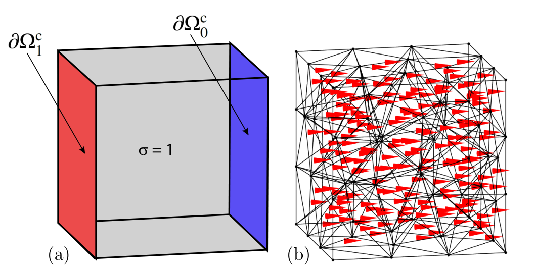
The patch tests are Poisson problems designed in such a way that their analytical solution is uniform. By interpreting the Poisson problems as direct current conduction problems, a simple way to produce a patch test is to consider a planar resistor, as described in Fig. 3(a). It has been verified that the $SP$, $VP=MH$, and $DSP$ formulations produce the analytical solution as represented in Fig. 3(b).

Figure 3: (a) The definition of a patch test as the solution of an electric conduction problem inside a planar resistor. (b) All mentioned formulations are able to retrieve the analytical solution up to machine precision or iterative solver tolerance.

5.4 Multi-material patch tests

The multi-material patch tests are direct current conduction problems designed in such a way that their solution is piecewise uniform. A simple way to produce multi-material patch test is to consider a resistor with two conductors with different material properties placed in series or in parallel as described in Fig. 4(a) and Fig. 4(d). A voltage of $u=1\,$V is enforced between the reference electrode $\partial\Omega^{\mathrm{c}}_{0}$ and the electrode $\partial\Omega^{\mathrm{c}}_{1}$.

Figure 4: (a) The series multi-material patch test. (b) Electrostatic field $\bm{E}$ obtained with the series. (c) Current density field $\bm{J}$ obtained with the series. (d) The parallel multi-material patch test. (e) Electric field $\bm{E}$ obtained with the parallel. (f) Current density field $\bm{J}$ obtained with the parallel.

In the first multi-material patch test, two different materials with different material properties are placed in series. From the result represented in Fig. 4(b-c), we conclude that the tangential component of the electric field $\bm{E}$ is conserved across the material interface, whereas the tangential component of the current density field $\bm{J}$ jumps. This result holds for all formulations.

In the second multi-material patch test, two different materials with different material properties are placed in parallel. From the result represented in Fig. 4(e-f), we conclude that the normal component of the current density $\bm{J}$ is conserved across the material interface, whereas the normal component of the electric field $\bm{E}$ jumps. This result holds for all formulations.

5.5 Square resistor benchmark

As a more complicated example, we compute the conductance $G$ of a square resistor [31], see Fig. 5(a). A voltage of $u=1\,$V is enforced between the reference electrode $\partial\Omega^{\mathrm{c}}_{0}$ and the electrode $\partial\Omega^{\mathrm{c}}_{1}$, which are placed in the two lateral surfaces of the solid square torus. The conductor placed inside the solid torus has an electrical conductivity $\sigma=1\,$S/m. This problem, like most industrial problems, exhibits a singular analytical solution. Yet, the analytical solution is available ($G=10.23409256\,$S). The conductance $G$ is extracted by computing the total dissipated power $P=G\,u^{2}=\int_{\Omega}\frac{|\bm{J}|^{2}}{\sigma}$ or alternatively by using the Ohm’s law $G=i/u$, where $i$ is the current that flows between the two electrodes.

Figure 5: (a) The geometry of the square resistor benchmark ($h=1\,$m, $d=4\,$m, and $l=2\,$m). The two electrodes are depicted in red and blue. (b) Thanks to the symmetry, the computational domain has been reduced to one in eight of the resistor.

We recall that the $VP$ and $MH$ formulations produce the same results given that they are algebraically equivalent [31]. The conductance of the square resistor has been evaluated by the $SP$, $VP=MH$, and $DSP$ formulations on refined grids. The results are collected in Fig. 6. First, it is interesting to note that the results relative to the scalar potential $SP$ and to the vector potential $VP$ or mixed-hybrid $MH$ formulations provide, respectively, the upper and lower bounds for the conductance [33], [29]. This property is called complementarity in the computational electromagnetics community [10], [31].

Figure 6: Results for the square resistor benchmark.

6 Conclusions

In this paper, we have proposed a new construction of sparse inverse edge and face mass matrices for arbitrary tetrahedral grids. The proposed framework unifies the construction of both mass matrices and their inverses and is based on novel geometric reconstruction formulas, from which, local mass matrices are defined as the sum of a consistent and a stabilization term. The consistent term is defined geometrically and explicitly, thus providing a sensible speedup and an easier implementation, whereas the stabilization term is constructed according to a well-established design strategy. The resulting expressions for both types of local mass matrices are highly symmetric, thus highlighting the duality relationship between the pair of grids. Global mass matrices are then constructed using a standard assembling process. In this way we obtain a sparse matrix representation also for the inverse mass matrix. This avoids explicitly computing the algebraic inverse of the mass matrix which is found to be typically dense. A key aspect of the proposed method is that being based on geometric elements of the barycentric dual grid, it can be applied to arbitrary tetrahedral grids. Two different strategies are proposed to deal with the case of problems involving discontinuous material parameters for the case where the interfaces are aligned with the tetrahedral grid, and an hybrid approach between the two is employed in practical applications. We tested the newly derived inverse mass matrices by solving a Poisson problem and we verified that patch test is passed, even when material discontinuities are present. A real case problem involving a square resistor benchmark is analyzed. Given that reconstruction formulas in each dual cell provide a first-order approximation of a vector field, we expect that first-order error estimates can be derived for the numerical scheme.

References

- [1] E. Tonti, On the formal structure of physical theories, Monograph of the Italian National Research Council, 1975.
- [2] K. S. Yee, Numerical Solution of Initial Boundary Value Problems Involving Maxwell’s Equations in Isotropic Media, IEEE Transactions on Antennas and Propagation 14 (3) (1966) 302–307.
- [3] E. Tonti, A direct discrete formulation of field laws: The cell method, CMES - Computer Modeling in Engineering and Sciences 2 (2) (2001) 237–258. doi:10.3970/cmes.2001.002.237.
- [4] M. Clemens, T. Weiland, Discrete electromagnetism with the finite integration technique, Progress in Electromagnetics Research 32 (2001) 65–87. doi:10.2528/PIER00080103.
- [5]
L. Codecasa, R. Specogna, F. Trevisan,
Base
functions and discrete constitutive relations for staggered polyhedral
grids, Comput. Meth. Appl. Mech. Eng. 198 (9) (2009) 1117 – 1123.
doi:https://doi.org/10.1016/j.cma.2008.11.021.
URL http://www.sciencedirect.com/science/article/pii/S0045782508004234 - [6]
A
new set of basis functions for the discrete geometric approach, J. Comput.
Phys. 229 (19) (2010) 7401 – 7410.
doi:https://doi.org/10.1016/j.jcp.2010.06.023.
URL http://www.sciencedirect.com/science/article/pii/S0021999110003384 - [7]
J. Bonelle, A. Ern,
Analysis of
compatible discrete operator schemes for elliptic problems on polyhedral
meshes, ESAIM: Mathematical Modelling and Numerical Analysis -
Modélisation Mathématique et Analyse Numérique 48 (2) (2014) 553–581.
doi:10.1051/m2an/2013104.
URL http://www.numdam.org/item/M2AN_2014__48_2_553_0 - [8] K. Lipnikov, G. Manzini, M. Shashkov, Mimetic finite difference method, J. Comput. Phys. 257 (PB) (2014) 1163–1227. doi:10.1016/j.jcp.2013.07.031.
- [9] A. Bossavit, Whitney forms: A class of finite elements for three-dimensional computations in electromagnetism, IEE Proceedings A: Physical Science. Measurement and Instrumentation. Management and Education. Reviews 135 pt A (8) (1988) 493–500. doi:10.1049/ip-a-1.1988.0077.
- [10] A. Bossavit, Computational Electromagnetism, Academic Press, 1998.
- [11] A. Bossavit, How weak is the “weak solution” in finite element methods?, IEEE Transactions on Magnetics 34 (5) (1998) 2429–2432.
- [12] E. Tonti, The mathematical structure of classical and relativistic physics. A general classification diagram, Birkhäuser, Basel, 2013.
- [13] T. Tarhasaari, L. Kettunen, A. Bossavit, Some realizations of a discrete hodge operator: a reinterpretation of finite element techniques [for em field analysis], IEEE Trans. Magn. 35 (3) (1999) 1494–1497.
- [14] L. Codecasa, M. Politi, Explicit, consistent, and conditionally stable extension of FD-TD to tetrahedral grids by FIT, IEEE Transactions on Magnetics 44 (6) (2008) 1258–1261. doi:10.1109/TMAG.2007.916310.
- [15] B. He, F. L. Teixeira, Differential forms, galerkin duality, and sparse inverse approximations in finite element solutions of maxwell equations, IEEE Transactions on Antennas and Propagation 55 (5) (2007) 1359–1368.
- [16] L. Codecasa, B. Kapidani, R. Specogna, F. Trevisan, Novel FDTD technique over tetrahedral grids for conductive media, IEEE Transactions on Antennas and Propagation 66 (10) (2018) 5387–5396. doi:10.1109/TAP.2018.2862244.
- [17]
N. Bell, L. N. Olson,
Algebraic
multigrid for k-form laplacians, Numerical Linear Algebra with Applications
15 (2-3) (2008) 165–185.
arXiv:https://onlinelibrary.wiley.com/doi/pdf/10.1002/nla.577, doi:10.1002/nla.577.
URL https://onlinelibrary.wiley.com/doi/abs/10.1002/nla.577 - [18]
A. Lemoine, J. Caltagirone, M. Azaïez, S. Vincent,
Discrete helmholtz-hodge
decomposition on polyhedral meshes using compatible discrete operators, J.
Sci. Comput. 65 (1) (2015) 34–53.
doi:10.1007/s10915-014-9952-8.
URL https://doi.org/10.1007/s10915-014-9952-8 - [19] A. N. Hirani, Discrete Exterior Calculus Thesis by, Tech. rep. (2003).
- [20]
R. Eymard, T. Gallouët, R. Herbin, andRaphà ele Herbin,
Handbook of Numerical
Analysis, 9780444503503. which appeared in Handbook of Numerical Analysis,
P.G. Ciarlet, J.L. Lions eds 7 (2000) 713–1020.
doi:10.1016/S1570-8659(00)07005.
URL https://hal.archives-ouvertes.fr/hal-02100732v2 - [21]
A. Gillette, C. Bajaj,
Dual
formulations of mixed finite element methods with applications,
Computer-Aided Design 43 (10) (2011) 1213 – 1221, solid and Physical
Modeling 2010.
doi:https://doi.org/10.1016/j.cad.2011.06.017.
URL http://www.sciencedirect.com/science/article/pii/S001044851100159X - [22] F. Bellina, R. Specogna, Diagonal material matrices for arbitrary simplicial meshes for solving poisson problems with one unknown per element, IEEE Transactions on Magnetics 56 (2) (2020) 1–4.
- [23] A. Bossavit, Mixed-hybrid methods in magnetostatics: complementarity in one stroke, IEEE Transactions on Magnetics 39 (3) (2003) 1099–1102.
- [24] M. S. Mohamed, A. N. Hirani, R. Samtaney, Numerical convergence of discrete exterior calculus on arbitrary surface meshes, International Journal for Computational Methods in Engineering Science and Mechanics 19 (3) (2018) 194–206.
- [25] J. Bonelle, D. A. Di Pietro, A. Ern, Low-order reconstruction operators on polyhedral meshes: Application to compatible discrete operator schemes, Computer Aided Geometric Design 35-36 (2015) 27–41. doi:10.1016/j.cagd.2015.03.015.
- [26] P. B. Bochev, J. M. Hyman, Principles of Mimetic Discretizations of Differential Operators, in: Compatible Spatial Discretizations, Springer New York, 2007, pp. 89–119. doi:10.1007/0-387-38034-5_5.
- [27] J. Munkres, Elements of algebraic topology, Perseus Books, Cambridge, MA, 1984.
- [28] M. Berger, M. Cole, S. Levy, Geometry I, Universitext, Springer Berlin Heidelberg, 2009.
- [29]
R. Specogna,
Complementary
geometric formulations for electrostatics, Int. J. Numer. Meth. Eng. 86 (8)
(2011) 1041–1068.
arXiv:https://onlinelibrary.wiley.com/doi/pdf/10.1002/nme.3089,
doi:10.1002/nme.3089.
URL https://onlinelibrary.wiley.com/doi/abs/10.1002/nme.3089 - [30]
F. Brezzi, K. Lipnikov, M. Shashkov, V. Simoncini,
new discretization methodology for diffusion problems on generalized
polyhedral meshes, Comput. Meth. Appl. Mech. Eng. 196 (37) (2007) 3682 –
3692.
doi:https://doi.org/10.1016/j.cma.2006.10.028.
URL http://www.sciencedirect.com/science/article/pii/S0045782507000965 - [31] R. Specogna, One stroke complementarity for poisson-like problems, IEEE Trans. Magn. 51 (3) (2015) 1–4.
- [32] M. VohralÍík, B. I. Wohlmuth, Mixed finite element methods: implementation with one unknown per element, local flux expressions, positivity, polygonal meshes, and relations to other methods, Math. Mod. Meth. Appl. S. 23 (05) (2013) 803–838.
- [33] J. Synge, The hypercircle in mathematical physics, Cambridge University Press, Cambridge, 1957.