Inference of proto-neutron star properties from gravitational-wave data in core-collapse supernovae

Abstract

The eventual detection of gravitational waves from core-collapse supernovae (CCSN) will help improve our current understanding of the explosion mechanism of massive stars. The stochastic nature of the late post-bounce gravitational wave signal due to the non-linear dynamics of the matter involved and the large number of degrees of freedom of the phenomenon make the source parameter inference problem very challenging. In this paper we take a step towards that goal and present a parameter estimation approach which is based on the gravitational waves associated with oscillations of proto-neutron stars (PNS). Numerical simulations of CCSN have shown that buoyancy-driven g-modes are responsible for a significant fraction of the gravitational wave signal and their time-frequency evolution is linked to the physical properties of the compact remnant through universal relations, as demonstrated in [1]. We use a set of 1D CCSN simulations to build a model that relates the evolution of the PNS properties with the frequency of the dominant g-mode, which is extracted from the gravitational-wave data using a new algorithm we have developed for our study. The model is used to infer the time evolution of a combination of the mass and the radius of the PNS. The performance of the method is estimated employing simulations of 2D CCSN waveforms covering a progenitor mass range between 11 and 40 solar masses and different equations of state. Considering signals embedded in Gaussian gravitational wave detector noise, we show that it is possible to infer PNS properties for a galactic source using Advanced LIGO and Advanced Virgo data at design sensitivities. Third generation detectors such as Einstein Telescope and Cosmic Explorer will allow to test distances of ${\cal O}(100\,{\rm kpc})$.

I Introduction

The life of sufficiently massive stars, i.e. those born with masses between $\sim 8$ M_⊙ and $\sim 120$ M_⊙, ends with the collapse of the iron core under its own gravity, leading to the formation of a neutron star (NS) or a black hole (BH), and followed (typically but not necessarily in the BH case) by a supernova explosion. Nearby core-collapse supernova (CCSN) explosions are expected to be sources of gravitational waves (GWs) and they could be the next great discovery of current ground-based observatories. However, these are relative rare events. A neutrino-driven explosion [2] is the most likely outcome in the case of slowly rotating cores, which are present in the bulk of CCSN progenitors. The emitted GWs could be detected with the advanced ground-based GW detector network, Advanced LIGO (aLIGO) [3], Advanced Virgo (AdV) [4] and KAGRA [5], within $\sim$ 5 kpc [6, 7]. Such a galactic event has a rate of about $2-3$ per century [8, 9]. For the case of rapidly rotating progenitor cores the result is likely a magneto-rotational explosion, yielding a more powerful GW signal that could be detected within 50 kpc and, for some extreme models, up to 5–30 Mpc [6, 7]. However, only about $1\%$ of the electromagnetically observed events show signatures of fast rotation (broad-lined type Ic SNe [10] or events associated with long GRBs [11]) making this possibility a subdominant channel of detection with a galactic event rate of $\sim$ $10^{-4}$ $\rm{yr}^{-1}$. Despite the low rates, CCSN are of great scientific interest because they produce complex GW signals which could provide significant clues about the physical processes at work after the gravitational collapse of stellar cores.

In the last decade significant progress has been made in the development of numerical codes, in particular in the treatment of multidimensional effects [12]. In the case of neutrino-driven explosions, the GW emission is primarly induced by instabilities developed at the newly formed proto-neutron star (PNS) and by the non-spherical accreting flow of hot matter over its surface [13]. These dynamics excite the different modes of oscillation of the PNS which ultimately leads to the emission of GWs. The frequency and time evolution of these modes carry information about the properties of the GW emitter and could allow to perform PNS asteroseismology.

All multidimensional numerical simulations show the systematic appearance in time-frequency diagrams (or spectrograms) of a distinct and relatively narrow feature during the post-bounce evolution of the system, with frequency rising from about 100 Hz up to a few kHz (at most) and a typical duration of 0.5 – 1 s. This feature has been interpreted as a continuously excited gravity mode (g-mode, see [14, 15] for a definition in this context) of the PNS [16, 17, 18, 19, 20, 21]. In these models the monotonic raise of the frequency of the mode is related to the contraction of the PNS. The typical frequencies of these modes make them interesting targets for ground-based GW interferometers.

The properties of g-modes in hot PNSs have been studied since the 1990s by means of linear perturbation analysis of background PNS models. The oscillation modes connected with the surface of hot PNSs were first considered by McDermott et al. [22]. Additionally, the stratified structure of the PNS allows for the presence of different types of g-modes related to the fluid core [23]. Many subsequent works used simplified neutron star models assuming an equilibrium configuration as a background, to study the effect of rotation [24], general relativity [25], non-linearities [26], phase transitions [27] and realistic equation of state [28]. Only recently, there have been efforts to incorporate more suitable backgrounds based on numerical simulations in the computation of the mode structure and evolution [29, 30, 31, 32, 1, 33, 34, 35, 36].

Using results from 2D CCSN numerical simulations as a background [30, 32] found that the eigenmode spectrum of the region within the shock (including the PNS and the post-shock region) shows a good match to the mode frequencies and to the features observed in the GW spectrum of the same simulations (specially when space-time perturbations are included [32]).

This reveals that it is posible to perform CCSN asteroseismology under realistic conditions and serves as a starting point to carry out inference of astrophysical parameters of PNSs. Further work was presented in [1] who found that it is possible to derive simple relations between the instantaneous frequency of the g-mode and the mass and radius of the PNS at each time of the numerical evolutions. These relations are universal as they do not depend on the equation of state (EOS) or on the mass of the progenitor and they only depend weakly on the numerical code used (see discussion in Section II). Similar universal relations have been discussed by [35, 36] who also found that they do not depend on the dimensionality (1D, 2D or 3D) of the numerical simulation used as a background.

Previous data analysis efforts have focused on the reconstruction of the GW strain amplitude without assuming a particular signal model [37, 38, 39]. As the amount of numerical simulations increased other methods using waveform catalogs have been proposed to identify the supernova explosion mechanism. Among them, principal component analysis helps at reducing the complexity of CCSN waveforms to fewer parameters [40, 41, 42, 43, 44, 45]. The classification challenge is also well addressed with deep learning methods [46, 47].

In this work we introduce a method to infer PNS properties, namely a combination of the mass and radius, using GW information. For this purpose we have developed an algorithm to extract the time-frequency evolution of the main feature in the spectrograms of the GW emission of 2D simulations of CCSN. This feature corresponds to the ${}^{2}\rm{g}_{2}$ mode, according to the nomenclature used in [1] (different authors may have slightly different naming convention). Next, we use the universal relations obtained by [1], based on a set of 1D simulations, to infer the time evolution of the ratio $M_{\rm PNS}/R_{\rm PNS}^{2}$ (the PNS surface gravity), where $M_{\rm PNS}$ and $R_{\rm PNS}$ are the mass and the radius of the PNS. Finally, using 2D CCSN waveform corresponding to different progenitor masses we estimate the performance of the algorithm for current and future generation of ground-based GW detectors.

This paper is organized as follows. Section II provides details of the CCSN simulations used in our work. The algorithm that we employ to extract the time evolution of the PNS surface gravity is discussed in Section III. Section IV shows the performance of our inference method and presents our main results. Finally, our findings are summarized in Section V. Appendix A discusses specific details related to the reconstruction of the g-mode.

II Core collapse supernova simulations

Unlike other methods used in GW astronomy the algorithm proposed in this work does not require accurate waveforms in order to infer the properties of the PNS. Instead, it relies on the evolution of the oscillation frequency of some particular modes visible in the GW spectrum. The frequency of these modes depends in a universal way on the surface gravity of the PNS, $r\equiv M_{\rm PNS}/R_{\rm PNS}^{2}$ [1]. Therefore, if at a given time GW emission is observed at a certain frequency $f$ then the value of the surface gravity can be determined unequivocally, within a certain error, regardless of the details of the numerical simulation.

In this work we use two sets of simulations: i) the model set, composed by 1D simulations, which is used to build the universal relation (model), $r(f)$, linking the ratio $r$ with the observed frequency $f$, and ii) the test set, composed by 2D simulations, for which we know both the GW signal and the evolution of the ratio, $r(t)$, and that is used to test performance of the algorithm.

Both the model set and test set simulations have been generated using the AENUS-ALCAR code [48] which combines special relativistic (magneto-)hydrodynamics, a modified Newtonian gravitational potential approximating the effects of general relativity [49], and a spectral two-moment neutrino transport solver [48]. All siimulations include the relevant reactions between matter and neutrinos of all flavours, i.e., emission and absorption by nucleons and nuclei, electron-positron pair annihilation, nucleonic bremsstrahlung, and scattering off nucleons, nuclei, and electrons.

For the model set, we use the $18$ spherically symmetric (1D) simulations of [32] including progenitors with zero-age main sequence (ZAMS) masses in the range $M_{\mathrm{ZAMS}}=$ 11.2 – 75 $M_{\odot}$. The set contains simulations using six different EOS. Details can be found in [32]. The reason to use 1D simulations for the model set is that their computational cost is significantly smaller than that of multidimensional simulations which allows us to accumulate the statistics necessary to build a good model for $r(f)$. For each time of each simulation we compute the ratio $r$ and the frequency of the ${}^{2}g_{2}$ mode by means of the linear analysis described in [30, 32, 1].

Model	$M_{\mathrm{ZAMS}}$	progenitor	EOS	$t_{\mathrm{f}}$	$t_{\rm explosion}$	$M_{\mathrm{PNS,f}}$
name	$[M_{\odot}]$	model		$[\mathrm{s}]$		$[M_{\odot}]$
s11	11.2	[50]	LS220	1.86	$\times$	1.47
s15	15.0	[50]	LS220	1.66	$\times$	2.00
s15S	15.0	[50]	SFHo	1.75	$\times$	2.02
s15G	15.0	[50]	GShen	0.97	$\times$	1.86
s20	20.0	[50]	LS220	1.53	$\times$	1.75
s20S	20.0	[51]	SFHo	0.87	$\times$	2.05
s25	25.0	[50]	LS220	1.60	$0.91$	2.33
s40	40.0	[50]	LS220	1.70	$1.52$	2.23

Table 1: List of axisymmetric simulations used for the test set. The last three columns show, the post-bounce time at the end of the simulation, the one at the onset of the explosion (non exploding models marked with $\times$), and the PNS mass at the end of the simulation.

For the test set, we use $8$ axisymmetric (2D) simulations performed with the AENUS-ALCAR code (see Table 1 for a list of models). All of these simulations but model s20S use a selection of progenitors with masses in the range $M_{\mathrm{ZAMS}}=$ 11.2 – 40 $M_{\odot}$ evolved through the hydrostatic phases by [50]. We performed one simulation of each stellar model using the EOS of [52] with an incompressibility of $K=$ 220 MeV (LS220) and added comparison simulations with the SFHo EOS [53] and the GShen EOS [54] for the progenitor with $M_{\mathrm{ZAMS}}=$ 15 $M_{\odot}$. To this set of simulations we add the waveform of a 2D model used in [32], denoted s20S. It corresponds to a star with the same initial mass, $M_{\mathrm{ZAMS}}=$ 20 $M_{\odot}$, as for one of the other seven axisymmetric simulations, but was taken from a newer set of stellar-evolution models [51]. It was evolved with the SFHo EOS.

For all the simulations, we mapped the pre-collapse state of the stars to a spherical coordinate system with $n_{r}=400$ zones in the radial direction distributed logarithmically with a minimum grid width of $(\Delta r)_{\mathrm{min}}=$ 400 m and an outer radius of $r_{\mathrm{max}}=$ $8.3\times 10^{9}$ cm and $n_{\theta}=128$ equidistant cells in the angular (polar) direction. For the neutrino energies, we used a logarithmic grid with $n_{e}=10$ bins up to 240 MeV. Unlike the model set, the simulations in the test set are not 1D because we need to extract the GW signal, which is a multi-dimensional effect. For each simulation the GW signal, $h_{+}(t)$, is extracted by means of the quadrupole formula and we compute the time evolution of the surface gravity, $r(t)$.

All spherical and most axisymmetric models we evolved fail to achieve shock revival during the time of our simulations. Only the two stars with the highest masses, s25 and s40, develop relatively late explosions in axisymmetry. Consequently, mass accretion onto the PNSs proceeds at high rates for a long time in all cases and causes them to oscillate with their characteristic frequencies. The final masses of the PNSs are in the range of $M_{\mathrm{PNS}}=$ 1.47 – 2.33 $M_{\odot}$, i.e., likely insufficient for producing a black hole.

III Description of the method

Figure 1: Ratio $M_{\rm PNS}/R_{\rm PNS}^{2}$ from our 18 1D simulations of the model set. The solid line is the maximum likelihood estimate of heteroscedastic cubic model with 95% confidence bands (dashed lines) considering the 18 simulation data points.

We next outline our strategy for estimating the time evolution of $r(t)$ from the observation of the $\mbox{}^{2}g_{2}$ oscillation mode in the GW detector data. To build the model of the ratio $r$ as a function of the frequency $f$ we use the 1D simulations of the model set. Figure 1 shows the data for the $18$ numerical simulations. Using these data we parametrize the discretized ratio $r_{i}$ with a cubic polynomial regression with heteroscedastic errors

$$r_{i}=\beta_{1}f_{i}+\beta_{2}f_{i}^{2}+\beta_{3}f_{i}^{3}+\epsilon_{i}\,,$$ (1)

where $\epsilon_{i}$ are assumed to be independent zero-mean Gaussian errors with variances $\sigma_{i}^{2}$ that increase with frequency $f_{i}$. The model for frequency-dependent variances is

$$\log\sigma_{i}=\alpha_{0}+\alpha_{1}f_{i}+\alpha_{2}f_{i}^{2}+\delta_{i}\,,$$ (2)

with independent and identically zero-mean Gaussian errors $\delta_{i}$. The R-package lmvar [55] that implements a maximum likelihood approach was used to fit the model.

The best fitting model amongst polynomials of degree 1, 2, and 3 was chosen according to the Akaike information criterion with coefficients given in Table 2, which is actually the model defined in (1). The data and fit of the model including 95% confidence bands are displayed in Figure 1.

Coefficient	Estimate	Standard error
$\beta_{1}$	$2.00\times 10^{-06}$	$4.23\times 10^{-08}$
$\beta_{2}$	$-1.64\times 10^{-9}$	$9.99\times 10^{-11}$
$\beta_{3}$	$2.03\times 10^{-12}$	$5.41\times 10^{-14}$
$\alpha_{0}$	$-9.54\times 10^{+00}$	$6.80\times 10^{-02}$
$\alpha_{1}$	$7.24\times 10^{-04}$	$1.56\times 10^{-04}$
$\alpha_{2}$	$6.23\times 10^{-07}$	$8.15\times 10^{-08}$

Table 2: Estimate and standard error of the coefficients of the best fit model describing the ratio $r=M_{\rm PNS}/R_{\rm PNS}^{2}$ as function of the frequency of the $\mbox{}^{2}g_{2}$ mode.

We use this model to infer the properties of the simulations in the test set discussed in Section II. To describe the method we focus on the GW signal of model s20S, originally sampled at 16384 Hz but downsampled at 4096 Hz. A spectrogram of this signal is shown in Figure 2 based on autoregressive estimates [56] of the local spectra for successive time intervals of length 200 with a 90% overlap. The dominant emission mode corresponds to the PNS oscillation $\mbox{}^{2}g_{2}$-mode. We have developed a time-frequency method to track the ridge $m(t)$ in the spectrogram, taking into account that it is monotonically increasing with time. This is a property of the $\mbox{}^{2}g_{2}$-mode whose frequency increases as the PNS becomes more massive and compact. Starting from either the left- or right-most column of the time-frequency matrix we identify and trace the sequence of amplitude peaks within a certain frequency band given the monotonicity constraint. Specific details about the reconstruction of the $\mbox{}^{2}g_{2}$-mode ridge are provided in Appendix A.

Figure 2: Spectrogram of the GW signal s20S sampled at 4096 Hz. The spectrogram is obtained using a data streach of 200 samples overlapping at 90% with each other. The open circles track the ridge $m(t)$ of the $\mbox{}^{2}g_{2}$-mode.

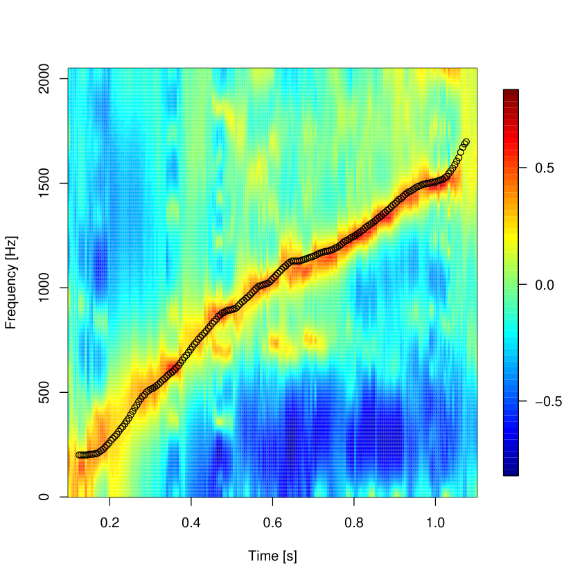
We collect the instantaneous frequency $f(t_{i})$ corresponding to the ridge $m(t_{i})$ for the midpoint $t_{i}$ of each local time interval of the spectrogram and interpolate $f(t)$ for values in between $t_{i}$. We then use our model given by Eq. (1) to obtain estimates of the time evolution of the ratio together with 95% confidence intervals. An example is given in Figure 3 where the red triangles are the point estimates and the grey bands represent 95% confidence bands. The size of the red triangles is proportional to the magnitude of the $\mbox{}^{2}g_{2}$-mode frequency estimates. Note that as the frequency of the $\mbox{}^{2}g_{2}$-mode becomes higher our estimates show more uncertainty (bigger intervals) because our model allows for heterogeneous variance. Ratio values computed using the mass and radius values obtained from the simulation code (i.e. the true values) are shown in black. In this example of a well detectable GW signal the coverage of our 95% confidence band is 100% of the true values. In the next section we investigate the performance of the reconstruction of $r(t)$ when the GW signal is embedded in noise. We also note that despite we have only explicitely shown results for the GW signal of the s20S model the same conclusions hold for any of the other waveforms of our test set.

Figure 3: Comparison of the time evolution of the ratio $M_{\rm PNS}/R_{\rm PNS}^{2}$ estimated from the $\mbox{}^{2}g_{2}$-mode of the s20S signal (shown by open triangles and by the 95% confidence belt in grey) against the value derived from the PNS mass and radius given by the simulation code (shown by filled black circles). The size of the triangles are represented proportionally to the magnitude of the $\mbox{}^{2}g_{2}$-mode frequency estimates.

IV Detectability prospects

Figure 4: Boxplots of the $coverage$ (upper panel) and $\Delta$ (lower panel) for s20S signal embedded in aLIGO noise at different distances from the Earth. 100 noise realizations are considered for each distance. The orange lines indicate the median values while the empty rectangles indicate the first and third quartiles. The “+” markers are outliers outside the first and third quartiles.

To estimate how accurately we can infer the time evolution of $r(t)$ in the GW data of a single detector we inject the GW signal for model s20S into 100 Gaussian noise realisations whose power spectral density (PSD) follows the aLIGO spectrum [57].

We cover a large range of distances for which a CCSN detection in second-generation GW detectors is feasible. We assume that the source is optimally oriented with respect to our single detector. Moreover, we also assume that a CCSN GW signal has been identified in the data and that the beginning of the signal is known within $\mathcal{O}$(10 ms). The data (signal embedded in noise) are whitened using the function prewhiten of the R-package TSA. An auto-regressive model with a maximum of maximal 100 coefficients is used.

For each of the noise realizations we reconstruct the track ridge $m(t_{i})$ starting from the left side of the spectrogram and constraining the beginning of the track to be smaller than 200 Hz. This value is chosen using the information on the initial mode frequency from the simulations. We derive the ratio time series $r_{i}$ of length $N$ which is then compared to the “true” ratio $r_{i}^{0}$ derived from the PNS mass and radius computed from the s20S simulation. The top panel of Fig. 4 shows the distribution of the fraction of the ratio values $r_{i}^{0}$ that fall within the 95% confidence interval of $r_{i}$ as a function of the distance to the source. This quantity, hence, gives information about the coverage of the reconstructed ratio. The coverage takes maximum values when the source is located within a few kpc and then decreases with the distance.

To better quantify how well we reconstruct the ratio we also consider the mean of the relative error of $r_{i}$ along the track of the spectrogram, $\Delta$,

$$\Delta=\frac{1}{N}\sum_{1}^{N}\frac{|r_{i}-r_{i}^{0}|}{r_{i}^{0}}\,.$$ (3)

The values of $\Delta$ for each of the 100 noise realizations are shown as a function of the distance in the bottom panel of Fig. 4. For a source located up to $\sim$9 kpc the relative error remains smaller than 20%. At closer distances $\Delta$ is smaller but it does not vanish. This reflects the approximate nature of the model used for $r$. It is nevertheless remarkable that, on average, one can reconstruct the ratio time series with a good precision up to distances of $\sim$ 9 kpc (for this particular waveform) with a coverage value larger than 80%. We note that there are a few noise realizations for distances below 9 kpc for which $\Delta$ takes large values, indicating that the method fails to accurately reconstruct the ratio in those cases. The main cause of failure is the split of the ridge in few blobs when the signal becomes weaker and weaker.

Figure 5: Data points (“+”) show the median of the coverage for the eight CCSN waveforms of the test set embedded in aLIGO noise as a function of the distance to the source. The solid lines are smoothing splines. The “no signal” line shows the median of coverage in absence of any signal. In this example, the median is null and overlaps with the horizontal axis. The blue band boundaries are given by the $\mathrm{5^{th}}$ and $\mathrm{95^{th}}$ percentiles of coverage in absence of any signal.

Figure 6: Data points (“+”) show the median of the relative error $\Delta$ for the eight CCSN waveforms of the test set embedded in aLIGO noise as a function of the distance to the source. The solid lines are smoothing splines. The “no signal” line shows the median of $\Delta$ in absence of any signal. The blue band boundaries are given by the $\mathrm{5^{th}}$ and $\mathrm{95^{th}}$ percentiles of $\Delta$ in absence of any signal.

We have tested that the method does not depend on the specific features of the waveform of model s20S by repeating the procedure for the remaining seven waveforms of the test set described in Section II covering a large range of progenitor masses. Figure 5 shows that apart from model s11 and to a lesser extent model s20S, the ratio is well reconstructed for all waveforms up to a distance of $\sim$ 15kpc. In an effort to better determine the maximal distance of the source at which we can reconstruct the ratio we have run 100 simulations without injecting a signal and have measured the corresponding coverage for the reconstructed ratios. The median of the coverage as well as the band defined by the $\mathrm{5^{th}}$ and $\mathrm{95^{th}}$ percentiles are shown in Figure 5. The noise only median value is identically zero in this case. However, note that it could be different from zero because the g-mode reconstruction algorithm is looking for a continuously increasing frequency track in the spectrogram, starting between 0 and 200 Hz, where we expect the GW signal to be. This is enhancing the probability of overlap. This effect explains why certain values of overlap can reach values as high as 80% even when no signal is added to the noise.

Figure 6 shows the relative error $\Delta$ as a function of the distance for the signals of the test set as well as the result when only noise is considered. This quantity follows the same trend than that followed by the coverage, since all signals but models s11 and s20S are reconstructed with relative errors below 20% up to distances of $\sim$ 15kpc. Correspondingly, the no-signal case yields the largest error, as expected.

We perform the same analysis using the design sensitivity curve of AdV and expected sensitivity curves for third-generation GW detectors. The results for the former are reported in Table 3 and are discussed below. We focus now on third-generation detectors, presenting our findings in Table 3 and in Fig. 7. In Europe the Einstein Telescope project proposes to host in a 10-km equilateral triangle configuration three low-power, low-frequency, cryogenic interferometers as well as three high-power, high-frequency interferometers. Three sensitivity curves, ET_B, ET_C and ET_D corresponding to different options and stages of the project [58] are considered in our study. The US based project Cosmic Explorer [59] is expecting to reach its design sensitivity circa 2040 through two phases labeled CE1 and CE2.

Figure 7: Data points (“+”) show the median of the relative error $\Delta$ as a function of the distance to the source for the CCSN waveform model s20S embedded in third-generation detector noise. The solid lines are smoothing splines. The blue band boundaries are given by the $\mathrm{5^{th}}$ and $\mathrm{95^{th}}$ percentiles of coverage in absence of any signal for ET_D noise realisations.

Figure 7 displays $\Delta$ as a function of the source distance for the five third-generation detector configurations we analyze. As before, we use the s20S waveform model as a reference case. This figure shows that, overall, the ratio is well reconstructed up to distances in the range 100–200 kpc which represents an order of magnitude improvement with respect to aLIGO and AdV. We also note that the results for the various Einstein Telescope configurations lay in between those of the two Cosmic Explorer designs. Moreover, the detectability prospects for the former depend weakly on the detector configuration while the arrangement of CE2 yields better results than CE1. These results are confirmed for all other waveforms of our sample except for model s25 for which the maximal distance reach in CE2 is significantly lower than CE1, as shown in Fig. 8. This is partly due to the small variation of the reconstruction quality to the distance of the source making the estimation of $d_{r}$ rather uncertain for this particular waveform.

Figure 8: Maximal distance at which the ratio $r=M_{\rm PNS}/R_{\rm PNS}^{2}$ is reconstructed with good accuracy for all GW detectors analyzed in this study. The values are shown for all eight CCSN waveforms of our sample assuming that the source is optimally oriented with respect to the detector. Some waveform maximal distance markers are not visible because the do overlap (for instance s15G is overlapping with s25 for CE2).

		s11	s15	s15S	s15G	s20	s20S	s25	s40
aLIGO	$d_{r}$	7	28	24	22	16	11	38	46
	$d_{\rm det}$	11	36	26	27	21	16	74	61
AdV	$d_{r}$	7	26	20	19	15	10	43	42
	$d_{\rm det}$	10	32	22	23	18	13	64	52
CE1	$d_{r}$	79	304	258	229	187	115	524	490
	$d_{\rm det}$	115	377	270	282	217	168	774	633
CE2	$d_{r}$	135	499	451	405	305	183	391	898
	$d_{\rm det}$	197	649	468	489	375	294	1347	1100
ET_B	$d_{r}$	71	293	248	245	158	123	113	392
	$d_{\rm det}$	106	364	274	391	216	200	805	665
ET_C	$d_{r}$	75	302	239	237	172	131	239	446
	$d_{\rm det}$	97	332	246	260	194	164	727	603
ET_D	$d_{r}$	83	329	257	261	186	139	369	523
	$d_{\rm det}$	107	368	271	285	213	174	796	661

Table 3: Maximal distance $d_{r}$ at which the ratio $r=M_{\rm PNS}/R_{\rm PNS}^{2}$ is reconstructed with good accuracy for all GW detectors analyzed in this study, assuming optimal orientation between the source and the detector. Correspondingly, $d_{\rm det}$ is the distance at which different interferometers could detect a source optimally oriented with a matched filter signal-to-noise ratio of 13. All distances are expressed in kpc.

All results for both second-generation and third-generation detectors are summarized in Table 3 and Figure 8. Table 3 reports the source distances $d_{r}$ in kpc at which the median of the coverage is lower than 95% of the noise only values for aLIGO, AdV, and different configurations of third-generation detectors. This same information is displayed in Fig. 8. We have checked that using either the median of the coverage or the median of $\Delta$ yields similar results for the distance. On the other hand, the quality of the ratio reconstruction and, thus, of the distance range, depends on the signal-to-noise ratio, expressed in Table 3 by $d_{\rm det}$. The numbers reported on the table for $d_{r}$ are an estimate of the order of magnitude of the maximal distance of the source at which a reconstruction of the ratio could be possible with current and planned GW detectors. We also provide upper limits for $d_{\rm det}$ by taking into account the detector antenna response in our simulations and assuming that the source is optimally oriented with a matched filter signal-to-noise ratio of 13. Table 3 shows that the results for the AdV detector at design sensitivity are very similar to those of aLIGO, despite the differences in detector sensitivity. It is remarkable that for third-generation detectors the PNS surface gravity could be reconstructed for sources located up to a few hundreds of kpc. It is nevertheless important to note the rather wide range in distances we obtain for the different waveforms of our test set that probe a large range of progenitor masses. We do not find any correlation between either the mass of the progenitor nor the EOS with $d_{r}$.

V Conclusions

The detection of GW from CCSN may help improve our current understanding of the explosion mechanism of massive stars. In this paper we have proposed an exploratory method to infer PNS properties using an approach based on GW associated with convective oscillations of PNS. As shown by [1] buoyancy-driven g-modes are excited in numerical simulations of CCSN and their time-frequency evolution is linked to the physical properties of the compact remnant through universal relations. Such modes are responsible for a significant fraction of the highly stochastic GW emitted after core bounce. The findings reported in this paper suggest that PNS asteroseismology might be within reach of current and third-generation GW detectors.

In our study we have used a set of 1D CCSN simulations to build a model that relates the evolution of PNS properties with the frequency of the dominant g-mode, namely the $\mbox{}^{2}g_{2}$ mode. This relationship is extracted from the GW data using an algorithm developed for this investigation. This algorithm is a first attempt to infer the time evolution of a particular combination of the PNS mass and radius based on the universal relations found in [1]. More precisely, we have considered the ratio $r=M_{\rm PNS}/R_{\rm PNS}^{2}$ (the PNS surface gravity) derived from the observation of the $\mbox{}^{2}g_{2}$ oscillation mode in the numerically generated GW data. The performance of our method has been estimated employing simulations of 2D CCSN waveforms covering a progenitor mass range between 11 and 40 solar masses and different equations of state.

We have investigated the performance of the algorithm in the case of an optimally oriented source detected by a singe GW detector. Our numerical signals have been injected into 100 Gaussian noise realisations whose PSD follow the spectra of the different GW detectors analyzed. We have found that for Advanced LIGO and Advanced Virgo, the ratio $r$ can be reconstructed with a good accuracy in the case of a galactic CCSN (i.e. for distances of ${\cal O}(10\,{\rm kpc})$). This holds for a wide range of progenitor masses, the quality of the inference mainly depending on the signal-to-noise ratio of the event. For third-generation GW detectors such as the Einstein Telescope and the Cosmic Explorer, however, we obtain an order of magnitude improvement, as the $\mbox{}^{2}g_{2}$ ratio can be reconstructed for sources at distances of ${\cal O}(100\,\mathrm{kpc})$. In particular, Cosmic Explorer in its stage 2 configuration yields the best performance for all waveforms we have considered thanks to its excellent sensitivity in the 100-1000 Hz range. Among the three configurations of the Einstein Telescope, ET-D provides the best performance, especially for our set waveforms with the highest progenitor masses (25 $M_{\odot}$ and 40 $M_{\odot}$). Comparing the estimated distances for ET-B and the other third-generations detectors, having a good sensitivity below 200 Hz seems the most important factor to detect high mass progenitor signals.

In the present study we have assumed that the sources are optimally oriented. The reported distances at which we can infer the time evolution of $M_{\rm PNS}/R_{\rm PNS}^{2}$ must thus be regarded as upper limits. Those figures may decrease by a factor 2–3 on average for a source located anywhere in the sky. Furthermore, we have not considered the detectability prospects of CCSN waveforms in the realistic case in which the interferometers operated as a detector network. We defer an improved implementation of our approach for a forthcoming publication. Finally, we note that the method discussed in this work can be adapted to other PNS oscillation modes, by simply changing a few parameters such as the initial frequency range of the mode and its monotonic raise or descent. Being able to reconstruct several modes in the same GW signal would potentially allow to individually infer the mass and the radius of the PNS in core-collapse supernova explosions.

Acknowledgments.– Work supported by the Spanish Agencia Estatal de Investigación (PGC2018-095984-B-I00), by the Generalitat Valenciana (PROMETEO/2019/071) and by the European Union’s Horizon 2020 research and innovation (RISE) programme (H2020-MSCA-RISE-2017 GrantNo. FunFiCO-777740). N.C. acknowledges support from National Science Foundation grant PHY-1806990. R.M. gratefully acknowledges support by the James Cook Fellowship from Government funding, administered by the Royal Society Te Apārangi. R.M. and P.M.-R. also acknowledge funding from DFG Grant KI 1443/3-2 and thank the Centre for eResearch at the University of Auckland for their technical support. P.C.-D. acknowledges the support of the Spanish Ramon y Cajal programme (RYC-2015-19074) supporting his research.

Appendix A g-mode reconstruction

Given the spectrogram and a prescribed time interval for the ${}^{2}g_{2}$-mode reconstruction, our proposed method works as follows. The starting point must be specified. It can be either at the beginning or at the end of the signal. Then, in one of these two extremes, the maximum energy value is identified, registering its frequency. This is done independently for a number of consecutive time intervals. Then, we calculate the median of these frequency values, providing a robust starting value for the ${}^{2}g_{2}$-mode reconstruction.

The starting frequency value is the first ${}^{2}g_{2}$-mode estimate for the first or the last time interval, depending on the starting location we choose. If the reconstruction is set to start at the beginning of the signal, the reconstruction will be done progressively over the time intervals, where each maximum frequency value will be calculated within a frequency range specified by the previous ${}^{2}g_{2}$-mode estimate. Given the non-decreasing behaviour of the true ${}^{2}g_{2}$-mode values, the mode estimates will be forced to be greater or equal than the one estimated for its previous time interval, and lower than a specified upper limit. As a result, the ${}^{2}g_{2}$-mode estimates will be a non-decreasing sequence of frequency values. Then, the moving average is applied for smoothing the estimates.

If the reconstruction is set to start at the end of the signal, the ${}^{2}g_{2}$-mode will be estimated backward in time. Each maximum frequency is calculated within a range determined by its successor (in time) mode estimate. These estimates are forced to be lower or equal than its successor (in time) estimate, but greater than a specified lower limit. Thus, a non-decreasing sequence of ${}^{2}g_{2}$-mode estimates is guaranteed. Then, the moving average is applied for smoothing the estimates. This ${}^{2}g_{2}$-mode reconstruction method works if and only if the signal is strong enough to provide information about the mode, which is reflected in the spectrogram.

Given the sequence of ${}^{2}g_{2}$-mode estimates, the confidence band will be calculated by using the model defined in Eq. (1). The ${}^{2}g_{2}$-mode estimates are frequency values which we use as predictors in the model in order to generate confidence intervals for the ratios. Since the mode estimates are indexed by time, the confidence intervals for the ratios are too. Thus, we generate the confidence band by interpolating the lower and upper limits of the collection of consecutive confidence intervals, which will be valid for the time range of the ${}^{2}g_{2}$-mode estimates. This confidence band is used to estimate the coverage probabilities in our simulation studies presented in the main text.

References

- [1] A. Torres-Forné, P. Cerdá-Durán, M. Obergaulinger, B. Müller, and J. A. Font, “Universal Relations for Gravitational-Wave Asteroseismology of Protoneutron Stars,” Phys. Rev. Lett. 123, 051102 (2019), arXiv:1902.10048 [gr-qc] .
- [2] H. A. Bethe, “Supernova mechanisms,” Rev. Mod. Phys. 62, 801–866 (1990).
- [3] J. Aasi et al. (LIGO Scientific Collaboration), “Advanced LIGO,” Class. Quant. Grav. 32, 074001 (2015), arXiv:1411.4547 [gr-qc] .
- [4] F. Acernese et al. (Virgo Collaboration), “Advanced Virgo: a second-generation interferometric gravitational wave detector,” Class. Quant. Grav. 32, 024001 (2015), arXiv:1408.3978 [gr-qc] .
- [5] Y. Aso, Y. Michimura, K. Somiya, M. Ando, O. Miyakawa, T. Sekiguchi, D. Tatsumi, and H. Yamamoto (KAGRA), “Interferometer design of the KAGRA gravitational wave detector,” Phys. Rev. D 88, 043007 (2013), arXiv:1306.6747 [gr-qc] .
- [6] S. E. Gossan, P. Sutton, A. Stuver, M. Zanolin, K. Gill, and C. Ott, “Observing gravitational waves from core-collapse supernovae in the advanced detector era,” Physical Review D 93 (2016), 10.1103/physrevd.93.042002.
- [7] B. P. Abbott et al. (LIGO Scientific and Virgo Collaboration), “Optically targeted search for gravitational waves emitted by core-collapse supernovae during the first and second observing runs of advanced LIGO and advanced Virgo,” Phys. Rev. D 101, 084002 (2020), arXiv:1908.03584 [astro-ph.HE] .
- [8] S. M. Adams, C. S. Kochanek, J. F. Beacom, M. R. Vagins, and K. Z. Stanek, “Observing the Next Galactic Supernova,” Astrophys. J. 778, 164 (2013), arXiv:1306.0559 [astro-ph.HE] .
- [9] K. Rozwadowska, F. Vissani, and E. Cappellaro, “On the rate of core collapse supernovae in the milky way,” New Astronomy 83, 101498 (2021), arXiv:2009.03438 [astro-ph.HE] .
- [10] W. Li, J. Leaman, R. Chornock, A. V. Filippenko, D. Poznanski, M. Ganeshalingam, X. Wang, M. Modjaz, S. Jha, R. J. Foley, and N. Smith, “Nearby supernova rates from the Lick Observatory Supernova Search - II. The observed luminosity functions and fractions of supernovae in a complete sample,” Mon. Not. Roy. Astron. Soc. 412, 1441–1472 (2011), arXiv:1006.4612 [astro-ph.SR] .
- [11] R. Chapman, N. R. Tanvir, R. S. Priddey, and A. J. Levan, “How common are long gamma-ray bursts in the local Universe?” Mon. Not. Roy. Astron. Soc. 382, L21–L25 (2007), arXiv:0708.2106 [astro-ph] .
- [12] B. Müller, “Hydrodynamics of core-collapse supernovae and their progenitors,” Living Reviews in Computational Astrophysics 6, 3 (2020), arXiv:2006.05083 [astro-ph.SR] .
- [13] K. Kotake and T. Kuroda, “Gravitational Waves from Core-Collapse Supernovae,” in Handbook of Supernovae, edited by Athem W. Alsabti and Paul Murdin (2017) p. 1671.
- [14] K. D. Kokkotas and B. G. Schmidt, “Quasi-normal modes of stars and black holes,” Living Rev. Rel. 2, 2 (1999).
- [15] J. L. Friedman and N. Stergioulas, Rotating Relativistic Stars, Cambridge Monographs on Mathematical Physics (Cambridge University Press, 2013).
- [16] Jeremiah W. Murphy, Christian D. Ott, and Adam Burrows, “A Model for Gravitational Wave Emission from Neutrino-Driven Core-Collapse Supernovae,” Astrophys. J. 707, 1173–1190 (2009), arXiv:0907.4762 [astro-ph.SR] .
- [17] B. Müller, H.-T. Janka, and A. Marek, “A New Multi-dimensional General Relativistic Neutrino Hydrodynamics Code of Core-collapse Supernovae. III. Gravitational Wave Signals from Supernova Explosion Models,” Astrophys. J. 766, 43 (2013), arXiv:1210.6984 [astro-ph.SR] .
- [18] P. Cerdá-Durán, N. DeBrye, M. A. Aloy, J. A. Font, and M. Obergaulinger, “Gravitational Wave Signatures in Black Hole Forming Core Collapse,” Astrophys. J. Lett. 779, L18 (2013), arXiv:1310.8290 [astro-ph.SR] .
- [19] K. N. Yakunin, A. Mezzacappa, P. Marronetti, S. Yoshida, S. W. Bruenn, W. R. Hix, E. J. Lentz, O. E. Bronson Messer, J. A. Harris, E. Endeve, J. M. Blondin, and E. J. Lingerfelt, “Gravitational wave signatures of ab initio two-dimensional core collapse supernova explosion models for 12 – 25 M⊙ stars,” Phys. Rev. D 92, 084040 (2015), arXiv:1505.05824 [astro-ph.HE] .
- [20] T. Kuroda, K. Kotake, and T. Takiwaki, “A New Gravitational-wave Signature from Standing Accretion Shock Instability in Supernovae,” Astrophys. J. Lett. 829, L14 (2016), arXiv:1605.09215 [astro-ph.HE] .
- [21] H. Andresen, B. Müller, E. Müller, and H. Th. Janka, “Gravitational wave signals from 3D neutrino hydrodynamics simulations of core-collapse supernovae,” Mon. Not. Roy. Astron. Soc. 468, 2032–2051 (2017), arXiv:1607.05199 [astro-ph.HE] .
- [22] P. N. McDermott, H. M. van Horn, and J. F. Scholl, “Nonradial g-mode oscillations of warm neutron stars,” Astrophys. J. 268, 837–848 (1983).
- [23] A. Reisenegger and P. Goldreich, “A new class of g-modes in neutron stars,” Astrophys. J. 395, 240–249 (1992).
- [24] V. Ferrari, L. Gualtieri, J. A. Pons, and A. Stavridis, “Gravitational waves from rotating proto-neutron stars,” Class. Quant. Grav. 21, S515–S519 (2004), astro-ph/0409578 .
- [25] A. Passamonti, M. Bruni, L. Gualtieri, and C. F. Sopuerta, “Coupling of radial and nonradial oscillations of relativistic stars: Gauge-invariant formalism,” Phys. Rev. D 71, 024022 (2005), gr-qc/0407108 .
- [26] H. Dimmelmeier, N. Stergioulas, and J. A. Font, “Non-linear axisymmetric pulsations of rotating relativistic stars in the conformal flatness approximation,” Mon. Not. Roy. Astron. Soc. 368, 1609–1630 (2006), astro-ph/0511394 .
- [27] C. J. Krüger, W. C. G. Ho, and N. Andersson, “Seismology of adolescent neutron stars: Accounting for thermal effects and crust elasticity,” Phys. Rev. D 92, 063009 (2015), arXiv:1402.5656 [gr-qc] .
- [28] G. Camelio, A. Lovato, L. Gualtieri, O. Benhar, J. A. Pons, and V. Ferrari, “Evolution of a proto-neutron star with a nuclear many-body equation of state: Neutrino luminosity and gravitational wave frequencies,” Phys. Rev. D 96, 043015 (2017), arXiv:1704.01923 [astro-ph.HE] .
- [29] H. Sotani and T. Takiwaki, “Gravitational wave asteroseismology with protoneutron stars,” Phys. Rev. D 94, 044043 (2016), arXiv:1608.01048 [astro-ph.HE] .
- [30] A. Torres-Forné, P. Cerdá-Durán, A. Passamonti, and J. A. Font, “Towards asteroseismology of core-collapse supernovae with gravitational-wave observations - I. Cowling approximation,” Mon. Not. Roy. Astron. Soc. 474, 5272–5286 (2018), arXiv:1708.01920 [astro-ph.SR] .
- [31] V. Morozova, D. Radice, A. Burrows, and D. Vartanyan, “The Gravitational Wave Signal from Core-collapse Supernovae,” Astrophys. J. 861, 10 (2018), arXiv:1801.01914 [astro-ph.HE] .
- [32] A. Torres-Forné, P. Cerdá-Durán, A. Passamonti, M. Obergaulinger, and J. A. Font, “Towards asteroseismology of core-collapse supernovae with gravitational wave observations - II. Inclusion of space-time perturbations,” Mon. Not. Roy. Astron. Soc. 482, 3967–3988 (2019), arXiv:1806.11366 [astro-ph.HE] .
- [33] H. Sotani, T. Kuroda, T. Takiwaki, and K. Kotake, “Dependence of the outer boundary condition on protoneutron star asteroseismology with gravitational-wave signatures,” Phys. Rev. D 99, 123024 (2019), arXiv:1906.04354 [astro-ph.HE] .
- [34] J. R. Westernacher-Schneider, E. O’Connor, E. O’Sullivan, I. Tamborra, M.-R. Wu, S. M. Couch, and F. Malmenbeck, “Multimessenger asteroseismology of core-collapse supernovae,” Phys. Rev. D 100, 123009 (2019), arXiv:1907.01138 [astro-ph.HE] .
- [35] H. Sotani and T. Takiwaki, “Dimension dependence of numerical simulations on gravitational waves from protoneutron stars,” Phys. Rev. D 102, 023028 (2020), arXiv:2004.09871 [astro-ph.HE] .
- [36] H. Sotani and T. Takiwaki, “Avoided crossing in gravitational wave spectra from protoneutron star,” Mon. Not. Roy. Astron. Soc. 498, 3503–3512 (2020), arXiv:2008.00419 [astro-ph.HE] .
- [37] T. Z. Summerscales, A. Burrows, L. S. Finn, and C. D. Ott, “Maximum Entropy for Gravitational Wave Data Analysis: Inferring the Physical Parameters of Core-Collapse Supernovae,” Astrophys. J. 678, 1142–1157 (2008), arXiv:0704.2157 [astro-ph] .
- [38] S. Klimenko et al., “Method for detection and reconstruction of gravitational wave transients with networks of advanced detectors,” Phys. Rev. D 93, 042004 (2016), arXiv:1511.05999 [gr-qc] .
- [39] N. J. Cornish and T. B. Littenberg, “BayesWave: Bayesian Inference for Gravitational Wave Bursts and Instrument Glitches,” Class. Quant. Grav. 32, 135012 (2015), arXiv:1410.3835 [gr-qc] .
- [40] I. S. Heng, “Rotating stellar core-collapse waveform decomposition: a principal component analysis approach,” Class. Quant. Grav. 26, 105005 (2009).
- [41] C. Röver, M. A. Bizouard, N. Christensen, H. Dimmelmeier, I. S. Heng, and R. Meyer, “Bayesian reconstruction of gravitational wave burst signals from simulations of rotating stellar core collapse and bounce,” Phys. Rev. D 80, 102004 (2009), arXiv:0909.1093 [gr-qc] .
- [42] M. C. Edwards, R. Meyer, and N. Christensen, “Bayesian parameter estimation of core collapse supernovae using gravitational wave simulations,” Inverse Problems 30 (2014), 10.1088/0266-5611/30/11/114008.
- [43] J. Powell, S. E. Gossan, J. Logue, and I. S. Heng, “Inferring the core-collapse supernova explosion mechanism with gravitational waves,” Phys. Rev. D 94, 123012 (2016).
- [44] J. Powell, M. Szczepanczyk, and I. S. Heng, “Inferring the core-collapse supernova explosion mechanism with three-dimensional gravitational-wave simulations,” Phys. Rev. D 96, 123013 (2017).
- [45] V. Roma, J. Powell, I. S. Heng, and R. Frey, “Astrophysics with core-collapse supernova gravitational wave signals in the next generation of gravitational wave detectors,” Phys. Rev. D 99, 063018 (2019), arXiv:1901.08692 [astro-ph.IM] .
- [46] P. Astone, P. Cerdá-Durán, I. Di Palma, M. Drago, F. Muciaccia, C. Palomba, and F. Ricci, “New method to observe gravitational waves emitted by core collapse supernovae,” Phys. Rev. D 98, 122002 (2018).
- [47] M. L. Chan, I. S. Heng, and C. Messenger, “Detection and classification of supernova gravitational wave signals: A deep learning approach,” Phys. Rev. D 102, 043022 (2020), arXiv:1912.13517 [astro-ph.HE] .
- [48] O. Just, M. Obergaulinger, and H.-T. Janka, “A new multidimensional, energy-dependent two-moment transport code for neutrino-hydrodynamics,” Mon. Not. Roy. Astron. Soc. 453, 3386–3413 (2015), arXiv:1501.02999 .
- [49] A. Marek, H. Dimmelmeier, H.-T. Janka, E. Müller, and R. Buras, “Exploring the relativistic regime with Newtonian hydrodynamics: an improved effective gravitational potential for supernova simulations,” A&A 445, 273–289 (2006).
- [50] S. E. Woosley, A. Heger, and T. A. Weaver, “The evolution and explosion of massive stars,” Reviews of Modern Physics 74, 1015–1071 (2002).
- [51] S. E. Woosley and A. Heger, “Nucleosynthesis and remnants in massive stars of solar metallicity,” Phys. Rep. 442, 269–283 (2007), astro-ph/0702176 .
- [52] J. M. Lattimer and F. Douglas Swesty, “A generalized equation of state for hot, dense matter,” Nuclear Physics A 535, 331–376 (1991).
- [53] A. W. Steiner, M. Hempel, and T. Fischer, “Core-collapse Supernova Equations of State Based on Neutron Star Observations,” Astrophys. J. 774, 17 (2013), arXiv:1207.2184 [astro-ph.SR] .
- [54] G. Shen, C. J. Horowitz, and S. Teige, “New equation of state for astrophysical simulations,” Phys. Rev. C 83, 035802 (2011), arXiv:1101.3715 [astro-ph.SR] .
- [55] Posthuma Partners, “lmvar: Linear regression with non-constant variances,” R package .
- [56] P. J. Brockwell, Time series theory and methods, 2nd ed., Springer series in statistics (Springer-Verlag, New York, 1991).
- [57] L. Barsotti, P. Fritschel, M. Evans, and S. Gras, “Updated advanced ligo sensitivity design curve,” LIGO-T1800044 (2018).
- [58] S Hild, M Abernathy, F Acernese, P Amaro-Seoane, N Andersson, K Arun, F Barone, B Barr, M Barsuglia, M Beker, and et al., “Sensitivity studies for third-generation gravitational wave observatories,” Class. Quant. Grav. 28, 094013 (2011).
- [59] David Reitze et al., “Cosmic Explorer: The U.S. Contribution to Gravitational-Wave Astronomy beyond LIGO,” Bull. Am. Astron. Soc. 51, 035 (2019), arXiv:1907.04833 [astro-ph.IM] .