Unifying Inflation with Early and Late Dark Energy Epochs in Axion $F(R)$ Gravity

Abstract

We provide a theoretical model of $F(R)$ gravity in which it is possible to describe in a unified way inflation, an early and a late dark energy era, in the presence of a light axion particle which plays the role of the dark matter component of the Universe. Particularly, the early-time phenomenology is dominated by an $R^{2}$ term, while the presence of the other terms $f(R)$ ensure the occurrence of the early and late-time dark energy eras. The inflationary phenomenology is compatible with the Planck 2018 data for inflation, while the late-time dark energy era is compatible with the Planck 2018 constraints on the cosmological parameters. Also, the model exhibits an early dark energy era, at $z\sim 2.5$ approximately, followed by a deceleration era, which starts at approximately $z\sim 1.5$, which in turn is followed by a late-time dark energy era for redshifts $z\sim 0.5$, which lasts for approximately 5 billion years up to present time. A notable feature of our model is that the dark energy era is free from dark energy oscillations, at least in the redshift interval $z=[0,10]$. In addition, we also discuss several features related to observational data at $z\sim 2.34$, at which redshift intricate observational data exist in the literature. Moreover, the numerical code for the dark energy phenomenology, written in Python 3, is presented in the end of the article. Finally, the model has another interesting characteristic, a sudden jump of the value of the Hubble rate in the redshift interval $z\sim[2,2.6]$ where its value suddenly increases and then decreases until $z\sim 0$.

I Introduction

The observation that utterly changed the way of thinking in modern theoretical cosmology, was made in the late 90’s [1] and indicated that the Universe is expanding in an accelerated way, contrary to the standard model of cosmology. This late-time acceleration era is known as the dark energy era, and to date still remains a mystery on its driving force. In the context of General Relativity (GR), the dark energy era can be generated by using a cosmological constant, and the model that is successful in fitting the observational data is the $\Lambda$-Cold-Dark-Matter ($\Lambda$CDM) model. However, the $\Lambda$CDM model strongly relies on the presence of a tiny cosmological constant, which is added by hand in the model, and of course in the presence of the other mysterious component of the dark sector, dark matter [2, 3, 4, 5, 6, 7]. The fact that the cosmological constant has such a small value, is in conflict with the vacuum energy predictions of quantum field theory, thus such a shortcoming has to be alleviated in a theoretical way. Moreover, in the context of GR, the early and late time era are usually described by two distinct theories, in the case of inflation, the usual description is given by a canonical scalar field with a sufficiently flat potential, while the late-time era is generated by the cosmological constant. Thus a unified description is lacking in the context of GR. Modified gravity bridges the gap between the early and late-time phenomenology, since a unified description can be achieved, see for example the pioneer article [8] and Refs. [9, 10, 11, 12, 13, 14, 15, 16] and also Refs. [17, 18, 19, 20, 21, 22] for reviews. Apart from the unified description of the early and the late-times acceleration eras, modified gravity has the attribute of generating a dark energy era with non-constant equation of state (EoS) parameter, since for the $\Lambda$CDM model, the dark energy era has the EoS $P=-\rho$.

In this paper, we shall present an $F(R)$ gravity model for which the unification of the early and the late-time acceleration eras can be achieved. In addition, the model also generates an early dark energy era around $z\sim 5$, followed by a deceleration era, and the latter is followed by the present day acceleration. In addition to the $F(R)$ gravity model, we assume the presence of a light misalignment axion field [23, 24, 25, 26, 27, 28, 29, 30, 31, 32, 33, 34, 35, 36, 37, 38, 39, 40, 41, 42, 43, 44, 45, 46, 47, 48, 49, 50, 51, 52, 53, 54, 55, 56, 57, 58, 59, 60, 61, 62, 63, 64, 65, 66, 67, 68, 69, 70, 71, 72, 73, 74, 75, 76, 77, 78, 15] which has a broken Peccei-Quinn symmetry during inflation. During inflation the axion remains frozen at its vacuum expectation value, but after the inflationary era it starts oscillating and behaves as cold dark matter. We analyze the inflationary phenomenology of the model at hand in detail and we demonstrate that it is compatible with the Planck constraints on inflation [79]. Also we provide a thorough numerical analysis of the dark energy era, utilizing a numerical code written in Python 3 which is freely available and can be found in [80]. For the dark energy era we quantify our analysis by expressing all the physical quantities as functions of the redshift, and as functions of an appropriate statefinder quantity. As we demonstrate, the results are compatible with the latest Planck constraints on the cosmological parameters [81]. Furthermore, an early dark energy era is produced by our theoretical model, starting approximately at $z\sim 2.5$ and ending at $z\sim 1.5$. Accordingly, the model decelerates until $z\sim 0.5$ and after that it accelerates again until the present time era. In the literature, several models of early dark energy models have been worked out, see for example Refs. [82, 83, 84, 85, 86]. Furthermore, we analyze an interesting feature of the model, a sudden jump in the Hubble rate at $z\sim 2$. Interestingly enough, the Hubble rate at the aforementioned redshift, has a local minimum followed by a local maximum, and after that it decreases until the present day. Finally, we briefly discuss our results in view of the observational data [87] for redshifts $z\sim 2$.

The motivation for using a combined scalar field and $f(R)$ gravity framework is two-fold, firstly the scalar field in our case is basically a misalignment axion field, which is a primordial scalar field coming as a remnant of the quantum theory preceding the inflationary era. Secondly, the inflationary era emerged directly from a quantum epoch of our Universe, where all interactions were unified and possibly spacetime could be higher dimensional. However, during the inflationary era, the Universe was four dimensional and classical, nevertheless there inflationary effective Lagrangian may contain higher order curvature terms and even string-corrections as remnants of the quantum era of our Universe. Such terms could be $f(R)$ gravity terms, such as the case we shall study in this paper, or even Gauss-Bonnet terms coupled to the scalar field, thus effectively having an Einstein-Gauss-Bonnet theory [88, 89, 90, 91, 92, 93, 94, 95, 96, 97, 98, 99, 100, 101, 102, 103, 104, 105, 106, 107, 108, 109, 110, 111, 112, 113, 114, 115, 116, 117, 118, 119, 120, 121, 122, 123, 124, 125, 126, 127]. Einstein-Gauss-Bonnet theories in the presence of $R^{2}$ terms were studied in Ref. [128], and it would be interesting to study these in the case that the scalar field is actually the axion, however this is out of the scopes of this paper. Also let us notice that if higher order curvature terms are present in the inflationary effective Lagrangian, these terms would apparently dominate the evolution at early times compared to the Einstein-Hilbert term or even the frozen axion, since even for the low scale inflationary scenario, the Hubble rate during inflation is of the order of $H_{I}\sim\mathcal{O}(10^{13})$GeV. We shall explicitly show this in the following sections.

II Essential Features of the $f(R)$-Axion Model

We shall assume that the gravitational action of our model has the following form,

$$\mathcal{S}=\int d^{4}x\sqrt{-g}\left[\frac{1}{2\kappa^{2}}F(R)-\frac{1}{2}\partial^{\mu}\phi\partial_{\mu}\phi-V(\phi)+\mathcal{L}_{m}\right]\,,$$ (1)

with $\kappa^{2}=\frac{1}{8\pi G}=\frac{1}{M_{p}^{2}}$, where $G$ is Newton’s gravitational constant and $M_{p}$ is the reduced Planck mass. In addition, $\mathcal{L}_{m}$ describes the Lagrangian density of the perfect matter fluids present, which in our case is radiation. The light axion field is quantified by the scalar field $\phi$ and its dynamics will be explained shortly. The $F(R)$ gravity model has the following form,

$$F(R)=R+\frac{1}{M^{2}}R^{2}+\lambda R\exp\left(-\frac{\gamma\Lambda}{R}\right)+\gamma\lambda\Lambda-\frac{\Lambda\left(\frac{R}{m_{s}^{2}}\right)^{\delta}}{\zeta}\,,$$ (2)

where $m_{s}$ is $m_{s}^{2}=\frac{\kappa^{2}\rho_{m}^{(0)}}{3}$, $\rho_{m}^{(0)}$ is the present day energy density of cold dark matter, and $0<\delta<1$, while $\zeta$ and $\gamma$ are dimensionless constants to be specified latter. Also, $M$ is chosen to be $M=1.5\times 10^{-5}\left(\frac{N}{50}\right)^{-1}M_{p}$ for inflationary phenomenological reasoning [129], where $N$ is the $e$-foldings number. Moreover, the parameter $\Lambda$ takes values of the order of the cosmological constant and has dimensions eV², while $\lambda$ is a dimensionless parameter. For a flat Friedmann-Robertson-Walker (FRW) metric,

$$ds^{2}=-dt^{2}+a(t)^{2}\sum_{i=1,2,3}\left(dx^{i}\right)^{2}\,,$$ (3)

the field equations for the $f(R)$ gravity in the presence of axion dark matter and radiation, and the scalar field read,

$$3H^{2}F_{R}=\frac{RF_{R}-F}{2}-3H\dot{F}_{R}+\kappa^{2}\left(\rho_{r}+\frac{1}{2}\dot{\phi}^{2}+V(\phi)\right)\,,$$ (4)

$$-2\dot{H}F=\kappa^{2}\dot{\phi}^{2}+\ddot{F}_{R}-H\dot{F}_{R}+\frac{4\kappa^{2}}{3}\rho_{r}\,,$$

$$\ddot{\phi}+3H\dot{\phi}+V^{\prime}(\phi)=0$$ (5)

with $F_{R}=\frac{\partial F}{\partial R}$, and the“dot” and the “prime” denote differentiation with respect to the cosmic time and the scalar field respectively.

Let us turn our focus to the axion scalar field, and let us discuss how it evolves during the evolution of the Universe. Here we shall briefly outline the axion dynamics, which is described in detail in Ref. [15, 26]. We shall consider an axion scalar field with a broken $U(1)$ Peccei-Quinn symmetry during the inflationary era, with a potential during inflation of the form [26],

$$V(\phi)\simeq\frac{1}{2}m_{a}^{2}\phi^{2}_{i}\,,$$ (6)

where $\phi_{i}$ is the large vacuum expectation value of the axion field during inflation. The axion field is frozen during the inflationary era to its vacuum expectation value and does not evolve dynamically, so the following initial conditions describe it [26],

$$\ddot{\phi}(t_{i})\simeq 0,\,\,\,\dot{\phi}(t_{i})\simeq 0,\,\,\,\phi(t_{i})\equiv\phi_{i}=f_{a}\theta_{a}\,,$$ (7)

where $t_{i}$ is the cosmic time during the inflationary era, $f_{a}$ is the axion decay constant, $\theta_{a}$ denotes the initial misalignment angle, and $m_{a}$ is the axion mass. The above frozen dynamical evolution continues to occur as long as $H\gg m_{a}$. When $m_{a}\sim H$, the axion starts to oscillate and thus for the eras that $m_{a}\succeq H$, the axion energy density evolves as [15, 26]

$$\rho_{a}\simeq\rho_{m}^{(0)}a^{-3}\,,$$ (8)

where $\rho_{m}^{(0)}=\frac{1}{2}m_{a}^{2}\phi_{i}^{2}$, hence it evolves as a cold dark matter component for the eras for which the condition $m_{a}\succeq H$ holds true. In the following we shall study the dynamics of the model (1) for both the early and late time eras.

III Inflationary Evolution of the Model

During the inflationary era, the Hubble rate is of the order of $H_{I}=10^{13}$GeV for most Grand Unified Theories with low-scale inflation. Thus the Ricci scalar $R\sim H_{I}^{2}$ takes quite large value, hence at leading order, the effective $F(R)$ of the model (2) becomes,

$$F(R)\simeq(1+\lambda)R+\frac{R^{2}}{M^{2}}-\frac{\gamma^{3}\lambda\Lambda^{3}}{6R^{2}}+\frac{\gamma^{2}\lambda\Lambda^{2}}{2R}-\frac{\Lambda\left(\frac{R}{m_{s}^{2}}\right)^{\delta}}{\zeta}\,,$$ (9)

and thus at leading order, the effective $F(R)$ gravity during inflation is equal to,

$$F(R)\simeq(1+\lambda)R+\frac{1}{M^{2}}R^{2}-\frac{\Lambda\left(\frac{R}{m_{s}^{2}}\right)^{\delta}}{\zeta}\,.$$ (10)

Now in order to analyze the inflationary dynamics, we need to understand which terms in the equations of motion (4) dominate the evolution. Firstly, $m_{s}$ which was defined below Eq. (2) is $m_{s}^{2}\simeq 1.87101\times 10^{-67}$eV² and the parameter $M$ coupled to the $R^{2}$ term in Eq. (2) is $M=1.5\times 10^{-5}\left(\frac{N}{50}\right)^{-1}M_{p}$ [129], hence for $N\sim 60$, $M$ is equal to $M\simeq 3.04375\times 10^{22}$eV. Moreover, since the inflationary era is a slow-roll era, meaning that $\dot{H}\ll H^{2}$, we have $R\simeq 12H^{2}$, and for $H=H_{I}\sim 10^{13}$GeV, we have $R\sim 1.2\times 10^{45}$eV². Also the reduced Planck mass is $M_{p}\simeq 2.435\times 10^{27}$eV, and the parameter $\Lambda$ will be assumed to take the value $\Lambda\simeq 11.895\times 10^{-67}$eV², which is close to the value of the cosmological constant at present day. Finally, for phenomenological reasoning, the values of $\phi_{i}$ and $m_{a}$ are chosen to be $\phi_{i}=\mathcal{O}(10^{15})$GeV and $m_{a}\simeq\mathcal{O}(10^{-14})$eV. Let us now compare the terms appearing in the equations of motion, having in mind that the leading order terms in the $F(R)$ gravity are $\sim R$ and $R^{2}$. Firstly, the radiation density term during inflation is highly subdominant since $\kappa^{2}\rho_{r}\sim e^{-N}$ during inflation, and also the kinetic term of the axion scalar $\sim\dot{\phi}_{i}^{2}$ is also subdominant, since the axion during inflation is frozen and obeys the initial conditions (7). Now let us proceed with the potential term which is of the order $\kappa^{2}V(\phi_{i})\sim\mathcal{O}(8.41897\times 10^{-36})$eV², while the terms $R$ and $R^{2}$ are, $R\sim 1.2\times\mathcal{O}(10^{45})$eV² and also $R^{2}/M^{2}\sim\mathcal{O}(1.55\times 10^{45})$eV². Finally the power-law curvature terms, for $\delta=0.1$ and $\zeta=0.2$ (which are the values for $\zeta$ and $\delta$ we shall also assume for the late-time analysis) take values of the order $\frac{\Lambda\left(\frac{R}{m_{s}}\right)^{0.1}}{0.2}\sim\mathcal{O}(10^{-55})$eV² and the rest of the terms are highly subdominant. Thus during the inflationary era, the dynamical evolution of the cosmological system is controlled by the $f(R)$ gravity,

$$F(R)\simeq(1+\lambda)R+\frac{1}{M^{2}}R^{2}\,.$$ (11)

By looking the effective form of the $F(R)$ gravity appearing in Eq. (11), one would expect that the term $(1+\lambda)$ will affect the phenomenology of this deformed $R^{2}$ model. We shall work out in detail the inflationary phenomenology of the model (11) and to our surprise, for the $R^{2}$ model there is no difference between the $\lambda\neq 0$ and $\lambda=0$ theories. Let us explicitly show this, so by substituting Eq. (11) in the Friedmann equation in Eq. (4), we get without any approximation, the following differential equation,

$$\ddot{H}+3H\dot{H}-\frac{\dot{H}^{2}}{2H}+\frac{1}{12}\lambda M^{2}H+\frac{1}{12}M^{2}H=0\,.$$ (12)

Since the inflationary era is governed by the slow-roll approximation, quantified by the relations,

$$\ddot{H}\ll H\dot{H},\,\,\,\dot{H}\ll H^{2}\,,$$ (13)

in view of the relations (13), the Friedmann equation (12) becomes,

$$\dot{H}\simeq-\frac{1}{36}(\lambda+1)M^{2}\,,$$ (14)

which is solve easily and yields a quasi-de Sitter evolution,

$$H(t)=H_{I}-\frac{1}{36}t\left(\lambda M^{2}+M^{2}\right)\,,$$ (15)

where $H_{I}$ is an integration constant, which is basically the inflationary scale. Now we can obtain easily the phenomenology of the model and the slow-roll parameters are [88, 17, 130],

$$\epsilon_{1}=-\frac{\dot{H}}{H^{2}},\quad\epsilon_{2}=0\,,\quad\epsilon_{3}=\frac{\dot{F}_{R}}{2HF_{R}}\,,\quad\epsilon_{4}=\frac{\ddot{F}_{R}}{H\dot{F}_{R}}\,,$$ (16)

and the spectral index of the primordial scalar curvature perturbations and the tensor-to-scalar ratio are [130],

$$n_{s}\simeq 1-6\epsilon_{1}-2\epsilon_{4}\,,$$ (17)

$$r\simeq 48\epsilon_{1}^{2}\,.$$ (18)

Now, the exact expression for the slow-roll index can easily be found [130], and it is equal to,

$$\epsilon_{4}\simeq-\frac{24F_{RRR}H^{2}}{F_{RR}}\epsilon_{1}-\epsilon_{1}\,,$$ (19)

hence for the deformed $R^{2}$ model of Eq. (11), the slow-roll index $\epsilon_{4}$ is $\epsilon_{4}\simeq-\epsilon_{1}$, hence the spectral index of the primordial curvature perturbations and the tensor-to-scalar ratio are,

$$n_{s}\simeq 1-4\epsilon_{1}\,,$$ (20)

$$r\simeq 48\epsilon_{1}^{2}\,.$$ (21)

The slow-roll index $\epsilon_{1}$ can easily be found by using the analytic quasi-de Sitter solution for the Hubble rate (14), and it is equal to,

$$\epsilon_{1}=-\frac{-\lambda M^{2}-M^{2}}{36\left(H_{I}-\frac{1}{36}t\left(\lambda M^{2}+M^{2}\right)\right)^{2}}\,,$$ (22)

and from it we can easily find the time instance at which inflation ends, namely, $t_{f}$, by solving the equation $\epsilon_{1}(t_{f})=1$, and the solution is,

$$t_{f}=\frac{6\left(6H_{I}\lambda M^{2}+6H_{I}M^{2}-\sqrt{\lambda^{3}M^{6}+3\lambda^{2}M^{6}+3\lambda M^{6}+M^{6}}\right)}{\lambda^{2}M^{4}+2\lambda M^{4}+M^{4}}\,.$$ (23)

We can now use the definition of the $e$-foldings number $N$,

$$N=\int_{t_{i}}^{t_{f}}H(t)dt\,,$$ (24)

in order to find $t_{i}$ as a function of the $e$-foldings number and the rest of the parameters, so we have,

$$t_{i}=\frac{6\left(6H_{I}+\sqrt{(\lambda+1)M^{2}(2N+1)}\right)}{(\lambda+1)M^{2}}\,.$$ (25)

Now if we calculate the slow-roll index $\epsilon_{1}$ at the first horizon crossing time instance $t_{i}$, we get remarkably a $\lambda$-independent result,

$$\epsilon_{1}(t_{i})=\frac{1}{1+2N}\,,$$ (26)

so the spectral index and the tensor-to-scalar ratio are at leading order $n_{s}\sim 1-\frac{2}{N}$ and $r\sim\frac{12}{N^{2}}$, which are identical to the $R^{2}$ model with $\lambda=0$. The model is compatible with the latest Planck data [81]. Thus the inflationary phenomenology of the model (2) is viable and compatible with the Planck data. As a final comment, the fact that the parameter $\lambda$ does not affect at all the phenomenology of the model, is an artifact of the $R^{2}$ model and of the fact that the axion scalar is not dynamically evolving during the inflationary era. In fact it can be shown that if a dynamically evolving canonical scalar field is present, this rescaled Einstein-Hilbert $R$ term affects the inflationary phenomenology significantly in some cases [131].

IV Early and Late Dark Energy Eras

For the $F(R)$ gravity theory in the presence of radiation and the axion dark matter fluid, the field equations for the flat FRW metric can be cast in the Einstein-Hilbert form as follows,

$$3H^{2}=\kappa^{2}\rho_{tot}\,,$$ (27)

$$-2\dot{H}=\kappa^{2}(\rho_{tot}+P_{tot})\,,$$

where $\rho_{tot}=\rho_{a}+\rho_{DE}+\rho_{r}$ stands for the total energy density, $\rho_{a}$ is the axion field energy density, which recall that it scales as $\sim a^{-3}$, while $\rho_{r}$ is the radiation energy density and $\rho_{DE}$ is the dark energy density, a purely geometric term since it is equal to,

$$\kappa^{2}\rho_{DE}=\frac{F_{R}R-F}{2}+3H^{2}(1-F_{R})-3H\dot{F}_{R}\,.$$ (28)

Also $P_{tot}=P_{r}+P_{a}+P_{DE}$ denotes the total pressure of the cosmological fluid, and the dark energy pressure is,

$$\kappa^{2}P_{DE}=\ddot{F}_{R}-H\dot{F}_{R}+2\dot{H}(F_{R}-1)-\kappa^{2}\rho_{DE}\,.$$ (29)

In this section we aim to study the late-time behavior of the model (2), by solving numerically the Friedmann equation (4). To this end, we shall use the redshift as a dynamical parameter quantifying the evolution instead of the cosmic time, and also we shall introduce an appropriate statefinder quantity, which will make the dark energy effects more transparent. The redshift $z$ is defined as,

$$1+z=\frac{1}{a}\,,$$ (30)

and the present time scale factor, that is at $z=0$, is assumed to be equal to unity. The statefinder we shall use is the function $y_{H}(z)$ [132, 133, 134, 15, 135, 17],

$$y_{H}(z)=\frac{\rho_{DE}}{\rho^{(0)}_{m}}\,,$$ (31)

with $\rho^{(0)}_{m}$ being the present time energy density of cold dark matter. Obviously, $y_{H}(z)$ is a dark energy dependent quantity, and it is different from zero, when geometric terms appear in the gravitational action. We can write the first Friedmann equation in terms of the statefinder quantity $y_{H}(z)$ and by recalling that for the axion field $\rho_{a}=\rho^{(0)}_{m}(1+z)^{3}$,

$$y_{H}(z)=\frac{H^{2}}{m_{s}^{2}}-(1+z)^{3}-\chi(1+z)^{4}\,,$$ (32)

where we introduced the parameter $\chi=\frac{\rho^{(0)}_{r}}{\rho^{(0)}_{m}}\simeq 3.1\times 10^{-4}$, and $\rho^{(0)}_{r}$ is the radiation energy density, and recall that $m_{s}^{2}=\frac{\kappa^{2}\rho^{(0)}_{m}}{3}=H_{0}\Omega_{c}=1.37201\times 10^{-67}$eV². Apparently the statefinder $y_{H}(z)$ clearly shows deviations from the standard model of cosmology, and it is constant for the $\Lambda$CDM model. Hence it is indeed a statefinder for dark energy since it shows deviations from the Einstein gravity and also shows if the dark energy is dynamical or not, and the latter issue is still a mystery too, along with dark energy itself. In terms of the statefinder $y_{H}(z)$, the Friedmann equation reads [133],

$$\frac{d^{2}y_{H}(z)}{dz^{2}}+J_{1}\frac{dy_{H}(z)}{dz}+J_{2}y_{H}(z)+J_{3}=0\,,$$ (33)

with the dimensionless functions $J_{1}$, $J_{2}$ and $J_{3}$ being defined in the following way,

$$J_{1}=\frac{1}{z+1}\left(-3-\frac{1-F_{R}}{\left(y_{H}(z)+(z+1)^{3}+\chi(1+z)^{4}\right)6m_{s}^{2}F_{RR}}\right)\,,$$ (34)

$$J_{2}=\frac{1}{(z+1)^{2}}\left(\frac{2-F_{R}}{\left(y_{H}(z)+(z+1)^{3}+\chi(1+z)^{4}\right)3m_{s}^{2}F_{RR}}\right)\,,$$

$$J_{3}=-3(z+1)-\frac{\left(1-F_{R}\right)\Big((z+1)^{3}+2\chi(1+z)^{4}\Big)+\frac{R-F}{3m_{s}^{2}}}{(1+z)^{2}\Big(y_{H}(z)+(1+z)^{3}+\chi(1+z)^{4}\Big)6m_{s}^{2}F_{RR}}\,,$$

with $F_{RR}=\frac{\partial^{2}F}{\partial R^{2}}$. Our aim is to solve numerically the differential equation (33) in the redshift interval $z=[0,10]$, by using appropriate physical motivated initial conditions which correspond to the late stages of the matter domination era. These are,

$$y_{H}(z_{f})=\frac{\Lambda}{3m_{s}^{2}}\left(1+\frac{(1+z_{f})}{1000}\right)\,,\,\,\,\frac{dy_{H}(z)}{dz}\Big|_{z=z_{f}}=\frac{1}{1000}\frac{\Lambda}{3m_{s}^{2}}\,.$$ (35)

We developed a numerical code appropriately constructed to integrate the differential equation (33) backwards from $z=10$ to $z=0$, using PYTHON 3, and specifically the $``\mathrm{solve}_{\_}\mathrm{ivp}^{\prime\prime}$ function of the SCIPY module. Also we performed the analysis with Mathematica 11, and the results almost coincide with the PYTHON outcomes. For the PYTHON code we used several methods of numerical integration, like LSODA, BDF, RK45 (4th order Runge-Kutta with variable step and dynamically 5th order), and also the Radau, and the numerical results were similar in all cases. The numerical code along with a pedagogical description of the code and the physics of dark energy phenomenology, can be found here [80].

Before presenting the results of the numerical analysis, let us quote the functional forms of several quantities of interest, as functions of the statefinder $y_{H}(z)$. The curvature as a function of $y_{H}(z)$ reads,

$$R(z)=3m_{s}^{2}\left(4y_{H}(z)-(z+1)\frac{dy_{H}(z)}{dz}+(z+1)^{3}\right)\,.$$ (36)

The dark energy density parameter $\Omega_{DE}$ reads,

$$\Omega_{DE}(z)=\frac{y_{H}(z)}{y_{H}(z)+(z+1)^{3}+\chi(z+1)^{4}}\,.$$ (37)

while the dark energy EoS parameter reads,

$$\omega_{DE}(z)=-1+\frac{1}{3}(z+1)\frac{1}{y_{H}(z)}\frac{dy_{H}(z)}{dz}\,,$$ (38)

and the total EoS parameter is,

$$\omega_{tot}(z)=\frac{2(z+1)H^{\prime}(z)}{3H(z)}-1\,.$$ (39)

Finally, the deceleration parameter reads,

$$q=-1-\frac{\dot{H}}{H^{2}}=-1+(z+1)\frac{H^{\prime}(z)}{H(z)}\,.$$ (40)

Also for $\Lambda$CDM model, the Hubble rate equals to,

$$H_{\Lambda}(z)=H_{0}\sqrt{\Omega_{\Lambda}+\Omega_{M}(z+1)^{3}+\Omega_{r}(1+z)^{4}}\,,$$ (41)

with $H_{0}$ being the value of the Hubble rate at present time, which according to the latest Planck data is $H_{0}\simeq 1.37187\times 10^{-33}$eV according to the latest Planck data [81]. Also $\Omega_{\Lambda}\simeq 0.681369$ and $\Omega_{M}\sim 0.3153$ [81], while $\Omega_{r}/\Omega_{M}\simeq\chi$, with $\chi$ being presented below Eq. (32). Also for the numerical analysis we shall choose $\delta=0.1$, $\lambda=0.999$, $\zeta=0.2$ and $\gamma=5.1$ in Eq. (2).

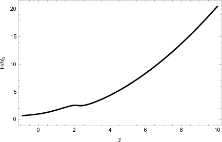
Now let us discuss the results of our numerical analysis and we gather the most characteristic examples of the late-time behavior for the model (2) in Fig. 1, where we plot the statefinder $y_{H}(z)$ (left plot), the total EoS parameter (right plot) and in Fig. 2 the deceleration parameter, as functions of the redshift. Also in Fig. 3 we plot the Hubble rate as a function of the redshift. The behavior of the statefinder $y_{H}(z)$ clearly shows that $y_{H}(z)$ is essentially negative for the whole interval $z=[0,10]$, and this has interesting consequences in view of the observational data reported in Ref. [87], so we comment on the $y_{H}(z)$ behavior in the next section. The behavior of the deceleration parameter can clearly indicate when the Universe is accelerating and when the Universe is decelerating. In our case, the Universe decelerates until $z\sim 2.5$, then it enters an acceleration phase, until $z\sim 1.5$, followed by a decelerating epoch which lasts for nearly 4 billion years until $z\sim 0.5$. After $z\sim 0.5$ the Universe enters the final acceleration era which lasts until present day, nearly 5 billion years. In Fig. 2, we also quote the $\Lambda$CDM behavior of the deceleration parameter (red), and as it can be seen, the $F(R)$ model is indistinguishable from the $\Lambda$CDM model only for the last two billion years approximately, from $z\sim 0.2$ to $z=0$. The same conclusion applies in the behavior of the total EoS parameter in the right plot of Fig. 1, where the red curve represents the behavior of the $\Lambda$CDM model. Thus the $F(R)$ gravity model clearly has two dark energy epochs, one early and one late dark energy epoch, and in between these to dark energy eras, the Universe is decelerating. The same behavior can be verified by looking the right plot of Fig. 1, that is the total EoS parameter for the $F(R)$ gravity model (blue curve), while the red curve corresponds to the $\Lambda$CDM model.

Figure 1: The statefinder function $y_{H}$ for geometric dark energy as a function of the redshift (left plot), and the total EoS parameter $\omega_{tot}$ (right plot).

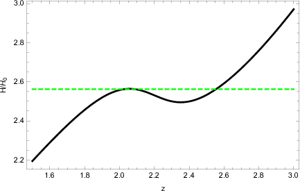
An interesting behavior in the Hubble rate which occurs for $z\sim 2.6$ until $z\sim 2$, is that the Hubble rate at $z\sim 2.2$ has a local minimum, followed by a local maximum at $z\sim 2$ and then the Hubble rate evolves normally to its present day value for the $F(R)$ gravity model. This intriguing behavior is presented in Fig. 3, where we plot $H/H(0)$ as a function of the redshift. The curious behavior is highlighted on the right plot, and it seems that it is an inherent characteristic of the model, we could not attribute this behavior to any other qualitative reasoning. Also we should note that the fraction of the present day value of the Hubble rate for the $F(R)$ gravity model, over the Planck value for the Hubble rate at present day is $\frac{H(0)}{H_{0}}=0.563636$.

Figure 2: The deceleration parameter, as a function of the redshift.

Finally, let us discuss the viability of the $F(R)$ gravity model in a more quantitative way, so let us give the values of the dark energy density parameter $\Omega_{DE}$ and of the dark energy EoS parameter at present day, and we compare these with the Planck 2018 constraints on these quantities. The PYTHON code using the “LSODA” integration technique yields $\omega_{DE}(0)\simeq-0.9961$ which is within the viability limits of the Planck constraint $\omega_{DE}=-1.018\pm 0.031$, and accordingly the dark energy density parameter is found equal to $\Omega_{DE}(0)\simeq 0.6872$, which is an acceptable value when compared to the Planck constraint $\Omega_{DE}=0.6847\pm 0.0073$. Also the deceleration parameter value at present day for the $F(R)$ gravity model is $q(0)\simeq-0.5267$ while for the $\Lambda$CDM model is $q=-0.527$, hence the two values are nearly identical.

A feature of the present $F(R)$ gravity model that is worth mentioning is the fact that the model is free from dark energy oscillations which are known to plague $F(R)$ gravity models for the redshift interval $z=[5,10]$. This in an inherent characteristic of the model as it proves, and thus we may conclude that the occurrence of dark energy oscillations in $F(R)$ gravity models is a model dependent feature.

In conclusion, the $F(R)$ gravity model (2) in the presence of a light axion field, produces a unified phenomenological picture for the inflationary era and the dark energy eras, with the intriguing characteristic of producing actually two distinct dark energy era, one early and one late dark energy eras, with a brief deceleration epoch occurring between these two deceleration eras. Finally let us finally comment that the inverse integration PYTHON code we used and the Mathematica 11 results agree to a great extent.

Figure 3: $\frac{H(z)}{H(0)}$ as a function of the redshift. In the right plot the intriguing behavior of the Hubble rate for redshifts $z\sim 2.6$ until $z\sim 2$ is shown in a more transparent way. The green line in the right plot corresponds to the $H/H(0)$ value $2.56196$.

IV.1 The Behavior at $z\sim 2.34$

Before closing, let us briefly discuss another interesting feature of the model, which is related to the measurement of the Hubble rate at $z=2.34$ reported by [87]. Assuming that the observation is correct, we shall discuss how such an observation is supported by the $F(R)$ gravity model (2). Basically, the observation of [87], indicates that the Hubble rate at redshift $z\sim 2.34$ is $H(z=2.34)=222km/Mpc/sec$, a result which is also discussed in [136, 137, 138, 139]. An interesting way to explain the result of [87], is to make the assumption that $\rho_{DE}<0$ in Eq. (32), since otherwise one would get $\Omega_{m}h^{2}=0.142$ which obviously does not agree with the Cosmic Microwave Background related value of the Planck Collaboration data $\Omega_{c}h^{2}=0.12\pm 0.001$ [81]. Although that a negative dark energy density sounds strange, this concept has appeared in the literature [140, 141]. In our case, negative dark energy density would mean negative values for the statefinder $y_{H}(z)$, and obviously by looking the upper left plot of Fig. 1, we can see that $y_{H}(z)$ is negative for nearly the whole interval $z=[0,10]$. In fact it only becomes positive at $z\sim 1.4$, where it has the value $y_{H}(1.4)=0.227363$ and has the present day value $y_{H}(0)=2.19527$. Let us also comment that negative values of $y_{H}(z)$ in $F(R)$ gravity models frequently occur, since most $f(R)$ gravity models are plagued with dark energy oscillations for the interval $z=[5,10]$ [15, 17]. The present model is free from oscillations though, however $y_{H}$ is negative for nearly the whole interval $z=[0,10]$.

IV.2 The Ghost Issue

Before closing, we need to discuss the important issue of ghosts in the essentially $f(R,\phi)$ theory we discussed in this paper. The ghost instabilities may be developed in a modified gravity theory if the wave speed of the cosmological perturbations, which we will denote as $c_{A}$, is larger than unity. As was shown in Ref. [88] however, for $f(R,\phi)$ theories, the wave speed of the scalar perturbations is unity, thus no ghost instabilities occur in the curvature perturbations. In fact for a flat spacetime, which is our case, the sound speed is equal to the wave speed of the cosmological perturbations (see the last table of Ref. [88]). Let us elaborate on this issue a bit further in order to clarify this important issue. We shall obtain the cosmological perturbations by perturbing the flat FRW metric $g_{\alpha\beta}^{(3)}$ in the following way [88],

$$ds^{2}=-a^{2}(1+\alpha)d\eta^{2}-2\alpha^{2}\beta_{,\alpha}d\eta dx^{\alpha}+a^{2}\left(g_{\alpha\beta}^{(3)}+2\varphi g_{\alpha\beta}^{(3)}+2\gamma_{,\alpha|\beta}+2C_{\alpha\beta}\right)dx^{\alpha}dx^{\beta}\,,$$ (42)

with $g_{\alpha\beta}^{(3)}$ being,

$$g_{\alpha\beta}^{(3)}dx^{\alpha}dx^{\beta}=dr^{2}+r^{2}(d\theta^{2}+\sin^{2}\theta d\phi^{2})\,.$$ (43)

In addition $\eta$ and $a$ in Eq. (42) denote the conformal time and the scale factor. Moreover $\alpha$, $\beta$, $\gamma$ and $\varphi$ in Eq. (42) denote the scalar type order variables of the cosmological perturbations, while the tensor $C_{\alpha\beta}$ stands for the traceless and transverse tensor perturbation. The dynamical evolution of the scalar type perturbation quantified by the variable $\Phi=\varphi_{\delta\phi}$, and which is directly related to the scalar type gauge invariant quantity $\delta\phi_{\varphi}=-\frac{\dot{\phi}}{H}\varphi_{\delta\phi}$, is determined by the differential equation that follows,

$$\frac{\left(H+\frac{\dot{F}_{R}}{2F_{R}}\right)^{2}}{a^{3}\left(\omega\dot{\phi}^{2}+3\frac{(\dot{F}_{R})^{2}}{2F_{R}}\right)}\frac{d}{dt}\left(\frac{a^{3}\left(\omega\dot{\phi}^{2}+3\frac{(\dot{F}_{R})^{2}}{2F_{R}}\right)}{\left(H+\frac{\dot{F}_{R}}{2F_{R}}\right)^{2}}\dot{\Phi}\right)=\frac{\Delta}{a^{2}}\Phi\,,$$ (44)

with $\Delta$ being the Laplacian of the spatial section of the FRW metric. It is apparent from the right hand side of the above evolution equation that the wave speed of the scalar perturbations is equal to unity, thus no ghost instabilities are expected in the cosmological perturbations. But why does the wave speed determines actually whether on not ghost instabilities occur in the first place? Basically, by looking at Eq. (44), the wave speed of the perturbation $\Phi=\varphi_{\delta\phi}$ is equal to unity, but apart from the perturbation $\Phi$ for a general $f(R,\phi)$ theory, there is another scalar perturbation, denoted as $\Psi$, which is defined as follows,

$$\Psi=\varphi_{\chi}+\frac{\dot{F}_{R}}{2F_{R}}\frac{\delta F_{\chi}}{\dot{F}}\,,$$ (45)

the evolution of which is determined by the differential equation that follows,

$$\frac{\omega\dot{\phi}^{2}+3\frac{(\dot{F}_{R})^{2}}{2F}}{\left(H\frac{\dot{F}_{R}}{2F_{R}}\right)(F_{R})}\times$$ (46)

$$\frac{d}{dt}\Big(\frac{\left(H+\frac{\dot{F}_{R}}{2F_{R}}\right)^{2}}{a\left(\omega\dot{\phi}^{2}+3\frac{(\dot{F}_{R})^{2}}{2F_{R}}\right)}\dot{\mathcal{S}}\Big)=\frac{\Delta}{a^{2}}\Psi\,,$$

with the quantity $\mathcal{S}$ being defined below,

$$\mathcal{S}=\frac{a(F_{R})}{H+\frac{\dot{F}_{R}}{2F_{R}}}\Psi\,.$$ (47)

Hence, by looking both Eqs. (44) and (46), which are essentially wave equations, the propagation wave speed is equal to unity, so the wave speed of the propagation of both the fluctuating field and of the perturbed metric is equal to unity. In fact, since the FRW metric we use has a flat spatial part, the sound wave speed defined as $c_{s}^{2}=\frac{\dot{p}}{\dot{\rho}}$ is identical to the wave speed, which is equal to unity. In order to make this more apparent, let us bring both Eqs. (44) and (46) to the Mukhanov-Sasaki form. We define $\bar{z}=c_{A}z$, with $c_{A}=1$ in our case, and $z$ is,

$$z=\frac{a\dot{\phi}}{H}\sqrt{\frac{E}{F_{R}}}\,,$$ (48)

while $E$ is,

$$\centering E=\frac{F_{R}}{\kappa^{2}}\left(1+\frac{3(\dot{F}_{R})^{2}}{2\kappa^{2}\dot{\phi}^{2}F_{R}}\right)\,.\@add@centering$$ (49)

In addition, we introduce $\bar{v}=z\Phi$ and also $u=\frac{a}{\kappa^{2}H}\frac{1}{\bar{z}}\Psi$, hence the wave equations appearing in Eqs. (44) and (46) respectively, can be brought in the well-known Mukhanov-Sasaki forms,

$$\bar{v}^{\prime\prime}-\left(c_{A}^{2}\Delta+\frac{z^{\prime\prime}}{z}\right)\bar{v}=0\,,$$ (50)

$$u^{\prime\prime}-\left(c_{A}^{2}\Delta+\frac{(1/\bar{z})^{\prime\prime}}{1/\bar{z}}\right)u=0\,,$$ (51)

where in our case $c_{A}=1$. Thus the wave speed of the fluctuating fluid and of the perturbed metric is equal to unity, hence no ghost instabilities occur in the theoretical framework we used.

V Concluding Remarks

In this work we investigated the phenomenology of an $F(R)$ gravity model in the presence of a primordial light axion scalar field with broken $U(1)$ Peccei-Quinn symmetry during the inflationary era. Due to the fact that the axion scalar is frozen to its primordial vacuum expectation values, it has a highly subdominant role during the inflationary era, which is predominantly controlled by the $R^{2}$ term of the $F(R)$ gravity. The resulting effective Lagrangian during inflation, has also a rescaled Einstein-Hilbert $R$ term at leading order during inflation. As we demonstrated by performing an explicit calculation, the resulting inflationary phenomenology is identical with that corresponding to the $R^{2}$ model, thus surprisingly the rescaled $R$ term does not affect the dynamical evolution during inflation, at least at leading order. However, if the axion was dynamically evolving during inflation, this result would not be valid. Actually, the rescaled Einstein-Hilbert gravity can significantly affect the inflationary phenomenology of a canonical scalar field as we will show in [131]. After the inflationary era, and specifically when the axion mass $m_{a}$ becomes of the same order as the Hubble rate, and for all cosmic times for which $m_{a}\succeq H$, the axion field starts to oscillate and its energy density evolves as $\rho_{a}\sim a^{-3}$, thus behaves as a dark matter perfect fluid. Accordingly we examined the dark energy phenomenology of the $F(R)$ gravity model in the presence of the axion dark matter perfect fluid and of the radiation perfect fluid. After expressing the Friedmann equation as a function of the redshift and of a suitable statefinder function, we solved numerically the resulting equation, using suitable physically motivated initial conditions corresponding to the late stages of the matter domination era. For the numerical analysis we developed a PYTHON 3 numerical code which is freely available here [80], along with a pedagogical description of the $F(R)$ gravity dark energy phenomenology. The resulting picture is quite interesting phenomenologically, since three novel features for $F(R)$ gravity appear in the theory. Firstly, the Universe experiences an early dark energy era, starting at $z\sim 2.5$ and ending at $z\sim 1.5$, followed by a decelerating epoch which lasts until $z\sim 0.5$, and for the approximately remaining 5 billion years, from $z\sim 0.5$ to $z=0$, the Universe accelerates again. We found that the model is also viable and compatible with the 2018 Planck constraints on the cosmological parameters, at least when the dark energy density parameter and the dark energy EoS parameters are considered. Also the model mimics the $\Lambda$CDM model significantly at the last stages of the evolution prior to present day redshift $z=0$, and at least qualitatively. Secondly, the model is free from dark energy oscillations, which are known to plague the $F(R)$ gravity dark energy phenomenology. Thus our result indicates that the dark energy oscillations might be a model dependent feature of $F(R)$ gravity dark energy phenomenology. Thirdly, the model also complies with the $z\sim 2.34$ observation of [87]. Finally, the model has also another interesting characteristic occurring at $z\sim 2$, where the Hubble rate has a local minimum, followed by a local maximum, after which evolves normally up to $z=0$. This however is another model dependent feature. An interesting phenomenological concept which emerged from the effective Lagrangian of the present $F(R)$ gravity model at early times, is the appearance of a rescaled Einstein-Hilbert term $\alpha R$. Although for the present work, this term played a subdominant term during inflation, due to the presence of the $R^{2}$ term, in conjunction with the fact that the axion scalar was frozen in its vacuum expectation value, it would be interesting to consider the same $F(R)$ gravity model without the $R^{2}$ term, and in the presence of a dynamically evolving canonical scalar field. As we shall show in [131], the results can be quite intriguing in some cases of interest.

Appendix: The Python Code for $F(R)$ Gravity Dark Energy Phenomenology

import numpy as np

import sympy as sp

import matplotlib.pyplot as plt

from scipy.integrate import solve_ivp

 from scipy.integrate import odeint

 from scipy.misc import derivative

#Definition of Hubble rate at present time based on CMB Planck
#2018 data. It is in eV

H0p =
(67.4)*(5.067*10**5*10**13*10**9)/(1.592*1.5637*10**24*10**38)

#Definition of Hubble rate at present time based on Cepheids data.
It is in eV

H0c = (74)*(5.067*10**5*10**13*10**9)/(1.592*1.5637*10**24*10**38)

#Mass scale (eV)

ms = 1.87101*10**(-67)

#Cosmological constant (eV)

Lambda_s= 7.93*1.5*10**(-67)

# the parameter $\chi$, radiation over dark matter present day
energy densities.

chi=3.1*10**(-4)

#The initial redshift value of the redefined redshift z’=0, which
corresponds to the final value of the original redshift z=10

zfin = 0

#initial conditions #Notice that we used the redefined redshift
z’=10-z, so the value zfin=0 of the redefined redshift corresponds
# to zfin=10 of the initial redshift parameter.

r = Lambda_s/(3*ms)*(1 + (11-zfin)/1000)

phi= -Lambda_s/(3*ms)*1/1000

#Model parameters

M = 3.04375*10**22 # in (eV)

#lambda_s=0.01 #dimensionless lambda_s=0.9999 #dimensionless

#t=z from now on in order for the solve_ivp function to work. #Now
you can use fR in your programm

def f(t,y):
    yH=y[0]
    Y=y[1]
    #first definition of the curvature for the numerical integration.
This must be re-defined after the numerical integration
    #in order to be expressed in terms of the new solution
    a=1/(11-t)
    rs=(chi)*a**(-4)
    R=3*ms*((1/a)*Y + 4*yH + a**(-3))
    #The fR and fRR are taken from above
    f=R**2/M**2+lambda_s*R*np.exp(-Lambda_s*5.1/R)+Lambda_s*5.1*lambda_s-(Lambda_s/0.2)*(R/(ms))**0.1
    fR=5.1*Lambda_s*lambda_s*np.exp(-5.1*Lambda_s/R)/R -
0.5*Lambda_s*(R/ms)**0.1/R + lambda_s*np.exp(-5.1*Lambda_s/R) +
2*R/M**2
    fRR=26.01*Lambda_s**2*lambda_s*np.exp(-5.1*Lambda_s/R)/R**3 +
0.45*Lambda_s*(R/ms)**0.1/R**2 + 2/M**2
    #The fR and fRR are taken from above
    J1=a*(-3*fRR - (1/(yH + a**(-3) + rs))*(-fR/(6*ms)))
    J2=(a**2)*(1/(yH + a**(-3) + rs))*(1 - fR)/(3*ms)
    J3=-3*a**(-1)*fRR - ((a**2)*(-fR*(a**(-3) + 2*rs )- f/(3*ms))/(yH
+ a**(-3) + rs))*1/(6*ms)
    #we denote the derivative of y_H with respect to the redefined
redshift z’ as dyHdzr. This is one of the two things
    #that the f function will give us
    dyHdz=Y
    dYdz=-(1/fRR)*(-J1*Y+J2*yH+J3)
    return np.array([dyHdz,dYdz])

# At this point we set the redefined redshift initial and final
#values: from z=0 to z=10. t_span=np.array([0,10])

#And at this point we choose all the intermediate redshift points
#from z=0 to z=10, using 1000 points. In principle one #can choose
#more intermediate points or even less, it is up to the reader.

time_interval=np.linspace(t_span[0],t_span[1],1000)

# Now we set the initial condition. Since y the outcome of the
#solve_ivp that will follow, is an array, with y[0] being the
#function y_H and y[1] being the derivative yH’[z], the initial
#condition is an array fixing the initial value of yH to be r
#defined previously, and that of yH’[z] to be phi, also defined
#previously, below the definition of r.

y0=np.array([r,phi])

# Now we can the solve_ivp function of the scipy module:

soly=solve_ivp(f,t_span,y0,method=’LSODA’,t_eval=time_interval)

# The solution yH is y[0], so we assign the name yH to the
#solution y of the solve_ivp function which we named ’’sol’’ #The
#same with yH’[z] # which we call dotyH

yH=soly.y[0] Y=soly.y[1]

#Now since the above are basically arrays, we switch the redshift
#to the initial definition by using the very own definition # of
#the initial redshift-in our case recall we had to identify z=t in
#order for the solve_ivp function to work.

t=10-soly.t

#Now the definition of the Hubble rate of the present model
#defined as a function of the function yH and of the redshift.
#The outcome is an array, to be #plotted as a function of the
#initially defined redshift which in terms of the programming
#dynamical variable t is t=10-soly.t # look up above this comment.

def a(x):
    return 1/(11-x)

# Now we need to define some functions of the scale factor and of
#the functions yH and dotyH. These must be evaluated for the
#initial time interval, not the redefined t, because the functions
#yH and dotyH were calculated in exactly this way. In the #plots
#we shall make use of the initial redshift values, but in the
#plots we basically connect values of arrays, #a list plot
#basically, so t=10-soly.t is just an array of values. However,
#the functions that will be built depending on yH and #dotyH MUST
#be evaluated using the initial time interval, in our case the
#linspace time_interval

rs=(chi)*a(time_interval)**(-4)

H= np.sqrt(ms*(yH + a(time_interval)**(-3) + rs))

# The derivative of the Hubble rate

dHdz = (ms*(-3*(a(time_interval))**(-2) -
0.00124*a(time_interval)**(-3) + Y))/(2*np.sqrt(ms*(yH +
a(time_interval)**(-3) + rs)))

Omega_Lambda = 0.6847

 Omega_R = 8*10**(-5)

Omega_M = 0.3153 - Omega_R

#Dark energy density parameter

Omega_DE=yH/(yH+ a(time_interval)**(-3) + rs)

#Hubble Rate of LCDM

HLCDM=np.sqrt(H0p**2*(Omega_Lambda+ Omega_M*
a(time_interval)**(-3) + Omega_R*a(time_interval)**(-4)))

#The derivative of the Hubble rate

dHLdz = -(H0p**2*(3*a(time_interval)**(-2)*Omega_M +
4*a(time_interval)**(-3)*Omega_R))/(2*np.sqrt(H0p**2*((a(time_interval))**(-3)*Omega_M+
(a(time_interval))**(-4)*Omega_R + Omega_Lambda)))

#Total Effective Equation of State parameter (Total EoS Parameter)

# For the $F(R)$ gravity model

weff=-1 - 2/3*a(time_interval)**(-1)*dHdz/H

#For the LCDM model

wefflcdm=-1 -2/3*a(time_interval)**(-1)*dHLdz/HLCDM;

#Dark Energy Equation of State Parameter:

wG=-1 -(1/3)*a(time_interval)**(-1)*Y/yH

#DECELERATION Parameter for the F(Rs) Gravity Model

q= -(a(time_interval)**(-1)/H)*dHdz - 1

#DECELERATION for the LCDM Model

qlcdm=-(a(time_interval)**(-1)/HLCDM)*dHLdz - 1

# Now the plots and the results of the numerical analysis # The
#F(R)  model corresponds to blue color, and dashed-dot ’’-.’’
#curve #The LCDM model corresponds to red color and double dashed
#’--’ curve.

#plt.style.use(’Solarize_Light2’)

plt.plot(time_interval,yH,marker=’.’,color=’g’,linestyle=’-.’,label=’Programming
Method’)

plt.plot(t,yH,marker=’.’,color=’b’,linestyle=’--’,label=’Correct
Redshift Method’)

plt.title(’The statefinder $y_H$ vs Redshift’ )

plt.xlabel(’z’) plt.ylabel(’$y_H$’)

plt.tight_layout()

plt.grid(True)

plt.legend()

#plt.savefig(’plot1.eps’)

#plt.savefig(’plot1.jpg’)

plt.show()

plt.plot(time_interval,-Y,marker=’.’,color=’g’,linestyle=’-.’,label=’Programming
Method’)

plt.plot(t,-Y,marker=’.’,color=’b’,linestyle=’--’,label=’Correct
Redshift Method’)

plt.title(’The statefinder derivative $y\’_H$ vs Redshift’ )

plt.xlabel(’z’) plt.ylabel(’$y\’_H$’)

plt.tight_layout()

plt.grid(True)

plt.legend()

#plt.savefig(’dyHp.jpg’)

plt.show()

plt.plot(t,H/H0p,marker=’.’,color=’b’,linestyle=’-.’,label=’$f(R)$’)

plt.plot(t,HLCDM/H0p,marker=’.’,color=’r’,linestyle=’--’,label=’$\Lambda$CDM’)

plt.title(’ $H/H_0$ vs Redshift’ )

plt.xlabel(’z’) plt.ylabel(’Hubble Rates’)

plt.tight_layout()

plt.grid(True)

plt.legend()

#plt.savefig(’Hubblep.jpg’)

plt.show()

Ht=1.996*10**(-33)/H0p*np.ones(1000)

plt.plot(t,H/H0p,marker=’.’,color=’b’,linestyle=’-.’,label=’$f(R)$’)

plt.plot(t,HLCDM/H0p,marker=’.’,color=’r’,linestyle=’--’,label=’$\Lambda$CDM’)

plt.plot(t,Ht,marker=’.’,color=’g’,label=’$H_t=1.996 10^{-33}eV$’)

plt.title(’ $H/H_0$ vs Redshift Close Up’ )

plt.xlabel(’z’) plt.ylabel(’Hubble rates over $H_0$: H/H_0’)

plt.tight_layout()

plt.grid(True)

plt.legend()

#plt.savefig(’Hubblepc.jpg’)

plt.ylim(1, 2) plt.xlim(1.5,3)

plt.show()

plt.plot(t,Omega_DE,marker=’.’,color=’b’,linestyle=’-.’,label=’$\Omega_{DE}(z)$-z
for the f(R) Model’)


plt.title(’$\Omega_{DE}(z)$ vs Redshift’ )


plt.xlabel(’z’) plt.ylabel(’$\Omega_{DE}(z)$’)

plt.tight_layout()

plt.grid(True)

plt.legend()

#plt.savefig(’Omdep.jpg’)

plt.show()

plt.plot(t,weff,marker=’.’,color=’b’,linestyle=’-.’,label=’$\omega_{eff}(z)$-z
for the f(R) Model’)

plt.plot(t,wefflcdm,marker=’.’,color=’r’,linestyle=’--’,label=’$\omega_{eff}(z)$-z
for the $\Lambda$CDM Model’)

plt.title(’Total EoS vs Redshift’)

plt.xlabel(’z’) plt.ylabel(’EoS Parameters’)

plt.tight_layout()

plt.grid(True)

plt.legend()

#plt.savefig(’plot2.eps’)

#plt.savefig(’totaleosp.jpg’)

plt.show()

plt.plot(t,wG,marker=’.’,color=’b’,linestyle=’-.’,label=’$\omega_{DE}(z)$-z
for the f(R) Model’)

plt.title(’Dark Energy EoS vs Redshift’)

plt.xlabel(’z’) plt.ylabel(’EoS Parameters’)

plt.tight_layout()

plt.grid(True)

plt.legend()

#plt.savefig(’odep.jpg’)

plt.show()

plt.plot(t,q,marker=’.’,color=’b’,linestyle=’-.’,label=’$q$-z for
the $f(R)$ Model’)

plt.plot(t,qlcdm,marker=’.’,color=’r’,linestyle=’-.’,label=’$q$-z
for the $\Lambda$CDM Model’)

plt.title(’Deceleration Parameter vs Redshift’)

plt.xlabel(’z’) plt.ylabel(’q’)

plt.tight_layout()

plt.grid(True)

plt.legend()

#plt.savefig(’plot3.eps’)

#plt.savefig(’decelerationp.jpg’)

plt.show()

print("The dark energy density parameter $\Omega_DE(0)$ for the
$f(R)$ Model at present time is:"+" "+str(Omega_DE[999]))
 print()

print()

 print("The dark energy EoS parameter for the $f(R)$ Model
at present time is:"+" "+str(wG[999]))

 print()

  print()

   print("The
Hubble rate for the $f(R)$ Model at present time is:"+"
"+str(H[999]))

print()

print()

 print("The fraction of the Hubble rate for the $f(R)$
Model and of the $\Lmabda$CDM model at present time is:"+"
"+str(H[999]/H0p))

print() print()

print("The deceleration parameter for the $f(R)$ Model at present
time is:"+" "+str(q[999]))

 print()

References

- [1] A. G. Riess et al. [Supernova Search Team], Astron. J. 116 (1998) 1009 [astro-ph/9805201].
- [2] G. Bertone, D. Hooper and J. Silk, Phys. Rept. 405 (2005) 279 doi:10.1016/j.physrep.2004.08.031 [hep-ph/0404175].
- [3] L. Bergstrom, Rept. Prog. Phys. 63 (2000) 793 doi:10.1088/0034-4885/63/5/2r3 [hep-ph/0002126].
- [4] Y. Mambrini, S. Profumo and F. S. Queiroz, Phys. Lett. B 760 (2016) 807 [arXiv:1508.06635 [hep-ph]].
- [5] S. Profumo, arXiv:1301.0952 [hep-ph].
- [6] D. Hooper and S. Profumo, Phys. Rept. 453 (2007) 29 [hep-ph/0701197].
- [7] V. K. Oikonomou, J. D. Vergados and C. C. Moustakidis, Nucl. Phys. B 773 (2007) 19 [hep-ph/0612293].
- [8] S. Nojiri and S. D. Odintsov, Phys. Rev. D 68 (2003) 123512 doi:10.1103/PhysRevD.68.123512 [hep-th/0307288].
- [9] S. Nojiri and S. D. Odintsov, Phys. Lett. B 657 (2007) 238 doi:10.1016/j.physletb.2007.10.027 [arXiv:0707.1941 [hep-th]].
- [10] S. Nojiri and S. D. Odintsov, Phys. Rev. D 77 (2008) 026007 doi:10.1103/PhysRevD.77.026007 [arXiv:0710.1738 [hep-th]].
- [11] G. Cognola, E. Elizalde, S. Nojiri, S. D. Odintsov, L. Sebastiani and S. Zerbini, Phys. Rev. D 77 (2008) 046009 doi:10.1103/PhysRevD.77.046009 [arXiv:0712.4017 [hep-th]].
- [12] S. Nojiri and S. D. Odintsov, Phys. Rev. D 74 (2006) 086005 doi:10.1103/PhysRevD.74.086005 [hep-th/0608008].
- [13] S. A. Appleby and R. A. Battye, Phys. Lett. B 654 (2007) 7 doi:10.1016/j.physletb.2007.08.037 [arXiv:0705.3199 [astro-ph]].
- [14] E. Elizalde, S. Nojiri, S. D. Odintsov, L. Sebastiani and S. Zerbini, Phys. Rev. D 83 (2011) 086006 doi:10.1103/PhysRevD.83.086006 [arXiv:1012.2280 [hep-th]].
- [15] S. D. Odintsov and V. K. Oikonomou, arXiv:2001.06830 [gr-qc].
- [16] P. M. Sá, Phys. Rev. D 102 (2020) no.10, 103519 doi:10.1103/PhysRevD.102.103519 [arXiv:2007.07109 [gr-qc]].
- [17] S. Nojiri, S. D. Odintsov and V. K. Oikonomou, Phys. Rept. 692 (2017) 1 [arXiv:1705.11098 [gr-qc]].
- [18]
S. Capozziello, M. De Laurentis,
Phys. Rept. 509, 167 (2011);
V. Faraoni and S. Capozziello, Fundam. Theor. Phys. 170 (2010). - [19] S. Nojiri, S.D. Odintsov, eConf C0602061, 06 (2006) [Int. J. Geom. Meth. Mod. Phys. 4, 115 (2007)].
- [20] S. Nojiri, S.D. Odintsov, Phys. Rept. 505, 59 (2011);
- [21] A. de la Cruz-Dombriz and D. Saez-Gomez, Entropy 14 (2012) 1717 [arXiv:1207.2663 [gr-qc]].
- [22] G. J. Olmo, Int. J. Mod. Phys. D 20 (2011) 413 [arXiv:1101.3864 [gr-qc]].
- [23] J. Preskill, M. B. Wise and F. Wilczek, Phys. Lett. 120B (1983) 127. doi:10.1016/0370-2693(83)90637-8
- [24] L. F. Abbott and P. Sikivie, Phys. Lett. 120B (1983) 133. doi:10.1016/0370-2693(83)90638-X
- [25] M. Dine and W. Fischler, Phys. Lett. 120B (1983) 137. doi:10.1016/0370-2693(83)90639-1
- [26] D. J. E. Marsh, Phys. Rept. 643 (2016) 1 [arXiv:1510.07633 [astro-ph.CO]].
- [27] P. Sikivie, Lect. Notes Phys. 741 (2008) 19 [astro-ph/0610440].
- [28] G. G. Raffelt, Lect. Notes Phys. 741 (2008) 51 [hep-ph/0611350].
- [29] A. D. Linde, Phys. Lett. B 259 (1991) 38.
- [30] R. T. Co, L. J. Hall and K. Harigaya, Phys. Rev. Lett. 124 (2020) no.25, 251802 doi:10.1103/PhysRevLett.124.251802 [arXiv:1910.14152 [hep-ph]].
- [31] M. C. D. Marsh, H. R. Russell, A. C. Fabian, B. P. McNamara, P. Nulsen and C. S. Reynolds, JCAP 1712 (2017) no.12, 036 [arXiv:1703.07354 [hep-ph]].
- [32] S. D. Odintsov and V. K. Oikonomou, Phys. Rev. D 99 (2019) no.6, 064049 [arXiv:1901.05363 [gr-qc]].
- [33] S. Nojiri, S. D. Odintsov, V. K. Oikonomou and A. A. Popov, Phys. Rev. D 100 (2019) no.8, 084009 [arXiv:1909.01324 [gr-qc]].
- [34] S. Nojiri, S. D. Odintsov and V. K. Oikonomou, Annals Phys. 418 (2020), 168186 doi:10.1016/j.aop.2020.168186 [arXiv:1907.01625 [gr-qc]].
- [35] S. D. Odintsov and V. K. Oikonomou, Phys. Rev. D 99 (2019) no.10, 104070 [arXiv:1905.03496 [gr-qc]].
- [36] M. Cicoli, V. Guidetti and F. G. Pedro, arXiv:1903.01497 [hep-th].
- [37] H. Fukunaga, N. Kitajima and Y. Urakawa, arXiv:1903.02119 [astro-ph.CO].
- [38] A. Caputo, arXiv:1902.02666 [hep-ph].
- [39] A.S.Sakharov and M.Yu.Khlopov, Yadernaya Fizika (1994) V. 57, PP. 514- 516. ( Phys.Atom.Nucl. (1994) V. 57, PP. 485-487); A.S.Sakharov, D.D.Sokoloff and M.Yu.Khlopov, Yadernaya Fizika (1996) V. 59, PP. 1050-1055. (Phys.Atom.Nucl. (1996) V. 59, PP. 1005-1010); M .Yu.Khlopov, A.S.Sakharov and D.D.Sokoloff, Nucl.Phys. B (Proc. Suppl.) (1999) V. 72, 105-109.
- [40] J. H. Chang, R. Essig and S. D. McDermott, JHEP 1809 (2018) 051 [arXiv:1803.00993 [hep-ph]]. Chang:2018rso,Irastorza:2018dyq,
- [41] I. G. Irastorza and J. Redondo, Prog. Part. Nucl. Phys. 102 (2018) 89 [arXiv:1801.08127 [hep-ph]].
- [42] V. Anastassopoulos et al. [CAST Collaboration], Nature Phys. 13 (2017) 584 [arXiv:1705.02290 [hep-ex]].
- [43] P. Sikivie, Phys. Rev. Lett. 113 (2014) no.20, 201301 [arXiv:1409.2806 [hep-ph]].
- [44] P. Sikivie, Phys. Lett. B 695 (2011) 22 [arXiv:1003.2426 [astro-ph.GA]].
- [45] P. Sikivie and Q. Yang, Phys. Rev. Lett. 103 (2009) 111301 [arXiv:0901.1106 [hep-ph]].
- [46] A. Caputo, L. Sberna, M. Frias, D. Blas, P. Pani, L. Shao and W. Yan, Phys. Rev. D 100 (2019) no.6, 063515 [arXiv:1902.02695 [astro-ph.CO]].
- [47] E. Masaki, A. Aoki and J. Soda, arXiv:1909.11470 [hep-ph].
- [48] J. Soda and D. Yoshida, Galaxies 5 (2017) no.4, 96.
- [49] J. Soda and Y. Urakawa, Eur. Phys. J. C 78 (2018) no.9, 779 [arXiv:1710.00305 [astro-ph.CO]].
- [50] A. Aoki and J. Soda, Phys. Rev. D 96 (2017) no.2, 023534 [arXiv:1703.03589 [astro-ph.CO]].
- [51] E. Masaki, A. Aoki and J. Soda, Phys. Rev. D 96 (2017) no.4, 043519 [arXiv:1702.08843 [astro-ph.CO]].
- [52] A. Aoki and J. Soda, Int. J. Mod. Phys. D 26 (2016) no.07, 1750063 [arXiv:1608.05933 [astro-ph.CO]].
- [53] I. Obata and J. Soda, Phys. Rev. D 94 (2016) no.4, 044062 [arXiv:1607.01847 [astro-ph.CO]].
- [54] A. Aoki and J. Soda, Phys. Rev. D 93 (2016) no.8, 083503 [arXiv:1601.03904 [hep-ph]].
- [55] T. Ikeda, R. Brito and V. Cardoso, Phys. Rev. Lett. 122 (2019) no.8, 081101 [arXiv:1811.04950 [gr-qc]].
- [56] A. Arvanitaki, S. Dimopoulos, M. Galanis, L. Lehner, J. O. Thompson and K. Van Tilburg, arXiv:1909.11665 [astro-ph.CO].
- [57] A. Arvanitaki, M. Baryakhtar, S. Dimopoulos, S. Dubovsky and R. Lasenby, Phys. Rev. D 95 (2017) no.4, 043001 [arXiv:1604.03958 [hep-ph]].
- [58] A. Arvanitaki, M. Baryakhtar and X. Huang, Phys. Rev. D 91 (2015) no.8, 084011 [arXiv:1411.2263 [hep-ph]].
- [59] A. Arvanitaki and A. A. Geraci, Phys. Rev. Lett. 113 (2014) no.16, 161801 [arXiv:1403.1290 [hep-ph]].
- [60] S. Sen, Phys. Rev. D 98 (2018) no.10, 103012 [arXiv:1805.06471 [hep-ph]].
- [61] V. Cardoso, S. J. C. Dias, G. S. Hartnett, M. Middleton, P. Pani and J. E. Santos, JCAP 1803 (2018) 043 [arXiv:1801.01420 [gr-qc]].
- [62] J. G. Rosa and T. W. Kephart, Phys. Rev. Lett. 120 (2018) no.23, 231102 [arXiv:1709.06581 [gr-qc]].
- [63] H. Yoshino and H. Kodama, PTEP 2014 (2014) 043E02 [arXiv:1312.2326 [gr-qc]].
- [64] C. S. Machado, W. Ratzinger, P. Schwaller and B. A. Stefanek, arXiv:1912.01007 [hep-ph].
- [65] A. Korochkin, A. Neronov and D. Semikoz, arXiv:1911.13291 [hep-ph].
- [66] A. S. Chou, Astrophys. Space Sci. Proc. 56 (2019) 41.
- [67] C. F. Chang and Y. Cui, arXiv:1911.11885 [hep-ph].
- [68] N. Crisosto, G. Rybka, P. Sikivie, N. S. Sullivan, D. B. Tanner and J. Yang, arXiv:1911.05772 [astro-ph.CO].
- [69] K. Choi, H. Seong and S. Yun, arXiv:1911.00532 [hep-ph].
- [70] M. Kavic, S. L. Liebling, M. Lippert and J. H. Simonetti, arXiv:1910.06977 [astro-ph.HE].
- [71] D. Blas, A. Caputo, M. M. Ivanov and L. Sberna, arXiv:1910.06128 [hep-ph].
- [72] D. Guerra, C. F. B. Macedo and P. Pani, JCAP 1909 (2019) no.09, 061 [arXiv:1909.05515 [gr-qc]].
- [73] T. Tenkanen and L. Visinelli, JCAP 1908 (2019) 033 [arXiv:1906.11837 [astro-ph.CO]].
- [74] G. Y. Huang and S. Zhou, Phys. Rev. D 100 (2019) no.3, 035010 [arXiv:1905.00367 [hep-ph]].
- [75] D. Croon, R. Houtz and V. Sanz, JHEP 1907 (2019) 146 [arXiv:1904.10967 [hep-ph]].
- [76] F. V. Day and J. I. McDonald, JCAP 1910 (2019) no.10, 051 [arXiv:1904.08341 [hep-ph]].
- [77] S. D. Odintsov and V. K. Oikonomou, EPL 129 (2020) no.4, 40001 doi:10.1209/0295-5075/129/40001 [arXiv:2003.06671 [gr-qc]].
- [78] S. Nojiri, S. D. Odintsov, V. K. Oikonomou and A. A. Popov, Phys. Dark Univ. 28 (2020), 100514 doi:10.1016/j.dark.2020.100514 [arXiv:2002.10402 [gr-qc]].
- [79] Y. Akrami et al. [Planck Collaboration], arXiv:1807.06211 [astro-ph.CO].
- [80] https://github.com/VOikonomou?tab=projects
- [81] N. Aghanim et al. [Planck Collaboration], arXiv:1807.06209 [astro-ph.CO].
- [82] M. Doran and G. Robbers, JCAP 0606 (2006) 026 doi:10.1088/1475-7516/2006/06/026 [astro-ph/0601544].
- [83] A. Bhattacharyya and S. Pal, arXiv:1907.10946 [astro-ph.CO].
- [84] J. Sakstein and M. Trodden, arXiv:1911.11760 [astro-ph.CO].
- [85] S. X. Tian, arXiv:1912.13208 [astro-ph.CO].
- [86] S. Nojiri, S. D. Odintsov and V. K. Oikonomou, Phys. Dark Univ. 29 (2020), 100602 doi:10.1016/j.dark.2020.100602 [arXiv:1912.13128 [gr-qc]].
- [87] T. Delubac et al. [BOSS], Astron. Astrophys. 574 (2015), A59 doi:10.1051/0004-6361/201423969 [arXiv:1404.1801 [astro-ph.CO]].
- [88] J. c. Hwang and H. Noh, Phys. Rev. D 71 (2005) 063536 doi:10.1103/PhysRevD.71.063536 [gr-qc/0412126].
- [89] S. Nojiri, S. D. Odintsov and M. Sami, Phys. Rev. D 74 (2006) 046004 doi:10.1103/PhysRevD.74.046004 [hep-th/0605039].
- [90] G. Cognola, E. Elizalde, S. Nojiri, S. Odintsov and S. Zerbini, Phys. Rev. D 75 (2007) 086002 doi:10.1103/PhysRevD.75.086002 [hep-th/0611198].
- [91] S. Nojiri, S. D. Odintsov and M. Sasaki, Phys. Rev. D 71 (2005) 123509 doi:10.1103/PhysRevD.71.123509 [hep-th/0504052].
- [92] S. Nojiri and S. D. Odintsov, Phys. Lett. B 631 (2005) 1 doi:10.1016/j.physletb.2005.10.010 [hep-th/0508049].
- [93] M. Satoh, S. Kanno and J. Soda, Phys. Rev. D 77 (2008) 023526 doi:10.1103/PhysRevD.77.023526 [arXiv:0706.3585 [astro-ph]].
- [94] K. Bamba, A. N. Makarenko, A. N. Myagky and S. D. Odintsov, JCAP 1504 (2015) 001 doi:10.1088/1475-7516/2015/04/001 [arXiv:1411.3852 [hep-th]].
- [95] Z. Yi, Y. Gong and M. Sabir, Phys. Rev. D 98 (2018) no.8, 083521 doi:10.1103/PhysRevD.98.083521 [arXiv:1804.09116 [gr-qc]].
- [96] Z. K. Guo and D. J. Schwarz, Phys. Rev. D 80 (2009) 063523 doi:10.1103/PhysRevD.80.063523 [arXiv:0907.0427 [hep-th]].
- [97] Z. K. Guo and D. J. Schwarz, Phys. Rev. D 81 (2010) 123520 doi:10.1103/PhysRevD.81.123520 [arXiv:1001.1897 [hep-th]].
- [98] P. X. Jiang, J. W. Hu and Z. K. Guo, Phys. Rev. D 88 (2013) 123508 doi:10.1103/PhysRevD.88.123508 [arXiv:1310.5579 [hep-th]].
- [99] P. Kanti, R. Gannouji and N. Dadhich, Phys. Rev. D 92 (2015) no.4, 041302 doi:10.1103/PhysRevD.92.041302 [arXiv:1503.01579 [hep-th]].
- [100] C. van de Bruck, K. Dimopoulos, C. Longden and C. Owen, arXiv:1707.06839 [astro-ph.CO].
- [101] P. Kanti, J. Rizos and K. Tamvakis, Phys. Rev. D 59 (1999) 083512 doi:10.1103/PhysRevD.59.083512 [gr-qc/9806085].
- [102] E. O. Pozdeeva, M. R. Gangopadhyay, M. Sami, A. V. Toporensky and S. Y. Vernov, arXiv:2006.08027 [gr-qc].
- [103] I. Fomin, arXiv:2004.08065 [gr-qc].
- [104] M. De Laurentis, M. Paolella and S. Capozziello, Phys. Rev. D 91 (2015) no.8, 083531 doi:10.1103/PhysRevD.91.083531 [arXiv:1503.04659 [gr-qc]].
- [105] S. Chervon, I. Fomin, V. Yurov and A. Yurov, doi:10.1142/11405
- [106] K. Nozari and N. Rashidi, Phys. Rev. D 95 (2017) no.12, 123518 doi:10.1103/PhysRevD.95.123518 [arXiv:1705.02617 [astro-ph.CO]].
- [107] S. D. Odintsov and V. K. Oikonomou, Phys. Rev. D 98 (2018) no.4, 044039 doi:10.1103/PhysRevD.98.044039 [arXiv:1808.05045 [gr-qc]].
- [108] S. Kawai, M. a. Sakagami and J. Soda, Phys. Lett. B 437, 284 (1998) doi:10.1016/S0370-2693(98)00925-3 [gr-qc/9802033].
- [109] Z. Yi and Y. Gong, Universe 5 (2019) no.9, 200 doi:10.3390/universe5090200 [arXiv:1811.01625 [gr-qc]].
- [110] C. van de Bruck, K. Dimopoulos and C. Longden, Phys. Rev. D 94 (2016) no.2, 023506 doi:10.1103/PhysRevD.94.023506 [arXiv:1605.06350 [astro-ph.CO]].
- [111] B. Kleihaus, J. Kunz and P. Kanti, arXiv:1910.02121 [gr-qc].
- [112] A. Bakopoulos, P. Kanti and N. Pappas, Phys. Rev. D 101 (2020) no.4, 044026 doi:10.1103/PhysRevD.101.044026 [arXiv:1910.14637 [hep-th]].
- [113] K. i. Maeda, N. Ohta and R. Wakebe, Eur. Phys. J. C 72 (2012) 1949 doi:10.1140/epjc/s10052-012-1949-6 [arXiv:1111.3251 [hep-th]].
- [114] A. Bakopoulos, P. Kanti and N. Pappas, arXiv:2003.02473 [hep-th].
- [115] W. Ai, [arXiv:2004.02858 [gr-qc]].
- [116] S. D. Odintsov and V. K. Oikonomou, Phys. Lett. B 797 (2019) 134874 doi:10.1016/j.physletb.2019.134874 [arXiv:1908.07555 [gr-qc]].
- [117] V. K. Oikonomou and F. P. Fronimos, [arXiv:2007.11915 [gr-qc]].
- [118] S. D. Odintsov, V. K. Oikonomou and F. P. Fronimos, Annals Phys. 420 (2020), 168250 doi:10.1016/j.aop.2020.168250 [arXiv:2007.02309 [gr-qc]].
- [119] V. K. Oikonomou and F. P. Fronimos, [arXiv:2006.05512 [gr-qc]].
- [120] S. D. Odintsov and V. K. Oikonomou, Phys. Lett. B 805 (2020), 135437 doi:10.1016/j.physletb.2020.135437 [arXiv:2004.00479 [gr-qc]].
- [121] S. D. Odintsov, V. K. Oikonomou and F. P. Fronimos, [arXiv:2003.13724 [gr-qc]].
- [122] S. D. Odintsov, V. K. Oikonomou, F. P. Fronimos and S. A. Venikoudis, Phys. Dark Univ. 30 (2020), 100718 doi:10.1016/j.dark.2020.100718 [arXiv:2009.06113 [gr-qc]].
- [123] R. Easther and K. i. Maeda, Phys. Rev. D 54 (1996) 7252 doi:10.1103/PhysRevD.54.7252 [hep-th/9605173].
- [124] I. Antoniadis, J. Rizos and K. Tamvakis, Nucl. Phys. B 415 (1994) 497 doi:10.1016/0550-3213(94)90120-1 [hep-th/9305025].
- [125] I. Antoniadis, C. Bachas, J. R. Ellis and D. V. Nanopoulos, Phys. Lett. B 257 (1991), 278-284 doi:10.1016/0370-2693(91)91893-Z
- [126] P. Kanti, N. Mavromatos, J. Rizos, K. Tamvakis and E. Winstanley, Phys. Rev. D 54 (1996), 5049-5058 doi:10.1103/PhysRevD.54.5049 [arXiv:hep-th/9511071 [hep-th]].
- [127] P. Kanti, N. Mavromatos, J. Rizos, K. Tamvakis and E. Winstanley, Phys. Rev. D 57 (1998), 6255-6264 doi:10.1103/PhysRevD.57.6255 [arXiv:hep-th/9703192 [hep-th]].
- [128] S. D. Odintsov, V. K. Oikonomou and F. P. Fronimos, Annals Phys. 424 (2021), 168359 doi:10.1016/j.aop.2020.168359 [arXiv:2011.08680 [gr-qc]].
- [129] S. A. Appleby, R. A. Battye and A. A. Starobinsky, JCAP 06 (2010), 005 doi:10.1088/1475-7516/2010/06/005 [arXiv:0909.1737 [astro-ph.CO]].
- [130] S. D. Odintsov and V. K. Oikonomou, Phys. Lett. B 807 (2020), 135576 doi:10.1016/j.physletb.2020.135576 [arXiv:2005.12804 [gr-qc]].
- [131] V. K. Oikonomou, [arXiv:2012.01312 [gr-qc]].
- [132] W. Hu and I. Sawicki, Phys. Rev. D 76 (2007) 064004 [arXiv:0705.1158 [astro-ph]].
- [133] K. Bamba, A. Lopez-Revelles, R. Myrzakulov, S. D. Odintsov and L. Sebastiani, Class. Quant. Grav. 30 (2013) 015008 [arXiv:1207.1009 [gr-qc]].
- [134] S. D. Odintsov, V. K. Oikonomou, F. P. Fronimos and K. V. Fasoulakos, Phys. Rev. D 102 (2020) no.10, 104042 doi:10.1103/PhysRevD.102.104042 [arXiv:2010.13580 [gr-qc]].
- [135] S. D. Odintsov, V. K. Oikonomou and F. P. Fronimos, Phys. Dark Univ. 29 (2020), 100563 doi:10.1016/j.dark.2020.100563 [arXiv:2004.08884 [gr-qc]].
- [136] M. Moresco et al., JCAP 1605 (2016) 014 doi:10.1088/1475-7516/2016/05/014 [arXiv:1601.01701 [astro-ph.CO]].
- [137] R. Y. Guo and X. Zhang, Eur. Phys. J. C 76 (2016) no.3, 163 doi:10.1140/epjc/s10052-016-4016-x [arXiv:1512.07703 [astro-ph.CO]].
- [138] D. Stern, R. Jimenez, L. Verde, M. Kamionkowski and S. A. Stanford, JCAP 1002 (2010) 008 doi:10.1088/1475-7516/2010/02/008 [arXiv:0907.3149 [astro-ph.CO]].
- [139] C. H. Chuang and Y. Wang, Mon. Not. Roy. Astron. Soc. 435 (2013) 255 doi:10.1093/mnras/stt1290 [arXiv:1209.0210 [astro-ph.CO]].
- [140] M. Ahmed, S. Dodelson, P. B. Greene and R. Sorkin, Phys. Rev. D 69 (2004) 103523 doi:10.1103/PhysRevD.69.103523 [astro-ph/0209274].
- [141] V. H. Cardenas, Phys. Lett. B 750 (2015) 128 doi:10.1016/j.physletb.2015.08.064 [arXiv:1405.5116 [astro-ph.CO]].