Quantum Blackbody Thermometry

Abstract

Blackbody radiation (BBR) sources are calculable radiation sources that are frequently used in radiometry, temperature dissemination, and remote sensing. Despite their ubiquity, blackbody sources and radiometers have a plethora of systematics. We envision a new, primary route to measuring blackbody radiation using ensembles of polarizable quantum systems, such as Rydberg atoms and diatomic molecules. Quantum measurements with these exquisite electric field sensors could enable active feedback, improved design, and, ultimately, lower radiometric and thermal uncertainties of blackbody standards. A portable, calibration-free Rydberg-atom physics package could also complement a variety of classical radiation detector and thermometers. The successful merger of quantum and blackbody-based measurements provides a new, fundamental paradigm for blackbody physics.

I Introduction

In 2019, the International System of Units (SI) was redefined in terms of a set of exact values of physical constants, replacing a system which included reference artifacts. This new system allows anyone, in principle, to perform an identical measurement and arrive at the same value without prior coordination regarding instrumentation. Along with the SI redefinition is a push toward a “quantum SI,” i.e. the ability to realize truly identical metrology by using identical quantum systems which are sensitive to the desired observable via immutable quantum behavior and other fundamental physical laws calculable from first principles.

Blackbodies are incoherent electromagnetic radiation sources that are ubiquitous in radiometry, temperature dissemination, and remote sensing. Blackbody radiation is inherently quantum in nature, as Planck famously hypothesized the quantum nature of light to explain the observed relation between blackbody spectral energy density and wavelength. Using Planck’s law, blackbodies establish a clear relationship between temperature and radiant power. This link allows for the calibration of RF noise, IR imagers, pyrometers, radiation thermometers, and other detectors.

Despite their ubiquity, blackbody sources are susceptible to several systematic errors. In particular, substantial offsets are often observed between measured radiance temperature and temperature measured via contact thermometers [1], with the uncertainty in the offset growing with time from calibration of the contact thermometer. An important challenge is thus to develop a robust alternative to contact thermometers for probing blackbody references, especially for applications which preclude thermometer recalibration, such as remote-sensing satellites. Other systematic effects (e.g., emissivity, propagation loss, temperature gradients, geometric effects, etc.) may be important to blackbody performance as well.

Furthermore, because the detectors blackbodies calibrate are fundamentally classical, these calibrations typically involve undesirably long traceability chains. For example, the International Temperature Scale of 1990 (ITS-90) [2] defines temperatures above 1234.93 K via radiation thermometry. Here, a blackbody acts as a source of radiation which calibrates an optical detector. However, standard BBR thermometers are entirely classical, typically involving an optical system with lenses, a monochromator or other spectral filters, integrating sphere, and detector (such as a photodiode). Each of these classical elements must be carefully characterized in order to accurately measure radiative temperature. For the temperature range 13.8033 K to 1234.93 K, ITS-90 may determine temperature $T_{90}$ by any of 11 different interpolation functions for platinum resistance thermometers which are calibrated at specific defining fixed points; in this important temperature range, both the reference and detector are entirely classical. Furthermore, these fixed point materials, as well as their containment vessels, have stringent purity requirements.

Atoms and molecules are immutable quantum systems whose interactions with electromagnetic radiation have been characterized with exquisite precision and, in many cases, are amenable to ab initio calculation. Atomic transitions already are used explicitly to define the SI second, and implicitly to define all other SI base units apart from the mole. An atom- or molecule-based detector could thus provide internal temperature calibration to a blackbody reference to form a direct, fully quantum-SI realization of radiative temperature.

Blackbody radiation perturbs the internal quantum states of both atoms and molecules. For instance, the BBR-induced Stark shift currently represents the largest, uncompensated systematic in optical clocks [3]. If used as a thermometer, optical clocks can currently measure temperatures to a fractional precision approaching $10^{-5}$ [3]. By choosing a quantum system with a larger polarizability, like a Rydberg atom or a molecule, the Stark shift signal can be increased by a factor of $\sim 10^{3}$ [4, 5].

Figure 1: Fractional temperature sensitivity as a function of temperature. (a) State transfer measurements. Solid lines show population thermalization between $v=0$ and $v=1$ for molecules. Dashed curves show the sensitivity of various $nS$ states of Rb, measuring the transfer to adjacent $P$ levels. Dotted curves show the sensitivity to BBR-induced ionization of Rb from $nS$. (b) Lifetime-limited frequency shift measurements. Solid lines show sensitivity of the $\ket{v=0,N=1}\rightarrow\ket{v=1,N=0}$ transition in molecules, dashed lines show the $5P\rightarrow nS$ transition in Rb.

Here, we consider several quantum measurement approaches using polar molecules and Rydberg atoms to determine the temperature $T$ of the surrounding blackbody radiation. The main results of this work are estimates of the achievable fractional temperature uncertainty $\sqrt{N}\sigma_{T}/T$ of each approach (in this work, $\sigma_{x}$ denote the standard uncertainty in variable $x$), which are summarized in Fig. 1. Assuming $N$ uncorrelated measurements, each measurement approach may potentially achieve $\sqrt{N}\sigma_{T}/T$ of order unity over a wide range of temperatures. Such measurements would constitute direct measurements of thermodynamic temperature in a range currently practically realized under ITS-90 by interpolation between defining fixed points [2] and correction for $T-T_{90}$ [6]. Section II details the interaction of quantum systems with BBR that underpins the thermometric approaches. Section III estimates $\sqrt{N}\sigma_{T}/T$ for laser coolable diatomic molecules from BBR-induced state transfer and level shifts; Section IV applies the same considerations to Rydberg atoms. Sections III and IV also provide experimental considerations relevant to each system. Given the current state of the art, we estimate fractional temperature uncertainty $\sigma_{T}/T\approx 10^{-5}$ could be expected from molecule or Rydberg state transfer measurements or from Rydberg frequency shift measurements. Frequency shift measurements of temperature in molecules are less competitive.

II Blackbody radiation and the two-level system

Planck’s law gives the spectral energy density $U(\omega,T)$ of an ideal blackbody at temperature $T$:

$$U(\omega,T) =\frac{\hbar\omega^{3}}{\pi^{2}c^{3}}\frac{1}{e^{\hbar\omega/k_{\rm{B}}T}-1}$$ (1)

$$=\frac{\hbar\omega^{3}}{\pi^{2}c^{3}}\left<n(\omega)\right>,$$

where $\left<n(\omega)\right>$ is the mean photon number with frequency $\omega$. Due to the narrow linewidths of the molecular vibrational transitions and atomic Rydberg transitions considered here, it is a good approximation to consider each pair of states $\ket{i}$ and $\ket{j}$ interacting with a single, resonant mode of the blackbody with frequency $\omega_{ij}$. In this case, the spontaneous decay rate $\Gamma_{ij}$ is given by

$$\Gamma_{ij}=A_{ij}=\frac{\mu_{ij}^{2}\omega_{ij}^{3}}{3\epsilon_{0}\hbar\pi c^{3}},$$ (2)

and the stimulated rate $\Omega_{ij}$ is given by

$$\Omega_{ij}=B_{ij}U(\omega_{ij},T)=\frac{\mu_{ij}^{2}\omega_{ij}^{3}}{3\epsilon_{0}\hbar\pi c^{3}}\langle n(\omega)\rangle,$$ (3)

where $A_{ij}$ and $B_{ij}$ are the usual Einstein coefficients, and $\mu_{ij}^{2}=\left|\Bra{i}d\ket{j}\right|^{2}$ is the dipole matrix element between states $\ket{i}$ and $\ket{j}$.

Blackbody radiation also shifts the energy of a quantum state $\ket{i}$ by an amount [7]

$$\Delta E_{i}=\frac{1}{6\pi^{2}\epsilon_{0}c^{3}}\sum_{j}P\int_{0}^{\infty}d\omega\frac{\omega^{3}\mu_{ij}^{2}}{e^{\frac{\hbar\omega}{k_{\rm{B}}T}}-1}\left(\frac{2\omega_{ij}}{\omega_{ij}^{2}-\omega^{2}}\right),$$ (4)

with $P$ indicating the Cauchy principal value. Using the Farley-Wing function [7],

$$\mathcal{F}(y)=-2yP\int_{0}^{\infty}dx\frac{x^{3}}{(x^{2}-y^{2})(e^{x}-1)},$$ (5)

Eq. (4) becomes

$$\Delta E_{i}=-\frac{1}{6\pi^{2}\epsilon_{0}c^{3}}\left(\frac{k_{B}T}{\hbar}\right)^{3}\sum_{j}\mu_{ij}^{2}\mathcal{F}\left(\frac{\hbar\omega_{ij}}{k_{B}T}\right).$$ (6)

In the limit where $y\ll 1$, the Farley-Wing function reduces to

$$\mathcal{F}(y)\approx-\frac{\pi^{2}}{3}y.$$ (7)

This limit is important in understanding the asymptotic forms that appear below.

In the following sections, we apply the above equations with generalizations to model the interactions of molecules and Rydberg atoms with BBR.

III Molecules

Cold polar molecules are an emerging quantum technology with great promise for accurately probing BBR. Vanhaecke and Dulieu have considered the state transfer and frequency shifting effects of blackbody radiation on polar molecules for use in precision measurements [8]. Buhmann et al. made similar consideration of the BBR state transfer rates for molecules in proximity to a surface. Here, we interpret the state transfer and frequency shifts in terms of a BBR thermal measurement. Alyabyshev et al. considered using polar molecules to measure applied electric fields [9]. Laser and frequency comb spectroscopy have demonstrated as low as 7 mK precision in measuring the temperature of atmospheric CO₂ [10, 11, 12]. The fractional accuracy $\sigma_{T}/T$ of such measurements in the field is limited to a few $10^{-4}$, however, by uncertainties in abundance and atmospheric pressure.

Diatomic molecules are well suited to probing thermodynamic temperature as their vibrational transition frequencies are typically commensurate with the peak intensity of the blackbody spectrum around room temperature. Several approaches have been developed over the last two decades to produce ultracold trapped molecules [13], including Stark and Zeeman decelerators [14, 15, 16, 17], optoelectric cooling [18], magneto- and photoassociation of ultracold atoms [19, 20, 21, 22], cryogenic buffer gas loading [23, 24], and direct laser cooling [25, 26, 27, 28].

Molecules which may be laser cooled are especially well-suited for BBR thermometry. Unlike most molecules, this class of molecular species has optical cycling transitions, allowing for scattering of potentially millions of optical photons while remaining in one (or a few) quantum states. In the following section, we show that optical cycling transitions may be used to thermalize the molecule population in only the lowest two vibrational levels with the surrounding BBR, enabling sensitive BBR thermometry. Moreover, optical cycling can be used to perform efficient state readout. Recent experiments [28, 29, 30] with laser cooled molecules have demonstrated up to $N\sim 10^{4}$ molecules at temperatures down to $T_{\rm{mol}}\sim 10\,\mu$K. These low temperatures could enable, e.g. a molecule fountain [31, 32] with molecule trajectories entering then exiting the interior of a reference blackbody cavity.

III.1 State Transfer

Previous considerations of BBR on trapped molecules have primarily focused on its effects on trap lifetime [16, 33, 29, 34]. For molecules trapped in the ground vibrational state $v=0$, the relevant timescale for trap loss due to BBR effects is the inverse $v=0\rightarrow v^{\prime}=1$ BBR-induced transition rate $1/\Omega_{01}$. This is consistent with experimental observations: BBR has been reported to limit the trap lifetime for electrostatically trapped OH and OD [16] and magnetically trapped CaF [29]. Furthermore, BBR-induced rotational excitation is an important consideration in molecular ion clocks [34].

Figure 2: Rate equation simulation of free evolution in BBR field of SrF molecules ($v=0-2,N=0-5$, all hyperfine levels included). The state is $\ket{v=0,N=1}$ at time $t\,=\,0$. Solid red, blue, black lines denote the total $v=0,1,2$ populations, respectively. Dashed (dotted) red lines show the $\ket{v=0,N=1}$ ($\ket{v=0,N=3}$) population. Grey lines denote Maxwell-Boltzmann distribution of SrF vibrational levels at $T=300K$.

However, determination of the BBR temperature via population transfer can be done on the faster timescale $t_{\rm{therm}}=1/(\Gamma_{01}+2\Omega_{01})$. This is illustrated in Fig. 2 where we model the SrF system in a 300 K BBR field. We perform rate equation calculations for the populations of a Hund’s case b [35] ground state with total nuclear spin $\bm{I}=1/2$. Included in the simulation are all hyperfine and Zeeman sublevels in vibrational states $v=0-4$ and rotational states $N=0-5$. with population initially in the $\ket{v=0, N^P=1^-,F=2, m_F=2}$ state ($P=\pm$ is the state’s spatial parity, $F$ is the total angular momentum of the system and $m_{F}$ is its projection along the quantization axis). In this case, $1/\Gamma_{01}\approx 0.36$ s, $1/\Omega_{01}\approx 3.7$ s, and $t_{\rm{therm}}\approx 0.33$ s. The total population in each vibrational manifold (solid lines) approaches those predicted by a classical thermodynamic equilibrium (grey lines) after roughly $t_{\rm{therm}}$, while the $\ket{v=0,N=1}$ population (red dashed line) continues to be excited to higher rovibrational states (red dotted line) for time $t~>~t_{\rm{therm}}$.

While the vibrational state populations quickly thermalize in time of order $t_{\rm{therm}}$, within each vibrational manifold the state population will continue to redistribute over a ladder of rotational states $N=0,1,2,\dots$. The continuous excitation to higher rotational states within a vibrational manifold presents a challenge to determining the temperature of the BBR. As the rotational states are typically resolved (e.g. when probed by optical cycling), all significantly populated levels will need to be detected for accurate counting.

Figure 3: Two level thermalization and population measurement scheme for typical laser coolable molecule level structure. (a) Thermalization scheme for molecules initiated in $\ket{X^2\Sigma^+; v=0, N^P=1^-}$. Solid (dashed) black lines denote $P=+$ ($P=-$) states. Solid blue lines denote BBR-induced and spontaneous vibrational transitions, straight arrows denote repump lasers, teal double arrows denote microwave transitions, and wavy arrows denote spontaneous optical decay paths. (b) Method to independently measure the thermalized $v=0$ (red circles) and $v=1$ (blue circles) populations after thermalization scheme (a). i) Four lasers address allowed optical cycling of the thermalized $v=0$ population, allowing population readout by laser induced fluorescence. ii) Microwave $\pi$ pulses are applied to swap the parity $P$ of the thermalized populations. iii) The same four lasers used in step i) now optically cycle and detected the thermalized $v=1$ population. (c) As in (a), but molecules initialized in $\ket{X^2\Sigma^+; v=0, N^P=0^+}$. (d) As in (b), with $v=1$ population probed before $v=0$.

In laser-coolable molecules [25], this issue can be substantially mitigated by virtue of their nearly-diagonal Franck-Condon factors. In Fig. 3a we present a scheme which applies only two lasers and two microwave fields to close the system such that molecules initially in $\ket{X^2\Sigma^+;v=0,N^P=1^-}$ will evolve to only occupy $v=0$ and $v=1$. Laser $\mathcal{L}_{00}^{N=3}$ drives the $\ket{X^2\Sigma^+;v=0,N^P=3^-}\rightarrow\ket{A^2\Pi_{1/2}; v^\prime=0,J^{\prime P}=3/2^+}$ transition, which pumps population into $\ket{X^2\Sigma^+;v=0,N^P=1^-}$ to prevent excitation to states with $N>3$. Microwaves resonant with the transitions between $N=1,2$, and $3$ in the $v=2$ manifold allow transfer to the otherwise unoccupied $\ket{X^2\Sigma^+;v=2,N^P=2^+}$ state; laser $\mathcal{L}_{21}^{N=2}$ then quickly depletes this state by driving the $\ket{X^2\Sigma^+;v=2,N^P=2^+}\rightarrow\ket{A^2\Pi_{1/2}; v^\prime=1,J^{\prime P}=3/2^-}$ transition. The combination of microwaves and laser $\mathcal{L}_{21}^{N=2}$ prevents significant population of states $v\geq 2$. The two-photon microwave plus optical repumping out of $v=2$ ensures molecules will only spontaneously decay to $P=+$ parity $v=1$ levels populated by BBR-induced transitions. All laser and microwave fields are rapidly polarization modulated to destabilize dark $m_{F}$ levels.

The equilibrium population distribution of this scheme has only 2 significantly populated rotational states in each of $v=0,1$. Moreover, population transfer between $v=0,1$ only occurs due to BBR and spontaneous vibrational decay, and does not occur due to the repumping scheme (up to off-diagonal Frank-Condon factors). The populations of excited states, as well as ground states with $v\geq 2$, are roughly $(\Gamma_{01}+\Omega_{01})/\Omega_{\rm{R}}$, where $\Omega_{\rm{R}}$ is the Rabi frequency of the laser coupling to the state. In the limit of sufficient laser and microwave power to saturate the transitions, $\Omega_{\rm{R}}$ is typically $10^{6}$ s^-1 to $10^{7}$ s^-1. and the fractional population outside the effective two level system is less than $10^{-5}$ and can typically be calculated to better than 10 % uncertainty. Thus, the population rapidly approaches a thermal distribution for the $v=0,1$ two-level system at a temperature determined by the surrounding BBR. Figure 3c presents an equivalent two level thermalization scheme for molecules initiated in $\ket{X^2\Sigma^+; v=0, N^P=0^+}$.

Because blackbody radiation is incoherent, it is appropriate to model its interaction with quantum systems with a rate equation model using rates $\Gamma_{ij}$ and $\Omega_{ij}$. We approximate the $v=0,1$ system as a two-level system with energy separation $\hbar\omega_{01}$, state populations $N_{0}$ and $N_{1}$, and total population $N=N_{0}+N_{1}$. Next, we abbreviate $\Omega_{01}=\Omega$ and $\Gamma_{01}=\Gamma$. The state populations evolve according to the rate equations

$$\frac{d}{dt}\begin{pmatrix}N_{0}\\ N_{1}\end{pmatrix}=\begin{pmatrix}-\Omega&\Gamma+\Omega\\ \Omega&-\Gamma-\Omega\end{pmatrix}\begin{pmatrix}N_{0}\\ N_{1}\end{pmatrix}.$$ (8)

If $N_{0}(t=0)=N$ and $N_{1}(t=0)=0$, then the solution is

$$N_{0}(t)=N\left(\frac{\Gamma+\Omega+\Omega e^{-t(\Gamma+2\Omega)}}{\Gamma+2\Omega}\right),$$ (9)

$$N_{1}(t)=N\left(\frac{\Omega(1-e^{-t(\Gamma+2\Omega)})}{\Gamma+2\Omega}\right).$$ (10)

The population evolves toward thermodynamic equilibrium with exponential time constant $t_{\rm{therm}}=1/(\Gamma+2\Omega)$ (in nuclear magnetic resonance notation, $t_{\rm{therm}}=T_{1}$). Using the relation $\Omega/\Gamma=\left<n(\omega_{01})\right>$, we find that the asymptotic behavior is exactly that predicted for a thermal two-level system from quantum statistical mechanics:

$$\frac{N_{1}}{N_{0}}=\frac{\left<n(\omega_{01})\right>}{\left<n(\omega_{01})\right>+1}.$$ (11)

Importantly, the equilibrium state can be calculated from only the temperature $T$ and energy separation $\hbar\omega_{01}$ of the states. Therefore, a population measurement of the two-level system at times which are long compared to $t_{\rm{therm}}$ is a quantum realization of the SI kelvin unit which is traceable to the second. The equilibrium state is independent of the initial state distribution, as well as the experimentally poorly-known transition dipole matrix elements. However, measurement of the population dynamics on timescales comparable to $t_{\rm{therm}}$ in a uniform radiation field (such as a blackbody cavity) would enable the relevant transition dipole matrix element to be determined as well.

For laser-coolable molecules, it should be possible to utilize optical cycling to detect laser-induced fluorescence for independent, shot-noise-limited readout of the $v=0,1$ populations. Typically, optical cycling in molecules primarily occurs by laser $\mathcal{L}_{v,v^{\prime}}=\mathcal{L}_{00}$ driving the $\ket{v=0}\rightarrow\ket{v^\prime=0}$ transition. Molecules decay from $v^{\prime}=0$ to ground vibrational states $v$ with branching fractions $b_{v^{\prime}=0,v}$, and ideally diagonal branching fractions $b_{v,v}\approx 1$. Including $v=0$, the ground vibrational states with the first $k$ largest branching fractions are repumped by additional lasers [25]. If $v=v_{\rm{dark}}$, the vibrational state with the $(k+1)^{\rm{th}}$ largest branching fraction $b_{0,v_{\rm{dark}}}$, is not optically coupled, then roughly $N_{\gamma}=1/b_{0,v_{\rm{dark}}}$ photons may be scattered before the molecule reaches an uncoupled “dark” state. For shot-noise-limited counting, the total photon collection efficiency $\eta$ should be $\eta\gtrsim b_{0,v_{\rm{dark}}}$.

In Fig. 3b,d, we depict an optical cycling scheme coupling $v=0,1$ to readout the state populations after performing the thermalization schemes in Fig.3a,c, respectively. Using SrF as an example, the largest branching fraction to an uncoupled level would be $b_{02}\approx 4\times 10^{-4}$, allowing roughly $N_{\gamma}\approx 2500$ photons to be scattered before optically pumping into a dark vibrational state [36]. The scheme can be generalized to using more repump lasers if necessitated by the branching fractions and detector efficiency.

The standard molecule laser cooling scheme is closed to rotational branching by driving transitions between the first rotationally excited level of the ground electronic state and the lowest rotational level of the excited electronic state [26] (for transitions between two Hund’s case a states, two Hund’s case b states, or a ground Hund’s case b to excited Hund’s case a, the quantum numbers associated with such transitions are $J=1\rightarrow J^{\prime}=0$, $N=1\rightarrow N^{\prime}=0$, or $N=1\rightarrow J^{\prime}=1/2$, respectively). A feature of this optical cycling scheme is that all ground states, including vibrationally excited states, have $P=-$. In contrast, BBR-induced excitation populates successively higher vibrational states with alternating parity (e.g. $P=(-1)^{v+1}$, assuming initial state $\ket{v=0,N^P=1^-}$). Because vibrational excitation from optical cycling and BBR-induced transitions populate states with opposite parity, it is possible to probe the thermalized $v=0,1$ populations independently.

In Fig. 3b step i), optical cycling lasers are applied to first probe the thermalized $v=0$ population. If cycling lasers are applied for a sufficient duration, all $v=0$ molecules scatter roughly $N_{\gamma}$ photons and are optically pumped to dark vibrational levels. In step ii), microwave $\pi$ pulses are applied to swap the parity $P$ of the thermalized populations in $v=0,1$ [29, 28]. In step iii), the optical cycling lasers are reapplied to detect the thermalized $v=1$ population. Figure 3d shows an equivalent population measurement scheme for molecules which thermalize under the scheme of Fig. 3c.

While it was assumed above that the optical cycling lasers are applied for a sufficient period to pump all addressed molecules to a dark state, this need not be the case. If any optically addressed $P=-$ levels remain populated after step i), the $\pi$ pulse of step ii) will transfer the molecule to optically dark $P=+$ levels.

For molecules with hyperfine structure, it may not be possible to perform microwave $\pi$ pulses on every populated hyperfine manifold simultaneously. In this case, steps ii) and iii) may be performed multiple times, with $\pi$ pulses performed on subsets of all hyperfine manifolds at each iteration. Alternately, cycling lasers and microwave could be applied simultaneously to perform steps ii) and iii) at the same time, but might introduce systematic errors in population readout from non-identical cycling schemes for the $v=0$ and $v=1$ populations. Finally, we note that in addition to the BBR temperature measurment outlined below, the thermalization scheme depicted in Fig. 3a,c could be applied to extend the trap lifetime $\tau_{\rm{trap}}$ of conservative molecule traps to exceed $1/\Omega$ [28, 29, 30].

We now assume the $\ket{0}$ and $\ket{1}$ state populations $N_{0}$ and $N_{1}$ can be measured independently, and construct a population asymmetry

$$\mathcal{A}(t)=\frac{N_{0}-N_{1}}{N_{0}+N_{1}}.$$ (12)

For a shot noise-limited measurement, $\sigma_{N_{0}}=\sqrt{N_{0}}$, $\sigma_{N_{1}}=\sqrt{N_{1}}$, and

$$\sigma_{\mathcal{A}}^{2}=\frac{4N_{0}N_{1}}{N^{3}}.$$ (13)

Using Eq. (3) and Eq. (12), we can calculate the temperature uncertainty $\sigma_{T}$

$$\sigma_{T}^{2}=\left(\frac{\partial T}{\partial\Omega}\right)^{2}\left(\frac{\partial\Omega}{\partial\mathcal{A}}\right)^{2}\sigma_{\mathcal{A}}^{2}.$$ (14)

Combining this with Eqs. (2), (3), (9), and (10), and scaling the energy splitting to thermal energy by $x~=~\hbar\omega_{01}/k_{\rm{B}}T$, it is found that the temperature sensitivity of all two-level systems fall on a universal curve (Fig. 1a solid lines) defined only by their transition energy $\hbar\omega_{01}$:

$$\frac{\sigma_{T}}{T}=\sqrt{\frac{(e^{x}+1)^{2}}{e^{x}}}\frac{1}{x}\frac{1}{\sqrt{N}}.$$ (15)

Equation (15) has a minimum fractional temperature uncertainty $\sigma_{T}/T\approx 1.509/\sqrt{N}$ for $x\approx 2.399$, i.e. optimal sensitivity occurs at temperature $T^{*}\approx\hbar\omega_{01}/2.399k_{\rm{B}}$. Moreover, the minimum of Eq. (15) is fairly shallow, with $\sigma_{T}/T$ reaching twice its minimum value at $x\approx 0.704$ and $x\approx 5.674$. Therefore, a single two level system has high sensitivity over a broad range of temperatures by the state transfer method.

	$\nu_{01}$ (cm-1)	$\mu_{01}$ (D)	$\Gamma_{01}$ (s-1)	$\Omega_{01}(T=300\,\rm{K})$ (s-1)	$t_{\rm{therm}}^{T=300\,\rm{K}}$ (s)	$T^{*}$ (K)
BaF	468.9 [37]	0.395 [8]	5.05	0.594	0.160	281
AlCl	481.3 [37]	0.313 [38]	3.42	0.378	0.239	289
YbF	501.91 [37]	0.258 [8]	2.64	0.261	0.316	301
SrF	502.4 [37]	0.264 [39]	2.77	0.272	0.302	301
CaF	581.1 [37]	0.275 [40]	4.65	0.304	0.190	349
MgF	711.69 [37]	0.186 [41]	3.91	0.133	0.240	427
AlF	802.26 [37]	0.235 [38]	8.94	0.195	0.107	481
YO	860.0 [37]	0.297 [42]	17.7	0.289	0.0548	516
BeH	2006.1 [43]	0.094	22.2 [43]	0.0015	0.045	1236
BH	2366.9 [37]	0.088 [44]	32.2	0.0004	0.031	1420

Table 1: Laser-coolable molecules with parameters relevant to BBR thermometry by state transfer.

In principle, any two-level system may use the state-transfer method outlined here to measure the temperature of the surrounding blackbody radiation. Ideally, given some prior knowledge of the range of temperatures likely to be measured, a system should be chosen according to three criteria. First, $\omega_{01}$ should nearly minimize Eq. (15). Second, $\mu_{01}$ should be sufficiently large that $t_{\rm{therm}}$ is short compared to the timescale of a measurement. Third and finally, technical considerations should be given to maximize the number of identical measurements $N$.

In Table 1, we present the relevant vibrational transition parameters to determine $t_{\rm{therm}}$ and $\sigma_{T}/T$ for several laser coolable molecules of interest. Transition dipole matrix elements $\mu_{01}$ are as given in the associated reference, or else calculated using

$$\mu_{v,v+1}=\left(\frac{v+1}{2}\right)^{1/2}\left(\frac{\hbar}{m\omega_{e}}\right)^{1/2}\left[\frac{d\mu}{dR}\right]_{R=R_{e}},$$ (16)

where $\omega_{e}$ is the vibrational frequency, $[d\mu/dR]_{R=R_{e}}$ is the derivative of the dipole moment with bond length $R$, and $m$ is the reduced mass.

Assuming typical $N\approx 10^{4}$ molecules at a repetition rate of $\mathcal{R}=10$ s^-1, temperature sensitivity $\sigma_{T}/T\approx 10^{-4}$ could be achieved in a $t\approx 1$ h, comparable to the time to equilibrate a blackbody cavity with a fixed-point reference. New techniques, such as loading a MOT from a continuous beam [45] or molecule Zeeman slower [46] could enable significantly more trapped molecules to push the measurement sensitivity to $\sigma_{T}/T\approx 10^{-5}$ or lower.

III.2 Frequency Shifts

To first order, the rovibrational energy of a diatomic molecule is given by $\hbar\omega_{v,N}=BN(N+1)+\hbar\omega_{e}(v+1)$, where $B$ is the rotational constant, $\omega_{e}$ is the vibrational constant, $N$ is the rotational quantum number, and $v$ is the vibrational quantum number. In order to understand the relative contributions of the rotational and vibrational structure to the BBR frequency shift, we first consider only the rotational structure, estimating the shifts on rotational state $N$ from all other rotational states. The transition energies between neighboring rotational levels are $\hbar\omega_{N,N-1}=2BN$. Typical rotational constant values are $B\sim h\times 10$ GHz, while $k_{\rm{B}}T\approx h\times 6$ THz for $T=300$ K. Thus, for reasonably small $N$, $x_{N,N^{\prime}}=\hbar\omega_{N,N^{\prime}}/k_{\rm{B}}T\ll 1$ near room temperature, and we can use the approximation of (7). In this limit, the shift is given by

$$\Delta\omega_{N}\approx-\frac{B\mu^{2}}{9\epsilon_{0}\hbar^{2}c^{3}}\left(\frac{k_{B}T}{\hbar}\right)^{2}.$$ (17)

Note that in this model, the BBR shift is independent of rotational state $N$. Therefore, the shifts in neighboring rotational levels cancel (up to non-rigid rotor terms $\sim~DN^{2}(N+1)^{2}$). Measurement of the differential BBR shift between neighboring rotational levels is therefore unlikely to be a generally viable thermometry scheme.

The vibrational transition frequencies $\omega_{v,v^{\prime}}$ in a molecule are generally much closer to the peak of the blackbody spectrum at room temperatures. Inserting (16) into (4) and considering coupling between $v$ and $v^{\prime}=v\pm 1$, we find

$$\Delta\omega_{v}=\frac{1}{6\pi^{2}\epsilon_{0}\hbar c^{3}}\left(\frac{\hbar}{m\omega_{e}}\right)\left[\frac{d\mu}{dR}\right]^{2}_{R=R_{e}}\left(\frac{k_{B}T}{\hbar}\right)^{3}\mathcal{F}\left(\frac{\hbar\omega_{e}}{k_{B}T}\right).$$ (18)

Note that for $v=0$, this expression is also correct even though the only nonzero matrix element is $\mu_{01}$. Much like the rigid rotor example, the harmonic oscillator experiences a state-independent frequency shift up to anharmonic terms.

Nonetheless, we estimate the sensitivity for BeH and MgF from calculated potential energy curves, which implicitly include all anharmonic terms. Eigenenergies and dipole matrix elements $\mu_{ij}$ are taken from the ExoMol line lists for for MgF [41] and BeH [43]. For measurements limited by coherence time $\tau$, the fractional sensitivity to $T$ of a frequency shift measurement is given by

$$\frac{\sigma_{T}}{T}=\frac{1}{T}\left(\frac{\partial T}{\partial\Delta\omega_{v,N,v^{\prime},N^{\prime}}^{\prime}}\right)\frac{1}{\tau},$$ (19)

where $\Delta\omega_{v,N,v^{\prime},N^{\prime}}^{\prime}=\Delta\omega_{v^{\prime},N^{\prime}}-\Delta\omega_{v,N}$ is the differential frequency shift when considering the full rovibrational structure. In Fig. 1b, we evaluate (19) for the $\ket{v=0,N=1}\rightarrow\ket{v^\prime=1,N^\prime=0}$ transition. The coherence time is assumed to be limited by the state lifetime $\tau=1/\gamma_{01}=1/(\Gamma_{01}+\Omega_{01})$, with $\Gamma_{01}$ listed in Table 1 and $\Omega_{01}=\Gamma_{01}\langle n(\nu_{01})\rangle$.

As shown in Fig. 1, the fundamental temperature sensitivity of frequency shift measurements at the coherence time limit may exceed that of the state transfer method at high temperatures. However, it should be noted that achieving lifetime-limited linewidths in molecules at present would be a daunting task. For example, in MgF at $T\approx 600$ K, interrogation for time $\tau\approx 0.2$ s achieves fractional sensitivity $\sigma_{T}/T\approx 1/\sqrt{N}$. This implies a quality factor $Q=\omega/\gamma\approx 10^{13}$, about an order of magnitude higher than has been achieved in a molecular lattice clock [47]. Reaching $10^{-5}$ fractional temperature uncertainty would require controlling systematic frequency shifts at the $10^{-18}$ level, comparable to the best atomic frequency standards. Indeed, existing atomic frequency standards with $10^{-18}$ fractional frequency uncertainty now require thermodynamic temperature measurements with $2\times 10^{-5}$ accuracy [3].

IV Rydberg Atoms

Rydberg atoms offer interesting trade-offs compared to molecules for sensing BBR. Rydberg atoms have transition dipole moments which are three or more orders of magnitude larger than molecules (with interaction strength proportional to the square of the dipole moment). On the other hand, molecules are sensitive to electromagnetic fields in their ground electronic state and thus may gain sensitivity through many orders of magnitude longer interaction time. For Rydberg atoms, the transition dipole matrix elements $\mu_{ij}$ are determined by quantum defect theory at the $\sim$ 1 % level, while there is little experimental data for vibrational transition dipole matrix elements in molecules. Therefore, BBR temperature may be determined by dynamic, as well as equilibrium, population measurements in Rydberg systems.

Rydberg atoms were first used to measure BBR temperature by Hollberg and Hall in 1984 with a roughly 20 % absolute uncertainty [48]. BBR temperature can be determined in Rydberg systems by measuring bound-to-bound [4, 49] or bound-to-continuum [50] transition rates. Ovsiannikov et al. have considered using Rydberg atoms to sense the BBR temperature for more accurate corrections to optical lattice clocks [5].

Significant progress has been made in the development of Rydberg-atom spectroscopic approaches for radio-frequency electric field strength measurements [51, 52, 53, 54, 55, 56, 57, 58]. Rydberg atoms can be used to detect THz radiation, such as thermal radiation. Electromagnetically induced transparency (EIT) is a two-photon process utilized for efficient Rydberg excitation by coupling a ground state to the Rydberg state via an intermediate state. This nonlinear process can also be utilized for THz field sensing. BBR-induced bound-to-bound transition rates may be measured via state-selective electric-field ionization and counting of the field electrons (or ions). Thermal ionization rates may also be measured via photo-electron or ion counting.

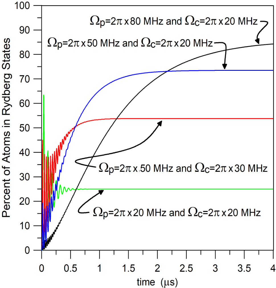
A two-photon excitation scheme has been demonstrated as a simple and efficient method to produce Rb Rydberg atoms. In Rb for example, excitation via $5S_{1/2}\rightarrow 5P_{3/2}\rightarrow nD_{3/2}$ (where $n>15$) may transfer $60~\%$ to $90~\%$ of the resonant atoms to populate the Rydberg state, which is illustrated in Fig. 4. This figure shows the fraction of atoms excited to Rydberg states as a function of time for different $5S_{1/2}\rightarrow P_{3/2}$ laser powers. These results are obtained from the solution of the master equation for the density matrix components of a three-level atomic system discussion in [59].

Figure 4: Rb Rydberg state population for a two-photon excitation. Lines are labeled according to the Rabi frequencies $\Omega_{\rm{p}}$ and $\Omega_{\rm{c}}$ of the probe ($\ket{5S}\rightarrow\ket{5P}$) and coupling ($\ket{5P}\rightarrow\ket{nS}$) transition lasers, respectively.

There are, in principle, three BBR effects on Rydberg atoms that may be considered: level shifts, BBR-induced bound-to-bound transitions, and BBR-induced photo-ionization. The BBR shift of Rydberg levels is only on the order of 10 Hz/K near room temperature. It also tends to be the same for all high-lying Rydberg states, because much of the shift is due to the ponderomotive energy shift of the quasi-free Rydberg electron in the thermal radiation field. In principle one may consider optical measurements of the shifts of individual Rydberg levels, using an auxiliary clock-stabilized Rydberg excitation laser, or a microwave measurement of the transition frequencies between pairs of electric-dipole-coupled Rydberg levels. Microwave measurements of transitions between Rydberg levels would have to be performed at quite low principal quantum numbers ($n\sim 15$), where the thermal Rydberg level shifts become state dependent. In any case, the task would involve measuring transition shifts in the range of 10 mHz to 10 Hz, for Rydberg excitation lines that are 1 kHz or more wide. Assuming that this can be done, one would obtain a calibration-free, atom-based measure of the BBR.

Due to technical and signal-to-noise challenges associated with the level-shift approach, promising alternatives for BBR sensing are to measure BBR-induced Rydberg photoionization rates and Rydberg bound-to-bound transition rates. Thermal ionization rates are in the range of $10^{3}$ s^-1, while bound-to-bound transitions can have rates between $10^{4}$ s^-1 to $10^{5}$ s^-1 , for each final state. Typically, there are on the order of ten final states that become significantly populated. Operating on sample sizes of $10^{6}$ to $10^{10}$ Rydberg atoms, summed over $10^{4}$ to $10^{6}$ experimental cycles acquired at a data rate of about 100 s^-1, we anticipate sufficient statistics to measure temperature to $\sigma_{T}/T\lesssim 10^{-5}$.

IV.1 State Transfer

IV.1.1 Bound-to-bound state transfer

Here we consider measurements involving BBR-induced bound-to-bound state transfer in Rydberg atoms. In these measurements, we excite atoms to an $nS$ Rydberg state using a pulse of the order of 2 $\mu$s, wait a variable time for atoms to evolve in the BBR field, then induce a field-ionization pulse to analyze the transfer of atoms to surrounding $P$ states. Counting the distribution of resulting ions then constitutes a measurement. A benefit of Rydberg atoms is that large numbers of Rydberg atoms ($N\sim 10^{7}$) may be prepared with high repetition rate ($\mathcal{R}\sim 100$ s^-1). For example, a vapor cell with at 60 ^∘C has a Rb density $\approx 3\times 10^{11}$ cm^-3 (the cell may be thermally isolated from the BBR and need not be at the temperature $T$ of the surrounding blackbody). We have confirmed our estimates of $N$ by using a time-domain analysis of the four-level system [59]. We have used this same scheme, with great success, to generate Rydberg atoms for atom-based electric field sensing [51, 52, 53, 54, 55, 56, 57, 58].

We model this interaction by assuming $N$ atoms are initiated in an excited Rydberg state $\ket{0}$. This state has partial spontaneous decay rates $\Gamma_{0j}$, a BBR-stimulated transfer rate $\Omega_{0j}$ from $\ket{0}$ to other, nearby states (generally labeled $\ket{j}$) that we can measure. For concreteness, we will consider the case of $N$ Rb Rydberg atoms in the $nS\equiv\ket{0}$ state at $t=0$. Decay from $nS$ significantly populates several states, with $nP$ and $(n-1)P$ achieving the largest peak populations [60]. We choose to probe the $(n-1)P\equiv\ket{1}$ population dynamics, as it is typically eaisier to resolve from $nS$ than $nP$ through selective ionization. As atoms leave the initially populated $nS$ level, multi-step processes or “cascading” can result in relatively large populations in additional states. Cascading is known to affect the $(n-1)P$ state population dynamics at the 1 % level, and is ignored in the analysis here.

Defining the total depopulation rate of state $\ket{i}$ to be

$$\gamma_{i}=\sum_{j}\left(\Gamma_{ij}+\Omega_{ij}\right),$$ (20)

the population of state $\ket{1}=(n-1)P$ is given by Ref. [60], Eq. (5):

$$N_{1}=N\frac{\Omega_{01}+\Gamma_{01}}{\gamma_{1}-\gamma_{0}}\left(e^{-\gamma_{0}t}-e^{-\gamma_{1}t}\right).$$ (21)

The population $N_{1}$ is maximized at time

$$t^{\text{max}}=\frac{1}{\gamma_{1}-\gamma_{0}}\ln{\frac{\gamma_1}{\gamma_0}}.$$ (22)

Evaluating $N_{1}(t=t^{\rm{max}})$ yields

$$N_{1}^{\text{max}}=N\frac{\Omega_{01}+\Gamma_{01}}{\gamma_{0}}\left(\frac{\gamma_{0}}{\gamma_{1}}\right)^{\frac{\gamma_{1}}{\gamma_{1}-\gamma_{0}}}.$$ (23)

Figure 5 shows $N_{1}$ as a function of time calculated using Eq. (21), with dipole matrix elements and transition energies calculated using the Alkali Rydberg Calculator python package [61, 62]. Unlike the molecule case of Sec III, Rydberg atoms are not closed two level systems, making the timing of the state measurement important. Operationally, given an expected typical temperature $T^{*}$, the population $N_{1}$ should be measured at a various times around the expected maximizing time $t^{\rm{max}*}$. These measurements may then be fit to Eq. (21) in order to determine $\Omega_{01}$, and thus estimate $T$.

We may estimate the sensitivity of this procedure by first noting that it is typically the case in Rydberg systems that $x_{01}=\hbar\omega_{01}/k_{\rm{B}}T\ll 1$. Therefore, using Eq. (3),

$$\Omega_{01}\approx\frac{\mu_{01}^{2}\omega_{01}^{2}}{3\varepsilon_{0}\pi\hbar^{2}c^{3}}k_{\rm{B}}T\equiv aT,$$ (24)

which is linear in temperature.

If we measure the population $N_{1}$ at time $\tau\ll t^{\rm{max}}$, then

$$N_{1} \approx N\Omega_{01}\tau$$ (25)

$$=Na\tau T.$$

We then find

$$\frac{\sigma_{T}}{T}\approx\sqrt{\frac{1}{N_{1}}+\frac{1}{N}}.$$ (26)

While Eq. (25) is not strictly valid at $\tau=t^{\rm{max}}$, we can estimate the optimal sensitivity of the Rydberg state transfer method by substituting $N_{1}=N_{1}^{\rm{max}}$ into Eq  (26). The calculation is shown as dashed lines in Fig. 1 for Rb $nS$ states, with $n=20$ to $n=50$. The fractional temperature sensitivity of this method in the shot noise limit is comparable to the molecule state transfer measurement, with $\sqrt{N}\sigma_{T}/T\approx 4-5$ for a wide range of temperatures $T=100$ K to $T=1300$ K.

Interrogation by two counter-propagating laser beams over a cell length of 2 cm with a $1/e^{2}$ beam diameter 0.5 cm should excite $4\times 10^{7}$ atoms into a Rydberg $nS$ state in a velocity class near the center of the 230 MHz Doppler profile. Of the atoms that are excited, roughly 6 % or $2\times 10^{6}$ atoms will be transferred to an adjacent $P$ state after one state lifetime. Assuming both shot-noise-limited detection and repeating the experiment at $\mathcal{R}=100\,$s^-1, BBR temperatures $T\,\approx\,300$ K may be determined with $\sigma_{T}\approx 100$ mK uncertainty for 1 s of averaging.

Achieving shot noise-limited readout poses a large challenge, given that the ion current is only about 300 fA per pulse. This should be compared with the current require to charge two plates to the necessary electric field strength of 1 kV/cm for inducing the field ionization: for 2 cm $\times$ 1 cm plates separated by 3.5 mm, the capacitance is approximately 0.5 pF. To charge 0.5 pF to 500 V in 10 $\mu$s requires 20 $\mu$A. Thus, the vapor cell needs to control stray electric fields and minimize leakage currents to prevent any contamination of the ion signal. A specialized ammeter capable of separating such large and small currents signals was discussed in Ref. [63].

Figure 5: Rydberg state population transfer dynamics under the three level model.

IV.1.2 Ionization

In this section, we consider BBR-induced bound-to-continuum Rydberg atom transitions, where $N$ atoms initially in state $\ket{0}=nL$ are ionized (i.e. transferred to state $\ket{1}$) at rate $\mathcal{W}$, and decay to all other states $\ket{j}$ at rate $\gamma_{01}$. We use the approximate Eq. (27) derived in Ref. [49], to calculate the ionization rate of an alkali atom,

$$\mathcal{W} =\frac{B_{L}T}{(n-\mu_{L})^{7/3}}\ln{\frac{1}{1-\exp(-\frac{R_\infty}{k_{\rm{B}}T(n-\mu_L)^2})}}$$ (27)

$$\times\Big(\cos(\Delta_L^+ +\frac{\pi}{6})^{2}+\cos(\Delta_L^- -\frac{\pi}{6})^{2}\Big),$$

where $B_{L}=11500A_{L}$ K^-1 s^-1, $A_{L}$ is a scaling coefficient of order unity, $\mu_{L}$ is the quantum defect, $\Delta_{L}^{+}=\pi(\mu_{L}-\mu_{L+1})$, and $\Delta_{L}^{-}=\pi(\mu_{L-1}-\mu_{L})$. Values for these parameters are taken from Refs. [49, 64]. For Rb $nS$ states, we take $A_{L}=1$, $\Delta_{L}^{+}=\pi\times 0.490134$, $\Delta_{L}^{-}=0$, and $\mu_{L}=\mu_{0}+\mu_{2}/(n-\mu_{0})^{2}$, where $\mu_{0}=3.1311804$ and $\mu_{2}=0.1784$.

The state populations are governed by the rate equations

$$\frac{dN_{0}}{dt} =-(\gamma_{0j}+\mathcal{W})N_{0},$$ (28)

$$\frac{dN_{1}}{dt} =\mathcal{W}N_{0},$$

$$\frac{dN_{j}}{dt} =\gamma_{0j}N_{0}.$$

As with the molecule state transfer thermometry method of Sec. IIIA, an advantage of the ionization thermometry method is the atomic population evolves toward an equilibrium distribution. In the $t\rightarrow\infty$ limit,

$$N_{1}=N\frac{\mathcal{W}}{\mathcal{W}+\gamma_{0j}}.$$ (29)

The total number of ions produced is typically $N_{1}/N\approx 0.1$, similar to $N_{1}^{\rm{max}}/N$ in the bound-to-bound method of Sec. IV.1.1. However, the photo-ionization method here requires only a modest guiding field to detect ions with high efficiency. Therefore, achieving the shot noise limit should be less technically challenging than the bound-to-bound state transfer method, which requires $\sim 1$ kV ionizing field for detection. We estimate the temperature sensitivity of BBR-induced ionization in the shot noise limit as

$$\sigma_{T}^{2} =\Big(\frac{\partial T}{\partial\mathcal{W}}\Big)^{2}\left[\Big(\frac{\partial\mathcal{W}}{\partial N_{1}}\Big)^{2}{N_{1}}+\Big(\frac{\partial\mathcal{W}}{\partial N}\Big)^{2}{N}\right]$$ (30)

$$=\Big(\frac{\partial T}{\partial\mathcal{W}}\Big)^{2}\frac{\gamma_{0j}^{2}}{(1-N_{1}/N)^{4}}\frac{N_{1}N+N_{1}^{2}}{N^{2}}\frac{1}{N}$$

$$=\Big(\frac{\partial T}{\partial\mathcal{W}}\Big)^{2}\frac{\mathcal{W}(\mathcal{W}+\gamma_{0j})^{2}(2\mathcal{W}+\gamma_{0j})}{\gamma_{0j}^{2}}\frac{1}{N}.$$

Using Eq. (30), calculated values of $\sqrt{N}\sigma_{T}/T$ for Rb $nS$ states by the ionization method are shown as dotted lines in Fig. 1. The simple three level model outlined here is expected to slightly underestimate the Rydberg ionization temperature sensitivity, as we have ignored BBR induced ionization from other states $\ket{j}$. Bound-to-bound transitions from $nS$ are primarily to states with neighboring principal quantum number $n$, which ionize at a rate of similar order of magnitude to the $nS$ state. By calculating $\mathcal{W}$ with a fuller modeling of the Rydberg population dynamics than Eqs. (28), we expect the error due to the three level approximation in (30) to be $<10$ % at room temperature.

IV.2 Frequency Shifts

Figure 6: BBR shift at $T\,=\,300$ K of Rb Rydberg states as a function of principle quantum number $n$, calculated using Eq. (31).

We consider the energy $\hbar\omega_{nL}$ of state $\ket{nL}$, shifted by the BBR interaction with all other states $\ket{n'L'}$:

$$\Delta\omega_{nL}=-\frac{1}{6\pi^{2}\epsilon_{0}\hbar c^{3}}\left(\frac{k_{B}T}{\hbar}\right)^{3}\sum_{n^{\prime}L^{\prime}}\mu_{nL,n^{\prime}L^{\prime}}^{2}\mathcal{F}\left(\frac{\hbar\omega_{nL,n^{\prime}L^{\prime}}}{k_{B}T}\right),$$ (31)

where $L^{\prime}=L\pm 1$ and $\omega_{nL,n^{\prime}L^{\prime}}=\omega_{n^{\prime}L^{\prime}}-\omega_{nL}$. For large $n$, $\hbar\omega_{nL,n^{\prime}L^{\prime}}/k_{B}T\ll 1$. In this case, using the oscillator sum rule and the approximation of Eq. (7) for $\mathcal{F}(y)$ yields

$$\hbar\Delta\omega_{nL}\approx\frac{\pi}{3}\alpha^{3}\frac{\left(k_{B}T\right)^{2}}{E_{h}},$$ (32)

where $\alpha\,\approx\,1/137$ is the fine structure constant. The shift is proportional to $T^{2}$ and is about 2.4 kHz at $T=300$ K. The shifts for some Rb Rydberg levels are evaluated using Eq. (31) and shown in Fig. 6. For Rb, the shift $\Delta\omega_{nL}$ at room temperature is roughly 1000 times larger in Rydberg states than the $5P$ states. Therefore, the differential shift of the $5P\rightarrow nL$ is essentially equal to $\Delta\omega_{nL}$. The resulting fractional temperature sensitivities to for Rb $nS$ states are shown in Fig. 1b, assuming lifetime-limited interaction time.

While technically more challenging than state transfer, Rydberg frequency shift measurements offer superior sensitivity in the high temperature regime. Moreover, frequency shift thermometry in Rydberg systems appears favorable compared to molecular systems. First, the shifts are larger by roughly three orders of magnitude (e.g. fractional temperature uncertainty of $10^{-5}$ requires only $10^{-15}-10^{-16}$ fractional frequency uncertainty). Having comparable sensitivity $\sqrt{N}\sigma_{T}/T$ to molecules but with relatively short state lifetimes, frequency shift measurements in Rydberg systems may be repeated more rapidly $\mathcal{R}\sim 1000$ s^-1. In this case, with $N=1000$ atoms per measurement, $10^{-5}$ fractional temperature uncertainty could be achieved in $t\sim$1 h averaging time. Frequency measurements of Sr and Yb Rydberg states in an optical lattice at similar sensitivity have been proposed a method for reducing the BBR shift uncertainty in atomic clocks [5].

V Conclusion

The successful implementation of a Rydberg or molecule-based BBR detector would provide an entirely new and direct path to establish primary, quantum-SI-compatible measurements for both radiation and temperature. Development of these techniques is a promising means to correcting BBR frequency shifts in optical clocks [5]. Furthermore, integration of this technology with cold atom miniaturization [65, 66] programs will enable quantum SI radiometry and thermometry to be realized within a single laboratory, or even deployed in a mobile platform. Mobile standards could find several applications, such as on-board primary radiometry calibrations for remote-sensing satellites [67, 68] and high-accuracy non-contact thermometers.

References

- [1] A. C. Carter, R. U. Datla, T. M. Jung, A. W. Smith, and J. A. Fedchak, Low-background temperature calibration of infrared blackbodies, Metrologia 43, S46 (2006).
- [2] H. Preston-Thomas, The international temperature scale of 1990 (ITS-90), Metrologia 27, 3 (1990).
- [3] K. Beloy, N. Hinkley, N. B. Phillips, J. A. Sherman, M. Schioppo, J. Lehman, A. Feldman, L. M. Hanssen, C. W. Oates, and A. D. Ludlow, Atomic clock with room-temperature blackbody stark uncertainty, Phys. Rev. Lett. 113, 260801 (2014).
- [4] H. Figger, G. Leuchs, R. Straubinger, and H. Walther, A photon detector for submillimetre wavelengths using Rydberg atoms, Optics Communications 33, 37 (1980).
- [5] V. D. Ovsiannikov, A. Derevianko, and K. Gibble, Rydberg spectroscopy in an optical lattice: Blackbody thermometry for atomic clocks, Phys. Rev. Lett. 107, 093003 (2011).
- [6] J. Fischer, M. de Podesta, K. D. Hill, M. Moldover, L. Pitre, R. Rusby, P. Steur, O. Tamura, R. White, and L. Wolber, Present estimates of the differences between thermodynamic temperatures and the its-90, International Journal of Thermophysics 32, 12 (2011).
- [7] J. W. Farley and W. H. Wing, Accurate calculation of dynamic stark shifts and depopulation rates of Rydberg energy levels induced by blackbody radiation. hydrogen, helium, and alkali-metal atoms, Phys. Rev. A 23, 2397 (1981).
- [8] N. Vanhaecke and O. Dulieu, Precision measurements with polar molecules: the role of the black body radiation, Molecular Physics 105, 1723 (2007).
- [9] S. V. Alyabyshev, M. Lemeshko, and R. V. Krems, Sensitive imaging of electromagnetic fields with paramagnetic polar molecules, Phys. Rev. A 86, 013409 (2012).
- [10] T. Hieta, M. Merimaa, M. Vainio, J. Seppä, and A. Lassila, High-precision diode-laser-based temperature measurement for air refractive index compensation, Appl. Opt. 50, 5990 (2011).
- [11] L. Gianfrani, Linking the thermodynamic temperature to an optical frequency: recent advances in doppler broadening thermometry, Philosophical Transactions of the Royal Society A: Mathematical, Physical and Engineering Sciences 374, 20150047 (2016).
- [12] A. Hänsel, A. Reyes-Reyes, S. T. Persijn, H. P. Urbach, and N. Bhattacharya, Temperature measurement using frequency comb absorption spectroscopy of CO2, Review of Scientific Instruments 88, 053113 (2017).
- [13] L. Carr, D. DeMille, R. Krems, and J. Ye, Cold and ultracold molecules: science, technology and applications, New J. Phys. 11, 055049 (2009).
- [14] J. R. Bochinski, E. R. Hudson, H. J. Lewandowski, G. Meijer, and J. Ye, Phase space manipulation of cold free radical OH molecules, Phys. Rev. Lett. 91, 243001 (2003).
- [15] S. Y. T. van de Meerakker, P. H. M. Smeets, N. Vanhaecke, R. T. Jongma, and G. Meijer, Deceleration and electrostatic trapping of oh radicals, Phys. Rev. Lett. 94, 023004 (2005).
- [16] S. Hoekstra, J. J. Gilijamse, B. Sartakov, N. Vanhaecke, L. Scharfenberg, S. Y. T. van de Meerakker, and G. Meijer, Optical pumping of trapped neutral molecules by blackbody radiation, Phys. Rev. Lett. 98, 133001 (2007).
- [17] E. Narevicius, A. Libson, C. G. Parthey, I. Chavez, J. Narevicius, U. Even, and M. G. Raizen, Stopping supersonic beams with a series of pulsed electromagnetic coils: An atomic coilgun, Phys. Rev. Lett. 100, 093003 (2008).
- [18] A. Prehn, M. Ibrügger, R. Glöckner, G. Rempe, and M. Zeppenfeld, Optoelectrical cooling of polar molecules to submillikelvin temperatures, Phys. Rev. Lett. 116, 063005 (2016).
- [19] K. Ni, S. Ospelkaus, M. H. G. de Miranda, A. Pe’er, B. Neyenhuis, J. J. Zirbel, S. Kotochigova, P. S. Julienne, D. S. Jin, and J. Ye, A High Phase-Space-Density Gas of Polar Molecules, Science 322, 231 (2008).
- [20] J. G. Danzl, M. J. Mark, E. Haller, M. Gustavsson, R. Hart, J. Aldegunde, J. Hutson, and H.-C. Nägerl, An ultracold high-density sample of rovibronic ground-state molecules in an optical lattice, Nature Physics 6, 265 (2010).
- [21] K. M. Jones, E. Tiesinga, P. D. Lett, and P. S. Julienne, Ultracold photoassociation spectroscopy: Long-range molecules and atomic scattering, Rev. Mod. Phys. 78, 483 (2006).
- [22] S. Stellmer, B. Pasquiou, R. Grimm, and F. Schreck, Creation of Ultracold Molecules in the Electronic Ground State, Phys. Rev. Lett. 109, 115302 (2012).
- [23] J. D. Weinstein, R. deCarvalho, T. Guillet, B. Friedrich, and J. M. Doyle, Magnetic trapping of calcium monohydride molecules at millikelvin temperatures, Nature 395, 148 (1998).
- [24] M. Stoll, J. M. Bakker, T. C. Steimle, G. Meijer, and A. Peters, Cryogenic buffer-gas loading and magnetic trapping of CrH and MnH molecules, Phys. Rev. A 78, 032707 (2008).
- [25] M. D. Di Rosa, Laser-cooling molecules, The European Physical Journal D - Atomic, Molecular, Optical and Plasma Physics 31, 395 (2004).
- [26] B. K. Stuhl, B. C. Sawyer, D. Wang, and J. Ye, Magneto-optical Trap for Polar Molecules, Phys. Rev. Lett. 101, 243002 (2008).
- [27] J. F. Barry, D. J. McCarron, E. N. Norrgard, M. H. Steinecker, and D. DeMille, Magneto-optical trapping of a diatomic molecule, Nature 512, 286 (2014).
- [28] D. J. McCarron, M. H. Steinecker, Y. Zhu, and D. DeMille, Magnetic trapping of an ultracold gas of polar molecules, Phys. Rev. Lett. 121, 013202 (2018).
- [29] H. J. Williams, L. Caldwell, N. J. Fitch, S. Truppe, J. Rodewald, E. A. Hinds, B. E. Sauer, and M. R. Tarbutt, Magnetic trapping and coherent control of laser-cooled molecules, Phys. Rev. Lett. 120, 163201 (2018).
- [30] L. W. Cheuk, L. Anderegg, B. L. Augenbraun, Y. Bao, S. Burchesky, W. Ketterle, and J. M. Doyle, -enhanced imaging of molecules in an optical trap, Phys. Rev. Lett. 121, 083201 (2018).
- [31] M. R. Tarbutt, B. E. Sauer, J. J. Hudson, and E. A. Hinds, Design for a fountain of YbF molecules to measure the electron’s electric dipole moment, New Journal of Physics 15, 053034 (2013).
- [32] C. Cheng, A. P. P. van der Poel, P. Jansen, M. Quintero-Pérez, T. E. Wall, W. Ubachs, and H. L. Bethlem, Molecular fountain, Phys. Rev. Lett. 117, 253201 (2016).
- [33] S. Y. Buhmann, M. R. Tarbutt, S. Scheel, and E. A. Hinds, Surface-induced heating of cold polar molecules, Phys. Rev. A 78, 052901 (2008).
- [34] C. W. Chou, A. L. Collopy, C. Kurz, Y. Lin, M. E. Harding, P. N. Plessow, T. Fortier, S. Diddams, D. Leibfried, and D. R. Leibrandt, Frequency-comb spectroscopy on pure quantum states of a single molecular ion, Science 367, 1458 (2020).
- [35] J. M. Brown and A. Carrington, Rotational spectroscopy of diatomic molecules (Cambridge Univ. Press, 2003).
- [36] J. F. Barry, E. S. Shuman, E. B. Norrgard, and D. DeMille, Laser Radiation Pressure Slowing of a Molecular Beam, Phys. Rev. Lett. 108, 103002 (2012).
- [37] K. P. Huber and G. H. Herzberg, NIST Chemistry WebBook, Constants of Diatomic Molecules, NIST Standard Reference Database Number 69 (National Institute of Standards and Technology, Gaithersburg MD, 20899, 2018).
- [38] M. Yousefi and P. F. Bernath, Line Lists for AlF and AlCl in the X Ground State, The Astrophysical Journal Supplement Series 237, 8 (2018).
- [39] S. R. Langhoff, C. W. Bauschlicher, Jr., H. Partridge, and R. Ahlrichs, Theoretical study of the dipole moments of selected alkaline-earth halides, J. Chem. Phys. 84, 5025 (1986).
- [40] S. Hou and P. F. Bernath, Line list for the ground state of CaF, Journal of Quantitative Spectroscopy and Radiative Transfer 210, 44 (2018).
- [41] S. Hou and P. F. Bernath, Line list for the MgF ground state, Journal of Quantitative Spectroscopy and Radiative Transfer 203, 511 (2017).
- [42] A. N. Smirnov, V. G. Solomonik, S. N. Yurchenko, and J. Tennyson, Spectroscopy of YO from first principles, Phys. Chem. Chem. Phys. 21, 22794 (2019).
- [43] B. Yadin, T. Veness, P. Conti, C. Hill, S. N. Yurchenko, and J. Tennyson, ExoMol line lists – I. The rovibrational spectrum of BeH, MgH and CaH in the X state, Monthly Notices of the Royal Astronomical Society 425, 34 (2012).
- [44] R. J. Blint and W. A. Goddard, The orbital description of the potential energy curves and properties of the lower excited states of the BH molecule, Chemical Physics 3, 297 (1974).
- [45] J. C. Shaw and D. J. McCarron, Bright, continuous beams of cold free radicals, Phys. Rev. A 102, 041302 (2020).
- [46] M. Petzold, P. Kaebert, P. Gersema, M. Siercke, and S. Ospelkaus, A Zeeman slower for diatomic molecules, New Journal of Physics 20, 042001 (2018).
- [47] S. S. Kondov, C.-H. Lee, K. H. Leung, C. Liedl, I. Majewska, R. Moszynski, and T. Zelevinsky, Molecular lattice clock with long vibrational coherence, Nature Physics 15, 1118 (2019).
- [48] L. Hollberg and J. L. Hall, Measurement of the shift of Rydberg energy levels induced by blackbody radiation, Phys. Rev. Lett. 53, 230 (1984).
- [49] I. I. Beterov, D. B. Tretyakov, I. I. Ryabtsev, V. M. Entin, A. Ekers, and N. N. Bezuglov, Ionization of rydberg atoms by blackbody radiation, New Journal of Physics 11, 013052 (2009).
- [50] W. P. Spencer, A. G. Vaidyanathan, D. Kleppner, and T. W. Ducas, Photoionization by blackbody radiation, Phys. Rev. A 26, 1490 (1982).
- [51] C. Holloway, J. Gordon, A. Schwarzkopf, D. Anderson, S. Miller, N. Thaicharoen, and G. Raithel, Broadband Rydberg Atom-Based Electric-Field Probe for SI-Traceable, Self-Calibrated Measurements, IEEE Trans. on Antenna and Propag 62, 6169 (2014).
- [52] C. L. Holloway, M. T. Simons, J. A. Gordon, P. F. Wilson, C. M. Cooke, D. A. Anderson, and G. Raithel, Atom-based rf electric field metrology: From self-calibrated measurements to subwavelength and near-field imaging, IEEE Transactions on Electromagnetic Compatibility 59, 717 (2017).
- [53] J. A. Sedlacek, A. Schwettmann, H. Kübler, R. Löw, T. Pfau, and J. P. Shaffer, Microwave electrometry with Rydberg atoms in a vapour cell using bright atomic resonances, Nature Phys 8, 819 (2012).
- [54] H. Fan, S. Kumar, J. Sedlacek, H. Kübler, S. Karimkashi, and J. P. Shaffer, Atom based RF electric field sensing, Journal of Physics B: Atomic, Molecular and Optical Physics 48, 202001 (2015).
- [55] M. T. Simons, A. H. Haddab, J. A. Gordon, and C. L. Holloway, A Rydberg atom-based mixer: Measuring the phase of a radio frequency wave, Applied Physics Letters 114, 114101 (2019).
- [56] M. T. Simons, A. H. Haddab, J. A. Gordon, D. Novotny, and C. L. Holloway, Embedding a Rydberg Atom-Based Sensor Into an Antenna for Phase and Amplitude Detection of Radio-Frequency Fields and Modulated Signals, IEEE Access 7, 164975 (2019).
- [57] C. L. Holloway, M. T. Simons, J. A. Gordon, and D. Novotny, Detecting and Receiving Phase-Modulated Signals With a Rydberg Atom-Based Receiver, IEEE Antennas and Wireless Propagation Letters 18, 1853 (2019).
- [58] J. A. Gordon, M. T. Simons, A. H. Haddab, and C. L. Holloway, Weak electric-field detection with sub-1 Hz resolution at radio frequencies using a Rydberg atom-based mixer, AIP Advances 9, 045030 (2019).
- [59] C. L. Holloway, M. T. Simons, J. A. Gordon, A. Dienstfrey, D. A. Anderson, and G. Raithel, Electric field metrology for SI traceability: Systematic measurement uncertainties in electromagnetically induced transparency in atomic vapor, Journal of Applied Physics 121, 233106 (2017).
- [60] E. J. Galvez, J. R. Lewis, B. Chaudhuri, J. J. Rasweiler, H. Latvakoski, F. De Zela, E. Massoni, and H. Castillo, Multistep transitions between Rydberg states of Na induced by blackbody radiation, Phys. Rev. A 51, 4010 (1995).
- [61] E. J. Robertson, N. Šibalić, R. M. Potvliege, and M. P. A. Jones, Arc 3.0: An expanded python toolbox for atomic physics calculations (2020), arXiv:2007.12016 [physics.atom-ph] .
- [62] Any mention of commercial products within this work is for information only; it does not imply recommendation or endorsement by NIST, .
- [63] S. Eckel, A. O. Sushkov, and S. K. Lamoreaux, Note: A high dynamic range, linear response transimpedance amplifier, Review of Scientific Instruments 83, 026106 (2012).
- [64] W. Li, I. Mourachko, M. W. Noel, and T. F. Gallagher, Millimeter-wave spectroscopy of cold Rb Rydberg atoms in a magneto-optical trap: Quantum defects of the ns, np, and nd series, Phys. Rev. A 67, 052502 (2003).
- [65] D. Barker, E. Norrgard, N. Klimov, J. Fedchak, J. Scherschligt, and S. Eckel, Single-beam Zeeman slower and magneto-optical trap using a nanofabricated grating, Phys. Rev. Applied 11, 064023 (2019).
- [66] J. P. McGilligan, K. R. Moore, A. Dellis, G. D. Martinez, E. de Clercq, P. F. Griffin, A. S. Arnold, E. Riis, R. Boudot, and J. Kitching, Laser cooling in a chip-scale platform, Applied Physics Letters 117, 054001 (2020).
- [67] D. Gu, D. Houtz, J. Randa, and D. K. Walker, Extraction of illumination efficiency by solely radiometric measurements for improved brightness-temperature characterization of microwave blackbody target, IEEE Transactions on Geoscience and Remote Sensing 50, 4575 (2012).
- [68] R. Datla, M. Weinreb, J. Rice, B. C. Johnson, E. Shirley, and C. Cao, Optical passive sensor calibration for satellite remote sensing and the legacy of NOAA and NIST cooperation, Journal of Research of the National Institute of Standards and Technology 119, 235 (2014).