Optimal Synthesis in a Time-Optimal Problem for the Double Integrator System with a Linear State Constraint

Abstract

We consider a time-optimal problem for the classical “double integrator” system under an arbitrary linear state constraint. Using the maximum principle, we construct the full synthesis of optimal trajectories and provide a qualitative investigation of the measure, the Lagrange multiplier corresponding to the state constraint.

1 Statement of the Problem

On a time interval $[0,T]$ consider the following time-optimal problem:

$$\begin{cases}\begin{aligned} \dot{x}&=y,&\quad x(0)&=x_{0},&\quad x(T)&=0,\\[2.0pt] \dot{y}&=u,&\quad y(0)&=y_{0},&\quad y(T)&=0,\end{aligned}\end{cases}$$ (1)

$$T\to\min,\qquad|u|\leqslant 1,$$ (2)

under a linear state constraint

$$y\,\geqslant\,kx-b\qquad(b>0).$$ (3)

Here $x$ is the position of an object (material point) on a straight line, $y$ its velocity, the control $u$ is an acceleration applied to the object, $t\in[0,T].$ The problem is to move the object from a given initial state $(x_{0},y_{0})$ to the final state $(0,0)$ in the minimum time under the linear constraint (3) on the state variables $x,y.$ We assume that $u(t)$ is an arbitrary measurable bounded function, and hence $x(t),$ $y(t)$ are Lipschitz continuous functions.

In the absence of the state constraint, (1)–(2) is a well-known Feldbaum problem that served as one of the first test examples for application of the Pontryagin maximum principle (see Pont). The case when the constraint (3) is present and $k=0,$ is considered, e.g., in the book IT as an example of application of the maximum principle (MP) in the form of Dubovitskii–Milyutin.  The case of the general constraint (3) has not yet been considered.

Note that (3) is the general form of linear state constraint in this problem which is not vertical. The constraint $y\leqslant kx+b\;\,(b>0)$ is symmetric to this one. The vertical linear constraints $x\leqslant p\,$ and $x\geqslant-p\,\;(p>0)$ will be considered separately in Sec. 6 below.

If either constraint (3) is absent, or is present with $k=0,$ the solution can be found without such an advanced theory as MP, by using just basic tools of calculus. Indeed, here we need to find the minimal time interval on which a Lipschitz function $y(t)$ with given endpoints conditions, the bound on its derivative $|\dot{y}|\leqslant 1,$ and a lower bound on the function itself $y\geqslant-b$ has a given integral. In the absence of this lower bound, we conclude by simple considerations that the optimal function is piecewise linear with the derivative $\pm 1$ and at most one break. If the obtained function violates the lower bound on some time interval, then one must put $y=-b$ on this interval and expand the latter so that the whole function $y(t)$ has the given integral. A detailed elaboration of this solution can be recommended as an exercise for students.

If the restriction (3) is present  and $k\neq 0,$ the solution can hardly be found in the described way, because here the lower bound for the function $y(t)$ at each point $t$ depends on its integral on the interval $[0,t].$ We will apply here the maximum principle for problems with state constraints that was obtained by A.Ya. Dubovitskii and A.A. Milyutin in DM65.

It is well known that the “deciphering” of MP conditions for searching optimal trajectories is not a routine task even for problems without state constraints. The more so this is true if these constraints are present, when both the conditions and their deciphering are more complicated. If we would knew a qualitative structure of optimal trajectories, the search for them could be essentially more simple, but this structure is not a priori known, and we do not impose any assumptions about that. Therefore, we perform here a detailed procedure of solving a problem with a state constraint by means of the MP.  Perhaps it can be useful for solving other problems of this type.

2 Formulation of the Maximum Principle

Let a process $x^{0}(t),y^{0}(t),u^{0}(t),\;t\in[0,T]$ provide the minimum in problem (1)–(3). Assume that its starting point $(x_{0},y_{0})$ does not lie on the state boundary, i.e. $y_{0}>kx_{0}-b.$ (The boundary case will be considered separately.)

Then according to DM65 (see also IT; MDO; develop)  there exist functions of bounded variations $\varphi(t),\,\psi(t)$ (adjoint variables), continuous from the left and not equal both totally zero, nondecreasing function $\mu(t)$ with $\mu(0)=0,$ which generate the Pontryagin function

$$H=\;\varphi y+\psi u$$ (4)

and the augmented Pontryagin function

$$\overline{H}=\;\varphi y+\psi u+\dot{\mu}\left(y-kx+b\right),$$ (5)

so that the following conditions hold: the adjoint (costate) equations

$$\begin{cases}\begin{aligned} \dot{\varphi}&=\,-\overline{H}^{\prime}_{x}&=&\;\;k\dot{\mu},\\[4.0pt] \dot{\psi}&=\,-\overline{H}^{\prime}_{y}&=&\;\,-(\varphi+\dot{\mu}),\end{aligned}\end{cases}$$ (6)

the complementary slackness condition

$$\dot{\mu}(t)\left(y^{0}(t)-kx^{0}(t)+b\right)\,=\,0,$$ (7)

the energy conservation law

$$H(x^{0}(t),y^{0}(t),u^{0}(t))\;\equiv\;\mbox{const}\,\geqslant 0,$$ (8)

and the maximality condition

$$\max_{|u|\leqslant 1}\,H(x^{0}(t),y^{0}(t),u)\;=\;H(x^{0}(t),y^{0}(t),u^{0}(t)).$$

The latter means that

$$u^{0}\,\in\,\Sign\psi\,:=\;\begin{cases}\begin{aligned} +1,\quad&\quad\mbox{ if}\quad\psi>0,\\[4.0pt] -1,\quad&\quad\mbox{ if}\quad\psi<0,\\[4.0pt] [-1,+1],&\quad\mbox{ if}\quad\psi=0.\end{aligned}\end{cases}$$ (9)

Here and thereafter $\dot{\mu}(t)$ is the derivative in the sense of generalized functions. In other words, it is the Radon–Nikodim density of the measure $d\mu(t)$ w.r.t. the Lebesgue measure $dt,$ so the adjoint equations should be understood as equalities between measures, i.e.,

$$d\varphi=\,k\,d{\mu},\qquad d\psi=\,-\varphi\,dt\,-d{\mu},$$

or, in the integral form, for any $t\in[0,T]$

$$\varphi(t+0)-\varphi(0)=\int_{0}^{t+0}k\,d\mu(s),\quad\,\psi(t+0)-\psi(0)=\,-\int_{0}^{t+0}\varphi(s)\,ds-\mu(t+0).$$

The same relates to condition (7), which should be understood as the equality $d\mu(t)\left(y^{0}(t)-kx^{0}(t)+b\right)=0.$ This means that $d\mu(t)$ can be nonzero only on the state boundary, i.e., $d\mu(t)=0$ on any time interval where $y^{0}(t)>kx^{0}(t)+b,$ and so, the costate variables $\psi,\varphi$ are absolutely continuous there.

We do not write the transversality conditions, since the endpoints of trajectory are fixed.  The nontriviality condition means that the case $\varphi\equiv\psi\equiv 0$ is forbidden. In what follows, we drop the superscript 0 for the optimal process.

Before applying the maximum principle, we define the set of starting points from which at least one admissible trajectory originates. This set will be denoted by ${\cal D}$ and called admissible set.  Obviously, it essentially depends on the sign of the coefficient $k.$ It follows from the Filippov theorem that for any initial position from ${\cal D}$ there exists an optimal trajectory.

3 The case $k>0:$ Description of the admissible set

Denote by $\Gamma$ the line $y=kx-b$ (boundary of the admissible state domain), and by $S$ the switching line in the problem without state constraint (we will call it free problem), it is the union of two semi-parabolas: $x=-\frac{1}{2}\,y^{2},\;\;y\geqslant 0\,$ and $x=\frac{1}{2}\,y^{2},\;\;y\leqslant 0.$

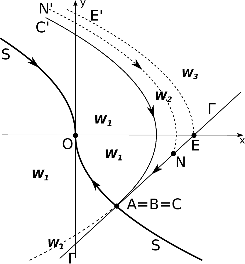
Introduce the following characteristic points for the case $k>0$  (Fig. 1):

1) the point $A$ is the intersection of $\Gamma$ and $S,$

2) the point $E$ is the intersection of $\Gamma$ and the abscissa axis,

3) $C$ is the point where the line $\Gamma$ is tangent to some parabola of the family $x=-\frac{1}{2}\,y^{2}+\mbox{const}\,$ (clearly, this parabola is unique),

4) the point $B$ is the intersection of the tangent parabola from the previous item with the curve $S$.

One can easily find the coordinates of these points. The point $A$ is defined by the relations $x=\frac{1}{2}\,y^{2},\;\;y=kx-b,$ whence

$$x_{A}=\,\frac{(bk+1)-\sqrt{2bk+1}}{k^{2}}\,,\qquad y_{A}=\,\frac{1-\sqrt{2bk+1}}{k}\,.$$

The point $E=(b/k,\,0).$ The point $C$ is common to the parabola $x=-\frac{1}{2}\,y^{2}+m$ and the line $y=kx-b,$ which is tangent to this parabola at $C,$ so $dx/dy=-y=1/k\,.\;$ Hence,

$$y_{C}=\,-\frac{1}{k}\,,\qquad x_{C}=\,\frac{(kb-1)}{k^{2}}\,,\qquad m=\,\frac{2kb-1}{2k^{2}}.$$

The point $B$ is defined by the relations $x=-\frac{1}{2}\,y^{2}+m\;\;x=\frac{1}{2}\,y^{2}\,,$ whence $x_{B}=m/2\,,$ $y_{B}=-\sqrt{m}\,.$ However, we do not need these coordinates for qualitative research, only the relative position of the points $A$ and $C$ on the line $\Gamma$ will be important. Depending on this relative position, there are three possible cases, see Figs. 1, 2 and 3, respectively.

Figure 1: Trajectory $C^{\prime}CBO$ corresponds to the control $u=(-1,\,1),$ trajectory $ABO$ corresponds to $u\equiv 1$

First of all, consider properties of admissible trajectories that are valid in all these three cases.

Let $x(t),\,y(t),\,u(t),\;t\in[0,T]$ be an admissible process. For convenience, we denote by $r(t)=(x(t),\,y(t))$ the state point on the $xOy$ plane. We will say that a point $r=(x,y)\in\Gamma$ lies above (below) a point $r^{\prime}=(x^{\prime},y^{\prime})\in\Gamma$ and write $r>r^{\prime}\,$ if $y>y^{\prime}$ (respectively, $y<y^{\prime}).$

1) The points on the phase boundary that lie below $C$ are never reachable. Indeed, since $y<-1/k$ here, we have $u\geqslant-1>ky,$ so $(y-kx)^{\bullet}=$ $u-ky>0,$ hence we arrive at such a point from the forbidden area, which is impossible.

2) Let $C^{*}$ be the point on the line $\Gamma$ that is the symmetric to $C$ with respect to $E.$ If we got to the state boundary at a point $E_{1}\geqslant C^{*},$ then further motion is impossible, because the dynamics (1) moves us into the forbidden area.  If we got to $\Gamma$ at a point $E_{1}\in(E,C^{*}),$ then further motion is possible only in the lens formed by the line $\Gamma$ and the arc of the parabola coming from the point $E_{1}$ with the control $u=+1,$ and it is impossible to leave this lens obeying the state constraint. Hence, all the points on the state boundary above $E$ are unreachable. It follows that all the points of the upper half-plane lying to the right of parabola $(E^{\prime},E)$ and above $\Gamma$ are also unreachable (because from every such point we would eventually get to the state boundary above the point $E$).

3) An important fact is the following

Lemma 1

An admissible trajectory cannot pass through the point $E.$

Proof.  On the contrary, suppose that $\exists\,t^{\prime}<T$ with $r(t^{\prime})=E,$ that is $x(t^{\prime})=x_{E}$ and $y(t^{\prime})=0.$ Then, for $\bar{x}=x-x_{E}$ and $\tau=t-t^{\prime},$ we have $\dot{\bar{x}}=y$ and $y\geqslant k\bar{x},$ so $\dot{\bar{x}}=k\bar{x}+a(\tau),$ where $a(\tau)\geqslant 0.$ Setting $\bar{x}(\tau)=c(\tau)\,e^{k\tau},$ we obtain $\dot{c}=a(\tau)\,e^{-k\tau}$ and $c(0)=0,$ whence $c(\tau)\geqslant 0$ for all $\tau\geqslant 0.$ Therefore, $\bar{x}(\tau)\geqslant 0$ and $y(\tau)\geqslant k\bar{x}(\tau)\geqslant 0,$ whence $\bar{x}=y=0$ (otherwise we are in the first quadrant and above $\Gamma,$ which is forbidden), so in fact we stay at $E$ until the end and cannot get to the origin. $\Box$

Thus, we cannot reach $E.$ But then we cannot also reach the entire upper part of the parabola $(E^{\prime},E),$ because from there we would get either to $E,$ or to the already forbidden area on the right of this parabola.

4) It follows that the set ${\cal D}$ of initial positions from which there exist admissible trajectories is the half-plane $y\geqslant kx-b$ except the closed set bounded from the left by the parabola $(E^{\prime},E).$ These trajectories consist of motions along the parabolas under the controls $u=-1$ or $u=+1,$ and also motions along the state boundary. Note that ${\cal D}$ is not closed.

5) The state boundary can be reached only on the semi-interval $[C,E),$ and here $\dot{x}=y<0.$ If at some time interval we are on $\Gamma,$ then $y=kx-b,$ $\,\dot{y}=k\dot{x}<0,$ so we can move only in “the left-down” direction from the point $E,$ excluding it, to the point $C.$ Since $u=ky,$ in view of the constraint $|u|\leqslant 1$ this motion can continue only while $|y|\leqslant 1/k\,.$ The limit value $y=-1/k$ corresponds exactly to the point $C.$

4 The case $k>0$:  Analysis of MP 

Let an admissible process $x(t),\,y(t),\,u(t),\;t\in[0,T]$ with a starting point $(x_{0},y_{0})\notin\Gamma$ satisfy the maximum principle. We now pass to its analysis, which for convenience is divided into a number of separate steps.

Lemma 2

If at a time $t^{\prime}$ we are on $\Gamma,$ then $\psi(t^{\prime}-0)\leqslant 0,\,$ $\psi(t^{\prime}+0)\leqslant 0,$ and $\,\Delta\psi(t^{\prime})\leqslant 0.$

If, moreover, $r(t^{\prime})>C,$ then $\Delta\mu(t^{\prime})=0,$ both $\psi$ and $\varphi$ are continuous at $t^{\prime},$ and $\psi(t^{\prime})=0.$

Proof.  In the given case we cannot have $\psi>0$ on the left near $t^{\prime},$ otherwise there would be $u=+1,$ so we came at this point from the forbidden area. Therefore, $\psi(t^{\prime}-0)\leqslant 0.$ By the costate equations, $\Delta\psi(t^{\prime})=-\Delta\mu(t^{\prime})\leqslant 0,$ so $\psi(t^{\prime}+0)\leqslant 0.$

If $r(t^{\prime})>C$ and $\psi(t^{\prime}+0)<0,$ then $\psi<0$ and $u=-1$ in a right neighborhood of $t^{\prime},$ so we penetrate the boundary.  Then $\psi(t^{\prime}+0)\geqslant 0$ and $\Delta\psi(t^{\prime})\geqslant 0.$ But since we already proved $\Delta\psi(t^{\prime})\leqslant 0,$ we get $\Delta\psi(t^{\prime})=0,$ so the measure has no jump, and $\psi(t^{\prime})=0.$ $\Box$

Thus, a jump of measure is possible only at the point $C.$

Lemma 3

If $\psi=0$ on some open interval $\omega=(t^{\prime},t^{\prime\prime}),$ then $\varphi$ is a nonpositive exponential function there.

Proof.    In this case $\dot{\psi}=-(\varphi+\dot{\mu})=0,$ whence $\varphi=-\dot{\mu}\leqslant 0$ and $\dot{\varphi}=k\dot{\mu}=-k\,\varphi,$ hence $\varphi$ is an exponential function on $\omega$. $\Box$

Lemma 4

If on some open interval $(t_{1},t_{2})$ we are on $\Gamma,$ then $\psi=0$ and the measure has a density $\dot{\mu}\geqslant 0$ which is an exponential function. Moreover, $\Delta\mu(t_{1})=0,$ both $\psi$ and $\varphi$ are continuous at $t_{1}\,,$ so they may have jumps only at $t_{2}$.

Proof.    According to Step 5, $u=ky<0$ a.e. on $(t_{1}\,,t_{2}),$ i.e. we move in the “left-down” direction along the interval $(E,C),$ hence $r(t)>C,$ $|y|<1/k\,$ for $t<t_{2}\,,$ so $|u|<1$ and by (9) $\psi=0.$ Then by Lemma 2 $\Delta\mu(t_{1})=0,$ whence by the costate equations $\psi,\,\varphi$ are continuous at $t_{1}\,,$ and by Lemma 3 $\dot{\mu}=-\varphi$ is an exponential function. $\Box$

Lemma 5

The following case is impossible:  $t_{1}<t_{2}\,,$ $r(t_{2})\in\Gamma,$ we are outside of $\Gamma$ for $t<t_{1}$ and $t>t_{2}\,,$ both $\psi$ and $\varphi$ are continuous at $t_{1}$ and vanish on $(t_{1},t_{2}).$

Proof.    In this case $\varphi(t_{1})=\psi(t_{1})=0$ with $\dot{\varphi}=0$ and $\dot{\psi}=-\varphi$ on $[0,t_{1}],$ so we obtain $\varphi=\psi=0$ there, hence also on $[0,t_{2}).$ Let us now see what is on the right of $t_{2}\,.$ If $\Delta\mu(t_{2})=0,$ then $\psi=\varphi=0$ there, hence on the whole $[0,T],$ which is the trivial collection of multipliers. Then $\Delta\mu(t_{2})>0,$ so $r(t_{2})=C,$ moreover $\Delta\varphi(t_{2})>0,$ $\Delta\psi(t_{2})<0,$ and $\dot{\psi}=-\varphi<0$ for $t>t_{2}\,,$ so $\psi<0$ and $u=-1$ for all $t>t_{2}\,.$ But we cannot get to the origin with this control. $\Box$

6) Let $M=\{\,t\;|\;r(t)\in\Gamma\}$ be the set of contact points with the state boundary. If it is empty, the solution is well known — it is the motion along the parabolas of the two above families, see Pont. 

Assume that $M$ is nonempty.  Denote $\,t_{1}=\,\min M,$ $\;t_{2}=\,\max M.$

Lemma 6

$M$ is connected, i.e. is a closed interval or a point: $M=[t_{1},t_{2}].$

Proof.  Suppose on the contrary that $M$ is not connected, i.e. there exist points $t^{\prime}<t^{\prime\prime}$ in $M,$ such that on $\omega=(t^{\prime},t^{\prime\prime})$ we are outside of $\Gamma.$ Then $\dot{\mu}=0$ on $\omega,$ hence $\varphi=\mbox{const}\,,$ and $\psi$ is a linear function.  By Lemma 2, $\psi(t^{\prime}-0)\leqslant 0$ and $\psi(t^{\prime\prime}+0)\leqslant 0.$ If $\psi<0$ on $\omega,$ then $u=-1,$ and we will not get back to $\Gamma$ at $t^{\prime\prime}.\,$ So, $\psi=0$ on $\omega.$

It follows that on any open interval $\omega^{\prime}\subset[t_{1},t_{2}]$ where we are outside of $\Gamma,$ we have $\psi=0$ (since $\omega^{\prime}$ is contained in some maximal interval $\omega$ of the above type), and then, due to the control system, $\varphi=0$ as well. Thus, if on some interval in $[t_{1},t_{2}]$ we have $\psi<0,$ then we are on $\Gamma$ on this interval.

We claim that $\psi=\varphi=0$ on $(t_{1},t_{2}).$ Indeed, suppose $\psi(t_{*})<0$ at some point $t_{*}\in(t_{1},t_{2})$ of its continuity (the case $\psi(t_{*})>0$ is excluded by Lemma 2). Then $\psi<0$ in a neighborhood of this point, so we are on $\Gamma$ and $u=-1.$ But it is impossible to keep on $\Gamma$ with this control. Therefore, $\psi(t)=0$ at all points of its continuity in $(t_{1},t_{2}),$ and hence, everywhere on $(t_{1},t_{2}).\,$ Then by Lemma 3 $\varphi$ is an exponential function. Since $\varphi=0$ on the above interval $\omega,$ we get $\varphi=0$ on $(t_{1},t_{2})$ as well.

Since $\psi(t_{1}+0)=0,$ while by Lemma 2 $\psi(t_{1}-0)\leqslant 0$ and $\Delta\psi(t_{1})\leqslant 0,$ we get $\psi(t_{1}-0)=0,$ so $\Delta\psi(t_{1})=0$ and the functions $\psi,\,\varphi$ are continuous at $t_{1}$ with $\psi(t_{1})=\varphi(t_{1})=0.$ We came to the situation of Lemma 5, which is impossible.

It follows from these arguments that an interval $\omega=(t^{\prime},t^{\prime\prime})$ with the above properties cannot exist, and so $M=[t_{1},t_{2}].$ The lemma is proved. $\Box$

Now, consider all possible cases of location of the set $M.$ This consideration depends on the relative positions of the points $A$ and $C.$

4.1 The case $k>0$ and $C>A$

Define the following closed sets (see Fig. 1):

$\Omega_{1}$ lying on the left of the line $\Gamma$ and the parabola $(C^{\prime},C],$

$\Omega_{2}$ bounded by the parabolas $(C^{\prime},C],\;(E^{\prime},E]$ and the line segment $[C,E],$

and $\Omega_{3}$ lying between the parabola $[E,E^{\prime})$ and the line $\Gamma$.

Recall that domain $\Omega_{3}$ is forbidden, so the set of admissible starting positions ${\cal D}=\,(\Omega_{1}\cup\Omega_{2})\setminus\Omega_{3}$.

7) Can we have $M=\{t_{*}\}$ (touching the boundary at a single point) with $r(t_{*})>C$?  By Lemma 2, there is no jump here, so $\dot{\mu}\equiv 0,$ and the motion is the same as in the free problem, i.e. along the parabolas. But this motion has $u=-1$ in a neighborhood of the point $r(t_{*}),$ then moving from this point we violate the boundary. So, this case is not possible.

8) Can we have $M=[t_{1},t_{2}]$ with $t_{1}<t_{2}$ and $r(t_{2})>C$?  By Lemma 4, in this case there is no jump anywhere, $\psi=0$ and $\dot{\mu}=-\varphi\geqslant 0$ is an exponential function on $M.$ The case $\varphi=0$ is excluded by Lemma 5, so $\varphi<0$ on $M.$

For $t>t_{2}$ the measure switches off, $\varphi=\varphi(t_{2})<0,\,$ $\dot{\psi}=-\varphi>0,$ then $\psi>0,$ $u=+1$ until the end, and we cannot get to the origin with this control from $r(t_{2})>C.$  So, this case is impossible.

9) Suppose that $M=\{t_{*}\}$ and $r(t_{*})=C.$ The first thing that comes to mind in this case is the trajectory $C^{\prime}CBO$ starting at a point $C^{\prime}$ on the parabola $C^{\prime}C$ and having the control $u=(-1,-1,+1).$ Anyway, let us find what the MP implies.

Before and after the point $t_{*}\,,$ the function $\psi$ is linear (in general, with different coefficients), and by Lemma 2 $\psi(t_{*}-0)\leqslant 0$ and $\,\psi(t_{*}+0)\leqslant 0.$  If $\psi(t_{*}+0)=0,$ then $\Delta\mu(t_{*})=0\,$ and $\psi$ is totally linear with $\psi(t_{*})=0.$ The case $\psi\equiv 0$ implies also $\varphi\equiv 0,$ which is forbidden. Then, either $\psi<0,$ $u=-1$ for all $t>t_{*}\,,$ or $\psi>0,$ $u=+1$ there. In both of these cases we do not reach the origin.

Thus, $\psi(t_{*}+0)<0$ and $\psi$ increases on $[t_{*},T]$ (so $\varphi<0$ there) changing its sign from minus to plus at a time $t_{B}\in(t_{*},T)$ corresponding to the point $B,$ with the respective switching of the control from $-1$ to $+1.$ 

Since $\dot{\mu}=0$ both on the left and right of $t_{*}\,,$ then $\Delta\dot{\psi}(t_{*})=-\Delta\varphi(t_{*})\leqslant 0,$ so $\psi$ increases as well on $[0,t_{*})$ up to a value $\psi(t_{*}-0)\leqslant 0,$ hence $\psi<0$ and $u=-1$ on this interval. We thus move along the above trajectory $C^{\prime}CBO.$ Since it is optimal in the free problem, it just occasionally touches the state boundary, which makes no affection on it.

However, let us find a possible value of the jump $\Delta\mu(t_{*}):=\delta$ for this trajectory. Denote by $t_{C}\,,\,t_{B}$ the moments corresponding to the points $C,B$ (here $t_{C}=t_{*}\,).$ Choose the normalization $\dot{\psi}=-\varphi=1$ on $(t_{C},T]$ for our collection of multipliers. Then $\psi=\,t-t_{B}$ on $(t_{C},T]$ independently of $\delta,$ and we should have $\psi(t_{C}-0)=(t_{C}-t_{B})+\delta\leqslant 0,$ whence $0\leqslant\delta\leqslant t_{B}-t_{C}\,.$ For any such $\delta$ we have $\dot{\psi}(t_{C}-0)=-\varphi(t_{C}-0)=1+k\delta>0,$ hence $\psi<0$ on $[0,t_{C}],$ so the MP is satisfied.  Thus, a possible value of the jump of measure at the point $C$ is not unique, being arbitrary within the above bounds. In particular, if $\delta=0,$ then $\psi$ is totally linear. If $\delta=1,$ then $p<0$ on $[0,t_{C}]$ and linearly increases up to the value $\psi(t_{C}-0)=0.$

Thus, the case when $M=\{t_{*}\}$ and $r(t_{*})=C>A$ is completely done.

10) Finally, let $M=[t_{1},t_{2}],$ $t_{1}<t_{2}$ and $r(t_{2})=C.$ Then, by Lemma 4, within $M$ we move along the boundary in the “left-down” direction, the jump at $t_{1}$ is absent, $\psi$ is continuous at this point and vanishes on $[t_{1},t_{2}),$ while $\varphi=-\dot{\mu}\leqslant 0\,$ is an exponential function there.

The case when $\varphi=0$ on $M$ is excluded by Lemma 5, so $\varphi<0$ on $M.$ Moreover, this holds on $[0,t_{1}]$ as well. Then $\dot{\psi}=-\varphi>0,$ so $\psi<0$ and increases up to zero on $[0,t_{1}],$ while $u=-1.$

If the jump at $t_{2}$ is absent, the measure switches off on $[t_{2},T],$ then $\varphi=\mbox{const}\,<0,\,$ $\psi(t_{2})=0$ and $\dot{\psi}=-\varphi>0,$ whence $\psi>0$ and $u=+1$ until the end of motion. Since $r(t_{2})=C>B,$ we cannot get to the origin under this control.

Thus, the measure must have a jump $\Delta\mu(t_{2})=\delta>0.$ Then $\Delta\varphi(t_{2})=k\delta$ and $\psi(t_{2}+0)=-\delta.$ For definiteness, choose the normalization $\dot{\psi}=-\varphi=1$ for $t>t_{2}\,.$ Then $\varphi(t_{2}-0)=-1-k\delta,$ which gives the above relations $\dot{\psi}>0,$ $\psi<0,$ and $u=-1$ on $[0,t_{1}].$ At the switching point $B$ we should have $\psi(t_{B})=-\delta+\Delta t=0,$ where $\Delta t=t_{B}-t_{C}=y_{C}-y_{B}$ is the motion time along the arc $[CB]$ with $u=-1.$ Therefore, $\delta=\,\Delta t.$ For the given positions of the points $C$ and $B$ (which are determined by the value of $k),$ the value of $\Delta t$ is known, so the value of jump $\delta$ is uniquely determined.  So, we have a trajectory of the type $N^{\prime}NCBO$ with $u=(-1,\,ky,\,-1,+1)$ that starts at a point $N^{\prime}\in{\rm int\,}\Omega_{2}\,,$ the first leg of which is the motion with $u=-1$ to a point $N\in(C,E).$

11) Thus, for the case $k>0$ and $C>A,$ we examined all possible cases of location of the set $M$ (the contact set with the state boundary), and for each case we specified the corresponding costate variables and the measure supported on this set.

Since for any starting point in ${\cal D}$ there is only one trajectory satisfying the MP, it is indeed optimal.  This yields the following optimal synthesis.

Theorem 4.1

Let $k>0$ and $C>A$ (Fig. 1). In the domain $\Omega_{1}$ the optimal trajectories are the same as in the free problem.

In the domain ${\rm int\,}\Omega_{2}$ any optimal trajectory is of the type $N^{\prime}NCBO$ with the control $u=(-1,ky,-1,+1)$ and a unique positive jump of measure at the point $B,$ where $N$ is a point on the line interval $(C,E).$

For starting points lying on the interval $(C,E),$ the optimal trajectories are the “tails” of optimal trajectories starting from ${\rm int\,}\Omega_{2}\,,$ the first leg of which is the motion with $u=-1$ to a point on $(C,E).$

4.2 The case $k>0$ and $C=A=B$

Define the following closed sets (see Fig. 2):

$W_{1}$ lying on the left of the line $\Gamma$ and the parabola $(C^{\prime},C],$

$W_{2}$ bounded by the parabolas $(C^{\prime},C],\;(E^{\prime},E]$ and the line segment $[C,E],$

and $W_{3}$ lying between the parabola $[E,E^{\prime})$ and the line $\Gamma$ (forbidden).

Here, the admissible set ${\cal D}=(W_{1}\cup W_{2})\setminus W_{3}\,.$ One can see that Steps 7 and 8 are still valid (see Fig. 2).

12) Consider the case when $M=\{t_{*}\}$ and $r(t_{*})=C.$ Like in Step 9, before and after $t_{*}$ the function $\psi$ is linear (may be, with different coefficients), $\psi(t_{*}-0)\leqslant 0,$ $\,\psi(t_{*}+0)\leqslant 0,\,$ $\Delta\psi(t_{*})\leqslant 0,\,$ and $\Delta\dot{\psi}(t_{*})\leqslant 0.$

If $\Delta\mu(t_{*})>0,$ then $\psi<0$ on the right near $t_{*}\,,$ and further may change its sign to plus, so either $u=-1$ or $u=(-1,+1)$ on $[t_{*},T].$ However, in both these cases we do not reach the origin. Therefore, $\Delta\mu(t_{*})=0,$ whence $\psi$ is totally linear and obviously increases, so $u=(-1,+1)$ on $[0,T]$ with the switching point $t_{*}\,.$ We obtain the trajectory $C^{\prime}CO$ which is optimal in the free problem. It just occasionally touches the state boundary, which makes no affection both on the trajectory and on the costate variables.

Figure 2:

13) Now, let $M=[t_{1},t_{2}],\,$ $t_{1}<t_{2}$ and $r(t_{2})=C.$ Like in Step 10, within $M$ we move along the boundary in the “left-down” direction, $\psi<0$ on $[0,t_{1}]$ and increases up to zero, while $u=-1.$ Further on, $\psi$ is continuous at $t_{1}$ and vanishes on $[t_{1},t_{2});\,$ moreover, $\varphi<0$ on $[0,t_{2}).$

If $\Delta\mu(t_{2})>0,$ then $\psi<0$ on the right near $t_{2}$ and further may change its sign to plus, so either $u=-1$ or $u=(-1,+1)$ on $[t_{2},T].$ But in both these cases we do not reach the origin. Therefore, $\Delta\mu(t_{2})=0$ (the measure is absolutely continuous), hence for $t>t_{2}$ we have $\varphi<0,$ so $\psi>0,$ $u=+1,$ and we obtain the trajectory $N^{\prime}NCO$ with $u=(-1,\,ky,\,+1).$

Thus, for any starting point in ${\cal D},$ a trajectory satisfying the MP is unique, so it is optimal.  Therefore, we obtain

Theorem 4.2

Let $k>0$ and $C=A=B$ (Fig. 2). In the domain $W_{1}$ the optimal trajectories are the same as in the free problem.

In the domain $W_{2}$ an optimal trajectory is of the above type $N^{\prime}NCO$ with $u=(-1,\,ky,\,+1),$ where $N$ is a point on the line interval $(E,C).$

For starting points lying on the interval $(C,E),$ the optimal trajectories are the ”tails”  of optimal trajectories starting from ${\rm int\,}W_{2}\,,$ the first leg of which is the motion with $u=-1$ to a point on $(C,E).$

4.3 The case $k>0\,$ and $C<A$

Define the following closed sets (see Fig. 3):

$Q_{1}$ lying on the left of the line $\Gamma$ and the parabola $(A^{\prime},A],$

$Q_{2}$ bounded by the parabolas $(A^{\prime},A],\;(E^{\prime},E]$ and the line segment $[A,E],$

and $Q_{3}$ lying between the parabola $[E,E^{\prime})$ and the line $\Gamma$ (forbidden).

The admissible set ${\cal D}=(Q_{1}\cup Q_{2})\setminus Q_{3}\,.$ This case differs from the case $C\geqslant A$ in that here the motion along the boundary $\Gamma$ below the point $A$ is of no sense, because one can switch to $u=+1$ at this point and get to the origin in a smaller time.

Therefore, by Lemma 2 the measure has no jumps here altogether. By analogy to Step 7, one can see that the case when $M=\{t_{*}\}$ with $r(t_{2})>A$ is impossible, and by analogy to Step 8, the case when $M=[t_{1},t_{2}]$ with $t_{1}<t_{2}$ and $r(t_{2})>A,$ is also impossible. 

If $M=\{t_{*}\}$ with $r(t_{*})=A,$ the measure is absent by Lemma 2, so we have the trajectory $A^{\prime}AO$ of the free problem.

14) Consider the only possible case with a nonzero measure, which is when $M=[t_{1},t_{2}]$ with $t_{1}<t_{2}$ and $r(t_{2})=A.$ Then, by Lemma 4 $\psi=0$ on $M,$ while by Lemma 5 $\varphi<0$ on $M$ and hence on the whole interval $[0,T].$ Since $\dot{\psi}=-\varphi>0$ both on the left of $t_{1}$ and the right of $t_{2}\,,$ we have $\psi<0,\;\,u=-1$ and $\psi>0,\;\,u=+1$ on these intervals, respectively.  Therefore, we obtain a trajectory $N^{\prime}NAO$ with $u=(-1,\,ky,\,+1),$ where $N$ is a point on the line interval $(E,A).$

Since for any starting point in ${\cal D},$ a trajectory satisfying the MP is unique, it is optimal.  Thus, here the optimal synthesis is as follows.

Figure 3:

Theorem 4.3

Let $k>0$ and $C<A$ (Fig. 3). In the domain $Q_{1}$ the optimal trajectories are the same as in the free problem.

In the domain $Q_{2}$ any optimal trajectory is of the above type $N^{\prime}NAO$ with $u=(-1,\,ky,\,+1),$ where $N$ is a point on the line onterval $(A,E).$

For starting points lying on $(A,E),$ the optimal trajectories are the “tails” of optimal trajectories starting from ${\rm int\,}Q_{2}\,,$ the first leg of which is the motion with $u=-1$ to a point on $(A,E).$

Remark 1.  Note an important property of the Bellman function $V(x_{0},y_{0})$ for the studied problem, that appears in both three subcases for $k>0.$ Recall that it is the minimal time of motion when starting from a point $(x_{0},y_{0}).$ Obviously, $V(x_{0},y_{0})$ is finite for any point in ${\cal D}.$ However, if the point $(x_{0},y_{0})$ tends to boundary parabola $(E^{\prime},E],$ then $V(x_{0},y_{0})\to+\infty.$ This is caused by the fact that if $(x_{0},y_{0})$ is close to that parabola, then at some moment $t_{*}$ the corresponding optimal trajectory gets to a point $r(t_{*})$ of the interval $(C,E)$ and then goes along this interval up to the point $C$ or $A.$ Since the latter motion obeys $\dot{y}=ky,$ the time of motion along the interval $[r(t_{*}),C]$ or $[r(t_{*}),A]$ tends to infinity as $r(t_{*})$ tends to $E.$

5 The case $k<0$

Denote $k=-q,$ where $q>0.$ The boundary $\Gamma$ of the admissible state domain is now defined by $y=-qx-b,$ while the switching line $S$ is the same as before. There are three qualitative different cases here, depending on the number of points where the line $\Gamma$ and the curve $S$ intersect:  one, two, or three.

5.1 The case $k<0$ with three intersection points

Introduce characteristic points for this case. Let $C$ be the point where the line $\Gamma$ is tangent to some parabola of the family $x=\frac{1}{2}\,y^{2}+\mbox{const}\,$ (clearly, this parabola is unique), $F$ be the intersection point of $\Gamma$ and $S$ lying above the point $C,$ and $H$ be the intersection point of $\Gamma$ and curve $S$ lying below the point $C$ (see. Fig. 4).

Let us find the coordinates of these points. The point $F$ is defined by the relations $\,x=\frac{1}{2}\,y^{2},$ $\;y=-(qx+b),$ whence

$$x_{F}=\,\frac{(1-bq)-\sqrt{1-2bq}}{q^{2}}\,,\qquad y_{F}=\,\frac{-1+\sqrt{1-2bq}}{q}\,.$$

The point $C$ is common to a parabola $x=\frac{1}{2}\,y^{2}+m$ and the line $y=-(qx+b),$ which is tangent to this parabola at $C,$ so $dx/dy=y=-1/q\,.$ Hence,

$$y_{C}=\,-\frac{1}{q}\,,\qquad x_{C}=\,\frac{(1-bq)}{q^{2}}\,.$$

The point $H$ will not play any role in our analysis, as well as the point of intersection of $\Gamma$ with the parabola $[O,O^{\prime})$ lying in the second quadrant.

Define the following closed sets:

$\Omega_{1}$ bounded by the line $\Gamma$ and the left branch of line $S,$

$\Omega_{2}$ lying between the left branch of line $S$ and the parabola $[F,F^{\prime}),$

$\Omega_{3}$ bounded by the line $\Gamma$ and the parabolas $[F,F^{\prime})$ and $[C,C^{\prime}),$

$\Omega_{4}$ bounded by the parabolas $[C,C^{\prime})$ and $[C,C^{\prime\prime}),$

and $\Omega_{5}$ lying between the line $\Gamma$ and parabola $[C,C^{\prime\prime}).$

First of all, consider some properties of admissible trajectories of the control system (1) valid in our case, and determine the set of admissible starting positions.

1) The points on the phase boundary lying below $C$ are not reachable on the trajectories of our system.  Indeed, here always $y<-1/q,$ so $(y+qx)^{\bullet}=u+qy<u-1\leqslant 0,$ i.e. the admissible velocities are directed inside the forbidden area, whence further movement from such points is impossible.

It is easily seen that any points of ${\rm int\,}\Omega_{5}$ are also inadmissible, because any motion from them gets us to the phase boundary below $C,$ so the set ${\cal D}$ of admissible starting positions is the one bounded from below by the line $\Gamma$ and parabola $[C,C^{\prime\prime}).$ In other words, ${\cal D}=\Omega_{1}\cup\Omega_{2}\cup\Omega_{3}\cup\Omega_{4}\,,$ and it is a closed set.

2) Observe that for the initial points lying in the regions $\Omega_{1}$ and $\Omega_{2}$ the optimal trajectories of the free problem, without the state constraint, satisfy this constraint, so they are optimal in the problem with this constraint as well. Thus, it remains to consider only the regions $\Omega_{3}$ and $\Omega_{4}\,.$

3) According to Step 1, the state boundary can be reached only at the points above or equal the point $C,$ where $\dot{x}=y<0.$ If on some time interval we are on the boundary $\Gamma,$ i.e. $y(t)=-qx(t)-b,$ then $\dot{y}(t)=-q\,\dot{x}(t)>0,$ so we move in “the left-up” direction, as long as the condition $y<0$ holds. Clearly, it is enough to move only to the point $F,$ because from it we can optimally get to the origin with the control $u=+1.$ Since $u=-q\,y,$ in view of the constraint $|u|\leqslant 1$ this motion can happen only while $y\geqslant-1/q\,.$ The limit value $y=-1/q$ corresponds to the point $C.$ Thus, the motion along the state boundary is possible only within the segment $[C,F].$

Figure 4:

5.2 Analysis of MP for the case $k<0$ with three intersection points

Let $(x(t),\,y(t),\,u(t)),\;\,t\in[0,T],$ be an optimal process starting at a point $(x(0),y(0))\in\Omega_{3}\cup\Omega_{4}$ not lying on $\Gamma$ (see Fig. 4). Then it satisfies the maximum principle (6)–(9). We now pass to its analysis. Partially, it will be similar to that in the case $k>0.$

Lemma 7

If at a time $t^{\prime}$ we are on $\Gamma,$ then $\psi(t^{\prime}-0)\geqslant 0,\,$ $\psi(t^{\prime}+0)\geqslant 0,\,$ $\Delta\psi(t^{\prime})\leqslant 0,$ and $\Delta\dot{\psi}(t^{\prime})\geqslant 0.$

If, moreover, $r(t^{\prime})>C,$ then $\Delta\mu(t^{\prime})=0,$ both $\psi$ and $\varphi$ are continuous at $t^{\prime},$ and $\psi(t^{\prime})=0.$

Proof.    In a right neighborhood of $t^{\prime}$ we cannot have $\psi<0,$ otherwise there would be $u=-1,$ and we violate the state boundary. Then $\psi(t^{\prime}+0)\geqslant 0.$ By the costate equation $\Delta\psi(t^{\prime})=-\Delta\mu(t^{\prime})\leqslant 0,$ so $\psi(t^{\prime}-0)\geqslant 0,$ and also $\Delta\dot{\psi}(t^{\prime})=-\Delta\varphi(t^{\prime})\geqslant 0,$ $\Box$

If $r(t^{\prime})>C$ and $\psi(t^{\prime}-0)>0,$ then $p>0$ and $u=+1$ in a left neighborhood of $t^{\prime},$ so we came at this point from the forbidden area. Therefore, $\psi(t^{\prime}-0)\leqslant 0$ and $\Delta\psi(t^{\prime})\geqslant 0.$ But we already have $\Delta\psi(t^{\prime})\leqslant 0,$ which yields $\Delta\psi(t^{\prime})=0,$ the measure has no jump, and $\psi(t^{\prime})=0.$ $\Box$

Thus, a jump of measure is possible only at the point $C.$

Lemma 3 is still valid in this case, while Lemmas 4 and 5 transform into the following ones.

Lemma 8

If on some open interval $(t_{1},t_{2})$ we are on $\Gamma,$ then $\psi=0$ and the measure has a density $\dot{\mu}\geqslant 0$ which is an exponential function. Moreover, $\Delta\mu(t_{2})=0,$ both $\psi$ and $\varphi$ are continuous at $t_{2}\,,$ so they may have jumps only at $t_{1}$.

Proof.    According to Step 3, $u=-qy>0$ a.e. on $(t_{1}\,,t_{2}),$ i.e. we move in the “left-up” direction along the interval $(C,F),$ hence $r(t)>C,$ $|y|<1/k\,$ for $t>t_{1}\,,$ so $|u|<1$ and by (9) $\psi=0.$ Then by Lemma 7 $\Delta\mu(t_{2})=0,$ whence by the costate equations $\psi,\,\varphi$ are continuous at $t_{2}\,,$ and by Lemma 3 $\dot{\mu}=-\varphi\,$ is an exponential function. $\Box$

Lemma 9

If the initial point does not lie on the parabola $(C,C^{\prime\prime}),$ the following case is impossible:  $t_{1}<t_{2}\,,$ $r(t_{1})\in\Gamma,$ we are outside of $\Gamma$ for $t<t_{1}$ and $t>t_{2}\,,$ both $\psi$ and $\varphi$ are continuous at $t_{2}$ and vanish on $(t_{1},t_{2}).$

Proof.    In this case $\varphi(t_{2})=\psi(t_{2})=0$ with $\dot{\varphi}=0$ and $\dot{\psi}=-\varphi$ on $[t_{2},T],$ so we obtain $\varphi=\psi=0$ there, hence also on $[t_{1},T).$ Let us now see what is on the left of $t_{1}\,.$ If $\Delta\mu(t_{1})=0,$ then $\psi=\varphi=0$ there, hence on the whole $[0,T],$ which is the trivial collection of multipliers. Therefore, $\Delta\mu(t_{1})>0,$ whence $\Delta\varphi(t_{1})<0,$ $\Delta\psi(t_{2})<0,$ and $\dot{\psi}=-\varphi<0$ for $t>t_{2}\,,$ so $\psi>0$ and $u=+1$ for all $t<t_{1}\,.$ By Lemma 7, $r(t_{1})=C$ so the initial point lies on the parabola $(C,C^{\prime\prime})$ on the right of $C,$ which is excluded from consideration. $\Box$

6) Consider the set $M$ of contact points with the state boundary. If it is empty, we have the motion along the parabolas of the above two families, which is possible only for the regions $\Omega_{1}$ and $\Omega_{2}\,.$  We then assume that $M$ is nonempty. Denote $t_{1}=\min\,M,$ $\;t_{2}=\max\,M.\,$ The following lemma is similar to Lemma 6, but refers to another situation, depicted in Fig. 4.

Lemma 10

If the initial point does not lie on the parabola $(C,C^{\prime\prime})$ on the right of $C,$ the set $M$ is connected, i.e. it is a closed interval or a point: $M=[t_{1},t_{2}].$

The proof in fact repeats that of Lemma 6 with corresponding alterations:  the points $t_{1}$ and $t_{2}$ change their roles, so do the intervals $[0,t_{1}]$ and $[t_{2},T].$ We live the details to the interested reader.

Like before, consider all possible cases of location of the set $M.$

8) Can we have $M=\{t_{*}\}$ (touching the boundary at a single point) with $r(t_{*})<F$?  If $\Delta\mu(t_{*})=0,$ then $\dot{\mu}\equiv 0,$ so the motion is the same as in the free problem, i.e. along the parabolas. But since $r(t_{*})<F,$ this motion has $u=-1$ in a neighborhood of $r(t_{*}),$ and we penetrate the boundary. Therefore, $\Delta\mu(t_{*})>0,$ which is possible only if $r(t_{*})=C.$

In this case, the function $\psi$ is linear on the right of $t_{*}$ (and also on the left, with another slope), and since by Lemma 7 $\psi(t_{*}+0)\geqslant 0,$ we get either $\psi>0$ on the right of $t_{*}\,$ and then $u=+1,$ or $\psi$ changes its sign there from plus to minus and then $u=(+1,-1).$ It is easily seen that in both of these cases we cannot get to the origin from the point $C,$ so they are impossible.

Thus, the set $M$ can consist of a single point only if this point is $F,$ and by Lemma 7  the measure has no jump here. Then we have a trajectory of the free problem just occasionally touching the state boundary.

9) Can we have $M=[t_{1},t_{2}]$ with $t_{1}<t_{2}$ and $r(t_{1})>C$?   In this case there are no jumps of the measure anywhere, and by Lemma 8  $\psi=0$ on $M,$ so $\varphi=-\dot{\mu}\leqslant 0$ is an exponential function. If $\varphi=0$ on $M,$ then $\varphi=\psi=0$ everywhere, which is forbidden. On the right of $t_{2}$ we have $\varphi=\mbox{const}\,<0,$ then $\dot{\psi}=-\varphi>0,$ hence $\psi>0,$ $\,u=1$ without switching, and then we can get to the origin only if $r(t_{2})=F.$ Thus, the boundary arc of the trajectory always ends at $F.$

On the first segment $[0,t_{1}]$ we also have $\varphi=\mbox{const}\,<0$ and $\dot{\psi}=-\varphi>0,$ hence $\psi<0$ and grows up to the value $\psi(t_{1})=0$ with $u=-1.$ Such trajectories correspond to the starting positions from the region $\Omega_{3}\,.$

10) Now, let $M=[t_{1},t_{2}],$ where $t_{1}<t_{2}\,,$ $r(t_{1})=C,$ and $r(t_{2})=F.\,$ Assume also that the starting position $r(0)$ does not lie on parabola $(C,C^{\prime\prime}).\,$ By Lemma 8, $\psi=0$ on $(t_{1},t_{2}]$ and $\varphi=-\dot{\mu}$ is an exponential function. The case when also $\varphi=0$ on $(t_{1},t_{2}]$ is excluded by Lemma 9. Then $\varphi<0$ on $(t_{1},t_{2}]$ and thus on $(t_{1},T].$

For $t>t_{2}$ the measure switches off and we have $\dot{\psi}=-\varphi>0,$ so $\psi>0,$ and we move with $u=+1$ along the arc $FO$ until the end.

If $\Delta\mu(t_{1})=0,$ then $\varphi=\mbox{const}\,<0$ on the left of $t_{1},$ and $\dot{\psi}=-\varphi>0,$ hence $\psi<0$ and increases to the value $\psi(t_{1})=0$ while $u=-1.$ This corresponds to the trajectories starting on parabola $(C,C^{\prime})$ that separates regions $\Omega_{3}$ and $\Omega_{4}\,.$

If $\Delta\mu(t_{1})>0,$ then $\Delta\psi(t_{1})<0$ and $\psi(t_{1}-0)>0.$ In this case, either $\psi>0$ everywhere on $(0,t_{1}],$ or $\psi$ changes its sign from minus to plus. The first case corresponds to the trajectories starting from the parabola $(C,C^{\prime\prime})$ that we excluded for now, while the second case to the trajectories of the type $N^{\prime}NCFO$ starting from a point $N^{\prime}$ in the region $\Omega_{4}$ and moving with the control $u=-1$ along the parabola $(N^{\prime},N]$ until the point $N\in(C,C^{\prime\prime}),$ then moving with the control $u=+1$ along the parabola $[C,C^{\prime\prime})$ to the point $C,$ then moving on $M=[t_{1},t_{2}]$ along the state boundary $\Gamma$ to the point $F,$ and finally with the control $u=+1$ along the curve $S$ to the origin. In this second case, the value of $\Delta\mu(t_{1})$ can be uniquely determined, for any normalization of the pair $(\varphi,\psi),$ by the motion time $\Delta t$ from the point $N$ to the the point $C$ under the control $u=+1.$ Choosing the normalization $\dot{\psi}=-\varphi=1$ on $[0,t_{1}],$ we have $\psi(t_{N})=0,$ so $\psi(t_{C}-0)=\Delta t,$ whence $\Delta\mu(t_{C})=-\Delta\psi(t_{C})=\Delta t.$

Thus, for any starting position in ${\cal D}$ not lying on the parabola $(C,C^{\prime\prime}),$ there is a unique trajectory satisfying the MP, so it is optimal. 

11) Finally, consider the case of “boundary” trajectories, that start from the points $N$ of parabola $(C,C^{\prime\prime})$ on the right of the point $C.$ Any such trajectory can be considered as a tail of a trajectory $N^{\prime}NCFO$ of the above type. Since the latter trajectory is optimal, its tail $NCFO$ is also optimal.

Note however, that the multipliers in the MP for the trajectory $NCFO,$ unlike those for $N^{\prime}NCFO,$ are not unique.  Indeed, by Lemma 8 we always have $\psi=0$ on $[t_{1},t_{2}].$ If $\Delta\mu(t_{1})=0,$ then $\psi$ and $\varphi$ are everywhere continuous. If, moreover, $\varphi(t_{1})<0,$ then $\dot{\psi}=-\varphi=\mbox{const}\,>0$ on $[0,t_{1}),$ whence $\psi<0$ and $u=-1$ there, a contradiction.  Therefore, $\varphi(t_{1})=0$ and $\varphi=\psi=0$ everywhere on $[0,T],$ a contradiction again. 

Thus, $\Delta\mu(t_{1})>0,$ and we can take the normalization $\Delta\mu(t_{1})=1.$ Then $\Delta\psi(t_{1})=-1,$ hence $\psi(t_{1}-0)=1.$ Herewith $\Delta\varphi(t_{1})=-q,$ and since $\varphi=-\dot{\mu}\leqslant 0$ on $M,$ then $\varphi(t_{1}+0)=\varphi(t_{1}-0)-q\leqslant 0,$ whence $\varphi_{1}:=\varphi(t_{1}-0)\leqslant q.$ Thus, for $t<t_{1}$ we have $\varphi\equiv\varphi_{1}\leqslant q$ and $\psi(0)=1+\varphi_{1}t_{1}\,.$ Since $u=+1$ for $t<t_{1}\,,$ we cannot have $\psi<0$ there, so we should have $\psi(0)=1+\varphi_{1}t_{1}\geqslant 0.$ For $t>t_{2}$ the measure switches off, $\dot{\psi}=-\varphi\geqslant 0,$ so $\psi\geqslant 0,$ which fits to $u=+1$ for any value $\varphi_{1}$ bounded only by the inequalities $-1/t_{1}\leqslant\varphi_{1}\leqslant q.$

Remark 2.  Note the following interesting fact concerning the above trajectory $NCFO.$ Consider any pair $(\psi,\varphi)$ of costate multipliers with $\Delta\mu(t_{1})=1,$ satisfying the last inequalities. If $\varphi_{1}<q,$ then $\varphi<0$ on $(t_{1},t_{2}]$ and still on $(t_{2},T],$ which yields $\psi>0$ on $(t_{2},T],$ so $u=+1$ is determined uniquely from the maximum principle. However, if $\varphi_{1}=q,$ then $\psi=1+q(t_{1}-t)$ on $[0,t_{1}],$ and further $\varphi=\psi=0$ on $(t_{1},T].$ In this case $u\in[-1,1]$ can be arbitrary  on $(t_{1},T],$ with the only requirement that it steers the point $C$ to the origin.  Thus, the multipliers with $\varphi_{1}=q$ do not select a unique trajectory satisfying the MP. In particular, these trajectories may not pass along the boundary interval $(C,F].$ Probably, this peculiar fact is related to that these trajectories start from the boundary of admissible set ${\cal D}.$ Obviously, among these trajectories only $NCFO$ is optimal, because it is a tail of a unique optimal trajectory starting from a point $N^{\prime}\in\Omega_{4}\,.$ This degeneracy phenomenon deserves more thorough study in a general setting of problem with state constraints.

Thus, the case $k<0$ with three intersection points is completely considered, and we proved the following

Theorem 5.1

The optimal synthesis is as follows (see Fig. 4). In the sets $\Omega_{1}$ and $\Omega_{2}$ it is the same as in the free problem, i.e. the optimal trajectory goes either with the control $u=(-1,+1)$ or with the control $u=(+1,-1).$ From the points of $\Omega_{3}$ it moves with control $u=-1$ to the segment $[F,C]$ of the state boundary, then goes along this segment in the “left–up” direction until the point $F,$ and then with control $u=+1$ to the origin. Finally, from the set $\Omega_{4}$ the optimal trajectory goes with control $u=-1$ to the parabola $[C,C^{\prime\prime}),$ then along this parabola with control $u=+1$ to the point $C,$ further goes along the segment $[C,F]$ of state boundary, and at the point $F$ the control switches to $u=+1$ and we get to the origin.

5.3 The case $k<0$ with two intersection points

Introduce the characteristic points for this case (see. Fig. 5). Let $C$ be the point where $\Gamma$ is tangent to the right branch of the switching line $S$ (clearly, this point is unique).

Define the following closed sets:

$W_{1}$ bounded by the straight line $\Gamma$ and the left branch of the line $S;\,$

$W_{2}$ bounded by the line $S$ and the parabola $[C,C^{\prime});\,$

$W_{3}$ lying to the right of parabolas $[C,C^{\prime})$ and $[C,C^{\prime\prime});\,$

and finally, $W_{4}$ lying between $\Gamma$ and the parabola $[C,C^{\prime\prime}).$

This case is the limit of the previous case with three intersection points, when the boundary segment $[C,E]$ narrows to the single point $C.$ Here the set $W_{1}$ is the limit of the set $\Omega_{1}$ (in some natural sense which we do not formalize here), the set $W_{2}$ is the limit of the set $\Omega_{2}\cap\Omega_{3}\,,$ the set $W_{3}$ is the limit of the set $\Omega_{4}\,,$ and the set $W_{4}$ is the limit of the set $\Omega_{5}$.

Figure 5:

The points on the state boundary that lie below $C$ are unreachable on trajectories of our system.   Any points from ${\rm int\,}W_{4}$ are also unreachable, because any motion from them leads to points of the state boundary that lie below $C.$ Thus, the set of admissible starting points in this case is ${\cal D}=W_{1}\cup W_{2}\cup W_{3}$.

For the starting points in ${\cal D},$ the optimal trajectories of the free problem satisfy everywhere the state constraint, so they remain optimal in the problem with this constraint as well. Thus, the optimal synthesis in this case is ”the cutting”  of the free synthesis along the line composed of the state boundary $\Gamma$ and the parabola $[C,C^{\prime\prime}).$

Remark 3.  Consider the trajectory $C^{\prime\prime}CO$ starting from a point $C^{\prime\prime}$ on the parabola $CC^{\prime\prime}$ and having $u\equiv 1.$ Then $\psi\geqslant 0$ for all $t,$ and the pair $(\psi,\varphi)$ is not unique. Choose the one with $\psi>0$ on $[0,t_{C})$ and $\psi=0$ on $(t_{C},T].$ Setting $\psi(0)=1,$ we have $\psi(t_{C}-0)=1-\varphi(0)\,t_{C}\geqslant 0$ and $\psi(t_{C}+0)=0.$ Since $\Delta\psi(t_{C})=-\Delta\mu(t_{C}),$ we obtain a unique pair with $\varphi(0)=q/(1+q\,t_{C}).$ Then any admissible trajectory with $u=1$ until $t_{C}$ and arbitrary after $t_{C}$ satisfies the MP with these costate multipliers.

5.4 The case $k<0$ with one intersection point

Here, important is the point $C$ where $\Gamma$ is tangent to some parabola of the family $x=\frac{1}{2}\,y^{2}+\mbox{const}\,$ (see Fig. 6). Clearly, this parabola is unique.

Define the following closed sets:

$Q_{1}$ bounded by the line $\Gamma,$ the curve $S,$ and the parabola $[C,C^{\prime}),\,$

$Q_{2}$ lying to the right and above the line $\Gamma$ and curve $S,$

and $Q_{3}$ lying between the line $\Gamma$ and parabola $[C,C^{\prime}).$

In this case, like before, the points lying on the state boundary below $C,$ as well as points from ${\rm int\,}Q_{3}\,,$ are not reachable for the trajectories of our system.   Thus, the set of admissible starting points is ${\cal D}=Q_{1}\cup Q_{2}$.

For the starting points in ${\cal D}$ the optimal trajectories of the free problem satisfy everywhere the state constraint, so they remain optimal in the problem with this constraint as well.

Thus, the synthesis in this case is ”the cutting”   of the free synthesis along the line composed by the state boundary $\Gamma$ and the arc of parabola $[C,C^{\prime\prime}).$

Note that in both three subcases for $k<0,$ the admissible set ${\cal D}$ is closed and the Bellman function is continuous.

Figure 6:

Remark 4. Consider the trajectory $C^{\prime\prime}CVO$ starting from a point $C^{\prime\prime}$ on the parabola $CC^{\prime\prime}$ and having $u=(1,1,-1).$ Then $\psi\geqslant 0$ for $t<t_{V}$ and $\psi\leqslant 0$ for $t>t_{V}\,,$ while $\Delta\psi(t_{C})=-\Delta\mu\leqslant 0$ and $\Delta\dot{\psi}(t_{C})=q\,\Delta\mu\geqslant 0.$ If $\psi(t_{C}-0)=0,$ then $\Delta\psi(t_{C})=0,\,$ $\psi=0$ for $t>t_{C}$ and $\Delta\dot{\psi}(t_{C})=0$ as well, whence $\psi=\varphi=0$ everywhere, which is forbidden. Therefore, we can set $\psi(t_{C}-0)=1,$ whence $\psi(t_{C}+0)=1-\Delta\mu\geqslant 0.$ Thus, the jump of measure at $t_{C}$ is arbitrary within $0\leqslant\Delta\mu\leqslant 1.$ If $\Delta\mu=0,$ then $\psi=(t_{V}-t)/(t_{V}-t_{C})$ is totally linear, and if $\Delta\mu=1,$ then $\dot{\psi}=-q$ for $t<t_{C}\,,$ so $\psi=1+q(t_{C}-t)>0$ there, and $\psi=0$ for $t>t_{C}\,.$

Note that, if $\Delta\mu<1,$ the pair $(\psi,\varphi)$ selects the above trajectory $C^{\prime\prime}CVO$ only. Otherwise, if $\Delta\mu=1,$ then $\psi>0$ for $t<t_{C}$ and $\psi=\varphi=0$ for all $t>t_{C}\,.$ The pair $(\psi,\varphi)$ then selects not the given trajectory only, but any admissible one with $u=1$ until $t_{C}$ and arbitrary $u$ after $t_{C}\,.$

6 The Limit Cases

Consider also the cases when the state boundary $\Gamma$ is horizontal or vertical.

6.1 The Case $k=0$:  Horizontal State Boundary

If $k=0,$ the state constraint is

$$y\;\geqslant\;-b\qquad(b>0).$$ (10)

Here, the admissible set ${\cal D}$ is the whole half-plane $y\geqslant-b,$ and the analysis of maximum principle is much simpler than that in the case $k\neq 0.$ By arguments similar to the above ones, it can be easily shown that the contact set $M$ is still either a singleton or a segment.

The optimal synthesis is the “cutting” of the free synthesis by the state boundary $\Gamma$ (see Fig. 7):  if a trajectory gets to this line from the domain lying on the right of the switching line $S,$ the control switches from $u=-1$ to $u=0$ and we move along the line $\Gamma$ up to the point $A=\Gamma\cap S,$ where the control switches to $u=+1$ and we come to the origin.

How this synthesis relates to the synthesis for $k>0,$ shown in Fig. 3 ?  If $k\to 0+,$ the point $A$ tends to $(\frac{1}{2}\,b^{2},\,-b),$ the point $C=C(k)$ moves in the left direction (so that $x_{C}\to-\infty)$ and disappears in the limit. The point $E$ moves to the right along the $x-$axis, and also disappears in the limit. Therefore, the admissible set $D=D(k)$ transforms in the limit into the half-plane $y\geqslant-b,$ and the optimal synthesis for $k>0$ transforms into that for $k=0.$ We do not give here formal definitions of these limit passages, since their meaning is clear and do not cause any misunderstandings.

Let us consider what happens if $k\to 0-.$ The synthesis for small $k<0$ is shown in Fig. 4.  If $k\to 0-,$ the point $F$ tends to $(\frac{1}{2}\,b^{2},\,-b),$ the tangency point $C=C(k),$ similar to above, moves in the right direction (so that $x_{C}\to+\infty)$ and disappears in the limit. Along with this, the inadmissible domain ${\rm int\,}\Omega_{5}(k)$ moves in the right direction and also disappears in the limit. One can easily see that here the optimal synthesis for $k<0$ transforms into that for $k=0.$

Figure 7:

6.2 The Vertical State Boundary $x\leqslant p$

Consider first the case when the state boundary is vertical and lies on the right of the origin. This case is a limit one for $k\to+\infty:$ rewriting (3) as

$$\dfrac{y}{k}\;\geqslant\;x-\dfrac{b}{k}\,$$

and fixing the parameter $p=b/k>0,$ we obtain, in the limit, the state constraint

$$x\,\leqslant\,p\,.$$ (11)

Here, the Pontryagin function and the extended Pontryagin function take the form, respectively:

$$H=\,\varphi y+\psi u,\qquad\overline{H}=\,\varphi y+\psi u-\dot{\mu}\left(x-p\right),$$ (12)

so that the costate equations now are

$$\dot{\varphi}=\,-\overline{H}_{x}=\,\dot{\mu},\qquad\dot{\psi}=\,-\overline{H}_{y}=\,-\varphi.$$ (13)

Let us show that here the contact set $M$ with the state boundary can consist only of the point $C=(p,0),$ i.e. the tangency point of the state boundary and the parabola $x=p-\frac{1}{2}\,y^{2}$ generated by the control $u=-1$ (see Fig. 8).

Indeed, let at a moment $t^{\prime}$ we are on $\Gamma$ with $y(t^{\prime})\neq 0.$ If $y(t^{\prime})>0,$ then by the system (1) we have $\dot{x}=y>0$ in a neighborhood of $t^{\prime},$ whence $x>p$ in its right semi-neighborhood, i.e. we penetrate the state boundary. This also implies that all the points lying above the parabola $CC^{\prime}$ and on the left of the line $\Gamma$ are not admissible.

If otherwise $y(t^{\prime})<0$ for some $t^{\prime}>0,$ then by the system (1) we have $\dot{x}=y<0$ in a neighborhood of $t^{\prime},$ whence $x>p$ in its left semi-neighborhood, so we came to this point from the forbidden zone.

Thus, we can get to the boundary $\Gamma$ for some $t^{\prime}>0$ only at the point $C,$ and the only way to get to this point is the motion along the tangential parabola $C^{\prime}CB$ with control $u=-1.$ In this case, the optimal trajectory of the free problem, without state constraint, is still admissible in problem with this constraint, and so, it is still optimal there.

It follows from these considerations that the admissible set ${\cal D}:={\cal D}(+\infty)$ in this case is bounded from the right by the vertical ray $x=p,\;\,y\leqslant 0$ and the arc of parabola $CC^{\prime},$ i.e. ${\cal D}(+\infty)=\,\Omega_{1}$ in Fig. 8. (This figure is the limit of Fig. 1 with the set $\Omega_{2}$ reduced to the arc $C^{\prime}C$ belonging to $\Omega_{1}\,.)$ On this set, the optimal synthesis coincides with that for the free problem.

However, of interest is the question about possible jump of the measure $\Delta\mu(t_{C})=\delta$ for a trajectory $C^{\prime}CBO,$ starting from a point $C^{\prime}=(x_{0},y_{0})$ on the arc $C^{\prime}C$ and having the control $u=(-1,-1,+1).$ Obviously, $y_{0}=t_{C}\,.$

Figure 8:

According to the costate equations (13), $\psi$ is continuous,

$$\Delta\varphi(t_{C})=\,\Delta\mu(t_{C})=\,\delta,\quad\,\mbox{and}\quad\,\Delta\dot{\psi}(t_{C})=\,-\Delta\varphi(t_{C})=\,-\delta.$$

Since $\dot{\mu}$ can be just an atom at $t_{C}\,,$ the function $\varphi$ is piecewise constant, and $\psi$ is piecewise linear with a possible break at the point $t_{C}\,.$ Obviously, $\psi\leqslant 0$ on $[0,t_{B}]$ and $\psi\geqslant 0$ on $[t_{B},T]$ with $\psi(t_{B})=0.$ If $\psi(0)=0,$ then $\psi=0$ on the whole interval $[0,T],$ then and also $\varphi=0$ there, which contradicts the nontriviality. Therefore, $\psi(0)<0,$ so we can set $\psi(0)=\,-1,$ whence $\dot{\psi}>0$ for $t<t_{B}\,.$ Since $\Delta\dot{\psi}(t_{C})=\,-\delta\leqslant 0$ and $\psi(t_{B})=0,$ the maximal possible break of $\psi$ is when $\psi(t_{C})=0.$ Then $\dot{\psi}=1/t_{C}$ on the left of $t_{C}$ and $\psi=\dot{\psi}=0$ on the right of $t_{C},$ so $\max\,\delta=1/t_{C}\,.$ Thus, the jump of measure can be arbitrary within the following bounds:

$$0\,\leqslant\,\delta\,\leqslant 1/t_{C}\,=\,1/y_{0}\,.$$

To verify this, notice that $\Delta H(t_{C})=\Delta\varphi(t_{C})\cdot y(t_{C})+\psi(t_{C})\cdot\Delta u(t_{C})=0,$ since $y(t_{C})=\psi(t_{C})=0,$ whence the condition $H=\mbox{const}\,$ is valid for any value of jump $\delta.$

Remark 5. The costate pair $(\psi,\varphi)$ where $\delta=1/t_{C}\,,$ $\varphi=-1/t_{C}$ on $[0,t_{C}]$ and $\varphi=0$ on $[t_{C},T]\,$ with the corresponding $\psi=(t-1)/t_{C}$ on $[0,t_{C}]$ and $\psi=0$ on $[t_{C},T]$ selects not the only trajectory $C^{\prime}CBO.$ One can easily see that any admissible trajectory passing along the parabola $C^{\prime}C$ on $[0,t_{C}]$ with $u=-1$ and being arbitrary for $t>t_{C}$ satisfies the maximum principle. However, among these trajectories only the above $C^{\prime}CBO$ is optimal, because it is the only optimal one in the free problem starting from the point $C^{\prime}.$

How the obtained synthesis relates to that in the case $k>>0,$ the latter being shown in Fig. 1 ?  If $k\to+\infty$ with $p=b/k=\mbox{const}\,,$ the point $C$ converges in the limit to the point $E=(p,0).$ Therefore, the set $\Omega_{2}(k)$ restricted by the parabolas $CC^{\prime},$ $EE^{\prime},$ and the line $\Gamma=\Gamma(k),$ transforms into the arc of parabola $CC^{\prime},$ and the admissible set ${\cal D}={\cal D}(k)$ transforms into the set ${\cal D}(+\infty).$ Thus, the optimal synthesis for $k>0$ transforms into the optimal synthesis for $k=+\infty.$

6.3 The Vertical State Boundary $\,x\geqslant-p$

Consider now the case when $k\to-\infty$ preserving the value $b/k=-p=\mbox{const}\,<0.$ By analogy with the above, passing to the limit, we get the state constraint

$$x\,\geqslant\,-p\qquad(p>0).$$ (14)

Figure 9:

This limit case is symmetrical to the case $x\leqslant p$ with respect to the origin;  the corresponding optimal trajectories are shown in Fig. 9.  Here the admissible set ${\cal D}={\cal D}(-\infty)$ is bounded from the left by the vertical ray $x=-p,\;\,y\geqslant 0$ and the arc of parabola $CC^{\prime\prime},$ i.e. ${\cal D}(-\infty)=\,Q_{1}\cup Q_{2}$ in Fig. 9. (The set $Q_{3}$ is inadmissible.)

Let us consider how this synthesis relates to that for $k<<0,$ shown in Fig. 6. As $k\to-\infty,$ the touching point $C=C(k)$ converges to $(-p,0),$ the interlocation of the sets $Q_{1},\,Q_{2},\,Q_{3}$ remains the same in the limit, and the admissible set ${\cal D}(k)$ transforms continuously into the above set ${\cal D}(-\infty)$ in Fig. 9. Therefore, the optimal synthesis for $k<<0$ transforms into that for $k=-\infty.$

Note that though the pictures of syntheses for $k=-\infty$ and $k=+\infty$ are symmetric, the prelimit syntheses converge to them in a slightly different ways:  in the case $k\to-\infty,$ the structure of admissible starting positions, shown in Fig. 6, stays invariable, whereas for $k\to+\infty,$ the region $\Omega_{2}(k)$ in Fig. 1, restricted by the parabolas $CC^{\prime},$ $EE^{\prime},$ and the line $\Gamma=\Gamma(k),$ disappears in the limit, resulting just in the arc $CC^{\prime}$ of tangential parabola in Fig. 8.

7 Conclusion

We constructed a complete picture of synthesis for the given problem and analyzed its evolution under the change of parameter $k$ of the slope of state boundary within the limits $-\infty<k<\infty.\,$ It would be interesting to find the synthesis for the following 3D–problem with all possible values of $a,b,c$:

$$\dot{x}=y,\quad\;\dot{y}=z,\quad\,\dot{z}=u,\quad\,ax+by+cz\geqslant-d\quad(d>0),$$

$$|u|\leqslant 1,\quad\,(x_{0},y_{0},z_{0})\,\mapsto\,(0,0,0),\quad\,T\to\min.$$